Disentanglement and decoherence from classical non-Markovian noise: random telegraph noise

arX

iv:0

912.

3313

v3 [

quan

t-ph

] 1

Mar

201

0

Disentanglement and decoherence from classical non-Markovian noise:

Random telegraph noise

Dong Zhou, Alex Lang, and Robert JoyntPhysics Department, University of Wisconsin-Madison, Madison, Wisconsin 53706, USA

(Dated: March 1, 2010)

We calculate the two-qubit disentanglement due to classical random telegraph noise using thequasi-Hamiltonian method. This allows us to obtain analytical results even for strong couplingand mixed noise, important when the qubits have tunable working point. We determine whenentanglement sudden death and revival occur as functions of qubit working point, noise couplingstrength and initial state entanglement. For extended Werner states, we show that the concurrenceis related to the difference of two functions: one is related to dephasing and the other longitudinalrelaxation. A physical intepretation based on the generalized Bloch vector is given: revival onlyoccurs for strongly-coupled noise and comes from the angular motion of the vector.

PACS numbers: 03.65.Yz,03.67.Mn,75.10.jm,85.25.Cp

I. INTRODUCTION

Entanglement is a property that sets quantum sys-tems apart from their classical counterparts [1]. In recentyears, it has drawn great attention as an important re-source for quantum information processing and commu-nication, such as quantum cryptography [2], dense cod-ing [3], teleportation [4] and exponential speed-up of cer-tain computational tasks [5]. Interactions with the noisyenvironment inevitably degrade quantum coherence andthus entanglement. It has been shown that although lo-cal (one-body) coherence decays continuously, global co-herence (entanglement) may terminate abruptly in a fi-nite time, a phenomenon known as entanglement suddendeath (ESD) [6]. To date ESD has been demonstrated intwo different experiments [7].In the theoretical investigations of ESD, the Markov

approximation is commonly used; namely, the environ-mental noise has short, or rather instantaneous, self-correlations [8–11]. Non-Markovian noise, however, iswidely observed in solid-state systems [12, 13] and mayeven serve as the dominant source of decoherence [14–18].It is thus crucial to extend the current understanding ofESD to the presence of non-Markovian environments. Itis known that for noninteracting qubits coupled to theirown independent environments, nonmonotonic time de-pendence of the entanglement can only occur with non-Markovian noise [19–21]. Mazzola et.al. pointed outthat a common structured non-Markovian reservoir pro-tracts the disentanglement process and enriches the re-vivial [22]. Yu et.al. considered a pure dephasing classi-cal Ornstein-Uhlenbeck noise model and found the short-time behavior of the entanglement evolution is markedlymodified [23]. Some progress has been made in modelingthe behavior of interacting 2-qubit systems in the pres-ence of charge noise [24]. For the most part, however,the evolution of entanglement in a non-Markovian envi-ronment is still an open question.Pure dephasing noise models [9, 21, 23, 25–28] and

variations of the Jaynes-Cummings model [8, 19, 20, 22]have been the standard testbeds for ESD. Our work

however, is motivated by the recent discoveries in su-perconducting qubit designs [14–16] where the workingpoint of the qubit is tunable: an arbitrary mixture ofdephasing and relaxational noise is possible. In these ar-chitectures, it is found that 1/f noise is the dominantsource of decoherence. Thus a thorough understandingof those experiments requires models that a) deal withnon-Markovian noise, especially random telegraph noise(RTN) [12] which are the basic building blocks of 1/fnoise; b) treat dephasing together with relaxation [29–33].

In this paper we use the quasi-Hamiltonian method[29–31] to investigate bipartite disentanglement of twoindependent qubits caused by uncorrelated sources ofclassical RTN. This method is extremely powerful forthese types of problems and we will be able to obtainmany analytic results, in an area of research dominatedby numerical studies. Four issues are addressed. Firstly,it is known that RTNs can be put into two categoriesaccording to the ratio of their switching rates and cou-pling strengths to the qubit, namely the weakly-coupled(fast, Markovian) ones and strongly-coupled (slow, non-Markovian) ones [30–32]. We thus seek for qualitativedifferences in the disentanglement caused by these twotypes of RTNs. Secondly, we exploit the working point ofthe qubit to see if this extra degree of freedom affects ESDand revival. This is particularly valuable when the work-ing point can be varied, since the number of strongly-and weakly-coupled noise sources can actually be tuned.Thirdly, some entangled states are known to be more ro-bust against disentaglement than others [25]. We thusexamine different initial states, both pure (generalizedBell states) and mixed (extended Werner states). Fi-nally, we compare two noise models, the two-one modelwhere only one qubit is subject to a RTN source and thetwo-two model where both qubits are attached to RTNsindividually. This allows us to see the effect of noise lo-cality on entanglement, a global property.

There are two distinct physical effects that lead to dis-entanglement. One is the movement of entangled statestoward product states: this can happen even in the ab-

2

sence of noise. Second is the movement of entangledstates towards completely mixed states: this requiresnoise. We will separate these two routes to disentangle-ment as far as we can by considering pure entangled ini-tial states and mixed entangled initial states; in the lattercase, the distance from purity can be parametrized if themixed states are chosen as generalized Werner states.We also propose the magnitude of the generalized

Bloch vector |~n| as an appropriate purity measure formulti-qubit states. In the single qubit case, states onthe surface of the Bloch sphere (|~n| = 1) are pure, whilestates at the origin (|~n| = 0) are completely mixed. In the2-qubit case, the situation is not quite so simple, since theset of admissible states is not spherical. However, as weshall show, the pure states lie on the surface |~n| =

√3.

In the 2-qubit state, we can then separate the sourcesof entanglement by computing both the concurrence and|~n|.The paper is organized as follows. In Sec. II, we

introduce the model Hamiltonian and apply the quasi-Hamiltonian method to reduce the two-qubit problem tothe single-qubit problem. In Sec. III we discuss the de-phasing and relaxation behavior of single qubit as func-tion of the qubit working point and RTN property. InSec. IV we define the two-qubit entanglement measure.In Sec. V and VI, we solve the two-one and two-twomodels. In Sec. VII, we discuss the geometrical inter-pretation of the Bloch vector and qualitative differencebetween weak and strong coupling, and give overall con-clusions.

II. MODEL

The Hamiltonian of the system is given by

H(t) = −1

2

∑

K=A,B

[

B0σKz + sK(t)~gK · ~σK

]

. (1)

where A,B refers to the two qubits, B0 is the energysplitting of the qubits between the ground and excitedstates, ~g is the coupling of the RTN to the qubit, and s(t)is the RTN sequence that switches between the values ±1with an average switching rate γ. Here ~σ = [σ1;σ2;σ3] isthe triad of the Pauli matrices.This Hamiltonian is general enough to describe any

qubit subject to classical RTNs. For a superconductingflux qubit, B0 =

√ε2 +∆2, where ε is proportional to the

applied flux through the superconducting loop and ∆ isthe Josephson coupling, which are the energy differenceand tunneling splitting between the two physical states.In this case θ = tan−1(∆/ε) is independent of K and theangle θ is called the working point of the qubit. Sinceflux noise is along the ε direction, θ is the angle betweenthe noise direction and the qubit eigenstate direction,and it can be varied by changing the applied flux. Forspin qubits, θK is simply the angle between the appliedfield and the magnetic noise field of the K-th fluctuator.

For general problems, an arbitrary power and angular (θ)spectrum can be obtained by superposing noise sources.

In this paper we treat unbiased noise, so s(t) = 0,where the overbar denotes averaging over the noise dis-tribution. We also have

s(t)s(t′) = exp (−2γ |t− t′|) . (2)

The noise autocorrelation function dies off exponen-tially, corresponding to a Lorentzian power spectrumSRTN(ω) = 4γg2/(ω2 + 4γ2). There are thus two timescales set by the RTN’s characteristics: the correlationtime of the environment τe ∼ 1/γ and the noise inducedlooping time of the qubit τl ∼ 1/ (g cos θ), where θ is theangle between the energy axis z and the noise couplingdirection g [31]. The relative lengths of these two timescales are critical for the qubit decoherence and disentan-glement. Indeed, τe < τℓ is effectively the weak-coupling(Markovian) region while τe > τℓ is the strong-coupling(non-Markovian) region.

The density matrix ρAB(t) is 4×4 and can be expandedin the generators µi of SU(4)

ρAB(t) =1

4

(

I4 +

15∑

i=1

ni(t) µi

)

, (3)

where I4 is the 4 × 4 unit matrix. ni(t) = Tr [ρAB(t)µi]are the components of the generalized Bloch vector ~n;they are all real. The choice of the set of 15 Hermitianmatrices {µi} is a choice of basis. We will take them tobe

{σa ⊗ σb} \ {σ0 ⊗ σ0}, a, b = {0, 1, 2, 3} (4)

where σ0 is the 2×2 identity matrix. We adopt the base-4ordering convention such that µ1 = σ0⊗σ1, µ2 = σ0⊗σ2,etc. The µi are an orthonormal basis for the densitymatrix space with the inner product 〈µ, µ′〉 =Tr[µµ′] /4.Note also that Tr µi = 0.

The ni (t) are not the most common way to character-ize a quantum state. However, they have a direct physicalmeaning. For example, since µ10 = σ2⊗σ2, we have that

n10(t) = Tr [µ10ρAB(t)] = 〈σ2 ⊗ σ2〉 .

Thus n10 is the value of a certain spin-spin correlationfunction.

Furthermore, the ni (t) collectively form a measure ofthe purity of the state [34]. A pure state satisfies ρ2 = ρ.Therefore any pure state satisfies 0 =Tr

(

ρ− ρ2)

= 34 −

14 |~n|

2,so |~n| =

√3. At the other limit, the completely

mixed state ρ = I4/4 gives ~n = 0 and Tr(

ρ− ρ2)

= 3/4.

However, not all states with |~n| ≤√3 respect positivity

[34].

Using the quasi-Hamiltonian method [29, 30], the timeevolution of the quantum system in the presence of clas-sical noise can be cast into a time-dependent transfer

3

matrix T (t) acting on the generalized Bloch vector,

~n(t) = T (t) ~n(0)

Note T (t) is real but is not orthogonal once the averageover noise histories has been performed. Thus nonorthog-onality is a direct consequence of the incoherent environ-ment.

To simplify notation, we include µ0 = I4 in the gener-alized Bloch vector, i.e. we define the ’extended’ gener-alized Bloch vector as ~n = [n0;~n]. Note n0(t) = 1 for alltime. We thus have

~n(t) = T (t) ~n(0)

and the time evolution T (t) can be succinctly written as

T (t) = RA(t)⊗RB(t),

where RK(t), K = A,B are the 4 × 4 ’extended’ singlequbit transfer matrices. They are derived from the singlequbit transfer matrices RK by padding the matrix: the(00) entry is set to 1 and the (0i), (i0) entries for i =1, 2, 3 are set to 0. Now

RK(t) = 〈xf | exp(−iHKq t) |if 〉 , K = A,B

and

HKq = −iγ + iγτ1 +

[

B0Lz + τ3 ~gK · ~L]

.

Here |if 〉 and |xf 〉 are related to the initial distributionsof the RTN. We only consider unbiased RTN in this pa-per: |if 〉 = |xf 〉 = [1; 1]/

√2.

If the qubit is not subject to any noise, the ’extended’single qubit transfer matrix can be written as

R0(t) =

1 0 0 00 cosB0t sinB0t 00 − sinB0t cosB0t 00 0 0 1

.

R0(t) is orthogonal and thus conserves the length of theBloch vector. The time evolution of the single qubitBloch vector is simply a precession along the z directionwith Larmor frequency B0.

If the qubit is subject to a RTN, the transfer matrixcan be calculated by known methods [30, 31] and we have

RRTN(t) =

1 0 0 00 ζ (t) cosB0t ζ (t) sinB0t 00 −ζ (t) sinB0t ζ (t) cosB0t 00 0 0 e−Γ1t

. (5)

where ζ(t) characterizes the dephasing behavior of thequbit and Γ1 is the longitudinal relaxation rate. Theywill be discussed in the next section. RRTN is generallya nonorthogonal matrix since both ζ (t) and exp(−Γ1t)decrease with time.

As been pointed out by Bellomo et.al. [19], the dynam-ics of N -qubit density matrix elements follows from thedynamics of each single qubit, and it is essentially inde-pendent of the initial condition of the total system. Thisfeature is especially clear in our formalism, since T (t) isconstructed directly from tensor products of single qubittransfer matrices RK(t) and is independent of the ini-tial conditions. It is know that collective channels (com-mon reservoir) can also lead to entanglement instability,either in the Markovian [11] or non-Markovian environ-ment [22]. In this case, the two-qubit transfer matrixT (t) is no longer of product form of single-qubit transfermatrices. The noise correlations glue up the single qubitHilbert spaces and indirectly couple the two qubits [35].The results in this paper have been calculated using

the quasi-Hamiltonian method and have also been veri-fied through numerical simulations. A single numerical”run” is calculated by generating a sequence of RTN andthen exactly solving the density matrix for that given se-quence. The final numerical simulation result is found byproducing thousands of runs (40,000 for the figures in thispaper) each with a different sequence of RTN, and thenfinding the average density matrix over all the runs. Thisallows us to numerical simulate the quasi-Hamiltonianresults which are inherently averaged over all RTN se-quences. The numerical and quasi-Hamiltonian simula-tions are in agreement to within round-off error and couldbe plotted on the same graph without any visible differ-ence.

III. SINGLE-QUBIT DEPHASING AND

RELAXATION

It is known that the fast (weakly-coupled, Markovian)RTNs and slow (strongly-coupled, non-Markovian) RTNshave qualitatively different effects on the single qubittime evolutions [30–33] .The two types of RTNs are separated by the criterion

g cos θ = γ . For the fast ones (γ > g cos θ), we have τl >τe and the memory of the environment is short comparingto the looping time. Redfield theory [36] applies in thiscase and both dephasing and relaxation of the elementsof the density matrix is exponential at long times whilethe very short time behavior is quadratic [30].For the non-Markovian RTN sources (γ < g cos θ),

τl < τe, the correlation of noise is long enough to makepossible the looping of the Bloch vector on the Blochsphere. This looping manifests itself as oscillations in theFree-Induction signal (FID) and Spin-Echo (SE) signals[31].The function ζ (t) introduced in Eq.5 is directly related

to the FID signal, i.e. nFID(t) = cosB0t ζ(t). Physically,ζ (t) is the probability for the single-qubit Bloch vectorto return to its starting point on the Bloch sphere in therotating frame when no pulses are applied. We thuscall ζ (t) the dephasing function. Note ζ(t = 0) = 1 andζ(t → ∞) = 0 if dephasing occurs.

4

For the Markovian RTN we have the well-known re-sults:

ζ(t) = e−Γ2t, (6)

where

Γ2 =Γ1

2+

g2 cos2 θ

2γ, (7)

Γ1 =2γg2 sin2 θ

4γ2 +B20

. (8)

For the non-Markovian RTN

ζ(t) = e−γt [cos(g cos θt) + ǫ1 sin(g cos θt)] (9)

and the longitudinal relaxation rate is

Γ1 = 2γǫ22 sin2 θ, (10)

where ǫ1 = γ/g cos θ and ǫ2 = g/B0. In each case thedephasing function ζ (0) = 1 and ζ (t → ∞) = 0.

Unlike the monotonic decay in the Markovian RTNcase, ζ (t) is oscillatory in the presence of non-MarkovianRTN. It hits zero at discrete points in time

ζ (tℓ) = 0 at tℓ =πℓ− tan−1(1/ǫ1)

g cos θ, ℓ = 1, 2, . . .

(11)

Note in both strong and weak coupling region, the lon-gitudinal qubit relaxation can always be well character-ized by a single exponential coefficient Γ1.

Finally, we note that there is an exact result for ζ (t)at the pure dephasing point θ = 0 [30]

ζ (t) = e−γt

cosh(

√

γ2 − g2t)

+sinh

(

√

γ2 − g2t)

√

1− ( gγ)2

.

(12)

For Eq.12, if g > γ (strong coupling), the hyper-bolic functions need to be replaced by the correspondingtrigonometric functions

ζ (t) = e−γt

cos(√

g2 − γ2t) +sin(

√

g2 − γ2t)√

(

gγ

)2

− 1

. (13)

Using the exact result, the zeros of ζ (t) are given by

tℓ =

πℓ − tan−1

(

√

(

gγ

)2

− 1

)

√

g2 − γ2, ℓ = 1, 2, 3, . . . (14)

We see Eq.11 is indeed the the correct behavior as γ → 0.

IV. CONCURRENCE

For bipartite entanglement, all entanglement measuresare compatible and we use concurrence [37] for its easeof calculation. The concurrence varies from 0 for thedisentangled state to 1 for the maximally entangled state.It is defined as CAB(t) = max{0, q(t)}, and

q(t) = λ1 − λ2 − λ3 − λ4 , (15)

where λi are the square roots of the eigenvalues of thematrix ρAB ρAB arranged in decreasing order and

ρAB = (σAy ⊗ σB

y )ρ∗AB(σAy ⊗ σB

y ), (16)

where ρ∗AB is the complex conjugate of the density matrixρAB(t).The product ρAB ρAB can be expanded as

ρAB ρAB =

15∑

i,j=0

ninj

16µi µj ,

where µj = (σy ⊗ σy)µ∗j (σy ⊗ σy). Note µi = −µi, if

i = 1, 2, 3, 4, 8, 12 and µi = µi for other i’s.Thus our formalism allows us to investigate the time

evolution of bipartite entanglement with the knowledgeof the Bloch vector n(t).ESD occurs when q(t) < 0 since the ’max’ operation

forces CAB = 0 and CAB is not an analytic function.For the situations considered in this paper, we find thatλ1 and λ2 have the same long time limit and λ3 = λ4.Thus ESD happens if limt→∞ λ3,4(t) 6= 0. In this work,we also find q(t) has a structure of |ζ| − ξ, where ξ isgenerally related to the initial state as well as the longi-tudinal relaxation process. Thus ESD happens wheneverξ(t → ∞) 6= 0 since ζ(t) always decays to zero in thepresence of dephasing.We also compute |~n|(t), the magnitude of the gener-

alized Bloch vector. This is a measure of purity in thesingle-qubit case. In the two-qubit case it appears totrack CAB to a large extent, and might serve as a poten-tial measure of both entanglement and purity for multi-ple qubit (> 2) systems when concurrence is no longerdefined.

V. TWO-ONE MODEL

In this section, we consider the case where only one ofthe two qubits is subject to RTN. The ’extended’ transfermatrix is thus given by

T (t) = RARTN(t)⊗RB

0 (t), (17)

In this model qubit B enjoys coherent time evolutionand is stationary in the rotating frame. Thus all dis-entanglement and decoherence of the two-qubit systemcome from qubit A’s interaction with RTN. We can think

5

of the qubit B as forming a kind of reference frame forentanglement with qubit A.

A. Pure States

We consider the generalized Bell states as initial states

|Φ〉 =α |00〉+ β |11〉 (18)

|Ψ〉 =α |01〉+ β |10〉 (19)

where α is real positive, β = ‖β‖eiδ and α2 + ‖β‖2 = 1.

Note α = 1/√2, β = ±1/

√2 gives the Bell bases |Φ±〉

and |Ψ±〉.With |Φ〉 or |Ψ〉 as initial state, a complete analytic

solution is possible.

The time evolution of the generalized Bloch vector forinitial state |Φ〉 is given by

n3(t) =2α2 − 1, (20)

n5(t) =2α ζ [cos(2B0t)Re β + sin(2B0t)Im β] , (21)

n6(t) =2α ζ [cos(2B0t)Im β − sin(2B0t) Re β] , (22)

n9(t) =n6(t), (23)

n10(t) =− n5(t), (24)

n12(t) =n3(t)e−Γ1t, (25)

n15(t) =e−Γ1t, (26)

while the other ni(t) = 0. Here ζ (t) and Γ1 are given byEq.6, 8 or 9, 10, depending on the coupling of the RTN.

With |Ψ〉 as initial state, the non-zero components are

n3(t) =1− 2α2, (27)

n5(t) =2α Re β ζ (t) , (28)

n6(t) =− 2α Im β ζ (t) , (29)

n9(t) =− n6(t), (30)

n10(t) =n5(t), (31)

n12(t) =− n3(t)e−Γ1t, (32)

n15(t) =− e−Γ1t. (33)

Note in this case the generalized Bloch is not dependenton B0. This is because σA

z + σBz annihilates |Ψ〉.

For both initial states, the square roots of the eigen-values of ρAB ρAB are

λ1 =α‖β‖2

(

1 + e−Γ1t + 2|ζ|)

, (34)

λ2 =α‖β‖2

(

1 + e−Γ1t − 2|ζ|)

, (35)

λ3 =λ4 =α‖β‖2

(1− e−Γ1t). (36)

0

0.2

0.4

0.6

0.8

1

λ 1,2,

3,4

0 200 400 600 800t

0 200 400 600 800t

CA

B, |

n|

0

0.5

1

1.5

2

(a) (c)

(b) (d)

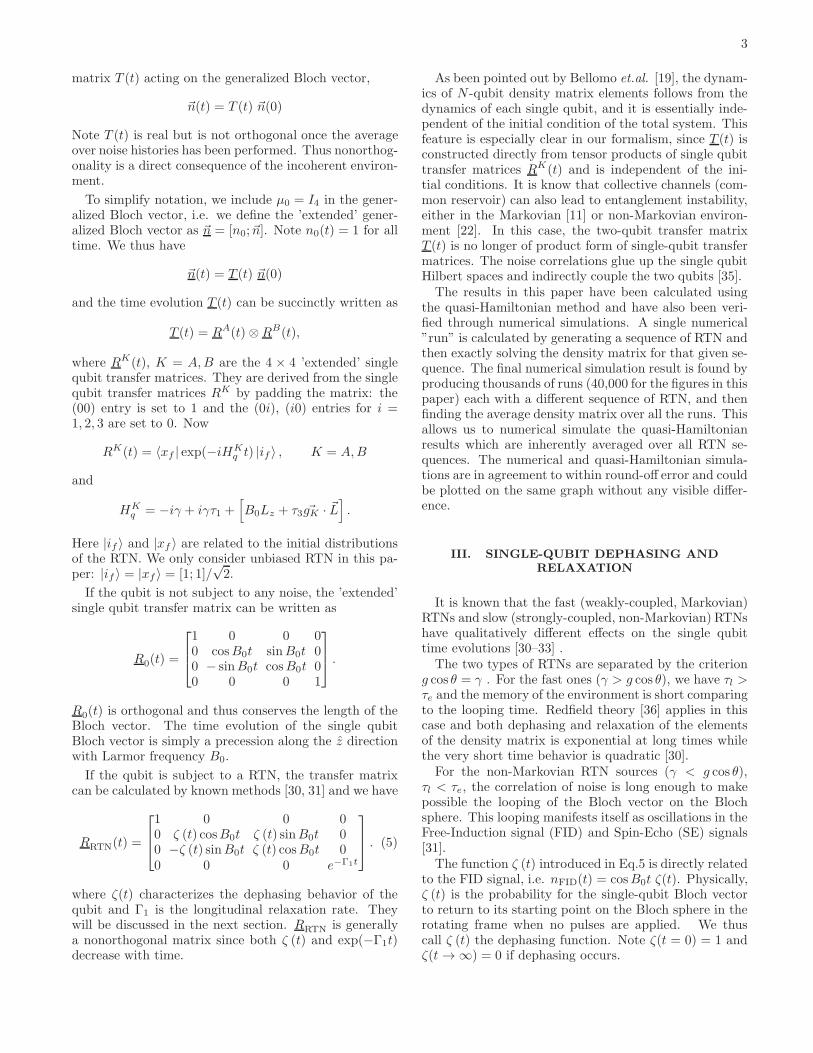
Figure 1: Pure dephasing noise for the two-one model. Toppanels (a) and (c): Square roots of eigenvalues of ρρ(t). Bot-tom panels (b) and (d): magnitude of Bloch vector n(t) aboveand concurrence CAB(t) below. These are calculated fromEqs. 20-37 and confirmed by numerical simulations. Bothqubits are operated at the pure dephasing point and onlyone of them is connected to the RTN, i.e. g1 = 0.1, g2 = 0,θ = 0. The initial state is set to

∣

∣Φ+⟩

. In (a) and (b),γ = 0.005 and the RTN is in the strong-coupling region whilein (c) and (d), γ = 0.5 and the RTN is in the weak-couplingregion. λ1 is plotted as a solid blue line, λ2 as a dashed greenline; λ3 = λ4 = 0. n(t) is plotted as a solid red line andCAB(t) as a solid black line. Time is in the unit 1/B0. Theseresults are exact.

which gives the concurrence as

CAB = 2α√

1− α2 max

{

0, |ζ(t)| − 1− e−Γ1t

2

}

= 2α√

1− α2 max {0, |ζ(t)| − ξ (t)} . (37)

The concurrence has a remarkable form. ξ (t) ≥ 0 isonly related to the longitudinal relaxation rate Γ1 andvaries between 0 for the unrelaxed state and 1/2 for thefully relaxed state; it describes relaxation only, while ζ (t)is related only to dephasing. Entanglement exists onlywhen |ζ| > ξ. The effects of dephasing (the decrease of|ζ|) and relaxation (the increase of ξ) are additive, andthey race to disentangle the state. However, ζ (t) can beoscillatory, and then revival of entanglement is possible.Once the envelope of ζ (t) is less than ξ (t), entanglementis gone for good.As a function of working point θ, Γ1 is finite except for

θ = 0: the pure dephasing point. At this point Γ1 = 0 andξ (t) = 0. Two of the four eigenvalues vanish: λ3,4 = 0.If ζ (t) is a monotonic function (weak coupling), then

CAB = 2α√1− α2|ζ(θ = 0)| > 0 at all finite times and

ESD does not occur. This is seen in Fig. 1 (c,d). Ifζ (t) is oscillatory (strong coupling) then ESD and re-vival occurs, as seen in Fig. 1 (a,b). In fact the revivalhappens an infinite number of times, since the envelopeis exponential. We again note that the result at the pure

6

dephasing point is exact; see Eqs. 12 and 13.

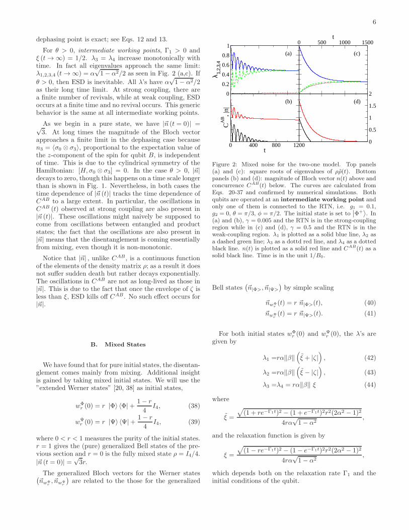
For θ > 0, intermediate working points, Γ1 > 0 andξ (t → ∞) = 1/2. λ3 = λ4 increase monotonically withtime. In fact all eigenvalues approach the same limit:λ1,2,3,4 (t → ∞) = α

√1− α2/2 as seen in Fig. 2 (a,c). If

θ > 0, then ESD is inevitable. All λ’s have α√1− α2/2

as their long time limit. At strong coupling, there area finite number of revivals, while at weak coupling, ESDoccurs at a finite time and no revival occurs. This genericbehavior is the same at all intermediate working points.

As we begin in a pure state, we have |~n (t = 0)| =√3. At long times the magnitude of the Bloch vector

approaches a finite limit in the dephasing case becausen3 = 〈σ0 ⊗ σ3〉, proportional to the expectation value ofthe z-component of the spin for qubit B, is independentof time. This is due to the cylindrical symmetry of theHamiltonian: [H,σ0 ⊗ σ3] = 0. In the case θ > 0, |~n|decays to zero, though this happens on a time scale longerthan is shown in Fig. 1. Nevertheless, in both cases thetime dependence of |~n (t)| tracks the time dependence ofCAB to a large extent. In particular, the oscillations inCAB (t) observed at strong coupling are also present in|~n (t)|. These oscillations might naively be supposed tocome from oscillations between entangled and productstates; the fact that the oscillations are also present in|~n| means that the disentanglement is coming essentiallyfrom mixing, even though it is non-monotonic.

Notice that |~n| , unlike CAB, is a continuous functionof the elements of the density matrix ρ; as a result it doesnot suffer sudden death but rather decays exponentially.The oscillations in CAB are not as long-lived as those in|~n|. This is due to the fact that once the envelope of ζ isless than ξ, ESD kills off CAB. No such effect occurs for|~n|.

B. Mixed States

We have found that for pure initial states, the disentan-glement comes mainly from mixing. Additional insightis gained by taking mixed initial states. We will use the”extended Werner states” [20, 38] as initial states,

wΦr (0) = r |Φ〉 〈Φ|+ 1− r

4I4, (38)

wΨr (0) = r |Ψ〉 〈Ψ|+ 1− r

4I4, (39)

where 0 < r < 1 measures the purity of the initial states.r = 1 gives the (pure) generalized Bell states of the pre-vious section and r = 0 is the fully mixed state ρ = I4/4.

|~n (t = 0)| =√3r.

The generalized Bloch vectors for the Werner states(

~nwΦr, ~nwΨ

r

)

are related to the those for the generalized

0

0.2

0.4

0.6

0.8

1

λ 1,2,

3,4

0 500 1000 1500t

0 400 800 1200t

CA

B, |

n|

0

0.5

1

1.5

2

(a) (c)

(b) (d)

Figure 2: Mixed noise for the two-one model. Top panels(a) and (c): square roots of eigenvalues of ρρ(t). Bottompanels (b) and (d): magnitude of Bloch vector n(t) above andconcurrence CAB(t) below. The curves are calculated fromEqs. 20-37 and confirmed by numerical simulations. Bothqubits are operated at an intermediate working point andonly one of them is connected to the RTN, i.e. g1 = 0.1,g2 = 0, θ = π/3, φ = π/2. The initial state is set to

∣

∣Φ+⟩

. In(a) and (b), γ = 0.005 and the RTN is in the strong-couplingregion while in (c) and (d), γ = 0.5 and the RTN is in theweak-coupling region. λ1 is plotted as a solid blue line, λ2 asa dashed green line; λ3 as a dottd red line, and λ4 as a dottedblack line. n(t) is plotted as a solid red line and CAB(t) as asolid black line. Time is in the unit 1/B0.

Bell states(

~n|Φ>, ~n|Ψ>

)

by simple scaling

~nwΦr(t) = r ~n|Φ>(t), (40)

~nwΨr(t) = r ~n|Ψ>(t). (41)

For both initial states wΦr (0) and wΨ

r (0), the λ’s aregiven by

λ1 =rα‖β‖(

ξ + |ζ|)

, (42)

λ2 =rα‖β‖(

ξ − |ζ|)

, (43)

λ3 =λ4 = rα‖β‖ ξ (44)

where

ξ =

√

(1 + re−Γ1t)2 − (1 + e−Γ1t)2r2(2α2 − 1)2

4rα√1− α2

,

and the relaxation function is given by

ξ =

√

(1− re−Γ1t)2 − (1− e−Γ1t)2r2(2α2 − 1)2

4rα√1− α2

,

which depends both on the relaxation rate Γ1 and theinitial conditions of the qubit.

7

00.10.20.30.40.50.6

λ 1,2,

3,4

0 200 400 600 800t

0 200 400 600 800t

CA

B, |

n|

0

0.2

0.4

0.6

0.8

(a) (c)

(b) (d)

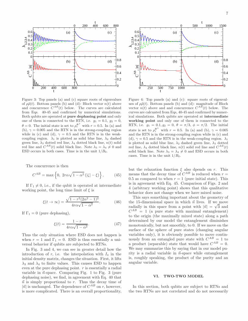
Figure 3: Top panels (a) and (c) square roots of eigenvaluesof ρρ(t). Bottom panels (b) and (d): Bloch vector n(t) aboveand concurrence CAB(t) below. The curves are calculatedfrom Eqs. 40-45 and confirmed by numerical simulations.Both qubits are operated at pure dephasing point and onlyone of them is connected to the RTN, i.e. g1 = 0.1, g2 = 0,

θ = 0. The initial state is set to ρΦ+

r with r = 0.5. In (a) and(b), γ = 0.005 and the RTN is in the strong-coupling regionwhile in (c) and (d), γ = 0.5 and the RTN is in the weak-coupling region. λ1 is plotted as solid blue line, λ2 dashedgreen line, λ3 dotted red line, λ4 dotted black line, n(t) solidred line and CAB(t) solid black line. Note λ3 = λ4 6= 0 andESD occurs in both cases. Time is in the unit 1/B0.

The concurrence is then

CAB = max{

0, 2rα√

1− α2 (|ζ| − ξ)}

, (45)

If Γ1 6= 0, i.e., if the qubit is operated at intermediateworking point, the long time limit of ξ is

ξ(t → ∞) =

√

1− r2(2α2 − 1)2

4rα√1− α2

. (46)

If Γ1 = 0 (pure dephasing),

ξ(t) =1− r

4rα√1− α2

. (47)

Thus the only situation where ESD does not happen iswhen r = 1 and Γ1 = 0. ESD is thus essentially a uni-versal behavior if qubits are subjected to RTNs.

In Fig. 3 and 4, we can see in greater detail how theintroduction of r, i.e. the interpolation with I4 in theinitial density matrix, changes the situation. First, it liftsλ3 and λ4 to finite values. This causes ESD to happeneven at the pure dephasing point. r is essentially a radialvariable in ~n-space. Comparing Fig. 1 to Fig. 3 (puredephasing noise), we find, in agreement with Eq. 40 that~n is simply proportional to r. Thus the decay time of|~n| is unchanged. The dependence of CAB on r, however,is more complicated. There is an overall proportionality,

00.10.20.30.40.50.6

λ 1,2,

3,4

0 500 1000 1500t

0 250 500 750 1000t

CA

B, |

n|

0

0.2

0.4

0.6

0.8

(a) (c)

(b) (d)

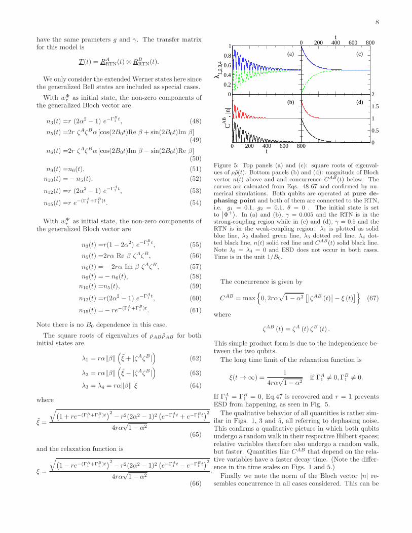
Figure 4: Top panels (a) and (c): square roots of eigenval-ues of ρρ(t). Bottom panels (b) and (d): magnitude of Blochvector n(t) above and and concurrence CAB(t) below. Thecurves are calcuated from Eqs, 40-45 and confirmed by numer-ical simulations. Both qubits are operated at intermediate

working point and only one of them is connected to theRTN, i.e. g1 = 0.1, g2 = 0, θ = π/3, φ = π/2. The initial

state is set to ρΦ+

r with r = 0.5. In (a) and (b), γ = 0.005and the RTN is in the strong-coupling region while in (c) and(d), γ = 0.5 and the RTN is in the weak-coupling region. λ1

is plotted as solid blue line, λ2 dashed green line, λ3 dottedred line, λ4 dotted black line, n(t) solid red line and CAB(t)solid black line. Note λ3 = λ4 6= 0 and ESD occurs in bothcases. Time is in the unit 1/B0.

but the relaxation function ξ also dpends on r. Thismeans that the decay time of CAB is reduced when r =0.5 as compared to when r = 1 (pure initial state). Thisis in agreement with Eq. 45. Comparison of Figs. 2 and4 (arbitrary working point) shows that this qualitativebehavior does not change when we have mixed noise.This says something important about the geometry of

the 15-dimensional space in which ~n lives. If we moveradially in this space from a point with |~n| =

√3 and

CAB = 1 (a pure state with maximal entanglement)to the origin (the maximally mixed state) along a pathdetermined by our model the entanglement diminishesmonotonically, but not smoothly, to 0. If we move on thesurface of the sphere of pure states (changing angularvariables only), it is obviously possible to move contin-uously from an entangled pure state with CAB = 1 toa product (separable) state that would have CAB = 0.We may summarize this by saying that in our model pu-rity is a radial variable in ~n-space while entanglementis, roughly speaking, the product of the purity and anangular variable.

VI. TWO-TWO MODEL

In this section, both qubits are subject to RTNs andthe two RTNs are not correlated and do not necessarily

8

have the same prameters g and γ. The transfer matrixfor this model is

T (t) = RARTN(t)⊗RB

RTN(t).

We only consider the extendedWerner states here sincethe generalized Bell states are included as special cases.

With wΦr as initial state, the non-zero components of

the generalized Bloch vector are

n3(t) =r (2α2 − 1) e−ΓB

1 t, (48)

n5(t) =2r ζAζBα [cos(2B0t)Re β + sin(2B0t)Im β](49)

n6(t) =2r ζAζBα [cos(2B0t)Im β − sin(2B0t)Re β](50)

n9(t) =n6(t), (51)

n10(t) =− n5(t), (52)

n12(t) =r (2α2 − 1) e−ΓA

1 t, (53)

n15(t) =r e−(ΓA

1 +ΓB

1 )t. (54)

With wΨr as initial state, the non-zero components of

the generalized Bloch vector are

n3(t) =r(1 − 2α2) e−ΓB

1 t, (55)

n5(t) =2rα Re β ζAζB, (56)

n6(t) =− 2rα Im β ζAζB , (57)

n9(t) =− n6(t), (58)

n10(t) =n5(t), (59)

n12(t) =r(2α2 − 1) e−ΓA

1 t, (60)

n15(t) =− re−(ΓA

1 +ΓB

1 )t. (61)

Note there is no B0 dependence in this case.

The square roots of eigenvalues of ρAB ρAB for bothinitial states are

λ1 = rα‖β‖(

ξ + |ζAζB |)

(62)

λ2 = rα‖β‖(

ξ − |ζAζB |)

(63)

λ3 = λ4 = rα‖β‖ ξ (64)

where

ξ =

√

(

1 + re−(ΓA

1+ΓB

1)t)2 − r2(2α2 − 1)2

(

e−ΓA

1t + e−ΓB

1t)2

4rα√1− α2

(65)

and the relaxation function is

ξ =

√

(

1− re−(ΓA

1+ΓB

1)t)2 − r2(2α2 − 1)2

(

e−ΓA

1t − e−ΓB

1t)2

4rα√1− α2

.

(66)

0

0.2

0.4

0.6

0.8

1

λ 1,2,

3,4

0 200 400 600 800t

0 200 400 600 800t

CA

B, |

n|

0

0.5

1

1.5

2

(a) (c)

(b) (d)

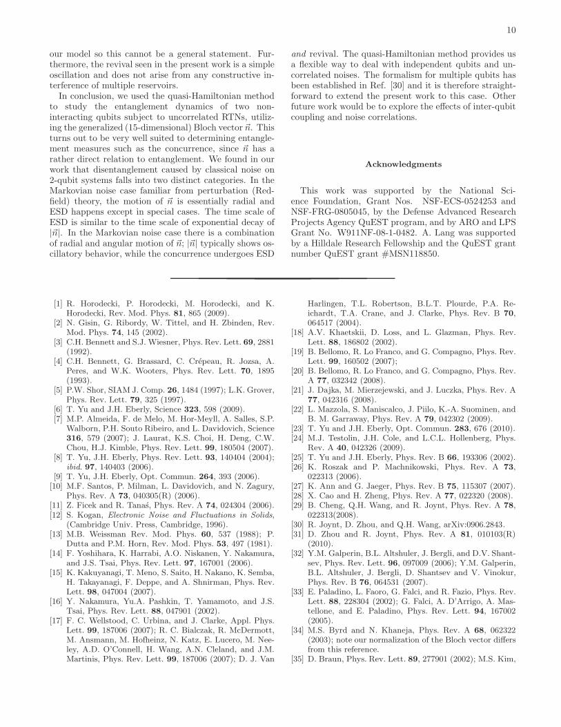
Figure 5: Top panels (a) and (c): square roots of eigenval-ues of ρρ(t). Bottom panels (b) and (d): magnitude of Blochvector n(t) above and and concurrence CAB(t) below. Thecurves are calcuated from Eqs. 48-67 and confirmed by nu-merical simulations. Both qubits are operated at pure de-

phasing point and both of them are connected to the RTN,i.e. g1 = 0.1, g2 = 0.1, θ = 0 . The initial state is setto

∣

∣Φ+⟩

. In (a) and (b), γ = 0.005 and the RTN is in thestrong-coupling region while in (c) and (d), γ = 0.5 and theRTN is in the weak-coupling region. λ1 is plotted as solidblue line, λ2 dashed green line, λ3 dotted red line, λ4 dot-ted black line, n(t) solid red line and CAB(t) solid black line.Note λ3 = λ4 = 0 and ESD does not occur in both cases.Time is in the unit 1/B0.

The concurrence is given by

CAB = max{

0, 2rα√

1− α2[∣

∣ζAB (t)∣

∣− ξ (t)]

}

(67)

where

ζAB (t) = ζA (t) ζB (t) .

This simple product form is due to the independence be-tween the two qubits.

The long time limit of the relaxation function is

ξ(t → ∞) =1

4rα√1− α2

if ΓA1 6= 0,ΓB

1 6= 0.

If ΓA1 = ΓB

1 = 0, Eq.47 is recovered and r = 1 preventsESD from happening, as seen in Fig. 5.

The qualitative behavior of all quantities is rather sim-ilar in Figs. 1, 3 and 5, all referring to dephasing noise.This confirms a qualitative picture in which both qubitsundergo a random walk in their respective Hilbert spaces;relative variables therefore also undergo a random walk,but faster. Quantities like CAB that depend on the rela-tive variables have a faster decay time. (Note the differ-ence in the time scales on Figs. 1 and 5.)

Finally we note the norm of the Bloch vector |n| re-sembles concurrence in all cases considered. This can be

9

0 π/2θ

0

1

g/γ

OSC

EXP

Figure 6: ”Phase diagram” of the behavior of CAB(t), given’extended’ Werner state as initial state. In the upper region,we have ESD and revival before CAB goes permanently tozero. In the lower region, CAB dies just once and for all.

seen from the explicit expression

|n| = r

√

√

√

√

8α2(1− α2)(

ζAB)2

+ e−2(ΓA

1 t+ΓB

1 t)

+(1− 2α2)2[

e−2ΓA

1 t + e−2ΓB

1 t] . (68)

Since the generalized Bloch vector fully describes the sys-tem, a geometric picture of ~n for entanglement might bepossible. To our knowledge, such a description is notyet available except for some special parameterized states[39] or close to ~n = ~0 [40].

VII. DISCUSSION AND CONCLUSION

The most important conclusion of the paper is thatthe disentangling effect of non-Markovian, or strongly-coupled, noise and the effect of Markovian, or weakly-coupled, noise is qualitatively different. In Sec. V andVI, we see CAB(t) can take on two forms before ESDoccurs: oscillatory and exponential, depending on thecoupling of the RTN. By numerical exploration, we haveconstructed the ”phase diagram” in Fig. 6, where theboundary is given by

g/γ = sec θ.

The oscillatory behavior arises from looping of ~n onthe Bloch sphere. This can only occur if the noise is slowenough that the topology if the sphere is fully exploredbefore the Bloch vector decays entirely. If the noise isfast, the relaxation moves ~n along a radial path to theorigin no looping occurs.

If the noise acts only on one qubit, the two-one model,the situation can be analyzed in some detail. Qubit Bis not subject to RTN and is stationary in the rotatingframe. It effectively serves as a reference and the two-qubit concurrence is fully determined by qubit A, as seenin Eq. 37.

Figure 7: Single-qubit Bloch representation of the two-onemodel. Initial states are the generalized Bell states. Insidethe cone CAB = 0.

In the single-qubit Bloch sphere picture,

|ζ| = ρA| sin θA| (69)

e−Γ1t = ρA cos θA, (70)

where ρA and θA are the length and polar angle of thethree dimensional Bloch vector of qubit A.Given generalized Bell states as initial state, CAB = 0

is equivalent to

2ρA| sin θA|+ ρA cos θA ≤ 1.

Geometrically, it means CAB = 0 as long as qubit A’sBloch vector falls inside the cone shown in Fig. 7.In the two-two model, however, both qubits have non-

trivial time evolution. This simple one-qubit picture forconcurrence then does not work and one needs to treatthe full 15-dimensional Bloch vector for the whole sys-tem.One important question is the relation of this work to

previous results on single qubits [31–33]. The oscillationsthat occur in |~n| and CAB are clearly related to the noise-induced looping on the single-qubit Bloch sphere. Forexample, they have the same period. However, in thesingle-qubit case these oscillations occur in the tails of anoverall Gaussian decay. They are much more pronouncedin |~n| and CAB.Entanglement revival was introduced in Ref. [11] and

later on shown to exist in different systems [19, 41]. It hassometimes been attributed to back-action from the non-Markovian environment [22]. There is no back-action in

10

our model so this cannot be a general statement. Fur-thermore, the revival seen in the present work is a simpleoscillation and does not arise from any constructive in-terference of multiple reservoirs.In conclusion, we used the quasi-Hamiltonian method

to study the entanglement dynamics of two non-interacting qubits subject to uncorrelated RTNs, utiliz-ing the generalized (15-dimensional) Bloch vector ~n. Thisturns out to be very well suited to determining entangle-ment measures such as the concurrence, since ~n has arather direct relation to entanglement. We found in ourwork that disentanglement caused by classical noise on2-qubit systems falls into two distinct categories. In theMarkovian noise case familiar from perturbation (Red-field) theory, the motion of ~n is essentially radial andESD happens except in special cases. The time scale ofESD is similar to the time scale of exponential decay of|~n|. In the Markovian noise case there is a combinationof radial and angular motion of ~n; |~n| typically shows os-cillatory behavior, while the concurrence undergoes ESD

and revival. The quasi-Hamiltonian method provides usa flexible way to deal with independent qubits and un-correlated noises. The formalism for multiple qubits hasbeen established in Ref. [30] and it is therefore straight-forward to extend the present work to this case. Otherfuture work would be to explore the effects of inter-qubitcoupling and noise correlations.

Acknowledgments

This work was supported by the National Sci-ence Foundation, Grant Nos. NSF-ECS-0524253 andNSF-FRG-0805045, by the Defense Advanced ResearchProjects Agency QuEST program, and by ARO and LPSGrant No. W911NF-08-1-0482. A. Lang was supportedby a Hilldale Research Fellowship and the QuEST grantnumber QuEST grant #MSN118850.

[1] R. Horodecki, P. Horodecki, M. Horodecki, and K.Horodecki, Rev. Mod. Phys. 81, 865 (2009).

[2] N. Gisin, G. Ribordy, W. Tittel, and H. Zbinden, Rev.Mod. Phys. 74, 145 (2002).

[3] C.H. Bennett and S.J. Wiesner, Phys. Rev. Lett. 69, 2881(1992).

[4] C.H. Bennett, G. Brassard, C. Crepeau, R. Jozsa, A.Peres, and W.K. Wooters, Phys. Rev. Lett. 70, 1895(1993).

[5] P.W. Shor, SIAM J. Comp. 26, 1484 (1997); L.K. Grover,Phys. Rev. Lett. 79, 325 (1997).

[6] T. Yu and J.H. Eberly, Science 323, 598 (2009).[7] M.P. Almeida, F. de Melo, M. Hor-Meyll, A. Salles, S.P.

Walborn, P.H. Souto Ribeiro, and L. Davidovich, Science316, 579 (2007); J. Laurat, K.S. Choi, H. Deng, C.W.Chou, H.J. Kimble, Phys. Rev. Lett. 99, 180504 (2007).

[8] T. Yu, J.H. Eberly, Phys. Rev. Lett. 93, 140404 (2004);ibid. 97, 140403 (2006).

[9] T. Yu, J.H. Eberly, Opt. Commun. 264, 393 (2006).[10] M.F. Santos, P. Milman, L. Davidovich, and N. Zagury,

Phys. Rev. A 73, 040305(R) (2006).[11] Z. Ficek and R. Tanas, Phys. Rev. A 74, 024304 (2006).[12] S. Kogan, Electronic Noise and Fluctuations in Solids,

(Cambridge Univ. Press, Cambridge, 1996).[13] M.B. Weissman Rev. Mod. Phys. 60, 537 (1988); P.

Dutta and P.M. Horn, Rev. Mod. Phys. 53, 497 (1981).[14] F. Yoshihara, K. Harrabi, A.O. Niskanen, Y. Nakamura,

and J.S. Tsai, Phys. Rev. Lett. 97, 167001 (2006).[15] K. Kakuyanagi, T. Meno, S. Saito, H. Nakano, K. Semba,

H. Takayanagi, F. Deppe, and A. Shnirman, Phys. Rev.Lett. 98, 047004 (2007).

[16] Y. Nakamura, Yu.A. Pashkin, T. Yamamoto, and J.S.Tsai, Phys. Rev. Lett. 88, 047901 (2002).

[17] F. C. Wellstood, C. Urbina, and J. Clarke, Appl. Phys.Lett. 99, 187006 (2007); R. C. Bialczak, R. McDermott,M. Ansmann, M. Hofheinz, N. Katz, E. Lucero, M. Nee-ley, A.D. O’Connell, H. Wang, A.N. Cleland, and J.M.Martinis, Phys. Rev. Lett. 99, 187006 (2007); D. J. Van

Harlingen, T.L. Robertson, B.L.T. Plourde, P.A. Re-ichardt, T.A. Crane, and J. Clarke, Phys. Rev. B 70,064517 (2004).

[18] A.V. Khaetskii, D. Loss, and L. Glazman, Phys. Rev.Lett. 88, 186802 (2002).

[19] B. Bellomo, R. Lo Franco, and G. Compagno, Phys. Rev.Lett. 99, 160502 (2007);

[20] B. Bellomo, R. Lo Franco, and G. Compagno, Phys. Rev.A 77, 032342 (2008).

[21] J. Dajka, M. Mierzejewski, and J. Luczka, Phys. Rev. A77, 042316 (2008).

[22] L. Mazzola, S. Maniscalco, J. Piilo, K.-A. Suominen, andB. M. Garraway, Phys. Rev. A 79, 042302 (2009).

[23] T. Yu and J.H. Eberly, Opt. Commun. 283, 676 (2010).[24] M.J. Testolin, J.H. Cole, and L.C.L. Hollenberg, Phys.

Rev. A 40, 042326 (2009).[25] T. Yu and J.H. Eberly, Phys. Rev. B 66, 193306 (2002).[26] K. Roszak and P. Machnikowski, Phys. Rev. A 73,

022313 (2006).[27] K. Ann and G. Jaeger, Phys. Rev. B 75, 115307 (2007).[28] X. Cao and H. Zheng, Phys. Rev. A 77, 022320 (2008).[29] B. Cheng, Q.H. Wang, and R. Joynt, Phys. Rev. A 78,

022313(2008).[30] R. Joynt, D. Zhou, and Q.H. Wang, arXiv:0906.2843.[31] D. Zhou and R. Joynt, Phys. Rev. A 81, 010103(R)

(2010).[32] Y.M. Galperin, B.L. Altshuler, J. Bergli, and D.V. Shant-

sev, Phys. Rev. Lett. 96, 097009 (2006); Y.M. Galperin,B.L. Altshuler, J. Bergli, D. Shantsev and V. Vinokur,Phys. Rev. B 76, 064531 (2007).

[33] E. Paladino, L. Faoro, G. Falci, and R. Fazio, Phys. Rev.Lett. 88, 228304 (2002); G. Falci, A. D’Arrigo, A. Mas-tellone, and E. Paladino, Phys. Rev. Lett. 94, 167002(2005).

[34] M.S. Byrd and N. Khaneja, Phys. Rev. A 68, 062322(2003); note our normalization of the Bloch vector differsfrom this reference.

[35] D. Braun, Phys. Rev. Lett. 89, 277901 (2002); M.S. Kim,

11

J. Lee, D. Ahn, and P.L. Knight, Phys. Rev. A 65,040101(R) (2002); J.P. Paz and A.J. Roncaglia, Phys.Rev. Lett. 100, 220401 (2008).

[36] C. P. Slichter, Principles of Magnetic Resonance, 3rd ed.(Springer, New York, 1996).

[37] W.K. Wootters, Phys. Rev. Lett. 80, 2245 (1998).[38] R.F. Werner, Phys. Rev. A 40, 4277 (1989).[39] R.A. Bertlmann and P. Krammer, arXiv:0706.1743

(2007).

[40] S.L. Braunstein, C.M. Caves, R. Jozsa, N. Linden, S.Popescu, and R. Schack, Phys. Rev. Lett. 83, 1054(1999); W. Dur, J.I. Cirac, and R. Tarrach, i.b.i.d 83,3562 (1999); L. Gurvits and H. Barnum, Phys. Rev. A68, 042312 (2003); L. Gurvits and H. Barnum, i.b.i.d 72,032322 (2005).

[41] S. Maniscalco, F. Francica, R.L. Zaffino, N. Lo Gullo,and F. Plastina, Phys. Rev. Lett. 100, 090503 (2008).