electronic reprint IUCrJ ISSN: 2052-2525 www.iucrj.org Quantitative disentanglement of nanocrystalline phases in cement pastes by synchrotron ptychographic X-ray tomography Ana Cuesta, ´ Angeles G. De la Torre, Isabel Santacruz, Ana Diaz, Pavel Trtik, Mirko Holler, Barbara Lothenbach and Miguel A. G. Aranda IUCrJ (2019). 6, 473–491 IUCr Journals CRYSTALLOGRAPHY JOURNALS ONLINE This open-access article is distributed under the terms of the Creative Commons Attribution Licence http://creativecommons.org/licenses/by/4.0/legalcode, which permits unrestricted use, distribution, and reproduction in any medium, provided the original authors and source are cited. IUCrJ (2019). 6, 473–491 Cuesta et al. · Disentanglement of nanocrystalline phases by X-ray tomography

Welcome message from author
This document is posted to help you gain knowledge. Please leave a comment to let me know what you think about it! Share it to your friends and learn new things together.
Transcript
electronic reprint
IUCrJISSN: 2052-2525
www.iucrj.org
Quantitative disentanglement of nanocrystalline phases incement pastes by synchrotron ptychographic X-raytomography
Ana Cuesta, Angeles G. De la Torre, Isabel Santacruz, Ana Diaz, PavelTrtik, Mirko Holler, Barbara Lothenbach and Miguel A. G. Aranda
IUCrJ (2019). 6, 473–491
IUCr JournalsCRYSTALLOGRAPHY JOURNALS ONLINE
This open-access article is distributed under the terms of the Creative Commons Attribution Licencehttp://creativecommons.org/licenses/by/4.0/legalcode, which permits unrestricted use, distribution, andreproduction in any medium, provided the original authors and source are cited.
IUCrJ (2019). 6, 473–491 Cuesta et al. · Disentanglement of nanocrystalline phases by X-ray tomography
research papers
IUCrJ (2019). 6, 473–491 https://doi.org/10.1107/S2052252519003774 473
IUCrJISSN 2052-2525
NEUTRONjSYNCHROTRON
Received 14 November 2018
Accepted 19 March 2019
Edited by I. Robinson, UCL, UK
Keywords: Portland cement; X-ray imaging;
microstructure determination; density measure-
ments; C-S-H gels; amorphous hydrogarnet;
synchrotron ptychographic tomography;
nanocrystalline components; thermodynamic
modelling.
Supporting information: this article has
supporting information at www.iucrj.org
Quantitative disentanglement of nanocrystallinephases in cement pastes by synchrotronptychographic X-ray tomography
Ana Cuesta,a Angeles G. De la Torre,a Isabel Santacruz,a Ana Diaz,b Pavel Trtik,b,c
Mirko Holler,b Barbara Lothenbachd and Miguel A. G. Arandae,a*
aDepartamento de Quımica Inorganica, Cristalografıa y Mineralogıa, Universidad de Malaga, 29071-Malaga, Spain, bPaul
Scherrer Institut, 5232 Villigen PSI, Switzerland, cFaculty of Civil Engineering, Czech Technical University in Prague,
166 29 Prague, Czech Republic, dEMPA, Laboratory for Concrete and Construction Chemistry, Uberlandstrasse 129,
CH-8600 Dubendorf, Switzerland, and eALBA Synchrotron, Carrer de la Llum 2-26, E-08290 Cerdanyola del Valles,
Barcelona, Spain. *Correspondence e-mail: [email protected], [email protected]
Mortars and concretes are ubiquitous materials with very complex hierarchical
microstructures. To fully understand their main properties and to decrease their
CO2 footprint, a sound description of their spatially resolved mineralogy is
necessary. Developing this knowledge is very challenging as about half of the
volume of hydrated cement is a nanocrystalline component, calcium silicate
hydrate (C-S-H) gel. Furthermore, other poorly crystalline phases (e.g. iron
siliceous hydrogarnet or silica oxide) may coexist, which are even more difficult
to characterize. Traditional spatially resolved techniques such as electron
microscopy involve complex sample preparation steps that often lead to
artefacts (e.g. dehydration and microstructural changes). Here, synchrotron
ptychographic tomography has been used to obtain spatially resolved
information on three unaltered representative samples: neat Portland paste,
Portland–calcite and Portland–fly-ash blend pastes with a spatial resolution
below 100 nm in samples with a volume of up to 5 � 104 mm3. For the neat
Portland paste, the ptychotomographic study gave densities of 2.11 and
2.52 g cm�3 and a content of 41.1 and 6.4 vol% for nanocrystalline C-S-H gel
and poorly crystalline iron siliceous hydrogarnet, respectively. Furthermore, the
spatially resolved volumetric mass-density information has allowed character-
ization of inner-product and outer-product C-S-H gels. The average density of
the inner-product C-S-H is smaller than that of the outer product and its
variability is larger. Full characterization of the pastes, including segmentation
of the different components, is reported and the contents are compared with the
results obtained by thermodynamic modelling.
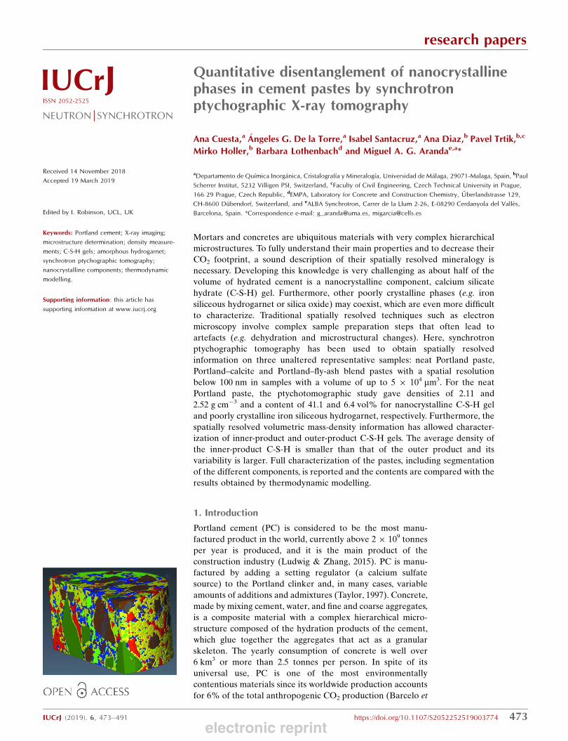
1. Introduction
Portland cement (PC) is considered to be the most manu-
factured product in the world, currently above 2 � 109 tonnes
per year is produced, and it is the main product of the
construction industry (Ludwig & Zhang, 2015). PC is manu-
factured by adding a setting regulator (a calcium sulfate
source) to the Portland clinker and, in many cases, variable
amounts of additions and admixtures (Taylor, 1997). Concrete,
made by mixing cement, water, and fine and coarse aggregates,
is a composite material with a complex hierarchical micro-
structure composed of the hydration products of the cement,
which glue together the aggregates that act as a granular
skeleton. The yearly consumption of concrete is well over
6 km3 or more than 2.5 tonnes per person. In spite of its
universal use, PC is one of the most environmentally
contentious materials since its worldwide production accounts
for 6% of the total anthropogenic CO2 production (Barcelo et
electronic reprint
al., 2014). Hence, there are many ongoing research efforts to
better understand cement hydration chemistry in order to
reduce its CO2 footprint in a safe, economic and sustainable
way.
The hydration products of cement depend upon its
elemental and mineralogical composition, texture and the
hydration conditions: water-to-cement ratio, temperature,
pressure, presence of admixtures etc. We shall not go into
detail about this here but the interested reader is recom-
mended to read the classical books on the chemistry of
cements (Bensted & Barnes, 2002; Taylor, 1997) and recent
books for state-of-the-art characterization techniques (Scri-
vener et al., 2016; Pollmann, 2017). The main component
phases of the hydration of PC are nanocrystalline calcium
silicate hydrate (C-S-H) gels, crystalline portlandite, Ca(OH)2
and crystalline ettringite, Ca6Al2(SO4)3(OH)12�26H2O. More-
over, Fe–Al siliceous hydrogarnet, the main iron-containing
phase, has been reported to form in PC, based on X-ray
powder diffraction and X-ray absorption spectroscopy studies
(Dilnesa, Wieland et al., 2014; Vespa et al., 2015). Its obser-
vation and quantification is, in the presence of nanocrystalline
C-S-H, difficult and challenging because of its poorly ordered
nature.
Furthermore, plain PC can be mixed with additional
compounds to decrease the production cost, to lower the CO2
footprint and to improve performance. The main addition to
plain PC in concrete production is calcite and supplementary
cementitious materials (SCM) (Pacewska & Wilinska, 2013;
Scrivener et al., 2015; Juenger & Siddique, 2015). SCMs
include fly ash (FA), ground granulated blast-furnace slag,
calcined clays, natural pozzolans and silica fume.
It is widely accepted that the strength and other mechanical
and chemical properties of mortars and concretes mainly rely
upon the formation of C-S-H gel during cement hydration
which forms about half the volume of all cement hydrates
(Taylor, 1997; Bensted & Barnes, 2002). Because of the
complex hierarchical arrangement of cement pastes in general
(Mehta et al., 2014), and C-S-H gel in particular (Papatzani et
al., 2015; Cuesta et al., 2018; Andalibi et al., 2018; Kumar et al.,
2017), techniques yielding spatially resolved information are
key to their characterization. There are different approaches
for obtaining spatially resolved information including scan-
ning electron microscopy, transmission electron microscopy,
nanoindentation and X-ray imaging. Here, we will focus only
on synchrotron X-ray imaging techniques (Aranda, 2016)
which allow the investigation of samples or pastes without the
need for a preparation step before measurements are made,
thus avoiding many artefacts caused by such preparations.
Since the pioneering work of Bentz et al. (2000), absorption-
contrast X-ray computed tomography has been widely used
for investigating PC hydration and to study several parameters
under different conditions, including the pore and void
network (Gallucci et al., 2007; Moradian et al., 2017), tortu-
osity (Promentilla et al., 2009, 2016), leaching alterations
(Sugiyama et al., 2010), alkali–silica reactions (Marinoni et al.,
2012; Voltolini et al., 2011; Hernandez-Cruz et al., 2016), early
hydration microstructure evolution (Gastaldi et al., 2012;
Parisatto et al., 2015) and uranium encapsulation in grout (Stitt
et al., 2017, 2018). As of today, these tomographic investiga-
tions have limited spatial resolution (usually 500 nm at best)
and it is extremely difficult to distinguish between different
hydrated phases as they have very similar X-ray absorption
values (Deboodt et al., 2017) yielding poor contrast. Phase-
contrast tomography has also been applied to PC pastes but
the final attained spatial resolution was close to 10 mm (Yang
et al., 2016).
One step forward in X-ray computed tomography involves
the use of the diffraction signal (Birkbak et al., 2015). This
technique combines the merits of diffraction with computed
tomography to allow imaging of the interior of materials, for
instance determining the distributions of polymorphs in
complex mixtures, by using a focused synchrotron beam and
measuring the diffraction or scattering signal arising from the
nano- or atomic structure of the specimen in a raster-scanning
approach. This technique has also been widely applied to
cements (Artioli et al., 2010; Valentini et al., 2011, 2012;
Voltolini et al., 2013), e.g. to unravel the change of nucleation
mechanism in cements when adding polycarboxylate ether
superplasticizers (Artioli et al., 2015) and to better understand
the microstructural signature of carbonation in blended
cement pastes (Claret et al., 2018). Unfortunately, the best
spatial resolution attainable today with this technique, �4 mm,
does not allow the hierarchical arrangement of the component
phases in the key 100–5000 nm mesoscale range to be
understood.
The state-of-the-art evolution of these synchrotron imaging
techniques brings us to X-ray ptychography, a scanning tech-
nique that makes use of the coherent properties of synchro-
tron radiation (Dierolf et al., 2010). In coherent diffraction
imaging, the post-sample X-ray optics are replaced by phase-
retrieval algorithms which, combined with the ptychographic
approach (scanning a sample at overlapping illumination areas
of the sample), makes this technique robust and reliable
(Rodenburg et al., 2007; Guizar-Sicairos & Fienup, 2008;
Thibault et al., 2009; Faulkner & Rodenburg, 2004). A focused
hard-X-ray synchrotron beam is used to illuminate the sample
and coherent diffraction patterns are recorded in the far field.
The diversity in the data arising from acquisitions at over-
lapping areas of the specimen and the use of iterative phase-
retrieval algorithms yield both the amplitude and the phase of
the complex-valued transmissivity of the sample. X-ray
ptychography provides 2D high-resolution projections of the
sample. Ptychographic X-ray computed tomography (PXCT)
(Dierolf et al., 2010) combines ptychography and tomography
to simultaneously provide two volumes with a 3D distribution
of the difference from the real part of the refractive index,
�(r), and the imaginary part of the refractive index, �(r). Thus,
the complete complex-valued refractive index of the sample,
n(r) = 1 � �(r) + i�(r), can be obtained (da Silva et al., 2015).
We note that this procedure gives two tomograms per
measurement with complementary information, volumetric
electron density and X-ray attenuation. PXCT can provide
isotropic 3D resolution better than 20 nm (Holler et al., 2014)
and accurate volumetric mass density values when the stoi-
research papers
474 Cuesta et al. � Disentanglement of nanocrystalline phases by X-ray tomography IUCrJ (2019). 6, 473–491
electronic reprint
chiometries are known (Diaz et al., 2012), which makes the
technique appropriate for analysing the microstructures of
cement pastes (Trtik et al., 2013; da Silva et al., 2015; Cuesta et
al., 2017a), as the densities of every component within
complex mixtures can be mapped out with a high spatial
resolution. Hereafter, the term density is used only when
referring to volumetric mass density. Volumetric electron
density is abbreviated to just electron density. PXCT has been
applied to investigate the hydration, composition, density and
microstructure of a PC paste (Trtik et al., 2013) although the
reported mass densities were affected by the resin-impregna-
tion procedure employed. The 3D maps of all the individual
phases were segmented and their mass densities were quan-
titatively determined. Moreover, the densities and water
content of the C-S-H gels were also determined (da Silva et al.,
2015) for an alite paste with a high water-to-alite ratio. We
have recently used this technique to determine the ettringite
and gel volume distributions in the segmented tomograms of
calcium sulfoaluminate pastes (Cuesta et al., 2017a). In this
work, the composition and density of two aluminium hydro-
xide amorphous gel agglomerates were determined. The in situ
hydration of a sample of ye’elimite with gypsum at different
early stages, between 48 and 63 h, was also followed by PXCT
(Cuesta et al., 2017b). Finally, we are aware of the use of
ptychography with soft X-rays for studying different types of
cement pastes (Bae et al., 2015; Geng, Li et al., 2017; Geng,
Myers et al., 2017; Geng et al., 2018). The high spatial resolu-
tion of this approach is adequate for studying the arrangement
of some components within the pastes but the small field of
view precludes the quantification of the different components.
In this work, we have used PXCT to study three cement
pastes: neat PC, PC blended with calcite and PC blended with
FA. In addition to full segmentation, and so quantitative
component analysis, several parameters have been deter-
mined, which constitutes a significant advance in the under-
standing of cement chemistry.
2. Materials and methods
2.1. Cement pastes
Commercial PC from FYM SA (Malaga, Spain), FA Class F
supplied by a power station in Lada (Spain) (Garcıa-Matere et
al., 2013) and CaCO3 (calcite, 99.0%) from Sigma–Aldrich
were used for this study. Their chemical and mineralogical
analyses are given in the Supporting information. Three pastes
were studied in this work. These were prepared by mixing the
appropriate cement with water in a two-step approach: cement
preparation and a water-mixing procedure. The cement
samples were prepared as follows.
(a) Neat PC. Commercial cement was milled for 40 min in a
vibratory ball mill. The PC was milled to ensure that large
particles could not block the narrow parts of the capillaries,
see Fig. S1(a).
(b) PC–CC blend. A mixture of 80 wt% of PC and 20 wt%
of CaCO3 was prepared by homogenizing the blend in an
agate mortar for 15 min. Previously, PC was milled as indi-
cated above. Calcite was attrition milled with isopropanol for
10 min, see Fig. S1(b).
(c) PC–FA blend. A mixture of 70 wt% of PC and 30 wt%
of FA was prepared with the same procedure described above.
The initial particle size distribution of FA is reported in Fig.
S1(c). Additionally, the blend was milled for 30 min in a
vibratory ball mill and was then attrition milled with iso-
propanol for 30 min.
The long milling times can increase the temperature and
could even lead to partial dehydration of gypsum. This
possible change in the sulfates could have an effect on the
early stage hydration kinetics but it should not significantly
modify the hydration phase assemblage at later stages, e.g.
after five months as studied here.
The three cement samples were loaded inside tapering
quartz capillaries. An ultrasound bath was used to shake the
capillaries in order to help the powder to reach the tip. The
possible separation of particles in this process cannot be ruled
out. However the effect, if it takes place, must be minor given
the agreement between the content of the determined
component phases and the results from the thermodynamic
modelling of the nominal starting composition (see below).
The capillary was then filled up with an adequate amount of
distilled water and both ends of the capillary were sealed
immediately with UV-hardening glue. The pastes within the
quartz capillaries were stored at room temperature and
investigated at the cSAXS beamline after five months of
hydration.
2.2. PXCT experiment
The three cement pastes were measured at the cSAXS
beamline at the Swiss Light Source, Paul Scherrer Institute
(Villigen, Switzerland) using the instrument already described
in a previous work (Holler et al., 2014). The photon energy of
the X-ray beam was 6.2 keV. Diffraction patterns were
collected with an EIGER 500K detector placed 7.305 m
downstream of the sample satisfying the ptychography
sampling conditions (Edo et al., 2013; da Silva & Menzel,
2015). For the PC sample, the total acquisition time for all
diffraction patterns including the time necessary for sample
positioning was 17 h. For the PC–CC and PC–FA blends, the
total acquisition times were 22 and 20 h, respectively. Addi-
tional experimental details about the measurements can be
found in the Supporting information. Some limitations apply
to PXCT that can be sample dependent, for example, radia-
tion damage, which is mostly a problem for soft condensed
matter and labile samples. Another limitation is the width of
the samples to be imaged. Very thick samples do not allow
enough X-ray penetration and may lead to a very large phase
shift that could be difficult to invert. The sample thickness can
also limit the achievable spatial resolution in the 2D projec-
tion images due to a limit on the depth of focus. This limitation
affects any microscopy method, but in the case of ptycho-
graphy it can be overcome, as discussed by Tsai et al. (2016).
Because of its high resolution and its capability to provide
quantitative absorption and phase contrast, PXCT is starting
research papers
IUCrJ (2019). 6, 473–491 Cuesta et al. � Disentanglement of nanocrystalline phases by X-ray tomography 475electronic reprint
to be used for the characterization of a wide range of mate-
rials, from integrated circuits (Holler et al., 2017) to frozen-
hydrated brain tissue (Shahmoradian et al., 2017).
2.3. PXCT data processing and analysis
The ptychography reconstructions were carried out using a
difference-map algorithm (Thibault et al., 2009) followed by a
maximum-likelihood refinement (Thibault & Guizar-Sicairos,
2012). The pixel size of the reconstructed projections was
38.95 nm. The spatial resolution of the tomograms was
determined by Fourier shell correlation (FSC) with a
threshold based on the half-bit criterion (Holler et al., 2014;
van Heel & Schatz, 2005). Further specific details about the
tomographic reconstructions (Guizar-Sicairos et al., 2011) can
be found in the Supporting information.
The 3D electron-density distribution, ne(r), can be deter-
mined as follows (Diaz et al., 2012)
ne rð Þ ¼ 2�� rð Þr0�
2; ð1Þ
where r0 is the classical electron radius and � is the X-ray
wavelength. The density can be obtained as
� rð Þ ¼ ne rð ÞANAZ
; ð2Þ
where NA is Avogadro’s number, A is the molar mass, and Z is
the total number of electrons in the formula unit.
Moreover, the linear attenuation coefficient, �, can be
calculated by using equation (3) (da Silva et al., 2015)
� rð Þ ¼ 4�
�
�� rð Þ
�: ð3Þ
The next stage was detailed spatial characterization of
selected component phases. Many component particles were
chosen and the spatial distribution of their electron densities
was thoroughly studied. The analysis was performed by
monitoring the evolution of the electron-density value along
selected directions. This characterization was carried out with
ImageJ/Fuji shareware (Abramoff et al., 2004; Schindelin et al.,
2012).
Following this, the segmentation of the component phases
was carried out. A region of interest of each sample was
selected to perform threshold-based image segmentation
initially on the phase-contrast tomogram. The segmentation
study was performed with Avizo Fire v. 8.0 (FEI Visualization
Sciences Group). All the materials were separated using the
average values obtained for the electron densities by applying
the threshold tool which is included in the segmentation editor
of the Avizo suite. The borders of the regions were smoothed.
Finally, the volume percentages of each phase were quanti-
tatively determined using the material statistics tool of the
Avizo suite. Moreover, the average electron-density values for
every component were also obtained from these segmented
volumes.
The quality [signal-to-noise (s/n) ratio] and spatial resolu-
tion of the absorption tomograms were poorer than those of
the phase-contrast tomograms. This is an inherent feature in
the transmissivity of a sample with hard X-rays, i.e. X-rays with
an energy above about 2 keV, where absorption is much
weaker compared with the phase shift. Consequently, the 3D
segmented masks of the material phases based on the phase-
contrast tomograms were used in the amplitude tomograms to
obtain the attenuation coefficient based on the � values for the
main mineralogical phases. In addition, the Shrink tool was
applied for these tomograms. This tool applies morphological
erosion of the mask using a structural element that includes
the voxel of origin and its connection to neighbouring voxels.
Moreover, and very importantly, for phases with very
similar electron densities, because of the difficulty of distin-
guishing them in the phase-contrast tomogram, the �(r)
dataset was also used to perform the segmentation procedure.
In these cases, the segmented masks were created by providing
the lower and upper bounds for both � and � values obtained
from the bivariate histogram (see below).
2.4. Thermodynamic modelling
Thermodynamic modelling was carried out using Gibbs free
energy minimization software (GEMs 3.4; Wagner et al., 2012;
Kulik et al., 2013) which calculates the equilibrium phase
assemblages in chemical systems from their total bulk
elemental composition. The default databases were expanded
with the CEMDATA18 database (Lothenbach et al., 2019); C-
S-H was modelled with the CSH-II model, and the Parrot and
Killoh model was used for the hydration modelling (Lothen-
bach et al., 2008). The CSH-II model was selected because it
has 2.1 H2O/Si for C-S-H without gel water and a high Ca/Si
ratio for the mineral phase, which results in adequate overall
water content, close to 4.0 water molecules per mol of Si which
includes gel water, and density values in agreement with the
measurements of Muller et al. (2013). Conversely, the water
content for C-S-H without gel water in the more recent CSHQ
model is 3 H2O/Si, which is too high for the studied samples
(Lothenbach et al., 2019). The reaction of the amorphous part
of the FA was modelled using the kinetic model outlined by
De Weerdt et al. (2011).
2.5. Relevance of the spatial resolution
On the one hand, X-ray diffraction computed tomography
is used for studying cement pastes with a resolution ranging
from 4 to 10 mm (Artioli et al., 2015; Claret et al., 2018).
Although this spatial resolution is adequate for studying large
particles (unreacted calcium silicates, and some phases such as
portlandite and calcium carbonate), it is not suitable for
unravelling the complex hierarchical arrangement of compo-
nent phases within the pastes with particle sizes ranging from
0.1 to 5 mm. On the other hand, absorption-contrast computed
tomography may acquire tomograms with a spatial resolution
of 0.5 mm (Zhang, 2017) but the absence of proper contrast
between the different hydrated component phases makes this
approach of little use for distinguishing hydrates, although it is
relevant for the analysis of porosity and other features with
high X-ray absorption (aggregates, metal bars etc.). The
research papers
476 Cuesta et al. � Disentanglement of nanocrystalline phases by X-ray tomography IUCrJ (2019). 6, 473–491
electronic reprint
different hydrated component phases in cement phases have
particle sizes of the order of several micrometres (or smaller)
and so a spatial resolution of about 100 nm with sufficient
contrast is vital to minimize the partial volume effect in the
segmentation step.
Finally, even if the voxel size is �40 nm, the actual 3D
spatial resolution can be limited by other factors such as the
already mentioned contrast between different components in
the sample. In this work, the actual 3D spatial resolution
ranges between 56 and 80 nm for the phase contrast (�)
tomograms and it is about 250 nm for the absorption (�)
tomograms.
2.6. C-S-H chemical composition at different length scales
C-S-H gel composition and derived properties such as
volumetric mass density may vary depending upon a number
of factors including the preparation conditions (Jennings,
2008; Roosz et al., 2016). The interested reader is directed
towards recent reviews on C-S-H for detailed information
(Richardson, 2008; Jennings, 2008; Papatzani et al., 2015;
Palkovic et al., 2016). At the nanometre scale, it has been
shown recently that C-S-H from hydrating alite had a defec-
tive clinotobermorite structure, with an approximate compo-
sition of Ca11Si9O28(OH)2�8.5H2O, and monolayers of
Ca(OH)2 and gel water (Cuesta et al., 2018). Nanocrystalline
C-S-H, particle size ’ 5 nm, has a Ca/Si molar ratio of �1.3;
which has been previously reported (Cong & Kirkpatrick,
1996; Skinner et al., 2010; Chen et al., 2010; Richardson, 2014;
Grangeon et al., 2017; Cuesta, Zea-Garcia et al., 2017; Andalibi
et al., 2018)
However, it is very well established that the neat PC pastes
produce C-S-H gels with an average Ca/Si molar ratio of 1.7–
1.8 at the micrometre scale (Bensted & Barnes, 2002; Taylor,
1997) with an average stoichiometry close to
(CaO)1.8SiO2�4H2O. There is still some debate if the excess of
calcium with respect to the defective clinotobermorite struc-
ture, Ca/Si ratio ’ 1.3, is caused by the presence of mono-
layers of Ca(OH)2 (Grangeon et al., 2017; Cuesta et al., 2018)
or by the layers of calcium hydroxide intergrown within the
clinotobermorite nanoparticles (Kumar et al., 2017). In each
case, the component phase in the cement pastes with a Ca/Si
molar ratio ’ 1.8 at the micrometre scale originates from the
fine intermixing at the nanometre scale of defective tober-
morite and calcium hydroxide.
Finally, it is noted that blended PC pastes with SCM tend to
have C-S-H gels with lower Ca/Si ratios at the micrometre
scale ranging between 1.4 and 1.7 (Lothenbach et al., 2011;
Deschner et al., 2012).
2.7. Relevance of the combined use of d and b datasets
Acknowledging the intrinsic lower spatial resolution in the
reconstructed absorption tomograms, here we highlight the
importance of having this complementary information. For
instance, MgO and Ca4Al2Fe2O10 have electron-density values
of 1.07 and 1.10 e A�3, respectively. This 3% contrast in the �-
tomograms makes the independent segmentation of these
components virtually impossible. However, MgO and
Ca4Al2Fe2O10 have attenuation coefficient values of 217 and
566 cm�1, respectively. This 60% contrast in the �-tomograms
enables the independent segmentation of these components.
In fact, the software used allows one to carry out a simulta-
neous segmentation of the �- and �-tomograms which allows
one to profit from the improved spatial resolution in the
phase-contrast dataset and the additional attenuation contrast
in the absorption datasets.
The example given above is not unique. The C-S-H gel and
crystalline Ca(OH)2 phases also have similar electron-density
values of �0.66 and 0.69 e A�3, respectively, but their
attenuation coefficients of �280 and 446 cm�1 provide a high
absorption contrast.
2.8. Particle size distribution
The average particle size and the particle size distribution
for the samples were measured using laser diffraction
employing an analyser (MastersizerS, Malvern, UK) with a
wet sample cell (using ethanol as an organic medium).
3. Results and discussion
3.1. Nomenclature for the component phases
In this work, 11 component phases are described. For an
adequate understanding, Table 1 shows the chemical formula
of the phases, in which an approximation sign is given for the
nanocrystalline/amorphous components, and the corre-
sponding numerical labels used in the figures and the abbre-
viations used in the text.
3.2. Water-to-solid (w/s) ratios
The estimation of this ratio is crucial for describing and
understanding the hydration behaviour of cement pastes. First,
the component phase assemblage of a neat PC paste was
investigated by PXCT. The volume of the reconstructed
dataset for this sample was about 4.8 � 104 (40 � 40 �30) mm3. The nominal w/s used ratio was 1.0 but, as reported
previously (Gallucci et al., 2007; Parisatto et al., 2015; Cuesta et
al., 2017a), it is hard to control the w/s ratio homogeneity
research papers
IUCrJ (2019). 6, 473–491 Cuesta et al. � Disentanglement of nanocrystalline phases by X-ray tomography 477
Table 1Chemical stoichiometries of the component phases with the abbreviationand numbering system used in the text and in the figures, respectively.
Numerical labels usedin the figures Chemical formula Text abbreviation
1 Ca6Al2(SO4)3(OH)12�26H2O AFt2 �(CaO)1.8 (SiO2)(H2O)6 LD_C-S-H3 �(CaO)1.8(SiO2)(H2O)4 HD_C-S-H4 Ca(OH)2 CH or Portlandite5 �Ca3FeAl(SiO4)0.84(OH)8.64 Fe–Al–Si–Hg6 �SiO2 FA7 CaCO3 CC or Calcite8 Ca3SiO5 C3S9 Ca2SiO4 C2S10 MgO MgO11 Ca2AlFeO5 C4AF
electronic reprint
along the full length of very narrow capillaries (diameters
ranging from 30 to 100 mm). However, it is possible to estimate
the w/s ratio of the scanned capillary region from the final
measured average attenuation coefficient, 348.5 cm�1
(excluding 2.2 vol% of air porosity), see Table 2. The
elemental (Table S1) and mineralogical compositions (Table
S2 and Fig. S2) of the used PC are given in the Supporting
information. From these analyses, the average � of the
anhydrous PC was 624.9 cm�1. The � value of free water is
22.2 cm�1. Hence, it can be estimated that the paste was
composed of 54.0 vol% PC and 46.0 vol% water to justify the
overall � of the paste. This calculation is approximate as it
neglects the possible effect of the shrinkage, but this error
must be smaller than 8%. This simple calculation yields a w/s
[in this case it is the same as the water-to-cement (w/c) mass
ratio] of 0.27, which is equivalent to a volume ratio of 0.85.
This w/s ratio value is totally consistent with no capillary pore
solution and 20 vol% of unreacted PC phases, see below.
Then, two other pastes were investigated: PC–CC and PC–
FA blends. PC–CC blend contained 20 wt% (or 22.2 vol%) of
calcite and PC–FA blend contained 30 wt% (or 33.5 vol%) of
FA. Calcite sample contains 100 wt% of CaCO3 (see Fig. S3).
The elemental (Table S3) and mineralogical compositions
(Table S4 and Fig. S4) of the FA sample are also given in the
Supporting information. The nominal w/s ratio was 1.0 for
both cases. On the one hand, the dry PC–CC blend had an
average � value of 581.5 cm�1. So, considering the � value of
water, excluding air porosity and neglecting the shrinkage, this
paste, with an average � value of 341.2 cm�1, is estimated to
be composed of 56.0 vol% of blended PC–CC cement and
44.0 vol% water. So, the w/s mass ratio is estimated to be 0.27
(which is equivalent to a w/c mass ratio of 0.33, and w/s volume
ratio of 0.79 or w/c volume ratio of 0.99). On the other hand,
the PC–FA blend had an average � value of 479.3 cm�1. Again
considering the � value of water, excluding air porosity and
neglecting the shrinkage, this paste, with average � value of
research papers
478 Cuesta et al. � Disentanglement of nanocrystalline phases by X-ray tomography IUCrJ (2019). 6, 473–491
Table 2Water to cement (and to solid) ratios estimated from the measured X-ray absorption values of the pastes; X-ray absorption values for anhydrous andpaste samples are also given.
Sample
Calculated average �for anhydrous sample(cm�1)
Experimental average �for hydrated sample(cm�1) w/s (mass) w/c (mass) w/s (vol.) w/c (vol.)
Water fraction(vol%)
PC 624.9 348.5 0.27 0.27 0.85 0.85 46.0PC–CC 581.5 341.2 0.27 0.33 0.79 0.99 44.0PC–FA 479.3 267.3 0.30 0.43 0.87 1.31 46.4
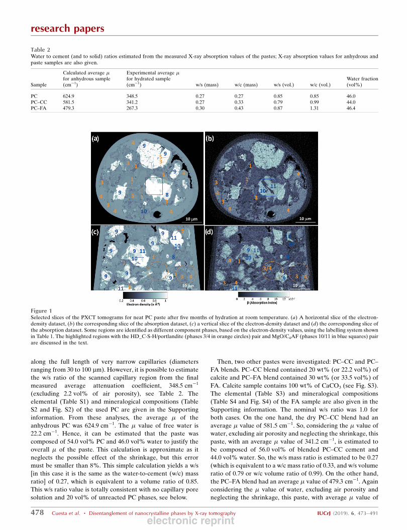
Figure 1Selected slices of the PXCT tomograms for neat PC paste after five months of hydration at room temperature. (a) A horizontal slice of the electron-density dataset, (b) the corresponding slice of the absorption dataset, (c) a vertical slice of the electron-density dataset and (d) the corresponding slice ofthe absorption dataset. Some regions are identified as different component phases, based on the electron-density values, using the labelling system shownin Table 1. The highlighted regions with the HD_C-S-H/portlandite (phases 3/4 in orange circles) pair and MgO/C4AF (phases 10/11 in blue squares) pairare discussed in the text.
electronic reprint
267.3 cm�1, is estimated to be composed of 53.6 vol% of
blended PC–FA cement and 46.4 vol% water. Hence, the w/s
mass ratio is estimated to be 0.30 (which is equivalent to a w/c
mass ratio of 0.43, and w/s volume ratio of 0.87 or w/c volume
ratio of 1.31). These values are summarized in Table 2.
3.3. PXCT electron densities and attenuation coefficients
PXCT yields two tomographic datasets: the 3D electron-
density distribution, ne(r), obtained from the phase projec-
tions, and the 3D distribution of the complex part of the
refraction index, �(r), obtained from the absorption projec-
tions. As expected, the resolution in the ne(r) dataset is better
in terms of noise and resolution than that in the �(r) one. The
3D spatial resolutions for the ne(r) datasets, determined by
FSC, were estimated to be 80, 56 and 59 nm (Fig. S5), for neat
PC, PC–CC and PC–FA blends, respectively. The 3D spatial
resolutions for the �(r) datasets were estimated to be around
250 nm.
3.3.1. Neat PC paste. Selected horizontal and vertical slices
for the ne(r) tomogram are shown in Figs. 1(a) and 1(c),
respectively. The corresponding slices in the �(r) tomogram
are shown in Figs. 1(b) and 1(d), respectively. Eight different
component phases were identified in the ne(r) tomogram
based on their electron densities (grey levels).
The qualitative analysis of Fig. 1 already gives valuable
information. The air porosity content (black regions within the
capillary) is very small. The grey level in the ne(r) tomogram is
lighter as the electron density for different phases increases.
AFt and C4AF being the components with lowest and highest
electron densities, respectively. As discussed above, the elec-
tron densities of C4AF and MgO are very close and they
cannot be distinguished in Figs. 1(a) and 1(c). However, as
shown in the blue square in Figs. 1(a) and 1(b), these
components can be easily differentiated in the (slightly
noisier) absorption tomogram. More importantly, C-S-H gel
and portlandite also have quite close electron-density values,
so they can hardly be discriminated in the electron-density
tomogram. However, these components can be readily
distinguished in the absorption tomogram, see the brown
circles in Figs. 1(c) and 1(d). PXCT tomograms revealed
different shapes for portlandite volumes as shown previously
by electron microscopy. They range from irregular forms with
sizes well above 15 mm to quite thin plaques (thicknesses
smaller than 0.5 mm) interspersed between C-S-H volumes, see
Fig. 1(d).
Ten random regions of particles were analysed for each
component phase to determine the electron densities, which
were then converted to mass densities by using equation (2)
and are given in Table 3. In general, the water content of C-S-
H is variable, hence the water content was determined as
explained below, and then the electron density could be
converted to volumetric mass density. It can be observed that
there is a very good agreement between both measured and
theoretical mass densities for crystalline component phases
(where the theoretical mass densities can be well defined). The
average relative error is lower than 1.5%. The electron
densities have also been obtained from the segmentation
volumes using Avizo software. A small systematic variation
between the measured and theoretical attenuation coefficients
has been observed in the three pastes. The origin of this
disagreement is not clear to us. However, as there are several
phases with well known attenuation coefficients (for instance,
the capillary, calcite and portlandite), we have used these
values to calculate the correction parameter which was 1.05
(i.e. 5%). Hence, all reported attenuation coefficients in this
work (for the three pastes) are determined from the complex
part or the refraction index datasets multiplied by the
correction factor 1.05.
An overall picture of the components can be obtained from
the electron-density histogram of a volume-of-interest (VOI)
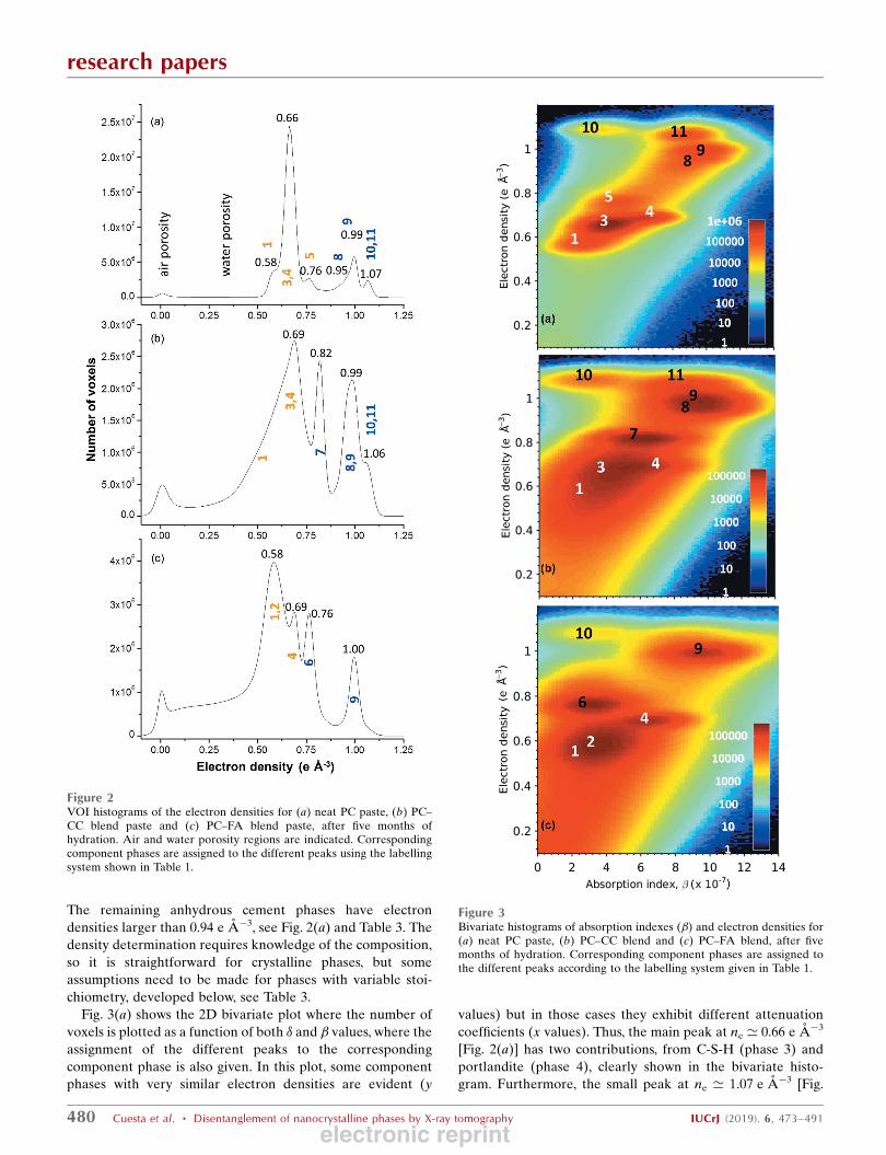
inside the capillary of about 1.6 � 104 mm3, see Fig. 2(a). The
shift in the air peak is caused by partial volume effects as the
computed region may contain liquid/solid phases below the
resolution of the data. The small peak at ne = 0.58 e A�3
corresponds to AFt, see Fig. 2(a) and Table 3. Fig. 2(a)
displays the strongest peak at ne ’ 0.66 e A�3. As it is shown
in Table 3 that peak is caused by two phases, one having ne ’0.65 e A�3 (C-S-H gel) and another with ne = 0.69 e A�3 (CH).
Furthermore, Fig. 2(a) displays a small peak at ne ’ 0.76 e A�3
(see also Table 3). It will be shown below that this peak
corresponds with Fe–Al siliceous hydrogarnet (Fe–Al–Si–Hg).
research papers
IUCrJ (2019). 6, 473–491 Cuesta et al. � Disentanglement of nanocrystalline phases by X-ray tomography 479
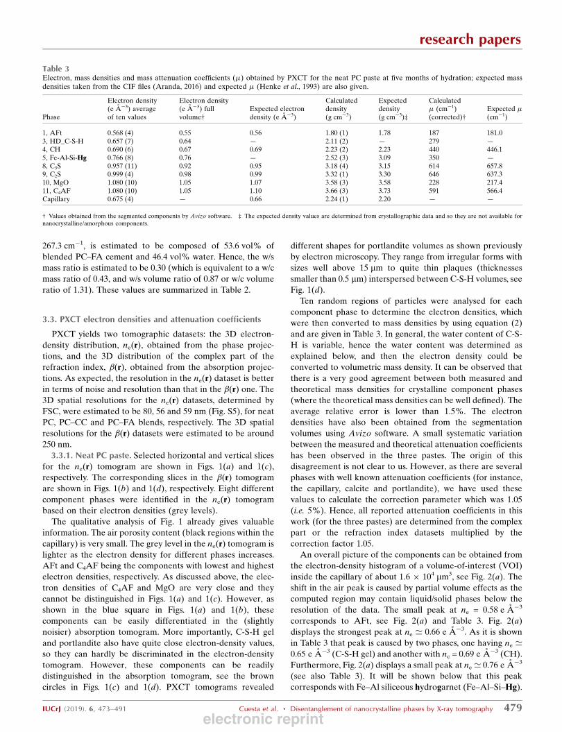
Table 3Electron, mass densities and mass attenuation coefficients (�) obtained by PXCT for the neat PC paste at five months of hydration; expected massdensities taken from the CIF files (Aranda, 2016) and expected � (Henke et al., 1993) are also given.
Phase
Electron density(e A�3) averageof ten values
Electron density(e A�3) fullvolume†
Expected electrondensity (e A�3)
Calculateddensity(g cm�3)
Expecteddensity(g cm�3)‡
Calculated� (cm�1)(corrected)†
Expected �(cm�1)
1, AFt 0.568 (4) 0.55 0.56 1.80 (1) 1.78 187 181.03, HD_C-S-H 0.657 (7) 0.64 — 2.11 (2) — 279 —4, CH 0.690 (6) 0.67 0.69 2.23 (2) 2.23 440 446.15, Fe-Al-Si-Hg 0.766 (8) 0.76 — 2.52 (3) 3.09 350 —8, C3S 0.957 (11) 0.92 0.95 3.18 (4) 3.15 614 657.89, C2S 0.999 (4) 0.98 0.99 3.32 (1) 3.30 646 637.310, MgO 1.080 (10) 1.05 1.07 3.58 (3) 3.58 228 217.411, C4AF 1.080 (10) 1.05 1.10 3.66 (3) 3.73 591 566.4Capillary 0.675 (4) — 0.66 2.24 (1) 2.20 — —
† Values obtained from the segmented components by Avizo software. ‡ The expected density values are determined from crystallographic data and so they are not available fornanocrystalline/amorphous components.
electronic reprint
The remaining anhydrous cement phases have electron
densities larger than 0.94 e A�3, see Fig. 2(a) and Table 3. The
density determination requires knowledge of the composition,
so it is straightforward for crystalline phases, but some
assumptions need to be made for phases with variable stoi-
chiometry, developed below, see Table 3.
Fig. 3(a) shows the 2D bivariate plot where the number of
voxels is plotted as a function of both � and � values, where the
assignment of the different peaks to the corresponding
component phase is also given. In this plot, some component
phases with very similar electron densities are evident (y
values) but in those cases they exhibit different attenuation
coefficients (x values). Thus, the main peak at ne ’ 0.66 e A�3
[Fig. 2(a)] has two contributions, from C-S-H (phase 3) and
portlandite (phase 4), clearly shown in the bivariate histo-
gram. Furthermore, the small peak at ne ’ 1.07 e A�3 [Fig.
research papers
480 Cuesta et al. � Disentanglement of nanocrystalline phases by X-ray tomography IUCrJ (2019). 6, 473–491
Figure 2VOI histograms of the electron densities for (a) neat PC paste, (b) PC–CC blend paste and (c) PC–FA blend paste, after five months ofhydration. Air and water porosity regions are indicated. Correspondingcomponent phases are assigned to the different peaks using the labellingsystem shown in Table 1.
Figure 3Bivariate histograms of absorption indexes (�) and electron densities for(a) neat PC paste, (b) PC–CC blend and (c) PC–FA blend, after fivemonths of hydration. Corresponding component phases are assigned tothe different peaks according to the labelling system given in Table 1.
electronic reprint
2(a)] has two contributions, from MgO (phase 10) and C4AF
(phase 11) as noticeable in Fig. 3(a).
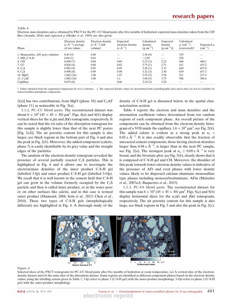
3.3.2. PC–CC blend paste. The reconstructed dataset was
about 6 � 104 (45 � 45 � 30) mm3. Figs. 4(a) and 4(b) display
vertical slices for the ne(r) and �(r) tomograms, respectively. It
can be noted that the s/n ratio of the absorption tomogram for
this sample is slightly lower than that of the neat PC pastes
[Fig. 1(d)]. The air porosity content for this sample is also
larger, see black regions in the bottom part of Fig. 4 and also
the peak in Fig. 2(b). Moreover, the added component (calcite,
phase 7) is easily identifiable by its grey value and the straight
edges of the particles.
The analysis of the electron-density tomogram revealed the
presence of several partially reacted C3S particles. This is
highlighted in Fig. 4 and it allows one to investigate the
electron/mass densities of the inner product C-S-H gel
(labelled 3-Ip) and outer product C-S-H gel (labelled 3-Op).
We recall that it is well known in the cement field that C-S-H
gel can grow in the volume formerly occupied by the C3S
particle and then is called inner product, or in the water pore
or on other surfaces like calcite, and in this case is termed
outer product (Diamond, 2004; Soin et al., 2013; Chen et al.,
2010). These two types of C-S-H gels (morphologically
different) are highlighted in Fig. 4. A thorough study of the
density of C-S-H gel is discussed below, in the spatial char-
acterization section.
Table 4 reports the electron and mass densities and the
attenuation coefficient values determined from ten random
regions of each component phase. An overall picture of the
components can be obtained from the electron-density histo-
gram of a VOI inside the capillary, 1.6 � 104 mm3, see Fig. 2(b).
The added calcite is evident as a strong peak at ne =
0.82 e A�3. It is also readily observable that the fraction of
unreacted cement components, those having electron densities
larger than 0.94 e A�3, is larger than in the neat PC sample,
see Fig. 2(a). The strongest peak at ne ’ 0.69 e A�3 is very
broad, and the bivariate plot, see Fig. 3(b), clearly shows that it
is composed of C-S-H gel and CH. Moreover, the shoulder of
this peak towards lower electron-density values is indicative of
the presence of AFt and even phases with lower density
values, likely to be dispersed calcium aluminate monosulfate
type phases including monocarboaluminate, AFm (Matschei
et al., 2007a,b; Baquerizo et al., 2015).
3.3.3. PC–FA blend paste. The reconstructed dataset for
this sample was 6 � 104 (45 � 45 � 30) mm3. Figs. 5(a) and 5(b)
display horizontal slices for the ne(r) and �(r) tomograms,
respectively. The air porosity content for this sample is also
large, see black regions in Fig. 5 and also the peak in Fig. 2(c).
research papers
IUCrJ (2019). 6, 473–491 Cuesta et al. � Disentanglement of nanocrystalline phases by X-ray tomography 481
Figure 4Selected slices of the PXCT tomograms for PC–CC blend paste after five months of hydration at room temperature. (a) A vertical slice of the electron-density dataset and (b) the same slice of the absorption dataset. Some regions are identified as different component phases based on the electron-densityvalues, using the labelling system given in Table 1. 3-Ip refers to phase 3 (C-S-H gel) with the inner-product morphology. 3-Op refers to phase 3 (C-S-Hgel) with the outer-product morphology.
Table 4Electron, mass densities and � obtained by PXCT for the PC–CC blend paste after five months of hydration; expected mass densities taken from the CIFfiles (Aranda, 2016) and expected � (Henke et al., 1993) are also given.
Phase
Electron density(e A�3) averageof ten values
Electron density(e A�3) fullvolume†
Expectedelectron density(e A�3)
Calculateddensity(g cm�3)
Expecteddensity(g cm�3)‡
Calculated� (cm�1)(corrected)†
Expected �(cm�1)
1, Monocarbo, AFt pore solution 0.45 (3) 0.48 — 1.36 (9) — 193 —3, HD_C-S-H 0.64 (1) 0.63 — �2.05 — 228 —4, CH 0.698 (7) 0.68 0.69 2.23 (2) 2.23 464 446.17, CC 0.826 (4) 0.80 0.82 2.75 (1) 2.71 411 415.28, C3S 0.963 (4) 0.93 0.95 3.20 (1) 3.15 649 657.89, C2S 0.998 (8) 0.99 0.99 3.32 (3) 3.30 639 637.310, MgO 1.062 (16) 1.06 1.07 3.52 (5) 3.58 211 217.411, C4AF 1.062 (16) 1.06 1.1 3.60 (5) 3.73 566 566.4Capillary 0.674 (6) — 0.66 2.24 (2) 2.20 — —
† Values obtained from the segmented components by Avizo software. ‡ The expected density values are determined from crystallographic data and so they are not no available fornanocrystalline/amorphous components.
electronic reprint
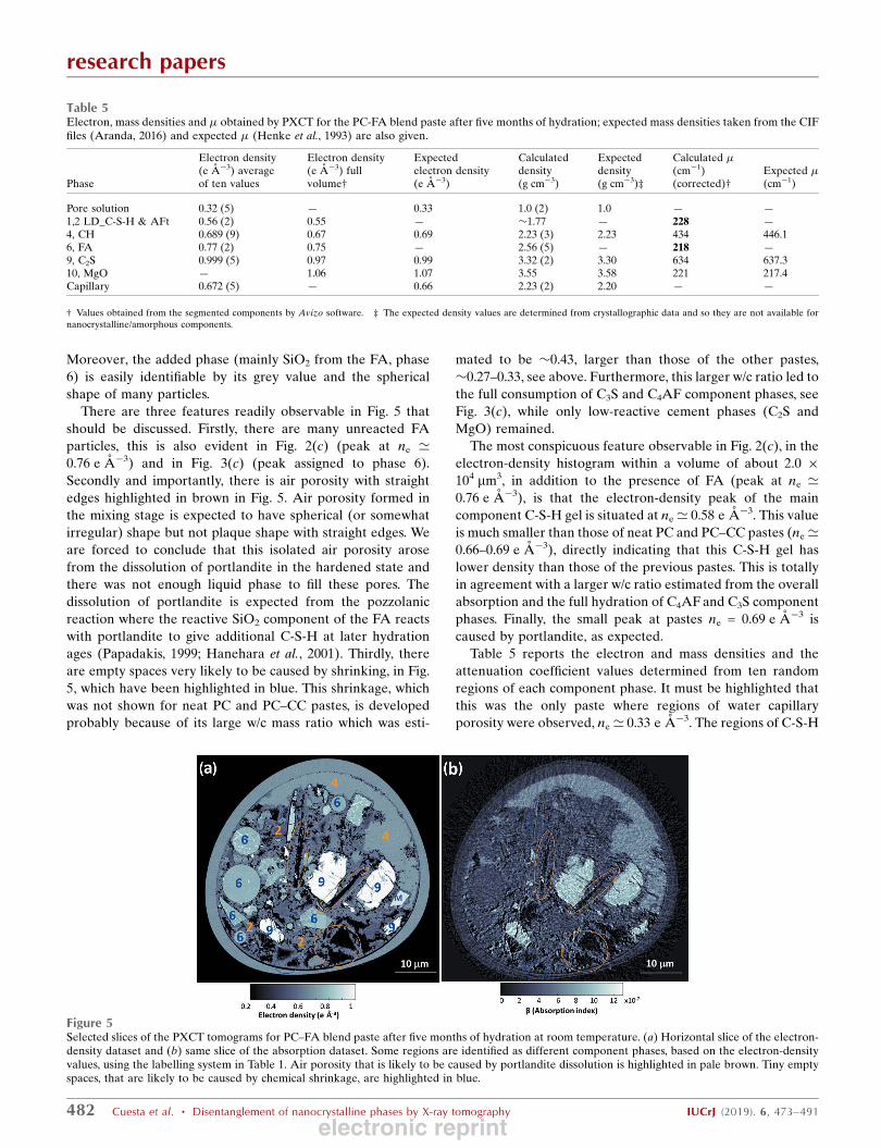
Moreover, the added phase (mainly SiO2 from the FA, phase
6) is easily identifiable by its grey value and the spherical
shape of many particles.
There are three features readily observable in Fig. 5 that
should be discussed. Firstly, there are many unreacted FA
particles, this is also evident in Fig. 2(c) (peak at ne ’0.76 e A�3) and in Fig. 3(c) (peak assigned to phase 6).
Secondly and importantly, there is air porosity with straight
edges highlighted in brown in Fig. 5. Air porosity formed in
the mixing stage is expected to have spherical (or somewhat
irregular) shape but not plaque shape with straight edges. We
are forced to conclude that this isolated air porosity arose
from the dissolution of portlandite in the hardened state and
there was not enough liquid phase to fill these pores. The
dissolution of portlandite is expected from the pozzolanic
reaction where the reactive SiO2 component of the FA reacts
with portlandite to give additional C-S-H at later hydration
ages (Papadakis, 1999; Hanehara et al., 2001). Thirdly, there
are empty spaces very likely to be caused by shrinking, in Fig.
5, which have been highlighted in blue. This shrinkage, which
was not shown for neat PC and PC–CC pastes, is developed
probably because of its large w/c mass ratio which was esti-
mated to be �0.43, larger than those of the other pastes,
�0.27–0.33, see above. Furthermore, this larger w/c ratio led to
the full consumption of C3S and C4AF component phases, see
Fig. 3(c), while only low-reactive cement phases (C2S and
MgO) remained.
The most conspicuous feature observable in Fig. 2(c), in the
electron-density histogram within a volume of about 2.0 �104 mm3, in addition to the presence of FA (peak at ne ’0.76 e A�3), is that the electron-density peak of the main
component C-S-H gel is situated at ne ’ 0.58 e A�3. This value
is much smaller than those of neat PC and PC–CC pastes (ne ’0.66–0.69 e A�3), directly indicating that this C-S-H gel has
lower density than those of the previous pastes. This is totally
in agreement with a larger w/c ratio estimated from the overall
absorption and the full hydration of C4AF and C3S component
phases. Finally, the small peak at pastes ne = 0.69 e A�3 is
caused by portlandite, as expected.
Table 5 reports the electron and mass densities and the
attenuation coefficient values determined from ten random
regions of each component phase. It must be highlighted that
this was the only paste where regions of water capillary
porosity were observed, ne ’ 0.33 e A�3. The regions of C-S-H
research papers
482 Cuesta et al. � Disentanglement of nanocrystalline phases by X-ray tomography IUCrJ (2019). 6, 473–491
Table 5Electron, mass densities and � obtained by PXCT for the PC-FA blend paste after five months of hydration; expected mass densities taken from the CIFfiles (Aranda, 2016) and expected � (Henke et al., 1993) are also given.
Phase
Electron density(e A�3) averageof ten values
Electron density(e A�3) fullvolume†
Expectedelectron density(e A�3)
Calculateddensity(g cm�3)
Expecteddensity(g cm�3)‡
Calculated �(cm�1)(corrected)†
Expected �(cm�1)
Pore solution 0.32 (5) — 0.33 1.0 (2) 1.0 — —1,2 LD_C-S-H & AFt 0.56 (2) 0.55 — �1.77 — 228 —4, CH 0.689 (9) 0.67 0.69 2.23 (3) 2.23 434 446.16, FA 0.77 (2) 0.75 — 2.56 (5) — 218 —9, C2S 0.999 (5) 0.97 0.99 3.32 (2) 3.30 634 637.310, MgO — 1.06 1.07 3.55 3.58 221 217.4Capillary 0.672 (5) — 0.66 2.23 (2) 2.20 — —
† Values obtained from the segmented components by Avizo software. ‡ The expected density values are determined from crystallographic data and so they are not available fornanocrystalline/amorphous components.
Figure 5Selected slices of the PXCT tomograms for PC–FA blend paste after five months of hydration at room temperature. (a) Horizontal slice of the electron-density dataset and (b) same slice of the absorption dataset. Some regions are identified as different component phases, based on the electron-densityvalues, using the labelling system in Table 1. Air porosity that is likely to be caused by portlandite dissolution is highlighted in pale brown. Tiny emptyspaces, that are likely to be caused by chemical shrinkage, are highlighted in blue.
electronic reprint
gel also contain ettringite and they could not be disentangled
as both electron density (ne ’ 0.57–0.59 e A�3) and attenua-
tion coefficient (� ’ 190–230 cm�1) values are too close.
3.4. Spatial characterization of selected component phases
A thorough analysis of the spatial distribution of the elec-
tron density for all component phases, hydrates and partly
reacted cement components, is out of the scope of this paper
and it will be the subject of a subsequent work. Here we focus
on key observations with implication for the nanocrystalline
component phase determination. This is the outstanding
contribution of PXCT to the cement hydration chemistry.
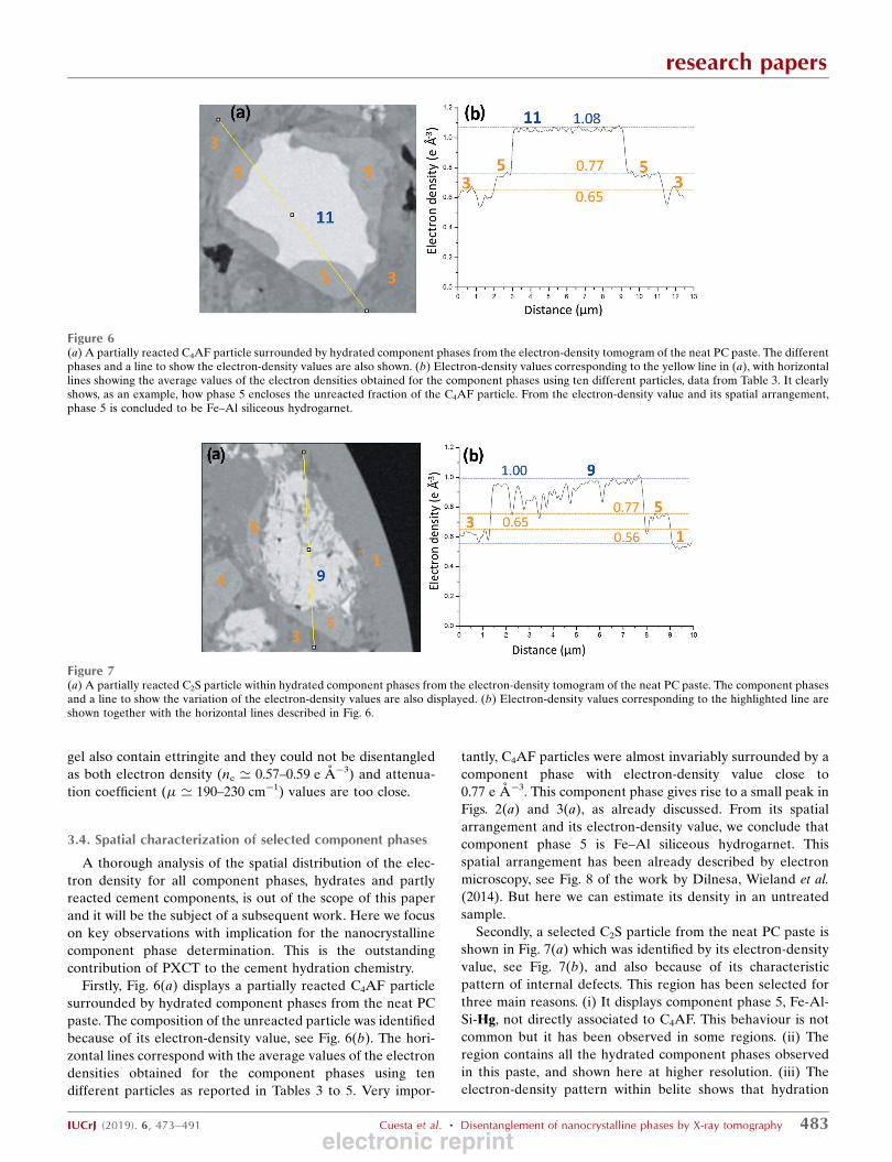
Firstly, Fig. 6(a) displays a partially reacted C4AF particle
surrounded by hydrated component phases from the neat PC
paste. The composition of the unreacted particle was identified
because of its electron-density value, see Fig. 6(b). The hori-
zontal lines correspond with the average values of the electron
densities obtained for the component phases using ten
different particles as reported in Tables 3 to 5. Very impor-
tantly, C4AF particles were almost invariably surrounded by a
component phase with electron-density value close to
0.77 e A�3. This component phase gives rise to a small peak in
Figs. 2(a) and 3(a), as already discussed. From its spatial
arrangement and its electron-density value, we conclude that
component phase 5 is Fe–Al siliceous hydrogarnet. This
spatial arrangement has been already described by electron
microscopy, see Fig. 8 of the work by Dilnesa, Wieland et al.
(2014). But here we can estimate its density in an untreated
sample.
Secondly, a selected C2S particle from the neat PC paste is
shown in Fig. 7(a) which was identified by its electron-density
value, see Fig. 7(b), and also because of its characteristic
pattern of internal defects. This region has been selected for
three main reasons. (i) It displays component phase 5, Fe-Al-
Si-Hg, not directly associated to C4AF. This behaviour is not
common but it has been observed in some regions. (ii) The
region contains all the hydrated component phases observed
in this paste, and shown here at higher resolution. (iii) The
electron-density pattern within belite shows that hydration
research papers
IUCrJ (2019). 6, 473–491 Cuesta et al. � Disentanglement of nanocrystalline phases by X-ray tomography 483
Figure 6(a) A partially reacted C4AF particle surrounded by hydrated component phases from the electron-density tomogram of the neat PC paste. The differentphases and a line to show the electron-density values are also shown. (b) Electron-density values corresponding to the yellow line in (a), with horizontallines showing the average values of the electron densities obtained for the component phases using ten different particles, data from Table 3. It clearlyshows, as an example, how phase 5 encloses the unreacted fraction of the C4AF particle. From the electron-density value and its spatial arrangement,phase 5 is concluded to be Fe–Al siliceous hydrogarnet.
Figure 7(a) A partially reacted C2S particle within hydrated component phases from the electron-density tomogram of the neat PC paste. The component phasesand a line to show the variation of the electron-density values are also displayed. (b) Electron-density values corresponding to the highlighted line areshown together with the horizontal lines described in Fig. 6.
electronic reprint
takes place along the defects, if they are connected to the
particle surfaces.
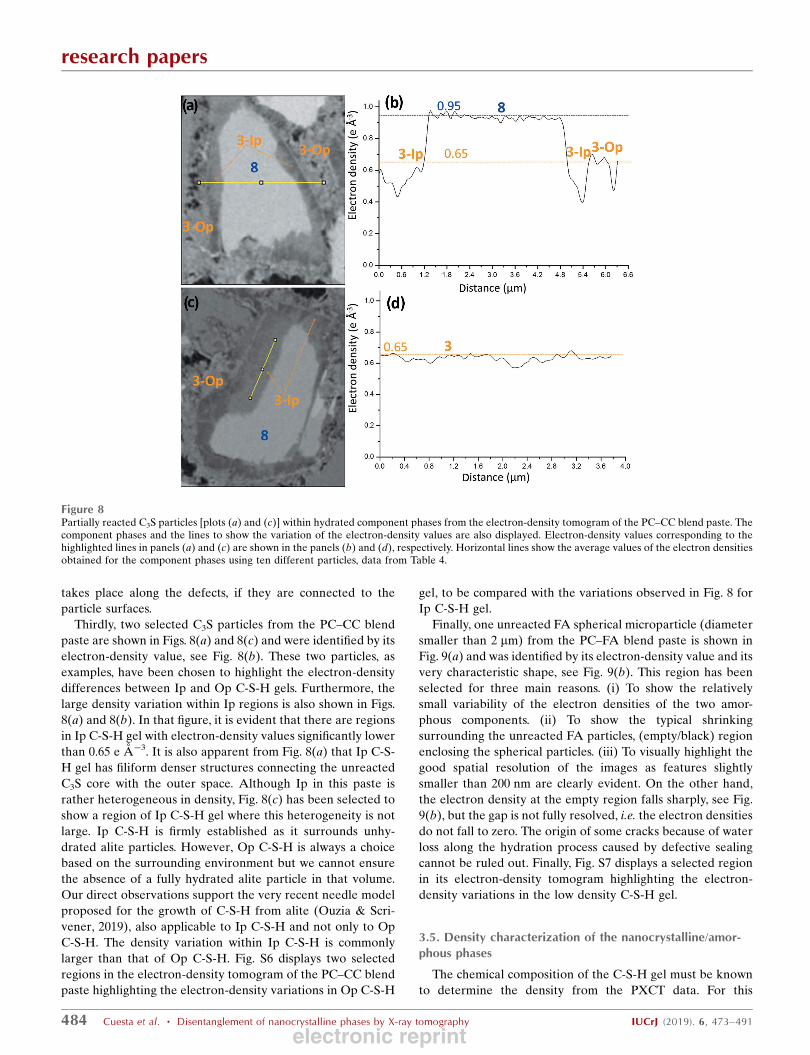
Thirdly, two selected C3S particles from the PC–CC blend
paste are shown in Figs. 8(a) and 8(c) and were identified by its
electron-density value, see Fig. 8(b). These two particles, as
examples, have been chosen to highlight the electron-density
differences between Ip and Op C-S-H gels. Furthermore, the
large density variation within Ip regions is also shown in Figs.
8(a) and 8(b). In that figure, it is evident that there are regions
in Ip C-S-H gel with electron-density values significantly lower
than 0.65 e A�3. It is also apparent from Fig. 8(a) that Ip C-S-
H gel has filiform denser structures connecting the unreacted
C3S core with the outer space. Although Ip in this paste is
rather heterogeneous in density, Fig. 8(c) has been selected to
show a region of Ip C-S-H gel where this heterogeneity is not
large. Ip C-S-H is firmly established as it surrounds unhy-
drated alite particles. However, Op C-S-H is always a choice
based on the surrounding environment but we cannot ensure
the absence of a fully hydrated alite particle in that volume.
Our direct observations support the very recent needle model
proposed for the growth of C-S-H from alite (Ouzia & Scri-
vener, 2019), also applicable to Ip C-S-H and not only to Op
C-S-H. The density variation within Ip C-S-H is commonly
larger than that of Op C-S-H. Fig. S6 displays two selected
regions in the electron-density tomogram of the PC–CC blend
paste highlighting the electron-density variations in Op C-S-H
gel, to be compared with the variations observed in Fig. 8 for
Ip C-S-H gel.
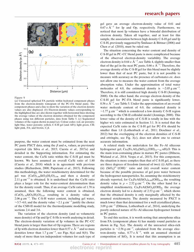
Finally, one unreacted FA spherical microparticle (diameter
smaller than 2 mm) from the PC–FA blend paste is shown in
Fig. 9(a) and was identified by its electron-density value and its
very characteristic shape, see Fig. 9(b). This region has been
selected for three main reasons. (i) To show the relatively
small variability of the electron densities of the two amor-
phous components. (ii) To show the typical shrinking
surrounding the unreacted FA particles, (empty/black) region
enclosing the spherical particles. (iii) To visually highlight the
good spatial resolution of the images as features slightly
smaller than 200 nm are clearly evident. On the other hand,
the electron density at the empty region falls sharply, see Fig.
9(b), but the gap is not fully resolved, i.e. the electron densities
do not fall to zero. The origin of some cracks because of water
loss along the hydration process caused by defective sealing
cannot be ruled out. Finally, Fig. S7 displays a selected region
in its electron-density tomogram highlighting the electron-
density variations in the low density C-S-H gel.
3.5. Density characterization of the nanocrystalline/amor-phous phases
The chemical composition of the C-S-H gel must be known
to determine the density from the PXCT data. For this
research papers
484 Cuesta et al. � Disentanglement of nanocrystalline phases by X-ray tomography IUCrJ (2019). 6, 473–491
Figure 8Partially reacted C3S particles [plots (a) and (c)] within hydrated component phases from the electron-density tomogram of the PC–CC blend paste. Thecomponent phases and the lines to show the variation of the electron-density values are also displayed. Electron-density values corresponding to thehighlighted lines in panels (a) and (c) are shown in the panels (b) and (d), respectively. Horizontal lines show the average values of the electron densitiesobtained for the component phases using ten different particles, data from Table 4.
electronic reprint
purpose, the water content must be estimated from the neat
PC paste PXCT data, using the � and ne values, as previously
reported (da Silva et al., 2015; Cuesta et al., 2017a) and
detailed in the Supporting information. For estimating the
water content, the Ca/Si ratio within the C-S-H gel must be
known. We have assumed an overall Ca/Si ratio of 1.80
(Cuesta et al., 2018) which is in agreement with previous
studies (Richardson, 2008; Papatzani et al., 2015). Following
this methodology, the water stoichiometry determined for the
gel was (CaO)1.80SiO2(H2O)3.96 and then a density of
2.11 g cm�3 is obtained. It is underlined that the Ca/Si ratio
plays a larger role for the water-content determination than
for the density result. Thus, if an average Ca/Si ratio of 1.70 is
assumed, then the following water content is obtained,
(CaO)1.70SiO2(H2O)3.65 resulting in a density value of
2.06 g cm�3. The C-S-H water content, including gel water,
�3.7–4.0, and the density value �2.1 g cm�3 justify the choice
of the CSH-II model for the thermodynamic modelling study,
sections 2.4 and 3.6.
The variation of the electron density (and so volumetric
mass density) of Op and Ip C-S-Hs is worth analysing in detail.
The electron-density variation of Ip volumes in the PC–CC
blend paste is larger than that of Op regions. There are regions
of Ip with electron densities lower than 0.57 e A�3 and so mass
densities lower than 1.7 g cm�3, see Figs. 8(a) and 8(b). The
study of more than ten independent volumes for each type of
gel gave an average electron-density value of 0.61 and
0.67 e A�3 for Ip and Op, respectively. Furthermore, we
noticed that most Ip volumes have a bimodal distribution of
electron density. Taken all together, and at least for this
sample, the association between high density C-S-H gel and Ip
C-S-H, previously suggested by Smilauer & Bittnar (2006) and
Chen et al. (2010), must be ruled out.
The situation concerning the water content and density of
C-S-H gel in PC–CC blend paste is more complicated because
of the observed electron-density variability. The average
electron density is 0.64 e A�3, see Table 4, slightly smaller than
that of the gel in the neat PC paste, 0.66 e A�3. Therefore, the
average density of the C-S-H gel for this blend must be slightly
lower than that of neat PC paste, but it is not possible to
measure with accuracy as the presence of carbonates etc. does
not allow one to measure the water content from the average
absorption value. Under the approximation of total water
molecules of 4.0, the estimated density is �2.05 g cm�3.
Therefore, it is still considered high density C-S-H (Jennings,
2008). On the other hand, the average electron density of the
C-S-H gel for PC–FA blend paste is significantly lower,
0.56 e A�3, see Table 5. Under the approximation of an overall
water molecule content of 6.0, the estimated density is
�1.77 g cm�3 which is considered a low density C-S-H region
according to the CM-II colloidal model (Jennings, 2008). This
lower value of the density of C-S-H is totally in line with the
higher w/c ratio estimated in Section 3.1. It is noted that the
expected Ca/Si ratio in the C-S-H gel for PC–FA should be
smaller than 1.8 (Lothenbach et al., 2011; Deschner et al.,
2012) but the overlapping of the electron densities of C-S-H
and ettringite, see Fig. 3(c), does not allow one to extract
accurate information.
A related study was undertaken for the Fe–Al siliceous
hydrogarnet gel, Ca3(Fe,Al)2(SiO4)y(OH)12�4y�nH2O. This is
the main iron-containing phase in mature PC pastes (Dilnesa,
Wieland et al., 2014; Vespa et al., 2015). For this component,
the situation is more complex than that of C-S-H gel, as there
are three degrees of freedom (instead of two): (i) Al/Fe ratio,
(ii) (SiO4)4�/(OH)� ratio and (iii) overall water content
because of the possible presence of gel pore water between
the hydrogarnet nanoparticles. So, assuming the stoichiometry
already reported, for Ca3FeAl(SiO4)0.84(OH)8.64 the resulting
density value is � = 2.52 g cm�3. On the other hand for a
simplified stoichiometry, Ca3FeAl(SiO4)(OH)8, the average
electron density led to a density of 2.53 g cm�3, which shows
that the obtained density is only marginally affected by the
assumed stoichiometry. The density measured by PXCT is
much lower than that determined for a well crystallized phase,
3.09 g cm�3 (Dilnesa, Lothenbach et al., 2014), underlying the
poorly ordered nature of Fe–Al siliceous hydrogarnet formed
in PC pastes.
To end this section, it is worth noting that amorphous silica
from FA (component phase 6) has mainly round particles as
shown in Fig. 5(a). The density of the unreacted silica-rich
particles is �2.56 g cm�3, calculated from the average elec-
tron-density value, 0.77 e A�3, with an assumed chemical
composition of SiO2. It is noted that this assumption is an
research papers
IUCrJ (2019). 6, 473–491 Cuesta et al. � Disentanglement of nanocrystalline phases by X-ray tomography 485
Figure 9(a) Unreacted spherical FA particle within hydrated component phasesfrom the electron-density tomogram of the PC–FA blend paste. Thecomponent phases and a line to show the variation of the electron densityvalues are also displayed. (b) Electron-density values corresponding tothe highlighted line are also shown together with horizontal lines showingthe average values of the electron densities obtained for the componentphases using ten different particles, data from Table 5. (c) Segmentedvolumes of the region shown in panel (a). Colour codes: red, air porosity;light blue, water porosity; yellow, C-S-H gel (and AFt); light green, CH;light pink, FA; and brown, C2S.
electronic reprint
approximation because of the large Al2O3 content of the FA,
26.4 wt%, see Table S3. The density of FA depends upon its
composition. Reported average density values of F-class and
C-class are 2.38 and 2.65 g cm�3, respectively (Kosmatka et al.,
1996). It is natural to deduce that lower density silica particles
are more reactive for the pozzolanic reaction, and the
unreacted fraction is that mainly composed by high density
particles. For the sake of completeness, we also give here the
density values of the room pressure crystalline SiO2 poly-
morphs quartz, cristobalite and tridymite, which are 2.65, 2.32
and 2.31 g cm�3, respectively (Chatterton & Cross, 1972).
3.6. PXCT tomogram segmentation: quantitative componentphase analysis
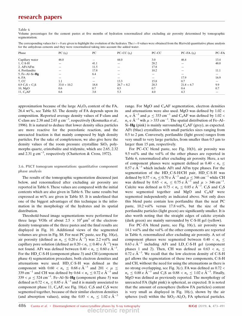
The results of the tomographic segmentation discussed just
below, and renormalized after excluding air porosity are
reported in Table 6. These values are compared with the initial
contents which are also given in Table 6. The same results but
expressed as wt% are given in Table S5. It is underlined that
one of the biggest advantages of this technique is the infor-
mation in the morphology of the hydrates and its spatial
distribution.
Threshold-based image segmentations were performed for
three large VOIs of about 2.5 � 104 mm3 of the electron-
density tomograms of the three pastes and the final results are
displayed in Fig. 10. Additional views of the segmented
volumes are given in Fig. S8. For neat PC paste, see Fig. 10(a),
air porosity (defined as ne � 0.20 e A�3) was 2.2 vol% and
capillary pore solution (defined as 0.20 < ne � 0.40 e A�3) was
not found. AFt was defined between 0.40 < ne � 0.60 e A�3.
For the HD_C-S-H (component phase 3) and CH (component
phase 4) segmentation procedure, both electron densities and
attenuations were used. HD_C-S-H was defined as the
component with 0.60 < ne � 0.68 e A�3 and 201 < � �339 cm�1 and CH was defined by 0.64 < ne � 0.72 e A�3 and
339 < � � 524 cm�1. Fe–Al–Si–Hg (component phase 5) was
defined as 0.72 < ne � 0.85 e A�3 and it is mainly associated to
component phase 11, C4AF, see Fig. 10(a). C3S and C2S were
segmented together, because of their similar electron densities
(and absorption values), using the 0.85 < ne � 1.02 e A�3
range. For MgO and C4AF segmentation, electron densities
and attenuations were also used. MgO was defined by 1.02 <
ne e A�3 and � � 333 cm�1 and C4AF was defined by 1.02 <
ne e A�3 wih � > 333 cm�1. The spatial distribution of Fe–Al–
Si–Hg (pink) is mainly surrounding C4AF (grey), as expected.
AFt (blue) crystallizes with small particles sizes ranging from
0.5 to 2 mm. Conversely, portlandite (light green) ranges from
very small to very large particles, from smaller than 0.5 mm to
larger than 15 mm, respectively.
For PC–CC blend paste, see Fig. 10(b), air porosity was
9.5 vol% and the vol% of the other phases are reported in
Table 6, renormalized after excluding air porosity. Here, a set
of component phases were segment defined as 0.40 < ne �0.57 e A�3 which include AFt and AFm type phases. For the
segmentation of the HD_C-S-H/CH pair, HD_C-S-H was
defined by 0.57 < ne � 0.70 e A�3 and � � 346 cm�1 while CH
was defined by 0.65 < ne � 0.75 e A�3 and � > 346 cm�1.
Calcite was defined as 0.75 < ne � 0.85 e A�3. C3S and C2S
were segmented together and MgO and C4AF were
segmented independently as indicated above. Not only does
this blend paste contain less portlandite than the neat PC
paste, 10.2 vol% versus 17.8 vol%, but the size of the
portlandite particles (light green) are significantly smaller. It is
also worth noting that the straight edges of calcite crystals
(dark green) are mainly surrounded by C-S-H gel (yellow).
For PC–FA blend paste, see Fig. 10(c), air porosity was
14.1 vol% and the vol% of the other components are reported
in Table 6, renormalized after excluding air porosity. A set of
component phases were segmented between 0.40 < ne �0.63 e A�3 including AFt and LD_C-S-H gel (component
phases 1 and 2). Then, CH was defined as 0.63 < ne �0.72 e A�3. We recall that the low electron density of C-S-H
gel allows the segmentation of these two components, C-S-H
and CH, without the need for using the attenuations as there is
no strong overlapping, see Fig. 3(c). FA was defined as 0.72 <
ne � 0.88 e A�3 and C2S as 0.88 < ne � 1.02 e A�3. Finally,
MgO was defined as previously reported. The morphology of
unreacted FA (light pink) is spherical, as expected. It is noted
that the amount of cenosphere (hollow FA particles) content
is very small as displayed in Fig. 10(c), shown by the air
spheres (red) within the SiO2–Al2O3 FA spherical particles.
research papers
486 Cuesta et al. � Disentanglement of nanocrystalline phases by X-ray tomography IUCrJ (2019). 6, 473–491
Table 6Volume percentages for the cement pastes at five months of hydration renormalized after excluding air porosity determined by tomographicsegmentation.
The corresponding values for t = 0 are given to highlight the evolution of the hydrates. The t = 0 values were obtained from the Rietveld quantitative phase analysisfor the anhydrous cements and they were renormalized taking into account the added water.
Phase PC (t0) PC PC–CC (t0) PC–CC PC–FA (t0) PC–FA
Capillary water 46.0 — 44.0 3.0 46.4 13.41, C-S-H — 41.1 — 28.2 — 48.02, AFt/AFm — 11.5 — 17.8 —4, Portlandite — 17.8 — 10.2 — 11.15, Fe–Al–Si–Hg — 6.4 — — — —6, FA — — — — 17.9 16.97, CC 1.1 — 13.3 15.8 0.7 —8,9 C3S + C2S 33.0 + 10.2 18.8 26.7 + 8.2 20.3 21.8 + 6.7 9.910, MgO 0.6 0.7 0.5 0.7 0.4 0.711, C4AF 6.6 3.8 5.3 4.0 4.3 —
electronic reprint
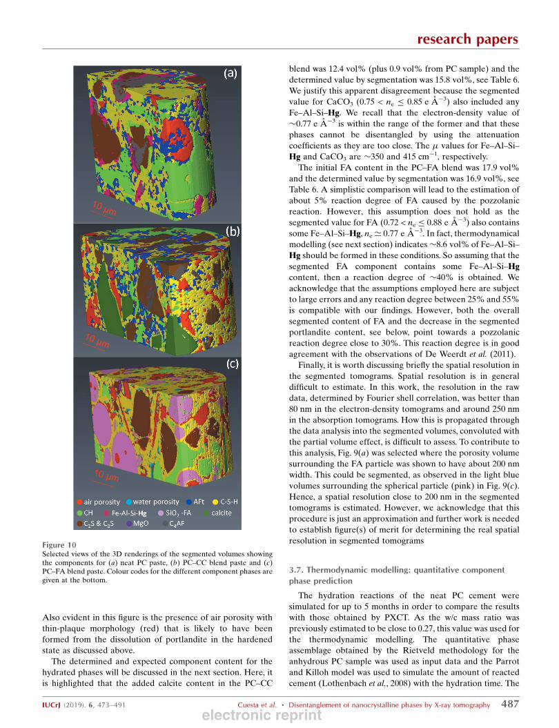
Also evident in this figure is the presence of air porosity with
thin-plaque morphology (red) that is likely to have been
formed from the dissolution of portlandite in the hardened
state as discussed above.
The determined and expected component content for the
hydrated phases will be discussed in the next section. Here, it
is highlighted that the added calcite content in the PC–CC
blend was 12.4 vol% (plus 0.9 vol% from PC sample) and the
determined value by segmentation was 15.8 vol%, see Table 6.
We justify this apparent disagreement because the segmented
value for CaCO3 (0.75 < ne � 0.85 e A�3) also included any
Fe–Al–Si–Hg. We recall that the electron-density value of
�0.77 e A�3 is within the range of the former and that these
phases cannot be disentangled by using the attenuation
coefficients as they are too close. The � values for Fe–Al–Si–
Hg and CaCO3 are �350 and 415 cm�1, respectively.
The initial FA content in the PC–FA blend was 17.9 vol%
and the determined value by segmentation was 16.9 vol%, see
Table 6. A simplistic comparison will lead to the estimation of
about 5% reaction degree of FA caused by the pozzolanic
reaction. However, this assumption does not hold as the
segmented value for FA (0.72 < ne � 0.88 e A�3) also contains
some Fe–Al–Si–Hg, ne ’ 0.77 e A�3. In fact, thermodynamical
modelling (see next section) indicates �8.6 vol% of Fe–Al–Si–
Hg should be formed in these conditions. So assuming that the
segmented FA component contains some Fe–Al–Si–Hg
content, then a reaction degree of �40% is obtained. We
acknowledge that the assumptions employed here are subject
to large errors and any reaction degree between 25% and 55%
is compatible with our findings. However, both the overall
segmented content of FA and the decrease in the segmented
portlandite content, see below, point towards a pozzolanic
reaction degree close to 30%. This reaction degree is in good
agreement with the observations of De Weerdt et al. (2011).
Finally, it is worth discussing briefly the spatial resolution in
the segmented tomograms. Spatial resolution is in general
difficult to estimate. In this work, the resolution in the raw
data, determined by Fourier shell correlation, was better than
80 nm in the electron-density tomograms and around 250 nm
in the absorption tomograms. How this is propagated through
the data analysis into the segmented volumes, convoluted with
the partial volume effect, is difficult to assess. To contribute to
this analysis, Fig. 9(a) was selected where the porosity volume
surrounding the FA particle was shown to have about 200 nm
width. This could be segmented, as observed in the light blue
volumes surrounding the spherical particle (pink) in Fig. 9(c).
Hence, a spatial resolution close to 200 nm in the segmented
tomograms is estimated. However, we acknowledge that this
procedure is just an approximation and further work is needed
to establish figure(s) of merit for determining the real spatial
resolution in segmented tomograms
3.7. Thermodynamic modelling: quantitative componentphase prediction
The hydration reactions of the neat PC cement were
simulated for up to 5 months in order to compare the results
with those obtained by PXCT. As the w/c mass ratio was
previously estimated to be close to 0.27, this value was used for
the thermodynamic modelling. The quantitative phase
assemblage obtained by the Rietveld methodology for the
anhydrous PC sample was used as input data and the Parrot
and Killoh model was used to simulate the amount of reacted
cement (Lothenbach et al., 2008) with the hydration time. The
research papers
IUCrJ (2019). 6, 473–491 Cuesta et al. � Disentanglement of nanocrystalline phases by X-ray tomography 487
Figure 10Selected views of the 3D renderings of the segmented volumes showingthe components for (a) neat PC paste, (b) PC–CC blend paste and (c)PC–FA blend paste. Colour codes for the different component phases aregiven at the bottom.
electronic reprint
hydration evolution was followed for up to 5 months, see Fig.
S9. It is noted that this comparison should be exercised with
care as some approximations and systematic errors can have a
role to play. Firstly, the w/s ratio estimated by PXCT is subject
to error and it is not necessarily constant along such thin
capillaries. Secondly, the ultrasound treatment can alter the
anhydrous phase assemblage. Thirdly, the segmentation
procedure groups all the component phases with a similar
electron density (and attenuation value). Finally, the ther-
modynamic modelling also contains approximations. In any
case, the comparison is given for a semi-quantitative valida-
tion. Hence, Table 7 shows the phase assemblage, in volume
percentage, for the neat PC cement (including the added
water) and that for the hydrated PC cement after 5 months of
hydration obtained by thermodynamic modelling and by
PXCT (excluding air porosity). The agreement between both
methodologies is reasonable considering the complexity of the
sample. The thermodynamic modelling analysis shows that the
reaction degree is slightly larger than that observed by PXCT,
as there are a fewer number of anhydrous components after 5
months. The pore solution content predicted in the thermo-
dynamic modelling is very low which is in agreement with the
absence of porosity found in the PXCT study. Moreover, the
precipitation of C-S-H and CH matched, within the margin of
error, the experimental results obtained by PXCT. In addition,
it is worth mentioning the relatively good agreement for Fe–
Al siliceous content. Finally, the largest disagreement is
related to the content of ettringite. This could be because of a
number or reasons including that thermodynamic modelling
assumes all sulfates crystallize as ettringite but this anion can
be partly incorporated into other phases.
The same type of study was performed for the PC–CC blend
paste. The w/s mass ratio of the PXCT studied region was 0.27.
Table 8 shows the phase assemblage, in volume percentage, for
the anhydrous PC–CC blend and for the hydrated sample after
5 months of hydration obtained by thermodynamic modelling
and by PXCT (excluding air porosity). Fig. S10 displays the
evolution of the phase assemblage for this paste obtained by
thermodynamic modelling. The comparison of the data shown
in Table 8 indicates that the fraction of unreacted phases
measured by PXCT was larger than that calculated by
modelling. Furthermore, greater pore solution content was
calculated by modelling than found experimentally. This can
be explained by a (slightly) larger w/s ratio than that estimated
in Section 3.2 and also by a larger degree of reaction deduced
from the Parrot and Killoh model. It is worth mentioning that
the measured calcite content by PXCT was larger than the
initial value, 15.8 vol% versus 13.3 vol%, because it also
contains the amount of formed Fe–Al–Si–Hg, see Table 8. The
agreement between the modelled and determined C-S-H
contents is very satisfactory. However, the portlandite content
determined by PXCT was lower than that modelled and also
than that expected from a calcite dilution of the neat PC study
shown above. This result requires further investigation or
confirmation.
For the PC–FA blend paste, the w/s ratio of the studied
region was 0.30. The phase assemblage’s evolution for the
paste obtained by thermodynamic modelling is shown in Fig.
S11, and Table 9 reports the phase assemblages modelled after
5 months of hydration and measured by PXCT (excluding air
porosity). The measured unreacted FA content by PXCT was
16.9 vol% larger than the initial value because it also contains
the amount of Fe–Al–Si–Hg formed. Chiefly, portlandite
content measured by PXCT, 11.1 vol%, is lower than the value
determined for the neat PC shown above, �18 vol%, and after
dilution with the added FA, �14 vol%. This is indirect proof
of a pozzolanic reaction which is even clearer when consid-
ering that the unreacted fraction of Portland cement is lower
in the PC–FA blend. However, the PXCT determined value,
11.1 vol%, is larger than the modelled value, 5.8 vol%, which
is justified by the set of approximations used in both
approaches.
4. Conclusions
Despite the relatively low spatial resolution, �250 nm, and s/n
ratio in the absorption tomograms compared with the elec-
research papers
488 Cuesta et al. � Disentanglement of nanocrystalline phases by X-ray tomography IUCrJ (2019). 6, 473–491
Table 7Phase assemblage for the neat PC paste and after five months ofhydration (by thermodynamic simulation with GEMs and by PXCT).
PhaseVol % (initial)with water Vol % (GEMs) Vol % (PXCT)
C3S 33.0 5.4 18.8C2S 10.2 6.3C4AF 6.6 3.8 3.8MgO 0.6 0.4 0.7C3A† 1.5 0.4 —Bass 1.0 — —CaCO3 1.1 0.9 —Fe–Al–Si–Hg — 4.0 6.4Portlandite — 20.1 17.8C-S-H gel — 35.3 41.1Hydrotalcite
(2.01 g cm�3)— 1.3 —‡
AFt — 18.6 11.5Pore solution 46.0 3.6 0
† C3A correspond to Ca3Al2O6 ‡ Hydrotalcite, if present, could not be independentlysegmented as its electron density and attenuation values are too close to those of C-S-Hgel.
Table 8Phase assemblage for the PC–CC blend paste and after five months ofhydration (by thermodynamic simulation with GEMs and by PXCT).
PhaseVol % (initial)with water Vol % (GEMs) Vol % (PXCT)
C3S 26.7 3.0 20.3C2S 8.2 4.1C4AF 5.3 2.3 4.0MgO 0.5 0.4 0.7C3A 1.2 0.2 —Bass 0.8 — —CaCO3 13.3 13.8 15.8Fe–Al–Si–Hg — 4.1 —†Portlandite — 17.0 10.2C-S-H — 29.2 28.2Hydrotalcite — 1.2 —AFt — 14.7 17.8Pore solution 44.0 10.1 3.0
† Fe–Al–Si–Hg could not be independently segmented as its electron density andattenuation values are too close to those of calcium carbonate.
electronic reprint
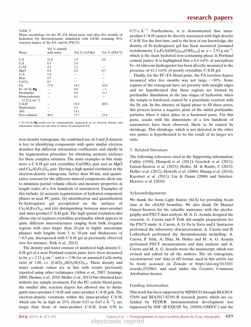
tron-density tomograms, the combined use of � and � datasets
is key to identifying components with quite similar electron
densities but different attenuation coefficients, and chiefly in
the segmentation procedure for obtaining accurate analyses
for these complex mixtures. The main examples in this study
were a C-S-H gel and crystalline Ca(OH)2 pair and an MgO
and Ca4Al2Fe2O10 pair. Having a high spatial resolution in the
electron-density tomograms, better than 80 nm, and quanti-
tative contrast for the different mineral components allow one
to minimize partial volume effects and measure properties at
length scales of a few hundreds of nanometres. Examples of
this include: (i) accurate segmentation of hydrated component
phases in neat PC paste; (ii) identification and quantification
Fe-hydrogarnet gel precipitated on the surfaces of
Ca4Al2Fe2O10; and (iii) distinguishing between inner-product
and outer-product C-S-H gels. The high spatial resolution also
allows one to segment crystalline portlandite which appears in
quite different microstructures ranging from bulk irregular
regions with sizes larger than 20 mm to highly anisotropic
plaques with lengths from 5 to 10 mm and thicknesses of
�0.5 mm, interspersed with C-S-H gel as previously observed
(see for instance, Trtik et al., 2012).
The density and water content of unaltered high-density C-
S-H gel of a neat Portland cement paste have been measured
to be � = 2.11 g cm�3 and n = 3.96 for an assumed Ca/Si molar
ratio of 1.80, i.e. (CaO)1.8SiO2(H2O)4.0. These density and
water content values are in line with results previously
reported using other techniques (Allen et al., 2007; Jennings,
2008; Thomas et al., 2010; Muller et al., 2013) but obtained here
without any sample treatment. For the PC–calcite blend paste,
the smaller alite reaction degree has allowed one to distin-
guish inner-product C-S-H and outer-product C-S-H gels. The
electron-density variations within the inner-product C-S-H,
which can be as high as 25% (from 0.53 to 0.67 e A�3), are
larger than those of outer-product C-S-H, from 0.59 to
0.73 e A�3. Furthermore, it is demonstrated that inner-
product C-S-H cannot be directly associated with high-density
C-S-H. For the first time, and to the best of our knowledge, the
density of Fe-hydrogarnet gel has been measured [assumed
stoichiometry Ca3FeAl(SiO4)0.84(OH)8.64] as � = 2.52 g cm�3,
which is the main hydrated iron-containing phase in Portland
cement pastes. It is highlighted that a 6.4 vol% of amorphous
Fe–Al siliceous hydrogarnet has been directly measured in the
presence of 41.1 vol% of poorly crystalline C-S-H gel.
Finally, for the PC–FA blend paste, the FA reaction degree
measured after five months was not large, �30%. Some
regions of the tomogram have air porosity with straight edges
and we hypothesized that these regions are formed by
portlandite dissolution at the late stages of hydration, when
the sample is hardened, caused by a pozzolanic reaction with
the fly ash. In the absence of liquid phase to fill these pores,
this process leaves a negative print of the initial portlandite
particles when it takes place in a hardened paste. For this
paste, cracks with the dimensions of a few hundreds of
nanometres have been observed, likely to be caused by
shrinkage. This shrinkage, which is not detected in the other
two pastes, is hypothesized to be the result of its larger w/c
ratio.
5. Related literature
The following references cited in the Supporting information:
Cullity (1956); Dinapoli et al. (2011); Gorelick et al. (2011);
Guizar-Sicairos et al. (2015); Holler, M. & Raabe, J. (2015);
Holler et al. (2012); Howells et al. (2009); Huang et al. (2014);
Kaestner et al. (2011); Liu & Daum (2008) and Sanchez-
Herrero et al. (2016).
Acknowledgements
We thank the Swiss Light Source (SLS) for providing beam
time at the cSAXS beamline. We also thank Dr Manuel
Guizar-Sicairos for his valuable assistance with the ptycho-
graphy and PXCT data analysis. M. A. G. Aranda designed the
research; A. Cuesta and P. Trtik did sample preparations for
the PXCT study; A. Cuesta, A. G. De la Torre and I. Santacruz
performed the laboratory characterization; A. Cuesta and B.
Lothenbach performed the thermodynamic modelling; A.
Cuesta, P. Trtik, A. Diaz, M. Holler and M. A. G. Aranda
performed PXCT measurements and data analysis; and A.
Cuesta and M. A. G. Aranda wrote the manuscript, which was
revised and edited by all the authors. The six tomograms,
reconstructed ‘raw’ data in tiff format, used in this article can
be freely accessed on Zenodo at https://doi.org/10.5281/
zenodo.2533863, and used under the Creative Commons
Attribution licence.
Funding information
This work has been supported by MINECO through BIA2014-
57658 and BIA2017-82391-R research grants, which are co-
funded by FEDER. Instrumentation development was
supported by SNF (R’EQUIP, No. 145056,‘OMNY’) and the
research papers
IUCrJ (2019). 6, 473–491 Cuesta et al. � Disentanglement of nanocrystalline phases by X-ray tomography 489
Table 9Phase assemblage for the PC–FA blend paste and after five months ofhydration (by thermodynamic simulation with GEMs assuming 30%reaction degree of the FA, and by PXCT).
PhaseVol % (initial)with water Vol % (GEMs) Vol % (PXCT)
C3S 21.8 1.5 9.9C2S 6.7 2.4C4AF 4.3 1.2 —MgO 0.4 0.2 0.7C3A 1.0 — —Bass 0.7 — —CaCO3 0.7 — —FA 17.9 14.2 16.9Fe–Al–Si–Hg — 8.6 —†Portlandite — 5.8 11.1Monocarbonate
(2.22 g cm�3)— 4.1 —
C-S-H — 35.8 48.0Hydrotalcite — 1.5AFt — 13.1Pore solution 46.4 11.7 13.4
† Fe–Al–Si–Hg could not be independently segmented as its electron density andattenuation values are too close to those of (unreacted) FA.
electronic reprint
Competence Centre for Materials Science and Technology
(CCMX) of the ETH-Board, Switzerland.
References
Abramoff, M. D., Magalhaes, P. J. & Ram, S. J. (2004). BiophotonicsInt. 11, 36–42.
Allen, A. J., Thomas, J. J. & Jennings, H. M. (2007). Nat. Mater. 6, 311–316.
Andalibi, M. R., Kumar, A., Srinivasan, B., Bowen, P., Scrivener, K.,Ludwig, C. & Testino, A. (2018). J. Mater. Chem. A, 6, 363–373.
Aranda, M. A. G. (2016). Crystallogr. Rev. 22, 150–196.Artioli, G., Cerulli, T., Cruciani, G., Dalconi, M. C., Ferrari, G.,
Parisatto, M., Rack, A. & Tucoulou, R. (2010). Anal. Bioanal.Chem. 397, 2131–2136.
Artioli, G., Valentini, L., Voltolini, M., Dalconi, M. C., Ferrari, G. &Russo, V. (2015). Cryst. Growth Des. 15, 20–23.
Bae, S., Taylor, R., Shapiro, D., Denes, P., Joseph, J., Celestre, R.,Marchesini, S., Padmore, H., Tyliszczak, T., Warwick, T., Kilcoyne,D., Levitz, P. & M Monteiro, P. J. (2015). J. Am. Ceram. Soc. 98,4090–4095.
Baquerizo, L. G., Matschei, T., Scrivener, K. L., Saeidpour, M. &Wadso, L. (2015). Cem. Concr. Res. 73, 143–157.
Barcelo, L., Kline, J., Walenta, G. & Gartner, E. (2014). Mater. Struct.47, 1055–1065.
Bensted, J. & Barnes, P. (2002). Structure and Performance ofCements, 2nd ed. London: Spon Press.
Bentz, D. P., Quenard, D. A., Kunzel, H. M., Baruchel, J., Peyrin, F.,Martys, N. S. & Garboczi, E. J. (2000). Mater. Struct. 33, 147–153.
Birkbak, M. E., Leemreize, H., Frølich, S., Stock, S. R. & Birkedal, H.(2015). Nanoscale. 7, 18402–18410.
Chatterton, P. A. & Cross, J. D. (1972). Nat. Phys. Sci. 236, 91–92.Chen, J. J., Sorelli, L., Vandamme, M., Ulm, F.-J. & Chanvillard, G.
(2010). J. Am. Ceram. Soc. 93, 1484–1493.Claret, F., Grangeon, S., Loschetter, A., Tournassat, C., De Nolf, W.,
Harker, N., Boulahya, F., Gaboreau, S., Linard, Y., Bourbon, X.,Fernandez-Martinez, A. & Wright, J. (2018). IUCrJ, 5, 150–157.
Cong, X. & Kirkpatrick, R. J. (1996). J. Am. Ceram. Soc. 79, 1585–1592.
Cuesta, A., De la Torre, A. G., Santacruz, I., Trtik, P., da Silva, J. C.,Diaz, A., Holler, M. & Aranda, M. A. G. (2017a). J. Phys. Chem. C,121, 3044–3054.
Cuesta, A., De la Torre, A. G., Santacruz, I., Trtik, P., da Silva, J. C.,Diaz, A., Holler, M. & Aranda, M. A. G. (2017b). 39th InternationalConference on Cement Microscopy (ICMA 2017), 9–13 April 2017,Toronto, Ontario, Canada, pp. 17–32.
Cuesta, A., Zea-Garcia, J. D., Londono-Zuluaga, D., De la Torre, A.G., Santacruz, I., Vallcorba, O. & Aranda, M. A. G. (2017). Crystals,7, 317.
Cuesta, A., Zea-Garcia, J. D., Londono-Zuluaga, D., De la Torre, A.G., Santacruz, I., Vallcorba, O., Dapiaggi, M., Sanfelix, S. G. &Aranda, M. A. G. (2018). Sci. Rep. 8, 8544.
Cullity, B. D. (1956). J. Chem. Educ. , 34, A178.Deboodt, T., Ideker, J. H., Isgor, O. B. & Wildenschild, D. (2017).Constr. Build. Mater. 157, 476–488.
Deschner, F., Winnefeld, F., Lothenbach, B., Seufert, S., Schwesig, P.,Dittrich, S., Goetz-Neunhoeffer, F. & Neubauer, J. (2012). Cem.Concr. Res. 42, 1389–1400.
De Weerdt, K., Haha, M., Le Saout, G., Kjellsen, K. O., Justnes, H. &Lothenbach, B. (2011). Cem. Concr. Res. 41, 279–291.
Diamond, S. (2004). Cem. Concr. Compos. 26, 919–933.Diaz, A., Trtik, P., Guizar-Sicairos, M., Menzel, A., Thibault, P. &
Bunk, O. (2012). Phys. Rev. B, 85, 020104.Dierolf, M., Menzel, A., Thibault, P., Schneider, P., Kewish, C. M.,
Wepf, R., Bunk, O. & Pfeiffer, F. (2010). Nature, 467, 436–439.Dilnesa, B. Z., Lothenbach, B., Renaudin, G., Wichser, A. & Kulik, D.
(2014). Cem. Concr. Res. 59, 96–111.
Dilnesa, B. Z., Wieland, E., Lothenbach, B., Dahn, R. & Scrivener, K.L. (2014). Cem. Concr. Res. 58, 45–55.
Dinapoli, R., Bergamaschi, A., Henrich, B., Horisberger, R., Johnson,I., Mozzanica, A., Schmid, E., Schmitt, B., Schreiber, A., Shi, X. &Theidel, G. (2011). Nucl. Instrum. Methods, 650, 79–83.
Edo, T. B., Batey, D. J., Maiden, A. M., Rau, C., Wagner, U., Pesic, Z.D., Waigh, T. A. & Rodenburg, J. M. (2013). Phys. Rev. A, 87,053850.
Faulkner, H. M. L. & Rodenburg, J. M. (2004). Phys. Rev. Lett. 93,023903.
Gallucci, E., Scrivener, K., Groso, A., Stampanoni, M. & Margar-itondo, G. (2007). Cem. Concr. Res. 37, 360–368.
Garcıa-Matere, M., De la Torre, A. G. G., Leon-Reina, L., Aranda, M.A. G. A. G. & Santacruz, I. (2013). Cem. Concr. Res. 54, 12–20.
Gastaldi, D., Canonico, F., Capelli, L., Boccaleri, E., Milanesio, M.,Palin, L., Croce, G., Marone, F., Mader, K. & Stampanoni, M.(2012). Constr. Build. Mater. 29, 284–290.
Geng, G., Li, J., Yu, Y.-S., Shapiro, D. A., Kilcoyne, D. A. L. &Monteiro, P. J. M. (2017). Cryst. Growth Des. 17, 4246–4253.
Geng, G., Myers, R. J., Li, J., Maboudian, R., Carraro, C., Shapiro, D.A. & Monteiro, P. J. M. (2017). Sci. Rep. 7, 44032.
Geng, G., Myers, R. J., Yu, Y.-S., Shapiro, D. A., Winarski, R., Levitz,P. E., Kilcoyne, D. A. L. & Monteiro, P. J. M. (2018). Cem. Concr.Res. 111, 130–137.
Gorelick, S., Vila-Comamala, J., Guzenko, V. A., Barrett, R., Salome,M. & David, C. (2011). J. Synchrotron Radiat. 18, 442–446.
Grangeon, S., Fernandez-Martinez, A., Baronnet, A., Marty, N.,Poulain, A., Elkaım, E., Roosz, C., Gaboreau, S., Henocq, P. &Claret, F. (2017). J. Appl. Cryst. 50, 14–21.
Guizar-Sicairos, M., Boon, J. J., Mader, K., Diaz, A., Menzel, A. &Bunk, O. (2015). Optica. 2, 259.
Guizar-Sicairos, M., Diaz, A., Holler, M., Lucas, M. S., Menzel, A.,Wepf, R. A. & Bunk, O. (2011). Opt. Express, 19, 21345–21357.
Guizar-Sicairos, M. & Fienup, J. R. (2008). Opt. Express, 16, 7264–7278.
Hanehara, S., Tomosawa, F., Kobayakawa, M. & Hwang, K. R. (2001).Cem. Concr. Res. 31, 31–39.
Heel, M. van & Schatz, M. (2005). J. Struct. Biol. 151, 250–262.Henke, B. L., Gullikson, E. M. & Davis, J. C. (1993). At. Data Nucl.Data Tables, 54, 181–342.
Hernandez-Cruz, D., Hargis, C. W., Dominowski, J., Radler, M. J. &Monteiro, P. J. M. (2016). Cem. Concr. Compos. 68, 123–130.
Holler, M., Diaz, A., Guizar-Sicairos, M., Karvinen, P., Farm, E.,Harkonen, E., Ritala, M., Menzel, A., Raabe, J. & Bunk, O. (2014).Sci. Rep. 4, 3857.
Holler, M., Guizar-Sicairos, M., Tsai, E. H. R., Dinapoli, R., Muller,E., Bunk, O., Raabe, J. & Aeppli, G. (2017). Nature, 543, 402–406.
Holler, M. & Raabe, J. (2015). Opt. Eng. 54, 054101.Holler, M., Raabe, J., Diaz, A., Quitmann, C., Menzel, A. & Bunk, O.
(2012). Rev. Sci. Instrum. 83, 073703.Howells, M. R., Beetz, T., Chapman, H. N., Cui, C., Holton, J. M.,
Kirz, J., Lima, E., Marchesini, S., Miao, H., Sayre, D., Shapiro, D. A.,Spence, J. C. H. & Starodub, D. (2009). J. Electron Spectros. Relat.Phenomena. 170, 4–12.
Huang, X., Yan, H., Harder, R., Hwu, Y., Robinson, I. K. & Chu, Y. S.(2014). Opt. Express. 22, 12634.
Jennings, H. M. (2008). Cem. Concr. Res. 38, 275–289.Juenger, M. C. G. & Siddique, R. (2015). Cem. Concr. Res. 78, 71–80.Kaestner, A., Munch, B., Trtik, P. & Butler, L. (2011). Opt. Eng. 50,
123201.Kosmatka, S. H., Kerkhoff, B. & Panarese, W. C. (1996). Des. ControlConcr. Mix. pp. 57–72.
Kulik, D. A., Wagner, T., Dmytrieva, S. V., Kosakowski, G., Hingerl, F.F., Chudnenko, K. V. & Berner, U. R. (2013). Comput. Geosci. 17,1–24.
Kumar, A., Walder, B. J., Kunhi Mohamed, A., Hofstetter, A.,Srinivasan, B., Rossini, A. J., Scrivener, K., Emsley, L. & Bowen, P.(2017). J. Phys. Chem. C, 121, 17188–17196.
research papers
490 Cuesta et al. � Disentanglement of nanocrystalline phases by X-ray tomography IUCrJ (2019). 6, 473–491
electronic reprint
Liu, Y. & Daum, P. H. (2008). J. Aerosol Sci. 39, 974–986Lothenbach, B., Kulik, D. A., Matschei, T., Balonis, M., Baquerizo, L.,
Dilnesa, B., Miron, G. D. & Myers, R. J. (2019). Cem. Concr. Res.115, 472–506.
Lothenbach, B., Le Saout, G., Gallucci, E. & Scrivener, K. (2008).Cem. Concr. Res. 38, 848–860.
Lothenbach, B., Scrivener, K. & Hooton, R. D. (2011). Cem. Concr.Res. 41, 1244–1256.
Ludwig, H.-M. & Zhang, W. (2015). Cem. Concr. Res. 78, 24–37.Marinoni, N., Voltolini, M., Mancini, L. & Cella, F. (2012). J. Mater.Sci. 47, 2845–2855.
Matschei, T., Lothenbach, B. & Glasser, F. P. (2007a). Cem. Concr.Res. 37, 118–130.
Matschei, T., Lothenbach, B. & Glasser, F. P. (2007b). Cem. Concr.Res. 37, 551–558.
Mehta, P. K. & Monteiro, P. J. M. (2014). Concrete: Microstructure,Properties, and Materials, 4th ed. New York: McGraw-HillEducation.
Moradian, M., Hu, Q., Aboustait, M., Ley, M. T., Hanan, J. C., Xiao,X., Scherer, G. W. & Zhang, Z. (2017). Mater. Des. 136, 137–149.
Muller, A. C. A., Scrivener, K. L., Gajewicz, A. M. & McDonald, P. J.(2013). J. Phys. Chem. C, 117, 403–412.
Ouzia, A. & Scrivener, K. (2019). Cem. Concr. Res. 115, 339–360.Pacewska, B. & Wilinska, I. (2013). Procedia Eng. 57, 53–62.Palkovic, S. D., Brommer, D. B., Kupwade-Patil, K., Masic, A.,
Buehler, M. J. & Buyukozturk, O. (2016). Constr. Build. Mater. 115,13–31.
Papadakis, V. G. (1999). Cem. Concr. Res. 29, 1727–1736.Papatzani, S., Paine, K. & Calabria-Holley, J. (2015). Constr. Build.Mater. 74, 219–234.
Parisatto, M., Dalconi, M. C., Valentini, L., Artioli, G., Rack, A.,Tucoulou, R., Cruciani, G. & Ferrari, G. (2015). J. Mater. Sci. 50,1805–1817.
Pollmann, H. (2017). Cementitious Materials: Composition, Proper-ties, Application. Berlin, Boston: De Gruyter.
Promentilla, M., Cortez, S., Papel, R., Tablada, B., Sugiyama, T.,Promentilla, M. A. B., Cortez, S. M., Papel, R. A. D., Tablada, B. M.& Sugiyama, T. (2016). Materials (Basel), 9, 388.
Promentilla, M. A. B., Sugiyama, T., Hitomi, T. & Takeda, N. (2009).Cem. Concr. Res. 39, 548–557.
Richardson, I. G. (2008). Cem. Concr. Res. 38, 137–158.Richardson, I. G. (2014). Acta Cryst. B70, 903–923.Rodenburg, J. M., Hurst, A. C., Cullis, A. G., Dobson, B. R., Pfeiffer,
F., Bunk, O., David, C., Jefimovs, K. & Johnson, I. (2007). Phys.Rev. Lett. 98, 034801.
Roosz, C., Gaboreau, S., Grangeon, S., Pret, D., Montouillout, V.,Maubec, N., Ory, S., Blanc, P., Vieillard, P. & Henocq, P. (2016).Langmuir, 32, 6794–6805.
Sanchez-Herrero, M. J., Fernandez-Jimenez, A. & Palomo, A. (2016).J. Am. Ceram. Soc. 99, 604–611.
Schindelin, J., Arganda-Carreras, I., Frise, E., Kaynig, V., Longair, M.,Pietzsch, T., Preibisch, S., Rueden, C., Saalfeld, S., Schmid, B.,
Tinevez, J.-Y., White, D. J., Hartenstein, V., Eliceiri, K., Tomancak,P. & Cardona, A. (2012). Nat. Methods, 9, 676–682.
Scrivener, K., Snellings, R. & Lothenbach, B. (2016). A PracticalGuide to Microstructural Analysis of Cementitious Materials. BocaRaton: CRC Press.
Scrivener, K. L., Lothenbach, B., De Belie, N., Gruyaert, E., Skibsted,J., Snellings, R. & Vollpracht, A. (2015). Mater. Struct. 48, 835–862.
Shahmoradian, S. H., Tsai, E. H. R., Diaz, A., Guizar-Sicairos, M.,Raabe, J., Spycher, L., Britschgi, M., Ruf, A., Stahlberg, H. &Holler, M. (2017). Sci. Rep. 7, 6291.
Silva, J. C. da & Menzel, A. (2015). Opt. Express, 23, 33812–33821.Silva, J. C. da, Trtik, P., Diaz, A., Holler, M., Guizar-Sicairos, M.,
Raabe, J., Bunk, O. & Menzel, A. (2015). Langmuir, 31, 3779–3783.Skinner, L. B., Chae, S. R., Benmore, C. J., Wenk, H. R. & Monteiro, P.
J. M. (2010). Phys. Rev. Lett. 104, 195502.Smilauer, V. & Bittnar, Z. (2006). Cem. Concr. Res. 36, 1708–1718.Soin, A. V., Catalan, L. J. J. & Kinrade, S. D. (2013). Cem. Concr. Res.48, 17–24.
Stitt, C. A., Paraskevoulakos, C., Banos, A., Harker, N. J., Hallam, K.R., Davenport, A., Street, S. & Scott, T. B. (2017). Sci. Rep. 7, 7999.
Stitt, C. A., Paraskevoulakos, C., Banos, A., Harker, N. J., Hallam, K.R., Pullin, H., Davenport, A., Street, S. & Scott, T. B. (2018). Sci.Rep. 8, 9282.
Sugiyama, T., Promentilla, M. A. B., Hitomi, T. & Takeda, N. (2010).Cem. Concr. Res. 40, 1265–1270.
Taylor, H. F. W. (1997). Cement Chemistry. London: Academic Press.Thibault, P., Dierolf, M., Bunk, O., Menzel, A. & Pfeiffer, F. (2009).Ultramicroscopy, 109, 338–343.
Thibault, P. & Guizar-Sicairos, M. (2012). New J. Phys. 14, 063004.Thomas, J. J., Jennings, H. M. & Allen, A. J. (2010). J. Phys. Chem. C,114, 7594–7601.
Trtik, P., Diaz, A., Guizar-Sicairos, M., Menzel, A. & Bunk, O. (2013).Cem. Concr. Compos. 36, 71–77.
Trtik, P., Kaufmann, J. & Volz, U. (2012). Cem. Concr. Res. 42, 215–221.
Tsai, E. H. R., Usov, I., Diaz, A., Menzel, A. & Guizar-Sicairos, M.(2016). Opt. Express, 24, 29089.
Valentini, L., Artioli, G., Voltolini, M. & Dalconi, M. C. (2012). J. Am.Ceram. Soc. 95, 2647–2652.
Valentini, L., Dalconi, M. C., Parisatto, M., Cruciani, G. & Artioli, G.(2011). J. Appl. Cryst. 44, 272–280.
Vespa, M., Wieland, E., Dahn, R. & Lothenbach, B. (2015). J. Am.Ceram. Soc. 98, 2286–2294.
Voltolini, M., Dalconi, M. C., Artioli, G., Parisatto, M., Valentini, L.,Russo, V., Bonnin, A. & Tucoulou, R. (2013). J. Appl. Cryst. 46,142–152.
Voltolini, M., Marinoni, N. & Mancini, L. (2011). J. Mater. Sci. 46,6633–6641.
Wagner, T., Kulik, D. A., Hingerl, F. F. & Dmytrieva, S. V. (2012). Can.Mineral. 50, 1173–1195.
Yang, F., Griffa, M., Bonnin, A., Mokso, R., Di Bella, C., Munch, B.,Kaufmann, R. & Lura, P. (2016). J. Microsc. 261, 88–104.
Zhang, M. (2017). Cem. Concr. Res. 95, 18–29.
research papers
IUCrJ (2019). 6, 473–491 Cuesta et al. � Disentanglement of nanocrystalline phases by X-ray tomography 491electronic reprint

IUCrJ (2019). 6, doi:10.1107/S2052252519003774 Supporting information
IUCrJ Volume 6 (2019)
Supporting information for article:
Quantitative disentanglement of nanocrystalline phases in cement pastes by synchrotron ptychographic X-ray tomography
Ana Cuesta, Ángeles G. De la Torre, Isabel Santacruz, Ana Diaz, Pavel Trtik, Mirko Holler, Barbara Lothenbach and Miguel A.G. Aranda
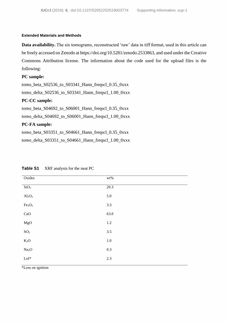
IUCrJ (2019). 6, doi:10.1107/S2052252519003774 Supporting information, sup-1
Extended Materials and Methods
Data availability. The six tomograms, reconstructed ‘raw’ data in tiff format, used in this article can
be freely accessed on Zenodo at https://doi.org/10.5281/zenodo.2533863, and used under the Creative
Commons Attribution license. The information about the code used for the upload files is the
following:
PC sample:
tomo_beta_S02536_to_S03341_Hann_freqscl_0.35_0xxx
tomo_delta_S02536_to_S03341_Hann_freqscl_1.00_0xxx
PC-CC sample:
tomo_beta_S04692_to_S06001_Hann_freqscl_0.35_0xxx
tomo_delta_S04692_to_S06001_Hann_freqscl_1.00_0xxx
PC-FA sample:
tomo_beta_S03351_to_S04661_Hann_freqscl_0.35_0xxx
tomo_delta_S03351_to_S04661_Hann_freqscl_1.00_0xxx
Table S1 XRF analysis for the neat PC
Oxides wt%
SiO2 20.3
Al2O3 5.0
Fe2O3 3.3
CaO 63.0
MgO 1.2
SO3 3.5
K2O 1.0
Na2O 0.3
LoI* 2.3
*Loss on ignition
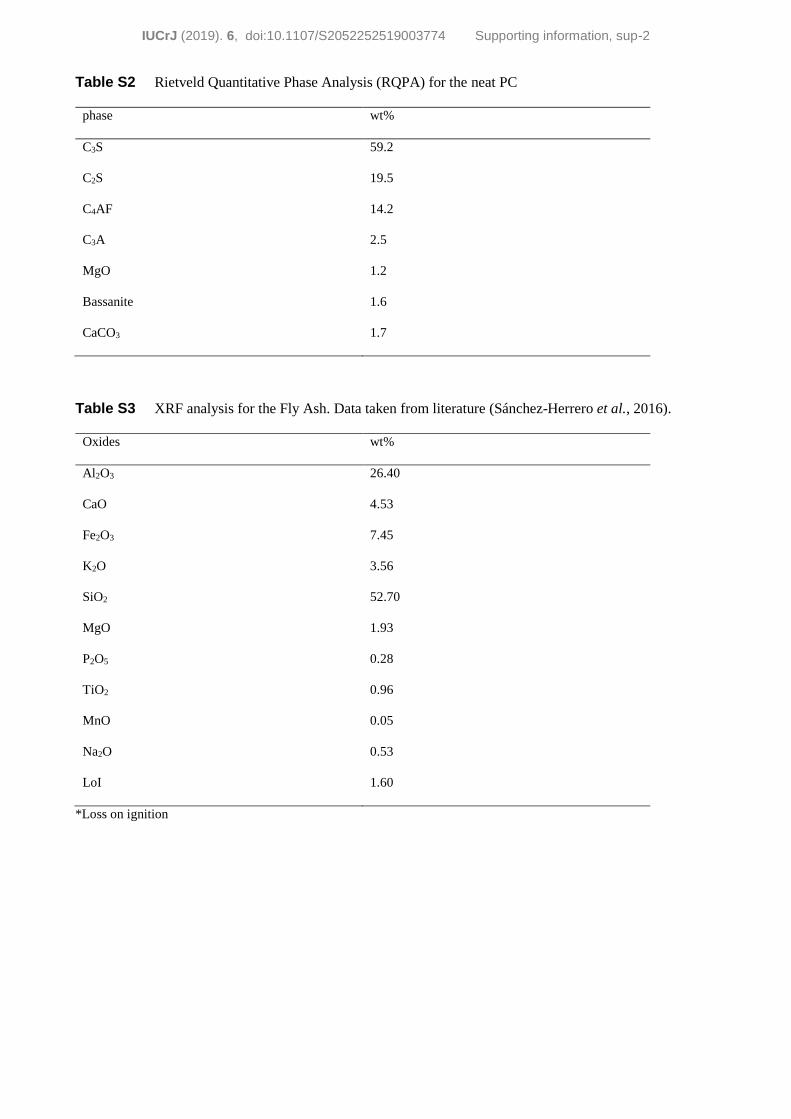
IUCrJ (2019). 6, doi:10.1107/S2052252519003774 Supporting information, sup-2
Table S2 Rietveld Quantitative Phase Analysis (RQPA) for the neat PC
phase wt%
C3S 59.2
C2S 19.5
C4AF 14.2
C3A 2.5
MgO 1.2
Bassanite 1.6
CaCO3 1.7
Table S3 XRF analysis for the Fly Ash. Data taken from literature (Sánchez-Herrero et al., 2016).
Oxides wt%
Al2O3 26.40
CaO 4.53
Fe2O3 7.45
K2O 3.56
SiO2 52.70
MgO 1.93
P2O5 0.28
TiO2 0.96
MnO 0.05
Na2O 0.53
LoI 1.60
*Loss on ignition
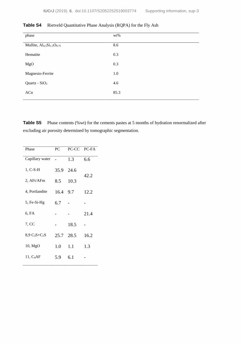
IUCrJ (2019). 6, doi:10.1107/S2052252519003774 Supporting information, sup-3
Table S4 Rietveld Quantitative Phase Analysis (RQPA) for the Fly Ash
phase wt%
Mullite, Al4.5Si1.5O9.75 8.6
Hematite 0.3
MgO 0.3
Magnesio-Ferrite 1.0
Quartz - SiO2 4.6
ACn 85.3
Table S5 Phase contents (%wt) for the cements pastes at 5 months of hydration renormalized after
excluding air porosity determined by tomographic segmentation.
Phase PC PC-CC PC-FA
Capillary water - 1.3 6.6
1, C-S-H 35.9 24.6 42.2
2, AFt/AFm 8.5 10.3
4, Portlandite 16.4 9.7 12.2
5, Fe-Si-Hg 6.7 - -
6, FA - - 21.4
7, CC - 18.5 -
8,9 C3S+C2S 25.7 28.5 16.2
10, MgO 1.0 1.1 1.3
11, C4AF 5.9 6.1 -
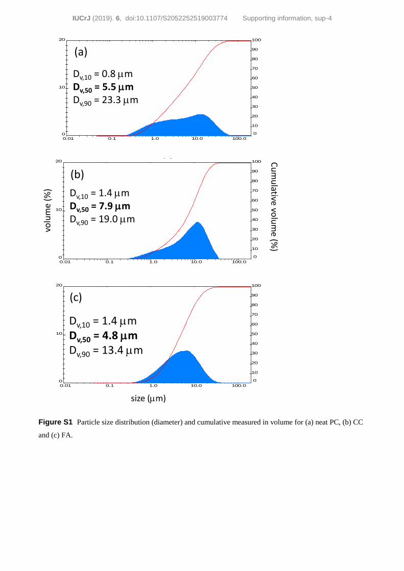
IUCrJ (2019). 6, doi:10.1107/S2052252519003774 Supporting information, sup-4
Figure S1 Particle size distribution (diameter) and cumulative measured in volume for (a) neat PC, (b) CC
and (c) FA.
Particle Diameter (µm.)
Volume (%)
0
10
20
0
10
20
30
40
50
60
70
80
90
100
0.01 0.1 1.0 10.0 100.0
Particle Diameter (µm.)
Volume (%)
0
10
20
0
10
20
30
40
50
60
70
80
90
100
0.01 0.1 1.0 10.0 100.0
Particle Diameter (µm.)
Volume (%)
0
10
20
0
10
20
30
40
50
60
70
80
90
100
0.01 0.1 1.0 10.0 100.0
Dv,10 = 0.8 mDv,50 = 5.5 mDv,90 = 23.3 m
Dv,10 = 1.4 mDv,50 = 7.9 mDv,90 = 19.0 m
Dv,10 = 1.4 mDv,50 = 4.8 mDv,90 = 13.4 m
size (m)
volu
me
(%)
Cu
mu
lativevo
lum
e(%
)
(a)
(b)
(c)
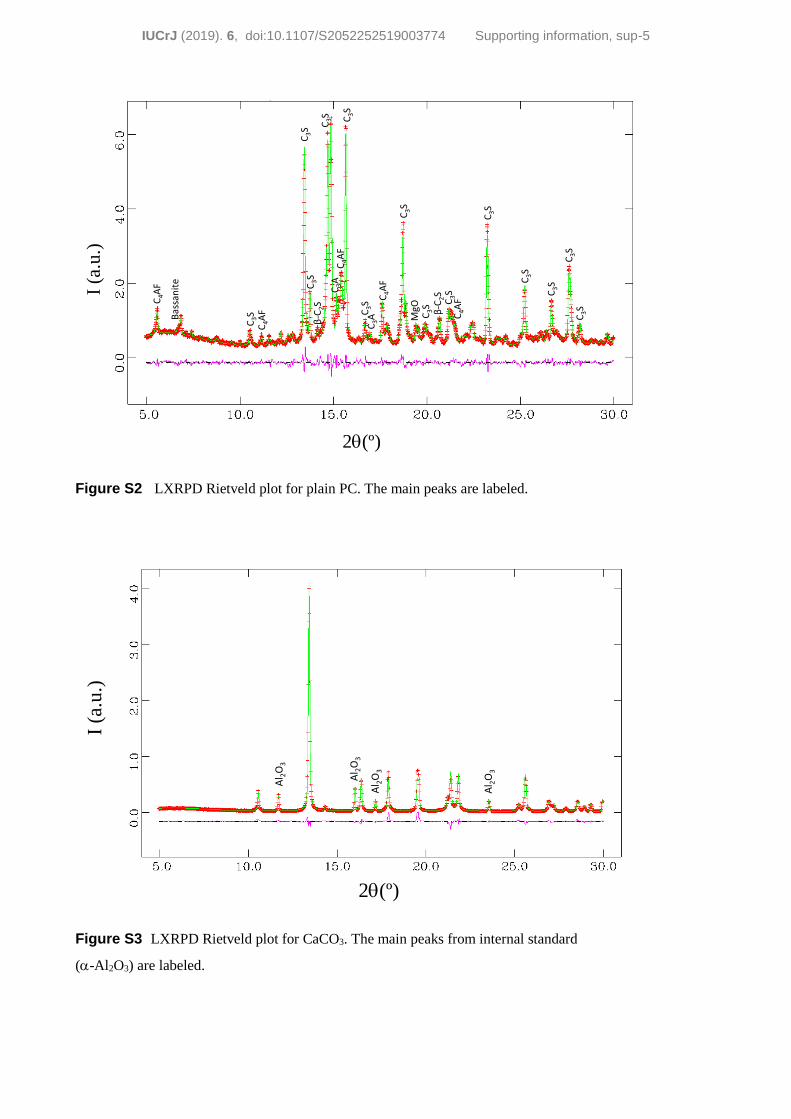
IUCrJ (2019). 6, doi:10.1107/S2052252519003774 Supporting information, sup-5
Figure S2 LXRPD Rietveld plot for plain PC. The main peaks are labeled.
Figure S3 LXRPD Rietveld plot for CaCO3. The main peaks from internal standard
(-Al2O3) are labeled.
2q(º)
I (a
.u.)
C3S
β-C
2SC
3S
C3S C
3SC
4AF
C3A
C4A
F
Bas
san
ite
C3A
C4A
F
C3S
C3S
C3S
C3S
C3S
C3S
C4A
F β-C
2S
MgO
C3S
C3S
C3S
C3SC4A
F
2q(º)
I (a
.u.)
Al 2
O3
Al 2
O3
Al 2
O3
Al 2
O3
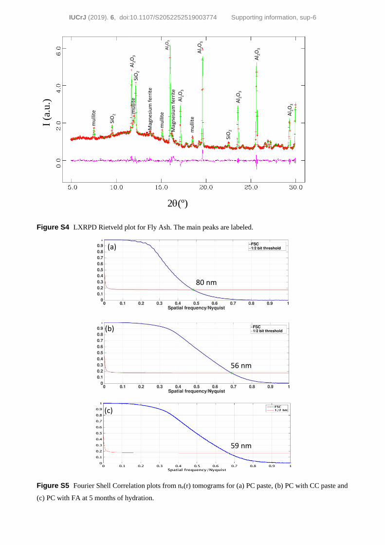
IUCrJ (2019). 6, doi:10.1107/S2052252519003774 Supporting information, sup-6
Figure S4 LXRPD Rietveld plot for Fly Ash. The main peaks are labeled.
Figure S5 Fourier Shell Correlation plots from ne(r) tomograms for (a) PC paste, (b) PC with CC paste and
(c) PC with FA at 5 months of hydration.
2q(º)
I (a
.u.)
Al 2
O3
Al 2
O3
Al 2
O3
Al 2
O3
SiO
2
SiO
2
SiO
2
mu
llite
mu
llite
mu
llite
Mag
nes
ium
fer
rite
Mag
nes
ium
fer
rite
Al 2
O3
Al 2
O3
Al 2
O3
mu
llite
80 nm
56 nm
59 nm
(a)
(b)
(c)
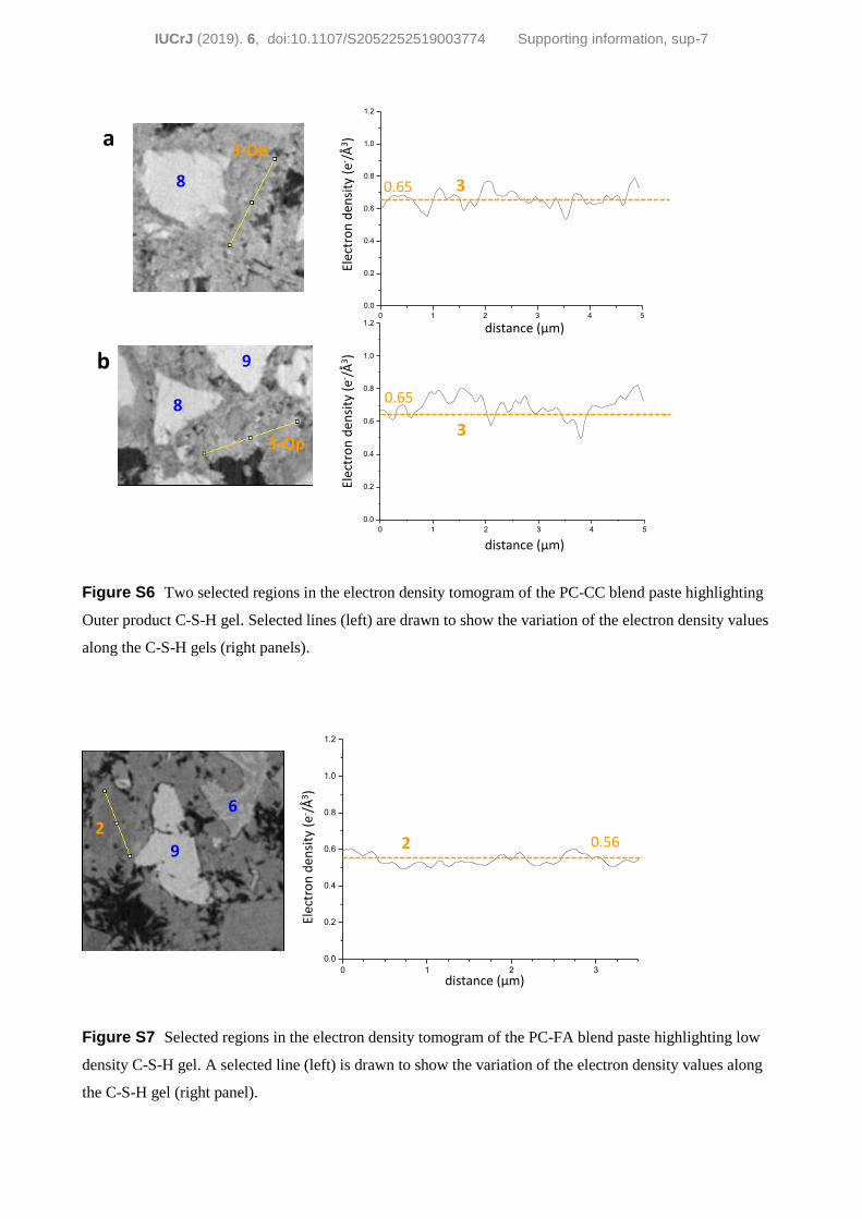
IUCrJ (2019). 6, doi:10.1107/S2052252519003774 Supporting information, sup-7
Figure S6 Two selected regions in the electron density tomogram of the PC-CC blend paste highlighting
Outer product C-S-H gel. Selected lines (left) are drawn to show the variation of the electron density values
along the C-S-H gels (right panels).
Figure S7 Selected regions in the electron density tomogram of the PC-FA blend paste highlighting low
density C-S-H gel. A selected line (left) is drawn to show the variation of the electron density values along
the C-S-H gel (right panel).
0 1 2 3 4 5
0.0
0.2
0.4
0.6
0.8
1.0
1.2
0.65 38
3-Op
0 1 2 3 4 5
0.0
0.2
0.4
0.6
0.8
1.0
1.2
0.65
3
8
3-Op
9
distance (µm)
Elec
tro
n d
ensi
ty (
e- /Å
3)
distance (µm)El
ectr
on
den
sity
(e- /
Å3)a
b
0 1 2 3
0.0
0.2
0.4
0.6
0.8
1.0
1.2
0.5629
62
distance (µm)
Elec
tro
n d
ensi
ty (
e- /
Å3)
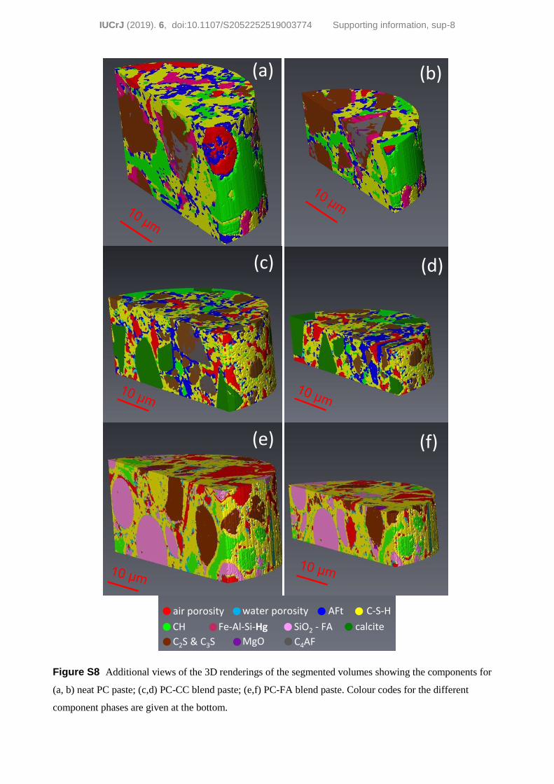
IUCrJ (2019). 6, doi:10.1107/S2052252519003774 Supporting information, sup-8
Figure S8 Additional views of the 3D renderings of the segmented volumes showing the components for
(a, b) neat PC paste; (c,d) PC-CC blend paste; (e,f) PC-FA blend paste. Colour codes for the different
component phases are given at the bottom.
(a)
(c)
(e)
(b)
(d)
(f)
air porosity water porosity AFt C-S-H
CH Fe-Al-Si-Hg SiO2 - FA calcite
C2S & C3S MgO C4AF

IUCrJ (2019). 6, doi:10.1107/S2052252519003774 Supporting information, sup-9
Figure S9 Volume of the different components as function of time in hydrating PC paste (w/s mass ratio =
0.27) modelled by GEMS
Figure S10 Volume of the different components as function of time in hydrating PC-CC paste (w/s mass
ratio = 0.27) modelled by GEMS
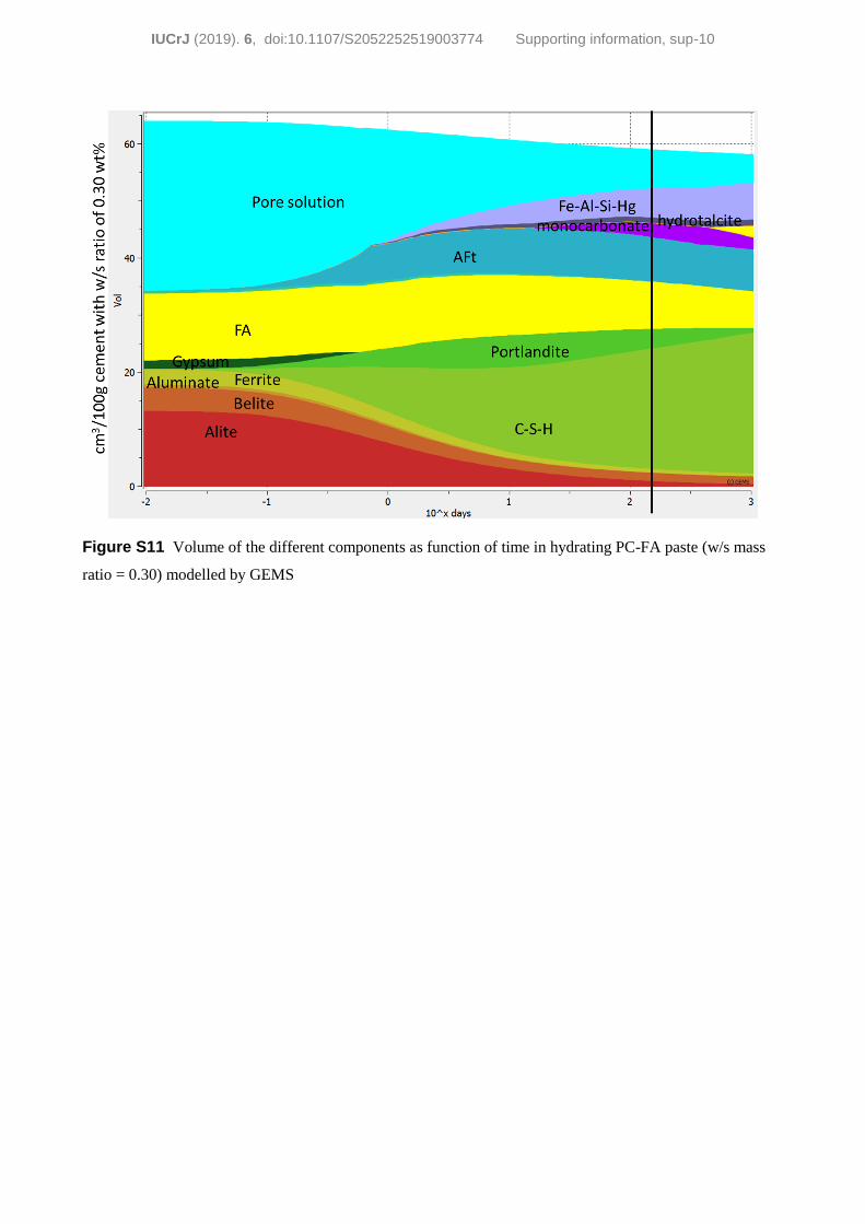
IUCrJ (2019). 6, doi:10.1107/S2052252519003774 Supporting information, sup-10
Figure S11 Volume of the different components as function of time in hydrating PC-FA paste (w/s mass
ratio = 0.30) modelled by GEMS
IUCrJ (2019). 6, doi:10.1107/S2052252519003774 Supporting information, sup-11
PXCT experiments and data processing.
The PXCT experiments took place at the cSAXS beamline at the Swiss Light Source, Paul Scherrer
Institute in Villigen, Switzerland, using the instrumentation previously reported in Holler et al. (2014,
2012), which uses laser interferometry for accurate positioning of the specimen with respect to the
beam-defining optics (Holler & Raabe, 2015). A Si (111) monochromator set the X-ray photon energy
to 6.2 keV. The illumination on the sample was defined by a coherently illuminated gold Fresnel zone
plate (Gorelick et al., 2011) of 170 μm diameter and outermost zone width of 60 nm, which for this
energy had a focal length of 51 mm focal. We estimate that the flux at the sample position was about
1.3×10⁸ photons/s. The sample was placed at 2.7 mm downstream the focus, such that the illumination
on the sample has a diameter of about 9 m. For ptychographic scans, the samples were scanned at
positions following a pattern based on Fermat spirals, as described in Huang et al. (2014). The scans
covered areas of 60×30, 65×33 and 64×30 m2 with average step sizes of about 2.5, 3 and 3 m,
resulting in an approximate number of 290, 240 and 207 points/scan for the PC, PC-CC and PC-FA
samples, respectively. Far-field diffraction patterns were recorded at each scanning position with an
acquisition time of 0.08 s using an EIGER 500k detector (Dinapoli et al., 2011) with a pixel size of
75 μm. The detector was placed at 7.305 m distance from the sample, such that ptychography
sampling conditions were satisfied (da Silva & Menzel, 2015; Edo et al., 2013). From each diffraction
pattern, a region of 500×500 pixels of the detector area was used for ptychographic reconstructions,
obtaining a pixel size of 38.95 nm in the reconstructed images. A flight tube flushed with He was
positioned between the sample and the detector to reduce the air scattering and absorption. The
different tomographic projections were acquired using a binary acquisition strategy with 8 interlaced
nests of projections as described by Kaestner et al. (2011). We acquired 800 projections within the
angular range of 0○ and 180○ for the PC paste and 1300 projections for the PC-FA and PC-CC pastes.
The dose imparted on the specimens during acquisition was estimated to range between 2.1×10⁷ Gy
for the AFt phase in the neat PC sample to 4.5×10⁷ Gy for the C3S phase in the PC-CC sample. For
this estimation the surface dose was calculated as described in (Howells et al., 2009) using the values
for the attenuation coefficient and density resulting from the Avizo image analysis and detailed in
Tables 3, 4 and 5- in the main article.
Ptychographic reconstructions were performed with a few hundred iterations of a difference map
algorithm (Thibault, 2009) followed by a few hundred iterations of a maximum likelihood
optimization used as a refinement (Thibault & Guizar-Sicairos, 2012). Before tomographic
reconstruction, the phase projections were processed to remove zero and 1st linear terms, followed by
phase unwrapping and vertical alignment (Guizar-Sicairos et al., 2011). In addition, the horizontal
alignment of the projections was performed using a tomographic consistency approach (Guizar-
Sicairos et al., 2015). The alignment corrections determined in this way were later also applied to the
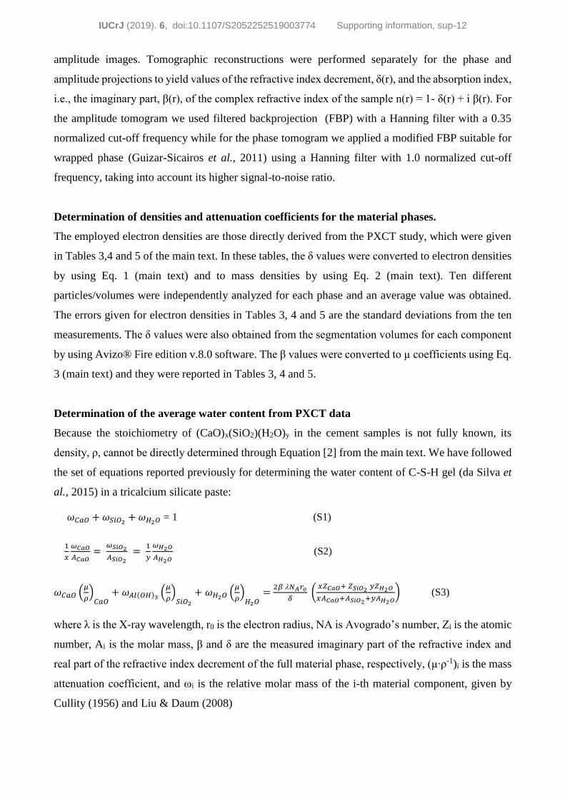
IUCrJ (2019). 6, doi:10.1107/S2052252519003774 Supporting information, sup-12
amplitude images. Tomographic reconstructions were performed separately for the phase and
amplitude projections to yield values of the refractive index decrement, δ(r), and the absorption index,
i.e., the imaginary part, β(r), of the complex refractive index of the sample n(r) = 1- δ(r) + i β(r). For
the amplitude tomogram we used filtered backprojection (FBP) with a Hanning filter with a 0.35
normalized cut-off frequency while for the phase tomogram we applied a modified FBP suitable for
wrapped phase (Guizar-Sicairos et al., 2011) using a Hanning filter with 1.0 normalized cut-off
frequency, taking into account its higher signal-to-noise ratio.
Determination of densities and attenuation coefficients for the material phases.
The employed electron densities are those directly derived from the PXCT study, which were given
in Tables 3,4 and 5 of the main text. In these tables, the δ values were converted to electron densities
by using Eq. 1 (main text) and to mass densities by using Eq. 2 (main text). Ten different
particles/volumes were independently analyzed for each phase and an average value was obtained.
The errors given for electron densities in Tables 3, 4 and 5 are the standard deviations from the ten
measurements. The δ values were also obtained from the segmentation volumes for each component
by using Avizo® Fire edition v.8.0 software. The β values were converted to µ coefficients using Eq.
3 (main text) and they were reported in Tables 3, 4 and 5.
Determination of the average water content from PXCT data
Because the stoichiometry of (CaO)x(SiO2)(H2O)y in the cement samples is not fully known, its
density, ρ, cannot be directly determined through Equation [2] from the main text. We have followed
the set of equations reported previously for determining the water content of C-S-H gel (da Silva et
al., 2015) in a tricalcium silicate paste:
𝜔𝐶𝑎𝑂 + 𝜔𝑆𝑖𝑂2+ 𝜔𝐻2𝑂 = 1 (S1)
1
𝑥
𝜔𝐶𝑎𝑂
𝐴𝐶𝑎𝑂=
𝜔𝑆𝑖𝑂2
𝐴𝑆𝑖𝑂2
= 1
𝑦
𝜔𝐻2𝑂
𝐴𝐻2𝑂 (S2)
𝜔𝐶𝑎𝑂 (𝜇
𝜌)
𝐶𝑎𝑂+ 𝜔𝐴𝑙(𝑂𝐻)3
(𝜇
𝜌)
𝑆𝑖𝑂2
+ 𝜔𝐻2𝑂 (𝜇
𝜌)
𝐻2𝑂=
2𝛽𝑁𝐴𝑟𝑜
𝛿 (
𝑥𝑍𝐶𝑎𝑂+ 𝑍𝑆𝑖𝑂2 𝑦𝑍𝐻2𝑂
𝑥𝐴𝐶𝑎𝑂+𝐴𝑆𝑖𝑂2+𝑦𝐴𝐻2𝑂) (S3)
where λ is the X-ray wavelength, r0 is the electron radius, NA is Avogrado’s number, Zi is the atomic
number, Ai is the molar mass, β and δ are the measured imaginary part of the refractive index and
real part of the refractive index decrement of the full material phase, respectively, (µ∙ρ-1)i is the mass
attenuation coefficient, and ωi is the relative molar mass of the i-th material component, given by
Cullity (1956) and Liu & Daum (2008)
IUCrJ (2019). 6, doi:10.1107/S2052252519003774 Supporting information, sup-13
j
jj
iii
Aa
Aa , (S4)
where i denotes each component, namely CaO, SiO2 and H2O, and j each atom in the component. The
quantity to be determined is then aH2O, which is denoted as y in Eqs. S2 and S3. For aCaO, the 1.8
value obtained from bibliography was fixed, denoted as x in Eqs. S2 and S3 and aSiO2 is 1.
Finally, the same µ∙ρ-1values reported by da Silva et al. were used for this study, see S.I. in da Silva
et al. (2015).
References
Cullity, B. D. (1956). J. Chem. Educ. 34, A178.
Dinapoli, R., Bergamaschi, A., Henrich, B., Horisberger, R., Johnson, I., Mozzanica, A., Schmid,
E., Schmitt, B., Schreiber, A., Shi, X. & Theidel, G. (2011). Nucl. Instruments Methods Phys.
Res. Sect. A Accel. Spectrometers, Detect. Assoc. Equip. 650, 79–83.
Edo, T. B., Batey, D. J., Maiden, A. M., Rau, C., Wagner, U., Pešić, Z. D., Waigh, T. A. &
Rodenburg, J. M. (2013). Phys. Rev. A. 87, 053850.
Gorelick, S., Vila-Comamala, J., Guzenko, V. A., Barrett, R., Salomé, M. & David, C. (2011). J.
Synchrotron Radiat. 18, 442–446.
Guizar-Sicairos, M., Boon, J. J., Mader, K., Diaz, A., Menzel, A. & Bunk, O. (2015). Optica. 2,
259.
Guizar-Sicairos, M., Diaz, A., Holler, M., Lucas, M. S., Menzel, A., Wepf, R. A. & Bunk, O.
(2011). Opt. Express. 19, 21345.
Holler, M., Diaz, A., Guizar-Sicairos, M., Karvinen, P., Färm, E., Härkönen, E., Ritala, M., Menzel,
A., Raabe, J. & Bunk, O. (2014). Sci. Rep. 4, 3857.
Holler, M. & Raabe, J. (2015). 54, 054101.
Holler, M., Raabe, J., Diaz, A., Quitmann, C., Menzel, A. & Bunk, O. (2012). 83, 073703.
Howells, M. R., Beetz, T., Chapman, H. N., Cui, C., Holton, J. M., Kirz, J., Lima, E., Marchesini,
S., Miao, H., Sayre, D., Shapiro, D. A., Spence, J. C. H. & Starodub, D. (2009). J. Electron
Spectros. Relat. Phenomena. 170, 4–12.
Huang, X., Yan, H., Harder, R., Hwu, Y., Robinson, I. K. & Chu, Y. S. (2014). Opt. Express. 22,
12634.
Kaestner, A., Munch, B., Trtik, P. & Butler, L. (2011). Opt. Eng. 50, 123201.
Liu, Y. & Daum, P. H. (2008). J. Aerosol Sci. 39, 974–986.
Sánchez-Herrero, M. J., Fernández-Jiménez, A. & Palomo, Á. (2016). J. Am. Ceram. Soc. 99, 604–
611.
da Silva, J. C. & Menzel, A. (2015). Opt. Express. 23, 33812.
da Silva, J. C., Trtik, P., Diaz, A., Holler, M., Guizar-Sicairos, M., Raabe, J., Bunk, O. & Menzel,
A. (2015). Langmuir. 31, 3779–3783.
Related Documents

![Guided Variational Autoencoder for Disentanglement Learning...VAE. Recent efforts in fairness disentanglement learning [9, 47] also bear some similarity, but there is still a large](https://static.cupdf.com/doc/110x72/610df3875956a95be71207bc/guided-variational-autoencoder-for-disentanglement-learning-vae-recent-efforts.jpg)