Discrete Transform

Discrete Transform
Dec 31, 2015
Discrete Transform. Introduction. A transform maps image data into a different mathematical space via a transformation equation. One example of transform that we had encountered before is the transform from one color space to another color space. RGB to SCT (spherical coordinate transform). - PowerPoint PPT Presentation
Welcome message from author
This document is posted to help you gain knowledge. Please leave a comment to let me know what you think about it! Share it to your friends and learn new things together.
Transcript

Discrete Transform
Introduction
A transform maps image data into a different mathematical space via a transformation equation.
One example of transform that we had encountered before is the transform from one color space to another color space.– RGB to SCT (spherical coordinate transform).– RGB to HSL (hue/saturation/lightness).

Introduction
However, the transform from one color space to another color space has a one-to-one correspondence between a pixel in the input and the output.
Here, we are mapping the image data from the spatial domain to the frequency domain (spectral domain).

Introduction
All the pixels in the input (spatial domain) contribute to each value in the output (frequency domain). (see fig. 5.1.1).
Discrete transforms are performed based on specific functions, which are called the basis functions.
– These functions are typically sinusoidal or rectangular.
The discrete version of 1-D basis function are called basis vectors. (see fig. 5.1.2).
The discrete version of 2-D basis function are called basis images (or basis matrices). (see fig. 5.1.1(c)).

Figure 5.1-1 Discrete Transforms


Introduction
The process of transforming the image data into another domain involves projecting the image onto the basis images
The mathematical term for this projection process is called an inner product.– This is identical to what we have done with Frei-
Chen masks. Assuming an NxN image, the general form of
the transformation equation is as follows:
See fig: 5.1.5

Introduction
1
0
1
0
),;,(),(),(N
r
N
c
vucrBcrIvuT
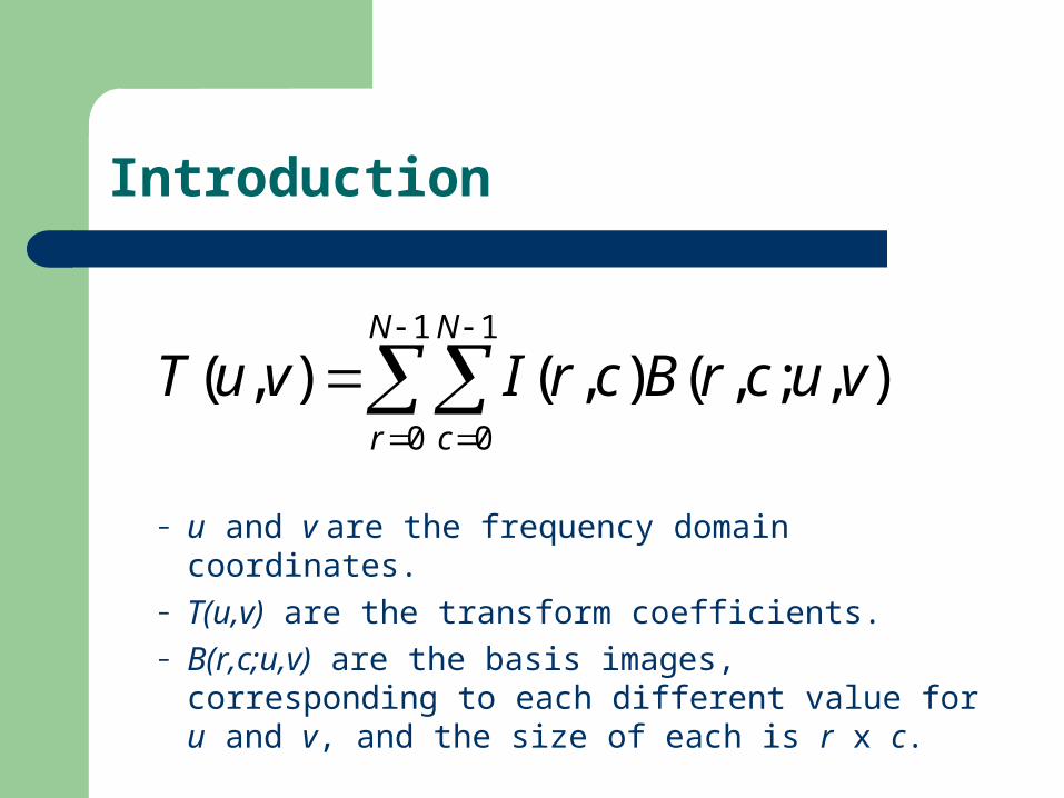
– u and v are the frequency domain coordinates.– T(u,v) are the transform coefficients.– B(r,c;u,v) are the basis images, corresponding to
each different value for u and v, and the size of each is r x c.

Introduction
The transform coefficients T(u,v) are the projection of I(r,c) onto each B(u,v).
These coefficients tell us how similar the image is to the basis image.– The more alike they are, the bigger the coefficients.
The transformation process composed the image into a weighted sum of basis images where T(u,v) are the weights.
See eg: 5.1.1

Introduction
To obtain the image from the transform coefficients, we apply the inverse transform equation:
1
0
1
0
1 ),;,(),(),(N
u
N
v
vucrBvuTcrI
See eg: 5.1.2
Introduction
Here, the B-1(r,c;u,v) represents the inverse basis images.
In many cases, the inverse basis images are the same as the forward ones, but possibly weighted by a constant.
Here, we will learn 3 types of transforms:– Walsh-Hadamard Transform, Fourier
Transform and Cosine Transform.
Walsh-Hadamard Transform
For Walsh-Hadamard, the basis functions are based on square or rectangular waves with peaks of +1 and -1.
One main advantage of rectangular basis functions is that the computations are very simple.– When we project the image onto the basis
functions, all we need to do is to multiply each pixel with +1 or -1.

Walsh-Hadamard Transform
Depending on the size of the image to be transformed, we must use basis images with the right size.– To convert an NxN image, we need to use a set
of NxN basis images.
For example, to transform a 2x2 image, then we need to use the set of 2x2 basis images as shown in the next slide.

Walsh-Hadamard Transform
11
11
11
11
11
11
11
11 The set of 2x2 Walsh-Hadamard basis images

Walsh-Hadamard Transform
Once we have the basis images, we can perform the transform operation to convert an image from the spatial domain to the frequency domain.– Project the image onto each of the basis images.– The result should be a matrix that has the same
size as the image.– This is the frequency domain of that image.

Walsh-Hadamard Transform
The equation for the whole transform operation is given below:
In this case, N refers to the dimension of the image.
1
0
)]()()()([1
0
1
0
)1(),(1
),(
n
iiiii vpcbuprbN
r
N
c
crIN
vuWH

Walsh-Hadamard Transform
To reconstruct the original image from the transform coefficients, we need to perform an inverse transform operation.
The equation is as follows:
1
0
)]()()()([1
0
1
0
)1(),(1
),(
n
iiiii vpcbuprbN
u
N
v
vuWHN
crI

Walsh-Hadamard Transform
From the equation, it can be seen that the inverse basis images is just the same as the forward basis images.
It means that the original image can be obtained by taking the transform coefficients and run it through the same operation as the one for forward transform.
Walsh-Hadamard Transform
The difference between the different types of transform is the basis images used.
Each type of transform has its own equation to be used to generate the basis images.
To make things easier, we will learn how to generate the basis vectors first, and using the basis vectors, we will generate the basis images.

Walsh-Hadamard Transform
Assuming an N-points basis vector, the equation to generate a 1-D Walsh-Hadamard basis vector is as follows:
1
0
)()(
)1(1
)(
n
iii vpcb
vN
cWH

Walsh-Hadamard Transform
– v is the index in the frequency domain.– c is the index in the spatial domain.– N is the number of points in the basis vector.– n = log2N, which is the number of bits in the
number N.– bi(c) is found by considering c as a binary number
and finding the ith bit. It means the ith bit in c.

Walsh-Hadamard Transform
– pi(v) is found as follows:
)()()(
.
.
)()()(
)()()(
)()(
011
322
211
10
vbvbvp
vbvbvp
vbvbvp
vbvp
n
nn
nn
n

Walsh-Hadamard Transform
Some examples on finding the variables:– If N = 8, then n = 3, because log28 = 3.
If c = 410 = 1002, then
b2(c) = 1, b1(c) = 0 and b0(c) = 0.
– If N = 16, then n = 4, because log216 = 4.
If c = 210 = 00102, then
b3(c) = 0, b2(c) = 0, b1(c) = 1 and b0(c) = 0.

Walsh-Hadamard Transform
Example: Building the 4-points Walsh-Hadamard basis vector set.– Start by finding the basis vector for v = 0.– The result is [1 1 1 1].
1001013(11)
1001002(10)
1000011(01)
1000000(00)
WHv(c)pi(v)bi(c)pi(v)bi(c)c
10
iv=0(002)
1
0
)()(n
iii vpcb

Walsh-Hadamard Transform
– Next, find the basis vector for v = 1.– The result is [1 1 -1 -1].
-1111013(11)
-1111002(10)
1010011(01)
1010000(00)
WHv(c)pi(v)bi(c)pi(v)bi(c)c
10
iv=1(012)
1
0
)()(n
iii vpcb

Walsh-Hadamard Transform
– Then, find the basis vector for v = 2.– The result should be [1 -1 -1 1].
1211113(11)
-1111102(10)
-1110111(01)
1010100(00)
WHv(c)pi(v)bi(c)pi(v)bi(c)c
10
iv=2(102)
1
0
)()(n
iii vpcb

Walsh-Hadamard Transform
– Finally, find the basis vector for v = 3.– The result it [1 -1 1 -1].
-1321113(11)
1221102(10)
-1120111(01)
1020100(00)
WHv(c)pi(v)bi(c)pi(v)bi(c)c
10
iv=3(112)
1
0
)()(n
iii vpcb

Walsh-Hadamard Transform
Using the the 1-D basis vectors, we can generate the 2-D Walsh-Hadamard basis images.
Example: Generating the 4x4 basis image for u = 3 and v = 2.– Look at the basis vector for index 3 and 2.– For index 3: [1 -1 1 -1]– For index 2: [1 -1 -1 1]

Walsh-Hadamard Transform
+1 -1 -1 +1
-1 +1 +1 -1
+1 -1 -1 +1
-1 +1 +1 -1
+1
-1
+1
-1
+1 -1 -1 +1
1-D basis vector for v = 2
1-D basis vector for u = 3
Fill in the matrix by multiplying the corresponding row and columns.

Walsh-Hadamard Transform
Remember that we need to scale the resulting matrix by 1 / √N.– In this case, N = 16, and therefore √N = 4.
1111
1111
1111
1111
4
132WH

Walsh-Hadamard Transform
By finding the basis images for every combination of u and v, we can get a set of Walsh-Hadamard basis images.
The set of 4x4 Walsh-Hadamard basis images are shown in the next slide.– White color corresponds to +1.– Black color corresponds to -1.

Walsh-Hadamard Transform

Fourier Transform
The Fourier transform is the most well known, and the most widely used, transform.
Fourier transform is used in many applications:– Vibration analysis in mechanical engineering.– Circuit analysis in electrical engineering.– Computer imaging.

Fourier Transform
Fourier transform decomposes an image into a weighted sum of 2-D sinusoidal term.
The general formula to generate the N-points 1-D Fourier basis vector set is as follows:
N
vcj
N
vce
NcF N
vcj
v
2sin
2cos
1)(
2

Fourier Transform
The equation for the Fourier basis vector can be written in two different formats because of Euler’s identity:– ejx = cos x + j sin x
Notice that the basis vector consists of complex numbers.

Fourier Transform
Example: Building the 4-points Fourier basis vector set.– Start by finding the basis vector for v = 0.– The result is [1 1 1 1].
N
vc2)
2cos(
N
vc)
2sin(
N
vcj
)(cFv
1-j0103
1-j0102
1-j0101
1-j0100
c
Fourier Transform
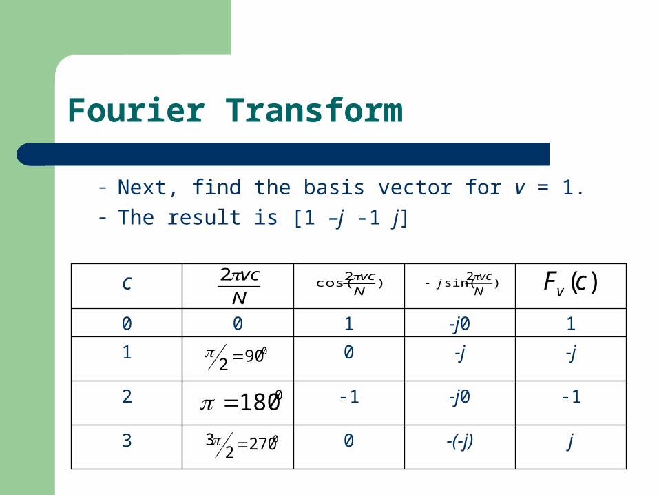
– Next, find the basis vector for v = 1.– The result is [1 –j -1 j]
N
vc2)
2cos(
N
vc)
2sin(
N
vcj
)(cFv
0902
018002702
3 j-(-j)03
-1-j0-12
-j-j01
1-j0100
c

Fourier Transform
– Then, find the basis vector for v = 2.– The result is [1 -1 1 -1]
N
vc2)
2cos(
N
vc)
2sin(
N
vcj
)(cFv
0180
00 03602 00 1805403 -1-j0-13
1-j012
-1-j0-11
1-j0100
c
Fourier Transform
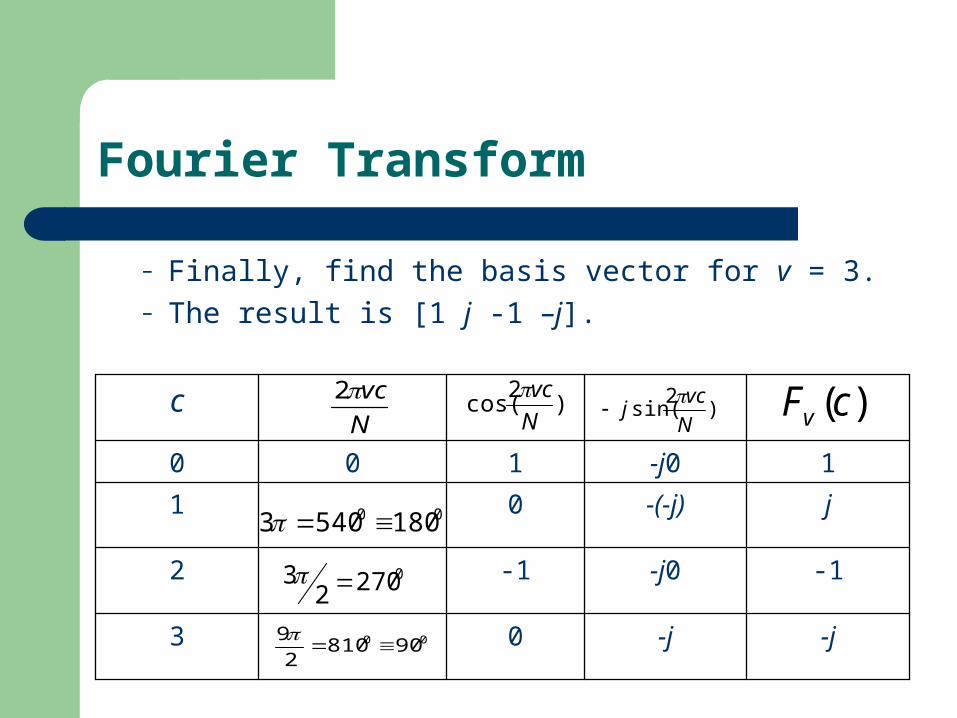
– Finally, find the basis vector for v = 3.– The result is [1 j -1 –j].
N
vc2)
2cos(
N
vc)
2sin(
N
vcj
)(cFv
027023
00 1805403
00 908102
9
-j-j03
-1-j0-12
j-(-j)01
1-j0100
c

Fourier Transform
As in Walsh-Hadamard, the 2-D Fourier basis images can be generated from the 1-D Fourier basis vector.
Example: Generating the 4x4 basis image for u = 3 and v = 2.– Look at the basis vector for index 3 and 2.– For index 3: [1 j -1 -j]– For index 2: [1 -1 1 -1]

Fourier Transform
+1 -1 +1 -1
+j -j +j -j
-1 +1 -1 +1
-j +j -j +j
+1
+j
-1
-j
+1 -1 +1 -1
1-D basis vector for v = 2
1-D basis vector for u = 3
Fill in the matrix by multiplying the corresponding row and columns.

Fourier Transform
Remember that we need to scale the resulting matrix by 1 / √N.– In this case, N = 16, and therefore √N = 4.
jjjj
jjjjF
1111
1111
4
132

Fourier Transform
Once all the required basis images have been obtained, then we can perform the transform operation.
The equation for Fourier transform operation is as follows:
N
vcurjN
r
N
c
ecrIN
vuF)(
21
0
1
0
),(1
),(

Fourier Transform
Due to Euler’s identity, the previous equation can also be written as follows:
Since the Fourier basis images are complex, the Fourier transform coefficients F(u,v) are also complex.– Real part: cosine terms.– Imaginary part: sine terms
))](2
sin())(2
cos()[,(1
),(1
0
1
0
vcurN
jvcurN
crIN
vuFN
r
N
c

Fourier Transform
After we perform the transform, we can get back the original image by applying the inverse Fourier transform.
The equation for inverse Fourier transform is as follows:
N
vcurjN
u
N
v
evuFN
crI)(
21
0
1
0
),(1
),(

Fourier Transform
Notice that in the inverse Fourier transform, the basis function used is the complex conjugate of the one used in forward transform.– The exponent sign is changed from -1 to +1.– In the sine-cosine format, this will change the sign
of the imaginary component.– Therefore, it changes the phase of the basis
functions

Cosine Transform
Similar to Fourier transform, cosine transform also uses sinusoidal basis functions.
The difference is that the cosine transform basis functions are not complex.– They use only cosine functions and not sine
functions.
The general formula to generate the N-points 1-D cosine basis vector set is as follows:

Cosine Transform
1,...2,12
01
)(
2
)12(cos)()(
NvforN
vforNv
N
vnvnCv

Cosine Transform
The equation is almost the same as the previous two transforms except that the scaling factor is not the same for all the basis vectors.
Once the 1-D basis vectors have been obtained, the 2-D basis images can be generated in the same manner as in the previous transforms.

Cosine Transform
The basis images generated can be used in both the forward transform and also the inverse transform.
Cosine transform is often used in image and video compression algorithms such as JPEG, MPEG, H.263, etc.
The diagram in the next slide shows the cosine transform basis image values represented as gray-level values.

Cosine Transform
B(r,c) Gray Level
-0.43 0
-0.33 30
-0.25 54
-0.18 75
-0.14 86
-0.07 106
0.07 149
0.14 170
0.18 181
0.25 202
0.33 225
0.43 255

Separable Properties
All the three transform that we have discussed earlier have separable properties.
If a 2-D transform is separable, then the result can be found by successive application of two 1-D transforms.
This means that we can perform 2-D transform using only the 1-D basis vectors, without having to generate the 2-D basis images.

Separable Properties
Let us perform a 2-D Walsh-Hadamard transform on a 2x2 image using only the 1-D Walsh-Hadamard basis vectors.
The 2-points Walsh-Hadamard basis vectors are as follows:– WH0 = [+1 +1]
– WH1 = [+1 -1]

Separable Properties
Assume that we have this 2x2 image:
First we perform the 1-D Walsh-Hadamard transform on each row (or column).– Perform vector inner product between the basis
vector and the image row.
5040
3020),( crI

Separable Properties
The result is as follows:
Next, we perform the 1-D Walsh-Hadamard transform on each column (or row) of the resulting transform image.– Perform the inner product between basis vector
and the resulting image column.
1090
1050
)1(50)1(40)1(50)1(40
)1(30)1(20)1(30)1(20'T

Separable Properties
The result is as follows:
Remember to scale the result by ½.
040
20140
)1)(10()1)(10()1(90)1(50
)1)(10()1)(10()1(90)1(50''T
020
1070
040
20140
2
1T

Separable Properties
You can verify that this result is the same as in using the 2-D Walsh-Hadamard basis images.
The advantage of this method is that it requires less computation.– Using 2-D method: N4 multiplications and (N4-N2)
additions.– Using 1-D method: 2N3 multiplications and 2(N3-
N2) additions.

Interpretation of Transformed Image
The transformed image represents the intensity of various spatial frequency.
For Walsh-Hadamard and Cosine Transform, the top left corner of the transformed image is associated with zero frequency.– Zero frequency often referred to as DC (direct
current).– The non-zero frequencies are referred to as AC
(alternate current).

Interpretation of Transformed Image
The transformed coefficients represent higher and higher frequency as it goes from top left to bottom right of the transformed image.
By knowing what the transformed image represents, we can perform filtering operations in the frequency domain to modify the image according to our needs.

Filtering
Filtering in the frequency domain involves eliminating or reducing some parts of the frequency components of an image.
Here, we will discuss a number of different types of filters:– Lowpass filters– Highpass filters– Bandpass/bandreject filters
Filtering – Lowpass Filter
Lowpass filters pass low frequencies and attenuate or eliminate the high frequency information.– This operation tends to blur the image.– Often used for image compression or for hiding
effects caused by noise.
Lowpass filtering is performed by multiplying the spectrum by a filter.

Filtering – Lowpass Filter
To obtained the filtered image, we need to perform the inverse transform.
An ideal lowpass filter contains only 1 and 0. The frequency at which we start to eliminate
information is called the cutoff frequency, f0. The frequencies that get filtered out are in
the stopband, while the frequencies that are not filtered out are in the passband.

Filtering – Lowpass Filter

Filtering – Lowpass Filter

Filtering – Lowpass Filter
The filtering process can be represented by the following equation:
– Ifil(r,c) is the filtered image
– H(u,v) is the filter function– T(u,v) is the transform coefficients– T-1 represents the inverse transform operation
)],(),([),( 1 vuHvuTTcrI fil

Filtering – Lowpass Filter
The multiplication T(u,v)H(u,v) is performed with a point-to-point method.– T(0,0) is multiplied by H(0,0), T(0,1) is multiplied
by H(0,1) and so on.
For ideal filters, H(u,v) will contain only 1’s and 0’s.
For non-ideal filters, other values are also possible.

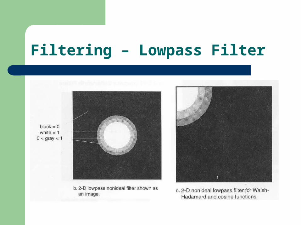
Filtering – Lowpass Filter
Ideal filters can leaves undesirable artifacts in images.– This artifact appears as ripples.

Filtering – Lowpass Filter
This problem can be avoided by using a “non-ideal” filter that does not have perfect transition.
There is one type of non-ideal filter called the Butterworth filter that allows user to specify the order of the filter.– The higher the order, the steeper the transition
slope, the closer it is to ideal filter.

Filtering – Lowpass Filter
Filtering – Lowpass Filter
Filtering – Lowpass Filter
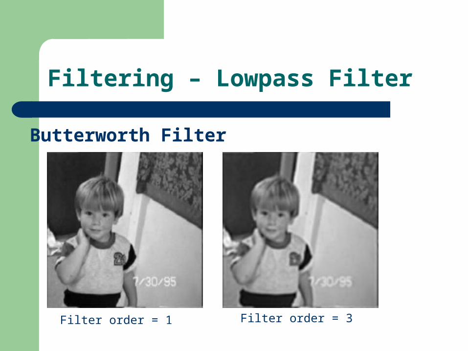
Butterworth Filter
Filter order = 1 Filter order = 3

FilteringFiltering – Lowpass Filter
Butterworth Filter
Filter order = 6 Filter order = 8
Filtering – Lowpass Filter
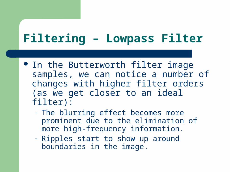
In the Butterworth filter image samples, we can notice a number of changes with higher filter orders (as we get closer to an ideal filter):– The blurring effect becomes more prominent due
to the elimination of more high-frequency information.
– Ripples start to show up around boundaries in the image.

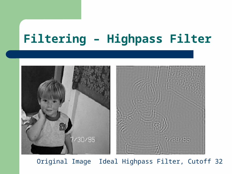
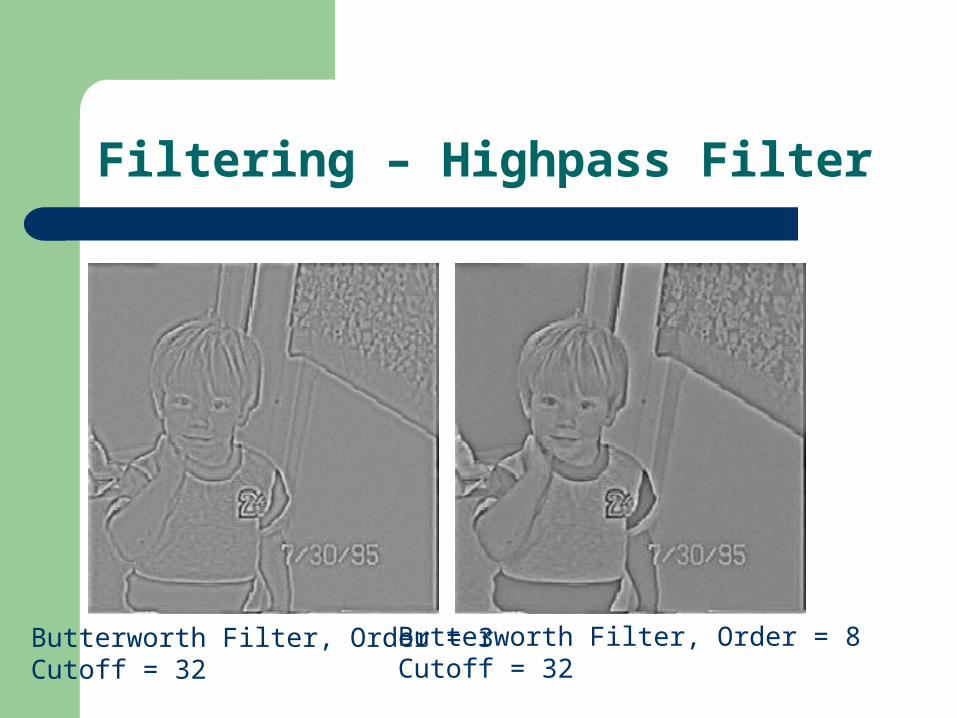
Filtering – Highpass Filter
Highpass filters pass high frequencies and attenuate or eliminate the low frequency information.– High-frequency information corresponds to places
where gray-levels are changing rapidly – Can be used to enhance edges.– Overall image contrast will be lost due to
elimination of low frequency components.

Filtering – Highpass Filter

Filtering – Highpass Filter

Filtering – Highpass Filter
Filtering – Highpass Filter
Original Image Ideal Highpass Filter, Cutoff 32
Filtering – Highpass Filter
Butterworth Filter, Order = 3Cutoff = 32
Butterworth Filter, Order = 8Cutoff = 32

Filtering – Highpass Filter
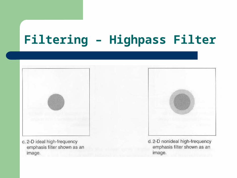
A variation of the highpass filter called the high-frequency emphasis filter can retain some of the low frequency by adding an offset value.– This will retain some of the overall contrast.
Filtering – Highpass Filter

Filtering – Highpass Filter

Filtering – Highpass Filter
Highpass Emphasis FilterOffset = 0.5, Order = 2Cutoff = 32
Highpass Emphasis FilterOffset = 1.5, Order = 2Cutoff = 32

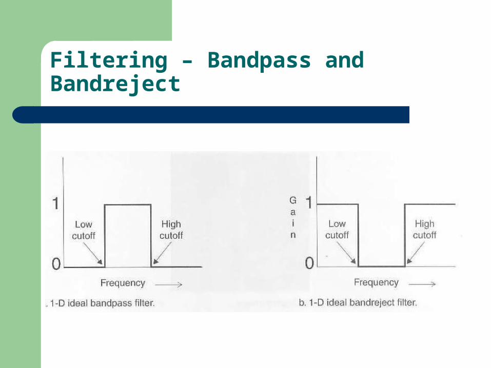
Filtering – Bandpass and Bandreject
The bandpass and bandreject filters are specified by two cutoff frequencies, a low cutoff and a high cutoff.
A special form of these filters is called a notch filter because it only passes out specific frequencies.
These filters are typically used in image restoration, enhancement and compression.
Filtering – Bandpass and Bandreject

Filtering – Bandpass and Bandreject

Filtering – Bandpass and Bandreject

Filtering – Bandpass and Bandreject
Related Documents