Uniform Discrete Curvelet Transform

3618 IEEE TRANSACTIONS ON SIGNAL PROCESSING, VOL. 58, NO. 7, JULY 2010

Uniform Discrete Curvelet TransformTruong T. Nguyen and Hervé Chauris

Abstract—An implementation of the discrete curvelet transformis proposed in this work. The transform is based on and has thesame order of complexity as the Fast Fourier Transform (FFT).The discrete curvelet functions are defined by a parameterizedfamily of smooth windowed functions that satisfies two conditions:i) �� periodic; ii) their squares form a partition of unity. Thetransform is named the uniform discrete curvelet transform(UDCT) because the centers of the curvelet functions at eachresolution are positioned on a uniform lattice. The forward andinverse transform form a tight and self-dual frame, in the sensethat they are the exact transpose of each other. Generalizationto � dimensional version of the UDCT is also presented. Thenovel discrete transform has several advantages over existingtransforms, such as lower redundancy ratio, hierarchical datastructure and ease of implementation.

Index Terms—Contourlet, curvelet, directional decomposition,directional filter bank, multidimensional filter bank, multiresolu-tion representation, wavelet.

I. INTRODUCTION

D URING the last two decades, there have been a lot of re-search activities on new mathematical and computational

tools for multiresolution data representation. The wavelet trans-form, arising from a particular question in geophysics, decom-poses a function on the real line to a sum of local wave-like func-tions at multiple scales. It is shown that the continuous waveletfunctions and their discrete counterpart implemented by reg-ular filter banks are optimal representations of one dimensionalpiece-wise smooth signals [1]. However, the direct extensionof a wavelet to two dimensions by the tensor product of twoone-dimensional wavelets is no longer optimal for representinga signal that has features along smooth curves [2]. There havebeen many 2-D transforms with directional basis that can betterrepresent this type of signal. Without being exhaustive, we listseveral examples of directional, discrete and nonadaptive trans-forms such as the steerable pyramid [3], the complex wavelet[4], [5], discrete curvelet [6], shearlet transforms [7], and con-tourlet transform [8].

Recently, Candès and Donoho constructed the curvelet trans-form [9], and proved that it is an essentially optimal represen-

Manuscript received May 27, 2009; accepted February 21, 2010. Date of pub-lication April 05, 2010; date of current version June 16, 2010. The associate ed-itor coordinating the review of this manuscript and approving it for publicationwas Dr. Soontorn Oraintara. This work was supported in part by Shell E&P.

T. T. Nguyen is with the R&D Department, Fugro Seismic Imaging, Swanley,U.K. (e-mail: [email protected]).

H. Chauris is with the Centre de Géosciences, Mines ParisTech, UMRSisyphe 7619, Fontainebleau, 77300 France (e-mail: [email protected]).

Color versions of one or more of the figures in this paper are available onlineat http://ieeexplore.ieee.org.

Digital Object Identifier 10.1109/TSP.2010.2047666

tation of two-variable functions, which are smooth except atdiscontinuities along (twice differentiable) curve. The non-linear approximation of a function , , reconstructed by

largest curvelet coefficients has an asymptotic decay rate of

. This decay rate of the ap-proximation error is a significant theoretical improvement com-pared to those by wavelets or Fourier coefficients, which are

and , respectively [1]. The 2-D curvelettransform decomposes a signal into a sum of basis functionsthat represent local waves with strong directionality. The effec-tive support of these curvelet functions are highly anisotropic atfine scale, following a parabolic scaling rule: length width.

It has been proved that curvelet representation for wave prop-agation is optimally sparse [10]. It is argued that the represen-tation of seismic data by the curvelet transform is also opti-mally sparse and a series of applications can be found in the areaof seismic imaging [11]–[13]. The curvelet transform has alsofound applications in other areas of image processing [14]–[16].

In the last few years, several discrete curvelet and curvelet-like transforms have been proposed. They can be divided intodiscrete transforms based on the fast Fourier transform (FFT)[6], [17], or based on filter bank (FB) implementations [8], [18],[19].

The major contribution of this paper is a new discrete curvelettransform that uses the ideas of both FFT-based discrete curvelettransform and filter-bank based contourlet transform. The moti-vation of the new transform is from the difficulties we encoun-tered while trying to use curvelet transform in real world appli-cations. The new uniform discrete curvelet transform (UDCT)is implemented by the FFT algorithm, but it is designed as amultiresolution filter bank. By this way, we are able to takeadvantage of the two methods. For example, the new curveletbasis functions have excellent frequency responses, which is notpossible with the contourlet transform. The UDCT has signifi-cantly lower redundancy compared to other FFT-based discretecurvelet transforms [6], [17], especially in high-dimension ver-sion of the transform. This makes the UDCT very practical inindustrial applications.

Paper Outline: In the next section the notations used in thispaper are introduced. Since the UDCT is interpreted as a mul-tiresolution FB, this section also includes a short review of someformulae for multidimensional multirate systems. The curveletand contourlet transforms are reviewed in Section III. The con-tinuous curvelet transform is explained in term of sampling andreconstruction of band-limited signal. We discuss the typical ex-amples of the two available approaches in implementing a dis-crete transform with curvelet-like frequency division, the fastdiscrete curvelet transform (FDCT) [6] and the contourlet trans-form [8]. After an analysis of the pros and cons of the twodiscrete transforms, we construct a discrete curvelet transformthat combines the advantages of both methods in the rest of the

1053-587X/$26.00 © 2010 IEEE

NGUYEN AND CHAURIS: UNIFORM DISCRETE CURVELET TRANSFORM 3619

paper. In Section IV, a parameterized family of smooth win-dowed functions is defined. These functions will later be usedas curvelet functions in the frequency domain. They are allperiodic and their squares form a partition of unity, which meansthat the sum of squares of all functions is equal to 1 on the 2-Dplane. The set of windows is then used in Section VI to definea multiresolution multidirectional FB. The discrete transformimplemented by the FB is formally defined in Section VI. Theproposed transform, namely the uniform discrete curvelet trans-form, is generalized to -D in Section VII. The complexity ofthe transform and various implementation aspects are discussedin Section VIII. We present several numerical experiments usingthe UDCT in Section IX and conclude the paper in Section X.A Matlab package to implement the transform is available fordownload at http://sites.google.com/site/nttruong/.

II. PRELIMINARY

Notation: In this paper, common multirate signal processingnotations as in [21] are used. However, we also try to keep thesame notation as in other works about discrete curvelet and con-tourlet transforms [6], [8], [22]. Since curvelet decomposition isa two dimensional transform, the functions in this paper are typ-ically two-variable. We use bold letters and numbers to signifyvectors, and bold capital letters to signify matrices. For example,

is the 2 2 identity matrix. Bold letter variablessignify functions of two or more variables. We denote by thespatial variable in and the spatial variable in .In the Fourier domain, is the 2-D frequency vari-able. are coordinates of 2-D discrete functions(or signal). Similarly, is discrete frequency vari-able. By an abuse of notation, and are used as the polar co-ordinate of the or frequency planes. Throughout the paper,bold letter variables are employed frequently to compress math-ematical expressions. For example, the following expressionsare equivalent:

(1)Small letters and capital letters denote a discrete filter in the spa-tial and frequency domains, for example and . How-ever, the hat symbol denotes the Fourier transform of continuousfunctions. For example the Fourier transform of is .

In the continuous domain, a curvelet basis function can beindexed by scale , direction and position . Therefore, thecurvelet index set is . However, the index for thenew discrete curvelet transform is where isthe index for symmetric/antisymmetric property of the curveletfunctions.

Grid and Lattice: A grid is a set of points in a 2-Dspace generated by a nonsingular matrix , defined by

(2)

In this paper, we use the word lattice to denote a grid in case allelements of are integer.

Rotation and Shearing: A rotation of a 2-D function byan angle is

. When the matrix is replaced by an upper or lower2 2 matrix with diagonal elements equal to 1, the new functionis a shearing version of .

A. Discrete Signal Decimation and Upsampling, and FilterBank

A discrete filter bank is a set of cascading discrete filters, deci-mation and upsampling blocks (see Fig. 10 as an example). If theelements of a FB are designed in such a way that the outputis exactly , then the FB corresponds to a discrete transform.Since we will use the family of windows as discretefilters in the frequency domain of a FB, it is important to es-tablish the equivalent operation in the frequency domain whena discrete signal passes through the decimation and upsamplingblocks as in Fig. 2.

The relationship between a decimated signal and theoriginal signal in the spatial domain is ,where is a natural number. The relationship betweenand is

(3)

If a signal is upsampled by to produceif is an integer, and otherwise, then in thefrequency domain

(4)

The two (3) and (4) are for 1-D signal. If a 2-D signal isdownsampled and then upsampled by 2 in two dimensions (orby ), the resulting signal when ,otherwise . Following (3) and (4), in the frequencydomain

(5)

where . Visually, isa scaled sum of four copies of shifted by , .Fig. 9(b) and (c) shows the support of windows and itsshifted copies by .

Another result in filter bank theory that will be needed is theequivalent relation between the two structures in Fig. 3. Signal

is obtained from by decimation by and filtering by. Using (3), it is easy to show that the operation is equiva-

lent to filtering by followed by decimation by . Thisrelationship is called “noble property” in signal processing lit-erature.

III. THE CURVELET AND CONTOURLET TRANSFORMS

A. The Second Generation Continuous Curvelet Transform

The first generation of curvelet transform is a ridgelet trans-form of bandpass filtered images [9]. It is not clear what the basisfunctions are in this construction of curvelet transform. Therecent curvelet transform described in [20], sometimes called“second-generation curvelet,” is considerably simpler and easierto use. The main idea of this construction is to decompose any


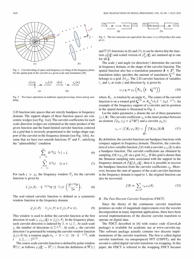
Fig. 1. Curvelet tiling of space and frequency (a) tiling of the frequency plane,(b) the spatial grid of the curvelet at a given scale and orientation [20].

Fig. 2. Two basic operations in multirate signal processing: down and up sam-pling.

2-D function into spaces that are strictly bandpass in frequencydomain. The support shapes of these function spaces are con-centric wedges [see Fig. 1(a)]. The curvelet coefficients for eachscale-direction wedges are estimated as the inner product of thegiven function and the band-limited curvelet function centeredon a grid that is inversely proportional to the wedge-shape sup-port of the curvelet in the frequency domain [see Fig. 1(b)]. As-sume that we have two smooth functions and , satisfyingthe “admissibility” condition

(6)

(7)

For each , the frequency window for the curveletfunction is given by

(8)

The real-valued curvelet function is defined as a symmetricwindow function in the frequency domain

(9)

This window is used to define the curvelet function at the firstdirection of scale , . In the frequency plane,each curvelet direction is indexed by . At each scale, the number of directions is . At scale , the curvelet

direction is generated by rotating the curvelet window functionby a rotation angle , with

.The coarse scale curvelet function is defined by polar window

as follows . From the definition of

Fig. 3. The two structures are equivalent: the same �� will produce the same��.

and functions in (6) and (7), it can be shown that the func-tion and scaled version of are summed up to onefor all .

The scale and angle (or direction) determine the curveletin frequency domain, or the shape of the curvelet function. Thespatial function also has a translation parameter . Thetranslation index specifies the amount of translation thatbelongs to a grid . The 2-D curvelet function of variables

and at scale and direction is given by

(10)

where is rotation by an angle . The center of the curveletfunction is on a rotated grid . Anexample of the frequency support of a curvelet and its positionin the spatial domain is illustrated in Fig. 1.

Let the index parameter denote the set of three parameters. The curvelet coefficient is the inner product between

an element and a curvelet

(11)

By definition, the curvelet functions are bandpass functions withcompact support in frequency domain. Therefore, the convolu-tion of a two-variable function with a curvelet is alsoa bandpass function. The curvelet coefficients are obtained bysampling on a grid . If this grid is denser thanthe Shannon sampling ratio associated with the support in thefrequency domain of , then it is possible to recoverthe bandpass function from the curvelet coefficients . More-over, because the sum of squares of the scale curvelet functionsin the frequency domain is equal to 1, the original function canalso be recovered:

(12)

B. The Fast Discrete Curvelet Transform (FDCT)

Since the theory of the continuous curvelet transformpromises an order of magnitude improvement over the waveletdecomposition in many important applications, there have beenseveral implementations of the discrete curvelet transform tooperate on digital data.

The FDCT described in [6] with source code (CurveLabpackage) is available for academic use at www.curvelet.org.This software package actually contains two discrete imple-mentations of the curvelet transform. The first is called digitalcurvelet transform via unequispaced FFT (USFFT), and thesecond is called digital curvelet transform via wrapping. In thispaper, the FDCT is referred to the wrapping FDCT because


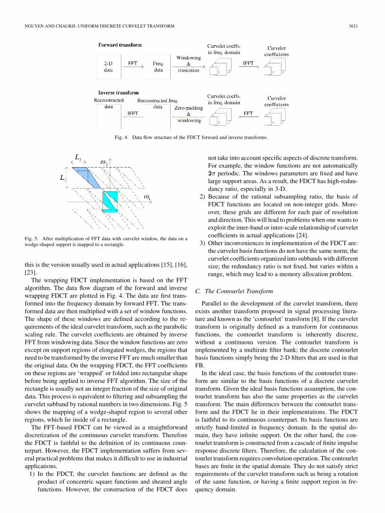
Fig. 4. Data flow structure of the FDCT forward and inverse transforms.

Fig. 5. After multiplication of FFT data with curvelet window, the data on awedge-shaped support is mapped to a rectangle.

this is the version usually used in actual applications [15], [16],[23].

The wrapping FDCT implementation is based on the FFTalgorithm. The data flow diagram of the forward and inversewrapping FDCT are plotted in Fig. 4. The data are first trans-formed into the frequency domain by forward FFT. The trans-formed data are then multiplied with a set of window functions.The shape of these windows are defined according to the re-quirements of the ideal curvelet transform, such as the parabolicscaling rule. The curvelet coefficients are obtained by inverseFFT from windowing data. Since the window functions are zeroexcept on support regions of elongated wedges, the regions thatneed to be transformed by the inverse FFT are much smaller thanthe original data. On the wrapping FDCT, the FFT coefficientson these regions are ‘wrapped’ or folded into rectangular shapebefore being applied to inverse FFT algorithm. The size of therectangle is usually not an integer fraction of the size of originaldata. This process is equivalent to filtering and subsampling thecurvelet subband by rational numbers in two dimensions. Fig. 5shows the mapping of a wedge-shaped region to several otherregions, which lie inside of a rectangle.

The FFT-based FDCT can be viewed as a straightforwarddiscretization of the continuous curvelet transform. Thereforethe FDCT is faithful to the definition of its continuous coun-terpart. However, the FDCT implementation suffers from sev-eral practical problems that makes it difficult to use in industrialapplications.

1) In the FDCT, the curvelet functions are defined as theproduct of concentric square functions and sheared anglefunctions. However, the construction of the FDCT does

not take into account specific aspects of discrete transform.For example, the window functions are not automatically

periodic. The windows parameters are fixed and havelarge support areas. As a result, the FDCT has high-redun-dancy ratio, especially in 3-D.

2) Because of the rational subsampling ratio, the basis ofFDCT functions are located on non-integer grids. More-over, these grids are different for each pair of resolutionand direction. This will lead to problems when one wants toexploit the inter-band or inter-scale relationship of curveletcoefficients in actual applications [24].

3) Other inconveniences in implementation of the FDCT are:the curvelet basis functions do not have the same norm; thecurvelet coefficients organized into subbands with differentsize; the redundancy ratio is not fixed, but varies within arange, which may lead to a memory allocation problem.

C. The Contourlet Transform

Parallel to the development of the curvelet transform, thereexists another transform proposed in signal processing litera-ture and known as the ‘contourlet’ transform [8]. If the curvelettransform is originally defined as a transform for continuousfunctions, the contourlet transform is inherently discrete,without a continuous version. The contourlet transform isimplemented by a multirate filter bank; the discrete contourletbasis functions simply being the 2-D filters that are used in thatFB.

In the ideal case, the basis functions of the contourlet trans-form are similar to the basis functions of a discrete curvelettransform. Given the ideal basis functions assumption, the con-tourlet transform has also the same properties as the curvelettransform. The main differences between the contourlet trans-form and the FDCT lie in their implementations. The FDCTis faithful to its continuous counterpart. Its basis functions arestrictly band-limited in frequency domain. In the spatial do-main, they have infinite support. On the other hand, the con-tourlet transform is constructed from a cascade of finite impulseresponse discrete filters. Therefore, the calculation of the con-tourlet transform requires convolution operation. The contourletbases are finite in the spatial domain. They do not satisfy strictrequirements of the curvelet transform such as being a rotationof the same function, or having a finite support region in fre-quency domain.


In the first construction of the contourlet transform [8], thecontourlet functions were not sharply localized in the frequencydomain. In a recent construction of the contourlet transform,this problem has been reduced [25], [26]. In the newly designedtransform, the actual contourlet functions are quite similar to thecurvelet functions in both spatial and frequency domain. There-fore, the two types of discrete transforms should have compa-rable performances in practical applications.

The contourlet transform, being implemented by a filter bank,is a digital-friendly transform. It has very low redundancy ratioand very fast implementation (faster than the FFT). The problemof this approach is that it is only an approximation of the curvelettransform, because the discrete basis contourlet function doesnot satisfy the criteria of a curvelet function. According to theconstruction of the curvelet transform, the basis functions inthe Fourier domain need to have a compact support, while thecontourlet basis functions, created by cascading digital filters,do not have this property.

IV. 2-D CURVELET WINDOW DEFINITION

Since this section contains rather involved notations, let usmake clear our objective. This section aims to construct a familyof smooth 2-D curvelet windows ( is an integer), de-noted as , . This family of smooth win-dows will be used in later sections in defining the curvelet func-tions in the frequency domain for the UDCT. The set of 2-Dfunctions satisfy the following criteria

• All windows functions are periodic in and . Inthe following, we limit the specification of to the

square.• The first window has a square-shape support and

zero outside region [Fig. 9(d)]. This functionis sometimes referred to as the lowpass window.

• The other windows have wedge-shaped supports[Fig. 9(a)].

• All are smooth functions, with compact support. Thefunction has value 1 in an “essential support” region andsmoothly transition to zero outside a compact support re-gion. The parameter and control the width of thesetransition regions.

• For the wedge-shaped support function, the widest part ofthe wedge must be smaller than a fractional of . In thecase illustrated in Fig. 9, the widest part of the wedge-shaped support of windows, , should be lessthan or equal to .

• The set of and form a partition ofunity, which means their sum equal to 1.

The construction of 2-D window functions are dividedin to several steps. We first define a function which hasa smooth transition from 0 to 1. Based on the function,a set of 2 smooth concentric square windows and a set ofangle windows are created. The parameter controls the widthof the transition regions of concentric square windows, whileparameter controls the transition regions of angle windows.The square-shape support is created from the product oftwo 1-D functions. The wedge-shaped supports are con-structed as the products of a concentric square passband windowand the set of angle windows.

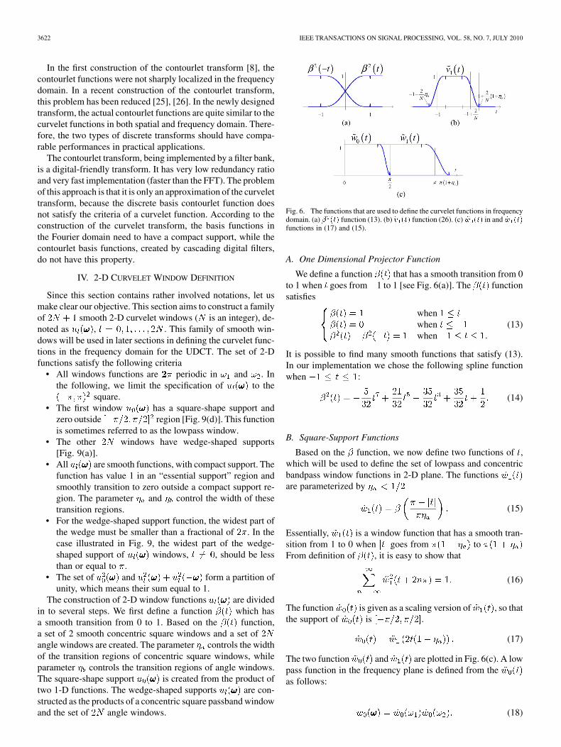
Fig. 6. The functions that are used to define the curvelet functions in frequencydomain. (a) � �� function (13). (b) �� function (26). (c) �� in and �� functions in (17) and (15).

A. One Dimensional Projector Function

We define a function that has a smooth transition from 0to 1 when goes from 1 to 1 [see Fig. 6(a)]. The functionsatisfies

whenwhenwhen

(13)

It is possible to find many smooth functions that satisfy (13).In our implementation we chose the following spline functionwhen :

(14)

B. Square-Support Functions

Based on the function, we now define two functions of ,which will be used to define the set of lowpass and concentricbandpass window functions in 2-D plane. The functionsare parameterized by

(15)

Essentially, is a window function that has a smooth tran-sition from 1 to 0 when goes from toFrom definition of , it is easy to show that

(16)

The function is given as a scaling version of , so thatthe support of is .

(17)

The two function and are plotted in Fig. 6(c). A lowpass function in the frequency plane is defined from theas follows:

(18)


The is zero outside the square . We nowdefine based on lowpass window and in(15)

(19)

Following the definitions of and in (18) and (19)

(20)

This is because with , when[see Fig. 6(c)]. Therefore, .

Because our windows will be used as the discrete curveletfunctions in frequency domain, they have to be periodic. Thefunction is periodized as follows:

(21)

A 3-D view of is in Fig. 9(d). On the square, the2-D function has a square support . Moreover, bythe scaling relationship in (17), when

. If , wehave the following relationship:

whenwhen

(22)The function corresponds to a lowpass discrete filter, andthe function is a smooth bandpass function with concen-tric square support. Intuitively, their sum of squares is equal toone.

(23)

(24)

(25)

Equation (23) is obtained from (21) and the fact thatare not overlapping. The next two steps are results of (20)

and (16).

C. Angle Polar Functions

A set of polar angle functions is defined in this section.Similar to the angle function in continuous case [ in (7)],their squares are summed up to one. However, since the newangle functions are defined for discrete frequency plane, therotation relationship between two functions will be replaced bythe shearing relationship.

Assume that the angle functions that need to be defined is ,with essential support in the range . First, we needto define intermediary functions , :

(26)

(27)

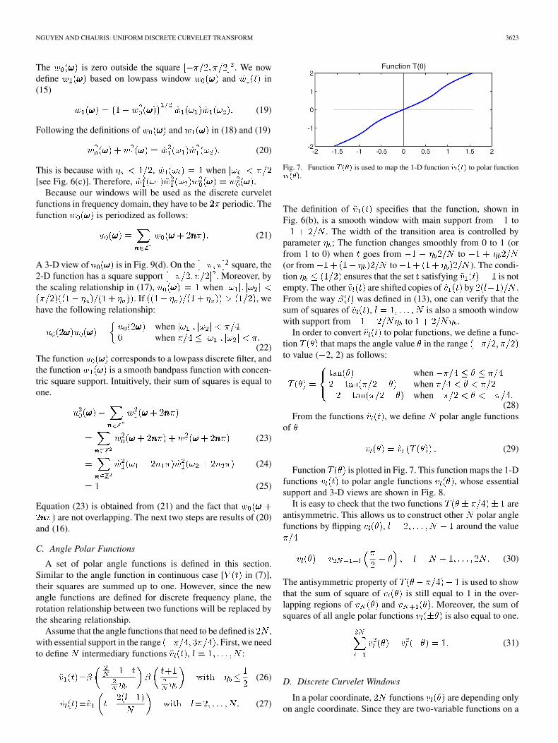
Fig. 7. Function � �� is used to map the 1-D function �� to polar function� ��.

The definition of specifies that the function, shown inFig. 6(b), is a smooth window with main support from 1 to

. The width of the transition area is controlled byparameter ; The function changes smoothly from 0 to 1 (orfrom 1 to 0) when goes from to(or from to ). The condi-tion ensures that the set satisfying is notempty. The other are shifted copies of by .From the way was defined in (13), one can verify that thesum of squares of , is also a smooth windowwith support from to .

In order to convert to polar functions, we define a func-tion that maps the angle value in the rangeto value ( 2, 2) as follows:

whenwhenwhen

(28)From the functions , we define polar angle functions

of

(29)

Function is plotted in Fig. 7. This function maps the 1-Dfunctions to polar angle functions , whose essentialsupport and 3-D views are shown in Fig. 8.

It is easy to check that the two functions areantisymmetric. This allows us to construct other polar anglefunctions by flipping , around the value

(30)

The antisymmetric property of is used to showthat the sum of square of is still equal to 1 in the over-lapping regions of and . Moreover, the sum ofsquares of all angle polar functions is also equal to one.

(31)

D. Discrete Curvelet Windows

In a polar coordinate, functions are depending onlyon angle coordinate. Since they are two-variable functions on a


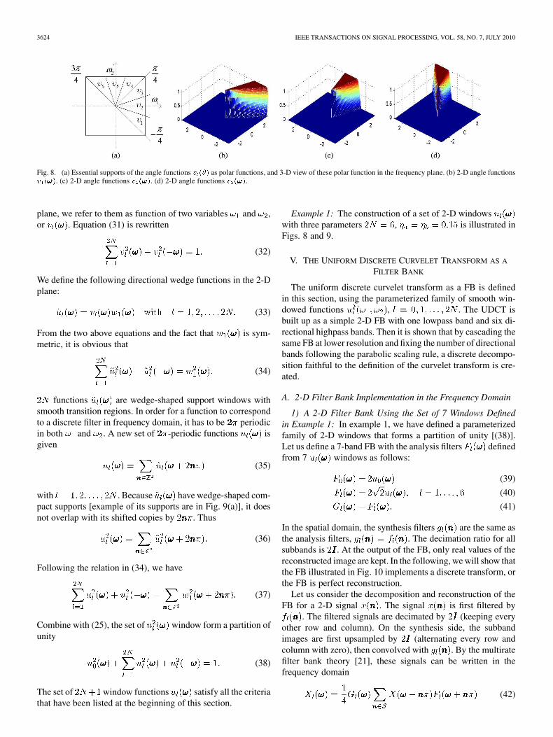
Fig. 8. (a) Essential supports of the angle functions � �� as polar functions, and 3-D view of these polar function in the frequency plane. (b) 2-D angle functions� ��. (c) 2-D angle functions � ��. (d) 2-D angle functions � ��.

plane, we refer to them as function of two variables and ,or . Equation (31) is rewritten

(32)

We define the following directional wedge functions in the 2-Dplane:

(33)

From the two above equations and the fact that is sym-metric, it is obvious that

(34)

functions are wedge-shaped support windows withsmooth transition regions. In order for a function to correspondto a discrete filter in frequency domain, it has to be periodicin both and . A new set of -periodic functions isgiven

(35)

with . Because have wedge-shaped com-pact supports [example of its supports are in Fig. 9(a)], it doesnot overlap with its shifted copies by . Thus

(36)

Following the relation in (34), we have

(37)

Combine with (25), the set of window form a partition ofunity

(38)

The set of window functions satisfy all the criteriathat have been listed at the beginning of this section.

Example 1: The construction of a set of 2-D windowswith three parameters , is illustrated inFigs. 8 and 9.

V. THE UNIFORM DISCRETE CURVELET TRANSFORM AS A

FILTER BANK

The uniform discrete curvelet transform as a FB is definedin this section, using the parameterized family of smooth win-dowed functions , . The UDCT isbuilt up as a simple 2-D FB with one lowpass band and six di-rectional highpass bands. Then it is shown that by cascading thesame FB at lower resolution and fixing the number of directionalbands following the parabolic scaling rule, a discrete decompo-sition faithful to the definition of the curvelet transform is cre-ated.

A. 2-D Filter Bank Implementation in the Frequency Domain

1) A 2-D Filter Bank Using the Set of 7 Windows Definedin Example 1: In example 1, we have defined a parameterizedfamily of 2-D windows that forms a partition of unity [(38)].Let us define a 7-band FB with the analysis filters definedfrom 7 windows as follows:

(39)

(40)

(41)

In the spatial domain, the synthesis filters are the same asthe analysis filters, . The decimation ratio for allsubbands is . At the output of the FB, only real values of thereconstructed image are kept. In the following, we will show thatthe FB illustrated in Fig. 10 implements a discrete transform, orthe FB is perfect reconstruction.

Let us consider the decomposition and reconstruction of theFB for a 2-D signal . The signal is first filtered by

. The filtered signals are decimated by (keeping everyother row and column). On the synthesis side, the subbandimages are first upsampled by (alternating every row andcolumn with zero), then convolved with . By the multiratefilter bank theory [21], these signals can be written in thefrequency domain

(42)


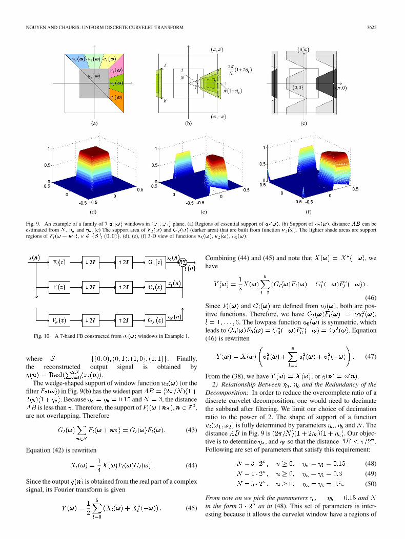
Fig. 9. An example of a family of 7 � �� windows in �� plane. (a) Regions of essential support of � ��. (b) Support of � ��, distance �� can beestimated from � , � and � . (c) The support area of � �� and �� (darker area) that are built from function � ��. The lighter shade areas are supportregions of � �� , � �� . (d), (e), (f) 3-D view of functions � ��, � ��, � ��.

Fig. 10. A 7-band FB constructed from � �� windows in Example 1.

where . Finally,the reconstructed output signal is obtained by

.The wedge-shaped support of window function (or the

filter ) in Fig. 9(b) has the widest part. Because and , the distance

is less than . Therefore, the support of , ,are not overlapping. Therefore

(43)

Equation (42) is rewritten

(44)

Since the output is obtained from the real part of a complexsignal, its Fourier transform is given

(45)

Combining (44) and (45) and note that , wehave

(46)Since and are defined from , both are pos-itive functions. Therefore, we have ,

. The lowpass function is symmetric, whichleads to . Equation(46) is rewritten

(47)

From the (38), we have , or .2) Relationship Between , and the Redundancy of the

Decomposition: In order to reduce the overcomplete ratio of adiscrete curvelet decomposition, one would need to decimatethe subband after filtering. We limit our choice of decimationratio to the power of 2. The shape of support of a function

is fully determined by parameters , and . Thedistance in Fig. 9 is . Our objec-tive is to determine , and so that the distance .Following are set of parameters that satisfy this requirement:

(48)

(49)

(50)

From now on we pick the parameters andin the form as in (48). This set of parameters is inter-esting because it allows the curvelet window have a regions of


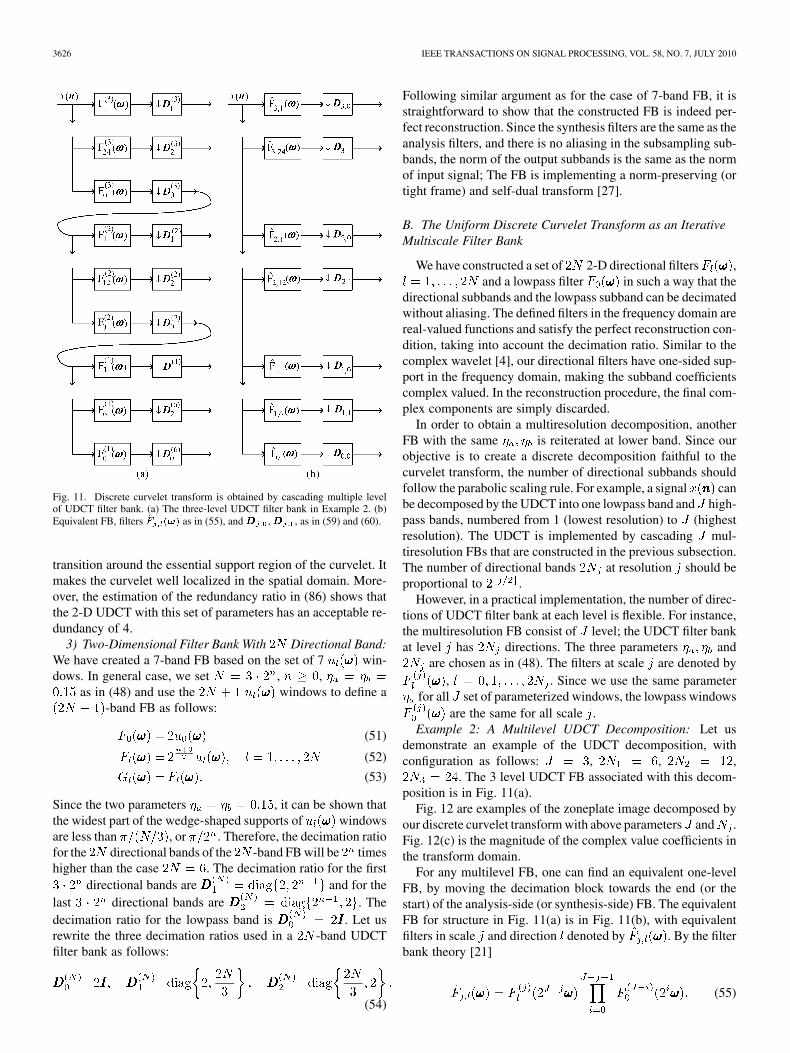
Fig. 11. Discrete curvelet transform is obtained by cascading multiple levelof UDCT filter bank. (a) The three-level UDCT filter bank in Example 2. (b)Equivalent FB, filters �� as in (55), and�� ,�� , as in (59) and (60).

transition around the essential support region of the curvelet. Itmakes the curvelet well localized in the spatial domain. More-over, the estimation of the redundancy ratio in (86) shows thatthe 2-D UDCT with this set of parameters has an acceptable re-dundancy of 4.

3) Two-Dimensional Filter Bank With Directional Band:We have created a 7-band FB based on the set of 7 win-dows. In general case, we set , ,

as in (48) and use the windows to define a-band FB as follows:

(51)

(52)

(53)

Since the two parameters , it can be shown thatthe widest part of the wedge-shaped supports of windowsare less than , or . Therefore, the decimation ratiofor the directional bands of the -band FB will be timeshigher than the case . The decimation ratio for the first

directional bands are and for thelast directional bands are . Thedecimation ratio for the lowpass band is . Let usrewrite the three decimation ratios used in a -band UDCTfilter bank as follows:

(54)

Following similar argument as for the case of 7-band FB, it isstraightforward to show that the constructed FB is indeed per-fect reconstruction. Since the synthesis filters are the same as theanalysis filters, and there is no aliasing in the subsampling sub-bands, the norm of the output subbands is the same as the normof input signal; The FB is implementing a norm-preserving (ortight frame) and self-dual transform [27].

B. The Uniform Discrete Curvelet Transform as an IterativeMultiscale Filter Bank

We have constructed a set of 2-D directional filters ,and a lowpass filter in such a way that the

directional subbands and the lowpass subband can be decimatedwithout aliasing. The defined filters in the frequency domain arereal-valued functions and satisfy the perfect reconstruction con-dition, taking into account the decimation ratio. Similar to thecomplex wavelet [4], our directional filters have one-sided sup-port in the frequency domain, making the subband coefficientscomplex valued. In the reconstruction procedure, the final com-plex components are simply discarded.

In order to obtain a multiresolution decomposition, anotherFB with the same is reiterated at lower band. Since ourobjective is to create a discrete decomposition faithful to thecurvelet transform, the number of directional subbands shouldfollow the parabolic scaling rule. For example, a signal canbe decomposed by the UDCT into one lowpass band and high-pass bands, numbered from 1 (lowest resolution) to (highestresolution). The UDCT is implemented by cascading mul-tiresolution FBs that are constructed in the previous subsection.The number of directional bands at resolution should beproportional to .

However, in a practical implementation, the number of direc-tions of UDCT filter bank at each level is flexible. For instance,the multiresolution FB consist of level; the UDCT filter bankat level has directions. The three parameters and

are chosen as in (48). The filters at scale are denoted by, . Since we use the same parameter

for all set of parameterized windows, the lowpass windowsare the same for all scale .

Example 2: A Multilevel UDCT Decomposition: Let usdemonstrate an example of the UDCT decomposition, withconfiguration as follows: , , ,

. The 3 level UDCT FB associated with this decom-position is in Fig. 11(a).

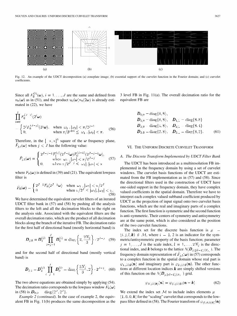
Fig. 12 are examples of the zoneplate image decomposed byour discrete curvelet transform with above parameters and .Fig. 12(c) is the magnitude of the complex value coefficients inthe transform domain.

For any multilevel FB, one can find an equivalent one-levelFB, by moving the decimation block towards the end (or thestart) of the analysis-side (or synthesis-side) FB. The equivalentFB for structure in Fig. 11(a) is in Fig. 11(b), with equivalentfilters in scale and direction denoted by . By the filterbank theory [21]

(55)


Fig. 12. An example of the UDCT decomposition (a) zoneplate image; (b) essential support of the curvelet function in the Fourier domain; and (c) curveletcoefficients.

Since all , are the same and defined fromas in (51), and the product is already esti-

mated in (22), we have

whenwhen

(56)

Therefore, in the square of the frequency plane,when has the following value:

(57)

where is defined in (39) and (21). The equivalent lowpassfilter is

whenwhen

(58)We have determined the equivalent curvelet filters of an iteratedUDCT filter bank in (57) and (58) by pushing all the analysisfilters to the left and all the decimation blocks to the right onthe analysis side. Associated with the equivalent filters are theoverall decimation ratio, which are the product of all decimationblocks along the branch of the iterative FB. The decimation ratiofor the first half of directional band (mostly horizontal band) is

(59)

and for the second half of directional band (mostly verticalband) is

(60)

The two above equations are obtained simply by applying (54).The decimation ratio corresponds to the lowpass windowin (58) is .

Example 2 (continued). In the case of example 2, the equiv-alent FB in Fig. 11(b) produces the same decomposition as the

3 level FB in Fig. 11(a). The overall decimation ratio for theequivalent FB are

(61)

VI. THE UNIFORM DISCRETE CURVELET TRANSFORM

A. The Discrete Transform Implemented by UDCT Filter Bank

The UDCT has been introduced as a multiresolution FB im-plemented in the frequency domain by using a set of curveletwindows. The curvelet basis functions of the UDCT are esti-mated from the FB implementation as in (57) and (58). Sincethe directional filters used in the construction of UDCT haveone-sided support in the frequency domain, they have complexvalued coefficients in the spatial domain. Therefore we have tointerpret each complex valued subband coefficient produced byUDCT as the projection of input signal onto two curvelet basisfunctions, which are the real and imaginary parts of a complexfunction. The first function is symmetric and the second functionis anti-symmetric. Their centers of symmetry and antisymmetryare at the same point, which is also considered as the positionof the two curvelet functions.

The index set for the discrete basis function is, where , 2 is an indicator for the sym-

metric/antisymmetric property of the basis function; parameteris the scale index, is the direc-

tional index, and belongs to the lattice . Thefrequency domain representation of in (57) correspondsto a complex function in the spatial domain whose real part is

and imaginary part is . The other func-tions at different location indices are simply shifted versionsof this function on the grid.

(62)

We extend the index set to include index elementsfor the “scaling” curvelet that corresponds to the low-

pass filter defined in (58). The Fourier transform of


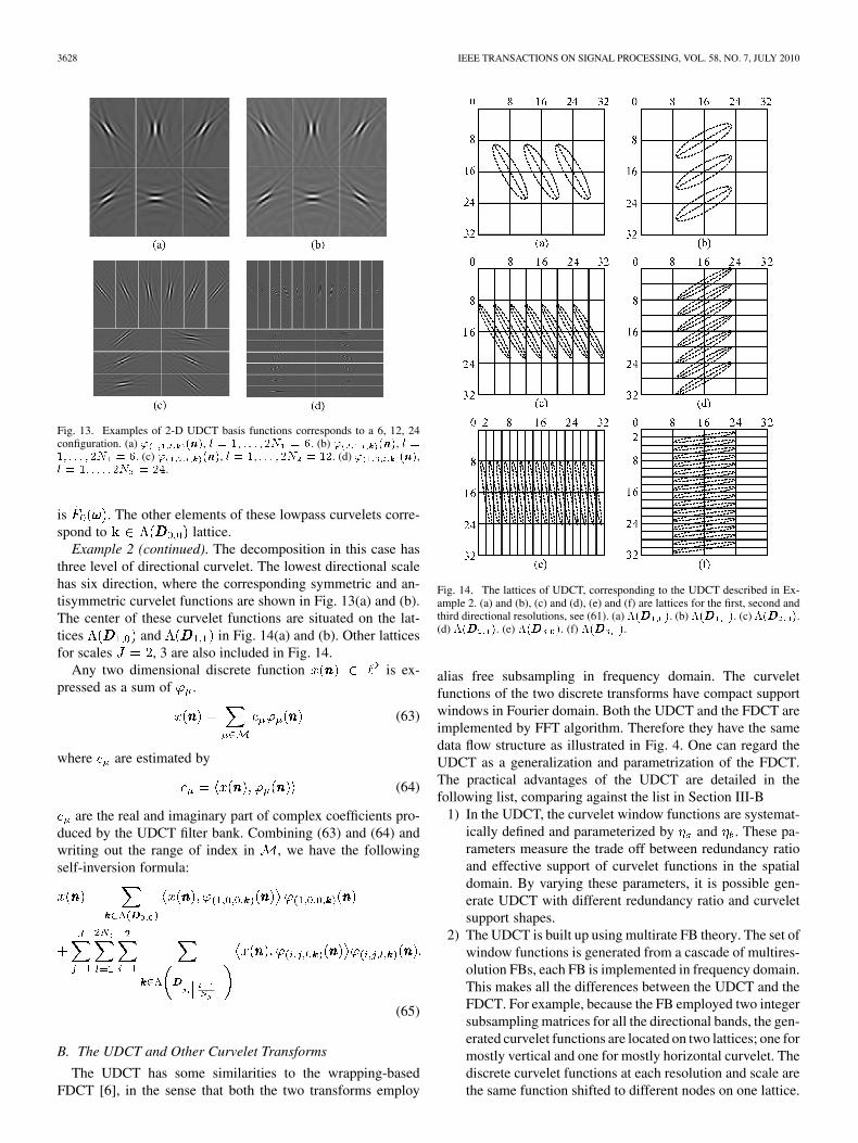
Fig. 13. Examples of 2-D UDCT basis functions corresponds to a 6, 12, 24configuration. (a) � ��, � � �� . (b) � ��, � �� . (c) � ��, � � �� . (d) � ��,� � �� .

is . The other elements of these lowpass curvelets corre-spond to lattice.

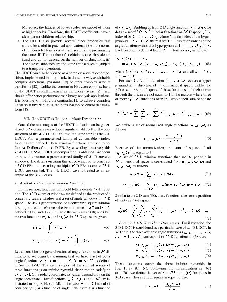
Example 2 (continued). The decomposition in this case hasthree level of directional curvelet. The lowest directional scalehas six direction, where the corresponding symmetric and an-tisymmetric curvelet functions are shown in Fig. 13(a) and (b).The center of these curvelet functions are situated on the lat-tices and in Fig. 14(a) and (b). Other latticesfor scales , 3 are also included in Fig. 14.

Any two dimensional discrete function is ex-pressed as a sum of .

(63)

where are estimated by

(64)

are the real and imaginary part of complex coefficients pro-duced by the UDCT filter bank. Combining (63) and (64) andwriting out the range of index in , we have the followingself-inversion formula:

(65)

B. The UDCT and Other Curvelet Transforms

The UDCT has some similarities to the wrapping-basedFDCT [6], in the sense that both the two transforms employ

Fig. 14. The lattices of UDCT, corresponding to the UDCT described in Ex-ample 2. (a) and (b), (c) and (d), (e) and (f) are lattices for the first, second andthird directional resolutions, see (61). (a) �� . (b) �� . (c) �� .(d) �� . (e) �� . (f) �� .

alias free subsampling in frequency domain. The curveletfunctions of the two discrete transforms have compact supportwindows in Fourier domain. Both the UDCT and the FDCT areimplemented by FFT algorithm. Therefore they have the samedata flow structure as illustrated in Fig. 4. One can regard theUDCT as a generalization and parametrization of the FDCT.The practical advantages of the UDCT are detailed in thefollowing list, comparing against the list in Section III-B

1) In the UDCT, the curvelet window functions are systemat-ically defined and parameterized by and . These pa-rameters measure the trade off between redundancy ratioand effective support of curvelet functions in the spatialdomain. By varying these parameters, it is possible gen-erate UDCT with different redundancy ratio and curveletsupport shapes.

2) The UDCT is built up using multirate FB theory. The set ofwindow functions is generated from a cascade of multires-olution FBs, each FB is implemented in frequency domain.This makes all the differences between the UDCT and theFDCT. For example, because the FB employed two integersubsampling matrices for all the directional bands, the gen-erated curvelet functions are located on two lattices; one formostly vertical and one for mostly horizontal curvelet. Thediscrete curvelet functions at each resolution and scale arethe same function shifted to different nodes on one lattice.


Moreover, the lattices of lower scales are subset of thoseat higher scales. Therefore, the UDCT coefficients have aclear parent-children relationship.

3) The UDCT also provide several other properties thatshould be useful in practical applications: i) All the normsof the curvelet functions at each scale are approximatelythe same. ii) The number of coefficients at each scale arefixed and do not depend on the number of directions. iii)The size of subbands are the same for each scale (subjectto a transpose operation).

The UDCT can also be viewed as a complex wavelet decompo-sition, implemented by filter bank, in the same way as shiftablecomplex directional pyramid [19] or other complex wavelettransforms [28]. Unlike the contourlet FB, each complex bandof the UDCT is shift invariant in the energy sense [29], andshould offer better performances in image analysis applications.It is possible to modify the contourlet FB to achieve completelinear shift invariant as in the nonsubsampled contourlet trans-form [18].

VII. THE UDCT IN THREE OR MORE DIMENSIONS

One of the advantages of the UDCT is that it can be gener-alized to -dimensions without significant difficulty. The con-struction of the -D UDCT follows the same steps as the 2-DUDCT. First a parameterized family of variable windowfunctions are defined. These window functions are used to de-fine -D filters for a -D FB. By cascading iteratively this

-D FB, a -D UDCT decomposition is obtained. We focuson how to construct a parameterized family of -D curveletwindows. The details on using this set of windows to constructa -D FB, and cascading multiple -D FBs to create -DUDCT are omitted. The 3-D UDCT case is treated as an ex-ample of the -D cases.

A. A Set of -D Curvelet Window Functions

In this section, functions with bold letters denote -D func-tion. The -D curvelet windows are defined as the product of aconcentric square window and a set of angle windows in -Dspace. The -D generalization of a concentric square windowis straightforward. We reuse the two functions anddefined in (15) and (17). Similar to the 2-D case in (18) and (19),the two functions and in -D space are given

(66)

(67)

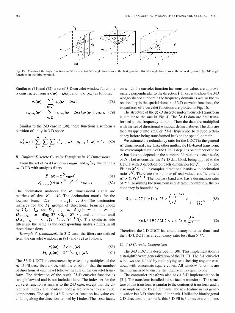
Let us consider the generalization of angle functions in di-mensions. We begin by assuming that we have a set of polarangle functions , , as definedin Section IV-C. The main support of the sum of square ofthese functions is an infinite pyramid shape region satisfying

; On a polar coordinate, its values depend only on theangle coordinate. Three functions , and are il-lustrated in Fig. 8(b), (c), (d), in the case . Instead ofconsidering as a function of angle , we write it as a function

of . Building up from 2-D angle function , wedefine a set of polar functions on -D space ,indexed by , where is the index of the hyper-pyramid, ; the rest are direction indices of theangle function within that hyperpyramid, .Each function is defined from functions as follows:

(68)

where and all ,.

For each , function covers a hyperpyramid in direction of dimensional space. Unlike the2-D case, the sum of square of these functions and their mirrorthrough the origin are not equal to 1 in the regions where threeor more functions overlap. Denote their sum of squareas

(69)

We define a set of normalized angle functions asfollows

(70)

Because of the normalization, the sum of square of allis equal to 1.

A set of -D window functions that are periodic indimensional space is constructed from , and

as follows:

(71)

(72)

Similar to the 2-D case (38), these functions also form a partitionof unity in -D space

(73)Example 3, UDCT in Three Dimensions: For illustration, the

3-D UDCT is considered as a particular case of -D UDCT. In3-D case, the three-variable angle functions ,

, correspond to -D functions in (68), are

(74)

(75)

(76)

These functions cover the three infinite pyramids inFig. 15(a), (b), (c). Following the normalization in (69)and (70), we define the set of functions in3-D space whose sum of square is equal to one:

(77)


Fig. 15. Construct the angle functions in 3-D space. (a) 3-D angle functions in the first pyramid. (b) 3-D angle functions in the second pyramid. (c) 3-D anglefunctions in the third pyramid.

Similar to (71) and (72), a set of 3-D curvelet window functionsis constructed from , , and as follows:

(78)

(79)

Similar to the 2-D case in (38), these functions also form apartition of unity in 3-D space

(80)

B. Uniform Discrete Curvelet Transform in Dimensions

From the set of -D windows and , we define a-D FB with analysis filters

(81)

(82)

The decimation matrices for dimensional signal arematrices of size . The decimation matrix for thelowpass branch ; The decimationmatrices for the groups of directional branches indexby are ,

, and continue until. The synthesis side

filters are the same as the corresponding analysis filters in allthree dimensions.

Example 3, (continued). In 3-D case, the filters are definedfrom the curvelet windows in (81) and (82) as follows:

(83)

(84)

The -D UDCT is constructed by cascading multiples of the-D FB described above, with the condition that the number

of directions at each level follows the rule of the curvelet trans-form. The derivation of the result -D curvelet function isstraightforward and is not included here. The index set for thecurvelet function is similar to the 2-D case, except that the di-rectional index and position index are now vectors withcomponents. The spatial -D curvelet function has value os-cillating along the direction defined by index. The isosurfaces,

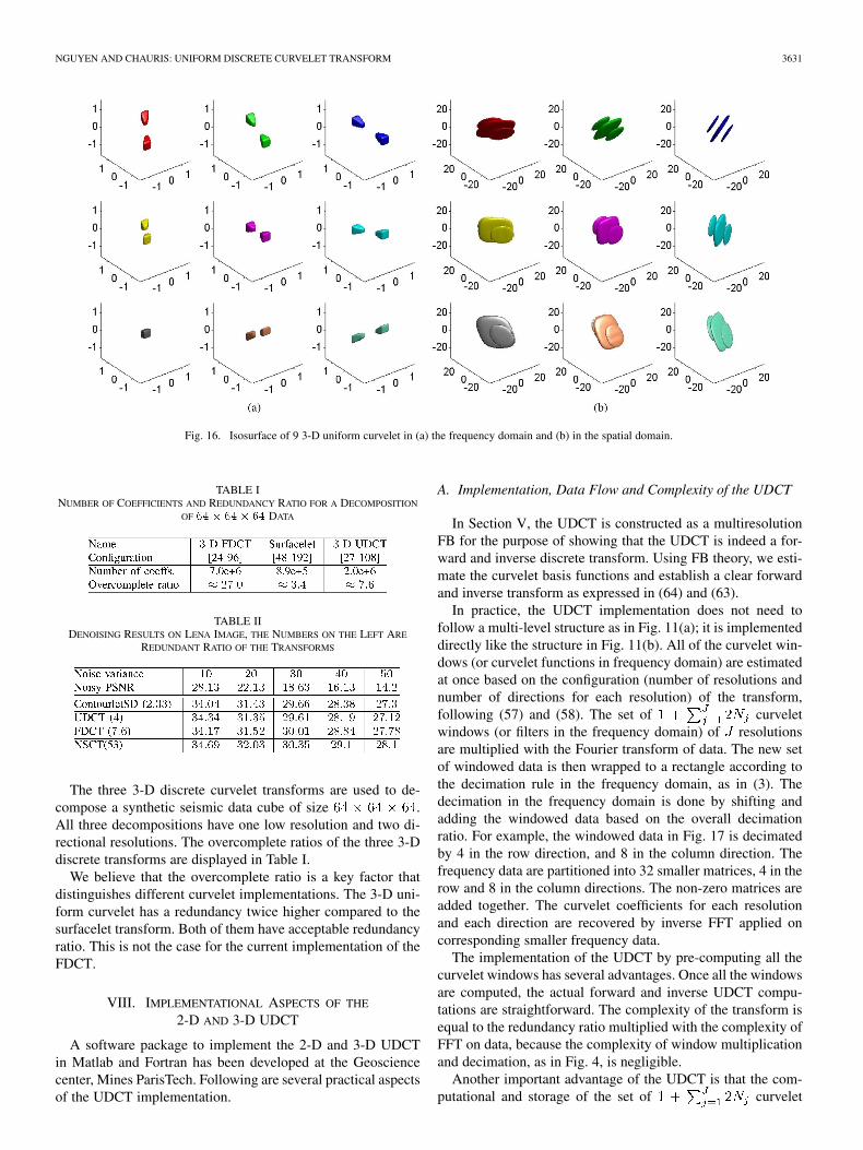
on which the curvelet function has constant value, are approxi-mately perpendicular to the direction . In order to show the 3-Dwedge-shaped support in the frequency domain as well as the di-rectionality in the spatial domain of 3-D curvelet functions, theisosurfaces of 9 curvelet functions are plotted in Fig. 16.

The structure of the -D discrete uniform curvelet transformis similar to the one in Fig. 4. The -D data are first trans-formed to the frequency domain. Then the data are multipliedwith the set of directional windows defined above. The data arethen wrapped into smaller -D hypercube to reduce redun-dancy before being transformed back to the spatial domain.

We estimate the redundancy ratio for the UDCT in the generaldimensional case. Like other multiscale FB-based transform,

the overcomplete ratio of the UDCT depends on number of scale, but does not depend on the number of directions at each scale,

or . Let us consider the -D data block being applied to theUDCT with 3 direction on each dimension (or ). TheFB has complex directional bands with decimationratio . Therefore the number of real-valued coefficients is

. The lowpass band also has a decimation ratioof . Assuming the transform is reiterated indefinitely, the re-dundancy is bounded by

(85)

or

(86)

Therefore, the 2-D UDCT has a redundancy ratio less than 4 andthe 3-D UDCT has a redundancy ratio less than 54/7.

C. 3-D Curvelet Comparison

The 3-D FDCT is described in [30]. This implementation isa straightforward generalization of the FDCT. The 3-D curveletwindows are defined by multiplying two shearing angular win-dows with concentric square cubes. All window functions arethen normalized to ensure that their sum is equal to one.

The contourlet transform also has a 3-D implementation in[31]. The transform is called the surfacelet transform. The struc-ture of this transform is similar to the contourlet transform and isalso implemented by a filter bank. The new feature in this gener-alization is a 3-D directional filter bank. Unlike the biorthogonal2-D directional filter bank, this 3-D FB is 3 times overcomplete.


Fig. 16. Isosurface of 9 3-D uniform curvelet in (a) the frequency domain and (b) in the spatial domain.

TABLE INUMBER OF COEFFICIENTS AND REDUNDANCY RATIO FOR A DECOMPOSITION

OF �� DATA

TABLE IIDENOISING RESULTS ON LENA IMAGE, THE NUMBERS ON THE LEFT ARE

REDUNDANT RATIO OF THE TRANSFORMS

The three 3-D discrete curvelet transforms are used to de-compose a synthetic seismic data cube of size .All three decompositions have one low resolution and two di-rectional resolutions. The overcomplete ratios of the three 3-Ddiscrete transforms are displayed in Table I.

We believe that the overcomplete ratio is a key factor thatdistinguishes different curvelet implementations. The 3-D uni-form curvelet has a redundancy twice higher compared to thesurfacelet transform. Both of them have acceptable redundancyratio. This is not the case for the current implementation of theFDCT.

VIII. IMPLEMENTATIONAL ASPECTS OF THE

2-D AND 3-D UDCT

A software package to implement the 2-D and 3-D UDCTin Matlab and Fortran has been developed at the Geosciencecenter, Mines ParisTech. Following are several practical aspectsof the UDCT implementation.

A. Implementation, Data Flow and Complexity of the UDCT

In Section V, the UDCT is constructed as a multiresolutionFB for the purpose of showing that the UDCT is indeed a for-ward and inverse discrete transform. Using FB theory, we esti-mate the curvelet basis functions and establish a clear forwardand inverse transform as expressed in (64) and (63).

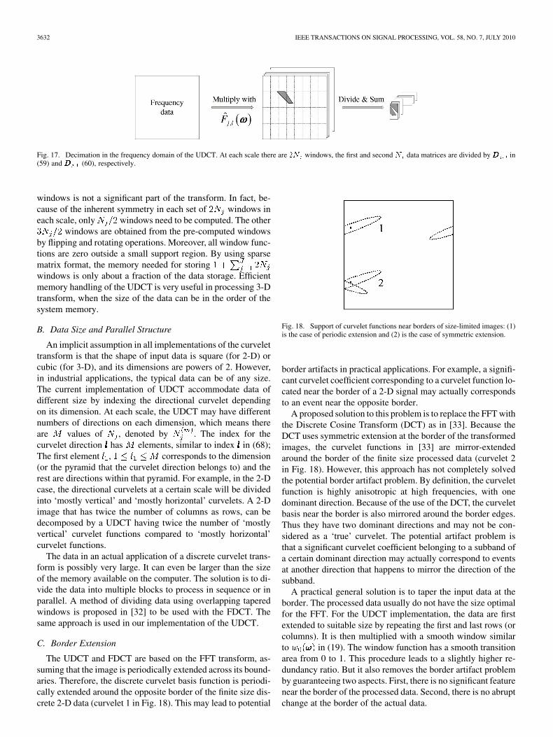
In practice, the UDCT implementation does not need tofollow a multi-level structure as in Fig. 11(a); it is implementeddirectly like the structure in Fig. 11(b). All of the curvelet win-dows (or curvelet functions in frequency domain) are estimatedat once based on the configuration (number of resolutions andnumber of directions for each resolution) of the transform,following (57) and (58). The set of curveletwindows (or filters in the frequency domain) of resolutionsare multiplied with the Fourier transform of data. The new setof windowed data is then wrapped to a rectangle according tothe decimation rule in the frequency domain, as in (3). Thedecimation in the frequency domain is done by shifting andadding the windowed data based on the overall decimationratio. For example, the windowed data in Fig. 17 is decimatedby 4 in the row direction, and 8 in the column direction. Thefrequency data are partitioned into 32 smaller matrices, 4 in therow and 8 in the column directions. The non-zero matrices areadded together. The curvelet coefficients for each resolutionand each direction are recovered by inverse FFT applied oncorresponding smaller frequency data.

The implementation of the UDCT by pre-computing all thecurvelet windows has several advantages. Once all the windowsare computed, the actual forward and inverse UDCT compu-tations are straightforward. The complexity of the transform isequal to the redundancy ratio multiplied with the complexity ofFFT on data, because the complexity of window multiplicationand decimation, as in Fig. 4, is negligible.

Another important advantage of the UDCT is that the com-putational and storage of the set of curvelet


Fig. 17. Decimation in the frequency domain of the UDCT. At each scale there are �� windows, the first and second � data matrices are divided by�� in(59) and �� (60), respectively.

windows is not a significant part of the transform. In fact, be-cause of the inherent symmetry in each set of windows ineach scale, only windows need to be computed. The other

windows are obtained from the pre-computed windowsby flipping and rotating operations. Moreover, all window func-tions are zero outside a small support region. By using sparsematrix format, the memory needed for storingwindows is only about a fraction of the data storage. Efficientmemory handling of the UDCT is very useful in processing 3-Dtransform, when the size of the data can be in the order of thesystem memory.

B. Data Size and Parallel Structure

An implicit assumption in all implementations of the curvelettransform is that the shape of input data is square (for 2-D) orcubic (for 3-D), and its dimensions are powers of 2. However,in industrial applications, the typical data can be of any size.The current implementation of UDCT accommodate data ofdifferent size by indexing the directional curvelet dependingon its dimension. At each scale, the UDCT may have differentnumbers of directions on each dimension, which means thereare values of , denoted by . The index for thecurvelet direction has elements, similar to index in (68);The first element , corresponds to the dimension(or the pyramid that the curvelet direction belongs to) and therest are directions within that pyramid. For example, in the 2-Dcase, the directional curvelets at a certain scale will be dividedinto ‘mostly vertical’ and ‘mostly horizontal’ curvelets. A 2-Dimage that has twice the number of columns as rows, can bedecomposed by a UDCT having twice the number of ‘mostlyvertical’ curvelet functions compared to ‘mostly horizontal’curvelet functions.

The data in an actual application of a discrete curvelet trans-form is possibly very large. It can even be larger than the sizeof the memory available on the computer. The solution is to di-vide the data into multiple blocks to process in sequence or inparallel. A method of dividing data using overlapping taperedwindows is proposed in [32] to be used with the FDCT. Thesame approach is used in our implementation of the UDCT.

C. Border Extension

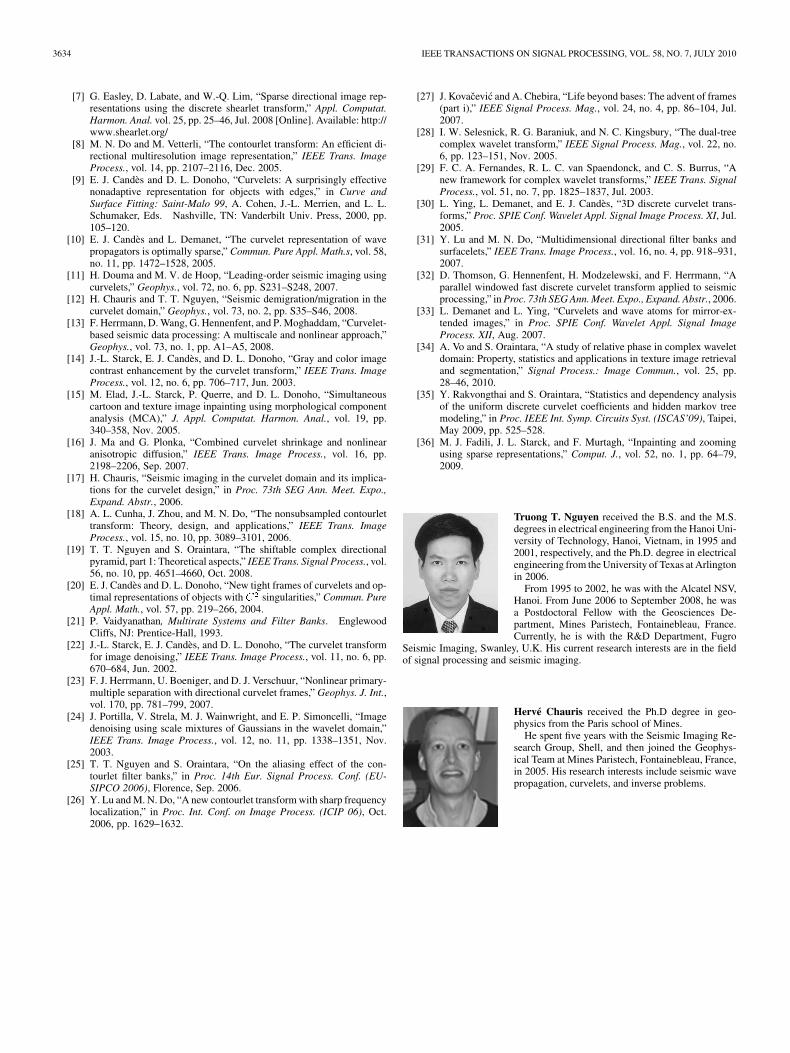
The UDCT and FDCT are based on the FFT transform, as-suming that the image is periodically extended across its bound-aries. Therefore, the discrete curvelet basis function is periodi-cally extended around the opposite border of the finite size dis-crete 2-D data (curvelet 1 in Fig. 18). This may lead to potential

Fig. 18. Support of curvelet functions near borders of size-limited images: (1)is the case of periodic extension and (2) is the case of symmetric extension.

border artifacts in practical applications. For example, a signifi-cant curvelet coefficient corresponding to a curvelet function lo-cated near the border of a 2-D signal may actually correspondsto an event near the opposite border.

A proposed solution to this problem is to replace the FFT withthe Discrete Cosine Transform (DCT) as in [33]. Because theDCT uses symmetric extension at the border of the transformedimages, the curvelet functions in [33] are mirror-extendedaround the border of the finite size processed data (curvelet 2in Fig. 18). However, this approach has not completely solvedthe potential border artifact problem. By definition, the curveletfunction is highly anisotropic at high frequencies, with onedominant direction. Because of the use of the DCT, the curveletbasis near the border is also mirrored around the border edges.Thus they have two dominant directions and may not be con-sidered as a ‘true’ curvelet. The potential artifact problem isthat a significant curvelet coefficient belonging to a subband ofa certain dominant direction may actually correspond to eventsat another direction that happens to mirror the direction of thesubband.

A practical general solution is to taper the input data at theborder. The processed data usually do not have the size optimalfor the FFT. For the UDCT implementation, the data are firstextended to suitable size by repeating the first and last rows (orcolumns). It is then multiplied with a smooth window similarto in (19). The window function has a smooth transitionarea from 0 to 1. This procedure leads to a slightly higher re-dundancy ratio. But it also removes the border artifact problemby guaranteeing two aspects. First, there is no significant featurenear the border of the processed data. Second, there is no abruptchange at the border of the actual data.


Fig. 19. Image inpainting application of the UDCT. (a) Lena image with 80%number of pixels missing �� . (b) inpainted Lena image byalgorithm in [36] with UDCT dictionary, �� .

IX. NUMERICAL RESULTS

In this section, we present several simple experiments usingthe UDCT. The parameters and receive values as in (48).The UDCT has also been used in other image processing appli-cations [34], [35].

A. Application of the UDCT to Image Inpainting

Here we demonstrate the use of the UDCT in the image in-painting problem. We use the image inpainting algorithm in[36], publicly available with a Matlab implementation. The in-painting method is designed for filling missing pixels in images;The main assumption of the method is that the image consistsof several layers and all layers have sparse representations inincoherent dictionaries. We assume that the testing image has asparse representation in the curvelet domain. The original codeemploys the FDCT dictionary which is replaced by the UDCTdictionary. The number of randomly missing pixels in Lenaimage is about 80% of the total number of pixels in the image.The inpainted result is nearly identical as the one produced byusing FDCT dictionary (see Fig. 19). The peak signal to noiseratio (PSNR) of the inpainted images by UDCT and FDCT dic-tionaries are 26.44 and 26.56 dB, respectively.

B. Image and Video Denoising by Simple Thresholding

1) Image Denoising: The wavelet-type transforms arewidely used for image denoising. Denoising by simple thresh-olding also provides a simple and effective indication of theperformance of a discrete transform. We compared the de-noising performance of four directional image representations:the contourlet transform (new implementation in [26]), theUDCT, the FDCT and the nonsubsampled contourlet transform(NSCT). The Lena testing image is contaminated with Gaussianwhite noise. The noisy image is transformed by a five-levelUDCT. The UDCT subband coefficients are hard-thresholdedat 3 times the noise variances in the subband. For the otherthree transforms we use the same experiment set up as in [18].The results show that the denoising performances are relatedto the redundancy ratio. The UDCT and the new implementa-tion of the contourlet transform have approximately the samedenoising performances; The FDCT provides slightly betterresult. Therefore, we position the UDCT as a transform thatbalances the advantages of the two decompositions: practicalityand performance.

TABLE IIIDENOISING RESULT ON MOBILE DATA CUBE OF SIZE � ��

AS IN [31]

2) Video Denoising: Using the 3-D curvelet transform to de-noise video data should provide even better performance than in2-D image denoising, because it exploits temporal correlationbetween different frames. We test the UDCT decomposition indenoising video data contaminated by white Gaussian noise.

The experiment setups are the same as in [31]. The video datais decomposed by the UDCT into one lowpass and four direc-tional scales. The number of directional subbands from coarseto fine scales are 27, 27, 108, and 432. The hard thresholds areset at three times the noise variances, multiplied by the normof the curvelet functions. As expected, the result in Table IIIshows that the performance of the UDCT is better than the sur-facelet transform. The improvement is due to the higher redun-dancy ratio and better frequency characteristics of the UDCTcurvelets, compared to the filters used in the surfacelet FB. Wedo not include the FDCT in the experiment because with the cur-rent implementation, the redundancy is too high and it cannotrun on our workstation.

X. CONCLUSION

We have presented a novel discrete curvelet transform, whichis called Uniform Discrete Curvelet Transform. It can be consid-ered an ‘engineering’ approach to implement the curvelet trans-form. It has several advantages over existing transforms, suchas lower redundancy ratio, hierarchical data structure and easeof implementation. Specifically the UDCT coefficients have aclear parent children structure and the UDCT functions haveclosed-form expressions in the discrete domain. Applicationsof the transform using these advantages are subjects of ongoingresearch in academic and industrial environments.

ACKNOWLEDGMENT

The authors would like to thank F. ten Kroode (Shell E&P),M. Noble, P. Podvin (Mines ParisTech), and R. Dyer (FugroSeismic Imaging) for fruitful discussions.

REFERENCES

[1] S. Mallat, A Wavelet Tour of Signal Processing, 2nd ed. New York:Academic, 1999.

[2] M. Vetterli, “Wavelets, approximation and compression,” IEEE SignalProcess. Mag., vol. 18, no. 5, pp. 59–73, 2001.

[3] E. P. Simoncelli, W. T. Freeman, E. H. Adelson, and D. J. Heeger,“Shiftable multiscale transform,” IEEE Trans. Inf. Theory, vol. 38, no.2, pp. 587–607, Mar. 1992.

[4] N. G. Kingsbury, “Complex wavelets for shift invariant analysis andfiltering of signals,” J. Appl. Computat. Harmon. Anal., vol. 10, no. 3,pp. 234–253, May 2001.

[5] N. G. Kingsbury, “Image processing with complex wavelets,” Phil.Trans. Royal Soc. London A, vol. 357, no. 1760, pp. 2543–2560, Sept.1999.

[6] E. J. Candès, L. Demanet, D. L. Donoho, and L. Ying, “Fast discretecurvelet transforms,” Multiscale Model. Simul., vol. 5, no. 3, pp.861–899, 2006.


[7] G. Easley, D. Labate, and W.-Q. Lim, “Sparse directional image rep-resentations using the discrete shearlet transform,” Appl. Computat.Harmon. Anal. vol. 25, pp. 25–46, Jul. 2008 [Online]. Available: http://www.shearlet.org/

[8] M. N. Do and M. Vetterli, “The contourlet transform: An efficient di-rectional multiresolution image representation,” IEEE Trans. ImageProcess., vol. 14, pp. 2107–2116, Dec. 2005.

[9] E. J. Candès and D. L. Donoho, “Curvelets: A surprisingly effectivenonadaptive representation for objects with edges,” in Curve andSurface Fitting: Saint-Malo 99, A. Cohen, J.-L. Merrien, and L. L.Schumaker, Eds. Nashville, TN: Vanderbilt Univ. Press, 2000, pp.105–120.

[10] E. J. Candès and L. Demanet, “The curvelet representation of wavepropagators is optimally sparse,” Commun. Pure Appl. Math.s, vol. 58,no. 11, pp. 1472–1528, 2005.

[11] H. Douma and M. V. de Hoop, “Leading-order seismic imaging usingcurvelets,” Geophys., vol. 72, no. 6, pp. S231–S248, 2007.

[12] H. Chauris and T. T. Nguyen, “Seismic demigration/migration in thecurvelet domain,” Geophys., vol. 73, no. 2, pp. S35–S46, 2008.

[13] F. Herrmann, D. Wang, G. Hennenfent, and P. Moghaddam, “Curvelet-based seismic data processing: A multiscale and nonlinear approach,”Geophys., vol. 73, no. 1, pp. A1–A5, 2008.

[14] J.-L. Starck, E. J. Candès, and D. L. Donoho, “Gray and color imagecontrast enhancement by the curvelet transform,” IEEE Trans. ImageProcess., vol. 12, no. 6, pp. 706–717, Jun. 2003.

[15] M. Elad, J.-L. Starck, P. Querre, and D. L. Donoho, “Simultaneouscartoon and texture image inpainting using morphological componentanalysis (MCA),” J. Appl. Computat. Harmon. Anal., vol. 19, pp.340–358, Nov. 2005.

[16] J. Ma and G. Plonka, “Combined curvelet shrinkage and nonlinearanisotropic diffusion,” IEEE Trans. Image Process., vol. 16, pp.2198–2206, Sep. 2007.

[17] H. Chauris, “Seismic imaging in the curvelet domain and its implica-tions for the curvelet design,” in Proc. 73th SEG Ann. Meet. Expo.,Expand. Abstr., 2006.

[18] A. L. Cunha, J. Zhou, and M. N. Do, “The nonsubsampled contourlettransform: Theory, design, and applications,” IEEE Trans. ImageProcess., vol. 15, no. 10, pp. 3089–3101, 2006.

[19] T. T. Nguyen and S. Oraintara, “The shiftable complex directionalpyramid, part 1: Theoretical aspects,” IEEE Trans. Signal Process., vol.56, no. 10, pp. 4651–4660, Oct. 2008.

[20] E. J. Candès and D. L. Donoho, “New tight frames of curvelets and op-timal representations of objects with � singularities,” Commun. PureAppl. Math., vol. 57, pp. 219–266, 2004.

[21] P. Vaidyanathan, Multirate Systems and Filter Banks. EnglewoodCliffs, NJ: Prentice-Hall, 1993.

[22] J.-L. Starck, E. J. Candès, and D. L. Donoho, “The curvelet transformfor image denoising,” IEEE Trans. Image Process., vol. 11, no. 6, pp.670–684, Jun. 2002.

[23] F. J. Herrmann, U. Boeniger, and D. J. Verschuur, “Nonlinear primary-multiple separation with directional curvelet frames,” Geophys. J. Int.,vol. 170, pp. 781–799, 2007.

[24] J. Portilla, V. Strela, M. J. Wainwright, and E. P. Simoncelli, “Imagedenoising using scale mixtures of Gaussians in the wavelet domain,”IEEE Trans. Image Process., vol. 12, no. 11, pp. 1338–1351, Nov.2003.

[25] T. T. Nguyen and S. Oraintara, “On the aliasing effect of the con-tourlet filter banks,” in Proc. 14th Eur. Signal Process. Conf. (EU-SIPCO 2006), Florence, Sep. 2006.

[26] Y. Lu and M. N. Do, “A new contourlet transform with sharp frequencylocalization,” in Proc. Int. Conf. on Image Process. (ICIP 06), Oct.2006, pp. 1629–1632.

[27] J. Kovacevic and A. Chebira, “Life beyond bases: The advent of frames(part i),” IEEE Signal Process. Mag., vol. 24, no. 4, pp. 86–104, Jul.2007.

[28] I. W. Selesnick, R. G. Baraniuk, and N. C. Kingsbury, “The dual-treecomplex wavelet transform,” IEEE Signal Process. Mag., vol. 22, no.6, pp. 123–151, Nov. 2005.

[29] F. C. A. Fernandes, R. L. C. van Spaendonck, and C. S. Burrus, “Anew framework for complex wavelet transforms,” IEEE Trans. SignalProcess., vol. 51, no. 7, pp. 1825–1837, Jul. 2003.

[30] L. Ying, L. Demanet, and E. J. Candès, “3D discrete curvelet trans-forms,” Proc. SPIE Conf. Wavelet Appl. Signal Image Process. XI, Jul.2005.

[31] Y. Lu and M. N. Do, “Multidimensional directional filter banks andsurfacelets,” IEEE Trans. Image Process., vol. 16, no. 4, pp. 918–931,2007.

[32] D. Thomson, G. Hennenfent, H. Modzelewski, and F. Herrmann, “Aparallel windowed fast discrete curvelet transform applied to seismicprocessing,” in Proc. 73th SEG Ann. Meet. Expo., Expand. Abstr., 2006.

[33] L. Demanet and L. Ying, “Curvelets and wave atoms for mirror-ex-tended images,” in Proc. SPIE Conf. Wavelet Appl. Signal ImageProcess. XII, Aug. 2007.

[34] A. Vo and S. Oraintara, “A study of relative phase in complex waveletdomain: Property, statistics and applications in texture image retrievaland segmentation,” Signal Process.: Image Commun., vol. 25, pp.28–46, 2010.

[35] Y. Rakvongthai and S. Oraintara, “Statistics and dependency analysisof the uniform discrete curvelet coefficients and hidden markov treemodeling,” in Proc. IEEE Int. Symp. Circuits Syst. (ISCAS’09), Taipei,May 2009, pp. 525–528.

[36] M. J. Fadili, J. L. Starck, and F. Murtagh, “Inpainting and zoomingusing sparse representations,” Comput. J., vol. 52, no. 1, pp. 64–79,2009.

Truong T. Nguyen received the B.S. and the M.S.degrees in electrical engineering from the Hanoi Uni-versity of Technology, Hanoi, Vietnam, in 1995 and2001, respectively, and the Ph.D. degree in electricalengineering from the University of Texas at Arlingtonin 2006.

From 1995 to 2002, he was with the Alcatel NSV,Hanoi. From June 2006 to September 2008, he wasa Postdoctoral Fellow with the Geosciences De-partment, Mines Paristech, Fontainebleau, France.Currently, he is with the R&D Department, Fugro

Seismic Imaging, Swanley, U.K. His current research interests are in the fieldof signal processing and seismic imaging.

Hervé Chauris received the Ph.D degree in geo-physics from the Paris school of Mines.

He spent five years with the Seismic Imaging Re-search Group, Shell, and then joined the Geophys-ical Team at Mines Paristech, Fontainebleau, France,in 2005. His research interests include seismic wavepropagation, curvelets, and inverse problems.

Uniform Discrete Curvelet Transform

Documents