Discovery of climate indices using clustering

Discovery of Climate Indices using Clustering

Michael SteinbachPang-Ning Tan

Vipin KumarDepartment of ComputerScience and EngineeringUniversity of Minnesota

steinbac,ptan,[email protected]

Steven KloosterCalifornia State University,

Monterey Bay

[email protected]

Christopher PotterNASA Ames Research Center

[email protected]

ABSTRACTTo analyze the effect of the oceans and atmosphere on landclimate, Earth Scientists have developed climate indices,which are time series that summarize the behavior of se-lected regions of the Earth’s oceans and atmosphere. Inthe past, Earth scientists have used observation and, morerecently, eigenvalue analysis techniques, such as principalcomponents analysis (PCA) and singular value decomposi-tion (SVD), to discover climate indices. However, eigenvaluetechniques are only useful for finding a few of the strongestsignals. Furthermore, they impose a condition that all dis-covered signals must be orthogonal to each other, making itdifficult to attach a physical interpretation to them. Thispaper presents an alternative clustering-based methodologyfor the discovery of climate indices that overcomes these lim-itations and is based on clusters that represent regions withrelatively homogeneous behavior. The centroids of theseclusters are time series that summarize the behavior of theocean or atmosphere in those regions. Some of these cen-troids correspond to known climate indices and provide avalidation of our methodology; other centroids are variantsof known indices that may provide better predictive powerfor some land areas; and still other indices may representpotentially new Earth science phenomena. Finally, we showthat cluster based indices generally outperform SVD derivedindices, both in terms of area weighted correlation and directcorrelation with the known indices.

Categories and Subject DescriptorsI.5.3 [Pattern Recognition]: Clustering; I.5.4 [PatternRecognition]: Applications—Climate

Keywordsclustering, singular value decomposition, time series, Earthscience data, mining scientific data

Permission to make digital or hard copies of all or part of this work forpersonal or classroom use is granted without fee provided that copies arenot made or distributed for profit or commercial advantage and that copiesbear this notice and the full citation on the first page. To copy otherwise, torepublish, to post on servers or to redistribute to lists, requires prior specificpermission and/or a fee.KDD 2003Washington, DC, USACopyright 2003 ACM X-XXXXX-XX-X/XX/XX ... $5.00.

1. INTRODUCTIONIt is well known that ocean, atmosphere and land pro-

cesses are highly coupled, i.e., climate phenomena occurringin one location can affect the climate at a far away loca-tion. Indeed, understanding these climate teleconnections iscritical for finding the answer to questions such as how theEarth’s climate is changing and how ecosystems respond toglobal environmental change. A common way to study such

-0.8

-0.6

-0.4

-0.2

0

0.2

0.4

0.6

0.8

longitude

latit

ude

Correlation Between ANOM 1+2 and Land Temp (>0.2)

-180 -150 -120 -90 -60 -30 0 30 60 90 120 150 180

90

60

30

0

-30

-60

-90

Nino 1+2 Region

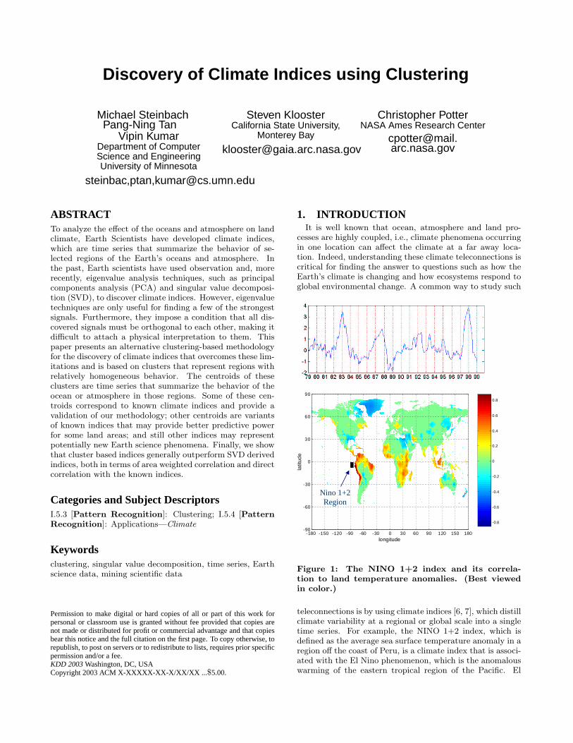
Figure 1: The NINO 1+2 index and its correla-tion to land temperature anomalies. (Best viewedin color.)

teleconnections is by using climate indices [6, 7], which distillclimate variability at a regional or global scale into a singletime series. For example, the NINO 1+2 index, which isdefined as the average sea surface temperature anomaly in aregion off the coast of Peru, is a climate index that is associ-ated with the El Nino phenomenon, which is the anomalouswarming of the eastern tropical region of the Pacific. El

Nino has been linked to climate anomalies in many partsof the world such as droughts in Australia and heavy rain-fall along the eastern coast of South America [18]. Figure1 shows the correlation between the NINO 1+2 index andland temperature anomalies, which are deviations from themean. Observe that this index is highly correlated to theland temperature anomalies on the western coast of SouthAmerica, which is not surprising given the proximity of thisregion to the ocean region defining the index. However, fewoutside the field of Earth Science would expect that NINO1+2 is also highly correlated to land regions that are faraway from the eastern coast of South America, e.g., Africaand South-East Asia.

Most commonly used climate indices are based on sea levelpressure (SLP) and sea surface temperature (SST) in oceanregions. These indices can ease the discovery of relation-ships of SST and SLP to land temperature and precipita-tion. These variables in turn, impact plant growth, and aretherefore important for understanding the global carbon cy-cle and the ecological dynamics of the Earth.

Because of this, Earth Scientists have devoted a consid-erable amount of time to developing/discovering climate in-dices, such as NINO 1+2 and the other indices describedin Table 1. One of the approaches used to discover cli-mate indices has been the direct observation of climate phe-nomenon. For instance, the El Nino phenomenon was firstnoticed by Peruvian fishermen centuries ago. The fishermenobserved that in some years the warm southward current,which appeared around Christmas, would persist for an un-usually long time—a year or so—with a disastrous impacton fishing. In the early 20th century, while studying thetrade winds and Indian monsoon, scientists noticed largescale changes in pressure in the equatorial Pacific regionwhich they referred to as the ‘Southern Oscillation.’ Scien-tists developed a climate index called the Southern Oscilla-tion Index (SOI) to capture this pressure phenomenon. Inthe mid and late 60’s, the Southern Oscillation was conclu-sively tied to El Nino, and their impact on global climatewas recognized. Needless to say, finding climate indices inthis fashion is a very slow and tedious process.

More recently, motivated by the massive amounts of newdata being produced by satellite observations, Earth Scien-tists have been using eigenvalue analysis techniques, such asprincipal components analysis (PCA) and singular value de-composition (SVD), to discover climate indices [16]. Whileeigenvalue techniques do provide a way to quickly and auto-matically detect patterns in large amounts of data, they alsohave the following limitations: (i) all discovered signals mustbe orthogonal to each other, making it difficult to attach aphysical interpretation to them, and (ii) weaker signals maybe masked by stronger signals. These points are discussedin more detail in Section 3.

This paper presents an alternative clustering-based method-ology for the discovery of climate indices that overcomesthese limitations. The use of clustering is driven by the in-tuition that a climate phenomenon is expected to involve asignificant region of the ocean or atmosphere, and that weexpect that such a phenomenon will be ‘stronger’ if it in-volves a region where the behavior is relatively uniform overthe entire area. SNN clustering [2, 3, 4] has been shown tofind such homogeneous clusters. Each of these clusters canbe characterized by a centroid, i.e., the mean of all the timeseries describing the ocean points in the cluster, and thus,

these centroids represent potential climate indices. This ap-proach offers a number of benefits: (i) discovered signalsdo not need to be orthogonal to each other, (ii) signals aremore easily interpreted, (iii) weaker signals are more readilydetected, and (iv) it provides an efficient way to determinethe influence of a large set of points, e.g, all ocean points,on another large set of points, e.g., all land points.

The results of applying our methodology to discover clus-ter indices are encouraging. Some of the cluster centroids,i.e., candidate indices, that we found are very highly corre-lated to known indices. This represents a rediscovery of well-known indices and serves to validate our approach. In fact,we are able to rediscover most of the known major climateindices using our approach. In addition, some of the clustercentroids that have a high correlation to well-known indicesmay represent variants to well-known indices in that, whilethey may represent the same phenomena, they may be po-tentially better predictors of land behavior for some regionsof the land. Finally, cluster centroids that have medium orlow correlation with known indices may represent potentiallynew Earth science phenomena.

This paper is organized as follows: Section 2 provides aquick introduction to Earth Science data and climate in-dices, while Section 3 provides a more detailed look at howeigenvalue techniques are used to discover climate indicesand the limitations of this approach. Section 4 describesour methodology and Sections 5 presents the results of ap-plying this methodology to find climate indices that have astrong connection to land temperature. Section 6 summa-rizes our work and indicates future directions. Our prelimi-nary results on this topic have appeared in several workshoppapers [17, 14, 15, 13].

2. EARTH SCIENCE DATA AND CLIMATEINDICES

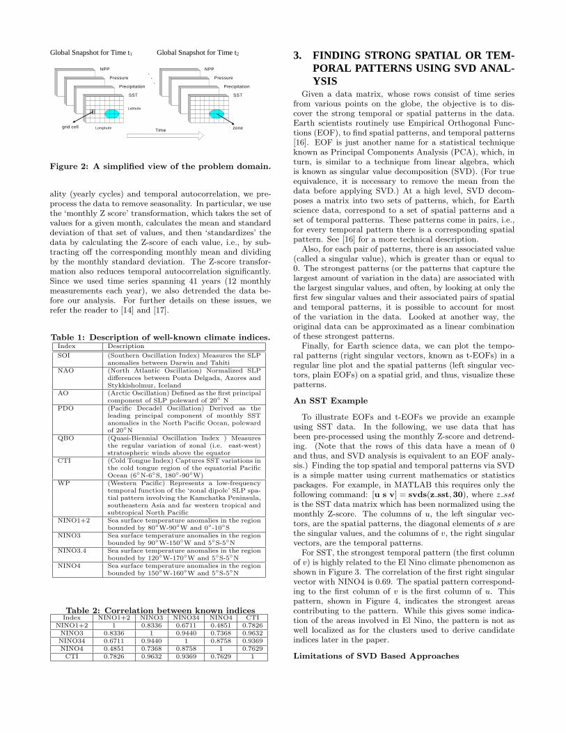
The Earth science data for our analysis consists of globalsnapshots of measurement values for a number of variables(e.g., temperature, pressure and precipitation) collected forall land and sea surfaces (see Figure 2). These variable val-ues are either observations from different sensors, e.g., pre-cipitation, Sea Level Pressure (SLP), sea surface tempera-ture (SST), or the result of model predictions, e.g., NPP(Net Primary Production or plant growth) from the CASAmodel [10], and are typically available at monthly intervalsthat span a range of 10 to 50 years. For the analysis pre-sented here, we focus on attributes measured at points (gridcells) on latitude-longitude spherical grids of different reso-lutions, e.g., land temperature, which is available at a reso-lution of 0.5◦×0.5◦, and SST, which is available for a 1◦×1◦

grid, and SLP, which is available for a 2.5◦ × 2.5◦ grid.Most of the well-known climate indices [6, 7] based upon

SST and SLP are shown in Table 1. Many of the indices rep-resent the El Nino phenomenon and are highly correlated,as shown in Table 2. Figure 1 shows the time series for theNINO 1+2 index. The peaks correspond to El Nino events.

The spatial and temporal nature of Earth Science posesa number of challenges. For instance, Earth Science timeseries data is noisy, has cycles of varying lengths and reg-ularity, and can contain long term trends. In addition,such data displays spatial and temporal autocorrelation, i.e.,measured values that are close in time and space tend to behighly correlated, or similar. To handle the issues of season-

Global Snapshot for Time t1 Global Snapshot for Time t2

SST

Precipitation

NPP

Pressure

SST

Precipitation

NPP

Pressure

Longitude

Latitude

Timegrid cell zone

...

Figure 2: A simplified view of the problem domain.

ality (yearly cycles) and temporal autocorrelation, we pre-process the data to remove seasonality. In particular, we usethe ‘monthly Z score’ transformation, which takes the set ofvalues for a given month, calculates the mean and standarddeviation of that set of values, and then ‘standardizes’ thedata by calculating the Z-score of each value, i.e., by sub-tracting off the corresponding monthly mean and dividingby the monthly standard deviation. The Z-score transfor-mation also reduces temporal autocorrelation significantly.Since we used time series spanning 41 years (12 monthlymeasurements each year), we also detrended the data be-fore our analysis. For further details on these issues, werefer the reader to [14] and [17].

Table 1: Description of well-known climate indices.Index Description

SOI (Southern Oscillation Index) Measures the SLPanomalies between Darwin and Tahiti

NAO (North Atlantic Oscillation) Normalized SLPdifferences between Ponta Delgada, Azores andStykkisholmur, Iceland

AO (Arctic Oscillation) Defined as the first principalcomponent of SLP poleward of 20◦ N

PDO (Pacific Decadel Oscillation) Derived as theleading principal component of monthly SSTanomalies in the North Pacific Ocean, polewardof 20◦N

QBO (Quasi-Biennial Oscillation Index ) Measuresthe regular variation of zonal (i.e. east-west)stratospheric winds above the equator

CTI (Cold Tongue Index) Captures SST variations inthe cold tongue region of the equatorial PacificOcean (6◦N-6◦S, 180◦-90◦W)

WP (Western Pacific) Represents a low-frequencytemporal function of the ‘zonal dipole’ SLP spa-tial pattern involving the Kamchatka Peninsula,southeastern Asia and far western tropical andsubtropical North Pacific

NINO1+2 Sea surface temperature anomalies in the regionbounded by 80◦W-90◦W and 0◦-10◦S

NINO3 Sea surface temperature anomalies in the regionbounded by 90◦W-150◦W and 5◦S-5◦N

NINO3.4 Sea surface temperature anomalies in the regionbounded by 120◦W-170◦W and 5◦S-5◦N

NINO4 Sea surface temperature anomalies in the regionbounded by 150◦W-160◦W and 5◦S-5◦N

Table 2: Correlation between known indicesIndex NINO1+2 NINO3 NINO34 NINO4 CTI

NINO1+2 1 0.8336 0.6711 0.4851 0.7826NINO3 0.8336 1 0.9440 0.7368 0.9632NINO34 0.6711 0.9440 1 0.8758 0.9369NINO4 0.4851 0.7368 0.8758 1 0.7629CTI 0.7826 0.9632 0.9369 0.7629 1

3. FINDING STRONG SPATIAL OR TEM-PORAL PATTERNS USING SVD ANAL-YSIS

Given a data matrix, whose rows consist of time seriesfrom various points on the globe, the objective is to dis-cover the strong temporal or spatial patterns in the data.Earth scientists routinely use Empirical Orthogonal Func-tions (EOF), to find spatial patterns, and temporal patterns[16]. EOF is just another name for a statistical techniqueknown as Principal Components Analysis (PCA), which, inturn, is similar to a technique from linear algebra, whichis known as singular value decomposition (SVD). (For trueequivalence, it is necessary to remove the mean from thedata before applying SVD.) At a high level, SVD decom-poses a matrix into two sets of patterns, which, for Earthscience data, correspond to a set of spatial patterns and aset of temporal patterns. These patterns come in pairs, i.e.,for every temporal pattern there is a corresponding spatialpattern. See [16] for a more technical description.

Also, for each pair of patterns, there is an associated value(called a singular value), which is greater than or equal to0. The strongest patterns (or the patterns that capture thelargest amount of variation in the data) are associated withthe largest singular values, and often, by looking at only thefirst few singular values and their associated pairs of spatialand temporal patterns, it is possible to account for mostof the variation in the data. Looked at another way, theoriginal data can be approximated as a linear combinationof these strongest patterns.

Finally, for Earth science data, we can plot the tempo-ral patterns (right singular vectors, known as t-EOFs) in aregular line plot and the spatial patterns (left singular vec-tors, plain EOFs) on a spatial grid, and thus, visualize thesepatterns.

An SST Example

To illustrate EOFs and t-EOFs we provide an exampleusing SST data. In the following, we use data that hasbeen pre-processed using the monthly Z-score and detrend-ing. (Note that the rows of this data have a mean of 0and thus, and SVD analysis is equivalent to an EOF analy-sis.) Finding the top spatial and temporal patterns via SVDis a simple matter using current mathematics or statisticspackages. For example, in MATLAB this requires only thefollowing command: [u s v] = svds(z sst,30), where z sstis the SST data matrix which has been normalized using themonthly Z-score. The columns of u, the left singular vec-tors, are the spatial patterns, the diagonal elements of s arethe singular values, and the columns of v, the right singularvectors, are the temporal patterns.

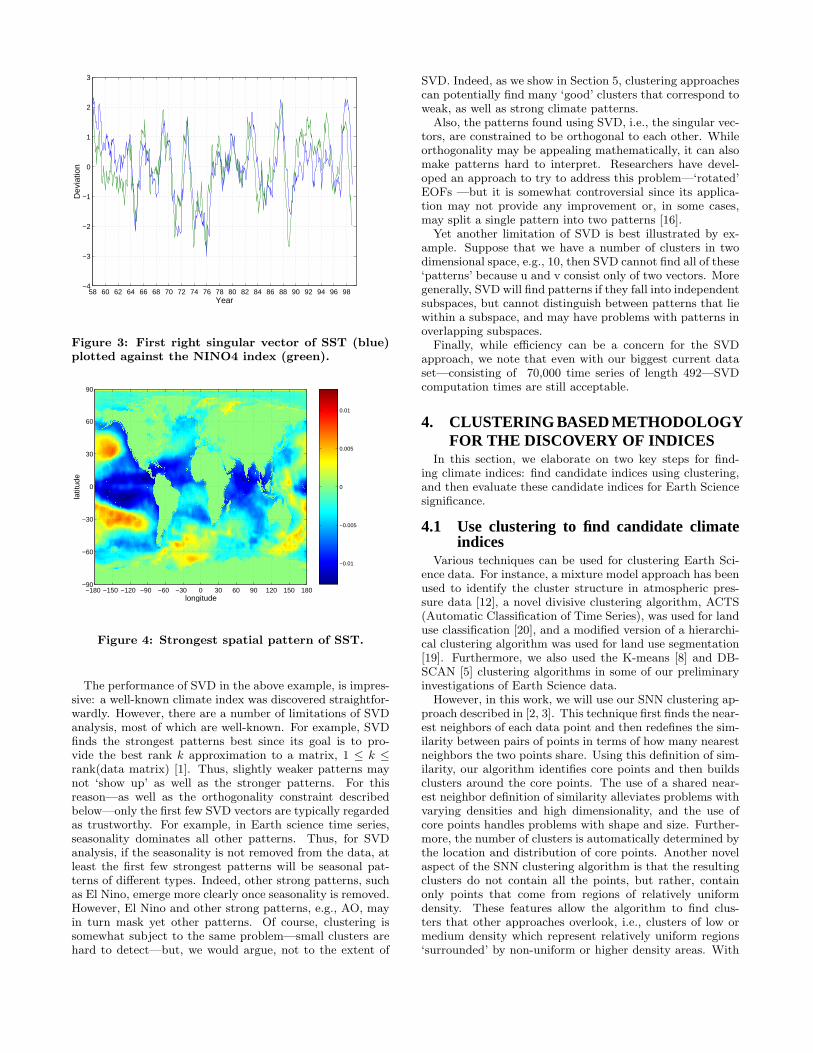
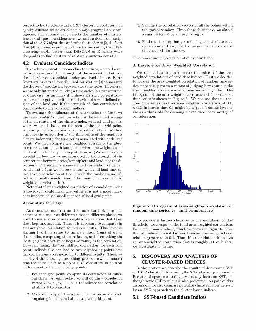
For SST, the strongest temporal pattern (the first columnof v) is highly related to the El Nino climate phenomenon asshown in Figure 3. The correlation of the first right singularvector with NINO4 is 0.69. The spatial pattern correspond-ing to the first column of v is the first column of u. Thispattern, shown in Figure 4, indicates the strongest areascontributing to the pattern. While this gives some indica-tion of the areas involved in El Nino, the pattern is not aswell localized as for the clusters used to derive candidateindices later in the paper.

Limitations of SVD Based Approaches

58 60 62 64 66 68 70 72 74 76 78 80 82 84 86 88 90 92 94 96 98−4

−3

−2

−1

0

1

2

3

Year

Dev

iatio

n

Figure 3: First right singular vector of SST (blue)plotted against the NINO4 index (green).

−0.01

−0.005

0

0.005

0.01

longitude

latit

ude

−180 −150 −120 −90 −60 −30 0 30 60 90 120 150 180

90

60

30

0

−30

−60

−90

Figure 4: Strongest spatial pattern of SST.

The performance of SVD in the above example, is impres-sive: a well-known climate index was discovered straightfor-wardly. However, there are a number of limitations of SVDanalysis, most of which are well-known. For example, SVDfinds the strongest patterns best since its goal is to pro-vide the best rank k approximation to a matrix, 1 ≤ k ≤rank(data matrix) [1]. Thus, slightly weaker patterns maynot ‘show up’ as well as the stronger patterns. For thisreason—as well as the orthogonality constraint describedbelow—only the first few SVD vectors are typically regardedas trustworthy. For example, in Earth science time series,seasonality dominates all other patterns. Thus, for SVDanalysis, if the seasonality is not removed from the data, atleast the first few strongest patterns will be seasonal pat-terns of different types. Indeed, other strong patterns, suchas El Nino, emerge more clearly once seasonality is removed.However, El Nino and other strong patterns, e.g., AO, mayin turn mask yet other patterns. Of course, clustering issomewhat subject to the same problem—small clusters arehard to detect—but, we would argue, not to the extent of

SVD. Indeed, as we show in Section 5, clustering approachescan potentially find many ‘good’ clusters that correspond toweak, as well as strong climate patterns.

Also, the patterns found using SVD, i.e., the singular vec-tors, are constrained to be orthogonal to each other. Whileorthogonality may be appealing mathematically, it can alsomake patterns hard to interpret. Researchers have devel-oped an approach to try to address this problem—‘rotated’EOFs —but it is somewhat controversial since its applica-tion may not provide any improvement or, in some cases,may split a single pattern into two patterns [16].

Yet another limitation of SVD is best illustrated by ex-ample. Suppose that we have a number of clusters in twodimensional space, e.g., 10, then SVD cannot find all of these‘patterns’ because u and v consist only of two vectors. Moregenerally, SVD will find patterns if they fall into independentsubspaces, but cannot distinguish between patterns that liewithin a subspace, and may have problems with patterns inoverlapping subspaces.

Finally, while efficiency can be a concern for the SVDapproach, we note that even with our biggest current dataset—consisting of 70,000 time series of length 492—SVDcomputation times are still acceptable.

4. CLUSTERING BASED METHODOLOGYFOR THE DISCOVERY OF INDICES

In this section, we elaborate on two key steps for find-ing climate indices: find candidate indices using clustering,and then evaluate these candidate indices for Earth Sciencesignificance.

4.1 Use clustering to find candidate climateindices

Various techniques can be used for clustering Earth Sci-ence data. For instance, a mixture model approach has beenused to identify the cluster structure in atmospheric pres-sure data [12], a novel divisive clustering algorithm, ACTS(Automatic Classification of Time Series), was used for landuse classification [20], and a modified version of a hierarchi-cal clustering algorithm was used for land use segmentation[19]. Furthermore, we also used the K-means [8] and DB-SCAN [5] clustering algorithms in some of our preliminaryinvestigations of Earth Science data.

However, in this work, we will use our SNN clustering ap-proach described in [2, 3]. This technique first finds the near-est neighbors of each data point and then redefines the sim-ilarity between pairs of points in terms of how many nearestneighbors the two points share. Using this definition of sim-ilarity, our algorithm identifies core points and then buildsclusters around the core points. The use of a shared near-est neighbor definition of similarity alleviates problems withvarying densities and high dimensionality, and the use ofcore points handles problems with shape and size. Further-more, the number of clusters is automatically determined bythe location and distribution of core points. Another novelaspect of the SNN clustering algorithm is that the resultingclusters do not contain all the points, but rather, containonly points that come from regions of relatively uniformdensity. These features allow the algorithm to find clus-ters that other approaches overlook, i.e., clusters of low ormedium density which represent relatively uniform regions‘surrounded’ by non-uniform or higher density areas. With

respect to Earth Science data, SNN clustering produces highquality clusters, which are almost always geographically con-tiguous, and automatically selects the number of clusters.Because of space considerations, we omit a detailed descrip-tion of the SNN algorithm and refer the reader to [2, 4]. Notethat [4] contains experimental results indicating that SNNclustering works better than DBSCAN or K-means whenthe goal is to find clusters of relatively uniform densities.

4.2 Evaluate Candidate IndicesTo evaluate potential ocean climate indices, we need a nu-

merical measure of the strength of the association betweenthe behavior of a candidate index and land climate. EarthScientists have traditionally used correlation [9] to measurethe degree of association between two time series. In general,we are only interested in using a time series (cluster centroid,or otherwise) as an index if it shows a strong correlation—positive or negative—with the behavior of a well-defined re-gion of the land and if the strength of that correlation iscomparable to that of known indices.

To evaluate the influence of climate indices on land, weuse area-weighted correlation, which is the weighted averageof the correlation of the climate index with all land points,where weight is based on the area of the land grid point.Area-weighted correlation is computed as follows. We firstcompute the correlation of the time series of the candidateclimate index with the time series associated with each landpoint. We then compute the weighted average of the abso-lute correlations of each land point, where the weight associ-ated with each land point is just its area. (We use absolutecorrelation because we are interested in the strength of theconnections between ocean/atmosphere and land, not the di-rection.) The resulting area-weighted correlation value canbe at most 1 (this would be the case where all land time se-ries have a correlation of 1 or -1 with the candidate index),but is normally much lower. The minimum value of areaweighted correlation is 0.

Note that if area weighted correlation of a candidate indexis too low, it could mean that either it is not a good index,or it impacts only a small number of land grid points.

Accounting for Lags

As mentioned earlier, since the same Earth Science phe-nomenon can occur at different times in different places, wewant to use a form of area weighted correlation that takesthese lags into account. Thus, it is necessary to compute thearea-weighted correlation for various shifts. This involvesshifting two time series to simulate leads (lags) of up tosix months, computing the correlation, and then taking the‘best’ (highest positive or negative value) as the correlation.However, taking the ‘best shifted correlation’ for each landpoint, individually, can lead to two neighboring points hav-ing correlations corresponding to different shifts. Thus, weemployed the following ‘smoothing’ procedure which ensuresthat the ‘best’ shift at a point is as consistent as possiblewith respect to its neighboring points.

1. For each grid point, compute its correlation at differ-ent shifts. At each point, we will obtain a correlationvector < c0, c1, c2, · · · , c6 > to indicate the correlationat shifts 0 to 6 months.

2. Construct a spatial window, which is an m × n rect-angular grid, centered about a given grid point.

3. Sum up the correlation vectors of all the points withinthe spatial window. Thus, for each window, we obtaina sum vector: < σ0, σ1, σ2, · · · , σ6 >.

4. Find the time lag that gives the highest absolute totalcorrelation and assign it to the grid point located atthe center of the window.

This procedure is used in all of our evaluations.

A Baseline for Area Weighted Correlation

We need a baseline to compare the values of the areaweighted correlations of candidate indices. First we decidedto look at the area weighted correlation of random time se-ries since this gives us a means of judging how spurious thearea weighted correlation of a time series might be. Thehistogram of the area weighted correlation of 1000 randomtime series is shown in Figure 5. We can see that no ran-dom time series have an area weighted correlation of 0.1,which indicates that 0.l might be a good baseline level touse as a threshold for deeming a candidate index worthy ofconsideration.

0.06 0.065 0.07 0.075 0.08 0.085 0.09 0.095 0.10

5

10

15

20

25

30

35

Area Weighted Correlation

Cou

nt

Figure 5: Histogram of area-weighted correlation ofrandom time series vs. land temperature.

To provide a further check as to the usefulness of thisthreshold, we computed the total area-weighted correlationsfor 11 well-known indices, which are shown in Figure 6. Notethat all indices, except for one, have an area weighted cor-relation greater than 0.1. Thus, if a candidate index showsan area-weighted correlation that is roughly 0.1 or higher,we investigate it further.

5. DISCOVERY AND ANALYSIS OFCLUSTER-BASED INDICES

In this section we describe the results of discovering SSTand SLP climate indices using the SNN clustering approach.Because of space constraints, we mostly focus on SST, al-though some SLP results are also presented. As part of thisdiscussion, we also compare potential climate indices derivedby an SVD approach to the cluster-based indices.

5.1 SST-based Candidate Indices

SOI NAO AO PDO QBO CTI WP NINO12 NINO3 NINO34 NINO40

0.05

0.1

0.15

0.2

Figure 6: Area weighted correlation of well-knownindices.

Figure 7: 107 SST clusters.

We applied SNN clustering on the SST data over the timeperiod from 1958 to 1998. There are 107 clusters found bySNN, as shown in Figure 7. Note that many grid pointsfrom the ocean do not belong to any clusters (these are thepoints belonging to the white background), as these pointscome from regions that are not relatively uniform and ho-mogeneous. Since we are mainly interested in finding strongcandidate indices, we first eliminate all clusters with poorarea-weighted correlation, i.e., below the specified baselineof 0.1. The cluster centroids of the remaining clusters arepotential candidate indices.

For further evaluation of the candidate indices, we dividedthe cluster centroids into 4 groups, G0, G1, G2, and G3, de-pending on the correlation of the cluster centroids to knownindices. Cluster centroids (G0) that are very highly corre-lated to known indices represent a rediscovery of well-knownindices and serve to validate our approach. Cluster centroids(G1) that have a high correlation to well-known indices rep-

resent variants of existing indices, but can be useful alterna-tives if they are better predictors of land behavior, at leastfor some regions of the land. Finally, cluster centroids (G2and G3) with medium to low correlation may represent po-tentially new Earth science phenomena. These four groupsof clusters are shown in Figures 8-11.

Clusters 58 59 67 75 78 94

58 59

6775 78 94

-180 -140 -100 -60 -20 20 60 100 140 180

90

70

50

30

10

-10

-30

-50

-70

-90

Figure 8: G0: Clusters with correlation to knownindices ≥ 0.8.

Clusters 11 17 20 24 28 29 31 36 37 57 80 81 83 92 97

1117

20

24

28

29

31

36

3757

80

8183

92

97

-180 -140 -100 -60 -20 20 60 100 140 180

90

70

50

30

10

-10

-30

-50

-70

-90

Figure 9: G1: Clusters with correlation to knownindices between 0.4 and 0.8.

Candidate Indices Similar to Known Indices

Figure 8 shows clusters that reproduce some well-knownclimate indices. In particular, we were able to replicate thefour El Nino SST-based indices: cluster 94 corresponds toNINO 1+2, 67 to NINO 3, 78 to NINO 3.4, and 75 to NINO4. The correlations of these clusters to their correspondingindices are higher than 0.9, as shown in the second and thirdcolumns of Table 3. In addition, cluster 67 is highly corre-lated to the CTI index, which is defined over a wider areain the same region. Clusters 58 and 59 are very similar tothe other El Nino indices, and correlate most strongly withNINO 3 and NINO 4, respectively. But their correlations to

Clusters 13 19 27 62 71 100 104

13

19

27

62

71 100

104

-180 -140 -100 -60 -20 20 60 100 140 180

90

70

50

30

10

-10

-30

-50

-70

-90

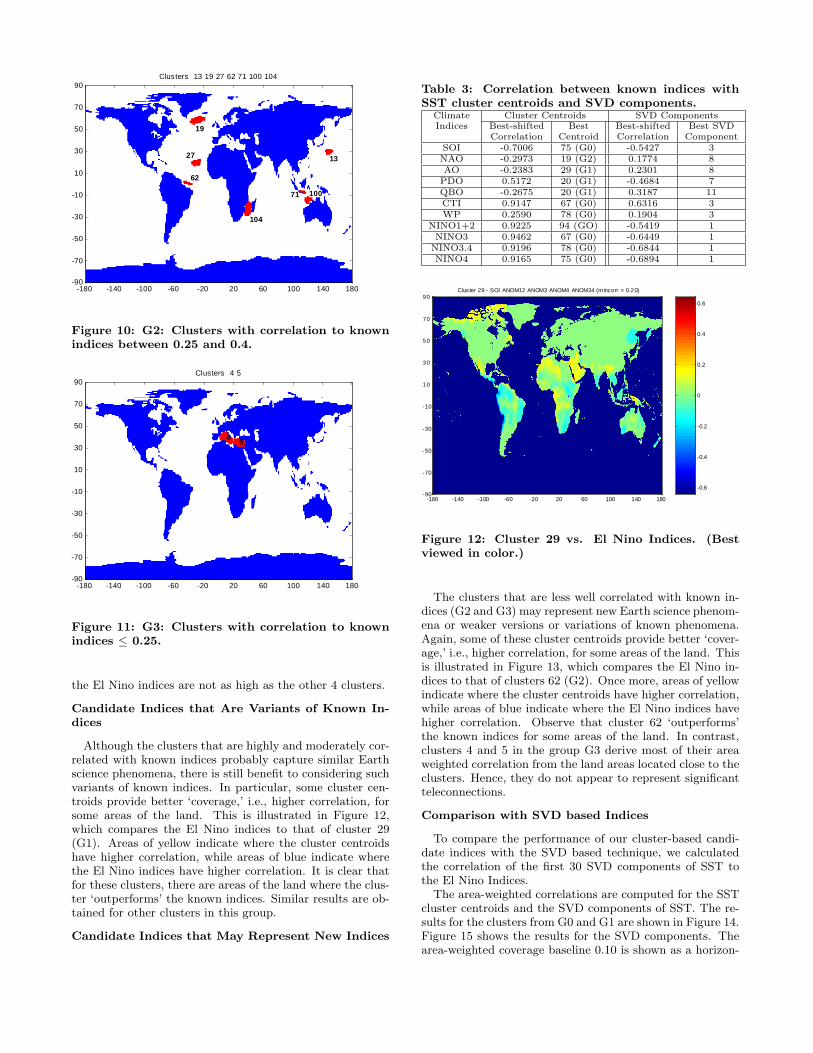
Figure 10: G2: Clusters with correlation to knownindices between 0.25 and 0.4.

Clusters 4 5

4 5

-180 -140 -100 -60 -20 20 60 100 140 180

90

70

50

30

10

-10

-30

-50

-70

-90

Figure 11: G3: Clusters with correlation to knownindices ≤ 0.25.

the El Nino indices are not as high as the other 4 clusters.

Candidate Indices that Are Variants of Known In-dices

Although the clusters that are highly and moderately cor-related with known indices probably capture similar Earthscience phenomena, there is still benefit to considering suchvariants of known indices. In particular, some cluster cen-troids provide better ‘coverage,’ i.e., higher correlation, forsome areas of the land. This is illustrated in Figure 12,which compares the El Nino indices to that of cluster 29(G1). Areas of yellow indicate where the cluster centroidshave higher correlation, while areas of blue indicate wherethe El Nino indices have higher correlation. It is clear thatfor these clusters, there are areas of the land where the clus-ter ‘outperforms’ the known indices. Similar results are ob-tained for other clusters in this group.

Candidate Indices that May Represent New Indices

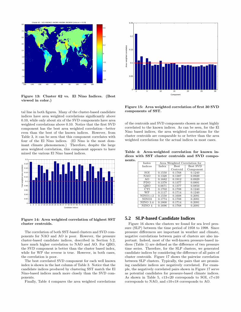
Table 3: Correlation between known indices withSST cluster centroids and SVD components.

Climate Cluster Centroids SVD ComponentsIndices Best-shifted Best Best-shifted Best SVD

Correlation Centroid Correlation ComponentSOI -0.7006 75 (G0) -0.5427 3NAO -0.2973 19 (G2) 0.1774 8AO -0.2383 29 (G1) 0.2301 8

PDO 0.5172 20 (G1) -0.4684 7QBO -0.2675 20 (G1) 0.3187 11CTI 0.9147 67 (G0) 0.6316 3WP 0.2590 78 (G0) 0.1904 3

NINO1+2 0.9225 94 (GO) -0.5419 1NINO3 0.9462 67 (G0) -0.6449 1

NINO3.4 0.9196 78 (G0) -0.6844 1NINO4 0.9165 75 (G0) -0.6894 1

-0.6

-0.4

-0.2

0

0.2

0.4

0.6

Cluster 29 - SOI ANOM12 ANOM3 ANOM4 ANOM34 (mincorr = 0.20)

-180 -140 -100 -60 -20 20 60 100 140 180

90

70

50

30

10

-10

-30

-50

-70

-90

Figure 12: Cluster 29 vs. El Nino Indices. (Bestviewed in color.)

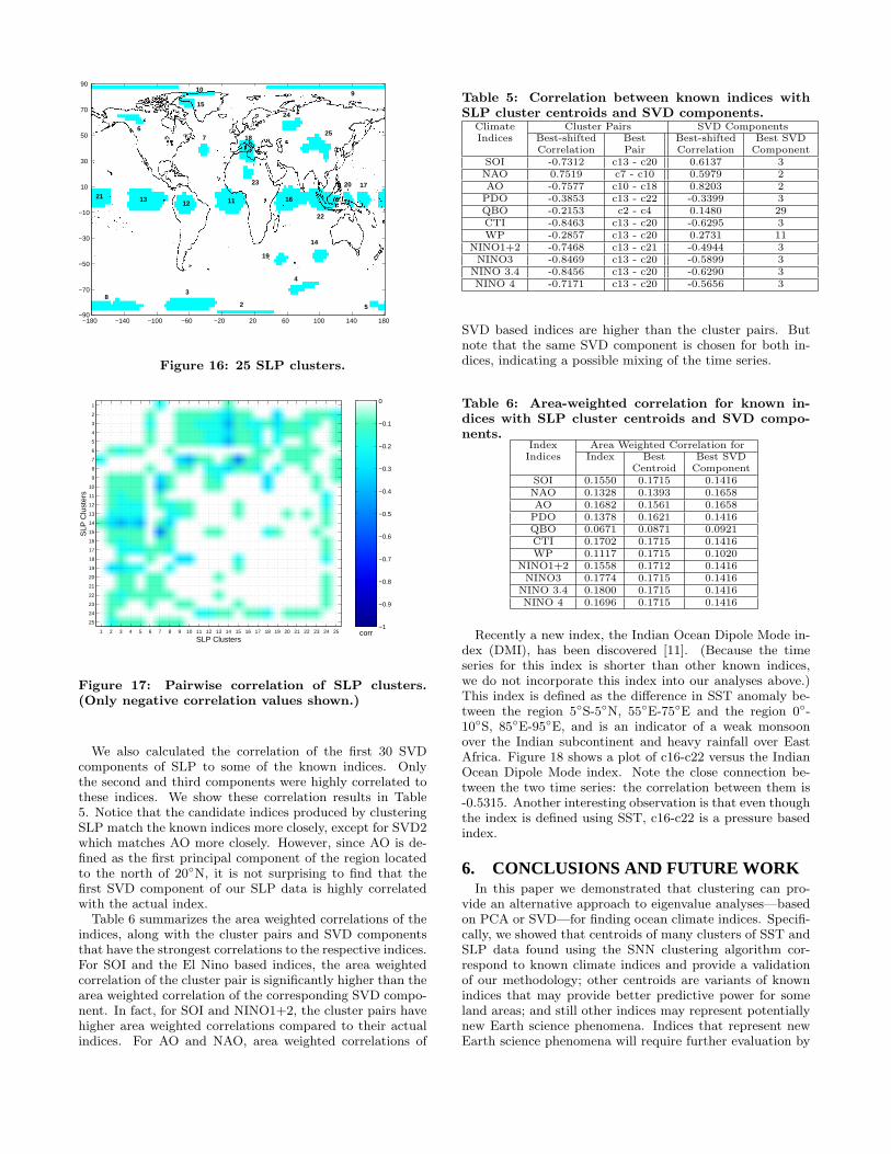
The clusters that are less well correlated with known in-dices (G2 and G3) may represent new Earth science phenom-ena or weaker versions or variations of known phenomena.Again, some of these cluster centroids provide better ‘cover-age,’ i.e., higher correlation, for some areas of the land. Thisis illustrated in Figure 13, which compares the El Nino in-dices to that of clusters 62 (G2). Once more, areas of yellowindicate where the cluster centroids have higher correlation,while areas of blue indicate where the El Nino indices havehigher correlation. Observe that cluster 62 ‘outperforms’the known indices for some areas of the land. In contrast,clusters 4 and 5 in the group G3 derive most of their areaweighted correlation from the land areas located close to theclusters. Hence, they do not appear to represent significantteleconnections.

Comparison with SVD based Indices

To compare the performance of our cluster-based candi-date indices with the SVD based technique, we calculatedthe correlation of the first 30 SVD components of SST tothe El Nino Indices.

The area-weighted correlations are computed for the SSTcluster centroids and the SVD components of SST. The re-sults for the clusters from G0 and G1 are shown in Figure 14.Figure 15 shows the results for the SVD components. Thearea-weighted coverage baseline 0.10 is shown as a horizon-

-0.6

-0.4

-0.2

0

0.2

0.4

0.6

Cluster 62 - SOI ANOM12 ANOM3 ANOM4 ANOM34 (mincorr = 0.20)

-180 -140 -100 -60 -20 20 60 100 140 180

90

70

50

30

10

-10

-30

-50

-70

-90

Figure 13: Cluster 62 vs. El Nino Indices. (Bestviewed in color.)

tal line in both figures. Many of the cluster-based candidateindices have area weighted correlations significantly above0.10, while only about six of the SVD components have areaweighted correlations above 0.10. Notice that the first SVDcomponent has the best area weighted correlation—bettereven than the best of the known indices. However, fromTable 3, it can be seen that this component correlates withfour of the El Nino indices. (El Nino is the most dom-inant climate phenomenon.) Therefore, despite the largearea weighted correlation, this component appears to havemixed the various El Nino based indices.

1 8 9 11 17 20 24 25 28 29 31 36 37 57 58 59 67 68 75 78 79 80 81 83 87 92 94 95 96 97 990

0.02

0.04

0.06

0.08

0.1

0.12

0.14

0.16

0.18

0.2

Candidate indices

Tot

al w

eigh

ted

area

cor

rela

tion

Figure 14: Area weighted correlation of highest SSTcluster centroids.

The correlation of both SST-based clusters and SVD com-ponents for NAO and AO is poor. However, the pressurecluster-based candidate indices, described in Section 5.2,have much higher correlation to NAO and AO. For QBO,the SVD component is better than the cluster based index,while for WP the reverse is true. However, in both cases,the correlation is poor.

The best correlated SVD component for each well knownindex is shown in the last column of Table 3. Notice that thecandidate indices produced by clustering SST match the ElNino-based indices much more closely than the SVD com-ponents.

Finally, Table 4 compares the area weighted correlations

1 5 10 15 20 25 300

0.05

0.1

0.15

0.2

0.25

Component

Are

a−w

eigh

ted

corr

elat

ion

Figure 15: Area weighted correlation of first 30 SVDcomponents of SST.

of the centroids and SVD components chosen as most highlycorrelated to the known indices. As can be seen, for the ElNino based indices, the area weighted correlations for thecluster centroids are comparable to or better than the areaweighted correlations for the actual indices in most cases.

Table 4: Area-weighted correlation for known in-dices with SST cluster centroids and SVD compo-nents.

Index Area Weighted Correlation forIndices Index Best Best SVD

Centroid ComponentSOI 0.1550 0.1768 0.1240NAO 0.1328 0.1387 0.0929AO 0.1682 0.1912 0.0929

PDO 0.1378 0.1377 0.0891QBO 0.0671 0.1377 0.0850CTI 0.1702 0.1708 0.1240WP 0.1117 0.1714 0.1240

NINO1+2 0.1558 0.1608 0.2091NINO3 0.1774 0.1708 0.2091

NINO 3.4 0.1800 0.1714 0.2091NINO 4 0.1696 0.1768 0.2091

5.2 SLP-based Candidate IndicesFigure 16 shows the clusters we found for sea level pres-

sure (SLP) between the time period of 1958 to 1998. Sincepressure differences are important in weather and climate,negative correlations between pairs of clusters are also im-portant. Indeed, most of the well-known pressure-based in-dices (Table 1) are defined as the difference of two pressuretime series. Therefore, for the SLP clusters, we generatedcandidate indices by considering the difference of all pairs ofcluster centroids. Figure 17 shows the pairwise correlationbetween SLP clusters. Typically, the pairs that are promis-ing candidate indices are negatively correlated. For exam-ple, the negatively correlated pairs shown in Figure 17 serveas potential candidates for pressure-based climate indices.As shown in Table 5, c13-c20 corresponds to SOI, c7-c10corresponds to NAO, and c10-c18 corresponds to AO.

2

3

4

5

67

8

910

111213

14

15

16

17

18

19

20

21

22

23

24

25

−180 −140 −100 −60 −20 20 60 100 140 180

90

70

50

30

10

−10

−30

−50

−70

−90

Figure 16: 25 SLP clusters.

SLP Clusters

SLP

Clu

ster

s

1 2 3 4 5 6 7 8 9 10 11 12 13 14 15 16 17 18 19 20 21 22 23 24 25

1

2

3

4

5

6

7

8

9

10

11

12

13

14

15

16

17

18

19

20

21

22

23

24

25

corr−1

−0.9

−0.8

−0.7

−0.6

−0.5

−0.4

−0.3

−0.2

−0.1

0

Figure 17: Pairwise correlation of SLP clusters.(Only negative correlation values shown.)

We also calculated the correlation of the first 30 SVDcomponents of SLP to some of the known indices. Onlythe second and third components were highly correlated tothese indices. We show these correlation results in Table5. Notice that the candidate indices produced by clusteringSLP match the known indices more closely, except for SVD2which matches AO more closely. However, since AO is de-fined as the first principal component of the region locatedto the north of 20◦N, it is not surprising to find that thefirst SVD component of our SLP data is highly correlatedwith the actual index.

Table 6 summarizes the area weighted correlations of theindices, along with the cluster pairs and SVD componentsthat have the strongest correlations to the respective indices.For SOI and the El Nino based indices, the area weightedcorrelation of the cluster pair is significantly higher than thearea weighted correlation of the corresponding SVD compo-nent. In fact, for SOI and NINO1+2, the cluster pairs havehigher area weighted correlations compared to their actualindices. For AO and NAO, area weighted correlations of

Table 5: Correlation between known indices withSLP cluster centroids and SVD components.

Climate Cluster Pairs SVD ComponentsIndices Best-shifted Best Best-shifted Best SVD

Correlation Pair Correlation ComponentSOI -0.7312 c13 - c20 0.6137 3NAO 0.7519 c7 - c10 0.5979 2AO -0.7577 c10 - c18 0.8203 2

PDO -0.3853 c13 - c22 -0.3399 3QBO -0.2153 c2 - c4 0.1480 29CTI -0.8463 c13 - c20 -0.6295 3WP -0.2857 c13 - c20 0.2731 11

NINO1+2 -0.7468 c13 - c21 -0.4944 3NINO3 -0.8469 c13 - c20 -0.5899 3

NINO 3.4 -0.8456 c13 - c20 -0.6290 3NINO 4 -0.7171 c13 - c20 -0.5656 3

SVD based indices are higher than the cluster pairs. Butnote that the same SVD component is chosen for both in-dices, indicating a possible mixing of the time series.

Table 6: Area-weighted correlation for known in-dices with SLP cluster centroids and SVD compo-nents.

Index Area Weighted Correlation forIndices Index Best Best SVD

Centroid ComponentSOI 0.1550 0.1715 0.1416NAO 0.1328 0.1393 0.1658AO 0.1682 0.1561 0.1658

PDO 0.1378 0.1621 0.1416QBO 0.0671 0.0871 0.0921CTI 0.1702 0.1715 0.1416WP 0.1117 0.1715 0.1020

NINO1+2 0.1558 0.1712 0.1416NINO3 0.1774 0.1715 0.1416

NINO 3.4 0.1800 0.1715 0.1416NINO 4 0.1696 0.1715 0.1416

Recently a new index, the Indian Ocean Dipole Mode in-dex (DMI), has been discovered [11]. (Because the timeseries for this index is shorter than other known indices,we do not incorporate this index into our analyses above.)This index is defined as the difference in SST anomaly be-tween the region 5◦S-5◦N, 55◦E-75◦E and the region 0◦-10◦S, 85◦E-95◦E, and is an indicator of a weak monsoonover the Indian subcontinent and heavy rainfall over EastAfrica. Figure 18 shows a plot of c16-c22 versus the IndianOcean Dipole Mode index. Note the close connection be-tween the two time series: the correlation between them is-0.5315. Another interesting observation is that even thoughthe index is defined using SST, c16-c22 is a pressure basedindex.

6. CONCLUSIONS AND FUTURE WORKIn this paper we demonstrated that clustering can pro-

vide an alternative approach to eigenvalue analyses—basedon PCA or SVD—for finding ocean climate indices. Specifi-cally, we showed that centroids of many clusters of SST andSLP data found using the SNN clustering algorithm cor-respond to known climate indices and provide a validationof our methodology; other centroids are variants of knownindices that may provide better predictive power for someland areas; and still other indices may represent potentiallynew Earth science phenomena. Indices that represent newEarth science phenomena will require further evaluation by

82 83 84 85 86 87 88 89 90 91 92 93 94 95 96 97 98−2

−1.5

−1

−0.5

0

0.5

1

1.5

2

2.5

3Cluster 16 − Cluster 22

Figure 18: Plot of c16-c22 versus the Indian OceanDipole Mode index. (Indices smoothed using 12month moving average.

domain specialists. In addition, we compared potential in-dices derived from using SVD to our candidate indices andto well-known indices, showing that, in general, the SVD de-rived indices had lower area weighted correlation than manyof the cluster-derived candidate indices and the well-knownindices. This comparison showed that cluster based indicesgenerally outperform SVD derived indices, both in termsof area weighted correlation and direct correlation with theknown indices.

It should be noted that SVD results were obtained by us-ing the data for the entire ocean (SST), or for SLP, for theentire globe. Earth scientists typically apply SVD analy-sis to a select region. However, it requires a considerableamount of domain knowledge to determine the appropriatearea. Clustering on the other hand, provides a means ofautomatically identifying regions that may be of interest.

In the future, we plan to extend our current work to ad-dress several unresolved issues. Specifically, we want todetermine if there are any climate indices that cannot berepresented using clusters. Also, we have also begun to in-vestigate the effect of eliminating any correlations whosemagnitudes are below a certain threshold. The idea is toeliminate noise and to see if looking only at stronger corre-lations produces better results. Finally, we intend to extendour analyses to other land and ocean variables and to inves-tigate ways of aggregating the data so as to make patternseasier to detect.

7. ACKNOWLEDGMENTSThis work was partially supported by NASA grant # NCC

2 1231, NSF ACI-9982274. and by Army High PerformanceComputing Research Center cooperative agreement numberDAAD19-01-2-0014. The content of this work does not nec-essarily reflect the position or policy of the government andno official endorsement should be inferred. Access to com-puting facilities was provided by the AHPCRC and the Min-nesota Supercomputing Institute.

8. REFERENCES

[1] J. W. Demmel. Applied Numerical Linear Algebra. SIAM,January 1997.

[2] L. Ertoz, M. Steinbach, and V. Kumar. Finding topics incollections of documents: A shared nearest neighborapproach. In Proceedings of Text Mine’01, First SIAMInternational Conference on Data Mining, Chicago, IL,USA, 2001.

[3] L. Ertoz, M. Steinbach, and V. Kumar. A new sharednearest neighbor clustering algorithm and its applications.In Workshop on Clustering High Dimensional Data and itsApplications, SIAM Data Mining 2002, Arlington, VA,USA, 2002.

[4] L. Ertoz, M. Steinbach, and V. Kumar. Finding clusters ofdifferent sizes, shapes, and densities in noisy, highdimensional data. In Proceedings of Second SIAMInternational Conference on Data Mining, San Francisco,CA, USA, 2003, to appear.

[5] M. Ester, H.-P. Kriegel, J. Sander, and X. Xu. Adensity-based algorithm for discovering clusters in largespatial databases with noise. In KDD 1996, pages 226–231,1996.

[6] http://www.cgd.ucar.edu/cas/catalog/climind/.[7] http://www.cdc.noaa.gov/USclimate/Correlation/

help.html.[8] A. K. Jain and R. C. Dubes. Algorithms for Clustering

Data. Prentice Hall Advanced Reference Series. PrenticeHall, Englewood Cliffs, New Jersey, March 1988.

[9] B. Lindgren. Statistical Theory. CRC Press, January 1993.[10] C. Potter, S. A. Klooster, and V. Brooks. Inter-annual

variability in terrestrial net primary production:Exploration of trends and controls on regional to globalscales. Ecosystems, 2(1):36–48, August 1999.

[11] N. Saji, B. Goswami, P. Vinaychandran, and T. Yamagata.A dipole mode in the tropical indian ocean. Nature,401:360–363, 1999.

[12] P. Smyth, K. Ide, and M. Ghil. Multiple regimes innorthern hemisphere height fields via mixture modelclustering. Journal of Atmospheric Science, 56:3704–3723,2000.

[13] M. Steinbach, P.-N. Tan, V. Kumar, S. Klooster, andC. Potter. Temporal data mining for the discovery andanalysis of ocean climate indices. In Proceedings of theKDD Temporal Data Mining Workshop, Edmonton,Alberta, Canada, August 2002.

[14] M. Steinbach, P.-N. Tan, V. Kumar, C. Potter, S. Klooster,and A. Torregrosa. Clustering earth science data: Goals,issues and results. In Proceedings of the Fourth KDDWorkshop on Mining Scientific Datasets, San Francisco,California, USA, August 2001.

[15] M. Steinbach, P.-N. Tan, V. Kumar, C. Potter, andS. Klooster. Data mining for the discovery of ocean climateindices. In Mining Scientific Datasets Workshop, 2ndAnnual SIAM International Conference on Data Mining,April 2002.

[16] H. V. Storch and F. W. Zwiers. Statistical Analysis inClimate Research. Cambridge University Press, July 1999.

[17] P.-N. Tan, M. Steinbach, V. Kumar, S. Klooster, C. Potter,and A. Torregrosa. Finding spatio-termporal patterns inearth science data. In KDD Temporal Data MiningWorkshop, San Francisco, California, USA, August 2001.

[18] G. H. Taylor. Impacts of the el nino/southern oscillation onthe pacific northwest. Technical report, Oregon StateUniversity, Corvallis, Oregon, 1998.

[19] J. C. Tilton. Image segmentation by region growing andspectral clustering with a natural convergence criterion. InProc. of the 1998 International Geoscience and RemoteSensing Symposium (IGARSS ’98), Seattle, WA, 1998.

[20] N. Vivoy. Automatic classification of time series (acts): anew clustering method for remote sensing time series.International Journal of Remote Sensing, 2000.