Direct Determination of Cements by XRD

NIST Technical Note XXX

Direct Determination of Phases in Portland Cements by Quantitative X-Ray Powder Diffraction

Paul Stutzman

ii

NIST Technical Note XXX Direct Determination of Phases in Portland Cements

by Quantitative X-Ray Powder Diffraction

Paul Stutzman Office of XXXXXXXXXX

First Operating Unit

November, 2010

U.S. Department of Commerce Gary Locke, Secretary

National Institute of Standards and Technology

Patrick D. Gallagher, Director

iii

Certain commercial entities, equipment, or materials may be identified in this

document in order to describe an experimental procedure or concept adequately. Such identification is not intended to imply recommendation or endorsement by the

National Institute of Standards and Technology, nor is it intended to imply that the entities, materials, or equipment are necessarily the best available for the purpose.

National Institute of Standards and Technology Technical Note XXXX Natl. Inst. Stand. Technol. Spec. Publ. XXX, 59 pages (November, 2010)

CODEN: NSPUE2

iv

v

Abstract The transformation of chemical analyses to phase estimates via the Bogue calculations has been successfully used by industry for the past 70 years. Since its inception, however, it has been recognized as an estimate of potential phase composition based upon implicit assumptions that are neither correct nor complete. Other methodologies for the direct determination of phases in cements have been sought for potentially more accurate and more complete accounting of the actual phase composition of cements. Direct measurements of phase composition should provide a better basis for relating mineralogical composition to performance characteristics, and improving predictive capability for cements. Quantitative determination of cement phase composition has been performed by X-ray powder diffraction for over 50 years. These analyses required both careful preparation of calibration curves and measurement of the peak intensities from the resulting diffraction patterns. Difficulties encountered in these analyses include the matching of standards to the industrial phases due to the influences of chemical and structural variation on the phase patterns and measurement of diffraction peak intensities. Recent development of the Rietveld method for X-ray powder diffraction for multi-phase mixtures provides a means to overcome the difficulties of the earlier XRD analyses, resulting in a renewed interest in powder diffraction and a quantitative mineralogical tool. Statistical analyses of companion Bogue (ASTM C150) and quantitative X-ray powder diffraction (QXRD) estimates for cement phases are used to establish the most likely linear relationship between these two measurement techniques for alite, belite, aluminate, ferrite, and for the combinations (C3S+4.75·C3A) and (C4AF+2·C3A) used to characterize heat of hydration and sulfate resistance, respectively. This cross-calibration was performed using published data from more than 194 cements, spanning more than 50 years of manufacture. Each resulting calibration is a linear relationship, reported with 99 % Working-Hotelling-Scheffé confidence limits from the least-squares regression. Fieller calibration intervals are used to report bounds for the QXRD values corresponding to the Bogue limits given in ASTM C150 Table 1. These bounds would allow either technique to be used for phase estimation to assess the compliance of a portland cement. Keywords: Bogue calculations, calibration, chemical analysis, portland cement, X-ray powder diffraction

6

Table of Contents

Abstract.....................................................................................................................................v

List of Tables.............................................................................................................................7

List of Figures ...........................................................................................................................7

Introduction ..............................................................................................................................8 Direct Methods for Phase Analysis .................................................................................................................................9

Early Applications in Powder Diffraction .................................................................................................................9 Developing a Standardized Test Method for Powder Diffraction Analysis ......................................................... 11 Application of the Rietveld Method to Clinker and Cements ............................................................................... 13 Microscopy and XRD: Certification of SRM 2686a.............................................................................................. 19

Relating Bogue-based Specification Criteria to XRD Measurements .................................. 24 Calibration Calculation Method ................................................................................................................................... 24 Assumptions and Limitations on the Calibration Calculation Method...................................................................... 25 Calibration of Relevant Phases and Quantities............................................................................................................ 26 Observations on Relative Bias...................................................................................................................................... 27

Summary................................................................................................................................. 34

Acknowledgements ................................................................................................................. 35 Appendix A: Selective Extractions for Clinker and Cement..................................................................................... 36

Potassium Hydroxide/Sugar Extraction (KOH/sugar) ........................................................................................... 36 Salicylic Acid/Methanol Extraction (SAM) ........................................................................................................... 36 Nitric Acid/Methanol Extraction ............................................................................................................................. 36

Appendix C. XRD and Bogue data pairs. ................................................................................................................... 40 Appendix D: Fieller Confidence Intervals.................................................................................................................. 45

Alite 99 % Confidence Interval ............................................................................................................................... 45 Belite 99 % Confidence Interval ............................................................................................................................. 46 Aluminate 99 % Confidence Interval...................................................................................................................... 47 Ferrite 99% Confidence Interval ............................................................................................................................. 47 C4AF + 2C3A 99 % Confidence Interval ................................................................................................................ 48 C3S + 4.75 C3A 99 % Confidence Interval............................................................................................................ 48

Appendix E: Dataplot code for Working-Hotelling Confidence Bounds.................................................................. 49 Appendix F: Dataplot code for Fieller Calibration Confidence Intervals ................................................................ 51

References ............................................................................................................................... 53

7

List of Tables Table 1: The dependence of phase concentration on temperature is seen in a comparison of phase

estimates from light microscopy and Bogue calculations, from data published by Hofmänner [4]. ...................................................................................................................9

Table 2 Within-laboratory (s-within) and between-laboratory (s-between) standard deviations expressed as mass percents and maximum difference between duplicates for within- and between-laboratories, r and R. [43].................................................................................... 19

Table 3 Certified Values for Phase Abundance (Mass Fraction) of SRM 2686a [89]. ................ 23 Table 4 Equivalent X-ray Powder Diffraction Values for C 150 Bogue specifications, with 99 %

Confidence Interval about the QXRD................................................................................ 34

List of Figures Figure 1 Silicate estimates of cement mix 1 with three replicates for each of 11 labs [43]. ........ 17 Figure 2 Interstitial phase replicate data for cement mix 1[43] .................................................. 18 Figure 3 Calcium sulfate phase replicate data for cement mix 1. Bassanite and anhydrite

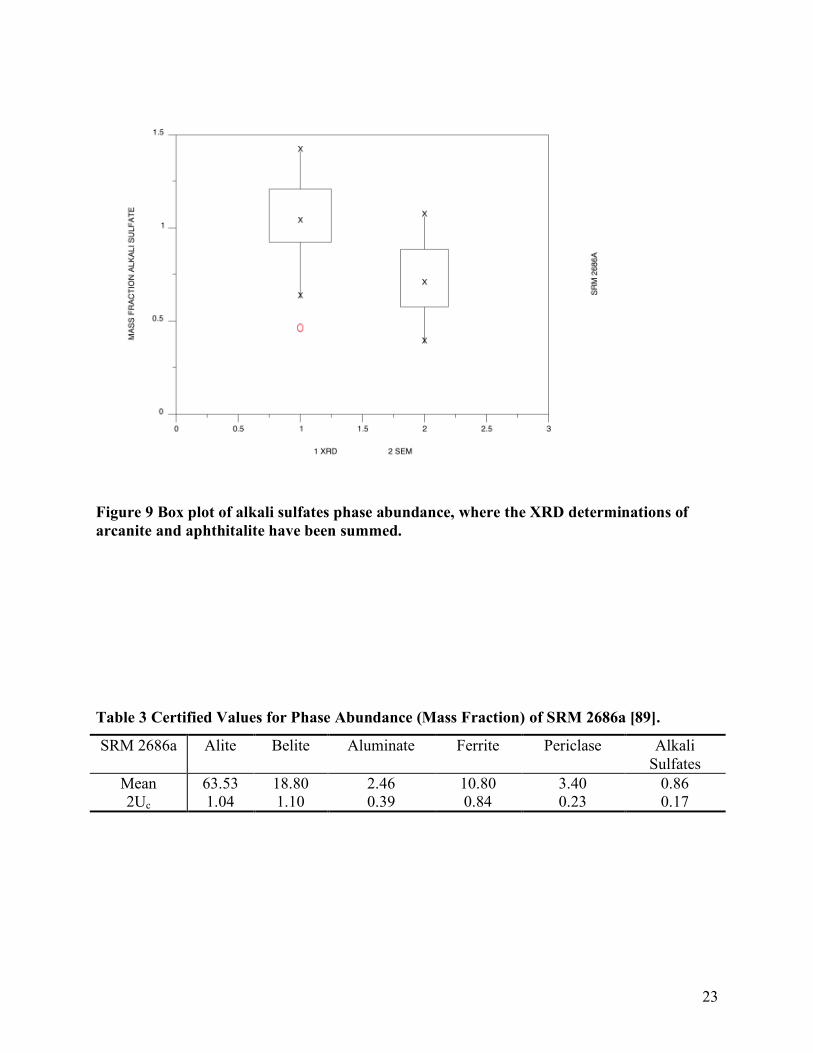
concentrations were both 2.1 %, as indicated by a shared solid line [43]............................ 18 Figure 4 Box plot representation of QXRD and microscopy data on alite phase abundance....... 20 Figure 5 Box plot of belite phase abundance. ............................................................................ 21 Figure 6 Box plots of aluminate phase abundance. .................................................................... 21 Figure 7 Box plot of ferrite phase abundance. ........................................................................... 22 Figure 8 Box plot of periclase phase abundance. ....................................................................... 22 Figure 9 Box plot of alkali sulfates phase abundance, where the XRD determinations of arcanite

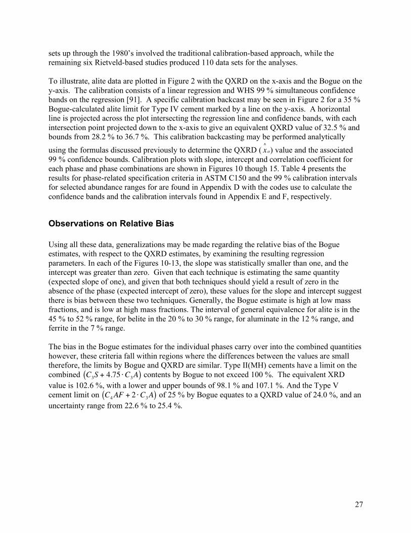
and aphthitalite have been summed. .................................................................................. 23 Figure 10 Alite calibration showing the Bogue (y) and QXRD (x) data pairs, regression and 99 %

confidence bands on the regression. Back casting the Type V 35 % Bogue alite value through the regression line and confidence bands and projecting it down to the x-axis provides the equivalent QXRD value of 32.5 % with a low and high bounds of 28.2 % and 36.7 % .............................................................................................................................. 28

Figure 11 Belite calibration showing the Bogue (y) and QXRD (x) data pairs, regression and 99 % confidence bands on the regression. .............................................................................. 29

Figure 12 Aluminate calibration showing the Bogue (y) and QXRD (x) data pairs, regression and 99 % confidence bands on the regression. ......................................................................... 30

Figure 13 Ferrite calibration showing the Bogue (y) and QXRD (x) data pairs, regression and 99 % confidence bands on the regression. .............................................................................. 31

Figure 14 Calibration for the heat of hydration limit for Type II(MH) cements (C3S + 4.75·C3A 100) showing the Bogue (y) and QXRD (x) data pairs, regression and 99 % confidence bands on the regression. .................................................................................................... 32

Figure 15 Calibration the sum of aluminate and ferrite for Type V, sulfate resistant cements, showing the Bogue (y) and QXRD (x) data pairs, regression and 99 % confidence bands on the regression. ................................................................................................................... 33

8

Introduction R.H. Bogue established the basis for calculating cement phase composition from a bulk chemical analysis in 1929 during a Portland Cement Association Fellowship at the National Bureau of Standards [1]. This study established the relationship between the principal oxides in a cement clinker, CaO, SiO2, Al2O3, Fe2O3, MgO, SO3, and the primary (pure) phases Ca3SiO5 (alite), Ca2SiO4 (belite), Ca3Al2O6 (aluminate), Ca4Al2Fe2O10 (ferrite), and MgO (periclase), using a chemical mass balance. Although it was recognized that portland cements also contained additional minor components like alkalis, titanium, manganese, and phosphates in relatively low concentration (typically less than 2 %), the phases that incorporated them were not known at that time, so these minor phases were not included the calculations. The need to correct for the content of free lime, insoluble residue, and loss on ignition were recognized as significant, but are not typically applied. Regarding the accuracy of the method, Bogue observed the following:

“The accuracy of the computations depends on the correctness of both the postulations and the analytical values. The postulations as given represent the best available information, but are subject to revision and extension as has been pointed out. The general correctness of the analytical values will vary with the conditions of the test and the personal factor.”

The Bogue equations, as they eventually became known, were incorporated in the ASTM specification for portland cements in 1940, and have been used for the subsequent 70 years for process control, cement classification, and specification compliance. The accuracy of the Bogue calculations has been evaluated by comparison to direct determination methods. The Long-Time Study (LTS) in 1948 [2] compared Bogue calculation estimates to composition estimates based on light microscopy. This study found that bias in phase estimation emanated from a number of sources: a) need for corrections for free lime, insoluble residue, and loss on ignition, b) mineral phases and oxides other than the principal ones listed previously, c) the assumption that the phases are pure, and d) the lack of equilibrium during cooling, resulting in other phases being formed, as had already been pointed out by Bogue [3]. Hofmänner [4] demonstrated not only a difference between the methods, but also a difference in phase composition of clinkers having the same elemental content, but different maximum burning temperatures (Table 1). Taylor [5] asserts that the greatest source of bias is the incorporation of minor elements into the major phases, and he developed corrections to the Bogue calculations accounting for the effect. Although the need to account for this by incorporating new information from clinker phase chemistry has been recognized, the Bogue calculations in ASTM C150 remain essentially the same as in 1929.

9

Alite Belite Aluminate Ferrite

1400 °C 1470 °C Bogue Potential

1400 °C

1470 °C

Bogue Potential

1400 °C

1470 °C

Bogue Potential

1400 °C

1470 °C

Bogue Potential

37.8 50.8 31.7 43.4 31.3 40.6 11 11.2 14 6.5 6.3 10

40.7 43.8 38.8 39.5 40.6 35.8 1.3 1 4.1 17.5 14.6 17.6

44 54.6 39.7 44.7 37.2 40.9 6.6 5.1 8.8 3.8 2.3 7.6

48.4 58.9 48.6 39.3 31.7 33.1 0.5 0.5 2.3 11.4 8.7 13.4

67.2 82.6 55.3 9.5 2 19.2 16.3 12.3 12.9 6.3 2.6 8.9

70.2 77.8 64.7 8.1 4.5 12.1 0.5 2.6 3 20.5 14.4 16.8

60.1 73.1 67.3 27 14.6 15.4 0.5 0.5 1.9 11.8 10.1 12.4

71.6 76 67.3 16.3 14 13.9 8 7.5 9.3 2.1 0.5 6.1

Table 1: The dependence of phase concentration on temperature is seen in a comparison of phase estimates from light microscopy and Bogue calculations, from data published by Hofmänner [4].

Direct Methods for Phase Analysis Direct methods, such as microscopy and X-ray powder diffraction are alternatives to the indirect approach of estimating phase composition using chemical analyses. The light microscope, adopted from the geological and metallurgical sciences by LeChatelier in 1887 for the examination of portland cement clinkers, provided the first direct examination and descriptions of clinker composition and texture [6]. The microscope has been used extensively for research and clinker evaluation in the plant, and quantitative analysis [7,8]. By 1960, the microscopy technique had matured and no major advances were noted by Nurse [9] aside from the development of the point-counting method, which facilitated direct quantitative estimates. Campbell [10] provides a recent overview of the application of microscopy to clinker characterization and analysis, while ASTM C1356 details a method for estimating phase fractions by a point-count analysis [11,12]. Point-counting is practical only for clinker analysis as cements are generally too fine-grained for light microscopy and that point-counting can be very time consuming.

Early Applications in Powder Diffraction X-ray powder diffraction was initially used in 1927 by E.A. Harrington to index pure phases related to their studies of cements [13]. A subsequent paper by L.T. Brownmiller and R.H. Bogue used X-ray powder diffraction to examine portland cements to assess the forms and types of phases [14]. At that time multiple theories existed on the true forms of the clinker phases. X-ray powder diffraction provided a means to directly determine the phase composition, particularly for clinkers with textures too fine to be easily resolved by light microscopy. Patterns

10

of synthesized pure phases were compared to the patterns of 28 commercial clinkers. Matches were made for patterns of tricalcium silicate, the beta form of dicalcium silicate, tricalcium aluminate, ferrite, and magnesia (periclase, most likely), with free lime to the industrial clinkers. No evidence of calcium silicate-lime solid solutions with excess free lime was found, which was the prevailing thought in some circles at the time [14]. The potential for quantitative analysis was mentioned but not explored in that study. These studies employed Debye-Scherrer cameras, which used strips of film exposed with the intersection of the diffracted beam. Data analysis involved measuring line position and intensity either through visual estimation, or an optical device. The improved instrumentation through development of the electronic detector and improved X-ray optics by William Parrish in 1947 resulted in an instrument suitable for industrial use [15]. Since its development, the commercial X-ray powder diffractometer has become increasingly common for characterization of clinker, cements, and for hydration products, as well as in the geological sciences for qualitative and quantitative analysis of rocks. The development of powder diffraction as a quantitative method traces its origins to mine dust analysis in the later 1930’s, with the basis of the process relating intensities to mass concentrations described in Klug and Alexander [16]. Copeland and Bragg applied powder diffraction in the analysis of calcium hydroxide in hydration products, where they devised a scheme to decompose overlapping diffraction peaks to address the peak intensity measurement difficulties [17]. They later combined the internal standard method for powder diffraction analysis with a chemical analysis to quantitatively measure the four principal phases in portland cements [18]. They found little systematic difference between Bogue potential phase compositions for alite and ferrite, but that the Bogue method underestimated belite and over estimated the aluminate phase [18]. They also determined that cements contained essentially no glass, as had been thought from microscopy studies up to that time [19]. The International Symposium on the Chemistry of Cement in 1960 contained numerous examples on X-ray powder diffraction for the examination of clinker and cements. High-temperature XRD was used to characterize phase equilibria in systems relevant to cements [9]. Two quantitative methods for phase analysis were described by Midgley, et al. [20], the first being a modification of the Bogue calculations based upon estimates of the ferrite phase composition from XRD data. The second method describes a calibration-based XRD analysis where mixtures of clinker phases and an internal standard (potassium bromide) are prepared, diffraction peak intensities are measured on replicate specimens, and a calibration is established through plotting the ratio of peak intensities of each phase to internal standard against the mass fraction of each phase. Peak intensity measurement posed some difficulty, especially in regions where there was substantial peak overlap, and where a phase was present in low concentration. They did report coefficients of variation of 5 % for alite, 11 % for belite, 3 % for aluminate, and 6 % for ferrite. Subsequent discussion by Kantro et al. [21] further described the analysis problems and their methodologies for calibrations, including resolving diffraction peaks, measurement of the ferrite peak positions, selection of suitable silicate peaks, and selection of an appropriate internal standard. They also illustrated their XRD method and combined XRD/chemical analysis described in [18].

11

A.E. Moore reported on one of the first inter-laboratory tests on X-Ray powder diffraction, microscopy, and classical chemical analysis of portland cements in 1964 [22]. While they did not use a standardized method, allowing individual lab protocols, they made the following observations: 1) the ferrite phase is measured reasonably accurately followed by the aluminates and 2) the silicates pose additional difficulty due to polymorphism and the potential need for references and calibrations for each polymorph. The problems posed in peak intensity measurement were mentioned, establishing a background, decomposing overlapping peaks, and peak area measurement. Whole-pattern methods and the application of a computer were in development and were considered to provide a means to address these difficulties. An early application of computers for automation and data analysis [23,24] where a standard powder diffractometer was automated, including a sample changer. The output was digitized, rutile was used as an internal standard, and a pattern-fitting seheme was used to extract pattern intensities using standard patterns calculated from a set of 26 cements. This approach was unique in three areas: 1) the automation, 2) the pattern-fitting scheme, and 3) the estimation of the standard reference patterns for each phase from a set of cements. This approach was used successfully for the next 20 years by a number of institutions by comparing the unknown to diffraction patterns of individual phases or set of cements of known compositions [25,26,27]. Yamaguchi and Takagi [28] summarized the development of methods for analysis of clinker, noting that key difficulties lie in the measurement of pattern intensities and the inherent variability of the individual phase diffraction patterns. Aldridge published a series of papers on chemical, microscopy, and X-ray methods of analysis of clinker and cement and in the first report [29], he applied the pattern-fitting procedure of Berger et al. [24] to a set of 37 cements and found that while the precision of the analyses were similar to that of the Bogue method, the accuracy was poorer than Bogue calculated values and that analyses of cements from another country were poor. However, this conclusion was based upon a regression analysis of alite, aluminate and fineness against strength. The accuracy may have also been limited by the XRD calibrations and calculation of standard patterns using Bogue-calculated values for their standard cements. Aldridge coordinated an interlaboratory study involving nine laboratories with six cements [30] finding between lab standard deviations (1s) of 7 %, 5 %, 2 %, and 2 %, respectively for alite, belite, aluminate and ferrite, showing little change from the Moore study ten years previous [22]. From this study and a summary of the microscopy, Bogue and XRD analysis program [31], Aldridge considered that no suitable method was available for determination of the phase composition of cement. The major source of error was considered to be the difficulties involved in calibration due to the variability of phase chemistry. A recommendation was made for evaluating the source of calibration errors. These conclusions are similar to that made in subsequent papers on XRD, microscopy and Bogue estimates [32,33].

Developing a Standardized Test Method for Powder Diffraction Analysis Clinker and cement diffraction analyses involve a large number of phases, resulting in a complicated diffraction pattern that can be difficult to decompose into the constituent phases successfully. The first step is a complete qualitative analysis. The traditional means of phase identification is to generate a table of peak positions and relative intensities and search the ICDD

12

database [34] manually using the Hanawalt index or through an interactive search-match routine typically provided with the instrument. The number of phases and peak overlaps typically makes this approach difficult, so an alternative approach is necessary. The concept of key, or diagnostic, diffraction peaks for identification was incorporated into ASTM C 1365 [45] to aid in phase identification. A list of key resolvable diffraction peaks for most common phases in a clinker or cement may be used for initial identifications; confirmation then is accomplished using the ICDD database. There will be some differences in peak positions relative to those in the ICDD database, reflecting chemical and structural variability. A more comprehensive listing of commonly-occurring phases in cements is provided in Appendix A. Selective extractions are a useful tool to produce concentrated mixtures of specific phase groups and for developing optimized control files. Diffraction analysis on these extraction residues serves multiple purposes: 1) improved qualitative analysis as a result of concentration and elimination of interfering phase patterns, 2) the ability to refine the diffraction refined values using patterns with fewer interferences, 3) an additional quantitative estimate of the phases, if a quantitative extraction was performed, and 4) establishing an improved model for each phase that can serve as a starting point for subsequent refinements of more complex mixtures. Details on selective extractions may be found in [35,36] and in Appendix B. X-ray powder diffraction became more widely applied to clinker and cements and a number of novel analytical methods for quantitative analysis evolved [37]. In 1980 ASTM subcommittee C1.23 on compositional analysis established a task group on X-ray diffraction analysis to develop a standard test method for powder diffraction analysis of clinker and cements. The efforts of this task group have produced a number of publications on the performance of QXRD on cement clinker and cements [38,39,40,41,42]. XRD measurements are subject random error and a lab-specific systematic error (bias) [43]. Four factors contribute to test variability: 1) the operator, 2) the equipment, 3) equipment calibration, and 4) the testing environment [44]. The ASTM definition of precision is “the closeness of agreement among test results obtained under prescribed conditions” [44]. This is expressed as repeatability (within-laboratory, sr), which excludes the four factors and reproducibility (between-laboratory, sR), which includes the four factors. Both measures represent standard deviations of replicate analyses. From the sr and sR, limits on the difference between two test results may be calculated, designated as the 95 % repeatability (r) and reproducibility (R) by multiplying the appropriate standard deviation by the factor 2*96.1 [44]. A summary of the initial ASTM work on the interstitial phases (aluminates, ferrite, and periclase) was provided in [40] where known, compounded test mixtures were used to assess precision and bias. Within-lab precision of 1.1% and between-lab precision of 1.7%, on a whole clinker basis was calculated. The mean values from the participants closely mirrored the known values, leading to a conclusion of no apparent bias. An important test was the suitability of using a laboratory-synthesized phase for developing a calibration for an industrial clinker phase. It is much easier to compound mixtures of known phase composition from pure, laboratory-synthesized phases but differences in diffraction peak positions and breadth, reflecting compositional and structural differences may result in them poorly-representing like phases in an industrial product. One set of data on the three NIST SRM

13

clinkers agreed reasonably well with the existing clinker reference values, leading to an observation that while chemical substitution affected peak positions and relative intensities, synthetic standards were suitable for calibrations for a range of clinkers. The efforts of the ASTM QXRD task group culminated in the first standard test method for X-ray powder diffraction analysis of cements, ASTM C 1365, Standard Test Method for Determination of the Proportion of Phases in Portland Cement and Portland-Cement Clinker Using X-ray Powder Diffraction Analysis [45,46]. The principles of X-ray powder diffraction and quantitative analysis is described with an emphasis on clinker and cements by Struble and Graf [47] and by Roode-Gutzmer and Ballim [48]. The results of the inter-laboratory studies mentioned demonstrated utility of applying X-ray powder diffraction for qualitative and quantitative analysis of cements. The primary difficulty for most laboratories was measurement of the individual intensities of key diffraction peaks for quantitative analysis. Early application of peak profile fitting to clinker and cement was difficult due to the substantial peak overlap, the limited refinement range and subsequent uncertainty in estimating a true background. The measurement error was dampened through replicate analyses and measurement, and an unrealistic constraint of equal peak shape characteristics for most of the phases. The application of pattern-fitting [49], similar to that initially described by Frohnsdorff and coworkers [23,24,25] demonstrated a significant improvement in measurement precision over peak profile fitting using the same raw data sets. A problem with this approach when using a single reference pattern is in accommodating for slight differences between reference and unknown pattern phase lattice parameters and peak shapes, which affect the calculated pattern intensity values. Specimen displacement error results from the powder not being co-planer with the specimen holder surface and is the most significant error in diffraction analysis [50]. While a displacement error appears to have little effect, if any, on relative peak intensity, the peak shift accompanying a specimen displacement error will complicate qualitative analysis for reasons mentioned earlier. Gutteridge [27] used a set of reference patterns for each phase, selecting those that provide the lowest residual error in the fit for each phase.

Application of the Rietveld Method to Clinker and Cements The application of the Rietveld method [51,52] provided a means to accommodate the difficulties facing quantitative XRD analysis of clinker and cement. This approach employs a least-squares refinement to minimize the difference between a measured X-ray powder diffraction pattern and a calculated pattern based upon crystal structure, instrument and specimen effects. The addition of the refinement of structural effects now allows accommodation for the influences of chemical and structural variability on the diffraction pattern including peak shape, peak positions, and relative intensities, and the data collection error of specimen displacement, reflected as pattern shift. An excellent introduction to the Rietveld method of powder diffraction analysis is provided by Young [53], where the process is described as “whole-pattern-fitting structure refinement”. A particularly useful section is provided in [53] on refinement strategy that users will find useful in improving their analyses. A description of the method more specifically directed toward cements may be found in references 47 and 48.

14

The number of phases and significant overlapping of their patterns may result in strong correlations between variables, which may confound the refinement process. Keeping the refinement to variables for background, scale, lattice parameters, peak shape, and selectively for preferential orientation helps keep the correlation problems to a minimum. Refinement for site occupancy (aluminum – iron ratios) in the ferrite phase can improve the fit, with only a minor variation in the calculated mass fraction. Selective extraction analyses are considered to provide improved results over those based upon a whole clinker or cement. Examples of selective extractions using the NIST SRM clinkers may be found in Pritula et. al and Lundgaard and Jons [54,55]. Taylor and Aldridge [56] published one of the first papers on clinker analysis by the Rietveld method. They showed that the alite pattern dominates that of the mixture and that the remaining phases have their major diffraction peaks within a region between 35º and 40º 2-Θ, also overlapped by strong alite peaks. They considered the selection of a good alite profile important for a successful refinement and utilized a peak (hkl) file they felt both provided a good fit to alite and reduced computing time. Motzet et al. [57] utilized XRD Rietveld analysis along with light microscopy to examine clinkers with lime saturation factors around 100, finding that factors in excess of 100 do not always contain free lime, but do contain higher alite and lower belite mass fractions. Möller [58] emphasized the need to develop optimized control files to facilitate the analysis. This stems from the complexity of the diffraction patterns from both the number of phases and the complicated patterns produced by many of the phases. The importance of the selection of the alite structure was noted, with the monoclinic models producing the best fits. Taylor [5] notes that the monoclinic form is the most prevalent alite form in industrial clinkers. A comparison of the quantitative results on a set of NIST SRM clinkers demonstrated high precision and low bias and the possibilities for automation for the cement plant were discussed. The NIST SRM clinkers have been invaluable for the development of the XRD method. Their phase abundance values were certified based upon the combined results of light microscopy and XRD, and more recently the addition of scanning electron microscopy with image analysis. Comparisons between the certified values and XRD measurements have demonstrated good agreement in numerous studies [59,60,61,62]. The application of high-resolution synchrotron powder diffraction by [63] suggests that multiple types of alite may exist in clinkers. This may stem from zoning in crystals that is inferred from microscopy studies of etched surfaces, but the lower-resolution laboratory XRD instruments may not resolve these features. De Noirfontaine et al. [64] developed an averaged model to accommodate the presence of M1 and M3 alite in clinker that was considered to be suitable for laboratory powder diffractometers and industrial clinkers. Developing improved structural models by Rietveld analyses are demonstrated in [65,66,67] for alite, and for tricalcium aluminate polymorphs in [68], and [69]. In the latter study, the key conclusion was that the structural models of the cement phases were adequate for accurate quantitative analysis. This is consistent with the conclusions of Struble [39] on the suitability of synthetic phases in earlier studies and suggests that refinement of parameters other than those mentioned previously (atom positions and vibrational parameters) is not necessary for a

15

successful quantitative analysis. In a study on gypsum [70], they found that the structure models refined from the disordered powdered gypsum were better for quantitative XRD those that derived from single crystal studies, reflecting the inherent disorder in gypsum found in the industrial cements. The closer the initial models are to the refined values, the faster, and more likely the refinement will settle on the appropriate values. The application of XRD for industrial process control and the prospects of automation resulted in papers ranging from use of XRD for clinker analysis and plant control as well as XRD application in the characterization of supplementary cementitious materials like slag and fly ash [71,72,73,74]. Plant installations and analysis automation provided a rapid, independent method for quantitative analysis for plotting trends in mineral fractions, including the calcium sulfates, monitoring free lime content, and for predicting properties such as strength development and sulfate durability [75,76,77,78]. Two issues that are receiving more attention are particle statistics for representative sampling and the potential for an amorphous component in clinker and cement. Cements are considered too coarse for proper sampling for diffraction analyses, and the X-ray interaction volume for clinker phases being approximately less than 20 µm. Mitchell et al. [79] examined the effects of particle size and instrument optics that affect the sampling area on precision and while the coarser powders exhibited poorer precision, the quantitative results were significant only for the aluminate phase. Consideration of only particle size does not consider that most particles are poly-phase, and that the interstitial phase crystal sizes are typically smaller than the larger grains. These findings are similar to data in our lab, where the coarse-ground SRM data exhibit a greater propensity for preferred orientation or heterogeneity, but the quantitative results on replicated samples average to be similar to those of more finely-ground powders of the same SRM. The presence of an amorphous component in clinker and cements has been considered in XRD studies that utilize an internal standard [80,81,82,83,84]. This revives the thought from earlier microscopical studies that glass may be present in clinkers, especially those that were quickly cooled. The microscopical analyses in these studies may have been a mis-identification of the isotropic cubic aluminate [5]. Taylor notes that SEM and XRD studies do not support the presence of significant amounts of glass and that studies of clinkers quenched in water resulted in glass formation, but the same clinkers did not form glass when quenched in air. A second potential source is thought to be amorphization of crystalline phases in the grinding process. Intense grinding to achieve particle sizes below 10 µm, considered ideal for XRD analyses, can result in a broadening of the diffraction peaks of the phases. If a significant amount of amorphous material is present in a cement, a broad amorphous diffraction hump is present in the pattern. Absent this indication, the addition of an internal standard is necessary to identify the presence and quantify the concentration of an amorphous fraction. Rietveld results are normalized to 100 % for the phases included in the refinement. Given that amorphous phases do not produce a diffraction pattern, they are not included in the quantitative estimate with a subsequent bias. While the mass fraction estimates are not correct in this case, the mass fraction ratios are correct. The internal standard is a phase not normally present in the cement that is added in a known proportion, homogenized, and included in the refinement. If amorphous material is present, the content of the internal standard will be over-

16

estimated in the refinement. Using the mass fraction ratios and the known mass of internal standard the correct mass estimates of each phase (and internal standard) may be calculated. The difference from 100 being the amorphous content. The selection of internal standard and mass addition is important as the corundum used in a number of these studies may potentially be overestimated due to microabsorption. Better absorption matches for cements and fly ash are zincite and corundum, respectively. This area needs more systematic work to develop a standardized procedure, especially with the prospect of more additions to cements. The NIST SRM clinkers were used to develop a precision statement for ASTM C 1365 in a subsequent inter-laboratory study with five participants and additional data taken from published papers that analyzed the SRM clinkers. A provisional statement was developed based upon the analysis of these data where the within-laboratory standard deviation for all phases averaged 0.84 %. Subsequently, results of two properly conducted tests by the same operator should not vary more than 2.4%. The multi-laboratory standard deviation was found to be 1.54 %, and results of two properly conducted tests on the same clinker by two different laboratories should not differ from each other by more than 4.3 % [85]. While XRD results appear to have lower precision than X-ray fluorescence bulk oxide data, the ultimate uncertainty upon transformation of the bulk oxide values into phase estimates is roughly similar to that of diffraction measurements [86]. Bias is the difference between the test result and the true value. Bias is difficult to discern from inter-laboratory studies, even with certified reference materials or known mixtures. The dominance of the four variability factors, as seen in the larger reproducibility values and suggests improvements in the test method are possible with more control on the process. Given the ASTM test method also covers portland cements, an inter-laboratory study involving eleven laboratories using cements compounded using the SRM clinkers was initiated. Plots of the triplicate replicate data eleven laboratories are shown for cement mixture #1 in line charts, providing a visual assessment of the within-laboratory repeatability and between-laboratory reproducibility. The plots of Figures 1 - 3 show the eleven laboratories’ results with three replicate measurements per lab, connected by a line segment for cement mixture 1. The color-coded solid line indicates the known value and the dashed line a consensus mean value for that constituent. The consistency of results within each lab (repeatability) and the wider variation between labs (reproducibility) is apparent from these plots. The anti-correlation between alite and belite is seen for most participants and a similar effect may be occurring between ferrite and aluminate. Aluminate is consistently over estimated and the ferrite phase is underestimated relative to the known values, possibly reflecting either a method bias, or a bias in the SRM values. The light microscopy values for aluminate for this fine-grained clinker were low relative to the XRD values in certification, possibly reflecting the difficulty in discerning this fine-grained constituent [87]. Laboratories 6 and 11 were excluded as outliers in the calculations for the silicate phases. These data allowed calculations of repeatability and reproducibility, as shown in Table 2, where the within-laboratory (s-within) and between-laboratory (s-between) standard deviations expressed as mass percents. The 95 % difference between duplicate values (d2s), are also shown. Following ASTM convention, results of two properly conducted tests by the same operator should not vary more than ‘r’ while results of two tests on the same clinker or cement by two different laboratories should not differ from each other by more than ‘R’ [46]. The precision

17

measures and an additional bias measure were incorporated into qualification criteria when using the NIST SRM clinkers. The bias criterion is based upon prediction intervals (95 %), designed to bracket values of a mean of k (= 2, 3, 4) future measurements of each phase. The mean result of a phase for a qualification data set should differ from the known value of a certified reference material by no more than the value shown for the number of replicates used. This ensures that the lab’s performance is similar to that of the collective performance of the interlaboratory participants (minus outliers), and is a unique approach in setting limits to laboratory bias. A more recent inter-laboratory study that utilized a pair of known, compounded mixtures and portland cements was conducted by León-Reina et. al [88]. They found estimates for alite to be low and belite to be high. The aluminate and ferrite values were slightly lower, while the calcite and gypsum values were slightly higher. They concluded that the individual results were within one or two standard deviations of the known values, regardless of the structure models and refinement strategies used, indicating that the structure models are adequate for quantitative analysis for the compounded known mixtures. Repeatability values were not calculated but reproducibility values, recalculated as d2s, were slightly greater than in the ASTM interlaboratory study described earlier. This may stem from a number of sources, the lack of a prescribed data collection and analysis procedure, and differences in identification criteria and exclusion of outliers.

Figure 1 Silicate estimates of cement mix 1 with three replicates for each of 11 labs [46].

18

Figure 2 Interstitial phase replicate data for cement mix 1[43]

Figure 3 Calcium sulfate phase replicate data for cement mix 1. Bassanite and anhydrite concentrations were both 2.1 %, as indicated by a shared solid line [43].

19

Table 2 Within-laboratory (s-within) and between-laboratory (s-between) standard deviations expressed as mass percents and maximum difference between duplicates for within- and between-laboratories, r and R. [43].

Repeatability Within-Laboratory

Reproducibility Between-Laboratory

Phase s-within r (d2s) s-between R (d2s) alite 0.74 2.04 2.23 6.18 belite 0.64 1.77 1.41 3.91 aluminate 0.47 1.31 0.74 2.05 ferrite 0.49 1.36 0.95 2.63 periclase 0.23 0.63 0.32 0.89 arcanite 0.22 0.60 0.41 1.13 gypsum 0.21 0.59 0.58 1.62 bassanite 0.39 1.08 0.81 2.24 anhydrite 0.27 0.74 0.63 1.75 calcite 0.99 2.73 0.50 1.50

Microscopy and XRD: Certification of SRM 2686a The certification of SRM 2686a clinker for phase abundance provides an opportunity to examine two unique direct methods with two independent operators making determinations on clinker phase abundance. XRD with Rietveld analysis (n=16) and scanning electron microscopy with image analysis (n=10) were used to establish phase abundance values on a crushed, blended clinker sample. Errors in the microscopy-derived values may stem from incorrect classifications upon segmentation and inability to distinguish between very finely divided interstitial phases while the uncertainty in the XRD measurements will stem from any incomplete identification of minor and trace phases, difficulties in the refinement process, microabsorption, and the inability to identify and control correlations between refined variables. These data were used to establish consensus means and uncertainties for this SRM (Table 3) and provide some insight into relative bias between these two direct methods. Box plots illustrate the comparison between the XRD and SEM data, through graphical comparison of the alignment or mis-alignment of median values and differences in interquartile ranges. Important features of the box plot are:

1. the width of each box is proportional to sample size, 2. the median value is used for its resistance to outliers, and is identified by the X, 3. the interquartile range ("middle half") of the data are represented by the body of the box, 4. the extremes (minimum and maximum) are represented by the ends of the straight lines

projecting out of the box, and 5. circles outside the extremes of each box represent outliers.

20

Overall, a comparison between these two methods shows quite a close agreement in phase abundance estimates. The XRD data for alite (Figure 4) and belite (Figure 5) exhibit greater precision than the microscopy data and, while the boxes overlap, both phase median estimates by XRD are lower than those by microscopy. The heterogeneity of the phase distribution and the small per-field sampling area is responsible for the greater variability in the microscopy. The XRD values for aluminate values (Figure 6) and ferrite (Figure 7) are slightly higher than the microscopy. Particularly for the ferrite phase, this is opposite what would be anticipated if microabsorption was a source of bias. Mitigating factors may be the fine grinding or perhaps the fine crystal size also reduces the propensity for microabsorption-induced bias. Ferrite and periclase estimates (Figure 8) exhibit reasonably close agreement between XRD and microscopy. The alkali sulfate (Figure 9) represent a sum of arcanite and aphthitolite as these phases were not distinguished in the SEM imaging.

Figure 4 Box plot representation of QXRD and microscopy data on alite phase abundance.

21

Figure 5 Box plot of belite phase abundance.

Figure 6 Box plots of aluminate phase abundance.

22

Figure 7 Box plot of ferrite phase abundance.

Figure 8 Box plot of periclase phase abundance.

23

Figure 9 Box plot of alkali sulfates phase abundance, where the XRD determinations of arcanite and aphthitalite have been summed. Table 3 Certified Values for Phase Abundance (Mass Fraction) of SRM 2686a [89].

SRM 2686a Alite Belite Aluminate Ferrite Periclase Alkali Sulfates

Mean 2Uc

63.53 1.04

18.80 1.10

2.46 0.39

10.80 0.84

3.40 0.23

0.86 0.17

24

Relating Bogue-based Specification Criteria to XRD Measurements With an established ASTM standard for direct phase determination by QXRD, knowledge of comparability, or relative bias, to the Bogue-calculated values is important for acceptance of QXRD values in the ASTM C 150 standard cement specification. Mixed results have often been obtained in different studies comparing direct methods to Bogue-calculated values. One broad generality is that alite is estimated low while aluminate is estimated high by Bogue relative to direct measures [5]. A distinct advantage of QXRD analysis is the more complete mineralogical description of the cement, important because the calcium sulfates and alkali sulfates, not accounted for by the Bogue calculations, can influence the hydration and rheological characteristics. To incorporate this measurement technique into ASTM C150 [90] for classifying cements, there must be a means of estimating equivalent QXRD values for each Bogue-related limit for cement classification in ASTM C150. Toward this end, statistical analyses of published and internal data consisting of companion Bogue and QXRD estimates of cement phase are used to establish the most likely linear relationship between these two measurement techniques for alite, belite, aluminate, ferrite, and for the combinations (C3S+4.75·C3A) and (C4AF+2·C3A) used to characterize heat of hydration and sulfate resistance, respectively. The resulting calibration is presented in this report, establishing bounds for the QXRD values corresponding to the Bogue limits given in ASTM C150 Table 1. The goal of the following section is to establish the link between Bogue-calculated phases and direct-determined phase composition through calibration.

Calibration Calculation Method Table 1 of ASTM C150 contains ten specification criteria based upon single phases, or combinations of phases. These limits have a long-standing historical performance basis using the Bogue-calculated values, yet any relative bias with respect to QXRD would preclude the same specification criteria being used for QXRD-based measurements. One approach to rectifying this problem is to re-evaluate the performance criteria related to each specification limit in light of QXRD data. This has the potential advantage of offering a more complete and accurate accounting of the cement phase constituents. A database on performance using the CCRL cements is in development at this time at NIST, but more work is needed to complete these new phase criteria. Another means of establishing a relationship between two distinct measurement techniques is calibration [91]. Inverse regression, or calibration, estimators and associated uncertainties have wide applicability in scientific and engineering applications [92]. In this case we wish to quantitatively relate measurements made using different measurement systems: the indirect Bogue calculations and the direct X-Ray powder diffraction analyses. The calibration of XRD phase compositions against traditional Bogue values provides equivalent XRD values for cement for the ASTM C150 Table 1 criteria based upon existing specification limits.

25

To perform the calibration for each cement phase considered, paired data (x, y) are plotted with the x-value being the direct measurement (QXRD) and the y-value being the indirect measurement (Bogue). An ordinary least squares regression line (

!

b

"

+ mx"

) is fit to the paired data, resulting in a calibration line between Bogue and QXRD. From this calibration line, each Bogue-based phase limit in ASTM C150 (y0) can be converted to an equivalent QXRD estimated value (

!

x

"

o) by applying a simple inversion estimator:

!

!! "=

m

byx oo

The uncertainty in the calibration is characterized by the Working-Hotelling-Scheffé (WHS) [93,94] simultaneous confidence bands on the regression. In this study, 99 % WHS bands are used, meaning that the likelihood that the true calibration line lies in the region defined by the hyperbolic WHS bands is 99 %. The resulting expression for the uncertainty of

!

x

"

o (ux) obtained on backcasting through the bands is [95,96]:

!

ux =

2 " F2,n#2$( )%

& 1

n1#'( ) +

y0# y ( )

2

m& 2

Sxx

(

)

* *

+

,

- -

m&

1#'( )

1 2

The quantity

!

" is a correction due to uncertainty in the estimated slope:

!

" =F2,n#2

$ %& 2

m

& 2

SXX

The quantity

!

F2,n"2

#( ) is the appropriate F distribution percent point, SXX is notation for

!

xi" x ( )

i=1

n

#2

(sum of the squared deviations of the X values from the mean), and

!

"^

is the

residual standard deviation from the linear least squares fit. Because coefficient of variation

!

CV

^

((standard error)/(expected value)) of the estimated slope

!

m

^

!

CV (m) ="#

m

#

Sxx

is small ( < 0.10) for all the calibrations in this study, indicating that the regression line slopes are sufficiently accurate, the quantity ε can be safely set equal to zero in the above equation [91].

Assumptions and Limitations on the Calibration Calculation Method The assumptions in the calibration are that 1) the straight-line model, with non-predetermined slope and intercept, is appropriate for Bogue phase estimates as a function of corresponding QXRD measurements and 2) that it is not inappropriate to model linearly data that aggregates

26

multiple cement types. Given that both Y and X measurements are attempting to assess the same underlying physical quantities (phase mass fractions), a straight line was considered reasonable. The intercept is not automatically set to zero because while at true phase concentration zero, both Bogue and QXRD estimates should be zero, there is no guarantee that they will be. Further, empirical fitting to data at hand gives intercept estimates that are statistically distinguishable from zero (95 % confidence). The appropriateness, or utility, of trying to equivalence C150 to QXRD employing data that aggregates over cement Type is somewhat more questionable. It is done here for purposes of numerical/statistical methodology exposition, and to enable quick evaluation of potential equivalence over a wide range of cement characteristics. In practice, it is more likely to be useful to repeat these sorts of analyses on specific cement types one at a time, or specific categories within type one at a time. An issue in the use of Ordinary Least Squares (OLS) technology in fitting and exercising linear models is the error structure in X and Y [97]. Theoretical OLS requires no error in X, all existing error in Y, which, in practice, is rarely achieved. If the magnitude of (relative) error in X approximates magnitude of (relative) error in Y alternative, Errors in Variables (EIV), fitting technology should be employed. A rule of thumb says that if rel-err(Y) > rel-err(X) by approximately an order of magnitude or better, it is still appropriate to employ OLS, rather than EIV, methodology. As yet unpublished work on actual uncertainties in Bogue phase estimates indicates that they can fluctuate around 10 % for the silicates and 6 % for the interstitial phases, whereas for QXRD the corresponding figure is on the order of about 2.5 % and 1 %, respectively so the use of OLS here is justified. The simultaneous WHS confidence bounds for the lines considered, through which C150 uncertainties are backcast to obtain the "calibration" uncertainties on the corresponding QXRD measurements, are bounds on a "true" entity, in this case on the "true" straight line which the least squares-fitted line estimates. Because the WH hyperbolic bands, which take into account uncertainty both in slope and intercept determination, bound the "true" line, they are not designed to, nor do they, bracket 99 % of the observed data. Bands designed to accomplish that would be 99 % - 99 % tolerance bands (e.g., Lieberman-Miller tolerance bands), which if computed and plotted would be observed to bracket 99 % of the observed data, at every X point along the curve, with 99 % "probability" [98]. For calibration purposes, however, backcasting through the best estimate of "truth" available would appear to be the appropriate way to proceed.

Calibration of Relevant Phases and Quantities Ten data sets, dating from 1960 to the present, containing both QXRD and Bogue values for portland cements and clinkers were selected for this study [Error! Bookmark not defined., 99, 100, 29, 28, 30, 31, 101, 102, 103, 104]. These studies were supplemented by unpublished QXRD data on the Cement and Concrete Reference Laboratory (CCRL) proficiency cements and other cements analyzed at NIST, providing 194 data pairs for the four principal phases and internal data from the CCRL proficiency test cements at NIST. Eight studies comprising 84 data

27

sets up through the 1980’s involved the traditional calibration-based approach, while the remaining six Rietveld-based studies produced 110 data sets for the analyses. To illustrate, alite data are plotted in Figure 2 with the QXRD on the x-axis and the Bogue on the y-axis. The calibration consists of a linear regression and WHS 99 % simultaneous confidence bands on the regression [91]. A specific calibration backcast may be seen in Figure 2 for a 35 % Bogue-calculated alite limit for Type IV cement marked by a line on the y-axis. A horizontal line is projected across the plot intersecting the regression line and confidence bands, with each intersection point projected down to the x-axis to give an equivalent QXRD value of 32.5 % and bounds from 28.2 % to 36.7 %. This calibration backcasting may be performed analytically using the formulas discussed previously to determine the QXRD (

!

x

"

o) value and the associated 99 % confidence bounds. Calibration plots with slope, intercept and correlation coefficient for each phase and phase combinations are shown in Figures 10 though 15. Table 4 presents the results for phase-related specification criteria in ASTM C150 and the 99 % calibration intervals for selected abundance ranges for are found in Appendix D with the codes use to calculate the confidence bands and the calibration intervals found in Appendix E and F, respectively.

Observations on Relative Bias Using all these data, generalizations may be made regarding the relative bias of the Bogue estimates, with respect to the QXRD estimates, by examining the resulting regression parameters. In each of the Figures 10-13, the slope was statistically smaller than one, and the intercept was greater than zero. Given that each technique is estimating the same quantity (expected slope of one), and given that both techniques should yield a result of zero in the absence of the phase (expected intercept of zero), these values for the slope and intercept suggest there is bias between these two techniques. Generally, the Bogue estimate is high at low mass fractions, and is low at high mass fractions. The interval of general equivalence for alite is in the 45 % to 52 % range, for belite in the 20 % to 30 % range, for aluminate in the 12 % range, and ferrite in the 7 % range. The bias in the Bogue estimates for the individual phases carry over into the combined quantities however, these criteria fall within regions where the differences between the values are small therefore, the limits by Bogue and QXRD are similar. Type II(MH) cements have a limit on the combined

!

C3S + 4.75 "C

3A( ) contents by Bogue to not exceed 100 %. The equivalent XRD

value is 102.6 %, with a lower and upper bounds of 98.1 % and 107.1 %. And the Type V cement limit on

!

C4AF + 2 "C

3A( ) of 25 % by Bogue equates to a QXRD value of 24.0 %, and an

uncertainty range from 22.6 % to 25.4 %.

28

Figure 10 Alite calibration showing the Bogue (y) and QXRD (x) data pairs, regression and 99 % confidence bands on the regression. Back casting the Type V 35 % Bogue alite value through the regression line and confidence bands and projecting it down to the x-axis provides the equivalent QXRD value of 32.5 % with a low and high bounds of 28.2 % and 36.7 %

29

Figure 11 Belite calibration showing the Bogue (y) and QXRD (x) data pairs, regression and 99 % confidence bands on the regression.

30

Figure 12 Aluminate calibration showing the Bogue (y) and QXRD (x) data pairs, regression and 99 % confidence bands on the regression.

31

Figure 13 Ferrite calibration showing the Bogue (y) and QXRD (x) data pairs, regression and 99 % confidence bands on the regression.

32

Figure 14 Calibration for the heat of hydration limit for Type II(MH) cements (C3S + 4.75·C3A 100) showing the Bogue (y) and QXRD (x) data pairs, regression and 99 % confidence bands on the regression.

33

Figure 15 Calibration the sum of aluminate and ferrite for Type V, sulfate resistant cements, showing the Bogue (y) and QXRD (x) data pairs, regression and 99 % confidence bands on the regression.

34

Table 4 Equivalent X-ray Powder Diffraction Values for C 150 Bogue specifications, with 99 % Confidence Interval about the QXRD.

Phase

Cement Type

ASTM C150 Limits (Bogue)

Low

QXRD Xo

High

Alite Type IV maximum 35 28.2 32.5 36.7

Belite Type IV minimum 40 39.8 43.0 46.2

Aluminate Type II,

Type II(MH)

maximum 8 6.5 7.3 8.0

Aluminate Type III maximum 15 16.2 18.8 21.5

Aluminate Type IV maximum 7 4.9 5.6 6.4

Aluminate Type V maximum 5 1.2 2.3 3.5

C3S+4.75·C3A Type II(MH)

!

"100 98.1 102.6 107.1

C4AF+2·C3A Type IV

!

" 25 22.6 24.0 25.4

Aluminate Type III optional maximum 8 6.5 7.3 8.0

Aluminate Type III optional maximum 5 1.2 2.3 3.5

Summary X-ray powder diffraction analysis has been used in the cement industry since the mid-1920’s. The application of the Rietveld analysis procedure to clinker and cements addresses two primary problems in powder diffraction analysis, pattern decomposition, intensity measurement, and tailoring standards to the material. Results of this approach produce significantly improved precision compared to the more traditional peak intensity measurements and calibration curves. Precision for within- and between-laboratory have been calculated in three inter-laboratory studies on clinker and cements, and have been used to establish precision and qualification criteria for ASTM C 1365. The measurement of amorphous components, such as fly ash and slag, present the need for additional work in development of a test protocol. The cement industry has successfully performed phase content estimates via the Bogue calculations for the past 70 years. However, errors long acknowledged to be inherent to the calculations have limited their use in accurately and completely characterizing the actual mineralogical compositions. Directly determined phase analysis of cements has been sought because of its potential for greater accuracy and more complete accounting of the actual phase compositions, which should provide a better basis for relating mineralogical composition to performance characteristics and improving predictive capability for cements. A new knowledge

35

base of performance characteristics relative to phase composition should be developed using these data, but the initial step is to relate X-Ray powder diffraction and Bogue-derived phase estimates through statistical calibration of current ASTM C150 limits. Scatter plots provide a visual representation of the relationship between the two different methods of phase estimation. Calibration is accomplished through linear regression and Working-Hotelling 99 % confidence limits of the regression line. Calibrations have been established for the four principal phases used in the Bogue calculation, alite, belite, aluminate, and ferrite, and additionally for combinations of phases that reflect limits for sulfate resistance for Type II and II(MH) cements, heat of hydration for Type II(MH) cements, and for Type V sulfate resisting cements. These data are used to establish equivalent QXRD values for ASTM C150 Table 1 phase composition-related limits, allowing both techniques for phase estimation to be used in assessing the compliance of a portland cement.

Acknowledgements Stefan Leigh and Andrew Rukhin provided assistance with the calibrations while division reviewers Ken Snyder and Chiara Ferraris provided review comments. Robin Haupt of the Cement and Concrete Reference Laboratory (CCRL) provided the CCRL cements and proficiency test reports with the bulk chemical data. The research reported in this paper (PCA R&D Serial No. 3084a) was conducted by the National Institute of Standards and Technology, with the sponsorship of the Portland Cement Association (PCA Project Index No. 07-08). The contents of this paper reflect the views of the authors, who are responsible for the facts and accuracy of the data presented. The contents do not necessarily reflect the views of the Portland Cement Association.

36

Appendix A: Selective Extractions for Clinker and Cement

Potassium Hydroxide/Sugar Extraction (KOH/sugar) The KOH/sugar extraction dissolves the interstitial phases of aluminate and ferrite leaving a residue of silicates and minor phases such as periclase. First, prepare an extraction solution of 7.5 g of KOH and 7.5 g of sucrose in 75 ml of water. Then stir about 2 g of powdered cement in a 95 °C KOH/sugar solution for one minute (no longer). Filter the solution using a 0.45 µm filter and Buchner funnel, wash residue with 50 ml of water followed by 100 ml of methanol, dry the residue at 100 °C, and store in a vacuum desiccator. Vacuum filtering fine clinker or cement powder extraction suspensions can often be difficult. To minimize problems, do not exceed the recommended extraction times. Alternatively, extract and filter a coarser particle size sample. Because of the much larger particle size, care must be taken to ensure that the extraction has removed all the intended phases and that preferred orientation in the resulting diffraction pattern is recognized.

Salicylic Acid/Methanol Extraction (SAM) The SAM extraction is used to dissolve alite, belite, and free lime leaving a residue of interstitial phases, aluminate and ferrite, as well as minor phases, periclase and alkali sulfates. For cements, the calcium sulfate phases are also found in the residue. The SAM solution is prepared by dissolving 20 g salicylic acid in 300 ml of methanol. Stir about 5 g of powdered cement in a stoppered flask containing 300 ml of SAM solution for two hours. Allow the suspension to settle for about 15 minutes then vacuum filter using a 0.45 µm filter and Buchner funnel. Wash the residue with methanol, dry at 60 °C, and store in a vacuum desiccator. Preservation of the calcium sulfate hydrate form is important for cements so drying should be done at no more than 60 °C to allow for evaporation of the methanol. Gutteridge [36] used a modified SAM method combined with the KOH/sugar extraction to obtain residues enriched in belite. In this procedure, the mass of salicylic acid was adjusted to five times the mass of alite as estimated by the Bogue calculation.

Nitric Acid/Methanol Extraction This extraction dissolves the silicates and aluminates leaving a residue of ferrite and periclase (if present). Ten grams of ground clinker stirred in 500 ml of 7 % nitric acid in methanol for 30 minutes dissolves the silicates and aluminates.

37

Appendix B: Diffraction Peak positions and relative intensities for phases commonly found in Portland Cements (Cu Kα) from the ICDD Database [34]. Bold-face indicates a key (diagnostic) peak, with little overlap with strong peaks of other phases.

d-Spacing Two-Theta Phase 7.627 11.593 gypsum (100) 7.249 12.200 C4AF (45) 5.997 14.759 bassanite (80) 5.970 14.827 triclinic C3S (12) 5.953 14.869 triclinic C3S (12) 5.927 14.935 triclinic C3S (12) 5.927 14.935 mono. C3S (12) 5.610 15.784 γC2S (19) 5.107 17.350 C3Ao (10) 4.917 18.026 aphthitalite (10) 4.659 19.033 thenardite (71) 4.640 19.112 α´C2S (30) 4.316 20.561 γC2S (45) 4.284 20.717 gypsum (100) 4.253 20.869 langbeinite (30) 4.235 20.959 C3Ac (6) 4.222 21.024 langbeinite (25) 4.188 21.197 langbeinite (16) 4.175 21.264 arcanite (28) 4.158 21.352 arcanite (23) 4.091 21.706 aphthitalite (30) 4.079 21.770 C3Ac (12) 4.059 21.879 γ C2S (20) 3.900 22.783 αC2S (20) 3.886 22.866 triclinic C3S (10) 3.838 23.156 thenardite (17) 3.817 23.285 γC2S (509) 3.810 23.328 α´C2S (30) 3.799 23.397 gypsum (17) 3.764 23.617 γC2S (119) 3.744 23.745 arcanite (18) 3.670 24.231 aphthitalite (20) 3.653 24.346 C4AF (16) 3.497 25.450 anhydrite (100) 3.468 25.666 bassanite (40) 3.462 25.711 langbeinite (12) 3.424 26.002 C3Ao (11) 3.385 26.307 arcanite (13) 3.379 26.354 γC2S (25) 3.370 26.426 α´C2S (30) 3.313 26.889 langbeinite (95) 3.271 27.241 langbeinite (80) 3.263 27.309 langbeinite (80) 3.225 27.637 langbeinite (100)

3.180 28.036 thenardite (52) 3.153 28.281 langbeinite (18) 3.114 28.643 langbeinite (18) 3.077 28.995 thenardite (55) 3.065 29.111 gypsum (75) 3.056 29.198 triclinic C3S (60) 3.045 29.306 bassanite (10) 3.040 29.355 triclinic C3S (55) 3.038 29.375 M1 C3S (50) 3.036 29.395 mono C3S (40) 3.034 29.415 m1 C3S (50) 3.025 29.504 triclinic C3S (65) 3.025 29.504 mono C3S (75) 3.011 29.645 γC2S (80) 3.002 29.736 bassanite (80) 3.000 29.756 arcanite (77) 2.985 29.909 triclinic C3S (25) 2.974 30.022 triclinic C3S (18) 2.972 30.043 M1 C3S (20) 2.968 30.084 mono C3S (12) 2.968 30.084 M1 C3S (20) 2.965 30.115 triclinic C3S (20) 2.961 30.157 mono C3S (25) 2.940 30.378 aphthitalite (75) 2.902 30.785 arcanite (100) 2.894 30.872 γC2S (25) 2.886 30.960 arcanite (53) 2.880 31.026 langbeinite (18) 2.876 31.070 βC2S (21) 2.872 31.115 gypsum (45) 2.870 31.137 α´C2S (30) 2.850 31.361 anhydrite (29) 2.838 31.497 aphthitalite (100) 2.813 31.784 βC2S (22) 2.813 31.784 bassanite (100) 2.810 31.819 αC2S (80) 2.790 32.053 βC2S (97) 2.788 32.077 triclinic C3S (100) 2.788 32.077 gypsum (10) 2.786 32.101 langbeinite (45) 2.784 32.124 C4AF (25) 2.784 32.124 thenardite (100) 2.782 32.148 βC2S (100) 2.776 32.220 free lime (36) 2.775 32.231 M1 C3S (100)

38

2.775 32.231 langbeinite (50) 2.773 32.255 mono C3S (85) 2.767 32.327 triclinic C3S (70) 2.754 32.484 triclinic C3S (65) 2.750 32.533 γC2S (70) 2.750 32.533 langbeinite (45) 2.747 32.569 mono C3S (45) 2.747 32.569 M1 C3S (40) 2.745 32.593 βC2S (83) 2.743 32.618 M1 C3S (60) 2.743 32.618 langbeinite (45) 2.740 32.655 α´C2S (100) 2.737 32.691 mono C3S (75) 2.736 32.704 triclinic C3S (60) 2.728 32.802 γC2S (100) 2.717 32.939 βC2S (30) 2.714 32.976 C3Ao (65) 2.714 32.976 bassanite (10) 2.710 33.026 αC2S (100) 2.698 33.178 C3Ac (100) 2.692 33.254 C3Ao (100) 2.684 33.356 gypsum (35) 2.680 33.407 α´C2S (75) 2.673 33.497 C4AF (35) 2.647 33.836 thenardite (52) 2.644 33.875 C4AF (100) 2.618 34.222 triclinic C3S (60) 2.612 34.303 triclinic C3S (90) 2.610 34.330 βC2S (42) 2.607 34.371 M1 C3S (70) 2.605 34.398 M1 C3S (80) 2.603 34.425 mono C3S (100) 2.590 34.604 γC2S (14) 2.576 34.798 C4AF(17) 2.517 35.640 arcanite (13) 2.514 35.684 γC2S (25) 2.499 35.906 arcanite (15) 2.494 35.980 gypsum (11) 2.458 36.526 triclinic C3S (12) 2.458 36.526 aphthitalite (10) 2.455 36.572 γC2S (17) 2.448 36.680 βC2S (12) 2.442 36.774 aphthitalite (16) 2.430 36.962 periclase (10) 2.422 37.088 arcanite (25) 2.409 37.296 βC2S (13) 2.405 37.360 free lime (100) 2.402 37.408 βC2S (18) 2.385 37.685 arcanite (13) 2.374 37.866 arcanite (17)

2.360 38.100 α´C2S (30) 2.339 38.455 triclinic C3S (15) 2.329 38.627 triclinic C3S (20) 2.329 38.627 thenardite (25) 2.329 38.627 aphthitalite (14) 2.328 38.644 anhydrite (20 2.325 38.696 γC2S (10) 2.323 38.725 M1 C3S (10) 2.319 38.800 M1 C3S (20) 2.315 38.870 triclinic C3S (25) 2.315 38.870 mono C3S (20) 2.280 39.491 βC2S (22) 2.280 39.491 triclinic C3S (11) 2.270 39.672 α´C2S (10) 2.268 39.709 bassanite (10) 2.230 40.415 α´C2S (30) 2.229 40.433 arcanite (19) 2.220 40.605 αC2S (40) 2.218 40.643 gypsum (15) 2.209 40.816 anhydrite (20) 2.205 40.893 C3Ao (20) 2.205 40.893 arcanite (14) 2.203 40.932 C3Ac (10) 2.196 41.068 langbeinite (12) 2.195 41.088 triclinic C3S (75) 2.189 41.206 βC2S (51) 2.184 41.304 M1 C3S (40) 2.181 41.364 mono C3S (60) 2.180 41.383 α´C2S (30) 2.179 41.403 triclinic C3S (17) 2.179 41.403 M1 C3S (40) 2.171 41.563 triclinic C3S (11) 2.169 41.603 M1 C3S (10) 2.166 41.663 M1 C3S (10) 2.164 41.704 βC2S (13) 2.164 41.704 mono C3S (15) 2.163 41.724 triclinic C3S (11) 2.162 41.744 M1 C3S (10) 2.136 42.276 bassanite (20) 2.109 42.844 langbeinite (18) 2.105 42.930 periclase (100) 2.093 43.188 langbeinite (20) 2.088 43.297 arcanite (25) 2.085 43.362 gypsum (25) 2.082 43.428 arcanite (25) 2.073 43.626 gypsum (15) 2.051 44.118 C4AF(35) 2.050 44.141 βC2S (14) 2.041 44.346 aphthitalite (45) 2.036 44.461 langbeinite (14)

39

2.026 44.692 βC2S (15) 2.024 44.738 γC2S (13) 2.020 44.832 α´C2S (30) 2.019 44.855 βC2S (15) 2.017 44.902 langbeinite (20) 2.009 45.091 langbeinite (14) 1.994 45.449 triclinic C3S (10) 1.982 45.740 M1 C3S (10) 1.981 45.764 βC2S (20) 1.973 45.960 mono C3S (10) 1.940 46.788 αC2S (60) 1.937 46.865 M1 C3S (10) 1.933 46.968 M1 C3S (10) 1.930 47.045 α´C2S (30) 1.930 47.045 mono C3S (13) 1.928 47.097 C4AF(35) 1.919 47.331 C3Ao (35) 1.908 47.621 γC2S (60) 1.908 47.621 bassanite (10) 1.908 47.629 C3Ac (30) 1.900 47.834 α´C2S (30) 1.899 47.860 gypsum (16) 1.893 48.022 βC2S (24) 1.891 48.076 C3Ao (19) 1.889 48.130 arcanite (12) 1.882 48.320 γC2S (15) 1.879 48.402 gypsum (12) 1.869 48.678 anhydrite (16) 1.865 48.789 thenardite (36) 1.847 49.296 bassanite (30) 1.814 50.255 C4AF(45) 1.813 50.284 γC2S (11) 1.811 50.344 gypsum (13) 1.802 50.613 γC2S (12) 1.778 51.345 gypsum (12) 1.764 51.783 mono C3S (55) 1.757 52.004 mono C3S (30) 1.756 52.036 γC2S (12) 1.754 52.100 γC2S (14) 1.749 52.260 anhydrite (11)

1.748 52.292 anhydrite (10) 1.732 52.813 bassanite (10) 1.701 53.852 free lime (54) 1.693 54.127 bassanite (20) 1.689 54.266 γC2S (35) 1.680 54.581 thenardite (13) 1.665 55.114 bassanite (10) 1.656 55.439 aphthitalite (12) 1.648 55.732 anhydrite (15) 1.637 56.139 aphthitalite (10) 1.635 56.214 γC2S (20) 1.580 58.355 α´C2S (30) 1.580 58.355 αC2S (40) 1.578 58.436 C4AF (14) 1.563 59.052 C3Ao (35) 1.560 59.177 αc2s (20) 1.558 59.261 C3Ac (24) 1.552 59.513 thenardite (10) 1.551 59.555 C3Ao (20) 1.538 60.110 C4AF (14) 1.527 60.588 γC2S (12) 1.488 62.351 MgO (52) 1.472 63.106 γC2S (16) 1.450 64.177 free lime (16) 1.421 65.649 arcanite (10) 1.418 65.806 aphthitalite (10) 1.412 66.121 arcanite (12) 1.388 67.415 free lime (16) 1.346 69.818 C3Ao (12) 1.321 71.338 C4AF (12) 1.216 78.611 periclase (12) 1.155 83.658 bassanite (10) 1.078 91.212 bassanite (10) 1.075 91.539 free lime (16) 0.982 103.330 free lime (12) 0.941 109.885 periclase (17) 0.859 127.460 periclase (15) 0.813 142.687 free lime (10) 0.801 148.161 free lime (16)

40

Appendix C. XRD and Bogue data pairs. Alite Belite Aluminate Ferrite XRD Bogue XRD Bogue XRD Bogue XRD Bogue CCRL 62.2 69.5 14.7 3.9 2.8 5.9 12.9 9.9 Stutzman 57.1 62.9 16.5 10.5 6.8 7.3 13.9 9.6 56.3 52.2 19.9 18.5 6.2 8.1 9.8 9.2 58.4 60.4 19.2 13.8 4.9 7.0 11.6 9.7 63.7 64.5 12.2 8.8 5.4 7.2 11.6 10.5 64.1 61.5 11.3 10.8 8.9 11.0 8.1 7.3 59.3 54.2 20.2 18.9 2.9 7.5 11.6 10.5 65.3 55.3 9.9 21.7 3.8 4.3 9.1 8.8 64.2 62.3 17.9 11.6 4.7 7.6 9.8 10.2 51.7 54.7 24.1 16.6 10.3 11.4 6.1 6.7 52.9 52.5 21.1 20.9 3.9 4.2 11.1 10.2 56.9 58.2 17.0 15.8 8.2 5.5 11.1 9.1 49.3 62.2 21.8 10.5 10.3 10.2 6.0 6.1 58.7 51.7 11.1 19.8 5.9 7.4 15.5 11.0 57.7 57.5 18.4 15.0 3.5 7.5 12.8 11.1 55.1 51.9 21.1 19.2 1.8 6.6 14.5 10.7 62.0 58.6 13.5 14.9 12.7 8.4 4.2 8.4 50.4 54.8 23.9 16.6 3.0 6.4 14.8 12.9 54.8 46.0 16.6 28.7 6.4 3.5 12.9 11.2 64.5 51.5 5.9 13.7 9.9 6.6 7.2 9.4 48.6 52.5 18.7 18.6 11.6 7.7 7.4 10.2 54.9 53.8 15.7 18.6 9.9 9.2 6.5 7.7 Crumbie, 79.4 65.2 7.5 16.1 5.1 5.1 7.9 11.0 Walenta, 79.5 68.2 7.1 13.0 5.3 5.4 7.4 10.8 Fullmann 82.9 64.6 4.0 16.6 12.2 13.2 0.1 3.1 85.1 68.1 4.1 13.0 9.5 12.9 0.3 3.0 72.9 65.0 13.2 16.3 6.4 5.0 7.4 11.0 76.3 68.2 10.3 12.6 6.2 5.1 7.0 10.9 77.5 65.6 8.3 15.7 12.7 13.0 1.3 3.1 77.5 69.0 8.1 12.5 12.8 13.1 1.2 3.0 Neubauer 66.9 64.7 18.4 19.0 9.1 8.5 5.6 7.8 ICCC data 60.7 58.8 24.8 24.5 8.1 8.8 6.4 7.9 71.2 68.3 15.3 15.6 7.6 8.5 5.9 7.0 77.1 75.1 9.1 9.0 7.7 8.2 6.1 7.7 71.1 67.9 14.7 16.0 8.8 8.5 5.4 7.6 65.0 61.9 21.6 22.2 7.6 8.0 5.8 7.9 55.9 54.7 30.5 29.3 7.8 8.0 5.8 8.0 61.4 60.3 24.1 23.8 8.7 8.4 5.8 7.5 68.7 68.4 17.2 15.8 8.2 8.2 5.9 7.6 68.8 67.5 17.4 16.7 7.7 8.1 6.1 7.7 68.0 68.1 18.3 16.0 7.4 8.0 6.3 7.9 67.0 65.5 18.1 18.3 9.1 8.4 5.8 7.8

41

Alite Belite Aluminate Ferrite XRD Bogue XRD Bogue XRD Bogue XRD Bogue Stutzman 64.0 60.7 13.3 15.7 1.3 3.8 14.0 12.2 PSU/NIST 56.1 59.5 17.6 13.2 3.7 6.4 12.7 9.7 59.7 62.4 15.4 9.7 11.4 11.7 5.0 4.9 67.8 59.1 7.0 14.4 8.1 10.0 7.0 5.9 53.7 54.5 16.3 17.5 8.6 10.0 10.4 8.8 57.2 57.2 12.9 14.4 5.4 9.6 12.2 8.8 55.8 52.0 18.1 19.5 5.3 9.3 11.5 7.7 60.5 58.3 12.4 16.5 5.9 7.5 8.5 7.5 60.0 53.7 14.3 15.7 3.5 9.5 13.9 7.9 53.7 47.2 20.6 23.3 3.2 6.7 12.5 9.7 61.8 58.9 13.7 16.7 4.6 5.8 11.8 8.8 55.5 56.5 18.3 17.8 5.9 7.2 11.6 9.5 59.5 57.8 17.3 14.3 3.4 7.8 13.5 7.9 63.4 60.1 11.0 14.2 6.6 9.5 6.2 4.6 57.8 55.1 19.2 19.4 4.3 7.2 12.1 7.4 62.3 59.2 14.3 11.9 10.4 10.6 5.6 6.0 60.3 61.1 15.3 12.0 4.9 9.8 10.6 8.8 60.9 60.6 12.6 13.6 1.7 7.4 13.8 9.8 56.2 52.0 13.6 19.2 6.0 7.3 10.3 8.9

Aldridge '82 69.0 66.5 15.0 12.4 6.5 7.0 7.0 7.4

72.0 63.0 12.0 8.7 8.0 6.5 4.4 5.7 62.0 59.3 19.0 17.2 6.8 5.7 10.0 11.0 49.0 43.9 31.0 33.6 5.7 5.9 10.5 10.6 59.0 58.3 21.0 15.2 9.2 6.0 6.4 9.1 61.0 54.3 26.0 27.0 7.1 12.0 1.3 0.7

Aldridge '82 40.3 47.4 6.8 7.0

61.0 70.0 8.2 7.3 49.1 56.1 4.9 5.4 38.4 40.1 5.4 4.0 52.0 61.5 10.1 10.4 60.6 66.5 5.1 8.6 62.2 73.0 51.7 59.3 40.7 43.9 49.2 58.3 55.6 54.3

Aldridge '75 63.6 53.3 15.3 24.0 8.4 7.9 5.7 5.4 51.9 49.1 29.2 31.7 4.7 6.4 7.3 5.7 52.2 53.5 26.9 27.9 7.3 6.6 6.6 5.9

66.1 63.6 13.0 15.5 4.7 6.1 9.3 7.1 60.3 63.0 15.3 12.8 11.8 10.5 5.7 6.7 59.3 56.2 18.4 18.3 9.3 10.3 6.2 5.8 72.1 68.5 4.0 7.0 4.1 5.4 12.9 10.6 68.9 67.4 8.1 9.9 4.7 4.5 11.4 11.0 75.9 73.5 1.2 3.2 3.5 3.7 12.5 11.9 67.6 69.0 8.5 7.8 3.9 4.0 13.1 12.1

42

Alite Belite Aluminate Ferrite XRD Bogue XRD Bogue XRD Bogue XRD Bogue 66.3 72.7 11.0 5.0 6.3 3.5 9.5 11.8 63.2 62.3 14.4 16.5 7.4 6.9 8.1 7.8 57.0 51.6 24.2 24.1 2.3 3.2 9.4 11.9 48.7 51.0 31.2 28.2 2.1 0.3 11.2 11.9 49.1 43.0 31.6 36.0 2.6 2.7 9.8 10.9 47.8 49.8 32.5 28.7 2.2 2.6 10.6 10.6 50.3 45.2 25.7 29.8 4.5 6.0 12.6 11.7 47.0 40.7 30.5 34.5 2.7 1.0 12.9 15.4 47.4 39.1 30.0 36.9 4.1 4.0 11.6 10.6 52.6 46.8 24.7 30.4 4.3 5.1 11.5 9.4 49.8 65.6 28.8 10.4 3.4 4.8 11.1 10.3 45.9 46.4 30.0 26.5 8.6 5.6 8.6 10.0 45.6 42.0 30.5 27.5 7.9 6.3 9.0 9.6 Yamaguchi & 55.0 52.0 26.0 26.0 9.0 9.0 9.0 8.0 Takagi '68 55.0 42.0 26.0 34.0 7.0 10.0 11.0 10.0 58.0 57.0 24.0 24.0 7.0 7.0 11.0 10.0 49.0 48.0 33.0 31.0 3.0 7.0 14.0 11.0 A.E. Moore 48.0 52.5 36.0 30.5 1.3 2.5 9.7 11.5 64 46.0 52.5 38.0 31.5 1.6 2.0 9.8 11.0 38.0 40.5 44.0 40.5 0.0 1.3 13.9 13.0 OPC 56.2 54.7 23.9 23.0 6.4 10.4 7.2 7.6 SRPC 56.0 59.6 24.7 19.7 0.5 0.1 13.7 17.6 Midgley '60 65.0 70.0 13.0 7.0 11.5 9.5 8.5 9.2 58.0 66.0 16.0 8.0 3.7 2.5 17.5 18.0 59.0 61.0 11.0 9.1 13.5 15.4 10.5 10.2 56.0 56.0 17.0 17.0 4.8 0.7 17.5 19.0 39.0 34.5 32.0 38.3 4.5 0.9 16.5 19.3 59.0 46.0 16.0 29.0 11.0 9.6 6.4 6.2 53.0 53.0 21.0 22.0 12.1 10.7 8.8 6.3 50.0 36.0 30.0 37.0 14.0 15.0 9.0 10.0 Midgley '60 53.0 47.0 24.0 28.0 9.3 8.4 9.5 9.2 54.0 42.0 24.0 26.0 12.8 12.9 11.0 9.2 49.0 44.0 27.0 32.0 8.3 8.8 6.2 6.6 53.0 48.0 23.0 23.0 14.5 13.1 9.0 7.3 43.0 42.0 30.0 30.0 9.8 10.9 12.5 9.0 60.0 48.0 27.0 29.0 9.7 9.5 7.6 6.3 35.0 26.0 45.0 49.0 8.8 9.2 6.9 6.6 53.0 55.0 23.0 22.0 9.7 9.7 7.5 5.6 55.0 53.0 17.0 18.0 3.6 0.9 17.5 19.6 Kantro '60 60.0 50.0 19.9 22.0 7.6 12.1 9.2 7.2 48.3 45.0 26.0 28.0 7.9 12.6 7.3 7.3 53.8 50.0 29.7 26.0 6.8 10.1 8.3 6.5

43

XRD Bogue XRD Bogue XRD Bogue XRD Bogue Alite Belite Aluminate Ferrite LTS 1960 55.2 42.5 25.1 32.0 3.2 8.2 11.1 9.2 63.5 64.5 13.0 10.0 10.4 12.1 6.0 7.5 58.7 53.5 24.5 21.0 3.9 7.5 11.4 10.7 53.4 52.0 18.5 23.0 7.3 10.4 9.6 9.3 53.2 44.5 26.9 28.0 7.6 13.2 7.6 6.8 49.6 40.0 38.6 41.0 3.6 6.4 10.0 9.7 50.2 41.5 30.4 33.5 2.3 6.6 13.4 11.7 55.5 51.0 23.2 24.0 2.6 3.7 13.3 16.6 50.3 41.0 27.2 29.0 2.2 5.4 14.4 14.8 37.6 34.0 41.8 39.0 0.3 4.7 13.2 14.9 56.7 56.0 16.8 17.0 7.7 10.8 6.3 6.4 58.7 60.0 18.5 13.0 7.0 10.4 8.7 7.7 62.8 64.0 13.9 10.5 3.0 5.7 11.4 10.1 25.6 20.0 52.8 51.0 0.0 4.5 15.0 15.2 33.2 27.0 55.0 55.0 1.3 3.5 10.0 8.2 33.9 25.0 53.7 48.0 2.5 6.2 14.1 13.8 48.2 41.0 35.2 39.0 0.2 3.7 10.1 10.0 WES 29.8 33.0 32.5 37.0 5.1 8.0 19.3 14.0 Cements 56.5 60.0 12.5 17.0 0.9 1.0 13.5 13.0 39.4 50.0 24.5 23.0 1.1 8.0 14.8 9.0 26.6 42.0 46.1 33.0 6.1 3.0 11.7 10.0 Costa 52.5 54.2 27.4 21.7 11.9 11.2 6.4 7.3

51.3 56.0 30.8 19.7 10.3 11.5 6.1 8.0 65.1 58.9 11.2 18.0 14.9 10.0 7.7 9.4 58.6 52.1 19.5 24.5 13.1 9.4 8.1 9.7 65.8 58.8 14.5 17.7 9.9 9.0 9.0 9.5 69.6 67.2 7.8 6.5 7.6 11.2 11.7 8.9 70.4 66.6 11.4 11.4 3.1 6.6 12.3 9.7 71.0 68.7 9.2 11.3 10.5 7.9 9.0 7.8 70.6 63.0 13.3 15.7 2.6 9.0 10.6 7.3 59.7 55.4 16.7 19.7 15.7 11.8 4.2 6.7 64.5 59.7 18.1 18.9 8.5 8.9 6.3 6.0 69.1 67.0 12.3 11.9 2.0 7.0 13.0 8.5 65.1 61.9 21.3 19.4 1.9 3.6 10.3 10.5 65.7 60.6 18.4 16.8 3.7 6.5 11.6 10.1 49.6 45.6 31.6 31.9 6.0 6.4 11.6 10.9 69.3 63.1 7.5 14.3 16.0 11.3 5.8 7.3 47.1 45.4 32.8 27.5 9.0 10.9 8.3 8.1 71.8 72.0 6.0 5.3 6.2 7.1 16.0 12.5 72.5 70.5 4.2 6.9 9.2 7.1 14.1 12.3 66.7 63.1 16.8 18.3 4.7 4.2 6.9 7.4 69.0 60.8 9.3 15.1 11.7 10.5 8.0 7.9

44

XRD Bogue XRD Bogue XRD Bogue XRD Bogue Alite Belite Aluminate Ferrite

58.0 54.0 18.4 22.1 7.7 5.4 13.7 12.9 62.1 61.6 16.9 13.0 10.6 9.4 6.2 7.1 67.9 70.2 14.5 7.6 2.1 5.0 13.2 11.1 62.6 58.0 12.5 16.9 14.5 10.1 9.9 9.6 67.5 63.9 14.0 12.1 2.6 8.1 13.8 10.4 66.0 61.0 15.3 14.9 2.8 8.5 14.1 9.4 52.0 60.5 29.3 18.1 5.8 6.4 12.9 12.7 69.7 65.9 10.3 10.2 6.4 8.3 10.5 8.9 70.5 62.4 8.9 15.1 13.4 10.2 6.5 7.9 73.4 68.3 10.2 11.9 1.6 2.2 13.2 12.2 69.5 69.7 6.9 7.4 5.3 5.9 17.1 13.4 61.1 61.9 20.3 15.5 3.7 6.7 12.7 10.4 62.8 63.2 16.7 11.9 6.7 9.3 11.5 9.1 77.8 69.8 8.6 8.7 3.4 7.6 8.8 7.5 60.8 50.0 19.4 21.5 6.1 8.4 10.1 9.8 62.1 59.0 17.7 16.1 8.1 8.6 9.5 9.9 72.7 63.3 5.9 9.8 4.7 8.0 14.2 10.8 66.3 60.2 12.3 12.8 9.8 9.8 11.2 9.8 71.0 59.1 11.1 17.0 5.3 7.3 11.6 10.0 66.3 60.0 9.6 16.8 15.5 8.6 5.9 9.2 64.0 60.0 10.8 16.9 12.9 9.8 10.8 9.3 64.4 57.1 11.9 17.7 14.5 8.8 8.4 11.3 63.6 57.1 14.1 17.7 6.9 8.8 14.6 11.3 64.2 66.6 18.3 10.7 2.6 6.4 12.2 10.0 63.4 58.6 15.1 17.3 8.7 9.2 11.6 10.0 59.8 55.9 22.4 21.9 5.7 7.8 11.0 10.8

45

Appendix D: Fieller Confidence Intervals

Alite 99 % Confidence Interval Y0 Low Bound Xo High Bound

30.0 21.2 26.3 31.4

31.0 22.6 27.6 32.5 32.0 24.0 28.8 33.5 33.0 25.4 30.0 34.6 34.0 26.8 31.2 35.6 35.0 28.2 32.5 36.7 36.0 29.6 33.7 37.7 37.0 31.0 34.9 38.8 38.0 32.4 36.1 39.9 39.0 33.8 37.4 40.9 40.0 35.2 38.6 42.0 41.0 36.6 39.8 43.0 42.0 38.0 41.0 44.1 43.0 39.4 42.3 45.2 44.0 40.7 43.5 46.2 45.0 42.1 44.7 47.3 46.0 43.5 45.9 48.4 47.0 44.9 47.2 49.5 48.0 46.2 48.4 50.5 49.0 47.6 49.6 51.6 50.0 48.9 50.8 52.7 51.0 50.2 52.1 53.9 52.0 51.6 53.3 55.0 53.0 52.9 54.5 56.1 54.0 54.1 55.7 57.3 55.0 55.4 56.9 58.5 56.0 56.7 58.2 59.7 57.0 57.9 59.4 60.9 58.0 59.1 60.6 62.2 59.0 60.3 61.8 63.4 60.0 61.4 63.1 64.7 61.0 62.6 64.3 66.0 62.0 63.7 65.5 67.4 63.0 64.8 66.7 68.7 64.0 65.9 68.0 70.0 65.0 67.0 69.2 71.4 66.0 68.1 70.4 72.7 67.0 69.2 71.6 74.1 68.0 70.2 72.9 75.5 69.0 71.3 74.1 76.9 70.0 72.4 75.3 78.2 71.0 73.5 76.5 79.6 72.0 74.5 77.8 81.0 73.0 75.6 79.0 82.4 74.0 76.6 80.2 83.8 75.0 77.7 81.4 85.2

46

Belite 99 % Confidence Interval Y0 Low Bound Xo High Bound

5.0 0.0 2.5 5.0

6.0 1.3 3.7 6.0 7.0 2.6 4.8 7.0 8.0 3.9 6.0 8.1 9.0 5.1 7.1 9.1

10.0 6.4 8.3 10.2 11.0 7.7 9.4 11.2 12.0 8.9 10.6 12.3 13.0 10.2 11.8 13.3 14.0 11.5 12.9 14.4 15.0 12.7 14.1 15.5 16.0 13.9 15.2 16.6 17.0 15.1 16.4 17.7 18.0 16.3 17.6 18.8 19.0 17.5 18.7 19.9 20.0 18.7 19.9 21.1 21.0 19.8 21.0 22.2 22.0 20.9 22.2 23.4 23.0 22.1 23.3 24.6 24.0 23.2 24.5 25.9 25.0 24.2 25.7 27.1 26.0 25.3 26.8 28.3 27.0 26.4 28.0 29.6 28.0 27.4 29.1 30.8 29.0 28.5 30.3 32.1 30.0 29.5 31.5 33.4 31.0 30.6 32.6 34.7 32.0 31.6 33.8 35.9 33.0 32.6 34.9 37.2 34.0 33.7 36.1 38.5 35.0 34.7 37.2 39.8 36.0 35.7 38.4 41.1 37.0 36.8 39.6 42.4 38.0 37.8 40.7 43.7 39.0 38.8 41.9 44.9 40.0 39.8 43.0 46.2

47

Aluminate 99 % Confidence Interval

Y0 Low Bound Xo High Bound

1.0 -6.6 -4.3 -2.0 2.0 -4.7 -2.6 -0.6 3.0 -2.7 -1.0 0.7 4.0 -0.7 0.7 2.1 5.0 1.2 2.3 3.5 6.0 3.1 4.0 4.9 7.0 4.9 5.6 6.4 8.0 6.5 7.3 8.0 9.0 8.0 8.9 9.8

10.0 9.5 10.6 11.7 11.0 10.8 12.2 13.6 12.0 12.2 13.9 15.6 13.0 13.5 15.5 17.5 14.0 14.9 17.2 19.5 15.0 16.2 18.8 21.5 16.0 17.5 20.5 23.4 17.0 18.9 22.1 25.4 18.0 20.2 23.8 27.4 19.0 21.5 25.4 29.4 20.0 22.8 27.1 31.4

Ferrite 99% Confidence Interval Y0 Low Bound Xo High Bound

1.0 -4.9 -2.7 0.5 2.0 -3.1 -1.2 0.8 3.0 -1.4 0.3 2.1 4.0 0.3 1.8 3.3 5.0 2.1 3.3 4.6 6.0 3.8 4.8 5.9 7.0 5.5 6.3 7.2 8.0 7.1 7.8 8.5 9.0 8.7 9.3 9.9

10.0 10.2 10.8 11.4 11.0 11.6 12.3 13.0 12.0 12.9 13.8 14.7 13.0 14.2 15.3 16.4 14.0 15.5 16.8 18.1 15.0 16.7 18.3 19.8 16.0 18.0 19.8 21.6 17.0 19.3 21.3 23.3 18.0 20.5 22.8 25.0 19.0 21.8 24.3 26.8 20.0 23.0 25.8 28.5

48

C4AF + 2C3A 99 % Confidence Interval

Y0 Low Bound Xo High Bound 20.0 12.1 14.5 17.0 21.0 14.3 16.4 18.5 22.0 16.5 18.3 20.1 23.0 18.7 20.2 21.8 24.0 20.7 22.1 23.5 25.0 22.6 24.0 25.4 26.0 24.4 25.9 27.4 27.0 26.1 27.8 29.6 28.0 27.6 29.7 31.8 29.0 29.2 31.6 34.0 30.0 30.7 33.5 36.3

C3S + 4.75 C3A 99 % Confidence Interval Y0 Low Bound Xo High Bound

90.0 83.4 87.2 91.0 95.0 90.9 94.9 98.8 100.0 98.1 102.6 107.1 105.0 104.9 110.3 115.6 110.0 111.6 118.0 124.4

49

Appendix E: Dataplot code for Working-Hotelling Confidence Bounds DIMENSION 20 COLUMNS DEVICE 1 aqua device 2 close DEVICE 2 POSTCRIPT . .. READ lab X Y 1 62.2 69.5 1 57.1 62.9 1 56.3 52.2 . . . 14 56.5 60.0 14 39.4 50.0 END OF DATA . .. LET N = NUMBER X LET N2=N-2 LET FUNCTION F1=M*X+B LET FUNCTION F2=M*X2+B FIT Y=F1 LET FVAL=FPPF(.99,2,N2) LET XMIN = MIN X LET XMAX = MAX X LET XINC=(XMAX-XMIN)/50. LET X2 = XMIN XINC XMAX LET Y2 = F2 LET XBAR = MEAN X LET X3 = (X-XBAR)**2 LET SX3 = SUM X3 LET X4=(X2-XBAR)**2 LET X5 = SQRT((1/N)+(X4/SX3)) LET HTLOW1 = Y2-RESSD*SQRT(2*FVAL)*X5 LET HTHI1 = Y2+RESSD*SQRT(2*FVAL)*X5 Capture alite_99_limits.txt LET CC = Correlation x y COMMENT *** F-BASED HOTELLING 99% CONF BOUNDS *** PRINT X2 Y2 HTLOW1 HTHI1 END OF CAPTURE TITLE Working-Hotelling Simultaneous 99% Confidence Bounds Title Case ASIS Title Displacement 1 Title Size 3.5 Label Size 3 tic mark label size 2

50

Title Thickness .75 Label Thickness .75 Frame Thickness .25 Xlabel Case ASIS Ylabel Case ASIS XLABEL X-Ray Powder Diffraction YLABEL ASTM C-150 Y2LABEL Alite Frame Color Black Title Color Black . CHARACTERS BLANK X BLANK BLANK LINES SOLID BLANK SOLID SOLID Line THICKNESS 0.3 0.3 0.3 0.3 LINE COLOR BLUE RED RED BLUE character size 2 2 2 2 2 2 2 2 2 2 2 2 2 2 2 2 2 2 2 2 3 2 2 3 char color blue . PLOT HTLOW1 VS X2 AND PLOT Y VS X AND PLOT Y2 VS X2 AND PLOT HTHI1 VS X2 . .. Exit

51

Appendix F: Dataplot code for Fieller Calibration Confidence Intervals . .. Alite XRD vs Bogue Data from Fieller Plots.xls 2/18/09 . .. DATAPLOT program implementing . .. calibration confidence interval(s) . .. of Fieller (1954) . .. modified for inversion of W-H bands . .. by using sqrt(2*F(0.99,2,n-2) . .. dimension 40 columns device 1 aqua . .. read lab x y 1 62.2 69.5 1 57.1 62.9 1 56.3 52.2 . . . 14 56.5 60.0 14 39.4 50.0 END OF DATA . .. let n = number x . .. fit y= m*x+b . .. let mx = mean x let my = mean y . .. let dx = x-mx let dx = dx**2 let ssx = sum dx for i = 1 1 n . .. delete x y . .. let nm2 = n-2 let ff = fppf(0.99,2,nm2) let e = (ff*(ressd**2))/((m**2)*ssx) . .. let epsrat = (ressd)/(m*(sqrt(ssx))) . .. read y0 30 31

52

32 . . . 74 75 end of data . .. let den = m*(1-e) let num = (1/n)*(1-e)+((y0-my)**2)/((m**2)*ssx) let num = sqrt(num) let numhi = (y0-my)+(sqrt(2*ff))*ressd*num let numlo = (y0-my)-(sqrt(2*ff))*ressd*num let fielhi = mx+(numhi/den) let fiello = mx+(numlo/den) . .. let x0 = (y0-b)/m let onesig = (fielhi-x0)/(2) let relsig = (onesig/x0)*100 . .. capture Falite_99.txt . .. print " *** Y0 *** LO-BOUND *** X0 *** HI-BOUND *** REL-1-SIGMA" print " " print y0 fiello x0 fielhi relsig . .. end of capture exit

53

References 1 R.H. Bogue, Calculation of the Compounds in Portland Cement”, Industrial and Engineering Chemistry, Vol. 1, No. 4, pp. 192-197 2 W. Lerch and C.L. Ford, “Chemical and Physical Tests of the Cements”, in Long-Time Study of Cement Performance in Concrete, Portland Cement Association Bulletin 26, August 1948 3 R.H. Bogue, Calculation of the Compounds in Portland Cement, Paper No. 21, Portland Cement Association Fellowship at the national Bureau of Standards, October 1929 4 F. Hofmänner, Microstructure of Portland Cement Clinker, Holderbank Management and Consulting, Ltd., 1973 5 H.F.W. Taylor, Cement Chemistry, Thomas Telford, 1997 459 p. 6 D.H. Campbell, Microscopical Examination and Interpretation of Portland Cement and Clinker, SP 030, PCA1999 7 L.S. Brown, “Microscopical Study of Clinkers”, in Long-Time Study of Cement Performance on Concrete, Chapter 4, PCA Bulletin 26, pp. 877-923, 1948 8 H. Insley and Van D. Fréchette, Microscopy of Ceramics and Cements, Academic Press, New York, 1955 9 R.W. Nurse, “Phase Equilibria and Constitution of Portland Cement Clinker,” Paper II-1, pp. 9-37, in Proceedings of the Fourth International Symposium on the Chemistry of Cement, Washington, DC, 1960. 10 D.H. Campbell, Microscopical Examination and Interpretation of Portland Cement and Clinker, 2nd ed., Portland Cement Association, 1999, 224 pp. 11 D.H. Campbell and J.S. Galehouse, Quantitative Clinker Microscopy with the Light Microscope, Cement, Concrete and Aggregates, Vol. 13, No. 2 12 C 1356-07 Test Method for Quantitative Determination of Phases in Portland Cement Clinker by Microscopical Point-Count Procedure, Vol. 4.01, ASTM International, West Conshohocken, PA 13 E.A. Harrington, “X-ray Diffraction Measurements on some of the Pure Compounds Concerned in the Study of Portland Cement”, Paper No. 8, PCA Fellowship, 1927; also Am. Jour. Sci. 5th series, Vol. XIII, No. 78, June 1927, pp. 467-479 14 L.T. Brownmiller and R.H. Bogue “The X-ray Method Applied to a Study of the Constitution of Portland Cement”, PCA Fellowship paper No. 24, 1930; also Am. Jour. Sc., Fifth series, Vol. XX, No. 118, October, 1930 pp. 241-264 15 D.K. Smith, William Parrish, 1915-1991, J. Appl. Cryst. (1991) 24 975-977 16 H.P. Klug and L.E. Alexander, X-Ray Diffraction Procedures for Polycrystalline and Amorphous Materials, Wiley, New York, 1974 17 L.E. Copeland and R.H. Bragg, “Quantitative X-Ray Diffraction Analysis,” Anal. Chem., 30, 196, 1958 18 L.E. Copeland, S. Brunauer, D.L. Kantro, E.G. Schulz, and C.H. Weise, “Quantitative Determination of the Four Major Phases of Portland Cement by Combined X-Ray and Chemical Analysis,” Anal. Chem., Vol. 31, No. 9, 1521, September 1959 19 H. Insley and V.D. Fréchette, Microscopy of Ceramics and Cements, Academic Press, New York, 1955, 267 pp. 20 H.G. Midgley, D. Rosaman, and K.E. Fletcher, “X-Ray Diffraction Examination of Portland Cement Clinker,” Paper II-S2, pp. 69-81, in Proceedings of the Fourth International Symposium on the Chemistry of Cement, Washington, DC, 1960. 21 D.L. Kantro, L.E. Copeland, and S. Brunauer, “Quantitative Analysis of Portland Cements by X-Rays,”, pp. 75-80, pp. 69-81, in Proceedings of the Fourth International Symposium on the Chemistry of Cement, Washington, DC, 1960.

54

22 A.E. Moore, “Comparison of the Results Obtained for the Compound Composition of Portland Cements by X-Ray Diffraction, Microscopy, and Wet Chemical Methods,” Analysis of Calcareous Materials, S.C.I. Monograph No. 18, pp. 372-390, 1964. 23 G.J.C. Frohnsdorff and P.H. Harris, “Use of Digital Techniques in the Phase Analysis of Portland Cement by X-Ray Diffraction, Analysis of Calcareous Materials, S.C.I. Monograph No. 18, pp. 320-336, 1964. 24 R.L. Berger, G.J.C. Frohnsdorff, P.H. Harris, and P.D. Johnson, “Application of X-Ray Diffraction to Routine Mineralogical Analysis of Portland Cement,” in Symposium on Structure of Portland Cement Paste and Concrete, Highway Research Board Special Report 90, Washington, D.C., pp. 234-253, 1966. 25 C.M. Ballantyne, “Quantitative Automatic Determination of Cement Compound Composition Using X-Ray Diffraction Techniques,” Cement and Concrete Association Departmental Note 7001, 1968 26 A.E. Moore, “Mineralogical Analysis of Portland Cement by X-Ray Diffraction,” Proc. Soc. Chem. Ind., 18-20, 1970. 27 W.A. Gutteridge, “Quantitative X-Ray Powder Diffraction in the Study of Some Cementitive Materials,” in F.P. Glasser, ed., The Chemistry and Chemically-Related Properties of Cement, Proceedings No. 35, British Ceramic Society, pp. 11-24, 1984. 28 G. Yamaguchi and S. Takagi, “The Analysis of Portland Cement Clinker”, Principal paper I-3, Fifth International Symposium on the Chemistry of Cement, Tokyo, pp. 181-216. 29 L.P. Aldridge, “International Cement Analysis Study. Part 3. Quantitative X-ray Diffraction Analysis of Cements”, Report No. C.D. 2201, Department of Scientific and Industrial Research, New Zealand, 1975, 20 pp. 30 L.P. Aldridge, “Quantitative X-ray Diffraction Analysis of Cements”, Report No. C.D. 2202, Department of Scientific and Industrial Research, New Zealand, 1975, 14 pp. 31 L.P. Aldridge, “International Cement Analysis Study. Part 4: Comparison of Results,” Report No. C.D. 2267, Department of Scientific and Industrial Research, New Zealand, 1978, 18 pp. 32 L.P. Aldridge, “Accuracy and Precision of Phase Analysis in Portland Cement by Bogue, Microscopic and X-Ray Diffraction Methods,” Cement and Concrete Research, Vol. 12, pp. 381-398, 1982. 33 L.P. Aldridge, “Accuracy and Precision of an X-Ray Diffraction Method for Analyzing Portland Cements,” Cement and Concrete Research, Vol. 12, pp. 437-446, 1982. 34 Powder Diffraction Database, International Centre for Diffraction Data, Newtown Square, PA 19073-3273 U.S.A., http://www.icdd.com/ 35 W.A. Klemm and J. Skalney, "Selective Dissolution of Clinker Minerals and Its Applications," Martin Marietta Technical Report 77-32, 30 pp., 1977 36 W.A. Gutteridge, "On the Dissolution of the Interstitial Phases in Portland Cement," Cement and Concrete Research, Vol. 9, pp. 319-324, 1979. 37 L. Struble, “Quantitative X-Ray Diffraction Analysis of Cement and Clinker: A Bibliography,” Cement, Concrete and Aggregates, Vol. 5, No. 1, 1983, pp. 62-29 38 L. Struble and H. Kanare, “Cooperative Calibration and Analysis of Cement Clinker Phases,” NIST IR 89-4164, 34 pp., 1989 39 L.J. Struble, “Cooperative Calibration and Analysis of Cement Clinker Phases, Report 2,” Civil Engineering Studies, Structural Research Series No. 556, University of Illinois, 21 pp., 1990 40 L.J. Struble, “Quantitative Phase Analysis of Clinker Using X-Ray Diffraction, Cement, Concrete, and Aggregates, Winter, 1991, pp. 97-102. 41 P. Stutzman, Development of an ASTM Standard Test Method on X-Ray Powder Diffraction Analysis of Hydraulic Cements, Advances in A-Ray Analysis, Vol. 47, pp. 205-211, 2003

55

42 P. Stutzman, “Powder Diffraction Analysis of Hydraulic Cements: ASTM Rietveld Round Robin Results on Precision”, Powder Diffraction, Vol. 20, No. 2, June 2005 43 W.J. Youden, ‘Statistical Techniques for Collaborative Tests,’ Association of Official Analytical Chemists, Inc., 1973 64 pp. 44 ASTM E 691, ‘Standard Practice for Conducting an Interlaboratory Study to Determine the Precision of a Test Method,’ in Annual Book of ASTM Standards, Vol. 4.01, 2001. ASTM International, West Conshohocken, PA 45 ASTM C 1365-06, “Standard Test Method for Determination of the Proportion of Phases in Portland Cement and Portland –Cement Clinker Using X-Ray Powder Diffraction Analysis, ASTM Book of Standards, Vol. 4.01, ASTM International, West Conshohocken, PA. 46 P. Stutzman and S. Leigh, “Phase Analysis of Hydraulic Cements by X-Ray Powder Diffraction: Precision, Bias, and Qualification”, Journal of ASTM International, Vol. 4, No. 5, paper ID JAI101085, 11 pp., 2007 47 L.J. Struble, L.A. Graf, J.I. Bhatty, “X-Ray Diffraction Analysis”, in Innovations in Portland Cement Manufacturing, Chapter 8.2, J.I. Bhatty, F. M. Miller, and S.H. Kosmatka, eds, PCA SP 400.01, 2004, 1367 pp. 48 Q.I. Roode-Gutzmer and Y. Ballim, “Phase Composition and Quantitative X-Ray Powder Diffraction Analysis of Portland Cement and Clinker,” in Materials Science of Concrete VI, S. Mindess, ed., pp. 1-42, 2001. 49 P.E. Stutzman, “Pattern-Fitting for Quantitative X-Ray Powder Diffraction Analysis of Portland Cement and Clinker, Proc. of the 18th Inter. Conf. on Cement Microscopy, pp. 10-20, 1996. 50 W.N. Schreiner, C. Surdukowski, R. Jenkins, and C. Villamizar, “Systematic and Random Powder Diffractometer Errors Relevant to Phase Identification,” Norelco Reporter, Vol. 29, No. 1, April, pp. 42-52, 1982. 51 H.M. Rietveld, “The Profiles of Neutron Powder-Diffraction Peaks for Structure Refinement”, Acta Cryst., 22, 151-2, 1967 52 H.M. Rietveld, “Profile Refinement Method for Nuclear and Magnetic Structures,” J. Appl. Cryst., 2, 65-71, 1969 53 R.A. Young, “Introduction to the Rietveld Method,” in, The Rietveld Method, Oxford, University Press 54 O. Pritula, L. Smrcok, J. Ivan, and K. Izdinsky, “X-Ray Quantitative Phase Analtysis of residues of the Reference Portland Clinkers,” Ceramics Silikáty 48 (1) 34-39, 2004. 55 N. Lundgaard and E.S. Jons, “Quantitative Rietveld XRD Analysis,” World Cement, April 2003, pp. 59-62. 56 J.C. Taylor and L.P. Aldridge, “Full-profile Rietveld quantitative XRD analysis of Portland ccement: Standard XRD profiles for the major phase tricalcium silicate (C3S: 3CaOSiO2), Powder Diffraction 8 (3), September, 1993. pp. 138-144. 57 H. Motzet, H. Poellmann, U. Koenig, J. Neubauer, “Phase Quantification and Microstructure of a Clinker Series with Lime Saturation Factors in the Range of 100”, paper 1i039, 8pp.10th International Congress on the Chemistry of Cement, Gothenburg, 1997 58 H. Möller, “Standardless quantitative phase analysis of Portland cement clinkers,” Word Cement, September, 1995, pp. 75-84. 59 R. Schmidt and A. Kern, “Quantitative XRD Phase Analysis, World Cement, February 2001, 6 pp. 60 A. Kern, “Accurate Quantitative XRD Phase Analysis of Cement Clinkers,” Accuracy in Powder Diffraction III, NIST, Gaithersburg, USA, 2001. 61 O. Pritula, L. Smrcok, and B. Baumgartner, “On reproducibility of Rietveld analysis of reference Portland cement clinkers,” Powder Diffraction 18 (1) march, 2003, pp. 16-22.

56

62 V. Peterson, B. Hunter, A. Ray, and L.P. Aldridge, “Rietveld refinement of neutron, synchrotron, and combined powder diffraction data of cement clinker,” Appl. Phys. A 74pp. 86-88, 2002. 63 Á.G. de la Torre, E.R. Losilla, A. Cabeza, and M.A.G. Aranda, “High resolution synchrotron powder diffraction analysis of ordinary Portland cements: Phase coexistance of alite,” Nuclear Instruments and Methods in Physics Research B 238 (2005) 87-91. 64 M.-N de Noirfontaine, F. Dunstetter, M. Courtial, G. Gasecki, and M. Signes-Frehel, “Polymorphism of tricalcium silicate, the major compound of Portland cement clinker 1. Modelling alite for Rietveld analysis, an industrial challenge,” Cement and Concrete Research, 36 (2006) 54-64. 65 Á.G. de la Torre S. Bruque, J. Campo, and M.A.G. Aranda, “The Superstructure of C3S from synchrotron and newtron powder diffraction and its role in quantitative phase analysis,” Cement and Concrete Research 32 (2002) 1347-1356. 66 M.-N. de Noirfontaine, F. Dunstetter, M. Courtial, G. Gasecki, and M. Signes-Frehel, “Polymorphism of tricalcium silicate, the major compound of Portland cement clinker 2. Modelling alite for Rietveld analysis, an industrial challenge,” Cement and Concrete Research, 36 (2006) 54-64. 67 M. Courtial, M.-N. de Noirfontaine, F. Dunstetter, G. Gasecki, and M. Signes-Frehel, “Polymorphism of tricalcium silicate in Portland cement: A fast visual identification of structure and superstructure,” Powder Diffraction 18 (1), pp. 7-15, 2003. 68 F. Foetz-Neunhoeffer and J. Neubauer, “Crystal Structure Refinement of Na-Substituted C3A by Rietveld Analysis and Quantification in OPC., paper 1i056, 8pp.10th International Congress on the Chemistry of Cement, Gothenburg, 1997 69 Á.G. De La Torre and M.A.G. Aranda, “Accuracy in Rietveld quantitative phase analysis of Portland cements,” Jour. Appl. Cryst., Vol. 36, Part 5, pp. 1169-1176, 2003. 70 Á.G. De La Torre M. López-Olmo, C. Álvarez-Rua, S. García-Granda, and M.A.G. Aranda, “Structure and microstructure of gypsum and its relevance to Rietveld quantitative phase analysis,” Powder Diffr. Volume 19, Issue 3, pp. 240-246, 2004. 71 C. Manias, D. Retallack, and I. Madsen, “Plant Optimisation and Control Using Continuous On-Line XRD for Mineral Phase Analysis,” Zement, Kalk, Gips, April 2001, 14 pp. 72 T. Füllmann, H. Pöllmann, G. Walenta, M. Gimenez, C. Lauzon, S. Hagopian-Babikian, T. Darymple, and P. Noon, “Analytical Methods,” International Cement Review, January 2001 3 pp. 73 G. Walenta, T. Füllmann, M. Gimenez, I. Leroy, R. Friedle, G. Schnedl, D. Hartung, G. Staupendahl, C. Lauzon, and D. Decary, “Quantitative Rietveld analysis of cement and clinker,” International Cement Review, January 2001 4 pp. 74 T. Westphal, G. Walenta, M. Gimenez, E. Bermejo, T. Füllmann, K. Scrivener, and H. Pöllmann, “Characterization of cementitious materials,” International Cement Review, January 2001 5 pp. 75 T. Füllmann, G. Walenta, M. Gimenez, I. Leroy, R. Friedle, G. Schnedl, D. Hartung, and G. Staupendahl, “Quantitative Reitveld Analysis of Portland Cement Clinkers and Portland Cements using TOPAS Software – Application as a Method for Automated Quanlity and Process Control in Industrial Production – Part II,” International Cement Review, June 2009. 76 R. Schmees, M. Paul, R. Meier, “Cement Strength Analysis,” World Cement, November, 2006, 2 pp. 77 P.J. Tikalsky, D. Roy, B. Scheetz, and T. Krize, “Redefining cement characteristics for sulfate-resistant Portland cement,” Cement and Concrete Research, 32 (2002) 1239-1246.

57

78 D. Summit, G.D. Crutchfield, A. Godek, C. Manias, and P. Storer, “Experiences with Continuous On-Stream XRD at the Ash Grove Leamington Plant,” Cement Industry Technical Conference, 2003. Conference Record. IEEE-IAS/PCA 4-9, May 2003, pp. 319-332. 79 L.D. Mitchell, P.S. Whitfield, and J.J. Beaudoin, “The Effects of particle statistics on quantitative Rietveld analysis of cement,” 12th Internat. Cong. On the Chemistry of Cement, Montreal, July 8-13, 2007, pp. 1-12. 80 Á.G. De La Torre, S. Bruque, and M.A.G. Aranda, “Rietveld quantitative amorphous content analysis,” Jour. Appl. Cryst., 34, 196-202, 2001 81 Á.G. De La Torre and M.A.G. Aranda, “Rietveld Mineralogical Analysis of Portland Cements,” Proc. of the 11th Internat. Cong. On the Chemistry of Cement, Durban, South Africa, May 11-16, 2003. 82 Á.G. De La Torre, A. Cabeza, A. Calvente, S. Bruque, and M.A.G. Aranda, Full Phase Analysis of Portland Clinker by Penetrating Synchrotron Powder Diffraction,” Anal. Chem. 2001, 73, 151-156 83 P.M. Suherman, A. van Riessen, B. O’Connor, D. Li, D, Bolton, and H. Fiarhurst, “Determination of amorphous phase levels in portland cement clinker,” Powder Diffraction 17 (3), September, 2002, pp. 178-185. 84 P.S. Whitfield and L.D. Mitchell, “Quantitative Rietveld analysis of the amorphous content in cements and clinkers,” Journal of Materials Science 38 (2003) pp. 4415-4421. 85 P. Stutzman, “ASTM Clinker Round Robin”, presentation to ASTM Subcommittee C 1.23, 2002 86 P. Stutzman and D.S. Lane, “Effects of Analytical Precision on Bogue Calculations of Potential Portland Cement Composition,” Journal of ASTM International, Vol. 7, No. 6, June, 2010, 18 pp. 87 P.E. Stutzman, S. Leigh, Compositional Analysis of NIST Reference Material Clinker 8486, Accuracy in Powder Diffraction III, NIST, Gaithersburg, USA, 2001. 88 L. León-Reina, A.G. De la Torre, J.M. Porras-Váaquez, M. Cruz, L.M. Ordenez, X. Alcobé, F. Gispert-Guirado, A. Larrañaga-Varga, M. Paul, T. Fuellmann, R. Schmidt, and M.A.G. Aranda, “Round Robin on Rietveld quantitative phase analysis of Portland Cements,” Journal of Applied Crystallography, (2009) 42, 906-916. 89 P.E. Stutzman, G. Lespinasse, and S. Leigh, “Compositional Analysis and Certification of NIST Reference Material Clinker 2686a,” NIST Technical Note 1602, September, 2008, 48 pp. 90 ASTM C 150-07, “Standard Specification for Portland Cement,” Annual Book of ASTM Standards, Vol. 4.01, ASTM International, 2009. 91 R.G. Miller, Jr., Beyond ANOVA, Basics of Applied Statistics, John Wiley and Sons, 1981 92 C. Osborne, “Statistical Calibration: A Review,” International Statistical Review, 59, 3, 309-336, 1991 93 J. Mandel, F.J. Linnig, “Study of accuracy in chemical analysis using linear calibration curves,” Anal. Chem., Vol. 29, pp. 743-749, 1957. 94 J.D. Spurrier, S. Kotz, C.B. Read (Eds.), Encyclopedia of Statistical Sciences (Vol. 9), Wiley, New York, pp. 651-653, 1988. 95 C. Eisenhart, “The Interpretation of Certain Regression Methods and Their Use in Biological and Industrial Research,” Annals of Mathematical Statistics 10, pp. 162-186, 1939. 96 E.C. Fieller, “Some Problems in Interval Estimation,” Journal of the Royal Statistical Society, series B. 7, 1, 1-64, 1954. 97 C. Osborne, Statistical Calibration: A Review, International Statistical Review, Vol. 59, No. 3, Dec. 1991, pp. 309-336. 98 R.G. Miller, Simultaneous Statistical Inference, 2nd ed., Springer-Verlag, New York, 1981.

58

99 H.G. Midgley, D. Rosaman, and K.E. Fletcher, “X-Ray Diffraction Examination of Portland Cement Clinker,” Paper II-S2, pp. 69-74, Fourth International Symposium on the Chemistry of Cement, Washington, D.C., 1960 100 D.L. Kantro, L.E. Copeland, and S. Brunauer, “Quantitative Analysis of Portland Cements by X-Rays”, pp. 75-81, Fourth International Symposium on the Chemistry of Cement, Washington, D.C., 1960 101 L.P. Aldridge, “Accuracy and Precision of an X-Ray Diffraction Method for Analyzing Portland Cements”, Cem. Conc. Res., Vol. 12, pp. 437-446, 1982, 102 L.P. Aldridge, “Accuracy and precision of Phase Analysis in Portland Cements by Bogue, Microscopic, and X-Ray Diffraction Methods”, Cem. Conc. Res., Vol. 12, pp. 381-398, 1982 103 A. Crumbie, G. Walenta, and T. Fullmann, “Where is the Iron? Clinker Microanalysis with XRD Rietveld, Optical Microscopy/Point Counting, Bogue, and SEM-EDS Techniques”, Cem. Concr. Res., Vol. 36, No. 8, pp. 1542-1547, 2006. 104 U. Costa, and M. Marchi, “Mineralogical Composition of Clinker by Bogue and Rietveld Method: The Effect of Minor Elements”, 11th International Congress on the Chemistry of Cement, Durban, South Africa, 2003.