Differential geometry, control theory, and mechanicsandrew/talks/pdf/2009a.pdfDifferential geometry, control theory, and mechanics ... one can imagine the classical problem of stabilising

Differential geometry, control theory,and mechanics

Andrew D. Lewis

Department of Mathematics and Statistics, Queen’s University

19/02/2009

Andrew D. Lewis (Queen’s University) Geometry, control, and mechanics 19/02/2009 1 / 27

The objective of the talk

To illustrate where some fairly sophisticated mathematics hasbeen used to solve (hopefully somewhat interesting) problems thatmay be difficult, or impossible, to solve otherwise.There will be no details in the talk. However, details exist.Collaborators: Francesco Bullo, Bahman Gharesifard, KevinLynch, Richard Murray, David Tyner.Relies on work by: Suguru Arimoto, Guido Blankenstein, AnthonyBloch, Dong Eui Chang, Hubert Goldschmidt, FabioGómez-Estern, Velimir Jurdjevic, Naomi Leonard, JerroldMarsden, Romeo Ortega, Mark Spong, Héctor Sussmann,Morikazu Takegaki, Arjan van der Schaft.


Some toy problems to keep in mind

θ

ψ

r

F

φ

l1

l2

θ

ψ

φ

φψ

θ

l

Snakeboard gait: x Snakeboard gait: y Snakeboard gait: θAndrew D. Lewis (Queen’s University) Geometry, control, and mechanics 19/02/2009 3 / 27

Mechanical systems: mathematical modelling

Question: What is the mathematical structure of the equationsgoverning the motion of a mechanical system?We know that we derive these equations using Newton/Euler orEuler/Lagrange, but do the resulting equations have a usefulunifying structure?We will use the Euler–Lagrange equations.We begin with the kinetic energy Lagrangian.Expressed in (“generalised”) coordinates (q1, . . . , qn) thisLagrangian is

L =

n∑i,j=1

12Gij(q)q̇iq̇j.

Here Gij(q), i, j = 1, . . . , n, are the components of a symmetricn× n matrix which represents the inertial properties of the system.



Mathematically, Gij, i, j = 1, . . . , n, are the components of aRiemannian metric on the configuration space of the system.Some call this the mass matrix, inertia tensor, etc. Let us callthis the kinetic energy metric.For a system with kinetic energy determined by the kinetic energymetric G and acted upon by no external forces, the followingstatements are equivalent for a curve q(t) in configuration space:

1 q(t) satisfies the force and moment balance equations ofNewton/Euler;

2 q(t) satisfies the Euler–Lagrange equations,

ddt

( ∂L∂q̇i

)− ∂L∂qi = 0, i = 1, . . . , n,

where L is the kinetic energy Lagrangian.



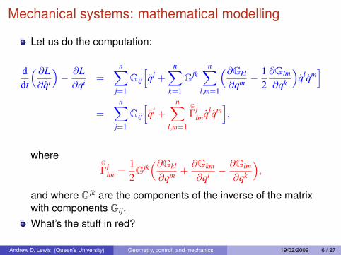
Let us do the computation:

ddt

( ∂L∂q̇i

)− ∂L∂qi =

n∑j=1

Gij

[q̈j +

n∑k=1

Gjkn∑

l,m=1

(∂Gkl

∂qm −12∂Glm

∂qk

)q̇lq̇m

]=

n∑j=1

Gij

[q̈j +

n∑l,m=1

GΓj

lmq̇lq̇m],

whereGΓj

lm =12Gjk(∂Gkl

∂qm +∂Gkm

∂ql −∂Glm

∂qk

),

and where Gjk are the components of the inverse of the matrixwith components Gij.What’s the stuff in red?



Fact: Associated to the kinetic energy metric G is a unique “affineconnection,” called the Levi-Civita connection, satisfying certainproperties.I will not say just what an affine connection is. However, incoordinates an affine connection is uniquely determined by n3

coefficients, typically denoted by Γklm, i, j, k = 1, . . . , n, called the

Christoffel symbols. For the Levi-Civita connection, these

Christoffel symbols are theGΓj

lm’s appearing on the previous slide.The differential equations

q̈j +

n∑l,m=1

GΓj

lmq̇lq̇m = 0, j = 1, . . . , n,

are the geodesic equations for the Levi-Civita connection.



Now let’s add forces. There is a rule for converting forces andmoments in the world of Newton/Euler to a single quantity which isdetermined in coordinates by components F1, . . . ,Fn. Theseappear in the Euler–Lagrange equations according to

ddt

( ∂L∂q̇i

)− ∂L∂qi = Fi, i = 1, . . . , n.

Correspondingly, the geodesic equations are modified to be

q̈j +

n∑l,m=1

GΓj

lmq̇lq̇m =

n∑k=1

GjkFk, j = 1, . . . , n.

These equations can be read: acceleration = mass−1force.



(Almost) inviolable rule: Thou shalt not separate

q̈j +

n∑l,m=1

GΓj

lmq̇lq̇m

into its summands. It is one thing, and we denote it byG∇q̇q̇.

With this notation, we can slickly write the governing equations forany mechanical system as

G∇q̇q̇ = G−1F.

Again, this is: acceleration = mass−1force.


What have we done?

We have a compact (and well-known) representation of theequations governing the motion of a mechanical system, and aprominent rôle is played by the “Levi-Civita connection associatedwith the kinetic energy metric.”So what? We already know how to write equations of motion.Question: Can we do anything interesting with the structure in ourrepresentation of the equations of motion?Answer: I think so, in control theory.


Control theory for mechanical systems

In control theory we have control over some of the external forces.Thus we write the external force F as

F = Fext +

m∑a=1

uaFa,

where Fext represents uncontrolled forces and the total controlforce is

∑ma=1 uaFa, i.e., the control force is a linear combination of

forces F1, . . . ,Fm.Assumption: F1, . . . ,Fm depend only on configuration q, and noton time or velocity q̇.


Control theory for mechanical systems

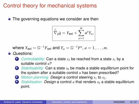
The governing equations we consider are then

G∇q̇q̇ = Yext +

m∑a=1

uaYa,

where Yext = G−1Fext and Ya = G−1Fa, a = 1, . . . ,m.Questions:

1 Controllability: Can a state x2 be reached from a state x1 by asuitable control u?

2 Stabilisability: Can a state x0 be made a stable equilibrium point forthe system after a suitable control u has been prescribed?

3 Motion planning: Design a control steering x1 to x2.4 Stabilisation: Design a control u that renders x0 a stable equilibrium

point.


(Local) controllability of mechanical systems

G∇q̇q̇ = Yext +

m∑a=1

uaYa

x0x0

big excursionsnot allowed

x0

accessibility controllability

Accessibility (does the set of points reachable from x0 have anonempty interior?) is easily decidable.Controllability (is x0 in the interior of its own reachable set?) isvery difficult to decide.



Controllability is only an interesting problem for underactuatedsystems; this excludes the “typical” robot. An example illustrateshow controllability works.



F

φ

Hovercraft system:1 Question: Is the system accessible?2 Answer: Yes (easy).3 Question: Is the system controllable?4 Answer: Yes (a little harder).



F

π2

Now suppose that the fan cannot rotate.1 Question: Is the system accessible?2 Answer: Yes (easy).3 Question: Is the system controllable?4 Answer: No, at least not locally (nontrivial).



F

τ

Change the model by adding inertia to the fan.1 Question: Is the system accessible?2 Answer: Yes (easy).3 Question: Is the system controllable?4 Answer: No, at least not locally (getting really difficult now).


The punchline

By slight alterations of the problem, a somewhat simple problemcan be made very hard. To determine the answers to some of thecontrollability questions, difficult general theorems had to beproved.The proofs of the general theorems alluded to above in a specificcontext rely in an essential way on the Levi-Civita affineconnection for the problem.So what? Can the affine connection actually be used to solve aproblem?Let’s look at the motion planning problem.


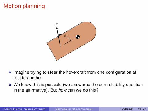
Motion planning

F

φ

Imagine trying to steer the hovercraft from one configuration atrest to another.We know this is possible (we answered the controllability questionin the affirmative). But how can we do this?


Motion planning

For the general system

G∇q̇q̇ =

m∑a=1

uaYa

(i.e., with no uncontrolled external forces) one can pose a naturalquestion: What are those vector fields whose integral curves wecan follow with an arbitrary parameterisation?This question has a very elegant answer expressed by using theaffine connection.The answer rests on some deep connections with controllability asdescribed above.In examples, the answer to this question can sometimes leaddirectly to strikingly simple motion control algorithms.


Motion planning (movies)

For the planar body:Planar body motion 1Planar body motion 2Planar body motion plan

Another flavour of motion plannerYet another flavour of motion planner

For the snakeboard:Snakeboard motion plan 1Snakeboard motion plan 2


Stabilisation using energy shaping

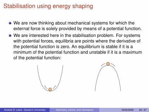
We are now thinking about mechanical systems for which theexternal force is solely provided by means of a potential function.We are interested here in the stabilisation problem. For systemswith potential forces, equilibria are points where the derivative ofthe potential function is zero. An equilibrium is stable if it is aminimum of the potential function and unstable if it is a maximumof the potential function:



Problem: Using control, can we take a system with an unstableequilibrium and make it stable by altering the potential function tohave a minimum at the desired point?For example, one can imagine the classical problem of stabilisingthe cart/pendulum system with the pendulum up:

x

θ

The input is a horizontal force applied to the cart.



Problem restatement: Can we determine the set of potentialfunctions that are achievable by using controls?If we only use control to alter the potential energy, it is possible tocompletely characterise the set of achievable potential functions.The set is often too small to be useful, e.g., for the pendulum/cartsystem, no stable potential is achievable in this way.Question: What if we allow not only the potential function tochange, but also the kinetic energy metric?Answer: The set of achievable potential functions is thenlarger, e.g., for the pendulum/cart system there is now a stablepotential achieved in this way.Caveat: To solve this problem requires solving a set of (generallyoverdetermined) nonlinear partial differential equations. . . gulp.



Nonetheless, maybe we can answer the question of when a givensystem is stabilisable using this “energy shaping” strategy.Studying the partial differential equations is complicated. Here is asimple paradigm for understanding what is going on.Problem: In Euclidean 3-space, given a vector field X, find afunction f so that grad f = X.Answer (from vector calculus): There is a solution if and only ifcurl X = 0.The condition curl X = 0 is called a compatibility condition; itplaces the appropriate restrictions on the problem data to ensurethat a solution exists.We have found the compatibility conditions for the energy shapingpartial differential equations.


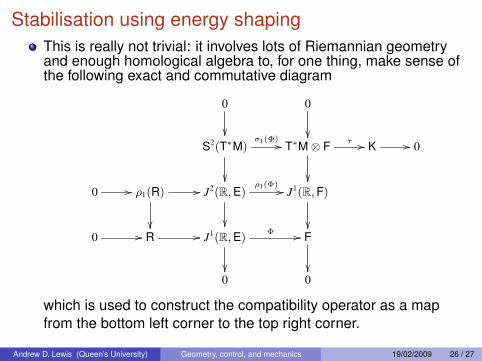
Stabilisation using energy shapingThis is really not trivial: it involves lots of Riemannian geometryand enough homological algebra to, for one thing, make sense ofthe following exact and commutative diagram

0

��

0

��S2(T∗M)

��

σ1(Φ) // T∗M ⊗ F τ //

��

K // 0

0 // ρ1(R) //

��

J2(R,E)ρ1(Φ) //

��

J1(R,F)

��0 // R // J1(R,E)

��

Φ // F

��0 0

which is used to construct the compatibility operator as a mapfrom the bottom left corner to the top right corner.


Summary

Mathematical tools can very often provide concise elegant modelsfor physical systems.Sometimes these mathematical tools can provide solutions toproblems that may not be solvable were the problems notformulated in the “right” way.


Differential geometry, control theory, and mechanicsandrew/talks/pdf/2009a.pdfDifferential geometry, control theory, and mechanics ... one can imagine the classical problem of stabilising

Documents