Diagnostika `11

International conference

Diagnostika `11held by

Department of Technologies and Measurement

Faculty of Electrical Engineering

University of West Bohemia in Pilsen

Kašperské Hory 6. - 8. September 2011

ISBN 978-80-261-0020-1Published by University of West Bohemia

Conference, of which proceedings you have just opened, is 10th in line of Diagnostics conferences, which became part of our professional life.

DIAGNOSTIKA `11follows the traditions of the previous conferences. The main aim of the conference is to interchange the experiences and to present the results of the scientific activities of participants. Objective of the conference is to create environment for creating new, and deepen current contacts of the colleagues working in the area of diagnostics of electrical appliances, electrical material science and other fields of electrotechnics.

This conference is priority event of the solved research project of Ministry of Education, Youth and Sports of Czech Republic, MSM 4977751310 – DIAGNOSTIC OF INTERACTIVE PROCESSES IN ELECTRICAL ENGINEERING, solved by our department 7th year.Conference is traditionally based on the cooperation of our department with companies working in the area of electrotechnics. This year’s opening section called „Cooperation in research”. Section is focused on presentation of R&D of following companies: BRUSH SEM s.r.o., Plzeň; COGEBI a. s., Tábor; ČEPS a.s., Praha; ETD Transformátory a. s., Plzeň; ORGREZ a.s., Brno; 1.SERVIS-ENERGO s.r.o., Plzeň; ŠKODA Electric a.s., Plzeň; VÚKI a.s., Bratislava; followed by presentation of: Petr Voda Electronics, Velké Meziříčí; Testovací technika s.r.o., Praha; Olympus, a.s., Praha; GHV Trading, s.r.o., Praha; Amedis, s.r.o., Praha; LANGROVÁ s.r.o, Plzeň.

Printed proceedings contain all accepted papers for this year conference and have got ISBN 978-80-261-0020-1. All the papers were reviewed by conference advisory board. DIAGNOSTIKA `11 is held in the attractive environment of National Park Šumava in hotel ŠUMAVA near Kašperské Hory town. I suppose, that you will find this lovely place on the “Golden creek” nice and beauty of the Šumava nature will contribute to the good atmosphere of the conference.I am hoping that all of you, participants welcomed to the conference DIAGNOSTIKA `11, will find something interesting in the conference program. Something interesting, what gain your attention, what will be new, interesting and inspiring for you in your future activities. I expect this year conference as creative and friendly as in the last years.

prof. Ing. Václav Mentlík, CSc.Conference Chair

PROGRAMME COMMITTEE

Prof. Ing. Milan Dado, PhD., ŽU ŽilinaDipl.-Phys. Tomáš Dolák, COGEBI a.s., Tábor

Doc. Ing. Karel Chmelík, VŠB, TU OstravaDoc. Ing. Eva Kučerová, CSc., ZČU Plzeň

Doc. Ing. Josef Kuchta, CSc., EVPÚ a.s., Nová DubnicaDoc. Ing. Vladislav Kvasnička, CSc., ČVUT Praha

Doc. Ing. Jaroslav Lelák, PhD., STU BratislavaDoc. Ing. Pavel Mach, CSc., ČVUT PrahaProf. Ing. Karol Marton, DrSc., TU KošiceProf. Ing. Václav Mentlík, CSc., ZČU Plzeň

Prof. Ing. Ján Michalík, Ph.D., EVPÚ a.s., Nová DubnicaPavel Novák, 1. SERVIS-ENERGO s.r.o., Plzeň

Prof. Ing. Alena Pietriková, PhD., TU KošiceDoc. Ing. Radek Polanský, Ph.D., ZČU Plzeň

Ing. František Říšský, ETD Transformátory s.r.o., PlzeňDoc. Ing. Vlastimil Skočil, CSc., ZČU Plzeň

Ing. Lumír Šašek, CSc., ETD Transformátory s.r.o., PlzeňIng. Jaromír Šilhánek, Škoda Electric a.s., Plzeň

Ing. Juraj Šmatlík, BEZ Transformátory, a.s., BratislavaDoc. Ing. Pavel Trnka, Ph.D., ZČU Plzeň

Ing. Stanislav Valenta, ORGREZ a.s. BrnoIng. Jiří Velek, ČEPS a.s., Praha

Ing. Otto Verbich, PhD., VÚKI a.s., Bratislava

CONFERENCE CHAIR

Prof. Ing. Václav Mentlík, CSc.

ORGANIZING COMMITTEE

Ing. Josef Pihera, Ph.D.Ing. Pavel Prosr, Ph.D.Ing. Robert Vik, Ph.D.

Table of contents

Laboratory Methods of Diagnostics

Diagnosis of whiskers using expert system 9 Hájek J., Žák P., Tučan M., Kudláček I.

Diagnostic of printed resinate paste 13 Hromadka K., Hamáček A., Řeboun J., Džugan T., Krpal O.

Lifetime vibration test of electronic parts 17 Hrubý J., Tureček O.

Magnetodielectric anisotropy in magnetic fluids in temperature interval from 20 °C to 80 °C

20

Marton K., Cimbala R., Kolcunová I., Kiraly J. , Tomčo L. , Timko M., Kopčanský P., Molčan, M.

A new approach in partial discharge activity: Observing of the consecutive pulses

24

Mráz P., Mentlík V., Pihera, J.

Weibull statistic in material diagnostics 28 Pihera J., Kupka L., Mráz. P, Širůček, M.

Electronic inductive probe for generator diagnostics 32 Pihera J., Švarný, J.

Change of dielectric parameters of low voltage cables within the thermal and ionizing radiation degradations

36

Procházka R., Ullman J., Hlaváček J.

Comparison of infrared spectroscopy techniques for transformer oils analysis 40 Prosr P., Polanský R.

Diagnostic methods in the quality control system in the production of plastic materials for direct food contact

44

Samsonek J., Vaculík L.

Program for prediction of the rest lifetime of rotary machine insulating system 48 Trnka P., Svoboda M., Souček J.

Detecting Non-Homogenity of Electrically Conductive Adhesives 53 Tučan M., Žák P., Urbánek J.

5

On-Site Testing of Electrical Appliances

Measurement of railway traction transformer using by SFRA method - part 1 57 Brandt, M., Michalík, J., Kuchta, J.

Measurement and analysis of railway traction transformer using by SFRA method – part 2

61

Brandt, M., Seewald, R., Sedlák, J., Faktorová, D.

Evaluation circuit for IDE sensor structures 65 Freisleben J., Hamáček A., Řeboun J.

Use of Internet as an instrument for control of measurement instruments in materials diagnostic

69

Frk M., Rozsívalová Z.

Dielectric absorption of insulating system generators in operation 73 Hájková L., Petr J., Hájek J.

Noise source identification using sound intensity measurement 77 Klasna J.

Fast controlled transfers process analysis of 6 kV switchgear in NPP 81 Mareček O., Kaška M.

Energy audit and revisions of power equipments 85 Šebök M., Gutten M., Kučera M., Korenčiak D.

Requirements for assessment of LOCA cables VUKI in deliveries for the Mochovce NPP

89

Verbich O., Sulová J., Valach R.

Electrical Insulation Properties and Structural Changes

Epoxy-POSS nanocomposite for electro-insulating materials 93 Boček J., Mentlík V., Trnka P.

Investigation and Diagnostic of Magnetic Control of Cryogenic Heat Pipes 97 Cingroš F., Kuba J.

Moisture within transformer insulation system 101 Dončuk J., Mentlík V.

Radiation Ageing of Flame Retardant XLPE Cables 105 Ďurman V., Lelák J.

Life Cycle Assessment of photovoltaic system in intelligent buildings 109 Hájek J., Žák P., Kudláček I.

6

Dielectric Properties of epoxy resins with TiO2 nanofillers 113 Klampár M., Liedermann K.

Design and verification of properties of some components for magnetic refrigeration near room temperature

117

Kuba J., Hron T.

Insulating materials and cryogenic temperatures 121 Kučerová E., Matějka F., Šebík P., Krpal O.

Study on the Effect of Addition of Spherical Silver Nanoparticles into Electrically Conductive Adhesives

126

Mach, P.

Partial discharges and breakdown voltage diagnostics during thermal aging of insulating materials

130

Pihera J., Mráz P., Haller R., Mentlík V.

Diagnostic system for cable insulation materials 136 Pinkerová, M., Mentlík, V.

Dielectric properties of a composite based on epoxy resin 141 Polsterová H.

Influence of Thermal degradation on Electrical Parameters of Winding Insulating System of Power Transformers

144

Širůček M., Trnka P., Paslavský B.

Other Diagnostic Methods

Software for stator bars design, 3D models of stator bars and 3D models of jigs 148 Bezděkovský J., Krupauer P.

Issues of flicker noise measurements on power semiconductor devices 152 Hájek J., Papež V.

The distribution of voltage on the inductor during surge testing (RSO) 156 J. Lábadi, Z. Křelovec

Seebeck effect of ECA 160 Koblížek V.

Diagnostics of electrical equipment as a tool for risk management measures 164 Kopča M., Váry M.

A new ERM winding impregnation quality assessment method 167 Kotlárik B., Vaňková R., Filová Z.

7

Less common used methods of DOE 173 Motyčka M., Tůmová O.

Analysis of induction machine reliability by means of FRA method 177 Poliak, J., Gutten, M.

Relation of electro insulating fluids to the environment 181 Trnka P., Souček J., Svoboda M.

Is FMEA a risk? 185 Tůmová O.

What will be the evolution of International System of Units after the year 2011?

189

Tůmová O., Kupka L.

Estimation of Weibull Distribution Parameters for Reliability 193 Žák P., Tučan M., Kudláček I.

Contribution to the study of lead-free technology in terms of LCA 198 Žák P., Tučan M., Kudláček I.

8

Diagnosis of whiskers using expert system Hájek J., Žák P., Tučan M., Kudláček I. – FEE CTU in Prague Abstract Many studies show that if an organization used to solve fundamental problems of analytical tools, their solution is more efficient. Therefore, these instruments particularly in recent years become very topical. Expert systems can be used to design solutions to the situation on the basis of observations and hypotheses, where there is no solution using traditional algorithms. The condition for correct functioning of an expert system, is entering the correct terms by human expert. In this paper, are studied in detail the possibility of using expert systems in managing risks associated with the formation of whiskers in industrial systems. Tin whiskers are electrically conductive thin single crystal structure of spontaneously growing out of metal surfaces - often tin, cadmium and zinc. Whiskers pose a serious risk to the reliability of electrical equipment because of their conditions are not yet fully specified. That is why there is another use of expert systems. Motivation

Eutectic tin-lead (SnPb) solder has been during long time the primary choice for assembling electronics due to technological properties – especially low melting point. However, concern over lead’s and its toxicity have resulted into restriction of its use – RoHS directive in the EU and similar directives in other countries. Although lead-free electronics is environmentally friendly there are some difficulties with their long-term stability – especially tin whiskers. Whisker failure modes In practice, the whiskers can cause particular the following failure modes:

1. Permanent electrical short circuit – a phenomenon can occur in electrical circuits with high impedance and low voltage (current flow does not cause melting and breaking of the whisker).

2. Temporary short circuit – during the short circuit electrical circuit´s parameters allow to achieve the current that causes melting and breaking of whiskers. Short-circuit current depends only on the parameters of the circuit and overcurrent protection.

3. Electric Arc – Electrical circuit parameters allows the passage of current, which causes evaporation of the tin whisker phenomenon after a short circuit, and subsequent metal vapor arc (MVA). Evaporation of the whisker can cause an arc, which can pass current up to hundreds of amperes. This electrical arc is capable of maintaining for relatively long period of time, which is mainly caused by a release time of overcurrent protection and/or external destructive influences of peripheral components (particularly wire mechanical resistance). In this case, even the fire of equipment can not be excluded. The extraordinary dangers of the phenomenon represent for electrical equipment operated at reduced atmospheric pressure, where conditions for maintaining the arc is considerably more favorable.

4. Whiskers fragments - whiskers loosed from tin layer can move in the device uncontrollably so that they can cause random electrical shorts or problems for MEMS.

All of above mentioned events represent direct threat to the reliability of the device simply because the detection of whiskers is not simple due to their small size so it requires high-quality optical microscope and also some experience. It is indisputable that in many

9

cases the so-called unexplained electrical failures can be attributed to in a certain portion to tin whiskers as the primary cause. In addition, each of these phenomena leads to the destruction.

Whisker mitigation methods Long-term resistance of tin whiskers was observed on the deposited layer of eutectic

solder Sn60Pb. You can assume that the admixture of lead was just a kind of retarder to minimize mechanical stress in the layer.

The effect of metal underlayer as a whisker inhibitor was also studied in this research. The presence of electrodeposited metal interlayer had only limited influence. In some cases, the copper interlayer was used on the base material of tin bronze. This layer has been proved as a counterproductive, contrary this layer was promoting growth of tin whiskers. Nickel (Ni) interlayer has very limited effectiveness, layer up to 2 ÷ 3µm are proving to be very porous so they do not reduce the possibility of tin whiskers occurrence. It is possible that a further increase in the thickness of the interlayer of nickel could lead to reducing tin whiskers occurrence.

Fig. 1: Flowchart diagram of most used mitigation practices

Whisker risk mitigation in existing installation

While it is possible to mitigate the risk presented by whiskers by carefully choosing technologies and materials, often we do not have such a luxury available. Especially with already existing devices and installations, it is often impossible to replace relevant parts. In such case it is recommended to realize the risk presented by whiskers and to act accordingly. First step is an optical check, which can be used as part of standard maintenance procedures or as an emergency check in case short-circuits of unknown origins start to appear in the system.

Whiskermitigation onconnectors

Are any connectorswith pure tin finish

used?

No designchange

Can we useother

finish?

Process shiftto non-puretin finish.

Can we usenickel

underlayer?

Designchange

Can we usethick layer

of tin?

Can we useannealing?

Designrevisionneeded.

NO

YES

YES NO YES

NO

NONO YES

YES

10

While whiskers are very thin and thus hard to see using naked eye, there are two basic methods that can present them better. If the whiskers are long enough, they can be seen if shown against a bright background, such as planar light source. In case this method cannot be used, there is a chance of detecting them using bright light source and changing the angle – under right conditions, even small whiskers can sparkle brilliantly and thus announce their presence.

Use of small handheld USB microscope is recommended, as it can show more details than an eye. It also usually comes with its own lighting, so again it allows for changes of angle and searching for brightly sparkling whiskers. In case whiskers are found in the installation and it is impossible to replace parts infested by whiskers, it is possible to remove them. Utmost care must be paid to the operation, though, so that broken whiskers do not fall inside the device. If given part can be removed for cleaning, it should be. Soft carbon brushes are usually enough to remove whiskers, and it is advisable to use a vacuum cleaner to remove all broken parts of whiskers. If the part cannot be removed, the vacuum cleaner shall be used in all cases and its intake shall be placed as close to the brush as possible to catch all breakaway whiskers. Expert systems in practice

Expert systems have many practical uses. One of more possible application could be using for estimation probability occurrence of whiskers dependent on environmental conditions. It could be application of conditions described above. Expert system is decision making mechanism based on assumptions and observations. The assumption is true at observation with some probability. The difference between expert system and any other computer program is that expert system has knowledge outside a program source. Program is done only result of observation. Expert system can work with uncertainty (e.g.: guess yes, yes, don’t know, guess no, no) not only with binary decision (yes, no). It can also work with rules which are against self. Weakness of expert systems is critical dependency of accuracy knowledge base. In other words, how exactly the person who inputting knowledge data (human expert) can define his knowledge, that means decision criteria. An example how could look a diagram of knowledge base for decision of solution whisker mitigation is implied on Fig. 2. It was created from flowchart diagram on Fig. 1.

Fig. 2: Knowledge diagram

11

Conclusions This article attempted to provide a brief overview of both current methods of whisker

mitigation and possibilites to use expert systems for this purpose. Whiskers represent reliability risk for electronic components and devices. Risk

assessment is needed in order to try to avoid their growth. Expert systems present one possibility how to make fast decision which solution is the best in a current situation. Use of expert systems allows the user to avoid the need of consulting specialists constantly. Unfortunately, they do not present an absolute guaranteee of avoiding the risk. They should, however, give an additional tool for production planning and problem solving.

In case of major problems caused by this phenomenon, though, it is usually better to contact specialised research institutions and employ their knowledge and laboratory background. This is accented if any large-scale whisker infestation appears even though all the above mentioned mitigation steps and procedures were taken. References 1. Directive 2002/95/EC, OJ L 37, 13.2.2003, p. 19–23 of 27.1.2003. 2. ČSN EN 60068-2-82. Environmental testing - Part 2-82: Tests - Test Tx: Whisker test

methods for electronic and electric components. 1.2.2008. 32 s. 3. Žák, P. - Kudláček, I.: Tin Whiskers - Reliability Risk For Electronic Equipment. In

Umwelteinflüsse erfassen, simulieren, bewerten. Pfinztal (Berghausen): Gesellschaft für Umweltsimulation e.V., 2009, p. 239-251. ISBN 978-3-9810472-7-1.

Authors Bc. Jan Hájek, Ing. Pavel Žák, Ing. Marek Tučan, Doc. Ing. Ivan Kudláček, CSc.; Department of Electrotechnology, Faculty of Electrical Engineering, Czech Technical University in Prague; Technicka 2, 16627 Prague 6, e-mail: [email protected], [email protected], [email protected], [email protected].

12

Diagnostic of printed resinate paste Hromadka K., Hamáček A., Řeboun J., Džugan T., Krpal O. – FEE UWB in Pilsen Abstract This paper deals with the diagnostic of conductive patterns which are made by silver resinate paste on a ceramic substrate. The aim of this paper is to compare printed patterns quality by various printing parameters of resinate paste and select an optimum printing method. The quality of the final pattern is dependent on many printing machine parameters like: squeegee speed, squeegee pressure or screen snap off. Several sets of samples were investigated in order to determine the appropriate printing method. Each set is different in various patterns preparation parameters. The laser confocal microscope LEXT OLS3000 from Olympus was used for visual checking and measurements. Next objective was to measure electrical properties of printed patterns. The resistance of the conductive paths was measured using Keithley multimeter, the insulation resistance between nearby conductive patterns (IDE structure) was measured using Keithley electrometer. Introduction

Screen printing is one of the most common methods for additive creating of conductive patterns [1]. The main goal is to create fine and thin patterns. Thick film pastes usually used in screen printing contains particles of precious metals of a certain size (usually tens of microns) [4]. Precision metals normally used for the thick film paste are Ag, Au, Pt. The screen size must be adapted to these particles. The printed patterns dimensions are limited by a maximal size of paste particles. Disadvantages of standard thick film paste can be eliminated using resinate paste. The resinate paste consists of an organic material which contains a small amount of metal atoms in its molecules. The main advantage of creating patterns by the resinate paste is fine pattern printing with the thickness below 1 µm. [2,3]

Test samples description

The test board design is proposed for the advanced thin film screen printing experiments on the ceramic substrate with dimension of 4”x4”. The geometrical and electrical measurements, adhesion, soldering, bonding and gluing tests can be made on the designed test board. Except this, the board includes the basic function elements like: Horizontal and vertical lines with sharp 90° corners for edge resolution optical

investigation. The ratio of gaps / lines is 1:1. The width of lines / gaps is 25, 50, 75, 100, 200 µm. (see Fig. 1)

Conductive meanders with the active area 4 x 4 mm. The width of lines is 50, 100, 200 µm. The meanders are situated in vertical and horizontal direction of printing. (see Fig. 2)

Interdigital electrodes (IDE) with gap / line ratio 1:1. The active area of IDE is 4 x 4 mm. The lines / gaps width is 50, 100 and 200 µm. The IDE are situated in vertical and horizontal direction of printing. (see Fig. 3)

Lines with constant number of squares are placed in area 4. The number of squares is 7500. The width of lines is 25, 50, 100, and 200 µm. (see Fig. 4)

13

Fig. 1: Horizontal and vertical lines Fig. 2: Conductive meander

with sharp 90° corners with different lines / gaps widths

Fig. 3: Interdigital electrodes with different line / gap widths

Fig. 4: Lines with constant number of squares Samples preparation

The test patterns were printed by a screen printing machine (Tab. 1) using silver resinate paste on the ceramic substrate. The different parameters of the printing were used. The selected parameters of the screen printing machine are shown in Tab. 2.

Table 1: Screen printing process description Printing machine: DEK Galaxy Screen type: 325/24/45 Ambient temperature: 24,7 °C Humidity: 30 %RH Clean room level: 100000

Table 2: Printing parameters

Squeegee pressure (kg): 2 – 8 Snap off (mm): 1 – 2 Squeegee speed (mm / s): 10 – 50

At least 3 prints were printed for each combination of set parameters. The third print

represents steady process of printing and next prints show similar results. The third sets of print were used for drying, firing and testing. The printed test boards were dried for at 90 °C for 15 minutes and fired at 850 °C (peak) for 7 - 10 minutes with a total time of the firing cycle at least 60 minutes.

14

Print diagnostic The laser confocal microscope LEXT OLS3000 from Olympus was used for visual

checking and measurements. Pictures were scanned with the magnification of 120 times in the colour mode. The best and the worst results before and after firing are shown in Fig. 5 and Fig. 6.

The investigation shows that the higher squeegee pressure causes wider printing lines but the minimal pressure level must be at least 2 kg. The higher speed and higher snap off cause narrower printed lines.

Fig. 5: The worst and the best print before firing (lines / gaps width 100 µm)

Fig. 6: The worst and the best print after firing (lines / gaps width 100 µm)

The Keithley 2700 multimeter was used for the electrical measuring of the conductive

meanders and lines with constant number of squares. Keithley 6517A electrometer / high resistance meter was used for electrical measuring of IDE. Conductive paths are short-circuited for the width of the paths 50 µm. Also IDE are short-circuited for the width 100 µm. These conductive patterns were not measured. The average values are shown in Tab. 3.

Table 3: Average values of conductive patterns

IDE Conductive meanders Lines with constant

number of 7500 squares

Line width [µm]

200 200 200 200 100 100 200 100

Orientation I P I P I P I I R [Ω] 1,13 GΩ 1,15 GΩ 22,7 25.9 89,6 69.3 126 202

I...lines in the direction of printing P...lines perpendicular to the direction of printing

15

Conclusion The optical and electrical testing shows that increasing of squeegee pressure has

negative impact on the printed width of lines. The higher pressure causes wider printed lines. The minimal level of the squeegee pressure is 2 kg. Lower pressures cause that the printed lines are intermitted. The increasing of squeegee speed has positive impact on the printed width of lines. The higher speed causes narrower printed lines. Increasing of the snap off has slightly positive impact on the printed width of lines. The higher snap off causes narrower printed lines. The average insulation resistance of interdigital electrodes with 200 µm gaps width is 1,1 GΩ. The average resistances of conductive meanders with 200 µm lines width are 25 Ω and 80 Ω for 100 µm lines width. The average resistances of lines with 7500 squares are 126 Ω for 200 µm lines width and 202 Ω for 100 µm lines width. Next work in this area will be focused on fine line printing of conductive patterns with lines width bellow 100 µm. Acknowledgement

This paper was supported by the project EURIPIDES INTEX OE10015: “Intelligent Sensing and Communication Textile.” References 1. Elektrotechnologie: materiály, technologie a výroba v elektronice a elektrotechnice. 3.,

rozš. vyd. Praha : BEN - technická literatura, 2004. 299 s. 2. KOŘÍNEK, Ota; KOMÁREK, Antonín; LUTTERER, Vladimír. Sítotisk a serigrafie.

Praha : Ota Kořínek, 1991. 136 s. 3. KOSLOFF, Albert. Screen printing techniques. Pennsylvania State University : Signs of

the Times Pub. Co., 1981. 342 s. 4. Heraeus [online]. 2011 [cit. 2011-06-13]. Dostupné z WWW:

<http://www.heraeus.com/en/home/default.html>. Authors Ing. Karel Hromadka, Doc. Ing. Aleš Hamáček, Ph.D., Ing. Jan Řeboun, Ing. Tomáš Džugan, Ing. Ondřej Krpal; Department of Technologies and Measurement, Faculty of Electrical Engineering, University of West Bohemia in Pilsen; Univerzitní 8, 30614 Pilsen; e-mail: [email protected], [email protected], [email protected], [email protected], [email protected].

16

Lifetime vibration test of electronic parts

Hrubý J., Tureček O. – FEE UWB in Pilsen

Abstract This paper deals with the lifetime vibration test preparation of THT electronic parts. The specification

of this test comes from Czech technical standards and from customer’s requirements. The swept

sinusoidal signal was used for this test instead of testing only on each resonant frequency (sinusoidal

dwell vibration test on resonant frequencies). Frequency correction was made according to the

measured data.

Introduction

The vibration tests are generally used for determination of mechanical resistance of the

tested samples and they should simulate dynamical mechanical stresses during the regular use

and during the transport. This testing method was created for testing of new produced

electronic parts. The specification of the vibration test comes from recommendation of Czech

technical standards (ČSN EN 60068 - 2 - 6 [1] and ČSN EN 60068 - 2 – 47 [2]) and from

customer’s requirements. The customer sets the following test conditions: number of

dynamical stress cycle, temperature, humidity, maximum level of magnetic field interference,

the position of the samples (in which axes inflicts the vibrations the sample) and the kind of

testing signal (vibrations amplitude and frequency range).

Description of testing method

Testing samples were mounted on the shaker with help of the aluminium fixture. This

material is better than steel, because the internal mechanical damping is higher than in the

steel and the propagation speed of the vibration is slower. These attributes reduce the

formation of self-oscillation of the fixture. The maximum size of the fixture must be smaller

than the quarter of minimum wavelength of the vibrations.

maxmax 44

;f

vll

f

v

(1)

It is very important to consider the geometrical structure of the fixture (it must be

sufficiently tough) and the placement of the accelerometer (for vibration measurement and

control).

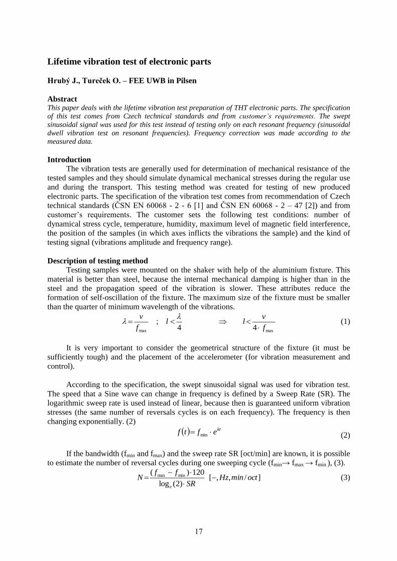
According to the specification, the swept sinusoidal signal was used for vibration test.

The speed that a Sine wave can change in frequency is defined by a Sweep Rate (SR). The

logarithmic sweep rate is used instead of linear, because then is guaranteed uniform vibration

stresses (the same number of reversals cycles is on each frequency). The frequency is then

changing exponentially. (2)

kteftf min (2)

If the bandwidth (fmin and fmax) and the sweep rate SR [oct/min] are known, it is possible

to estimate the number of reversal cycles during one sweeping cycle (fmin→ fmax → fmin ), (3).

]/,,[)2(log

120)( minmax octminHzSR

ffN

e

(3)

17

2

)sin(

2)sin(

minmax

minmax

Ttwhereetfata

Ttwhereetfata

kt

kt

(4)

Where T is period of sweeping cycle and constant k corresponds to equation (1). On the

basis of previous equation, the audio file in *.wav format was generated with following

parameters: length of 11 min 18 s with sweep rate of 1 Oct./min and bandwidth from 10 Hz to

500 Hz (up and down).

Measurement

After fitting the fixture with testing samples on the shaker, the frequency response must

be checked, whether the amplitudes of acceleration are constant as the electrical control

signal. The curve shape of the acceleration can be affected by the own frequency

characteristic of the shaker, free oscillation of the fixture or by the frequency characteristic of

the amplifier. The frequency characteristic of acceleration in third octave bands is shown in

Fig. 1.

0

5

10

15

20

25

30

35

8,0

10,0

12,5

16,0

20,0

25,0

31,5

40,0

50,0

63,0

80,0

100,0

125,0

160,0

200,0

250,0

315,0

400,0

500,0

630,0

f [Hz]

a(f

) [m

s-2]

Fig. 1: Acceleration dependence on frequency before equalization

The equalization of control signal (*.wav file) was accomplished according to

characteristic in Fig. 1. The final frequency characteristic is shown in Fig. 2 and the

equalization was made with help of software parametric equalizer.

18

0

5

10

15

20

25

30

35

8,0

10,0

12,5

16,0

20,0

25,0

31,5

40,0

50,0

63,0

80,0

100,0

125,0

160,0

200,0

250,0

315,0

400,0

500,0

630,0

f [Hz]

a(f

) [m

s-2]

Fig. 2: Acceleration dependence on frequency after equalization

Conclusions

The main goal of this test method is to simulate the expected dynamical vibration

stresses of the electronic parts considering the expected lifetime period. The electrical

parameters of new produced parts were also tested.

References

1. ČSN EN 60068-2-6: Zkoušení vlivu prostředí – Část 2-6: Zkoušky – Zkouška Fc:

Vibrace (sinusové)., Praha: Český normalizační institut, 2008.

2. ČSN EN 60068-2-47: Zkoušení vlivu prostředí – Část 2-47-: Zkoušky – Upevnění vzorků

pro zkoušky vibracemi, nárazy a obdobné dynamické zkoušky., Praha: Český

normalizační institut, 2006.

Authors Ing. Jan Hrubý, Ing., Oldřich Tureček, Ph.D.; Department of Technologies and Measurement, Faculty

of Electrical Engineering, University of West Bohemia in Pilsen; Univerzitní 26, 306 14 Pilsen;

e-mail: [email protected], [email protected].

19

Magnetodielectric anisotropy in magnetic fluids in temperature interval from 20 °C to 80 °C Marton K., Cimbala R., Kolcunová I., Kiraly J. – FEEI TU in Košice; Tomčo L. – FA TU in Košice; Timko M., Kopčanský P., Molčan, M. – IEP SAS Košice AbstractSubstitution of transformer oil as insulator medium by magnetic fluid in transformers requires observation of electric properties of magnetic fluids at temperatures higher than 20 °C. That´s why important physical quantities were measured at temperature in interval from 20 °C to 80 °C. The magnetodielectric anisotropy was studied at the same temperature region. Two important quantities have been measured: specific electric conductivity and dielectric breakdown strength of magnetic fluids at volume concentrations from 0,185 % to 2 %. So the behavior of magnetic fluids as insulator medium could be observed at working conditions of transformers. Introduction

The application of magnetic fluids as insulator medium in transformers of high voltage has not been done sufficiently deep so far. The structure of magnetic fluids themselves shows that magnetic fluids are complex material consisting of three components: nonpolar component – inhibited transformer oil as carrier liquid, polar component – oleic acid as surfactant and solid magnetite nanoparticles of average diameter 10 nm. The still completed measurements of electric properties have showed fair-sized differences of observed fluid particularly when observed medium is placed into combined electric and magnetic fields at two different orientations of used fields (E∥H, E⊥H).

The goal of this work was observation of magnetodielecric anisotropy of both dielectric breakdown strength (Eb) and specific electric conductivity [1] of magnetic fluids based on transformer oil and observation temperature dependences of important quantities characterizing electric properties of magnetic fluids. The experiments have proved the presence of electrophoretic conductivity in magnetic fluids, too.

TheoryComplex physico-chemical character of the magnetic fluids requires investigation of

their properties:• in DC and AC electric fields,• in weak (below 106 V.m-1) and strong electric fields (above 107 V.m-1),• in "clean" - nonpolar insulating liquids, in polar liquids with surfactant and in

pigmented liquids by colloidal nanoparticles.Based on the elementary Ohm's law in differential form di=γ EdE , after a detailed

analysis we get this equation:

γ=n0 q bi=n0 q

2 υ6 kT

exp−W a

kT (1)

where bi is the ion mobility, that is also exponentially dependent on temperature T and it can be expressed as:

b i=υi

E=

q2υ

6kTexp

−W a

kT (2)

where δ is the distance of potential holes, υ is the frequency (eg. 1012-1013 s-1) and Wa is the activation energy.

20

The coefficient bi in mineral oils, when weak electric fields are applied, reaches value of 10-8 m2.s-1.V-1 and in strong fields it increases to 10-7 m2.s-1.V-1 (mobility of negatively charged ions). When DC field (voltage) is applied on a magnetic fluid containing nanometer sized particles of ferrites then it is expected that electrophoretic conductivity occurs in the inter-electrode space, which is defined as follows:

γ k=ε2 rnk

6 π η(3)

where ξ is the electrokinetic potential, η is the dynamic viscosity, ε is the electric permittivity and r is the particle radius. Electrical conductivity of liquid insulating material is often associated with the viscosity η of the liquid, that is dependent on temperature, which can be expressed as:

η=6 kTγ3 υ

exp W a

kT (4)

The equation (4) is a part of Walden's law that is applicable on nonpolar (or weakly-polar) liquid insulators in the form:

γ η=const. (5)Relationship between the specific electrical conductivity and electrical stability can be

found from modelling of heat transition, when we come out from the model of a dielectric (insulator) placed between two plane parallel electrodes. After creation of differential equations that corresponds to balance state of energy, we get the equation [3]:

−λdTdz

∣zdz λdTdz

∣z =γ E2 dz (6)

where λ is the coefficient of thermal conductivity of dielectric material (oil), γ is the equivalent conductivity of liquid media. The maximum intensity of electric field at a generated temperature can be reached by another solution of the differential equation (6).

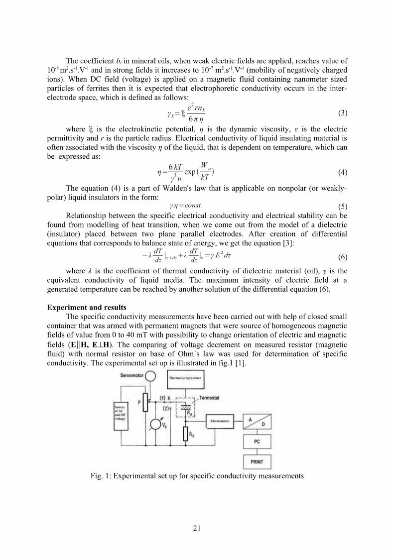
Experiment and results

The specific conductivity measurements have been carried out with help of closed small container that was armed with permanent magnets that were source of homogeneous magnetic fields of value from 0 to 40 mT with possibility to change orientation of electric and magnetic fields (E∥H, E⊥H). The comparing of voltage decrement on measured resistor (magnetic fluid) with normal resistor on base of Ohm´s law was used for determination of specific conductivity. The experimental set up is illustrated in fig.1 [1].

Fig. 1: Experimental set up for specific conductivity measurements

21

The experiments have been carried out with magnetic fluids of volume concentration of magnetite particles from 0,185 % to 2 % at DC voltage from 200 V to 1000 V. The course of dependencies γ = f(T) with U as parameter showed the validity of equation (1). The magnetodielectric anisotropy was more distinct at higher values of voltage.

Fig. 2: The dependencies of specific conductivity on temperature at voltage of 200 V The measurements of dielectric breakdown strength, i.e. dielectric stability of magnetic

fluids were carried out on the base on the STN norm. The sample of magnetic fluids was placed into small container that was armed by Rogowski´s electrodes and permanent magnets (NdFeB). Magnetic fluids temperature was controlled by ultra thermostat.

Fig. 3: Experimental set up for dielectric breakdown strength measurements [4]

Electric field intensities were higher than 107 V.m-1, i.e. experiments were carried out in strong electric field. The course of dependencies in fig.4 corresponds to the same dependency for pure mineral oil that contains small amount of water (0,02 %) at low temperature. Water at higher temperature changes from state of emulsion solution to molecular state and so dielectric breakdown strength reaches lower values. This decrease is caused by increasing of magnetic fluid conductivity. The observed maximum of dependency at perpendicular orientation of magnetic and electric fields shifts to lower temperatures.

22

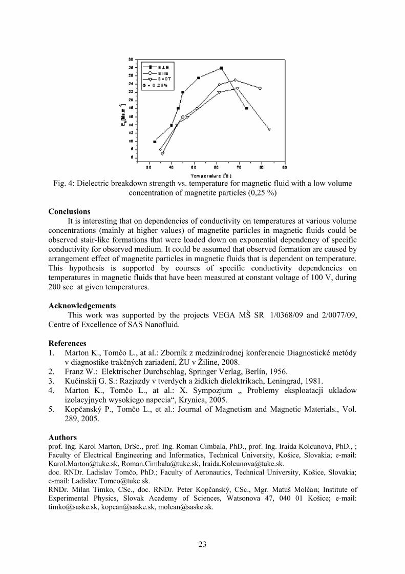
Fig. 4: Dielectric breakdown strength vs. temperature for magnetic fluid with a low volume concentration of magnetite particles (0,25 %)

ConclusionsIt is interesting that on dependencies of conductivity on temperatures at various volume

concentrations (mainly at higher values) of magnetite particles in magnetic fluids could be observed stair-like formations that were loaded down on exponential dependency of specific conductivity for observed medium. It could be assumed that observed formation are caused by arrangement effect of magnetite particles in magnetic fluids that is dependent on temperature. This hypothesis is supported by courses of specific conductivity dependencies on temperatures in magnetic fluids that have been measured at constant voltage of 100 V, during 200 sec at given temperatures. Acknowledgements

This work was supported by the projects VEGA MŠ SR 1/0368/09 and 2/0077/09, Centre of Excellence of SAS Nanofluid. References1. Marton K., Tomčo L., at al.: Zborník z medzinárodnej konferencie Diagnostické metódy

v diagnostike trakčných zariadení, ŽU v Žiline, 2008.2. Franz W.: Elektrischer Durchschlag, Springer Verlag, Berlín, 1956.3. Kučinskij G. S.: Razjazdy v tverdych a židkich dielektrikach, Leningrad, 1981.4. Marton K., Tomčo L., at al.: X. Sympozjum „ Problemy eksploatacji ukladow

izolacyjnych wysokiego napecia“, Krynica, 2005.5. Kopčanský P., Tomčo L., et al.: Journal of Magnetism and Magnetic Materials., Vol.

289, 2005. Authorsprof. Ing. Karol Marton, DrSc., prof. Ing. Roman Cimbala, PhD., prof. Ing. Iraida Kolcunová, PhD., ; Faculty of Electrical Engineering and Informatics, Technical University, Košice, Slovakia; e-mail: [email protected], [email protected], [email protected]. RNDr. Ladislav Tomčo, PhD.; Faculty of Aeronautics, Technical University, Košice, Slovakia; e-mail: [email protected]. Milan Timko, CSc., doc. RNDr. Peter Kopčanský, CSc., Mgr. Matúš Molčan; Institute of Experimental Physics, Slovak Academy of Sciences, Watsonova 47, 040 01 Košice; e-mail: [email protected], [email protected], [email protected].

23

A new approach in partial discharge activity: Observing of the consecutive

pulses

Mráz P., Mentlík V., Pihera, J. – FEE UWB in Pilsen

Abstract This paper describes a new view on partial discharge (PD) activity phenomenon. PD activity is

attended with a formation of the local space charge, especially in solid dielectrics like composite

insulating materials of rotating machines. It caused the change of the local field near the defect and

subsequent origin of PD activity. It means that the inception conditions for the consecutive discharge

were changed. A new diagnostic method called pulse sequence analysis considers the issue of

consecutive pulses and offer better view into the problematic of PD activity. The paper describes the

main principles of this method and the first experience with it.

Introduction

Nowadays the consumption of electrical energy increases all around the world. Because

of that it is very important to focus to the machines, which produces this kind of energy.

There are a lot of parameters which should be study and improve e.g. efficiency and

reliability. Diagnostic of electrical rotating (motors, generators) and non-rotating

(transformers, chokes) machines is well-known and using tool for determining the machine

state and condition. It is necessary to aim effort to the reliability these machines, which can

cause enormous financial losses and big problems in infrastructure function of state,

respectively all society if they stop working.

One of the very important diagnostic parameter is partial discharge (PD) activity

detection in insulating system of machines. Of course also in electro technical field the well-

known rule hold true - the system is reliable only as much as its weakest part. In case of

electrical rotating machines was find out that the weakest segment (in the reliability point of

view) is insulating system of stator. Question is why even we should deal with partial

discharge activity. History of PD investigation goes up to 1930s. However the important turn

arose at 1960s, when the fundamental change came in the insulating system of rotating

machines. Up to these days the compact tar insulating systems were used. But of course they

had several disadvantages e.g. moistening and low resistance to the higher temperatures.

When the new composite thermoset isolations based on epoxy polyesters come, the electrical

strength arises. However the new problem occurred. This problem is just partial discharge

activity. In case of tar mixtures the stator bars were filled perfectly. So the system was

perfectly compact and homogenous. Composite insulations are lighter and have higher

electrical strength, but despite modern technological processes it is almost impossible to

produce them without any air voids or nonuniformities in the structure of the material. These

cavities are source of partial discharges, which has negative impact on the lifetime of

insulating materials. The main problem is caused by the slot discharges, up to that times

unknown problem.

Detection and evaluation of PD activity helps during the designing new segments of

electrical machines (primarily insulating systems), but also it is suitable diagnostic tool

helping to determinate current state of the machine. Thanks to the PD detection it is possible

to prevent destructive changes in the machines and plan lay-offs and regular maintenance of

the machines.

24

Partial Discharge activity evaluation

Nowadays there is no problem with detection of the PD activity. Measuring apparatus

are high sophisticated and sensitive and they are able to relatively good and precisely record

partial discharges. However current problem is evaluation of PD, in another words problem is

the right physically and logical interpretation of measured results.

Today there are evaluating some accumulation data captured during the long-term

measurements. These data have usual big statistical scatter. For example the values of

apparent charge fluctuate from tens to hundreds of pico-coulombs (pC). To evaluate these

data there are usually made some statistical operations, when the part of the measured data is

often left out – data are declared like statistical remote or they are deleted like the mistake of

measurement.

Because of this the very important information can be lost and the behaviour of partial

discharges is not able to be described in the right way and with sufficient quality. The pulse

sequence analysis offers the better view into the mechanism and influence of consecutive

pulses and tries to solve the problem mention above.

Nature of pulse sequence analysis

Because of the local overstress in the specific location of insulation, the partial

discharges occur. In this location arise an increasing accumulation of electrical charge. It

causes the change of the local field around the place. Because of that it is very probable that

just this location has a big influence to the follow discharge. The local space charge of the

previous pulse, which remains close to this location, influences the inception conditions of

consecutive pulses. Due to that it is not possible to evaluate only single pulses independently,

but it is necessary to take advance its mutual correlation.

Method pulse sequence analysis (PSA) evaluates the changes of the local field and its

space charge. Conventional parameters for evaluation of PD activity are apparent charge q,

count of pulses n and the range of phase angles between 0° and 360°. The well-known Φ-q

and Φ-q-n diagrams are done. Against this, PSA method operates with the voltage change,

which occurs between the current and next discharge pulse, because the corresponding change

of the local electric field at the discharge site determines the ignition of the next pulse.

First experience with PSA method

There were done several measurements on the basic partial discharge arrangements to

see the behaviour of the PSA method. Test arrangements used for experimental measurement

of partial discharges are shown in table 1.

Table 1: Test arrangements

Corona

Needle plane with

insulating material

Gliding discharge

Corona

Needle-sphere

Internal discharge

25

Figure 1 shows the PSA diagram of internal partial discharges. There are obvious strong

symmetrical triangles in the 1st and 3

rd quadrant. Needle-sphere arrangements shown in figure

2 obviously different PSA spread. In the 3rd

quadrant is square which turns to the triangle and

in the 1st quadrant there is virtual triangle with two cathetus and no hypotenuse. Its specific

shape of PSA diagram, which can be seen in the figure 3 has also corona represented by

needle-insulating plane arrangement. It is typical with the square in the 1st quadrant and the

triangle in the 3rd

quadrant. Finally figure 4 describes the PSA diagram for gliding discharges.

There are two symmetrical shapes according to the axis y and also two cluster of points on the

axis x.

Fig. 1: Internal partial discharges (20 kV)

Fig. 2: Needle-sphere arrangement (5 kV)

Fig. 3: Needle-insulating plane arrangement (8,87 kV)

Fig. 4: Gliding discharge arrangement (9,31 kV)

26

Conclusions

This paper describes a view on a new partial discharge evaluation method. The aim of

the paper was not to deeply explain the nature and principles of the pulse sequence analysis,

which deals with consecutive pulses, but only evoke the discussion about this relatively new

method and shown its basic principles and first experiences with the measurements using the

beta software of the PD measuring system PD SMART from Doble Lemke. It is necessary to

better understand of the principles of the PSA method and its evaluation. This will be the goal

of the next work. Next experiments will show if this method is suitable for the future

evaluation of PD activity. There was not a lot written and done in the middle and east Europe

about this method until now. This method looks interesting and meaningful so it is a pity to

ignore it.

Acknowledgements This research was funded by the Ministry of Education, Youth and Sports of the Czech

Republic, MSM 4977751310 – Diagnostics of Interactive Processes in Electrical Engineering.

The authors are grateful for the support of this program.

References

1. Hoof, M.; Patsch, R. Pulse-Sequence Analysis : a new method for investigating the

physics of PD-induced ageing. IEE Proc.-Sci. Meas. Technol., Vol. 142, January 1995 ,

s. 95-102.

2. Kumar Senthil, S.; Narayanachar, M.N.; Nema R.S. Partial Discharge Pulse Sequence

Analyses – A new representation of partial discharge data. High Voltage Engineering

Symposium 1999, No. 461, s. 22-27.

3. Pompilli, M.; Mazzetti, C.; Bartnikas, R. Partial Discharge Pulse Sequence Patterns and

Cavity Development Times in Transformer Oils under ac conditions. IEEE Transactions

on Dielectrics and Electrical Insulation. Vol. 12, No. 2, 2005, s. 395-402.PROSR, P., et

al. Condition Assessment of Oil Transformer Insulating System. In International

Conference on Renewable Energies and Power Quality (ICREPQ’10), Granada (Spain),

23rd to 25th March, 2010, p. 4.

4. Hoof, M.; Patsch, R. A Physical Model, Describing the Nature of Partial Discharge

Pulse Sequences. 5h International Conference on Properties and Applications of

Dielectric Materials.,1997, Seoul, Korea, s. 283-287.

5. Hoof, M. ; Patsch, R. : Analyzing Partial Discharge Pulse Sequences - A New Approach

to Investigate Degradation Phenomena. 1994 IEEE Int. Symp. on EI, Pittsburg, USA,

(1994), 327-3 1.

6. Patsch, R.; Hoof, M.: The Influence of Space Charge and Gas Pressure During Tree

Initiation and Growth. ICPADM-94, Brisbane, Australia, (1994).

7. Hoof, M.; Patsch, R.: Voltage-Difference Analysis, a Tool for Partial Discharge Source

Identification. 1996 IEEE Int. Symp. on EI, Montreal,Canada, (1996).

8. Patsch, R.; Hoof, M.: Electrical Treeing – Physical Details found by the Pulse-Sequence-

Analysis. ICSD’95, Leicester, UK, (1995).

Authors

Ing. Petr Mráz; Prof. Ing. Václav Mentlík, CSc.; Ing. Josef Pihera, Ph.D.; Department of Technologies

and Measurement, Faculty of Electrical Engineering, University of West Bohemia in Pilsen;

Univerzitní 8, 306 14 Pilsen; Univerzitní 26, 306 14 Plzeň; e-mail: [email protected];

[email protected]; [email protected].

27

Weibull statistic in material diagnostics

Pihera J., Kupka L., Mráz. P, Širůček, M. – FEE UWB in Pilsen

Abstract This paper is focused on statistic behavior of thermally aged resin rich mica tapes, which are utilized

as a part of insulation system of large rotating machines like turbo or hydro generators. The first

tested specimen was mica composite material based on glass fibre and epoxy resin and the second one

was composite based on PET and epoxy resin as well.

For accelerating the aging process different temperature values (170 - 186°C) were chosen. The aging

time was determined for each temperature value. Specimens of tested material were performed and

cured as flat plate 100×100 mm.

Introduction

The operational lifetime of electrical machines is primary influenced by the insulation

system quality. The operational lifetime of electrical insulating system is commonly

determined, estimated and predicted in terms of accelerated laboratory aging of tested

insulating materials. Accelerated aging could be applied as single factor aging like thermal or

electrical aging or multiple factor aging as well. During the multiple factor aging all factors

take effect together in the same time. Degradation of an insulation system occurs during the

accelerated aging. The degradation is related to the physical and chemical changes within

material structure. These changes are consequently detectable with physical or chemical test

methods.

The investigated mica resin rich composite based on glass fibre and epoxy resin was

thermally aged and the changes of its physical- and chemical properties were measured during

accelerated aging using the breakdown voltage measurement.

Breakdown voltage measurement

Breakdown voltage was measured according to the IEC 60243-1 [2]. The breakdown

occurs between 10 and 20 second after the moment the voltage was applied and linearly

increased. The breakdown was detected by a breakdown detector and the value of voltage was

stored. For each value of selected aging temperature and time 7 specimens were tested.

Weibull probability paper

In characterizing the distribution of life lengths or failure times of certain devices one

often employs the Weibull distribution. This is mainly due to its weakest link properties, but

other reasons are its increasing failure rate with device age and the variety of distribution

shapes that the Weibull density offers. The increasing failure rate accounts to some extent for

fatigue failures. Weibull plotting is a graphical method for informally checking on the

assumption of the Weibull distribution model and also for estimating the two Weibull

parameters. The method of Weibull plotting is explained and illustrated here only for

complete and type II censored samples of failure times. In the latter case only the r lowest

lifetimes of a sample of size n are observed. This data scenario is useful when n items (e.g.,

ball bearings) are simultaneously put on test in a common test bed and cycled until the first r

fail, where r is a specified integer 2 ≤ r ≤ n. The requirement r ≥ 2 is needed at a minimum in

order to get some sense of spread in the lifetime data, or in order to fit a line in the Weibull

probability plot, since there are an infinite number of lines through a single point. The case

r = n leads back to the complete sample situation. Other types of censoring (right censoring,

28

interval censoring) are not considered here, although they could also benefit from using

Weibull probability paper.

It is assumed that the two-parameter Weibull distribution is a reasonable model for

describing the variability in the failure time data. If T represents the generic failure time of a

device, then the Weibull distribution function of T is given by:

ttTPtFT exp1 for 0t . (1)

The parameter α is called the scale parameter or characteristic life. The latter term is

motivated by the property FT (α) = 1−exp(−1) ≈ .632, regardless of the shape parameter β.

There are many ways for estimating the parameters α and β. One of the simplest is through the

method of Weibull plotting, which used to be very popular due to its simplicity, graphical

appeal, and its informal check on the Weibull model assumption. Such plotting and the

accompanying calculations could all be done by hand for small to moderately sized samples.

The availability of software and fast computing has changed all that. Thus this note is mainly

a link to the past.

The basic idea behind Weibull plotting is the relationship between the p-quantiles tp of

the Weibull distribution and p for 0 < p < 1. The p-quantile tp is defined by the following

property:

p

ppT

ttTPtFp exp1

, (2)

which leads to:

/1

1log pt ep , (3)

or taking decimal logs2 on both sides:

.1loglog1

loglog 101010 pty epp

(4)

Thus log10(tp), when plotted against w(p) = log10 [−loge (1 − p)] should follow a straight

line pattern with intercept a = log10(α) and slope b = 1/β. Thus α = 10a and β = 1/b. Plotting

w(p) against yp = log10(tp), as is usually done in a Weibull plot, one should see the following

linear relationship:

1010 loglog ptpw

, (5)

with slope B = β and intercept A = −β log10(α). Thus β = B and α = 10−A/B

.

In place of the unknown log10-quantiles log10(tp) one uses the corresponding sample

quantiles. For a complete sample, T1. . .Tn, these are obtained by ordering these Ti from

smallest to largest to get T(1) ≤ . . . ≤ T(n) and then associate with pi = (i − 0.5)/n the pi-quantile

estimate or ith

sample quantile T(i). These sample quantiles tend to vary around the respective

population quantiles tpi. For large sample sample sizes and for pi = (i − 0.5)/n ≈ p with

0 < p < 1 this variation diminishes (i.e., the sample quantile T(i) converges to tp in a sense not

made precise here). For pi close to 0 or 1 the sample quantiles T(i) may still exhibit high

variability even in large samples. Thus one has to be careful in interpreting extreme sample

values in Weibull plots.

The idea of Weibull plotting for a complete sample is to plot

w(pi) = log10 [−loge (1 − pi)] against log10(T(i)). Due to the variation of the T(i) around tpi one

should, according to equation (5), then see a roughly linear pattern. The quality of this linear

29

pattern should give us some indication whether the assumed Weibull model is reasonable or

not. For small samples such “linear” pattern can be quite ragged, even when the samples

come from a Weibull distribution. Thus one should not read too much into apparent

deviations from linearity. A formal test of fit is the more prudent way to proceed.

For type II censored samples, where we only have the r lowest values T(1) ≤ . . . ≤ T(r),

one simply plots only wpi against log10(T(i)) for i = 1, . . . , r, i.e., the censored values are not

shown. They make their presence felt only through the denominator n in pi = (i − 0.5)/n.

This Weibull plotting is facilitated by Weibull probability paper with a log10-transformed

abscissa with untransformed labels and a transformed ordinate scale given by w(p) = log10

[−loge(1 − p)] with labels in terms of p. Sometimes this scale is labeled in percent (i.e., in

terms of 100p%). Three blank specimens of such Weibull probability paper are given at the

end of this note. They distinguish themselves by the number of log10 cycles (1, 2, or 3) that

are provided on the abscissa in order to simultaneously accommodate 1, 2, or 3 orders of

magnitude.

For each plotting point (log10(T(i)),w(pi)) one locates or interpolates the label value of

T(i) on the abscissa and the label value pi on the ordinate, i.e., there is no need for the user to

perform the transformations log10(T(i)) and w(pi) = log10 [−loge (1 − pi)].

Results

Breakdown Voltage Measurement

When the Weibull probability paper is constructed from the breakdown data the

differences are more evident as shown in Fig. 1. These pictures are built according to Weibull

probability with dependence on aging temperature.

a) b)

Fig. 1: Weibull Probability a) Glass; b) PETP

It is also possible to construct the probability paper with y-axis based on normal scale

values (the example for Glass is shown in Fig. 2). At this case all plots have not straight lines

except non-aged state. The lines profiles in this figure prove that the behavior of thermally

aged materials has attributes by Weibull distribution.

Conclusions

Besides the significant difference of median values the breakdown behaviour at the

given aging temperature values is different for investigated materials. In case of PET the

dispersion of measured values is smaller at the lowest temperature (170°C and 178°C) and

increases with higher temperature values (Fig.1b). These lines are also steeper than lines for

higher temperature (186°C and 194°C).

30

In opposition to that for Glass fibre material the dispersion of the measured values is the

highest at the lowest temperature (Fig.1a). There is no significant dependence between

temperature and steepness of this material. That behaviour shows that during the thermal

aging process some different structural changes occur. For a more detailed explanation of the

described process a further investigation seems to be necessary.

Fig. 2: Normal probability – Glass

Acknowledgements

This research was funded by the Ministry of Education, Youth and Sports of the Czech

Republic, MSM 4977751310 – Diagnostics of Interactive Processes in Electrical Engineering.

The authors are grateful for the support of this program.

References

1. Mentlik, V, at all.: Research Grant MŠMT Czech Republic, MSM 4977751310, Report

2010

2. IEC 60 243-1 “Electrical strength of insulating materials - Test methods - Part 1: Tests at

power frequencies”

3. IEC 60 270 “High-voltage test techniques - Partial discharge measurements”

4. Bezdekovsky, J., Krupauer, P. Statistical methods for appraisal of quality of stator

winding insulation of big rotating machines , Electroscope, url:

www.electroscope.zcu.cz, volume 2009, Number 1, last accessed: January 2011

5. IEEE 1434-2000: IEEE Trial-Use Guide to the Measurement of Partial Discharges in

Rotating Machinery

6. Scholz, F: Weibull probability paper, April 2008

url: http://www.stat.washington.edu/fritz/DATAFILES498B2008/WeibullPaper.pdf

7. Hudon, C., Belec, M. “Partial discharge signal interpretation for generator diagnostics”

in: IEEE Transactions on Dielectrics and Electrical Insulation, April 2005, Volume: 12 ,

Issue: 2, pages: 297-319

Authors Ing. Josef Pihera, Ph.D., Ing. Lukáš Kupka, Ph.D.; Department of Technologies and Measurement,

Faculty of Electrical Engineering, University of West Bohemia in Pilsen; Univerzitní 8, 306 14 Pilsen;

e-mail: [email protected], [email protected].

31

Electronic inductive probe for generator diagnostics

Pihera J., Švarný, J. – FEE UWB in Pilsen

Abstract When the partial discharge within insulation system of generator stator occurs, there are several

methods to detect the signal of such dangerous discharge. First the global method detecting discharge

current impulse and second the method based on detecting the electro-magnetic energy emitted by

discharge. The indirect measuring of current discharge using inductive probe is described in this

paper. This method uses inductive probe which output is analyzed by digital oscilloscope technique

and software specially developed to partial discharge detailed analysis.

Instead of common global test there is necessary to use special localization method, as described

above, for analyzing the ratio of partial discharge activity within particular stator slot of electrical

rotating generator and its stator slots respectively.

Method of inductive probe in differential setup is very useful for this diagnostics of rotating machines

Introduction

Localization methods of partial discharges are useful for detailed survey of generator

condition diagnostics during it’s technical life. The localization method is thus necessary to be

implemented into common global partial discharge testing methods.

There exist several localization methods developed during last years which are used to

detect partial discharges in slots of generators. These on-line methods of partial discharge

detection are based on antenna type coupler (slot coupler) [1,2,3]. The disadvantage of slot

coupler is in necessity of built-up a coupler into the slot during manufacturing process. This

brings the problems during insulation system design and winding application technology and

of course another part, of serial-parallel reliability model of the generator, which could be

damaged and consequently break the engine.

The method of rotating inductive probe is based on off-line measurements of partial

discharges. It brings very detailed information about conditions from partial discharge point

of view of particular slot of electric generator and its stator respectively.

This probe is connected with device of precise rotation movement control. The

mechanism of measurement is described as indirect electrical method of partial discharge

diagnostics and is useful for localization of damaged bar or slot and its insulation system

respectively within stator winding of generators.

Basic principle of this method is based on inductive probe with ferrite core of “C” shape

[4,5]. The dimensions of core are equal to dimensions of slot width because if the core of

probe is directly above the slot the magnetic circuit of current transformer is built. There are

pulses in the secondary winding of this current transformer which corresponds to the partial

discharge activity of particular slot.

The method is based on two current transformers (each on one side of stator of

generator) which are in differential mode of connection. This setup eliminates disturbances

from ambient sources and amplifies the partial discharge pulses within the stator, particular

slot respectively.

Each slot of generator is investigated as the probe rotates in the stator. The results are in

the comparative method of diagnostics because the probe output is in mV scales. Therefore

there is not necessary (even impossible) to make the calibration of apparent charge q (pC)

32

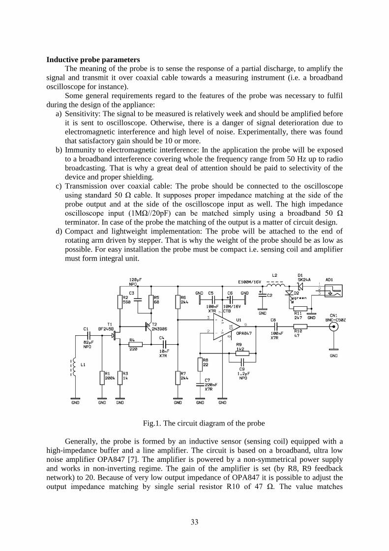
Inductive probe parameters

The meaning of the probe is to sense the response of a partial discharge, to amplify the

signal and transmit it over coaxial cable towards a measuring instrument (i.e. a broadband

oscilloscope for instance).

Some general requirements regard to the features of the probe was necessary to fulfil

during the design of the appliance:

a) Sensitivity: The signal to be measured is relatively week and should be amplified before

it is sent to oscilloscope. Otherwise, there is a danger of signal deterioration due to

electromagnetic interference and high level of noise. Experimentally, there was found

that satisfactory gain should be 10 or more.

b) Immunity to electromagnetic interference: In the application the probe will be exposed

to a broadband interference covering whole the frequency range from 50 Hz up to radio

broadcasting. That is why a great deal of attention should be paid to selectivity of the

device and proper shielding.

c) Transmission over coaxial cable: The probe should be connected to the oscilloscope

using standard 50 Ω cable. It supposes proper impedance matching at the side of the

probe output and at the side of the oscilloscope input as well. The high impedance

oscilloscope input (1MΩ//20pF) can be matched simply using a broadband 50 Ω

terminator. In case of the probe the matching of the output is a matter of circuit design.

d) Compact and lightweight implementation: The probe will be attached to the end of

rotating arm driven by stepper. That is why the weight of the probe should be as low as

possible. For easy installation the probe must be compact i.e. sensing coil and amplifier

must form integral unit.

Fig.1. The circuit diagram of the probe

Generally, the probe is formed by an inductive sensor (sensing coil) equipped with a

high-impedance buffer and a line amplifier. The circuit is based on a broadband, ultra low

noise amplifier OPA847 [7]. The amplifier is powered by a non-symmetrical power supply

and works in non-inverting regime. The gain of the amplifier is set (by R8, R9 feedback

network) to 20. Because of very low output impedance of OPA847 it is possible to adjust the

output impedance matching by single serial resistor R10 of 47 Ω. The value matches

33

approximate value of the cable impedance. Unfortunately, the impedance matching is made at

the expense of additional power loses. The amplifier must drive not only 50 Ω load of

transmission cable but also load of matching resistor. Consequently, the real gain observed at

the end of the cable is only 10. Stage U1 is AC coupled at its input and output as well (see C4,

C7). Low frequency cut-off is set by C7, R8 network.

The DC bias of the U1 stage is set by R6 and R7 resistors. Due to not-negligible input

currents of OPA847 the resistances of R6 and R7 must be relatively low. That applies for R8

and R9 values as well. Unhappily, it results in a low input impedance of the stage that

prevents direct connection to sensing coil. In order to achieve high impedance input of the

circuit the T1 transistor BF245B (N-channel FET) is used there at a first stage. Transistor T2,

2N3906 type, serves as a buffer driving the input of the U1 stage.

The sensing coil is wound on one-half of a toroid ferrite core. The middle diameter of

core is 30 mm. An inductance of the coil together with stray capacitance of the input of the

amplifier (around 5 pF) form resonance circuit. A number of turns necessary for optimal

performance of the probe were adjusted experimentally. The appliance was tested using a

turbo-alternator stator prototype and a calibrating pulse generator. The most powerful

response was received in case of tuning of resonance circuit to approximately 6.1 MHz. The

high-frequency cut-off of the U1 stage was additionally limited to around 30 MHz using C9

capacitor.

The sensing coil and the amplifying circuit form a compact unit. The whole appliance

was implemented on a single printed circuit board (40x65 mm). The unit is shielded by a tin-

plated steel box. The output (BNC) connector, the power input connector and the power LED

can be found at the rear panel of the probe. The probe is powered by external 9V battery.

Fig.2. The probe implementation

Fig.3. Probe response to the

calibration signal

Conclusions

The device for partial discharge measurement and detailed analysis of the stator

winding partial discharge behavior bring to the technical diagnostics of rotating machines

modern and enhanced view to the evaluation of measured data and estimation of lifetime. The

precision localization of partial discharge source within generator winding and the

localization of damaged bars is very important for generator lifetime estimation and for repair

planning.

34

Described method of partial discharge localization and identification using inductive

rotating probe is very powerful tool for service and maintenance of electrical rotating

machines and bring saves and safeness for generator owners.

Acknowledgements

This research was funded by the Ministry of Education, Youth and Sports of the Czech

Republic, MSM 4977751310 – Diagnostics of Interactive Processes in Electrical Engineering.

The authors are grateful for the support of this program.

References

1. Hudon, C.; Torres, W.; Belec, M.; Contreras, R.; , Comparison of discharges measured

from a generator's terminals and from an antenna in front of the slots, Electrical

Insulation Conference and Electrical Manufacturing & Coil Winding Conference, 2001.,

pp.533-536, 2001.

2. Maughan, C.V.; , Turbine-generator condition assessment using Electromagnetic

Interference (EMI) testing, Electrical Insulation (ISEI), Conference Record of the 2010

IEEE International Symposium on., pp.1-5, 6-9 June 2010.

3. H.G. Sedding, S.R. Campbell, G.C. Stone, G.S. Klempner, A New Sensor for Detecting

Partial Discharges in Operating Turbine Generators, IEEE Trans. EC, December 1991.

4. Mentlík. V. Device for rotating probe control, CZ Pattent No. 1981-6619.

5. Mentlík. V Setup for partial discharge diagnostics within dielectric system of rotating

machines,CZ Patent No. 1981-6620.

6. Matsumoto, S.; Three-axis loop antenna for the detection of partial discharge signal,

Electrical Insulating Materials, 2008. (ISEIM 2008). pp.28-31, 7-11 Sept. 2008.

7. Texas Instruments Inc.: OPA847 – Wideband, Ultra-Low Noise, Voltage-Feedback

Operational Amplifier with Shutdown, http://www.ti.com.

Authors Ing. Josef Pihera, Ph.D., Ing. Jiří Švarný, Ph.D.; Department of Technologies and Measurement,

Faculty of Electrical Engineering, University of West Bohemia in Pilsen; Univerzitní 8, 306 14 Pilsen;

e-mail: [email protected], [email protected].

35

Change of dielectric parameters of low voltage cables within the thermal

and ionizing radiation degradations

Procházka R., Ullman J., Hlaváček J. – FEE CTU in Prague

Abstract The paper deals with measurements of degradation processes on low voltage cables which have

important role in supplying of control circuit in nuclear power stations. Two degradation processes

are taking into account the thermal degradation and ionizing radiation. Current practice is based on

application of mechanical tests which shows relatively good results and on their basis is possible to

evaluate the cable condition in the long-term. The main disadvantage is then needs of storing and

taking of samples of all used types of cables in the areas of nuclear reactor. It would be preferable to

use an electrical methods and change of dielectric parameters within the aging when is possible the

individual measurements perform on-site by nondestructive way directly on used cable sets.

Introduction

The low voltage cables have important role under the nuclear power plants conditions.

They primarily serve as cables for supplying of control circuits and they are characterized by

low frequency of operation. So they are not in continuous operation and they should ensure

supplying of control circuits in case of nonstandard operations (accidents) when they cannot

fail. Like any electrical equipment, those cables are exposed to degradation processes which

change electrical parameters of used insulation systems. The main degradation process is

thermal aging. In case of above mentioned control cables may not be a source of heat only the

current flow but also increased temperature of environment in which the cables are stored or

partly increased temperature around various steam-water pipe lines in a nuclear reactor. As

another important degradation factor which can be taking into account under the nuclear

power station conditions is influence of ionizing radiation when the control cables are long-

term exposed to increased level of radiation.

Due to above mentioned facts it is necessary to determined (estimate) the state of

insulation systems of cable sets or try to determine residual life time. Current practice is based

on application of mechanical tests which shows relatively good results and on their basis is

possible to evaluate the cable condition in the long-term. The main disadvantage is then of

course needs of storing and taking of samples of all used types of cables in the areas of

nuclear reactor. It would be preferable to use an electrical methods and change of dielectric

parameters within the aging when is possible the individual measurements perform on-site by

nondestructive way, directly on used cable sets. The influence of degradation processes on

some dielectric parameters of insulation systems was observed within the artificial aging by

using laboratory equipment of company ÚJV Řež, a.s. The results from measurements are

listed below.

Thermal Aging

The main degradation process under consideration is the aging caused by temperature

increasing be the cause current flow or increased temperature of environment in which the

cable is placed. To assess this degradation is most commonly used the Arrhenius model which

expresses the dependence of physical properties on change of temperature

PfeAdt

dP TR

E

, (1)

36

where the P is the observed physical property, A pre-exponential factor, E activation energy,

R gas constant, T absolute temperature and f(P) is a function, which respects the order of

reaction.

Based on this relationship has been established the degradation temperature of each

sample, so that within a defined time frame for measurement (few months) corresponded the

degradation of 50-60 years.

Ionizing Radiation Aging

To assess the influence of ionizing radiation we use the quantities absorbed dose and

dose rate. Absorbed dose D is defined by

dm

EdD , (2)

where the E is the mean energy deposited by ionizing radiation and m is mass.

Absorbed dose represents absorbed energy in unit mass of irradiated substance in

specific point. Dose rate is then given by form

dt

dDD , (3)

where the D is the absorbed dose and t is time.

Dose rate expresses increment of absorbed dose per unit time. The degradation level is

determined on the base of the absorbed dose of each cable samples, when the degradation

time is selected the needed dose power can be determined.

Cable Samples and their Preparation

The degradation processes were performed on the cables type 0,5-CHFE-R 7x1,5

manufactured by Kablo Kladno company (nowadays NKT Cables). In case of thermal

degradation the samples were put on the drums in the oven, where the constant temperature

130°C was maintained. The value of temperature was calculated by using Arrhenius model

(1). The assumption was that at this temperature the cable aging time will match the cable

aging period 50-60 years of its operation in nuclear power plant. With such parameters the

time of degradation will be 50 days. The influence of current loading was simulated by using

of current sources when the part of samples was loaded by constant current. The insulation

system was then degraded by combined thermal heating, from inside and from outside as

well.

When exposed to ionizing radiation, individual samples were wound on drums and

inserted into the irradiation facility, where they were embedded in a cylindrical concrete

wells. In the center of the drum was inserted 60

Co gamma radiation emitter. The dose rate was

regulated by the depth of radiation emitter into the drum. The dose rate was maintained at

0.5 kGy/h. This value is again based on the same assumptions as in the case of thermal

degradation. Samples intended for current loading are again connected to a source of constant

current.

Measurement Description

The process of measurement consisted of two fundamental parts. In the first part

degradation processes took place, in the second part measurement of dielectric parameters.

The transition from first to second part of this process was carried out so that one day before

37

the measurement of dielectric parameters were completed degradation processes of individual

samples. It means, measurements were realized with samples on steady ambient temperature.

Subsequently, the samples were inserted into the degradation environment.

An overview of the measured dielectric quantities is listed below.

Loss Factor and Capacitance

Measurement was realized at the frequency 50 Hz and voltage 1.5 kV. The automatic

measuring Schöring bridge from Tettex Instuments was used.

Capacitance

Measurement of capacitance was realized at frequencies 120 Hz, 1 kHz and 10 kHz.

The Agilent, type U1732B, was used in this case.

Insulation Resistance

The measurement duration was 15, 30 and 60 seconds with applied voltage 500 V. The

CHAVIN ARNOUX, type C.A 6543, resistance measuring instrument was used. The

insulation resistance was measured in two configurations: the middle insulated conductor

against shielding and yellow-green conductor against a blue conductor. All measured values

had similar waveforms. To achieve greater accuracy and measurement quality, the same

connection to the measuring device was kept. Yellow-green wire and shielding was connected

to the ground, resp. to negative electrode in all their configurations. Blue and middle wires

were connected to positive electrode, resp. to phase wire in all their configurations. When

measuring one quantity, the yellow-green wire and shielding were never connected. The same

goes for blue and middle wires.

Mechanical tests of the Tensibility

As a reference measurement in a two-week intervals were taken samples for mechanical

tests of tensibility. Samples for mechanical tests were tested with identical samples used for

electrical measurements. Samples stressed with current load in specified environment were

connected in series. The samples for mechanical tests were modified to make it possible to

measure the tensibility of the conductor insulation.

Mechanical tests were realized with the INSTRON 5543. The stretching speed was

200 mm/minute and the initial distance was 50 mm. The smooth steel jaws 12.5 x 38 mm

(width) were used to fix tested wire. The force which the samples were stretched was 1 kN.

Measured progression during thermal degradation

Measured waveforms of capacity, loss factor, insulation resistance and tensibility during

thermal degradation process are shown in Fig. 1 and Fig. 2.

Fig. 1: Thermal degradation with current load

Fig. 2: Thermal degradation without current

load

38

All measured values were related to the first measured value. Significant changes

occurred very quickly after ten days from the start of degradation processes and these

measured values did not change significantly after the ten-day initial degradation.

Measured progression during ionizing radiation degradation

Measured waveforms of capacity, loss factor, insulation resistance and tensibility during

ionizing radiation degradation process are shown in Fig. 3 and Fig. 4. During this degradation

process dielectric parameters changed significantly in whole the time range of measurement

and in some cases can be traced a trend.

Fig. 3: Ionizing radiation degradation with current

load

Fig. 4: Ionizing radiation degradation without

current load

Conclusions

The measured results show that the thermal degradation of tested low voltage cables

leads to significant changes in dielectric parameters. However for each waveform cannot be

derived the remaining period of life, because after significant initial change, the values are

almost constant in the coming years. In the case of ionizing radiation degradation, dielectric

parameters change significantly during whole the time range of tests and there can be traced a

trend. After the improvement and verification of measurements, could be considered the

usage of measured values changes for determining the residual lifetime of cables.

The most appropriate method for determining the residual lifetime of cables for both

types of degradation processes seems to be a mechanical tensibility tests. Only for monitoring

the effects of ionizing radiation could be considered further experimentation with the

dielectric parameters.

References

1. MENTLÍK, Václav. Dielektrické prvky a systémy. Vyd. 1. Praha : BEN - technická

literatura, 2006. 235 s. ISBN 80-730-189-6.

2. N.H. MALIK, A.A., Al ARAINY, M.I. QURESHI: Electrical Insulation in Power

Systems, Marcel Dekker, New York, 1998.

Authors Ing. Radek Procházka Ph.D., Ing. Jiří Ullman, Ing. Jan Hlaváček; Department of Electroenergetics,

Faculty of Electrical Engineering, Czech Technical University in Prague, Technická 2, Prague 6, 166

27, Czech Republic; e-mail: [email protected], [email protected].

39

Comparison of infrared spectroscopy techniques for transformer oils

analysis

Prosr P., Polanský R. – FEE UWB in Pilsen

Abstract Fourier transform infrared spectroscopy (FT-IR) is a suitable method for measuring of spectra of

liquid samples, which intensely absorb the infrared radiation. Based on absorbed frequency spectrum,

it is possible to detect aging processes. Two different measuring techniques of Infrared spectroscopy

(Attenuated Total Reflectance technique ATR and measuring in transmission mode) are compared and

their sensitivity on thermal ageing at 120 °C of regenerated mineral oil is presented in the paper.

Introduction

Infrared spectroscopy is a measuring technique using different material ability to absorb

the frequency of IR ray. Based on absorbed frequency spectrum, it is possible to determine

different chemical compounds, molecular structure in the sample and their changes as

consequence of ageing process.

Problems related to identification of different material components are considered to be

very important objective. For this purpose, Infrared Spectroscopy has been successfully used,

mainly in chemical industry, food processing industry, or in medicine.[1-4] This paper is

focused on application of Infrared Spectroscopy into electrical technology branch, to a

measurement and interpretation of insulating liquids spectra. In this manner, it is possible to

identify the beginning ageing process caused by thermal oxidation or nitration of the oil.

Infrared spectroscopy of insulating liquids

To the most widely known techniques of the infrared spectroscopy of liquid samples

belongs Attenuated Total Reflectance technique (ATR) and measuring in transmission mode.

Mentioned techniques were compared using sample of regenerated mineral oil. Spectra were

measured along an accelerated thermal ageing at 120 °C. During the ageing, the oil was

placed into glass vessels and stayed closed by reason of the partial restriction of air access. A

sampling was realized at times after 0, 200, 240, 300, 500, 650 and 750 hours of thermal

ageing.

Measuring of FT-IR spectra using Attenuated Total Reflectance technique (ATR)

Figure 1 shows a measuring principle of ATR technique, and ATR measurement setup.

ATR

Crystal

Infrared

Beam

To Detector

Sample in contact

with evanescent

wave

Evanescent

wave

~ mm

Fig. 1. Measuring principle of ATR technique and ATR measurement setup

Detection

crystal

40

The sample is placed on a detection crystal when being measured. A part of the IR ray

aiming at the sample causes absorption in the sample when passing through the crystal-

sample interface (evanescent wave) and thus weakens this part in the final spectrum.

The measurement proceeded with ZnSe crystal, when 32 scans with a resolution of 4

cm-1

were collected for each sample. Spectra were measured with count of 3 and subsequently

averaged using software OMNIC. An automatic correction of spectra baseline had been done

before the evaluation. The subsequent analysis of measured spectra was performed by

OMNIC software too. Figures 3 present the spectra from the ATR measurements.

REGENERAT_DS-ATRREGENERAT_0200h-120°C-ATRREGENERAT_0240h-120°C-ATRREGENERAT_0300h-120°C-ATRREGENERAT_0500h-120°C-ATRREGENERAT_0650h-120°C-ATRREGENERAT_0750h-120°C-ATR

-0,00

0,02

0,04

0,06

0,08

0,10

0,12

0,14

0,16

Abs

orba

nce

1000 2000 3000

Wavenumbers (cm-1) Fig. 2. ATR Spectrum of the aged regenerate oil

Measuring of FT- IR spectra in transmission mode

Measuring technique in transmission mode focuses on detection of IR ray passing

through the sample placed in a liquid cuvette (see Fig. 3). Optical path of the IR ray is chosen

according to the measured liquid in the range from 0,2 to 0,5 mm. KBr or NaCl are thought as

the most suitable materials for the cuvette, however they have inconvenient hygroscopic

properties. Hence it is necessary to prevent them from water or water vapour.

Measuring in transmission mode was proceeded with a resolution of 1 cm-1

in BaF2 cell

with thickness of 1 mm. The subsequent analysis of measured spectra was performed by

OMNIC software too. Figures 4 present the obtained spectra from the transmission mode of

measurement.

Infrared Beam

Fig. 3. Construction of an FT-IR transmission cell (demountable FT-IR liquid cell)

REGENERAT_DS-ATRREGENERAT_0200h-120°C-ATRREGENERAT_0240h-120°C-ATRREGENERAT_0300h-120°C-ATRREGENERAT_0500h-120°C-ATRREGENERAT_0650h-120°C-ATRREGENERAT_0750h-120°C-ATR

-0,005

0,000

0,005

0,010

Ab

sorb

ance

1700 1800 1900

Wavenumbers (cm-1)

Energy absorbed due

to C-H bonds

stretching Energy absorbed due

to C-H bonds

bending Refining

degree Products of ageing –

carbonyl band

41

REGENERAT DS 120°C (average)REGENERAT 0200h 120°C (average)REGENERAT 0240h 120°C (average)REGENERAT 0300h 120°CREGENERAT 0500h 120°C (average)REGENERAT 0650h 120°C (average)REGENERAT 0750h 120°C (average)

1

2

3

4

5

6A

bso

rban

ce

1000 2000 3000 4000

Wavenumbers (cm-1)

REGENERAT DS 120°C (average)REGENERAT 0200h 120°C (average)REGENERAT 0240h 120°C (average)REGENERAT 0300h 120°CREGENERAT 0500h 120°C (average)REGENERAT 0650h 120°C (average)REGENERAT 0750h 120°C (average)

0,3

0,4

0,5

0,6

0,7

0,8

0,9

Ab

sorb

ance

3600 3700

Wavenumbers (cm-1)

REGENERAT DS 120°C (average)REGENERAT 0200h 120°C (average)REGENERAT 0240h 120°C (average)REGENERAT 0300h 120°CREGENERAT 0500h 120°C (average)REGENERAT 0650h 120°C (average)REGENERAT 0750h 120°C (average)

1

2

3

4

5

6

Ab

sorb

ance

1600 1700 1800

Wavenumbers (cm-1) Fig. 4. Spectrum from the transmission mode of measurement

Results and discussion

Focused on the insulating oil ageing, thermal oxidation and nitration are the most

important processes that can be detected by FT-IR technique.[5] Thermal oxidation, as a

reaction of oxygen and oil molecules resulting in degradation of the insulating oil properties,

is largely accelerated by increasing temperature. Spectral bands of oxidation are placed

around frequency of 1746 cm-1

. This carbonyl band is significant evidence of

transesterification of the free fatty acids. [6]

On the other hand nitration is a process when organic compounds turn into nitrogen

oxides (NO, NO2 and N2O4) at increased temperature. These oxides are then in contact with

the oil, which results in organic nitrates. Analogous to oxidation, nitration effects the oil

quality, e.g. by viscosity increase or creation of insoluble substances and sediments [5].

As we can see from figures 3 and 4, sensitivity of the measuring in transmission mode is

much higher compared to ATR. Regarding to a spectral area of oxidation (1746 cm-1

)

technique ATR identify impact of aging markedly later in comparison of transmission mode

of measurement. Change of carbonyl group using ATR technique is detected from 300 hours

of ageing (at 120 °C), while using transmission mode of measurement is detectable for times

200 and 240 hours of ageing.

Antioxidant

Nitration

Oxidation

Decreasing

intensity

within

ageing

Decreasing

intensity

within

ageing Increasing

intensity

within

ageing

42

Nitration products have an intensive absorbance from 1650 to 1600 cm-1

(a band of

nitrate -O-NO2 bonds). ATR technique is less sensitive compared to transmission mode – see

Fig. 2 and 4.

Conclusion

Thermal oxidation and nitration influence the insulating oil properties negatively. The

identification of these processes in mineral insulating oil is considered as very important

objective in power engineering. Oxidation products, mainly acids, support the increase of oil

acidity and thus contribute to the corrosive activity of the oil. Nitrates creating together with

the oxidation products affect the oil properties also very negatively.

Results of the experiment demonstrate the differences between measured techniques of

infrared spectroscopy. As obvious from obtained spectra, the technique of measuring in

transmission mode is expressively more sensitive compared to ATR method.

Acknowledgements

This article was carried out by the help of Ministry of Education, Youth and Sports of

Czech Republic, MSM 4977751310 – Diagnostics of Interactive Processes in Electrical

Engineering.

References

1. Downey G. Food and food ingredient authentication by mid-infrared spectroscopy and

chemometrics, rends in analytical chemismy. TrAC Trends in Analytical Chemistry, Vol.

No. 17, (August 1998), 418-424, ISSN 0165-9936.

2. Yan-ling Zhang; Jian-bo Chen; Yu Lei; Qun Zhou; Su-qin Sun; Isao Noda Discrimination

of different red wine by Fourier-transform infrared and two-dimensional infrared

correlation spectroscopy. Journal of Molecular Structure, Volume No. 974, (June 2010),

144-150, ISSN 0022-2860.

3. Jackson M.; Mantsch H. H. The medical challenge to infrared spectroscopy. Journal

of Molecular Structure, Vol., No. 408/409, (June 1997) 105-111, ISSN 0022-2860.

4. Jackson M.; Sowa M. G.; Mantsch H. H. Infrared spectroscopy: a new frontier in

medicine. Biophysical Chemistry, Volume 68, (October 1997), 109-125,

ISSN 0301-4622.

5. Robinson N.; Hons B. Sc. Monitoring oil degradation with infrared spectroscopy,

Available from: http://www.wearcheck.com/literature/techdoc/WZA018.pdf Accessed:2011-01-17.

6. Liao R., Hao J.., Yang L.,Liang S., Yin J Improvement on the Anti-aging Properties of

Power Transformers by Using Mixed Insulating Oil High Voltage Engineering and

Application (ICHVE), 2010 International Conference, October 2010.

7. Heise, H.M.; Kupper L.; Butvina, L. N. Attenuated total reflection mid-infrared

spectroscopy for clinical chemistry applications using silver halide fibers. Sensors and

Actuators B Vol., No. 51, (August 1998) 84-91, ISSN 0925-4005.

Authors Ing. Pavel Prosr, Ph.D., doc. Ing. Radek Polanský, Ph.D.; Department of Technologies and

Measurement, Faculty of Electrical Engineering, University of West Bohemia in Pilsen; Univerzitní 8,

306 14 Pilsen; e-mail: [email protected], [email protected].

43

Diagnostic methods in the quality control system in the production of plastic materials for direct food contact Samsonek J. – ITC Zlín, Vaculík L. – TESCOMA Zlín Abstract The assessment of the health safety of products for food is regulated by European legislation on plastic materials and articles intended to come into contact with food. In plastic products, one of the risk factors is heavy metals in the plastic matrix. The well-known analytical method for establishing metal content in the plastic product is the technology of microwave decomposition of the plastic and its evaluation using the ICP-OES or AAS analytical methods. Both methods provide results with an accuracy of µg/kg, although in terms of time it takes several hours. However, for on-line control of the manufacturing technology the critical parameters of the products need to be diagnosed within minutes. Hence the requirement to introduce a faster diagnostic methods in the real time of the manufacturing process. One of the possible solutions for screening the metal content in plastic matrices is the application of X-ray fluorescence (XRF). Introduction

The assessment of the health safety of products for food is regulated by European legislature in Commission Regulation (EU) No.10/2011 on plastic materials and articles intended to come into contact with food, which is the Implementing Regulation of the European Parliament and the Council No. 1935/2004 on materials and articles intended to come into contact with food and the repeal of guidelines 80/590/EEC and 89/109/EEC. In Czech legislation these safety requirements are regulated by decree of the Czech Ministry of Health No. 38/2001 Col., which incorporates the above quoted European law and in addition stipulates requirements for materials that are presently not regulated by European directives.

An important part of the consumer market for products intended to come into contact with food consists of plastics. In these products, one of the risk factors is heavy metals, that may originate especially from unapproved pigments or additives. Currently, eight hazardous metals (Pb, Cd, Hg, Cr, As, Se, Sb, Ba) are monitored. The final plastic product may be contaminated by these elements in the form of salts in the applied pigments, functional fillers, etc.

Requirements for plastic materials intended to come into contact with food in terms of the content of toxic heavy metals are as follows:

1) Requirements for the metal content in the pigment extract of up to 0.1M HCl, expressed in per cent of pure pigment, see Appendix No. 1 of Decree No.38/2001 Col. or Resolution of the Commission No. AP 89 (1).

Metal Pigment mass

limit (mass %) antimony 0.05 arsenic 0.01 barium 0.01 cadmium 0.01 chrome - except Cr(VI) 0.1 lead 0.01 mercury 0.005 selenium 0.01

44

2) With regard to the legal requirement for colouring and printing on products intended

to come into contact with food it is not allowed to use colouring agents based on the compounds of antimony, arsenic, hexavalent chrome, cadmium, lead, mercury and selenium.

The standard analytical method for establishing the metal content in a plastic product is

the technology of microwave decomposition of the material in a mixture of acids (HNO3, HCl, HF, H2SO4), peroxides, etc. Commercially used plastics usually decompose at temperatures of up to 205 oC at a pressure of 2.5 MPa and within 30 minutes. The resulting mineralisate is subsequently evaluated in terms of the metal content using the ICP-OES or AAS analytical methods. Both methods provide results with an accuracy of µg/kg, but it takes several hours. With regard to on-line control of the manufacturing technology the critical parameters of the product need to be diagnosed within minutes. Hence the requirement to introduce a faster diagnostic method (if possible non-destructive) in the real time of the manufacturing process.

One of the possible solutions for screening the metal content in plastic matrices is the application of X-ray fluorescence (XRF).

X-ray fluorescent spectrometry (XRF) is an analytical instrumental method taking advantage of the spectral composition of X-ray fluorescent radiation to identify and establish the quality of elements in solid and liquid samples. Most often simpler XRF spectrometers are employed in large production units, and they have become something of a standard in cement plants, oil refineries and geological laboratories. In cement plants they are even used as process analysers with feedback to the ratio of the raw materials feed. Little or no processing of the sample for the analysis and the speed of the concurrent measurement of dozens of elements predetermine XRF as a fast diagnostic method. The principle of the measurement is the interaction between the sample and X-ray radiation. Once X-ray radiation strikes the atom the photon energy is sufficient for knock an electron (so-called photoelectron) out of one of the orbits close to the nucleus (K, L, M). The atom makes a transition into an excited ionised state which is unstable.

The return of the atom to the original state by the migration of an electron from higher levels to the free position is accompanied by the secondary emission of a photon – so-called fluorescence. The energy of the secondary photon (~ wavelength) is clearly linked to atom type. By analysing the spectrum of the fluorescent radiation we can therefore determine the composition of the sample in terms of the type and number of the represented atoms. Fig.1 shows the typical XRF spectrum of a plastic matrix contaminated by lead.

To ensure that the diagnostic method using XRF is comparable with the precision ICP

and AAS analytical methods, our experience shows that the XRF apparatus for analysing plastics needs to be calibrated for at least three types of matrix:

- hydrocarbon - chlorinated (simulating PVC) – up to 50% chloride in the matrix - silicone (simulating polydimethylsiloxane - silicone)

45

Fig.1: XRF spectrum of a plastic matrix contaminated by lead

By unifying the matrix of the sample of the calibration standard, measurement error is reduced. The calibration range is at the 0-100 mg/kg level for Pb, Cd, Hg, Cr, As, Se, Sb, Ba, while this analysis is still considered to be screening and positive results are confirmed by wet methods (AAS, ICP). The reasons for this are the powerful matrix effects of, for example, fillers that can essentially change responses of the individual analyses in real samples. Nevertheless, for the confirmation of negative samples with regard to the presence of toxic heavy metals in plastic matrices this diagnostic model is quite sufficient, fast and efficient. In addition to the confirmation of positive results of ICP or AAS it was possible to carry out an analysis of certified reference material ERM-EC680k, commercially available from IRMM with certified content of As, Br, Cd, Cl, Cr, Hg, Pb, S and Sb. Although the described method is considered to be screening, the agreement of the results with certified values is very good (Fig.2).

Fig.2: Verification of the correctness of the XRF diagnostic method for heavy metals in a

plastic matrix

46

Conclusion With regard to comparing the certified and the measured values of the content of heavy

metals using the XRF method it was found they were in reliable agreement. This makes the method highly suitable for use in accordance with the good manufacturing practice principles (see Directive of the EC No.2023/2006) for materials and articles intended to come into contact with food. Consistent application of this heavy metal diagnostics in the field of plastic manufacturing brings a higher level of safety of the marketed products. References 1. Helán V.: Automatická spektroskopie, Sborník přednášek, 2-THETA, Český Těšín 2007.

ISBN 978-80-86380-39-1. 2. Samsonek J.: Analýza rizikových prvků v polymerech s využitím XRF, přednáška,

Univerzita Pardubice, červen 2009.

Authors Ing. Jiří Samsonek, Ph.D.: INSTITUT PRO TESTOVÁNÍ A CERTIFIKACI a.s., Třída T. Bati 299, 764 21 Zlín, e-mail: [email protected]. Dr.Ing. Ladislav Vaculík: TESCOMA s.r.o., U Tescomy 241, 760 01 Zlín, e-mail: [email protected].

47

Program for prediction of the rest lifetime of rotary machine insulating

system

Trnka P., Svoboda M., Souček J. – FEE UWB in Pilsen

Abstract The working life of electrical machines is primary affected by the state of insulation system. There is a

lot of diagnostics methods, which helps to understand the momentary state of insulation and to avoid

the possible damage or breakdown of machines. This paper describes a way of prediction of rest

lifetime of electrical rotary machines on the basis of on-line diagnostic methods. Described procedure

is counting rest lifetime on the basis of only one degradation process. This methodology can be

extended to cover all degradation factors. Such expert system provides valuable information and

enables operators to lengthen intervals between off-line measurement, maintenance and/or outages.

Introduction

There is numerous of diagnostic techniques available in these days. In various situations

even economical view is not as important. However, the problems may occur while it comes

to interpretation of the results. It requires great experience and often also good knowledge of

tested machine. Operators use several diagnostic tests, they obtain and store large amount of

measured data. The difficulties they face are to interpret measured values and describe actual

state of a machine. For more effective outage planning a tool is needed which enables to

predict rest lifetime.

Background

When trying to count rest lifetime of a subsystem or device, it is necessary to begin with

choosing of key parameters, which gives relevant information. Generators doesn´t have the

only parameter which can represent the state of a machine. There is a plenty of parameters

which gives us partial information only. Therefore next step is to choose the weakest part of a

machine. It is definitely stator winding bar. The key parameter of stator winding might be

dissipation factor tan δ. There are measuring systems, which measures dissipation factor on-

line, however they are not used in Czech Republic in these days. Other parameters which can

be measured on-line and which gives a lot of information about the state of a machine can be

divided into three groups (with examples):

Electrical parameters – voltage, current, partial discharge activity

Mechanical parameters –shaft, bearing, stator and magnetic circuit vibration

Thermal parameters – winding temperature, cooling medium temperature

Then it is necessary to find dependences of key parameters vs. time of aging. These

dependences are called curves of resistance against affecting load and they are measured in

laboratory usually on laboratory aged samples. By this procedure we can obtain dependences

of sample lifetime on load. These models and lifetime curves works well for high stresses. For

very small stresses some materials do not age, or age very slowly. This phenomenon must be

respected in these models. For counting rest lifetime of electrical machine, it is necessary to

know all degradation factors and to describe degradation processes with highest possible

accuracy.

48

Access to problem solving

Recently, “a beta” version of this procedure is being programmed on Department of

technologies and measurement of University of West Bohemia. This program is respecting

thermal and electrical aging only. It can represent e.g. measuring of stator winding

temperature. This program uses several programming languages. Data are obtained from

digital thermometer by PHP scripts and stored in MySQL database. SQL language was

chosen because of its high modularity. Complete expert system must be modular, because

each rotary machine uses various diagnostic devices with various diagnostic signals.

This program is based on web programming languages. They offer great mobility and

the user interface can be displayed anywhere as a dynamic web page. There are no problems

with combination of different web languages in whole application. A big advantage of this

setup is a possibility of control of a numerous objects from one center. On the other hand for

this application the weakest part might be relatively low computing performance. It can be a

problem while using wide data stream, which are typical for example for vibrations measuring

or quadratic calculation over the database. This question must be discussed when designing

the complex expert system.

SQL database

Object parameters Object monitoring

User

Measuring

device

Calculation

loop

Web server

requirements

answers

Off-line

diagnostics

input

PHP scripts

Fig. 1: Program structure

Machine producer expect exact lifetime while designing the machine. This can be taken

as the beginning of the program. Next script is checking new records in database. If there is a

new record, the script rates the actual aging on the basis of actual load. The time between two

measuring is multiplied with resulting aging factor and subducted from rest lifetime. This

procedure is shown on Fig.2.

49

t

Measured

values

Aging

models

Time

kMOD tRELx

Comparison

Database

Fig. 2: Program calculation loop

As new data are obtained from measuring devices, consumed lifetime is counted. Of

course, there is a lot of important details which must be treated, e.g. averaging, sensor drop

out, signal loss or distortion. This procedure enables to observe values of measured

parameters, but also to observe first derivative of the progress, which means kurtosis of

change. This is very important for prediction of imminent failure.

Program uses flash scripts for dynamic charts drawing, so operation can see the state of

machine represented by observed parameters and actual load together almost in real time.

Next to reduce demands on operation a methodology for evaluating the state of rotary

machines is integrated to program [5]. This methodology uses five letters A – E for describing

actual state of machine. A stands for long-term working without a necessity of maintenance

and E means that machine has to be put out of operation immediately. So operation should

only monitor, whether the state is not changing. It gives only a brief overview about the state.

For deeper view there are the charts, mentioned above.

Next important aspect is off-line diagnostics input. The accuracy of actual state

diagnosis is limited by accuracy of models and number of monitored parameters. The aim of

this system is not to predict exact time of failure, but to observe the state of the diagnosed

device and to detect possible deterioration failures. Within outage it is necessary to revise and

check, whether the state estimated on basis of on-line diagnostics correspond also off-line

diagnostics results. Off-line diagnostics always has its importance, because all potential faults

cannot be found out by on-line diagnostics.

The accuracy of prediction is proportional to period between outages.

Experiments

For a proper description of the aging or degradation of a subsystem or component of an

electrical device it is necessary to have information about the degradation process. As an

example of such as results life time curves of the slot insulation are presented in Fig. 3.

The aging of the slot insulation material NEN was performed using both 50 Hz ac

voltage and high frequency square waveform voltage with parameters: rise time 65 ns, 6 kHz,

pulse width 10 μs. Various magnitudes were used to obtain life time curve of the tested

material. Time to breakdown of each sample was recorded in order to get life time data. Life

time curves have been established (Fig. 3).

50

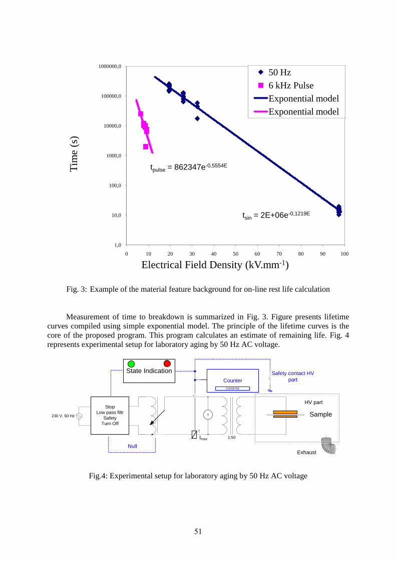
Fig. 3: Example of the material feature background for on-line rest life calculation

Measurement of time to breakdown is summarized in Fig. 3. Figure presents lifetime

curves compiled using simple exponential model. The principle of the lifetime curves is the

core of the proposed program. This program calculates an estimate of remaining life. Fig. 4

represents experimental setup for laboratory aging by 50 Hz AC voltage.

1:50

V

Imax

Safety contact HV

partCounter

Sample230 V, 50 Hz

Stop

Low pass filtr

Safety

Turn Off

State Indication

Null

HV part

Exhaust

123456789

Fig.4: Experimental setup for laboratory aging by 50 Hz AC voltage

tsin = 2E+06e-0,1219E

tpulse = 862347e-0,5554E

1,0

10,0

100,0

1000,0

10000,0

100000,0

1000000,0

0 10 20 30 40 50 60 70 80 90 100

Tim

e (s

)

Electrical Field Density (kV.mm-1)

50 Hz

6 kHz Pulse

Exponential model

Exponential model

51

Conclusions

This access to the problem solving can give relatively good data about the rest lifetime

of observed device. It is however quest for the future to understand all the degradation

processes and have physically based life time curve for each degradation factor or have

multifactor aging description for such as stress. General, it is always more or less accurate

estimation. Expert system cannot fully replace experienced diagnostician. However it can be a

tool which can coordinate all diagnostic signals of an electrical machine, observe actual state

and compare it with history of the machine parameters and loads, estimate rest lifetime. This

could be very useful for machine operators. It can make the interval between outages longer

and reduce maintenance costs effectively.

Acknowledgement This study was carried out with the support of the NADACE ČEZ of the Czech

Electrical Energy Manufacturer and by project of the Ministry of Education, Youth and Sports

of Czech Republic, MSM 4977751310 – Diagnostic of Interactive Processes in Electrical

Engineering.

References

1. Mentlík, V., Pihera, J., Polanský, R., Prosr, P., Trnka, P.: Diagnostika elektrických

zařízení. ISBN 879-80-7300-232-9. Praha: BEN 2008, In Czech

2. Schmidt G., Thien D., Ewert F., Biesemann M., Gradinarov P.: Online and offline

diagnostics as a succesfull interaction for CBM on turbogenerators, International

Conference on Condition Monitoring and Diagnosis, September 6-11, Tokyo, Japan,

2010.

3. Mentlík V., Trnka P.: Aspekty zjišťování spolehlivosti elektrických zařízení –

generátorů, Elektro odborný časopis pro elektrotechniku, č.1 – leden 2011, pp 6-10,

ISSN 1210-0889, FCC Public, In Czech

4. Mentlík V. , Trnka P. – Zvyšování životnosti component energetických zařízení v

elektrárnách, Srní 2010, ISBN 978-80-7043-931-9, In Czech

5. Mentlík V., Trnka P.: Metodika pro hodnocení stavu elektrických zařízení – soubor

metodik pro projekt MPO FI-IN5/173, 2010, In Czech

Authors doc. Ing. Pavel Trnka, Ph.D., Bc. Michal Svoboda, Ing. Jakub Souček,; Department of technologies

and measurement, Faculty of Electrical Engineering, University of West Bohemia in Pilsen,

Univerzitní 8, 306 14 Plzeň; e-mail: [email protected]. [email protected],

[email protected].

52

Detecting Non-Homogenity of Electrically Conductive Adhesives Tučan M., Žák P., Urbánek J. – FEE CTU in Prague Abstract With a rapid expansion of temperature-sensitive technologies, such as Organic LED light sources and displays, it is clear that a reliable and stable technology is required to mount them safely on circuit boards. From the obvious reason of thermal stress, classic soldering is unusable, as peak temperatures for these technologies are often below 100°C. This situation is usually solved by the use of Electrically Conductive Adhesives (ECA), consisting of resin (usually epoxy) matrix and conductive filler (usually silver). However, while this technology solves the temperature problem, it still poses numerous significant risks for reliability. One of such risks is non-homogenity of the adhesives. This was observed on numerous occassions and, in some combinations of ECA and curing temperature, it appeared massively, endangering even the basic dunctions of given circuits. This paper shows the observed cases of serious non-homogenity of ECAs, as well as possible methods to detect it and to set up manufacturing process properly. Introduction

Joints made with electrically conductive adhesives (ECA) contain, in contrast to solder joints, organic compounds that exhibit specific characteristics in the practical application in the technological process of creating joints. During the process of curing, bubbles are formed in the adhesive and they do not escape from the body of the joint due to adhesive’s viscosity. The existence of these bubbles in the joint significantly reduces the internal homogenity, and thus their reliability and stability. The aim of this study was to find procedures to minimize these adverse effects.

Such inhomogenities can have mutliple effects. About the only positive effect would be augmenting the mechanical strength of ECA joints. However, negative effects prevail. Inhomogenity reduces effective electrical contact surface, leading to an increase of current density and thus to higher heating of the joint. Bubbles can readily absorb water vapor, the absorbed water then acts to further degrade the joint during temperature and climatic cycles. Spreading of the adhesive below the component during curing also threatens to dangerously diminish the isolation distance between contact or to outright create short-circuit. Electrically conductive adhesive

Electrically conductive adhesives consist of two parts – adhesive and filler. Basic material – adhesive – is usually epoxy or acrylic resin. Electrically conductive filler is most often based on silver flakes. If we chose epoxy resin, there are two major groups of adhesive – one and two-component adhesives.

Application conditions are more favorable when one-component ECA are used. When using one-component adhesives, process quality depends only on technology of dispenser filling by the adhesive, because we have to prevent the introduction of air bubbles into the dispenser. Another possibility is to remove all air bubbles from the filled dispenser with vacuum. Adverse fact is that the one-component ECA generally have higher viscosity than the two-component adhesives (650 000 - 750 000 cps for one-component ECA [1] and 250 000 – 290 000 cps for mixed two-component ECA [2]).

Technologically, the situation is more complicated in case of two-component adhesives, where it is necessary to mix both components. In some cases, the technological problem is to avoid incorporation of air bubbles during the mixing process, particularly in relation to the

53

actual viscosity. The viscosity of ECA changes significantly during aging, even before the ECA´s expiration date. For this reason, the main focus of our experiment was aimed at application technology of two-component adhesive. Experiments

Experimental part was divided into three parts. In order to minimize the cost of testing the following experiments aimed at the issue of mixing were made using standard epoxy adhesive instead of ECA. For experiments with dispenser filling, a two-component adhesive was chosen and for experiments with the mixing proces, standard two-component phenolic adhesive was chosen.

In the first phase, samples of epoxy resins from different manufacturers were used, in the second phase, some samples of the resin with a metal filler were used. All the experiments were designed to minimize an occurrence of air bubbles in the joints during the application of these adhesives.

In most samples of two-component adhesives without fillers the viscosity significantly decreased temporarily after both components were mixed together. This decrease in viscosity was significant only for a limited period of time, but during this period, the spontaneous release of air bubbles occurred and the vast majority of air bubbles brought by mixing the processed was released. Mixed adhesive was practically free of air bubbles before the use.

In the second part of the experiment, two samples of adhesive filled with steel dust were tested. Temporary decrease in viscosity during the mixing process of two-component adhesive with filler was proved too, but smaller than in the case of the filler-free epoxy.

The same is true for standard two-component ECA (phenolic ECA with 55 ± 1% of Ag filler) [2]. In addition, expired ECA has higher viscosity. This is generally applicable to all epoxy resins and thus the problem with the removal of air bubbles increases.

We can say that the epoxy adhesive, not only the ECA, is usually technically processable, even after the expiration period, but with no guarantees of originally declared parameters. Long-term stability

According to previous studies, adverse results of experimental accelerated aging of ECA joints are mainly caused by the gradual formation of mechanical defects in the structure of cured resin material. Underpressure is creating in cavities of cured adhesive after the curing and subsequent cooling that result in formation of mechanical stress in the structure of joints. This tension is probably the primary cause of cracks in the joints that allow the corrosion in microcracks in the joints. This hypothesis is supported by decrease in ohmic resistance of joint in early stage of aging in dry heat test and the consequent increase in the damp heat test. This phenomenon adversely affects the reliability and current-carring capacity of joints. [3]

Invasive detection of non-homogenity

Tests performed to this day to evaluate the non-homogenity of cured ECAs were generally the same as tests during which the phenomenon was first observed. Two branches of destructive testing were used: optical analysis of cross-sections and mechanical measurement of shear strength of the ECA joints. Results are shown in following figures.

While the non-homogenity is clearly visible in the cross-sections and the shear-off strength showed clearly how the non-homogenous „foam“ formed by AX 20 ECA increased shear strength, these tests were expensive and time-consuming. This limits their usefulness for the industry.

54

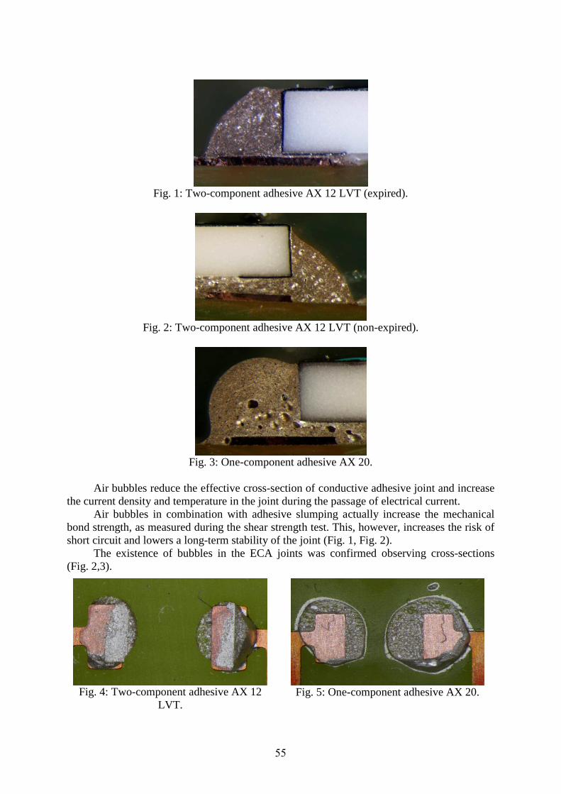
Fig. 1: Two-component adhesive AX 12 LVT (expired).

Fig. 2: Two-component adhesive AX 12 LVT (non-expired).

Fig. 3: One-component adhesive AX 20.

Air bubbles reduce the effective cross-section of conductive adhesive joint and increase

the current density and temperature in the joint during the passage of electrical current. Air bubbles in combination with adhesive slumping actually increase the mechanical

bond strength, as measured during the shear strength test. This, however, increases the risk of short circuit and lowers a long-term stability of the joint (Fig. 1, Fig. 2).

The existence of bubbles in the ECA joints was confirmed observing cross-sections (Fig. 2,3).

Fig. 4: Two-component adhesive AX 12

LVT.

Fig. 5: One-component adhesive AX 20.

55

This phenomenon will be the subject of further investigation and testing – especially the utilization of vacuum during the technological process.

Non-invasive detection method

During a research on ECAs conducted on the department of Electrotechnology, it was found that the non-homogenity may be detected successfully using non-invasive measurement. The experiment used high-level current pulses (100 A), with voltage on the specimen being measured using an oscilloscope.

While in homogenous sample the pulse was clean, with non-homogenous sample partial discharges in the bubbles caused the pulse to be deformed and affected by noise. This allowed for quick sorting of homogenous and non-homogenous specimens.

While this method is yet crude and requires refining to be reliable and repeatable, it would allow for a simpler and less time-consuming preliminary separation of homogenous and non-homogenous samples, not only in laboratory, but probably in real operation as well.

Conclusions

As shown, the ECAs are not the best substitute for SnPb solders for its little resistance to mechanical and climatic stress. Special care has to be given to the non-homogenities, as they tend to augment any problems caused by climatic influence and also change mechanical properties of material and may lead to short-circuits or may severely reduce maximal sustainable power density. Partial discharges may also deform any signal transmitted through the joint.

However, ECAs are the only technically and economically applicable connecting materials for temperature-sensitive electronic components used in the electrotechnical industry. Low-temperature solders may be an environmentally acceptable alternative in such cases, but their price is usually higher than that of ECAs and often their mechanical properties may be found lacking. Acknowledgement

This work was supported by the Grant Agency of the Czech Technical University in Prague, grant No. SGS10/163/OHK3/2T/13. References 1. AMEPOX Microelektronics Ltd.ECO-SOLDER™ AX 20 (one-components ECA). 2. AMEPOX Microelektronics Ltd. Elpox AX 12LVT (two-component ECA). 3. Žák, P., Tučan, M., Kudláček, I. Combined Accelerated Climatic Tests of Electrically

Conductive Adhesives. Electroscope EDS č. 3 2010. ISSN 1802-4564.

Authors Ing. Pavel Žák, Ing. Marek Tučan, doc. Ing. Jan Urbánek, CSc.; Department of Electrotechnology, Faculty of Electrical Engineering, Czech Technical University in Prague; Technicka 2, 16627 Prague 6; e-mail: [email protected], [email protected], [email protected].

56

Measurement of railway traction transformer using by SFRA method – part 1 Brandt, M., Michalík, J. – FEE UŽ Žilina, Kuchta, J . – EVPÚ Nová Dubnica Abstract The paper deals with measurement of railway traction transformer using by Sweep Frequency Response Analysis method (SFRA). This method was tested first time in this scope. In this paper are given reference measurements as well as measurements after type test of new railway transformer. Introduction

Single-phase railway traction transformer consists of a primary winding designed to voltage from 0 to 25 kV and of secondary winding for traction motors power supply. There are also windings for auxiliary locomotive drives power supply and for electrical heating power supply (eventually for air condition) placed on a common magnetic circuit. Traction transformer is exposed during operation of the railroad to frequent mechanical shocks and vibrations. It may cause mechanical breakdowns of transformer windings and core, such as winding displacement (axial or radial), the release of the core and turn-to-turn faults. Detection of these types of failures of traction transformer is possible only by its removal, except the turn-to-turn faults (measurement of winding resistance). Using the SFRA method (Sweep frequency response analyse) to detect those types of traction transformer disorders becomes hot topic, whereas the SFRA method detect the same types of faults on power transformers used in distribution or transmission systems [1]. For frequency characteristics measuring by SFRA method we have chosen a prototype of the traction transformer, developed by EVPÚ Inc., Nová Dubnica in cooperation with ŽOS Vrútky Inc. The measurement of traction transformer by SFRA method has been realised in the Slovak Republic for the first time. There are published only the basic parameters of traction transformer in the article. There is also published the measurement methodology, we designed and implemented as well as the basic reference waveforms of SFRA characteristics. Traction transformer parameters and measurement methodology Table 1: Basic traction transformer label data

Fig. 1: Winding wiring diagram of traction transformer prototype

Power kVA 4900 Primary. voltage

V 25 000

Secondary. voltage

V 2x1700 / 2x1500

Primary. current

A 196

Secondary. current

A 2x1226 / 2x233

frequency Hz 50

57

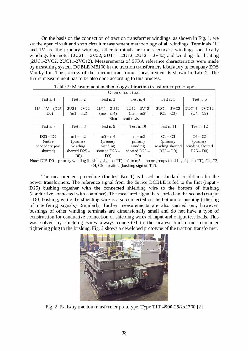
On the basis on the connection of traction transformer windings, as shown in Fig. 1, we set the open circuit and short circuit measurement methodology of all windings. Terminals 1U and 1V are the primary winding, other terminals are the secondary windings specifically windings for motor (2U21 – 2V22, 2U11 – 2U12, 2U12 – 2V12) and windings for heating (2UC1-2VC2, 2UC11-2VC12). Measurements of SFRA reference characteristics were made by measuring system DOBLE M5100 in the traction transformers laboratory at company ZOS Vrutky Inc. The process of the traction transformer measurement is shown in Tab. 2. The future measurement has to be also done according to this process.

Table 2: Measurement methodology of traction transformer prototype Open circuit tests

Test n. 1 Test n. 2 Test n. 3 Test n. 4 Test n. 5 Test n. 6

1U – 1V (D25 – D0)

2U21 – 2V22 (m1 – m2)

2U11 – 2U12 (m5 – m4)

2U12 – 2V12 (m4 – m3)

2UC1 – 2VC2 (C1 – C3)

2UC11 – 2VC12 (C4 – C5)

Short circuit tests

Test n. 7 Test n. 8 Test n. 9 Test n. 10 Test n. 11 Test n. 12

D25 – D0 (entire

secondary part shorted)

m1 – m2 (primary winding

shorted D25 – D0)

m5 – m4 (primary winding

shorted D25 – D0)

m4 – m3 (primary winding

shorted D25 – D0)

C1 – C3 (primary

winding shorted D25 – D0)

C4 – C5 (primary

winding shorted D25 – D0)

Note: D25-D0 – primary winding (bushing sign on TT), m1 to m5 – motor groups (bushing sign on TT), C1, C3, C4, C5 – heating (bushing sign on TT).

The measurement procedure (for test No. 1) is based on standard conditions for the

power transformers. The reference signal from the device DOBLE is fed to the first (input - D25) bushing together with the connected shielding wire to the bottom of bushing (conductive connected with container). The measured signal is recorded on the second (output - D0) bushing, while the shielding wire is also connected on the bottom of bushing (filtering of interfering signals). Similarly, further measurements are also carried out, however, bushings of other winding terminals are dimensionally small and do not have a type of construction for conductive connection of shielding wires of input and output test loads. This was solved by shielding wires always connected to the nearest transformer container tightening plug to the bushing. Fig. 2 shows a developed prototype of the traction transformer.

Fig. 2: Railway traction transformer prototype. Type T1T-4900-25/2x1700 [2]

58

Measured reference characteristics The following figures show the reference waveforms of traction transformer, which was

first measured by the method SFRA. These waveforms are part of the prototype tests, which were performed on the transformer.

Fig. 3: Measured reference frequency characteristics of traction transformer by SFRA method for open circuit measuring methodology

Fig. 4: Measured reference frequency characteristics of traction transformer by SFRA method for short circuit measuring methodology

59

Conclusions

Using SFRA method for measuring traction transformer is the next application of preventive diagnostic. Because of, we cannot determine individual types of failures, next research in this area is needed. The continuity and analysis of the SFRA measured characteristics of traction transformer after type tests is given in the paper entitled Measurement and analysis of railway traction transformer using by SFRA method 2., which is also placed in this proceeding.

Acknowledgement

This paper was done within the project APVV-0703-10 – Analysis and diagnostic measurements of power transformers using by Sweep Frequency Response Analysis. References 1. M. Gutten, Brandt, M. ; Polanský, R. ; Prosr, P: High-frequency analysis of three-

winding autotransformers 400/121/34 kV In: Advances in electrical and electronic engineering. - ISSN 1336-1376. - Vol. 7, [spec.] No. 1-2 (2008), p. 134-136.

2. http://www.siea.sk/inovativny-cin-roka-2010/c-1056/vysledky-sutaze-o-cenu-ministra-hospodarstva-sr-inovativny-cin-roka-2010/.

Authors Ing. Martin Brandt, PhD., prof. Ing. Ján Michalík, PhD.; Department of Measurement and Application, Faculty of Electrical Engineering, University of Žilina, Veľký Diel , 01026 Žilina; e-mail: [email protected], [email protected]. doc. Ing. Jozef Kuchta, PhD., EVPU Inc., Nová Dubnica, Trenčianska 19, 018 51 Nová Dubnica, [email protected] .

60

Measurement and analysis of railway traction transformer using by SFRA method – part 2 Brandt, M., Seewald, R., Sedlák, J., Faktorová, D. – FEE UŽ Žilina Abstract The paper is built on the article entitled Measurement of railway traction transformer using by Sweep Frequency Response Analysis Method (SFRA). The analysis of measured frequency response is described. The transformer was subjected to the type tests and to subsequent exchange of bushing on the primary winding. Introduction

As it was already mentioned in previous paper, the aim is at measurements on a prototype of the railway traction transformer, type T1T-4900-25/2x1700. The transformer was subjected to all type tests, required for setting them into operation. The tests were made in the laboratory of traction transformers at ŽOS Vrútky Inc. and in laboratory of Electrical Engineering Faculty and Computer Science at Slovak Technical University in Bratislava (SFEI STU Bratislava). After basic measurements like measurement of windings resistance, measurement of insulation, open circuit measurement, short circuit measurement, and so on, the transformer was measured by SFRA method and reference SFRA waveforms were recorded. The bushing on the primary winding D25 was damaged during surge voltage test. It was removed and superseded by a new one, which was subsequently also tested. Transformer was again transferred from laboratory in Bratislava into the laboratory in Vrútky and was again subjected to SFRA tests. Measurement and analysis of SFRA characteristics of railway traction transformer after type tests

The repeated measurement of SFRA characteristics of traction transformer were realized according to Table 1. Because of the transformer part damage (bushing on primary winding D25) caused during the previous tests, mainly because of surge voltage test, it was necessary to made a measurement of SFRA characteristics again, and find out how it affects waveforms shape as well as to analyse if there could occur mechanical changes on the transformer windings.

Table 1: Methodology of railway traction transformer measurement Open circuit tests

Test n. 1 Test n. 2 Test n. 3 Test n. 4 Test n. 5 Test n. 6

D25 – D0 m1 – m2 m5 – m4 m4 – m3 C1 – C3 C4 – C5

Short circuit tests

Test n. 7 Test n. 8 Test n. 9 Test n. 10 Test n. 11 Test n. 12

D25 – D0 (entire

secondary part shorted)

m1 – m2 (primary winding

shorted D25 – D0)

m5 – m4 (primary winding

shorted D25 – D0)

m4 – m3 (primary winding

shorted D25 – D0)

C1 – C3 (primary

winding shorted D25 – D0)

C4 – C5 (primary

winding shorted D25 – D0)

Note: D25-D0 – primary winding (bushing sign on TT), m1 to m5 – motor groups (bushing sign on TT), C1, C3, C4, C5 – heating (bushing sign on TT).

61

Waveforms in Fig. 1 and 2 show the impact of the primary winding bushing D25 exchange on the shape of traction transformer SFRA characteristic. Due to the large number of measured characteristics, we introduce only the reference waveforms and also the waveforms from the primary winding tests D25 – D0 (Test No. 1 and 7).

Fig. 1: SFRA characteristics of traction transformer – open circuit measurement (D25-D0)

Reference waveform waveform from type tests

Fig. 2: SFRA characteristics of traction transformer – short circuit measurement (D25-D0)

Reference waveform waveform from type tests

62

Fig. 3: Analysis of waveforms D25-D0 (reference and from type tests) for open circuit

measurement methodology using cross-correlation coefficient

Fig. 4: Analysis of waveforms D25-D0 (reference and from type tests) for short circuit measurement

methodology using cross-correlation coefficient In Fig. 3 and 4, the waveforms of the primary winding characteristics analysis are

shown. The primary winding analysis was realized by cross-correlation coefficients for the reference measurements and for measurements after type tests. The Cross-correlation coefficients (CCFs) are used directly in Doble company´s software and are needed for the exact interpretation of the measured waveforms according to Table 1 with regard to defined values of these coefficients according to Table 2 [1].

CCFs are often used in industry, telecommunications, and where the exact signal analysis is important. Application of Cross-correlation in the SFRA is of importance at two waveforms analysis. If the computed values of coefficients are 1.0, it is an absolute correlation and if values are 0.0, it is an absolute noncorrelation. The negative correlation coefficients are of no importance at assessment by SFRA method [1].

63

Table 2: Explanation of CCFs examples

CCF

good agreement 0.95 – 1.0

boundary agreement 0.90 – 0.94

bad agreement < 0.89

discord <= 0.0

CCFs are defined by equation:

( )( )

( ) ( )22

1

∑∑

∑

−⋅−

−−= =

YYXX

YYXXCCF

ii

n

iii

, (1)

where Xi and Yi are two real series (or graphs in the case of SFRA) compared to every individual frequency “i”, X and Y are the axis of values. In the case of mathematical signal processing, which is more complex, the coefficient values are between 1 and -1 still accurate for the necessary conclusions. [1] Conclusions

On the basis of the analysis of Fig. 3 and 4 and based on automatic cross-correlation coefficient calculation, we can specify that the replacement of damaged bushing D25 had an impact on the reference waveforms shape. However, a major waveform shape change do not occurred and waveforms are within the allowable limits, as set out in Table 2. These measurements confirmed that whatever mechanical change is represented by change in SFRA characteristic shape. In our case, it was an exchange of one bushing, which was recorded as a slight change in the waveform D25-D0 shape. Other measurements also show that during tests there was no other winding or core damage. And we propose to consider the new measurement after tests as a new reference one, which will serve for comparing with other waveforms, measured throughout the whole period of the operation of this traction transformer prototype. Acknowledgement

This paper was done within the project APVV-0703-10 – Analysis and diagnostic measurements of power transformers using by Sweep Frequency Response Analysis. References 1. Kennedy, G., M., McGrail, A., J., Lapworth, J., A.: Using Cross-Correlation Coefficients

to Analyze Transformer Sweep Frequency Response Analysis (SFRA) Traces., 1-4244-1478-4/07, IEEE PES Power Africa 2007.

Authors Ing. Martin Brandt, PhD., doc. Ing. Dagmar Faktorová, Ing. Jozef Sedlák , PhD., Ing. Róbert Seewald; Faculty of Electrical Engineering, University of Žilina, Univerzitná 1, 010 26, e-mai: [email protected], [email protected] [email protected], [email protected],

64

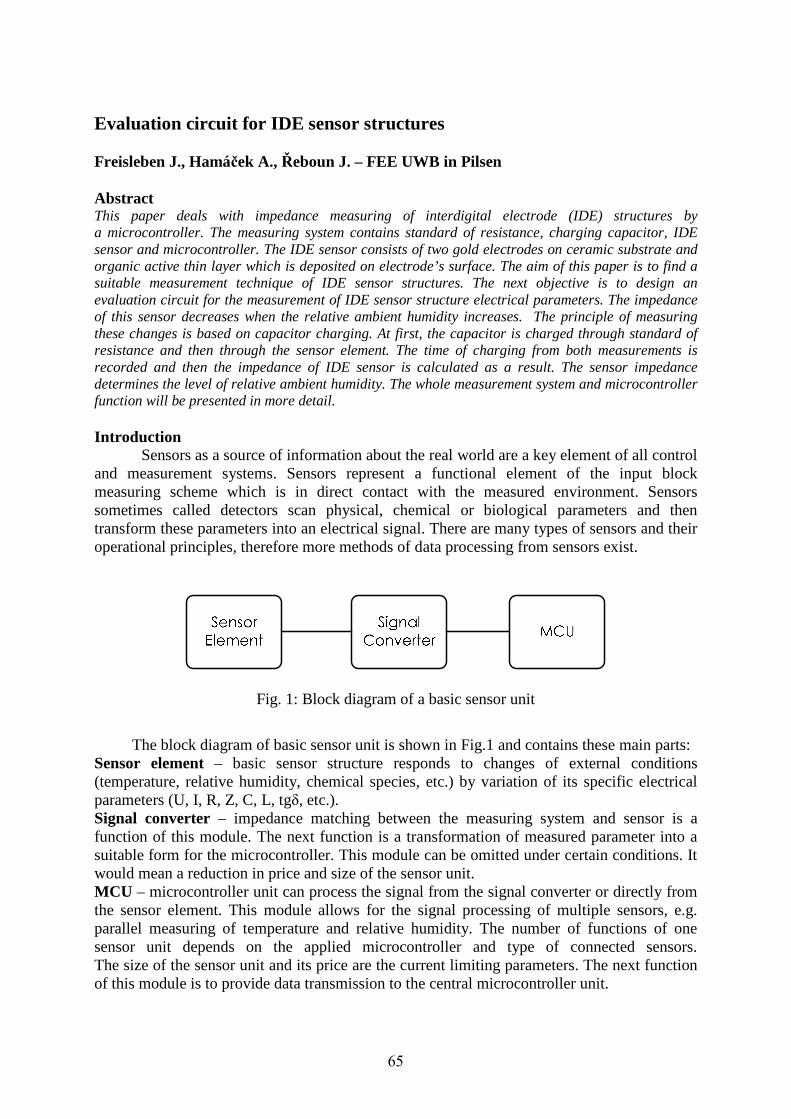
Evaluation circuit for IDE sensor structures Freisleben J., Hamáček A., Řeboun J. – FEE UWB in Pilsen Abstract This paper deals with impedance measuring of interdigital electrode (IDE) structures by a microcontroller. The measuring system contains standard of resistance, charging capacitor, IDE sensor and microcontroller. The IDE sensor consists of two gold electrodes on ceramic substrate and organic active thin layer which is deposited on electrode’s surface. The aim of this paper is to find a suitable measurement technique of IDE sensor structures. The next objective is to design an evaluation circuit for the measurement of IDE sensor structure electrical parameters. The impedance of this sensor decreases when the relative ambient humidity increases. The principle of measuring these changes is based on capacitor charging. At first, the capacitor is charged through standard of resistance and then through the sensor element. The time of charging from both measurements is recorded and then the impedance of IDE sensor is calculated as a result. The sensor impedance determines the level of relative ambient humidity. The whole measurement system and microcontroller function will be presented in more detail. Introduction Sensors as a source of information about the real world are a key element of all control and measurement systems. Sensors represent a functional element of the input block measuring scheme which is in direct contact with the measured environment. Sensors sometimes called detectors scan physical, chemical or biological parameters and then transform these parameters into an electrical signal. There are many types of sensors and their operational principles, therefore more methods of data processing from sensors exist.

Fig. 1: Block diagram of a basic sensor unit

The block diagram of basic sensor unit is shown in Fig.1 and contains these main parts: Sensor element – basic sensor structure responds to changes of external conditions (temperature, relative humidity, chemical species, etc.) by variation of its specific electrical parameters (U, I, R, Z, C, L, tgδ, etc.). Signal converter – impedance matching between the measuring system and sensor is a function of this module. The next function is a transformation of measured parameter into a suitable form for the microcontroller. This module can be omitted under certain conditions. It would mean a reduction in price and size of the sensor unit. MCU – microcontroller unit can process the signal from the signal converter or directly from the sensor element. This module allows for the signal processing of multiple sensors, e.g. parallel measuring of temperature and relative humidity. The number of functions of one sensor unit depends on the applied microcontroller and type of connected sensors. The size of the sensor unit and its price are the current limiting parameters. The next function of this module is to provide data transmission to the central microcontroller unit.

65

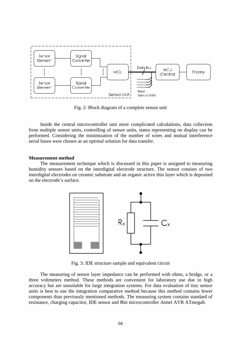
Fig. 2: Block diagram of a complete sensor unit

Inside the central microcontroller unit more complicated calculations, data collection from multiple sensor units, controlling of sensor units, status representing on display can be performed. Considering the minimization of the number of wires and mutual interference serial buses were chosen as an optimal solution for data transfer.

Measurement method

The measurement technique which is discussed in this paper is assigned to measuring humidity sensors based on the interdigital electrode structure. The sensor consists of two interdigital electrodes on ceramic substrate and an organic active thin layer which is deposited on the electrode’s surface.

Fig. 3: IDE structure sample and equivalent circuit

The measuring of sensor layer impedance can be performed with ohms, a bridge, or a three voltmeters method. These methods are convenient for laboratory use due to high accuracy but are unsuitable for large integration systems. For data evaluation of tiny sensor units is best to use the integration comparative method because this method contains fewer components than previously mentioned methods. The measuring system contains standard of resistance, charging capacitor, IDE sensor and 8bit microcontroller Atmel AVR ATmega8.

66

1

2

T

TRR NormalSensor ⋅=

Fig. 4: Evaluation circuit of integration comparative method and integration time relation graph

The resistive part of sensor impedance dominates in this measuring, so the sensor

capacity is neglected. The principle of integration comparative method is based on capacitor charging.

At first, the capacitor CNormal is charged through the standard of resistance RNormal and then through the sensor element resistance RSensor. The time of charging from both measurements is recorded by a microcontroller and then the resistance of the sensor is calculated as a result. Microcontroller unit manages the capacitor charging through output ports and detects voltage changes on input of the embedded analog comparator (Fig. 4). The embedded reference voltage is connected on the comparator positive input. The 16bit timer was used for precise time measuring. The timer starts counting at the beginning of charging. When the voltage of negative input is bigger than positive input the analog comparator stops the counting of the timer. This situation is the same for charging through RNormal and RSensor

and the whole charging process is fully controlled by a microcontroller. We can calculate the resistance of sensor RSensor from recorded time values T2, T1 and from standard of resistance RNormal (see Fig. 4). This sensor resistance determines the level of relative ambient humidity.

Conclusion The alternate measuring is important for IDE sensors structure because these sensors

show partially ion conductivity. Direct measuring causes an ion migration of sensor material from one electrode to another. The organic material can start to transport itself from one side to the other side and this causes a gradual increase in impedance. This situation is obviously undesirable.

The integration comparative method is suitable for IDE sensor structure because it is based on alternate charging and discharging of the capacitor. The advantage of this method is that it is not necessary to use an extra precise capacitor from the point of view of temperature

67

stability, supply voltage fluctuations and long term stability. These parameters are compensated by the comparative measuring method. The resultant accuracy depends on standard of resistance RNormal and on microcontroller parameters. For this measuring the Atmel AVR ATmega8 microcontroller was chosen because of very low input leakage current of analog comparator (IACLK) which is only 50 nA.

The functionality of this method was tested on the development board with the microcontroller. The maximum measured value of resistance is in the range of hundreds MΩ. We can expect better result for the final design of PCB, where short connections will reduce the inductance and the interference will be minimized.

Acknowledgment This paper was supported by the project MPO-TIP FR-TI1/144 MULTISENSORG:

“Multi-component electronic systems based on organic compound”. References 1. Ďaďo, S., Kreidl, M.: Senzory a měřící obvody, ISBN 80-01-02057-6 Praha : ČVUT

1996. 2. Matoušek, D.: Práce s mikrokontroléry ATMEL AVR ATmega16. ISBN 80-7300-174-8

Praha : BEN 2006. 3. Atmel AVR ATmega8 - Katalogový list. San Jose (California) : Atmel Corporation

2008. Authors Ing. Jaroslav Freisleben, doc. Ing Aleš Hamáček, Ph.D., Ing. Jan Řeboun, Ph.D.; Department of Technologies and Measurement, Faculty of Electrical Engineering, University of West Bohemia in Pilsen; Univerzitní 8, 306 14 Pilsen; e-mail: [email protected], [email protected], [email protected].

68

Use of Internet as an instrument for control of measurement instruments in materials diagnostic Frk M., Rozsívalová Z. – FEEC BUT Brno Abstract The article discusses the use and interconnection of information technology and practical applications of measurement in the diagnostic. It focuses primarily on the description of the laboratory network allowing connection of any measurement instruments, which are equipped with data communication interfaces. An integral part of the text is a description and a software support to ensure access and control of measurement instruments over Internet. Introduction

With the development of modern technologies and the availability of high-speed Internet is increasingly encountered with moving desktop applications to the Internet. Individual applications are then accessible via a web browser, which is part of any operating system. In the same way it is possible to make accessible not only theoretical information and simulations in the form of a virtual laboratory, but also controlling of measuring instruments and access to practical measuring applications using the laboratory computer network. Interconnection of information technology and practical applications of measurement then represents a complete e-learning tool that is wider use in education [3]. On-line access to the measuring devices in materials diagnostic

The idea of creating a remote access to measuring devices over the Internet represents the interconnection areas of information technology and practical applications of diagnostic methods. In the particular case it is a remote control of devices intended for diagnostics and monitoring of the structure properties of dielectric and semiconductor materials in the following areas - "The influence of humidity and frequency components of the complex permittivity Electrical Ceramics", "Effects of thermal stress on the courses of absorption characteristics of insulating materials", "Determination of C-V characteristics of MOS structures", "Determination of temperature dependence of the components of complex permittivity of ferroelectric materials based on ceramics titanic" and "Analysis of the properties of ferroelectric materials in an electric field".

Remote Desktop Connection

The scheme of initial connection and arrangement of measuring devices used for selected diagnostic methods is shown in Figure 1. The personal computer is available within each diagnostic method which is primarily intended for software control a locally connected measuring instrument. Each computer is then plugged into the faculty computer network with Internet access and has a fixed IP address. The simplest way to provide remote access to such measuring devices is to connect users to local computer using Remote Desktop, which is part of the most common Windows XP and later versions. It is then possible to use measuring devices with software identical manner as if the user was connected directly in the laboratory. The solution allows to control measuring device over the Internet but in any case is about remote access to the measuring equipment because is used for access the Remote Desktop via another computer. Besides the need for personal computers is a major disadvantage the presence of measurement internal GPIB (General purpose Interface Bus) card or external USB / GPIB interface and GPIB connecting cables.

69

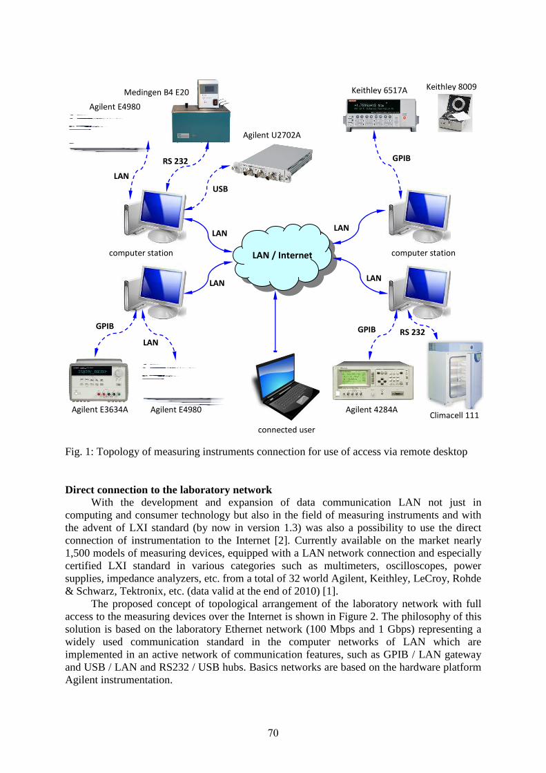
Fig. 1: Topology of measuring instruments connection for use of access via remote desktop

Direct connection to the laboratory network With the development and expansion of data communication LAN not just in

computing and consumer technology but also in the field of measuring instruments and with the advent of LXI standard (by now in version 1.3) was also a possibility to use the direct connection of instrumentation to the Internet [2]. Currently available on the market nearly 1,500 models of measuring devices, equipped with a LAN network connection and especially certified LXI standard in various categories such as multimeters, oscilloscopes, power supplies, impedance analyzers, etc. from a total of 32 world Agilent, Keithley, LeCroy, Rohde & Schwarz, Tektronix, etc. (data valid at the end of 2010) [1].

The proposed concept of topological arrangement of the laboratory network with full access to the measuring devices over the Internet is shown in Figure 2. The philosophy of this solution is based on the laboratory Ethernet network (100 Mbps and 1 Gbps) representing a widely used communication standard in the computer networks of LAN which are implemented in an active network of communication features, such as GPIB / LAN gateway and USB / LAN and RS232 / USB hubs. Basics networks are based on the hardware platform Agilent instrumentation.

computer station

Agilent E4980

LAN / Internet

connected user

computer station

Medingen B4 E20

Agilent U2702A

Agilent E3634A

Keithley 6517A

USB

RS 232

LAN

Keithley 8009

GPIB

Agilent 4284A Climacell 111

GPIB

LAN

GPIB RS 232

Agilent E4980

LAN LAN

LAN LAN

70

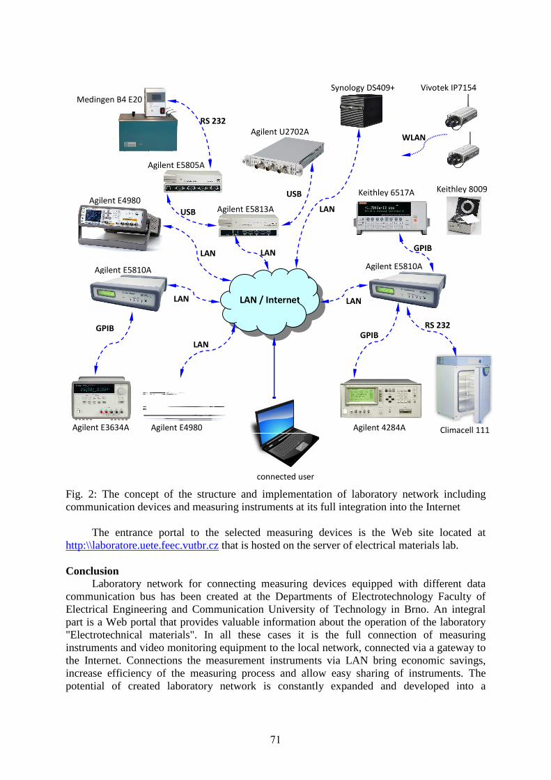
Fig. 2: The concept of the structure and implementation of laboratory network including communication devices and measuring instruments at its full integration into the Internet

The entrance portal to the selected measuring devices is the Web site located at

http:\\laboratore.uete.feec.vutbr.cz that is hosted on the server of electrical materials lab.

Conclusion Laboratory network for connecting measuring devices equipped with different data

communication bus has been created at the Departments of Electrotechnology Faculty of Electrical Engineering and Communication University of Technology in Brno. An integral part is a Web portal that provides valuable information about the operation of the laboratory "Electrotechnical materials". In all these cases it is the full connection of measuring instruments and video monitoring equipment to the local network, connected via a gateway to the Internet. Connections the measurement instruments via LAN bring economic savings, increase efficiency of the measuring process and allow easy sharing of instruments. The potential of created laboratory network is constantly expanded and developed into a

Agilent E5810A

Agilent E4980

Medingen B4 E20

Agilent U2702A

Agilent E3634A

Keithley 6517A Keithley 8009

Agilent 4284A Climacell 111 Agilent E4980

Agilent E5805A

Agilent E5810A

Agilent E5813A

LAN / Internet

USB

RS 232

LAN GPIB

LAN

GPIB

GPIB

LAN

connected user

LAN

Synology DS409+

USB

RS 232

WLAN

Vivotek IP7154

LAN LAN

71

comprehensive system through which it will be possible to control the complete management of laboratory instruments.

Acknowledgments

Authors would like to thank the Ministry of Education, Youth and Sport for financial contribution provided by a grant FRVŠ 344/2011/F1/a - "Modernizace materiálově orientovaných úloh prostřednictvím internetového přístupu" and BUT by a grant FEKT-S-11-7 - "Materiály a technologie pro elektrotechniku". Laboratory equipment has been achieved with financial support FRVŠ under this project. References 1. The LXI Consortium. LXI Products [online]. 2010 [cit. 2011-03-20]. Dostupný z WWW:

http://www.lxistandard.org/products/. 2. Manaloto, M. The Next Generation of Test, LXI and Agilent Open [online]. 2010 [cit.

2011-01-15]. Dostupný z WWW: http://www.tti-test.com/go/lxi/lxi-pdfs/An_Introduction_to_LXI.pdf.

3. Frk, M., Rozsivalová, Z. Internet access to measuring equipments in diagnostics. In DISEE 2010. Bratislava: STU v Bratislavě, 2010. ISBN: 978-80-227-3366- 3.

Authors Ing. Martin Frk, Ph.D., Ing. Zdenka Rozsívalová; Department of Electrotechnology, Faculty of Electrical Engineering and Communication, Brno University of Technology, Technická 10, 616 00 Brno; email: [email protected], [email protected].

72

Dielectric absorption of insulating system generators in operation

Hájková L., Petr J., Hájek J. – FEE CTU in Prague

Abstract One of the important diagnostic methods used in insulating systems of large rotating electrical

machines is method for measuring charging currents, for which is the dominant part the absorption

currents. Charging currents are measured by diagnostic group ČEZ nearly half a century. These

values were used for measurements of three hydrogenerators and two turbogenerators, for this study.

All used machines have insulation system in temperature class 155 °C. The results were compared

with measurement results for systems with temperature class 130 °C. This article contains graphic

processing of dielectric absorption for the insulation system temperature class 155 °C. This graphic

processing did not show a clear change neither during the thirty years of measuring insulating

systems of these machines.

Introduction

For the evaluation of insulation systems of large rotating machines are used different

diagnostic methods. One of the most important diagnostic methods is measuring of charging

current and this method is also used by diagnostic group ČEZ. The theoretical basis of this

method was created in older types of insulation systems created by split mica, paper and

asphalt or shellac. For the newer types of insulation systems made from epoxy composite

(epoxy resin), glass fabric and regenerated mica, this diagnostic method has been loaned and

on the basis of laboratory measurements [2] confirmed by theoretical assumptions obtained by

examining the older types of insulation systems. Purpose of this study was to show the

behavior of absorption curves for new types of insulation systems using the values obtained

by measurements on factual large rotating machines. For purposes of this work were used

values of three hydrogenerators and two turbogenerators producing power for Czech

Republic. Measured values were taken from the protocols of measuring diagnostic group

ČEZ.

Evaluation theory of absorption currents:

Charging currents are the sum of absorption currents and conduction current, and they

can be evaluated by various methods. It proceeds especially, the use of various indices and

constants or graphical representations. Because conductivity current in the real measurements

and dry insulation forms a negligible part, we can evaluate the charging currents as absorption

currents. This study converse of evaluating graphically plotted absorption curves, depending

on the time from the beginning of movement of the machine and time slope of the values k

and n constants that describes the machines isolation state.

The course of absorption current in the insulation system is the sum of exponentials

wide range of migration polarizations and it can be simply described by a power function:

, (1)

where i, is the absorption current, t is time and k and n are already mentioned constants.

To simplify evaluation the state of this isolation is a power function used in logarithmic

form:

. (2)

73

Time dependence of the absorption current is then displayed as a line, whereas the

constants k and n are describing the shift and course of lines. Constant k describes shift in

vertical direction and constant n relative angle to the x-axis.

Beyond absorption curves are there plotted time-dependences of constants k and n (at

the time of operation). These constants represent the absorption curves. Constant k describes

the magnitude of the absorption current and constant n describes the rate of decline of the

absorption current at the time of measurement.

In the evaluation of absorption currents are used graphical representations. It is

generally known (from practical measurements), that in the older types of insulation systems

are absorption curves staged in logarithmic coordinates as lines. With the aging of insulation

systems lines are moving up and slightly tilts against the x-axis. This tendency was confirmed

in laboratory conditions, even on samples of a new type of insulation system [2].

Graphical evaluation of the absorption currents curves:

There were plotted absorption curves in the first part of this study for all phases of three

machines examined DC charging voltage. On the picture Fig.1 is an example of dependence

of selected absorption curves for one of the surveyed machines (Dalešice TG3) for one phase

with a DC charging voltage of 5, 10 and 15 kV. The results were similar at the other

machines.

Fig. 1: Absorption current phase U hydrogenerator Dalešice TG3 for DC charging voltages 5

kV, 10 kV and 15 kV

In the second part of the study were plotted the time dependences of channels on the

time constants of the machine. The picture Fig.2 is an example of corresponding dependences

on the same machine for phase V.

74

Fig. 2: The phase V constants k and n hydrogenerator Dalešice TG3 in DC charging voltage

10 kV (R = 0.96)

For all machines there were calculated correlations between constants k and n at DC

charging voltage of 10 kV. Evaluation of correlation was performed by using the sample

correlation coefficient [4]:

-

-

-

, (3)

where m is the number of measurements, x are values of the constant k and y are values of the

constant n. The statistical significance of the selection correlation coefficient R was then

determined from tables of critical values of the correlation coefficient given in [5].

The values of sample correlation coefficients for the investigated machines are listed

in the table Tab.1. For hydrogenerators was boundary of statistically significant linear

relationship determined by the value of the correlation coefficient 0.7. For turbogenerator

there is the small number of measurements, that´s why not the correlation coefficient R

statistically significant.

Tab. 1: The values of sample correlation coefficients for the investigated machines

Hydrogenerator Phase R

Turbogenerator Phase R

Dalešice TG1

U 0.92

Tisová TG1

U 0.97

V 0.79 V 0.96

W 0.99 W 0.89

Dalešice TG2

U 0.76

Tisová TG3

U 0.68

V 0.82 V 0.85

W 0.87 W 0.86

Dalešice TG3

U 0.78

V 0.96

W 0.94

Conclusions

The main goal of this study was to investigate behavior of absorption currents in newer

types of insulation systems and compare it with the results of measuring on machines with

older types of insulation. In older insulation systems, which were made of split mica, paper,

75

asphalt or shellac, attend to disengaging layers during the life of isolation, and thus the

increase of constants k and n, namely, the absorption curves shift upward and to a slight tilt.

With the newer insulation systems, which are made of epoxy composite (epoxy resin, glass

fabric, mica regenerated), similar phenomenon apparently doesn’t happen. However, the

laboratory measurements were provided in [2] confirmed, that the newer types of insulation

with aging increase the value of the constants k and n again. On the processed values derived

from measurements of real insulation systems of generators this trend didn’t appear. The

question is, why is that so. There are several possible explanations. One of them is the fact

that the investigated insulation systems are not yet in a state where the aging has been

reflected on a state of isolation, and thus on the absorption curves.

The new insulation systems, showed an interesting tendency of absorption curves to

move up and down in the direction of the y-axis and rotate towards the x-axis without rules,

during machine operation. There can be many explanations for this behavior but this study did

not achieve a definite conclusion. So-called “treeing” (creating cracks in the insulation) was

discarded, because for this phenomenon there had to be some humidity, but in the machines,

which are measured out in practice, there isn’t any. Another option is the bursting of

macromolecular chains of epoxy. With creation of low-molecular substances, would happen

increment of absorption in the substance. Both of these phenomena, however, lead to

permanent changes, which can’t clearly confirm the results of measurements.

During comparison the time courses of constants k and n, strong linear relationship

between these waveforms, was noted. The match in rising or falling waveforms constants k

and n is occurred, at inconsiderable percentage of plotted graphs, almost perfectly. The only

difference is in magnitude of rate and value differences between consecutive values. Few

exceptions, selective correlation coefficient R ranges in values higher than 0.7, that indicates a

statistically significant linear relationship between the constants k and n.

The dependence of correlation between the courses of the constants k and n on the size

of charging voltage didn’t appear on the examined machines.

References

1. Radová, L.: Dielektrická absorpce v diagnostice generátorů; Thesis; ČVUT FEL Katedra

elektrotechnologie, Praha 2010; supervised by: Petr, J.

2. Liedermann, K.: Dielektrická relaxační spektroskopie polymerních dielektrik; inaugural

dissertation; VUT FE, Brno 1996.

3. Petr, J., Radová, L., Antfeist, F.: Využití dielektrické absorpce v diagnostice izolace

generátorů; article of Diagnostika’09, Praha 2009.

4. Hátle, J., Likeš, J.: Základy počtu pravděpodobnosti a matematické statistiky; book;

SNTL/ALFA, Praha 1974.

5. Kubanová, J., Linda, B.: Kritické hodnoty a kvantily vybraných rozdělení

pravděpodobností; textbook; Univerzita Pardubice, Pardubice 2006.

6. Protocols of measurement ČEZ.

Authors Ing. Lenka Hájková, Doc. Ing. Jiří Petr, CSc., Bc. Jan Hájek; Department of Electrotechnology,

Faculty of Electrical Engineering, Czech Technical University in Prague; Technicka 2, 16627

Prague 6, e-mail: [email protected], [email protected], [email protected].

76

Noise source identification using sound intensity measurement

Klasna J. – FEEL ZČU UWB in Pilsen

Abstract This papers deals with noise source identification according to ČSN ISO 9614-1 standard. This

method uses the sound intensity measurement in points of the measuring surface. The measuring

surface surrounds the measured device and is divided into the point’s grid. The sound intensity is then

measured in each point of the grid. For better understanding of the measured data it is suitable to

convert the data into the graphical representation. Typical representation of measured data is to

convert them to distribution map. To do this job, the graphical user interface was created in MATLAB.

Introduction

Noise source identification helps to find the main noise sources of the measured device.

The sources can represent individual components of the device and the localization of the

main sources enables reduction of total noise level. Another application of this method is to

find the damaged or defective components of the complex device.

The sound intensity I is vector representation of sound energy flow through a unit area.

It is given by instantaneous sound pressure p and the corresponding particle velocity u (1).

(1)

The value of sound intensity can be measured by sound intensity probe and the orientation of

the probe determinate the direction of the flow of the energy. Typically, the positive value of

sound intensity represents the energy flow from the measured source and the negative value

responds to energy flow to the source. Sound intensity is represented in most cases in level

expression. The measured value is then related with reference value and the dependence is

then logarithmic. The sound intensity level LI is given by (2) and the reference value I0 is

10-12

W.m-2

.

(2)

Sound intensity measurement according to ČSN ISO 9614-1 standard

The measured device must be surrounded by measuring surface. The shape choice of

the measuring surface depends on shape of the measured device. Typical measuring surfaces

are cuboid, hemisphere, cylinder and half-cylinder. The whole device must be inside the

measuring surface and the minimum distance between measuring surface and device must be

kept. After that is the measuring surface divided into the point’s grid (Fig. 1) and the sound

intensity is measured in each point of the grid. The distance between measuring points sets the

space resolution. The distance between points can be various – if it is necessary to have better

resolution in several places of the surface, the grid can be finer in this areas.

The sound intensity is used in this case for determination of sound power. Sound power

P is given by sum of partial sound powers Pi. The partial power is defined as a multiplication

of sound intensity in one point Ii and corresponding partial surface Si (3). Index n represents

number of measuring points on the surface.

;

(3)

77

Fig. 1: Typical measuring surface

Described method has several advantages in comparison with other methods of

determination of sound power. The main advantage allowed to measure the device in real

condition (in real placement – it is not necessary to move the device to the laboratory or to

modify the placement of the device). The measuring distance is relatively small (typically

from 0.5 meter – the measurement can be performed in the near filed). It is also possible to

measure individual parts of complex device.

Fig. 2: Sound intensity map of real device

78

On the other side, there are several limitations of this method. The sound intensity probe

can measure in frequency range from 50 Hz to approximately 10 kHz (but not the whole

bandwidth at the same time – the bandwidth is divided into 3 bands). The noise source must

be stationary (because the whole measurement is relatively lengthy) and other requirements of

the standard must be kept to get reliable results.

Representation of measured results

The desired result of the measurement is hidden in large amount of numbers. For better

understanding of measured data it is suitable to convert the data into the graphical

representation. One of the possibilities is to create the distribution of sound intensity/sound

power on the surface (Fig. 2). The axis represents the size of the measuring surface. The color

bar is located on the right side of map and it shows the value of acoustic intensity. The black

points in the map represent the measuring points of the measured surface. The value of sound

intensity between points is interpolated because of softening of the changes. On this map is

very simple to find the main noise sources.

The software used for creation of the map on Fig. 2 uses MATLAB software for

calculations and displaying results. This software uses graphical user interface (GUI) and

allowed full control over the process of map creation and image export. Exported image with

adjusted transparency can be placed on picture of real device (Fig. 3). Unfortunately, this

program can’t perform this operation yet, so it must be done in other software. GUI offers

clearly arranged control components and is described in more details in [2].

Fig. 3: Sound intensity map placed on image of real device

79

Conclusions

The described method of sound power determination allows localizing the main noise

sources on the measured device. This should be very helpful in case of searching the damaged

or destroyed part of complex device. Indisputable advantage of this method is the possibility

to measure the device in real placement in the company. The main disadvantages are the

frequency limitations (given by sound intensity probe and distance between probe and device)

and large time demand, so the noise must be in time continuous.

The sound intensity map is very useful graphical representation of the measured data,

because it illustrates the distribution of sound intensity on the surface. The developed GUI

simplifies the process of map creation and export.

Acknowledgement

This paper was supported by the research grant FR-TI1/159: Integration of system for

production and modification of compressed air.

References

1. ČSN ISO 9614-1: Akustika – Určení hladin akustického výkonu zdrojů hluku pomocí

akustické intenzity – Část 1: Měření v bodech., Praha: Český normalizační institut, 1995.

2. Klasna J.: MATLAB graphical user interface development for education support. In:

34th International Spring Seminar on Electronics Technology, ISBN 978-80-553-0646-9,

Košice: Technická univerzita v Košiciach.

Authors Ing. Jan Klasna; Department of Technologies and Measurement, Faculty of Electrical Engineering,

University of West Bohemia in Pilsen; Univerzitní 26, 306 14 Pilsen; e-mail: [email protected].

80

Fast controlled transfers process analysis of 6 kV switchgear in NPP Mareček O., Kaška M. – TES s.r.o. Třebíč Abstrakt Fast controlled transfers of the 6 kV switchgears in NPPs are used especially for the reasons of the reactor core cooling ensurance in case of the main power supply failure. This article contains fast controlled transfers behaviour analysis in the event of a close short circuit in the electrical power system. Proper information was obtained thanks to the monitoring and diagnostic system implemented in the NPP. Introduction

The 6 kV switchgear used for main coolant pump motors power supply are equipped with the fast controlled transfers in the Temelín NPP. The main coolant pumps are used for heat transport from the reactor core. A power supply transfer from the main (normal) to stand-by source is occurred in case of a failure of the main power supply system. It is not allowed to activate reactor protections in this case as a result of the power input decrease of the main coolant pumps.

This fast controlled transfers were successfully tested during a commissioning period of both NPP units.

A main transformer failure was occurred in 2004 (the main power supply system). The fast controlled transfer failed and the change to the stand-by power source was made by slow relay automatics. It caused the reactor protection activation due to the power input decrease of the main coolant pumps and finally to the reactor shut down.

The whole event process was recorded by the monitoring system MOSAD®. Causes of the fast controlled transfer failure were discovered thanks to detailed analysis of this monitoring system records. Changes of the fast controlled transfer algorithm were designed and implemented consequently.

Fast controlled transfer automatics of the 6 kV switchgear

The main power supply of the 6 kV switchgears (included switchgears equipped with the fast controlled transfer) is implemented from the 400 kV bulk power substation Kočín through the block and tap-changing transformers. The stand-by (auxiliary) power supply of the 6 kV switchgears is implemented from the 110 kV bulk power substation Kočín through the auxiliary transformers. The 400 kV and 110 kV bus bars are coupled in the Kočín switch yard. Therefore it is possible to change the supply from the main to stand-by power source in synchronism.

The 6 kV switchgears used for main coolant pump are equipped with synchronization relays BECO. This synchronization relay enables to make power supply transfer by its fast channels. If this channels work properly, the power supply transfers come through without reactor protection activation.

The reactor protections are activated in case of low-power relays activation from three of four main coolant pumps. The low-power relay setting is: power P < 0,5 Pn during time t ≥ 0,9 s.

The synchronization relay continuously evaluates voltage amplitude, phase shift and frequency difference between 6 kV switchgear voltage and stand-by power supply voltage. This relay is equipped with three channels, two of them are fast and one slow:

81

− FAST channel. If the synchronization relay activation is occurred (e.g. due to an electrical protection activation) and the phase shift between voltages is ≤ 30°, synchronisation relay sends out a stand-by power source switch closing order. The FAST channel time window is ≤ 200 ms.

− IN PHASE channel. If the synchronization relay activation is occurred (e.g. due to an electrical protection activation) and the frequency difference between voltages is ≤ 4,5 Hz, synchronisation relay sends out a stand-by power source switch closing order in time of zero phase shift. The IN PHASE channel time window is from 0,2 s to 2 s.

− U2 channel. If the synchronization relay activation is occurred (e.g. due to an electrical protection activation) and the switchgear voltage drops on U < 0,3 Un, synchronisation relay sends out a command to switch off all power consumers. The stand-by power source switch closing order is sent out after 70 ms delay.

In addition, there is a slow independent relay automatics in every 6 kV switchgear:

− U1 channel. This relay automatics sends out a stand-by power source switch closing order in case of the switchgear voltage drops on U< 0,4 Un with delay 0,5 s. A low-voltage automatics always switches off all power consumers before the stand-by power source switch is switched on.

Fast controlled transfer automatics of the 6 kV switchgear tests

Several tests evidencing proper function procedure of 6 kV switchgear fast controlled transfers under load were realized in a commissioning period. A test initiation was made by a simulation of electrical protection activation or a 400 kV switch disconnection.

An analog and binary data obtained by MOSAD® monitoring system was successfully used for test analysis. Figure n. 1 shows voltage and current curves of the 6 kV switchgear during FAST channel test. The controlled transfer time was 80 ms. The phase shift between voltages was 13° in the time of stand-by power source switching on.

Fig. 1: Voltage and current curves of the 6 kV switchgear during FAST channel test

82

Figure n. 2 shows voltage and current curves of the 6 kV switchgear during IN PHASE channel test. The controlled transfer time was 720 ms. The frequency difference between voltages was 2,53 Hz in the time of stand-by power source switching on (zero phase shift).

Fig. 2: Voltage and current curves of the 6 kV switchgear during IN PHASE channel test

Block transformer failure The second unit was coupled into power system and worked on the nominal power. A

failure of the third phase block transformer unit was occurred. The generator and the power line 400 kV was switched off . The controlled transfer to the stand-by power source of the 6 kV switchgears was occurred.

The fast controlled transfer failed and the change to the stand-by power source was made by slow relay automatics. It caused to the reactor protection activation due to the power input decrease of the main coolant pumps and finally to the reactor shut down.

The whole event process was recorded by the monitoring system MOSAD®. Causes of the fast controlled transfer failure were discovered thanks to detailed analysis of this monitoring system records:

− A sharp decrease of the 6 kV switchgear voltage in phases L1 and L3 with negative-phase sequence component signalling was occurred. The negative-phase sequence component signalling caused the external blocking of the synchronization relay activation due to the electrical protection activation.

− The main 6 kV power supply switch was switched off due to the electrical protection activation in 70 ms after the start of failure. The main 6 kV power supply switch disconnection blocked the synchronization relay activation.

The controlled transfer was not led through the synchronization relay fast channels but only through the slow external relay U1-channel. Figure No. 3 shows voltage and current curves of the 6 kV switchgear during the controlled transfer by the U1-channel. The whole time of the controlled transfer was 2,47 s.

83

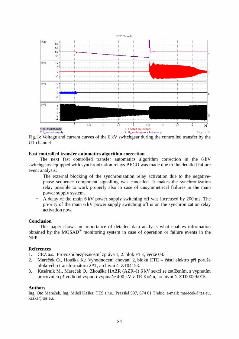
Fig. 3: Voltage and current curves of the 6 kV switchgear during the controlled transfer by the U1-channel Fast controlled transfer automatics algorithm correction

The next fast controlled transfer automatics algorithm correction in the 6 kV switchgears equipped with synchronization relays BECO was made due to the detailed failure event analysis:

− The external blocking of the synchronization relay activation due to the negative-phase sequence component signalling was cancelled. It makes the synchronization relay possible to work properly also in case of unsymmetrical failures in the main power supply system.

− A delay of the main 6 kV power supply switching off was increased by 200 ms. The priority of the main 6 kV power supply switching off is on the synchronization relay activation now.

Conclusion

This paper shows an importance of detailed data analysis what enables information obtained by the MOSAD® monitoring system in case of operation or failure events in the NPP. References 1. ČEZ a.s.: Provozní bezpečnostní zpráva 1, 2. blok ETE, verze 08. 2. Mareček O., Houška K.: Vyhodnocení chování 2. bloku ETE – části elektro při poruše

blokového transformátoru 2AT, archivní č. ZT04153. 3. Kasárník M., Mareček O.: Zkouška HAZR (AZR–I) 6 kV sekcí se zatížením, s vypnutím

pracovních přívodů od vypnutí vypínače 400 kV v TR Kočín, archivní č. ZT00029/015. Authors Ing. Oto Mareček, Ing. Miloš Kaška; TES s.r.o., Pražská 597, 674 01 Třebíč, e-mail: [email protected], [email protected].

84

Energy audit and revisions of power equipments

Šebök M., Gutten M., Kučera M., Korenčiak D. – FEE UŽ Žilina

Abstract Knowledge of problems of measurement in the infrared radiation allows us to use the thermovision diagnostic methods more effectively and to localise the disturbance which determines the quality of electrical wiring and equipments in the inside distribution of electric energy. In carrying out repeated surveys of professional and technical examination of selected technical equipment thermovision is an important diagnostic method for determination in energy audits and revisions of power wiring and equipment. Heated objects with higher temperature near measured objects influences value of measured temperature of these examined electrical equipment.

Introduction Radiation of hot sources acts like (in respect of surrounding conditions), like visible

light. To display temperature fields we can use visualization techniques used in optics. The only differences are materials used for elements of visualization systems, size of values which are derived from the wavelength of radiation, and also sensitivity of sensors for recording the signal. The surface of the measured object in a state of thermodynamic equilibrium emits electromagnetic radiation and the radiated power depends on the thermodynamic temperature and properties of the surface object.

For thermovision diagnostics of infrared radiation in the inside distribution of electric energy, we need to take into account many important factors affecting the accuracy of measurement. Results of the measured values of specific electric contact are often biased by measurement defects. In determining the classification of degrees to correct the defects, it is necessary to correct measured values due to disruptive effects of other objects. [1] Theory Heating is defined by the relationship α/ε, where α is the absorption coefficient of energy and ε is the emission coefficient (emissivity) of the measured body. [2] Ratio of intensity radiation of actual body and ideal black body at the same temperature is defined by spectral coefficient of emissivity:

( )( )TH

THT

,

,),(

0 λλλε

λ

λλ = (1)

It is clear that the coefficient of spectral emissivity is equal to the spectral absorption coefficient. The research on issues of radiation of solid bodies is based on knowledge of absolute black body; an object which is able to fully absorb the full spectrum of radiated energy. By Kirchhoff’s law the black body is an ideal emitter. Plank defines the spectrum of black body radiation:

1

2),( 52

−=

−

kT

hc

e

hc

d

TdH

λ

λπλλ (2)

Spectral radiant flux density of black body surface depends on the length of the wave and temperature. [2]

Plank’s law is a function of spectral distribution of values. Spectral distribution curves dH(λ,T)/dλ entering at temperature T (Fig.1) go through the maxima.

85

Fig.1: Curves of the spectral distribution

Win’s law clearly defines the shift of visible and invisible body radiation (when it is

heated) to the side of the shorter waves. [3] Stefan-Boltzmann’s law, as an integration of Planck's law to λ, defines an integral radiant flux density of black body at the temperature T:

[ ] 4

0

/),( TddTdHH T σλλλ == ∫∞

(3)

σ = 5,67.10-8 W/m2K4 – Boltzmann constant. Derived Planck’s equation on temperature dT, we receive change of spectral flux

density emitted from black body as a function of temperature:

[ ] λλλ

λ

λ

d

dH

eT

ekhc

T

ddHkThc

kThc

.1

)/(/()/(2

)/(

−=

∂∂ (4)

Real objects generally do not behave as black bodies. No-black bodies absorb only a part of α(λ)Φ (incident radiation), part of the reflected radiation ε(λ)Φ and part τ(λ)Φ is transient radiation. If the system is in thermodynamic equilibrium (Fig.2), under the law of conservation of energy reflected and transient energy is equal to the energy absorbed. [3]

Fig.2: Distribution of the incident radiation

Emissivity ε(λ) (coefficient of radiation), compensates absorption coefficient α(λ) then

ε(λ)= α(λ). It follows that: 1)()()( =++ λτλρλε (5)

The result of object temperature measurement T0, which is registered in the spectral range of wavelengths ∆λ (surface density of radiant flux), is the registered radiant flux density Hreg: [ ] [ ] [ ] λλλλελλλλτλλλλρ

λλλ

ddTdHddTdHddTdHH ffaareg ∫∫∫∆∆∆

++= ),()(/),()(/),()( 00 (6)

When an object is transparent τ(λ) = 0 and if T0 is much larger than Ta , the first part of the equation is very small. In this case the task is easier and it is essential to know ε0(λ). Difficulties arise when the body is surrounded by other objects, which have high temperature and these temperatures are higher than the examined object. In this case, its own radiation depends on the T0 and ε0 affected by reflected radiation error caused by parasitic (surrounding) objects with a temperature Te and emissivity εe. (Fig.3). [4]

Incident radiation Φ

ε(λ) emisivity

Transient radiation τ(λ)Φ Reflected

radiation ρ(λ)Φ

α(λ)Φ

Absorbed radiation

86

If the reflection coefficient is measured as ρe - radiation error, then the part characterizing the error is proportional to Te, εe and ρe , Te,

Fig.3 Influence of other radiating objects

For measures of this type it is necessary to know ε0 and T0 parameters and the number of equations, which are equal to number of unknowns. Radiation of measured object is formed by the sum of two parts; own H1 radiation and parasitic H2 radiation in the infrared spectral range: [ ] [ ] λλλλελλλλελρ

λλ

ddTdHddTdHSH eee ∫∫∆∆

+=11

/),()(/),()()( 00 (7)

S - geometric parameter which depends on the distance of two objects and on their surfaces. Experimental

Thermovision measurements warn us about the progressive deterioration of transition resistances of connections, about overheating and deterioration of isolation systems condition, machinery and electrical equipment (Fig.5). [5]

On the Fig.4 we can see the thermogram of measured object BR1 at a temperature T0 and emisivity ε0 which we want to know (radiant breaker BR1 on the left) and from the other side we can see parasitic object with temperature Te, which is larger than T0 (radiant breaker BR2 on the right). Emissivity εe of parasitic object is high and the distance from measured object d is small. The temperature value Te and emissivity εe is unknown. The thermal camera distinguishes this different temperature of objects, i.e. temperature, which would have absolutely black body in this spectral range.

Fig.4: Termogram of breakers in electric Fig.5: Thermogram of electric wiring breaker switchgear

The result of calculated equation is the temperature of parasite object Te = 361, 5ºK. Value of calculated temperature Te=361, 5ºK is near to measured temperature Te = 357.45 ºK. The size of radiation flux density of parasite object BR2 (εe = 0.96 and temperature Te = 357.45 ºK) is: [ ]∫

∆

=1

/),(λ

λλλε ddTdHH eee (8)

Then the radiant flux density of the measured object is:

d

εe, Te

Thermovision system

T0, ε0

(1-ε0) εe, T β

measured object T0,ε0,β0

εe , Te

parasite object Te,εe

BR2 BR1

87

[ ] [ ] λλλεελλλελλ

ddTdHSddTdHH eee ∫∫∆∆

−+= /),()1(/),( 00 (9)

radiation reflection If S=1 then we have result calculated temperature of measured object BR1 T0=303, 15ºK, and for emisivity: 75,0

/)4,357,6,3(1

01

0 ===

−=∫

∆λ

λµλε

dKTmdH

HH e

o

(10)

Following data were calculated: BR1: T0 = 303,15ºK =43ºC, ε0= 0,75 BR2: Te = 361,5ºK = 84ºC, εe= 0,82 Conclusion

Comparing the results of calculated and measured values; we see that real measured temperature values are influenced by parasite object. The differences between the calculated and measured values are illustrated on the graph (Fig.6). On the graph we see measured and calculated temperature differences of breaker BR1 at the current load. Measured temperature of BR1 is higher than calculated because close parasite object influences its temperature. As we can see on the graph (Fig.6) temperature differences depend on the value of current load (In). The results of experimental measurements and mathematical calculations of temperature differences for parasitic object we can see on the graph (Fig.7).

0

20

40

60

80

100

0 10 20 30 40 50 60 70 80 90 1001measured 2calculated

0

20

40

60

80

100

0 10 20 30 40 50 60 70 80 90 1001 measured 2calculated

Fig.6: Dependence of measured and recalculated warming T0 to breaker BR1

Fig.7: Dependence of measured and calculated values of warming Te on breaker BR2

In carrying out repeated surveys of professional and technical examinations of selected technical equipments thermovision is an important diagnostic method for determination in energy audits and revisions of power wiring and equipments. Heated objects with higher temperature near measured objects influences values of measured temperature of these examined electrical equipment. References 1. Šebök, M., Gutten, M., Kučera, S. Kučera, M. Kontrola bezpečnosti a spoľahlivosti

výkonových transformátorov pomocou termovízie. ELDICOM 2009, Žilina, 2009. 2. Benko, I.: Determination of the Infrared surface Emisivity, Budapest, 1990. 3. Toth, D., Infrared System Helps with Energy Efficiency, USA, 1995. 4. Klabacka,E.: Surface modifications for Thermovision Measurement, ČVUT, Praha. 5. Lysenko, V.: Detectors for noncontact temperature measurement, Praha, 2005. Authors Milan Šebök, doc. Ing. Miroslav Gutten, Ph.D, Matej Kučera, Ing. Daniel Korenčiak; Department of Measurement and Application, Faculty of Electrical Engineering, University of Žilina, Veľký Diel , 01026 Žilina; e-mail: [email protected], [email protected], [email protected], [email protected].

T [ºC] [ºC]

In[%] In[%]

T[ºC]

88

Requirements for assessment of LOCA cables VUKI in deliveries for the Mochovce NPP Verbich O., Sulová J., Valach R. – VUKI, a.s., Bratislava Abstract VUKI, a.s., experience in requirements for cable properties for NPP primary zones, their assessment in deliveries and documentation.

The legislative requirements for quality assurance of classified equipment for NPP´s are as follows:

Act No. 541/2004 Coll. on peaceful uses of nuclear energy (Atomic Act). The act deals with the conditions for operation of nuclear installations and the performance of state surveillance over their nuclear safety. Also part thereof is Art. 25 Quality Assurance that addresses the responsibility for determination of and compliance with the requirements for quality of nuclear installations, classified equipment, their categorisation under safety classes in the field of making use of nuclear energy, including supplies of equipment and services. Specific requirements for NPP equipment are subsequently governed by ÚJD SR Decree No. 56/2006 Coll. laying down details of licensee quality system documentation requirements as well as details of quality requirements for nuclear installations and details of the scope of their approval. Specific requirements are addressed by Art. 6 Quality of Nuclear Installations precisely defining the scope of accompanying documentation whereby the supplier is due to demonstrate compliance with the requirements for quality of NPP classified equipment, specific results of testing to prove the nuclear installation resistance to seismicity and environment effects in all test, operational and design emergency conditions. These requirements were encountered in our company while preparing the supplies for NPP Mochovce completion, specifically Units 3 and 4 and VVER 440 reactors.

For VVER 440 reactors the minimum required lifetime for cables is currently 40 years for routine operating temperatures up to 60°C and emergency temperatures up to 127°C. Additionally, they have to comply with demanding and frequently contradictory requirements such as being resistant to ionization radiation, fire-proof and, if possible, halogen-free (exceptions in particular the US and Russia), at the same time with reduced moisture absorption, and they have to satisfy the major leak accident functionality requirements even upon expiry of their use in the primary circuit over a period of 40 years. We were awarded certificates for this type of power and signal cables in 2009 also at VUKI, a.s., with the material and structural design of cables being the result of the company´s own research. The upper side to certificates awarded by VUJE, a.s., which is the only authorized certification body certifying products - classified equipment for Central European nuclear power plants, is that the demonstration of the required 40-year lifetime in given conditions is unambiguous and unquestionable which can be proved with the following results of close to two-year assessment by the certification body of our cables. The conditions for VVER 440 reactors are as follows:

A. Normal operation environment: Maximum operating temperature: 60°C Minimum required functionality: 40 years at a temperature up to 60°C Pressure: atmospheric Maximum relative humidity: 90 % Integrated radiation dose: 280 kGy (installed lifetime 40 years)

89

B. Environment emergency conditions - Loss of Coolant Accident (LOCA) Maximum relative humidity 100 % Radiation conditions - dose rate 1 kGy/hr Integrated gamma radiation dose: (LOCA + post LOCA) 10 kGy Chemical spray: Start: 5 minutes into emergency conditions Duration: 24 hours during prevailing emergency conditions Spray solution temperature: 45 - 60°C Spray solution concentration: 13,7 g/kg H3BO3; 2,7 g/kg KOH; 0,2 g/kg N2H4H2O Overall integrated radiation dose: 319 kGy (for normal and emergency conditions including safety margin +10 %)

Fig. 1: Tensile strength of cable CHKE 4x2,5 LOCA following simulated radiation aging (overall dose in 40 years 319 kGY)

Fig. 2: Ductility of cable CHKE 4x2.5 LOCA following simulated radiation aging (over dose in 40 years 319 kGY)

Fig. 3: Tensile strength of cable JE-H(St)H 2x2x0.8 LOCA following simulated radiation ageing (overall dose in 40 years 319 kGY)

Fig. 4: Ductility of cable JE-H(St)H 2x2x0.8 LOCA following simulated radiation ageing (overall dose in 40 years 319 kGY)

For the above requirements also VUKI, a.s., cables were tested, specifically the

representative of power cables CHKE-V 4x2.5 LOCA and that of signal cables JE-H(St)H-V 2x2x0.8 LOCA, and the following parameters were delivered in assessing their lifetime: The cables thereafter withstood also the test described above, the LOCA simulation, with virtually no change occurring in the cable appearance and with only a minimum change in the assessed functional properties.

Despite these provable results guaranteed by the certification body performing regular surveillance over the production of LOCA cables at VUKI, a.s., it is necessary to further demonstrate for the follow-up supplies their quality and conformity to the requirements for particular reactors, which implies moreover extensive documentation and testing. This is based on developing a Quality Assurance Program containing in addition to the supplier basic data a precise specification of cables to be supplied, including certificates proving their properties. The advantage of the certificates is that the certificate-guaranteed properties need not to be subsequently examined during the delivery of cables e.g. for the Mochovce NPP. In

90

addition to demonstrating the fitness for VVER 440 (VUJE certificate as per STN IEC 60780, IEEE 323, IEEE 383), selected cable fire properties thus also need to be demonstrated (EVPÚ certificate of cable fire functionality acc. to IEC 60331-21 and -23 for power and signal cables, respectively). The other cable fire properties need to be guaranteed as a minimum through a report from an independent test shop - e.g. EVPÚ on corrosion and burning flue gas conductivity tests (STN EN 50267-2-3), burning smoke density test (STN EN 61034-2) and flame propagation test (STN EN 50266-2-2). Furthermore, the program shall include the categorisation of cables under safety classes and other elements as required by ÚJD SR Decree No. 56/2006 Coll., as well as a detailed description of all those processes which might affect the quality of specific supplies. These are:

Cable production process control diagram Description of control activities Packing, delivery, transport and storage Method of waste disposal, safety, hygienic and fire regulations Quality guaranteed for the customer

Fig. 5: Insulation resistance of cables VUKI-LOCA following simulated radiation ageing (overall dose in 40 years 319 kGY)

Fig. 6: Loss factor of cables VUKI-LOCA following simulated radiation ageing (overall dose in 40 years 319 kGY)

Fig. 7: Cables prior to testing, original state

Fig. 8: Cables after simulated 40-year operation in the primary circuit (with no visible damage and change in the sheath colour)

The most interesting part of them is the description of control activities, and in

particular a list of tests and their periodicity during delivery. The table below shows a list of tests which the supplier shall be obliged to demonstrate with reports on each length of cable (single part tests) and delivery of cables (selective tests), as appropriate.

91

List of cable testing

Type of test Scope Document

Wire active resistance [Ω/km] Single-Part Report

Diameter over insulation (max. value) [mm] Single-Part Report

Cable diameter [mm] Single-Part Report

Cable test with voltage of 4 kV AC / 50 Hz Single-Part Report

Cable continuity Single-Part Report

Test of short-circuits Single-Part Report

Sheath surface Single-Part Report

Sheath appearance Single-Part Report

Wire test with voltage of 18 kV AC / 50 Hz Selective* Record

Insulation resistance at room temperature [MΩ] Selective* Record

Material tensile strength [MPa] Selective* Record

Breaking ductility [%] Selective* Record * in change of materials (charges) Some of the tests are also duplicate ones (e.g. diameter over wire insulation or cable sheath, as appropriate, is checked even continuously in the manufacture, as is wire insulation continuity with voltage of 3 kV DC). Moreover, each supplier sets aside also reference samples just in case of a discrepancy for the whole cable operation duration at NPP. In the past, during the construction of Units 1 and 2 also the investor (under VÚJE co-ordination) would have a sample of each type of cable kept directly in the primary zone and exposed to the conditions of a given environment on which it was able to demonstrate the stage of its ageing at any point of reactor operation. The results of 12 to 13-year operation and cable checks have probably proved their quality satisfactory because today these samples are not required. Conclusion: The requirements for safety of nuclear reactors are understandable given the fatal consequences of their failures. Under the given circumstances, the demands for demonstrating conformity to the requirements for the respective cable supplies cannot be deemed overrated, either. However, the tests proper, their frequency and documentation are significantly more demanding over the usual manufacturer declaration of conformity on the respective supplies. This paper has been supported by APVV under Contract No. VMSP-P-0041-09 References 1. Nation Report of the Slovak Republic prepared pursuant to the Nuclear Safety

Convention, May 2007. 2. Rovný, K., Synak, D., Verbich, O.: Requirements for cables for NPP´s. DISEE 2010. 3. Sulová, J., Verbich, O., Valach, R., Daniš, M.: Power and signal halogen-free cables

LOCA from VUKI, a.s. DISEE 2010. Authors Ing. Otto Verbich, PhD., Ing. Jana Sulová, Rastislav Valach; VUKI, a.s., Rybničná 38, 831 07, Bratislava, SR; e-mail: [email protected], [email protected], [email protected]

92

Epoxy-POSS nanocomposite for electro-insulating materials Boček J., Mentlík V., Trnka P. – FEE UWB Pilsen, Matějka L. – IMCH AS ČR Prague Abstract Three-composite insulating systems belong to the most widely used in the field of high-voltage insulating technology. The composition of these materials is: synthetic-resin binder, carrier component and filler (mica). Progress in nanotechnology gives new possibilities at nanocomposite system with insulating properties. First experiments were performed with inorganic nanoparticles in the world, especially TiO2, SiO2 and Al2O3. Later experiments were continued with more complex particles, e.g. carbon tubes, spheres. Two types POSS (polyhedral oligomeric silsesquioxane) particles were applied in our nanocomposite. Modified epoxy resin was used as a binder. Electric, structural and mechanic measurements were performed. The first one includes polarization indexes, resistivity, permitivity and a dependence tg δ on temperature. The next measurements are represented by thermogravimetry (TG) and transmission electron microscopy (TEM). Evaluation of samples was done with intention of power engineering. Introduction

Composite materials with nanofillers are able to provide excellent mechanical and thermal properties, as well as a potential in application as electrical insulating material. Although many polymer systems are under consideration (e.g. polyethylene, polyamide, polyimide), the most often polymeric systems are based on epoxy resins. Modified epoxy resins are noted for their good mechanical properties and high thermal stability in addition to the electrical insulation and dielectric properties. Organic–inorganic polymer based nanodielectrics and electrical insulation systems have already attracted attention in the last decade [1]. Epoxy nanodielectrics are mainly based on epoxy-anhydride or amine systems filled with nanofillers such as layered silicates, silica, TiO2, Al2O3 or ZnO nanoparticles. These nanocomposites were reported [2–5] to show good electrical insulation, higher breakdown voltage and resistance to partial discharges compared to neat epoxy networks or to the analogous systems filled with microsized fillers. New types of nanofillers – well defined nanobuilding blocks – have appeared in the last time. Polyhedral oligomeric silsesquioxane (POSS) is one of the most prominent representatives of this class of nanofillers. Incorporation of POSS units in a polymer matrix may result in a local reinforcement of a polymer chain. The POSS containing polymer nanocomposites show an improvement of mechanical and thermal properties, reduced flammability and increased gas permeability. According to particular conditions, one can widely tune the properties. The POSS cage can act in a polymer either as a reinforcing filler or a plasticizing agent, thus increasing or decreasing Tg and modulus of a nanocomposite. Nanocomposite system

Diglycidyl ether of Bisphenol A (DGEBA), phenylglycidyl ether (PGE), 3,30-dimethyl-4,40- diaminocyclohexylmethane (Laromin C260) and poly (oxypropylene) diamine (Jeffamine D2000, molecular weight M = 2000) were used as received. POSS monomers were obtained from Hybrid Plastics: glycidyloxypropyl- heptaphenyl POSS (POSSPhE1) and octa(glycidyloxypropyl) POSS (POSS,E8). List of the studied glassy epoxy-POSS nanocomposites, their composition and indication are given in Table 1. Characterization of the systems includes type and content of POSS defined as weight fraction. In addition the rubbery DGEBA-D2000-POSS,E8 hybrid was prepared for comparison.

93

Table 1: Epoxy nanocomposites with POSS filler Nanocomposite system Content of filler

[wt.%] Symbol

DGEBA-Laromin 0 DL DGEBA-Laromin-POSS,E8 1.1 DLE8(1.1) 3.2 DLE8(3.2) 6.5 DLE8(6.5) 10 DLE8(10) 14 DLE8(14) 36 DLE8(36) Laromin-POSS,E8 74 LE8(74) DGEBA-Laromin-POSSPhE1 4 DLE1(4) 8 DLE1(8) DGEBA-Laromin-PGE 1.3 DLP

Electric measurement methods

Both DC and AC evaluation methods were used for a complex classification of a dielectric material in terms of dielectric properties. DC electric measurements were performed to study dielectric absorption and to determine polarization indexes, describing the phenomena occurring in dielectrics in the electric field. Volume resistivity was calculated in compliance with ČSN IEC 93 and ČSN IEC 250 standard. AC methods include measurement of permitivity and a dependence tg δ on temperature. Last mentioned dependence is shown at Figure 1.

Fig. 1: Loss factor tan δ measured at a frequency 50 Hz as a function of temperature for the epoxy network DL and nanocomposites DLE8 and DLE1 cured at TC = 150 °C (a) and comparison of curing at TC = 150 °C and at TC = 190 °C (b) (a) 1- DL, 2- DLE8(1.1), 3- DLE8(6.5), 4- DLE8(10), 5- DLE8(36), 6-DLE1(4), 7- DLE1(8) (b) 1- DL, TC = 150 °C, 2- DL, TC = 190 °C, 3- DLE8(1.1), TC = 150 °C 4- DLE8(1.1) TC = 190 °C, 5- DLE8(10), TC = 150 °C, 6- DLE8(10) TC = 190 °C

94

Structural measurement methods Structural measurement methods are represented by Simultaneous Thermal Analysis

and Transmission Electron Microscopy (TEM). TEM micrographs in Fig. 2a showed that POSS crystallites of the size 100 nm – 1 µm form loose agglomerates, while POSS,E8 monomer is well dispersed in the matrix forming small up to 5–10 nm sized amorphous domains (Fig. 2b). Postcuring did not change morphology revealing that a slightly incomplete conversion and presence of the unbound POSS do not affect the nanocomposite morphology.

(a) (b)

Fig. 2: TEM micrographs of the nanocomposite DGEBA-Laromin-POSS. (a) DLE1(8), (b) DLE8(36)

TG was performed as a part of Simultaneous Thermal Analysis with the analyzer SDT Q600 – TA Instruments. All samples were tested in air atmosphere at 5 °C/min temperature increase. The evaluation criteria for samples tested as electrical insulators was set up as three percent mass loss. A higher temperature in Table 2 means better thermal stability of nanocomposite.

Table 2: Nanocomposite thermal stability – 3% mass loss System T3% [°C] DGEBA-Laromin 271 DGEBA-Laromin-POSS,E8 DLE8(1.1)-T150 299 DLE8(1.1)-T190 298 DLE8(3.2)-T150 299 DLE8(10)-T150 307 DLE8(14)-T150 301 DGEBA-Laromin-POSSPhE1 DLE1(4)-T150 263 DLE1(4)-T190 263 DLE1(8)-T150 229 DLE1(8)-T190 256

Heating rate 5 °C/min. T150 – curing at 150 °C, T190 – curing at 190 °C.

95

Conclusions Some results were shown hereinbefore and a next one are contained only in conclusion

by reason in paper size. The octa-epoxy POSS monomer (POSS,E8) is well homogeneously dispersed in the epoxy network as a polyhedral junction. The homogeneous nanocomposite DGEBA-Laromin-POSS,E8 exhibits significantly improved properties including the electrical ones. While the thermomechanical properties, i.e. Tg and rubbery modulus are getting better gradually with increasing POSS content in the nanocomposite, the improved electrical behavior requires the optimum POSS amount in the range 1–10 wt.%. The best electrical properties were achieved in the case of the hybrid containing 1.1–6.5 wt.% POSS. This nanocomposite shows a high resistivity (~1.1015 Ω·m) and polarization index pi1 (3.8), as well as a low loss factor. Relatively low dielectric losses at temperatures above 50 °C make the system interesting as nanodielectrics for use at high temperatures. Tan δ factor oversteps the value 0.01 only at 136 °C. The selected nanocomposites with an optimal composition will be subjected to the dielectric breakdown test to determine the material dielectric strength in the next stage of the study. The electrical properties are worse in the case of the hybrid network DGEBA-Laromin-POSSPhE1 with pendant mono-epoxy POSS forming inhomogeneously dispersed aggregates in the epoxy medium. However, the dielectrical properties exhibit a larger deterioration, i.e. the high loss factor, at increasing temperature compared to the DLE8 nanocomposite. In addition, a low thermal stability for electrotechnical application (T3%) and a low Tg compared to DLE8 system make this system less applicable. Acknowledgement

The authors acknowledge the financial support of the Grant Agency of the Academy of Sciences of the Czech Republic (IAA 400500701) and the Ministry of Education, Youth and Sports of the Czech Republic, MSM 4977751310 – Diagnostics of Interactive Processes in Electrical Engineering, as well as Academy of Sciences of the Czech Republic in the frame of the Program supporting an international cooperation (M200500903). References 1. Tanaka T. IEEE Transactions on Dielectrics and Electrical Insulation 2005;12:914. 2. Imai T, Sawa F, Nakano T, Ozaki T, Shimizu T, Kuge S-I, et al. IEE J Trans Fundam

Mater A 2006;126(2):84. 3. Frechete MF, Larocque RY, Trudeau ML, Veillette R, Cole KC, Ton That M-T, Annual

Report Conference on Electrical Insulation and Dielectric Phenomena 2005, CEIDP ‘05. 2005:16–19:727.

4. Zhang C, Mason R, Stevens GC, Annual Report Conference on Electrical Insulation and Dielectric Phenomena 2005, CEIDP ‘05. 2005:16–19:721.

5. Kozako M, Kuge S-I, Imai T, Ozaki T, Shimizu T, Tanaka T, Annual Report Conference on Electrical Insulation and Dielectric Phenomena 2005, CEIDP ‘05. 2005:16–19:162.

6. Boček, Jiří; Matějka, Libor; Mentlík, Václav; Trnka, Pavel; Šlouf, M. Electrical and thermomechanical properties of epoxy-POSS nanocomposites. European Polymer Journal, 2011, roč. 47, č. 5, s.861-872.

Authors Ing. Jiří Boček, prof. Ing. Václav Mentlík, CSc., doc. Ing. Pavel Trnka, Ph.D.; Department of Technologies and Measurement, Faculty of Electrical Engineering, University of West Bohemia in Pilsen; Univerzitní 8, 30614 Pilsen; email: [email protected], [email protected], [email protected]. RNDr. Libor Matějka, CSc., DSc.; Institute of Macromolecular Chemistry AS CR, Heyrovského nám. 2, 162 06 Praha 6 – Břevnov; e-mail: [email protected].

96

Investigation and Diagnostic of Magnetic Control of Cryogenic Heat Pipes

Cingroš F., Kuba J. – FEE CTU in Prague

Abstract This paper deals with heat pipes controlled by a static magnetic field. In our previous work we have

investigated possibilities of practical use of this method in several types of heat pipes. The major

problem seems to be a suitable working fluid with sufficient magnetic properties. An excellent one is

oxygen - a natural gas with exceptionally high magnetic susceptibility (in liquid state only). We have

already tested a gravitational type of heat pipe filled with oxygen before. In this case excellent

working and control possibilities were found out. Thus we have work out the research of oxygen filled

heat pipes, now with focus on types with a built in capillary structure (wick). Heat pipes with different

capillary structures were made by this work and their working capabilities and control possibilities

employing the magnetic field method were experimentally ascertained. Some results of the

measurement are written in the text.

Introduction

Heat pipes are excellent heat transport elements with extremely large effective thermal

conductance (of about three magnitudes larger when compared with copper at standard water

based heat pipe). Additionally they do not need any power supply and they are free of any

moving parts. Thus heat pipes show high reliability and long life. Heat pipes are commonly

used for cooling and heat transport in electronic devices, technological processes and in many

other types of equipment as well.

From the technical point of view, heat pipe is an evacuated tube filled with a small

amount of a working fluid (water, ethanol, nitrogen, sodium etc.). While heating one end of

the tube (evaporator) the fluid inside boils and is vaporized. Vapor streams very fast through

the tube and condensates on the wall at the colder opposite end (condenser). Return of the

condensed liquid back to the evaporator is realized usually by the gravity (gravitational type)

or using a wick (special capillary structure inside the heat pipe) and also in the wicked heat

pipes gravity can assist.

In our research we are developing a new control technique of heat pipes based on

exposition to a static magnetic field. In our previous experiments with a gravitational heat

pipe filled with pure oxygen a significant influence of the static magnetic field on heat

transport was observed.

Now we have realized similar experiments, but with a wicked heat pipe. Two types of

the wick were tested - sintered and screen type. As a working fluid pure oxygen was

employed again, because its magnetic properties in the liquid state are unique among all other

natural liquids (only synthetic ferrofluids are comparable, but they have another important

limitations). We have ascertained the influence of the static magnetic field on heat transport in

the tested heat pipes. The results of the measurement are presented in the following text.

Experimental Setup

We have experimentally tested the magnetic field influence on heat transport in the heat

pipes with various wicks - sintered and screen type. The experimental installation is shown in

the Fig 1. As a working fluid pure oxygen was chosen because of its suitable magnetic

properties. The magnetic susceptibility χ of gaseous oxygen is 2∙10-6

(at 300 K), but for liquid

oxygen χ = 300∙10-6

(at 50 K). This is enough to be possible to capture liquid oxygen by the

static magnetic field. So the liquid flow in the wick might be restricted and it will cause a

lower heat transport capability. Heat pipes with oxygen as a working fluid are able to work at

97

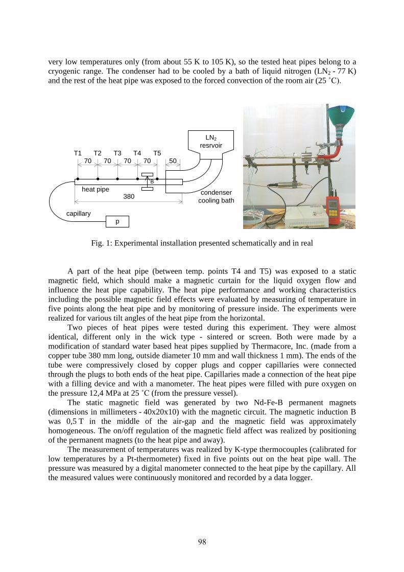
very low temperatures only (from about 55 K to 105 K), so the tested heat pipes belong to a

cryogenic range. The condenser had to be cooled by a bath of liquid nitrogen (LN2 - 77 K)

and the rest of the heat pipe was exposed to the forced convection of the room air (25 ˚C).

70 70 70 70 50

380

p

T1 T2 T3 T4 T5

B

heat pipe

LN2

resrvoir

condenser

cooling bath

capillary

Fig. 1: Experimental installation presented schematically and in real

A part of the heat pipe (between temp. points T4 and T5) was exposed to a static

magnetic field, which should make a magnetic curtain for the liquid oxygen flow and

influence the heat pipe capability. The heat pipe performance and working characteristics

including the possible magnetic field effects were evaluated by measuring of temperature in

five points along the heat pipe and by monitoring of pressure inside. The experiments were

realized for various tilt angles of the heat pipe from the horizontal.

Two pieces of heat pipes were tested during this experiment. They were almost

identical, different only in the wick type - sintered or screen. Both were made by a

modification of standard water based heat pipes supplied by Thermacore, Inc. (made from a

copper tube 380 mm long, outside diameter 10 mm and wall thickness 1 mm). The ends of the

tube were compressively closed by copper plugs and copper capillaries were connected

through the plugs to both ends of the heat pipe. Capillaries made a connection of the heat pipe

with a filling device and with a manometer. The heat pipes were filled with pure oxygen on

the pressure 12,4 MPa at 25 ˚C (from the pressure vessel).

The static magnetic field was generated by two Nd-Fe-B permanent magnets

(dimensions in millimeters - 40x20x10) with the magnetic circuit. The magnetic induction B

was 0,5 T in the middle of the air-gap and the magnetic field was approximately

homogeneous. The on/off regulation of the magnetic field affect was realized by positioning

of the permanent magnets (to the heat pipe and away).

The measurement of temperatures was realized by K-type thermocouples (calibrated for

low temperatures by a Pt-thermometer) fixed in five points out on the heat pipe wall. The

pressure was measured by a digital manometer connected to the heat pipe by the capillary. All

the measured values were continuously monitored and recorded by a data logger.

98

Experimental Results

In the following results of above mentioned experiments are presented. We have

measured working performance of the heat pipes with two types of wick - sintered and screen.

The both tested types were measured at different tilt angles as seen in the Fig. 2. The

following graphs present temperature characteristics measured in five points along the heat

pipe (as seen in the Fig. 1), where the curves going in the graph from top to bottom belong to

points from T1 to T5. On the top of each graph time of magnetic field action is marked.

In the Fig. 3 there are temperature characteristics for the empty heat pipe without any

working fluid. So in this case heat was transported only by thermal conductance of the copper

container and the wick. Of course, no magnetic field action could be observed in this case.

Comparing other graphs with this one contribution of the heat pipe operation can be seen.

In the horizontal position (Fig. 4, 6) the heat pipes operated only partially and they

never became almost isothermal, as typical for the standard heat pipe operation. Their

performance was limited by the insufficient wick operation. And because there was only a

small (or even no one) liquid flow within, the magnetic field could not influence the thermal

capability. However, at the screen type (in the Fig. 6) some small magnetic field action on the

temperature characteristics can be remarked.

0°

+30°

-30°

-90°

Heat pipe

LN2

bath

Fig. 2: Heat pipe positioning Fig. 3: Heat pipe without working fluid

Fig. 4: Horizontal position, sinter wick Fig. 5: Gravity assisted heat pipe, sinter wick

Fig. 6: Horizontal position, screen wick Fig. 7: Gravity assisted heat pipe, screen wick

99

Other situation happened when the heat pipe was tilted down with the angle -30˚

(Fig. 5, 7). Now gravity helped the wick to return the condensate to the evaporator section and

the standard operation mode was started. However, in the sintered one (Fig. 5) insufficiency

of the working fluid caused by a large wick saturation is clearly seen (no isothermal state).

The screen one heat pipe (Fig. 7) worked well in this case and became almost isothermal

without the magnetic field exposition. Now, at the both wick types, the magnetic field

influence on heat transport was significantly ascertained. The most dramatic effect was

observed at the screen type, where the temperature T1 (at the end of the evaporator) varies in

the range of about 110 K in dependence on the magnetic field exposition.

Conclusions

In this paper diagnostic of the special heat pipe control method based on the magnetic

field action is presented. Heat pipes with two types of capillary structures were investigated.

The both tested heat pipes were filled with pure oxygen having excellent magnetic properties,

so important for this control method. The results of the measurement are presented in the text.

We have found out only a poor wick capability at the both tested capillary structures

and thus the heat pipes did not work at an adverse tilt angle. We assume it might be caused by

a limited saturation of the wick and by some poor oxygen parameters which are important for

the wick capability. Also horizontally the wick performance was not reliable. However, the

screen one heat pipe seemed to partially work in this position. The return of the condensate

was sufficient only in the gravity assisted mode.

Unfortunately, because of the partial wick failure the magnetic field control effect could

be investigated only in part. The static magnetic field significantly affected heat flow mainly

in the gravity assisted mode. Heat transport was dramatically restricted in this case and results

of our previous experiments with gravitational heat pipes were verified. Some partial

influence of the magnetic field was observed also in horizontal position at the screen one heat

pipe. In other cases the adverse tilt angle disable the liquid flow in the wick and the magnetic

field could not act on it.

This paper is based on the research program no. MSM 6840770012 “Transdisciplinary

Research in the Area of Biomedical Engineering II” of the CTU in Prague and the student

grant SGS 2011 no. OHK3-015/11 “Magnetic Field Effects on Special Thermal Systems” of

the CTU in Prague.

References

1. Cingroš F., Hron T.: Working Fluid Quantity Effect on Magnetic Field Control of Heat

Pipes, Acta Polytechnica 9 / 2009, Praha 2009.

2. Cingroš F., Hron T., Kuba J.: Magnetic Field Control of Cryogenic Heat Pipes,

Mezinárodní konference ISSE 2009, Brno 2009.

3. Cingroš F., Hron T., Kuba J.: Vliv magnetického pole na transport tepla, Mezinárodní

konference Diagnostika2007, Plzeň 2007.

Authors Ing. Filip Cingroš, Doc. Ing. Jan Kuba, CSc.; Department of Electrotechnology, Faculty of Electrical

Engineering, Czech Technical University in Prague; Technická 2, 166 27 Praha; [email protected],

[email protected].

100

Moisture within transformer insulation system Dončuk J., Mentlík V. – FEE UWB in Pilsen Abstract The purpose of this paper is to review moisture activity within the transformer insulation system. Moisture in the insulation system reduces dielectric strength and accelerates the aging rate of the insulation. Sources of water entering into the transformer insulation are residual moisture, atmospheric water and aging decomposition of cellulose and oil. Dangerous effects of water influence the reliability and serviceability of the power transformer. Monitoring of moisture in oil is a suitable and sufficient diagnostic tool to determine the condition of the transformer insulation. Introduction

The power transformer is one of the key devices in state infrastructure. The insulation system is the most sensitive part of the power transformer. The insulation system oil-paper is, during its operation degraded by operating conditions and other factors. One of the most significant degrading factors is moisture which causes the main degradation of the transformer insulation system. Other degrading factors are, for example; temperature, solid particles and electric field. Oil and paper are mainly influenced by moisture ingress and it could lead to damage of the power transformer. Water contamination

The insulation system of the power transformer is composed of oil and solid components. Part of solid insulation is called thin structure. It is composed of the paper insulation of turns, coils and pressboard barriers. Components of thick structure are for example, spacers and clamping ring. Most of the moisture is stored in thin structure. Water comes into thin structure after a few days or months whereas moisture comes into thick structure after a few years. Negligible content of moisture is stored in thick structure. Thin structure is an accumulator of large volume of moisture. Oil is a water-transferring medium. Moisture, migrating between oil and solid part, depends on oil temperature.

There are three sources of water contamination of the transformer insulation. One of the sources of water contamination is residual moisture of the paper insulation that is caused by poor drying during production. The main source of free water is atmospheric moisture and main ingress is through poor sealing of the transformer. Aging decomposition of the cellulose and oil is another source of water appearing in the transformer insulation. Aging produces substantial content of water at high temperatures and it rapidly reduces the lifetime of the power transformer.

Distribution of moisture in the insulation is non-uniform. The majority of moisture is in solid components of the insulation system and it depends on the structure of the cellulose, temperature and solubility of moisture in the oil. Water amount in turns is significantly lower than in pressboard due to higher temperature. Non-uniform distribution of moisture is also in paper layers and it is caused by high temperature. Outer layers absorb more water than inner layers. Dangerous effect of degradation factors

The content of moisture in oil degrades the transformer insulation. Electrical faults caused by partial discharges can occur in the insulation system due to moisture. Bubbles are

101

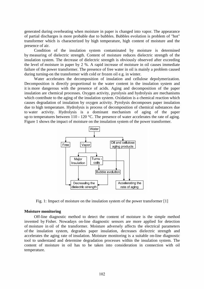
generated during overheating when moisture in paper is changed into vapor. The appearance of partial discharges is more probable due to bubbles. Bubbles evolution is problem of "hot" transformer which is characterized by high temperature, high content of moisture and the presence of air.

Condition of the insulation system contaminated by moisture is determined by measuring of dielectric strength. Content of moisture reduces dielectric strength of the insulation system. The decrease of dielectric strength is obviously observed after exceeding the level of moisture in paper by 2 %. A rapid increase of moisture in oil causes immediate failure of the power transformer. The presence of free water in oil is mainly a problem caused during turning-on the transformer with cold or frozen oil e.g. in winter.

Water accelerates the decomposition of insulation and cellulose depolymerization. Decomposition is directly proportional to the water content in the insulation system and it is more dangerous with the presence of acids. Aging and decomposition of the paper insulation are chemical processes. Oxygen activity, pyrolysis and hydrolysis are mechanisms which contribute to the aging of the insulation system. Oxidation is a chemical reaction which causes degradation of insulation by oxygen activity. Pyrolysis decomposes paper insulation due to high temperature. Hydrolysis is process of decomposition of chemical substances due to water activity. Hydrolysis is a dominant mechanism of aging of the paper up to temperatures between 110 - 120 °C. The presence of water accelerates the rate of aging. Figure 1 shows the impact of moisture on the insulation system of the power transformer.

Fig. 1: Impact of moisture on the insulation system of the power transformer [1] Moisture monitoring

Off-line diagnostic method to detect the content of moisture is the simple method invented by Fisher. Nowadays on-line diagnostic sensors are more applied for detection of moisture in oil of the transformer. Moisture adversely affects the electrical parameters of the insulation system, degrades paper insulation, decreases dielectric strength and accelerates the aging rate of insulation. Moisture monitoring is a suitable on-line diagnostic tool to understand and determine degradation processes within the insulation system. The content of moisture in oil has to be taken into consideration in connection with oil temperature.

102

Moisture is detected by on-line sensors. The majority of moisture sensors are based on the principle of a thin-film capacitive sensor. Electrical properties of the thin-film depend on the content of moisture which is accumulated into this-thin film structure. Capacitance of the thin-film is changed with different content of moisture in oil. The difference of capacitance is measured and it is transferred in moisture in oil in ppm (parts per million).

Moisture in paper is difficult to determine because moisture migrates between oil and paper in dependence of temperature. Sensor for measuring moisture in paper has not been developed yet. The currently used calculation of moisture in paper is reasonable and it is based on the measuring of moisture in oil, oil temperature and the application of the Nielsen diagram. Figure 2 shows Nielsen diagram which represents the dependence of paper moisture on moisture in oil where the temperature of oil is a parameter of this dependence. Moisture in paper is determined in percent of moisture content in the paper insulation.

Fig. 2: Nielsen diagram [3]

Results of moisture monitoring

Fig. 3: Moisture in oil in dependence on temperature

Moisture in oil and oil temperature are measured quantities by sensors in the power transformer. Results shown in fig. 3 represent moisture in oil in dependence on temperature. Moisture capacitive sensor detects higher content of moisture in oil at higher temperatures.

Qv (ppm) - content of moisture in oil

Qvp

(%

) -

cont

ent o

f moi

stur

e in

pap

er

Qv

(ppm

) -

cont

ent o

f moi

stur

e in

oil

Toi

l (°

C)

– te

mpe

ratu

re o

f oil

– temperature – moisture in oil

103

Obtained results confirm theoretical assumptions that majority of moisture is contained in oil at higher temperatures. Assumptions are non-uniform moisture distribution in the insulation system and moisture migration from paper to oil at higher temperatures. Conclusions

This paper has shown that moisture activity influences the insulation system of the power transformer. There are mentioned sources of water entering into the insulation system. Dangerous effects and its impact on the insulation system are presented and shown in fig. 1. A brief principle of moisture sensors operation is described. Moisture in oil in dependence on temperature is shown in fig. 3. Obtained results confirmed assumptions that moisture content in oil is depending on temperature. Further investigation of moisture in paper calculation or measurement is recommended. It would be interesting to compare experiences of moisture in paper calculation with measurement of moisture in oil. Acknowledgement

This article was carried out by the help of Ministry of Education, Youth and Sports of Czech Republic, MSM 4977751310 – Diagnostics of Interactive Processes in Electrical Engineering. References 1. Brochure No. 227 Guidelines for Life Management Techniques for Power Transformers.

CIGRE WG 12.18 Life Management of Transformers, 2002. 125 p. 2. GRIFFIN, P.; SOKOLOV, V.; VANIN, B. Brochure No. 349 Moisture Equilibrium

and Moisture Migration within Transformer Insulation Systems. CIGRE TF A2.30 Moisture in transformer, 2007. 23 p.

3. MENTLÍK, V., et al. Diagnostika elektrických zařízení. Praha: BEN - technická literatura, 2008. 440 p. ISBN 978-80-7300-232-9.

4. PROSR, P., et al. Condition Assessment of Oil Transformer Insulating System. In International Conference on Renewable Energies and Power Quality (ICREPQ’10), Granada (Spain), 23rd to 25th March, 2010, p. 4.

5. POLANSKÝ, R., et al. New Approach in Insulation System of Power Transformers : Insulating Oils with Less Impact on the Environment. In International Conference on Renewable Energies and Power Quality (ICREPQ’10), Granada (Spain), 23rd to 25th March, 2010, p. 4.

6. PUKEL, G.J.; MUHR, H.M.; LICK, W. Transformer diagnostics: Common used and new methods. In International Conference on condition Monitoring and Diagnosis, CMD 2006, Changwon, Korea, April 2006. p. 4.

7. LAKHIANI, VK. Transformer Life Management, Condition Assessment and Dissolved Gas Analysis. Mumbai, Crompton Greaves Ltd, 2006. 160 p.

8. WANG, M.; VANDERMAAR, A. J.; SRIVASTAVA, K. D. Review of Condition Assessment of Power Transformers in Service. IEEE Electrical Insulation Magazine. November/December 2002, Vol. 18, No. 6, s. 12-25.

Authors Ing. Jan Dončuk, prof. Ing. Václav Mentlík, CSc.; Department of Technologies and Measurement, Faculty of Electrical Engineering, University of West Bohemia in Pilsen; Univerzitní 8, 30614 Pilsen; e-mail: [email protected]; [email protected].

104

Radiation Ageing of Flame Retardant XLPE Cables Ďurman V., Lelák J. – FEI SUT Bratislava Abstract The paper discusses the possibilities of using capacitance and tan δ measurements in the range of very low frequencies for investigation of the influence of radiation on the special LOCA cross-linked polyethylene flame retardant cable dielectric. It was found that the measured and calculated parameters depend significantly on the absorbed dose of radiation. The most probable reason of the structural changes in cross-linked polyethylene exposed to radiation is an additional cross-linking. The results also proved that the capacitance measurements in the very low frequency range could be used in practice for estimation of the absorbed dose in polyethylene cables. Introduction

Cross-linked polyethylene (XLPE) is used widely in the cables for transmission and distribution purposes and also for other special applications e.g. in flame retardant cables. Because of its low permittivity and tan δ, XLPE is considered as an efficacious insulating material. Like other materials, it undergoes structural degradation in humid environment. This type of degradation has already been observed and quantified as well as the degradation processes under the electric and the thermal stress [1]. But there are not many results concerning the XLPE behavior influenced by the gamma-irradiation. The radiation can worsen but also enhance the electrical properties of an XLPE dielectric. Research in this field is necessary for the future use of XLPE cables in nuclear power stations. Polymers for the cable applications

Polymer structure comprises long chains consisting of the dipoles with different size and orientation. Each group of dipoles contributes to the relaxation process by a separate part, which appears as a peak in the frequency dependence of the loss factor. The individual relaxation processes are identified by the signs α, β, γ depending on the peak position in the frequency or temperature scale. The α-process belongs to the peak at the lowest frequency (for the constant-temperature measurements) or to the peak at the highest temperature (for the constant-frequency measurements). We can classify the groups of dipoles relative to their placement in the polymer backbone and also according to the type of their motion in an electric field. Two possibilities of a dipole placement toward the backbone exist: parallel and perpendicular. The dipoles, which are not components of the backbone are arbitrary oriented. As for the dipole motion, three possibilities can appear: the localized motion (at the atom level), the segmental motion (at the level of a macromolecule part) and the chain motion (motion of the whole molecule) [2].

Regarding the above classification it was found that the α-process is based on the segmental motion. This type of the dielectric process is a cooperative phenomenon, i.e. the motion of a selected segment influences the neighbor part of the macromolecule and the neighborhood in a feedback influences the original segment. The α-process is caused mostly by the dipoles with perpendicular orientation toward the backbone. The cooperative nature of the α-process has an important consequence: the temperature dependence of its relaxation time does not obey the well-known Arrhenius law but the Vogel-Fulcher-Tammann (VFT) equation. Except of the ordinary α-process, a similar type of relaxation exists in polymers comprising the dipoles with parallel orientation toward the backbone. It is called the normal

105

mode relaxation and it is based on the chain motion. The relaxation frequency of this process appears below the frequency of the α-process.

The second important relaxation process in polymers is the β-process. It is connected with the segmental motion of the dipoles in the side groups. The relaxation frequency of this process is higher comparing with the α-process. The relaxation time obeys the Arrhenius law. The permittivity increment in the complex permittivity functions is less for the β-process than the one for the α-process. The temperature coefficient of the increment is negative for the β-process and positive for the α-process. In relation with the structure of the side groups in polymers, more than one β-process can be recognized in the relaxation spectrum. These processes are then denoted as γ or δ. We can distinguish these processes by their activation energy. The approximate values of energies are 85, 20 and 5 kJ mol-1 for the β- γ- and δ- processes respectively. The degradation degree in power cables during their operation is obviously checked by the dissipation factor (tan δ) measurement. In the time domain the absorption current or recovery voltage can be measured [3]. From these quantities some derived parameters like polarization index are calculated for routine cable evaluation. The parameters acquired by the diagnostic methods mentioned above can individually respond to the changes caused by the long-term operation or to the changes induced by artificial ageing. In this paper the measurements of the complex capacitance and tan δ in the range of very low frequency is used for detecting of the cables degradation caused by irradiation.

Experiment

Specimens of the length 100 cm were cut from a four-core XLPE flame retardant cable and irradiated to get define dose of radiation. Four different doses were chosen (100, 200, 300 and 400 kGy). The source of radiation was a gamma-emitter 60Co with the dose rate of 950 Gy h-1. The irradiated specimens were compared with a non-irradiated specimen from the same cable.

The three cores of each specimen were short connected to create one electrode of the system. The rest core created the second electrode. A complex capacitance of this electrode system was measured in the frequency range 5 mHz - 1 kHz at temperatures from 30 °C to 90 °C by means of the complex capacitance meter build up in our department. The voltage on the specimens during these measurements was 2 V.

Results and discussion

The measured data of capacitance and tan δ are in Figs. 1 - 6.

Fig. 1: Capacitance of non-irradiated cable

with temperature as parameter Fig. 2: Dissipation factor of non-irradiated

cable with temperature as parameter

10-2 10-1 100 101 102 1030

1

2

3

4

5

6

7

6

5

43

2

1

1 - 31 oC2 - 42 oC3 - 50 oC4 - 61 oC5 - 70 oC6 - 80 oC

capa

cita

nce

(10

-9 F

)

frequency (Hz)10-2 10-1 100 101 102 103

0,0

0,2

0,4

0,6

0,8

1,0

1,2

1,4

1,6

6

5432

1 1 - 31 oC2 - 42 oC3 - 50 oC4 - 61 oC5 - 70 oC6 - 80 oC

tan

δ

frequency (Hz)

106

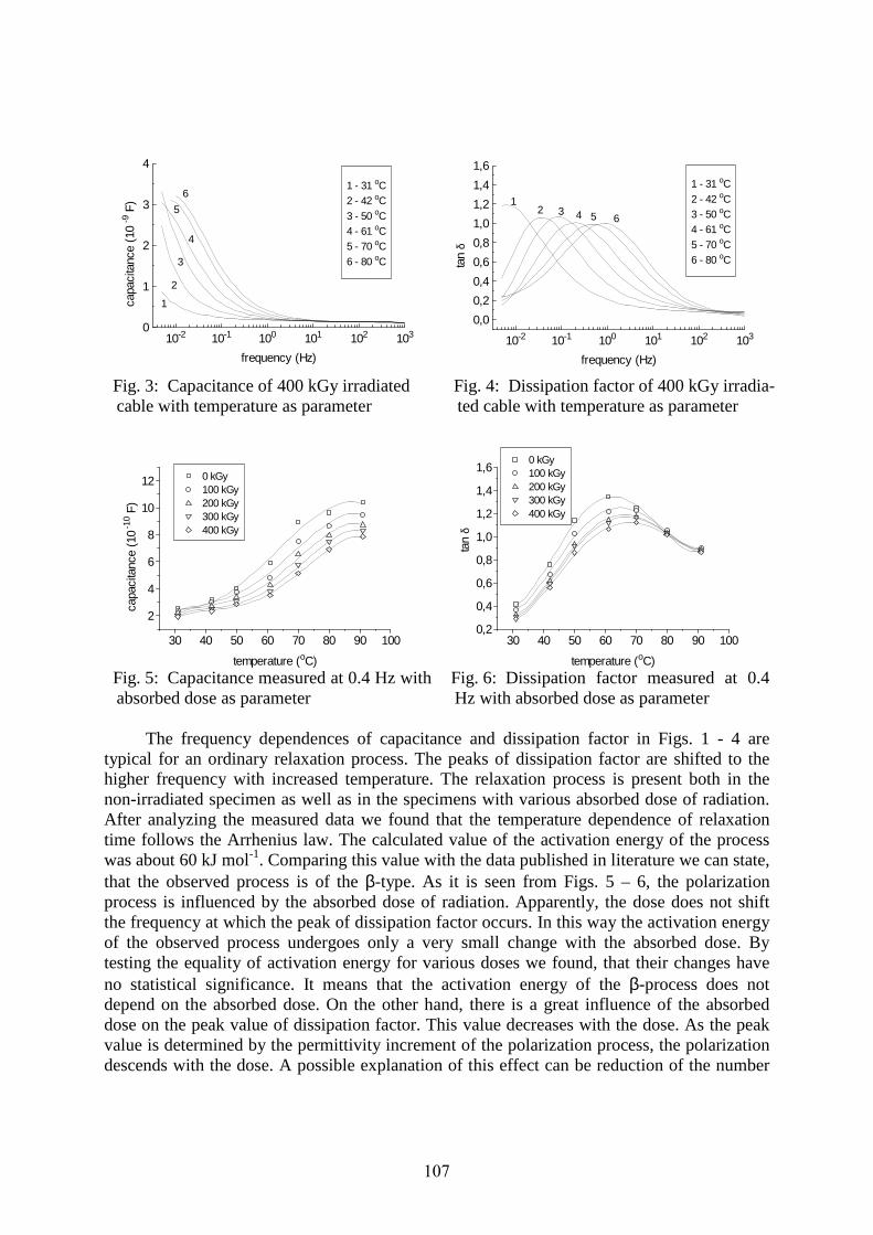
Fig. 3: Capacitance of 400 kGy irradiated

cable with temperature as parameter Fig. 4: Dissipation factor of 400 kGy irradia-

ted cable with temperature as parameter

Fig. 5: Capacitance measured at 0.4 Hz with

absorbed dose as parameter Fig. 6: Dissipation factor measured at 0.4

Hz with absorbed dose as parameter

The frequency dependences of capacitance and dissipation factor in Figs. 1 - 4 are typical for an ordinary relaxation process. The peaks of dissipation factor are shifted to the higher frequency with increased temperature. The relaxation process is present both in the non-irradiated specimen as well as in the specimens with various absorbed dose of radiation. After analyzing the measured data we found that the temperature dependence of relaxation time follows the Arrhenius law. The calculated value of the activation energy of the process was about 60 kJ mol-1. Comparing this value with the data published in literature we can state, that the observed process is of the β-type. As it is seen from Figs. 5 – 6, the polarization process is influenced by the absorbed dose of radiation. Apparently, the dose does not shift the frequency at which the peak of dissipation factor occurs. In this way the activation energy of the observed process undergoes only a very small change with the absorbed dose. By testing the equality of activation energy for various doses we found, that their changes have no statistical significance. It means that the activation energy of the β-process does not depend on the absorbed dose. On the other hand, there is a great influence of the absorbed dose on the peak value of dissipation factor. This value decreases with the dose. As the peak value is determined by the permittivity increment of the polarization process, the polarization descends with the dose. A possible explanation of this effect can be reduction of the number

10-2 10-1 100 101 102 1030

1

2

3

4

6

5

4

3

2

1

1 - 31 oC2 - 42 oC3 - 50 oC4 - 61 oC5 - 70 oC6 - 80 oC

capa

cita

nce

(10

-9 F

)

frequency (Hz)10-2 10-1 100 101 102 103

0,0

0,2

0,4

0,6

0,8

1,0

1,2

1,4

1,6

654321

1 - 31 oC2 - 42 oC3 - 50 oC4 - 61 oC5 - 70 oC6 - 80 oCta

n δ

frequency (Hz)

30 40 50 60 70 80 90 100

2

4

6

8

10

12 0 kGy100 kGy200 kGy300 kGy400 kGy

capa

cita

nce

(10 -1

0 F)

temperature (oC)

30 40 50 60 70 80 90 1000,2

0,4

0,6

0,8

1,0

1,2

1,4

1,60 kGy100 kGy200 kGy300 kGy400 kGy

tan

δ

temperature (oC)

107

of movable dipoles in a unit volume. It is probably a consequence of new bonds created by radiation (cross linking) [4].

Conclusions

The results of our measurements showed that the relaxation process of the β-type is present in the XLPE cable already in the initial state. The radiation weakens the process in such a way, that the number of movable dipoles decreases probably as a consequence of an additional cross-linking of the polymer chains. The change of polarization during the radiation ageing is not dangerous for insulation, as the polarization maximum is far from the cables service frequency. In addition, the peak value of dissipation factor decreases with the absorbed dose. Anyway, the dissipation factor is a good indicator of ageing and also a diagnostic tool. The results proved that the dielectric measurements in the very low frequency range could be used for estimation of the absorbed dose in the cross-linked polyethylene cables subjected to the radiation stress.

Relative higher value of dissipation factor is probably caused by the presence of flame inhibitors in cable insulation.

Acknowledgments

This work has been supported by Scientific Grant Agency of the Ministry of Education of Slovak Republic and the Slovak Academy of Sciences under the project VEGA No. 1/0445/10 and Project: “Increase of Power Safety of the Slovak Republic” (ITMS: 26220220077) supported by the Research & Development Operational Programme funded by the ERDF.

SUPPORTING THE RESEARCH IN SLOVAKIA.

THE PROJECT IS CO-FINANCED BY EU FUNDS.

References 1. Scarpa, P. C. N., Svatik, A., Das-Gupta, K.: Dielectric Spectroscopy of Polyethylene in

the Frequency Range of 10-5 Hz to 106 Hz, Polymer Engineering and Science, 36 No. 8 (1996), 1072-1080.

2. Schönhals, A.: Dielectric Spectroscopy on the Dynamics of Amorphous Polymeric Systems, Novocontrol Application Notes, No.1 (1998), 1-16.

3. Zaengl, W. S.: Dielectric Spectroscopy in Time and Frequency Domain for HV Power Equipment, In: 12th Internat. Symposium on High Voltage Engineering - ISH 2001, Bangalore, India, 20 - 24 August 2001, 1-10.

4. Suljovrujic, E., Stamboliev, G., Kostoski, D.: Dielectric Relaxation Study of Gamma Irradiated Oriented Low-Density Polyethylene, Radiation Physics and Chemistry 66 (2003), 149–154.

Authors Ing. Vladimír Ďurman, PhD., Assoc. Prof. Jaroslav Lelák, PhD; Institute of Power and Applied Electrical Engineering, Faculty of Electrical Engineering and Information Technology, Slovak University of Technology Bratislava, Slovak Republic; e-mail: [email protected], [email protected].

108

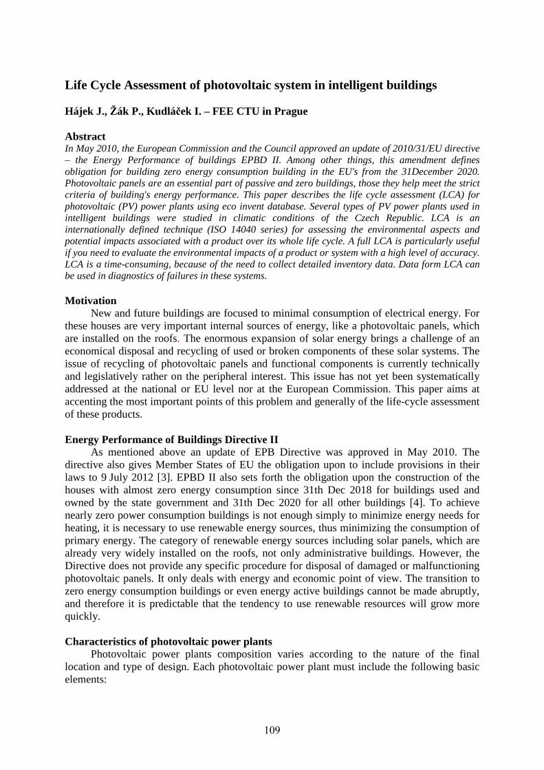
Life Cycle Assessment of photovoltaic system in intelligent buildings Hájek J., Žák P., Kudláček I. – FEE CTU in Prague Abstract In May 2010, the European Commission and the Council approved an update of 2010/31/EU directive – the Energy Performance of buildings EPBD II. Among other things, this amendment defines obligation for building zero energy consumption building in the EU's from the 31December 2020. Photovoltaic panels are an essential part of passive and zero buildings, those they help meet the strict criteria of building's energy performance. This paper describes the life cycle assessment (LCA) for photovoltaic (PV) power plants using eco invent database. Several types of PV power plants used in intelligent buildings were studied in climatic conditions of the Czech Republic. LCA is an internationally defined technique (ISO 14040 series) for assessing the environmental aspects and potential impacts associated with a product over its whole life cycle. A full LCA is particularly useful if you need to evaluate the environmental impacts of a product or system with a high level of accuracy. LCA is a time-consuming, because of the need to collect detailed inventory data. Data form LCA can be used in diagnostics of failures in these systems. Motivation

New and future buildings are focused to minimal consumption of electrical energy. For these houses are very important internal sources of energy, like a photovoltaic panels, which are installed on the roofs. The enormous expansion of solar energy brings a challenge of an economical disposal and recycling of used or broken components of these solar systems. The issue of recycling of photovoltaic panels and functional components is currently technically and legislatively rather on the peripheral interest. This issue has not yet been systematically addressed at the national or EU level nor at the European Commission. This paper aims at accenting the most important points of this problem and generally of the life-cycle assessment of these products.

Energy Performance of Buildings Directive II

As mentioned above an update of EPB Directive was approved in May 2010. The directive also gives Member States of EU the obligation upon to include provisions in their laws to 9 July 2012 [3]. EPBD II also sets forth the obligation upon the construction of the houses with almost zero energy consumption since 31th Dec 2018 for buildings used and owned by the state government and 31th Dec 2020 for all other buildings [4]. To achieve nearly zero power consumption buildings is not enough simply to minimize energy needs for heating, it is necessary to use renewable energy sources, thus minimizing the consumption of primary energy. The category of renewable energy sources including solar panels, which are already very widely installed on the roofs, not only administrative buildings. However, the Directive does not provide any specific procedure for disposal of damaged or malfunctioning photovoltaic panels. It only deals with energy and economic point of view. The transition to zero energy consumption buildings or even energy active buildings cannot be made abruptly, and therefore it is predictable that the tendency to use renewable resources will grow more quickly. Characteristics of photovoltaic power plants

Photovoltaic power plants composition varies according to the nature of the final location and type of design. Each photovoltaic power plant must include the following basic elements:

109

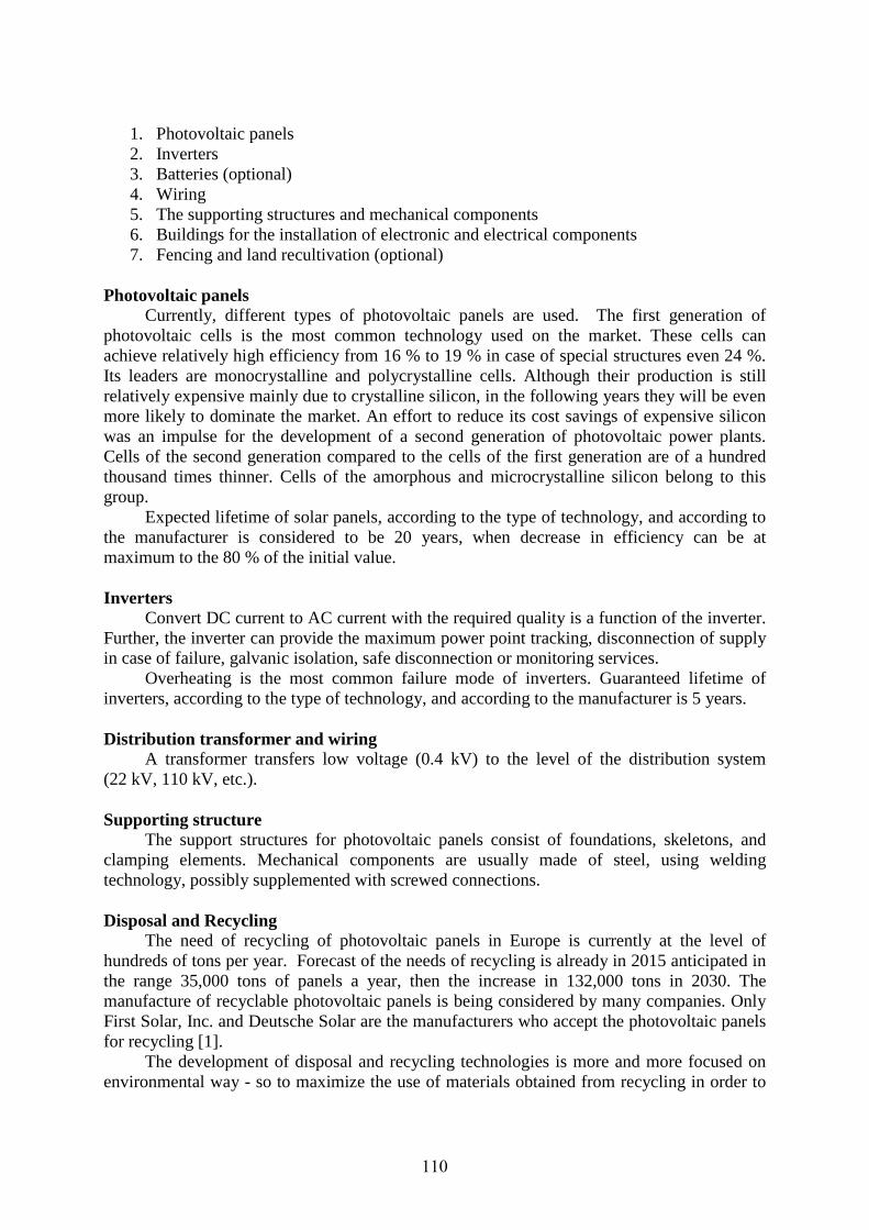
1. Photovoltaic panels 2. Inverters 3. Batteries (optional) 4. Wiring 5. The supporting structures and mechanical components 6. Buildings for the installation of electronic and electrical components 7. Fencing and land recultivation (optional)

Photovoltaic panels

Currently, different types of photovoltaic panels are used. The first generation of photovoltaic cells is the most common technology used on the market. These cells can achieve relatively high efficiency from 16 % to 19 % in case of special structures even 24 %. Its leaders are monocrystalline and polycrystalline cells. Although their production is still relatively expensive mainly due to crystalline silicon, in the following years they will be even more likely to dominate the market. An effort to reduce its cost savings of expensive silicon was an impulse for the development of a second generation of photovoltaic power plants. Cells of the second generation compared to the cells of the first generation are of a hundred thousand times thinner. Cells of the amorphous and microcrystalline silicon belong to this group.

Expected lifetime of solar panels, according to the type of technology, and according to the manufacturer is considered to be 20 years, when decrease in efficiency can be at maximum to the 80 % of the initial value.

Inverters

Convert DC current to AC current with the required quality is a function of the inverter. Further, the inverter can provide the maximum power point tracking, disconnection of supply in case of failure, galvanic isolation, safe disconnection or monitoring services.

Overheating is the most common failure mode of inverters. Guaranteed lifetime of inverters, according to the type of technology, and according to the manufacturer is 5 years.

Distribution transformer and wiring

A transformer transfers low voltage (0.4 kV) to the level of the distribution system (22 kV, 110 kV, etc.). Supporting structure

The support structures for photovoltaic panels consist of foundations, skeletons, and clamping elements. Mechanical components are usually made of steel, using welding technology, possibly supplemented with screwed connections. Disposal and Recycling

The need of recycling of photovoltaic panels in Europe is currently at the level of hundreds of tons per year. Forecast of the needs of recycling is already in 2015 anticipated in the range 35,000 tons of panels a year, then the increase in 132,000 tons in 2030. The manufacture of recyclable photovoltaic panels is being considered by many companies. Only First Solar, Inc. and Deutsche Solar are the manufacturers who accept the photovoltaic panels for recycling [1].

The development of disposal and recycling technologies is more and more focused on environmental way - so to maximize the use of materials obtained from recycling in order to

110

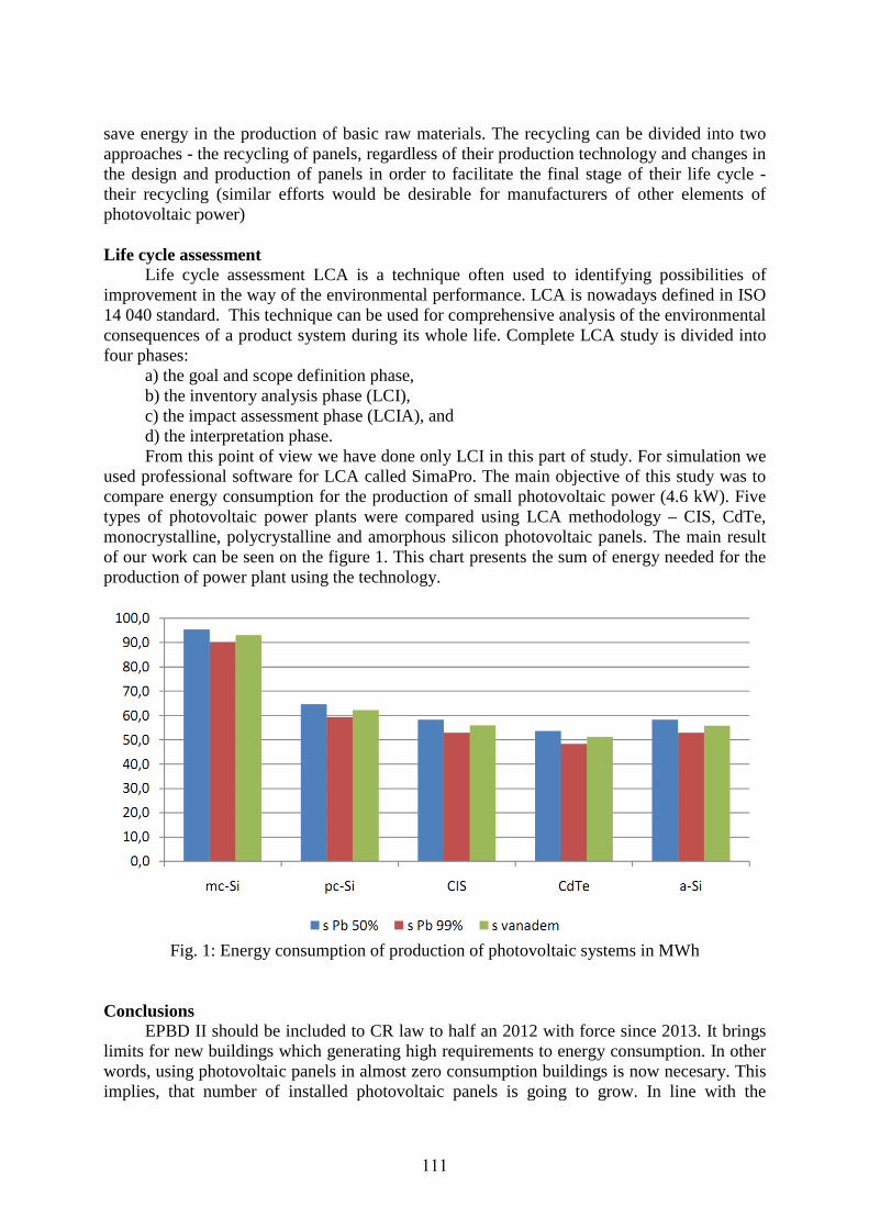
save energy in the production of basic raw materials. The recycling can be divided into two approaches - the recycling of panels, regardless of their production technology and changes in the design and production of panels in order to facilitate the final stage of their life cycle - their recycling (similar efforts would be desirable for manufacturers of other elements of photovoltaic power) Life cycle assessment

Life cycle assessment LCA is a technique often used to identifying possibilities of improvement in the way of the environmental performance. LCA is nowadays defined in ISO 14 040 standard. This technique can be used for comprehensive analysis of the environmental consequences of a product system during its whole life. Complete LCA study is divided into four phases:

a) the goal and scope definition phase, b) the inventory analysis phase (LCI), c) the impact assessment phase (LCIA), and d) the interpretation phase. From this point of view we have done only LCI in this part of study. For simulation we

used professional software for LCA called SimaPro. The main objective of this study was to compare energy consumption for the production of small photovoltaic power (4.6 kW). Five types of photovoltaic power plants were compared using LCA methodology – CIS, CdTe, monocrystalline, polycrystalline and amorphous silicon photovoltaic panels. The main result of our work can be seen on the figure 1. This chart presents the sum of energy needed for the production of power plant using the technology.

Fig. 1: Energy consumption of production of photovoltaic systems in MWh

Conclusions

EPBD II should be included to CR law to half an 2012 with force since 2013. It brings limits for new buildings which generating high requirements to energy consumption. In other words, using photovoltaic panels in almost zero consumption buildings is now necesary. This implies, that number of installed photovoltaic panels is going to grow. In line with the

111

objectives of the European Union, the total installed capacity of solar systems should reach 541 MW in the CR in 2020.

Controlled and legislatively well treated recycling rather than landfilling is the best way to reuse all elements of the photovoltaic power plants. Solar panels contain mainly silicon, whose consumption and thus costs is currently rising quite rapidly. Under the appropriate economic conditions, silver, aluminum and other metals can be reused from photovoltaic systems. The aim is to capture 60 % of panels and recycling them at the level of 80 %. Eg. company First Solar is able to regain 95 % semiconductor and 90 % glass.

The LCA method offers the opportunity to mitigate risks by helping the electronics industry to identify the most environmentally friendly types of photovoltaic technology. The energy consumption is the key criteria in this study. For its calculation we used Cumulative Energy Demand LCA method defined in SimaPro software. The results are presented in the Fig. 1. As you can see, the most energy demanding technology is technology of monocrystalline silicon. Even so monocrystalline photovoltaic panels are much more environmentally friendly comparing to the coal power plants (10,721 tons versus 75,252 tons of CO2-eq.). Compared to the nuclear power plant, the balance is equivalent (11,554 tons CO2-eq.). In terms of energy consumption, CIS technology is the best one, its energy requirements is approximately half (5,237 tons CO2-eq.). Recycling can positively influence energy demands of new photovoltaic systems.

Acknowledgements

This work was supported by the Grant Agency of the Czech Technical University in Prague, grant No. SGS10/163/OHK3/2T/13. References 1. First Solar, Inc., 4050 E. Cotton Center Blvd, Suite 68 Phoenix, AZ 85259 USA 2. ISO 14040. Environmental management – Life Cycle Assessment – Principles and

Framework. 2006. 3. ISSN 1725-2555, doi:10.3000/17252555.L_2010.153.eng 4. Zahradník, P., Novela směrnice EPBD o energetické náročnosti budov 2010/31/EU Authors Bc. Jan Hájek, Ing. Pavel Žák, Doc. Ing. Ivan Kudláček, CSc. ; Department of Electrotechnology, Faculty of Electrical Engineering, Czech Technical University in Prague; Technicka 2, 16627 Prague 6, e-mail: [email protected], [email protected], [email protected].

112

Dielectric Properties of epoxy resins with TiO2 nanofillers

Klampár M., Liedermann K. – FEEC BUT Brno

AbstractThe paper deals with dielectric properties of epoxy resins containing TiO2 nanofiller and with the potential use of dielectric spectroscopy for diagnostics of such nanocomposites. Epoxy nanocomposites are considered as potential insulating materials in transformer stations and parts replacement, as their use may lead to smaller dimensions of the electrical apparatus. Both positive and negative features of TiO2 nanofillers in the epoxy resins are examined. The paper also deals with issues of operation time for these materials. This field of study is of great importance for practical application of epoxy nanocomposites, as the long-time stability of nanocomposites has not yet been established. Just on the contrary, the great number and surface area of interfaces between nanofiller particles and the epoxy matrix itself suggests a larger number of weak points and defect sources, which may contribute to a more rapid deterioration of nanocomposites as compared with classical composites without nanoparticles.

Introduction More stringent requirements on decreasing the dimensions of electrical appliances and

equipment with keeping or even improving their parameters simultaneously result in more exacting requirements at the properties of their electrical insulation. One of such requirements is the need for the replacement of SF6 electrically insulating system in the 66 kV switchgear, possibly even at increasing the operation voltage above this level.

One of the proposed solutions [1], [2] is the replacement of SF6 with the combination of vacuum and solid insulation manufactured from a nanocomposite consisting of an epoxy resin, microparticles and nanoparticles.

Properties of these and analogous systems are currently under intense study. However, owing to a short history of the research and development of nanocomposites, their long-term lifetime and stability remain poorly known [3]. This is particularly annoying, as the lifetime of some of the power engineering applications is expected to be 20 – 30 years. An electrically insulating composite with nanoparticles contains due to its structure a large amount of interfaces, which under a long-term electric field application might act as sources of defects. The objective of our research is the study of electrical properties in the long-term horizon. The long-term aging might be modeled by an accelerated ageing at increased temperatures.

Experimental part The subject of our research are epoxy resins with the admixture of non-conducting TiO2

nanoparticles. Material samples were received from the Institute of Electrical and Electronic Technologies, Faculty of Electrical Engineering and Communication, Brno University of Technology.

Samples were cast in the special casting mold supplied by ABB, Brno. Prior to manufacturing, epoxy resin, hardener, softener and curing accelerator were mixed together in correct shares (by weight). The resulting mixture was stirred and heated to 60 °C, so that the uncured epoxy resin would be thinner and could be better put in the casting mold. The weight of the pure epoxy system is about 350 – 500 g and the share of nanoparticles was set to 5 %. Once nanoparticles are added, they aggregate in the epoxy resin to form nodules, bind air and hence they raise the density of the epoxy resin, which must be degassed. Nanoparticles were admixed and stirred mechanically and by ultrasound for about 30 – 60 minutes. The degassing is followed by the first phase of curing for some 2 to 3 hours at 80 – 90 °C. Once the epoxy resin with nanoparticles added gets rubbery, the casting mold is disassembled, samples are

113

removed, loaded and cured (hardened) in the second phase so as to make them suitable for the three-electrode system. The second phase of curing takes about 10 – 12 hours at 140 °C.

In the nanocomposite manufacture, we used TiO2 nanofiller supplied by Sigma Aldrich. The TiO2 nanofiller were produced by chemical calcinations. Its purity was 99.7 %, the mean value of nanoparticle diameter is around 5 nm and the supplier guarantees that the diameter of nanofiller particle in the powder supplied does not exceed the value of 25 nm.

Dimensions of nanocomposite samples provided were 2.5 mm x 30 mm x 2 mm, i.e., samples were too thick for the purpose of dielectric measurements. Therefore, samples were thinned by grinding them away to the final thickness of 0.41 mm, so that the capacity of the sample reached at least 10 pF. Samples were provided with graphite (or silver) electrodes. Different connections of samples to the measurement system were possible. In the first case samples were inserted into the commercial sample holder HP 16451B. This sample holder was then connected to a standard impedance analyzer HP 4284A with frequency range 20 Hz – 1 MHz.

Fig. 1: HP 16451B sample holder

In the second case samples with painted (or sputtered) electrodes attached to the cold head in the cryostat and each sample was maintained in the thermal contact with the cold head by means of the Apiezon H grease. The task of the Apiezon H grease is to secure a good thermal contact between the cold head and the sample while keeping the cold head and the sample electrically isolated from each other. The applied Apiezon H grease exhibits electrical resistivity of the order 1,2 x 1014 Ωm, so that an electric contact between the cold head Apiezon H grease and the nanocomposite seems to be virtually non-existent. The sample with electrodes was therefore pressed onto the grease and kept in place by an insulating sticky tape (Fig. 2). Outlets from the sample (4-point measurement) were lead to a small rack above the cold head and from there they continued through the body of the cryostat down to the BNC connectors in its bottom part. The BNC connectors were then further lead to the HP 4284A impedance analyzer. The whole measurement, including the temperature control, was PC-controlled.

114

Fig. 2: Overview of the sample attached to the cold head and of the cryostat

A separate part in the measurement of dielectric properties of the epoxy-TiO2

nanocomposites is performing the necessary calibrations and corrections. The HP 4284A impedance analyzer provides three corrections. The first correction is denoted as “Open”, the second one as “Short” and the third one as “Load”. In our measurement, we used only the “Open”, and the “Short” correction. The “Open” correction consists in the adjustment of the distance between the electrodes to such a value, which will be the same as later with the sample inserted between them. The measuring apparatus performs a frequency sweep on the “Open” electrodes, stores the values of impedances obtained during the sweep and thus models the resistance and capacitance of disconnected electrodes. On the contrary, the “Short” correction consists in the short-circuiting of electrodes, so that the electrodes touch each other. After performing the frequency sweep in the same manner as before, the software in the HP 4284A impedance analyzer detects the resistance of connecting wires and afterwards, deducts this value from the measured one, when the sample is inserted between electrodes. Corrections also necessitate setting other parameters, e.g. the length of connection cables. Calibration is performed at the following frequencies: 20 Hz, 100 Hz, 1 kHz, 10 kHz, 100 kHz, 1 MHz and further at 25-, 30-, 40-, 50-, 60- and 80 multiples of these values plus at frequencies 100, 120, 150 multiplied by 101-103. Generally, corrections should minimize the effect of the sample environment upon the measurement results.

Results and discussion Results of the measurement on the nanocomposite sample are shown in Fig. 3.

Fig. 3: Loss number of the nanocomposite sample as a function of frequency at various temperatures

115

Conclusion The observed dielectric spectrum features a single relaxation; the contribution of

electrical conductivity is not visible.In our experiment we intended to compare dielectric properties of a sample without

nanofillers. Unfortunately, the sample without nanoparticles got broken when attempts were made to grind it away to achieve smaller thickness. Hence, the samples could not be compared and, therefore, only the dielectric spectrum of the single nanocomposite sample is presented. Studies on more samples will be necessary so as to exclude a random scatter of dielectric properties.

Acknowledgement This research has been supported by the Grant Agency of the Czech Republic within the

framework of the project GAČR 102/09/H074 "Diagnostics of material defects using the latest defectoscopic methods" and by the Czech Ministry of Education within the framework of MSM 0021630503 Research Intent "MIKROSYN New Trends in Microelectronic System and Nanotechnologies". This support is gratefully acknowledged. We also would like to thank to Mr. Jiří Ovsík for the provision of samples.

References 1. N. Tagami, M. Hyuga, Y. Ohki, T. Tanaka, T. Imai, M. Harada, and M. Ochi, Comparison

of Dielectric Properties between Epoxy Composites with Nanosized Clay Fillers Modified by Primary Amine and Tertiary Amine, IEEE Transactions on Dielectrics and Electrical Insulation, No. 2, 17 (2010), 214-220.

2. N. Tagami, M. Okada, N. Hirai, Y. Ohki, T. Tanaka, T. Imai, M. Harada and M. Ochi, Dielectric Properties of Epoxy/Clay Nanocomposites -Effects of Curing Agent and Clay Dispersion Metod, IEEE Transactions on Dielectrics and Electrical Insulation, No. 1, 15 (2008), 24-32.

3. R. Pfaendner, Nanocomposites: Industrial opportunity or challenge?, Polymer Degradation and Stability, 95 (2010) 369 – 373.

Authorsdoc. Ing. Karel Liedermann, CSc., Ing. Marián Klampár; Department of Physics, Faculty of Electrical Engineering and Communication, Brno University of Technology; Technická 8, 61600 Brno; e-mail: [email protected], [email protected].

116

Design and verification of properties of some components for magnetic

refrigeration near room temperature

Kuba J., Hron T. – FEE CTU in Prague

Abstract A magnetocaloric effect (MCE ) exists in some solid state magnetic materials and can be effective

exploated for refrigeration aimes in the range of near room temperature. In principle MCE can be

characterized as a temperature change ΔT of the material caused by the external magnetic field

modification ΔB under adiabatic conditions or during an isothermal variation with heat supply and

heat sink during the magnetic field variation. The big interest in the refrigeration technology was

enhanced by discovering several materials with “giant” MCE in medium cooling temperature range

without substances harmful for environment. The necessary strong static magnetic field was

generated by the system of two prismatic NdFeB permanent magnets in our case. We namely

engaged with the optimization of the arrangement of magnetic circuit of permanent magnet and pole

shoes for achievement of the maximum induction B of magnetic field round the special gadolinium

heat exchanger (active matrix). Our practical experiences and knowledges concerning of laboratory

experiments at design, manufacturing and testing of the selected components of the developed model

of the magnetic cooling device are written too.

Introduction

A well known magnetocaloric effect (MCE) exists in case of a number of solid state

magnetic materials and can be effective exploated for refrigeration aimes (magnetic cooling)

not only in the range of cryogenic temperatures, but in the range of near room temperatures as

well. In principle MCE can be characterized as a temperature change ΔT of the magnetic

material (active matrix) caused by the external magnetic field modification ΔB under

adiabatic conditions or during an isothermal variation with heat supply and heat sink during

the magnetic field variation. When we will be assume an influence of the external magnetic

field (MF ) with induction B on chosen magnetic material, its magnetization M can be

expressed as

,0

BM

(1)

where χ is magnetic susceptibility of material and μ0 is permeability of vacuum. The changes

ΔB of MF in material induce the changes of its entropy ΔS ( magnetization - demagnetization

) and temperature changes ΔT. For isobaric and adiabatic processes we can express the

MCE by formula

dBMSdT 2 (2)

The change of temperature and amount of the transferred heat depends on the material

composition, absolute temperature, and level of magnetic field induction. The MCE is best

observable in the neighborhood of the magnetic phase transition temperature when a

ferromagnetic material changes into paramagnetic one and vice versa. Up to now, MCE was

widely used in various applications working with low and very low temperatures (for

temperatures below 1 K the method was considered standard). The big interest in the

magnetic cooling technology (MC) was enhanced by discovering several materials with

“giant” MCE in medium cooling temperature range (included the temperature range of near

ambient temperature) without substances harmful for environment. From this point of view

the pure gadolinium Gd and its alloys are the best material available today for MC near room

temperature. The MCE in pure Gd expressed as function ΔT= f(T) at different ΔB is shown

117

in Fig. 1. The MCE of Gd alloys (GdDy, GdTb …) can be considerably stronger. Recent

research on materials showed that exhibit a “giant” MCE , e.g. Gd5 (Si X Ge 1-x )4 , La (Fe X

Si 1-x )13 Hx and MnFeP1-x Asx alloys, are of the most promising substitutes for Ga and its

alloys. For instance the alloy Gd5Si2Ge2 is producing MCE about twice ( 3 to 4 K/T ) that

shown by Gd. The useful operating temperature range of this compound is greater than that of

Gd and it was found that the operating temperature can be tailored from about 30 K to 290 K

by changing the ratio of Si to Ge in the alloy.

Fig. 1: Magnetocaloric effect in gadolinium Fig. 2: Analogy of vapor compression

as function of absolute temperature and magnetic cooling cycle

Magnetic cooling is based on the reversible MCE and for its practical application it is

necessary to realize a series of repeated changes in a certain cycle. Generally, cooling is

achieved by a cyclic magnetization and demagnetization of material. Every cycle consists of

two changes: magnetization and demagnetization (during which heat is either released or

absorbed) and two more changes. The most suitable cycles for moderate cooling are those of

Ericsson and Brayton. Said cycles are predisposed for a good yield of cooling efficiency of

the magnetic materials. An analogy existing between a conventional vapor compression cycle

and magnetic cooling cycle is shown in Fig. 2.

The cyclic magnetizations and demagnetizations of magnetic material may be achieved by its

periodical movement (shift or rotation) inside and outside strong static magnetic field.

Generation of such magnetic fields may advantageously be realized by an appropriate

magnetic circuit excited by permanent magnets (PM). The mentioned system was performed

by two prismatic NdFeB permanent magnets in our case. We namely engaged with the

optimization of the arrangement of magnetic circuit of permanent magnet and pole shoes for

achievement of the maximum induction B of magnetic field in working gap round the special

heat exchanger (active matrix) made from pure Gd. Our practical experiences concerning of

laboratory experiments at design, manufacturing and testing of the selected components of

the developed model of the magnetic cooling device are written in other part of this paper.

118

Design and verification of PM for MC device

Magnetic circuit with permanent magnets for realization of the MC device (in our case)

must contain a working chamber – air gap, where :

magnetic field reaches sufficiently high values and is sufficiently uniform,

allows linear motion of working magnetic material (active matrix).

The starting arrangement of such magnetic circuit with two NdFeB permanent magnets and

pole shoes is in Fig.3. To minimize magnetic leakage the 8 smaller additional PM were used.

Fig.3: The starting PM arrangement for MC device Fig.4: Two heat exchangers with Gd

active matrix in plastic case

An working magnetization space between the pole shoes had dimensions 13/15/60 mm

and are corresponding with real dimensions of Gd active matrix, see Fig.4 (central part of

them). The value of the calculated B was about 1,3 T in the magnetization space. The actual

measured magnetic induction B was lower, about 0,9 T. It means we were focusing to

develop of MF source array to increase the magnetic induction in the working gap. The

second arrangement of magnetic circuit with equal type of NdFeB magnets is shown in Fig.5.

Fig.5: The second arrangement of magnetic Fig.6: The measured curve of B

circuit (2 x PM, 60/60/40 mm) in air gap for z = 0 mm

B (mT)1200

900

600

300

0

Y [mm]0

-30

30

g

Z=0 mm

X [mm]

119

We measured the maximum value of B in air gap about 1 T in this case. In spite of the

fact that we had magnetized permanent magnets, we made attempt to increse of B by

additional magnetization the NdFeB permanent magnets. A special magnetization circuit

with capacitor batery and GTO thyristor was designed and made for that aims. In mentioned

procedure we were using the special transportable hydraulic gauging fixture for short-circuit

of magnetic circuit over the air gap and undirect indication of B changes in the magnetization

space. The volue of B was calculated from adhesive power of gauging fixture in this case. The

experiment shown no signs of incresing of the B. It means that PM was complete magnetized

to maximum during production.

Conclusions

An one from crucial parts of the developed model of the magnetic cooling device is a

source of the strong magnetic field or B in working gap respectively. By our calculations and

laboratory experiments it seams a conventional solution of magnetic circuits with PM is

limited and volume of B in relatively big working air gap is about 1 T. The Halbach

arrangement of PM can be appropriate solution in this case.

Acknowledgements

This paper is based on the research program for students No. SGS11/055/OHK3/1T/13

„Influence of magnetic field on special thermal systems“ of the CTU in Prague.

References

1. Zimm, C., Jastrab, A., Sternberg, A., Pecharsky, V., Gschneidner, Jr. K., Osborne, M.,

Anderson, I.: Description and Performance of a Near-Room Temperature Magnetic

Refrigerator. Advances in Cryogenic Engineering, 43, 1998, pp. 1759–1766.

2. Lee S.J., Kenkel J.M., Pecharsky V.K., Jiles D.C.: Permanent Magnet Array for the

Magnetic Refrigerator, Journal of Applied Physics, vol.91, no. 10, 2002, pp. 8894-8896.

3. Blažková, M.: Magnetické chlazení (Magnetic Cooling). Pokroky matematiky, fyziky a

astronomie. Vol. 50, 2005/4, pp. 301–320 (in Czech).

4. Ota J., Doležel I., Ulrych B.: Study of Suitable Arrangement of Magnetic Circuit with

Permanent Magnets for Realization of Magnetocaloric Effect, in Proceeding of XXXII.

Int.Conf. „SPETO 2009”, Gliwice, Poland, 2009

5. Kuba J., Ota J.: Magnetocaloric Effect in Refrigeration Technology, in Proceedings. of

the International Confrence „Diagnostika 06”, pp. 243-246, ISBN 978-80-7043-557,

Czech Republic, 2006

6. Hron T., Kuba J., Cingroš F.: Magneto Calloric Effect in Gadolinium, 32nd

International

Spring Seminar on Electronics Technology, in Cd proceedings, ISBN 978-80-214-3874-

3, Brno, Czech Republic, 2009.

Authors Doc. Ing. Jan Kuba, CSc., Ing. Tomáš Hron; Department of Electrotechnology, Faculty of Electrical

Engineering, Czech Technical University in Prague; Technicka 2, 16627 Prague 6; e-mail:

[email protected], [email protected].

120

Insulating materials and cryogenic temperatures

Kučerová E., Matějka F., Šebík P., Krpal O. – FEE UWB in Pilsen

Abstract Cryogenic temperatures can significantly affect properties of some materials. Materials processed by

cryogenic temperatures show an improvement especially in mechanical properties, but also

improvement in thermal conductivity and dense microstructure. Effects of extremely low temperatures

are also used in low-voltage electrical components to improve the properties and cables. The aim of

our work is to verify the effect of cryogenic temperatures on electrical materials used in heavy-current

electrical engineering. As samples for this experiment were used cardboard, fibreglass and glass mica

composite. Changes in electrical properties of these materials were monitored after the exposure at

cryogenic temperatures.

Introduction

A method of processing a deep freezer cycle of materials, components and equipment is

known from the first half of the last century. This method concerns with metals and is based

on a change of surface or internal structure of the material caused by low temperatures. The

surface of such material is then harder, more resistant to an abrasion and therefore it has a

longer lifetime. These improvements can be accompanied by an increasing tensile strength,

toughness and stability coupled with the release of residual stresses. Not all materials respond

to the cryogenic processing. The improvements depend on the size of the material and total

time of the cooling cycle. Improved mechanical properties, such as increased resistance

against wear after cryogenic tempering in the range of the lowest temperatures – 192 °C, can

be up to 500 % [1].

The cryogenic processing of parts increases the thermal conductivity, condenses and

compresses the microstructure, reduces the mechanical stress of the material, improves the

operative area, toughness and dimensional stability, provides longer lifetime, lower fatigue,

removes breaking, cracking, etc.

An application can be also in low-voltage electrical engineering. Cryogenically

modified parts and components gain better performance due to reducing contact resistance,

improving conductivity and removing residual stresses. Such modified transformers, relays,

contacts, connectors, hi-fi supply and connecting cables, speakers, components, amplifiers,

printed circuit boards evince significantly better properties and improve sound and image

quality.

The aim of this study was to determine whether it is relevant to study cryogenic

temperatures in relation to insulating materials, especially to determine the influence of one,

two or three-component material that is exposed to low temperature exposure. We focused on

these materials: cardboard, Lamplex FR4, Relanex and Relastik [2]. Temperature cycle was

chosen the same which is used by Cryo-center Kyšice, which realizes low-temperature

exposure to metallic materials and components.

Realization and evaluation of the experiment

The samples for measuring were prepared from fibreglass Lamplex FR4 1,5 mm thick,

Relanex 0,48 mm thick, Relastik 0,3 mm thick and cardboard 0,5 mm thick. The size of all

the samples was 100 mm x 100 mm and measurement frequency was 10. The sample

thickness was measured as well as relative permittivity, tg δ = f (U) for voltage at the range

from U = 500 V to 3 000 V. Also tg δ = f (T) was measured for temperatures from T = 30 °C

121

to T = 185 °C, electrical strength, absorption and resorption. These measurements were made

with a metal electrode system, which was attached in the measured samples with the size of

the inner electrode diameter of 50 mm gap between the electrodes 2 mm and width of the ring

shielding electrodes10 mm. A voltage electrode system electrode with a diameter of 20 mm

and ground electrodes 70 mm diameter in the oil lab was used for measurement of breakdown

voltage at 50 Hz.

The materials were exposed in the freezing temperature cycle environment: the

temperature was decreasing during 10 hours from an ambient temperature 22 °C to minus

184 °C, followed by endurance at this temperature for 24 hours and then the temperature was

increasing again within 10 hours back to a temperature of 22 °C.

Relative permittivity r

After the exposure in the cryogenic temperatures the relative permittivity for fifteen

seconds and one minute polarization index is lower for all the materials. The relative

permittivity for ten minutes and hour polarization index is higher by Relanex and Relastik ,

lower by the cardboard and same by Lamplex FR4, see Table 1.

Table 1: Values of relative permittivity εr of monitored materials

Relative permittivity εr ( - )

15´´/60´´ 1´/10´ 10´/60´ 60´/100´

Lamplex FR4

delivered state 2,4 2,6 1,7 1,2

after exposure 1,7 2,4 1,7 1,2

Cardboard

delivered state 1,7 2,3 1,2 0,9

after exposure 1,7 1,9 0,9 0,8

Relanex

delivered state 2,9 4,6 2,3 1,2

after exposure 2,3 3,8 2,4 1,3

Relastik

delivered state 3,1 4,8 2,5 1,3

after exposure 2,3 4,0 2,8 1,4

Voltage dependence tgδ

After the low temperature exposure the tgδ at voltage = 1600 V (partial discharge

appear in the test structure) is lower than before the exposure. At voltage U = 800 V the tg δ is

lower by Relanex and Relastik and higher by the cardboard and Lamplex FR4 (Fig. 1 to 4).

122

Temperature dependence tgδ

From the measured temperature dependences is obvious that at a temperature of 130 °C

the value of tg δ is increasing due to the exposure in the freezing environment by Lamplex

FR4, Relanex and Relastik. The cardboard is vice versa (Fig. 5 to 8).

Fig. 1: Dependance of loss factor tg δ

on voltage for Lamplex FR4

Fig. 2: Dependance of loss factor tg δ

on voltage for Relanex

Fig. 4: Dependance of loss factor tg δ

on voltage for Relastik

Fig. 5: Dependance of loss factor tg δ

on temperature for Lamplex FR4

Fig. 6: Dependance of loss factor tg δ

on temperature for cardboard

Fig. 3. Dependance of loss factor tg δ

on voltage for cardboard

123

Measurement of absorption and resorption [3]

The values of the constants ARRK found out of linear substitutions of relative absorptive

curves are mentioned in Table 2. This table shows that these values decrease after cryogenic

stress by Lamplex FR4, Relanex and Relastik. The constant ARRK rises by the cardboard.

Table 2: ARRK values for tested materials

ARRK

delivered state after exposure after exposure (%)

Lamplex 0,72584 0,55441 76,4

Cardboard 0,49030 0,58128 118,6

Relanex 0,82141 0,70061 85,3

Relastik 0,84971 0,71245 83,8

Electric strength

The measured values of breakdown voltage of the test materials indicate that cryogenic

temperatures cause a slight increase of electric strength for all tested materials.

Table 3: Electrical strength of materials monitored before and after cryogenic stress

Electric strength Ep (kV/mm)

Lamplex Relanex Relastik Cardboard

delivered state 29,3 88,6 95,6 19,1

after cryo stress 29,4 94,4 103,6 19,8

Increase % 0,3 6,5 8,4 3,6

Conclusion

We can conclude that exposure in the cryogenic temperature, with respect to the initial

status, affects the properties of the tested materials, which are expressed by variations in the

measured values. Effect of given stress differs for a one (cardboard), two (Lamplex) or three-

component (Relanex, Relastik) material (Table 4). A positive value indicates improvement in

monitored properties in %, a negative value indicates deterioration in %.

Fig. 7: Dependance of loss factor tg δ

on temperature for Relanex

Fig. 8: Dependance of loss factor tg δ

on temperature for Relastik

124

Table 4: Summary and evaluation of results obtained for the monitored properties

Material

cardboard Lamplex Relanex Relastik

εr 10´ -17,4 -7,7 -17,4 -16,7

tg δ = f(U) at U = 800 V 8,5 9,7 -18,0 -9,0

tg δ = f(T) at T = 130 °C 6,0 -36,0 -19,7 -11,4

Absorption, resorption ARRK 18,6 -25,6 -14,7 -16,2

Ep 3,6 0,3 6,5 8,4

The table shows that the effect of cryogenic temperatures on dielectric properties of

tested materials can be positive.

Acknowledgement

This work was supported by a research plan of the Ministry of Education and Youth and

Sports of the Czech Republic, MSM 4977751310 "Diagnosis of iterative processes in

electrical engineering."

References

1. CRYO-centrum.cz

2. Výzkumný záměr MSM číslo 49777513110 „Diagnostika interaktivních dějů

v elektrotechnice“.

3. Mentlík V.: Dielektrické prvky a systémy. BEN – technická literatura 2006.

Authors doc. Ing. Eva Kučerová, CSc., Ing. František Matějka, Pavel Šebík, Ing. Ondřej Krpal; Department of

Technologies and Measurement, Faculty of Electrical Engineering, University of West Bohemia in

Pilsen; Univerzitní 8, 306 14 Pilsen; e-mail: [email protected], [email protected],

[email protected].

125

Study on the Effect of Addition of Spherical Silver Nanoparticles into

Electrically Conductive Adhesives

Mach, P. – FEE CTU in Prague

Abstract Electrical resistance and nonlinearity of current vs. voltage characteristic of adhesive joints formed of

electrically conductive adhesives modified with addition of spherical silver nanoparticles are

investigated. The resistance is measured using a four point method, the nonlinearity using a

modulation technique. Measurement of nonlinearity using a very pure sinusoidal current is discussed,

too. The samples are prepared by adhesive assembly of jumpers (resistors with the “zero” resistance)

of the type 1206 on a test board of FR4 covered with a copper foil with the thickness of 40 m.

Contact leads of jumpers have surface finish proper for adhesive assembly. No special surface finish

of pads is used. Adhesive is applied by dispensing, jumpers are placed using a semi-automatic pick

and place machine. The results of the measurement show that addition of spherical silver

nanoparticles into standard adhesive does not improve electrical conductivity of adhesive and

increase nonlinearity of a current vs. voltage characteristic of adhesive joints. The reason is increase

of number of contacts in conductive net in adhesive caused by added nanoparticles.

Introduction

Electrically conductive adhesives (ECA) are materials used for conductive joining in

electronics besides soldering. ECA are composed of two components: of insulating matrix

into which electrically conductive particles of filler are mixed. These particles are mostly

metal flakes with dimensions from 10 to 30 microns for adhesives with isotropic electrical

conductivity. The most frequently used material of flakes is silver. The concentration of filler

in adhesive is between 60 to 80 % b.w. Therefore the price of ECA is comparable with the

price of silver on the market. Other metals, such as gold, palladium or nickel are also used.

Epoxy, silicon or polyamide resin is used as an insulating matrix. The most frequently

used resin is epoxy. Silicon or polyamide resins are used for applications appointed for harder

climatic conditions [1].

With respect to the price of electrically conductive adhesives in comparison with lead-

free solders and with respect to the fact that contemporary electronics is mostly focused at

fabrication of low cost electronics, adhesive assembly is limited for some special applications

only. It is used for assembly of heat sensitive components, which could be damaged with the

temperature used for soldering and for assembly of integrated circuits with fine pitch

packages, where soldering causes bridging of neighbor component leads.

Properties of ECA are worst in comparison with properties of lead free solders. Climatic

resistivity, mechanical properties, stability of parameters, life time and many other parameters

of lead free solders are better. Electrical properties, especially the resistance of adhesive

joints, nonlinearity of these joints and their noise are higher than the same parameters of

soldered joints [2]. Therefore different ways are tested for improvement of these properties.

Addition of nanoparticles into standard adhesive filled with micron flakes is one of many

ways, which should be examined [3].

The paper shows results of a study of the resistance and nonlinearity of adhesive joints

formed of adhesive filled with micro-particles into which a small amount of spherical

nanoparticles is mixed. The method of the measurement of joint resistances as well as the

measurement of nonlinearity of adhesive joints is also presented.

126

Experimental

Samples Preparation

Electrically conductive adhesive used for experiment is of an epoxy type (bis-phenol

epoxy). Electrical conductivity of adhesives is isotropic. Epoxy matrix is filled with silver

flakes in concentration of 75 % b.w.

Three types of spherical nanoparticles are used for modification of adhesives. Diameter

of nanoparticles is 6 – 8 nm, 3 – 55 nm and 80 –

100 nm. Concentration of nanoparticles is 1 %,

3 % and 5 % b.w.

Adhesive joints are formed by assembly of

jumpers of the type 1206 on a test board.

Adhesive is applied by dispensing. Jumpers with

surface finish for adhesive joining are used.

Jumpers are resistors, which should have the

“zero” resistance. The measured resistance of

jumpers is 14 m. The test board is of FR4 plated

with copper foil of the thickness 40 m. The

layout makes the four point measurement

possible. No special surface finish is used for the

pads. The test board with assembled resistors is

shown in Fig. 1, the dimensions of the layout in

Fig. 2 and the structure of an adhesive joint in

Fig. 3.

Measurement

The resistance of adhesive joints is

measured using the four point probe (see Fig. 4).

Five measuring tips are used for the

measurement. They are labeled 1 to 5 in Fig. 4.

The first measurement is carried out in position Y

of the switch S. If it will be assumed that the

resistance between a measuring tip and a jumper

lead (this resistance is in the range of

0,24 to 0,86 m) is so small that it can be

neglected in comparison with the resistance of the

adhesive joint (the joint resistance is in the range

of 10 to 45 m), the measured voltage is:

)(5 JOINTJUMPERTIP RRIU (1)

If the switch S is switched in position X, the measured voltage has the value:

)2(2 JOINTJUMPERTIP RRIU

(2)

Fig. 1: Test board with assembled

jumpers

Fig. 2: Test board dimensions

Fig. 3: Adhesive joint. There is a part of

a component in the left top corner, basic

gray line is Cu. In the middle are silver

flakes of adhesive

127

The resistance of the adhesive joint is:

I

UUR TIPTIP

JOINT52

(3)

Nonlinearity of the current vs. voltage characteristic can be measured by two ways:

using powering of a joint with a very pure sinusoidal current and measuring of third harmonic

of a periodical voltage, which occurs on the joint, or using a modulation technique. The

principle of the modulation technique is as follows:

A nonlinear component is powered with two sinusoidal signals with frequency f1 and f2

(see Fig. 5). Nonlinearity causes origin of intermodulation periodical signals with the

frequency:

21 mfnff (4)

If the third harmonic is examined, then sum of parameters n and m must be equal to 3.

Following frequencies are used: f1 = 150 kHz, n = 2, f2 = 4,1062 MHz, m = 1, and

f = 4,4062 MHz.

Because level of signal, which is measured, is in V, the measuring system must be

carefully screened and grounded. It is necessary to avoid to earth loops.

Measured results and discussion

Measured results are shown in Fig. 6. Nine groups of samples are prepared and

measured – for every concentration of nanoparticles and for every type of nanoparticles.

Twenty eight values are measured for every combination.

Data are processed using mathematical smoothing. The simplest method of

mathematical smoothing is used – two maximum and two minimum values of data measured

for every combination nanoparticle type /concentration are deleted and average is calculated

of 24 values.

It is shown that addition of nanoparticles does not improve electrical conductivity of

adhesive joints. The reason is that nanoparticles do not create additional bridges between

neighboring silver flakes of filler, but they locate between flakes and increase number of

contacts in conductive net in adhesive.

Jumper

I

V

1 2

Layout Adhesive

A B

43

XY

5

S

Adhezive

joint

Spectral

analyzer

Matching

circuit

Crystal

oscillatorFilter

In 1 (4,1062 MHz)

In 2 (150 kHz)

Fig. 4: Resistance measuring using

four point method

Fig.5: Principle of measuring of joint nonlinearity using

modulation technique

128

Electrical conductivity of

a balk is based on a phonon-

electron interaction. The

conductive mechanism in a

contact is based on two

mechanisms: on a restriction

mechanism and on a tunneling.

If flakes are used,

restriction mechanism can be

neglected.

The tunneling mechanism

is usually taken as a dominant

one in contacts between flakes

of ECA filler. The tunneling

resistance is higher in

comparison with the resistance

of balk. Therefore the more is tunneling contacts in the conductive net; the higher is the

resistance of the adhesive joint.

Conclusions

The electrical resistance and nonlinearity of the current vs. voltage characteristic of

adhesive joints formed of electrically conductive adhesive modified with spherical silver

nanoparticles are investigated. It is found that addition of nanoparticles into adhesive does not

improve its electrical properties. The reason is an increase of the number of tunneling contacts

in conductive net in adhesive caused by nanoparticles.

Acknowledgments The authors would like to thank Ministry education, youth and sports (project

"Diagnostics of Materials", no. MSM6840770021) for the financial support.

References

1. Daoquinang Lu, Wong, C.P.: Isotropic Conductive Adhesives Filled with Low-Melting-

Point Alloy Fillers, IEEE Trans. on Electronic Packagning Manuf., Vol 23, No. 3, July

2000, pp. 185-190

2. Luyckx, G., Dreezen, G.: Electrically Conductive Adhesives as Solder Alternative: A

Feasible Chalenge. Materials for information Technology. Springer London, 2005. Pp.

363-375

3. Heimann, M., Lemm, J., Wolter, K-J.: Experimental Investigation of Carbon

Nanotubes/Epoxy Composites for Electronic Applications. Proc. XXXI International

Conference of IMAPS Poland Chapter, Rzeszów – Krasiczyn, 2007, pp. 55 - 61

Author doc. Ing. Pavel Mach, CSc.; Department of Electrotechnology, Faculty of electrical engineering,

Czech Technical University in Prague; Technická 2, 166 27 Praha 6; e-mail: [email protected].

Jo

int re

sis

tan

ce

(m

)

With

out n

ano

Nan

o 80

-100

nm

Nan

o 3-

55 n

m

Nan

o 6-

8 nm

Concentration 5 % b.w.

Concentration 1 % b.w.

Concentration 3 % b.w.

Fig. 6: Joint resistance for different concentrations and

different types of added silver spherical nanoparticles

129

Partial discharges and breakdown voltage diagnostics during thermal aging of insulating materials Pihera J., Mráz P., Haller R., Mentlík V. – FEE UWB in Pilsen Abstract This paper is focused on thermal aging and accompanied partial discharge diagnostics of two mainly used resin rich mica tapes, which are utilized as a part of insulation system of large rotating machines like turbo or hydro generators. The first tested specimen was mica composite material based on glass fibre and epoxy resin and the second one was composite based on PET and epoxy resin as well. The specimens were tested under laboratory conditions. The materials were thermally aged and the changes of its physical and chemical properties were measured and evaluated. For accelerating the aging process different temperature values (170 – 186 °C) were chosen. The aging time was determined for each temperature value. Specimens of tested material were performed and cured as flat plate 100×100 mm. The measuring of these specimens was carrying out by test voltage at special electrode test setup. For comparing the aging process of the investigated material the trends of measured partial discharge (pd) parameters (inception voltage, extinguish voltage, peak charge level) were studied and described in dependence on exposure time, temperature and applied voltage during measurement. Introduction

The operational lifetime of electrical machines is primary influenced by the insulation system quality. The operational lifetime of electrical insulating system is commonly determined, estimated and predicted in terms of accelerated laboratory aging of tested insulating materials. Accelerated aging could be applied as single factor aging like thermal or electrical aging or multiple factor aging as well. During the multiple factor aging all factors take effect together in the same time. Degradation of an insulation system occurs during the accelerated aging. The degradation is related to the physical and chemical changes within material structure. These changes are consequently detectable with physical or chemical test methods.

Partial discharge testing belongs to one of the high applicable test method of insulating materials within electrical machines. This non-destructive test method allows to determine the degradation ratio or homogeneity of insulation.

The investigated mica resin rich composite based on glass fibre and epoxy resin was thermally aged and the changes of its physical- and chemical properties were measured during accelerated aging. Partial discharges (PD) were measured as well. The characteristic parameters according to IEC 20 670 as inception voltage (Ui), extinguish voltage (Ue) and apparent charge level (Qiec) were measured and analyzed.

At first the preliminary thermally aging lifetime curves of tested materials were performed. As a result of these tests the values of aging temperature and aging time for each temperature level could be determined [1]. Two values characterize the preliminary lifetime curve. First value is the maximal temperature; second one is the minimal endurance temperature. Maximal endurance temperature is given by eight hours endurance test. Minimal endurance temperature is given by temperature class and by the material manufacturer who declared lifetime of material for 30 years at this temperature. The eight hours maximal temperature was determined by the fact that the loss factor value was increased rapidly in comparison to the virgin state or according to the visual changes of specimen (deformations, delaminating, bending, deflection etc). The aging time was determined according to the

130

preliminary lifetime curves ([1], fig.1). The aging temperature values are chosen according to the experimentally total duration and cost as well.

Four aging temperature values for glass fibre material (170, 175, 180, 186°C) and for PET material (170, 178, 186, 194°C) were chosen for material accelerated aging (table 1). The aging time was determined for each

Fig. 1: Preliminary lifetime curve TEST PROCEDURE Partial discharge measurement

The pd testing was performedthe measurement of the recommended Ibehaviour in a well known PRPDand cured as flat plate 100×100 mm, located in a special test setstandardized pd test circuit2 realized by a spring and had a constant value at each test.

Fig. 2: PD circuit

The measuring of partial discharges was performed according to the IEC 60270 [requirements with five specimens aged at one particular temperature and time. The following measuring procedure was carried out: The test voltage was increased up to the inception voltage Ui .When the inception voltage was reached this value was stored and the voltage was again increased up to 1,2 Ui decreased stepwise (DU ~ 1 kV) down to the extinguish voltage was measured Then the test voltage was decreased on 20

1 LEMKE PD SMART 2 the noise level was under 3 pC

preliminary lifetime curves ([1], fig.1). The aging temperature values are chosen according to mentally total duration and cost as well.

Four aging temperature values for glass fibre material (170, 175, 180, 186°C) and for PET material (170, 178, 186, 194°C) were chosen for material accelerated aging (table 1). The aging time was determined for each temperature value ([1], fig.1, table 1).

Preliminary lifetime curve Table 1: Aging temperature values and aging times

Partial discharge measurement performed using a commonly available test system

the measurement of the recommended IEC- magnitudes included the desbehaviour in a well known PRPD- pattern. The specimens of tested material were per

00×100 mm, located in a special test setup and measured in a (fig.2, fig.3). The impact force F to the upper electrode was

realized by a spring and had a constant value at each test.

Fig. 3: Test Setup

of partial discharges was performed according to the IEC 60270 [requirements with five specimens aged at one particular temperature and time. The following measuring procedure was carried out: The test voltage was increased up to the inception

.When the inception voltage was reached this value was stored and the voltage was (~14 kV). After 10 minutes at that value the test voltage was kV) down to the extinguish voltage Ue at each step t

was measured Then the test voltage was decreased on 20 % (~ 9 kV) and the same procedure

threshold

Temperature (°C)

Aging time at given temperature (hour)

Glass fibre 186°C 2 4180°C 8 16175°C 48 96170°C 192 288PET 194°C 1 1,5186°C 2 10178°C 24 48170°C 192 288

preliminary lifetime curves ([1], fig.1). The aging temperature values are chosen according to

Four aging temperature values for glass fibre material (170, 175, 180, 186°C) and for PET material (170, 178, 186, 194°C) were chosen for material accelerated aging (table 1).

temperature value ([1], fig.1, table 1).

Aging temperature values and aging times

lable test system1, which allowed magnitudes included the describing of the pd

ens of tested material were performed up and measured in a

(fig.2, fig.3). The impact force F to the upper electrode was

of partial discharges was performed according to the IEC 60270 [3] requirements with five specimens aged at one particular temperature and time. The following measuring procedure was carried out: The test voltage was increased up to the inception

.When the inception voltage was reached this value was stored and the voltage was tes at that value the test voltage was

at each step the value Qiec % (~ 9 kV) and the same procedure

Aging time at given temperature (hour)

4 6 8 10 16 24 32 48 96 144 192 240 288 384 480 600

1,5 2 2,5 3 10 15 20 25 48 72 96 120 288 384 480 600

131

as described was repeated. Because of the statistic evaluation the procedure was repeated 7 times. It was assumed, that the electrical aging during these procedure can be neglected Breakdown voltage measurement

Breakdown voltage was measured according to the IEC 60243-1 [2]. The breakdown occurs between 10 and 20 second after the moment the voltage was applied and linearly increased. The breakdown was detected by a breakdown detector and the value of voltage was stored. For each value of selected aging temperature and time 7 specimens were tested. RESULTS

Partial discharge behaviour The pd behaviour of PET and glass fibre based material shows independent of the aging

process (temperature, time) some significant difference. At low values of electrical intensity3 the measured charge Qiec of glass fibre are significant smaller than those of PET based material (Fig. 4). If the electrical intensity reaches a value of ~25 kV/mm, the measured charge is rapidly increased and exceeds even the value of the PET material. In the same case the PET specimen “started” at higher electrical intensity but with higher values of the measured charge.

Fig. 4: Value Qiec versus electric intensity - results over the whole aging process

(temperature, time) This behaviour is expressed also in the dependencies of the PD inception intensity at

different aging temperature (Fig. 5).

Fig. 5: Inception intensity of Glass and PET at aging temperature 170°C and 186°C

3 For a better generalizing of obtained results the electrical intensity (U/d) was calculated (d => sample thickness)

132

The inception intensity over the aging time at lower aging temperature (170 °C) shows a typical behaviour over the time- after some higher values the inception intensity decreases to a local minimum, but after that increases again (Fig. 5a). It seems to be some structural changes in the material could be occur. At higher aging temperature (186 °C) the inception intensity is more and less constant over the time (Fig. 6b). In both cases the inception intensity is significantly lower for glass fibre materials. It shall be noticed, that the range of the measured values related to the average value in case of PET is much higher (~30 – 50 %) than for glass fibre materials (15 – 25 %).

That means that the manufacturing process for the PET materials should have a larger complexity than the glass fibre insulation. Another question is the possible influence of cumulated internal charges on the aging process. If can be assumed, that the difference between the inception and extinguish intensity is a certain measure for internal cumulated charge, so can be seen, that only in case of PET materials a small change of charge intensity could be measured over the aging time at different aging temperature. At glass fibre materials this difference does not occur.

The typical PRPD- pattern at 14 kV and 170 °C are shown in Fig. 6. At higher aging temperature this pd- behaviour does not change its principal PRPD- characteristic, but their charge values are increasing.

Fig. 6: PRPD- pattern for PET and Glass Fiber at 14 kV Breakdown Voltage Measurement

Breakdown voltage and electric strength results respectively are presented in Fig. 7-9. There are shown average breakdown values for particular aging temperature and time in Fig. 7 for glass and PET material. There are the values of average values for all measured data and the values of ± σ. There is evident the data are in the range of ± σ. This could be represented as the breakdown voltage doesn’t show any aging process within the material during temperature aging. When the weibull probability plot is constructed from the breakdown data the differences are more evident as shown in Fig. 9. These pictures are build according to weibull probability with dependence on aging temperature.

There are shown other results of breakdown voltage in Fig. 8. These pictures follow life-time curves based on breakdown voltage. The construction of these curves is based on measured data and quadratic model calculation for particular breakdown criteria. The criteria is given as follows: Glass material – 90 kV/mm and PET material – 105 kV/mm.

The model is calculated for measured data and extrapolated for class temperature F (155 °C). Comparing the two materials there is evident that PET based material has better breakdown endurance and higher life-time. It is important to realize that the lifetime curve could be affected by “non-aging” process in breakdown data as described above and shown in Fig.7.

133

a) b) Fig. 7: Electric strength according to aging time – - a) Glass; b) PET

a) b)

Fig. 8: Lifetime curve based on breakdown voltage- a) Glass; b) PET

a) b)

Fig. 9: Weibull Probability a) Glass; b) PET

85

90

95

100

105

110

1 10 100 1000

Ele

ctri

c st

ren

gth

(k

V/m

m)

Aging time (hours)

T170 T175

T180 T186

average value _+sigma

_-sigma

80

85

90

95

100

105

110

115

120

1 10 100 1000

Ele

ctri

c st

ren

gth

(k

V/m

m)

Aging time (hours)

T170 T178

T186 T194

average value _+sigma

y = 1E+24e-0,287x

R² = 0,8951

1,E+00

1,E+01

1,E+02

1,E+03

1,E+04

1,E+05

1,E+06

140 150 160 170 180 190

Ho

urs

Aging temperature (°C)

y = 3E+12e-0,135x

R² = 0,9997

1,E+00

1,E+01

1,E+02

1,E+03

1,E+04

140 150 160 170 180 190 200

Ho

urs

Aging temperature (°C)

134

Conclusions There was shown the experiment of aging of two different materials in this article. The

results of measuring the partial discharge and breakdown voltage was described and discussed as well. There was shown the partial discharges are more sensitive to detect the changes within material structure during thermal aging than the breakdown voltage test.

When comparing the materials of the partial discharge and breakdown strength the PET based material has higher values of breakdown strength, lower partial discharges Qiec values and higher inception intensity of partial discharges. When comparing the behavior during aging, the inception intensity especially, the PET based material has significant decrease of the values. Glass based material doesn’t show the evident decrease of inception intensity and the curves are flat during aging.

It was shown that the pd measurement could be more sensitive to detect the changes within material structure during thermal aging than the breakdown voltage test.

The obtained results show that the PET based material is more robust against thermal aging than the glass fibre materials and, therefore, more appropriate for using in the insulation of large rotating machines. For better understanding of aging process further investigation seems to be necessary. Acknowledgements

This research was funded by the Ministry of Education, Youth and Sports of the Czech Republic, MSM 4977751310 – Diagnostics of Interactive Processes in Electrical Engineering. The authors are grateful for the support of this program. References 1. Mentlik, V, at all.: Research Grant MŠMT Czech Republic, MSM 4977751310, Report

2010. 2. IEC 60 243-1 “Electrical strength of insulating materials - Test methods - Part 1: Tests at

power frequencies”. 3. IEC 60 270 “High-voltage test techniques - Partial discharge measurements”. 4. Bezdekovsky, J., Krupauer, P. Statistical methods for appraisal of quality of stator

winding insulation of big rotating machines , Electroscope, url: www.electroscope.zcu.cz, volume 2009, Number 1, last accessed: January 2011.

5. IEEE 1434-2000: IEEE Trial-Use Guide to the Measurement of Partial Discharges in Rotating Machinery.

6. Hudon, C., Belec, M. “Partial discharge signal interpretation for generator diagnostics” in: IEEE Transactions on Dielectrics and Electrical Insulation, April 2005, Volume: 12 , Issue: 2, pages: 297-319.

Authors Ing. Josef Pihera, Ph.D., Ing. Petr Mráz, prof. Ing. Václav Mentlík, CSc.; Department of Technologies and Measurement, Faculty of electrical Engineering, University of West Bohemia in Pilsen; Univerzitní 8, 306 14 Pilsen; e-mail: [email protected], [email protected], [email protected]. prof. dr. Ing. Rainer Haller, DrSc.; Department of Electric power engineering and Ecology, Faculty of electrical Engineering, University of West Bohemia in Pilsen; Univerzitní 8, 306 14 Pilsen; e-mail: [email protected].

135

Diagnostic system for cable insulation materials

Pinkerová, M., Mentlík, V. – FEE UWB in Pilsen

Abstract This paper is focused on comparing insulation properties of two elastomeric compounds used in cable

industry as a cable insulation. Both insulation materials are based on EPDM rubber (ethylene

propylene diene monomer). The diagnostic system including electrical measurements such as

polarization and depolarization current measurement and measurement of relative permittivity and

dissipation factor is described. Statistical and graphic evaluation of both materials is shown.

Parameters used for comparison are polarization index, insulation resistance, volume resistivity,

dissipation factor and relative permittivity.

Introduction

Diagnostic system is a set of exactly defined procedures; it is possible to describe an

insulation state of each material thanks to the diagnostic system. In this case, the diagnostic

system is the set of measuring, counting and statistical methods. The result of this paper is a

choice from two measured insulation materials by evaluation of obtained values. The chosen

material would have better electrical properties and also it would be better applicable.

The objective of the work was to create the diagnostic system for comparison of

electrical properties of two insulation materials used as cable insulation. The first measured

material consists of silicon rubber, ethylene propylene diene monomer (EPDM) rubber and

additives. The second material consists of mainly EPDM rubber and micro milled mica. The

first one was named K30 and the second one EPDM for this paper.

Monitored parameters

The first step of creating the diagnostic system was to choose electrical parameters

available to comparing insulation materials. Materials would be characterized by insulation

resistance and volume resistivity, dissipation factor and relative permittivity. The polarization

index was selected as additional factor for its good ability to evaluate an insulation state of

material.

Polarization and depolarization current characteristics of materials determine

valuable information about their insulation state [1]. These characteristics represent the

processes, which are proceeding inside the dielectric material, which was inserted between

electrodes of capacitor after switching the direct voltage. The dielectric material is gradually

charged to the stabilised value and the similar situation is coming during its discharging. The

quick change doesn’t occur, the discharging is also gradual. This time variable electrical

charge is shown on the outside by time variable electrical current. Values of this current were

read in the periodically intervals during measurement. Additional characteristic parameters

were next calculated from obtained data.

Minute polarization index is polarization current in 15th

second divided by

polarization current in 60th

second (1st minute) after connection the direct voltage to the

sample (equation 1). Dry and undamaged materials have values of minute polarization index

greatly higher than 1. Other way round the materials with moist or damaged insulation have

calculated values of polarization index near to 1. It depends on amount of free charge carriers

in the measured material.

pi

ii1

15

60

, [ - ] (1)

136

Insulation resistance of the measuring sample is defined as the ratio of direct voltage

which is connected to the testing electrodes contacting measured sample and total current in

the certain time after connection voltage (equation 2).

I

UR ss

i , [] (2)

Volume resistivity expresses ratio of intensity of direct electric field and current

density inside the measured material. In this paper the volume resistivity were calculated

according to equation 3. iR represents the insulation resistance, A an area of electrode and

h a distance between electrodes.

h

ARiv , [m] (3)

Relative permittivity describes behaviour of insulation materials in the electric field –

their ability to polarize itself. It is defined as ratio of the amount of electrical energy stored in

a material by an applied voltage, relative to that stored in a vacuum.

0C

Cx

r , [ - ] (4)

Dissipation factor is a key property of insulation materials application. It is important

for insulation material how much energy changes to other type of energy (usually unwanted

heat energy) during electric stress. This changed energy is named as dielectric losses. The

point of the energy change is effects occurred in the material structure while the material is

subjected to the electric field. The insulation material is heating because of these effects and it

is necessary to ensure a drain of this heat. Or else it is danger to overheating of the material

and consequently its thermal breakdown. It would represent a loss of insulation abilities.

Dielectric losses are expressed by dissipation factor – tan δ. For good insulation materials the

tan δ is much smaller than 10-2

.

Applied methods

Measuring methods were selected according to the dimension possibilities of testing

samples. Statistical methods were used for evaluation of obtained data and thanks to them it

can easily assess (from variation coefficients) whether the measured data are reproducibly

enough.

Polarization and depolarization current measurement

The measurements were taken by classic Volt-Ampere method (the scheme is shown in

the [1]). This method needs a sufficiently stable voltage source. The voltage source Keithley

240 A and voltage level 500 V was applied. The electric current flowing through the sample

was measured by Keithley 610 C, its measuring range is up to 10-16

A.

Measuring system was put in an aluminium box, which represents shielding from ambient

interfering effects. The shielding was used with aim to measure the most accurate values as is

possible. Ten testing samples from both materials were randomly selected for polarization and

depolarization current measuring. The values of polarization current were read in 15th

, 30th

and 60th

second, next in 2nd

,3rd

, 4th

, 5th

,6th

, 8th

, 10th

, 15th

, 20th

, 25th

and 30th

minute as you can

see in the first table. In this moment the voltage source was unconnected and the measuring

process was repeated at the same way for depolarization current, but only to 5th

minute

(because depolarization is shorter than polarization effect). Obtained data of each sample were

plotted to the graph (Fig. 1).

137

U = 500 V

Ri= 2,27·1013

Ω

ρv= 2,89·1014

Ω.m

pi1= 1,77

Fig. 1: Polarization and depolarization current of sample K30_A7

Measuring of relative permittivity and dissipation factor

The most widely used method for measuring dissipation factor and relative permittivity

in a diagnostics is a Schering Bridge. For these measurements was used PC-based measuring

system LDV-5; it is a product of Lemke Diagnostics GmbH. The principles of classic

Schering Bridge and this system are described in [1]. Next used equipment was three-

electrode system Tettex 2914 YY and voltage source KPB INTRA VDO 38.

The dissipation factor and the relative permittivity were measured on all samples of

both materials (30 samples from material K30 and 30 samples from material EPDM. Average,

median, standard deviation and variation coefficient were calculated from obtained data. They

are shown in table 1.

Table 1: Values calculated from measuring by LDV-5

tan δ [-] Cx [F] Rx [MΩ] P [W] εr [-]

Average 5,31·10-2

8,79·10-12

19,25 7,40·10-5

4,63

Median 5,29·10-2

8,84·10-12

19,20 7,43·10-5

4,66

Standard deviation 3,06·10-3

2,23·10-13

0,88 5,88·10-6

0,12

Variation coefficient 5,85 % 2,58 % 4,65 % 8,08 % 2,58 %

Obtained data were plotted to graphs, the example of this evaluation you can see in the

Fig. 2. In these graphs, the average value was marked by red line and levels of ( X + ζ),

( X + 2ζ), ( X + 3ζ) up and down from the average line by blue lines, where ζ represents a

standard deviation of measured data.

The standard deviation describes a rate of fluctuation of measuring parameter. All

values in all graphs were depicted in the interval from ( X - 3ζ) to ( X + 3ζ) which means

stabilized measuring process and good compactness of obtained data.

138

Fig. 2: Example of graphic evaluation of tan delta values

Results and discussion

Two measured material were named as K30 (1st compound) and EPDM

(2nd

compound). Final comparison is in the table 3. The EPDM compound has better all of

measured parameters. The measurement confirmed that EPDM compound has better dielectric

properties.

Both materials show good results from statistical point of view according to variation

coefficient of measured data, which are completed in [2]. So the measured properties are well

reproducible. This also represents good quality of manufacturing, which means homogeneity

of their properties of both materials.

Table 3: Comparison of measuring parameters

parameters K30 EPDM

Ri [Ω] 2,91·1013

7,88·1014

pi1 [-] 1,87 2,56

ρv [Ωm] 3,72·1014

4,61·1015

tg δ [-] 5,31·10-2

3,29·10-2

εr [-] 4,63 1,80

Conclusion

The results from measuring of electrical properties of two elastomeric compounds used

as cable insulation were summarized. The paper describes properties and used measuring

methods. The results confirmed that set diagnostic system for measuring, evaluating and

comparing of parameters was selected well. The output of this work was research report [2]

and certification for new technology in cable manufacture – Innovation of cable sheaths. The

innovation consists of introduction of new material, which has, according to this work, better

properties, for the manufacturing. The material is based on EPDM rubber (ethylene propylene

diene monomer) filled with micromilled mica.

Acknowledgements

This article was carried out by the help of Ministry of Education, Youth and Sports of

Czech Republic, MSM 4977751310 – Diagnostics of Interactive Processes in Electrical

Engineering.

139

References

1. MENTLÍK, V., PIHERA, J., POLANSKÝ, R., PROSR, P., TRNKA, P.: Diagnostika

elektrických zařízení. Praha: BEN - technická literatura, Praha 2008.

2. PINKEROVÁ, M., MENTLÍK, V.: Vlastnosti vybraných plněných kaučukových směsí,

výzkumná zpráva. FEL ZČU v Plzni 2009.

3. MENTLÍK, V.: Dielektrické prvky a systémy. BEN – technická literature, Praha 2006.

4. DAVID, E.; LAMMARE, L.; NGUYEN, D.N. Measurements of

Polarization/Depolarization Currents for Modem Epoxy-Mica Bars in Different

Conditions. Electrical Insulation Conference and Electrical Manufacturing Expo, 22-24

October 2007, Nashville, TN, ISBN 978-1-4244-0446-9, p. 189 - 193.

5. PRABU, R. Raja et al. Electrical Insulation Characteristics of Silicone and EPDM

Polymeric Blends – Part I. IEEE Transactions on Dielectrics and Electrical Insulation,

Vol. 14, No. 5; ISSN 1070-9878, October 2007, p. 1207 – 1214.

Authors Ing. Martina Pinkerová; prof. Ing. Václav Mentlík, CSc.; Department of Technologies and

Measurement, Faculty of Electrical Engineering, University of West Bohemia in Pilsen; Univerzitní 8,

306 14 Pilsen e-mail: [email protected]; [email protected].

140

Dielectric properties of a composite based on epoxy resin Polsterová H. – FEEC BUT Brno Abstract The paper presents results of an experimental research of dielectric properties of a composite. In the composite studied, the matrix is an epoxy resin and the filler is a finely ground mica in different weight contents. Introduction

In electrical engineering, epoxy resins rank among often used materials, due in particular to their excellent electrical, mechanical and thermal properties and also to their easy forming and casting. Their natural properties are often modified by adding various sorts of fillers. Fillers are primarily inorganic fillers in the form of a finely ground powder or tiny flakes of mica or silicate sand. Inorganic powder fillers are mostly ground mica, ground quartz, talc, feldspar, quartz and marble powder and others. Filled materials are used e.g. in the preparation of casting materials for encasing of electrical apparatuses and equipment, especially in power engineering. Experimental

A four-component casting epoxy resin that is used in the ABB Company, Brno, was selected for the matrix. The filler was a finely ground mica MU85F (muscovite) with average grain size 40 µm. The filler share in samples was selected 0, 10, 20 and 30 % (by weight). Higher filler content was not possible because the casting mixture was then too viscous to allow for casting. Casting was carried out by using a steel mould, which allowed to simultaneously prepare 10 samples in the shape of plane parallel plates with dimensions 110 × 110 mm and thickness 2 mm. Prior to casting, mould walls had to be carefully spread with a separator, which in our case was a silicone grease. In order to be able to cast samples, the mixture had to be heated up to 65 °C. Heating the mixture lowered its viscosity and thus the mixing was improved. When adding components of the epoxy resin to the mixture and in the course of subsequent adding the mica filler, a large volume of air got into the mixture, from which the samples were cast. This made necessary a careful evacuation of the mixture prior to casting. After evacuation, the mixture was poured into the pre-heated mould and evacuation was repeated so as to remove any air which might have gotten into the mixture during pouring. The curing process had two stages, first a pre-curing at 90 °C and then final curing at 140 °C for 10 hours. Manufactured samples were put in desiccators with zero relative humidity.

The surface of samples was sufficiently even, smooth and plane parallel, so that it was not necessary to use evaporated electrodes. In the course of measurements, samples were mounted in the three-electrode press-on system Tettex 2904. Measurements of electrical properties were carried out on dried samples at zero relative humidity. The closed space of the measuring capacitor was filled with molecular sieve. The sample was fetched from the desiccator to the measuring capacitor always the day before the measurement. Once the sample was transferred from the desiccator to the measuring capacitor, the temperature in the electrode system was raised for a short time to some 120 °C; in the course of the following night, the temperature was lowered to the value required for the experiment. The experiment was carried out the next day.

141

The samples were measured for the following dielectric properties: relative permittivity and dissipation factor at the frequency 50 Hz, volume resistivity (using megaohmmeter Radiometer IM6) and breakdown strength (using HV test station 200 kV).

Results

Figure 1 and 2 show plots of relative permittivity and dissipation factor as a function of mica filler content. The values presented were measured at 50 Hz. The relative permittivity of the pure epoxy resin is 3.5 and that of the mica filler is 5.5. The value of the relative permittivity of the final composite exhibits a steady increase with increasing filler content, which corresponds to theoretical assumptions.

The plot of the dissipation factor against filler contents also exhibits an increasing trend. In insulators, this effect is undesirable. The dissipation factor of a composite containing filler in the amount of 30 % increased, compared with the pure epoxy resin, by almost an order of magnitude.

Fig. 1: Relative permittivity against filler contents

Fig. 2: Dissipation factor (at 50 Hz) against filler content

Fig. 3: Breakdown strength against filler content

3,4

3,5

3,6

3,7

3,8

3,9

4,0

0 10 20 30

ε r (-

)

Filler content (%)

0,000

0,005

0,010

0,015

0,020

0,025

0 10 20 30

tg δ

(-)

Filler content (%)

14

16

18

20

22

0 10 20 30

Ep

(kV

/mm

)

Filler content (%)

142

A further negative effect is a moderate decrease of volume resistivity with the increasing filler percentage; the pure epoxy resin sample exhibited the value of 2×1014 Ωm, whereas the sample with 30 % filler content exhibited the value of 5×1013 Ωm. A very important property of casting epoxy resins is their electric breakdown strength. The presence of mica filler brings about a very substantial increase of its value as can be observed in Fig. 3.

Graphic plots show average values obtained by repeated measurements. Permittivity

and dissipation factor were measured at 10 samples for each set, electric breakdown strength on 5 samples for each set. Considering the minimum scatter of measured values, both in case of repeated measurements on the same sample and in case of measurements done on different samples belonging to the same set, the issue of statistical evaluation of measurement errors and uncertaintities did not have to be dealt with. Results of the measurements also prove that mica was always well and evenly dispersed in the matrix and, thus, that all samples of the same set exhibit the identical behaviour. Conclusions

The results established show that samples with higher mica content exhibit worse dielectric properties than epoxy resin alone. This is due to the fact that the basic (unfilled) casting epoxy resin is already a high-quality material with a low value of dissipation factor. The positive impact of the filler appears mainly in the values of electric breakdown strength, which show a marked improvement. A matrix with worse dielectric properties is likely to exhibit improved properties with the increased filler content.

Acknowledgements

The work described in this paper was supported by the FEKT-S-11-7 project Materiály a technologie pro elektrotechniku. Its support is gratefully acknowledged.

References 1. Mentlík,V. Dielektrické prvky a systémy. BEN, Praha 2006. ISBN 80-7300-189-6. 2. Polsterová, H., Havlíček, S., Dielektrické vlastnosti kompozitů na bázi reaktoplastů. In

Odborný časopis pre elektrotechniku a energetiku. 2008. 14(mimořádné). p.139-141. ISSN 1335-2547.

Authors Ing. Helena Polsterová, CSc.; Department of Electrotechnology, Faculty of Electrical Engineering and Communication, Brno University of Technology, Technická 10, 616 00 Brno; e-mail: [email protected].

143

Influence of Thermal degradation on Electrical Parameters of Winding Insulating System of Power Transformers Širůček M., Trnka P., Paslavský B. – FEE UWB in Pilsen Abstract This paper is focused on problematic of thermal degradation of insulating systems. This factor has together with electrical, mechanical and chemical stresses negative influences on key parameters of the power transformers. Electrical degradation is caused especially by partial discharges. Therefore measurement of certain parameters and partial discharges of insulating systems help to find faults and improve reliability and working life of the transformers. Experiment was focused on thermal aging of oil - paper insulating system and influence of non-homogenous areas on partial discharge activities. The two insulating liquids were used in the experiment. The first was mineral oil SHELL DIALA DX and the second was environmental friendly oil ENVIROTEMP FR3. Introduction

Power transformers are referred as transformer used between generator and the distribution circuits [5]. Therefore they are important parts of each electricity supply system. Insulating systems of transformers have significant influence on their reliability and working life. Usually power transformers use insulation systems consisted of solid part and liquid insulation. The solid part based on cellulose is represented by a paper (main insulation of windings) and a transformerboard (spacer, winding roller etc.). Liquid insulation is necessary for potential separation and transformer cooling. During transformer operation its insulating system is degraded by different types of stresses (electrical, thermal, chemical and mechanical). The main factor is heating due to losses especially in a magnetic circuit and winding [1]. Stress together with other factors (e.g. oxidation, chemical degradation) causes decomposition of a solid insulation (cellulose) and a liquid itself. If a thermal stress is applied on insulation system for a long time polar and non-polar particles from liquid and cellulose are segregated. The next consequences of thermal aging are oxidation, increase content of moisture and contaminants, chemical adduct (e.g. H20, CH4, C2H6, C2H4) and acid adduct (e.g. petroleum acid, sulphuric acid, sulphurous acid). Deterioration of the system causes significant changes in electric and non-electrics parameters.

Degradation products could be also created by partial discharge (PD) activity and their thermal degradation mechanism within insulation system too. They are created in imperfections areas of insulating system stressed by electrical field. Partial discharges can contain sufficient energy for hydrocarbon strings dissociation causing degradation of insulation. Study of PD activities vs. phase can show a type of irregularities and accurately to determine the causes of the disorder. Therefore PD measurement is one of important diagnostic method. Experiment

Experiment deals with measurements of important electrical parameters of insulating material used in a winding of a power transformer. Tested parameters were Breakdown voltage, Dissipation factor and Resistivity. They provide information about electrical endurance of system, its losses and about level of leakage current within system. Next aim of experiment was to observe changes these electrical parameters due to thermal aging. Two insulating liquids were tested. The first was mineral oil DIALA DX consists of hydrocarbon molecules and the second biologically easily degradable oil FR3 with natural esters. The experiment was divided into three parts.

144

The first part was focused on measurement of the electrical parameters of transformer oil samples. The measurement was done in ČEZ Oil Laboratory for new and thermal aged (3000 h, 90 °C) oils. Breakdown voltage of oils was measured on the end of the experiment after 4000 h thermal aging.

The second part deals with measurement of Dissipation factor and Resistivity according to ČSN IEC 93 and 250. Samples of the oil-paper insulating system at intervals of 25, 50, 125, 225, 500, 1000, 2000, 3000, 4000 h were measured. Ten transformerboards with dimension 100 x 100 x 1 mm were placed in each of the oil.

The last part of the experiment was a study PD activity in the areas with different sizes of not-regularly overlapped insulating material. Irregularities may cause uneven distribution of electric potential and partial discharges occur. The aim of the experiment was to proof that a small irregularity causes a high partial discharge activity and reversely a large imperfection causes only small one. The test sample was a copper bar wrapped by two layers of kraft paper. Four samples were tested in both oils. In the solid insulation were created two types of irregularities. Measured arrangements were symmetrical insulation and not-regularly overlapped insulation with dimension 3-4 mm (Type A) and 1-2 mm (Type B). Ignition voltages (IV ) were measured in each of insulation arrangement 15 times. The next parameter was values of the Apparent charge (Qiec) in 1. and 10. minutes. Measurements were preformed for higher tested voltages too. Its values were approximately 1.25 times higher than IV of the area.

Fig. 1: a) Test set-up, b) Insulation arrangement of sample Results

Table 1 shows parameters for new and thermal aged oils. Mineral oil compared with FR3 achieved better values of tested parameters except Breakdown voltage. Thermal aged oils had parameters significantly changed, especially FR3. Breakdown voltage of mineral oil fell down approximately about 80 % due to degradation. In FR3 oil was decrease in percentages smaller by half (40 %).

Table 1: Electrical parameters of new and thermal aged oils

PARAMETERS

OILS

DIALA DX FR3 New Thermal Aged New Thermal Aged

Breakdown voltage [kV/2,5mm] 48,8 9,96[1] 74,2 43,2[1]

Dissipation factor for 90 °C [% ] 0,056 0,168 1,76 (0,05)[2] 4,499

Resistivity [Ω.m.1010] 279,6 69 0,813 (30,0)[2] 0,345

[1] Measured after 4000 h of thermal aging; [2] Catalogue value [3]

a) b)

145

Samples of oil-paper insulating system had decreasing trend of dissipation factor during thermal aging. The value of dissipation factor depended on time when sufficiently impregnation of samples by the oil occurred. The samples in the FR3 oil were impregnated faster (225 h) than in the mineral oil (500 h). Both oils probably require a certain density, for faster impregnation of the sample. Resistivity of insulating system samples in new mineral oil was 8,58 GΩ.m and in FR3 oil was 1,41 GΩ.m. Resistivity was increasing with time of thermal aging. After 125 h stabilization of in samples impregnated by FR3 oil occurred. Samples in DIALA oil were fluctuating around 6,87 TΩ.m. After 4000 h the resistivity reached values 1,77 TΩ.m (FR3) and 42,2 TΩ.m (Technol).

Fig. 2: Dissipation factor vs. Thermal aging (left), Resistivity vs. Thermal aging (right)

The examples of PD pattern with Type A and B areas are in Fig. 3-4. Between both oils

and insulation arrangements were significant differences. The non-homogenous areas had values of Qiec depend on values of the testing voltage. The Qiec of imperfection areas were in range 5 ÷ 290 pC in DIALA and 10 ÷ 320 pC in FR3. The symmetrical insulation values were approximately 8 ÷ 130 pC in DIALA and 3 ÷ 140 pC in FR3 oil. Average values of IV calculate from all measurement in DIALA and FR3 oils shows Table 2.

Charge [pC]

Charge [pC]

Fig. 3: PD pattern of Type B in DIALA oil – paper insulating system

Fig. 4: PD pattern of Type A in DIALA oil – paper insulating system

0,0E+00

4,0E-02

8,0E-02

1,2E-01

1,6E-01

0 2000 4000

tgδ

[-]

Time of Thermal Aging [h]

Diala

FR3

1,0E+00

4,0E+02

1,6E+05

6,4E+07

2,6E+10

1,0E+13

0 2000 4000

Res

isti

vity

[Ω

.m]

Time of Thermal aging [h]

Diala

FR3

146

Table 2: Average values of IV of tested arrangements

PARAMETER TYPE A TYPE B SYMMETRICAL

DIALA DX FR3 DIALA DX FR3 DIALA DX FR3 Average value

of IV [kV] 0,76 0,72 0,86 1 1,23 1,59

Conclusion

The differences between tested electrical parameters of oil-paper samples impregnated by both thermal aged oils are not as significant as in the case of the liquid itself. Mineral oil has only small changes in electrical parameters during the thermal degradation compared to the FR3 oil.

Dimension of not-overlap areas in both oils have important influence especially on Ignition voltages (IV ). In the symmetrical insulation areas were found the highest values of IV (mineral oil 1,23 kV and FR3 1,59 kV). In areas with imperfection were ignition voltage values significantly lower. Symmetrical areas compared with non-homogenous areas (type A, type B) have higher stability of Apparent charges (Qiec) with higher testing voltages. The discharge activities are especially depending on gaps geometry within the insulation. Therefore is necessary ensuring of suitable drying and winding of insulation sample. Hypothesis that a large imperfection can produce a small discharge activity were confirmed. Acknowledgement

This research was funded by the Ministry of Education, Youth and Sports of the Czech Republic, MSM 4977751310 – Diagnostics of Interactive Processes in Electrical Engineering, Students grant system SGS-2010-037. The authors are grateful for the support of this program. References 1. Mentlik, V.; Trnka, P.; Pihera, J. “Transformer insulation on the threshold of new era.”

In IEEE Electrical Insulation Conference, 2009. Montreal : IEEE, 2009. pp. 129 - 132 . ISBN 978-1-4244-3915-7.

2. Mentlik, V.; Prosr, P.; Trnka, P.; Pihera, J.; Polanský, R. “On-line diagnostics of power transformers.” In Conference record of the 2006 IEEE international symposium on electrical insulation. Toronto : IEEE, 2006. pp. 546-549. ISBN 1-4244-0334-0.

3. Data sheet Cooper Envirotemp FR3 [online], [cit. 2010-01-20], přístupný z WWW: http://www.nttworldwide.com/docs/fr3brochure.pdf .

4. Stockton, D. P., Bland, Jr. J. R., Mcclanahan, T., Wilson, J., Harris, D. L.; Mcshane, P. “Natural ester Transformer fluids: Safety, reliability and environmental performance.“ in IEEE Petroleum and Chemical Industry Technical Conference (PCIC 2007), Canada (Calgary), pp. 1-7. ISBN: 978-1-4244-1140-5.

5. HARLOW, James H. Electric power transformer engineering. USA : CRC Press, 2007. 388 s. ISBN 0-8493-1704-5.

Authors Ing. Martin Širůček, doc, Ing. Pavel Trnka, Ph.D.; Department of Technologies and Measurement, Faculty of Electrical Engineering, University of West Bohemia in Pilsen; Univerzitní 8, 30614 Pilsen; e-mail: [email protected], [email protected]. Ing. Bohumil Paslavský; Department of Electric power engineering and Ecology, Faculty of electrical Engineering, University of West Bohemia in Pilsen; Univerzitní 8, 306 14 Pilsen; e-mail: [email protected]

147

Software for stator bars design, 3D models of stator bars and 3D models of jigs Bezděkovský J., Krupauer P. – BRUSH s.r.o. Plzeň Abstract The target of this project is to automate stator bars design with help of software that has been already made by Stator&Winding Engineering in BRUSH s.r.o.. The target is to simplify a complicated and lengthy creation of bar models and models of all jigs for stator winding. Introduction

In the 2D database program there are inserted the basic parameters of machine (inner/outer diameter, number of slots, number of poles, dimension of slot, length of core etc.). Then other parameters are specified by a designer (cone angle, clearances between endwindings). The program can calculate shapes of endwindings, shape of coils, the winding diagram can be drawn, force between endwindings can be calculated, shape of iron jigs). An AutoCad dxf file can be generated for many views. Then is very easy to finish the drawing and launch the final AutoCad dwg file.

Fig. 1: Diagram of stator winding design

The database program (2D) has been developing in Delphi programming software. New functions and procedures can be added anytime. From Fig. 2 we can see other necessary parameters that define endwinding. It is possible to see the calculated end point of the endwinding.

148

Fig. 2: View of one part of 2D software for stator winding design

Fig. 3 and Fig. 4: The displayed shapes can be saved in dxf file In Fig. 3 it is possible to see a “path” of endwinding for a stator bar. This path is

manually drawn on the cone, the metal forming jig is added on the cone and the copper is formed by hand with a hammer.

It is possible to generate a control MS EXCEL (xls) file. This xls file can control the already prepared 3D model of stator bar created in Autodesk Inventor. The coordinates of a middle fiber is calculated in 2D SW.

149

Fig. 5: View of a middle fibre that is an equidistant to cone; the middle fibre controls the 3D pattern in Autodesk Inventor

Fig. 6: 3D model of stator bar including endwinding

150

Fig. 7: 3D model of endwinding with metal jig; the metal jig is used for forming of the

endwinding; a different jig is used for pressing of main wall insulation applied on endwinding Conclusions

In Brush s.r.o. we can calculate the shape of the stator bar with analytic 2D software. This 2D software has been used for calculation and production of many stator windings. We can say that the 2D software has been verified in praxis. From the 2D shape we are able to display 3D model of stator bar. The central motive is to gain 3D coordinates of the middle fiber form the endwinding path. With the middle fiber we are ale to effectively use the 3D Autodesk Inventor.

For the 3D model we are able to design special metal jigs which are used for shaping of conductor stack. The metal jigs are manufactured on a CNC machine. The input data for the CNC machine are gained from the 3D model Autodesk Inventor. The huge benefit is an absolutely conformity between calculated shape and real shape of the manufactured forming jigs. It means that the quality of the pressed insulation is always secured due to 3D model.

The 3D data gained from 3D model can be used for forming of stator bar in CNC forming machine. In future this CNC forming will enable to substitute the labor consuming hand forming with a hammer. Authors Ing. Jiří Bezděkovský, Ing. Petr Krupauer, Ph.D, Ing. Vladimír Sládek, Bc. Tomáš Birner; Konstrukce statorového vinutí, Brush s.r.o.; Tř. Edvard Beneše 39/564, 301 00 Plzeň; e-mail: [email protected], [email protected], [email protected], [email protected].

151

Issues of flicker noise measurements on power semiconductor devices Hájek J., Papež V. – FEE CTU in Prague Abstract Flicker noise is one of the most important quality indicators of electronic devices. Quality of passive elements is often evaluated according noise level, which is deeply affected by material ageing. Noise measurement can be used for lifetime prediction and probability of failures. Concerning semiconductor devices flicker noise is a criterion of used production technology. Influence of ageing is (contrary of passive devices) not so expressive. However, noise measurement allows to reveal latent defects of diode reverse properties that are unidentified by means of standard in-process inspection. Unlike other standard methods noise measurement requires perfect matching of analyzing circuit and investigated device. Used equipment and method deeply affect results of measurement. Introduction

Noise is a random non-periodical signal generated by a common accidental process. There are two basic types of noise detectable both on passive and active devices: thermal noise and flicker noise. Flicker noise of low-power active electronic devices is the most often studied type of noise. Researches on this field are driven by the need of using low signal and low voltage supply. Then, the ratio between signal and noise level (S/N) is a critical parameter of device’s applicability. Thermal noise

In the case of thermal noise, we are thinking about random current with zero average value but nonzero power. It is caused by thermal diffusion of carriers. These current fluctuations last in order 10-12 s. It can be shown, that the spectrum function of thermal noise is in the range up to 100 GHz constant and continuous. Spectrum function decreases to zero above this range, because the total noise-power must be a finite value. Level of thermal noise depends only on absolute temperature of device (T) and on bandwidth (B), where the noise is investigated. Explicitly, thermal noise-power PN is given by equation:

kTBPN = , (1)

where k is Boltzmann’s constant 1,38·10-23 J/K. Therefore kTB [W] is often used as unit for noise power level. Thermal noise is not interesting from the diagnostics point of view, because it is always present and it is influenced only by temperature [1]. That’s why the following text will be not focused on thermal noise.

Flicker noise

Inhomogenities in material structure are the main causes of flicker (current) noise. These inhomogenities can generate fast and random changes of flowing DC current. Thanks to the step current changes the spectrum density will have decreasing trend from units of Hz up to units of kHz. The level of noise voltage related to frequency band 1 Hz is given by the equation:

( ) 12 −= fIRKfU Nβα

, (2)

where K is a proportional constant and exponents α, β describe measured device (usually α, β = 2). Direct current (I) flows through the measured device (resistance R). There are more types of noise described according their origin related to semiconductor devices [2]. The most

152

important noise (especially for diagnostics of power semiconductor devices) is flicker noise (1/f ). It is connected with the capture of free carries on energy levels in the forbidden gap. The presence of energy levels (traps) is influenced by surface effects, especially with leakage current. Reverse polarization is always necessary condition for creation flicker noise. Techniques of noise measurement Contrary to active electronic devices, it has no sense to measure noise figure on power semiconductor devices. They are used for power conversion, not for signal transmition. It is useful to measure the level of flicker (1/f ) noise. Necessary prerequisites are: suitable polarization of device and separation of noise, impedance matching of analyzer and reasonable frequency range in connection with the origin of noise. Polarization of device

Power devices exhibit huge impedance under reverse bias (102 to 103 MΩ). Therefore a source of polarization voltage has to afford sufficient voltage. Flicker noise is in a common frequency band 12 ffB −= given by the equation:

UKf

fUKdffIRKU

f

f

N 'ln2

121222

1

=== ∫− , (3)

so that it is proportional to polarization voltage. Polarization voltage reaches an order of 102 V to achieve current in order units of nA passing through device. Polarization voltage has to be without ripple component. Voltage source should be low-noise and with minimum internal resistance. Then the source will exhibit lowest thermal noise. Ideal voltage source are galvanic cells. It is suitable to connect in series general 4,5 V or 9 V battery of cell (the second one has higher internal resistance and thermal noise thanks to smaller surface of electrodes). Polarization voltage can be regulated by changing the number of cells. Equivalent circuit

When measuring generated noise signal, the device under test (DUT) can be represented by a current source iN, which is over bridged by the crossing capacity CD and a very small conductivity GD. The capacity of pn junction is voltage-dependent ( 2/1−≈ UCD ) and it is in

order 101 pF or 102 pF (depending on diameter of chip and reverse voltage). For example silicon diodes sized 5 mm in diameter and with reverse voltage 2 kV have capacity 20-30 pF under reverse bias 100 V. Source of noise current iN has also its own internal resistance. However, it cannot be measured anyway. Conductivity GD is temperature-dependent as the reverse volt-ampere characteristic (RVAC) depends on temperature. On

higher temperature reverse current increases, so that noise increases too. Afterwards, it is quite a problem to separate flicker noise and uninteresting generation-recombination noise. Heating process can be done e.g. in a silicon oil. DUT is connected to analyzing circuit (see Fig. 1), which can be substituted by parallel coupling of input resistance RZ, and capacity CM. Reasonable frequency range

From point of view of the frequency spectrum, the generated noise matches the white noise that is filtered by an RC low-pass filter of the 1st order. There exists its cut-off

Fig. 1: Equivalent circuit of DUT and measuring analyzer

153

frequency fc. The spectral function F(f ) has a constant value below this cut-off frequency and it has a course recontouring 1/f above it. Typical real spectral function measured on pn junction is shown on the Fig. 2 (curve marked “RTS”). It is necessary to choose frequency range where the noise will be investigated for measurement optimizing. Measurement should be carried out in frequency range, where the ration S/N is the highest.

While the levels of signal and noise are constant then exists a frequency range where is the ration of S/N constant and frequency independent. From the point of view of a signal evaluation technique, it is advisable to choose a maximum frequency band, because then the

power of the processed signal is maximized. We choose the lower limit of band at frequency where the increasing noise of analyzer doesn’t matter and the S/N ration increases. We are avoiding measurements at lowest frequencies (< 10 Hz), where the signal is distorted by non-linearity of analyzer and where the measurement is too long. An upper limit is chosen at frequency where the level of signals falls down and the available ratio S/N decreases as well. Matching is optimal if the maximal noise power generated by the DUT in the range of the measured frequency band is led to the analyzer. Regarding to equivalent circuit of

DUT (Fig. 1) it is useful to set the input resistance RZ of analyzer as high as it is possible. This simplification is valid only when a RC low-pass filter consisting of capacities and resistors will have its cut-off frequency fm given by the equation:

)(2

/1

MD

zDm CC

RGf

++=

π (4)

higher than the highest frequency of the processed signal. Otherwise, for optimal RZ value equation cm ff = is approximately valid. Principle of measurement

Investigated semiconductor device is polarized by DC voltage source U1 with series resistor R1. This resistor prevent to short out noise current iN through the voltage source U1, which seems to be (for noise signal) a short-circuit. Resistor R1 should be low-noise and its resistivity comparable with DUT’s impedance. Capacity C1 provides galvanic separation between polarizing source and analyzing circuit. No DC signal can pass through this capacitor. RC filter consisting from (C1, C2, R2) works as a high-pass filter and it gives the lowest frequency of noise that can be measured. For current values on Fig. 3 (left) it is about 0,5 Hz. Otherwise, the capacity of measured pn junction CD and resistors R1, R2 in parallel create a low-pass filter with a cut-off frequency about 1,5 kHz. It is impossible to observe noise at higher frequency. Low-noise linear amplifier with a high input resistance is used as a matching circuit between DUT and spectrum analyzer. A source follower with a transistor J-FET J 310 has the input resistance 10 MΩ, voltage gain is near to 1 and a noise figure is from 4 dB to 6 dB. The cut-off frequency fm is approximately 400 Hz (with the chip capacity CD of 30 pF) and roughly matches the cut-off frequency of the measured signal.

1,E-07

1,E-06

1,E-05

1,E-04

1 10 100 1000f (Hz)

F(f) (V/√Hz)

RTS

system noise

Fig. 2: Spectrum of flicker noise (RTS) and system noise of analyzer

154

Dynamic Signal Analyzer HP 35670 is used for measuring and statistic processing of noise voltage. Analyzer should have (for optimal power matching) the highest input resistance. But, there are almost no analyzers with higher input resistance than 1 MΩ except of parametric tube amplifiers. DC separation between analyzer and amplifier is provided by capacity C3. Antiparallel diodes protect signal analyzer against impulse overvoltage that can spread from polarized DUT through capacities C1 and C2.

Fig. 3: Principal diagram of measuring circuit (left), processing by analog technique (right)

Described method assumes analyzing of noise signal by means of dynamic signal analyzer. However, signal can be processed by analog technique (see Fig. 3 right). Let connect amplifier’s output parallel to a set of passive filters. Then we can simply analyze the noise on filter’s output using selective voltmeter or scope. This solution enables to recognize flicker noise of DUT and external disturbing signals. Impulse disturbance does not create an expressive distortion of measured signal when analog processing is used. Analog processing unit has much more bigger dynamic range than digital processing unit.

Besides circuit design, measurement is affected by a lot of external factors. Proper shielding of units processing low-level signal is necessary. Sources of DC voltage (polarization of DUT, supply voltage US) should be without a ripple component; be aware of frequency 50 Hz and its multiples. Outer lighting can cause negative influence on reverse current passing through DUT. Due to photo effect on uncovered silicon surface undesired signals can be reveal especially near 100 Hz and its multiples frequencies.

Conclusions

Article is focused on practical aspects of noise measurement on power semiconductor devices. Described methods are usable first of all in production process, testing and quality control or by prediction of reliability and lifetime of power devices. In comparison with other diagnostic methods, noise measurements are not destructive and are carried out on safety low voltage. Methods described in this article were successfully tested during investigation of unstable RVAC on power diodes [3]. This article was supported by research project MSM 6840770017 Development, safety and reliability of electrical equipments. References 1. Papež V.: Technologie elektronických součástek. ISBN 80-01-00829-0. ČVUT: 1992. 2. Blasquez G.: General aspects of noise phenomena. In: Instabilities in silicon devices.

ISBN 04-44-87944-7. Elsevier Science Publishers: 1986. 3. Hájek J., Kojecký B., Papež V.: Investigation of Flicker Noise in Silicon Diodes under

Reverse Bias. In: ISPS ‘10, ISBN 978-80-01-04602-9. Praha: IET 2010. Authors Ing. Jiří Hájek, Doc. Ing. Václav Papež, CSc.; Department of electrotechnology, Faculty of electrical engineering, CTU in Prague; Technická 2, 166 27 Prague 6; e-mail: [email protected], [email protected]

155

The distribution of voltage on the inductor during surge testing (RSO) J. Lábadi, Z. Křelovec – 1.SERVIS-ENERGO, s.r.o. Abstract The aim of this article is to check the distribution of voltage on the inductor (for example a rotor or a stator coil) during surge testing. The surge testing of motor coils has been used since Feb 1926. The article the principle of surge testing, the reason for surge test, voltage distribution during testing and examples of damaged insulation. The principle of surge testing

If a rapidly increasing current is applied to a coil, voltage will be generated across the coil by the principle of induction. The voltage across the coil is given by:

dt

diLV ⋅= (1)

Where V is the terminal voltage across the coil, L is the coil’s inductance, and di/dt is the time rate of change of current pulse.

The terminal voltage V at the leads of the coil is a summation of the induced voltage created between individual loops in the coil. If the insulation separating adjacent coils is weak and if the induced voltage is higher than the dielectric strength of the weak insulation, an arc will form between the coils. Surge testing equipment is designed to create the induced voltage between adjacent coils and detect the arcing indicative of weak or failing insulation.

The internal capacitor is charged to a known voltage by the power supply. At a specific time, a high voltage switch closes, which transfers the charge from the capacitor through the windings to the coil. If the resistances and loss of the entire circuit are such that the system is underdamped, the charge will be able to flow through the inductor and on to the other side of the capacitor, which will result in an oscillation. This process of oscillation will repeat until the resistances and losses in the circuit completely absorb all of the energy that was originally on the capacitor. The terminal voltage on the coil vs. time gives the surge waveform, which is a record of the changes in damped oscillation. [1] The reason to use surge testing

• simple and quick, easy to use between two operation tests • easy to reach high voltage (for example 30 V p-p) between loops • easy to repeat • numerical evaluation of results (shows the difference between waveforms or EAR)

Voltage distribution during testing

The aim of the experiment is to check the distribution of voltage on the inductor. The output from a surge generator is connected to an inductor and across the inductor we record the waveform voltage between adjacent loops of coil.

These waveforms are measured on the first and the second loop of inductor, on the 10th and the 11th and so forth up to the 67th and the 68th loop – we thus save eight waveforms to compare.

156

This paragraph describes the measuring of the voltage distribution on the inductor. At first, it seems that the voltage distribution between loops is nonlinear, where the maximum value is near the inlet thread and the minimum value is one at the outlet, which is grounded. This is partially true, but the voltage measuring on the tested coil (a rotor pole with 69 loops) showed different results. In figure 1, there are waveforms measured between loops to which the voltage of 1400 V (ca. 20 volts per loop) was applied. Figure 1 shows initial surge shock. In figure 2 the whole waveform (the initial of surge and response) is shown. Figure 3 shows the differences in voltage on all measured loop couples, i.e. the distribution voltage on the inductor.

Fig. 1: Oscilogram of voltage between coil loops – beginning of the waveform

Fig. 2: Oscilogram of voltage between coil loops – the entire waveform

-35

-30

-25

-20

-15

-10

-5

0

5

0 0,2 0,4

U [

V]

t [ms]Voltage between loops 1-2

Voltage between loops 40-41

Voltage between loops 68-69

-40

-30

-20

-10

0

10

20

30

0 0,2 0,4 0,6 0,8 1 1,2 1,4

U [

V]

t [ms]Voltage between loops 1-2

Voltage between loops 40-41

157

Fig. 3: Oscilogram of voltage between coil loops – the entire waveform

Examples of damaged insulations

Figure 4 shows waveforms measured on coil with manually added faults in between coil insulation. The first wave is a waveform with correct response and other ones are with faults in loops.

Fig. 4: Oscilogram with faults

-30,5

-30

-29,5

-29

-28,5

-28

-27,5

-27

-26,5

-26

1-2 10-11 20-21 30-31 40-41 50-51 60-61 68-69

U [

V]

Loops of coil

The distribution of voltage on the inductor

-2500

-2000

-1500

-1000

-500

0

500

1000

1500

2000

0 0,2 0,4 0,6 0,8

U [

V]

t [ms]

Comparison without fault and with fault

Without fault Fault between loops 40-41 Fault between loops 40-42

158

Conclusion After applying surge testing, we found out that the distribution of voltage on the

inductor is nonlinear. But there is little difference between differential loops on the coil. The maximum difference between the edge and the middle of the coil is approximately 2 %. There is no difference in voltage between inlet thread and grounded outlet. Figure 4 shows damage located anywhere on the coil can be easily diagnosed. Surge testing can make the diagnosis of problem on a coil fast with very precise results. Surge testing allows for reaching high voltage between loops without using an additional source of voltage. References 1. John Wilson; CURRENT STATE OF SURGE TESTING INDUCTION MACHINES;

Iris Rotating Machine Conference; June 2003, Santa Monica, CA - Baker Instrument Company

Authors Jiří Lábadi, Ing. Zdeněk Křelovec; 1.SERVIS-ENERGO, s.r.o, Tylova 57a, budova 13, 30100, Plzeň; e-mail: [email protected], [email protected]

159

Seebeck effect of ECA Koblížek V. – FEE CTU in Prague Abstract The paper is focused on the Electrically Conductive Adhesive (ECA) that means to the material used mostly in electronics for surface mounting of microchips on printed circuits boards. With clear plan the author fixated to the unusual ECA property- the thermoelectric behavior. For that purpose the flat thermoelectric couples of five types have been created. The thermoelectric voltage in dependence on the temperature difference between cold and warm end of all these thermocouples was measured. From obtained dependences the thermoelectric (Seebeck) coefficient for every thermocouple has been calculated. Introduction

ECA (Electrically conductive adhesive) is heterogeneous system consists from two parts: very small particles of silver and epoxy resin. The material takes its characteristics properties by means of temperature hardening. Before this process the ECA behaves as paste and is fit for application. After hardening (warming) the ECA behaves as a solid with good electrical conductance. The main sphere of ECA use is in electronics, above all as the soft solder substitution [1], [2]. Electrically conductive adhesives have, except for high electrical conductivity, also good thermal conductance and excellent adhesion to most solid surfaces.

As the author of paper is concerned with the physical properties of ECA - in order to get an idea of theirs other applications, have focused on thermoelectric phenomenon because it takes important position among physical properties. Sample preparation

The thermocouples, that one component part is always ECA, were created on glass fiber reinforced plastic strips with dimension 200x15x2 mm. The second component part was made in the form of strip (Fig. 1) by evaporation of relevant metal or metal alloys using flash method. The ECA strip was applied ordinarily by means of single purpose device. The next step was hardening of the adhesive in the oven at temperature of 150 °C.

Fig. 1: Design of thermocouples

a) Evaporated metal layer (1) on laminate (2) with pasted Ag strip (3) in order to create contact with ECA b) Creating of ECA strip (4).

200

15

1 2 3a)

b) 4

160

ECA specification: Eco Solder AX 20 of producer AMEPOX. Content of Silver particles: 75 % by weight [3].

Metal component parts: CuNi (Constantan), Ni, NiCr, Fe, Ag. These materials have been chosen in accordance with thermoelectric scale so that the thermoelectric coefficient values α were both positive and negative compare with silver. Measuring device and set up

The centre of measuring work place is measuring device which enables the sample connect to measuring circuits, generates the variable temperature difference and also stabilizes the sample on unchangeable position. The design concept of the device is made slightly by Fig. 2.

H

Pt100S

CPl

PE

CM

F

HPl 130

Pt100

Fig. 2: Measuring device H – heating, HPl – heated plate, S – sample, CPl – cooled plate, Pt100 – temperature sensor (platinum resistor 100 Ώ), PE – Peltier cooling elements, F – fan, CM – aluminum cooling module.

The block diagram of measuring work place is shown in Fig.3.

Fig. 3: The arrangement of measuring working place HPl – heated plate, H – heating, M1, M2 – temperature meters, S – sample, TC1, TC2 –temperature controllers, Pt100 – temperature sensor, P1…P4 – Peltier cooling bateries, F – fan, S1, S2 – sources.

161

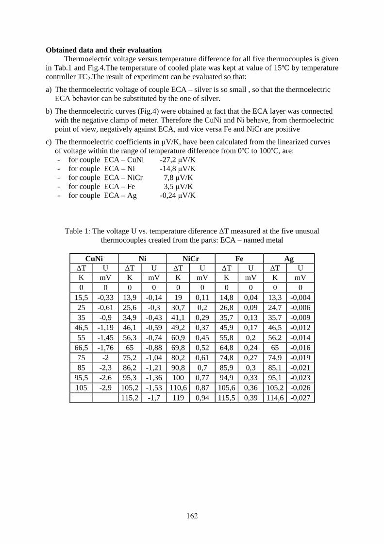
Obtained data and their evaluation Thermoelectric voltage versus temperature difference for all five thermocouples is given

in Tab.1 and Fig.4.The temperature of cooled plate was kept at value of 15ºC by temperature controller TC2.The result of experiment can be evaluated so that:

a) The thermoelectric voltage of couple ECA – silver is so small , so that the thermoelectric ECA behavior can be substituted by the one of silver.

b) The thermoelectric curves (Fig.4) were obtained at fact that the ECA layer was connected with the negative clamp of meter. Therefore the CuNi and Ni behave, from thermoelectric point of view, negatively against ECA, and vice versa Fe and NiCr are positive

c) The thermoelectric coefficients in µV/K, have been calculated from the linearized curves of voltage within the range of temperature difference from 0ºC to 100ºC, are: - for couple ECA – CuNi -27,2 µV/K - for couple ECA – Ni -14,8 µV/K - for couple ECA – NiCr 7,8 µV/K - for couple ECA – Fe 3,5 µV/K - for couple ECA – Ag -0,24 µV/K

Table 1: The voltage U vs. temperature diference ∆T measured at the five unusual thermocouples created from the parts: ECA – named metal

CuNi Ni NiCr Fe Ag

∆T U ∆T U ∆T U ∆T U ∆T U K mV K mV K mV K mV K mV 0 0 0 0 0 0 0 0 0 0

15,5 -0,33 13,9 -0,14 19 0,11 14,8 0,04 13,3 -0,004 25 -0,61 25,6 -0,3 30,7 0,2 26,8 0,09 24,7 -0,006 35 -0,9 34,9 -0,43 41,1 0,29 35,7 0,13 35,7 -0,009

46,5 -1,19 46,1 -0,59 49,2 0,37 45,9 0,17 46,5 -0,012 55 -1,45 56,3 -0,74 60,9 0,45 55,8 0,2 56,2 -0,014

66,5 -1,76 65 -0,88 69,8 0,52 64,8 0,24 65 -0,016 75 -2 75,2 -1,04 80,2 0,61 74,8 0,27 74,9 -0,019 85 -2,3 86,2 -1,21 90,8 0,7 85,9 0,3 85,1 -0,021

95,5 -2,6 95,3 -1,36 100 0,77 94,9 0,33 95,1 -0,023 105 -2,9 105,2 -1,53 110,6 0,87 105,6 0,36 105,2 -0,026

115,2 -1,7 119 0,94 115,5 0,39 114,6 -0,027

162

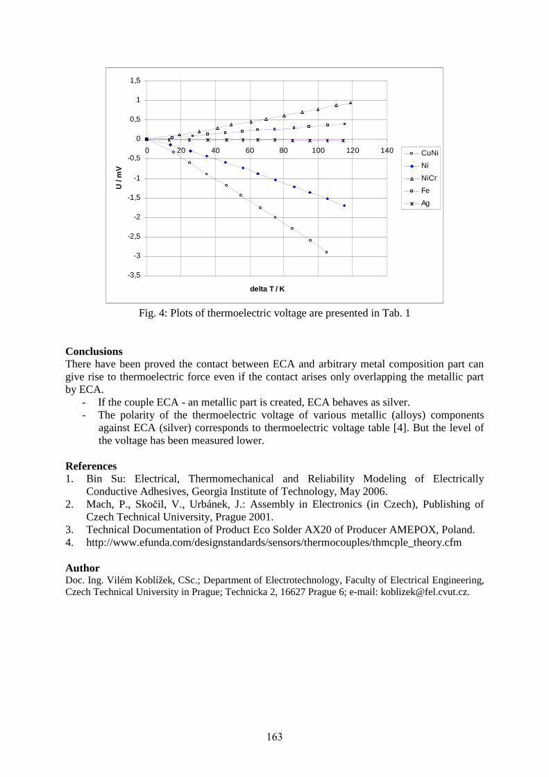
-3,5

-3

-2,5

-2

-1,5

-1

-0,5

0

0,5

1

1,5

0 20 40 60 80 100 120 140

delta T / K

U /

mV

CuNi

Ni

NiCr

Fe

Ag

Fig. 4: Plots of thermoelectric voltage are presented in Tab. 1

Conclusions There have been proved the contact between ECA and arbitrary metal composition part can give rise to thermoelectric force even if the contact arises only overlapping the metallic part by ECA.

- If the couple ECA - an metallic part is created, ECA behaves as silver. - The polarity of the thermoelectric voltage of various metallic (alloys) components

against ECA (silver) corresponds to thermoelectric voltage table [4]. But the level of the voltage has been measured lower.

References 1. Bin Su: Electrical, Thermomechanical and Reliability Modeling of Electrically

Conductive Adhesives, Georgia Institute of Technology, May 2006. 2. Mach, P., Skočil, V., Urbánek, J.: Assembly in Electronics (in Czech), Publishing of

Czech Technical University, Prague 2001. 3. Technical Documentation of Product Eco Solder AX20 of Producer AMEPOX, Poland. 4. http://www.efunda.com/designstandards/sensors/thermocouples/thmcple_theory.cfm Author Doc. Ing. Vilém Koblížek, CSc.; Department of Electrotechnology, Faculty of Electrical Engineering, Czech Technical University in Prague; Technicka 2, 16627 Prague 6; e-mail: [email protected].

163

Diagnostics of electrical equipment as a tool for risk management measures Kopča M., Váry M. – FEI SUT Bratislava Abstract The contribution is devoted to analyzing the effects of early and correct diagnostics of electrical safety status for an objective risk measure in the operation of electrical equipment. Introduction

Electrical equipment accounts for a large group of technical equipment with an increased risk of operation. This is mainly because the electricity they use for their activities by their very nature represents a objective risk to operators and their surroundings. They are mainly the effects of flowing electrical current that is passing through the physiological system and can impair its proper function and cause damage and even death.

Alongside this objective risks resulting from the technical level and the current status of the electrical equipment is in operation of electrical equipment non-negligible in terms of the hazards also the human factor, which is a subjective risk in the operation of electrical equipment.

Despite increasingly stringent measures, it should be noted that the absolute safety of technical equipment is in the technical practice unattainable goal , one can directly say that it is wishful thinking - a myth or a chimera. However, there are tried and tested procedures for the identification, assessment and subsequent risk reduction collectively forming system - risk management system. Risk

The risks, according to the consequences (impact) are usually divided into four groups - categories:

Impact on the individual = individual consequences. Impact on a group of employees = consequences resulting from occupation. Total impact on the public = social consequences. Impact on business, the application of penalties = property damage.

In the literature (economic, security, technical) you can find many definitions of risk, each of which has its typical characteristics, indebted to the field. In practice, the technical definition of risk assessment levels are usually dealing with the effects of unintended consequences in conjunction with the likelihood of such adverse effects may occur. This situation can be described by:

occurance its ofy probabiliteffect unwantedRISK ⋅= (1)

However, the threat is possible to suppress through the introduction of preventive measures. On this basis, perhaps at first sight rather quite simple mathematically definition risk ca be stated as follows:

emeasures)(preventiv protection

(danger)threat RISK = (2)

This definition implies series of risk factors for the practice very important but often underrated and not always correctly applied:

1. Correct identification of risk reduces risk. 2. Risk can be reduced by increasing the effectiveness of preventive measures. 3. It is not possible in technical practice to achieve zero risk.

164

The risk analysis is a process of identification and risk assessment for individuals, property and environment, which are typical for the following activities:

a) Risk identification (detection and description of the risk situation). b) Analysis of the frequency (how often this situation can occur). c) Analysis of the consequences (which may be any consequences).

Basic methods of risk analysis suitable for most technical devices are modified

standard reliability analysis methods (STN IEC 60300-3-1), especially when it comes to specific, so called critical fault, or critical failure state. They are mainly:

1) HAZOP - Hazard and Operability Study. 2) FMEA - Fault Modes and Effect Analysis 3) FMECA - Fault Modes Effects and Critically Analysis. 4) FTA - Fault Tree Analysis 5) ETA - Events Tree Analysis. It is so called black-and white analysis, because it

operates only with trouble-free and faulty state. 6) PHA - Preliminary Hazard Analysis. This type of analysis is inductive, where does the

identification of hazards, hazardous situations and events in an activity that could cause damage or injury. Processes the list of hazards and so called generic (threatening) situations, taking into account the materials used or produced, used equipment, terms of use, spatial distribution and interfaces (links) between elements of the system. It is this method successfully used methods of diagnosis of electrical equipment condition.

7) HRA - Human reliability Assesment. It consists in assessing the impact of operator on systems function in order to assess the possible effects of human mistakes and errors for safety and continuity of production. This system has several steps:

• TA - Task analysis. • HEI - Human error identification. • HQR - Human reliability quantification.

Consequently, the risks after their analysis and evaluation of the above methods, one can divide them by size into two groups:

1. The acceptable level of risk. 2. Non-acceptable level of risk

Diagnostics

Safe operation of electrical equipment, therefore, in practice requires in addition to the performance of security checks before starting operation - initial diagnosis (including initial review) also periodic monitoring of their condition - regular checkups (regular review) and sometimes on the basis of its results also subsequent maintenance, repair or even their replacement.

In case of unexpected incidents (accidents of electrical equipment, operator injury) is necessary, especially in the expert business, also apply different methods of determining the specific methods of determining their causes - investigative diagnosis (examination of condition of electrical after equipment failures, accidents, trauma).

The correct application of prescribed standards of control (diagnostic) methods [1,2] however, require in addition to the necessary technical equipment also considerable knowledge of electrical theory and measurement techniques and practical experience of the entity performing such activity.

In practice, however, in terms of ensuring health and safety at work in the operation of electrical equipment is necessary for the above risk analysis to be also followed by measures,

165

which are drawing on knowledge of the elements of safety equipment level, but also on the level of operator.

Therefore, also current legislation on OSH (occupational safety and health) as part of risk management by its provisions puts particular emphasis on prevention as a tool to reduce the risk already in pre-operational stages - design, development, design and manufacture of selected technical facilities or directly at the operation, whether by the requirements on relevant professional qualification of operator, but also in the operation by obligations for regular assessment of their condition in terms of security (revision - initial and periodic). Revisions as a diagnostic tool to reduce the objective risk Basic concepts

Electrical safety of electrical equipment is the ability not to endanger by electrical current, voltage or caused phenomena human health, farm animals or property and the surrounding environment under given operating conditions.

Revision of electrical equipment is an activity carried out on electrical equipment in which the inspection, measurement and testing determine the status of electrical equipment in terms of its safety. Part of the revision is a report on the revision.

The initial revision is the revision, carried out on new or refurbished electrical equipment prior to putting it into service.

Regular revision is the revision of operating electrical equipment regularly performed in due time. Conclusion

In the EU is the legislative basis for risk assessment framework Council Directive 89/391/EEC of 1989 on measures to encourage improvements in the safety and health of workers. The directive says that the employer must be able to identify and assess the risks affecting the health and safety to specify and ensure the implementation the necessary measures.

This directive does not in its provision contain detailed rules and procedures to the method of risk assessment (the identification and diagnosis) and this was intentionally a legislative space to perform this framework directive, its main provisions, transfer – implant, into the national legislation of EU member states.

Therefore, also in Slovakia valid legislation in OSH, as part of risk management through its provisions implants requirements of Directive, by creating the necessary space to prevent, as a tool to reduce the risk already in pre-operational stages - design, development, design and manufacture of selected technical facilities or directly at their operation, including requirements on the necessary qualification of operators and directly in operation of electrical appliances by prescribing the duties of regular evaluation (diagnostics) of their condition in terms of safety by requirements for revision. References 1. Smernica Rady 89/391/EHS z roku 1989 o zavádzaní opatrení na podporu zlepšenia

bezpečnosti a zdravia pracovníkov 2. Vyhláška MPSVaR SR č. 508/2009 Z.z. na zaistenie BOZP a bezpečnosti technických

zariadení

Authors Doc. Ing. Miroslav Kopča, PhD., Ing. Michal Váry, PhD.; Department of Elektrotechnology, Institute of Power and Applied Electrical Engineering, Faculty of Electrical Engineering and Information Technology, Slovak University of Technology, Ilkovičova 3, Bratislava, SK 812 19, Slovak Republic; e-mail: [email protected], [email protected].

166

A new ERM winding impregnation quality assessment method

Kotlárik B., Vaňková R., Filová Z. - VUKI a. s., Bratislava

Abstract A comparison of ERM winding impregnation quality assessment methods with an emphasis put on the

new knowledge from the assessment of electrical properties, in particular capacity measurement.

Introduction

The impregnating compound function is to reinforce the motor or transformer winding.

Impregnating compounds are therefore monitored primarily for their capacity to reinforce the

winding applying internationally recognised methods as per IEC STN 61033. However a

number of factors affect the winding reinforcement. In addition to the capacity of the

impregnator to reinforce the winding, its quantity in the winding and the motor groove is also

of importance. The impregnating resin quantity is affected by its viscosity, reactivity and

surface stress at impregnation and hardening temperatures. The impregnation viscosity has to

be low enough for perfect impregnation of the winding and subsequently perfect draining to

take place but at the hardening temperature the highest possible impregnating resin quantity

has to remain in the winding, therefore the hardening temperature viscosity cannot be so low

that the impregnating agent flows out of the winding. A shorter gel time also makes for a

reduced impregnating resin outflow from the winding during the hardening.

The material balance method has been used to monitor the impregnating resin quantity

which gets into the motor in the impregnation, the impregnating resin quantity which flows

out of the motor during the hardening and the impregnating resin quantity that evaporates in

the impregnation.

A new impregnation quality assessment method

The new impregnation quality assessment method is based on measuring the capacity

between the respective winding phases, between the respective phases and the frame, and

between all the star-connected phases and the frame. The method is based on the fact that

prior to the impregnation a dielectric is formed between the aforesaid electrodes by the

individual insulation materials and air. Following the impregnation, the air or its part is

replaced with an impregnating resin which has a permittivity higher than air and therefore the

capacity measured between the respective measuring points increases. A resulting capacity to

initial capacity ratio is used to assess the winding impregnation quality. This is an

impregnation quality assessment method substantially simpler than the complex material

balance measurement. While comparing the impregnation quality for various impregnating

resin, one should bear in mind that the results are influenced by a different relative

permittivity of the impregnating agents. The higher relative permittivity the impregnating

agent has, the higher increase in capacity will be, with the same quantity of impregnating

resin in the winding. Still, this method is beneficial in comparing the impregnation quality

affected by the impregnation technology and the impregnating agent hardening. The merit of

this methodology over the material balance is that the capacity increase is not affected by the

quantity of impregnating resin which remains on the frame. This has to be removed mostly

before the motor is assembled because many times prevents the rotor from moving (the gap

between the rotor and the frame) and on the frame surface it its fitting into the aluminium

casting.

167

The drawback of this methodology in assessing different types of impregnating resin is

the following facts:

The relative permittivity of various impregnating resin is different.

The relative permittivity also depends on the degree of their hardening. The more

polar the material is, the greater charge induces therein by the voltage applied to the

electrodes.

The relative permittivity of the material strongly depends on temperature.

The relative permittivity depends on frequency.

Experimental part

We compared nine impregnating resin of three different bases and various viscosities. Their

processing properties are shown in Table 1.

Table1: Processing properties of used impregnating resin Impregnating resin Viscosity at 25°C Gel time at

120°C

Gel time at

130°C

Gel time at

150°C

1K-90 87* 4 min 45 sec 3 min 1 min 45 sec

1K-90 87* 4 min 45 sec 3 min 1 min 45 sec

1K-30 34* 4 min 30 sec 3 min 1 min 45 sec

1K Epoxy 576 25 min 15 sec 10 min 45 sec

1K-NAH/7VT 1,403.5 mPa.sec 17 min 6 min 2 min 15 sec

1K-NAH/12.5VT 866.7 mPa.sec 15 min 5 min 45 sec 2 min

K-NAH 99/7VTR 1,403.5 mPa.sec 17 min 6 min 2 min 15 sec

1K-NAH/12.5VTR 866.7 mPa.sec 15 min 5 min 45 sec 2 min

K-NAH 99/7VTRL 1,403.5 mPa.sec 17 min 6 min 2 min 15 sec

*DIN 4/23°C

Table 2: Conditions for impregnating stators

Motor No.

Motor temperature

Temperature

of

impregnation

Dipping time

Draining time

Hardening start temperature

Post-hardening temperature

Pre-hardening time

After-hardening time

4 Ambient t. Ambient t. 18 min 18 min 150°C 160°C 1 hr 1.5 hrs

5 Ambient t. Ambient t. 18 min 18 min 140°C 160°C 1.5 hrs 1,5 hrs

6 Ambient t. Ambient t. 18 min 18 min 125°C 160°C 1.5 hrs 1.5 hrs

7 43°C/34°C 32°C 18 min 18 min 160°C 160°C 1.5 hrs 1.5 hrs

8 43°C/34°C 32°C 18 min 18 min 130°C 160°C 1 hr 2 hrs

9 47°C/30°C 32°C 18 min 18 min 130°C 160°C 1 hr 2 hrs

10 37°C/36°C 35°C 18 min 18 min 130°C 160°C 1 hr 2 hrs

11 40°C/30°C 32°C 18 min 18 min 130°C 160°C 1 hr 2 hrs

12 60°C/42°C 33°C 16 min 22 min 130°C 160°C 1 hr 2 hrs

For impregnations we made a material balance set out in Table 3.

168

Table 3: Material balance of impregnations

Impregnating resin Wet

increase

Impregnating resin increase

in motor

Evaporation

losses

Overall

losses

Pre-impregnation

motor weight

Post-impregnation

motor weight

Post-

hardening

motor weight

Hardening

losses

1K-90 0.328 0.149 0.0979 0.179 18.043 18.371 18.192 0.0811

1K-90 0.323 0.149 0.09259 0.174 18.04 18.363 18.189 0.08141

1K-30 0.2623 0.1153 0.08856 0.147 18.0497 18.312 18.165 0.05844

1K Epoxy 0.302 0.109 0.013 0.193 18.053 18.355 18.162 0.18

1K-NAH/7VT 0.409 0.14 0.0513 0.269 18.007 18.416 18.147 0.2177

1K-NAH/12.5VT 0.3719 0.1367 0.0865 0.2352 18.0428 18.4147 18.1795 0.1487

K-NAH 99/7VTR 0.4111 0.1183 0.0603 0.2928 18.0589 18.47 18.1772 0.2325

1K-NAH/12.5VTR 0.589 0.1204 0.0578 0.2385 18.0548 18.4137 18.1752 0.1807

K-NAH 99/7VTRL 0.38945 0.1222 0.05245 0.26725 18.0437 18.43315 18.1659 0.2148

The values are set out for comparison in Fig. 1.

Fig. 1: Values of material balance

Table 4: Percentage material balance

Motor

No. Impregnating resin Increase %

Hardening

losses

%

Evaporation

losses %

Overall losses

%

4 1K-90 45.42683 24.72561 29.847561 54.573171

5 1K-90 46.13003 25.204334 28.665635 53.869969

6 1K-30 43.9573 22.279832 33.762867 56.042699

7 1K Epoxy 36.09272 59.602649 4.3046358 63.907285

8 1K-NAH/7VT 34.22983 53.227384 12.542787 65.770171

9 1K-NAH/12.5VT 36.75719 39.983867 23.258941 63.242807

10 K-NAH 99/7VTR 28.77645 56.555583 14.667964 71.223547

11 1K-NAH/12.5VTR 33.54695 50.348286 16.104765 66.453051

12 K-NAH 99/7VTRL 31.37758 55.154705 13.467711 68.622416

169

Fig. 2: Material balance

The first three are polyesterimid resins in styrene. The forth is a single-component

epoxy impregnating resin. Other are polyesterimid resins in acrylate modified with vinyl

toluene, eventually with modified flowing properties. We impregnated with these

impregnating resin stators of two-pole motors 132 mm in axial height, 115 mm in length,

wound with four parallel conductors 0.6 mm in diameter, with Class H insulation. Table 2 sets

out conditions for impregnating individual stators.

The percentage values are set out in Table 4. The material balance is also shown in Fig.

2. After the impregnating we cooled the stators down to the room temperature and measured

their capacity. The pre-impregnation capacity values are set out in Table 5.

Table 5: Pre-impregnation capacity values Motor

No.

Star

frame U-frame V-frame W-frame U.V U-W V-W

4 3.32 1.416 1.425 1.59 0.76 0.958 0.934

5 3.32 1.412 1.415 1.616 0.748 0.941 0.943

6 3.38 1.376 1.399 1.592 0.779 0.971 0.91

7 3.32 1.396 1.445 1.626 0.766 0.986 0.936

8 3.27 1.392 1.407 1.564 0.755 0.958 0.922

9 3.4 1.459 1.423 1.644 0.768 0.949 0.968

10 3.36 1.397 1.407 1.584 0.746 0.913 0.917

11 3.31 1.431 1.405 1.618 0.766 0.957 0.971

12 3.35 1,442 1.455 1.685 0.783 0.995 0.956

7* 3.32 1.396 1.445 1.626 0.766 0.986 0.936

The post-impregnation capacities are set out in Table 6.

170

Table 6: post-impregnation capacities are set out in Table 6

Impregnation Motor No. Star

frame U-frame V-frame W-frame U.V U-W V-W

1K-90 4 3.9 1.78 1.79 2.04 1.02 1.29 1.31

1K-90 5 3.93 1.77 1.77 2.05 1.02 1.31 1.31

1K-30 6 3.96 1.72 1.74 2 0.99 1.23 1.27

1K Epoxy 7 4.02 1.81 1.86 2.15 1.06 1.39 1.34

1K-NAH/7VT 8 4.05 1.83 1.85 2.07 1.04 1.3 1.34

1K-NAH/12.5VT 9 4.06 1.83 1.8 2.09 1.04 1.34 1.29

K-NAH 99/7VTR 10 4.06 1.79 1.8 2.06 1.019 1.28 1.26

1K-NAH/12.5VTR 11 4.02 1.83 1.8 2.1 1.04 1.34 1.3

K-NAH 99/7VTRL 12 3.99 1.8 1.8 2.05 1.02 1.3 1.31

1K Epoxy 7* 3.8 1.72 1,75 2 0.99 1.25 1.28

* Following 15-hour after-hardening at 160°C

The percentage capacity increases are set out in Table 7.

Table 7: Percentage capacity increases

Impregnation Motor

No. Star frame U-frame V-frame W-frame U.V U-W V-W

Average

increase (%)

1K-90 4 17.46988 25.70621 25.61404 28.30189 34.21053 34.65553 40.25696 29.45929

1K-90 5 18.37349 25.35411 25.08834 26.85644 36.36364 39.2136 38.91835 30.02399

1K-30 6 17.15976 25 24.37455 25.62814 27.08601 26.67353 39.56044 26.49749

1K Epoxy 7 21.08434 29,65616 28.71972 32.22632 38.3812 40.97363 43.16239 33.45768

1K-NAH/7VT 8 23.85321 31.46552 31.48543 32.35294 37.74834 35.69937 45.33623 33.99158

1K-NAH/12.5VT 9 19.41176 25.42838 26.49332 27.12895 35.41667 41.20126 33.26446 29.76354

K-NAH 99/7VTR 10 20.83333 28.13171 27.93177 30.05051 36.59517 40.19715 37.40458 31.59203

1K-NAH/12.5VTR 11 21.45015 27.8826 28.11388 29.78986 35.77023 40.0209 33.8826 30.98717

K-NAH 99/7VTRL 12 19.10448 24.82663 23.71134 21.66172 30.2682 30.65327 37.02929 26.7507

1K Epoxy 7* 14.45783 23.20917 21.10727 23.00123 29.24282 26.77485 36.75214 24.93504

* Following 15-hour hardening at 160°C

The capacity increases are also shown in Fig. 3.

Fig. 3: Capacity increase after impregnation of stators

171

Evaluation and conclusion

While choosing the type of impregnating resin, the manufacturer will not do without the

material balance evaluation. Only it will show effectiveness of impregnating resin usage -

impregnating resin quantity that will get into the motor and losses incurred through hardening

and evaporation. These data along with the impregnating resin price will point out the

material costs of impregnation. The hardening temperatures and times are a guide to the

evaluation of energy costs and impregnation productivity. The values of winding mechanical

reinforcement at temperatures of 23 to 180°C, the post-hardening quantity of impregnating

resin in the motor and the post-impregnation capacity increase can be used to assess the

quality of impregnation. In assessing the impregnating resin quantity in the stator also the

thickness of the film formed on the stator frame should be taken account of. In the case of a

high increase this needs to be removed, thereby incurring additional costs.

In the motor reverse tests, coil-to-coil short-circuits occur in the event of poor

impregnating resin -based reinforcement. These occur particularly in the winding end faces.

We therefore think that it is most important that more impregnating resin stay in the winding

than in the motor groove. This is the reason for which in monitoring the quality of

impregnation we would put a greater accent on the capacity increase between the respective

phases than between the phases and the frame. The capacity increase between the winding and

the frame tells more of the groove impregnating resin content. It is important to know the

degree of impregnating resin hardening. For a motor impregnated with a single-component

epoxy impregnating resin, it is pointed out that in the case of an insufficiently hardened

impregnating resin the impregnating resin relative permittivity is higher than with a well-

hardened impregnating resin at which time the capacity increase values for a non-hardened

impregnating resin are higher than those for a hardened impregnating resin.

Acknowledgements

This paper has been supported by APVV under contract No. VMSP-P-0042-09.

Authors grad. chem., Ing. Bohumil Kotlárik, CSc., Ing. Ružena Vaňková, Ing. Zuzana Filová; VUKI a.s.

Bratislava; e-mail: [email protected]. [email protected], [email protected].

172

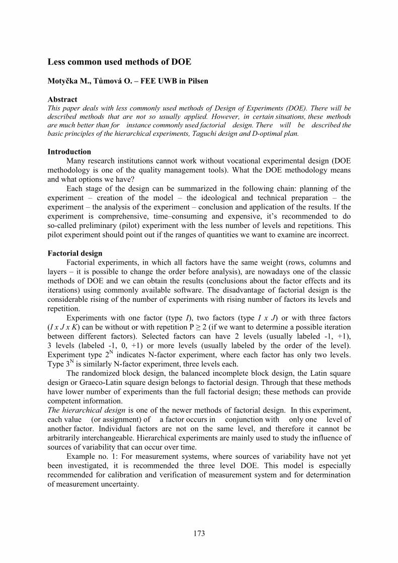
Less common used methods of DOE

Motyčka M., Tůmová O. – FEE UWB in Pilsen

Abstract This paper deals with less commonly used methods of Design of Experiments (DOE). There will be

described methods that are not so usually applied. However, in certain situations, these methods

are much better than for instance commonly used factorial design. There will be described the

basic principles of the hierarchical experiments, Taguchi design and D-optimal plan.

Introduction

Many research institutions cannot work without vocational experimental design (DOE

methodology is one of the quality management tools). What the DOE methodology means

and what options we have?

Each stage of the design can be summarized in the following chain: planning of the

experiment – creation of the model – the ideological and technical preparation – the

experiment – the analysis of the experiment – conclusion and application of the results. If the

experiment is comprehensive, time–consuming and expensive, it’s recommended to do

so-called preliminary (pilot) experiment with the less number of levels and repetitions. This

pilot experiment should point out if the ranges of quantities we want to examine are incorrect.

Factorial design

Factorial experiments, in which all factors have the same weight (rows, columns and

layers – it is possible to change the order before analysis), are nowadays one of the classic

methods of DOE and we can obtain the results (conclusions about the factor effects and its

iterations) using commonly available software. The disadvantage of factorial design is the

considerable rising of the number of experiments with rising number of factors its levels and

repetition.

Experiments with one factor (type I), two factors (type I x J) or with three factors

(I x J x K) can be without or with repetition P ≥ 2 (if we want to determine a possible iteration

between different factors). Selected factors can have 2 levels (usually labeled -1, +1),

3 levels (labeled -1, 0, +1) or more levels (usually labeled by the order of the level).

Experiment type 2N indicates N-factor experiment, where each factor has only two levels.

Type 3N is similarly N-factor experiment, three levels each.

The randomized block design, the balanced incomplete block design, the Latin square

design or Graeco-Latin square design belongs to factorial design. Through that these methods

have lower number of experiments than the full factorial design; these methods can provide

competent information.

The hierarchical design is one of the newer methods of factorial design. In this experiment,

each value (or assignment) of a factor occurs in conjunction with only one level of

another factor. Individual factors are not on the same level, and therefore it cannot be

arbitrarily interchangeable. Hierarchical experiments are mainly used to study the influence of

sources of variability that can occur over time.

Example no. 1: For measurement systems, where sources of variability have not yet

been investigated, it is recommended the three level DOE. This model is especially

recommended for calibration and verification of measurement system and for determination

of measurement uncertainty.

173

1st level – is the lowest level. The measurements are done in the short time

period (during one day, or one shift) and it is observed in particular to

repeatability of measurements. It includes J repeated measurements.

2nd

level – The measurement are done during few days (or similar time period),

and it includes the time period of K days (or similar).

3rd

level – is the highest level. The iterations are separated by the months. It is

includes L – iterations during this time period.

The measurement response model for hierarchical experiment is:

, (1)

where µ is the true value, γl is the effect of lth

iteration, δl,k is the effect of different days, e is

a random error effect (jth

repetition in the kth

day, when the measurement is repeated for the

lth

iteration).

Table 1: ANOVA for hierarchical experiment

Source of

variability

Sum of

Squares SS

Degrees of freedom

DF

Mean Square MS Expected Mean

Square

Iterations SSR L – 1 MSR 22

DJ +JK

2

R

Day (iterations) SSD (R) L (K – 1) MSD (R) 22

DJ

Error SSE LK (J - 1) MSE 2

Total SST - -

Where the variance of random error is , is the variance of days and is the variance of

iterations.

If we compare the ANOVA table in the standard factorial experiments with table no. 1,

we find out differences in the determination of degrees of freedom and in the related mean

square calculations. The expected values of variations for individual effects (factors) will be

also different. It is obvious that in hierarchical experiments we cannot arbitrary order

individual levels, because the results will not be correct.

Taguchi approach of DOE

How it was noted above, in the full factorial design is necessary to carry out the large

number of experiments. It’s obvious, that it isn’t acceptable in the common usage. The main

idea of the Taguchi approach is the reduction of number of experiments. So called

Orthogonal Arrays are used for this purpose. These arrays define the setting of particular

factors for each experiment. These orthogonal arrays are the basic knowledge of Taguchi

approach of DOE.

Fig. 1: The hierarchical design balanced and unbalanced

3th

level

2nd

level

1st level

174

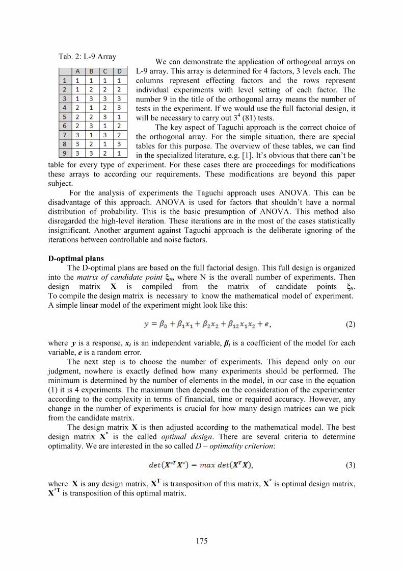
We can demonstrate the application of orthogonal arrays on

L-9 array. This array is determined for 4 factors, 3 levels each. The

columns represent effecting factors and the rows represent

individual experiments with level setting of each factor. The

number 9 in the title of the orthogonal array means the number of

tests in the experiment. If we would use the full factorial design, it

will be necessary to carry out 34 (81) tests.

The key aspect of Taguchi approach is the correct choice of

the orthogonal array. For the simple situation, there are special

tables for this purpose. The overview of these tables, we can find

in the specialized literature, e.g. [1]. It’s obvious that there can’t be

table for every type of experiment. For these cases there are proceedings for modifications

these arrays to according our requirements. These modifications are beyond this paper

subject.

For the analysis of experiments the Taguchi approach uses ANOVA. This can be

disadvantage of this approach. ANOVA is used for factors that shouldn’t have a normal

distribution of probability. This is the basic presumption of ANOVA. This method also

disregarded the high-level iteration. These iterations are in the most of the cases statistically

insignificant. Another argument against Taguchi approach is the deliberate ignoring of the

iterations between controllable and noise factors.

D-optimal plans

The D-optimal plans are based on the full factorial design. This full design is organized

into the matrix of candidate point ξN, where N is the overall number of experiments. Then

design matrix X is compiled from the matrix of candidate points ξN.

To compile the design matrix is necessary to know the mathematical model of experiment.

A simple linear model of the experiment might look like this:

, (2)

where y is a response, xi is an independent variable, βi is a coefficient of the model for each

variable, e is a random error.

The next step is to choose the number of experiments. This depend only on our

judgment, nowhere is exactly defined how many experiments should be performed. The

minimum is determined by the number of elements in the model, in our case in the equation

(1) it is 4 experiments. The maximum then depends on the consideration of the experimenter

according to the complexity in terms of financial, time or required accuracy. However, any

change in the number of experiments is crucial for how many design matrices can we pick

from the candidate matrix.

The design matrix X is then adjusted according to the mathematical model. The best

design matrix X* is the called optimal design. There are several criteria to determine

optimality. We are interested in the so called D – optimality criterion:

, (3)

where X is any design matrix, XT is transposition of this matrix, X

* is optimal design matrix,

X*T

is transposition of this optimal matrix.

Tab. 2: L-9 Array

175

The product of is called the information matrix. The experiment design is called

D-optimal, if the determinant of information matrix is maximal. Computational complexity of

this analytic method is very large. E.g. for 3 factors, 3 levels each and 10 tests it is

c. 8.5 million combinations of design matrix. From that reason different numerical methods

are used.

Conclusions

The paper deals with specific methods of DOE. In the conclusion will follow a short

comparison of these methods.

The hierarchical experiments do not reduce the number of attempts, but their advantage

lies in the fact that they respect the distribution of factors level in the experiment. Factors at

lower levels are a part of the factor at higher level and thus it can be freely interchange.

The Taguchi approach is a standardized methodology. For a given type of experiment is

precisely defined the setting of each factor in each test. This is the main advantage of this

method.

D-optimal plans are one of the newer methodologies. This method is included in the

standard VDA 5. The main advantage of this method is the choice of the number of tests in

the experiment at our discretion. On the other hand this is a considerable disadvantage. To

low number of test may invalidate the experiment. When the number of test is too high, the

experiment can be economically unacceptable. In order to properly design this type

of experiment, it is necessary to have considerable knowledge about the analyzed process.

Acknowledgements

This research was funded by the Ministry of Education, Youth and Sports of the Czech

Republic, MSM 4977751310 – Diagnostics of Interactive Processes in Electrical Engineering.

The authors are grateful for the support of this program.

References

1. ROY, Ranjit K. Design of Experiments Using The Taguchi Approach. Toronto: Jonh

Wiley and Sons, 2001. 538 s. ISBN 0-471-36101-1.

2. MONTGOMERY, Douglas C. Design of Experiments. [s.l.]: Jonh Wiley and Sons, 2009.

656 s. ISBN 978-0-470-39882-1.

3. DE AGUIAR, P. F., et al. D-optimal designs. Chemometrics and Intelligent Laboratory

Systems . 1995, vol. 30, Issue 2, s. 199-210. Dostupný také z WWW:

http://www.sciencedirect.com.

4. ANDĚL, J.: Matematická statistika, Praha: SNTL/ALFA, 1978.

5. LIKEŠ, J.: Navrhování průmyslových experimentů, Praha: SNTL, 1968.

6. TŮMOVÁ, O.: Navrhování experimentů a jejich vyhodnocování v praxi; habilitační

práce, Plzeň: ZČU, 1996.

7. TŮMOVÁ O., TOMKOVÁ Z.: Návrhy experimentů pro diagnostikování interaktivních

dějů, dílčí VZ pro MSM, Plzeň: 2006.

8. ČSN P ISO/TS 21749: Nejistoty měření v metrologických aplikacích - opakovaná

měření a hierarchické experimenty.

Authors

Ing. Martin Motyčka, Doc. Ing. Olga Tůmová, CSc.: Department of Technologies and Measurement,

Faculty of electrical Engineering, University of West Bohemia in Pilsen; Univerzitní 8, 306 14 Pilsen;

e-mail: [email protected], [email protected].

176

Analysis of induction machine reliability by means of FRA method Poliak, J., Gutten, M. – FEE UŽ Žilina Abstract This article deals with a description of methods of an experimental analysis - SFRA method concern-ing the actual reliability of windings and magnetic circuit of the induction machine. Introduction

Reliability of a technical device cannot be set with an absolute certainty. Reliability can be considered as a quality time fragment which is affected by technological discipline and a level of personnel qualification.

In all applications we can see that decreasing level of reliability comes with: • higher levels of sophistication of an equipment, • harsh work environment.

In current practise of prophylactics of power transformers dominate methods evaluating

dielectric-electric parameters focused on insulation system or on induction machine winding. From a theoretical analysis a probability of faultless operation can be defined by means

of fault intensity as follows:

( )( )∫−

=

t

dtt

etR 0

λ

(1) where: λ – fault intensity, t – time in operation. In a period of random faults of a system, if assumed that λ is constant, formula (1) can

be simplified to

( ) tetR λ= (2) Presumption stemming from formulas (1) and (2) has a rational basis. Value λ is af-

fected by physical, mechanical, chemical and technological factors, under which influence λ can exponentially change. To solve this problem it is particularly suitable to apply analysis of current passing through windings which cause losses.

Induction motors are a critical component of many industrial processes and are fre-

quently integrated in commercially available equipment and industrial processes. The studies of induction motor behaviour during abnormal conditions and the possibil-

ity to diagnose these conditions have been a challenging topic for many electrical machine researchers. The major faults of electrical machines can broadly be classified as the following [2], [3]:

• stator faults resulting in the opening or shorting of one or more of a stator phase wind-ings,

• abnormal connection of the stator windings, • broken rotor bar or cracked rotor endings, • static and/or dynamic air-gap irregularities, • bent shaft (akin to dynamic eccentricity) which can result in a rub between the rotor

and stator, causing serious damage to stator core and windings. In recent years, intensive research [3], [4] effort has been focused on the technique of

monitoring and diagnosis of electrical machines and can be summarized as follows:

177

• time and frequency domain analysis (e.g. FRA method), • time domain analysis of the electromagnetic torque and flux phasor, • temperature measurement, infrared recognition, radio frequency (RF) emission moni-

toring, • motor current signature analysis (MCSA), • detection by space vector angular fluctuation (SVAF), • noise and vibration monitoring, • acoustic noise measurements, • harmonic analysis of motor torque and speed, • model, artificial intelligence and neural network based techniques.

Of all the above techniques, MCSA and FRA methods are the best possible option: it is

non-intrusive and uses the stator winding as the search coil; it is not affected by the type of load and other asymmetries.

Diagnostics of electric machines by FRA method

FRA method belongs to current most effective analyses and allows to detect the influ-ences of short-circuit currents, overcurrents and other effects damaging either winding or magnetic circuit of the electric machines. This all can be performed without a necessity of decomposition of device and subsequent winding damage determination, which is very time consuming. [5]

The method of the high-frequency analysis (Frequency Response Analyzer –FRA) is also one of the methods of undisassembling diagnostics of electric machines (above all for transformers). No intervention to the construction of tested device is demanded, the whole measurement is performed on detached device (not under the voltage).

Measuring principles The frequency response characteristics of windings can be obtained using either the im-

pulse frequency response analysis (IFRA) method in the time domain or the sweep frequency response analysis (SFRA) method in the frequency domain.

In principle the two methods give the same results if the same connection method is used. However a frequency domain measurement using a method which records the ratio of the input and output voltages over the frequency range by using a sequence of narrow band spot measurements has been found to be particularly suitable for obtaining measurements in an electrically noisy environment. Making a series of narrow band measurements increases the signal to noise ratio and the dynamic range available. Measuring only at the exciting fre-quency also prevents any non-linearity of the test object (not usually a problem at the small signal levels employed) from affecting measurements at different frequencies. The measure-ment using this technique is conveniently made using a network analyser or similar instru-ment. This produces a frequency-varying sinusoidal voltage signal, applied to one terminal of the test winding with the input voltage being measured by a separate cable at that terminal and the response to this input measured at another terminal. [6]

Behaviours of induction motor winding responses by SFRA method According to [7] SFRA method determines the machine responses in a time or fre-

quency area. The time response measurement provides curve determination of the time re-sponse to the specific voltage impulse applied to winding input connection. The frequency response measurement consists in determination of amplitude eventually phase response to

178

the harmonic voltage of variable frequency applied to winding input. While the time response is the record of time behaviour of voltage, frequency response is the amplitude response de-pendence on frequency.

The machine measurement requires a setting up of the frequency range from 10 Hz to 2 MHz (Fig.2), whereas there is necessary to follow the right measuring technique to prevent various inaccuracies and faults. Input parameter of measuring system is voltage with value 10 V and its output parameter is current response (0÷90 dB) to change impedance for respective default frequency.

The behaviour of induction motor winding response reflects e.g. electromagnetic cou-plings between the stator winding and frame, between the windings of particular phases or between turns themselves of particular windings.

If induction motor is disconnected from three-phase networks (measurement is exer-cised at disconnected machine), i.e. speed rotary magnetic fields and rotor are null, is not pos-sible to diagnose rotor winding by this one method.

The connection of induction motor with squirrel-cage it is can follow for fig.1. Single amplitude and phase responses of stator windings motor are displayed for fig.2.

Fig.1: Wiring scheme of system M5100 and measured stator winding

a) Amplitude responses b) Phase responses Fig.2: Frequency responses of induction motor by SFRA method

frame

M5100 system

W V

U

179

The application of analysis of phase attenuation depending on frequency (fig.2b) is suit-able for more complete evaluation of winding condition. This analysis enables to assess the processes of stator winding damages during the particular operation influences. Conclusion

A relation between the response and the winding condition is definite, otherwise it is complicated. It is impossible to expect the assessment of concrete damage of winding from differences in response behaviors. The measurement results lead us only to a statement of the fact that some change of winding condition really occurred. Such test results are very helpful to decide, whether it is unavoidable to open and revise the transformer or not.

Acknowledgements

This work was supported by the Grant Agency VEGA from the Ministry of Education of Slovak Republic under contract 1/0548/09. References 1. Gutten, M., Kučera, S., Kučera, M., Šebök, M.: Analysis of power transformers reliabili-

ty with regard to the influences of short-circuit currents effects and overcurrents, PRZEGLĄD ELEKTROTECHNICZNY, p.62-64, R. 85 NR 7/2009, Poland.

2. VAS, P. “Parameter Estimation, Condition Monitoring, and Diagnosis of Electrical Ma-chines”, Clarendon Press, Oxford, 1993.

3. Neelam Mehala, Ratna Dahiya: Motor Current Signature Analysis and its Applications in Induction Motor Fault Diagnosis, In: INTERNATIONAL JOURNAL OF SYSTEMS APPLICATIONS, ENGINEERING & DEVELOPMENT Volume 2, Issue 1, 2007.

4. Cardoso, A. J. M., Cruz, S. M. A., Carvalho, J. F. S., Saraiva, E. S. : Rotor Cage Fault Diagnosis in Induction Motors by Park’s Vector Approach, IEEE, IAS’95 Orlando Flori-da, Oct. 1995, pp. 642–646.

5. Gutten M., Brandt M., Polanský R., Prosr P.: High-frequency analysis of three-winding autotransformers 400/121/34 kV, ADVANCES in EEE, No.1-2, 7/2008, Žilina, Slovakia.

6. Jayasinghe J.A.S.B., Wang Z.D., Jarman P.N., Darwin A.W.: The Winding Movement in Power Transformers: A Comparison of FRA Measurement Connection Methods. IEEE Transactions on Dielectrics and Electrical Insulation Vol. 13, No. 6; 2006, Canada.

7. Kvasnička V., Procházka R., Velek J.: Verification of method frequency characteristics in control room of distribution system Czech Republic, In Diagnostika 05, Plzeň 2005, Czech Republic.

Authors doc. Ing. Ján Poliak, Ph.D., doc. Ing. Miroslav Gutten, Ph.D; Department of Measurement and Appli-cation, Faculty of Electrical Engineering, University of Žilina, Veľký Diel , 01026 Žilina;; e-mail: [email protected] , [email protected].

180

Relation of electro insulating fluids to the environment

Trnka P., Souček J., Svoboda M. – FEE UWB in Pilsen

Abstract The most used insulating liquid in electrical engineering is mineral based oil. Mineral oil has

undesirable effect on the human organism and the environment. Careless handling and transport may

results in environmental disaster. The oil pollution relates to water, air and soil. This paper is focused

on negative impact of oils on the environment. Mineral oils are poorly biodegradable. From these

considerations it is necessary to replace mineral oils in the future. Vegetable oils and synthetic

organic esters are described as an alternative to mineral oils. These oils biodegradate fast and fully.

The effects of these oils on the human organism are described in this paper.

Introduction

Consumption of oil in the world is enormous. It is about 80 million barrels per day.

There are many predictions of the exhaustion of oil reserves. This prediction is dealt

geophysicist M. King Hubbert of Shell Oil. Hubbert devised the theory of peak oil. Graph of

peak oil describes the production of oil in million barrels per 1 day. This graph is shown in

Fig. 1 [1, 2, 3].

Fig. 1: Hubbert Peak Oil [1]

Peak oil consumption in this graph occurs around year 2014. For 150 years is mined

about 1 trillion barrels of oil and 1 trillion barrels is likely left. Hubbert's theory suggests that

oil will be exhausted in about 100 years. This theory does not claim to be infallible. However,

it is necessary to look for alternatives to oil today [1, 2, 3].

Mineral oils

The basis for the production of mineral oil is crude petroleum. Oil is a flammable liquid

that is extracted from underground oil deposits. Mineral oils are mixtures of saturated and

unsaturated hydrocarbons. The quality of mineral oils is dependent on the quality of mined oil

[2, 4].

Each of hydrocarbons act on the human organism and the environment in different

ways. Careless handling and transport may cause leakage of oil, which can have effects on

the environment and human health.

181

Air pollution is caused by the refining, storage and manipulation with oil. These

processes are released into the atmosphere volatile hydrocarbon vapors. These vapors pollute

air and deplete the ozone layer of Earth [2, 3, 6].

Contamination of water is most often caused by accidents of oil rigs and tankers. Into

the water is spilled thousands tons of oil in case of oil disaster. Leaked oil has significant

consequences for the ecosystem. Oil floating on the water creates a film that defends supply

oxygen into the water. This has resulted in suffocation of animals living under water. Oil also

affects the protective film of sea birds.

Soil contamination is caused by incorrect handling or accidents of pipelines. From

cracked pipelines can get into surrounding soil up to a thousand tons of oil. Oil spill can be

sized to several square kilometers. Leaked oil disrupts air ratio in the soil. This oil also

contaminates groundwater. The oil creates a greasy film on the soil surface. This results in

lower intake of air and water into the soil. For this reason, plants and animals die [2, 3, 6].

Oil also has undesirable effects on the human organism. Saturated hydrocarbons are not

toxic, but in certain quantities can cause adverse effects to humans. These hydrocarbons have

mainly narcotic effects, which means that it is changing human behavior. Inhalation of vapors

can damage the respiratory tract. In the liquid state may be absorbed into human skin and

cause allergic reactions [2, 4].

Unsaturated hydrocarbons are significantly more toxic than saturated hydrocarbons. The

most damaging are aromatic hydrocarbons. These hydrocarbons are highly carcinogenic. The

aromatic hydrocarbons can also negatively affect the human liver, kidneys or heart.

Unsaturated hydrocarbons also produce toxic ground-level ozone [2, 4, 5].

Biodegradability of mineral oil is very low. Biodegradability means degradation by

microorganisms. Microorganisms which are separated from oil deposits could be used for oil

decomposing process. The reaction of oil with microorganisms depends on the presence of

oxygen. Biodegradability is undesirable in storage. Microorganisms react with oil and while

producing organic acids. These acids can cause oxidative processes. Biodegradability of

hydrocarbons is described in the Tab. 1 [4].

Tab. 1: Biodegradability of hydrocarbons [4]

Hydrocarbon type Biodegradability

Alcans, izoalcans Very easily

degradable

Cycloalcanes with 1, 2, 5 and 6 cycles,

Arenes with 1 core Easily degradable

Cycloalcanes with 3 a 4 cycles,

Arenes with 2 and 3 cores

Medium easily

degradable

Arenes with 4 cores Resistant

Arenes with 5 or more cores Very strongly resistant

Vegetable oils and synthetic organic esters

As an alternative to mineral oil is now used vegetable oil as well. Vegetable oils consist

of mixtures of glycerol, esters, unsaturated and saturated fatty acids. These oils are extracted

from oleaginous plants. The seeds are pressed to obtain vegetable oil. This pressing is

performed by cold or hot pressing process. Pressed oil is refined to remove unwanted

substances. Refining can be done by neutralization, distillation and esterification [2].

182

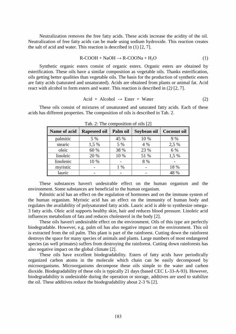
Neutralization removes the free fatty acids. These acids increase the acidity of the oil.

Neutralization of free fatty acids can be made using sodium hydroxide. This reaction creates

the salt of acid and water. This reaction is described in (1) [2, 7].

R-COOH + NaOH → R-COONa + H2O (1)

Synthetic organic esters consist of organic esters. Organic esters are obtained by

esterification. These oils have a similar composition as vegetable oils. Thanks esterification,

oils getting better qualities than vegetable oils. The basis for the production of synthetic esters

are fatty acids (saturated and unsaturated). Acids are obtained from plants or animal fat. Acid

react with alcohol to form esters and water. This reaction is described in (2) [2, 7].

Acid + Alcohol → Ester + Water (2)

These oils consist of mixtures of unsaturated and saturated fatty acids. Each of these

acids has different properties. The composition of oils is described in Tab. 2.

Tab. 2: The composition of oils [2]

Name of acid Rapeseed oil Palm oil Soybean oil Coconut oil

palmitic 5 % 45 % 10 % 9 %

stearic 1,5 % 5 % 4 % 2,5 %

oleic 60 % 38 % 23 % 6 %

linoleic 20 % 10 % 51 % 1,5 %

linolenic 10 % - 8 % -

myristic - 1 % - 18 %

lauric - - - 48 %

These substances haven't undesirable effect on the human organism and the

environment. Some substances are beneficial to the human organism.

Palmitic acid has an effect on the regulation of hormones and on the immune system of

the human organism. Myristic acid has an effect on the immunity of human body and

regulates the availability of polysaturated fatty acids. Lauric acid is able to synthesize omega-

3 fatty acids. Oleic acid supports healthy skin, hair and reduces blood pressure. Linoleic acid

influences metabolism of fats and reduces cholesterol in the body [2].

These oils haven't undesirable effect on the environment. Oils of this type are perfectly

biodegradable. However, e.g. palm oil has also negative impact on the environment. This oil

is extracted from the oil palm. This plant is part of the rainforest. Cutting down the rainforest

destroys the space for many species of animals and plants. Large numbers of most endangered

species (as well primates) suffers from destroying the rainforest. Cutting down rainforests has

also negative impact on the global climate [2].

These oils have excellent biodegradability. Esters of fatty acids have periodically

organized carbon atoms in the molecule which chain can be easily decomposed by

microorganisms. Microorganisms decompose these oils simple to the water and carbon

dioxide. Biodegradability of these oils is typically 21 days (based CEC L-33-A-93). However,

biodegradability is undesirable during the operation or storage, additives are used to stabilize

the oil. These additives reduce the biodegradability about 2-3 % [2].

183

Conclusions

Mineral oil has an undesirable effect on the environment and the human organism.

From this perspective it is appropriate to replace the petroleum based insulating oils.

Alternative solutions are vegetable oils and synthetic organic esters. These oils haven't such as

harmful effects on the environment and the human organism. Biodegradability of these oils is

approximately 21 days.

The price of vegetable oils is about 1.25 to 1.3 times the price of traditional mineral oils.

The disadvantage of these oils is higher acid value. This acidity has however no effects on the

paper in a transformer. Acidity also affects the oil life. It is necessary to focus research on

additives developing. The price of synthetic organic esters is about 4 to 8 times the price of

traditional mineral oils. This is a huge disadvantage. Therefore it is necessary to focus on

developing of new technologies of production of these oils.

Acknowledgement This study was carried out with the support of the NADACE ČEZ of the Czech

Electrical Energy Manufacturer and by project of the Ministry of Education, Youth and Sports

of Czech Republic, MSM 4977751310 – Diagnostic of Interactive Processes in Electrical

Engineering.

References

1. 2014: New and Improved Peak Oil Forecast. Miss Electric [online]. 16.3. 2010, [cit.

2011-07-11]. Available from WWW: <http://www.misselectric.com/?p=467>.

2. SOUČEK, Jakub. Refinement and regeneration process for electro-insulating fluids,

future horizons. Plzeň, 2011. pp. 12-56, [Diploma thesis], FEL ZČU, In Czech.

3. Peak oil. In Wikipedia : the free encyclopedia [online]. St. Petersburg (Florida) :

Wikipedia Foundation, 27. 9. 2005, last modified on 22. 2. 2011 [cit. 2011-04-01].

Available from WWW: <http://cs.wikipedia.org/wiki/Ropn%C3%BD_vrchol>, In Czech.

4. BLAŽEK, Josef; RÁBL, Vratislav. Basic principles of processing and using of

petroleum, VŠCHT Praha, 2006. pp.148-254, ISBN 80-7080-473-4, In Czech.

5. Aromatic hydrocarbons. Petroleum.cz [online]. 2007, n.1, [cit. 2011-03-05]. Available

from WWW: <http://www.petroleum.cz/ropa/aromaty.aspx>, In Czech.

6. MICHNÁČOVÁ, Žaneta. The occurrence and the importance of hydrocarbons in the

environment, Zlín, 2006.pp. 8-30, [Bachelor thesis], Tomas Bata University in Zlin, In

Czech.

7. Carboxylic acids. In Carboxylic acids - Wikipedie [online]. Praha : Wikipedie, 2011 [cit.

2011-01-23]. Available from WWW:

<http://cs.wikipedia.org/wiki/Karboxylov%C3%A9_kyseliny>, In Czech.

Authors doc. Ing. Pavel Trnka, Ph.D., Ing. Jakub Souček, Bc. Michal Svoboda; Department of technologies

and measurement, Faculty of Electrical Engineering, University of West Bohemia in Pilsen;

Univerzitní 8, 306 14 Plzeň; e-mail: [email protected], [email protected],

[email protected].

184

Is FMEA a risk? Tůmová O. – FEE UWB in Pilsen, Netolický P. – WiTTE Nejdek, spol. s r.o. Abstract This paper deals with the predictive method for reliability analysis - FMEA (Failure mode and effect analysis). Briefly describes the basic characteristics and different types of this method, its importance and customer requirements for this method. It is focused on the applications of this method. It evaluates the possible advantages and disadvantages in using. In regard to the practical use is carried out the consideration about possible recommendations for use in real applications. Introduction

FMEA is the shortcut for the Failure Mode and Effects Analysis (in Czech analýza způsobů a důsledků poruch, in German Fehler-Möglichkeits- und Einflussanalyse) and includes the team's analysis of possible failure modes of the design, evaluating their risks and the proposal and implementation of countermeasures for improving design quality [1]. This methodology is an instrument of quality and dependability planning. In the field of predictive analysis of the quality and dependability is used to detect failure mode before the real failure mode is present. This eliminates the high costs during the running period. Various information sources (for example [1], but other also) refer to the survey, that this tool can prevent up to 90% failures during the running period. For this reason, the FMEA methodology is often used and in some branches is its usage compulsory.

For the first time ever was FMEA methodology published in the United States of America in the military standard MIL-P-1629 in 1949 [2]. In the aviation industry was used in 1963 for Project Apollo [3]. After that the methodology started to spread into other sectors - 1975 Nuclear Industry, 1977 automotive industry (Ford). The methodology of risk analysis currently can be found in other areas - for example in medical technology, food industry (instrument known as HACCP system), construction equipment, software development. FMEA methodology is standardized in the general standard ČSN EN 60812:2007 Analysis techniques for system reliability - Procedure for Failure Mode and Effects Analysis (FMEA) [4].

In this area, there are standards specific for each branch of activity. The FMEA methodology is a compulsory part of the development of each product in the automotive industry (a compulsory part of the product development process according to methodology VDA4 or APQP). This methodology is standardized by two basic documents:

- FMEA reference manual for suppliers to companies Ford, Chrysler and GM (U.S. auto market) [5] and

- VDA Guide, Volume 4 – Ensures quality before mass production to suppliers in the German car manufacturers (Volkswagen, Audi, etc.) [3].

- In addition to these there are other standards for the process FMEA, which are no longer valid in general and relate to one customer. The examples include:

- Design Review Based on Failure Mode (DRBFM) from Toyota or - AMDEC - modified version used by the French car manufacturers, etc.

In addition, Ford has elaborated a general reference guide FMEA [5] in their follow-up manual [6] Basis of the methodology is always the same, differences are in some details, such as the system development sequence, procedure of analysis implementation, etc.

185

Types of FMEA’s All of the above mentioned publications differentiate two basic types of FMEA's:

1) design FMEA (KFMEA) and 2) process FMEA (PFMEA).

The main objective of KFMEA is failure analysis and component or system construction risks minimization. There are analyzed the different aspects / requirements for the design of component / equipment. The designer is responsible for this FMEA. Inputs to KFMEA are customer requirements, which are further developed, such as using QFD (Quality Function Deployment). Important inputs to KFMEA are the following information:

- object border (component / system), - analysis of relationships with others (the mechanical interface, the signal flow), - component / system failures.

For the component / system failures can be used another tools of dependability analysis, such as fault tree analysis (FTA) according to ČSN EN 61025:2007 [7].

The main objective of PFMEA is failure analysis and risk minimization in the process of component or equipment manufacturing. There are analyzed the different aspects / requirements for the production of component / system. The production engineer is responsible for this FMEA. Inputs to PFMEA are the following information:

- bill of material, - flowchart and - requirements for quality assurance of the process (e.g. from KFMEA or from customer

requirements). On the basis of the previous types of FMEA's can be defined other types, which differs

only in the subject of analysis. The types derived from KFMEA can include:

- FMEA concept - KFMEA of component / equipment for the concept of component / equipment (Simplified KFMEA), environmental FMEA - KFMEA component / equipment for the environmental aspects of design, FMEA for equipment - KFMEA for equipment and assembly parts and FMEA software - KFMEA focused on software development.

The types derived from PFMEA can include - FMEA concept - production process PFMEA for the concept of component / equipment (Simplified PFMEA), Service FMEA - PFMEA focused to service activities and Environmental FMEA - production process PFMEA focused on the environmental aspects.

FMEA can be used for unit production too. PFMEA can be used for manufacturing processes as well as for other business processes such as circulation of invoices, input checking process etc. The creation of FMEA procedure

The creation of FMEA can be described in four sequential steps: 1) Planning and preparation, 2) Risk Analysis, 3) Risk assessment and 4) Minimize the risk.

In the first step - the planning and preparation of FMEA - is carried out preparatory work prior to implementation of FMEA – a multidisciplinary team is established, the analyzed object is defined, gather information are collected, qualitative information from the history are evaluated, Fault tree analysis (FTA) is performed. The coordinator FMEA has the important

186

role. He is a member of the team, the team's moderator, provides formal (substantive) know-how.

The risk analysis is looking for potential failures, their consequences and causes. Then are mentioned the current prevention and detection measures. The exact sequence of activities in this step is dependent on customer specific requirements.

The numeric value is connected to the failure mode during risk assessment step. Each failure mode is evaluated by three parameters:

1) Severity of failure mode (S), 2) Occurrence of failure mode (O) and 3) Detection of failure mode (D).

Range for evaluation of each parameter is from 1 to 10. The higher is the number, the more severe is the parameter. Usually, the range of evaluation of each parameter is defined and it is dependent on customer specific requirements. The resulting risk RPN (risk priority number) is the product of individual parameters, ie. RPN = S. O. D.

In the last step - minimize the risk - is carried out an evaluation of the results and if necessary, countermeasures to minimize the risk are provided - to reduce the occurrence of failures or increase the detection of failures. Criteria for the identification of countermeasures can be (can be often used in combination):

- severity is high, f.e. S = 9, 10 (typically evalution is, that any legal requirement are not fullfilled),

- occurrence and / or detection is high, f.e. O ≥ 8 and / or D ≥ 8, - multiplication S . O is high (as criticality known) or - RPN number is high than 100 (disputed and debated criterium).

Risk Assessment in the implementation of FMEA

If you want to perform FMEA, it is appropriate to take into account some of the risks that are associated with the FMEA.

One of the risks is the failure or neglect of the first step FMEA process - planning and preparation. Not established or wrong established team is an important step that cannot be ignored. It must not be neglected role of FMEA coordinator. This man brings specific know-how to FMEA - such as work organization, a list of similar problems on other projects, a specialist in the methodology. FMEA coordinator is outside the risk analysis, moderates the discussion and gives additional (and sometimes “stupid”) questions to find the root cause of the potential issue.

Description and setting of range for evaluation severity, occurrence and detection is recommended activity in the steps of planning and preparation. Range of evaluation is often defined by the customer. There are also cases where it is possible to create a problem for the self-evaluation scale. This range of evaluation must have clearly defined criteria.

Next risk is the neglect of thorough preparation before the start of the FMEA. If it is not well defined object FMEA and its interface (component / equipment or process), addressing the issues arising primary purpose of analysis ("what exactly do you do?"). It is also desirable to have as much relevant historical data, because we prevent solutions to solved problems. Therefore, an FMEA is referred to as know-how of the company.

For this reason it is also worth considering how the FMEA data to processed and archived. If there is small number of FMEA analysis in the company, there is no need to address how to handle, such as MS Excel is sufficient. If there is a lot of FMEA analysis in the company, it is good to have some specialized software, with which it is then possible to

187

draw data across FMEA. It is also appropriate to define how the entry of certain items, which is useful during searching or document translation.

Do not forget the fact that the FMEA is a living document and that it should be taken into account all the current problems. Just then ensures that the FMEA database of knowledge and experience. Conclusion

To successfully and effectively avoid risks associated with reliability and quality of component / equipment or process, the FMEA is the appropriate tool. It is a useful tool that easily reveals the potential risks and uses the most important selection criteria. For those then suggest appropriate countermeasures to eliminate occurrence or to increase detection of the risk. To avoid the risks associated with the use - see previous text - is a good idea when FMEA is used. Then there is no formal document, but a tool, which can lead to significant cost reductions in the later stages of the project. References 1. PLURA, Jiří. Plánování a neustálé zlepšování jakosti. Praha : Computer Press, 2001. 244

s. ISBN 80-7226-543-1. 2. internet: http://de.wikipedia.org/wiki/FMEA, status 5.6.2011 3. VDA 4 - Zajišťování kvality před sériovou výrobou. Praha : Česká společnost pro jakost,

2007. 4. ČSN EN 60812. Techniky analýzy bezporuchovosti systémů - Postup analýzy způsobů a

důsledků poruch (FMEA). Praha : Český normalizační institut, 2007. 44 s. 5. DaimlerChrysler Corporation, Ford Motor Company, General Motors Corporation.

Analýza možných způsobů a důsledků poruch (FMEA). Praha : Česká společnost pro jakost, 2008. 143 s. ISBN 978-80-02-02101-8.

6. Ford Motor Company. FMEA Handbook Version 4.1. Dearborn: Ford Motor Company, 2004. 290 s.

7. ČSN EN 61025. Analýza stromu poruchových stavů (FTA). Praha : Český normalizační institut, 2007. 48 s.

Authors doc. Ing. Olga Tůmová, CSc.; Department of Technologies and Measurement, Faculty of Electrical Engineering, University of West Bohemia in Pilsen; Univerzitní 8, 306 14 Pilsen; e-mail: [email protected]. Ing. Petr Netolický, Ph.D.; WiTTE Nejdek, spol. s r.o., Rooseveltova 1299, 362 21 Nejdek; e-mail: [email protected].

188

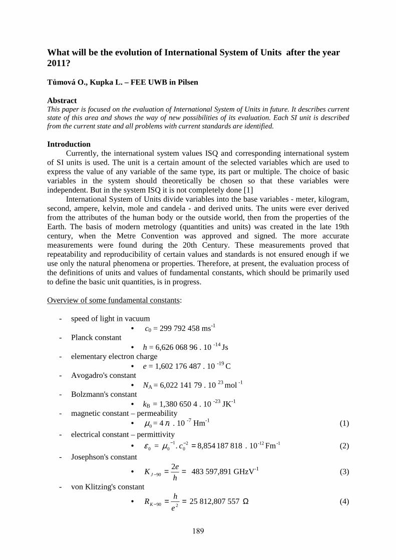
What will be the evolution of International System of Units after the year 2011? Tůmová O., Kupka L. – FEE UWB in Pilsen Abstract This paper is focused on the evaluation of International System of Units in future. It describes current state of this area and shows the way of new possibilities of its evaluation. Each SI unit is described from the current state and all problems with current standards are identified. Introduction

Currently, the international system values ISQ and corresponding international system of SI units is used. The unit is a certain amount of the selected variables which are used to express the value of any variable of the same type, its part or multiple. The choice of basic variables in the system should theoretically be chosen so that these variables were independent. But in the system ISQ it is not completely done [1]

International System of Units divide variables into the base variables - meter, kilogram, second, ampere, kelvin, mole and candela - and derived units. The units were ever derived from the attributes of the human body or the outside world, then from the properties of the Earth. The basis of modern metrology (quantities and units) was created in the late 19th century, when the Metre Convention was approved and signed. The more accurate measurements were found during the 20th Century. These measurements proved that repeatability and reproducibility of certain values and standards is not ensured enough if we use only the natural phenomena or properties. Therefore, at present, the evaluation process of the definitions of units and values of fundamental constants, which should be primarily used to define the basic unit quantities, is in progress. Overview of some fundamental constants:

- speed of light in vacuum • c0 = 299 792 458 ms-1

- Planck constant • h = 6,626 068 96 . 10 -14 Js

- elementary electron charge • e = 1,602 176 487 . 10 -19 C

- Avogadro's constant • NA = 6,022 141 79 . 10 23 mol -1

- Bolzmann's constant • kB = 1,380 650 4 . 10 -23 JK-1

- magnetic constant – permeability • 0µ = 4π . 10 -7 Hm-1 (1)

- electrical constant – permittivity

• 0ε = -1-1220

10 Fm10 . 8181878,854. =−− cµ (2)

- Josephson's constant

• ==− h

eK J

290 483 597,891 GHzV-1

(3)

- von Klitzing's constant

• ==− 290e

hRK 25 812,807 557 Ω (4)

189

The current definitions of base variables The length

The definition of length unit is since 1983 related to the speed of light c0 which is one of the fundamental constants. If in the future, precise measurements will show that the current standard of speed of light has not the constant value, there would be a standard adjusted to follow the speed of light. [1] The weight

The definition of weight unit depends on the value of international Pt-Ir standard which is stored in the International Institute in Sèvres near Paris. Even with the careful operation of storage, this standard is not quite stable and during its comparison with its copy there is some deviation, because while the international standard is becoming a little lighter, a copy of the 6 pieces, on the contrary is slightly heavier. Statistical methods can not be applied for definition the unit of weight, which should guarantee the sufficient repeatability and reproducibility. Currently, there is the redefinition of the kilogram prepared. They are now two international scientific researches proceeded to prepare the redefinition of this unit. The search for more optimal definition of the kilogram is continuing, either using the Avogadro's constant or Planck's constant. [3] The time

The current standard, the cesium clock as the time standard has the high stability and accuracy 10-15s. This is the reason that the current time unit "second" is likely to remain, and its definition derived from the operation of the cesium clock will not change. [1] The electric current

The current definition of the electric current is using magnetic effects of electric current, and therefore this unit is dependent on the weight unit. For the interaction of 3 constants, this equation is valid: 12

000 =cεµ , (5)

where 0µ = vacuum permeability,

c0 = constant speed of light in vacuum, 0ε = permittivity of vacuum.

Because of the weight unit redefinition is in process, on which is the unit of electric

current also depended, the professional discussion is currently in process whether to keep the electric current definition based on magnetic force effects (and keep a constant 0µ and 0ε ) or

define the electric current as the amount of charge transferred per time unit. Previously, the author of this article mentioned the metrological triangle for measuring

electric variables. In foreign research laboratories, the standard of electric current is prepared on the principle of the use of additional fundamental constant of the elementary electric charge of electrons - so-called electron turnstile.

The triangle of electrical quantities (Fig.1) represents two views. Macroscopic view expresses the correlation of electrical parameters (voltage, current and resistance) by Ohm's law, from the two known variables you can determine the third one. On the contrary, the microscopic view now shows three independent quantum phenomena that lead to three

190

different constants. This involves the possibility of creating a new standard of electric current. [2]

Fig. 1: The triangle of electrical quantities [2]

fe

hnfKnU J .

2... 1

90 == −− (6)

Ie

hIiRiIRU K 290 ).(. === − (7)

efI .= (8) The temperature

The kelvin unit will be redefined as well. The reason is that the temperature of the triple point of chemically pure water is not constant but depends slightly on the isotopic composition of water. Therefore, for the new definition will be used Boltzmann's constant kB and the relationship between temperature and energy will be used.

TkE B= , (9) where kB Bolzmann's constant T temperature in degrees Kelvin Amount of substance

The mole unit will be also redefined, the Avogadro's constant NA to be used, and thereby it will eliminate its dependence on the weight. [1] Brightness

The candela unit will not be redefined. [1] Conclusion

There is a tendency that all new definitions of the units were set that way to minimize the change of original basic unit, while repeatability and reproducibility would maintain the best possible parameters. This corresponds to the long-term trends, for example: the definition of the meter or the development of a second.

At the General Conference of Weights and Measures in this year there will be the discussion of redefinition of the kilogram, ampere, Kelvin and mole. Czech Republic is an

191

important part in all these activities – the 46th CIML meeting will be held on 10 – 14 October, 2011 in Prague. [4] Acknowledgements

This research was funded by the Ministry of Education, Youth and Sports of the Czech Republic, MSM 4977751310 – Diagnostics of Interactive Processes in Electrical Engineering. The authors are grateful for the support of this program. References: 1. Journal Metrologie 2/2010, edition 18, publisher ÚNMZ and ČMI, Czech Republic. 2. Journal Metrologie 2/2005, edition 14, publisher ÚNMZ and ČMI, Czech Republic. 3. Journal Metrologie annex 4/2010, edition 18, publisher ÚNMZ and ČMI, Czech

Republic. 4. Journal Metrologie 4/2010, edition 18, publisher ÚNMZ and ČMI, Czech Republic. Authors Doc. Ing. Olga Tůmová, CSc., Ing. Lukáš Kupka, Ph.D; Department of Technologies and Measurement, Faculty of electrical Engineering, University of West Bohemia in Pilsen; Univerzitní 8, 306 14 Pilsen; e-mail: [email protected], [email protected].

192

Estimation of Weibull Distribution Parameters for Reliability Žák P., Tučan M., Kudláček I. – FEE CTU in Prague Abstract The Weibull distribution is commonly used as a lifetime distribution in reliability test. The Weibull distribution is so often used because of its high variability - Weibull distribution can represent a decreasing, constant or increasing failure rate. Between the most commonly used methods we can include: least squares and maximum likelihood. In this paper we present the results of experiments aim at assessment of accuracy of these statistical estimation methods. In two-step test we used test data sets containing generated random values and data containing measured values of electrical resistance of electrically conductive adhesives. During the experiments we found that graphical method - Weibull plot and Weibull hazard plot - are relatively easily constructible and sometimes more accurate than the maximum likelihood method. Weibull plot and Weibull hazard plot give better results especially when datasets with censored data are analyzed. Weibull Analysis

The Weibull distribution is often used as a lifetime distribution in reliability. The Weibull distribution is so frequently used because of its variability - two-parameter Weibull distribution can represent all the three parts of the so-called bathtub curve. In this paper, we compare methods for estimating the parameters of Weibull distribution. We tested two basic methods: least squares and maximum likelihood. In two-step test we used test data sets containing generated random values and data containing measured values of electrical resistance of electrically conductive adhesives (ECA). Weibull Distribution

Weibull distribution is very flexible life distribution model often used in reliability. This distribution can be found with two or three parameters. The probability density function of a two-parameter Weibull random variable t is:

( )

1

( )tt

f t eβ

η

βββ ηη η

−− , , =

(1)

Where 0β > is the shape parameter, 0η > is the scale parameter (in reliability also called Weibull characteristic life) and t is in reliability most often time to failure, cycles to failures etc. The shape parameter is in reliability so important because it indicates the rate of change of the instantaneous failure rate with time. Characteristic life, η , is the time at which 63,2 % of the tested items are expected to fail.

Data types

When the times to failure of each item are exactly observed, the data are said to be complete. When analyzing life data, it is often necessary to include data of those items that have not already failed (censored data), or have not already failed by a failure mode we analyzing (suspended data) as well. Censored data can be divided into these two groups [1]:

• Right censored data – data sets that contain units that have not already failed by the end of the test.

• Interval censored data. This type of data frequently comes from reliability tests where the objects of interest are not continuously monitored.

193

• Left censored data. In left censored data, a time-to-failure is only known to be before a certain point of interest. When censored or suspended data are present, parameter estimation is more

complicated because standard techniques are not able to deal with these data.

Parameter Estimation Weibull parameter estimation can be done using graphical method via probability

plotting paper and hazard plotting, or analytically using maximum likelihood method. Graphical analysis consists of plotting the time-to-failure data on Weibull probability paper, fitting a line through these data, interpreting the plot and estimating the parameters using transformation of the Weibull equation into a linear form.

To make the Weibull plot we need to rank the time-to-failures data from the lowest to the highest. To calculate ranking position we use medium rank that can be generated in any spreadsheet program using the Beta inverse cumulative distribution function via: 1( 1)MR F p i N – i−= , , + (2)

where p is the confidence level, i is the rank order and N is the sample size. If it is not possible to calculate median ranks using the Beta distribution, we can use the Benard’s approximation.

Fig. 1: Example of the Weibull plot (time-to-

failures of two types of ECAs measured during a dump heat - low temperature cycles

test)

Fig. 2: Example of the Weibull hazard plot

(time-to-failures of two types of ECAs measured during a dump heat - low

temperature cycles test) This ranking defines the plotting positions for the time-to failures. Now the plot can be

constructed using three different methods: • Plotting directly to the Weibull probability paper - Weibull parameters are estimating

graphically from the plot. • Plotting Weibull probability plot using computer program - Weibull parameters are

estimating numerically using the method of least squares. Example of Weibull plot can be seeen in the figure 1. Weibull hazard plotting is also

good method for determining goodness-of-fit, but it can be also used for Weibull parameter estimation. The hazard plotting technique contains of ploting the estimated cumulative hazards against the time-to-failure on the Weibull hazard paper (ln-ln paper) (figure 2).

194

The maximum likelihood is the last used method. The principle of maximum likelihood parameter estimation (MLE) is to determine the parameters that maximize the probability (likelihood) of the sample data. Statistical background can be found in many publications for example in [2].

The goodness-of-fit

After all parameters are estimated, the goodness-of-fit is needed. If MLE technique is used, we can quantify uncertainty through confidence bounds. In the cases of graphical estimation methods we can use graphical method or numerical method. If time-to-failure data are distributed around a straight line in a probability plot or in a hazard plot, it is evidence that data are represented by the estimated distribution.

Design of experiment

To compare these three estimation techniques we used test data sets containing generated random values as well as data containing measured values of electrical resistance of electrically conductive adhesives. The first method has the advantage that we know the target value of Weibull parameters so we can assess the accuracy of the estimation technique. The second method is more realistic because it is possible to evaluate the variations of estimated parameters on the actual measured data from the reliability area of electrically conductive adhesives. Test data sets were generated using generator of random numbers from the Weibull distribution with specified parameters. When generating test data set we take into account three key parameters:

• Sample sizes. • Number of censored data. • Weibull shape parameter.

The first test data set thus consists of 27 combinations of tested parameters. To be the

test more reliable, always 10 sets of generated values with the combination of parameters was tested. 270 test files were tested in this part of experiment. The second test data set consists of two time-to failure data from reliability test made at our department. Both test files consist of 21 time-to-failures with censored data. For the purpose of this analysis a m-file in Matlab was programed. Conclusion

The results of the first part of experiment with randomly generated data sets are shown in table 1, where the most accurate method for each data set is reported and in parentheses is the percentage of its success. As we can see in table 1, for 0 % of censored observation and any combination of other parameters, the most accurate method is the MLE. However, for data files which contain censored data, MLE is not always the most accurate methodology. Especially for small data files containing censored observations, the Weibull hazard plot gives the best results. For larger data sets, the Weibull plot gives more accurate estimations. From the figure 3 we can see that Weibull plot tends to overestimate the shape parameter. The slope of the Weibull plot is often too steep.

195

Table 1: Table of the most accurate method in each tested group

Sample size (-) Censored data (%) Weibull parameter b (-) Most accurate methode

10

0 0.5 MLE (80 %) 1 MLE (60 %) 2 MLE (50 %)

10 0.5 Q-Q plot (80 %) 1 Hazard plot (70 %) 2 Hazard plot (60 %)

20 0.5 Q-Q plot (80 %) 1 Hazard plot (60 %) 2 Hazard plot (60 %)

20

0 0.5 MLE (60 %) 1 MLE (70 %) 2 MLE (80 %)

10 0.5 Q-Q plot (60 %) 1 MLE (70 %) 2 Hazard plot (40 %)

20 0.5 Q-Q plot (60 %) 1 MLE (70 %) 2 Q-Q plot (50 %)

40

0 0.5 MLE (60 %) 1 MLE (50 %) 2 MLE (60 %)

10 0.5 Q-Q plot (60 %) 1 MLE (50 %) 2 Hazard plot (50 %)

20 0.5 Q-Q plot (90 %) 1 MLE (40 %) 2 Hazard plot (50 %)

Fig. 3: Weibull shape parameter estimation accuracy of different estimation method shown on

real data sets

196

The general rules for choosing the most appropriate methodology can not be defined. When choosing a method of parameter estimation is necessary to take into account the particular nature of the analyzed data - in particular, the size of the test file, ratio of censored data and also the expected value of the Weibull shape parameter. Another aspect that influences the choice of methodology are the conditions under which we analyze the data. If the data analysis is performed with the aid of a computer, using all three methods at once does not pose a serious problem. On the other hand in case just a first outline is needed, as is often the case in the industry, simple graphical methods are preferable. Acknowledgements

This work was supported by the Grant Agency of the Czech Technical University in Prague, grant No. SGS10/163/OHK3/2T/13. References 1. IEC 60300-3-5. Dependability management: Application guide Reliability test conditions

and statistical test principles. 2001. 2. ARCHER, NORMAN P. A Computational Technique For Maximum Likelihood

Estimation With Weibull Models Reliability, IEEE Transactions on, vol.R-29, no.1, pp.57-62, April 1980.

3. IEC 61649. Weibull analysis. 2008.

Authors Ing. Pavel Žák, Ing. Marek Tučan, doc. Ing. Ivan Kudláček, CSc.; Department of Electrotechnology, Faculty of Electrical Engineering, Czech Technical University in Prague; Technicka 2, 16627 Prague 6; e-mail: [email protected], [email protected], [email protected].

197

Contribution to the study of lead-free technology in terms of LCA Žák P., Tučan M., Kudláček I. – FEE CTU in Prague Abstract The enormous expansion of lead-free soldering was initiated by the EU RoHS Directive 2002/95/EC. The purpose of this directive is to contribute to the protection of human health and the environmentally friendly recovery and disposal of waste electrical and electronic equipment. However, these changes brought also significant challenges into the electronics industry. Lead-free technologies often have to use more corrosive materials, or have less environmental stability. Another often encountered problem is higher temperature used in order to make reliable bonds. The aim of this paper is to describe advantages and disadvantages of technological shift to lead-free technology in terms of life cycle assessment and also from the point of view of reliability prediction and diagnostics. Motivation

Eutectic tin-lead (SnPb) solder has been during long time the primary choice for assembling electronics due to technological properties – especially low melting point. However, concern over lead’s and its toxicity have resultedinto restriction of its use – RoHS directive (2002/95/EC) in the EU and similar directives in other countries. Although the technological performance of lead-free has been studied, their life-cycle environmental impacts have not yet been evaluated in details.

In this paper first result of life cycle assessment (LCA) of model printed circuit board assembled using lead-free a SnPb solder are presented. We tried to compare both lead-based and lead-free solder alternatives and we focused this part of study on impacts on energy use, human toxicity, and ecological toxicity during the production phase.The results form LCAmethodologycanalso beusedtooptimizethe reliabilityof the finalproductas well asto finderrorsin the manufacturingprocess.

Life cycle assessment

LCA is often used to identifying possibilities to improve the environmental performance of certain product at various points in its life cycle. LCA is a methodology defined in ISO 14 040 standard that can be used for comprehensive analysis of the environmental consequences of a product system during its whole life. In this paper we present results of investigation focused on a product's life cycle from raw material acquisition to production (cradle-to-gate system). Complete LCA study is divided into four phases:

a) Goal and scope definition phase, b) Inventory analysis phase (LCI), c) Impact assessment phase (LCIA), and d) Interpretation phase. From this point of view we have done only LCI. For simulation we used professional

software for LCA called SimaPro. As a functional unit we defined a model case – 1 m2 of standard PCB.

The technology of Soldering

In this paper we evaluated the process of reflow soldering not the process of wave soldering. Soldering paste is in this mounting technology deposited on a printed circuits board

198

Fig. 1: Product system of SnPb soldering process.

Fig. 2: Product system of lead-free soldering proces.

(PCB) using stencil print. It is then processed using reflow soldering in a reflow oven with usually IR or hot air heating system.

The main difference between classic soldering and lead-free is higher temperature required for proper soldering of the latter. This difference usually ranges from 20°C to 30°C more and requires, among others, parts and fluxes adjusted to the new technology. Especially the fluxes have to be more aggressive and may contribute to corrosion of electronic devices.

For simulation we used life cycle inventory data in EcoInvent Database in version 2.1.

0,00422 m3 Building,

multi-storey/RER/ I U

38,1

21,4 MJ Electricity, high

voltage, production UCTE, 66,1

20,4 MJ Electricity,

medium voltage,

64,3

21,6 MJ Electricity,

production mix

66

1 m2 Mounting,

surface mount

114

2,08E-7 p Printed wiring board mounting

49,5

1 p Pb assembly

114

0,00423 m3

Building,

multi-storey /RER/I

U

38,2

27,2 MJ

E lectricity , high

v oltage,

production UC TE,

83,9

26 MJ

Electricity ,

medium v oltage,

production UC TE,

81,9

27,5 MJ

Electricity ,

production mix

UCTE/UC TE U

83,9

0,0807 kg

Solder, paste,

Sn95.5A g3.9C u0.

6, for electronics

38,9

1 m2

Mounting, surface

mount technology ,

Pb-free

138

2,08E-7 p

Printed w iring

board mounting

plant/GLO /I U

49,5

1 p

Pb-free

138

199

Life-Cycle Inventory Life-cycle inventory (LCI) includes identifying and quantifying all material and

resource inputs, and all emission and product outputs. Final product system of Sn/Pb soldering can be seen in the figure 1 and lead-free soldering in the figure 2. In order to make these uncluttered we used cut-off criteria at the level of 20 % i.e. these figures show only processes that consume more than 20 % of total energy. Both product systems are very similar the main difference between these product system is in their total energy consumption. Conclusion

Decision of the EU RoHS Directive 2002/95/EC, which has been valid since June 2006, appears to be somewhat premature and contradictory according to experience in the use of lead-free solders. Implementation of lead-free soldering technology brings a number of new demands, such as:

Higher energy requirements Change of parts Change of flux Change of materials for wave soldering machinery Change of cleaning technology

As seen above, the changes concern many aspects of the electronic production and often

bring in serious problems. The LCA method offers the opportunity to mitigate risks by helping the electronics industry to identify lead-free solders that are less toxic and less energy consuming.

Energy use impact scores are the sum of electrical and fuel energy inputs. For its calculation we used Cumulative Energy Demand LCA method defined in SimaPro software. Electricity use in the reflow application process is the main driver for this impact category. According to table 1 SAC solder has the highest impact score in these categories especially due to the energy used during silver extraction and processing. The second consuming part of mounting technology is a reflow process. Reflow process is due to higher melting temperature of SAC solder more power consuming in case of lead-free solders.

Tab. 1: Table of the most accurate method in each tested group.

Impact category Unit Pb-free SnPb Non renewable, fossil MJ-Equivalent 95.25 79.65

Non-renewable, nuclear MJ- Equivalent 33.06 26.20 Renewable, biomass MJ- Equivalent 5.04 4.76

Renewable, wind, solar, geothermal MJ- Equivalent 0.58 0.46 Renewable, water MJ- Equivalent 5.17 4.13

Sum MJ- Equivalent 139.10 115.19

The impact scores for the effects of global warming and climate change are calculated

using the mass of a greenhouse gases released to air, modified by a global warming potential equivalency factor. Global warming impacts follow the trend observed for the energy use category (i.e., SAC is driven by the upstream stage, SnPb and SnCu are driven by the use/application stage) due to the large amounts of electrical energy used over the life-cycle of these solders. Electricity generation produces considerable amounts of carbon dioxide, a

200

global warming gas. Unlike the paste solders where the global warming impacts are dominated by the use/application stage, both the upstream and use/application stages contribute significantly to the global warming impacts for each of the bar solders. This is because the reflow process uses more energy than the wave process and thus dominates the impacts for paste solder.

Fig. 3: Bar chart of impact on different impact categories.

Acknowledgements

This work was supported by the Grant Agency of the Czech Technical University in Prague, grant No. SGS10/163/OHK3/2T/13. References 1. ISO 14040. Environmental management – Life Cycle Assessment – Principles and

Framework. 2006. 2. Solders in Electronics: A Life-Cycle Assessment Summary. University of Tennessee.

2005. Authors Ing. Pavel Žák, Ing. Marek Tučan, doc. Ing. Ivan Kudláček, CSc.; Department of Electrotechnology, Faculty of Electrical Engineering, Czech Technical University in Prague; Technicka 2, 16627 Prague 6; e-mail: [email protected], [email protected], [email protected].

Comparing 1 p 'Pb-free' with 1 p 'Pb assembly'; Method: Eco-indicator 99 (H) V2.06 / Europe EI 99 H/H / weighting

Pb-free Pb assembly

Human Health Ecosystem Quality Resources

Pt

2,2

2,1

2

1,9

1,8

1,7

1,6

1,5

1,4

1,3

1,2

1,1

1

0,9

0,8

0,7

0,6

0,5

0,4

0,3

0,2

0,1

0

201

ISSN 1802-4564

Proceedings of the International Conference

Diagnostika `11held 6. - 8. September 2011 in Kašperské Hory

by DTM, FEE, UWB

Publisher: University of West Bohemia

All the papers were reviewed by conference advisory board. This publication was published using the manuscripts supplied by their authors. All mistakes in manuscripts there could be changed, nor could the English be checked completely. The readers are therefore asked to excuse any diferencies in this publication which may have arisen from the above causes.

Pilsen 2011

Editor: prof. Ing. Václav Mentlík, CSc.Cover design: Václav BočekName: Diagnostika `11Publisher: University of West BohemiaPrint: MK.Tisk, Plzeň, 2011ISBN 978-80-261-0020-1