University of Kentucky UKnowledge eses and Dissertations--Mechanical Engineering Mechanical Engineering 2017 DEVELOPMENT OF A SUPPLIER SEGMENTATION METHOD FOR INCREASED RESILIENCE AND ROBUSTNESS: A STUDY USING AGENT BASED MODELING AND SIMULATION Adam J. Brown University of Kentucky, [email protected] Author ORCID Identifier: hps://orcid.org/0000-0003-1184-2556 Digital Object Identifier: hps://doi.org/10.13023/ETD.2017.416 Click here to let us know how access to this document benefits you. is Doctoral Dissertation is brought to you for free and open access by the Mechanical Engineering at UKnowledge. It has been accepted for inclusion in eses and Dissertations--Mechanical Engineering by an authorized administrator of UKnowledge. For more information, please contact [email protected]. Recommended Citation Brown, Adam J., "DEVELOPMENT OF A SUPPLIER SEGMENTATION METHOD FOR INCREASED RESILIENCE AND ROBUSTNESS: A STUDY USING AGENT BASED MODELING AND SIMULATION" (2017). eses and Dissertations-- Mechanical Engineering. 100. hps://uknowledge.uky.edu/me_etds/100

Welcome message from author
This document is posted to help you gain knowledge. Please leave a comment to let me know what you think about it! Share it to your friends and learn new things together.
Transcript

University of KentuckyUKnowledge
Theses and Dissertations--Mechanical Engineering Mechanical Engineering
2017
DEVELOPMENT OF A SUPPLIERSEGMENTATION METHOD FORINCREASED RESILIENCE ANDROBUSTNESS: A STUDY USING AGENTBASED MODELING AND SIMULATIONAdam J. BrownUniversity of Kentucky, [email protected] ORCID Identifier:
https://orcid.org/0000-0003-1184-2556Digital Object Identifier: https://doi.org/10.13023/ETD.2017.416
Click here to let us know how access to this document benefits you.
This Doctoral Dissertation is brought to you for free and open access by the Mechanical Engineering at UKnowledge. It has been accepted for inclusionin Theses and Dissertations--Mechanical Engineering by an authorized administrator of UKnowledge. For more information, please [email protected].
Recommended CitationBrown, Adam J., "DEVELOPMENT OF A SUPPLIER SEGMENTATION METHOD FOR INCREASED RESILIENCE ANDROBUSTNESS: A STUDY USING AGENT BASED MODELING AND SIMULATION" (2017). Theses and Dissertations--Mechanical Engineering. 100.https://uknowledge.uky.edu/me_etds/100

STUDENT AGREEMENT:
I represent that my thesis or dissertation and abstract are my original work. Proper attribution has beengiven to all outside sources. I understand that I am solely responsible for obtaining any needed copyrightpermissions. I have obtained needed written permission statement(s) from the owner(s) of each third-party copyrighted matter to be included in my work, allowing electronic distribution (if such use is notpermitted by the fair use doctrine) which will be submitted to UKnowledge as Additional File.
I hereby grant to The University of Kentucky and its agents the irrevocable, non-exclusive, and royalty-free license to archive and make accessible my work in whole or in part in all forms of media, now orhereafter known. I agree that the document mentioned above may be made available immediately forworldwide access unless an embargo applies.
I retain all other ownership rights to the copyright of my work. I also retain the right to use in futureworks (such as articles or books) all or part of my work. I understand that I am free to register thecopyright to my work.
REVIEW, APPROVAL AND ACCEPTANCE
The document mentioned above has been reviewed and accepted by the student’s advisor, on behalf ofthe advisory committee, and by the Director of Graduate Studies (DGS), on behalf of the program; weverify that this is the final, approved version of the student’s thesis including all changes required by theadvisory committee. The undersigned agree to abide by the statements above.
Adam J. Brown, Student
Dr. Fazleena Badurdeen, Major Professor
Dr. Haluk Karaca, Director of Graduate Studies

DEVELOPMENT OF A SUPPLIER SEGMENTATION METHOD FOR INCREASED
RESILIENCE AND ROBUSTNESS: A STUDY USING AGENT BASED MODELING
AND SIMULATION
DISSERTATION
A dissertation submitted in partial fulfillment of the
requirements for the degree of Doctor of Philosophy in the
College of Engineering
at the University of Kentucky
By
Adam J. Brown
Lexington, Kentucky
Director: Dr. Fazleena Badurdeen, Professor of Mechanical Engineering
Lexington, Kentucky
2017
Copyright © Adam J. Brown 2017

ABSTRACT OF DISSERTATION
DEVELOPMENT OF A SUPPLIER SEGMENTATION METHOD FOR INCREASED
RESILIENCE AND ROBUSTNESS: A STUDY USING AGENT BASED MODELING
AND SIMULATION
Supply chain management is a complex process requiring the coordination of numerous
decisions in the attempt to balance often-conflicting objectives such as quality, cost, and
on-time delivery. To meet these and other objectives, a focal company must develop
organized systems for establishing and managing its supplier relationships. A reliable,
decision-support tool is needed for selecting the best procurement strategy for each
supplier, given knowledge of the existing sourcing environment. Supplier segmentation is
a well-established and resource-efficient tool used to identify procurement strategies for
groups of suppliers with similar characteristics. However, the existing methods of
segmentation generally select strategies that optimize performance during normal
operating conditions, and do not explicitly consider the effects of the chosen strategy on
the supply chain’s ability to respond to disruption. As a supply chain expands in complexity
and scale, its exposure to sources of major disruption like natural disasters, labor strikes,
and changing government regulations also increases. With increased exposure to
disruption, it becomes necessary for supply chains to build in resilience and robustness in
the attempt to guard against these types of events. This work argues that the potential
impacts of disruption should be considered during the establishment of day-to-day
procurement strategy, and not solely in the development of posterior action plans. In this
work, a case study of a laser printer supply chain is used as a context for studying the
effects of different supplier segmentation methods. The system is examined using agent-
based modeling and simulation with the objective of measuring disruption impact, given a
set of initial conditions. Through insights gained in examination of the results, this work
seeks to derive a set of improved rules for segmentation procedure whereby the best
strategy for resilience and robustness for any supplier can be identified given a set of the
observable supplier characteristics.
KEYWORDS: Resilience, Robustness, Supplier Relationship Management, Supplier
Segmentation, Agent-Based Modeling and Simulation

Adam J. Brown
August 18, 2017

DEVELOPMENT OF A SUPPLIER SEGMENTATION METHOD FOR INCREASED
RESILIENCE AND ROBUSTNESS: A STUDY USING AGENT BASED MODELING
AND SIMULATION
By
Adam J. Brown
Dr. Fazleena Badurdeen
Director of Dissertation
Dr. Haluk Karaca
Director of Graduate Studies
_______August 18, 2017_________

This dissertation is dedicated to the many friends, family, colleagues, and acquaintances
whose support has enabled me to complete this degree, especially my parents (Jennifer
and David), Isaac Lee, Joseph Amundson, Jeremy Leachman, Nicholas Callihan, and my
sister (Ellen).

iii
ACKNOWLEDGEMENTS
Thanks to my advisor, Dr. Fazleena Badurdeen for continuous support throughout the
research process, and for giving me the opportunity to work on a variety of interesting and
challenging projects. I also thank the members of my Ph.D. committee: Dr. I.S. Jawahir,
Dr. Larry Holloway, Dr. Mike Li, and Dr. Tom Goldsby for the time they have dedicated
for review of my work and for their invaluable advice provided. Thanks, finally, to
everyone at the Institute for Sustainable Manufacturing (ISM) for creating a supportive and
pleasant environment in which to work.

iv
TABLE OF CONTENTS
ACKNOWLEDGEMENTS ............................................................................................... iii
LIST OF TABLES ............................................................................................................. vi
LIST OF FIGURES .......................................................................................................... vii
1 Introduction and Motivation ........................................................................................ 1
1.1 Complexity of Supply Chain Management .......................................................... 1
1.2 Key Definitions .................................................................................................... 4
1.3 Research Gap........................................................................................................ 8
2 Literature Review ...................................................................................................... 11
2.1 Supplier Segmentation ....................................................................................... 12
2.1.1 Portfolio Methods ....................................................................................... 13
2.1.2 Partnership Model ....................................................................................... 17
2.1.3 Involvement Methods ................................................................................. 19
2.1.4 Units of Differentiation ............................................................................... 19
2.1.5 Limitations of Existing Segmentation Methods ......................................... 20
2.2 Management Strategies for Increased Resilience............................................... 24
2.2.1 Supply Chain Visibility and Data Analysis ................................................ 27
2.2.2 Collaboration and Supplier Development ................................................... 30
2.2.3 Training, Learning, and Business Continuity Planning .............................. 32
2.2.4 Redundancy and Inventory Management ................................................... 34
2.2.5 Flexibility, Velocity, and Agility ................................................................ 36
2.2.6 Network Structure ....................................................................................... 38
2.2.7 Power and Dependency............................................................................... 40
2.3 Incorporating Resilience-Enabling Factors in Segmentation ............................. 41
3 Methodology for Comparison of Segmentation Methods ......................................... 45
3.1 Phase I: Develop Revised Segmentation Method .............................................. 45
3.2 Phase II: Framework for Comparative Analysis ................................................ 48
3.3 Phase III: Application to Case Study ................................................................. 48
3.4 Phase IV: Analysis of Results ............................................................................ 49
4 Analysis and Selection of Modeling and Simulation Paradigm ................................ 52
4.1 Agent-Based Modeling and Simulation ............................................................. 54
4.2 Supply Chain Applications of ABMS ................................................................ 57

v
5 Case Study ................................................................................................................. 68
5.1 Laser Printer Bill of Materials ............................................................................ 68
5.2 Data Collection ................................................................................................... 70
5.3 Segmentation Results ......................................................................................... 76
6 Model Development and Specifications .................................................................... 79
6.1 ABMS Requirements Determination and Specification .................................... 79
6.2 Agent Class and Activity Diagrams ................................................................... 84
6.3 ABMS Platform.................................................................................................. 98
7 Results ....................................................................................................................... 99
7.1 Establishment of Normal Operating Levels ....................................................... 99
7.2 Disruption Response Analysis for Baseline and Revised Cases ...................... 105
7.2.1 Disruption at Cartridge Supplier ............................................................... 107
7.2.2 Disruption at Toner Supplier .................................................................... 115
7.2.3 Disruption at Power Supply Supplier ....................................................... 120
7.2.4 Disruption at PCBA Supplier.................................................................... 126
7.3 Effects of Demand Seasonality and Disruption Severity ................................. 132
7.4 Baseline vs. Revised Comparison for all Scenarios ......................................... 137
8 Discussion ................................................................................................................ 140
9 Summary and Future Work ..................................................................................... 145
Appendix ......................................................................................................................... 147
A Comparison of Segmentation Methods ................................................................... 147
B Resilience-Enabling Factors Literature Review Summary Tables .......................... 150
C Simulation Results Tables ....................................................................................... 165
D Simulation User Guide ............................................................................................ 185
D.1 Overview of Data Input Files ........................................................................... 185
D.2 Simulation Use-Case 1: Single run with no disruptions .................................. 190
D.3 Simulation Use-Case 2: Multi-replication run with a disruption ..................... 194
References ....................................................................................................................... 198
VITA ............................................................................................................................... 205

vi
LIST OF TABLES
Table 2.1: Relationship strategies for supplier segments, adapted from (Rijt and Santerna
2010) ................................................................................................................................. 15
Table 3.1: Assessment variables for complexity of supply market .................................. 46
Table 3.2: Assessment variables for importance of purchasing ....................................... 47
Table 3.3: Procurement strategies for each supplier segment ........................................... 48
Table 4.1: Modeling Paradigms ........................................................................................ 53
Table 5.1: Variable assessment for market complexity .................................................... 73
Table 5.2: Variable assessment for purchasing importance .............................................. 74
Table 5.3: Summary of segmentation results for each supplier ........................................ 77
Table 5.4: Strategic sourcing options for each supplier .................................................... 79
Table 6.1: GPA descriptions for the proposed case study ................................................ 81
Table 6.2: Factors and levels for case study ..................................................................... 83
Table 6.3: KPI for case study ............................................................................................ 84
Table 6.4: Primary simulation actions .............................................................................. 86
Table 7.1: Summary of disruption scenarios .................................................................. 106

vii
LIST OF FIGURES
Figure 1.1: Supply chain network, adapted from (Lambert 2006) ..................................... 2
Figure 1.2: Risk management framework (Oehmen and Rebentisch 2010) ....................... 5
Figure 1.3: Disruption response profile (Brown and Badurdeen, 2015)............................. 7
Figure 1.4: Percentage of respondents reporting in each range # of disruption occurrences
(Alcantara 2014) ................................................................................................................. 8
Figure 2.1: Theoretical framework ................................................................................... 12
Figure 2.2: Supplier segmentation matrix, adapted from (Kraljic 1983) .......................... 14
Figure 2.3: Positive, neutral, and negative inter-firm relationships, (Ritter 2000) ........... 22
Figure 2.4: Collaboration based on type of relationship interdependency, (Persson and
Hakansson 2007) ............................................................................................................... 23
Figure 2.5: Literature review search terms to identify management strategies for
increased resilience ........................................................................................................... 25
Figure 2.6: Frequently mentioned strategies and characteristics of resilience ................. 27
Figure 2.7: Integration of traditional segmentation variables and resilience-enabling
factors ................................................................................................................................ 42
Figure 3.1: Steps for assessing segmentation method ...................................................... 45
Figure 4.1: Supply chain agent interactions, (Fox, Chionglo et al. 1993) ........................ 57
Figure 4.2: Supply chain ABMS search terms.................................................................. 59
Figure 4.3: Focus areas within literature on ABMS supply chain applications ................ 64
Figure 5.1: Laser printer components (Oki Data Systems 2007)...................................... 68
Figure 5.2: Laser printer tiered bill of materials ............................................................... 69
Figure 5.3: Global operations for laser printer supply chain ............................................ 71
Figure 5.4: Spatial representation of laser printer supply chain ....................................... 72
Figure 5.5: Results of baseline segmentation method ...................................................... 76
Figure 5.6: Results of revised segmentation method ........................................................ 77
Figure 6.1: Analysis pathways, adapted from (de Santa Eulalia 2009) ............................ 80
Figure 6.2: Supply chain cube, adapted from (de Santa Eulalia 2009) ............................. 82
Figure 6.3: Agent class diagram ....................................................................................... 85
Figure 6.4: Activity diagram for disruption implementation ............................................ 87
Figure 6.5: Activity diagram for read-demand ................................................................. 89
Figure 6.6: Activity diagram for production (normal operation) ...................................... 90
Figure 6.7: Activity diagram for production with disruption (with dual supplier) ........... 92
Figure 6.8: Activity diagram for production with disruption (without dual supplier) ...... 93
Figure 6.9: Activity diagram for production, setting order allocation levels after
disruption recovery ........................................................................................................... 95
Figure 6.10: Activity diagram for delivery (truck picks up haul) ..................................... 96
Figure 6.11: Activity diagram for delivery (deliver haul to buyer) .................................. 97
Figure 7.1: Final assembly inventory at DCs (Baseline) ................................................ 100
Figure 7.2: Comparison of lower bounds for final assembly inventory at DCs ............. 101
Figure 7.3: Comparison of lower bound for photoconductor inventory at DCs ............. 102

viii
Figure 7.4: Comparison of lower bound for cartridge inventory at DCs ........................ 103
Figure 7.5: Comparison of upper bound for total supply chain cost .............................. 104
Figure 7.6: Comparison of holding cost at each node .................................................... 105
Figure 7.7: Partial SC map showing disruption at cartridge supplier location 1 (Baseline)
......................................................................................................................................... 107
Figure 7.8: Inventory response to disruption at cartridge supplier location 1 (Baseline) 109
Figure 7.9: Total SC cost (Baseline) ............................................................................... 111
Figure 7.10: Partial SC map showing disruption at cartridge supplier location 1 (Revised)
......................................................................................................................................... 112
Figure 7.11: Inventory response to disruption at cartridge supplier location 1 (Revised)
......................................................................................................................................... 113
Figure 7.12: Total supply chain cost (Revised) .............................................................. 114
Figure 7.13: Inventory response to disruption at toner supplier (Baseline) .................... 116
Figure 7.14: Total SC cost with disruption at toner supplier (Baseline) ........................ 117
Figure 7.15: Inventory response to disruption at toner supplier (Revised)..................... 119
Figure 7.16: Total SC cost with disruption at toner supplier (Revised) ......................... 120
Figure 7.17:Partial SC map showing disruption at power supply supplier (Baseline) ... 120
Figure 7.18: Inventory response to disruption at power supply supplier (Baseline) ...... 122
Figure 7.19: Total supply chain cost with disruption at power supply (Baseline) ......... 123
Figure 7.20: Partial SC map showing disruption at power supply supplier (Revised) ... 124
Figure 7.21: Inventory response to disruption at power supply supplier (Revised) ....... 125
Figure 7.22: Total SC cost with disruption at power supply supplier (Revised) ............ 126
Figure 7.23: Partial SC map showing disruption at PCBA supplier (Baseline) ............. 127
Figure 7.24: Inventory response to disruption at PCBA supplier (Baseline) ................. 128
Figure 7.25: Total SC cost with disruption at PCBA supplier (Baseline) ...................... 129
Figure 7.26: Inventory response to disruption at PCBA supplier (Revised) .................. 130
Figure 7.27: Total SC cost with disruption at PCBA supplier (Revised) ....................... 132
Figure 7.28: Seasonality and severity effects with disruption at cartridge supplier
(Baseline) ........................................................................................................................ 133
Figure 7.29: Seasonality and severity effects with disruption at cartridge supplier
(Revised) ......................................................................................................................... 133
Figure 7.30: Seasonality and severity effects with disruption at toner supplier (Baseline)
......................................................................................................................................... 134
Figure 7.31: Seasonality and severity effects with disruption at toner supplier (Revised)
......................................................................................................................................... 134
Figure 7.32: Seasonality and severity effects with disruption at power supply supplier
(Baseline) ........................................................................................................................ 135
Figure 7.33: Seasonality and severity effects with disruption at power supply supplier
(Revised) ......................................................................................................................... 136
Figure 7.34: Seasonality and severity effects with disruption at PCBA supplier (Baseline)
......................................................................................................................................... 136
Figure 7.35: Seasonality and severity effects with disruption at PCBA supplier (Revised)
......................................................................................................................................... 137

ix
Figure 7.36: Resilience & robustness to disruption at cartridge supplier ....................... 137
Figure 7.37:Resilience and robustness to disruption at toner supplier ........................... 138
Figure 7.38: Resilience and robustness to disruption at power supply supplier ............. 138
Figure 7.39: Resilience and robustness to disruption at PCBA supplier ........................ 139

1
1 Introduction and Motivation
1.1 Complexity of Supply Chain Management
In the text ‘Supply Chain Risk: A Handbook of Assessment, Management, and
Performance’, Zsidisin and Ritchie (2009) defined a supply chain as the “linkage of stages
in a process from the initial raw material or commodity sourcing through various stages of
manufacture, processing, storage, and transportation to the eventual delivery and
consumption by the end consumer” (ch.1). These linkages can exist between
geographically dispersed entities of the same organization, or between a company and its
external partners. Overall business capability is therefore a property of the supply chain
system and must be measured as a function of the performance of every partner in the
supply chain network (Fine 1999). Rather than existing as a series of linear connections
between buyers and suppliers, these systems are complex and competitive advantage must
be gained through the effective functioning of interconnected and overlapping networks
(Lambert 2006). A failure at any node or linkage in the supply chain network will have a
negative effect on the entire system.
Figure 1.1 represents a supply chain network and the different kinds of linkages that exist
between entities in the network.

2
Figure 1.1: Supply chain network, adapted from (Lambert 2006)
Supply chain managers at the focal company must make strategic decisions relating to not
only their immediate suppliers, but also their suppliers’ suppliers and so on leading back
to the procurement of raw materials. It should be determined which suppliers should be
actively managed, which ones should be kept at arm’s length but monitored regularly, and
which are best left to manage themselves. Then, for each managed connection in the
network, an appropriate procurement strategy should be specified and put into practice.
The procurement strategy defines the rules of buyer-supplier interaction such as when to
use dual sourcing, how much inventory should be kept on hand and where it should be
held, and how much visibility should be established and maintained. It is important to

3
predetermine for each connection what type of information the focal company is willing to
share with the suppliers and how frequently.
Decisions should be made on how and when to consider the potential effects of major
disruptions on supply chain performance. How does the choice of the day-to-day
procurement strategy affect the focal company’s ability to respond to disruption? If one of
the actively-managed first-tier suppliers fails due to an unexpected malfunction, it is
probable that management would become aware of the issue immediately and could
respond promptly. However, if the same failure occurs at a supplier that is not actively
managed, then there is a strong likelihood that the focal company’s response capability
would be less adept.
The questions relating to supply chain disruption management form the primary motivation
behind this research. A decision support tool is needed to help supply chain managers to
decide what type of relationships to develop with its supply base to best equip itself for
effective disruption response. At the same time, the decision support tool should consider
that an optimal strategy may not be attainable due to uncontrollable external factors, and
that suppliers will be making decisions to act in their own interest.
Supply chains can be described as socio-technical systems, meaning that they are
comprised of both a technical network of facilities linked by material and information flow
and a social network based on formal and informal exchanges of information (Behdani
2012). Supplier Relationship Management (SRM) is an established sub-process within the
realm of supply chain management that has the goal of providing structure and planning to
the development and maintenance of supplier relationships (Croxton, Garcia-Dastugue et
al. 2001). SRM creates the rules of interaction between buyer and supplier, including the
development of Product Service Agreements (PSA’s) or other contracts. The buyer-
supplier relationship can be as generic or as specialized as is necessary for the success and
satisfaction of both entities. The requirements for information exchange and coordination
increase rapidly as the complexity of the supply chain increases. Thus, it becomes
necessary to prioritize the management of critical suppliers. The identification of these
critical suppliers is one of the main outcomes of SRM and it is often achieved through a
process known as supplier segmentation. The segmentation process is used to determine

4
appropriate relationships for each supply chain member and can be an important step
toward ensuring the success of both the focal company and its partners. Different methods
of supplier segmentation are discussed further in Section 2.1.
Adding to the complexity of supply chain management is the fact that supply chain
networks must often be designed to meet conflicting objectives. As indicated by the “2010
and Beyond” research initiative which surveyed current and future issues pertinent to
supply chains, to be successful supply chains must compete on cost, responsiveness,
security, sustainability, resilience, and innovation (Melnyk, Davis et al. 2010). These
qualities represent only a subset of many other desirable supply chain characteristics. This
work will consider the performance trade-offs that exist between resilience against
disruptions and other objectives. The work explores the possibility of expanding the
application of supplier segmentation as a tool for increasing supply chain resilience and
robustness.
1.2 Key Definitions
Key terminology in risk management for the supply chain has been used with varying
consistency. It is important to state formally the foundational definitions as will be used
throughout the remainder of the work.
Risk management can be formally defined as “the identification, evaluation, and ranking
of the priority of risks followed by synchronized and cost-effective application of resources
to lessen, monitor, and control the probability and/or impact of unfortunate events” (ISO
2009). Figure 1.2 shows the framework established by ISO for risk management.

5
Figure 1.2: Risk management framework (Oehmen and Rebentisch 2010)
The ISO framework contains five core steps which occur sequentially, and two concurrent
steps which entail continuous monitoring and communication of the results (Oehmen and
Rebentisch 2010). The core steps begin with the establishment of context. This includes
selection of the product of interest and drawing of any boundaries for what will and will
not be considered. The center of the framework contains the three stages of risk assessment:
identification, analysis, and evaluation. Risk identification involves specification of any
events of interest which would have a negative impact on the supply chain performance.
The identification may attempt to uncover an exhaustive list of potential risk sources or
focus on a very specific scenario depending on the goals of the assessment. Next, risk
analysis is conducted to increase knowledge about the identified risk scenarios. This may
be done by establishing some ranking of likelihood of occurrence and significance of any
potential impact. Analysis is a data-intensive process and may rely on historical data or
domain expert opinions. Finally, risk evaluation is the stage in which results of analysis are

6
examined and the risks are prioritized. Risks needing immediate attention can be separated
from those needing continued monitoring and others which do not pose a significant threat.
Risk treatment follows the assessment stages and involves implementation of solutions to
reduce the threat level.
Risk can be succinctly defined as the ‘likelihood of conversion of a source of danger into
actual delivery of loss, injury, or some form of damage,’ (Garrick, 2008). The results of
risk identification and analysis can be specified by a set of risk triplets, where the items in
the triplet reflect the risk scenario, its estimated likelihood, and the consequence of its
occurrence (Abyaneh, Hassanzadeh et al. 2011).
𝑅 = {⟨𝑆𝑖, 𝑃𝑖, 𝑋𝑖⟩}, 𝑖 = 1,2, … 𝑁 Equation 1.1
Si represents a possible risk scenario, while Pi is the probability that the scenario will occur
and Xi is a measure of the consequence should the scenario occur. This approach is
especially geared towards high probability events, where the expected duration of the
problem can then be estimated based on past occurrences. This work emphasizes a kind of
risk scenario known as a disruption, defined as ‘an unintended and anomalous event
resulting in an exceptional situation that significantly threatens the course of normal
business operations’ (Wagner and Bode, 2009). Disruptions occur infrequently and it may
not be feasible to characterize them by their likelihood of occurrence. The consequence, or
severity, of a disruption is high. Low likelihood, high impact disruptions represent the
events for which an organization does not have experience upon which it can rely. Rather
than focusing on likelihood, organizations must focus on the recovery period and acting to
provide as many options for recovery as possible (Sheffi 2009).
Resilience is an important concept which refers to the ability of a system to recover from
a disruption. Resilience has been defined as the ‘ability of a system to return to its original
state or move to a new, more desirable state after being disturbed’ (Christopher and Peck
2004). Furthermore, it is important to distinguish the property of robustness which is
defined as ‘a measure of supply chain strength or an ability to remain effective under all

7
possible future scenarios’ (Klibi, Martel et al. 2010). The concepts of resilience and
robustness can be visually represented on a disruption response profile, such as the one
presented in Figure 1.3.
Figure 1.3: Disruption response profile (Brown and Badurdeen, 2015)
In Figure 1.3 the initial normal operating performance range for inventory can be seen
represented by the horizontal dashed lines. The inventory serves as a performance measure
on the y-axis and could be replaced by profitability, market share, production volume, or
perhaps some aggregate score based on many variables. The spread around the normal
performance level indicates the possible performance fluctuation due to operational
disturbances like machine downtime or demand fluctuations. In contrast, the performance
level drops well below the normal range when a disruption occurs. Robustness of the
supply chain is a representation of its ability to minimize performance degradation after a
disruption. The distance from normal operating performance to the minimum performance
level is a measure of robustness. Resilience, on the other hand, is measured along the time
axis. A more resilient supply chain will return to and remain in the normal operating range

8
more quickly after the disruption has ended. In general, the inventory level of more resilient
supply chain would spend less time below the normal operating range.
1.3 Research Gap
The 2014 Business Continuity Institute (BCI) survey on supply chain resilience indicates
80% of the surveyed organizations (525 respondents from 71 countries) reported at least
one disruption incident in 2014 (Alcantara 2014). Full results on frequency of incidents
reported are shown in Figure 1.4. Of the reported incidents, 23.6% resulted in cumulative
losses more than €1 million compared to 12.4% in the previous 4 years. Of these
respondents, 50.1% indicated that the incidents reported arose from below tier 1 suppliers.
Reported consequences of disruption include loss of productivity, increased cost of
working, impaired service outcome, customer complaints, and loss of revenue. Despite
these trends, management commitment to increasing the level of supply chain resilience
has declined, with 32% reporting no commitment at all in 2014 compared to 22% in 2013.
Although there is an increasing trend of requiring supplier certification and suppliers to
have business continuity management plans, these plans are often not fully validated.
Figure 1.4: Percentage of respondents reporting in each range # of disruption
occurrences (Alcantara 2014)

9
It may be difficult to increase resilience and robustness without trade-offs in other areas.
For example, outsourcing initiatives are often implemented to increase revenue and reduce
cost (Tang 2006). Though designed to provide economic advantages, these initiatives may
come at the expense of increased exposure to potential supply chain disruptions.
Incorporating the aspects of supplier relationship structure into a risk assessment remains
a difficult problem. With continued pressure for companies to drive down operating costs,
investments to increase resilience will need strong justification requiring increased
understanding of trade-offs between different management strategies. It becomes pertinent
to reveal strategies capable of adding resilience against disruption without increasing the
cost of day-to-day operations. Detailed simulation studies can be performed to conduct
such trade-off analysis. However, these studies are resource intensive and are difficult to
complete when the scope of the supply chain study is very large.
Supplier segmentation is a resource-efficient decision tool that can be used to specify
appropriate management strategies by grouping suppliers into segments with similar needs.
Similar procurement strategies can be formulated and applied to the suppliers in each
segment, thereby removing the need to develop a fully-tailored procurement strategy for
each individual supplier. In this way, management resources are efficiently allocated
throughout the supply chain. However, one drawback of supplier segmentation is that
existing methods have failed to fully consider the potential implication that procurement
strategy may have on disruption preparedness (Brown and Badurdeen 2015). The following
work aims to develop a revised supplier segmentation method that employs additional
consideration of resilience-oriented variables not considered in traditional segmentation
approaches. The revised segmentation method should serve as a tool for supply chain
managers to approach procurement strategy selection in a systematic way that considers
the tradeoffs between day-to-day operational efficiency and disruption preparedness. The
specific research question to be addressed is broken into multiple parts.
a) How does supply chain resilience and robustness compare when the baseline
and revised segmentation methods are used?
b) How does the choice of supplier’s segment and associated procurement strategy
affect the severity of impact of a disruption at that supplier?

10
c) How is the impact of the disruption affected by its coincidence with periods of
normal or elevated demand?
d) How does the percent of production capacity lost during the disruption affect
the severity of impact?

11
2 Literature Review
The literature review can be divided into two main sections. First, supplier segmentation is
studied for its applicability as a tool for increasing supply chain resilience. The first
objective of this review is to identify existing supplier segmentation methods. Next, the
variables used to characterize the suppliers are extracted from the different segmentation
methods, and the segmentation variables are later examined for any plausible interactions
with supply chain resilience. In this way, aspects of resilience which are not effectively
assessed by existing segmentation variables can be revealed. Limitations and opportunities
for future advancement of the segmentation process are presented.
The second section of the review aims to identify and categorize a comprehensive set of
supply chain resilience-enabling factors by conducting a systematic literature review.
Developing a comprehensive list of all resilience-enabling factors is important so their
consideration in existing segmentation methods can be recognized. Throughout the review,
the term factors will be used to distinguish the most frequently cited management strategies
and supply chain characteristics relating to resilience. Each factor is then further specified
by a set of elements.
Finally, insights are drawn regarding the possible integration of resilience-enabling factors
into existing supplier segmentation methods. The modifications should facilitate selection
of the best procurement strategies for resilience. In Figure 2.1, a theoretical framework is
proposed linking resilience-enabling factors to supplier segmentation. The steps shown in
the framework in solid outline demonstrate a proposed resilience-oriented segmentation
process, and the steps shown in dashed outline demonstrate a traditional approach. In the
traditional approach, there is some overlap between the set of segmentation variables used
and the exhaustive set of resilience-enabling factors and elements. In the revised approach,
the set of segmentation variables has been expanded so that all resilience-enabling factors
are assessed in some way and included as inputs to the segmentation process. The expected
result of the revised method is an improved combination of robustness and resilience.

12
Figure 2.1: Theoretical framework
2.1 Supplier Segmentation
Over the period of about thirty years the role of an organization’s purchasing department
advanced from a primarily clerical role into a strategically integrated business function
from which competitive advantage can be derived (Gelderman and Weele 2005, Day,
Magnan et al. 2010, Rezaei and Ortt 2012). Suppliers to an organization can have varied
characteristics and can introduce different risks. Therefore, it becomes necessary to
differentiate suppliers into groups and to develop similar purchasing strategies based on
this characterization (Dyer, Cho et al. 1998, Gelderman and Weele 2005). The practice of
grouping suppliers is one of the major sub-processes of SRM and is referred to as supplier
segmentation. Supplier segmentation can be defined as “a process that involves dividing
suppliers into distinct groups with different needs, characteristics, or behavior, requiring
different types of inter-firm relationship structures in order to realize value from exchange”
(Day, Magnan et al. 2010). Supplier segmentation is a relatively mature topic and
informative literature reviews have been offered describing developments in the field
(Turnbull 1990, Carter and Narasimhan 1996, Gelderman and Weele 2005, Rezaei and Ortt
2012). Although the topic is mature, supplier segmentation methods remain subject to
various criticisms largely related to the lack of standardization in selection of variables
used for grouping suppliers or the lack of consideration for relationship interdependencies
(Dubois and Pederson 2002, Gelderman and Weele 2005, Rezaei and Ortt 2012).

13
Segmentation methods have not focused specifically on the objective of improving supply
chain resilience, but rather concentrate around sustained profitability, innovation, and risk
reduction primarily with respect to operational risk. This proposal suggests the need to
consider the potential impact of disruptions when defining supplier relationships.
Existing methods of supplier segmentation are discussed in the following review and can
be differentiated by their classification structures and additionally by their unit of
differentiation. Classification structure refers to the number of dimensions used for
classification and the underlying objective of classification. Classification structures
identified are the portfolio approach, the involvement approach, and the partnership model.
The unit of differentiation defines what is being grouped together. Possible units of
differentiation are the suppliers themselves, the products to be sourced, or the types of
buyer-supplier relationships. Additional details regarding the types of segmentation are
provided in following sections.
2.1.1 Portfolio Methods
One of the most popular methods of supplier segmentation, portfolio modeling, is derived
from the field of financial investments (Markowitz 1952) and has the objective of either
maximizing return at a given level of risk, or minimizing risk for a given return. Likewise,
the portfolio method in the context of supplier segmentation focuses on reducing risk
exposure that results from supplier transactions (Day, Magnan et al. 2010). Portfolio
methods can be distinguished from other supplier segmentation methods because of this
focus on risk. Much of the background literature used in the portfolio method is derived
from transaction cost economics which focuses on specifying the various costs that are
derived from buyer-supplier transactions.
Some of the realized benefits of the portfolio method include an increased coordination of
different business functions and improved utilization of limited resources. Furthermore,
use of portfolio models was shown to be positively correlated with purchasing
sophistication (Gelderman and Weele 2005). Variations of the portfolio method have been
introduced, but all use variations of the two-dimensional ranking method. The dimensions

14
are presented on an x-y axis and subdivided into high and low values, resulting in a 2 x 2
characterization matrix. The two dimensions identified are supported by several underlying
variables which are assessed based on managerial input and performance data.
Figure 2.2: Supplier segmentation matrix, adapted from (Kraljic 1983)
The now most commonly cited portfolio model was introduced by Kraljic (1983) and bases
supplier segmentation on the two dimensions: complexity of supply market and importance
of purchasing. Market complexity can be based on variables such as availability of
suppliers, competitive demand, presence of make-or-buy opportunities, storage risks, and
material substitution possibilities. Importance of purchasing is described by variables like
volume purchased, percentage of total purchase cost, impact on product quality, or business
growth (Kraljic 1983). Supplier segments are then associated with management strategies.
The suggested strategies associated with the four segments are described by (Rijt and
Santerna 2010). The reasoning in support of the strategies for each segment are
summarized in Table 2.1: Relationship strategies for supplier segments, adapted from (Rijt
and Santerna 2010).

15
Table 2.1: Relationship strategies for supplier segments, adapted from (Rijt and Santerna
2010)
Supplier Segment Suggested Strategy Reasoning
Leverage Incentivize lower costs; The suppliers are set up against each other
Total purchase cost or volume is high, but many suppliers exist
Strategic Aim for close relationship with a sole supplier
Products are expensive and only available from a few or sole supplier
Routine/Non-Critical Reduce administrative costs Risk is low and admin cost may exceed purchase cost
Bottleneck Reduce dependency; find substitutes if possible
Buyer is “locked-in” to the supplier resulting in high risk situation
Olsen and Ellram (1997) present a method similar to the one where Kraljic (1983)
categorizes the purchase according to its strategic importance and management difficulty.
According to these dimensions the purchases or types of products are differentiated and the
segments described are the same as those presented in Kraljic (1983). The next phase aims
to differentiate supplier relationships by the strength of the relationship and the relative
supplier attractiveness. In short, this is a form of supplier performance rating combined
with an assessment of the current buyer-supplier relationship. Based on the identified
positions of supplier relationships, the manufacturer may decide to strengthen the
relationship, try to improve the supplier attractiveness or relationship strength, or reduce
the resources allocated to the supplier.
Portfolio-based models can be expanded to study supplier relationships as they evolve over
time. Rezaei and Ortt (2012) suggest that segmentation should follow a natural progression
where supplier selection is first performed followed by the segmentation procedure based
on the dimensions: willingness to form and maintain a relationship with the buyer, and the
supplier’s performance capability. After segmentation, supplier relationship management
strategies are defined to fit the criteria. After operating according to the defined relationship
structure, the buyer may choose to develop supplier capabilities. Regular evaluation of the
benefit provided by the relationship can help the buyer to determine if a supplier should be
replaced or possibly re-segmented. Finally, the authors demonstrate the importance of
considering the full range of business functions when segmenting suppliers. The
segmentation of suppliers should be considered not only as it affects purchasing but also

16
the impacts on departments such as production, finance, logistics, etc. Different functions
at the suppliers can be segmented differently according to the dimensions of willingness
and capability, and therefore individual efforts may be made to strengthen relationships
specific to each function.
In large part, Japanese automotive manufacturers have provided the impetus for the shift
from transactional supplier relationships to developed partnerships, but it is shown that
they do not necessarily rely totally on the partnership approach (Bensaou 1999). In an
empirical study of managers in U.S. and Japanese automobile manufacturers, variables
were identified to relate to effective supplier relationships. The dimensions were the
specific investments made by the suppliers and by the buyers. It was found that a lower
percentage of relationships in the Japanese industry relied on strategic relationships than
on traditional market exchange, but that both U.S. and Japanese manufacturers rely on a
distributed portfolio with different styles of relationships tailored to the given
requirements. Interestingly, the type of relationship does not show a direct connection with
the relationship performance. More important is the correct alignment of the relationship
type with the given environment and effective management of the relationship. Time and
resources including purchasing personnel are not sufficient to allow formation of strategic
partnerships with every supplier organization with which a company does business
(Hadeler and Evans 1994). This position also argues the need for a variety of different types
of relationships to be maintained. The dimensions for supplier segmentation can be based
on product complexity and value potential with resulting segments describing various
strengths of relationship.
Collaboration is both a source of and a remedy for risks. When considering possible
collaboration opportunities, Hallikas, Puumalainen et al. (2005) argue that the supplier
viewpoint must be taken into consideration, whereas nearly all portfolio methods for
segmentation focus on the viewpoint of the buyer. The decision-making structure that is
defined for each supplier is highly dependent on the relative power position of the buyer
and supplier. Risk is studied mainly from the perspective of the relative dependence of the
buyer on the supplier and vice-versa. Depending upon their relative investments in one
another, relationships are classified as strategic, non-strategic, or asymmetric. Risk can be

17
managed through collaborative learning with the suppliers, but a side-effect of strong
collaboration is an increased entry barrier for new suppliers in the network.
2.1.2 Partnership Model
Lambert, Emmelhainz et al. (1996) describe the partnership model which differs somewhat
from the portfolio method. The purpose of the partnership model is to assess suppliers and
buyers for compatibility and in so doing to identify potential suppliers for strategic
relationships. The authors note that supply chain partnerships can be beneficial but are not
appropriate for all situations. Business success is possible through more traditional arms-
length relationships. Here the arms-length relationship is defined as a standard product
offering for a range of customers with standard terms and conditions. The relationship lasts
essentially as long as the exchange takes place, but can be renewed over many exchanges.
A partnership, on the other hand is “a tailored business relationship based on mutual trust,
openness, shared risk and shared rewards that yields a competitive advantage, resulting in
business performance greater than would be achieved by the firms individually.” Three
levels of partnership are identified which are distinguished by the level of integration of
the companies. Drivers for partnership include asset and cost efficiencies, customer service
improvements, marketing advantage, and profit stability and growth. Drivers must be
sufficient for both buyer and supplier to enter the partnership. In addition to drivers for the
partnership, facilitators are needed which are elements of a supportive environment. These
include the key elements of corporate compatibility, managerial philosophy and
techniques, mutuality, and symmetry. Other facilitators may exist but their absence will
not undermine the partnership. Finally, in each partnership components are defined which
are activities and processes controlled in the partnership. Some components include
planning, joint operating controls, communications, risk and reward sharing, trust and
commitment, contract style, scope and financial investment.
Similar to the strategic relationship/partnership described by Kraljic (1983) and Dyer
(1998), Kaufman, Wood et al. (2000) identify strategic partnerships as a new type of inter-
organizational relationship alternative that can be considered in addition to the traditional

18
make or buy options. Specific methods are used by the buyers to identify potential partners
in the supply base. Make or buy decisions are made by weighing the tradeoffs between
added cost of monitoring a self-interested supplier and the return expected from
collaboration. Suppliers are described based on the dimensions of collaboration and
technology. Suppliers that offer low technological capability and low collaborative input
should be handled as commodity suppliers (competing on cost, standard catalog-based
products). Low technological capability and high collaborative input suppliers can be
managed as collaboration specialists (design specifications provided to suppliers, standard
technology used). High technological capability and high collaborative input suppliers are
managed as problem solvers (process and product continually improved, mutual
dependence). Finally, high technological contribution and low collaborative input suppliers
are technology specialists (suppliers make proprietary products, should not outsource
strategic parts to these suppliers). A survey conducted in the research indicates that
partnerships are developed more commonly with technologically sophisticated suppliers.
In practice, supplier evaluation and segmentation is a key step in determining whether to
begin a long-term business relationship. Shambro (2010) argues that criteria should be
selected so that segmentation determines the nature of value provided by the suppliers. If
a bid request is to be sent out for an alternate supplier, then the motivation for doing so
should be clear. For example, current suppliers should be clearly underperforming before
the relationship structures are changed. Valid motivation for change may exist, and focus
should be maintained on the costs of transition. Organizations should understand the
requirements from current suppliers in both the short and long term. Although the portfolio
method for supplier segmentation has been subject to certain criticisms, it has also been
used with demonstrated success. At Kraft, the consumer packaged goods manufacturer, an
open innovation strategy was developed in order to better utilize expertise from suppliers
and outside the company. Through segmentation, Kraft is able to understand which of its
suppliers has the most innovation potential (Jusko 2008).
Partnership models are less focused on risk and cost reduction than portfolio models and
tend to be focused more toward the strengthening of key relationships. Each approach is
however aimed at streamlining the process of managing suppliers.

19
2.1.3 Involvement Methods
Another segmentation approach that differs from the portfolio method has been called the
involvement method (Rezaei and Ortt 2012) or the continuum approach (Hallikas,
Puumalainen et al. 2005). The involvement method is distinguished from portfolio methods
due to its more specific focus on determining when and to what degree a supplier should
be involved in product development. It has the similar objective to other methods in
determining the best role for specific suppliers. In this approach, an organization focuses
on separating the products and services it provides into core competencies, relevant core
activities and non-core activities. Strategic partnerships should be formed for suppliers
offering products closely related to the organization’s core competencies. On the other
hand, a transactional-based “durable-arm’s length” relationship is suggested for suppliers
that offer non-core products and services (Dyer, Cho et al. 1998). Arms-length suppliers
interface only through purchasing and sales, prices are benchmarked across different
suppliers, and inter-firm investments are minimal. In contrast, strategic partnership
practices include the interfacing of many organizational functions, benchmarking of
different suppliers based on capability, and substantial inter-firm investment. The
involvement method has some similarities to the partnership model, but is more closely
focused on the nature of the products themselves and their significance to the focal
company.
2.1.4 Units of Differentiation
It is useful to establish the unit that is being classified in the various segmentation methods.
Although the classification method is strongly connected to the unit of classification, some
variation exists. In some cases, the focus of the segmentation is on identifying suppliers
with similar characteristics that may be managed similarly. Alternatively, the
characterization may focus on the product itself. In this case, products with similar
characteristics are managed in similar ways with less emphasis on the suppliers themselves.
Finally, the characterization may focus on the type of buyer-supplier relationship. This
approach describes existing relationships and identifies opportunities to strengthen or relax

20
the current practice. Some methods may characterize all specified units. For example, it
may be possible to first understand the nature of the existing relationship, and then use
product and/or supplier characteristics to determine the future course of action.
A summary of supplier segmentation methods is presented in Table A.1 in Appendix A.
2.1.5 Limitations of Existing Segmentation Methods
Most articles on supplier segmentation methods focus on determining the best set of
dimensions for classification or the best ways to differentiate the segments. Strategically,
each dimension used in segmentation should be an influencing factor to one or more
performance metrics. It is common for existing segmentation methods to relate dimensions
to traditional performance metrics like cost, quality, and delivery. One desired outcome
from the proposed research would be the specification of a set dimensions influential to
resiliency-oriented metrics such as time-to-recovery.
Another difficulty related to segmentation relates to the question of incentive. That is, how
can the buyer and supplier decide whether the proper incentives exist to move a supplier to
a different segment? Up to this point, this question has been answered primarily from the
buyer (or focal company) perspective, and has largely only taken into consideration the
context of normal operating conditions. To properly examine the incentives, relationship
interdependencies need to be better understood from a network perspective.
One of the major criticisms of the existing methods of supplier segmentation is that they
result in independent classifications of suppliers, products, or relationships (Ritter 2000).
For example, a supplier might be recognized as a good candidate for development as a
strategic partner, but the effects of the actions taken in the development of the relationship
are not reflected in the portfolio. Developing one supplier relationship may have damaging
effects on other relationships, but this does not factor into the segmentation decision. This
issue relates to network interdependency, which arrives from the structure of buyer-
supplier connections. Network structure interdependency refers to the relationships that

21
exist between supply chain partners. The relationships exist because of the transactions that
occur between buyers and suppliers. These transactions can include material, financial, and
information flow (Tang and Musa 2011). Most segmentation methods focus on the buyer
perspective and often the supplier perspective is ignored (Gelderman and Weele 2005). It
can be beneficial to consider an even wider system perspective that includes multiple
supply tiers and the position of competitors. The entire set of network connections needs
to be considered when making decisions on the allocation of resources.
It is advantageous to consider the network of interdependencies rather than focusing on
single relationships (Olsen and Ellram 1997). As quoted from (Coate 1983) “portfolio
models have a tendency to result in strategies that are independent of each other.” These
models tend to focus on categorizing a product, customer, or a relationship. However,
products are often closely related, and this association should be reflected in the
segmentation method. For example, image interdependency has to do with the reputation
of the buyer at the supplier. Past purchases can help to build a good reputation and allow
the buyer to gain leverage at the supplier for later purchases. The history of purchases may
in some cases also affect the image of a company to its customers. Thus, it is important to
consider the implications of supplier segmentation in the long-term. Dubois and Pedersen
(Persson and Hakansson 2007) present an article that focuses on the contrast between the
portfolio method, which focuses on the exchange of pre-specified products, and the
“industrial network approach”, which focuses on inter-firm relationships. This viewpoint
allows consideration of a network of interdependent relationships rather than a simple
buyer-supplier product exchange dyad. The article notes that the benefit realized through
supplier development is a function of that supplier’s other relationships. The article argues
that the dimensions used by portfolio methods are interdependent and that information and
opportunities for increased productivity may be lost if they are only considered separately.
Because businesses interact with a supply network, they are dependent upon the resources
controlled by other firms. This reality further supports the importance of considering the
interconnectedness of business relationships. Ritter (Ritter 2000) notes a lack of analytical
tools to study this effect. In addition to the direct relationships between buyers and
suppliers, there are indirect relationships that take effect. For example, two suppliers may

22
not interact with one another but are indirectly related in selling to a common customer.
This type of indirect connection would be realized if, for example, technological
developments were built in collaboration with one supplier but later benefit the other
supplier as well. If a shared supplier experiences a reduction in capacity, one customer
might find itself in short supply because of preferential treatment for the other customer.
These relationships, direct and indirect, can be described as positive, negative, or neutral,
as depicted in Figure 2.3. This represents whether the existence of one relationship is
beneficial or detrimental to another relationship. Direct relationships between firms are
indicated by the solid lines connecting nodes while indirect relationships are shown as +
or – arrows between the direct links.
Figure 2.3: Positive, neutral, and negative inter-firm relationships, (Ritter 2000)
The effect of buyer-supplier relationships should be considered in both directions. If a
buyer has relationships with two suppliers, the relationship with the first supplier may
positively affect the relationship with the second (shown by a + arrow), while the
relationship with the second might negatively affect the relationship with the first (shown

23
by a – arrow). Such an example corresponds to case 5 in Figure 2.3. Most portfolio-based
supplier relationship strategies focus on a single buyer-suppler dyad. While the direct
relationship is important, the network effects need to be studied to fully understand the
possible implications of actions taken. Portfolio methods can be improved by incorporating
the interconnectedness of the supply network in this way. This requires models that take
into consideration the effects of this relationship information.
It is possible to segment suppliers based on the nature of identified relationship
interdependencies (Persson and Hakansson 2007). According to the type of
interdependencies, classified according to (Thompson 1967), collaborative strategies are
suggested to improve purchasing efficiency. Network interdependencies are described as
pooled, serial, and reciprocal interdependencies. Pooled interdependence means two
entities are related to a third activity such as a shared resource. Serial interdependency
refers to a situation where the output of one activity is the input to the next. Reciprocal
interdependency refers to mutual exchange between parties, such as projects involving
multiple entities. Based on the type of interdependency, an appropriate level of
collaboration is suggested, as shown in Figure 2.4.
Figure 2.4: Collaboration based on type of relationship interdependency, (Persson and
Hakansson 2007)
Distributive collaboration relates to economies of scale. Organizations using the same
resource (pooled interdependence) can work together to drive down the cost of that
resource. The advantages gained from functional collaboration are describes as economies
of function. Functions with sequential dependence can improve efficiency by sharing
information such as forecasts and production plans. Finally, systemic collaboration calls

24
upon the economies of innovation and agility. Systemic collaboration is akin to a
partnership and is characterized by a culture of mutual problem solving. The article argues
that collaboration between buyers and suppliers can be seen as the creation and exploitation
of different types of interdependencies. While portfolio segmentation tends to focus on
identifying which suppliers to collaborate with, this interdependency-based method
identifies collaborative strategies to improve long-term transactional efficiencies.
In summary, there are several actions that can be taken to better-incorporate relationship
interdependencies into supplier segmentation methods. The network can be visualized by
mapping the supply chain tier by tier, component by component to classify the existing
interdependencies. The supplier perspective can be considered, including indirect
relationships. Models should consider the process of implementation of mitigation efforts,
and examine the effects that indirect relationships may have on these efforts. If multiple
transactions and types of components are transferred between organizations, these
transactions should be looked at individually, so that the best recovery strategy for each
component can be identified. Situations where suppliers have incentive to act in their own
best interest can be considered. For example, a supplier may have incentive to favor one
customer over another in the case of supply shortage. Manufacturers should consider how
this scenario would affect disruption recovery.
2.2 Management Strategies for Increased Resilience
The systematic review is modeled after that by Denyer and Tranfield (2009). The method
includes five steps: question formulation, study location, study selection and evaluation,
analysis and synthesis, and report and use of results. The merits of the systematic review
process have been demonstrated in several recent publications (Hallikas, Puumalainen et
al. 2005, Rezaei and Ortt 2012, Hohenstein, Feisel et al. 2015). Among the merits are
increased transparencies of paper inclusion and exclusion criteria, which allow replication
of information analysis and add a level of control to the comprehensiveness of the review.

25
The systematic literature review process begins with the development of a primary research
question and the definition of search terms. The primary research question can be stated as
‘What management strategies exist to enable supply chain resilience against disruptions?’
The research question is deconstructed to formulate search criteria based on a combination
of key words from two groups: the first pertaining to supply chain management and the
second to disruptions. A Boolean search criteria was used requiring terms from each group
of related terms shown in Figure 2.5.
Figure 2.5: Literature review search terms to identify management strategies for
increased resilience
The databases Compendex and Business Source Complete were used to find publications
in business and engineering. The search results in articles that contain some combination
of terms listed above. The initial search returned 938 references between the years 1967
and 2015. From this population of references, a secondary search was conducted to identify
the sub-set of empirical studies that focused on identification of factors for increased
resilience. The secondary search resulted in 43 articles, which were individually checked
for relevancy. An article was deemed to be relevant if it met the following criteria:

26
(1) Relates directly to the effects of major disruptions
(2) Discusses strategies for managing supplier relationship
(3) Includes supply chain context, pertaining to at least one buyer-supplier
exchange
Articles that primarily focused on the effects of operational risk were excluded, since this
work is concerned with low-probability, high-impact disruptions. In addition, articles that
solely focused on the modeling of technical aspects of supply chain management were
excluded, since this work studies factors influencing specification of socio-technical
supplier relationship strategies. Finally, articles that do not show a direct connection to
supply chains were removed from the study. The final set contained 34 articles and formed
the basis of the review.
The goal of the synthesis stage is to provide insight that would not be discernible solely
through individual analysis of the collected articles. The synthesis of information from the
remaining articles is supported by the development and examination of sub-questions. The
sub-questions can be stated as ‘What major resilience-enabling factors can be extracted
from the identified management strategies?’ and ‘How are the identified resilience-
enabling factors assessed?’
As evidenced by the large number of articles returned by the initial search terms, significant
interest surrounds the field of supply chain resilience. Some of the works center around the
goal of identifying and classifying key factors influencing supply chain resilience. The
article by Hohenstein, Feisel et al. (2015) aggregates several studies to reveal 36 resilience-
enabling ‘elements’. Of the elements identified, the most frequently mentioned were
flexibility, redundancy, collaboration, visibility, agility, multiple sourcing, capacity,
culture, inventory, and information sharing.
Other works demonstrate the importance of supply chain network-related factors such as
network density, complexity, and node criticality (Craighead, Blackhurst et al. 2007,
Greening and Rutherford 2011), and examine the application of supply chain ‘capabilities’
to the reduction of ‘vulnerabilities’ (Jüttner and Maklan 2011). Capabilities examined by
the authors included flexibility, velocity, visibility, and collaboration.

27
The existing research in the field of supply chain resilience provides an important
foundation and guide for the work presented in this article, which has the goal of
synthesizing information from the identified sources. The purpose of the following
examination is to organize existing information regarding management strategies for
resilience, and to combine related strategies into major groups of resilience-enabling
factors. Figure 3 presents a summary of the frequency of mention of distinct management
strategies and supply chain characteristics. Starting from this list of strategies and
characteristics, distinguishable groups of resilience-enabling factors were identified.
Details explaining the justification behind grouping of certain strategies and elaboration of
the different factor elements are provided in the following sub-sections.
Figure 2.6: Frequently mentioned strategies and characteristics of resilience
2.2.1 Supply Chain Visibility and Data Analysis
Based on the reviewed literature it is surmised that visibility is a multi-faceted concept
centered on communication with suppliers through sharing of information. The factors of
visibility and data analysis act together to allow a company to collect, interpret, and

28
exchange information. The various assessments and descriptions of the concept relate to
the type of information collected, the extent or timeliness of information shared, the
capability of a company to convert the shared information into useful knowledge, the
information uncertainty, and the types of tools used to enable information sharing.
Regarding the type of information collected, knowledge of the status of inventory and
material flow throughout the supply chain are of key importance (Shao 2013). Brandon-
Jones, Squire et al. (2014) describe visibility as access to information regarding inventory
and demand levels throughout the supply chain. Monitoring and detectability create
visibility into events occurring in the surrounding environment concerning end-to-end
orders, transportation, and distribution (Jüttner and Maklan 2011). Scholten, Scott et al.
(2014) indicate relevance of monitoring events that occur within the supply chain and
noting any deviation from planned and actual outcomes.
The extent of information that is shared or the timeliness of information sharing can be
descried in a number of ways. Blackhurst, Craighead et al. (2005) emphasize real-time
information sharing from all supply chain nodes. Hohenstein, Feisel et al. (2015) note the
importance of early warning indication achieved through real time monitoring. Relational
competencies such as communication and cooperative relationships have been examined
for their potential importance to the enabling of resilience (Wieland and Wallenburg 2013).
The development of relational competency reflects visibility in that it implies a supplier’s
openness to regular screening a willingness to take sensitive information regarding
disruptions and make it available. Olcott and Oliver (2014) examine the relevance of social
capital to disruption recovery, where social capital refers to the goodwill and sense of
obligation that exists between organizations, as well as to trust between firms and the
development of a common knowledge base. Organizations that share a higher degree of
social capital are likely to experience greater degrees of information sharing and reduced
monitoring costs.
The presence and exchange of data cannot lead to increased resilience unless it is converted
into useful information, such as an improved warning capability. Craighead, Blackhurst et
al. (2007) describe warning capability as the interaction and coordination of resources to
detect a pending or realized disruption and to disseminate pertinent information about the

29
event throughout the supply chain. In this way, visibility relates directly to data analysis
capability. In addition to the collection of information from suppliers, data analysis is
needed to process the data through such means as predictive analysis (Blackhurst,
Craighead et al. 2005) as well as forecasting and development of early warning signals
(Pettit, Croxton et al. 2013). Data analysis capability is important after a disruption for
determining accuracy and relevance of the available information. Ojha, Gianiodis et al.
(2013) note the importance of developing an awareness of risk levels and improving
understanding of optimal operating performance levels. This awareness can improve
detection of deviations. Using the term disruption orientation, Ambulkar, Blackhurst et al.
(2015) also examine the significance of a firm’s focus on developing awareness of pending
disruptions.
When assessing strength of visibility it is important to recognize the potential effect of
uncertainty in the shared information. Blackhurst, Craighead et al. (2005) stress the
importance of information accuracy. Inaccuracies in data may result from changing
requirements for quality and price or from forecasting uncertainties (Ellis, Henry et al.
2010).
The collection, analysis, and sharing of information can be streamlined though the use of
standard tools, methods, and procedures. Tangible systems to support visibility include
connectivity infrastructure, such as Information Technology (IT) systems (Olcott and
Oliver 2014), and visualization tools that can be used to communicate information about
the status of the supply chain (Basole and Bellamy 2014). For example, in one empirical
study of the electronics industry, a network visualization was used to represent
collaborations between organizations as well as the risk level and strategic importance of
each partner based on network position (Basole and Bellamy 2014). Sheffi and Rice Jr
(2005) discuss visibility in terms of disruption detection through use of technical
capabilities such as shipment visibility systems. Development and use of formal knowledge
management systems may be crucial to the orchestration of effective disruption preparation
and recovery (Ponis and Koronis 2012). Kleindorfer and Saad (2005) discuss the practice
of sharing of information and best practices through compatible communication and
information technologies.

30
The elements of visibility are summarized in Table B. 1: Elements of visibility and data
analysis in Appendix B.
2.2.2 Collaboration and Supplier Development
Many authors cited the importance of collaborating with supply chain partners to ensure
resilience. Supplier development is also included in this factor as the efforts to develop
supplier capability are dependent upon resources owned and shared by both the buyer and
supplier. When examining the various assessments for level of collaboration, the individual
elements were found to relate to the types of mutual efforts made, the use of shared
information for synchronous decision making, supplier openness to meeting buyer
requirements, the presence of shared incentives or risk, the types of efforts made to
organize and unify employee efforts, and cultural compatibility.
Collaboration can be conceptualized as the establishment of joint efforts by organizations
to achieve a common objective (Hohenstein, Feisel et al. 2015). Integration between
organizations can serve to improve warning capability through the interaction and
coordination of resources, which in turn positions the firm for faster recovery after a
disruption (Shao 2013). Collaboration may exist between organizations not necessarily in
direct partnership in the form of contributions to and participation in development of
information databases and exchanges, or through development of trade partnerships
(Blackhurst, Dunn et al. 2011). Examples of collaborative supply chain activities include
development of a business continuity plan (Hohenstein, Feisel et al. 2015), joint training
efforts (Kovács 2009), and improvement of supplier performance (Chiang, Kocabasoglu-
Hillmer et al. 2012).
Although collaboration relates heavily to information exchange, an aspect already
discussed under visibility, a distinction can be made in the context of collaboration in that
the information is used mutually in an effort to build new knowledge that is beneficial to
each party. The information is used for the enablement of synchronous decision making
(Jüttner and Maklan 2011). For example, decisions can be made jointly between buyer and

31
supplier regarding optimal order quantities and timing of promotional events (Mandal
2012). Mutual use of information is needed to perform collaborative planning and
forecasting (Kleindorfer and Saad 2005, Peck 2005).
Collaboration often requires an openness of the supplier towards meeting the buyer
requirements. The willingness of the supplier to collaborate may be related to relative
power position. A dominant organization in a supply network has the opportunity to lead
and support ‘extended enterprises’ wherein information and risk are shared in a way that
is beneficial for all the involved parties. However, the dominant organization must possess
the willingness and capability to drive this form of collaboration (Peck 2005). Wieland and
Wallenburg (2013) also note the need for willingness to support sharing of sensitive
information during cooperative efforts.
The strength of collaboration in the supply chain can also be indicated by the alignment of
incentives (Jüttner and Maklan 2011, Mandal 2012). The presence of a sense of mutual
obligation, or a shared stake in both the success and risk of an endeavor can reflect the
nature of cooperative behavior between firms (Olcott and Oliver 2014).
An important pre-requisite to collaboration is the identification of personnel and their roles
and responsibilities. It is advantageous to maintain a good understanding of the presence
and location of expertise within the collaborate network (Scholten, Scott et al. 2014).
Developing a formal specification of roles through planning can be helpful in facilitating
efficient collaboration between parties of multiple affiliation. It is important to develop a
good understanding of the capabilities and restrictions that may be in place at any potential
collaborator (Kovács 2009). Venkateswaran, Simon-Agolory et al. (2014) studied factors
influencing business continuity and economic recovery, including the formal assignment
of roles and responsibilities during recovery efforts.
Finally, the degree of cultural compatibility between firms can reflect the strength of
collaboration. Kleindorfer and Saad (2005) make the point that contractual agreements and
incentive schemes can be used to encourage and solidify collaborative efforts, but that a
level of trust is needed between the participating parties to reach these agreements.
Management of extreme events necessitates an increase from the typical levels of
coordination and goodwill between responding agencies (Kapucu and Van Wart 2006). For

32
collaboration to exist, a level of visibility is needed between firms which includes access
to sensitive risk-event information (Jüttner and Maklan 2011). However, through a
collaborative arrangement involving cultural alignment companies can safeguard
themselves against opportunistic behavior (Chiang, Kocabasoglu-Hillmer et al. 2012).
The elements of collaboration and supplier development are included in Table B. 2 in
Appendix B.
2.2.3 Training, Learning, and Business Continuity Planning
Many management strategies for increasing resilience relate to the actions taken to increase
the experience and skill level of employees in disruption preparedness and recovery. Such
actions include training employees in recovery procedure after a disruption using
simulations and discussions of previous events. The presence of a risk-oriented culture can
also indicate greater disruption preparedness at a supplier. The process of learning from
the past and training for future events can be formalized though development of Business
Continuity Plans. The effectiveness of such plans can be measured using a pre-established
system of metrics and performance indicators. Together these elements help to establish an
organized plan of action for suppliers both before and after a disruption.
Study and awareness of previous disruptions can increase the level of preparedness in the
pre-disruption phase (Ponis and Koronis 2012). Learning capability is indicated by an
openness and receptivity to change. The level of innovation exhibited during and after a
disruption may be proportional to the magnitude of the event (Golgeci and Ponomarov
2013). Learning can then result in ideas for process improvement (Revilla and Sáenz
2014). Organizations that learn from disruptions hold post-disruption discussion sessions
and commit to implementation of improvements based on the generated ideas (Pettit,
Croxton et al. 2013).
In addition to learning from past events, organizations can learn by taking part in
simulations and training exercises (Revilla and Sáenz 2014, Scholten, Scott et al. 2014,
Venkateswaran, Simon-Agolory et al. 2014). This type of preparation can help employees

33
to practice implementation of their response actions when faced with different disruption
scenarios (Hohenstein, Feisel et al. 2015).
Development of employee skills for resilience can be achieved in part by means of effective
human resource management (Hohenstein, Feisel et al. 2015). Employee skills that should
be developed include their ability to maintain a risk-sensitive mindset and to function in
cross-functional teams. Innovation was shown to be a relevant skill in the form of
motivation and capability to devise creative business solutions (Golgeci and Ponomarov
2013). The findings indicate that firms with greater levels of innovation were more likely
to establish desired levels of resilience.
By fostering a culture that encourages learning, organizations can increase resilience
(Sheffi and Rice Jr 2005). This includes making risk assessment a formal part of regular
decision making (Scholten, Scott et al. 2014). A cultural commitment is required for
effective continuity planning to take place, and this commitment can be realized through
the provision and maintenance of the necessary infrastructure such as a dedicated risk or
disruption department and information system (Ambulkar, Blackhurst et al. 2015).
Through development of business continuity plans, organizations can improve
communication by reducing the focus on managerial hierarchy and allowing the most
knowledgeable employees to act in positions of responsibility (Ojha, Gianiodis et al. 2013).
The reduction of decision hierarchy reduces reliance on centralized authority which may
not be immediately available (Kapucu and Van Wart 2006). The planning process equips
decision makers with information regarding potential challenges that may arise during the
stages of disruption recovery (Kovács 2009). Planning programs can help in the
establishment of trust with key suppliers, and can increase a firm’s understanding of its
supplier’s capacity and alternative options (Blackhurst, Dunn et al. 2011). Requiring
suppliers to create formal business continuity plans can be an important step in supplier
development, as the plan outlines in detail the steps the supplier will take, including
schedules for periodic testing, to ensure survival of the business (Venkateswaran, Simon-
Agolory et al. 2014).

34
Finally, commitment to training and learning can be exhibited though the use of a
consistent set of performance indicators to manage risk (Kleindorfer and Saad 2005).
Periodic review of the performance metrics can help to establish a baseline and facilitate
benchmark comparisons (Pettit, Croxton et al. 2013).
Table B. 3: Elements of Training, Learning, and Business Continuity Planning in Appendix
B summarizes the elements of training, learning, and business continuity planning.
2.2.4 Redundancy and Inventory Management
Adding redundancy of resources in the supply chain is a straightforward means of
increasing disruption preparedness. The level of redundancy can be indicated by the
amount of buffer inventory kept on hand, the amount of unused production capacity, the
number of suppliers used, and the availability of surplus labor. However, redundancy can
lead the supply chain to incur excess cost and it is important in the design process to balance
cost and vulnerability (Sheffi and Rice Jr 2005). The effectiveness of buffer stock in adding
resilience is often dependent on a larger strategy of inventory management. Inventory
management is characterized by strategic placement of inventory and careful placement of
controls on inventory levels and reordering practices.
Redundancy can be achieved through the practices of keeping excess resources in reserve,
often referred to as safety stock, buffer inventory, or insurance inventory (Klibi, Martel et
al. 2010, Zsidisin and Wagner 2010, Blackhurst, Dunn et al. 2011). The inventory may be
held by the focal company, or in some cases by its suppliers who are required to hold a
certain number of days’ worth of material (Zsidisin and Wagner 2010, Blackhurst, Dunn
et al. 2011). An important insight is made by Suzuki (2012) that consumable products,
particularly fuel for transportation, should also be considered as an important resource
when conducting material management after a disruption.
Keeping extra production capacity is another element of redundancy (Zsidisin and Wagner
2010). Similarly, Klibi, Martel et al. (2010) discuss insurance capacity as an enabler of
resilience. Decisions regarding specification of capacity and inventory planning are a large

35
component of supply chain design (Mandal 2012). Capacity considerations can also be
extended beyond production to include transportation requirements (Hohenstein, Feisel et
al. 2015).
The practice of employing more than one supplier for a given component is another
frequently-cited form of redundancy (Sheffi and Rice Jr 2005, Zsidisin and Wagner 2010,
Hohenstein, Feisel et al. 2015). While multiple suppliers can increase redundancy, it can
also be shown that the number of nodes in a network is inversely related to resilience
(Blackhurst, Dunn et al. 2011). When designing in redundancy to increase resiliency,
diversification in facility locations is an important consideration, as this may affect the
likelihood of multiple sites being affected simultaneously (Kleindorfer and Saad 2005,
Hohenstein, Feisel et al. 2015).
The choice of positioning of buffer inventory throughout the supply chain can be an
important factor in determining its benefit. The location of inventory relative to the location
of the disruption, as well as the number of routing options available for the existing buffer
each affect the realized level of redundancy (Klibi, Martel et al. 2010, Blackhurst, Dunn et
al. 2011).
Boone, Craighead et al. (2013) examine different approaches to inventory management,
including the item approach and the system approach. The item approach seeks to maintain
pre-specified service levels for each item, while the system approach considers all items in
the system simultaneously with the goal of attaining system-level objectives. The choice
of inventory management system should be aligned with the operating environment, and
can be important to enabling improved continuity and resiliency. Furthermore, inventory
management systems can implement controls on the process of ordering materials, such as
requiring a special authority to release inventory (Sheffi and Rice Jr 2005). The re-ordering
rules can be used to add redundancy by allowing for a safety factor in the expected order
lead time (Peck 2005), or planning for operational delays (Kleindorfer and Saad 2005).
Finally, redundancy can be developed by maintaining plentiful human resources and
expertise (Peck 2005). Labor availability can be a key factor in ensuring sufficient levels
of operating capacity (Blackhurst, Dunn et al. 2011).

36
Table B. 4: Elements of Redundancy and Inventory Management in Appendix B includes
the identified elements of redundancy and inventory management.
2.2.5 Flexibility, Velocity, and Agility
The terms flexibility, agility, and velocity have been used in the literature to describe a
related set of capabilities for enabling resilience, all of which relate to the supply chain’s
ability and speed in reaction to changing conditions. Agility as a concept has varying
interpretations in literature, so it is important to be clear when establishing the context and
use of the term. Different authors may use varying levels of specificity when using the
term. Agility has been defined simply as the ability to respond rapidly to change through
adaptation of an initial stable configuration (Wieland and Wallenburg 2013). In the context
of supply chain reconfiguration, agility can imply a combination of the related capabilities
flexibility, velocity, and visibility. A supply chain that has good visibility into upcoming
supply and demand fluctuations, and is able to quickly reconfigure to accommodate these
fluctuations would thus be referred to as agile. The different elements that emerge
describing this concept include the ability to adjust production rate according to demand,
to reroute logistics, to reconfigure the supply chain, to perform rapid reconfiguration, to
interchange labor and processes, and to replace or redesign components.
The term velocity can be used in the supply chain context to refer to the time it takes
between order placement at the first stage of production and receipt of the final product by
the customer (Christopher and Peck 2004). To respond quickly to changes in demand, the
supply chain should be able to adjust its velocity up and down, an ability that Christopher
and Peck (2004) call acceleration. Acceleration may depend on the speed with which
reconfiguration can take place (Shao 2013, Scholten, Scott et al. 2014). The change in
production rate should be responsive to sudden changes in supply and demand. In many
cases this capability is achieved by maintaining extra production capacity with flexible
utilization (Jüttner and Maklan 2011, Shao 2013).
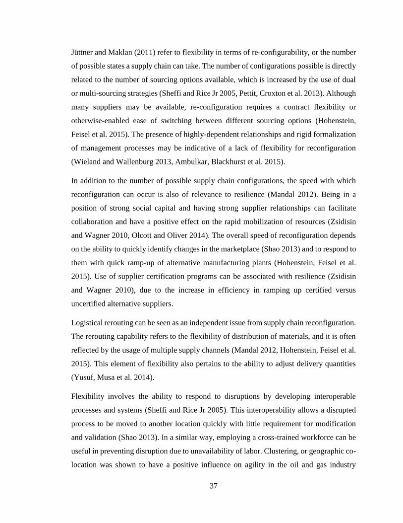
37
Jüttner and Maklan (2011) refer to flexibility in terms of re-configurability, or the number
of possible states a supply chain can take. The number of configurations possible is directly
related to the number of sourcing options available, which is increased by the use of dual
or multi-sourcing strategies (Sheffi and Rice Jr 2005, Pettit, Croxton et al. 2013). Although
many suppliers may be available, re-configuration requires a contract flexibility or
otherwise-enabled ease of switching between different sourcing options (Hohenstein,
Feisel et al. 2015). The presence of highly-dependent relationships and rigid formalization
of management processes may be indicative of a lack of flexibility for reconfiguration
(Wieland and Wallenburg 2013, Ambulkar, Blackhurst et al. 2015).
In addition to the number of possible supply chain configurations, the speed with which
reconfiguration can occur is also of relevance to resilience (Mandal 2012). Being in a
position of strong social capital and having strong supplier relationships can facilitate
collaboration and have a positive effect on the rapid mobilization of resources (Zsidisin
and Wagner 2010, Olcott and Oliver 2014). The overall speed of reconfiguration depends
on the ability to quickly identify changes in the marketplace (Shao 2013) and to respond to
them with quick ramp-up of alternative manufacturing plants (Hohenstein, Feisel et al.
2015). Use of supplier certification programs can be associated with resilience (Zsidisin
and Wagner 2010), due to the increase in efficiency in ramping up certified versus
uncertified alternative suppliers.
Logistical rerouting can be seen as an independent issue from supply chain reconfiguration.
The rerouting capability refers to the flexibility of distribution of materials, and it is often
reflected by the usage of multiple supply channels (Mandal 2012, Hohenstein, Feisel et al.
2015). This element of flexibility also pertains to the ability to adjust delivery quantities
(Yusuf, Musa et al. 2014).
Flexibility involves the ability to respond to disruptions by developing interoperable
processes and systems (Sheffi and Rice Jr 2005). This interoperability allows a disrupted
process to be moved to another location quickly with little requirement for modification
and validation (Shao 2013). In a similar way, employing a cross-trained workforce can be
useful in preventing disruption due to unavailability of labor. Clustering, or geographic co-
location was shown to have a positive influence on agility in the oil and gas industry

38
because of the increased skilled-labor pool in the industrial cluster (Yusuf, Musa et al.
2014).
Kleindorfer and Saad (2005) note that modular product design can be a key aspect in
achieving flexibility. If a component becomes temporarily or permanently unavailable, the
modular design may allow it to be easily replaced with a similar replacement component,
or to simply shift to production of parts with a slightly different end configuration. Agility
may be developed by use of postponement, a production strategy which delays final
customization of a product to the finishing processes, thereby affording the manufacturer
the ability to respond quickly to changes in demand for specific configurations (Pettit,
Croxton et al. 2013, Durach, Wieland et al. 2015). Similarly, the concept of product design
flexibility entails the use of new product introduction, slight design changes, and product
mix adjustment to meet the changing needs of the customer (Chiang, Kocabasoglu-Hillmer
et al. 2012).
Table B. 5: Elements of Flexibility, Velocity, and Agility in Appendix B summarizes
elements of flexibility, velocity, and agility.
2.2.6 Network Structure
The physical layout and characteristics of a supply chain network can have significant
effects on its resilience against disruptions. The descriptive elements of network structure
are closely tied to aspects of redundancy and flexibility, but are unique in their
consideration of the specific configuration of the nodes in the network. Elements that can
be used to differentiate different network structures include size, density, connectedness,
stability, and the criticality of individual nodes.
The element of network size generally refers to the number of suppliers or the supply chain
length (Blackhurst, Dunn et al. 2011). The number of nodes in the network has also been
referred to as node complexity (Adenso-Diaz, Mena et al. 2012) or network scale
(Brandon-Jones, Squire et al. 2014). Increasing numbers of suppliers can increase risk
exposure if not mitigated by other resilience-enabling factors.

39
Other network-related measures include density, or the number of connections that exist in
the network compared to the maximum number of connections it could possibly sustain
(Greening and Rutherford 2011). The geographic dispersion of the network represents the
spread of the network across different geographical regions. This spread can be useful in
terms of offering decentralization of key assets (Pettit, Croxton et al. 2013). However,
certain advantages may be available to organizations operating in geographical clusters
such as ease of communication, reduced transportation delay, and co-location of skilled
labor (Blackhurst, Dunn et al. 2011, Shao 2013, Yusuf, Musa et al. 2014).
The network can be described in terms of its flow complexity, measured by the number of
interconnections between nodes (Adenso-Diaz, Mena et al. 2012). Connectivity
distribution, a concept from complex network theory, describes the average number of
connections possessed by each node in a network and can be used to represent supply chain
connectedness (Hearnshaw and Wilson 2013). For example, a ‘scale free’ network implies
a system in which a small number of hub firms possess many connections while a much
larger number of peripheral firms possess few connections. An increase in connectedness
has a positive effect on resilience as this implies greater flexibility and collaboration among
firms.
Node criticality is an important measure which takes into account a variety of information,
and can be described as the importance of the node within a supply chain due to what it
does and what its relative contribution is to the overall realized value of the end product
(Craighead, Blackhurst et al. 2007). The replicability of the affected product, and the
degree of connectedness of the affected node all influence node criticality. Furthermore, if
a supplier with a high-power position is affected by disruption, the realized effects may be
greater implying greater criticality. Although the criticality of the node may be derived
mainly from non-network related variables, the position of a critical node within the
network can be of great significance if and when it is affected. The importance of a node
based on its network position can also be reflected by the metric ‘betweenness centrality’
which represents the node’s use as an intermediate connection (Basole and Bellamy 2014).
Geographic location of a node can also affect its strategic nature and therefore it can be an
important factor in supply chain resilience (Kovács 2009, Revilla and Sáenz 2014). Revilla

40
and Sáenz (2014) found though survey analysis that risk sources from natural hazards,
market, and socio-economic sources vary by region/country. For instance, the sub-Saharan
Africa region suffered more political and economic instability than other regions, and
natural hazard exposure varied by region depending on the type of hazard considered. In
contrast, the survey showed that the level of implementation of supply chain disruption
management practices was not dependent upon the region considered.
The overall network stability relates directly to the amount of time over which the network
has been established. As time progresses the supply chain network tends to evolve and
become more stable as buyer-supplier relationships are established and verified (Greening
and Rutherford 2011). The less volatile network is generally favorable for enabling
resilience.
Table B. 6: Elements of Network Structure in Appendix B includes the elements of network
structure extracted from literature.
2.2.7 Power and Dependency
Being in a low power position or a position of dependency can present difficulties for an
organization in the event of a disruption. Whatever the reason, this positioning inhibits the
ability of the supply chain to respond effectively after a disruption because of the reliance
on the affected node (Adenso-Diaz, Mena et al. 2012). A buyer may depend on its supplier
because the supplier controls an important resource that the buyer needs, because the
supplier is simply in a superior market position, or because the component being supplied
is strategically important.
In some cases, a supply chain member can exhibit high levels of control over a desirable
resource. The resource may be a highly specialized component, requiring significant
investment of time and resources for development of any alternate source (Ellis, Henry et
al. 2010, Pettit, Croxton et al. 2013). There may be few options for switching suppliers,
diminishing the negotiating power of the buyer (Greening and Rutherford 2011). In such
cases, it is common for a buyer to be forced to rely on a single-sourcing strategy (Adenso-

41
Diaz, Mena et al. 2012). Resource constraints should be identified through examination of
the supply chain network, including areas of typically low visibility such as 2nd and 3rd tier
suppliers.
If one company has a significantly higher market share or organizational strength, the less
powerful firm may be subject to the other’s demands (Peck 2005, Sheffi and Rice Jr 2005).
Determining the presence of such power dependencies requires examination of the relative
strengths of the buyer and supplier. Examples of ways in which these strengths may be
exhibited include customer loyalty, market share, and brand recognition.
In some cases, a buyer may be dependent upon a specific resource, simply because of its
strategic importance (Ellis, Henry et al. 2010). For example, the resource may represent a
large portion of the value realized in the end product. In this situation, a dependency may
result regardless of market conditions or the level of supplier control over the resource
supply.
Table B. 7: Elements of Power and Dependenc in Appendix B summarizes the elements of
power and dependency.
2.3 Incorporating Resilience-Enabling Factors in Segmentation
From the systematic literature review a variety of resilience-enabling factors that influence
supply chain performance were identified. The commonly used segmentation methods
were also reviewed to identify variables that are frequently used to group suppliers. A
closer review of the findings from these two studies reveals that many individual
segmentation methods may neglect resilience-enabling factors when assessing dimensions
used to group suppliers. For example, the portfolio method presented by Kraljic (1983)
uses two dimensions: complexity of supply market and importance of purchasing. It can
be argued that Kraljic’s two dimensions would also be influenced by a number of
resilience-enabling factors as shown in Figure 5.

42
Figure 2.7: Integration of traditional segmentation variables and resilience-enabling
factors
Thus, we postulate that by including a new set of resilience-oriented information, a
different perception of supply market complexity and purchasing importance may arise.
For example, the suggested factor ‘network connectedness’ may shed light on a
dependency in the network that exists with a certain supplier. Because this dependence is
made evident by the inclusion of the variable, the overall assessment of purchasing
importance may be higher than if the dependency had not been considered. Any of the
resilience-enabling factors could be potentially influential in the overall characterization of
the supply base. It is thus proposed that any resilience-oriented segmentation method
should consider some descriptive element of each of these main factors.
For further insight, the 161 segmentation variables from the studied segmentation methods
were examined in terms of their ability to reflect the resilience-enabling factors. Any
variables that could be used as an assessment of one of the resilience-enabling factors were
noted along with their category. In this way, it was possible to demonstrate which

43
resilience-enabling factors were best represented by the studied segmentation methods and
by which segmentation variable categories.
From this examination, it is shown that the resilience-enabling factors ‘visibility and data
analysis’ are fairly-well represented and are assessed primarily by the segmentation
variables for ‘supplier capability’. Visibility depends largely on the capability of the
supplier to collect data and convert it into usable information. The variables in the category
of ‘current relationship’ also relate to visibility, indicating a need for developing a
relationship with suppliers that fosters exchange of information.
Understandably, collaboration is reflected primarily by the ‘current relationship’ variables.
Although the segmentation literature reviewed does not represent an exhaustive list, it is
interesting to note that of the 161 examined variables there is no representation for the
specific collaboration elements ‘decision synchronization’ or ‘planning of employee
efforts.’ These elements of collaboration may be overlooked in existing segmentation
methods.
The resilience-enabling factor ‘training, learning, and business continuity planning’ is
overall poorly measured by the 161 segmentation variables. The variables that did represent
this factor centered on technical know-how at the supplier. Specific elements relating to
skills for recognizing risk, learning from past events and training simulations, and
developing and testing continuity plans are largely overlooked by segmentation variables.
The observations for this factor highlight the need for buyers to develop and include
variables for self-assessment regarding these skills.
The resilience factors for redundancy and flexibility have greater implications on day-to-
day operations, and thus are better represented by segmentation variables than other
factors. These factors are dependent on segmentation variables from all categories, with
redundancy being slightly more dependent on variables in the category ‘supplier
capabilities.’
Network structure is unique in that it appears as both a resilience-enabling factor and a
category of segmentation variables. The network represents the system in which all other
capabilities must be developed. Although both resilience and segmentation literature focus

44
on the size and dispersion of the network, the resilience literature introduces an additional
concept in the connectedness of the network. The number of connections in the network
may be more relevant after a disruption occurs and alternate production routes must be
established. A resilience-oriented segmentation should therefor include some assessment
for network connectedness.
The final resilience-enabling factor, power and dependency, is determined mainly by the
relative market strengths of the buyer and supplier. Notably, the nature of the product is
more relevant to power and dependency than any other resilience-enabling factor because
it is the importance and value of the product that gives significance to the control of its
production.
Development of a resilience-oriented supplier segmentation method will require a
resilience-assessment of buyer and supplier capabilities, buyer-supplier relationship,
product, and network. Current segmentation methods do not consider all factors of
resilience, but the examination of existing methods provides insight into the development
of a more exhaustive approach.

45
3 Methodology for Comparison of Segmentation Methods
The steps needed to assess the effectiveness of a supplier segmentation method for
enabling resilience and robustness are summarized in Figure 3.1.
Figure 3.1: Steps for assessing segmentation method
3.1 Phase I: Develop Revised Segmentation Method
For the purposes of this study, two dimensions and the resulting four supplier segments
described by Kraljic (1983) will be used in two supplier segmentation methods which are
to be compared. First, in the baseline method, only traditional variables are used to
characterize the suppliers on the two dimensions: complexity of supply market and
importance of purchasing. In the revised method, additional variables are used which are
not typically used in segmentation but have been identified in literature as having an
importance to supply chain resilience. The variables used to assess suppliers on the two
dimensions are shown in Table 3.1 and Table 3.2.
Descriptions are provided for each variable to guide the user in assigning values from 1 –
3. The number listed in the description are case specific, and should be modified to suit the
context in which they are applied. For example, in Table 3.1, ramp-up rate is subdivided
into categories of one month, one to three months, and more than three months. These
ramp-up lengths may or may not be appropriate depending on the product being
manufactured and their suppliers. The values 1 – 3 can be more generally interpreted as
low, medium, and high levels. A discussion and approval process should be undergone in
which these levels are defined. However, a clear distinction between levels is necessary so
that the users can answer consistently in case the assessment is repeated later or if multiple

46
respondents are consulted. The discussions held to define the categories for each variable
should focus on identifying the points at which the overall contribution to market
complexity changes significantly.
Scoring of each dimension is completed by summing the ratings for each variable. The
dimension is divided into low and high regions by dividing the range of the scores for each
dimension in half. If a supplier’s dimensional rating falls exactly at the midpoint, the
supplier is shifted into the segment corresponding to the higher value.
Table 3.1: Assessment variables for complexity of supply market
Baseline Variables
Additional Resilience-Oriented
Variables to be used in Revised
Method
Rating
Scale
Availability of
suppliers for
the
component
Entry Barrier:
time delay before
a new supplier
can be opened
Capacity
Utilization
Price
Volatility Ramp up rate
Variability in
transportation
delay
1
Many
suppliers
available in
the market
Short time delay
before opening
new supplier
(month)
Extra
capacity is
readily
available 0-5% 1 month
Less than 8
hours
2
Limited
number of
suppliers are
available in
the market
Medium time
delay before
opening new
supplier
(quarters)
Extra
capacity can
be made
available 5-10% 1-3 month
More than 8
less than 2
days
3
Single supplier
available that
can produce
the
component
Long time delay
before opening
new supplier
(over 1 year)
Capacity is
very limited;
difficult or
expensive to
expand 10-15%
More than 3
months over 2 days

47
Table 3.2: Assessment variables for importance of purchasing
Suppliers are classified as strategic, leverage, non-critical, or bottleneck. Once each
supplier has been associated with one of the four segments, an appropriate procurement
strategy should be assigned. Suppliers that fall in the range of higher market complexity,
strategic and bottleneck, are typically managed with frequent collaboration and
information sharing. Fast-response mechanisms should be put into place in the event of a
disruption at one of these suppliers. The level of strategic importance also affects such
decisions as how much buffer inventory to hold for each component, and whether to use a
dual or multi-sourcing strategy. Although the procurement strategies for each segment can
be described with detail, the study is limited by the requirement that such strategies must
be operationalized and assigned to many suppliers in the simulation. The aspects of strategy
that could be included in the simulation for each segment are summarized in Table 3.3.
Baseline Variables
Additional Resilience-Oriented
Variables to be used in Revised
Method
Rating
Scale
Component criticality to
end-product
quality/performance/dist
inguishability Cost/Unit
Transport
Cost/Unit
Cost per
unit
difference
during
disruption
and
recovery
Connectedness:
# of incoming and
outgoing
connections
1
Could be replaced or
substituted without
significant change
Lower 1/3 of
all purchases
Proportional to
distance, lower
1/3
The same or
less than
standard
cost
Low # of
Connections (1-2)
2
Customer may notice
some change in if
component is replaced or
substituted)
Middle 1/3
of all
purchases
Proportional to
distance, middle
1/3
slightly more
than
standard
cost (1 - 2X)
Medium # of
connections (2-3)
3
Replacing or substituting
component will cause an
obvious change
Upper 1/3 of
all purchases
Proportional to
distance, upper
1/3
significantly
more than
standard
cost (> 2X)
High # of
connections (>3)

48
Table 3.3: Procurement strategies for each supplier segment
3.2 Phase II: Framework for Comparative Analysis
In practice, the segmentation process should act to reduce the requirement for complex
systems modeling and analysis. In the ideal case, the assessment should indicate an
appropriate strategy for each supplier without need for further confirmation. However, for
the purposes of this research a modeling and simulation paradigm is needed to assess the
supply chain performance after being segmented with the baseline and revised strategies.
A discussion of various modeling and simulation paradigms available and their usefulness
in different contexts is presented in chapter 4.
In this work, the Agent-Based Modeling and Simulation (ABMS) paradigm is used to test
the supply chain’s resilience and robustness to different disruption scenarios. The
justification for using the ABMS paradigm is also outlined in chapter 4. Once the
disruptions have been implemented, the resulting resilience and robustness can be
observed, in addition to the normal operating range for KPIs.
3.3 Phase III: Application to Case Study
The segmentation method must be assessed in the context of a supply chain, which requires
the specification of an end-product and its bill of materials. A subset of the entire bill of

49
materials can be used as required for complexity reduction. Furthermore, the network of
suppliers from which the raw materials and sub-assemblies are procured must be defined
and organized into a network structure. Data is then collected regarding the different
suppliers’ characteristics. The data needed is defined by the user and is to be used in the
segmentation process. Based on the available data, the suppliers are then characterized
according to the predefined segmentation process. A complete description of the case study
employed in this work is presented in chapter 5.
3.4 Phase IV: Analysis of Results
Output data is to be collected from the ABMS for KPI after segmenting the supply chain
with each method. For each method, different disruption scenarios are studied that are
differentiated by their points of origin within the network. Furthermore, the disruptions are
implemented with two different start times and two different severities. The disruption start
time occurs either in the second or fourth quarter of the year. The severity is either a 50%
or 100% loss of production capacity. The combination of two levels for severity and start
time requires four disruption scenarios to be analyzed for each point of origin and each
segmentation method.
The robustness and resilience are assessed by first observing the supply chain during its
normal operating conditions. The normal operating range for inventory levels at the
distribution centers (DCs) is determined for each quarter of the simulation runtime. The
types of inventory that are observed include final assembly, photoconductor, and cartridge
assembly. The total supply chain cost is also determined for each quarter. Robustness can
then be measured as the maximum deviation that occurs from the normal operating range.
Resilience is assessed as the total amount of time the metric falls outside the normal
operating range.
A set of hypotheses is developed regarding the expected behavior of the KPI during the
various simulation scenarios.

50
a) The revised segmentation method will increase resilience of the supply chain
compared to baseline method.
The revised segmentation method incorporates additional information that is
shown by literature to have a direct connection to resilience. The incorporation
of the new variables does not necessarily indicate that more or fewer suppliers
will fall into any one segment. Rather, the new information creates a tendency
for suppliers with a strong potential to create significant disruption impact to be
separated and segmented differently from suppliers with a weaker potential for
creating a large impact. Making use of information pertinent to supply chain
resilience increases the likelihood that suppliers with similar needs for
resilience and robustness will be grouped together.
b) A disruption at a strategic supplier is likely to have a more severe impact on the
supply chain than a disruption at a non-critical supplier. The impact after a
disruption at bottleneck or leverage suppliers is likely to fall into a middle range
of severity.
This hypothesis is based on the idea that a supplier with higher strategic
importance and a more complexity in the market will be more likely to create a
high-impact disruption. Non-critical suppliers have the lowest market
complexity and importance of purchasing. Bottleneck and leverage suppliers
have a mix of high and low market complexity and importance of purchasing.
c) Disruptions that start during a period of high demand are likely to have a
stronger impact than those that occur during normal demand periods.
Most of the KPI used to assess resilience and robustness are related to inventory
and material flow. Production capacity is more constrained during periods of
elevated demand. If the production capability is diminished at a time when it is
under high demand, there is a greater likelihood that the need for production
will exceed available resources.

51
d) Disruptions that cause a greater reduction in production capacity will have a
greater impact on the supply chain.
As with the previous hypothesis, the production capacity is necessary to
maintain the desired inventory levels. If the capacity is 100% depleted in a
disruption, it will take longer for the resources to return to their original state
than if the capacity were only reduced to 50%.

52
4 Analysis and Selection of Modeling and Simulation Paradigm
The modeling and simulation paradigm used to assess the behavior of the supply chain
should be chosen carefully according to the needs of the study. The objective of this section
is to examine the primary modeling and simulation paradigms that have been used to
represent supply chains. These methods are discussed regarding their convenience toward
answering different types of questions. The paradigms that will be discussed include
Discrete Event Simulation (DES), System Dynamics (SD), and Agent-Based Modeling and
Simulation (ABMS). A survey of different modeling approaches is described by North and
Macal (2007). A representation of the Beer Game is constructed using each modeling
approach in the attempt to highlight the differences in model structure which can all be
used to represent a similar phenomenon. In the work, it is noted that each modeling
paradigm can be differentiated according to its primary element of focus. For example,
when constructing a DES representation of a system, the primary focus is on describing
the individual processes and variability associated with those processes. In an SD model,
the focus is on high level system behavior as defined by a set of stock variables and their
change over time. ABMS focuses on representing the decision-making rules that exist
within the system. The methods can also be differentiated by their representation of time,
as each is able to capture the dynamic evolution of the system in a unique way. Finally,
some questions which are particularly well-suited for each paradigm are described. These
descriptions are collected in Table 4.1.

53
Table 4.1: Modeling Paradigms
Discrete Event Simulation
(DES) System Dynamics (SD) Agent-Based Modeling and Simulation (ABMS)
Primary Elements Process and Variability Stock and Flow Variables Decision-Making Units (Agents)
Time Representation Discrete points at which events occur
Constant increments Constant increments
Appropriate Questions What are the effects of increasing/decreasing process variability? Estimate flow times, wait times, etc.
What are the long-term trends given a range on external conditions? How to avoid unintended system behavior?
What is the emergent behavior of a group of autonomous decision makers?
ABMS appears to offer the most promising capability because the objective of the proposed
research is to study the effect of individual behaviors at suppliers, manufacturer, and
distributor. In chapter 5 of Managing Business Complexity, North and Macal (2007) list a
number of characteristics of problems suited for ABMS. From the list of characteristics,
the ones aligned most with the requirements of the supply chain problem are the following.
1. When it is important that agents adapt, and change their behavior.
2. When it is important that agents have dynamic relationships with other agents, and
agent relationships form and dissolve.
3. When it is important that agents have a spatial component to their behaviors and
interactions.
4. When process structural change needs to be a result of the model, rather than an
input to the model.
Together these features justify the use of ABMS for the purpose in the proposed context of
modeling disruption impact under different procurement strategies. Given the choice of
ABMS as a modeling and simulation paradigm to be used in the remainder of the work, it
is pertinent to provide a review of ABMS and its uses with a focus on supply chain
applications.

54
4.1 Agent-Based Modeling and Simulation
The origins of Agent-Based Modeling and Simulation (ABMS) are in the field of complex
adaptive systems (CAS), which is primarily focused on examining the adaptive
mechanisms of biological systems (North and Macal 2007). In CAS, individual elements
of the biological system respond to a changing environment to increase their chances of
survival. Over time the field of CAS expanded from its early focus on biology into other
areas such as network, social, and systems science, leading to the current field of ABMS.
Since its development many types of problems have been studied using ABMS, including
the flow of crowds during evacuations, predator-prey population dynamics, and cellular
systems (North and Macal 2007). ABMS is related to but should not be confused with
Multi-Agent Systems (MAS) which is based on solving problems related to the interaction
of machines and designing agents to solve specific problems. An MAS tends to be
normative, where the machines are designed to complete an objective, whereas ABMS is
typically descriptive, and used to examine patterns of behavior that emerge in a complex
system of autonomous agents (North and Macal 2007). In large part, ABMS is
distinguished from MAS because of its background and relation to social systems and use
for behavioral observations.
A simple example which demonstrates emergent behavior of agents is known as the Boids
simulation, which imitates the flocking behavior of birds using agents with a set of only
three rules (Zsidisin, Melnyk et al. 2005, Reynolds). First, the rule of cohesion dictates that
each agent (or bird) should move towards the average position of its surrounding “flock-
mates.” Next, a separation rule is applied so that the birds will avoid overcrowding. Finally,
an alignment rule dictates that each agent should orient itself toward the average direction
of those in a specified surrounding area. Based on these simple rules applied only at the
individual agent level, a systematic flocking behavior emerges wherein it appears that the
birds share a common objective, or heading.
ABMS is an object-oriented technique which can be used to study the behavior of complex
systems by focusing on the individual decision making units, or agents, upon which the
system is built (North and Macal 2007). Each agent-based model consists of a set of agents,
which are described by Lee and Kim (2007) as problem-solving entities that act through

55
autonomous rule-based reasoning. Agents respond to environmental conditions, and send
and receive messages to other agents regarding their current situations. Each agent contains
a set of attributes and behaviors, and can relate to other agents and the surrounding
environment (North and Macal 2007). Agents can conduct interactions in either a co-
operative or self-interested manner. Unlike in a traditional optimization model, there is no
centralized objective. Rather, ABMS is used to reveal emergent trends based on the
specified behavior of the individual agents.
Agents can be classified into three types of architecture: reactive, deliberative, and hybrid
(Forget, D’Amours et al. 2008). Reactive agents link specific inputs to specific outputs,
meaning that if the agent observes an environmental condition, then it has a pre-specified
action. This is the simplest of the three architectures and is characterized by a lack of
adaptability. Deliberative agents use the knowledge gained from environmental
observations combined with internal goals to execute their actions. This allows the agents
to make decisions suited for the approach of long-term goals. In dynamic environments,
the time needed for the agents to process the information and act on it can be important.
Agents need to be able to make informed decisions before the environmental conditions
change. Hybrid architecture uses a layering technique to gain some of the advantages of
both reactive and deliberative agents. First, the agent will observe the environment and
determine if there is an existing behavioral response for the situation. If there is no known
response, the agent deliberates to try to find an action that will solve the problem. If the
agent cannot find a solution to the problem, it will collaborate with the other agents to find
a feasible solution.
Collaboration between agents is relevant to the study of SRM, and it is important to
understand the various modes of inter-agent collaboration if the strategies of SRM are to
be represented in a supply chain simulation. Methods used to facilitate cooperation among
supply chain agents have been categorized by de Santa Eulalia (2009). These methods are
summarized in the following paragraphs.
Communication - describes the conveyance of information between agents.
Communication can be direct or indirect, such as through a universal access point. Other
questions include whether the information exchange is synchronous or asynchronous, how

56
many agents will receive information, whether there is human participation, and what the
sending and receiving rights of the agents should be. There may be security mechanisms
in place such as required authentication to prevent leaking of confidential information.
Grouping and multiplication - relates to the forming of agent coalitions to solve
problems. One example is agent cloning to allow parallel computation. The agents group
together for concurrent information processing.
Coordination - mechanisms used to manage dependencies in activities. This facilitates
agent interaction in a way that leads to an overall solution and prevents chaos. Different
coordination frameworks include direct supervision during activity execution, mediation
during activity execution, mutual adjustment during activity execution, direct supervision
with plan, mediation with plan, joint plan establishment, coordination by standardization,
coordination by reactive behavior, synchronization, and coordination by regulation.
Collaboration - a group of agents work together on a common task by sharing tasks and
resources. Tasks are decomposed into subtasks and then resources are allocated to the
subtasks. The decision can be centralized or distributed.
Conflict resolution through negotiation and arbitration - mechanisms used to resolve
conflicts of resource allocation. Negotiations can be bi-lateral or multi-lateral. Arbitration
can be used which requires an impartial third party referee, agreed to by all agents involved
in the dispute. Arbitration is suited for reactive agents, while negotiation is mainly
associated with deliberative agents.
ABMS has been demonstrated in the context of supply chains, and may prove to be
especially beneficial when different entities in the supply chain act in their own self-
interest. A representation of the existing work in applying ABMS techniques to supply
chain problems is provided in Section 4.2. As demonstrated in the examples, the ability to
allow agents to make autonomous decisions based on their internal objectives is a key
feature of ABMS that makes it well-suited for modeling the complexity of supply chain
interactions.

57
4.2 Supply Chain Applications of ABMS
One of the earliest uses of intelligent agents to represent the supply chain was presented by
(Fox, Chionglo et al. 1993). The work was in response to the company’s desire to rely less
on rigid planning and to allow faster responses to changes in the system such as demand
variation and late deliveries. The authors divide supply chain management activities into
three levels: strategic, tactical, and operational. The article highlights the important issues
of determining how to distribute supply chain activities among agents, establishing how
the agents interact to arrive at mutually acceptable solutions, the time required for an
algorithm to come up with a response to a given situation, and knowledge availability. The
agent architecture used consists of functional agents, which plan and control activities, and
information agents, which assist the functional agents by providing communication. The
six functional agents used are logistics, transportation management, order acquisition,
resource management, scheduling, and dispatching. A graphical depiction of the agent
interactions is shown in Figure 4.1.
Figure 4.1: Supply chain agent interactions, (Fox, Chionglo et al. 1993)

58
The logistics agent tries to ensure on-time delivery at minimum cost. As input, it receives
orders from the order acquisition agent, and outputs production and transportation
requirements. The transportation management agent assigns and schedules transportation
resources taking into consideration different assets and routes. The order acquisition agent
negotiates price and due date with the customer, and forwards order information to the
logistics agent. The resource management agent generates purchase orders and manages
inventory. The scheduling agent schedules activity in the factory based on order
information received from logistics, resource problems from resource management, and
schedule deviations from dispatching. Finally, the dispatching agent performs real time
order release and floor control.
The model presented by Fox, Chionglo et al. (1993) provides a good foundation for
understanding the capabilities of ABMS in the supply chain context. To better reveal
additional capabilities, a literature review was conducted specifically to uncover examples
of ABMS for supply chain with a special emphasis on understanding and categorizing the
methods of representing the relationships between supply chain entities. A search was
conducted using the Compendex and Business Source Complete databases. Search terms
included are shown in Figure 4.2.

59
Figure 4.2: Supply chain ABMS search terms
Related terms are shown within the boxes. To conduct the search “or” statements were
used between related terms and “and” statements were used between categories. This
approach should result in articles concerning supply chain applications of ABMS.
Furthermore, the results should include one or more of the terms in the third category which
includes resilience-enabling (or disenabling) factors which were identified in the
previously conducted literature review described in Section 2.2.
Examination of the resulting articles will begin with a look at a small subset of the articles
which consider modeling of disruptions. The purpose of this initial focus is to highlight

60
the ways in which resilience or robustness has been measured. The review should examine
how the disruptions themselves are represented and identify any variables that might
mediate the effects of disruption.
One study examined the effect of the network characteristics on the robustness against
disruptions (Nair and Vidal 2011). Network characteristics included were average path
length (the average distance between any pair of nodes in the network), clustering
coefficient (relates the probability that the two nearest nodes are connected), and largest
connected component (the size or number of components in an isolated sub-cluster of the
network and the maximum distance between nodes in the sub-cluster). The performance
measures examined as an indication of robustness are inventory level, backorders, and total
cost. Two network topologies are considered. Scale-free topology indicates that nodes
exhibit preferential attachment logic while random topology indicates random attachment
of nodes with no specific preference. Findings indicate that long average paths between
nodes in the network are detrimental to robustness. Clustering of the nodes within the
supply chain network can increase the efficiency of operation, but these advantages should
be balanced with the adverse effects to disruption response. The authors warn that various
performance metrics need to be considered to fully understand the effects of the network
topology on robustness. A limitation of the study is that it does not allow for re-
configuration or adaptation in the network after a disruption occurs. Also, the potential
benefits of building up and maintaining a buffer inventory at certain potentially vulnerable
facilities is not considered. In the model, the disruptions occur at random based on a given
probability, with three levels of likelihood examined. The model also considers targeted
attacks. The severity of the disruption is measured in terms of the length, 1-3 weeks. All
the facilities are considered agents as well as the customers modeled by a random demand
function. Decisions made follow a similar format to the beer distribution game (Sterman
1989), with each entity deciding what orders to place in each iteration.
Another ABMS studies a disruption at the retailer (Wu, Huang et al. 2013). Input variables
include the stockout length at the retailer for different products and the initial market share
of the retailers and products. The response variable considered is the market share after the
stockout. The purpose of the model is to study the impact of the stockout at the

61
manufacturer and retailer. Agents are defined as retailers, manufacturers, and consumers,
where consumers are classified as brand-loyal, habitual, or not loyal. Consumer decisions
allowed in the model include purchasing products at another store when the preferred store
is stocked out, delaying purchase to a later time, substituting with the same brand,
substituting with a different brand, or not purchasing at all. The strength of this model is
its allowance for different consumer response profiles based on market research. The
agents can make autonomous decisions much like in a real system, and the agents’ decision
making rules can adapt over time. Different stockout lengths are considered. Resilience is
measured in terms of the change in market share for both manufacturer and retailer.
Different product types are considered having different customer response profiles. Also,
different initial market shares are considered for the retailers. It is shown that the
manufacturer and retailer may find mutual benefit in directing their attention to satisfying
the right kinds of customers who have the most impact on market share and by focusing
on products that have a high level of loyalty associated with them.
There is a need to integrate modern IT systems into a framework for developing agent-
based decision support systems for handling disruptions in the supply chain (Giannakis and
Louis 2011). A literature review was conducted to support the development of a framework
for a disruption management system. The article focuses on the disruption management
part of the framework, which is designed to initiate collaboration between agents when a
potential problem is detected. Separate agents are proposed for communication,
coordination (operating within the individual organizations/facilities), monitoring
(watching the production schedule and triggering warnings), wrapper (facilitating
information exchange from legacy systems like ERP and other agents), and disruption
manager (proposing solutions to the problem at hand, considering past approaches for
similar problems). The agents cooperate to detect the problems and convey the information
to the disruption manager. Risk identification comes from regular monitoring of KPI’s,
such as inventory, throughput, utilization, and delivery lead time. Aberrations from normal
level indicate a disruption is present. This result provides a good follow up to a survey
paper published in 2006 on the use of ABMS in manufacturing (Shen, Hao et al. 2006). A
key takeaway from the work is the suggestion that future work in the area should focus on
integrating agent-based planning and scheduling systems with existing systems, such as

62
real-time data collection systems, Enterprise Resource Planning and Material
Requirements Planning.
Li and Chan (2012) examine collaborative transportation management (CTM) in handling
demand disruptions. The aim of the research study was to find out what possible side-
effects CTM might have on risk, as it is originally designed to increase efficiency. In the
model, demand has a normal distribution and in the disrupted state is represented with a
shift in the original distribution. The manufacturer gets demand data from the retailer and
uses that to establish a re-order point, rather than relying on the retailer to place orders. In
this way, CTM changes the information sharing and cooperation relationships of the
involved parties. The CTM system is shown to improve response to demand disruptions
specifically by reducing cost and adding flexibility. CTM has the intended purpose of
making transport planning and execution more efficient. Each company in the model is
simulated by an agent. The model includes stochastic demand, one retailer, one transporter,
and one manufacturer. Performance is measured in terms of supply chain profit and cost,
retailer’s inventory, and transporter’s delivery ability. Limitations noted in the paper are
the inability to handle other types of risk including financial, supply, and information risks.
Only the total profit of the supply chain is considered. Ultimately, it was concluded that
supply chains implementing CTM could handle demand disruptions better than those
without CTM.
Also focused on the area of demand disruption, but still providing insight into ABMS
applications for supply chain disruption is the article by Upton and Nuttall (2014) that
relates to fuel panic buying. The work offers a model to inform policy makers during such
periods of demand disruption. The value of this work is the demonstration of the methods
of information sharing to control the panic response. The model tries to reproduce transient
behavior observed in past fuel panics. The closing of refineries and subsequent cut off
supply resulted in panic buying and accelerated depletion of existing inventory. Twelve
years after the initial panic event, the possibility of a strike was rumored, and panic buying
again began, this time fueled by political statements. Even though no strike ever occurred,
panic buying did ensue. In this instance the effect of the initial panic was different partly
because of the prevalence of information about the event via the internet. Agents in the

63
model represent vehicles with a stated fuel tank capacity. They must travel to pre-stated
destinations, consuming fuel in the process. A social network overlays the physical system
and the agents communicate with each other regarding their state of panic or lack thereof.
The decision to panic or not is also related to the size of queue at each filling station. The
system is tested by putting all the agents into a state of panic for 300 time units. An agent
in the panic state chooses to top off the fuel after any trip. This ultimately leads to an
oscillatory behavior as cars maintain close to full capacity until the period of panic ends,
and then essentially synchronize their demand cycles. The consensus from the work is that
the spread of information is important in modeling the effect of disruption. How the agents
interact will largely dictate the result. Many metrics can be used to provide an indication
of the system’s resilience.
The next article is highlighted for its discussion of performance assessment in the supply
chain (Behdani, Lukszo et al. 2010). As noted in the article, the entities in the supply chain
form a socio-technical system wherein physical and social networks act together.
Achieving the optimal system level goal for the supply chain does not necessarily mean
that each local goal can be achieved. Incentives may be provided to persuade individual
entities to pursue system-level objectives. Specifically, the paper provides an illustrative
example using the model to study the effects of a plant shut down. Recovery policies
involve changing the re-order points at the other two remaining facilities, or rejecting some
orders if they are not from important customers. These policies have different effects on
the number of late orders, total tardiness, and total profit. The model can also be used to
process negotiations, such as when the order cannot be delivered on time. Instead of just
notifying the customer that the order cannot be fulfilled, the customer and facility agents
negotiate on a new due date and possible price reduction.
Figure 4.3 demonstrates a summary of topics synthesized from the initial literature search.

64
Figure 4.3: Focus areas within literature on ABMS supply chain applications
Of these results, methods of collaboration between entities in the supply chain are of
relevance to the proposed work, and many articles were retrieved in this subject. Other
topics of prominence which arose include visibility and flexibility which relates to the use
of alternative supply configurations. Because collaboration is particularly well-suited for
modeling by interacting agents, and has a direct connection to supplier relationship
management, the remainder of the review will focus on a subset of articles published in
this area.
Hou, Sheng et al. (2008) study the benefits realizable from the formation of alliances
between buyers and suppliers. Some potential benefits include shared financial risk and
reduced costs, innovative product development, and resolution of competitive conflicts.
The authors argue that the de-centralized control of agents offer better representations of
supply chains than traditional operations research methods. The agent-based model studies
the effect of myopic behavior at a retailer on the supply chain alliance by allowing the
retailers to base purchasing decisions on either long or short-term revenues and by allowing
retailers to vary supplier switching probabilities. The model also considers the number of
retailers in the market and length of order lead time. Results indicate that myopic decision
0
5
10
15
20
25
30
35
# o
f ar
ticl
es

65
making by the retailer reduces the overall profitability. In the competitive environment
with more retailers, this effect is even stronger. The comparative benefit of long-term
decision making diminishes but remains favorable as order lead time increases.
Mohebbi and Li (2012) examine long-term partnerships in e-supply networks (e-SNs).
Qualified partners are selected. Both buyer and supplier should benefit from long-term
multi-period exchanges. The development of e-supply networks facilitates real time
decision making. Membership in the supply chain exhibits flexibility. The e-SN system
takes an ebay-like approach in that the suppliers pay a fee to exist on a site and buyers can
leave ratings based on their experiences with suppliers. Agents can facilitate the sharing of
information vertically while preventing access to intellectual property.
Distributed operations planning was examined for the softwood lumber supply chain
(Gaudreault, Forget et al. 2010). The agent model is used to plan and schedule the
operations within the supply chain. The plans of the different agents are then coordinated.
Coordination in this context means that the individual entities should plan with
consideration of dependencies on other operations. Within a single plant, coordination
across the function of production and supply, production and distribution, and inventory
and distribution. This is inter-functional coordination. Coordination also occurs across
plants for the same function.
Albino, Carbonara et al. (2007) note most work that has been conducted in studying
cooperation in supply chain has been qualitative and has adopted the perspective of large
companies as buyers cooperating with their suppliers. The paper focuses on cooperation
within Industrial Districts (ID) which are collections of small and medium sized firms
acting in a network of buyer-supplier relationships in both competitive and cooperative
nature. The type of cooperation examined in the study has the aim of balancing production
capacity utilization while minimizing unsatisfied customer demand. The benefits of
cooperation are studied under different demand uncertainties and organizational structures
(presence of one or more leader firms in the ID). Results indicate that the benefits of
cooperation increase when the demand variability is high because of the balance of
flexibility and efficiency. The existence of leader firms can result in a reduction of overall

66
flexibility in the ID, especially if the leader firms utilize their extra bargaining power. This
is an interesting study that focuses on a single type of cooperation.
ABMS is used to evaluate the value of cooperation (Janssen 2005). A semi-cooperative
structure is examined wherein the agents optimize the supply chain while at the same time
trying to maximize their own goals. Production agents try to optimize their resource
utilization. DC agents try to balance supply and demand, minimize the amount of inventory
and reduce stockouts throughout the entire supply chain. Dealer agents try to minimize
their individual number of stockouts. The study showed that using the multi-agent approach
to determine the amount of inventory to deliver during specific periods from the DCs
increased the ability of the supply chain to respond to high volatility of demand.
Autonomous Cooperation and Control (ACC) is assumed to create strategic flexibility
(Hulsmann, Grapp et al. 2008). This paper is not about agents per se but focuses on
explaining why ACC can provide competitive advantage to the global supply chain. It notes
that logistics systems using ACC handle complexity and dynamics more effectively than
those that do not. Strategic adaption is the primary mechanism by which the paper suggests
competitive advantage can be gained. The systems should be able to take in new
information and adjust based on this, but not compromise stability by changing too much
with every slight change in input. ACC is a system of decentralized decision making.
Compared to a system working toward a centralized objective, ACC has the advantage in
terms of flexibility.
Collaborative planning forecasting and replenishment (CPFR) is a process in which trading
partners exchange sales information and forecasts (Caridi, Cigolini et al. 2005). The study
examines the ability of intelligent agents to improve the negotiation process involved.
Three negotiation models are studied: the original CPFR method, an advanced model using
agents, and a learning model using agents. Metrics used to measure the improvement are
cost, inventory level, stockout level, and sales. CPFR is a 9-step framework for buyer-seller
exchange of sales and forecast data on a web-based platform. The negotiations are designed
to handle situations where the sales forecast at the buyer and seller differ, or when the order
forecast at the buyer differs from the seller’s ability to supply. When an exception to the
forecast happens, the agreement must be re-negotiated. This effectiveness of negotiations

67
from the different models controls the reduction of bullwhip affect when something
unexpected happens and can reduce lost sales.
Articles presenting collaboration-oriented ABMS models can be differentiated by the
cooperation goal, the method in which cooperation between agents is represented, the
external factors that are considered, and the metrics used to measure the effectiveness of
cooperation. Cooperation goals include minimization of unsatisfied customer demand or
stockouts (Janssen 2005, Albino, Carbonara et al. 2007), reduction of forecast
discrepancies (Caridi, Cigolini et al. 2005), and cost minimization (Gaudreault, Forget et
al. 2010). Methods of collaboration include enhanced communication both horizontally
between suppliers and vertically up and down the supply chain. External factors considered
include demand uncertainty, forecast uncertainty, and available production capacity and
utilization. Effectiveness of collaboration can be measured in terms of flexibility or
efficiency of operations, lead times, stock levels and number of stockouts, total cost, and
on-time delivery percentage.

68
5 Case Study
An illustrative case study presented in this section will be used to demonstrate the
application of ABMS to model disruption behavior. The context of the case study is a laser
printer supply chain, based on a combination of information provided by an industry
partner and public information about the components of a laser printer. Many of the
components to be considered in the supply chain case study are demonstrated in Figure 5.1.
Figure 5.1: Laser printer components (Oki Data Systems 2007)
5.1 Laser Printer Bill of Materials
The case study need not consider a comprehensive list of components for the laser printer.
Rather, components are selected to demonstrate a multi-tier supply chain with enough
complexity to warrant the need for segmentation. The example will include one facility for
final assembly and several regional DCs. Component suppliers are included through the
second tier, and both internal facilities and contract manufacturers are included. Figure 5.2
demonstrates the simplified bill of materials for a laser printer to be used in the case study.

69
Figure 5.2: Laser printer tiered bill of materials
The printer cartridge assembly consists of the toner itself, plastic parts which make up the
structure of the cartridge, and gears. Plastic parts and gears are separated into type one
which goes into the final printer assembly and type two which goes into the cartridge
assembly. The Printed Circuit Board Assembly (PCBA) includes as subcomponents the

70
display panel and Application Specific Integrated Circuit (ASICS). The Laser Scanning
Unit (LSU) consists of the laser, a lens, and movable mirror used to maneuver the beam to
write the electrostatic image onto the photoconductor. For simplicity purposes the
subcomponents of the LSU are not included. Components which are commonly purchased
aftermarket by the end user are the toner cartridge and photoconductor. These components
are placed near their demand centers to improve customer responsiveness and each is
manufactured in two locations. Other components included in the study are the fuser, which
is used to heat and melt the plastic component of the toner, causing the image to be
permanently fixed on the page. DC motors are used to power the rollers for paper transport,
and the power supply converts electricity to DC for the electronic components. The scanner
refers to the document scanner that sits on top of the main printer assembly. The above
components represent a simplified version of a laser printer broken down into some of its
key components.
5.2 Data Collection
Data for the printer supply chain was collected through a combination of meetings with
supply chain professionals at a consumer electronics manufacturer producing laser printers
and toner cartridges and research of publicly available information.
A presentation was provided by the company in which the general structure of the global
supply chain network was outlined as seen in Figure 5.3. The printer case study that forms
the context for the ABMS is based on the initial presentation and follow-up interviews with
the company.

71
Figure 5.3: Global operations for laser printer supply chain
Basic understanding of the laser printer components was developed and from this a
potential BOM and supply chain configuration were presented to the industry partner. After
a few iterations, the simplified BOM presented in section 5.1 was agreed upon along with
the network structure and spatial representation demonstrated in
Figure 5.4. The arrows connecting the suppliers in the figure are scaled in proportion to the
transportation delay between nodes. In the ABMS paradigm, each complete iteration of the
simulation procedure is counted as a tick. The simulation is designed such that each tick
corresponds to a simulated hour. The longest transportation delay of 16 ticks, or 16
simulated hours, is shown with the red arrow, and so on with the blue and green arrows.
The industry partner was presented with a set of tables (Table 3.1 and 3 from chapter 3)
containing a list of assessment variables and a suggested 1 – 3 rating scale with verbal

72
descriptions of the meaning behind each rated value. The supplier for each component in
the BOM was assessed based on prior experience from the supply chain managers.
Figure 5.4: Spatial representation of laser printer supply chain
Cost data for each component was first estimated based on publicly available information
and then presented to the industry partner to check validity. The information collected was
then used to rank each supplier on the two dimensions: complexity of supply market and
importance of purchasing (Kraljic 1983). This data would also be included in the
simulation as defining characteristics for each supplier. Response data for market
complexity for the ranked assessment of each segmentation variable is presented in Table
5.1. The summed scores for market complexity are provided for the baseline method and
the revised method which incorporates two new variables. Similarly, the response data for
purchasing importance is presented in Table 5.2.

73
Table 5.1: Variable assessment for market complexity
Baseline Assessment Variables Additional Resilience-Oriented Variables
Supplier
Availability of suppliers for
the component
Entry Barrier: time delay
before a new supplier can be opened
Capacity Utilization
Price Volatility
Baseline Total
Ramp up rate (after opening, how fast does an alternate
ramp up to full capacity, and how
fast does a disrupted supplier ramp up in
recovery)
Logistics variability (variability in
transportation delay)
Revised Total
Plastic parts 1 2 1 1 5 1 1 7
Packaging materials 1 1 1 1 4 1 1 6
Displays 1 2 1 1 5 2 3 10
ASICS 2 3 2 1 8 3 3 14
LSU 2 3 1 1 7 3 2 12
Gears 2 2 1 1 6 1 1 8
Toner 3 3 1 1 8 3 3 14
Power Supply 2 3 1 1 7 2 1 10
DC motors 1 2 1 1 5 2 1 8
Fuser 2 3 2 1 8 3 1 12
PCBA 1 2 1 1 5 2 2 9
Cartridge Assembly 2 2 1 1 6 1 1 8
Scanner 2 3 1 1 7 2 1 10
Photoconductor 3 3 1 1 8 3 3 14

74
Table 5.2: Variable assessment for purchasing importance
Baseline Assessment Variables Additional Resilience-Oriented Variables
Supplier
Component criticality to end-
product quality/performance/distinguishability
Cost/Unit
Normalized Cost/Unit
Transportation
Cost/Unit
Baseline Total
Cost per unit
difference during
disruption and
recovery
Connectedness: # of incoming and outgoing
connections
Normalized Connectedness
Revised Total
Plastic parts 1 12 1 1 3 1 3 2 6 Packaging materials 1 10 1 1 3 1 1 1 5
Displays 1 30 1 1 3 2 1 1 6
ASICS 1 30 1 1 3 2 1 1 6
LSU 1 25 1 2 4 2 1 1 7
Gears 1 3 1 1 3 2 3 2 7
Toner 1 50 2 3 6 2 2 1 9
Power Supply 1 30 1 1 3 2 1 1 6
DC motors 1 5 1 1 3 2 1 1 6
Fuser 1 50 2 1 4 2 1 1 7
PCBA 1 100 3 2 6 2 3 2 10 Cartridge Assembly 1 60 2 1 4 2 7 3 9
Scanner 1 120 3 1 5 2 1 1 8
Photoconductor 1 50 2 3 6 2 4 2 10

75
Scoring of purchasing importance required normalization on the 1-3 scale for cost/unit,
which was estimated in dollars, and connectedness, which was counted as the number of
incoming and outgoing connections at a node. Scaling was performed by simply dividing
each reported value by the highest reported value for the variable, multiplying the ratio by
three, and rounding to the highest integer, as exemplified in Equation 2.
𝑁𝑜𝑟𝑚𝑎𝑙𝑖𝑧𝑒𝑑 𝑀𝑒𝑡𝑟𝑖𝑐 = 𝑐𝑒𝑖𝑙𝑖𝑛𝑔 (𝑁𝑜𝑑𝑒 𝑉𝑎𝑙𝑢𝑒
𝑀𝑎𝑥 𝑁𝑜𝑑𝑒 𝑉𝑎𝑙𝑢𝑒×3) Equation 5.1
In addition to the variable assessment, data was gathered for demand seasonality. The
percentage of yearly demand expected to be accrued in each quarter was provided and a
constant amount of random variation in demand was applied based on the standard normal
distribution. Furthermore, truckload capacity was estimated based on a fixed carrying
capacity in terms of weight and volume. Each component’s weight and volume per unit
was estimated to determine the number of units that could be carried in a single truck.
Travel cost was then calculated based on fixed cost per transportation hour.
To divide the suppliers into segments, they are plotted with market complexity on the x-
axis and purchasing importance on the y-axis. The range of resulting values for each
dimension is divided in half to delineate the separation between ‘high’ and ‘low’ values on
each dimension. For example, in the baseline case for market complexity supplier scores
vary from four to eight, so the line dividing ‘high’ and ‘low’ market complexity falls at six.
If a supplier scored six for market complexity it is shifted to the segment associated with
the higher score. The result of dividing the suppliers in this way is a relative categorization.
No fixed level of market complexity is defined for separating suppliers into the low or high
end of the scale.
The relative approach to grouping suppliers requires an assumption that the suppliers will
be well-distributed in levels of market complexity and purchasing importance, and this was
true for the laser printer supply chain. In some situations, however, a different approach
may be needed for differentiating suppliers. For example, if all suppliers were assessed in
range of one to two, it would be more appropriate to group them all into the low end of the
scale than to divide the small range into low and high. Ultimately, the important take-away
from the segmentation process is the specification of the quadrant for each supplier, rather

76
than the raw score on each dimension. The ranking and grouping process should be
consistent for all suppliers, and should be agreed upon in advance by the user of the
segmentation tool and any domain experts providing assessments. The purpose of this
study is to determine the effect of different ranking and grouping methods on resilience
and robustness, and to demonstrate that they have an impact. The relative grouping method
used is appropriate for this purpose. In future work the approach to establishing a fixed
division point between low and high dimensional levels should be explored, and should be
studied in terms of its dependence on the supply chain context.
5.3 Segmentation Results
The segmentation results are shown in Figure 5.5 for the baseline method and in Figure 5.6
for the revised method. In each case, the suppliers are plotted on an axis according to their
dimensional rating. After plotting all suppliers in the grid, the range and domain are divided
in half to create the four supplier segments.
Figure 5.5: Results of baseline segmentation method

77
Figure 5.6: Results of revised segmentation method
Table 5.3 further summarizes the segmentation results and provides a good indication of
which suppliers were segmented differently in the baseline and revised methods. In the
table, the segments are represented by the first letter: B = bottleneck, N = non-critical, L
= leverage, and S = strategic.
Table 5.3: Summary of segmentation results for each supplier
Supplier Baseline Revised
Plastic parts N N
Packaging materials N N
Displays N N
ASICS B B
LSU B B
Gears B N
Toner S S
Power Supply B N
DC motors N N
Fuser B B
PCBA L L
Cartridge Assembly B L
Scanner S L
Photoconductor S S

78
Suppliers that make change their intended segment between the two methods include gears,
power supply, cartridge assembly, and scanner. Looking at Figure 5.5 and Figure 5.6 side
by side gives a clear indication that when the revised segmentation method was used, a
greater number of suppliers were segmented on the left-hand side of the axis than were in
the case for the baseline method. When the revised method was employed, every supplier
was shown to have higher raw ratings in both market complexity and strategic importance
(as observable in Table 5.1 and Table 5.2. Despite the overall translation of all the nodes,
a few nodes shifted more dramatically than the others, namely photoconductor and toner.
The relative change in the rankings leads to a shift in segmentation to the left-hand side.
It is also interesting to note the specific strategic changes that will result from each
segmentation process. The strategies associated with each segment are applied based on
the indications provided in Table 3.3. Table 5.4 indicates if dual sourcing is used, whether
the desired on-hand inventory is set at a higher or lower level, and finally whether a supplier
has visibility into its supplier’s production for each supplier in the baseline and revised
cases. As indicated in Table 3.3, single sourcing is used for suppliers on the higher division
of market complexity, which is a reflection of the difficulty associated with opening and
interacting with multiple suppliers in a complex market. Strategic suppliers typically
represent high-cost and specialty components, so a low inventory strategy is used to reduce
cost. Bottleneck suppliers typically supply less-costly products than strategic suppliers, so
a higher-inventory strategy is used. For both segments in the high market complexity side,
visibility is developed as a measure to protect against expected uncertainties. Dual-
sourcing is employed for leverage and non-critical suppliers since this option is more
feasible in the lower market complexity case. Also, dual sourcing is a strategy for
encouraging primary and dual suppliers to compete and drive down cost. Inventory is kept
low to reduce cost, and visibility is not developed as it is less crucial than in the bottleneck
and strategic nodes.

79
Table 5.4: Strategic sourcing options for each supplier
6 Model Development and Specifications
6.1 ABMS Requirements Determination and Specification
The FORAC Architecture for Modeling Agent-Based Simulations for Supply chain
planning (FAMASS) (de Santa-Eulalia, D'Amours et al. 2010) demonstrates a systematic
procedure for conducting the analysis phase for advanced supply chain planning. The
different pathways that could be followed are shown in Figure 6.1. According to the
procedure, different levels of analysis can be performed. For the study presented in this
research, the autonomous behavior patterns of agents need to be considered as these reflect
the supplier relationship management strategy. At the same time, uncertainties and KPIs
must be analyzed at the supply chain level. This description indicates the need to follow
Path C as depicted in Figure 6.1. In this section the description of a complete analysis,
which requires equal focus on the supply chain and agent levels, will be described.
Use Dual Sourcing? Desired On-hand
Inventory Visibility into Buyer
Production Rate
Supplier Baseline Revised Baseline Revised Baseline Revised
Plastic parts YES YES L L NO NO
Packaging materials YES YES L L NO NO
Displays YES YES L L NO NO
ASICS NO NO H H YES YES
LSU NO NO H H YES YES
Gears NO YES H L YES NO
Toner NO NO L L YES YES
Power Supply NO YES H L YES NO
DC motors YES YES L L NO NO
Fuser NO NO H H YES YES
PCBA YES YES L L NO NO
Cartridge Assembly NO YES H L YES NO
Scanner NO YES L L YES NO
Photoconductor NO NO L L YES YES

80
Figure 6.1: Analysis pathways, adapted from (de Santa Eulalia 2009)
For each step in the process, requirements determination and requirements structuring must
be performed. In requirements determination, it may be found that different simulation
stakeholders will have different requirements. This may necessitate such procedures as
observation and interviewing of the intended user. The requirements are then structured
using a combination of tables, use case diagrams, and fishbone diagrams. Each analysis
path shown in Figure 6.1 begins with General Problem Analysis (GPA). GPA focuses on
discussing and providing a good description of the problem. There are six key topics or
steps that must be addressed as part of GPA. These are outlined in Table 6.1, with
descriptions pertaining to the proposed case study.

81
Table 6.1: GPA descriptions for the proposed case study
Steps Description
1. Objective The objective of the case study can best be described as a trade-off analysis. Trade-off analysis is defined as “investigating the balance of factors which are not all achievable at the same time” (de Santa Eulalia 2009). The trade-offs exist between inventory and cost robustness and resilience for each supply chain member.
Scope The simulation will be performed for academic/research purposes. A virtual supply chain is to be created as inspired from a real-world example. Only the amount of detail needed to test the hypothesis will be included in the model.
Object, Environment and Hypothesis
The object of study is the supply chain network from tier 2 component suppliers to regional distributors. Within this context, the supplier segmentation process will be studied. The object is subject to the surrounding environment, which will consist of several disruption scenarios. Each disruption will vary in location of origin, severity, and start time. The over-arching hypothesis is that the supply chain network performance, as measured in terms of both robustness and resilience, will be improved through implementation of the revised supplier segmentation process.
Virtualization Both object and environment are virtualized.
Supply Chain Subsystems
Operating system: tracks flow of inventory, orders, and cost Information system: incorporated to reflect variables related to disruption detection and communication Decision system: strategic choices made based on segmentation and disruption planning; tactical choices made
Anticipation Strategic decisions regarding segmentation of suppliers and pre-disruption planning influence the tactical decisions regarding choice of mitigation strategy after a disruption occurs. The choice of mitigation strategy then affects the operational order placement and distribution decisions. Each higher-level decision anticipates the effect of the chosen strategy on lower levels. Assume perfect anticipation, meaning that each higher-level decision making agent has complete knowledge of the logic used by lower-level decision making agents. Agents at the same level, different suppliers, may not be equipped with complete visibility into the decision logic of each supplier.
The next phase of analysis in the FAMASS procedure is Distributed Planning Analysis
(DPA). The DPA process centers largely around the process of identifying planning entities
called Supply Chain Blocks (SCB). This phase also focuses on identifying required
simulation inputs, namely factors and levels, uncertainties, and key performance indicators
(KPI).
A three-dimensional supply chain cube is used to frame the various distributed planning
entities involved in supply chain. The three axes are described as functional, spatial, and
intertemporal dimensions. First, the intertemporal dimension is placed on the vertical axis
and represents the hierarchical levels of decision making. Strategic planning considers the
longest time horizon and is placed farthest from the origin. This is followed by tactical,

82
operational, and execution levels. Secondly, the spatial dimension is placed on the
horizontal axis. The spatial dimension recognizes the fact that planning occurs in the supply
chain at geographically distributed entities. In the case of the proposed case study, each
facility considered is a different cube in the spatial dimension. These are represented in
aggregate from in Figure 6.2 to increase readability.
Figure 6.2: Supply chain cube, adapted from (de Santa Eulalia 2009)
That is, component suppliers at the same tier level are consolidated into a single category.
Finally, on the z-axis, the functional dimension represents the different planning functions
in the supply chain. For the case study, the functional roles are based on the Supply Chain
Operations Reference (SCOR) model (Supply Chain Council 2006), which delineates the
functions as plan, source, make, deliver, and return. The case study example will draw its
scope around the functions from sourcing through delivery, while leaving the complexity
of sales and returns, which would entail customer relationship management, for future
research.
After specifying the SCB, the next step in DPA is to define the factors and levels,
uncertainties, and KPI. Factors at the DPA level can relate to either the parameters or the

83
logic of planning, control, and execution (de Santa Eulalia 2009). Parameters refer to the
input data used by the supply chain system. Examples of parameters include lot size, re-
planning frequency, desired on-hand inventory, etc.
Uncertainties represent uncontrollable factors that affect the operation of the supply chain.
KPI should be identified and associated with a unit of measurement, such as time to
recovery, profitability, etc. The KPI must also be associated with a source, referring to the
location within the simulation where the data is to be collected. The source relates to the
issue of global vs. local KPI. For example, profitability might be measured at each facility
or for the entire supply chain network. It is important to note that at these levels the KPI
may be in conflict. Choosing the strategy to maximize performance on the global level may
not lead to the best result for each supply chain entity. Table 6.2 indicates the factors and
levels, uncertainties and KPI’s of interest in the proposed research.
Table 6.2: Factors and levels for case study
Factors and Levels Description Impact on the DPA model
Desired On-Hand Inventory (2 levels: 24 hrs and 8 hrs)
The amount of finished goods inventory kept on hand at each facility in terms of the number of days of supply
The inventory level will influence the execution of disruption recovery and affects decision on when to open alternate supplier.
Dual Sourcing (2 levels: Yes/No)
Buyer uses one preferred supplier or splits orders evenly between a primary and dual.
Affects operating cost and speed of recovery after a disruption
Inventory Visibility (2 levels)
For strong relationships, supplier will have complete visibility of production rate at the buyer. For arms-length relationships, information is communicated through order receipt and monitoring of internal inventory levels.
Knowledge of inventory and capacity of the system can improve the efficiency of response after a disruption.
The primary trade-off analysis to be conducted through the ABMS is with respect to
measures of resilience and robustness. The KPI which the proposed simulation will
incorporate are summarized in Table 6.3. The research objective is to increase the resilience
of the supply chain by improving the supplier segmentation process. Robustness is
measured by the maximum deviation in inventory levels below the lower bound established
during normal operating conditions. Lower bounds are established for final assembly,
cartridge, and photoconductor inventory at the DCs. Robustness can also be measured by

84
the maximum cost deviation above the upper bound established during normal conditions.
The ABMS aggregates total supply chain cost as the sum of material, holding, and travel
cost incurred at each node in the supply chain. Although it is possible to account for
additional cost elements, such as production cost or a late-delivery penalty cost, the stated
cost elements provide a satisfactory indication of trade-offs that can occur between cost
and robustness and resilience. Resilience is also measured as the total time any KPI spends
above or below its bound established during normal conditions. In some cases, the KPI
does not show a definite period of disruption and recovery. Rather, the KPI may fluctuate
above and below the normal operating bound due to the complexity of the supply chain’s
response. For this reason, the measure used for resilience is not strictly a time-to-recovery,
but is more accurately described as a total disrupted time.
Table 6.3: KPI for case study
Responses Robustness Measure Resilience Measure
Final printer assembly inventory at DCs
The maximum deviation in final printer assembly inventory below the lower bound established during normal operation
The total time final printer assembly inventory level is below the lower bound established during normal operation
Cartridge assembly inventory at DCs
The maximum deviation in toner cartridge assembly inventory below the lower bound established during normal operation
The total time toner cartridge assembly inventory level is below the lower bound established during normal operation
Photoconductor inventory at DCs
The maximum deviation in photoconductor inventory below the lower bound established during normal operation
The total time toner cartridge assembly inventory level is below the lower bound established during normal operation
Total supply chain cost
The maximum deviation in cost above the upper bound established during normal operation
The total time cost is above the upper bound established during normal operation
Finally, section 6.2 will cover the last phase of analysis, Individual Agent Organization
Analysis (IAOA), which extends the previous specification with added focus on the
specific actions of agents.
6.2 Agent Class and Activity Diagrams
Figure 6.3 gives a high-level overview of the different types of agents included in the
printer supply chain ABMS. Agent types include nodes, links, and trucks. The most
important variables associated with each agent are shown in the class diagram. Node agents

85
include suppliers, the final printer assembly, and the DCs. All agents of a similar type own
the same set of variables, although not all variables will be actively used. The link agents
are used only to indicate the supply routes in the supply chain network and will hide with
any connected node that either shuts down or opens. Truck agents carry inventory from the
supplier to the buyer. Inventory in the simulation is not treated as an agent type, but rather
exists as a variable that can be updated by the node or truck agents. Some of the information
exchanges that take place in the simulation are also indicated in Figure 6.3. Agents of
different types cannot update variables that belong to another agent type, but they can
request at any time for the correct agent type to make the adjustment, and can ask another
agent type to share the value of one of its variables if it is needed to make a decision. For
example, it is common in delivery for a truck agent to ask a node agent its inventory of a
certain type.
Figure 6.3: Agent class diagram
The main sequence of actions that take place in the simulation is depicted in Table 6.4. A
brief description of each step is provided in addition to the frequency with which each step
occurs. Most actions in the sequence are relatively simple excepting disruption, read-
demand, production, and the deliver steps. Activity diagrams are provided in Figure 6.4

86
through Figure 6.9. The activity diagrams are organized as flow diagrams with ‘swim
lanes.’ Each swim lane represents a type of agent, and that agent performs all the activities
and decisions shown in its lane.
Table 6.4: Primary simulation actions
Primary Actions Description Frequency of Occurrence
setup-nodes read facility names and locations from file, place facilities at coordinates once per simulation run
setup-trucks generate one truck agent for each supply route, assign initial truck variables once per simulation run
setup-initials assign initial variables for all nodes once per simulation run
setup-links generate links along each active supply route once per simulation run
count-cycle counts simulated hours and notes the start of new days every tick
disruption
reduces capacity of disrupted node during disruption and triggers ramp up during recovery, adjust order-allocations, increases material cost during disruption
every tick (active only during disruption and recovery)
read-demand DCs read customer demand from file, all nodes calculate desired production rate every cycle (8 ticks)
production
nodes convert raw material into finished goods, coordinates ramp up and switching between dual, alt supplies during and after disruption every tick
refresh-randoms refresh current value of stochastic variables every tick
deliver-to-customer DCs use inventory to satisfy customer demand, attempt to fill any backorders before new demand every tick
deliver-to-DC trucks transport finished printer assemblies, cartridges, and photoconductors to DCs every tick
deliver-to-FIN trucks transport raw materials from tier 1 suppliers to final assembly every tick
deliver-to-T1 trucks transport raw materials from tier 2 suppliers to tier 1 suppliers every tick
total-costs calculate current supply chain cost, sum of material, travel, and holding costs every tick
reset-cycle if simulated day is complete, reset day counter every cycle (8 ticks)
The disruption implementation logic, demonstrated in Figure 6.4, will check each node to
determine if it is scheduled to undergo a disruption. If the disruption is scheduled, then the
disrupted node will increase its material cost and reduce the capacity of the affected node
when the time of disruption arises. A disrupted node changes from yellow to red to indicate
that it is operating with reduced capacity. If the node runs low on finished goods inventory,
it will hide and stop accepting orders until the capacity is regained. If the alternate node

87
has been triggered for ramp up, which occurs in the production action, it will check if the
delay before production has been completed, and then ramp up production at the alternate
supplier.
Figure 6.4: Activity diagram for disruption implementation
Figure 6.5 shows the logic behind the read-demand action. Read-demand occurs at the
beginning of every 8 tick (representing the 8-hour work day) cycle. Once the cycle counter
indicates a new 8-hour period has started, the read-demand logic is triggered to read the
demand from the current cycle and the forecast demand for the next cycle. The demand
read from the file is taken as normal distribution average. The action also calculates the

88
standard deviation as a percentage of the demand. The DCs store the demand information
and attempt to fill the demand in the deliver-to-customer action. The forecast information
is used by the DCs to plan the orders placed to final assembly, photoconductor, and
cartridge assembly.
The final assembly node uses its current on hand inventory of finished goods, knowledge
of the forecast demand at the DCs, and the DOH to determine what its production rate per
hour should be for the upcoming cycle. Supplier nodes follow a similar procedure to
determine the desired production rate. However, suppliers do not use the forecast demand
but only the production rate of the immediate buyer. In some cases, when the supplier has
no visibility it must base its production decisions on its current inventory and DOH alone
.

89
Figure 6.5: Activity diagram for read-demand

90
The production action is divided into three activity diagrams. First, Figure 6.6 demonstrates
the logic for production during normal conditions. The number of parts a node can produce
is limited by its current raw material, its maximum production capacity, and the desired
production rate determine in the read-demand section. The node should not produce more
than the desired production rate. In many cases, the node may produce less than the desired
rate due to material or capacity shortage. When raw material is converted to finished goods,
the node updates its inventory levels. The production logic also keeps track of node
utilization as the current production rate divided by the maximum capacity.
Figure 6.6: Activity diagram for production (normal operation)

91
Figure 6.7 is quite complex, but represents only how the production logic changes during
a disruption and recovery in the case that a dual supplier is open. If single sourcing strategy
is used, the logic described by Figure 6.8 is applied. For the case with dual sourcing, the
first step is for the primary supplier to check if a disruption is set to occur, by checking a
true/false node variable ‘disruption?’ If the disruption variable is set as true, then it will
determine if the disruption is ongoing by comparing the scheduled disruption start with the
current time, and how assessing how much inventory it has left at the primary supplier. If
a disruption has occurred and the inventory has been depleted to below 10 finished goods
units, the primary supplier sets it order allocation (OA) equal to 0, indicating it will no
longer receive orders. If the primary supplier is disrupted but still has inventory remaining
it will continue to receive orders in proportion to its remaining capacity.
Having confirmed that the dual supplier is open, the logic checks if the alternate supplier
is hidden. If the alternate has opened, which may have occurred previously, the alternate
supplier sets its OA to handle half the orders not fulfilled by the primary supplier. The dual
supplier will take care of the remaining half of the orders.
Next, a counter at the dual supplier keeps track of any ticks (simulated hours) during which
the inventory at the dual supplier is below its DOH. If the inventory is consistently below
DOH, the counter indicates this and it is clear that the dual supplier cannot handle the
amount of orders it is receiving. When the counter has shown the dual supplier’s inventory
is below DOH for an entire consecutive 8 hours, it will trigger the alternate supplier to start
its initialization. Each alternate supplier has an alternate startup delay, which represents the
delay for setting up a new supplier. After this delay is exhausted, production at the alternate
can start to ramp up.
In Figure 6.8, a similar production logic applies for cases where there is no dual supplier.
The main differentiation is that the primary supplier has a counter to keep track of how
often its inventory is below DOH, instead of the dual. As the primary supplier is recovering
its capacity, or perhaps operating at 50% capacity due to disruption, it is likely that it will
not be able to fully satisfy the orders it receives. If this occurs, the alternate supplier should
be triggered to initialize, and will do so after meeting the required startup delay.

92
Figure 6.7: Activity diagram for production with disruption (with dual supplier)

93
Figure 6.8: Activity diagram for production with disruption (without dual supplier)

94
The final section of the production activity diagram is shown in Figure 6.9. The logic
shown in this diagram takes place after the disruption recovery has ended and the disrupted
node has regained its full capacity. The logic checks for key information and adjusts the
OA of each node accordingly. First, the logic checks if any inventory remains at the
alternate supplier. If so, the alternate supplier should continue to receive orders until it is
depleted of all or most of its inventory. Next, if the dual supplier is open as well as the
alternate, then both will take 25% of the orders while the primary takes 50%, having
regained its capacity. If the dual supplier is not open, then the alternate supplier keeps 50%
of the orders until its inventory is depleted.
In case where the alternate supplier does not have remaining inventory, then it should stop
receiving orders completely. Orders are then either divided among the primary and dual
supplier, or given entirely back to the primary supplier.
The final two activity diagrams, Figure 6.10 and Figure 6.11, depict the logic for delivery.
First, Figure 6.10 demonstrates the procedure for the truck to update its haul information.
Secondly, the logic shown in Figure 6.11 is responsible for the actual delivery of the haul
to the buyer. Each truck starts at the supplier location. Before it can collect its haul from
the supplier, the primary supplier must calculate the amount of inventory it can send to any
one supply route. The current inventory is divided by the number of outgoing routes to
prevent any one route from claiming too large a percentage of the available material. Based
on the truck transit time and the production rate at the buyer, the buyer determines when it
should place an order to avoid a stockout while waiting for the truck to arrive. The reorder
point is calculated by the buyer as just the amount of inventory needed to prevent stockouts.
A buffer is then placed above the minimal reorder point. The truck then collects its haul
form the supplier, attempting to take the full order quantity but not taking more than its fair
share of the available inventory. The truck speed is updated as a stochastic variable, and
the truck color is changed as an indication that the haul is loaded and it is ready to go.

95
Figure 6.9: Activity diagram for production, setting order allocation levels after
disruption recovery

96
Figure 6.10: Activity diagram for delivery (truck picks up haul)
In Figure 6.11, the truck makes its delivery to the buyer. Assuming the truck’s haul is not
empty and its color has been set to green, it should move forward to the buyer node at its
current speed in terms of coordinate distance / tick. If the truck has not arrived at the buyer,
the delivery activity ends until the next simulation iteration. If the distance to the buyer

97
node becomes less than the distance the truck covers per tick, then the truck simply jumps
to the buyer. Upon arrival, the trip cost is calculated based on the cost per mile.
The buyer node adds the truck haul to its appropriate stock of raw material, and the material
cost for the delivery is calculated.
Figure 6.11: Activity diagram for delivery (deliver haul to buyer)

98
6.3 ABMS Platform
Before building the simulation model, it was necessary to explore the options for
development tool. Several of the available toolkits are described by North and Macal
(2007) including several packages such as Repast, Swarm, and NetLogo. Development in
spreadsheet software such as Excel with VBA was also discussed. The licensed software
AnyLogic was also considered. Ultimately, the software NetLogo was selected due to its
open source availability, approachable interface for new developers, extensive and clear
help menu and example models, and large user community. NetLogo was developed for
the original purpose of assisting in teaching of complex adaptive systems, and is a good
environment for learning how to implement the principles of ABMS. Given that the laser
printer supply chain model has a moderate and fixed number of agents, the NetLogo
environment offers sufficient capability to fulfill the necessary computational
requirements. A user guide is provided in Appendix D that explains in detail the input files
and setup procedure needed to run the laser printer ABMS in NetLogo. The user guide
includes screen shots of the model interface and a step by step guide for two use cases. In
the first use case, a one-time simulation run with no supply chain disruptions is described.
The second use case describes a multi-replication experiment with a disruption and KPI
output from each replication.

99
7 Results
The presentation of results begins with a comparison of normal cost and inventory levels
when the supply chain is segmented using the baseline and revised methods. This analysis
presents benefits that each segmentation method can have with respect to the day-to-day
supply chain behavior. Next, the inventory and cost response is demonstrated for the
disruption scenarios. The propagation of impact on the inventory levels is examined
starting with the node of disruption origin and ending with the DCs. Finally, the impact’s
dependence on disruption start time and severity is examined. The effect of disruption start
time is analyzed to demonstrate how the concurrence of a disruption with periods of high
or low demand might affect the extensiveness of the disruption impact. Disruption severity
is studied in terms of the percentage of production capacity that is lost during the disruption.
7.1 Establishment of Normal Operating Levels
The behavior of the simulation with no disruption implemented is observed for the entirety
of its two-year runtime to establish the normal operating range for the key performance
indicators (KPI). The KPI include total supply chain cost and average inventory at the DCs
for final assembly, cartridge assembly, and photoconductor. Observations for the average
final assembly inventory are shown in Figure 7.1.

100
Figure 7.1: Final assembly inventory at DCs (Baseline)
The simulation is repeated for 30 replications to ensure repeatability in the outcome. Figure
7.1 portrays the average inventory over time along with the upper and lower half-width at
the 95% confidence level. The true value of average inventory of final assemblies is most
likely to fall in the range between the upper and lower half-width. The spread in the sample
data for average inventory is indicated by the calculated plus or minus three standard
deviation range. Assuming the sampled data approximately fits the normal distribution,
99.7% of all sampled observations should fall in this range. The minus three standard
deviation level is used as a lower bound for the expected inventory, and is averaged over
each simulation quarter. Quarterly averages are used to account for the demand seasonality
and to prevent quarters with higher demand, namely quarters four and eight, from having
too much influence on the calculated bounds.
The same procedure used to plot the final assembly inventory data in Figure 7.1 is repeated
for the remaining KPI (cartridge and photoconductor inventory at DCs, and total supply
chain cost). The comprehensive presentation of this information is provided in Appendix
B. Since the main point of interest in this section is the comparison of the respective bounds
for the baseline and revised segmentation methods, the complete inventory data is withheld

101
from the remaining plots in this section to improve clarity. Figure 7.2 shows the lower
bounds for final assembly inventory at the DCs.
Figure 7.2: Comparison of lower bounds for final assembly inventory at DCs
The final assembly inventory levels follow the same pattern for baseline and revised
segmentation methods. The difference between the two lower bounds is constant during
each quarter and varies slightly between quarters. Over the entire simulation runtime, the
DCs hold on average 557 more units when the revised segmentation method is used. This
difference in the bounds can be primarily attributed to the difference in the set points for
the desired inventory buffer at the DCs. The buffer levels are set in terms of the number of
units the final assembly node would produce if running at full capacity in hour increments.
The initial buffer is set at the amount of inventory that final assembly can produce in one
hour, and then increased incrementally until minimal backlog is observed during the
simulation run with no disruption. With the baseline segmentation method, minimal
backlog was achieved with a buffer corresponding to two hours of final assembly
production. For the revised segmentation method, it was necessary to increase the buffer
to three hours of production to ensure minimal backlog during normal operation. A similar
pattern is observed for the lower bound of photoconductor inventory, shown in Figure 7.3.

102
Figure 7.3: Comparison of lower bound for photoconductor inventory at DCs
The inventory of photoconductors at the DCs is, on average for the entire simulation
runtime, 816 units more when the revised segmentation method is used. The
photoconductor inventory goal used in the baseline method corresponds to one hour of full
production at final assembly. When the revised method is used, the photoconductor
inventory is increased to two hours of production to ensure minimal backlog during normal
operations. The comparison of lower bounds for cartridge inventory at DCs is shown in
Figure 7.4.

103
Figure 7.4: Comparison of lower bound for cartridge inventory at DCs
A cartridge inventory goal corresponding to two hours of full production at final assembly
is used in the baseline case. The buffer is increased to four hours in the revised case. The
lower bound for cartridge inventory shows a noticeable decrease in quarters four and eight
when the revised segmentation method is used. This pattern can be attributable to the
increase in demand for both final printer assemblies and aftermarket cartridges that occurs
at the end of years one and two. The fact that the decrease is observed in both quarters four
and eight is a good indication that the increased demand is in fact the cause of the inventory
decrease. It is interesting to note the lack of such a decrease when the baseline segmentation
method is used. The lack of noticeable response to the demand change in the baseline case
is because the cartridge supplier has visibility into its buyers’ production, but does not have
this visibility in the revised case. With visibility, the cartridge supplier can determine that
production has increased at final assembly to account for increased demand, and then
increase its own production rate in turn. Without visibility, the cartridge supplier can only
base its production rate on its own inventory levels, which results in a delay in reaction
time.
0
1000
2000
3000
4000
5000
6000
0 1000 2000 3000 4000
Car
trid
ge In
ven
tory
[#
of
un
its]
Time [Ticks]
baseline revised

104
It is also pertinent to discuss the normal operating cost for the supply chain in both the
baseline and revised segmentation cases. A comparison of the upper bound on supply chain
cost is presented in Figure 7.5.
Figure 7.5: Comparison of upper bound for total supply chain cost
The total supply chain cost consists of inventory holding cost, transportation cost, and
material cost. However, it is determined that the inventory holding cost is the most
significant cost contributor, which explains the decrease in cost for the revised case in
quarters four and eight. This decrease in cost corresponds to the decrease in cartridge
inventory during the same quarters. Even though the cartridge, photoconductor, and final
assembly inventory levels are all lower at the DCs in the baseline case, the revised case
still has a lower total supply chain cost. It is necessary to ascertain the source of extra cost
that appears to be present in the baseline case. Figure 7.6 was created to compare the
inventory holding cost at each node for both baseline and revised cases.
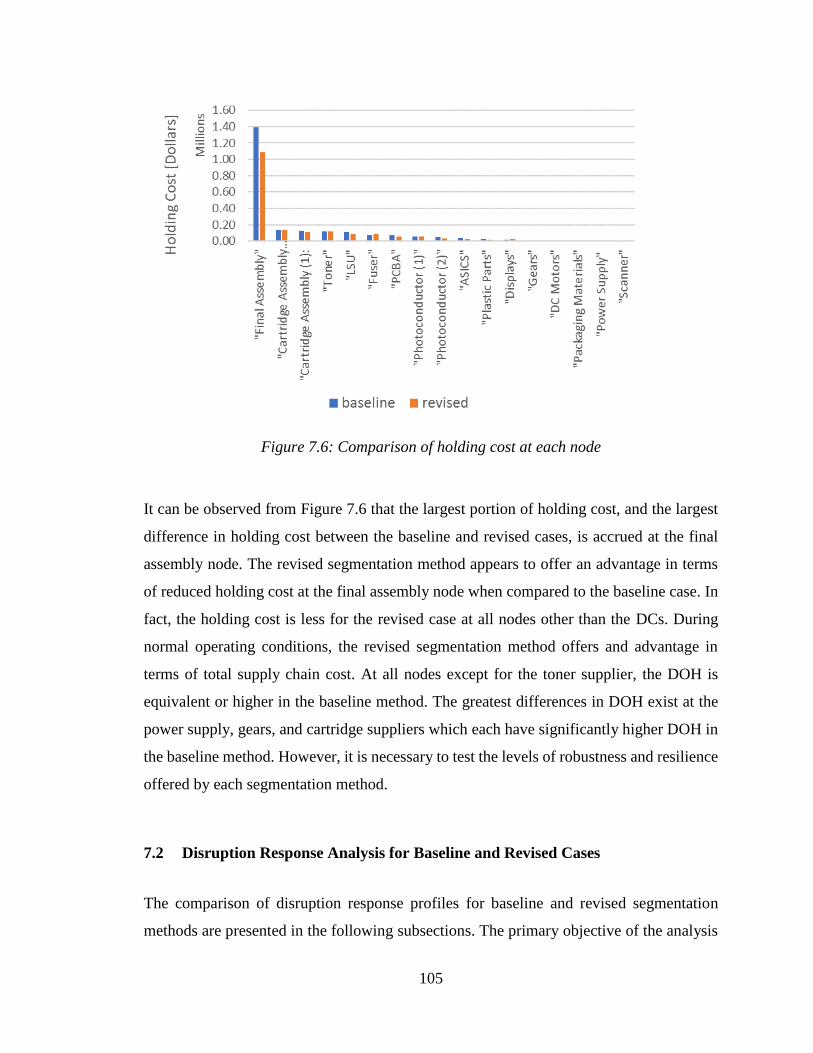
105
Figure 7.6: Comparison of holding cost at each node
It can be observed from Figure 7.6 that the largest portion of holding cost, and the largest
difference in holding cost between the baseline and revised cases, is accrued at the final
assembly node. The revised segmentation method appears to offer an advantage in terms
of reduced holding cost at the final assembly node when compared to the baseline case. In
fact, the holding cost is less for the revised case at all nodes other than the DCs. During
normal operating conditions, the revised segmentation method offers and advantage in
terms of total supply chain cost. At all nodes except for the toner supplier, the DOH is
equivalent or higher in the baseline method. The greatest differences in DOH exist at the
power supply, gears, and cartridge suppliers which each have significantly higher DOH in
the baseline method. However, it is necessary to test the levels of robustness and resilience
offered by each segmentation method.
7.2 Disruption Response Analysis for Baseline and Revised Cases
The comparison of disruption response profiles for baseline and revised segmentation
methods are presented in the following subsections. The primary objective of the analysis

106
is to demonstrate how the inventory of both finished goods and incoming raw material is
affected by the loss of capacity at the disrupted node. The detailed response data is studied
for a disruption that begins at simulated hour 720, midway through the second quarter of
the simulated runtime. During the disruption, full loss of production capacity is
experienced by the disrupted node. After a duration of 480 hours, or sixty 8-hour “work
days”, the production capacity of the affected node begins to ramp back up to its normal
level. An assumption is made that the disruption duration is the same for all scenarios.
Realistically speaking, the disruption duration would not be known at its moment of
occurrence and would vary by supplier due to response capability. The duration is held
constant in the proposed scenarios to simplify interpretation of the results. The study is
repeated with four points of disruption origin: cartridge assembly, toner, power supply, and
PCBA suppliers. To study the effect of the disruption’s start time and severity, the
experiments are repeated using combinations where the disruption begins at hour 1680,
midway through quarter four, and with 50% loss of capacity. The full list of scenarios is
summarized in Table 7.1. The full table is conducted for both baseline and revised
segmentation methods.
Table 7.1: Summary of disruption scenarios
Scenario Dis. Origin Start Time Severity
1 CAR Dis1 Q2 0%
2 CAR Dis2 Q4 0%
3 CAR Dis3 Q2 50%
4 CAR Dis4 Q4 50%
5 TON Dis1 Q2 0%
6 TON Dis2 Q4 0%
7 TON Dis3 Q2 50%
8 TON Dis4 Q4 50%
9 POW Dis1 Q2 0%
10 POW Dis2 Q4 0%
11 POW Dis3 Q2 50%
12 POW Dis4 Q4 50%
13 PCBA Dis1 Q2 0%
14 PCBA Dis2 Q4 0%
15 PCBA Dis3 Q2 50%
16 PCBA Dis4 Q4 50%

107
In sections 7.2.1 – 7.2.4 the results form scenarios 1, 5, 9, and 13 are studied in detail to
demonstrate the propagation in impact in inventory levels from disruption origin to the
DCs. The results from the remaining scenarios are summarized in section 7.3.
7.2.1 Disruption at Cartridge Supplier
Scenario 1: Baseline Segmentation Method
The first disruption scenario assessed occurs at cartridge supplier location 1. Information
regarding the section of the supply chain directly connected to the disrupted node is
summarized in Figure 7.7. The use of single or dual sourcing strategy for each component
is indicated by the number of houses, and the facility that will be affected by the disruption
is shown with red fill color. In the baseline case, management is using a single-source
strategy for cartridge assembly. However, cartridge assembly also occurs in two separate
geographic locations. Production facilities shown inside the same green box exist in the
same geographic location.
Figure 7.7: Partial SC map showing disruption at cartridge supplier location 1
(Baseline)

108
The transportation delay required between geographic locations (in terms of number of
ticks in the simulation model) is indicated by the number along the link between boxes. If
the suppliers for a given component have visibility into the buyer’s production rate, a small
eye is shown in the bottom left corner of the box. If there is no visibility, a red ‘x’ is shown
next to the eye. Finally, the desired on-hand (DOH) inventory at each supplier is indicated
in the bottom right of each box in terms of the number of hours of production. The values
for DOH apply to each facility. If the number shown is eight hours for a dual-sourced
product, then both the primary and dual aim to keep eight hours of inventory. Although
each supplier may or may not be able to maintain its DOH, this number provides an
indication of which nodes have goals of maintaining a larger or smaller inventory buffer.
The cartridge supplier has a direct connection to the DCs. It supplies aftermarket cartridges
directly to the DC’s. These aftermarket cartridges are sold separately from the printer and
have a separate demand. The cartridge supplier is also a 1st tier supplier to final assembly
(FIN). Each printer that is assembled at FIN must be equipped with a printer cartridge. The
disruption affects the supply chain’s ability to meet demand for both the aftermarket
cartridge and the printer itself, since the printer cannot be shipped without a cartridge.
The cartridge inventory response to the disruption at cartridge supplier location 1 is shown
in Figure 7.8. Enlarged versions of the plots within Figure 7.8 can be found in Appendix
C.
Each plot is based on data from thirty simulation replications. Inventory data is output at
each tick in the simulation, so the plotted result is the average of thirty data points for each
time step. For clarity, the upper and lower half-widths are excluded from the plots.

109
Figure 7.8: Inventory response to disruption at cartridge supplier location 1 (Baseline)

110
The immediate response to the disruption is seen in the plot of cartridge inventory at
cartridge supplier location 1. Since the cartridge supplier loses its capacity, its inventory is
depleted to zero soon after the disruption start at hour 720 (see Appendix C for larger chart).
Although the option is present, no alternate supplier engages during the disruption or
recovery periods. The signal to open the alternate is triggered, but the alternate startup
delay is not reached before the disruption ends and orders shift back to the primary supplier.
At the final assembly node, the cartridge inventory is depleted and a significant amount of
backlog is accrued. The figure showing the cartridge inventory at the DCs is the average
inventory over the six DCs. Upon closer examination, it is determined that the backlog
only occurs at DCs 1-3, while normal inventory levels are maintained at DCs 4-6. This
behavior is logical as the disrupted cartridge supplier is connected to DCs 1-3, and DCs 4-
6 are supplied by the unaffected cartridge supplier location. The response gives an
indication that when the backlog does arise, the information is not being effectively
communicated to the final assembly node, so it is not delivering cartridges to reduce the
backlog, even when it has some availability in supply.
The response of total supply chain cost to the disruption at the cartridge supplier is shown
in Figure 7.9. It can be clearly noted that the supply chain cost increases above the normal
operating bound around the time of the disruption. This increase may be due in part to the
increase in material cost during the disruption period. During the disruption, the material
cost increases by 50%, but this effect is soon balanced out as the amount of available
inventory is depleted.

111
Figure 7.9: Total SC cost (Baseline)
Scenario 1: Revised Segmentation Method
Strategic changes resulting from use of the revised segmentation method are shown in
Figure 7.10. Changes include dual sourcing at the cartridge supplier and removal of
visibility at the cartridge and gear suppliers. Also, the overall DOH at all the cartridge
supplier locations is reduced from the baseline method.

112
Figure 7.10: Partial SC map showing disruption at cartridge supplier location 1
(Revised)
The supply chain’s disruption response profile when the revised segmentation method is
used, shown in Figure 7.11, can be starkly contrasted to the response of the baseline case.

113
Figure 7.11: Inventory response to disruption at cartridge supplier location 1 (Revised)

114
The effect of removed visibility at the cartridge suppliers can be seen in cartridge inventory
at the DCs. As it was observed in the non-disruption analysis, the cartridge inventory at
DCs shows a marked decrease during quarters four and eight, in alignment with the periods
of increased demand. The decrease in cartridge inventory during the second quarter is due
to the disruption at cartridge supplier location 1. An increase in cartridge buffer inventory
at the DCs prevents the accumulation of the magnitude of backlog seen in the baseline case.
This result is an early indication that buffer inventory held at the DCs is more effective at
reducing disruption impact than inventory held further back in the supply chain.
The behavior of supply chain cost, shown in Figure 7.12, does not appear to be significantly
affected by the occurrence of the disruption. A decrease in the cost is observed in quarters
four and eight, corresponding to the depletion of inventory due to higher demand. A brief
increase in cost is observable in quarter two, but the levels are never in excess of the upper
bound determined during the non-disruption case.
Figure 7.12: Total supply chain cost (Revised)

115
7.2.2 Disruption at Toner Supplier
Scenario 5: Baseline Segmentation Method
The disruption scenarios originating at the toner supplier are subject to the same network
structure and strategic options as previously indicated in Figure 7.7 and Figure 7.10.
However, the disruption originates at the tier 2 supplier. Figure 7.13 demonstrates how the
interruption of toner supply propagates from the toner supplier to the cartridge supplier
locations, and ultimately affects delivery of cartridges to the DCs.

116
Figure 7.13: Inventory response to disruption at toner supplier (Baseline)

117
The toner supply is segmented as a strategic supplier for both the baseline and revised
segmentation methods. Toner is single sourced due to its strategic nature and has the
potential to disrupt both cartridge supplier locations. From Figure 7.13, it is seen that the
disruption in toner supply is immediately passed on to the cartridge suppliers and the
inventory does not fully recover until mid-way through the second year. The alternate
startup delay at the toner supplier is much longer than the disruption duration of 480 hours,
and so the alternate supplier is no able to engage and reduce the impact. The cartridge
inventory at the DCs is thus subject to a long disruption with significant backlog
accumulation. Although now shown in Figure 7.13, a similar response is observed in the
final assembly inventory at the DCs because each final assembly must be equipped with at
cartridge.
The total supply chain cost response is shown in Figure 7.14. The cost decrease seen results
from the depletion of both final assembly and cartridge inventory at both DCs and the final
assembly node. Although the response indicates a reduction in cost, it should be noted that
the calculation of cost does not account for any penalty for late delivery. The response
should therefore not be misconstrued as an indication of a cost advantage during the
disruption recovery.
Figure 7.14: Total SC cost with disruption at toner supplier (Baseline)

118
Scenario 5: Revised Segmentation Method
The toner supplier is segmented in the strategic category when both the baseline and
revised methods are used. For this reason, a substantial change in the inventory and cost
response is not expected. However, the cartridge suppliers are directly connected between
the toner supplier and the DCs, and the strategic changes for the cartridge suppliers still
apply and may have an effect although they are not at the origin of the disruption. The toner
and cartridge inventory response is summarized in Figure 7.15. Upon closer examination
of the result, the difference in strategy at the cartridge suppliers appears to have minimal
effect. There are no major differences in the disruption response between baseline and
revised methods. Total supply chain with the disruption at the toner supplier is shown in
Figure 7.16. These results are indicative of the potential vulnerability associated with a
strategic supplier.

119
Figure 7.15: Inventory response to disruption at toner supplier (Revised)

120
Figure 7.16: Total SC cost with disruption at toner supplier (Revised)
7.2.3 Disruption at Power Supply Supplier
Scenario 9: Baseline Segmentation Method
Power supply is a tier 1 supplier to final assembly. The portion of the printer supply chain
linking power supply to the DCs is depicted in Figure 7.17. In the baseline case, power
supply is segmented as a bottleneck supplier. A single sourcing strategy is used, with
visibility and a higher level of DOH.
Figure 7.17:Partial SC map showing disruption at power supply supplier (Baseline)

121
Figure 7.18 presents the power supply inventory at the power supply supplier and final
assembly. Also depicted are the final assembly inventory at final assembly and at the
DCs.

122
Figure 7.18: Inventory response to disruption at power supply supplier (Baseline)

123
The power supply and final assembly inventory is quickly depleted after the disruption
begins at the power supply supplier. Despite a seemingly quick recovery after the
disruption ends at tick 1200, the effects of limited final assembly inventory at the DCs
extend well beyond the end of the disruption, with normal levels not achieved again until
around tick 2600. By contrast, inventory levels at the power supply supplier and final
assembly are largely recovered by tick 1500. The peak of final assembly backlog does
occur around tick 1500, but due in part to the capacity limitations of final assembly, it takes
substantial time to eliminate the backlog at each DC. As shown in Figure 7.19, the extended
time-to-recovery also applies to the total supply chain cost.
Figure 7.19: Total supply chain cost with disruption at power supply (Baseline)
Scenario 9: Revised Segmentation Method
When the revised segmentation method is employed, the power supply suppliers falls into
the non-critical category. Implications of the change in segment include removal of
visibility, addition of dual sourcing, and reduction in the DOH at each facility. The
section of the supply chain as described is shown in Figure 7.20.

124
Figure 7.20: Partial SC map showing disruption at power supply supplier (Revised)
The inventory response for the supply chain segmented by the revised method is
summarized in Figure 7.21. The adjustment in strategy has significant improvement both
resilience and robustness.

125
Figure 7.21: Inventory response to disruption at power supply supplier (Revised)

126
In fact, the disruption at the power supply location does not have any significant impact on
the inventory of final assembly at the DCs. The dual supplier at the power supply location
is sufficiently capable of handling the orders when the primary supplier fails. As a result,
there is no noticeable change in the inventory levels at final assembly when compared to
the no-disruption scenario. It is also shown, in Figure 7.22, that the improved disruption
recovery is achieved without any significant change from the normal operating cost levels.
The result indicates a possible advantage to using dual sourcing with lower DOH as
compared to single sourcing with higher DOH.
Figure 7.22: Total SC cost with disruption at power supply supplier (Revised)
7.2.4 Disruption at PCBA Supplier
Scenario 13: Baseline Segmentation Method
The PCBA supplier falls into the leverage category with both baseline and revised
segmentation methods. The portion of the supply chain most closely linked to the PCBA
supplier is shown in Figure 7.23. Strategic options for PCBA include the use of dual-
sourcing, no visibility, and a lower DOH level. It is also relevant to note that PCBA is a

127
relatively highly-connected node, acting as a middle tier between displays, ASCIS, and
final assembly.
Figure 7.23: Partial SC map showing disruption at PCBA supplier (Baseline)
Figure 7.24 summarizes the response of PCBA and final assembly inventory to a
disruption at the PCBA supplier.

128
Figure 7.24: Inventory response to disruption at PCBA supplier (Baseline)

129
The effects of the disruption are seen at the final assembly node during the second quarter.
During quarters four and eight the inventory levels drop in association with the periods of
increased demand. The dual source for PCBA continues to deliver products to final
assembly throughout the disruption, and the alternate supplier becomes active for a brief
period as the primary supplier is ramping its capacity back to normal operating levels. The
PCBA disruption does not appear to have a substantial impact on the inventory of final
assemblies at the DCs. The supply chain cost, shown in Figure 7.25, diminishes during
quarters four and eight during which the inventory levels are reduced because of high
demand.
Figure 7.25: Total SC cost with disruption at PCBA supplier (Baseline)
Scenario 13: Revised Segmentation Method
There is no change in the strategic choices within the portion of the supply chain directly
linked to PCBA inventory when the revised segmentation method is applied. Therefore,
Figure 7.23 is still a good representation for effective strategies in the pertinent disruption
scenario and need not be repeated. As demonstrated in Figure 7.26, the supply chain’s
resilience and robustness are reduced when the revised segmentation method is applied.

130
Figure 7.26: Inventory response to disruption at PCBA supplier (Revised)

131
Because there is no change in the strategies at the PCBA supplier itself, the increase in
severity of impact must be due to the behavior of the surrounding suppliers. The response
in PCBA inventory at the PCBA supplier itself follows nearly the same pattern in both
baseline and revised cases. The distinction in the response of the two scenarios is most
evident at the final assembly and DCs. The inventory response was observed at the displays
and ASICS suppliers, which supply the PCBA node with raw material. It is discernable
that after the PCBA disruption, the raw material inventory of displays at the PCBA node
is not able to recover its normal operating levels. Without the displays, the PCBA supplier
cannot complete production at the required rate to fully supply the final assembly
operation. The inability of the PCBA supplier to recover its raw material of displays can
be attributable to a combination of low DOH and a lack of visibility at the displays supplier.
After the disruption, the final assembly production continues until its supply of PCBAs is
exhausted. During recovery, the PCBA supplier must increase its production rate to
replenish the lost inventory as well as satisfy new demand. Without visibility, the displays
node does not update its DOH or its production rate. If the DOH at the displays supplier
were sufficiently high, it would still be able to resupply the PCBA node. However, in the
revised case, production capacity and by association, DOH, are set at lower levels than
during the baseline case. The higher DOH and production capacity at displays explains its
ability to withstand the effects of the disruption despite its lack of visibility.
Total supply chain cost response to the PCBA disruption reflects the inventory pattern and
is shown in Figure 7.27.

132
Figure 7.27: Total SC cost with disruption at PCBA supplier (Revised)
7.3 Effects of Demand Seasonality and Disruption Severity
The disruption scenarios are repeated with start time either in quarter 2 (Q2) or quarter 4
(Q4) to determine the effects of demand seasonality on robustness and resilience. Q2 is a
period of typical demand whereas the demand in Q4 is higher than other periods of the
year. For this reason, it is reasonable to expect a disruption that occurs in Q4, when
production rate is more likely to be close to its capacity, to have greater impact. It is also
possible to examine the effects of disruption severity on impact. In some disruption
scenarios, an incomplete loss of production capacity may occur. It is interesting to study
the effects that severity might have on the selection of the most resilient and robust
procurement strategies.
Figure 7.28 demonstrates how the resilience and robustness of the supply chain are affected
by the start time and severity of a disruption at the cartridge supplier. Robustness, as
measured by the maximum deviation from the lower bound appears to be better when the
disruption occurs in Q2. As expected, the complete loss of capacity results in a greater
maximum deviation from the lower bound, regardless of the disruption start time. It appears
that the supply chain may be more sensitive to disruption severity when the disruption
occurs in Q2. The supply chain resilience for the same disruption originating at the

133
cartridge supplier shows some unexpected behavior. The time-to-recovery decreases with
increased severity when the disruption starts in Q4, the period of higher demand.
Figure 7.28: Seasonality and severity effects with disruption at cartridge supplier
(Baseline)
As shown in Figure 7.29, the resilience and robustness show a different response to
disruption start time and severity when the revised segmentation method is used.
Figure 7.29: Seasonality and severity effects with disruption at cartridge supplier
(Revised)
The maximum deviation from inventory lower bound is sensitive to the disruption severity
only when the disruption starts in Q2. The time-to-recovery is longer when the disruption
begins in Q2, the period with lower demand. Looking back at the inventory response at the
DCs, the increased time-to-recovery can be explained by the high sensitivity of the
cartridge inventory to the periods of high demand. When the disruption occurs in Q2, the

134
cartridge inventory is reduced and makes the supply chain more susceptible to the high
demand in Q4. When the disruption occurs in Q4, both the disruption and the high demand
period coincide, isolating the disruptive effects.
The supply chain segmented with the baseline method appears to have similar resilience
and robustness to a disruption at the toner supplier, according to the result shown in Figure
7.30. The maximum deviation from lower bound and the time-to-recovery each increase
with disruption severity, as expected. Maximum deviation is slightly higher with the
disruption starts in Q2, but not to a significant degree.
Figure 7.30: Seasonality and severity effects with disruption at toner supplier (Baseline)
As seen in Figure 7.31, maximum deviation from the lower bound shows a similar
sensitivity to start time and severity in the revised segmentation case.
Figure 7.31: Seasonality and severity effects with disruption at toner supplier (Revised)

135
For the revised case the time-to-recovery does not show a sensitivity to the severity of the
disruption. The dependence of time-to-recovery on start time is more significant in the
revised segmentation case, with time-to-recovery being longer when the disruption occurs
in Q2. The supply chain is not able to fully recover from the impact of the disruption at the
toner supplier by the end of the simulation runtime. The time-to-recovery reflects the fact
that the disruption starting in Q2 occurs earlier and the supply chain spends a longer time
in the disrupted state.
Figure 7.32 summarizes the resilience and robustness of the supply chain to disruptions at
the power supply supplier. Unexpected patterns seen in the response include a reduction in
robustness as the disruption severity increases, and a higher resilience to disruptions
starting in Q4.
Figure 7.32: Seasonality and severity effects with disruption at power supply supplier
(Baseline)
The results shown in Figure 7.33, which indicate the resilience and robustness of the
supply chain segmented with the revised method, are provided for completeness.
However, only one of the four disruption scenarios originating at the power supply
caused a disruption in the final assembly inventory at the DCs. The supply chain shows
good robustness against this type of disruption when the revised segmentation strategies
were used.

136
Figure 7.33: Seasonality and severity effects with disruption at power supply supplier
(Revised)
The supply chain response to disruptions at the PCBA supplier are shown in Figure 7.34.
The resilience and robustness for the supply chain segmented with the baseline method
follow the expected trends. Robustness and resilience both decrease when 100% disruption
severity is realized and when the disruption occurs during the period of higher demand.
Figure 7.34: Seasonality and severity effects with disruption at PCBA supplier (Baseline)
When the revised segmentation method is used, the supply chain becomes for susceptible
to PCBA disruptions beginning during Q2. This effect is observed in Figure 7.35. Similar
to the disruption at the toner supplier, the supply chain in these scenarios cannot fully
recover due to an inability of the displays node to properly resupply the PCBA node with
raw material after the production recovers from the loss of capacity. The disruptions
starting at Q2 subject the supply chain to this effect for a longer period of time.

137
Figure 7.35: Seasonality and severity effects with disruption at PCBA supplier (Revised)
7.4 Baseline vs. Revised Comparison for all Scenarios
Some general observations can be made regarding the overall effectiveness of the baseline
and revised segmentation methods at guarding the supply chain against disruption impact.
First, for disruptions at the cartridge supplier, mixed results are seen depending on the
objective. As shown in Figure 7.36, the maximum deviation from lower bound is lower
when the revised segmentation method is used, while time-to-recovery is higher.
Figure 7.36: Resilience & robustness to disruption at cartridge supplier
A closer examination of the cartridge inventory response at the DCs reveals the supply
chain with the revised segmentation strategies provides better protection against the initial
disruption, but then due to the sensitivity to the high demand periods takes an extended
time to fully recover. The supply chain with the baseline strategies shows a more distinct

138
pattern of disruption and recovery, but allows the cartridge inventory levels to decrease
more drastically immediately after the disruption occurs.
As indicated in Figure 7.37, the effectiveness of the baseline and revised segmentation
methods is similar, but slightly favoring the baseline method when the disruption originates
at the toner supplier. Neither method, however, protects the supply chain well which
indicates the significance of a disruption occurring at a strategic supplier.
Figure 7.37:Resilience and robustness to disruption at toner supplier
The disruption impact for the scenarios starting at the power supplier show a clear
advantage to the revised segmentation method in Figure 7.38. As indicated by the
descriptions of section 7.2.3, the benefits are derived from the shift to a dual sourcing
strategy at the power supply supplier.
Figure 7.38: Resilience and robustness to disruption at power supply supplier
The disruption at the PCBA supplier, on the other hand, is better-handled by the baseline
case as indicated in Figure 7.39.

139
Figure 7.39: Resilience and robustness to disruption at PCBA supplier
The reduction in resilience and robustness observed when the revised segmentation method
is used is attributable to a lack of visibility at the displays supplier, which provides raw
material to the PCBA supplier, combined with an insufficient DOH at the displays supplier.
It is interesting to note that the problem in this case does not originate at the supplier that
was directly affected by the disruption. Rather, the after-effect and lack of preparation and
communication between the affected node and its supplier is the source of vulnerability.
This observation highlights the importance of considering the possible impacts of a
disruption throughout the entire supply chain rather than only at the first-tier suppliers.

140
8 Discussion
Through examination of the simulation results, general conclusions can be drawn about
how to select the best segment for a given supplier and possibilities for future improvement
of segmentation methods. First, the observed results are examined with respect to the initial
hypotheses a – d.
a) The revised segmentation method will increase resilience of the supply chain
compared to baseline method.
Disruption impact assessment of the different scenarios indicates mixed results regarding
the effectiveness of the two segmentation methods at increasing resilience and robustness.
Better disruption response at the DCs is observed in the scenarios with disruption
originating at the power supply and cartridge suppliers. For the cartridge disruption, a more
contained period of disruption and recovery is observed with the baseline method than the
revised method, as seen in Figure 7.8 and Figure 7.11. However, the backlog that compiles
in the baseline case is much greater than in the revised case, so the revised case is judged
as offering the preferable response. On the other hand, for the disruption scenarios
originating at the toner and PCBA suppliers, the baseline segmentation method appears to
offer superior resilience and robustness. The resilience and robustness observed in the
inventory at the DCs is a result of the strategies of all suppliers in the supply chain.
Therefore, it is difficult to explain the behavior as a result of a change in segmentation of
any one node. However, some general observations are made.
The analysis of the cartridge disruption scenarios provides an indication that maintaining
buffer inventory at the DCs increases robustness better than maintaining buffer at the final
assembly node and farther up the supply chain. The buffer at the DCs is more capable of
meeting the new demand that arises during the disruption period. Keeping inventory at the
final assembly node increases cost significantly because of the number of types of raw
material and the value of the finished goods. At the suppliers, the DOH is designed to last
no more than around 24 hours. It is not cost-feasible to maintain enough finished goods
inventory at a supplier to last throughout the duration of significant disruption.

141
Strategies of dual sourcing and visibility appear to be more important to increasing
resilience and robustness. From analysis of disruptions at the power supply, there seems to
be a clear advantage to the dual source strategy as opposed to the single source strategy
with higher buffer inventory. This observation may be predicated on a requirement that the
dual supplier has sufficient capacity so that it can ramp up its production during the period
in which the primary supplier is not producing.
Observations from the disruption response at the PCBA supplier indicate that the disrupted
supplier’s suppliers, namely the displays supplier, needs visibility to know how and when
to send more material for replenishment of depleted inventory once the disrupted
production capacity is regained. Lacking visibility, it is necessary for the lower tier supplier
to have a combination of enough capacity and high enough DOH so that it can replenish
material with an increased demand, despite the fact it does not see the problem.
Although the baseline and revised segmentation methods show mixed results, it can
generally be concluded that strategies of dual sourcing & visibility are most effective at
increasing resilience and robustness. Increased DOH, and the extra capacity associated
with it, is more important for nodes near the disruption. As the suppliers to the disrupted
node experience a demand surge during and after disruption recovery, sufficient DOH and
capacity are important for rapid replenishment of the disrupted node. In the printer supply
chain case study, the revised method shifted suppliers toward the leverage and non-critical
segments. As per the general observations relating to strategy, the suppliers which could
be managed as leverage or non-critical generally showed increased resilience and
robustness.
It is interesting to note the cause for the cartridge, power supply, and gears suppliers shift
to the left-hand side of the segmentation matrix. First, each of these suppliers scored low
on the additional resilience-oriented variables used in the revised segmentation method.
The suppliers had fast to moderate ramp up time and low variability in transportation time.
In addition, each of these suppliers was near the cutoff point between high and low ranking
for market complexity based on the baseline segmentation variables. Other suppliers
showed greater increase in market complexity due to the additional resilience-oriented
variables. Ramp-up time and logistics variability relate to a supplier’s ability to open a new

142
location quickly and switch efficiently between sourcing locations. Suppliers without
switching and ramp up capability are less effectively managed with dual source strategy
and may show greater vulnerability to disruption.
b) A disruption at a strategic supplier is likely to have a more severe impact on the supply
chain than a disruption at a non-critical supplier. The impact after a disruption at
bottleneck or leverage suppliers is likely to fall into a middle range of severity.
The disruption at the toner supplier demonstrates the potential significance of a disruption
at a strategic supplier. Both strategic and bottleneck nodes are shown to be vulnerable to
disruption primarily because they do not employ dual sourcing, which is because of higher
market complexity and limited supplier availability for the components. Strategic nodes
appear to be most vulnerable because they also maintain lower DOH and generally are used
for suppliers of higher cost components. A company tends to become dedicated to its
strategic suppliers in business, which can be a point of strength but also a source of
vulnerability as it may be difficult to find an alternate supply source. If a strategic supplier
relationship is desired, it might be worthwhile to consider having a highly responsive
alternate supplier with minimal startup delay. Contrary to the hypothesis, the results
indicate that disruptions at strategic and bottleneck suppliers would both have a tendency
toward more severe impact to disruptions. Leverage and non-critical suppliers would tend
to suffer from less severe impact.
c) Disruptions that start during a period of high demand are likely to have a stronger
impact than those that occur during normal demand periods.
As shown in section 7.3, disruptions which begin in periods of higher demand, namely
during the fourth quarter of the simulated runtime, tend to cause greater disruption impact.
Exceptions include observations for the cartridge disruption with revised segmentation and
toner disruption with revised segmentation. The influence of the demand pattern is highly
dependent on the amount of inventory buffer at the DCs. In the revised case, the cartridge
buffer is reduced and therefore the demand increase and disruption have a combined effect.
Offsetting the disruption and period of increased demand only has the effect of elongating
the period of disruption. There is a general indication from this result that having a larger
finished goods buffer at the DCs can protect against the combined effects of demand

143
escalation and disruption. Therefore, it would be logical in future planning to increase the
finished goods inventory during the periods of expected high demand.
d) Disruptions that cause a greater reduction in production capacity will have a greater
impact on the supply chain.
The results indicate mixed response to changes in disruption severity from 50% loss of
capacity to 100% loss. In several cases, the robustness or resilience show no sensitivity to
the disruption severity. For the baseline segmentation case with cartridge disruption
starting in Q4 the time-to-recovery was negatively associated with disruption severity. One
possible explanation for the mixed result is that although only 50% of the production
capacity was lost, the disruption increased demand during Q4 prevented the remaining
capacity from keeping up with the desired production rate. In general, the effects of the
segmentation method and the seasonal demand appear to outweigh the effects of disruption
severity.
In addition to the observations on resilience and robustness, some general conclusions can
be drawn with respect to the normal operating cost resulting from each segmentation
method. Higher inventory and higher visibility strategies tend to result in a higher normal
operating cost. As noted in section 7.1 the cost is dominated by holding cost, and holding
cost is largely determined by DOH. Strategies of higher DOH level are associated with the
bottleneck segment. Visibility can also increase cost because a supplier with visibility may
increase its production rate to match the expected demand of its buyer. In so doing, the
supplier can exceed its DOH, while this would not happen at a supplier with no visibility.
Therefore, from a cost perspective it makes sense to segment most suppliers as leverage or
non-critical if it is feasible to do so. Feasibility of segmenting as leverage or non-critical
largely relates to the availability of a dual source, and the length and variability of
transportation delay from the dual source. In the printer case study, the revised
segmentation method showed a stronger tendency to segment suppliers into the lower cost
segments, and in general the cost of the revised supply chain was reduced. It then would
be appropriate to use strategic or bottleneck strategies when there is no dual source
available, or a dual source is available but is far away with variable transportation delay,
or otherwise unreliable delivery. Availability of suppliers and transportation delay and

144
reliability should weigh in highly when assessing market complexity, which essentially
differentiates the dual and single-source suppliers.
Results indicate an advantage to segmenting most suppliers as leverage or non-critical with
respect to normal operating cost, resilience, and robustness. However, in cases of high
market complexity it is not always possible to use these strategies. The inability to use a
dual sourcing method largely determines if a supplier should be moved to bottleneck or
strategic segments. When deciding between bottleneck and strategic segments, the cost of
the component is a primary consideration, along with the connectedness of the supplier and
component criticality. Criticality can refer to the importance of the component to the
customer’s purchase decision, and the potential for design innovations relating to that
component. Due to limitations in the simulation model, not all factors of purchasing
importance could be considered, but opportunity exists for further extension and study of
different indicators for using bottleneck vs. strategic segments.
This research presents an argument that the portfolio segmentation methods similar to the
approach presented by Kraljic (1983) are limited by their focus on operational risk and
general goal of selecting the best strategies for normal operating conditions. Realistically,
the established strategies for buyer-supplier interaction also affect disruption response
capability. The results from the presented case study and ABMS indicate that the choice of
dual or single sourcing, whether to establish buyer-supplier visibility in production
planning, and the DOH at nodes near a disruption each have a significant effect on the
supply chain resilience and robustness. Post-disruption recovery strategies should be
developed and are important to mitigate the disruption impact, but the results of this
research indicate that the effectiveness of these recovery actions depends on the state of
disruption preparedness provided by day-to-day procurement strategy. The revised
segmentation method demonstrated mixed capability for improving the resilience and
robustness of the supply chain. There is a need to further-examine the connection between
the individual segmentation variables and their implications on choice of procurement
strategy.

145
9 Summary and Future Work
From the research perspective, this work contributes an organized set of factors that should
be considered in a supplier segmentation method oriented toward the enhancement of
resilience and robustness. Furthermore, a revised segmentation method was specified
which incorporated a subset of resilience-oriented factors. The incorporation of the
resilience-oriented factors had the general effect of creating a greater distinction between
suppliers with higher and lower potential for disruption impact. An agent-based model and
simulation was developed to study the impact of different disruption scenarios on the
supply chain as segmented with the revised segmentation method.
The revised segmentation method was compared to a baseline method based on an
assessment of suppliers during normal conditions. The two segmentation methods were
compared in the context of a laser printer supply chain. Practical results from the research
include general observations from the disruption scenarios. It was indicated that the
procurement strategies associated with the leverage and non-critical segments were
advantageous from both the normal operating cost and disruption response perspective.
However, these strategies are not always feasible in which case strategic or bottleneck
strategies should be employed.
Opportunities exist for further study and improvement of the segmentation method. The
importance of the alternate supplier should be studied in greater detail. Decision processes
relating to how and when the alternate supplier is signaled to open should be incorporated
in the simulation. The costs and time delays relating to the opening and ramp up of an
alternate supplier have potential to greatly affect the practicality of using a single-sourcing
method. Additional resilience-enabling factors could be considered in the segmentation
process as the decision models associated with the new factors are included in the
simulation. Given the availability of supplier data, it would be worthwhile to consider using
clustering techniques or principal component analysis to go beyond the original portfolio
segmentation approach. The revised portfolio segmentation methods employed rely on a
relative ranking of suppliers. It would be worthwhile to seek out fixed cutoff points for the
two segmentation dimensions. For example, it could be determined if there is a fixed

146
amount of market complexity for which dual or single sourcing strategy is more effective
from the operational and disruption response perspectives.
The complexity of the decision processes modeled in the ABMS was controlled to simplify
interpretation of results. The supplier behavior was differentiated enough to test the
hypothesis regarding the effects of strategy associated with different supplier segments.
There is opportunity to extend the ABMS capabilities to better-reflect the intricacies of
decision making processes.
A limitation in the work is that disruptions are assumed to have the same length, regardless
of the supplier or the associated disruption source. Eliminating this assumption, the
duration of the disruption would be dependent on internal supplier capabilities. In future
work, the connection between supplier characteristics and ability to regain capacity after
disruption could be explored in greater detail.
In addition, customer behavior patterns could be explored. The customer response to
stockouts at the DCs may vary depending on the type of customer. In some cases, the
customer may be very loyal and willing to wait for inventory to become available. The
company may attempt to retain customers by absorbing a late fee. These factors affect the
cost response due to disruption and may be interesting to explore in future simulation
models. The ABMS modeling paradigm lends itself well to the study of supplier
relationship behaviors. For example, supplier characteristics can be included in the model
that specify whether a supplier would favor the focal company or possibly another of its
customers.
This research assumes that capacity at the supplier is dedicated to the printer supply chain
for the focal company. In some instances, a supplier may share its production capacity
across multiple customers. These considerations can be explored with future developments
of the supply chain ABMS. Finally, it is worthwhile to consider modifying the supply chain
ABMS to improve flexibility, so that it can be more easily applied to different supply chain
networks. The improved flexibility for multiple applications would allow repeated studies
of different segmentation methods so that their effectiveness could be demonstrated in
different contexts.
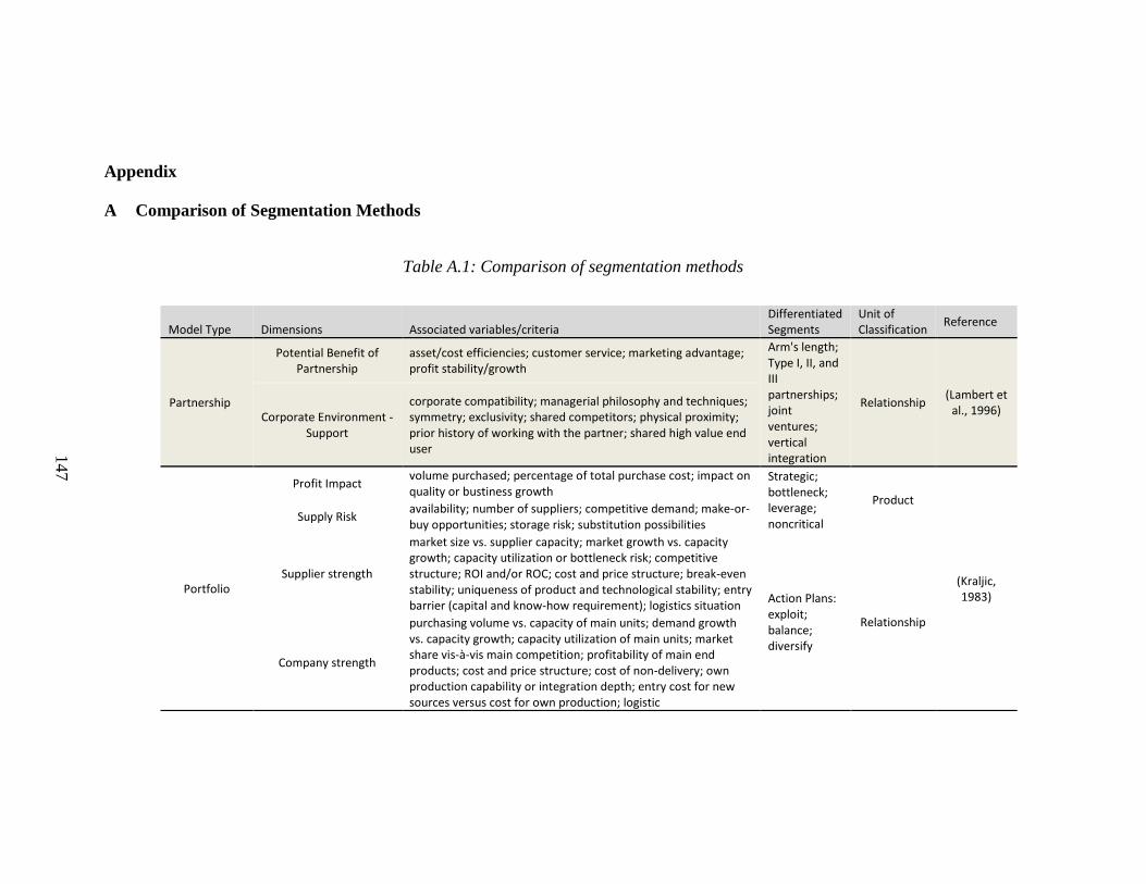
147
Appendix
A Comparison of Segmentation Methods
Table A.1: Comparison of segmentation methods
Model Type Dimensions Associated variables/criteria Differentiated Segments
Unit of Classification
Reference
Partnership
Potential Benefit of Partnership
asset/cost efficiencies; customer service; marketing advantage; profit stability/growth
Arm's length; Type I, II, and III partnerships; joint ventures; vertical integration
Relationship (Lambert et
al., 1996) Corporate Environment -
Support
corporate compatibility; managerial philosophy and techniques; symmetry; exclusivity; shared competitors; physical proximity; prior history of working with the partner; shared high value end user
Portfolio
Profit Impact volume purchased; percentage of total purchase cost; impact on quality or bustiness growth
Strategic; bottleneck; leverage; noncritical
Product
(Kraljic, 1983)
Supply Risk availability; number of suppliers; competitive demand; make-or-buy opportunities; storage risk; substitution possibilities
Supplier strength
market size vs. supplier capacity; market growth vs. capacity growth; capacity utilization or bottleneck risk; competitive structure; ROI and/or ROC; cost and price structure; break-even stability; uniqueness of product and technological stability; entry barrier (capital and know-how requirement); logistics situation
Action Plans: exploit; balance; diversify
Relationship
Company strength
purchasing volume vs. capacity of main units; demand growth vs. capacity growth; capacity utilization of main units; market share vis-à-vis main competition; profitability of main end products; cost and price structure; cost of non-delivery; own production capability or integration depth; entry cost for new sources versus cost for own production; logistic

148
Table A.1 continued
Model Type Dimensions Associated variables/criteria Differentiated Segments Unit of Classification
Reference
Involvement
Nature of Products interface complexity; rate of technological change; end consumer perception influence
Critical systems (high cost, OEM provides supplier with performance specifications); hidden components (low cost simple components defined by physical specifications); invisible subassemblies (moderate cost, suppliers are provided with performance specification and detailed physical dimensions); simple differentiators (moderate cost simple assemblies; suppliers are provided with detailed physical specifications)
Product
(Laseter and Ramdas, 2002)
Cost Structures unit product cost; amortized development cost; manufacturing scale
Nature of OEM-Supplier Interaction type of specifications passed to the supplier
Portfolio Product Complexity
technicality of product; need for user input in making a sound purchase; importance of tight product specifications; criticality of product performance with high differentiation between various suppliers' products
close relationships; strategic partnerships; simple contracts; global trading
Relationship (Hadeler and Evans, 1994)
Product Value Potential
dollar volume; potential for significant price reduction; potential for getting significant value-added benefits from suppliers; risk to profit or safety in case of supply shortage or quality problems
Partnership
Collaboration
26 variables from NIST 'Quickview' manufacturing survey; 5 most influential: early supplier involvement in product development; strategic vision; customer/material supplier certification; insufficient employee training; equipment supplier certification
commodity supplier; collaboration specialist; technology specialist; problem-solving supplier
Supplier (Kaufman et
al., 2000)
Technology
22 variables from NIST 'Quickview' manufacturing survey; 5 most influential: expert machine utilization; quality function deployment; process manufacturing know-how; inexpert machine utilization; advanced process technology management

149
Table A.1 continued
Model Type Dimensions Associated variables/criteria Differentiated Segments Unit of Classification
Reference
Portfolio
Strategic Importance of the Purchase competence (of buyer), economic, and image factors
bottleneck; strategic; non-critical; leverage
Product
(Olsen and Ellram, 1997)
Difficulty of Managing the Purchase Situation
product, supply market, and environmental characteristics
Relative supplier attractiveness
financial and economic, performance, technological, organizational/cultural/strategic, flexibility to environmental changes, and safety factors
action plans: strengthen supplier relationship; improve supplier attractiveness or relationship performance; reduce resources allocated to the relationship
Relationship
Strength of Relationship
economic factors, character of the exchange relationship, cooperation between buyer and supplier, distance between buyer and supplier
Portfolio
Buyer's Specific Investments
tangible: buildings, tooling, equipment; intangible: people, time, knowledge
captive buyer; strategic partnership; market exchange; captive supplier
Relationship (Bensaou,
1999) Supplier's Specific Investments
tangible: plant location/layout, specialized facilities/dies; intangible: guest engineers, information system development
Portfolio
Buyer Dependency Risk
value added to the customer; irreplaceability of the supplier
non-strategic; strategic; asymmetric Relationship (Hallikas et al., 2005) Supplier Dependency
Risk value added to the supplier; irreplaceability of the customer
Portfolio
Willingness to Maintain Relationship
21 variables identified described by quadrant, not otherwise characterized
Supplier (specific
functions)
(Rezaei and Ortt, 2012)
Performance Capability
46 variables identified
Involvement Strategic Nature of Inputs
necessary but non-strategic; strategic durable arm's-length relationship; strategic partnerships
Supplier (Dyer et al., 1998)

150
B Resilience-Enabling Factors Literature Review Summary Tables
Table B. 1: Elements of visibility and data analysis
Reference
Extent or timeliness of information collection and/or exchange
Uncertainty in the shared information
Ability to convert information into useful knowledge
Types of information collected and/or shared
Use of tools, methods, and procedures
(Blackhurst, Craighead et al. 2005)
real-time information sharing
correctness of shared information
predictive analysis to foresee problems
dynamic risk indices at each node
(Brandon-Jones, Squire et al. 2014)
sharing inventory and demand levels
Information Technology and support technology
(Basole and Bellamy 2014) visualization tools
(Craighead, Blackhurst et al. 2007)
dissemination of pertinent disruption information
detection of pending or realized disruptions
(Pettit, Croxton et al. 2013)
business intelligence gathering
information exchange knowledge of status of product, equipment, and people Information Technology
(Shao 2013)
information accessibility
frequency of information sharing
real-time information sharing/timely sharing of supply information
correctness of shared information
knowledge on status of material flow
(Jüttner and Maklan 2011)
event monitoring (environment)
event monitoring (internal to the supply chain)
knowledge on status of material flow
(Sheffi and Rice Jr 2005)
Statistical Process Control/anomaly detection
shipment visibility systems/RFID

151
Table B. 1Table B. 1: Elements of visibility and data analysis continued
Reference
Extent or timeliness of information collection and/or exchange
Uncertainty in the shared information
Ability to convert information into useful knowledge
Types of information collected and/or shared
Use of tools, methods, and procedures
(Ojha, Gianiodis et al. 2013)
awareness of optimal operating performance levels
(Hohenstein, Feisel et al. 2015) real-time monitoring early warning indicators
(Scholten, Scott et al. 2014)
event monitoring (internal to the supply chain)
knowledge on status of material flow
(Wieland and Wallenburg 2013)
screening and signaling
timeliness of sharing disruption data
knowledge of changes currently occurring
(Olcott and Oliver 2014) common knowledge base
integrated knowledge sharing routines/Information Technology infrastructure
(Ambulkar, Blackhurst et al. 2015)
awareness of pending disruptions
(Kleindorfer and Saad 2005)
use of compatible communication and information technologies
(Ponis and Koronis 2012)
knowledge management systems
(Ellis, Henry et al. 2010)
difficulty forecasting future developments due to technological uncertainty
volatility of standards for product price and quality performance

152
Table B. 2: Elements of Collaboration and Supplier Development
Reference
Mutual efforts: working towards a common objective
Decision Synchronization: shared use of information for mutual benefit
Supplier openness and efforts to meet buyer requirements
Presence of incentive alignment and risk sharing
Planning, organization and unification of employee efforts
Compatibility: cultural alignment
(Hohenstein, Feisel et al. 2015)
supplier development information sharing
joint development of business continuity plan
joint efforts joint decision making supplier certification
(Mandal 2012)
joint decision making on optimal order quantity and inventory requirements
joint planning on promotional events and product assortment
information sharing on price changes and supply disruptions
availability of incentives to both suppliers and customers
(Shao 2013)
on-site location of employees
joint planning for potential problems
cross-function and cross-company teams
(Peck 2005) mergers and other high-level consolidation collaborative forecasting
forced reconfiguration or operational changes due to power/dependency relationship
(Olcott and Oliver 2014)
social capital - sense of obligation
heedfulness of needs and roles of those interacting
shared mental models - common way of thinking
(Kleindorfer and Saad 2005)
collaborative planning and forecasting
incentive alignment - seek ‘win-win’ outcomes
risk avoidance or reduction by all partners

153
Table B. 2 continued
Reference
Mutual efforts: working towards a common objective
Decision Synchronization: shared use of information for mutual benefit
Supplier openness and efforts to meet buyer requirements
Presence of incentive alignment and risk sharing
Planning, organization and unification of employee efforts
Compatibility: cultural alignment
(Jüttner and Maklan 2011)
aversion to opportunistic decision making
decision synchronization willingness to share sensitive information incentive alignment
(Venkateswaran, Simon-Agolory et al. 2014)
establish role and responsibility assignments
(Blackhurst, Dunn et al. 2011)
partnering with customs programs
coordination of available resources
cross-functional risk management teams
(Scholten, Scott et al. 2014)
knowledge of available expertise within the collaborative network
sharing of resources
joint decision making/application of shared knowledge
cross-functional teams
(Kapucu and Van Wart 2006)
effectiveness of resource coordination
interagency (emergency response agency) communication
knowledge of consistent motives and integrity

154
Table B. 2 continued
Reference
Mutual efforts: working towards a common objective
Decision Synchronization: shared use of information for mutual benefit
Supplier openness and efforts to meet buyer requirements
Presence of incentive alignment and risk sharing
Planning, organization and unification of employee efforts
Compatibility: cultural alignment
(Wieland and Wallenburg 2013)
integration of supplier and customer information for internal planning
formal and informal sharing of meaningful and timely information
willingness to make sensitive information available
shared sense of responsibility
psychological connections formed for mutual gain
(Kovács 2009)
develop common knowledge base regarding mandates and capabilities of each organization
specification of potential collaboration partners
division and coordination of activities
joint training efforts
(Chiang, Kocabasoglu-Hillmer et al. 2012)
activities undertaken by the buyer to improve supplier's performance or capabilities
strengthening of relationship to reduce risk of opportunistic behavior

155
Table B. 3: Elements of Training, Learning, and Business Continuity Planning
Reference Learning from past events
Learning from training exercises and simulations
Employee skills for preparation and recovery
Risk-oriented culture
Continuity or Contingency Planning Use of metrics
(Sheffi and Rice Jr 2005)
culture of learning from errors and "near miss" disruptions
disruption training simulations
empowerment of front-line employees to take initiative
(Scholten, Scott et al. 2014)
establish role assignments/restrictions during recovery
capacity for learning from past disruptions
learning exercises and simulations
training to raise risk/resilience awareness
develop disruption response plan and training for execution of the plan
(Hohenstein, Feisel et al. 2015)
business continuity plans for detecting critical suppliers and assessing recovery time
establish cross-functional teams
train/educate employees in how to deal with risk events
risk sensitive culture and mindset
predefine contingency plans and communication protocols
(Golgeci and Ponomarov 2013) openness to change innovation capability
(Ponis and Koronis 2012)
study and learning from past disruptions

156
Table B. 3 continued
Reference Learning from past events
Learning from training exercises and simulations
Employee skills for preparation and recovery Risk-oriented culture
Continuity or Contingency Planning Use of metrics
(Kapucu and Van Wart 2006)
technical competence to conduct response
lessons learned from past events
intra/inter sector training exercises
decreases reliance on central authority
(Ambulkar, Blackhurst et al. 2015)
learning from prior disruptions
dedicated risk/disruption department
consistent set of performance indicators to monitor risk & disruption management process
dedicated information systems for risk & disruption management
awareness of environment/situational awareness
(Blackhurst, Dunn et al. 2011)
develop Supplier Relationship Management programs to mitigate risk and increase trust
developing self-executing plans
port diversification planning
effective post-disruption analysis
understanding of cost/benefit trade-off of recovery decisions
predefined and practiced contingency plans
(Venkateswaran, Simon-Agolory et al. 2014)
education on disaster prevention, preparedness, mitigation, and recovery
vulnerability study
simulated practice exercises
training for recovery of critical business processes and operations
periodic testing of continuity plan

157
Table B. 3 continued
Reference Learning from past events
Learning from training exercises and simulations
Employee skills for preparation and recovery
Risk-oriented culture
Continuity or Contingency Planning Use of metrics
(Ojha, Gianiodis et al. 2013)
training to improve communication and interpersonal skills
technical skills to formulate prevention and recovery plans
training to respond as a team to system failures
learning from past failures
empowerment of knowledgeable employees
training for creation and management of BCP
(Kleindorfer and Saad 2005)
prioritization of mitigation strategies
design and rehearsal of organizational and communications architecture
periodic review of implementation plans
(Pettit, Croxton et al. 2013)
post-disruption discussion and reporting implementation of improvements after a disruption learning from experience/past disruptions
cross-training of workforce in multiple skills
regular use of feedback and benchmarking tools
(Revilla and Sáenz 2014)
analysis of past incidents to identify process improvements
simulation of various supply chain risks and disruptions

158
Table B. 4: Elements of Redundancy and Inventory Management
Reference Maintenance of buffer inventory
Maintenance of extra capacity
Use of multiple suppliers
Strategic positioning and routing of inventory
Control of inventory levels: strategic inventory management Labor availability
(Zsidisin and Wagner 2010)
safety stock; inventory help at suppliers to prevent stakeouts
low capacity utilization rates
maintaining dual or multiple suppliers
extra production capacity
(Klibi, Martel et al. 2010) insurance inventory insurance capacity
inventory location and routing
(Mandal 2012)
optimal investment in inventory to meet demand forecast and prevent stockouts
optimum capacity to meet demand forecasts and prevent stockouts
(Sheffi and Rice Jr 2005) safety stock
low capacity utilization rates
use of multiple suppliers despite higher costs
strategic inventory management systems, special authority is necessary to release inventory
(Peck 2005) inventory buffer redundant production capacity safety lead-time
redundant expertise capability; maintenance of HR
(Blackhurst, Dunn et al. 2011)
buffer inventory kept on hand to last X number of days
implementation of employee overtime
strategic location of inventory labor availability
(Kleindorfer and Saad 2005) slack in production
slack in operations planning
(Hohenstein, Feisel et al. 2015)
slack transport capacity
suppliers holding excess inventory
slack resources in production
dual or multiple suppliers
(Boone, Craighead et al. 2013)
inventory management approach; system or item level objectives
(Suzuki 2012) extra fuel inventory for transportation

159
Table B. 5: Elements of Flexibility, Velocity, and Agility
Reference Ability to adjust production rate
Logistics rerouting capability
Speed of supply chain reconfiguration
Number of possible supply chain configurations
Labor and process inter-changeability
Ability to replace or redesign parts and/or components
(Hohenstein, Feisel et al. 2015)
flexible production systems
multiple distribution channels; material rerouting
ramping up of other manufacturing plants
ease of switching between alternate suppliers
multi-skilled workforce
acceleration of production speed in response to customer
speed of supply chain redesign
(Jüttner and Maklan 2011)
speed of reaction to market changes or events
number of possible states a supply chain can take; possible through dual and multiple sourcing
flexible capacity utilization
speed of flexible adaptations
(Kleindorfer and Saad 2005)
delayed differentiation; postponement of product specialization
modularity of product and process design
(Sheffi and Rice Jr 2005)
alignment of supplier relationship with procurement strategy; use of multiple sources or single source with close relationship
cross-trained workforce
demand shifting; ability to influence customer to available product
interoperable processes and systems
(Christopher and Peck 2004)
ability to change production velocity quickly in response to unpredicted changes in demand or supply speed of reconfiguration
(Wieland and Wallenburg 2013)
speed of adaptation to marketplace uncertainty
speed of system reconfiguration
supplier relationship dependence

160
Table B. 5 continued
Reference Ability to adjust production rate Logistics rerouting capability
Speed of supply chain reconfiguration
Number of possible supply chain configurations
Labor and process inter-changeability
Ability to replace or redesign parts and/or components
(Mandal 2012)
logistical response to unforeseen events; timeliness of reconfiguration of supply chain resources in response to supply and demand changes
use of many supply channels
timeliness of reconfiguration of supply chain resources in response to changes in daily supply chain execution
(Chiang, Kocabasoglu-Hillmer et al. 2012)
supply flexibility: supplier's ability to satisfy buyer's dynamically changing specifications in terms of quality, time, and product mix
organizations ability to change or react with little penalty in time, cost, or performance
product design flexibility: competence of the system to develop new products, make minor design changes, and adjust product mix to satisfy dynamic market demand in timely and cost-effective manner
process flexibility: competence to adjust production processes and volumes based on the changing needs of the marketplace
capability to respond quickly to a change in marketplace
(Yusuf, Musa et al. 2014)
ability to adjust delivery quantities
flexible workforce
(Ambulkar, Blackhurst et al. 2015)
formalization of risk management processes
(Pettit, Croxton et al. 2013)
alternative logistics distribution
flexible supplier contracts part commonality
channels; rerouting capability
modular product design
multiple suppliers postponement

161
Table B. 5 continued
Reference Ability to adjust production rate
Logistics rerouting capability
Speed of supply chain reconfiguration
Number of possible supply chain configurations
Labor and process inter-changeability
Ability to replace or redesign parts and/or components
(Shao 2013)
adjustable production capacity
ability to complete an activity as quickly as possible
ability to implement different processes at different facilities to achieve goals
ability to identify changes and respond quickly
(Scholten, Scott et al. 2014)
speed of supply chain reaction to changes in demand
speed of adaptation of initial supply chain configuration
(Zsidisin and Wagner 2010)
supplier certification programs
closeness of buyer-supplier relationship

162
Table B. 6: Elements of Network Structure
Reference Network size
Density or geographic dispersion Connectedness and/or flow complexity Network stability
Node risk and criticality relative to the rest of the network
(Adenso-Diaz, Mena et al. 2012)
total number of nodes in the network
variance in density of different regional clusters
total number of forward, backward, and within tier material flows
number of distinctive raw materials suppliers required for the final product
average number of nodes in a regional cluster
(Hearnshaw and Wilson 2013)
clustering coefficient: probability that two neighboring nodes connected to a local node are also connected to each other
connectivity distribution: the average number of connections possessed by each node in the network
characteristic path length: the average number of firms or tiers that must be traversed between any two randomly chosen nodes
(Brandon-Jones, Squire et al. 2014) number of suppliers
geographic dispersion
(Greening and Rutherford 2011)
network density: how many connections exist compared to the number of connections the network could sustain
structural stability or evolution of the network
shortest connecting path to the disruptive event

163
Table B. 6 continued
Reference Network size Density or geographic dispersion Connectedness and/or flow complexity
Network stability
Node risk and criticality relative to the rest of the network
(Craighead, Blackhurst et al. 2007)
total number of nodes in the network
supply chain density: inversely related to geographical spacing; average inter-node distance
total number of forward, backward, and within-tier material flows
node criticality: value-added by or flowing through the node
(Basole and Bellamy 2014)
network size; number of nodes that can be reached in each tier
betweenness centrality: amount of control a node exerts over the interactions of other firms in the network; the node's use as an intermediate connection
(Revilla and Sáenz 2014)
geographic location; required interaction across national cultures
(Kovács 2009)
geographic location; challenges specific to certain regions such as available infrastructure, risk exposures common to the region
(Pettit, Croxton et al. 2013)
decentralization of customer base
degree of outsourcing; global distribution of supply chain
distributed capacity and assets
distributed decision making
number of members in the supply chain
decentralized sourcing of key inputs
(Blackhurst, Dunn et al. 2011)
number of nodes in the supply chain; supply chain length geographic clustering volatility of supplier's location
(Yusuf, Musa et al. 2014)Yusuf et al. 2014
geographic clustering; involvement in industrial cluster
(Shao 2013)
geographic dispersion of suppliers, production facilities, distributors, and customers

164
Table B. 7: Elements of Power and Dependency
Reference Resource control Strength in market Importance of the component
(Greening and Rutherford 2011)
power of affected node; determined by its preferential access to resources or information
prevalence of high-dependency ties; cases where few options exist to renegotiate for access to scarce resources
(Peck 2005) availability of switching options relative strength of organizations
(Pettit, Croxton et al. 2013)
product differentiation customer loyalty to products
strength and duration of customer relationships
effective communication with customers
market share
financial strength: ability to absorb fluctuations in cash flow
reliance upon specialty sourced components strength of brand recognition
(Sheffi and Rice Jr 2005) market share; competitive position
(Adenso-Diaz, Mena et al. 2012) reliance on single-source supplier
(Ellis, Henry et al. 2010)
switching costs due to customer-specialization
concentration of resource control; few alternative suppliers for the resource
importance of the resource; strategic importance of the sourced component

165
C Simulation Results Figures
Figure C. 1: Final assembly inventory at DCs: Baseline segmentation method
Figure C. 2: Final assembly inventory at DCs: Revised segmentation method

166
Figure C. 3: Cartridge inventory at DCs: Baseline segmentation method
Figure C. 4: Cartridge inventory at DCs: Revised segmentation method

167
Figure C. 5: Photoconductor inventory at DCs: Baseline segmentation method
Figure C. 6: Photoconductor inventory at DCs: Revised segmentation method

168
Figure C. 7: Total supply chain cost: Baseline segmentation method
Figure C. 8: Total supply chain cost: Revised segmentation method

169
Figure C. 9: Cartridge inventory at cartridge supplier location 1 (Baseline) – cartridge
disruption
Figure C. 10: Cartridge inventory at cartridge supplier location 2 (Baseline) – Cartridge
disruption

170
Figure C. 11: Cartridge inventory at final assembly (Baseline) – cartridge disruption
Figure C. 12: Cartridge inventory at DCs (Baseline) – cartridge disruption

171
Figure C. 13: Cartridge inventory at cartridge supplier location 1 (Revised) – cartridge
disruption
Figure C. 14: Cartridge inventory at cartridge supplier location 2 (Revised) – cartridge
disruption

172
Figure C. 15: Cartridge inventory at final assembly (Revised) – cartridge disruption
Figure C. 16: Cartridge inventory at DCs (Revised) – cartridge disruption

173
Figure C. 17: Toner inventory at toner supplier (Baseline) – toner disruption
Figure C. 18: Toner inventor at cartridge supplier location 1 (Baseline) – toner
disruption

174
Figure C. 19: Toner inventory at cartridge supplier location 2 (Baseline) – toner
disruption
Figure C. 20: Cartridge inventory at DCs (Baseline) – toner disruption

175
Figure C. 21: Toner inventory at toner supplier (Revised) – toner disruption
Figure C. 22: Toner inventory at cartridge supplier location 1 (Revised) – toner
disruption

176
Figure C. 23: Toner inventory at cartridge supplier location 2 (Revised) – toner
disruption
Figure C. 24: Cartridge inventory at DCs (Revised) – toner disruption

177
Figure C. 25: Power supply inventory at power supply supplier (Baseline) – power
supply disruption
Figure C. 26: Power supply inventory at final assembly (Baseline) – power supply
disruption

178
Figure C. 27: Final assembly inventory at final assembly (Baseline) – power supply
disruption
Figure C. 28: Final assembly inventory at DCs (Baseline) – power supply disruptions

179
Figure C. 29: Power supply inventory at power supply supplier (Revised) – power supply
disruption
Figure C. 30: Power supply inventory at final assembly (Revised) – power supply
disruption

180
Figure C. 31: Final assembly inventory at final assembly (Revised) – power supply
disruption
Figure C. 32: Final assembly inventory at DCs (Revised) – power supply disruption

181
Figure C. 33: PCBA inventory at PCBA supplier (Baseline) – PCBA disruption
Figure C. 34: PCBA inventory at final assembly (Baseline) – PCBA disruption

182
Figure C. 35: Final assembly inventory at final assembly (Baseline) – PCBA disruption
Figure C. 36: Final assembly inventory at DCs (Baseline) – PCABA disruption

183
Figure C. 37: PCBA inventory at PCBA supplier (Revised) – PCBA disruption
Figure C. 38: PCBA inventory at final assembly (Revised) – PCBA disruption
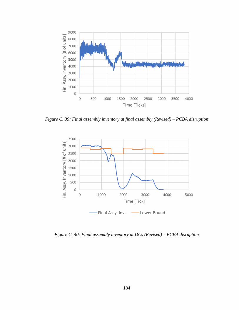
184
Figure C. 39: Final assembly inventory at final assembly (Revised) – PCBA disruption
Figure C. 40: Final assembly inventory at DCs (Revised) – PCBA disruption

185
D Simulation User Guide
D.1 Overview of Data Input Files
Before opening the NetLogo model, several data input files should be updated and saved.
Each of the following input files should be saved in the same folder as the main NetLogo
(.nlogo) file. The data should be edited in the Excel workbook “network_Lexmark(7)” and
copied into the appropriate text files.
initial.txt
Most of the inputs to the simulation model are read from the text file “initial.txt”. The
information is edited in the Excel worksheet titled “initial node vars.” Table D. 1 describes
all the data input categories that must be completed in this initialization file. Each variable
must be assigned a value for each node-type agent. Each variable must be assigned a value
even if the corresponding node-type agent is to remain inactive throughout the simulation.
For example, the main fuser node, the secondary fuser node, and the alternate fuser node
must be assigned an initial displays inventory of 0 at initialization although its value will
not change since no displays are ever sent to or requested from the fuser node.
Table D. 1: Node initialization variables
Variable Name Description
"inv_DIS" Inventory of displays at simulation start
"inv_ASI" Inventory of ASICS at simulation start
"inv_POW" Inventory of power supplies at simulation start
"inv_DCM" Inventory of DC motors at simulation start
"inv_FUS" Inventory of fusers at simulation start
"inv_PAC" Inventory of packaging materials at simulation start
"inv_LSU" Inventory of LSUs at simulation start
"inv_SCA" Inventory of scanners at simulation start
"inv_PHO" Inventory of photoconductors at simulation start
"inv_PLA1" Inventory of plastic parts (for main printer assembly) at simulation start
"inv_PLA2" Inventory of plastic parts (for toner cartridge) at simulation start

186
Table D. 1 continued
Variable Names Descriptions
"inv_GEA1" Inventory of gears (for main printer assembly) at simulation start
"inv_GEA2" Inventory of gears (for toner cartridge) at simulation start
"inv_TON" Inventory of toner at simulation start
"inv_PCB" Inventory of PCBAs at simulation start
"inv_CAR" Inventory of toner cartridges at simulation start
"inv_FIN" Inventory of final assemblies at simulation start
"full_cap" Full production capacity of the node, maximum the node can output in 1 tick
"full_cap2" Full production capacity of the node for secondary production type (only needed for gears and plastic parts nodes which have 2 types of production)
"hidden?" True if node is visible (active) and False otherwise
"actives" # of active trucks (not including hidden trucks) at the node
"doh" desired on-hand inventory
"doh2" desired on-hand inventory of secondary type (only needed for nodes which make 2 part types)
"buf1" The lowest amount of inventory desired of raw material type 1, type of material depends on the node
"buf2" The lowest amount of inventory desired of raw material type 2
"buf3" The lowest amount of inventory desired of raw material type 3
"buf4" The lowest amount of inventory desired of raw material type 4
"buf5" The lowest amount of inventory desired of raw material type 5
"buf6" The lowest amount of inventory desired of raw material type 6
"buf7" The lowest amount of inventory desired of raw material type 7
"buf8" The lowest amount of inventory desired of raw material type 8
"buf9" The lowest amount of inventory desired of raw material type 9
"buf10" The lowest amount of inventory desired of raw material type 10
"buf11" The lowest amount of inventory desired of raw material type 11
"full_alloc" % of order allocated to node when it is operating at full capacity
"reg_mat cost" cost of materials per unit during normal operation
"dis_mat_cost" cost of materials per unit during disruption
"ramp" the rate at which capacity increases to reach its full capacity from a diminished state, as in after disruption or upon startup
"disruption?" True if the node will experience a disruption, False otherwise
"dis_start" Tick count at which the disruption begins
"dis_duration" Number of ticks the disruption lasts
"alt_startup_delay" Number of ticks that must elapse before the alternate supplier can activate once it has been signaled to open
"Vis?" True if the node has visibility into its buyers’ production rate
"severity" percentage of capacity lost when a node is disrupted

187
truck_cor.txt
The file “truck_cor.txt” file also contains initialization data for truck-type agents including
the starting coordinates for the truck-type agents, and whether they should be hidden and
inactive. Any time the “initial.txt” file is updated, the truck-type agent information should
also be updated in the “truck_cor.txt” file. For example, if a node was using dual sourcing
in one scenario, but the strategy was later changed to single sourcing, both the “initial” and
“truck_cor” files should be updated to reflect this. Information is edited in the Excel
worksheet “new truck cor.” Table D. 2 describes all the data input categories that must be
completed in this initialization file. It is important to update the “initial node vars”
worksheet before copying the data from “new truck cor” since some values are referenced
between the two sheets.
Table D. 2: Truck initialization variables
Variable Name Description
x cor X coordinate for truck starting position
y cor Y coordinate for truck starting position
truckload Maximum number of units a truck can carry
truck hidden? True if truck is hidden and inactive, False otherwise
speed
Truck speed, represented by the coordinate distance that can be covered in one tick, value updates each tick based on random-normal to reflect travel time variability
geo distance The magnitude of transportation time expected between nodes, reflected on a 1-3 scale with 1 corresponding to the shortest time
link lengths Cartesian distance between two connected nodes
Mu Average # of ticks the truck will require to cover the distance to its destination
TT_sigma Standard deviation of # of ticks the truck will require to cover the distance to its destination
cor.txt
The “cor.txt” file contains the coordinates for each node-type agent. These include
suppliers, the final printer assembly, and distribution centers. The file also contains the
names of each node which will appear next to the node in the simulation interface. This
information is only input once when the network configuration is defined. The coordinates
are set up to evenly distribute the nodes and to avoid the crossing of links between nodes.

188
The transportation time between nodes is not affected by the cartesian distance between
nodes, but instead is controlled by adjusting the speed of the truck-type agents in proportion
to the distance that must be covered in the simulation space. Information is edited in the
excel worksheet “coordinates.” Table D. 3 describes the data required for the “cor.txt” file.
Table D. 3: Node coordinate variables
Variable Name Description
x-cor X coordinate for node position
y-cor Y coordinate for node position
name Name to be displayed next to the node, eg. “Displays”
network.txt
The “network.txt” file defines the linkages between nodes. It is oriented in the form of a
from-to matrix. If a 1 is found in the matrix, a directed link is made from the node listed in
the row to the node listed in the intersecting column. If a 0 is found, no link is made. After
the initial setup, this information is not changed. Links may hide or unhide in coordination
with the status of the connected nodes. The information is input in the excel worksheet
“links from to.” An example from-to matrix is displayed in Table D. 4. The displays nodes
are not linked to the toner nodes, while they are linked to the PCBA nodes. Each node
name has three instances in the rows and columns corresponding with the primary,
secondary, and alternate suppliers.
Table D. 4: Example from-to matrix for network setup
Ton
er
Ton
er
Ton
er
PC
BA
PC
BA
PC
BA
0 Displays 0 0 0 1 1 1
1 Displays 0 0 0 1 1 1
2 Displays 0 0 0 1 1 1

189
demand.txt
As shown in Table D. 5, the “demand.txt” file contains the demand during each period of
the simulation for final printer assemblies (FIN), toner cartridges (CAR), and
photoconductors (PHO). The file also contains the forecast demand for the next period, one
period ahead of the current demand, which the distribution centers use to place orders. The
information is edited in the excel worksheet “Demand_extended.” In each case the demand
values are taken as the average of a normally distributed variable, and the actual demand
during each cycle is sampled from the distribution. The forecast value is assumed equal to
the average of the demand distribution, and is always read once cycle ahead of the demand.
The average demand varies from quarter to quarter, but remain constant within each
quarter. Sufficient data should be input to last for a two-year run period.
Table D. 5: Example demand data
DC1
quarter day FIN forecast CAR forecast PHO forecast
1 1 tick 8 cycle 1 0 336 0 672 0 134.4
1 2 tick 16 cycle 2 336 336 672 672 134.4 134.4
1 3 tick 24 cycle 3 336 336 672 672 134.4 134.4
1 4 tick 32 cycle 4 336 336 672 672 134.4 134.4
.
.
.
4 479 tick 3832 cycle 479 480 336 960 672 192 134.4
Two use cases for the simulation are described. First, a one-time simulation run is
performed with no disruptions. The one-time run does not output any data files, but is
useful for troubleshooting and demonstration. Next, a multi-replication run is performed
for a disruption scenario. For the multi-replication case, the built-in BehaviorSpace tool is
used to output the KPI data at each tick to a csv file which can is then used for plotting in
Excel.

190
D.2 Simulation Use-Case 1: Single run with no disruptions
1. “disruption?” column in initial node vars worksheet should read FALSE for all
nodes.
a. No disruptions should occur in this scenario
2. Copy current data into “initial.txt” and “truck_cor.txt”
a. Copy only data, no column or row header information
b. Do not copy data highlighted in yellow, which is for reference only
3. Open NetLogo file, “Printer_SC_rev26_baselinebounds_extended_revD” or
“Printer_SC_rev27_revisedbounds_extended_revD” corresponding to the input
data
a. “Baselinebounds” is set up for the baseline segmentation method, and
“Revisedbounds” is set up for the revised segmentation method
b. The two NetLogo files, “Baselinebounds” and “Revisedbounds” differ in
the values for normal operating bounds, which can be noted in the check-
RR procedure in the code tab and in the moving average plots, as in Figure
D. 1, found in the bottom right of the simulation interface
c. Files also differ in network setup and node capacity
d. Static dataset can be copied from worksheets “initial Revised_Scaled” or
“initials Baseline_Scaled” into “intial_node_vars”
e. Any temporary data changes should only be made in “initial_node_vars”
sheet

191
Figure D. 1: Moving average plot with cartridge inventory lower bound
4. Press setup button or shift+S to setup node and truck agents
5. Pres setup-links button or shift+L to setup links
a. Simulation interface upon opening is shown in Figure D. 2.
Figure D. 2: Simulation interface upon opening with startup command button highlighted
6. Ensure all trucks are matched with node locations, overlaying yellow house icons
a. Initial simulation setup with correct truck and node location demonstrated
in Figure D. 3

192
Figure D. 3: Simulation interface showing initial node and truck setup

193
7. Ensure all nodes are connected with links
a. Trucks not initialized at an active node location indicates “initial.txt” and/or
“truck_cor.txt” file needs to be updated
8. Press go button or shift+G
9. Adjust simulation speed with “normal speed” slider
a. Mid-range speed is recommended for observing truck behavior and data
monitors during troubleshooting
10. For fastest results, maximize the speed slider and turn off “view updates”
11. Simulation will terminate after 2 year run time
a. Should take approximately five minutes using full speed and no animation
updates
12. Observe simulation output
a. Scroll to far bottom-right in the simulation window to view plots of KPI
along with the calculated lower or upper bounds, highlighted in red in
Figure D. 4
b. Observe other plots which include inventory, capacity, and order allocation
plots for each node
Figure D. 4: Full simulation interface showing all plots and data monitors

194
D.3 Simulation Use-Case 2: Multi-replication run with a disruption
1. “disruption?” column in initial node vars worksheet should read TRUE for one
node which experiences the disruption
a. Disruption should occur at a primary supplier
b. Also specify disruption start time, duration, and severity
c. Data inputs for disruption scenario highlighted in Table D. 6
Table D. 6: Initialization data highlighting inputs for disruption scenario
"disruption?" "dis_start" "dis_duration" "alt_startup_delay" "Vis?"
"severity" 0=no capacity; .5=half capacity; 1=full capacity
“Displays” TRUE 720 480 0 FALSE 0
“Displays 2” FALSE 3354 0 0 FALSE 1
“Displays Alt” FALSE 3354 0 480 FALSE 1
2. Copy current data into “initial.txt” and “truck_cor.txt” and open NetLogo file as in
previous use-case scenario
3. Open BehaviorSpace in the tools menu or Ctrl+Shift+B
a. BehaviorSpace menu opens with previous experimental setups, as in Figure D.
5

195
Figure D. 5: BehaviorSpace menu
4. Click edit experiment named “disruption scenarios”
a. Experiment will run thirty replications and output KPI data at every tick
b. “disruption scenarios” settings are shown in Figure D. 6

196
Figure D. 6: disruption scenarios experimental setup
5. Click OK and Run
a. Select spreadsheet output, as in Figure D. 7
b. Keep standard, 4 simultaneous simulation runs in parallel
c. Select name and location for output .csv file
These variables
will output to .csv
file
Each variable gives its value
at the end of each tick
Experiment will output data
from 30 simulation runs

197
Figure D. 7: BehaviorSpace run options
6. Conduct any additional data formatting and plotting by opening .csv in Excel
a. After formatting, save as Excel type file
198
References
1. Abyaneh, M., S. Hassanzadeh and H. Raddum (2011). Tutorial paper on
quantitative risk assessment. Norsk Informatikkonferanse. University of Tromso.
2. Adenso-Diaz, B., C. Mena, S. García-Carbajal and M. Liechty (2012). "The impact
of supply network characteristics on reliability." Supply Chain Management 17(3):
263-276.
3. Albino, V., N. Carbonara and I. Giannoccaro (2007). "Supply chain cooperation in
industrial districts: A simulation analysis." European Journal of Operational
Research 177(1): 261-280.
4. Alcantara, P. (2014). Supply chain trends: past, present and future, Business
Continuity Institute.
5. Ambulkar, S., J. Blackhurst and S. Grawe (2015). "Firm's resilience to supply chain
disruptions: Scale development and empirical examination." Journal of Operations
Management 33-34: 111-122.
6. Basole, R. C. and M. A. Bellamy (2014). "Visual analysis of supply network risks:
Insights from the electronics industry." Decision Support Systems 67: 109-120.
7. Behdani, B. (2012). Evaluation of paradigms for modeling supply chains as
complex socio-technical systems. Simulation Conference (WSC), Proceedings of
the 2012 Winter, IEEE.
8. Behdani, B., Z. Lukszo, A. Adhitya and R. Srinivasan (2010). "Performance
analysis of a multi-plant specialty chemical manufacturing enterprise using an
agent-based model." Computers and Chemical Engineering 34(5): 793-801.
9. Bensaou, M. (1999). "Portfolios of buyer-supplier relationships." Sloan
Management Review 40(4): 35-44.
10. Blackhurst, J., C. W. Craighead, D. Elkins and R. B. Handfield (2005). "An
empirically derived agenda of critical research issues for managing supply-chain
disruptions." International Journal of Production Research 43(19): 4067-4081.
11. Blackhurst, J., K. S. Dunn and C. W. Craighead (2011). "An Empirically Derived
Framework of Global Supply Resiliency." Journal of Business Logistics 32(4):
374-391.
12. Boone, C. A., C. W. Craighead, J. B. Hanna and A. Nair (2013). "Implementation
of a System Approach for Enhanced Supply Chain Continuity and Resiliency: A
Longitudinal Study." Journal of Business Logistics 34(3): 222-235.
13. Brandon-Jones, E., B. Squire, C. W. Autry and K. J. Petersen (2014). "A Contingent
Resource-Based Perspective of Supply Chain Resilience and Robustness." Journal
of Supply Chain Management 50(3): 55-73.
14. Brown, A. and F. Badurdeen (2015). Increased Supply Chain Resilience through
Consideration of Disruption Impact Severity in the Supplier Segmentation Process
Industrial and Systems Engineering Research Conference. Nashville, Tennessee.
15. Caridi, M., R. Cigolini and D. De Marco (2005). "Improving supply-chain
collaboration by linking intelligent agents to CPFR." International Journal of
Production Research 43(20): 4191-4218.

199
16. Carter, J. R. and R. Narasimhan (1996). "Purchasing and supply management:
Future directions and trends." International Journal of Purchasing and Materials
Management Fall 1996.
17. Chiang, C.-Y., C. Kocabasoglu-Hillmer and N. Suresh (2012). "An empirical
investigation of the impact of strategic sourcing and flexibility on firm's supply
chain agility." International Journal of Operations & Production Management
32(1): 49-78.
18. Christopher, M. and H. Peck (2004). "Building the Resilient Supply Chain."
International Journal of Logistics Management 15(2): 1-13.
19. Coate, M. B. (1983). "Pitfalls in portfolio planning." Long Range Planning 16(3):
47-56.
20. Craighead, C. W., J. Blackhurst, M. J. Rungtusanatham and R. B. Handfield (2007).
"The Severity of Supply Chain Disruptions: Design Characteristics and Mitigation
Capabilities." Decision Sciences 38(1): 131-156.
21. Croxton, K. L., S. J. Garcia-Dastugue and D. M. Lambert (2001). "Supply chain
management processes." The International Journal of Logistics Management 12(2):
13-36.
22. Day, M., G. M. Magnan and M. M. Moeller (2010). "Evaluating the bases of
supplier segmentation: A review and taxonomy." Industrial Marketing
Management 39: 625-639.
23. de Santa-Eulalia, L. A., S. D'Amours and J. Frayret (2010). Modeling agent-based
simulations for supply chain planning: The FAMASS methodological framework.
Systems Man and Cybernetics (SMC), 2010 IEEE International Conference on.
24. de Santa Eulalia, L. A. (2009). Agent-based simulations for advanced supply chain
planning: a methodological framework for requirements analysis and deployment,
UNIVERSITÉ LAVAL QUÉBEC.
25. Denyer, D. and D. Tranfield (2009). Producing a systematic review. The Sage
handbook of organizational research methods. D. A. B. A. Bryman. Thousand
Oaks, CA, Sage Publications Ltd: 671-689.
26. Dubois, A. and A.-C. Pederson (2002). "Why relationships do not fit into
purchasing portfolio models - a comparison between the portfolio and indsutrial
network approaches." European Journal of Purchasing & Supply Management 8:
35-42.
27. Durach, C. F., A. Wieland and J. A. D. Machuca (2015). "Antecedents and
dimensions of supply chain robustness: a systematic literature review."
International Journal of Physical Distribution & Logistics Management 45(1/2):
118-137.
28. Dyer, J. H., D. S. Cho and W. Chu (1998). "Strategic supplier segmentation: The
next "best practice" in supply chain management." California Management Review
40(2): 57-77.
29. Dyer, J. H., Singh, H. (1998). "The relational view: Cooperative strategy and
sources of interorganizational competitive advantage." The Academy of
Management Review 23(4): 660-679.
30. Ellis, S. C., R. M. Henry and J. Shockley (2010). "Buyer perceptions of supply
disruption risk: A behavioral view and empirical assessment." Journal of
Operations Management 28(1): 34-46.

200
31. Fine, C. H. (1999). Clockspeed: Winning Industry Control in the Age of Temporary
Advantage. USA, Basic Books.
32. Forget, P., S. D’Amours and J.-M. Frayret (2008). "Multi-behavior agent model for
planning in supply chains: An application to the lumber industry." Robotics and
Computer-Integrated Manufacturing 24(5): 664-679.
33. Fox, M. S., J. F. Chionglo and M. Barbuceanu (1993). "The integrated supply chain
management sysem." Internal Report, Department of Industrial Engineering
University of Toronto.
34. Gaudreault, J., P. Forget, J.-M. Frayret, A. Rousseau, S. Lemieux and S. D'Amours
(2010). "Distributed operations planning in the softwood lumber supply chain:
Models and coordination." International Journal of Industrial Engineering : Theory
Applications and Practice 17(3): 168-189.
35. Gelderman, C. J. and A. J. v. Weele (2005). "Purchasing portfolio models: A
critique and update." The Journal of Supply Chain Management Summer 2005:
19-28.
36. Giannakis, M. and M. Louis (2011). "A multi-agent based framework for supply
chain risk management." Journal of Purchasing & Supply Management 17(1): 23-
31.
37. Golgeci, I. and S. Y. Ponomarov (2013). "Does firm innovativeness enable
effective responses to supply chain disruptions? An empirical study." Supply Chain
Management 18(6): 604-617.
38. Greening, P. and C. Rutherford (2011). "Disruptions and supply networks: a multi-
level, multi-theoretical relational perspective." International Journal of Logistics
Management 22(1): 104-126.
39. Hadeler, B. J. and J. R. Evans (1994). "Supply strategy: Capturing the value."
Strategic Alliances July/August 1994: 3-4.
40. Hallikas, J., K. Puumalainen, T. Vesterinen and V.-M. Virolainen (2005). "Risk-
based classifcation of supplier relationships." Journal of Purchasing & Supply
Managment 11: 72-82.
41. Hearnshaw, E. J. S. and M. M. J. Wilson (2013). "A complex network approach to
supply chain network theory." International Journal of Operations & Production
Management 33(4): 442-469.
42. Hohenstein, N.-O., E. Feisel, E. Hartmann and L. Giunipero (2015). "Research on
the phenomenon of supply chain resilience." International Journal of Physical
Distribution & Logistics Management 45(1/2): 90-117.
43. Hou, Y. Z., Z. H. Sheng and X. L. Wang (2008). Research of Buyer-Supplier
Relationship Based on Agent Approach. Wireless Communications, Networking
and Mobile Computing, 2008. WiCOM '08. 4th International Conference on.
44. Hulsmann, M., J. Grapp and Y. Li (2008). "Strategic adaptivity in global supply
chains-Competitive advantage by autonomous cooperation." International Journal
of Production Economics 114(1): 14-26.
45. ISO (2009). International stadards oranization standard on risk management.
31000. Geneva.
46. Janssen, M. (2005). "The architecture and business value of a semi-cooperative,
agent-based supply chain management system." Electronic Commerce Research
and Applications 4(4): 315-328.

201
47. Jusko, J. (2008). Kraft crafts an open innovation strategy. Industry Week.
December 2008: 60-61.
48. Jüttner, U. and S. Maklan (2011). "Supply chain resilience in the global financial
crisis: an empirical study." Supply Chain Management 16(4): 246-259.
49. Kapucu, N. and M. Van Wart (2006). "THE EVOLVING ROLE OF THE PUBLIC
SECTOR IN MANAGING CATASTROPHIC DISASTERS: Lessons Learned."
Administration & Society 38(3): 279-308.
50. Kaufman, A., C. H. Wood and G. Theyel (2000). "Collaboration and technology
linkages: A strategic supplier typology." Strategic Management Journal 21: 649-
663.
51. Kleindorfer, P. R. and G. H. Saad (2005). "Managing Disruption Risks in Supply
Chains." Production & Operations Management 14(1): 53-68.
52. Klibi, W., A. Martel and A. Guitouni (2010). "The design of robust value-creating
supply chain networks: A critical review." European Journal of Operational
Research 203: 283-293.
53. Klibi, W., A. Martel and A. Guitouni (2010). "The design of robust value-creating
supply chain networks: A critical review." European Journal of Operational
Research 203(2): 283-293.
54. Kovács, G. (2009). "Identifying challenges in humanitarian logistics." International
Journal of Physical Distribution & Logistics Management 39(6): 506-528.
55. Kraljic, P. (1983). "Purchasing must become supply management." Harvard
Business Review September-October 1983: 109-117.
56. Lambert, D. M. (2006). Supply Chain Management: Processes, Partnerships,
Performance. USA, Supply Chain Management Institute.
57. Lambert, D. M., M. A. Emmelhainz and J. T. Gardner (1996). "Developing and
implementing supply chain partnerships." The International Journal of Logistics
Management 7(2): 1-18.
58. Lee, J. H. and C. O. Kim (2007). "Multi-agent systems applications in
manufacturing systems and supply chain management: a review paper."
International Journal of Production Research 46(1): 233-265.
59. Li, J. and F. T. S. Chan (2012). "The impact of collaborative transportation
management on demand disruption of manufacturing supply chains." International
Journal of Production Research 50(19): 5635-5650.
60. Mandal, S. (2012). "An Empirical Investigation into Supply Chain Resilience." IUP
Journal of Supply Chain Management 9(4): 46-61.
61. Markowitz, H. (1952). "Portfolio Selection." Journal of Finance 7(1): 77-91.
62. Melnyk, S. A., E. W. Davis, R. E. Spekman and J. Sandor (2010). "Outcome-Driven
Supply Chains." MIT Sloan Management Review 51(2): 33-38.
63. Mohebbi, S. and X. Li (2012). "Designing intelligent agents to support long-term
partnership in two echelon e-Supply Networks." Expert Systems with Applications
39(18): 13501-13508.
64. Nair, A. and J. M. Vidal (2011). "Supply network topology and robustness against
disruptions - An investigation using multi-agent model." International Journal of
Production Research 49(5): 1391-1404.

202
65. North, M. J. and C. M. Macal (2007). Managing Business Complexity: Discovering
Strategic Solutions with Agent-Based Modeling and Simulation. New York, New
York, Oxford University Press.
66. Oehmen, J. and E. Rebentisch (2010). "Risk management in lean PD." LAI Paper
Series" Lean Product Development for Practitioners.
67. Ojha, D., P. T. Gianiodis and I. Manuj (2013). "Impact of logistical business
continuity planning on operational capabilities and financial performance."
International Journal of Logistics Management 24(2): 180-209.
68. Oki Data Systems, I. (2007). Retrieved July 31, 2017, from
http://www.fireballpc.com/Laser_Printer_Information.html.
69. Olcott, G. and N. Oliver (2014). "Social Capital, Sensemaking, and Recovery:
Japanese Companies and the 2011 Earthquake." California Management Review
56(2): 5-22.
70. Olsen, R. F. and L. M. Ellram (1997). "A portfolio approach to supplier
relationships." Industrial Marketing Management 26: 101-113.
71. Peck, H. (2005). "Drivers of supply chain vulnerability: an integrated framework."
International Journal of Physical Distribution & Logistics Management 35(4): 210-
232.
72. Persson, G. and H. Hakansson (2007). "Supplier segmentation “when supplier
relationships matter”." The International Marketing and Purchasing Journal 1(3):
26-41.
73. Pettit, T. J., K. L. Croxton and J. Fiksel (2013). "Ensuring Supply Chain Resilience:
Development and Implementation of an Assessment Tool." Journal of Business
Logistics 34(1): 46-76.
74. Ponis, S. T. and E. Koronis (2012). "A Knowledge Management Process-Based
Approach to Support Corporate Crisis Management." Knowledge & Process
Management 19(3): 148-159.
75. Revilla, E. and M. J. Sáenz (2014). "Supply chain disruption management: Global
convergence vs national specificity." Journal of Business Research 67(6): 1123-
1135.
76. Reynolds, C. (2007). "Boids: Background and Update." Retrieved September 11,
2015, from http://www.red3d.com/cwr/boids/.
77. Rezaei, J. and R. Ortt (2012). "A multi-variable approach to supplier
segmentation." International Journal of Production Research 50(16): 4593-4611.
78. Rijt, J. and S. C. Santerna (2010). A conceptual model for interactions between
suppliers and buyers: from uni-faced to multi-faced B2B sales organizations.
International IPSERA workshop on Customer attractiveness, supplier satisfaction
and customer value. University of Twente.
79. Ritter, T. (2000). "A framework for analyzing interconectedness of relationships."
Industrial Marketing Management 29: 317-326.
80. Scholten, K., P. S. Scott and B. Fynes (2014). "Mitigation processes – antecedents
for building supply chain resilience." Supply Chain Management 19(2): 211-228.
81. Shambro, L. (2010). Maximizing long term "cost savings" (=Value). Contract
Manufacturing & Packaging. November/December 2010: 6-7.

203
82. Shao, X.-F. (2013). "Supply chain characteristics and disruption mitigation
capability: an empirical investigation in China." International Journal of Logistics:
Research & Applications 16(4): 277-295.
83. Sheffi, Y. (2009). Business Continuity: A Systematic Approach. Global Business
and the Terrorist Threat. Cheltenham, UK, 'Edward Elgar Publishing, Inc.'.
84. Sheffi, Y. and J. B. Rice Jr (2005). "A Supply Chain View of the Resilient
Enterprise." MIT Sloan Management Review 47(1): 41-48.
85. Shen, W., Q. Hao, H. J. Yoon and D. H. Norrie (2006). "Applications of agent-
based systems in intelligent manufacturing: An updated review." Advanced
Engineering Informatics 20(4): 415-431.
86. Sterman, J. D. (1989). "Modeling managerial behavior: Misperceptions of feedback
in a dynamic decision making experiment." Management Science 35(3): 321-339.
87. Supply Chain Council, I. (2006). "Supply-Chain Operations Reference-model
(SCOR) - Version 8.0."
88. Suzuki, Y. (2012). "Disaster-Relief Logistics With Limited Fuel Supply." Journal
of Business Logistics 33(2): 145-157.
89. Tang, C. S. (2006). "Robust strategies for mitgating supply chain disruptions."
International journal of Logistics: Research and Applications 9(1): 33-45.
90. Tang, O. and S. N. Musa (2011). "Identifying risk issues and research
advancements in supply chain risk management." International Journal of
Production Economics 133(1): 25-34.
91. Thompson, J. D. (1967). Organizations in Action, McGraw Hill, Inc.
92. Turnbull, P. W. (1990). "A review of portfolio planning models for industrial
marketing and purchasing management." European Journal of Marketing 24(3): 7-
22.
93. Upton, E. and W. J. Nuttall (2014). "Fuel panics: Insights from spatial agent-based
simulation." IEEE Transactions on Intelligent Transportation Systems 15(4): 1499-
1509.
94. Venkateswaran, A., K. Simon-Agolory and K. Z. Watkins (2014). "Long term
recovery from mega-disasters: regional and business recovery periods, differential
vulnerability, and business continuity." International Journal of Risk Assessment
& Management 17(4): 332-360.
95. Wieland, A. and C. M. Wallenburg (2013). "The influence of relational
competencies on supply chain resilience: a relational view." International Journal
of Physical Distribution & Logistics Management 43(4): 300-320.
96. Wu, T., S. Huang, J. Blackhurst, X. Zhang and S. Wang (2013). "Supply Chain
Risk Management: An Agent-Based Simulation to Study the Impact of Retail
Stockouts." IEEE Transactions on Engineering Management 60(4): 676-686.
97. Yusuf, Y. Y., A. Musa, M. Dauda, N. El-Berishy, D. Kovvuri and T. Abubakar
(2014). "A study of the diffusion of agility and cluster competitiveness in the oil
and gas supply chains." International Journal of Production Economics 147(Part
B): 498-513.
98. Zsidisin, G. A., S. A. Melnyk and G. L. Ragatz (2005). "An institutional theory
perspective of business continuity planning for purchasing and supply
management." International Journal of Production Research 43(16): 3401-3420.

204
99. Zsidisin, G. A. and B. Ritchie (2009). Supply Chain Risk: A Handbook of
Assessment, Management, and Performance. New York, NY, USA, Springer.
100. Zsidisin, G. A. and S. M. Wagner (2010). "Do Perceptions Become Reality?
The Moderating Role of Supply Chain Resiliency on Disruption Occurrence."
Journal of Business Logistics 31(2): 1-20.

205
VITA
Name
Adam J. Brown
Place of Birth
Princeton, Kentucky
Education
B.S. Mechanical Engineering, University of Kentucky
M.S. Manufacturing Systems Engineering, University of Kentucky
Professional Experience
Research Assistant, University of Kentucky Institute for Sustainable
Manufacturing
Teaching Assistant, University of Kentucky Department of Mechanical
Engineering
Co-Op, GE Aviation in Madisonville, KY
Honors/Awards
Manufacturing & Design Division Best Track Paper, 3rd Place, 2017 Institute for
Industrial and Systems Engineers (IISE) Annual Conference, Pittsburgh, PA
Outstanding student poster award, University of Kentucky Mechanical
Engineering 2017 Student Research Showcase
Cincinnati Roundtable Council of Supply Chain Management Professionals
(CSCMP) Scholarship to attend 2015 CSCMP Annual Conference, San Diego,
CA
NSF Student Travel Grant for 2015 International Congress on Sustainability
Science and Engineering (ICOSSE), Balatonfured, Hungary
University of Kentucky Graduate School Travel Grant to attend 2015 Industrial
Systems and Engineering Research Conference (ISERC), Nashville, TN
Systems Engineering Division Best Paper Award, 2014 American Society for
Engineering Education Annual Conference (ASEE), Indianapolis, IN

206
University of Kentucky Graduate School Travel Grant to attend 2014 Industrial
Systems and Engineering Research Conference (ISERC), Montreal, Canada
Operations Research, Systems Engineering, and Industrial Engineering Commons
2013 – One of Most Downloaded Theses
NSF Student Travel Grant for 2013 IEEE Conference on Automation Science and
Engineering (CASE), Madison, WI
2013 E.Wayne Kay Graduate Scholarship, Society of Manufacturing Engineers-
Education Foundation
Student Research Poster Award, 2nd place, 2013 Third International Forum on
Sustainable Manufacturing, University of Kentucky
Conference Paper Award, Honorable Mention. 2011 IEEE International
Conference on Industrial Engineering and Engineering Management (IEEM),
Singapore
2010 Dr. Karl Otto Lange Memorial Fellowship
Journal Publications
1. Brown, A., Amundson, J., Badurdeen, F., 2014, “Sustainable Value
Stream Mapping (Sus-VSM) in Different Manufacturing System
Configurations: Application Case Studies”, Journal of Cleaner
Production, 85(15), pp. 164-179
2. Badurdeen, F., Shuaib, M., Wijekoon, K., Brown, A., Faulkner, W.,
Amundson, J., Jawahir, I. S., Goldsby, T., Iyengar, D., and Boden, B.,
2014, “Quantitative Modeling and Analysis of Supply Chain Risks using
Bayesian Theory,” Journal of Manufacturing Technology Management,
25(5), pp. 631-654
3. Brown, A., Badurdeen, F., “Structured Literature Review Supporting
Development of a Resilience-Oriented Supplier Segmentation Method”,
pending submission to the European Journal of Logistics, Purchasing,
and Supply Chain Management

207
Working Papers
1. Agent-Based Model and Simulation Examining the Effects of Supplier
Segmentation on Resilience and Robustness, In preparation for
submission to the Journal of Supply Chain Management
2. Development of a Resilience-Enabling Supplier Segmentation Method,
In preparation for submission to the Journal of Purchasing & Supply
Management
Conference Papers
1. Brown, A., & Badurdeen, F., (2017). Supplier Segmentation Method for
Selection of Resilience-Enabling Procurement Strategies. Paper
accepted for presentation at the Industrial Systems and Engineering
Research Conference (ISERC), May 20 – 23, Pittsburgh, PA.
* Manufacturing & Design Division Best Track Paper, 3rd Place
2. Aydin, R., Brown, A., Ali, A., & Badurdeen, F., (2017). Assessment of
End-of-life Product Lifecycle ‘ilities’. Paper accepted for presentation
at the Industrial Systems and Engineering Research Conference
(ISERC), May 20-23, Pittsburgh, PA.
3. Brown, A., & Badurdeen, F., (2015). Increased Supply Chain
Resilience through Consideration of Disruption Impact Severity in the
Supplier Segmentation Process. Presented at the Industrial Systems and
Engineering Research Conference (ISERC), May 30 – June 2, 2015,
Nashville, TN.
4. Badurdeen, F., Baker, J.R., Rouch, K.E., Goble, K.E., Swan, G.M.,
Brown, A., & Jawahir I.S., (2015). Development of an Online Master's
Degree Program in Manufacturing Systems Engineering. Proc. 122nd
ASEE Annual Conference and Exposition, Seattle, WA, USA, June 14-
17, 2015.
5. Badurdeen, F., Sekulic, D., Gregory, B., Brown, A., & Fu, H., (2014).
Developing and Teaching a Multidisciplinary Course in Systems
Thinking for Sustainability: Lessons Learned through Two Iterations.
Presented at the 121st Annual American Society for Engineering
Education Annual Conference & Exposition, June 15-18, 2014,
Indianapolis, IN. *Systems Engineering Division Best Paper Award
6. Brown, A., & Badurdeen, F., (2014). Supply Chain Disruption
Management: Review of Issues and Research Directions. Presented at
the Industrial Systems and Engineering Research Conference (ISERC),
May 31 – June 3, 2014, Montreal, Canada.
7. Amundson, J., Brown, A., Grabowski, M., & Badurdeen, F., (2014).
Life-cycle risk modeling: alternate methods using Bayesian Belief
Networks. Procedia CIRP, Vol. 17, 2014, pp: 320-325.

208
8. Brown, A., & Badurdeen, F., (2013). A queuing model for systems with
rework and process downtime. (2013). Presented at the IEEE
International Conference on Automation Science and Engineering
(CASE), Aug. 17-21, 2013, Madison, WI.
9. Brown, A, Amundson, J., & Badurdeen, F., (2013). Bayesian Informed
Simulation for Supply Chain Risk Probability and Impact Assessment.
Presented at the International Conference on Production Research
(ICPR), July 28-August 1, 2013, Iguazu Falls, Brazil.
10. Amundson, J., Brown, A., Shuaib, M., Badurdeen, F., & Goldsby, T.,
(2013). Bayesian Methodology for Supply Chain Risk Analysis: Concept
and Case Studies. Presented at the Industrial and Systems Engineering
Research Conference (ISERC), May 18-22, 2013, San Juan, Puerto
Rico.
11. Badurdeen, F., A. Brown, R. Gregory, H. Fu, M. Schroeder, D. Sekulic,
L. Vincent, & G. A. Luhan, (2013). Reframing Interdisciplinary
Approaches to Systems Thinking for Sustainability. Proc. International
Symposium on Sustainable Systems & Technologies (ISSST), May 15
– 17, 2013, Cincinnati, OH USA.
12. Brown, A., & Badurdeen, F., (2011). Optimization of queuing theory
wait time through multi-skilled worker assignments. Presented at the
IEEE International Conference on Industrial Engineering and
Engineering Management (IEEM), Dec. 6-9, 2011. *Conference paper
award, honorable mention
Conference Presentations with Refereed Abstracts
1. Aydin, R., Brown, A. & Badurdeen, F., (2017). Total Lifecycle Product
Design Optimization, Submitted for the International Congress on
Sustainability Science and Engineering (ICOSSE '17), October 2-4,
2017, Barcelona, Spain.
2. Amundson, J., Badurdeen, F., & Brown, A., (2015). Quantitative
modeling to assess total life-cycle risk implications across the supply
chain for sustainable manufacturing decision making. Presented at the
International Congress on Sustainability Science and Engineering
(ICOSSE), Balatonfured, Hungary, May 26-29, 2015.
3. Badurdeen, F., A. Brown, J. Amundson, & S. Roberts, (2013).
Manufacturing Sustainability Evaluation through Sustainable Value
Stream Mapping (Sus-VSM): Approach and Case Study. Presented at
the International Congress on Sustainability Science and Engineering
(ICOSSE), August 11-15, 2013, Cincinnati, OH.
4. Badurdeen, F., Gregory, R., Luhan, G., Schroder, M., Sekulic, D.,
Vincent, L., Brown, A. & Fu, H., (2013). Systems Thinking for
Sustainability: Experiences from Developing and Teaching a Multi-

209
disciplinary Course. Presented at the Kentucky Innovations
Conference, May 16-17, 2013, Lexington, KY, USA.
Posters
1. Brown, A., & Badurdeen, F., (2017). Resilience Assessment in the
Context of a Laser Printer Supply Chain: Comparison of Two Supplier
Segmentation Methods. Presented at the University of Kentucky
Mechanical Engineering Student Research Showcase, Lexington, KY.
*Outstanding student poster award
2. Brown, A., & Badurdeen, F., (2017). Resilience Assessment in the
Context of a Laser Printer Supply Chain: Comparison of Two Supplier
Segmentation Methods. Presented at the University of Kentucky Gatton
College of Business and Economics 7th Annual Supply Chain Forum:
Managing Risks in the Supply Chain
3. Brown, A., & Badurdeen, F., (2016). Supplier Relationship
Management as a Tool for Increased Supply Chain Resiliency and
Sustainability. Presented at the Tracy Farmer Institute for Sustainability
and the Environment (TFISE) 5th Annual Sustainability Forum,
Lexington, KY.
4. Brown, A., & Badurdeen, F., (2016). Supplier Relationship
Management as a Tool for Increased Supply Chain Resiliency and
Sustainability. Presented at the Institute for Sustainable Manufacturing
5th International Forum on Sustainable Manufacturing, Lexington, KY.
5. Brown, A, & Badurden, F., (2016). Supplier Segmentation for
Increased Resilience: Development of an Agent-Based Simulation to
Examine Trade-offs between Supply Chain Resilience and Normal
Operating Cost. Presented at the University of Kentucky Mechanical
Engineering Graduate Student Research Showcase, Lexington, KY.
6. Brown, A., & Badurdeen, F., (2015). Assessing Effects of Supplier
Relationship Management Strategies on Supply Chain Resiliency,
Efficiency, and Sustainability Performance Trade-Offs. Presented at
International Congress on Sustainability Science and Engineering
(ICOSSE), Balatonfured, Hungary.
7. Brown, A., & Badurdeen, F., (2013). A Queuing Model for Systems with
Rework and Process Downtime: Waste Reduction for Improved
Sustainability. Presented at the Tracy Farmer Institute for Sustainability
and the Environment (TFISE) 3rd Annual Research Showcase,
Lexington, KY.
8. Brown, A., & Badurdeen, F., (2013). A Queuing Model for Systems with
Rework and Process Downtime: Waste Reduction for Improved

210
Sustainability. Presented at the Institute for Sustainable Manufacturing
3rd International Forum on Sustainable Manufacturing, Lexington, KY.
*Student poster award, 2nd place
Professional Memberships and Community Activities
Council of Supply Chain Management Professionals (CSCMP)
Institute of Industrial and Systems Engineers (IISE)
Toastmasters International
Related Documents