Development of a Misaligned Tropical Cyclone - AMS Journals

Development of a Misaligned Tropical Cyclone

DAVID A. SCHECTER

NorthWest Research Associates, Boulder, Colorado

KONSTANTINOS MENELAOU

Department of Atmospheric and Oceanic Sciences, McGill University, Montreal, Quebec, Canada

(Manuscript received 21 March 2019, in final form 11 September 2019)

ABSTRACT

A cloud-resolving model is used to examine the virtually shear-free evolution of incipient tropical cyclones

initialized with different degrees of misalignment between the lower- and middle-tropospheric centers of

rotation. Increasing the initial displacement of rotational centers (the tilt) from a negligible value to several

hundred kilometers extends the time scale of hurricane formation from 1 to 10 days. Hindered amplification

of the maximum tangential velocity ym at the surface of a strongly perturbed system is related to an extended

duration of misalignment resulting from incomplete early decay and subsequent transient growth of the tilt

magnitude. The prolongedmisalignment coincides with a prolonged period of asymmetric convection peaked

far from the surface center of the vortex. A Sawyer–Eliassen model is used to analyze the disparity between

azimuthal velocity tendencies of selected pre–tropical storm vortices with low and high degrees of mis-

alignment. Although no single factor completely explains the difference of intensification rates, greater

misalignment is linked to weaker positive azimuthal velocity forcing near ym by the component of the mean

secondary circulation attributed to heating bymicrophysical cloud processes. Of note regarding the dynamics,

enhanced tilt only modestly affects the growth rate of kinetic energy outside the core of the surface vortex

while severely hindering intensification of ym within the core for at least several days. The processes con-

trolling the evolution of themisalignment associated with inefficient development are examined in detail for a

selected simulation. It is found that adiabatic mechanisms are capable of driving the transient amplification of

tilt, whereas diabatic processes are essential to ultimate alignment of the tropical cyclone.

1. Introduction

Decades of observational studies have provided con-

vincing evidence that sufficiently intense deep-layer

vertical wind shear in the environment will hinder the

development1 of a tropical cyclone (Gray 1968;McBride

and Zehr 1981; DeMaria et al. 2001; Kaplan et al. 2010;

Tang and Emanuel 2012). Complementary modeling

studies have largely corroborated this empirical finding

and have substantially advanced our knowledge of the

underlying dynamics (e.g., Tory et al. 2007; Rappin and

Nolan 2012; Tao and Zhang 2014). The precise quanti-

tative impact of deep-layer shear has been shown to

depend on details of the associated height-dependent

wind profile, the surrounding distribution of moisture,

and the sea surface temperature (ibid., Ge et al. 2013;

Finocchio et al. 2016; Onderlinde and Nolan 2016). It is

possible that circumstances exist under which weak-to-

moderate shear can assist early development (Molinari

et al. 2004; Davis and Bosart 2006; Musgrave et al. 2008;

Nolan and McGauley 2012). However, it is more com-

monly inferred from modeling results that vortex mis-

alignment (tilt) induced by shear plays an important role

in frustrating the emergence of nearly saturated air

and the generation of a robust symmetric component

of convection over the central region of the lower-

tropospheric circulation, which would otherwise ex-

pedite surface spinup.

A number of the aforementioned modeling studies

have examined idealized scenarios in which an imma-

ture tropical cyclone on the f plane is exposed to a con-

stant ambient shear flow of moderate amplitude. In this

paradigm, a tilt develops pointing downshear and pre-

cesses toward an upshear orientation. Upon starting to tiltCorresponding author: David A. Schecter, [email protected]

1 In this paper, development refers to formation and pre-

hurricane intensification.

JANUARY 2020 S CHECTER AND MENELAOU 79

DOI: 10.1175/JAS-D-19-0074.1

� 2019 American Meteorological Society. For information regarding reuse of this content and general copyright information, consult the AMS CopyrightPolicy (www.ametsoc.org/PUBSReuseLicenses).

Unauthenticated | Downloaded 03/31/22 02:45 PM UTC

mailto:[email protected]

http://www.ametsoc.org/PUBSReuseLicenses



upshear, the vortex begins to realign. One might imagine

that the decay of upshear tilt is primarily driven by dif-

ferential advection, as in analogous simulations of cer-

tain dry adiabatic vortices that are otherwise unresilient

(e.g., Fig. 8 of Reasor et al. 2004). Rios-Berrios et al.

(2018) suggest that a more complex alignment mechanism

involving both diabatic and adiabatic processes is more

probable. In a general sense, their assessment seems con-

sistent with some of the more realistically configured sim-

ulations of sheared tropical storm development, in which

the convective generation and subsequent domination of a

deep subvortexwithin themisalignedparent cyclone can be

essential to the pertinent alignment process (Nguyen and

Molinari 2015; cf. Chen et al. 2018). Regardless of the

particular mechanism, the realignment of a tilted tropical

cyclone during its development often appears to be a cat-

alyst for the intensification of maximal winds.

The preceding discussion suggests that an integral part

of understanding development is understanding align-

ment. As a first step toward improving current un-

derstanding of intrinsic vortex alignment mechanisms, it

seems reasonable to remove environmental wind shear

from the problem. Such removal eliminates the possi-

bility that alignment is linked to precession of tilt into an

upshear orientation. The remaining dynamics is never-

theless rich, and in need of further elucidation. Earlier

studies of shear-free alignment have tended to focus on

essentially adiabatic mechanisms found in simplified

models where moisture effects are represented merely

by the effects of reducing static stability (Polvani 1991;

Viera 1995; Reasor andMontgomery 2001; Schecter and

Montgomery 2003,2007). Expanding this work to the

realm of cloud-resolving models is necessary to account

for fundamentally distinct diabatic pathways of align-

ment that may occur with a more realistic treatment of

moist convection. The potentially novel pathways re-

vealed by an expanded study could very well have direct

relevance to conceivable situations in nature where a

substantial tilt of the vortex exists under fairly weak

background shear [see, e.g., sections 4a–4b of Davis and

Ahijevych (2012)]. The conditions under which such a

system might rapidly transition to quasi-symmetric in-

tensification or linger in a detrimental state of mis-

alignment are largely unknown.

The general purpose of this paper is to begin a me-

thodical study of the nature of shear-free development

(alignment and intensification) in cloud-resolving nu-

merical simulations of tropical cyclones with variable

degrees of initial tilt. Intensification of both the maxi-

mum wind speed and kinetic energy of the primary

surface circulation will be examined. An effort will

be made to elucidate the variation of moist convection

with tilt magnitude and the consequences on the angular

momentum budget of the basic state of the vortex.

Conclusions regarding the effects of tilt on the organi-

zation of convection and the temporal amplification of

maximumwind speed will not stray far from those found

in previous studies of developing tropical cyclones exposed

to moderate deep-layer shear. On the other hand, our

simulated vortices will follow somewhat distinct path-

ways toward the state of alignment that facilitates in-

tensification. For example, the tilt of a strongly perturbed

tropical cyclone will be shown to undergo an extended

intermediate growth phase (following earlier decay) that

cannot be attributed to forcing by domain-averaged shear.

The importance of adiabatic and diabatic mechanisms in

this and other stages of tilt evolution will be addressed.

The remainder of this paper is organized as follows.

Section 2 describes our numerical experiments and our

method for measuring the misalignment of a developing

system. Section 3 examines the impact of misalignment on

tropical cyclone development, and section 4 examines the

tilt dynamics primarily in the context of an illustrative

example. Section 5 recapitulates our findings. The appen-

dixes provide supplemental details and explain a number

of techniques used to analyze our simulations.

2. Basic methodology

The forthcoming discussions of our methodology and

results require a preliminary remark on notation. In this

paper, the properties of a tropical cyclone are usually

described in a cylindrical coordinate system. The co-

ordinates r, u, and z respectively denote radius, azi-

muth, and height above sea level. The variables u, y, and

w respectively represent the radial, azimuthal, and ver-

tical velocity fields. An arbitrary fluid variable is some-

times decomposed into an azimuthal mean dressed

with an overbar, and a perturbation dressed with a

prime. For example, the azimuthal velocity field is

given by y5 y(r, z, t)1 y0(r, u, z, t), in which t is time.

a. Numerical simulations

The numerical simulations are conducted with Cloud

Model 1 (CM1-r19.5; Bryan and Fritsch 2002) in an

energy-conserving mode of operation. Unless stated

otherwise, the model is configured with a variant of the

two-moment Morrison microphysics parameterization

(Morrison et al. 2005, 2009), having graupel as the large

icy-hydrometeor category and a constant cloud-droplet

concentration of 100 cm23. The influence of subgrid tur-

bulence above the surface is accounted for by an aniso-

tropic Smagorinsky-type closure. The nominal mixing

lengths are tailored for tropical cyclones on grids that are

deemed insufficiently dense for a standard large-eddy-

simulation scheme. The horizontalmixing length increases

80 JOURNAL OF THE ATMOSPHER IC SC IENCES VOLUME 77


from 0.1 to 0.7km as the underlying surface pressure de-

creases from 1015 to 900hPa. The vertical mixing length

increases asymptotically to 50mwith increasing z. Surface

fluxes are parameterizedwith bulk-aerodynamic formulas.

Themomentumexchange coefficientCd increaseswith the

surface wind speed from 1023 to 0.0024 above 25ms21

[compare with Fairall et al. (2003) and Donelan et al.

(2004)]. The enthalpy exchange coefficient is given by

Ce 5 0.0012 roughly based on the findings of Drennan

et al. (2007). Heating associated with frictional dissipation

is activated. The computationally expensive parame-

terization of radiative transfer is turned off under

the provisional assumption that the associated diabatic

forcing is unessential to understanding the slowdown

of intensification induced by misalignments of in-

cipient tropical cyclones.

The model is set up on a doubly periodic oceanic f

plane with a sea surface temperature of 288C and a

Coriolis parameter of f 5 5 3 1025 s21 corresponding

to a latitude of 208N. The dynamical system is dis-

cretized on a stretched rectangular grid. The horizontal

grid spans 2660km in each orthogonal coordinate. The

8003 800 km2 central region of the horizontal mesh has

grid increments of 1.25 km. At the four corners of the

horizontal domain, the grid increments are 13.75 km.

The vertical grid has 73 points and extends upward to

z 5 29.2 km. The vertical grid spacing gradually in-

creases from 50 to 400 to 750m as z increases from 0

to 8 to 29 km. Rayleigh damping is imposed above

z 5 25 km.

The control experiment is initialized with a pre-

depression vortex loosely modeled after the findings

of the PREDICT field campaign in the North Atlantic

basin (Davis andAhijevych 2012, 2013; Komaromi 2013;

Smith and Montgomery 2012). The relative verti-

cal vorticity distribution is confined to z , 10.5 km and

r , rb 5 750km, where it is given by

z5 zocos

�p(z2 z

c)

2h(z)

��r

r1

12 e2(r/r1)2

h i1 e2(r/r2)

8

�21

2 dz(z) ,

(1)

in which zo 5 2.43 1024 s21, zc 5 3km, r1 5 70km, r25400km, and h5 7.5 km (5.6 km) for z. zc (z, zc). The

correction dz guarantees zero net circulation and

amounts to the areal average of the preceding term

over a horizontal disc of radius rb. The azimuthal ve-

locity y is obtained by inverting z, whereas u and w are

set to zero. The ambient (r . rb) pressure p and virtual

potential temperature uy are given by the Dunion (2011)

moist tropical sounding (MTS); the perturbations to

p and uy linked to the vortex are iteratively adjusted to

satisfy hydrostatic and gradient balance. The relative

humidity with respect to liquid water (subscript l) is

given by

RHl5RH

01 (RH

d2RH

0) 12 e2(r/r3)

2h i

. (2)

Equation (2) imposes a moderate enhancement of

middle-tropospheric relative humidity in the meso-

b-scale core of the vortex, which has been observed in

developing systems shortly before genesis [see section

3b of Davis and Ahijevych (2013)]. To elaborate, for r

appreciably greater than r3 5 325 km, the relative

humidity profile corresponds to that of the Dunion

MTS [RHd(z)]. As r approaches 0, the profile gradu-

ally increases to RH0(z). The value of RH0 holds

steady at 0.88 with increasing z below 5.5 km, where-

upon it decays linearly up to 10 km and then matches

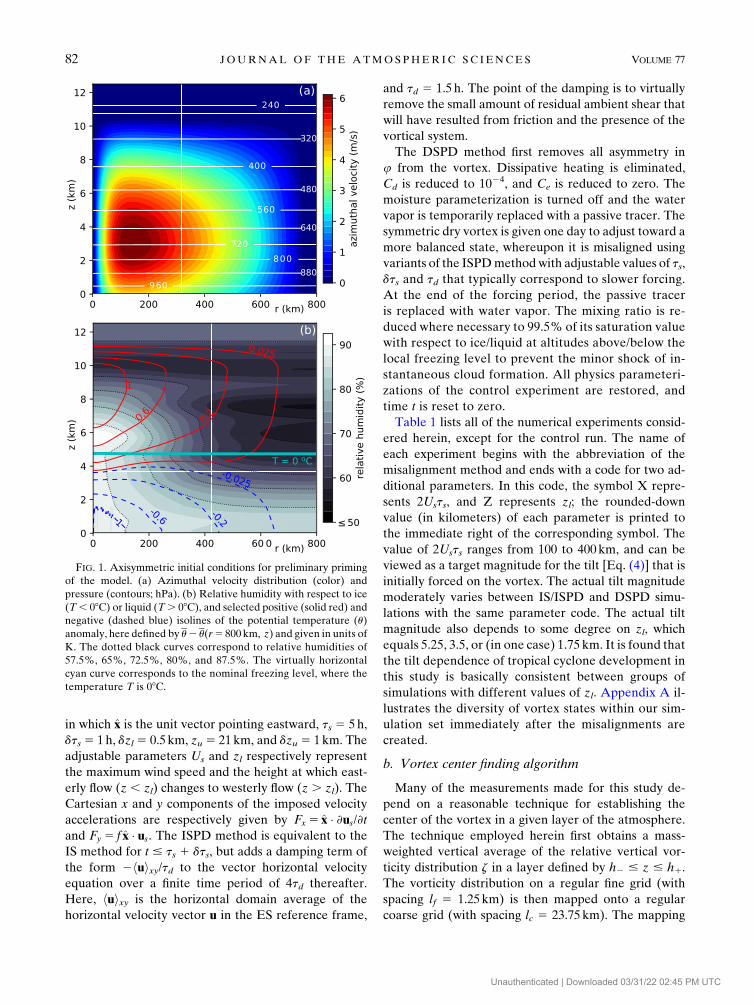
RHd. Figure 1 depicts both the primary circulation

and the moist thermodynamic structure of the initial

condition.

The misalignment experiments are initialized with

conditions derived from the control simulation 99h into

its development, shortly before one might declare the

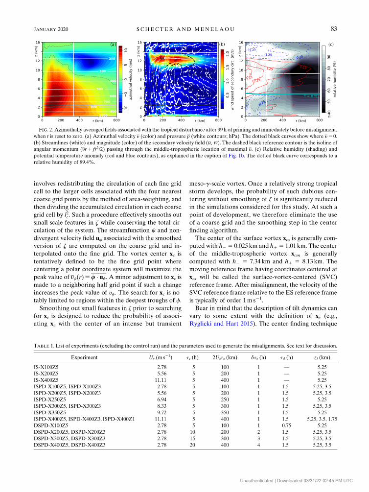
genesis of a warm core tropical cyclone. Figure 2 depicts

the azimuthally averaged fluid variables at this time,

henceforth labeled t 5 0. The absolute maximum of y

occurring at r 5 115.1 km and z 5 3.7 km is 12.0m s21;

the surface maximum is 8.6m s21 at r 5 42.9 km. An

upper-tropospheric anticyclone (Fig. 2a) has emerged in

the outflow of a weak secondary circulation (Fig. 2b).

Furthermore, the relative humidity has broadly in-

tensified throughout the central region of the vortex

(Fig. 2c).

In each experiment, the misalignment is created using

one of the following three techniques: impulsive sepa-

ration (IS), impulsive separation plus damping (ISPD),

and dry separation plus damping (DSPD). The IS

method introduces forcing terms to the horizontal ve-

locity equations that—in a frictionless quiescent atmo-

sphere—would generate a transient shear flow in the

Earth-stationary (ES) reference frame of the following

form:

us(z, t)5 x

Us

2tanh

�z2 z

l

dzl

��1:01 tanh

�zu2 z

dzu

��

3

8>>>>>><>>>>>>:

t/dts, t, dt

s

1, dts# t# t

s

12 (t2 ts)/dt

s, t

s, t, t

s1 dt

s

0, t$ ts1 dt

s

, (3)



in which x is the unit vector pointing eastward, ts 5 5 h,

dts 5 1 h, dzl 5 0.5 km, zu 5 21km, and dzu 5 1km. The

adjustable parameters Us and zl respectively represent

the maximum wind speed and the height at which east-

erly flow (z , zl) changes to westerly flow (z . zl). The

Cartesian x and y components of the imposed velocity

accelerations are respectively given by Fx 5 x � ›us/›t

and Fy 5 f x � us. The ISPD method is equivalent to the

IS method for t # ts 1 dts, but adds a damping term of

the form 2huixy/td to the vector horizontal velocity

equation over a finite time period of 4td thereafter.

Here, huixy is the horizontal domain average of the

horizontal velocity vector u in the ES reference frame,

and td 5 1.5 h. The point of the damping is to virtually

remove the small amount of residual ambient shear that

will have resulted from friction and the presence of the

vortical system.

The DSPD method first removes all asymmetry in

u from the vortex. Dissipative heating is eliminated,

Cd is reduced to 1024, and Ce is reduced to zero. The

moisture parameterization is turned off and the water

vapor is temporarily replaced with a passive tracer. The

symmetric dry vortex is given one day to adjust toward a

more balanced state, whereupon it is misaligned using

variants of the ISPDmethodwith adjustable values of ts,

dts and td that typically correspond to slower forcing.

At the end of the forcing period, the passive tracer

is replaced with water vapor. The mixing ratio is re-

duced where necessary to 99.5% of its saturation value

with respect to ice/liquid at altitudes above/below the

local freezing level to prevent the minor shock of in-

stantaneous cloud formation. All physics parameteri-

zations of the control experiment are restored, and

time t is reset to zero.

Table 1 lists all of the numerical experiments consid-

ered herein, except for the control run. The name of

each experiment begins with the abbreviation of the

misalignment method and ends with a code for two ad-

ditional parameters. In this code, the symbol X repre-

sents 2Usts, and Z represents zl; the rounded-down

value (in kilometers) of each parameter is printed to

the immediate right of the corresponding symbol. The

value of 2Usts ranges from 100 to 400km, and can be

viewed as a target magnitude for the tilt [Eq. (4)] that is

initially forced on the vortex. The actual tilt magnitude

moderately varies between IS/ISPD and DSPD simu-

lations with the same parameter code. The actual tilt

magnitude also depends to some degree on zl, which

equals 5.25, 3.5, or (in one case) 1.75 km. It is found that

the tilt dependence of tropical cyclone development in

this study is basically consistent between groups of

simulations with different values of zl. Appendix A il-

lustrates the diversity of vortex states within our sim-

ulation set immediately after the misalignments are

created.

b. Vortex center finding algorithm

Many of the measurements made for this study de-

pend on a reasonable technique for establishing the

center of the vortex in a given layer of the atmosphere.

The technique employed herein first obtains a mass-

weighted vertical average of the relative vertical vor-

ticity distribution z in a layer defined by h2 # z # h1.

The vorticity distribution on a regular fine grid (with

spacing lf 5 1.25 km) is then mapped onto a regular

coarse grid (with spacing lc 5 23.75 km). The mapping

FIG. 1. Axisymmetric initial conditions for preliminary priming

of the model. (a) Azimuthal velocity distribution (color) and

pressure (contours; hPa). (b) Relative humidity with respect to ice

(T, 08C) or liquid (T. 08C), and selected positive (solid red) and

negative (dashed blue) isolines of the potential temperature (u)

anomaly, here defined by u2 u(r5 800 km, z) and given in units of

K. The dotted black curves correspond to relative humidities of

57.5%, 65%, 72.5%, 80%, and 87.5%. The virtually horizontal

cyan curve corresponds to the nominal freezing level, where the

temperature T is 08C.



involves redistributing the circulation of each fine grid

cell to the larger cells associated with the four nearest

coarse grid points by the method of area-weighting, and

then dividing the accumulated circulation in each coarse

grid cell by l2c . Such a procedure effectively smooths out

small-scale features in z while conserving the total cir-

culation of the system. The streamfunction c and non-

divergent velocity field uc associated with the smoothed

version of z are computed on the coarse grid and in-

terpolated onto the fine grid. The vortex center xc is

tentatively defined to be the fine grid point where

centering a polar coordinate system will maximize the

peak value of yc(r)[ u � uc. A minor adjustment to xc is

made to a neighboring half grid point if such a change

increases the peak value of yc. The search for xc is no-

tably limited to regions within the deepest troughs of c.

Smoothing out small features in z prior to searching

for xc is designed to reduce the probability of associ-

ating xc with the center of an intense but transient

meso-g-scale vortex. Once a relatively strong tropical

storm develops, the probability of such dubious cen-

tering without smoothing of z is significantly reduced

in the simulations considered for this study. At such a

point of development, we therefore eliminate the use

of a coarse grid and the smoothing step in the center

finding algorithm.

The center of the surface vortex xcs is generally com-

puted with h2 5 0.025 km and h1 5 1.01 km. The center

of the middle-tropospheric vortex xcm is generally

computed with h2 5 7.34 km and h1 5 8.13 km. The

moving reference frame having coordinates centered at

xcs will be called the surface-vortex-centered (SVC)

reference frame. After misalignment, the velocity of the

SVC reference frame relative to the ES reference frame

is typically of order 1ms21.

Bear in mind that the description of tilt dynamics can

vary to some extent with the definition of xc (e.g.,

Ryglicki and Hart 2015). The center finding technique

TABLE 1. List of experiments (excluding the control run) and the parameters used to generate the misalignments. See text for discussion.

Experiment Us (m s21) ts (h) 2Usts (km) dts (h) td (h) zl (km)

IS-X100Z5 2.78 5 100 1 — 5.25

IS-X200Z5 5.56 5 200 1 — 5.25

IS-X400Z5 11.11 5 400 1 — 5.25

ISPD-X100Z5, ISPD-X100Z3 2.78 5 100 1 1.5 5.25, 3.5

ISPD-X200Z5, ISPD-X200Z3 5.56 5 200 1 1.5 5.25, 3.5

ISPD-X250Z5 6.94 5 250 1 1.5 5.25

ISPD-X300Z5, ISPD-X300Z3 8.33 5 300 1 1.5 5.25, 3.5

ISPD-X350Z5 9.72 5 350 1 1.5 5.25

ISPD-X400Z5, ISPD-X400Z3, ISPD-X400Z1 11.11 5 400 1 1.5 5.25, 3.5, 1.75

DSPD-X100Z5 2.78 5 100 1 0.75 5.25

DSPD-X200Z5, DSPD-X200Z3 2.78 10 200 2 1.5 5.25, 3.5

DSPD-X300Z5, DSPD-X300Z3 2.78 15 300 3 1.5 5.25, 3.5

DSPD-X400Z5, DSPD-X400Z3 2.78 20 400 4 1.5 5.25, 3.5

FIG. 2. Azimuthally averaged fields associated with the tropical disturbance after 99 h of priming and immediately beforemisalignment,

when t is reset to zero. (a) Azimuthal velocity y (color) and pressure p (white contours; hPa). The dotted black curves show where y5 0.

(b) Streamlines (white) and magnitude (color) of the secondary velocity field (u, w). The dashed black reference contour is the isoline of

angular momentum (yr1 fr2/2) passing through the middle-tropospheric location of maximal y. (c) Relative humidity (shading) and

potential temperature anomaly (red and blue contours), as explained in the caption of Fig. 1b. The dotted black curve corresponds to a

relative humidity of 89.4%.



described above is presently favored by the authors and

(in essence) within the domain of conventional practice.

For those interested, appendix B briefly addresses the

consequences of using an alternative technique; the con-

tents of this appendix are best read after section 4a.

3. Impact of misalignment on hurricane formation

a. Hindered intensification of the maximum surfacewind speed

The central issue considered in this section of the ar-

ticle is the effect of misalignment on the time required

for the surface vortex to intensify. The misalignment is

quantified by the following tilt vector:

Dxc[ x

cm2 x

cs. (4)

By definition, Dxc gives the magnitude and direction of

the horizontal displacement of the rotational center of

the middle-tropospheric vortex from its counterpart at the

surface. Our primary measure of tropical cyclone

intensity is the maximum value of the azimuthally

averaged tangential velocity at the lowest grid level

above the ocean, denoted by ym. Needless to say, the

pertinent value of ym is that measured in the SVC

coordinate system.

Let tITC denote the time during the evolution of an

incipient tropical cyclone (ITC) when ym first reaches a

modest pre–tropical storm value of 12.5m s21. Further-

more, let tCAT1 denote the time when ym first reaches a

value of 32.5m s21, which approximately corresponds

to the threshold wind speed of a category-1 (CAT1)

hurricane. Henceforth, the time interval between the

aforementioned events will be called the hurricane for-

mation period (HFP). The duration of the HFP is given

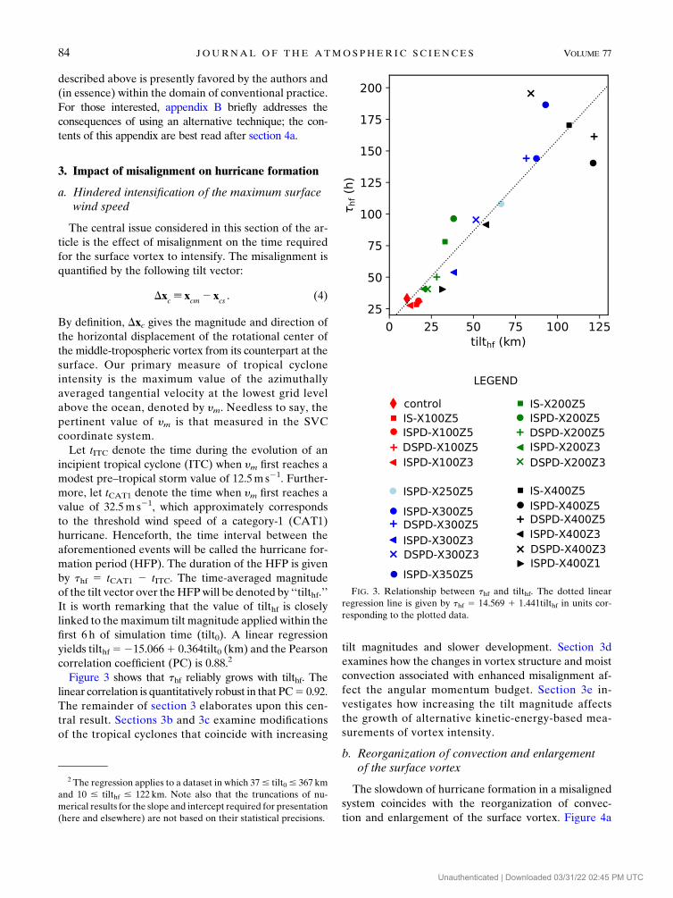
by thf 5 tCAT1 2 tITC. The time-averaged magnitude

of the tilt vector over theHFPwill be denoted by ‘‘tilthf.’’

It is worth remarking that the value of tilthf is closely

linked to themaximum tilt magnitude applied within the

first 6 h of simulation time (tilt0). A linear regression

yields tilthf5215.0661 0.364tilt0 (km) and the Pearson

correlation coefficient (PC) is 0.88.2

Figure 3 shows that thf reliably grows with tilthf. The

linear correlation is quantitatively robust in that PC5 0.92.

The remainder of section 3 elaborates upon this cen-

tral result. Sections 3b and 3c examine modifications

of the tropical cyclones that coincide with increasing

tilt magnitudes and slower development. Section 3d

examines how the changes in vortex structure and moist

convection associated with enhanced misalignment af-

fect the angular momentum budget. Section 3e in-

vestigates how increasing the tilt magnitude affects

the growth of alternative kinetic-energy-based mea-

surements of vortex intensity.

b. Reorganization of convection and enlargementof the surface vortex

The slowdown of hurricane formation in a misaligned

system coincides with the reorganization of convec-

tion and enlargement of the surface vortex. Figure 4a

FIG. 3. Relationship between thf and tilthf. The dotted linear

regression line is given by thf 5 14.569 1 1.441tilthf in units cor-

responding to the plotted data.

2 The regression applies to a dataset in which 37# tilt0# 367 km

and 10 # tilthf # 122 km. Note also that the truncations of nu-

merical results for the slope and intercept required for presentation

(here and elsewhere) are not based on their statistical precisions.



demonstrates that greater values of tilthf correspond to

greater values of the time-averaged precipitation radius

rp. By definition, rp is the radius in the SVC coordinate

system at which the azimuthally averaged 2-h pre-

cipitation (surface rainfall) distribution is maximized.

Figure 4b shows that the time average of the radius rm at

which ym occurs grows commensurately with rp.

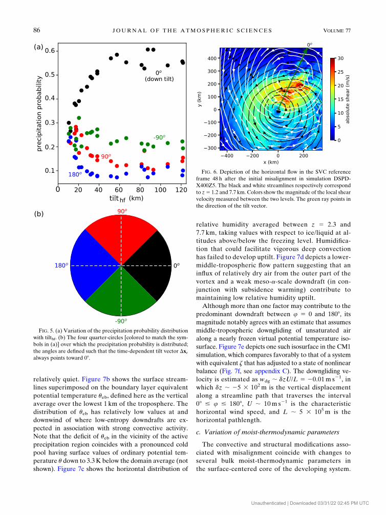
In addition to moving outward, the precipitation

grows increasingly asymmetric with enhanced tilt.

Figure 5 depicts the tilthf dependence of the 2-h pre-

cipitation asymmetry during the HFP. The total (area

integrated) 2-h precipitation in a 400-km circular disc

centered at xcs is split into individual contributions

from 4 quarter circles. The quarter circles are centered

in azimuth at u 5 08, 908, 1808, and 2708 (2908), withu5 0 corresponding to the downtilt direction (i.e., the

direction of Dxc). Each absolute contribution to the

2-h precipitation is then divided by the total to form

a fractional contribution. The plotted precipitation

probability is the time average of the fractional contri-

bution over the HFP. As tilthf increases from 10 to

60 km, the probability of precipitation in the downtilt

quadrant dramatically grows from slightly above 25% to

approximately 60%. The probability of precipitation in

the uptilt quadrant (centered at 1808) decays to a value

substantially less than 10%. The precipitation proba-

bilities in the quadrants centered at 2908 and 908 alsodiminish, but the former decays less than the latter.

For illustrative purposes, Figs. 6 and 7 depict the

asymmetric structure of the vortex in simulation DSPD-

X400Z5 at a time during the HFP when jDxcj5 240 km.

DSPD-X400Z5 is among a handful of simulations most

worthy (in our view) of detailed examination, because

the misalignment coincides with severely hindered de-

velopment of the tropical cyclone. The structure of the

vortex in DSPD-X400Z5 is similar to that found in

earlier studies of real-world and simulated tropical cy-

clones that are tilted by moderate environmental wind

shear prior to achieving hurricane status (e.g., Rappin

and Nolan 2012; Nguyen et al. 2017). Figure 6 shows the

misalignment of quasi-circular lower-tropospheric (lw)

and middle-tropospheric (md) streamlines in the slowly

moving SVC reference frame, superimposed on a com-

plementary plot of the magnitude of the local shear

velocity, defined by umd 2 ulw.3 The lower- and middle-

tropospheric flows specifically correspond to elevations of

1.2 and 7.7km above sea level. The green ray represents

the u 5 0 axis and therefore points exactly downtilt.

Figure 7a shows the 2-h precipitation field rotated

such that downtilt is now directly to the right. Con-

sistent with Fig. 5, much of the precipitation is seen in

the downtilt quadrant, whereas the uptilt quadrant is

FIG. 4. (a) Precipitation radius rp averaged over the HFP vs tilthf.

The dotted linear regression line is given by rp 5 18.8251 0.775tilthf(km) and the correlation coefficient is 0.96. (b)Relationship between

rp and the radius of maximum surface-y, denoted rm, averaged over

theHFP. The dotted reference line corresponds to rp5 rm. See Fig. 3

for the symbol legend.

3 A qualitatively similar shear pattern but with a smaller maxi-

mummagnitude of 22m s21 (19m s21) is seenwhen umd and ulw are

first smoothed using a Gaussian kernel with a standard deviation of

30 km (60 km) in both x and y. A similar pattern is also seen at t5 0,

prior to any convection in experiment DSPD-X400Z5, but with a

peak shearmagnitude of 14m s21 more directly between the lower-

and middle-tropospheric centers of rotation.



relatively quiet. Figure 7b shows the surface stream-

lines superimposed on the boundary layer equivalent

potential temperature ueb, defined here as the vertical

average over the lowest 1 km of the troposphere. The

distribution of ueb has relatively low values at and

downwind of where low-entropy downdrafts are ex-

pected in association with strong convective activity.

Note that the deficit of ueb in the vicinity of the active

precipitation region coincides with a pronounced cold

pool having surface values of ordinary potential tem-

perature u down to 3.3K below the domain average (not

shown). Figure 7c shows the horizontal distribution of

relative humidity averaged between z 5 2.3 and

7.7 km, taking values with respect to ice/liquid at al-

titudes above/below the freezing level. Humidifica-

tion that could facilitate vigorous deep convection

has failed to develop uptilt. Figure 7d depicts a lower-

middle-tropospheric flow pattern suggesting that an

influx of relatively dry air from the outer part of the

vortex and a weak meso-a-scale downdraft (in con-

junction with subsidence warming) contribute to

maintaining low relative humidity uptilt.

Although more than one factor may contribute to the

predominant downdraft between u 5 0 and 1808, itsmagnitude notably agrees with an estimate that assumes

middle-tropospheric downgliding of unsaturated air

along a nearly frozen virtual potential temperature iso-

surface. Figure 7e depicts one such isosurface in the CM1

simulation, which compares favorably to that of a system

with equivalent z that has adjusted to a state of nonlinear

balance (Fig. 7f, see appendix C). The downgliding ve-

locity is estimated as wdg ; dzU/L 5 20.01m s21, in

which dz ; 25 3 102m is the vertical displacement

along a streamline path that traverses the interval

08 # u # 1808, U ; 10m s21 is the characteristic

horizontal wind speed, and L ; 5 3 105m is the

horizontal pathlength.

c. Variation of moist-thermodynamic parameters

The convective and structural modifications asso-

ciated with misalignment coincide with changes to

several bulk moist-thermodynamic parameters in

the surface-centered core of the developing system.

FIG. 6. Depiction of the horizontal flow in the SVC reference

frame 48 h after the initial misalignment in simulation DSPD-

X400Z5. The black and white streamlines respectively correspond

to z5 1.2 and 7.7 km. Colors show the magnitude of the local shear

velocity measured between the two levels. The green ray points in

the direction of the tilt vector.

FIG. 5. (a) Variation of the precipitation probability distribution

with tilthf. (b) The four quarter-circles [colored to match the sym-

bols in (a)] over which the precipitation probability is distributed;

the angles are defined such that the time-dependent tilt vector Dxcalways points toward 08.



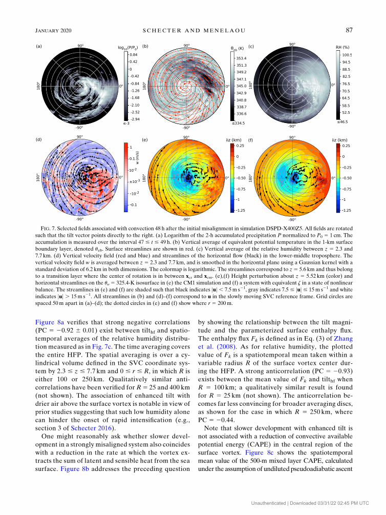
Figure 8a verifies that strong negative correlations

(PC 5 20.92 6 0.01) exist between tilthf and spatio-

temporal averages of the relative humidity distribu-

tion measured as in Fig. 7c. The time averaging covers

the entire HFP. The spatial averaging is over a cy-

lindrical volume defined in the SVC coordinate sys-

tem by 2.3 # z # 7.7 km and 0 # r # R, in which R is

either 100 or 250 km. Qualitatively similar anti-

correlations have been verified for R5 25 and 400 km

(not shown). The association of enhanced tilt with

drier air above the surface vortex is notable in view of

prior studies suggesting that such low humidity alone

can hinder the onset of rapid intensification (e.g.,

section 3 of Schecter 2016).

One might reasonably ask whether slower devel-

opment in a strongly misaligned system also coincides

with a reduction in the rate at which the vortex ex-

tracts the sum of latent and sensible heat from the sea

surface. Figure 8b addresses the preceding question

by showing the relationship between the tilt magni-

tude and the parameterized surface enthalpy flux.

The enthalpy flux Fk is defined as in Eq. (3) of Zhang

et al. (2008). As for relative humidity, the plotted

value of Fk is a spatiotemporal mean taken within a

variable radius R of the surface vortex center dur-

ing the HFP. A strong anticorrelation (PC 5 20.93)

exists between the mean value of Fk and tilthf when

R 5 100 km; a qualitatively similar result is found

for R 5 25 km (not shown). The anticorrelation be-

comes far less convincing for broader averaging discs,

as shown for the case in which R 5 250 km, where

PC 5 20.44.

Note that slower development with enhanced tilt is

not associated with a reduction of convective available

potential energy (CAPE) in the central region of the

surface vortex. Figure 8c shows the spatiotemporal

mean value of the 500-m mixed layer CAPE, calculated

under the assumption of undiluted pseudoadiabatic ascent

FIG. 7. Selected fields associated with convection 48 h after the initial misalignment in simulation DSPD-X400Z5. All fields are rotated

such that the tilt vector points directly to the right. (a) Logarithm of the 2-h accumulated precipitation P normalized to P0 5 1 cm. The

accumulation is measured over the interval 47 # t # 49 h. (b) Vertical average of equivalent potential temperature in the 1-km surface

boundary layer, denoted ueb. Surface streamlines are shown in red. (c) Vertical average of the relative humidity between z 5 2.3 and

7.7 km. (d) Vertical velocity field (red and blue) and streamlines of the horizontal flow (black) in the lower-middle troposphere. The

vertical velocity field w is averaged between z 5 2.3 and 7.7 km, and is smoothed in the horizontal plane using a Gaussian kernel with a

standard deviation of 6.2 km in both dimensions. The colormap is logarithmic. The streamlines correspond to z5 5.6 km and thus belong

to a transition layer where the center of rotation is in between xcs and xcm. (e),(f) Height perturbation about z 5 5.52 km (color) and

horizontal streamlines on the uy 5 325.4-K isosurface in (e) the CM1 simulation and (f) a system with equivalent z in a state of nonlinear

balance. The streamlines in (e) and (f) are shaded such that black indicates juj, 7.5m s21, gray indicates 7.5 # juj# 15m s21 and white

indicates juj . 15m s21. All streamlines in (b) and (d)–(f) correspond to u in the slowly moving SVC reference frame. Grid circles are

spaced 50m apart in (a)–(d); the dotted circles in (e) and (f) show where r 5 200m.



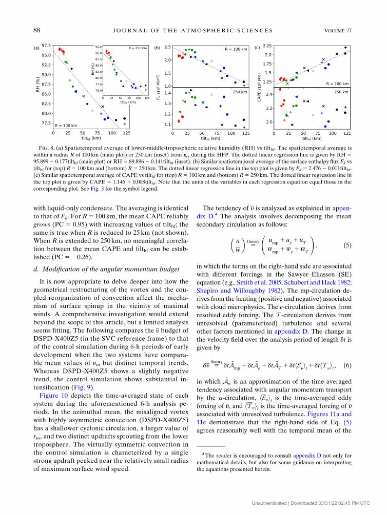
with liquid-only condensate. The averaging is identical

to that of Fk. For R5 100 km, the mean CAPE reliably

grows (PC 5 0.95) with increasing values of tilthf; the

same is true when R is reduced to 25 km (not shown).

When R is extended to 250 km, no meaningful correla-

tion between the mean CAPE and tilthf can be estab-

lished (PC 5 20.26).

d. Modification of the angular momentum budget

It is now appropriate to delve deeper into how the

geometrical restructuring of the vortex and the cou-

pled reorganization of convection affect the mecha-

nism of surface spinup in the vicinity of maximal

winds. A comprehensive investigation would extend

beyond the scope of this article, but a limited analysis

seems fitting. The following compares the y budget of

DSPD-X400Z5 (in the SVC reference frame) to that

of the control simulation during 6-h periods of early

development when the two systems have compara-

ble mean values of ym but distinct temporal trends.

Whereas DSPD-X400Z5 shows a slightly negative

trend, the control simulation shows substantial in-

tensification (Fig. 9).

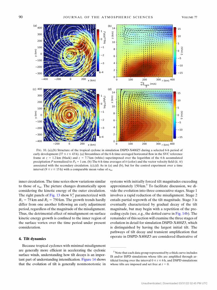
Figure 10 depicts the time-averaged state of each

system during the aforementioned 6-h analysis pe-

riods. In the azimuthal mean, the misaligned vortex

with highly asymmetric convection (DSPD-X400Z5)

has a shallower cyclonic circulation, a larger value of

rm, and two distinct updrafts sprouting from the lower

troposphere. The virtually symmetric convection in

the control simulation is characterized by a single

strong updraft peaked near the relatively small radius

of maximum surface wind speed.

The tendency of y is analyzed as explained in appen-

dix D.4 The analysis involves decomposing the mean

secondary circulation as follows:

�u

w

�5

theory

ump

1 ue1 uT

wmp

1we1wT

!, (5)

in which the terms on the right-hand side are associated

with different forcings in the Sawyer–Eliassen (SE)

equation (e.g., Smith et al. 2005; Schubert andHack 1982;

Shapiro and Willoughby 1982). The mp-circulation de-

rives from the heating (positive and negative) associated

with cloud microphysics. The e-circulation derives from

resolved eddy forcing. The T -circulation derives from

unresolved (parameterized) turbulence and several

other factors mentioned in appendix D. The change in

the velocity field over the analysis period of length dt is

given by

dy 5theory

dt ~Amp

1 dt ~Ae1 dt ~AT 1 dthE

yit1 dthT

yit, (6)

in which ~Aa is an approximation of the time-averaged

tendency associated with angular momentum transport

by the a-circulation, hEyit is the time-averaged eddy

forcing of y, and hT yit is the time-averaged forcing of y

associated with unresolved turbulence. Figures 11a and

11c demonstrate that the right-hand side of Eq. (5)

agrees reasonably well with the temporal mean of the

FIG. 8. (a) Spatiotemporal average of lower-middle-tropospheric relative humidity (RH) vs tilthf. The spatiotemporal average is

within a radius R of 100 km (main plot) or 250 km (inset) from xcs during the HFP. The dotted linear regression line is given by RH 595.8992 0.177tilthf (main plot) or RH5 89.8962 0.141tilthf (inset). (b) Similar spatiotemporal average of the surface enthalpy flux Fk vs

tilthf for (top) R5 100 km and (bottom) R5 250 km. The dotted linear regression line in the top plot is given by Fk 5 2.4762 0.011tilthf.

(c) Similar spatiotemporal average of CAPE vs tilthf for (top) R5 100 km and (bottom) R5 250 km. The dotted linear regression line in

the top plot is given by CAPE 5 1.146 1 0.008tilthf. Note that the units of the variables in each regression equation equal those in the

corresponding plot. See Fig. 3 for the symbol legend.

4 The reader is encouraged to consult appendix D not only for

mathematical details, but also for some guidance on interpreting

the equations presented herein.



actual secondary circulation in both CM1 simulations

under present consideration. Figures 11b and 11d fur-

thermore validate Eq. (6).

Figures 12a–d show the individual contributions to dy

[Eq. (6)] in simulation DSPD-X400Z5. It is seen that the

mp-circulation acts to broadly accelerate the cyclonic

winds in the lower troposphere. If acting alone, the mp-

circulation would boost the near-surface values of y by

up to 5ms21 in the neighborhood of the maximal winds

of the time-averaged vortex. Of course, other factors are

equally important to the azimuthal velocity budget.

Stronger positive and negative tendencies are found

near the surface in association with the T -circulation

and direct forcing by unresolved turbulent transport;

their combination (not shown) is predominantly nega-

tive. The tendencies associated with the e-circulation

and direct eddy forcing near the maximal surface winds

are smaller but relevant.

Figures 12e–h show the contributions to dy in the

control simulation.Here one finds that themp-circulation

more vigorously accelerates the cyclonic winds of the

inner core. If left uncontested, the mp-circulation would

boost the near surface values of y by 9–10ms21 slightly

outward of the maximal winds of the time-averaged vor-

tex. The positive and negative contributions from dt ~ATand dthT yit near the surface are qualitatively similar to

their counterparts in themisaligned system, and are again

net-negative (not shown) in the vicinity of maximal y.

In the same region, dt ~Ae and dthEyit are appreciable

but mutually opposing.

Perhaps the main result from the foregoing analysis is

that the restructuring of the vortex and the re-

organization of convection in the misaligned system

rendered the mp-circulation less effective in accelerat-

ing the maximum of y near the sea surface. In the case at

hand, such reduced efficiency allowed the net negative

contribution from other factors in the azimuthal velocity

budget (which stayed sufficiently strong) to completely

nullify the growth of ym.

Note that reasonable accuracy of the SE-based anal-

ysis relied partly on the small fractional difference (0.3

or less) between the gradient wind and y in the vicinity of

the surface maximum. The error may worsen consider-

ably at a later stage of development if the degree of

gradient imbalance were to intensify in the boundary

layer, as often occurs in simulations of tropical cyclones

(e.g., Bui et al. 2009; Montgomery and Smith 2014;

Schecter 2016). In an alternative experiment where tilt is

introduced at such a time, the detrimental effect of the

associated convective asymmetry on intensification of

ymmight be compounded by limiting supergradient flow

(cf. Schecter 2013). A separate study would be required

to shed light on this issue.

e. Surface kinetic energy growth

One might wonder whether increasing the tilt mag-

nitude has the same qualitative effect on all measures

of vortex intensity. Herein, we address the preceding

question by comparing time series of several intensity

parameters. Figure 13 (left) shows the temporal

growth of ym for all simulations over the time scale for

the virtually aligned control vortex to mature into a

well-developed hurricane. Each thick curve covers

the spread in a group of vortices that are initially

perturbed with similar target misalignments (2Usts)

and equivalent values of zl. Consistent with Fig. 3, the

time series exhibit considerable variation; enhanced

tilt markedly slows the intensification of ym.

Alternatively, one might consider the temporal am-

plification of kinetic energy. Neglecting minor density

variations, the kinetic energy contained in the primary

component of the surface circulation over the interval

R1 # r # R2 is directly proportional to

V2s [

2

R22 2R2

1

ðR2

R1

drry2s , (7)

in which ys denotes y measured in the SVC coordinate

system at the first grid level above the ocean. The center

panels of Fig. 13 showV2s parameterized withR15 0 and

R2 5 75 km, so as to represent the kinetic energy of the

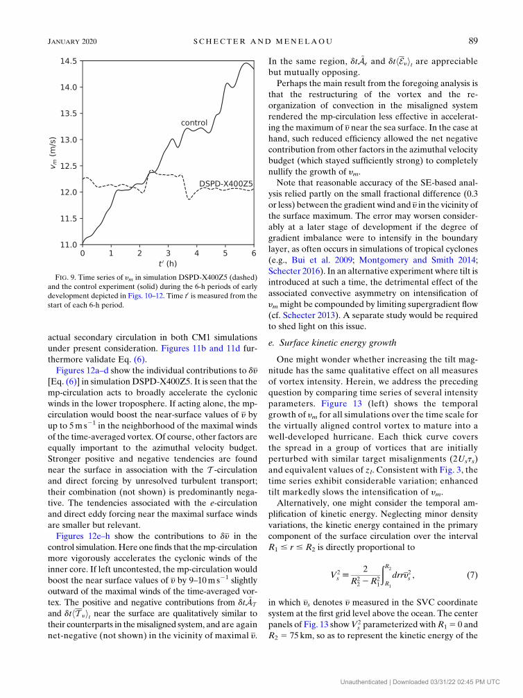
FIG. 9. Time series of ym in simulation DSPD-X400Z5 (dashed)

and the control experiment (solid) during the 6-h periods of early

development depicted in Figs. 10–12. Time t0 is measured from the

start of each 6-h period.



inner circulation. The time series show variations similar

to those of ym. The picture changes dramatically upon

considering the kinetic energy of the outer circulation.

The right panels of Fig. 13 show V2s parameterized with

R1 5 75km and R2 5 750km. The growth trends hardly

differ from one another following an early adjustment

period, regardless of themagnitude of themisalignment.

Thus, the detrimental effect of misalignment on surface

kinetic energy growth is confined to the inner region of

the surface vortex over the time period under present

consideration.

4. Tilt dynamics

Because tropical cyclones with minimal misalignment

are generally more efficient in accelerating the cyclonic

surface winds, understanding how tilt decays is an impor-

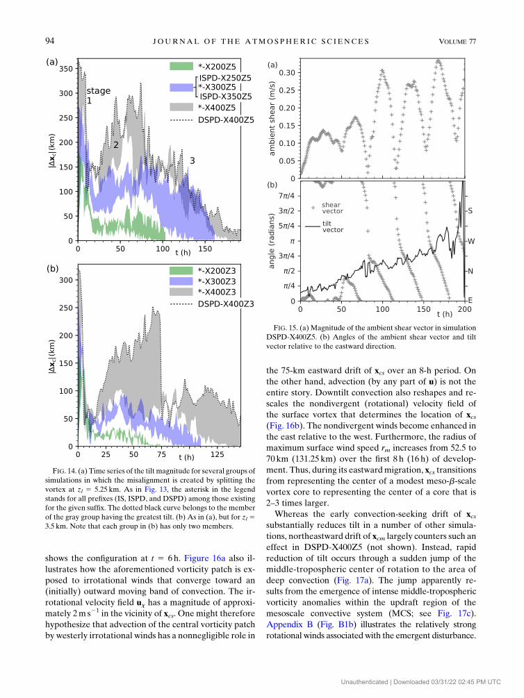
tant part of understanding intensification. Figure 14 shows

that the evolution of tilt is generally nonmonotonic in

systems with initially forced tilt magnitudes exceeding

approximately 150 km.5 To facilitate discussion, we di-

vide the evolution into three consecutive stages. Stage 1

involves a rapid reduction of the misalignment. Stage 2

entails partial regrowth of the tilt magnitude. Stage 3 is

eventually characterized by gradual decay of the tilt

magnitude, but may begin with a repetition of the pre-

ceding cycle (see, e.g., the dotted curve in Fig. 14b). The

remainder of this section will examine the three stages of

evolution in detail for simulation DSPD-X400Z5, which

is distinguished by having the largest initial tilt. The

pathways of tilt decay and transient amplification that

operate in DSPD-X400Z5 are considered illustrative of

FIG. 10. (a),(b) Structure of the tropical cyclone in simulation DSPD-X400Z5 during a selected 6-h period of

early development (37 # t # 43 h). (a) Streamlines of the 6-h time-averaged horizontal flow in the SVC reference

frame at z 5 1.2 km (black) and z 5 7.7 km (white) superimposed over the logarithm of the 6-h accumulated

precipitation P normalized to P0 5 1 cm. (b) The 6-h time averages of y (color) and the vector velocity field (u, w)

associated with the secondary circulation. (c),(d) As in (a) and (b), but for the control experiment over a time

interval (9 # t # 15 h) with a comparable mean value of ym.

5 Note that each data group represented by a thick curve includes

IS and/or ISPD simulations whose tilts are amplified through ar-

tificial forcing over the interval 0# t# 6 h, and DSPD simulations

whose tilts are imposed and set free at t 5 0.



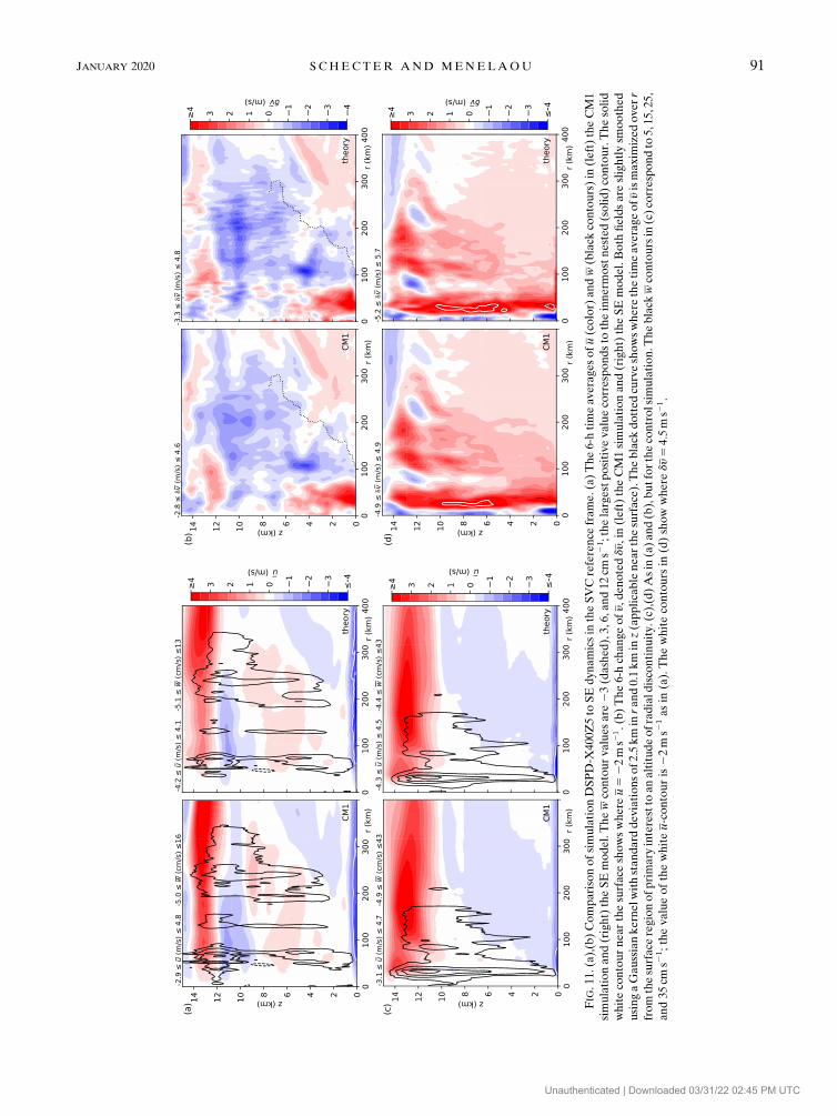
FIG.11.(a),(b)ComparisonofsimulationDSPD-X

400Z5to

SEdynamicsin

theSVCreference

frame.(a)The6-h

timeaveragesofu(color)andw(black

contours)in

(left)theCM1

simulationand(right)theSEmodel.Thewcontourvaluesare

23(dashed

),3,6,and12cm

s21;thelargestpositivevaluecorrespondsto

theinnerm

ostnested(solid)contour.Thesolid

whitecontournear

thesurfaceshowswhere

u522ms2

1.(b)The6-h

changeofy,denoteddy,in

(left)theCM1simulationand(right)theSEmodel.Both

fieldsare

slightlysm

oothed

usingaGaussiankernelw

ithstandard

deviationsof2.5km

inrand0.1km

inz(applicablenear

thesurface).Theblack

dottedcurveshowswhere

thetimeaverageofyismaxim

ized

over

r

from

thesurface

regionofprimary

interestto

analtitudeofradiald

iscontinuity.(c),(d)Asin

(a)and(b),butforthecontrolsim

ulation.T

heblack

wcontoursin

(c)correspondto

5,15,25,

and35cm

s21;thevalueofthewhiteu-contouris22m

s21asin

(a).Thewhitecontours

in(d)show

where

dy54:5ms2

1.



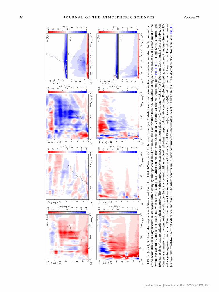
FIG.12.(a)–(d)SE-baseddecompositionofdyin

simulationDSPD-X

400Z5in

theSVCreference

frame.(a)Contributionfrom

theadvectionofangularmomen

tum

bythecomponent

ofthesymmetricsecondary

circulationassociatedwithheatingbymicrophysicalcloudprocesses.(b)Contributionfrom

theadvectionofangularmomen

tum

bythecomponentofthe

symmetricsecondary

circulationassociatedwithresolvededdies.(c)Direct

contributionfrom

resolvededdyforcing,withslightsm

oothingasin

Fig.11b.(d)(top)Directcontribution

from

unresolved(parameterized)turbulenttransport.T

hewhitecontourshaveouterm

ost-to-innerm

ostvaluesof27,2

10,and213m

s21.(d)(bottom)Contributionfrom

theadvection

ofangularmomen

tum

bythesymmetricsecondary

circulationassociatedwithunresolvedturbulenttransport,dissipativeheating,R

ayleighdamping,andaminorutendency

linkedto

3D

velocity-divergence

inmoistair.Thewhitecontours

haveouterm

ost-to-innerm

ostvaluesof7and10m

s21.(e)–(h)Asin

(a)–(d),butforthecontrolsimulation.Thewhitecontours

in

(e)have

outerm

ost-to-innerm

ostvalues

of6and9m

s21.T

hewhitecontoursin

(h)have

outerm

ost-to-innerm

ostvalues

of68and616m

s21.T

hedottedblack

contoursare

asin

Fig.11.



many (but not all) of the possibilities. Some of the

known similarities and differences with other simula-

tions will be noted as the narrative proceeds.

Before discussing the intricacies of tilt evolution in

DSPD-X400Z5, it is worthwhile to briefly consider the

potential relevance of ambient wind shear that may arise

over time despite our elimination of the extraneous

forcing that created the initial misalignment. Figure 15

shows time series of the magnitude and angle of the

ambient shear vector, defined by hum 2 usixy, in which

um (us) is the vertically averaged horizontal velocity

in the middle-tropospheric (near-surface) layer corre-

sponding to where xcm (xcs) is measured. It is found that

the shear magnitude remains weak (0–0.35ms21) and

undulates over the course of the simulation (Fig. 15a).

Ambient wind shear possessing one-half the maximum

intensity seen here—acting in a direction parallel (an-

tiparallel) to the tilt vector—would amplify (diminish)

the tilt of the tropical cyclone at a rate of 15 kmday21.

Such a rate is too small to account for the tilt tenden-

cies found at any stage of evolution. Moreover, during

the final and slowest stage of alignment, the shear

vector rotates anticyclonically on a time scale that is

short (an inertial period) compared to the precession

period of the tilt vector (Fig. 15b). It follows that ex-

trinsic forcing by ambient shear is not only weak but

inefficient.

a. Stage 1

The first stage of tilt evolution is characterized by

rapid decay of the measured misalignment. Such decay

commonly coincides with the migration of xcs toward an

area of vigorous deep cumulus convection in the general

direction of xcm. Figure 16 provides a minimal depiction

of the process during the first 8 h of simulation DSPD-

X400Z5. At any arbitrary instant during this 8-h period,

the surface center of rotation sits roughly in the middle

of a 100-km scale patch of cyclonic vorticity. Figure 16a

FIG. 13. (a) Time series of the (left) maximum and (center, right) mean-squared values of the azimuthally averaged tangential velocity

field (in the SVC coordinate system) at the sea surface for several groups of simulations in which the misalignment is created by splitting

the vortex at zl 5 5.25 km. The radial averaging intervals for V2s are (center) r # 75 km and (right) 75 # r # 750 km. The asterisk in the

legend stands for all prefixes (IS, ISPD, and DSPD) existing for the given suffix. The upper and lower boundaries of each thickened curve

trace the maximum and minimum values of the dependent variable within the corresponding group. The initial tilt magnitudes (the

maximum values of jDxcj for t# 6 h) associated with each group are 866 5 km (light red), 1486 24 km (green), 2226 44 km (blue), and

308 6 42 km (gray); each of the preceding values is given as the group average plus or minus the standard deviation. The solid dark-red

curve corresponds to the control simulation in which the vortex is virtually aligned throughout its development. (b) As in (a), but for

simulations with zl 5 3.5 and 1.75 km. The initial tilt magnitudes are 68 km (dashed red), 1566 13 km (green), 2156 32 km (blue), 285641 km (gray), and 166 km (dotted black).



shows the configuration at t 5 6h. Figure 16a also il-

lustrates how the aforementioned vorticity patch is ex-

posed to irrotational winds that converge toward an

(initially) outward moving band of convection. The ir-

rotational velocity field ux has a magnitude of approxi-

mately 2m s21 in the vicinity of xcs. One might therefore

hypothesize that advection of the central vorticity patch

by westerly irrotational winds has a nonnegligible role in

the 75-km eastward drift of xcs over an 8-h period. On

the other hand, advection (by any part of u) is not the

entire story. Downtilt convection also reshapes and re-

scales the nondivergent (rotational) velocity field of

the surface vortex that determines the location of xcs(Fig. 16b). The nondivergent winds become enhanced in

the east relative to the west. Furthermore, the radius of

maximum surface wind speed rm increases from 52.5 to

70km (131.25 km) over the first 8 h (16 h) of develop-

ment. Thus, during its eastwardmigration, xcs transitions

from representing the center of a modest meso-b-scale

vortex core to representing the center of a core that is

2–3 times larger.

Whereas the early convection-seeking drift of xcssubstantially reduces tilt in a number of other simula-

tions, northeastward drift of xcm largely counters such an

effect in DSPD-X400Z5 (not shown). Instead, rapid

reduction of tilt occurs through a sudden jump of the

middle-tropospheric center of rotation to the area of

deep convection (Fig. 17a). The jump apparently re-

sults from the emergence of intense middle-tropospheric

vorticity anomalies within the updraft region of the

mesoscale convective system (MCS; see Fig. 17c).

Appendix B (Fig. B1b) illustrates the relatively strong

rotational winds associatedwith the emergent disturbance.

FIG. 15. (a) Magnitude of the ambient shear vector in simulation

DSPD-X400Z5. (b) Angles of the ambient shear vector and tilt

vector relative to the eastward direction.

FIG. 14. (a) Time series of the tilt magnitude for several groups of

simulations in which the misalignment is created by splitting the

vortex at zl 5 5.25 km. As in Fig. 13, the asterisk in the legend

stands for all prefixes (IS, ISPD, and DSPD) among those existing

for the given suffix. The dotted black curve belongs to the member

of the gray group having the greatest tilt. (b) As in (a), but for zl 53.5 km. Note that each group in (b) has only two members.



The sources of the vorticity anomalies are analyzed in

appendix E. Notable vorticity anomalies are also found

in the northern sector of the boundary layer of the

MCS (Fig. 17b), but they are insufficiently strong in the

aggregate to abruptly relocate xcs.6

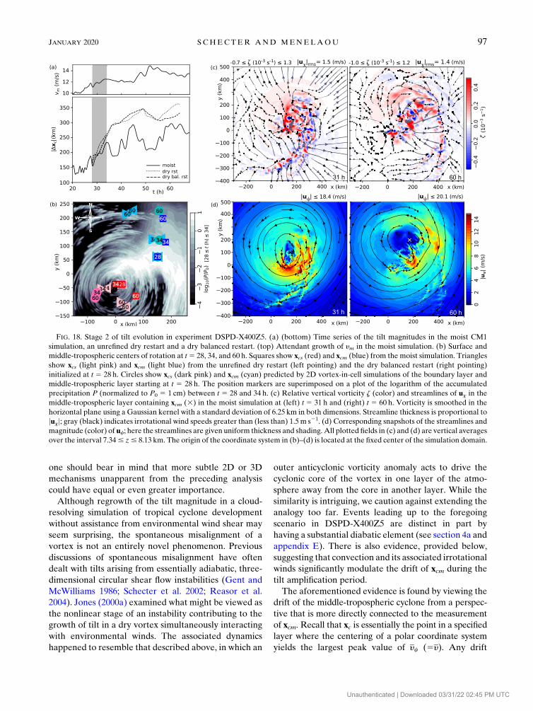
b. Stage 2

The subsequent regrowth of tilt in experiment

DSPD-X400Z5 occurs gradually over a 2-day period of

modest intensification of ym. The first issue we address

is whether moisture has an essential role in the process.

Figure 18a compares the growth of jDxcj to that found

in two dry adiabatic restarts at t 5 28 h. Two methods

are used for restarting the model to demonstrate that

details have little consequence on the result. The

first restart eliminates cloud microphysics, dissipative

heating and the surface enthalpy flux without any ad-

ditional modifications. The second restart also reduces

Cd to 2.5 3 1025 and refines the fluid variables. The

velocity field is refined by zeroing w, the irrotational

component of u, and the z-dependent horizontal mean

of u. The nondivergent component of u is obtained by

inverting z, adjusted to have zero vertical gradient in a

303-m layer adjacent to the sea surface. The final

refinement involves enforcing conditions of nonlinear

balance on u and the pressure field (see appendix C).

Both restarts demonstrate that the system would have a

propensity to increase tilt under dry adiabatic dynamics

somewhat faster and more effectively than the actual

process occurs amid moist convection.

Figure 18b compares the moist and dry trajectories of

xcs and xcm. The middle-tropospheric vortex centers of

the dry CM1 simulations move northward with their

moist counterpart, but drift farther to the west. Early on,

the surface center of the moist system is strongly in-

hibited from following any dry inclination to move

southwest. Such inhibition is consistent with the com-

mon attraction of surface centers toward areas of vigor-

ous deep convection, here situated to the northeast of xcs.

Figure 18b also shows the trajectories predicted by

ideal 2D fluid dynamics. The 2D results come from

two separate vortex-in-cell simulations (Leonard

1980) initialized with z distributions obtained from

the pertinent surface and middle-tropospheric layers

of the atmosphere at t 5 28 h. Each vortex-in-cell

simulation has roughly 108 vorticity elements, a rect-

angular mesh with 0.65-km grid spacing, and doubly

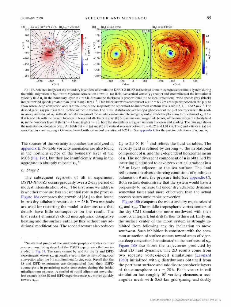
FIG. 16. Selected images of the boundary layer flow of simulationDSPD-X400Z5 in the fixed domain-centered coordinate systemduring

the initial migration of xcs toward vigorous convection downtilt. (a) Relative vertical vorticity z (color) and streamlines of the irrotational

velocity field ux in the boundary layer at t 5 6 h. Streamline thickness is proportional to the local irrotational wind speed; gray (black)

indicates wind speeds greater than (less than) 2.0m s21. Thin black arrowless contours of w at z5 8.9 km are superimposed on the plot to

show where deep convection occurs at the time of the snapshot; the outermost-to-innermost contour levels are 0.2, 1, 3, and 5m s21. The

dashed green ray points in the direction of the tilt vector. The ‘‘rms’’ statistic above the top-right corner of the plot corresponds to the root-

mean-square value of juxj in the depicted subregion of the simulation domain. The integers printed inside the plot show the location of xcs at t50, 4, 6, and 8 h, with the present location in black and all others in gray. (b) Streamlines andmagnitude (color) of the nondivergent velocity field

uc in the boundary layer at (left) t5 4 h and (right) t5 8 h; here the streamlines are given uniform thickness and shading. The plus sign shows

the instantaneous location of xcs. All fields butw in (a) and (b) are vertical averages between z5 0.025 and 1.01 km. The z andw fields in (a) are

smoothed in x and y using a Gaussian kernel with a standard deviation of 6.25 km. See appendix C for the precise definitions of ux and uc.

6 Substantial jumps of the middle-tropospheric vortex centers

are common during stage 1 of the DSPD experiments that are in-

cluded in Fig. 14. The same cannot be said for the IS and ISPD

experiments, where xcm generally starts in the vicinity of vigorous

convection after the 6-h misalignment forcing ends. Recall that the

IS and ISPD experiments are distinguished from their DSPD

counterparts in permitting moist convection during the initial

misalignment process. A period of rapid alignment neverthe-

less ensues in the IS and ISPD experiments as xcs moves quickly

toward xcm.



periodic boundary conditions equivalent to thoseof theCM1

simulations.Themiddle-tropospheric trajectorypredictedby

2D dynamics remains relatively close to that of the moist

system. Such closeness may be somewhat coincidental, but

reproduction of the basic northward drift suggests some

relevance of the 2D model. By contrast, the 2D surface

trajectory strays considerably from itsmoist counterpart, and

ends up far west of all 3D systems.

Figures 18c and 18d show snapshots of the moist

middle-tropospheric vortex near the start and end of the

northward drift of xcm that is largely responsible for the

regrowth of tilt. It is seen that the drift coincides with

considerable reshaping of an asymmetric vertical vorticity

distribution with multiscale structure and a prominent

band extending outward from the core. The process occurs

amid continual 3D-adiabatic and diabatic perturbations of

z. The associated irrotational winds represented by ux are

nontrivial (Fig. 18c), but as for any predominantly vortical

flow, the nondivergent component of the velocity field ucis characteristically stronger (Fig. 18d). The root-mean-

square (rms) value of jucj is 3.4 times the rms value of juxjover the depicted area in both snapshots.7

The relative strength of uc combined with the qualita-

tively successful prediction of the vortex-in-cell simulation

in the middle troposphere motivate further consideration

of how nondivergent 2D dynamics may contribute to the

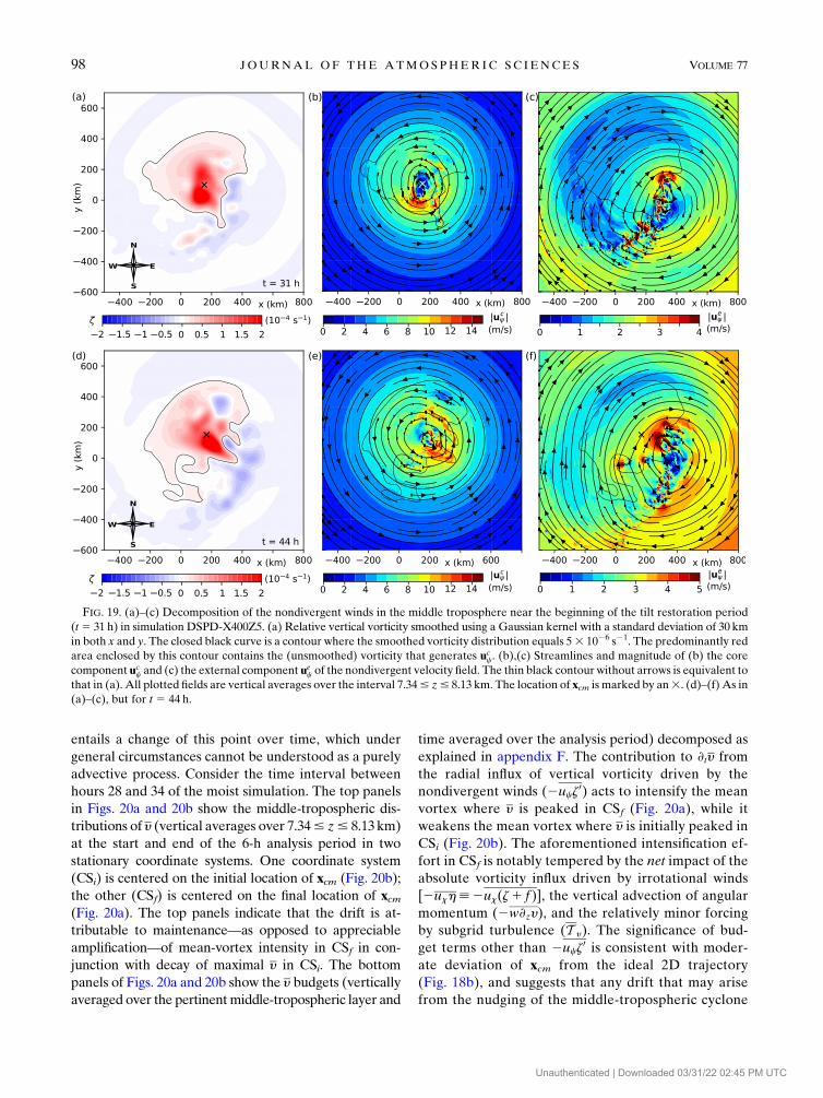
drift of xcm. Figure 19 splits the middle-tropospheric

nondivergent velocity field into two parts during the

northward drift period. The first part ucc is obtained by

inverting the unfiltered vertical vorticity distribution

inside the closed black curve in Fig. 19a (at t 5 31h) or

Fig. 19d (at t 5 44h) using a free-space Green function.

The aforementioned curve is essentially a contour where

z5 53 1026 s21 after Gaussian smoothing with a kernel

whose decay length is 30 km in both horizontal di-

mensions. By design, ucc (Figs. 19b,e) represents the

nondivergent winds of the predominantly cyclonic core

of the middle-tropospheric vortex. The second part is

defined by uec [ uc 2 uc

c (Figs. 19c,f) and represents the

nondivergent winds of structures external to the core.8

It is seen that negative vorticity to the east generates an

anticyclonic gyre in uec that alone would nudge the bulk

of the cyclonic core toward the north (northeast).9 Such

nudging does not seem incidental to the drift of xcm, but

FIG. 17. Selected images associatedwith the abrupt reduction of tilt during stage 1 of simulationDSPD-X400Z5. (a) Surface andmiddle-

tropospheric centers of rotation [xcs (red1) and xcm (blue3)] plotted every 30min over the interval 8.0# t# 9.5 h. The centermarkers are

superimposed on a plot of the logarithm of the accumulated precipitation P (normalized to P0 5 1 cm) during the aforementioned 1.5-h

time interval. Yellow symbols highlight xcm immediately before (circle) and after (diamond) it jumps to an area of enhanced precipitation.

(b),(c) Vertical averages of the relative vertical vorticity distribution z immediately after the rapid reduction of tilt (t5 9.5 h) in (b) the 1-

km surface boundary layer and (c) themiddle-tropospheric layer between z5 7.34 and 8.13 km.A contour plot of the vertical velocity field

w at z5 8.9 km (averaged over 8# t# 9.5 h) is superimposed on each vorticity distribution. Both z and w are smoothed in the horizontal

plane using a Gaussian kernel with a standard deviation of 6.25 km in both dimensions. The1 and3 in (b) and (c) respectively mark xcsand xcm at the time of the vorticity snapshot. The origin of the coordinate system in each plot corresponds to the fixed center of the

simulation domain.

7 The domain-averaged velocity ua—the third component of the

Helmholtz decomposition (appendixC) viewed in theES reference

frame—has a negligible magnitude of 0.1m s21 in the layer con-

taining xcm.

8 As such, uec includes minor contributions from images of the

core associated with periodic boundary conditions.9We have verified that similar scenarios unfold in the middle

troposphere during the regrowth of the misalignments in IS-

X400Z5 and ISPD-X400Z5, which have comparable initial tilt

magnitudes. Thus, the eastern anticyclonic vorticity patch does not

appear to be a unique consequence of the DSPD method for

generating the initial misalignment.



one should bear in mind that more subtle 2D or 3D

mechanisms unapparent from the preceding analysis

could have equal or even greater importance.

Although regrowth of the tilt magnitude in a cloud-

resolving simulation of tropical cyclone development

without assistance from environmental wind shear may

seem surprising, the spontaneous misalignment of a

vortex is not an entirely novel phenomenon. Previous

discussions of spontaneous misalignment have often

dealt with tilts arising from essentially adiabatic, three-

dimensional circular shear flow instabilities (Gent and

McWilliams 1986; Schecter et al. 2002; Reasor et al.

2004). Jones (2000a) examined what might be viewed as

the nonlinear stage of an instability contributing to the

growth of tilt in a dry vortex simultaneously interacting

with environmental winds. The associated dynamics

happened to resemble that described above, in which an

outer anticyclonic vorticity anomaly acts to drive the

cyclonic core of the vortex in one layer of the atmo-

sphere away from the core in another layer. While the

similarity is intriguing, we caution against extending the

analogy too far. Events leading up to the foregoing

scenario in DSPD-X400Z5 are distinct in part by

having a substantial diabatic element (see section 4a and

appendix E). There is also evidence, provided below,

suggesting that convection and its associated irrotational

winds significantly modulate the drift of xcm during the

tilt amplification period.

The aforementioned evidence is found by viewing the

drift of the middle-tropospheric cyclone from a perspec-

tive that is more directly connected to the measurement

of xcm. Recall that xc is essentially the point in a specified

layer where the centering of a polar coordinate system

yields the largest peak value of yc (5y). Any drift

FIG. 18. Stage 2 of tilt evolution in experiment DSPD-X400Z5. (a) (bottom) Time series of the tilt magnitudes in the moist CM1

simulation, an unrefined dry restart and a dry balanced restart. (top) Attendant growth of ym in the moist simulation. (b) Surface and

middle-tropospheric centers of rotation at t5 28, 34, and 60 h. Squares show xcs (red) and xcm (blue) from the moist simulation. Triangles

show xcs (light pink) and xcm (light blue) from the unrefined dry restart (left pointing) and the dry balanced restart (right pointing)

initialized at t 5 28 h. Circles show xcs (dark pink) and xcm (cyan) predicted by 2D vortex-in-cell simulations of the boundary layer and

middle-tropospheric layer starting at t 5 28 h. The position markers are superimposed on a plot of the logarithm of the accumulated

precipitation P (normalized to P0 5 1 cm) between t 5 28 and 34 h. (c) Relative vertical vorticity z (color) and streamlines of ux in the

middle-tropospheric layer containing xcm (3) in the moist simulation at (left) t 5 31 h and (right) t 5 60 h. Vorticity is smoothed in the

horizontal plane using a Gaussian kernel with a standard deviation of 6.25 km in both dimensions. Streamline thickness is proportional to

juxj; gray (black) indicates irrotational wind speeds greater than (less than) 1.5m s21. (d) Corresponding snapshots of the streamlines and

magnitude (color) of uc; here the streamlines are given uniform thickness and shading.All plotted fields in (c) and (d) are vertical averages

over the interval 7.34# z# 8.13 km. The origin of the coordinate system in (b)–(d) is located at the fixed center of the simulation domain.



entails a change of this point over time, which under

general circumstances cannot be understood as a purely

advective process. Consider the time interval between

hours 28 and 34 of the moist simulation. The top panels

in Figs. 20a and 20b show the middle-tropospheric dis-

tributions of y (vertical averages over 7.34# z# 8.13km)

at the start and end of the 6-h analysis period in two

stationary coordinate systems. One coordinate system

(CSi) is centered on the initial location of xcm (Fig. 20b);

the other (CSf) is centered on the final location of xcm(Fig. 20a). The top panels indicate that the drift is at-

tributable to maintenance—as opposed to appreciable

amplification—of mean-vortex intensity in CSf in con-

junction with decay of maximal y in CSi. The bottom

panels of Figs. 20a and 20b show the y budgets (vertically

averaged over the pertinentmiddle-tropospheric layer and

time averaged over the analysis period) decomposed as

explained in appendix F. The contribution to ›ty from

the radial influx of vertical vorticity driven by the

nondivergent winds (2ucz0) acts to intensify the mean

vortex where y is peaked in CSf (Fig. 20a), while it

weakens the mean vortex where y is initially peaked in

CSi (Fig. 20b). The aforementioned intensification ef-

fort in CSf is notably tempered by the net impact of the

absolute vorticity influx driven by irrotational winds

[2uxh[2ux(z1 f )], the vertical advection of angular

momentum (2w›zy), and the relatively minor forcing

by subgrid turbulence (T y). The significance of bud-

get terms other than 2ucz0 is consistent with moder-

ate deviation of xcm from the ideal 2D trajectory

(Fig. 18b), and suggests that any drift that may arise

from the nudging of the middle-tropospheric cyclone

FIG. 19. (a)–(c) Decomposition of the nondivergent winds in the middle troposphere near the beginning of the tilt restoration period

(t5 31 h) in simulation DSPD-X400Z5. (a) Relative vertical vorticity smoothed using a Gaussian kernel with a standard deviation of 30 km

in both x and y. The closed black curve is a contour where the smoothed vorticity distribution equals 53 1026 s21. The predominantly red

area enclosed by this contour contains the (unsmoothed) vorticity that generates ucc. (b),(c) Streamlines and magnitude of (b) the core

component ucc and (c) the external component ue

c of the nondivergent velocity field. The thin black contour without arrows is equivalent to

that in (a). All plotted fields are vertical averages over the interval 7.34# z# 8.13 km. The location of xcm is marked by an3. (d)–(f) As in

(a)–(c), but for t 5 44 h.



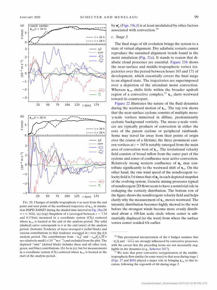
by uec (Figs. 19c,f) is at least modulated by other factors

associated with convection.10

c. Stage 3

The final stage of tilt evolution brings the system to a

state of virtual alignment. Dry adiabatic restarts cannot

reproduce the sustained alignment trends found in the

moist simulation (Fig. 21a). It stands to reason that di-

abatic cloud processes are essential. Figure 21b shows

the near-surface and middle-tropospheric vortex tra-

jectories over the period between hours 165 and 171 of

development, which essentially covers the final surge

to an aligned state. The trajectories are superimposed

over a depiction of the attendant moist convection.

Whereas xcm shifts little within the broader updraft

region of a convective complex,11 xcs darts westward

toward its counterpart.

Figure 22 illustrates the nature of the fluid dynamics

during the westward motion of xcs. The top row shows

that the near-surface cyclone consists of multiple meso-

g-scale vortices immersed in diffuse, predominantly

cyclonic background vorticity. The meso-g-scale vorti-

ces are typically products of convection in either the

core of the parent cyclone or peripheral rainbands.

Some may travel far away from their points of origin

over the course of a lifetime; the three prominent east-

ern vortices at t5 165h notably emerged from the main

area of convection west of xcs. The irrotational velocity

field consists of broad inflow from the outer part of the

cyclone and zones of confluence near active convection.

Relatively strong western confluence of ux may con-

tribute significantly to the westward shift of xcs. On the

other hand, the rms wind speed of the nondivergent ve-

locity field is 5.6 times that ofux in each depicted snapshot

of the evolving system. Generic mixing processes typical

of nondivergent 2Dflows seem to have a nontrivial role in

reshaping the vorticity distribution. The bottom row of

the figure shows the nondivergent velocity field and helps

clarify why the measurement of xcs moves westward. The

intensity distribution becomes highly skewed to the west

before the strongest winds become more evenly distrib-

uted about a 100-km scale circle whose center is sub-

stantially displaced (to the west) from where the surface

vortex center resided 6h earlier.

FIG. 20. Changes of middle-tropospheric y as seen from the end

point and start point of the northward trajectory of xcm in simula-

tion DSPD-X400Z5 during the shaded time interval in Fig. 18a (28

# t # 34 h). (a) (top) Snapshots of y (averaged between z 5 7.34

and 8.13 km) measured in a coordinate system (CSf) centered

where xcm is located at the end of the analysis period. The solid

(dashed) curve corresponds to y at the end (start) of the analysis

period. (bottom) Tendency of layer-averaged y (solid black) and

various contributions to that tendency averaged in t over the 6-h

analysis period. The contributions from 2uaz0 and 2cpdu

0r›uP

0/r

are relatively small (�1024 m s22) and excluded from the plot. The

depicted ‘‘sum’’ (dotted black) includes these and all other (red,

green, and blue) contributions. (b) As in (a), but for measurements

in a coordinate system (CSi) centered where xcm is located at the

start of the analysis period.

10 This provisional interpretation of the y budget assumes that

2uxh and 2w›zy are strongly influenced by convective processes,

with the caveat that the preceding terms are not necessarily neg-

ligible in dry dynamics (e.g., Schecter 2017).11We note that prior convective reorganization of the middle-

tropospheric flow similar (in some ways) to that seen during stage 1

(Figs. 17 and B1b) played a major role in bringing xcm to this lo-

cation, following the regrowth of tilt during stage 2.



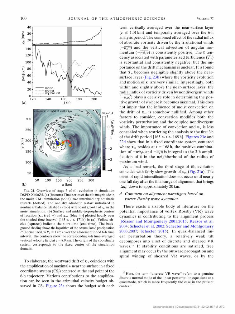
To elaborate, the westward drift of xcs coincides with

the amplification of maximal y near the surface in a fixed

coordinate system (CSf) centered at the end point of the

6-h trajectory. Various contributions to the amplifica-

tion can be seen in the azimuthal velocity budget ob-

served in CSf. Figure 23a shows the budget with each

term vertically averaged over the near-surface layer

(z # 1.01 km) and temporally averaged over the 6-h

analysis period. The combined effect of the radial influx

of absolute vorticity driven by the irrotational winds

(2uxh) and the vertical advection of angular mo-

mentum (2w›zy) is consistently positive. The y ten-

dency associated with parameterized turbulence (T y)

is substantial and consistently negative, but the im-

portance on the drift mechanism is unclear. It is found

that T y becomes negligible slightly above the near-

surface layer (Fig. 23b) where the vorticity evolution

and motion of xc are very similar. Interestingly, both

within and slightly above the near-surface layer, the

radial influx of vorticity driven by nondivergent winds

(2ucz0) plays a decisive role in determining the pos-

itive growth of y where it becomes maximal. This does

not imply that the influence of moist convection on

the drift of xcs is somehow nullified. Among other

factors to consider, convection modifies both the

vorticity perturbation and the coupled nondivergent

winds. The importance of convection and ux is less

concealed when restricting the analysis to the first 3 h

of the drift period [165 # t # 168 h]. Figures 23c and

22d show that in a fixed coordinate system centered

where xcs resides at t 5 168 h, the positive combina-

tion of 2w›zy and 2uxh is integral to the 3-h ampli-

fication of y in the neighborhood of the radius of

maximum wind.

As a final remark, the third stage of tilt evolution

coincides with fairly slow growth of ym (Fig. 21a). The

onset of rapid intensification does not occur until nearly

one full day after the final surge of alignment that brings

jDxcj down to approximately 20 km.

d. Comment on alignment paradigms based onvortex Rossby wave dynamics

There exists a sizable body of literature on the

potential importance of vortex Rossby (VR) wave

dynamics in contributing to the alignment process

(Reasor and Montgomery 2001,2015; Reasor et al.

2004; Schecter et al. 2002; Schecter and Montgomery

2003,2007; Schecter 2015). In quasi-balanced lin-

ear perturbation theory, a relatively weak tilt

decomposes into a set of discrete and sheared VR

waves.12 If stability conditions are satisfied, free

alignment may occur by the outward propagation and

spiral windup of sheared VR waves, or by the

FIG. 21. Overview of stage 3 of tilt evolution in simulation

DSPD-X400Z5. (a) (bottom) Time series of the tilt magnitude in

the moist CM1 simulation (solid), two unrefined dry adiabatic

restarts (dotted), and one dry adiabatic restart initialized in

nonlinear balance (dashed). (top) Attendant growth of ym in the

moist simulation. (b) Surface and middle-tropospheric centers

of rotation [xcs (red 1) and xcm (blue 3)] plotted hourly over

the shaded time interval (165 # t # 171 h) in (a). Yellow cir-

cles (squares) indicate the start time (end time). The back-

ground shading shows the logarithm of the accumulated precipitation

P (normalized to P0 5 1 cm) over the aforementioned 6-h time

interval. The contours show the corresponding 6-h time-averaged

vertical velocity field at z5 8.9 km. The origin of the coordinate

system corresponds to the fixed center of the simulation

domain.

12 Here, the term ‘‘discrete VR wave’’ refers to a genuine

discrete normal mode of the linear perturbation equations or a

quasimode, which is more frequently the case in the present

context.



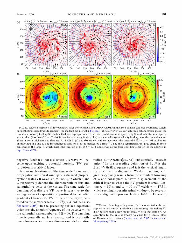
negative feedback that a discrete VR wave will re-

ceive upon exciting a potential vorticity (PV) per-

turbation in a critical layer.

A reasonable estimate of the time scale for outward

propagation and spiral windup of a sheared (tropical

cyclone scale) VR wave is ty[ 2pry/yy, in which ry and

yy respectively denote the characteristic radius and

azimuthal velocity of the vortex. The time scale for

damping of a discrete VR wave is sensitive to the

average value of a quantity proportional to the radial

gradient of basic-state PV in the critical layer, cen-

tered on the surface where v5 nV(r, z) (ibid., see also

Schecter 2008). In the preceding surface equation,

v denotes the angular frequency of the wave, n 5 1 is

the azimuthal wavenumber, andV[ y/r. The damping

time is generally no less than ty, and is ordinarily

much longer when the nondimensional deformation

radius ‘d [NH/max[2yy , ryf ] substantially exceeds

unity.13 In the preceding definition of ‘d, N is the

Brunt–Väisälä frequency and H is the vertical length

scale of the misalignment. Weaker damping with

greater ‘d partly results from the attendant lowering

of v and consequent outward displacement of the

critical layer to where the PV gradient is small. Let-

ting ry 5 105m and yy 5 10m s21 yields ty 5 17.5 h,

which seemingly permits spiral windup to be relevant

to an alignment process lasting 1–10 d. However,

FIG. 22. Selected snapshots of the boundary layer flow of simulation DSPD-X400Z5 in the fixed domain-centered coordinate system

during the final surge toward alignment (the shaded time interval in Fig. 21a). (a) Relative vertical vorticity z (color) and streamlines of the

irrotational velocity field ux. Streamline thickness is proportional to the local irrotational wind speed; gray (black) indicates wind speeds

greater than (less than) 2.5m s21. (b) Streamlines and magnitude (color) of the nondivergent velocity field uc; here the streamlines are

given uniform thickness and shading. All fields in (a) and (b) are vertical averages over the interval 0.025 # z # 1.01 km but are

unsmoothed in x and y. The instantaneous location of xcs is marked by a small 1. The thick semitransparent gray circle in (b) is

centered on the large 1, which marks the location of xcs at t 5 171 h and serves as the fixed coordinate center for the analysis in

Figs. 23a and 23b.

13Weaker damping with greater ‘d is a rule-of-thumb that

applies to vortices with relatively smooth (e.g., Gaussian) PV

distributions that decay monotonically with increasing r. An

exception to the rule is known to exist for a special class

of Rankine-like vortices (Schecter et al. 2002; Schecter and

Montgomery 2003).



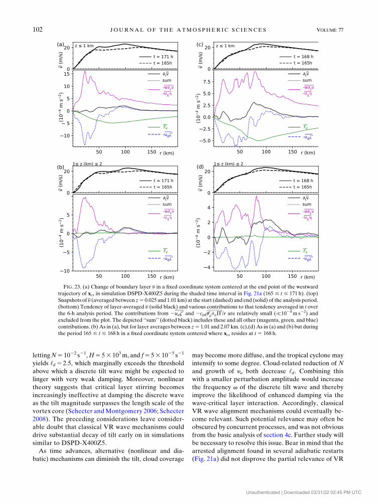
lettingN5 1022 s21,H5 53 103m, and f5 53 1025 s21

yields ‘d 5 2:5, which marginally exceeds the threshold

above which a discrete tilt wave might be expected to

linger with very weak damping. Moreover, nonlinear

theory suggests that critical layer stirring becomes

increasingly ineffective at damping the discrete wave

as the tilt magnitude surpasses the length scale of the

vortex core (Schecter andMontgomery 2006; Schecter

2008). The preceding considerations leave consider-

able doubt that classical VR wave mechanisms could

drive substantial decay of tilt early on in simulations

similar to DSPD-X400Z5.

As time advances, alternative (nonlinear and dia-

batic) mechanisms can diminish the tilt, cloud coverage

may become more diffuse, and the tropical cyclone may

intensify to some degree. Cloud-related reduction of N

and growth of yy both decrease ‘d. Combining this

with a smaller perturbation amplitude would increase

the frequency v of the discrete tilt wave and thereby

improve the likelihood of enhanced damping via the

wave-critical layer interaction. Accordingly, classical

VR wave alignment mechanisms could eventually be-

come relevant. Such potential relevance may often be

obscured by concurrent processes, and was not obvious

from the basic analysis of section 4c. Further study will

be necessary to resolve this issue. Bear in mind that the

arrested alignment found in several adiabatic restarts

(Fig. 21a) did not disprove the partial relevance of VR

FIG. 23. (a) Change of boundary layer y in a fixed coordinate system centered at the end point of the westward

trajectory of xcs in simulation DSPD-X400Z5 during the shaded time interval in Fig. 21a (165 # t # 171 h). (top)

Snapshots of y (averaged between z5 0.025 and 1.01 km) at the start (dashed) and end (solid) of the analysis period.

(bottom) Tendency of layer-averaged y (solid black) and various contributions to that tendency averaged in t over

the 6-h analysis period. The contributions from 2uaz0 and 2cpdu

0r›uP

0/r are relatively small (�1024 m s22) and

excluded from the plot. The depicted ‘‘sum’’ (dotted black) includes these and all other (magenta, green, and blue)

contributions. (b) As in (a), but for layer averages between z5 1.01 and 2.07 km. (c),(d)As in (a) and (b) but during

the period 165 # t # 168 h in a fixed coordinate system centered where xcs resides at t 5 168 h.



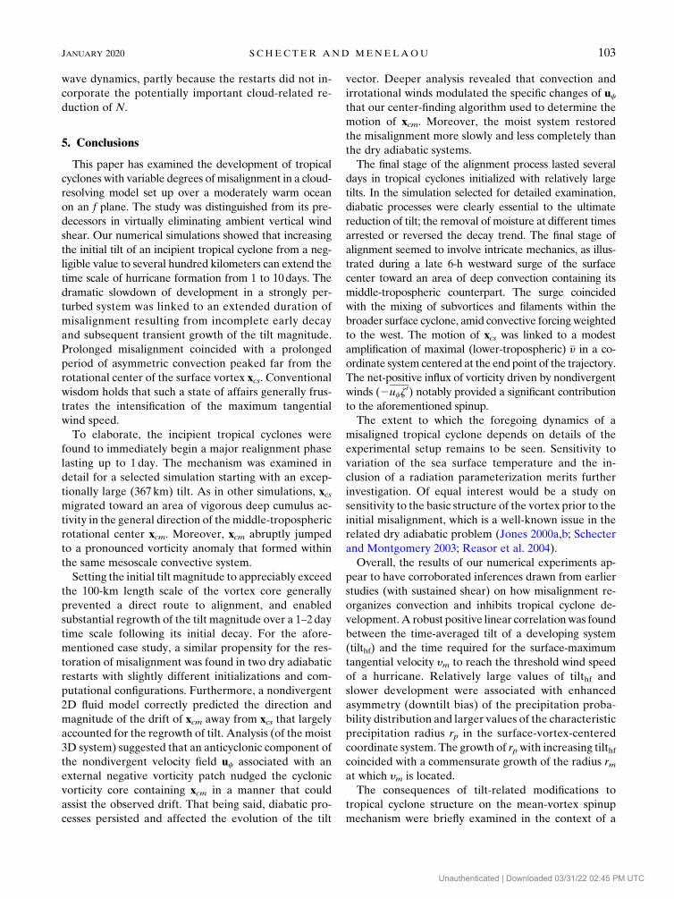
wave dynamics, partly because the restarts did not in-

corporate the potentially important cloud-related re-

duction of N.

5. Conclusions

This paper has examined the development of tropical

cyclones with variable degrees of misalignment in a cloud-

resolving model set up over a moderately warm ocean

on an f plane. The study was distinguished from its pre-

decessors in virtually eliminating ambient vertical wind

shear. Our numerical simulations showed that increasing

the initial tilt of an incipient tropical cyclone from a neg-

ligible value to several hundred kilometers can extend the

time scale of hurricane formation from 1 to 10days. The

dramatic slowdown of development in a strongly per-

turbed system was linked to an extended duration of

misalignment resulting from incomplete early decay

and subsequent transient growth of the tilt magnitude.

Prolonged misalignment coincided with a prolonged

period of asymmetric convection peaked far from the

rotational center of the surface vortex xcs. Conventional

wisdom holds that such a state of affairs generally frus-

trates the intensification of the maximum tangential

wind speed.

To elaborate, the incipient tropical cyclones were

found to immediately begin a major realignment phase

lasting up to 1day. The mechanism was examined in

detail for a selected simulation starting with an excep-

tionally large (367 km) tilt. As in other simulations, xcsmigrated toward an area of vigorous deep cumulus ac-

tivity in the general direction of themiddle-tropospheric

rotational center xcm. Moreover, xcm abruptly jumped

to a pronounced vorticity anomaly that formed within

the same mesoscale convective system.

Setting the initial tilt magnitude to appreciably exceed

the 100-km length scale of the vortex core generally

prevented a direct route to alignment, and enabled

substantial regrowth of the tilt magnitude over a 1–2day

time scale following its initial decay. For the afore-

mentioned case study, a similar propensity for the res-

toration of misalignment was found in two dry adiabatic

restarts with slightly different initializations and com-

putational configurations. Furthermore, a nondivergent

2D fluid model correctly predicted the direction and

magnitude of the drift of xcm away from xcs that largely

accounted for the regrowth of tilt. Analysis (of the moist

3D system) suggested that an anticyclonic component of

the nondivergent velocity field uc associated with an

external negative vorticity patch nudged the cyclonic

vorticity core containing xcm in a manner that could

assist the observed drift. That being said, diabatic pro-

cesses persisted and affected the evolution of the tilt

vector. Deeper analysis revealed that convection and

irrotational winds modulated the specific changes of ucthat our center-finding algorithm used to determine the

motion of xcm. Moreover, the moist system restored

the misalignment more slowly and less completely than

the dry adiabatic systems.

The final stage of the alignment process lasted several

days in tropical cyclones initialized with relatively large

tilts. In the simulation selected for detailed examination,

diabatic processes were clearly essential to the ultimate

reduction of tilt; the removal of moisture at different times

arrested or reversed the decay trend. The final stage of

alignment seemed to involve intricate mechanics, as illus-

trated during a late 6-h westward surge of the surface

center toward an area of deep convection containing its

middle-tropospheric counterpart. The surge coincided

with the mixing of subvortices and filaments within the

broader surface cyclone, amid convective forcing weighted

to the west. The motion of xcs was linked to a modest

amplification of maximal (lower-tropospheric) y in a co-

ordinate system centered at the end point of the trajectory.

The net-positive influx of vorticity driven by nondivergent

winds (2ucz0) notably provided a significant contribution

to the aforementioned spinup.

The extent to which the foregoing dynamics of a

misaligned tropical cyclone depends on details of the

experimental setup remains to be seen. Sensitivity to

variation of the sea surface temperature and the in-

clusion of a radiation parameterization merits further

investigation. Of equal interest would be a study on

sensitivity to the basic structure of the vortex prior to the

initial misalignment, which is a well-known issue in the

related dry adiabatic problem (Jones 2000a,b; Schecter

and Montgomery 2003; Reasor et al. 2004).

Overall, the results of our numerical experiments ap-

pear to have corroborated inferences drawn from earlier

studies (with sustained shear) on how misalignment re-

organizes convection and inhibits tropical cyclone de-

velopment.A robust positive linear correlationwas found

between the time-averaged tilt of a developing system

(tilthf) and the time required for the surface-maximum

tangential velocity ym to reach the threshold wind speed

of a hurricane. Relatively large values of tilthf and

slower development were associated with enhanced

asymmetry (downtilt bias) of the precipitation proba-

bility distribution and larger values of the characteristic

precipitation radius rp in the surface-vortex-centered

coordinate system. The growth of rpwith increasing tilthfcoincided with a commensurate growth of the radius rmat which ym is located.

The consequences of tilt-related modifications to

tropical cyclone structure on the mean-vortex spinup

mechanism were briefly examined in the context of a



Sawyer–Eliassen (SE) model. The SE-based analysis

provided a reasonably accurate decomposition of the

early azimuthal velocity tendency in the vicinity of ym, in

selected systems with low and high degrees of mis-

alignment. Although no single factor completely ex-

plained slower intensification in the strongly misaligned

system, greater tilt was linked to weaker positive azi-

muthal velocity forcing near ym by the component of the

mean secondary circulation attributed to heating by

microphysical cloud processes.

One notable aspect of the present simulation set

was minimal system-to-system variation in the growth

of kinetic energy contained outside the core of the

primary surface circulation over the time scale re-

quired for an aligned vortex to mature. In other

words, the detrimental effect of tilt on surface kinetic

energy growth was confined to the inner region of the

surface vortex.

We conclude with a final remark on the relevance of

this paper to forecasting. Although a strong correla-

tion was found between tilthf and thf, our results sug-

gest that an instantaneous measurement of the tilt

magnitude may not be a good predictor of the time

scale for future intensification of ym, even in a quies-

cent environment. Such is evident from the non-

monotonic evolution of the tilt magnitude. Distinct

time scales would be found for equivalent magnitudes

measured during different growth or decay phases of

the misalignment.

Acknowledgments. The authors thank Dr. George

Bryan of the National Center for Atmospheric Re-

search (NCAR) for providing the cloud-resolving

model (CM1) that was used for the numerical experi-

ments. The authors also thank several anonymous re-

viewers for their generally constructive comments on

the submitted manuscript. This paper was primarily

supported by the National Science Foundation under

Grant AGS-1743854. Additional support came from

the Natural Sciences and Engineering Research

Council of Canada, and from Hydro-Quebec through

the IRC program. The computational resources re-

quired to conduct the simulations were provided by

NCAR’s Computational and Information Systems Labo-

ratory (doi:10.5065/D6RX99HX), and by Compute Canada.

APPENDIX A

Vortex States Generated by ArtificialMisalignment Forcing

Figure A1 depicts a number of selected vortices im-

mediately after their misalignments are generated by

methods explained in section 2a. Figures A1a and A1b

show a vortex that is misaligned using the DSPD

method, with zl 5 5.25 km and a target tilt magnitude

of 400 km. The top panel shows relative vertical vorticity

and relative humidity in a vertical plane parallel to the

tilt vector [Eq. (4)] and passing through the surface

vortex center. Both fields are 500-km centered averages

over the coordinate y0 that measures horizontal distance

perpendicular to the visualization plane. The relative

humidity assumes ice (liquid) condensate above (below)

the freezing level. The bottom panel shows horizontal

slices of lower- and middle-tropospheric vorticity.

Note that the misalignment process 1) reduces middle-

tropospheric relative humidity over the central and uptilt

regions of the surface vortex, and 2) reweights the nega-

tive component of the vorticity distribution toward the

east in the outer part of themiddle-tropospheric circulation.

Figures A1c andA1d are similar to Figs. A1a andA1b, but

for a DSPD experiment with a target tilt magnitude of

100 km. Here, the aforementioned consequences of the

misalignment process are considerably less pronounced.

Figures A1e and A1f show the vortex from ISPD-

X400Z5, in which the tilt is generated while convection

is active over the first 6 h of the simulation. The mis-

alignment is moderately smaller than its counterpart in

the DSPD experiment with equivalent settings for the

target tilt magnitude and zl (Figs. A1a,b). The convec-

tion has also generated a dipole-asymmetry within the

predominantly cyclonic core of the middle-tropospheric

vortex. The intensity of the negative vorticity hole

within the core is found to decay with decreasing values

of the target tilt magnitude (not shown). Of further

note, as in the aforementioned DSPD experiment, the

misaligned vortex has diminished negative vorticity

in the outer western region of the middle troposphere.

Figures A1g and A1h are similar to Figs. A1e and A1f,

but for ISPD-X300Z3.

APPENDIX B

Sensitivity to the Center-Finding Algorithm

The ‘‘vortex center’’ at a specified altitude is not uniquely

defined in tropical cyclone meteorology. One might

wonder how changing the definition would affect the de-

scription of the dynamics. This appendix aims to remove

some of the mystery for the present study without an ex-

haustive sensitivity test.

Limited testing has shown that reducing lc in the stan-

dard center-finding algorithmof section 2b ordinarily adds

noise to the time series of xc without changing the main

trend over any extended time period of interest. The

preceding result seems obvious and unworthy of lengthy



https://doi.org/10.5065/D6RX99HX

discussion. Instead, let us consider the following al-

ternative definition of a cyclonic vortex center in an

arbitrary layer:

~xc[

ðA

xzQ(z2 zc) dAð

A

zQ(z2 zc) dA

, (B1)

in which the area A of integration covers the entire

horizontal domain of the simulation, x is the horizontal

coordinate vector, z is the z-averaged relative vertical

vorticity distribution of the pertinent layer smoothed as

in section 2bwith lc5 23.75 km, andQ(z2 zc)5 1 (0) for

z . zc (z , zc). The cut-off vorticity is given by

zc[ �

zmax(z) , (B2)

in which 0 , �z , 1.

Figure B1a compares the tilt magnitude in DSPD-

X400Z5 computed with our standard method to that

obtained by replacing xcs/cm with ~xcs/cm in Eq. (4). The

modification of the time series is modest for �z 5 0.1 but

nontrivial for �z 5 0.02. The greatest discrepancies begin

when vorticity anomalies generated by convection in

the middle troposphere create a sufficiently strong

meso-b-scale rotational flow structure far away from the

prior consensus vortex center (t ’ 10, 75 h). At such

times, the middle-tropospheric flow cannot be said to

consist of a single vortex.

Figures B1b–d show snapshots of the streamlines and

magnitude of the middle-tropospheric nondivergent

velocity field after an early event when the single vortex

model of the middle-tropospheric flow becomes ques-

tionable. The standard location of xcm (found as in sec-

tion 2b) and the locations of ~xcm obtained with �z 5 0.1

and 0.02 are indicated on each snapshot; so too are the

surface centers. The first snapshot (Fig. B1b) reveals

substantial differences between the standard computa-

tion of xcm and its alternatives. At this time, two

noteworthy mesoscale vortices exist. One is the large

northeastern cyclone originating from the initial con-

ditions, and the other is a small convectively generated

FIG. A1. Vortex states immediately after misalignments are generated [t 5 0 h (6 h) for DSPD (ISPD) experiments]. (a) Relative

vertical vorticity (color) and relative humidity (contours; %) in a vertical plane parallel to the tilt vector and passing through the surface

vortex center in experiment DSPD-X400Z5. (b) Relative vertical vorticity at z 5 1.0 km (z1; color) and z 5 7.7 km (z7.7; contours). The

contour labels are in units of 1024 s21. The locations of the surface and middle-tropospheric vortex centers (xcs and xcm defined in section

2b) are marked by the symbols1 and 3, respectively. The green x0 (y0) axis runs parallel (perpendicular) to the tilt vector, which points

from 1 to 3. The fields in (a) are averaged over the 500-km distance between the depicted end-bars of the y0 axis; in addition, they are

smoothed using a Gaussian kernel with standard deviations of 6.25 km in x0 and 0.15 km in z. The fields in (b) are smoothed using a

Gaussian kernel with a standard deviation of 30 km in both x and y. (c),(d) As in (a) and (b), but for experiment DSPD-X100Z5. (e),(f) As

in (a) and (b), but for experiment ISPD-X400Z5. (g),(h) As in (a) and (b), but for experiment ISPD-X300Z3. The color bar to the right of

(g) applies to all panels in the top row. The contour levels in (d) are as in (b), whereas the contour levels in (h) are as in (f). The origin of the

coordinate system in each plot corresponds to the center of the surface vortex.



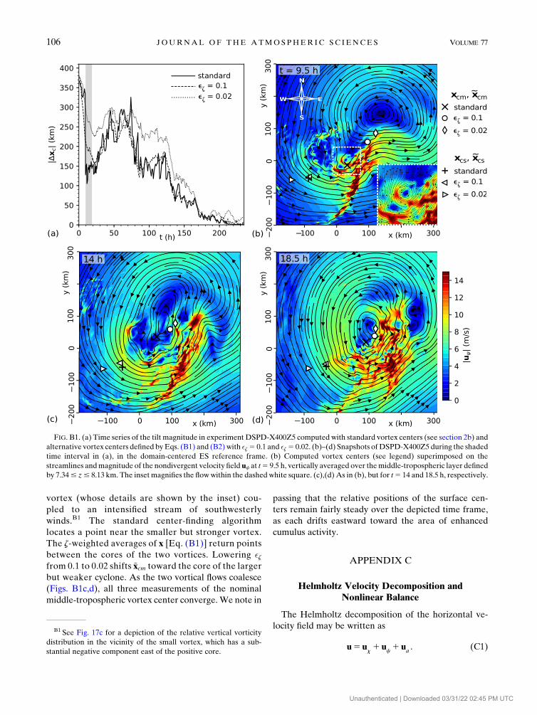
vortex (whose details are shown by the inset) cou-

pled to an intensified stream of southwesterly

winds.B1 The standard center-finding algorithm

locates a point near the smaller but stronger vortex.

The z-weighted averages of x [Eq. (B1)] return points

between the cores of the two vortices. Lowering �zfrom 0.1 to 0.02 shifts ~xcm toward the core of the larger

but weaker cyclone. As the two vortical flows coalesce

(Figs. B1c,d), all three measurements of the nominal

middle-tropospheric vortex center converge. We note in

passing that the relative positions of the surface cen-

ters remain fairly steady over the depicted time frame,

as each drifts eastward toward the area of enhanced

cumulus activity.

APPENDIX C

Helmholtz Velocity Decomposition andNonlinear Balance

The Helmholtz decomposition of the horizontal ve-

locity field may be written as

u5 ux1u

c1u

a. (C1)

FIG. B1. (a) Time series of the tilt magnitude in experiment DSPD-X400Z5 computed with standard vortex centers (see section 2b) and

alternative vortex centers defined byEqs. (B1) and (B2) with �z5 0.1 and �z5 0.02. (b)–(d) Snapshots ofDSPD-X400Z5 during the shaded

time interval in (a), in the domain-centered ES reference frame. (b) Computed vortex centers (see legend) superimposed on the

streamlines andmagnitude of the nondivergent velocity field uc at t5 9.5 h, vertically averaged over themiddle-tropospheric layer defined

by 7.34# z# 8.13 km. The inset magnifies the flowwithin the dashed white square. (c),(d) As in (b), but for t5 14 and 18.5 h, respectively.

B1 See Fig. 17c for a depiction of the relative vertical vorticity

distribution in the vicinity of the small vortex, which has a sub-

stantial negative component east of the positive core.



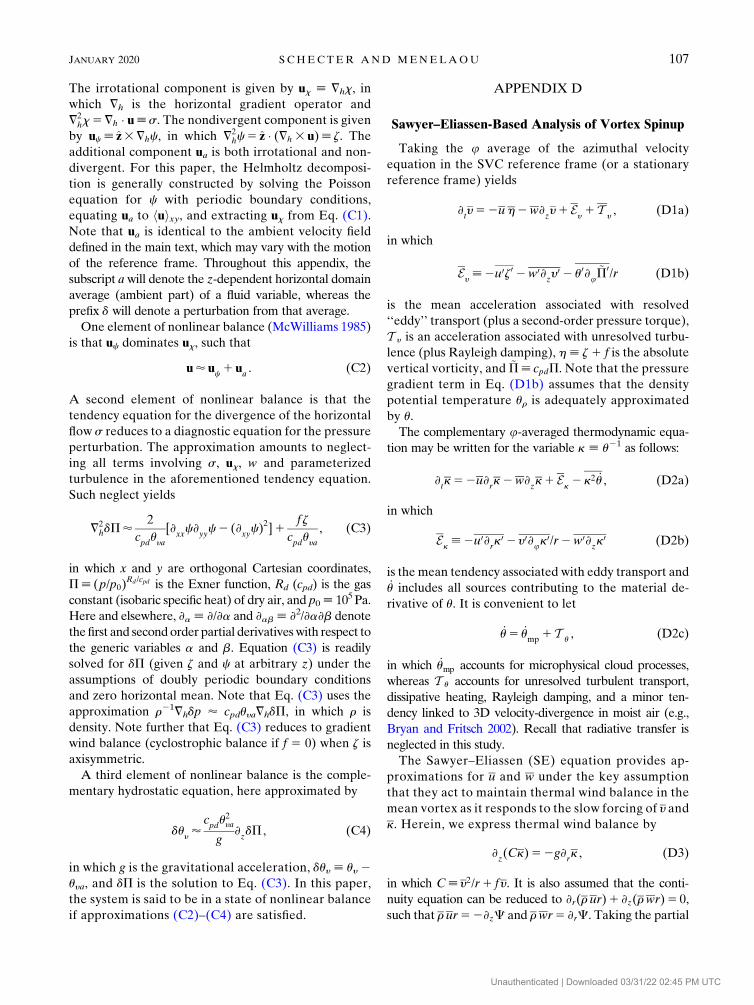
The irrotational component is given by ux [ =hx, in

which =h is the horizontal gradient operator and

=2hx5=h � u[s. The nondivergent component is given

by uc [ z3=hc, in which =2hc5 z � (=h 3 u)[ z. The

additional component ua is both irrotational and non-

divergent. For this paper, the Helmholtz decomposi-

tion is generally constructed by solving the Poisson

equation for c with periodic boundary conditions,

equating ua to huixy, and extracting ux from Eq. (C1).

Note that ua is identical to the ambient velocity field

defined in the main text, which may vary with the motion

of the reference frame. Throughout this appendix, the

subscript awill denote the z-dependent horizontal domain

average (ambient part) of a fluid variable, whereas the

prefix d will denote a perturbation from that average.

One element of nonlinear balance (McWilliams 1985)

is that uc dominates ux, such that

u’ uc1 u

a. (C2)

A second element of nonlinear balance is that the

tendency equation for the divergence of the horizontal

flow s reduces to a diagnostic equation for the pressure

perturbation. The approximation amounts to neglect-

ing all terms involving s, ux, w and parameterized

turbulence in the aforementioned tendency equation.

Such neglect yields

=2hdP’

2

cpduya

[›xxc›

yyc2 (›

xyc)2]1

f z

cpduya

, (C3)

in which x and y are orthogonal Cartesian coordinates,

P[ (p/p0)Rd/cpd is the Exner function, Rd (cpd) is the gas

constant (isobaric specific heat) of dry air, and p0[ 105Pa.

Here and elsewhere, ›a [ ›/›a and ›ab [ ›2/›a›b denote

the first and secondorder partial derivativeswith respect to

the generic variables a and b. Equation (C3) is readily

solved for dP (given z and c at arbitrary z) under the

assumptions of doubly periodic boundary conditions

and zero horizontal mean. Note that Eq. (C3) uses the

approximation r21=hdp ’ cpduya=hdP, in which r is

density. Note further that Eq. (C3) reduces to gradient

wind balance (cyclostrophic balance if f 5 0) when z is

axisymmetric.

A third element of nonlinear balance is the comple-

mentary hydrostatic equation, here approximated by

duy’

cpdu2ya

g›zdP , (C4)

in which g is the gravitational acceleration, duy [ uy 2uya, and dP is the solution to Eq. (C3). In this paper,

the system is said to be in a state of nonlinear balance

if approximations (C2)–(C4) are satisfied.

APPENDIX D

Sawyer–Eliassen-Based Analysis of Vortex Spinup

Taking the u average of the azimuthal velocity

equation in the SVC reference frame (or a stationary

reference frame) yields

›ty52uh2w›

zy1 E

y1 T

y, (D1a)

in which

Ey[2u0z0 2w0›

zy0 2 u0›u

~P0/r (D1b)

is the mean acceleration associated with resolved

‘‘eddy’’ transport (plus a second-order pressure torque),

T y is an acceleration associated with unresolved turbu-

lence (plus Rayleigh damping), h[ z1 f is the absolute

vertical vorticity, and ~P[ cpdP. Note that the pressure

gradient term in Eq. (D1b) assumes that the density

potential temperature ur is adequately approximated

by u.

The complementary u-averaged thermodynamic equa-

tion may be written for the variable k [ u21 as follows:

›tk52u›

rk2w›

zk1 E

k2 k2 _u , (D2a)

in which

Ek[2u0›

rk0 2 y0›uk

0/r2w0›zk0 (D2b)

is the mean tendency associated with eddy transport and_u includes all sources contributing to the material de-

rivative of u. It is convenient to let

_u5 _ump

1 Tu, (D2c)

in which _ump accounts for microphysical cloud processes,

whereas T u accounts for unresolved turbulent transport,

dissipative heating, Rayleigh damping, and a minor ten-

dency linked to 3D velocity-divergence in moist air (e.g.,

Bryan and Fritsch 2002). Recall that radiative transfer is

neglected in this study.

The Sawyer–Eliassen (SE) equation provides ap-

proximations for u and w under the key assumption

that they act to maintain thermal wind balance in the

mean vortex as it responds to the slow forcing of y and

k. Herein, we express thermal wind balance by

›z(Ck)52g›

rk , (D3)

in which C[ y2/r1 f y. It is also assumed that the conti-

nuity equation can be reduced to ›r(r ur)1 ›z(rwr)5 0,

such that r ur52›zC and rwr5 ›rC. Taking the partial



time derivative of Eq. (D3) and substituting Eqs. (D1a)

and (D2a) into the result yields the following SE equation:

L[C]5Fmp

1Fe1FT . (D4)

The linear operator on the left-hand side of Eq. (D4) is

defined such that

L[C][ ›z

�I›

zC1B›

rC

rr

�1 ›

r

�S›

rC1B›

zC

rr

�,

(D5)

in which the baroclinity, static stability, and modified

inertial stability parameters are respectively given by

B[2›z(Ck) ,

S[2g›zk ,

I[ kh j1BC/g . (D6)

In addition, the forcing functions satisfy

Fmp

[ ›zðCk2 _u

mpÞ1 g›

rðk2 _u

mpÞ ,

Fe[2›

z(CE

k) 2 g›

rEk

2 ›z(k jE

y) ,

FT [ ›z(Ck2T

u) 1 g›

r(k2T

u)2 ›

z(k jT

y) . (D7)

Note that j[ 2y/r1 f .

The linearity of the SE equation conveniently

permits a decomposition of the secondary circulation

into contributions from each forcing function, such

thatC5Cmp 1Ce 1CT and likewise for u andw. With

such a decomposition, we may rewrite the velocity ten-

dency [Eq. (D1a)] as follows

›ty5A

mp1A

e1AT 1 E

y1 T

y1 � , (D8)

in which Aa [2uah2wa›zy for all a 2 fmp, e, T g.The correction � is included to acknowledge the inexact

nature of the SE solution for u and w. Note (for exam-

ple) that Amp does not represent the entire effect of

diabatic cloud processes on vortex spinup, since re-

moving clouds would change all other accelerations.

Examination of Amp simply reveals how an imaginary

secondary circulation that acts to maintain thermal wind

balance under the heating associated with cloud pro-

cesses would spin up (or spin down) the vortex in the

absence of eddy forcing and turbulent transport.

The main text considers the integral of each term in

Eq. (D8) over a relatively short time period (dt 5 6 h)

using data stored every 10min. The time integrals of

›ty, Ey, and T y are determined by straightforward

quadrature. The time integral of each term associated

with the mean-flow advection of angular momentum is

taken to be dt ~Aa, in which ~Aa is an approximation of

the time-average ofAa. In this approximation, ua and wa

are obtained from solutions of the SE equation with time

averages of the simulation data used for all azimuthally

averaged variables. Similar time averages are used for h

and ›zy appearing in the definition ofAa. Note that using

simulation data for both y and k is not precisely consistent

with the assumption of thermal wind balance, but is

deemed adequate for the purpose of our analysis.

The solution for each component of the SE equation is

obtained with the boundary conditions Ca 5 0 at r 5 0,

r 5 ro, z 5 0, and z 5 zt, in which ro 5 919 km and zt 529.2 km. Small (and even negative) static stability in

some regions of the boundary layer may cause violation

of the following ellipticity condition:

IS2B2 . 0

/ h jS.2j›zyB . (D9)

Such violation may introduce a solvability problem. No

such complication occurred for the analysis of DSPD-

X400Z5. For the analysis of the control experiment, el-

lipticity was restored in regions of violation below z 5400m (where it so happens that h j. 0 and ›zyB/h, 0)

by the transformation S/max[S, 2(11 n)›zyB/h], in

which n is a small positive parameter. The solution

presented in the main text corresponds to n 5 0.001 but

hardly differs from its counterpart with n 5 1.0. Despite

such insensitivity, one should bear in mind that the ne-

cessity of an ad hoc regularization leaves the solution (at

least in the boundary layer) somewhat questionable.

APPENDIX E

Middle-tropospheric z Budget during Stage 1 ofDSPD-X400Z5

The Eulerian time derivative of the relative vertical

vorticity distribution (z) is given by

›tz52u � =

hz2w›

zz2h=

h� u1 z

h� =

hw

2 cpdz � (=

hur3=

hP)1 z � (=

h3T

h) , (E1)

in which zh is the horizontal vorticity vector, Th is the

horizontal velocity tendency associated with parameter-

ized turbulence, and all other symbols were introduced

earlier. From left to right, the first and second terms on

the right-hand side of Eq. (E1) correspond to the

horizontal and vertical advection of z. The third and

fourth terms are associated with vortex-tube stretch-

ing and tilting. The fifth and sixth terms are associated

with baroclinic and frictional vorticity generation.

The horizontal advection and stretching terms are

commonly combined into a single term equaling2=h � hu.



Similarly, the vertical advection and tilting terms

are commonly combined into a single term equaling

=h � wz3 ›zu. For the analyses considered herein, the

baroclinic and frictional terms are characteristically

one or more orders of magnitude smaller than all

other terms on both sides of Eq. (E1), and are thus

considered negligible.

Figure E1 depicts the z budget in the middle tropo-

sphere prior to the sudden jump of xcm toward a region

of vigorous cumulus activity during stage 1 of experi-

ment DSPD-X400Z5 (see Fig. 17). Figure E1a (E1b)

corresponds to the time interval between hours 5 and 6.5

(8 and 9.5) of the simulation. The far-left panel shows

the sum of all terms contributing to the right-hand side

of Eq. (E1) averaged over the 1.5-h analysis period. The

panels to the right show similar time averages of specific

contributions. Contours of z at the end of the analysis

period (henceforth ze) are superimposed on each plot.

The analysis is conducted in the domain-centered ES

reference frame.

One can readily see that the sum of all tendency terms

is well-correlated with ze in the displayed vicinity of

vigorous convection. Moreover, the ‘‘forcing’’ of z by

the combination of vertical advection and tilting tends to

have the same sign as ze; rarely does the opposite sign

occur where ze is substantial. The combination of hori-

zontal advection and stretching partly reinforces and

partly opposes vertical advection and tilting. The sign of

the stretching term alone does not consistently match

that of its combination with horizontal advection or that

of all terms summed together. Note that all displayed

tendencies have substantial positive and negative parts

(see Haynes and McIntyre 1987). Considering the par-

tially negative forcing of z associated with convection,

along with the initial eastern crescent of outer negative

vorticity (Fig. A1b), it is unsurprising to find a prom-

inent anticyclonic vorticity patch east of the cyclonic

core of the middle-tropospheric circulation at the start

of stage 2 of the simulation (see section 4b).

APPENDIX F

Helmholtz-Based Decomposition of ›ty

In section 4, the acceleration of y is examined from the

viewpoint of the following equation:

FIG. E1. (a) Analysis of ›tz in the middle troposphere during the period 5# t# 6.5 h in experiment DSPD-X400Z5. Colors show time

averages of (left to right) the sum of all terms on the right-hand side of Eq. (E1), the sumof the vertical advection and tilting terms, the sum

of the horizontal advection and stretching terms, and the stretching term alone. The contours show a snapshot of z at the end of the

averaging period. The positive (solid) and negative (dashed) contour levels are6[0.05, 0.25, 0.5, 0.75]zmax, in which zmax5 1.213 1023 s21

is themaximummagnitude of z. All depicted fields are taken at z5 7.7 km and smoothedwith aGaussian kernel whose standard deviation

parameter is 6.25 km in both horizontal dimensions. (b) As in (a), but during the period 8# t# 9.5 h and with zmax 5 1.553 1023 s21; the

location of xcm at t 5 9.5 h is marked with an 3.



›ty52u

xh2u

cz0 2u

az0 2w›

zy2 c

pdu0r›uP

0/r1 Ty,

(F1)

in which all velocities are computed in an ES reference

frame. As in Schecter (2017), the influx of absolute

vorticity (2uh) has been decomposed into parts driven

by the irrotational, nondivergent and ambient compo-

nents of the radial velocity field. Each component is

obtained as explained in appendix C. Note that because

uc 5 ua 5 0, the radial influx of absolute vorticity driven by

either uc or ua involves only a nominal eddy-contribution.

For simplicity, we have refrained from the common prac-

tice of splitting uxh and w›zy into contributions from the

mean flow and eddies. The time averages of Eq. (F1) in

Figs. 20 and 23 are obtained from simulation data sampled

every 3min.

REFERENCES

Bryan, G. H., and J. M. Fritsch, 2002: A benchmark simulation for

moist nonhydrostatic numerical models.Mon. Wea. Rev., 130,

2917–2928, https://doi.org/10.1175/1520-0493(2002)130,2917:

ABSFMN.2.0.CO;2.

Bui, H. H., R. K. Smith, M. T. Montgomery, and J. Peng, 2009: Bal-

anced and unbalanced aspects of tropical-cyclone intensification.

Quart. J. Roy. Meteor. Soc., 135, 1715–1731, https://doi.org/

10.1002/qj.502.

Chen, X., Y.Wang, J. Fang, andM.Xue, 2018: A numerical study on

rapid intensification of Typhoon Vicente (2012) in the South

China Sea. Part II: Roles of inner-core processes. J. Atmos. Sci.,

75, 235–255, https://doi.org/10.1175/JAS-D-17-0129.1.

Davis, C. A., and L. F. Bosart, 2006: The formation of hurricane

Humberto (2001): The importance of extra-tropical pre-

cursors. Quart. J. Roy. Meteor. Soc., 132, 2055–2085, https://

doi.org/10.1256/qj.05.42.

——, andD.A.Ahijevych, 2012:Mesoscale structural evolution of three

tropicalweather systemsobservedduringPREDICT. J.Atmos. Sci.,

69, 1284–1305, https://doi.org/10.1175/JAS-D-11-0225.1.

——, and ——, 2013: Thermodynamic environments of deep con-

vection in Atlantic tropical disturbances. J. Atmos. Sci., 70,

1912–1928, https://doi.org/10.1175/JAS-D-12-0278.1.

DeMaria, M., J. A. Knaff, and B. H. Connell, 2001: A tropical cy-

clone genesis parameter for the tropical Atlantic. Wea. Fore-

casting, 16, 219–233, https://doi.org/10.1175/1520-0434(2001)

016,0219:ATCGPF.2.0.CO;2.

Donelan, M. A., B. K. Haus, N. Reul, W. J. Plant, M. Stiassnie,

H. C. Graber, O. B. Brown, and E. S. Saltzman, 2004: On the

limiting aerodynamic roughness of the ocean in very strong

winds.Geophys. Res. Lett., 31, L18306, https://doi.org/10.1029/

2004GL019460.

Drennan, W. M., J. A. Zhang, J. R. French, C. McCormick, and

P. G. Black, 2007: Turbulent fluxes in the hurricane boundary

layer. Part II: Latent heat flux. J. Atmos. Sci., 64, 1103–1115,

https://doi.org/10.1175/JAS3889.1.

Dunion, J. P., 2011: Rewriting the climatology of the tropical North

Atlantic and Caribbean Sea atmosphere. J. Climate, 24, 893–

908, https://doi.org/10.1175/2010JCLI3496.1.

Fairall, C. W., E. F. Bradley, J. E. Hare, A. A. Grachev, and

J. B. Edson, 2003: Bulk parameterization of air–sea fluxes:

Updates and verification for the COARE algorithm. J. Climate,

16, 571–591, https://doi.org/10.1175/1520-0442(2003)016,0571:

BPOASF.2.0.CO;2.

Finocchio, P. M., S. J. Majumdar, D. S. Nolan, andM. Iskandarani,

2016: Idealized tropical cyclone responses to the height and

depth of environmental vertical wind shear. Mon. Wea. Rev.,

144, 2155–2175, https://doi.org/10.1175/MWR-D-15-0320.1.

Ge, X., T. Li, and M. Peng, 2013: Effects of vertical shears and

midlevel dry air on tropical cyclone developments. J. Atmos.

Sci., 70, 3859–3875, https://doi.org/10.1175/JAS-D-13-066.1.

Gent, P. R., and J. C. McWilliams, 1986: The instability of baro-

tropic circular vortices. Geophys. Astrophys. Fluid Dyn., 35,

209–233, https://doi.org/10.1080/03091928608245893.

Gray,W.M., 1968:Global viewof the origins of tropical cyclones.Mon.

Wea. Rev., 96, 669–700, https://doi.org/10.1175/1520-0493(1968)

096,0669:GVOTOO.2.0.CO;2.

Haynes, P. H., and M. E. McIntyre, 1987: On the evolution of

vorticity and potential vorticity in the presence of diabatic

heating and frictional or other forces. J. Atmos. Sci., 44,

828–841, https://doi.org/10.1175/1520-0469(1987)044,0828:

OTEOVA.2.0.CO;2.

Jones, S. C., 2000a: The evolution of vortices in vertical shear. II:

Large-scale asymmetries. Quart. J. Roy. Meteor. Soc., 126,

3137–3159, https://doi.org/10.1002/qj.49712657008.

——, 2000b: The evolution of vortices in vertical shear. III: Baro-

clinic vortices. Quart. J. Roy. Meteor. Soc., 126, 3161–3185,

https://doi.org/10.1002/qj.49712657009.

Kaplan, J., M. DeMaria, and J. A. Knaff, 2010: A revised tropical

cyclone rapid intensification index for theAtlantic and eastern

North Pacific basins. Wea. Forecasting, 25, 220–241, https://

doi.org/10.1175/2009WAF2222280.1.

Komaromi, W. A., 2013: An investigation of composite dropsonde

profiles for developing and nondeveloping tropical waves

during the 2010 PREDICT field campaign. J. Atmos. Sci., 70,

542–558, https://doi.org/10.1175/JAS-D-12-052.1.

Leonard, A., 1980: Vortex methods for flow simulation.

J. Comput. Phys., 37, 289–335, https://doi.org/10.1016/

0021-9991(80)90040-6.

McBride, J. L., and R. M. Zehr, 1981: Observational analysis of

tropical cyclone formation. Part II: Comparison of non-

developing versus developing systems. J. Atmos. Sci., 38,

1132–1151, https://doi.org/10.1175/1520-0469(1981)038,1132:

OAOTCF.2.0.CO;2.

McWilliams, J. C., 1985: A uniformly valid model spanning the re-

gimes of geostrophic and isotropic, stratified turbulence: Bal-

anced turbulence. J. Atmos. Sci., 42, 1773–1774, https://doi.org/

10.1175/1520-0469(1985)042,1773:AUVMST.2.0.CO;2.

Molinari, J., D. Vollaro, and K. L. Corbosiero, 2004: Tropical

cyclone formation in a sheared environment: A case study.

J. Atmos. Sci., 61, 2493–2509, https://doi.org/10.1175/

JAS3291.1.

Montgomery, M. T., and R. K. Smith, 2014: Paradigms for

tropical cyclone intensification. Aust. Meteor. Oceanogr. J.,

64, 37–66.

Morrison, H., J. A. Curry, and V. I. Khvorostyanov, 2005: A new

double-moment microphysics parameterization for application

in cloud and climate models. Part I: Description. J. Atmos. Sci.,

62, 1665–1677, https://doi.org/10.1175/JAS3446.1.

——, G. Thompson, and V. Tatarskii, 2009: Impact of cloud mi-

crophysics on the development of trailing stratiform pre-

cipitation in a simulated squall line: Comparison of one-and

two-moment schemes.Mon. Wea. Rev., 137, 991–1007, https://

doi.org/10.1175/2008MWR2556.1.



https://doi.org/10.1175/1520-0493(2002)130<2917:ABSFMN>2.0.CO;2

https://doi.org/10.1175/1520-0493(2002)130<2917:ABSFMN>2.0.CO;2

https://doi.org/10.1002/qj.502


https://doi.org/10.1175/JAS-D-17-0129.1

https://doi.org/10.1256/qj.05.42

https://doi.org/10.1256/qj.05.42



https://doi.org/10.1175/1520-0434(2001)016<0219:ATCGPF>2.0.CO;2

https://doi.org/10.1175/1520-0434(2001)016<0219:ATCGPF>2.0.CO;2

https://doi.org/10.1029/2004GL019460

https://doi.org/10.1029/2004GL019460

https://doi.org/10.1175/JAS3889.1

https://doi.org/10.1175/2010JCLI3496.1

https://doi.org/10.1175/1520-0442(2003)016<0571:BPOASF>2.0.CO;2

https://doi.org/10.1175/1520-0442(2003)016<0571:BPOASF>2.0.CO;2

https://doi.org/10.1175/MWR-D-15-0320.1


https://doi.org/10.1080/03091928608245893

https://doi.org/10.1175/1520-0493(1968)096<0669:GVOTOO>2.0.CO;2

https://doi.org/10.1175/1520-0493(1968)096<0669:GVOTOO>2.0.CO;2

https://doi.org/10.1175/1520-0469(1987)044<0828:OTEOVA>2.0.CO;2

https://doi.org/10.1175/1520-0469(1987)044<0828:OTEOVA>2.0.CO;2

https://doi.org/10.1002/qj.49712657008

https://doi.org/10.1002/qj.49712657009

https://doi.org/10.1175/2009WAF2222280.1

https://doi.org/10.1175/2009WAF2222280.1


https://doi.org/10.1016/0021-9991(80)90040-6

https://doi.org/10.1016/0021-9991(80)90040-6

https://doi.org/10.1175/1520-0469(1981)038<1132:OAOTCF>2.0.CO;2

https://doi.org/10.1175/1520-0469(1981)038<1132:OAOTCF>2.0.CO;2

https://doi.org/10.1175/1520-0469(1985)042<1773:AUVMST>2.0.CO;2

https://doi.org/10.1175/1520-0469(1985)042<1773:AUVMST>2.0.CO;2




https://doi.org/10.1175/2008MWR2556.1

https://doi.org/10.1175/2008MWR2556.1

Musgrave, K. D., C. A. Davis, and M. T. Montgomery, 2008:

Numerical simulations of the formation of Hurricane

Gabrielle (2001). Mon. Wea. Rev., 136, 3151–3167, https://

doi.org/10.1175/2007MWR2110.1.

Nguyen, L. T., and J. Molinari, 2015: Simulation of the downshear

reformation of a tropical cyclone. J. Atmos. Sci., 72, 4529–

4551, https://doi.org/10.1175/JAS-D-15-0036.1.

——, R. F. Rogers, and P. D. Reasor, 2017: Thermodynamic and

kinematic influences on precipitation symmetry in sheared

tropical cyclones: Bertha and Cristobal (2014).Mon. Wea. Rev.,

145, 4423–4446, https://doi.org/10.1175/MWR-D-17-0073.1.

Nolan, D. S., and M. G. McGauley, 2012: Tropical cyclogenesis in

wind shear: Climatological relationships and physical pro-

cesses.Cyclones: Formation, Triggers, and Control,K. Oouchi

and H. Fudeyasu, Eds., Nova Science Pub. Inc., 1–35.

Onderlinde, M. J., and D. S. Nolan, 2016: Tropical cyclone–

relative environmental helicity and the pathways to inten-

sification in shear. J. Atmos. Sci., 73, 869–890, https://

doi.org/10.1175/JAS-D-15-0261.1.

Polvani, L. M., 1991: Two-layer geostrophic vortex dynamics. Part

2: Alignment and two-layer V-states. J. Fluid Mech., 225, 241–

270, https://doi.org/10.1017/S0022112091002045.

Rappin, E. D., and D. S. Nolan, 2012: The effect of vertical shear

orientation on tropical cyclogenesis. Quart. J. Roy. Meteor.

Soc., 138, 1035–1054, https://doi.org/10.1002/qj.977.

Reasor, P. D., and M. T. Montgomery, 2001: Three-dimensional

alignment and corotation of weak, TC-like vortices via linear

vortex Rossby waves. J. Atmos. Sci., 58, 2306–2330, https://doi.org/

10.1175/1520-0469(2001)058,2306:TDAACO.2.0.CO;2.

——, and ——, 2015: Evaluation of a heuristic model for tropical

cyclone resilience. J. Atmos. Sci., 72, 1765–1782, https://

doi.org/10.1175/JAS-D-14-0318.1.

——, ——, and L. D. Grasso, 2004: A new look at the problem of

tropical cyclones in shear flow: Vortex resiliency. J. Atmos.

Sci., 61, 3–22, https://doi.org/10.1175/1520-0469(2004)061,0003:

ANLATP.2.0.CO;2.

Rios-Berrios, R., C. A. Davis, and R. D. Torn, 2018: A hypothesis

for the intensification of tropical cyclones under moderate

vertical wind shear. J. Atmos. Sci., 75, 4149–4173, https://

doi.org/10.1175/JAS-D-18-0070.1.

Ryglicki, D. R., and R. E. Hart, 2015: An investigation of center-

finding techniques for tropical cyclones in mesoscale models.

J. Appl. Meteor. Climatol., 54, 825–846, https://doi.org/10.1175/

JAMC-D-14-0106.1.

Schecter, D. A., 2008: The spontaneous imbalance of an atmo-

spheric vortex at highRossby number. J. Atmos. Sci., 65, 2498–

2521, https://doi.org/10.1175/2007JAS2490.1.

——, 2013:Relationships between convective asymmetry, imbalance

and intensity in numerically simulated tropical cyclones. Tellus

A, 65, 20168, https://doi.org/10.3402/tellusa.v65i0.20168.

——, 2015: Response of a simulated hurricane to misalignment

forcing compared to predictions of a simple theory. J. Atmos.

Sci., 72, 1235–1260, https://doi.org/10.1175/JAS-D-14-0149.1.

——, 2016: Development and nondevelopment of binary meso-

scale vortices into tropical cyclones in idealized numerical

experiments. J. Atmos. Sci., 73, 1223–1254, https://doi.org/

10.1175/JAS-D-15-0028.1.

——, 2017: A computational study on the nature of meso-b scale

vortex coalescence in a tropical atmosphere. J. Adv. Model.

Earth Syst., 9, 1366–1398, https://doi.org/10.1002/2016MS000777.

——, and M. T. Montgomery, 2003: On the symmetrization rate of

an intense geophysical vortex.Dyn. Atmos. Oceans, 37, 55–88,

https://doi.org/10.1016/S0377-0265(03)00015-0.

——, and ——, 2006: Conditions that inhibit the spontaneous ra-

diation of spiral inertia-gravity waves from an intense meso-

scale cyclone. J. Atmos. Sci., 63, 435–456, https://doi.org/

10.1175/JAS3641.1.

——, and ——, 2007: Waves in a cloudy vortex. J. Atmos. Sci., 64,314–337, https://doi.org/10.1175/JAS3849.1.

——,——, andP.D.Reasor, 2002:A theory for the vertical alignment

of a quasigeostrophic vortex. J. Atmos. Sci., 59, 150–168, https://

doi.org/10.1175/1520-0469(2002)059,0150:ATFTVA.2.0.CO;2.

Schubert, W. H., and J. J. Hack, 1982: Inertial stability and tropical

cyclone development. J. Atmos. Sci., 39, 1687–1697, https://

doi.org/10.1175/1520-0469(1982)039,1687:ISATCD.2.0.CO;2.

Shapiro, L. J., and H. E. Willoughby, 1982: The response of balanced

hurricanes to local sources of heat andmomentum. J. Atmos. Sci.,

39, 378–394, https://doi.org/10.1175/1520-0469(1982)039,0378:

TROBHT.2.0.CO;2.

Smith, R. K., and M. T. Montgomery, 2012: Observations of the

convective environment in developing and non-developing

tropical disturbances. Quart. J. Roy. Meteor. Soc., 138, 1721–

1739, https://doi.org/10.1002/qj.1910.

——,——, and H. Zhu, 2005: Buoyancy in tropical cyclones and other

rapidly rotating atmospheric vortices. Dyn. Atmos. Oceans, 40,

189–208, https://doi.org/10.1016/j.dynatmoce.2005.03.003.

Tang, B., and K. Emanuel, 2012: A ventilation index for tropical

cyclones. Bull. Amer. Meteor. Soc., 93, 1901–1912, https://

doi.org/10.1175/BAMS-D-11-00165.1.

Tao, D., and F. Zhang, 2014: Effect of environmental shear, sea-

surface temperature, and ambient moisture on the formation

and predictability of tropical cyclones: An ensemble-mean

perspective. J. Adv. Model. Earth Syst., 6, 384–404, https://

doi.org/10.1002/2014MS000314.

Tory, K. J., N. E. Davidson, M. T. Montgomery, and J. D. Kepert,

2007: Prediction and diagnosis of tropical cyclone formation in

an NWP system. Part III: Diagnosis of developing and non-

developing storms. J. Atmos. Sci., 64, 3195–3213, https://

doi.org/10.1175/JAS4023.1.

Viera, F., 1995: On the alignment and axisymmetrization of a

vertically tilted geostrophic vortex. J. Fluid Mech., 289, 29–50,

https://doi.org/10.1017/S0022112095001224.

Zhang, J. A., P. G. Black, J. R. French, and W. M. Drennan, 2008:

First direct measurements of enthalpy flux in the hurricane

boundary layer: The CBLAST results.Geophys. Res. Lett., 35,L14813, https://doi.org/10.1029/2008GL034374.



https://doi.org/10.1175/2007MWR2110.1

https://doi.org/10.1175/2007MWR2110.1


https://doi.org/10.1175/MWR-D-17-0073.1



https://doi.org/10.1017/S0022112091002045


https://doi.org/10.1175/1520-0469(2001)058<2306:TDAACO>2.0.CO;2

https://doi.org/10.1175/1520-0469(2001)058<2306:TDAACO>2.0.CO;2



https://doi.org/10.1175/1520-0469(2004)061<0003:ANLATP>2.0.CO;2

https://doi.org/10.1175/1520-0469(2004)061<0003:ANLATP>2.0.CO;2



https://doi.org/10.1175/JAMC-D-14-0106.1

https://doi.org/10.1175/JAMC-D-14-0106.1

https://doi.org/10.1175/2007JAS2490.1

https://doi.org/10.3402/tellusa.v65i0.20168




https://doi.org/10.1002/2016MS000777

https://doi.org/10.1016/S0377-0265(03)00015-0




https://doi.org/10.1175/1520-0469(2002)059<0150:ATFTVA>2.0.CO;2

https://doi.org/10.1175/1520-0469(2002)059<0150:ATFTVA>2.0.CO;2

https://doi.org/10.1175/1520-0469(1982)039<1687:ISATCD>2.0.CO;2

https://doi.org/10.1175/1520-0469(1982)039<1687:ISATCD>2.0.CO;2

https://doi.org/10.1175/1520-0469(1982)039<0378:TROBHT>2.0.CO;2

https://doi.org/10.1175/1520-0469(1982)039<0378:TROBHT>2.0.CO;2


https://doi.org/10.1016/j.dynatmoce.2005.03.003

https://doi.org/10.1175/BAMS-D-11-00165.1

https://doi.org/10.1175/BAMS-D-11-00165.1

https://doi.org/10.1002/2014MS000314

https://doi.org/10.1002/2014MS000314



https://doi.org/10.1017/S0022112095001224

https://doi.org/10.1029/2008GL034374

Development of a Misaligned Tropical Cyclone - AMS Journals

Documents