DETECTION OF AN ACOUSTIC SOURCE INSIDE A PIPE USING ...

HAL Id: hal-01922224https://hal.archives-ouvertes.fr/hal-01922224

Submitted on 14 Nov 2018

HAL is a multi-disciplinary open accessarchive for the deposit and dissemination of sci-entific research documents, whether they are pub-lished or not. The documents may come fromteaching and research institutions in France orabroad, or from public or private research centers.

L’archive ouverte pluridisciplinaire HAL, estdestinée au dépôt et à la diffusion de documentsscientifiques de niveau recherche, publiés ou non,émanant des établissements d’enseignement et derecherche français ou étrangers, des laboratoirespublics ou privés.

DETECTION OF AN ACOUSTIC SOURCE INSIDE APIPE USING OPTIMIZED VIBROACOUSTIC

BEAMFORMINGSouha Kassab, Laurent Maxit, Frédéric Michel

To cite this version:Souha Kassab, Laurent Maxit, Frédéric Michel. DETECTION OF AN ACOUSTIC SOURCE IN-SIDE A PIPE USING OPTIMIZED VIBROACOUSTIC BEAMFORMING. The 25th InternationalCongress on Sound and Vibration (ICSV 25), Jul 2018, Hiroshima, Japan. �hal-01922224�

1

DETECTION OF AN ACOUSTIC SOURCE INSIDE A PIPE USING OPTIMIZED VIBROACOUSTIC BEAMFORMING 1 Souha Kassab(1,2), Laurent Maxit(1), Frédéric Michel(2). (1)Laboratoire Vibrations acoustique (LVA), Institut National Supérieur des Sciences Appliqués,

Lyon, France ;

(2) CEA, DEN, DTN/STCP/LISM, Cadarache, France;

(3) PRISME/P12/EDF R&D-EDF/ Chatou, France.

In an intent to improve the monitoring of steam generators, a technique based on vibration

measurements is developed for the detection of a water leak into sodium. Background noise can

mask the leak-induced vibrations. In order to increase the signal-to-noise ratio (SNR), a

beamforming technique may be considered. In the purpose of studying the feasibility and the

efficiency of this technique for the present configuration, experimental investigations have been

performed on a mock-up composed by a straight cylindrical pipe coupled to a hydraulic circuit

through two flanges. A sound emitter introduced in the pipe simulates the source to detect,

whereas a varying flow speed controls the background noise vibrations. Beamforming is applied

on the signals measured by an array of accelerometers externally mounted on the pipe. Two

different kinds of beamforming are considered: the conventional (Bartlett) one and a statistically

optimized one based on SNR maximization. After a brief presentation of the mock-up’s

vibroacoustic characteristics, we study the efficiency of the two beamforming treatments for

narrowband and broadband analysis.

Keywords: beamforming, leak detection, pipe, heavy fluid.

1. Introduction

This paper describes the study of a non-intrusive vibroacoustic beamforming technique aimed at

the detection of sodium-water reactions in the steam generator of a liquid sodium fast reactor (SFR).

Vibroacoustic beamforming previously developed within a PhD thesis by J. Moriot is reconsidered

[1]. Beamforming over an array of sensors is of main interest due to its ability to increase the signal-

to-noise ratio of the chemical reaction acoustic signals, generally masked by the high power plant

background noise. Thus, we can provide a quantitative estimation of the SNR increase at the

beamforming output relative to the SNR on the reference sensor using the “effective gain”. From the

detection on a threshold criterion at the output of beamforming (instead of the reference sensor), this

gain allows the improvement of the detection rate while limiting the array sensibility to false alarms.

Moriot’s thesis showed promising results. However, the latter were obtained by the means of

academic numerical test models (plate or infinite shell coupled to a heavy fluid) or from experimental

data at some harmonic frequencies [2]. To carry out new investigations on a “broad” frequency band,

we have taken up the test duct constructed in J. Moriot’s thesis. Thus, the source to be detected

consists of a hydrophone in transmission mode placed inside the test duct (i.e. cylindrical pipe) which

1 Emails of Authors to contact :

[email protected]; [email protected].

ICSV25, Hiroshima, 8-12 July 2018

ICSV25, Hiroshima, 8-12 July 2018 2

is itself connected to the hydraulic circuit by two flanges. Disturbance noise is induced by a

supposedly turbulent water flow with a given flow-rate. The antenna (or array) whose signals are

beamformed is constituted by 25 accelerometers positioned on the vein line.

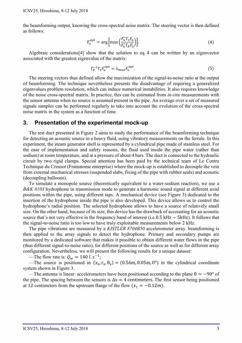
Figure 1 represents a diagram of the mock-up configuration considered in this study. The purpose

of the beamforming is to simultaneously process the sensors’ measurements (i.e. spatial filtering) to

bring out the source while rejecting the flow-induced vibration noise.

Figure 1.Schematic representation of the configuration considered to study the performance of the formation

of vibro-acoustic pathways.

2. Classical and MaxSNR beamfomring

We recall that beamforming consists of “spatially” filtering the signals registered by the antenna.

If we denote by Γ the cross-spectral matrix of the signals received by the array of sensors and by 𝐹𝑢

the steering vector (i.e. spatial filtering vector) which points at the position u of the detection space,

then the level 𝑦𝑢 at the beamforming output, is given by:

𝑦𝑢 = 𝐹𝑢∗Γ𝐹𝑢. (1)

Assuming that the signal to be detected and the noise is independent, we can decompose the matrix

Γ as such:

Γ = Γ𝑠 + Γ𝑏 , (2)

where Γ𝑠 is the cross-spectral matrix of the signals induced by the source alone and Γ𝑏 is the cross-

spectral matrix of the signals induced by the noise alone.

Assuming that the noise is homogeneous and spatially incoherent (i.e. Γ𝑏 = 𝜎𝑏𝐼) with I the identity

matrix), it can be shown that the array gain – defined as the ambiguity function maximum value for

an incoherent background noise – is maximum when the steering vector is given by:

𝐹𝑢𝑐𝑙𝑎𝑠𝑠 =

𝐻𝑢

‖𝐻𝑢‖2, (3)

where Hu is the vector containing the transfer functions between the (assumed) position u of the

source and the antenna’s accelerometers (i.e. sensors).

This beamforming technique relies on a prior knowledge of the source (through the transfer

functions) as well as on the assumption that the noise would appear spatially incoherent. This is what

will later be called the “classical” beamforming method.

However, numerical and experimental tests presented in section 4.5 show that the vibration noise

recorded by the array’s sensors (i.e. accelerometers) exhibits some spatial coherence. Inevitably, this

will lead to a deterioration in the performance of classical beamforming compared to what could be

assumed for the latter if the vibration noise showed perfect incoherence.

To overcome this obstacle, different variants of beamforming based on prior knowledge of noise

have been developed [3]. We can notably cite one that seeks to maximize the signal-to-noise ratio at

ICSV25, Hiroshima, 8-12 July 2018

ICSV25, Hiroshima, 8-12 July 2018 3

the beamforming output, knowing the cross-spectral noise matrix. The steering vector is then defined

as follows:

𝐹𝑢𝑜𝑝𝑡

= arg [max (𝐹𝑢

∗Γs𝐹𝑢

𝐹𝑢∗Γ𝑏𝐹𝑢

)]. (4)

Algebraic considerations[4] show that the solution to eq. 4 can be written by an eigenvector

associated with the greatest eigenvalue of the matrix:

Γ𝑏−1Γ𝑠𝐹𝑢

𝑜𝑝𝑡= λ𝑚𝑎𝑥𝐹𝑢

𝑜𝑝𝑡. (5)

The steering vectors thus defined allow the maximization of the signal-to-noise ratio at the output

of beamforming. The technique nevertheless presents the disadvantage of requiring a generalized

eigenvalues problem resolution, which can induce numerical instabilities. It also requires knowledge

of the noise cross-spectral matrix. In practice, this can be estimated from in-situ measurements with

the sensor antenna when no source is assumed present in the pipe. An average over a set of measured

signals samples can be performed regularly to take into account the evolution of the cross-spectral

noise matrix in the system as a function of time.

3. Presentation of the experimental mock-up

The test duct presented in Figure 2 aims to study the performance of the beamforming technique

for detecting an acoustic source in a heavy fluid, using vibratory measurements on the ferrule. In this

experiment, the steam generator shell is represented by a cylindrical pipe made of stainless steel. For

the ease of implementation and safety reasons, the fluid used inside the pipe water (rather than

sodium) at room temperature, and at a pressure of about 4 bars. The duct is connected to the hydraulic

circuit by two rigid clamps. Special attention has been paid by the technical team of Le Centre

Technique du Creusot (Framatome enterprise) where the mock-up is established to decouple the vein

from external mechanical stresses (suspended slabs, fixing of the pipe with rubber seals) and acoustic

(decoupling balloons).

To simulate a monopole source (theoretically equivalent to a water-sodium reaction), we use a

B&K 8103 hydrophone in transmission mode to generate a harmonic sound signal at different axial

positions within the pipe, using different taps. A mechanical device (see Figure 3) dedicated to the

insertion of the hydrophone inside the pipe is also developed. This device allows us to control the

hydrophone’s radial position. The selected hydrophone allows to have a source of relatively small

size. On the other hand, because of its size, this device has the drawback of accounting for an acoustic

source that’s not very effective in the frequency band of interest (i.e.0.5 kHz − 5kHz). It follows that

the signal-to-noise ratio is too low to have truly exploitable measurements below 2 kHz.

The pipe vibrations are measured by a KISTLER 8704B50 accelerometer array. beamforming is

then applied to the array signals to detect the hydrophone. Primary and secondary pumps are

monitored by a dedicated software that makes it possible to obtain different water flows in the pipe

(thus different signal-to-noise ratio), for different positions of the source as well as for different array

configuration. Nevertheless, we will present the following results for a unique dataset:

—The flow rate is: 𝑄𝑤 = 140 𝑙. 𝑠−1;

—The source is positioned in (xs, rs, θs) = (0.56m, 0.05m, 0°) in the cylindrical coordinate

system shown in Figure 3.

—The antenna is linear: accelerometers have been positioned according to the plane θ = −90° of

the pipe. The spacing between the sensors is Δx = 4 centimeters. The first sensor being positioned

at 12 centimeters from the upstream flange of the flow (𝑥1 = −0.12𝑚).

ICSV25, Hiroshima, 8-12 July 2018

ICSV25, Hiroshima, 8-12 July 2018 4

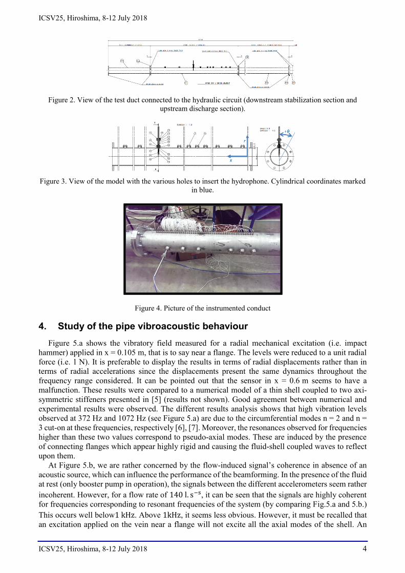
Figure 2. View of the test duct connected to the hydraulic circuit (downstream stabilization section and

upstream discharge section).

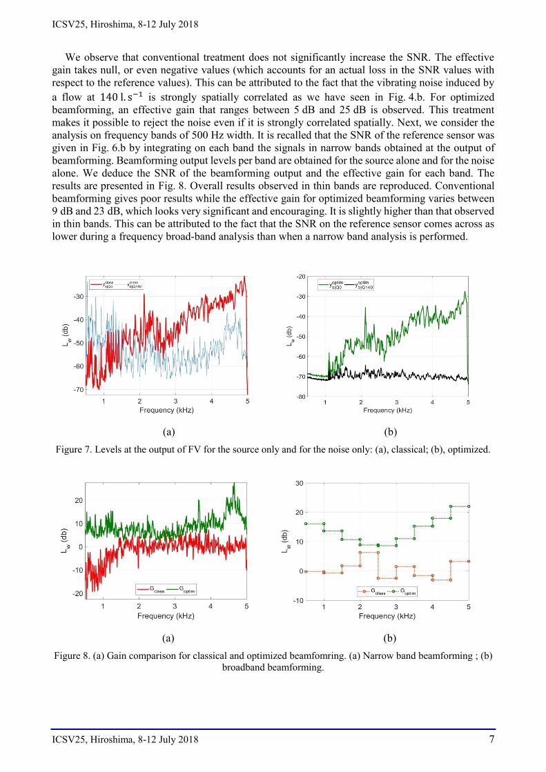
Figure 3. View of the model with the various holes to insert the hydrophone. Cylindrical coordinates marked

in blue.

Figure 4. Picture of the instrumented conduct

4. Study of the pipe vibroacoustic behaviour

Figure 5.a shows the vibratory field measured for a radial mechanical excitation (i.e. impact

hammer) applied in x = 0.105 m, that is to say near a flange. The levels were reduced to a unit radial

force (i.e. 1 N). It is preferable to display the results in terms of radial displacements rather than in

terms of radial accelerations since the displacements present the same dynamics throughout the

frequency range considered. It can be pointed out that the sensor in x = 0.6 m seems to have a

malfunction. These results were compared to a numerical model of a thin shell coupled to two axi-

symmetric stiffeners presented in [5] (results not shown). Good agreement between numerical and

experimental results were observed. The different results analysis shows that high vibration levels

observed at 372 Hz and 1072 Hz (see Figure 5.a) are due to the circumferential modes n = 2 and n =

3 cut-on at these frequencies, respectively [6], [7]. Moreover, the resonances observed for frequencies

higher than these two values correspond to pseudo-axial modes. These are induced by the presence

of connecting flanges which appear highly rigid and causing the fluid-shell coupled waves to reflect

upon them.

At Figure 5.b, we are rather concerned by the flow-induced signal’s coherence in absence of an

acoustic source, which can influence the performance of the beamforming. In the presence of the fluid

at rest (only booster pump in operation), the signals between the different accelerometers seem rather

incoherent. However, for a flow rate of 140 l. s−s, it can be seen that the signals are highly coherent

for frequencies corresponding to resonant frequencies of the system (by comparing Fig.5.a and 5.b.)

This occurs well below1 kHz. Above 1kHz, it seems less obvious. However, it must be recalled that

an excitation applied on the vein near a flange will not excite all the axial modes of the shell. An

ICSV25, Hiroshima, 8-12 July 2018

ICSV25, Hiroshima, 8-12 July 2018 5

excitation further away from the flanges would have made it possible to bring out axial modes relating

to the circumferential orders n = 0 and n = 1. Although the pressure fluctuations induced by the

turbulent flow have very weak correlations at the scale of the separation between the sensors [i.e.

4 cm], the vibration field induced by them has a strong spatial coherence at the resonance frequencies

of the system. This could be confirmed by numerical testing (see [8]).

As we will see, this strong coherence of the signals over the antenna sensors can be very damaging

for the classical beamforming.

(a) (b)

Figure 5. (a) Levels of displacement measured by the antenna sensors for mechanical excitation in x = 0.105

m. Experimental results; (b) Standardized cross-spectral matrices of accelerations between sensor # 1 and

sensor i for a flow rate Qw = 140 l. s−1.

5. Performance analysis of beamforming

5.1 Reference sensor and effective antenna gain

In order to compare the performance of beamforming techniques, it is necessary to have a reference

indicator of the pre-filtering state. For this, we will define the SNR of a sensor as the ratio of the

autospectrum of the source-to-detect induced signals in absence of any perturbing noise, to that

induced by the noise alone, in absence of all source. This means the SNR might vary from one sensor

to another. The one with the highest signal-to-noise ratio (SNR) at the frequency considered will

define the “reference” sensor.

In Fig. 5, we present the level of the SNR on the reference sensor and its number according to the

frequency. We notice that the levels on all the sensors increase with the frequency. We can observe a

general tendency of the SNR increase with frequency, which is, on the one hand, due to an increase

in the radiation of the source and, on the other hand, to a decrease in noise induced by the flow. In

addition, the reference sensor changes from one frequency to another. This definition of the SNR

reference value is only optimal for detection from a single sensor for narrow band analysis.

Nevertheless, in practice, it will not seem very relevant for the detection of broadband sources. For

broadband analysis, the SNR of a sensor is defined as the ratio of the source-induced signal level

induce alone in the band of interest, to the level of noise alone in the same band. The reference sensor

remains the one with the strongest SNR for the broadband in question. The reference SNR and

ICSV25, Hiroshima, 8-12 July 2018

ICSV25, Hiroshima, 8-12 July 2018 6

reference sensor index for 500 Hz bands are shown in Fig. 6.b. Overall, the reference SNR per band

is lower than that presented for narrow bands. The reason of this resides in the fact that reference

sensor does not change for the frequencies contained in the same frequency band.

(a) (b)

Figure 6. Signal to noise ratio and reference sensor number. (a) Narrow-band analysis; (b) Broadband

analysis

5.2 Beamforming results

Subsequently, we present the results of classical beamforming output and MaxSNR beamforming

with steering vectors defined from equations (3) and (5), respectively. The transfer functions Hu

between the sensors and the source involved in the definition of these steering vectors have been

obtained experimentally from acquisitions in the presence of a source without water flow. We recall

that, given the size of the hydrophone, the coherence between the signal of the source and the signals

received by the antenna appears rather weak for the frequencies between 500 Hz and 2 kHz. We will

therefore consider the results below 2 kHz with caution. For optimized beamforming, we consider

the cross-spectral matrix of signals between the sensors in the absence of the source for the flow rate

considered (140 l. s−1).

5.2.1 Narrow and broadband investigation

Beamforming is applied for the hydrophone signal without water flow in the mock-up, as well as

for the non-signaling flow noise signal. We illustrate in Fig. 7 the output levels of classical and

optimized beamforming for the case where there is only the source to detect (i.e. source with a zero

flow) or where there is only noise (i.e. no source with a flow rate of 140 l / s). It can be seen that the

differences between the signal output levels of the signal and the noise appear generally greater for

optimized beamforming than for the conventional one. These differences are mainly due to the fact

that the output level of beamforming for the noise is lowered by the optimized treatment with respect

to the conventional treatment. Optimized processing seems better at rejecting noise than conventional

processing (which results from its definition).

From the previous results, we can calculate the SNR at the output of beamforming. By substracting

with the SNR on the reference sensor, we obtain the effective antenna gain for the 2 treatments. The

results are shown in Fig. 8.

ICSV25, Hiroshima, 8-12 July 2018

ICSV25, Hiroshima, 8-12 July 2018 7

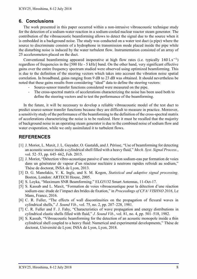
We observe that conventional treatment does not significantly increase the SNR. The effective

gain takes null, or even negative values (which accounts for an actual loss in the SNR values with

respect to the reference values). This can be attributed to the fact that the vibrating noise induced by

a flow at 140 l. s−1 is strongly spatially correlated as we have seen in Fig. 4.b. For optimized

beamforming, an effective gain that ranges between 5 dB and 25 dB is observed. This treatment

makes it possible to reject the noise even if it is strongly correlated spatially. Next, we consider the

analysis on frequency bands of 500 Hz width. It is recalled that the SNR of the reference sensor was

given in Fig. 6.b by integrating on each band the signals in narrow bands obtained at the output of

beamforming. Beamforming output levels per band are obtained for the source alone and for the noise

alone. We deduce the SNR of the beamforming output and the effective gain for each band. The

results are presented in Fig. 8. Overall results observed in thin bands are reproduced. Conventional

beamforming gives poor results while the effective gain for optimized beamforming varies between

9 dB and 23 dB, which looks very significant and encouraging. It is slightly higher than that observed

in thin bands. This can be attributed to the fact that the SNR on the reference sensor comes across as

lower during a frequency broad-band analysis than when a narrow band analysis is performed.

(a) (b)

Figure 7. Levels at the output of FV for the source only and for the noise only: (a), classical; (b), optimized.

(a) (b)

Figure 8. (a) Gain comparison for classical and optimized beamfomring. (a) Narrow band beamforming ; (b)

broadband beamforming.

ICSV25, Hiroshima, 8-12 July 2018

ICSV25, Hiroshima, 8-12 July 2018 8

6. Conclusions

The work presented in this paper occurred within a non-intrusive vibroacoustic technique study

for the detection of a sodium-water reaction in a sodium-cooled nuclear reactor steam generator. The

contribution of the vibroacoustic beamforming allows to detect the signal due to the source when it

is embedded in a background noise. The study was conducted on a water test duct (a pipe) where the

source to discriminate consists of a hydrophone in transmission mode placed inside the pipe while

the disturbing noise is induced by the water turbulent flow. Instrumentation consisted of an array of

25 accelerometers placed on the duct.

Conventional beamforming appeared inoperative at high flow rates (i.e. typically 140 l. s−1)

regardless of frequencies in the [500 Hz - 5 kHz] band. On the other hand, very significant effective

gains over the entire frequency spectrum studied were observed using optimized beamforming. This

is due to the definition of the steering vectors which takes into account the vibration noise spatial

correlation. In broadband, gains ranging from 9 dB to 23 dB was obtained. It should nevertheless be

noted that these gains results from considering “ideal” data to define the steering vectors:

- Source-sensor transfer functions considered were measured on the pipe.

- The cross-spectral matrix of accelerations characterizing the noise has been used both to

define the steering vectors and to test the performance of the beamforming.

In the future, it will be necessary to develop a reliable vibroacoustic model of the test duct to

predict source-sensor transfer functions because they are difficult to measure in practice. Moreover,

a sensitivity study of the performance of the beamforming to the definition of the cross-spectral matrix

of accelerations characterizing the noise is to be realized. Here it must be recalled that the majority

of background noise in an operating steam generator is due to the combined noise of sodium flow and

water evaporation, while we only assimilated it to turbulent flows.

REFERENCES

[1] J. Moriot, L. Maxit, J. L. Guyader, O. Gastaldi, and J. Périsse, “Use of beamforming for detecting

an acoustic source inside a cylindrical shell filled with a heavy fluid,” Mech. Syst. Signal Process.,

vol. 52–53, pp. 645–662, Feb. 2015.

[2] J. Moriot, “Détection vibro-acoustique passive d’une réaction sodium-eau par formation de voies

dans un générateur de vapeur d’un réacteur nucléaire à neutrons rapides refroidi au sodium,”

Thèse de doctorat, INSA de Lyon, 2013.

[3] D. G. Manolakis, V. K. Ingle, and S. M. Kogon, Statistical and adaptive signal processing.

Boston, London: ARTECH House, 2005.

[4] S. Loyka, “Maximum SNR Beamforming.” ELG5132 Smart Antennas, 11-Oct-17.

[5] S. Kassab and L. Maxit, “Formation de voies vibroacoustique pour la détection d’une réaction

sodium-eau: étude de l’impact des brides de fixation,” in Proceedings of CFA/ VISHNO 2016, Le

Mans, France, 2016.

[6] C. R. Fuller, “The effects of wall discontinuities on the propagation of flexural waves in

cylindrical shells,” J. Sound Vib., vol. 75, no. 2, pp. 207–228, 1981.

[7] C. R. Fuller and F. J. Fahy, “Characteristics of wave propagation and energy distributions in

cylindrical elastic shells filled with fluid,” J. Sound Vib., vol. 81, no. 4, pp. 501–518, 1982.

[8] S. Kassab, “Vibroacoustic beamforming for the detection of an acoustic monopole inside a thin

cylindrical shell coupled to a heavy fluid: Numerical and experimental developments,” Thèse de

doctorat, Université de Lyon; INSA de Lyon, Lyon, 2018.