Detecting Small-Scale Variability of Trace Elements in a Shallow Aquifer

1

Detecting small scale variability of trace elements in a shallow aquifer 1

2

Beatrice M. S. Giambastiani1, Nicolò Colombani

2, Micòl Mastrocicco

3# 3

4 1 Interdepartmental Research Centre for Environmental Sciences (CIRSA), University of Bologna, Via S. Alberto 163, 5

48123 Ravenna, Italy 6 2 Department of Earth Sciences, “Sapienza” University, P.le A. Moro 5, 00185 Rome, Italy 7 3 Department of Physics and Earth Sciences, University of Ferrara, Via Saragat 1, 44122 Ferrara, Italy 8 # corresponding author: [email protected] 9

Ph: +39 0532 974692 10

Fax: +39 0532 974767 11

12

Abstract 13

14

Groundwater samples collected from an unconfined shallow aquifer were analysed for major and trace elements (TEs) 15

concentrations with the aim to investigate small scale variations possibly linked to fertilizer residual products applied 16

until 2004. The field site, located near Ferrara (Northern Italy), covers an area of 200 m2 and was a former agricultural 17

field then converted into park and equipped with a grid of 13 monitoring wells. Three monitoring campaigns were 18

carried out in June 2007, March and June 2009 in order to detect spatial and temporal variations in water quality. 19

Groundwater nitrate, chloride, bromide and sulphate concentrations decreased with time indicating that the fertilizer 20

plume was slowly replaced by unpolluted groundwater. However, the groundwater composition showed values of TEs 21

above the recommended international and national guideline values. Dissolved TEs concentrations varied randomly in 22

the three campaigns, while TEs in the solid matrix did not show particular enrichment factors induced by fertilizer use. 23

The data indicated that the dominant factor involved in determining small scale spatial variability of TEs concentrations 24

in this shallow aquifer was the sediment-water interaction, while the temporal variation of TEs was driven by the 25

organic matter leaching from the topsoil and by water table oscillations, which in turn drove the groundwater redox 26

status. 27

This study emphasizes the need of small scale TEs spatial resolution to discriminate between anthropogenic non-point 28

sources of pollution (like fertilizers) and background concentrations. 29

30

Key words trace elements; groundwater quality; fertilizers; shallow aquifer; monitoring. 31

32

INTRODUCTION 33

34

Groundwater quality depends on several natural factors (i.e. aquifer lithology, recharge water, ground and surface water 35

interactions, etc.) but also on human activities (i.e. fertilization), which can alter the groundwater quality (Stark and 36

Richards 2008). 37

Nitrate leaching to groundwater from fertilizers has been object of many studies in the last years throughout the world 38

(Gehl et al. 2002; Köhler et al. 2006; Ibendahl and Fleming 2007; McMahon et al. 2008; Perego et al. 2012) and it can 39

be considered a major source of non-point pollution in soils and waters (Galloway et al. 2008). To protect these 40

2

vulnerable resources, threshold values have been adopted in groundwater and in water intended for human 1

consumptions (EU Directive 1998; U.S. EPA 2003; 2009). 2

Despite the large literature on groundwater nitrate pollution from fertilizers, much less has been done on heavy metals 3

and trace elements (TEs) in groundwater bodies beneath agricultural fields. Some comprehensive works on fertilizers 4

characterization (Abdel-Haleem et al. 2001; Otero et al. 2005) give detailed information about the potential leaching of 5

TEs to groundwater and surface waters. However, few are the documented field studies on groundwater contamination 6

from TEs derived from fertilizers application. Usually the studies on TEs of agrochemical origin addressed the problem 7

using regional statistical approaches (Helena et al. 2000; Nouri et al. 2008; Wongsasuluk et al. 2014), or more often 8

focus on soil contamination and biomonitoring (Zhao et al. 2010). 9

Nevertheless, to quantify whether groundwater contamination with TEs is imputable to a diffuse source of pollution 10

(like fertilizers), point sources (sewers or chemical plants) or geogenic sources is not straightforward, given that the 11

concentration of TEs varies accordingly to pH and redox state of the water-matrix continuum (Appelo and Postma 12

2005). In fact, the spatial and temporal variability of concentrations can be significant at small scales, posing problems 13

to directly relate the concentration in groundwater with possible sources of contaminations. 14

To elucidate this key factor, the current study reports the temporal and spatial variation of major ions and TEs in a 15

shallow unconfined aquifer. A 200 m2 field is equipped with a relatively dense monitoring network, consisting of 13 16

monitoring wells 5 m spaced. Groundwater and sediment samples were collected in order to characterize both the 17

aqueous and solid phases constituting the unconfined aquifer. Three sampling companies were performed in June 2007, 18

March 2009 and June 2009 to capture groundwater quality variations induced by land use change from agricultural land 19

to park. The main aim of this work is to explain the causes of the spatial and temporal variability detected in 20

groundwater at a metric scale. 21

22

MATERIALS AND METHODS 23

24

Site description 25

26 The study site is located in a former agricultural field overlying a river paleochannel near Ferrara, in the Po River plain 27

(Northern Italy) (Figure 1). This area was cultivated with cereal rotation from 1986 to 2004 using urea at an average 28

rate of 300 kg/ha/year. In 2004 the field was converted into a park with grass cover (experimental field site) and no 29

more fertilized nor treated with pesticides. 30

13 monitoring wells were installed in June 2007 and monitored 3 times (June 2007, March and June 2009) for 31

groundwater quality and head distribution. All monitoring wells are 5-10 cm in inner diameter and are fully screened 32

from 1 to 8 m below ground level (b.g.l.). The monitoring wells are installed in the unconfined aquifer hosted by the 33

paleochannel, which is composed of Holocenic fluvial sandy deposits with clay and silt lenses (5 m thick). The 34

underlying confining unit (10 m in thick), consists of impermeable clay and silt sediments rich in organic matter and 35

peat (lithological cross section in Figure 1). The latter sediments have been deposited in freshwater marsh and lagoon 36

environments, in a period of water stagnation following a rapid sea level rise at the beginning of the present interglacial 37

age (Amorosi et al. 1999); 18 m b.g.l. a 25 m thick succession of Würmian fluvial deposits (sand with sparse clay and 38

silt lenses) hosts the confined aquifer. Geological setting of the area reflects the Late Quaternary succession of marginal 39

marine and continental sediments formed under a predominantly glacio-eustatic control (Amorosi et al. 1999). 40

41

3

1

Figure 1. In the upper panel are shown piezometric contour (m a.s.l.) (cyan lines), groundwater directions (cyan 2

arrows), location of shallow groundwater wells (cyan diamonds), principal canals (blue lines), surface water sampling 3

point (red dot), the septic tanks (red dashed polygons) and the field site (red square). In the middle panel are shown the 4

13 monitoring wells, local hydraulic head contours (m a.s.l.) and paleochannel boundaries. In the lower panel is also 5

shown the paleochannel reconstruction along the transect AB (as inferred from core logs, geomorphologic and ERT 6

surveys by Mastrocicco et al. 2010). 7

8

Detailed sedimentological, geochemical and mineralogical analyses of the Late Quaternary deposits of the Po River 9

plain are discussed in Amorosi et al. (2002). Alluvial sediments of the Po River are characterized by elevated 10

background values of Cr and Ni that represent a natural geochemical anomaly. Comacchio and Ferrara areas are 11

characterized by a sharp increase in Cr/Al2O3 and serpentine/silicate ratios, reflecting the general shift from an 12

Apenninic source area, which represented the major feeding area at lowstand time and early stages of transgression, to a 13

Po River-derived source area (mix of Apenninic and Alpine deposits), which acted as the major source of sediment 14

during the late transgressive and highstand phases. The north-eastern hydraulic gradient of the shallow unconfined 15

aquifer (1-3‰, Figure 1) is manly controlled by canals and drains. The mean groundwater level is 2.5 m a.s.l. over the 16

4

year, with an average seasonal variation of 0.5 m (Mastrocicco et al. 2011). The groundwater has nearly constant 1

electrical conductivity around 1±0.1 mS/cm. The average hydraulic conductivity, based on in situ multi-level slug tests, 2

is 7.7*10-5 m/s (Mastrocicco et al. 2010), which gives an average groundwater velocity of 5±3 cm/day, applying the 3

Darcy law with an effective porosity of 0.25. In the saturated zone, the mechanical dispersion tensor was well described 4

by single lumped values for the whole site (0.53, 0.053 and 0.0053 m for longitudinal, transversal and vertical 5

dispersivity, respectively) using the numerical model MT3DMS calibrated versus dissolved Cl- concentrations 6

(Mastrocicco et al. 2011). These low values suggest a relatively homogenous transport of solutes in the saturated zone 7

dominated by advection. The recharge could be assumed spatially homogeneous, although its temporal distribution 8

during 2007-2009 period was not homogenous based on the results of HYDRUS-1D modelling (Mastrocicco et al. 9

2011) and the time taken by non-reactive dissolved species to reach the water table was between 1 and 4 months, 10

according to the moisture condition of the unsaturated zone. 11

12

Water samples and analyses 13

14

The 13 monitoring wells in the field site were monitored in order to detect variations in groundwater quality and head 15

distribution. 16

Groundwater level, electrical conductivity and temperature were monitored by Solinst levelogger, while dissolved 17

oxygen (DO), pH and Eh measurements were taken by HANNA multi parameters probe. 18

Groundwater samples were collected 2 m below the water table (about 1 m a.s.l.) in each monitoring well via the 800 L 19

straddle packers system (Solinst, Canada) with a sampling window of 0.2 m. The samples were collected via a low-flow 20

technique using an inertial pump after purging of about 5 L. This technique permits to collect groundwater samples at a 21

specific depth by isolating a portion of the aquifer and avoiding water mixing during the sampling (Mastrocicco et al. 22

2012). The collected groundwater samples were filtered through 0.22 µm Dionex polypropylene filters, stored in a cool 23

box at 4°C, immediately transported at the Hydrochemistry Laboratory of the University of Ferrara and analysed for the 24

major ions using an isocratic dual pump ion chromatography ICS-1000 Dionex. An AS-40 Dionex auto-sampler was 25

employed to run the analyses. Quality Control (QC) with standard samples was run every 10 samples and the standard 26

deviation for all QC samples was better than 4%. 27

Samples for TEs analysis were collected in acid-washed Nalgene bottles, preserved with ultra-trace 0.2 N HCl and 28

stored at 4 °C until analysed at the Geochemistry Laboratory of the University of Ferrara. TEs in groundwater (Al, Mn, 29

Fe, As, Hg, B, Ba, U, Li, Be, V, Cr, Co, Ni, Cu, Zn, Ga, Rb, Mo, Cd, Sb, Te, Tl, Bi) were analysed using an X Series 30

Thermo-Scientific spectrometer (ICP-MS). Specific amounts of Rh, In and Re were added to the analysed solutions as 31

an internal standard, in order to correct for instrumental drift. Accuracy and precision, based on replicated analyses of 32

samples and standards, are better than 10% for all elements, well above the detection limit of 0.01 µg/L. The E.P.A. 33

Reference Standard SS-1 (a Type B naturally contaminated soil) and the E.P.A. Reference Standard SS-2 (a Type C 34

naturally contaminated soil) were also analysed to cross-check and validate the results. 35

Surface water samples, collected from the canal near the field site (upper panel in Figure 1) in each monitoring 36

campaign, together with rainfall samples collected in 2007 from a rain bucket placed on the field, were also analysed for 37

the same major and trace elements. 38

To characterize the water-soluble fraction of the fertilizer (urea) used on the field site from 1986 to 2004, 1 g of 39

fertiliser was dissolved both in 250 ml and 100 ml of distilled water, stirred for 24 h and filtered with a Millipore®

filter 40

5

of 0.45 lm pore size. The major ions concentrations were taken using 1:250 solid:liquid ratio, while 1:100 solid:liquid 1

ratio was used to measure the TEs concentrations. 2

3

Sediment samples and analyses 4

5

In June 2007, sediment samples were collected every 0.5 m (from 0 to -4 m b.g.l) via auger hole drilling in P1, near the 6

monitoring well C4 (Figure 1). All samples were completely oven dried at 50°C, powdered, homogenized in an agate 7

mortar and analysed by X-ray fluorescence (XRF) on powder pellets, using a wavelength-dispersive automated ARL 8

Advant’X spectrometer. Accuracy and precision based on systematic re-analysis of standards were better than 3% for 9

major oxides (SiO2, TiO2, Al2O3, Fe2O3, MnO, MgO, CaO, Na2O, K2O and P2O5), while accuracy and precision were 10

below 10% for TEs (Ba, Ce, Co, Cr, La, Nb, Ni, Pb, Rb, Sr, Th, V, Y, Zn, Zr, Cu, Ga, Nd and Sc). The detection limit 11

for TEs was 3 ppm. Loss on Ignition (LOI) was evaluated after overnight heating at 950°C (LOI950) in order to represent 12

measure (wt%) of volatile substances such as pore water, inorganic carbon and organic matter. The sediment organic 13

matter (SOM) content was measured by dry combustion (Tiessen and Moir 1993). 14

15

RESULTS AND DISCUSSION 16

17

Major ions in groundwater 18

Figure 2 shows the relationship between chloride (Cl-) and bromide (Br-) concentrations in water samples from the three 19

monitoring campaigns. Br- and Cl- are non-reactive ions because their content is neither influenced by redox processes, 20

nor controlled by minerals precipitation-dissolution and sorption (Davis et al. 1998): if Cl- and Br- have a single origin 21

(i.e. actual seawater), the Cl-/Br- ratio must remain constant. Cl-/Br- ratios greater than 300 can be directly related to 22

sources of Cl- other than atmospheric deposition. Br- and Cl- ions and their ratios can be used as tracer to distinguish 23

between natural and anthropogenic sources of contamination, such as sewage effluent (Vengosh and Pankratov 1998), 24

septic systems and fertilizers (Katz et al. 2011). 25

26

Figure 2. Plot of Cl-/Br- molar ratio vs. Cl- (mg/l) in the groundwater samples. Reported are also Cl-/Br- molar ratios of 27

the local precipitation, canal freshwater and fertilizer. 28

6

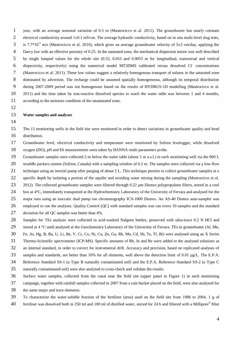
Major ions and TEs concentrations of the urea fertilizer, used until 2004 on the field, are reported in Table 1. 1

2

Table 1. Major ions and TEs concentrations (ppm) analysed in the water-soluble fraction of the urea fertilizer. 3

Urea fertilizer (ppm)

F- Cl

- NO2

- Br

- NO3

- PO4

3-

1.82 405.22 < 0.1 1.18 4.39 400.24

SO42-

Li Be B Na Mg

737.58 0.02 3.3E-05 1.67 552.70 135.29

Al K Ca Ti V Cr

0.40 1807.13 43.73 0.43 0.05 0.07

Mn Fe Co Ni Cu Zn

0.17 0.30 0.05 0.18 0.18 1.05

Ga As Se Rb Sr Mo

4.94E-03 0.02 0.05 0.56 0.14 0.06

Ag Cd Sn Sb Te Ba

< 0.001 5.80E-04 1.27E-03 3.32E-03 1.69E-03 0.02

Hg Tl Pb Bi U

8.67E-04 6.07E-04 2.54E-03 < 0.001 3.40E-03

4

The fertilizer has a Cl-/Br- molar ratio equal to 774±52. Several groundwater samples from the campaign of June 2007 5

are depleted in Br- and plot along or above the fertilizer Cl-/Br- molar ratio with an average value of 738 and a 6

maximum value of 1228 (Figure 2), testifying the input of recharge water reach in fertilizers. Groundwater samples 7

from the campaigns of March and June 2009 have Cl-/Br- molar ratios ranging from 264 to 569 indicating a further 8

dilution of fertilizers. These samples show variable concentration of Br- and a nearly constant concentration of Cl- 9

suggesting a possible mixing between rainfall and canal water. The latter shows variable concentrations of Cl- and other 10

dissolved species over time (Table 2). In particular, major ions peaked in March 2009 in correspondence with the 11

maximum drainage from the agricultural fields aligned along the canal. 12

13

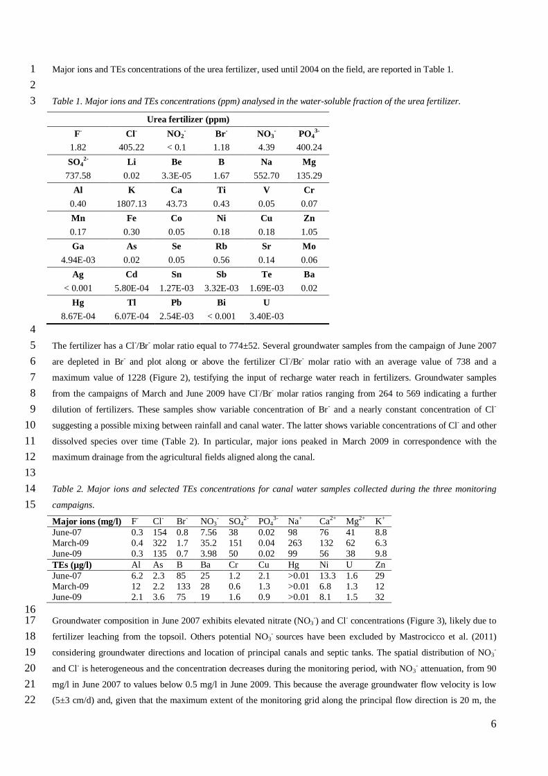
Table 2. Major ions and selected TEs concentrations for canal water samples collected during the three monitoring 14

campaigns. 15

Major ions (mg/l) F- Cl- Br- NO3- SO4

2- PO43- Na+ Ca2+ Mg2+ K+

June-07 0.3 154 0.8 7.56 38 0.02 98 76 41 8.8

March-09 0.4 322 1.7 35.2 151 0.04 263 132 62 6.3

June-09 0.3 135 0.7 3.98 50 0.02 99 56 38 9.8

TEs (µg/l) Al As B Ba Cr Cu Hg Ni U Zn

June-07 6.2 2.3 85 25 1.2 2.1 >0.01 13.3 1.6 29

March-09 12 2.2 133 28 0.6 1.3 >0.01 6.8 1.3 12

June-09 2.1 3.6 75 19 1.6 0.9 >0.01 8.1 1.5 32

16 Groundwater composition in June 2007 exhibits elevated nitrate (NO3

-) and Cl- concentrations (Figure 3), likely due to 17

fertilizer leaching from the topsoil. Others potential NO3- sources have been excluded by Mastrocicco et al. (2011) 18

considering groundwater directions and location of principal canals and septic tanks. The spatial distribution of NO3- 19

and Cl- is heterogeneous and the concentration decreases during the monitoring period, with NO3- attenuation, from 90 20

mg/l in June 2007 to values below 0.5 mg/l in June 2009. This because the average groundwater flow velocity is low 21

(5±3 cm/d) and, given that the maximum extent of the monitoring grid along the principal flow direction is 20 m, the 22

7

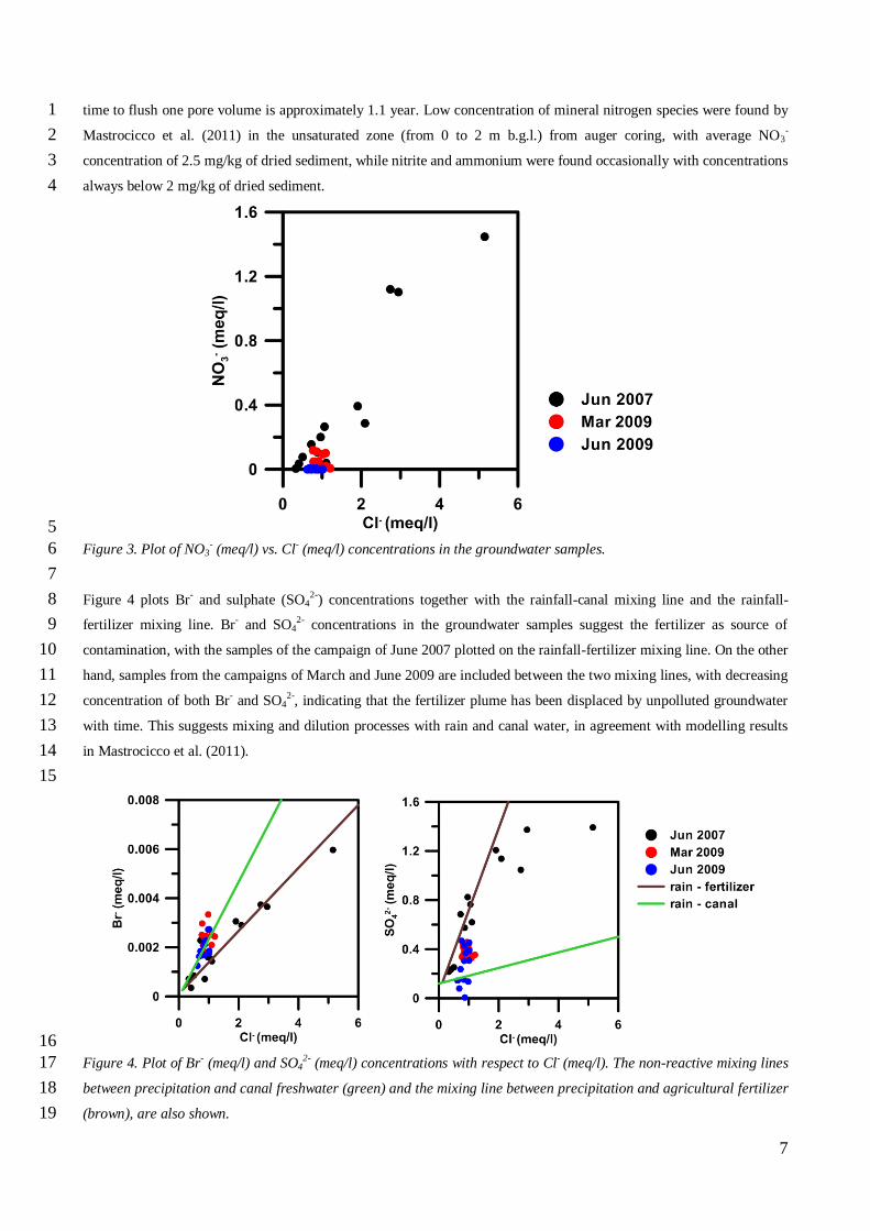
time to flush one pore volume is approximately 1.1 year. Low concentration of mineral nitrogen species were found by 1

Mastrocicco et al. (2011) in the unsaturated zone (from 0 to 2 m b.g.l.) from auger coring, with average NO3- 2

concentration of 2.5 mg/kg of dried sediment, while nitrite and ammonium were found occasionally with concentrations 3

always below 2 mg/kg of dried sediment. 4

5

Figure 3. Plot of NO3- (meq/l) vs. Cl- (meq/l) concentrations in the groundwater samples. 6

7

Figure 4 plots Br- and sulphate (SO42-) concentrations together with the rainfall-canal mixing line and the rainfall-8

fertilizer mixing line. Br- and SO42- concentrations in the groundwater samples suggest the fertilizer as source of 9

contamination, with the samples of the campaign of June 2007 plotted on the rainfall-fertilizer mixing line. On the other 10

hand, samples from the campaigns of March and June 2009 are included between the two mixing lines, with decreasing 11

concentration of both Br- and SO42-, indicating that the fertilizer plume has been displaced by unpolluted groundwater 12

with time. This suggests mixing and dilution processes with rain and canal water, in agreement with modelling results 13

in Mastrocicco et al. (2011). 14

15

16

Figure 4. Plot of Br- (meq/l) and SO42- (meq/l) concentrations with respect to Cl- (meq/l). The non-reactive mixing lines 17

between precipitation and canal freshwater (green) and the mixing line between precipitation and agricultural fertilizer 18

(brown), are also shown. 19

8

1

TEs in groundwater 2

Even if the fertilizer plume (NO3- and SO4

2-) has been flushed downstream over the monitoring grid by continuous 3

displacement driven by canal water, groundwater composition in 2009 still shows values of some TEs above the 4

national and international threshold values (Figure 5): Italian (D.L. 31/2001) and European normative limits for 5

drinking water (EU Directive 1998), U.S. Environmental Protection Agency (EPA 2009) and World Health 6

Organization (WHO) guidelines (WHO 1996; 2008). 7

Figure 5 shows concentrations of Fe, Mn, Al, As, Hg, B, Ba and U in the groundwater samples while the other TEs 8

concentrations are reported in Table 3. Since the average analytical error for all the TEs was within 10%, from both 9

Figure 5 and Table 3 is evident that for most of the TEs the analytical variability was much lower than the temporal 10

variability. In particular, the concentrations of Fe, Al, Mg and U spanned over at least 2 orders of magnitude, the 11

concentrations of As, Hg, Bo, Ba, V, Cr, Ni, Cu, Zn, Mo, Cd, Sb, Te, Tl and Bi spanned over at least 1 order of 12

magnitude, while Li, Be, Co, Ga and Rb were the only TEs showing a temporal variability in the range of the analytical 13

variability. Table 4 lists background TEs concentrations available from ARPA (Environmental Protection Agency of 14

Emilia-Romagna Region) database for the unconfined aquifer of the Ferrara province (unpublished data). Data refer to 15

long term monitoring (1997-2012) from unpolluted monitoring wells disseminated throughout the Ferrara province. 16

Only few TEs are available from this dataset to reconstruct reliable background values. 17

18

Figure 5. Upper panels: redox potential (mV) and groundwater head values (m a.s.l.) of the three campaigns. (Note: 19

lines are merely added to help the visualization). Lower panels: plots of the spatial variability of DOC in the three 20

sampling campaigns 21

9

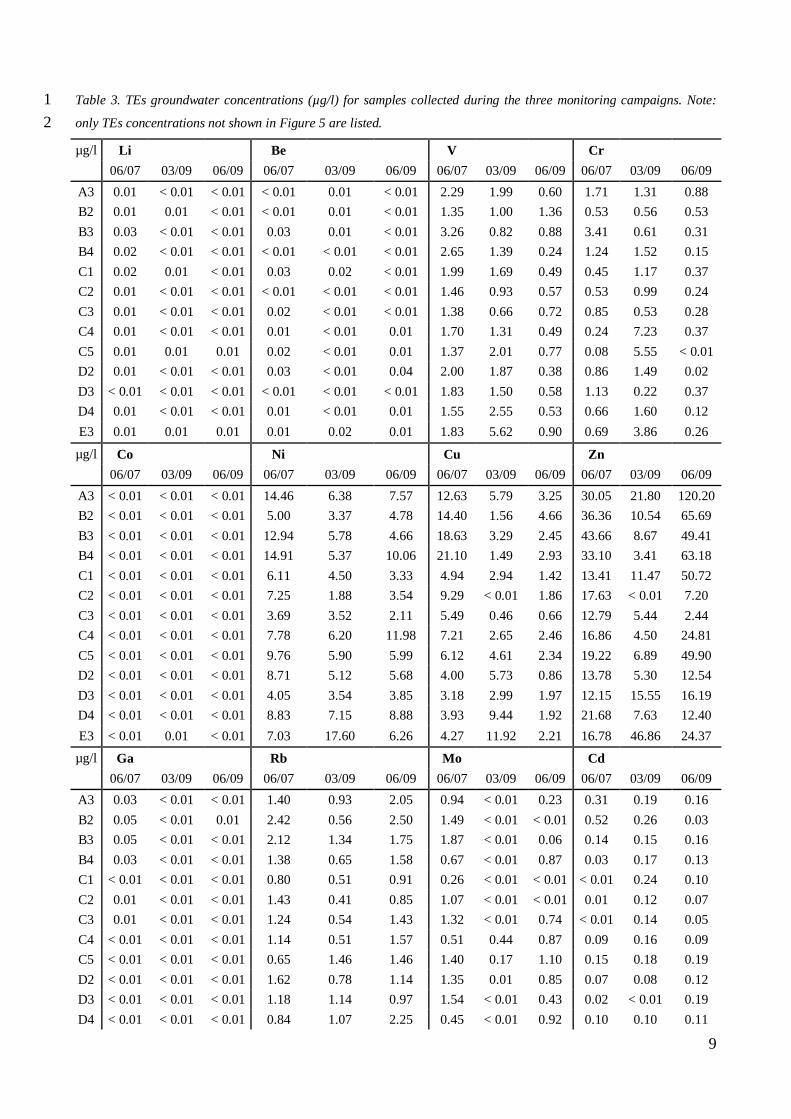
Table 3. TEs groundwater concentrations (µg/l) for samples collected during the three monitoring campaigns. Note: 1

only TEs concentrations not shown in Figure 5 are listed. 2

µg/l Li

Be

V

Cr

06/07 03/09 06/09 06/07 03/09 06/09 06/07 03/09 06/09 06/07 03/09 06/09

A3 0.01 < 0.01 < 0.01 < 0.01 0.01 < 0.01 2.29 1.99 0.60 1.71 1.31 0.88

B2 0.01 0.01 < 0.01 < 0.01 0.01 < 0.01 1.35 1.00 1.36 0.53 0.56 0.53

B3 0.03 < 0.01 < 0.01 0.03 0.01 < 0.01 3.26 0.82 0.88 3.41 0.61 0.31

B4 0.02 < 0.01 < 0.01 < 0.01 < 0.01 < 0.01 2.65 1.39 0.24 1.24 1.52 0.15

C1 0.02 0.01 < 0.01 0.03 0.02 < 0.01 1.99 1.69 0.49 0.45 1.17 0.37

C2 0.01 < 0.01 < 0.01 < 0.01 < 0.01 < 0.01 1.46 0.93 0.57 0.53 0.99 0.24

C3 0.01 < 0.01 < 0.01 0.02 < 0.01 < 0.01 1.38 0.66 0.72 0.85 0.53 0.28

C4 0.01 < 0.01 < 0.01 0.01 < 0.01 0.01 1.70 1.31 0.49 0.24 7.23 0.37

C5 0.01 0.01 0.01 0.02 < 0.01 0.01 1.37 2.01 0.77 0.08 5.55 < 0.01

D2 0.01 < 0.01 < 0.01 0.03 < 0.01 0.04 2.00 1.87 0.38 0.86 1.49 0.02

D3 < 0.01 < 0.01 < 0.01 < 0.01 < 0.01 < 0.01 1.83 1.50 0.58 1.13 0.22 0.37

D4 0.01 < 0.01 < 0.01 0.01 < 0.01 0.01 1.55 2.55 0.53 0.66 1.60 0.12

E3 0.01 0.01 0.01 0.01 0.02 0.01 1.83 5.62 0.90 0.69 3.86 0.26

µg/l Co

Ni

Cu

Zn

06/07 03/09 06/09 06/07 03/09 06/09 06/07 03/09 06/09 06/07 03/09 06/09

A3 < 0.01 < 0.01 < 0.01 14.46 6.38 7.57 12.63 5.79 3.25 30.05 21.80 120.20

B2 < 0.01 < 0.01 < 0.01 5.00 3.37 4.78 14.40 1.56 4.66 36.36 10.54 65.69

B3 < 0.01 < 0.01 < 0.01 12.94 5.78 4.66 18.63 3.29 2.45 43.66 8.67 49.41

B4 < 0.01 < 0.01 < 0.01 14.91 5.37 10.06 21.10 1.49 2.93 33.10 3.41 63.18

C1 < 0.01 < 0.01 < 0.01 6.11 4.50 3.33 4.94 2.94 1.42 13.41 11.47 50.72

C2 < 0.01 < 0.01 < 0.01 7.25 1.88 3.54 9.29 < 0.01 1.86 17.63 < 0.01 7.20

C3 < 0.01 < 0.01 < 0.01 3.69 3.52 2.11 5.49 0.46 0.66 12.79 5.44 2.44

C4 < 0.01 < 0.01 < 0.01 7.78 6.20 11.98 7.21 2.65 2.46 16.86 4.50 24.81

C5 < 0.01 < 0.01 < 0.01 9.76 5.90 5.99 6.12 4.61 2.34 19.22 6.89 49.90

D2 < 0.01 < 0.01 < 0.01 8.71 5.12 5.68 4.00 5.73 0.86 13.78 5.30 12.54

D3 < 0.01 < 0.01 < 0.01 4.05 3.54 3.85 3.18 2.99 1.97 12.15 15.55 16.19

D4 < 0.01 < 0.01 < 0.01 8.83 7.15 8.88 3.93 9.44 1.92 21.68 7.63 12.40

E3 < 0.01 0.01 < 0.01 7.03 17.60 6.26 4.27 11.92 2.21 16.78 46.86 24.37

µg/l Ga

Rb

Mo

Cd

06/07 03/09 06/09 06/07 03/09 06/09 06/07 03/09 06/09 06/07 03/09 06/09

A3 0.03 < 0.01 < 0.01 1.40 0.93 2.05 0.94 < 0.01 0.23 0.31 0.19 0.16

B2 0.05 < 0.01 0.01 2.42 0.56 2.50 1.49 < 0.01 < 0.01 0.52 0.26 0.03

B3 0.05 < 0.01 < 0.01 2.12 1.34 1.75 1.87 < 0.01 0.06 0.14 0.15 0.16

B4 0.03 < 0.01 < 0.01 1.38 0.65 1.58 0.67 < 0.01 0.87 0.03 0.17 0.13

C1 < 0.01 < 0.01 < 0.01 0.80 0.51 0.91 0.26 < 0.01 < 0.01 < 0.01 0.24 0.10

C2 0.01 < 0.01 < 0.01 1.43 0.41 0.85 1.07 < 0.01 < 0.01 0.01 0.12 0.07

C3 0.01 < 0.01 < 0.01 1.24 0.54 1.43 1.32 < 0.01 0.74 < 0.01 0.14 0.05

C4 < 0.01 < 0.01 < 0.01 1.14 0.51 1.57 0.51 0.44 0.87 0.09 0.16 0.09

C5 < 0.01 < 0.01 < 0.01 0.65 1.46 1.46 1.40 0.17 1.10 0.15 0.18 0.19

D2 < 0.01 < 0.01 < 0.01 1.62 0.78 1.14 1.35 0.01 0.85 0.07 0.08 0.12

D3 < 0.01 < 0.01 < 0.01 1.18 1.14 0.97 1.54 < 0.01 0.43 0.02 < 0.01 0.19

D4 < 0.01 < 0.01 < 0.01 0.84 1.07 2.25 0.45 < 0.01 0.92 0.10 0.10 0.11

10

E3 < 0.01 0.01 < 0.01 0.58 1.90 1.57 0.41 < 0.01 0.56 0.38 0.24 0.17

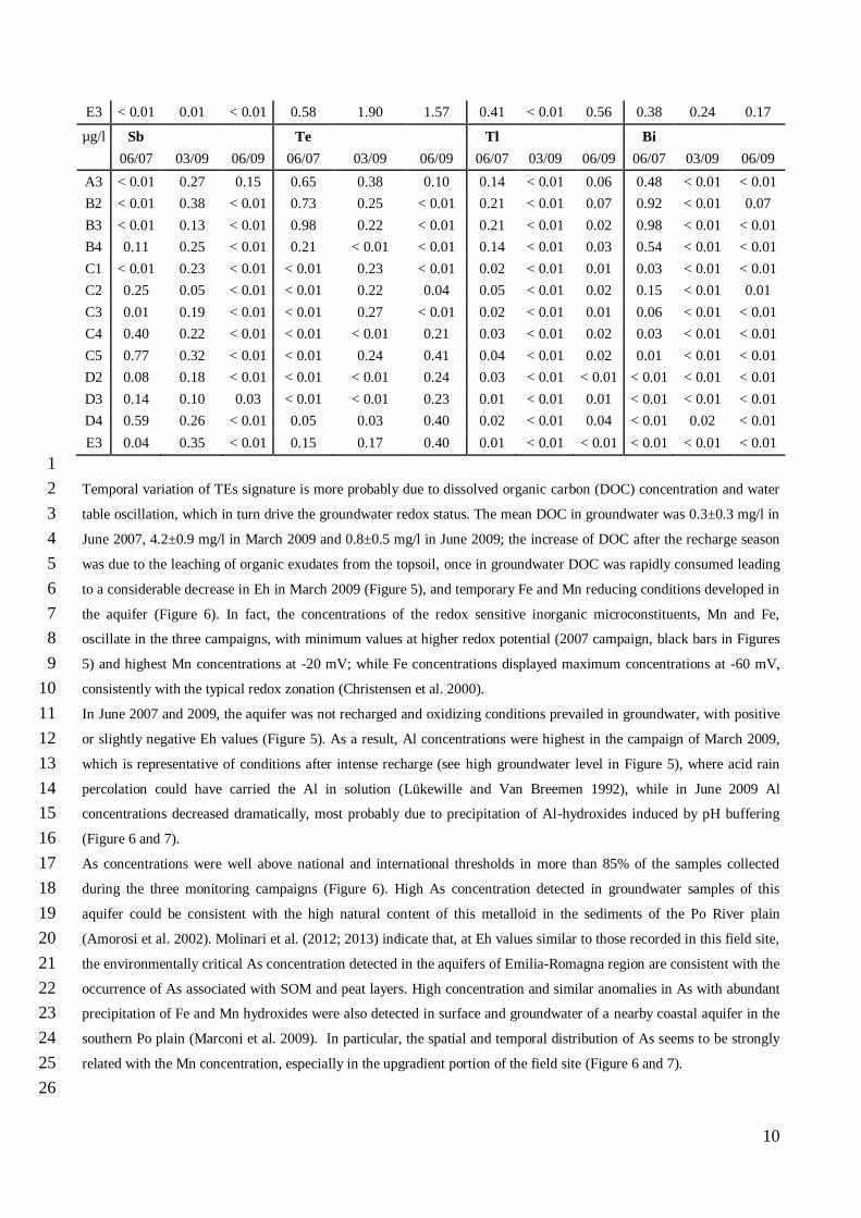
µg/l Sb

Te

Tl

Bi

06/07 03/09 06/09 06/07 03/09 06/09 06/07 03/09 06/09 06/07 03/09 06/09

A3 < 0.01 0.27 0.15 0.65 0.38 0.10 0.14 < 0.01 0.06 0.48 < 0.01 < 0.01

B2 < 0.01 0.38 < 0.01 0.73 0.25 < 0.01 0.21 < 0.01 0.07 0.92 < 0.01 0.07

B3 < 0.01 0.13 < 0.01 0.98 0.22 < 0.01 0.21 < 0.01 0.02 0.98 < 0.01 < 0.01

B4 0.11 0.25 < 0.01 0.21 < 0.01 < 0.01 0.14 < 0.01 0.03 0.54 < 0.01 < 0.01

C1 < 0.01 0.23 < 0.01 < 0.01 0.23 < 0.01 0.02 < 0.01 0.01 0.03 < 0.01 < 0.01

C2 0.25 0.05 < 0.01 < 0.01 0.22 0.04 0.05 < 0.01 0.02 0.15 < 0.01 0.01

C3 0.01 0.19 < 0.01 < 0.01 0.27 < 0.01 0.02 < 0.01 0.01 0.06 < 0.01 < 0.01

C4 0.40 0.22 < 0.01 < 0.01 < 0.01 0.21 0.03 < 0.01 0.02 0.03 < 0.01 < 0.01

C5 0.77 0.32 < 0.01 < 0.01 0.24 0.41 0.04 < 0.01 0.02 0.01 < 0.01 < 0.01

D2 0.08 0.18 < 0.01 < 0.01 < 0.01 0.24 0.03 < 0.01 < 0.01 < 0.01 < 0.01 < 0.01

D3 0.14 0.10 0.03 < 0.01 < 0.01 0.23 0.01 < 0.01 0.01 < 0.01 < 0.01 < 0.01

D4 0.59 0.26 < 0.01 0.05 0.03 0.40 0.02 < 0.01 0.04 < 0.01 0.02 < 0.01

E3 0.04 0.35 < 0.01 0.15 0.17 0.40 0.01 < 0.01 < 0.01 < 0.01 < 0.01 < 0.01

1

Temporal variation of TEs signature is more probably due to dissolved organic carbon (DOC) concentration and water 2

table oscillation, which in turn drive the groundwater redox status. The mean DOC in groundwater was 0.3±0.3 mg/l in 3

June 2007, 4.2±0.9 mg/l in March 2009 and 0.8±0.5 mg/l in June 2009; the increase of DOC after the recharge season 4

was due to the leaching of organic exudates from the topsoil, once in groundwater DOC was rapidly consumed leading 5

to a considerable decrease in Eh in March 2009 (Figure 5), and temporary Fe and Mn reducing conditions developed in 6

the aquifer (Figure 6). In fact, the concentrations of the redox sensitive inorganic microconstituents, Mn and Fe, 7

oscillate in the three campaigns, with minimum values at higher redox potential (2007 campaign, black bars in Figures 8

5) and highest Mn concentrations at -20 mV; while Fe concentrations displayed maximum concentrations at -60 mV, 9

consistently with the typical redox zonation (Christensen et al. 2000). 10

In June 2007 and 2009, the aquifer was not recharged and oxidizing conditions prevailed in groundwater, with positive 11

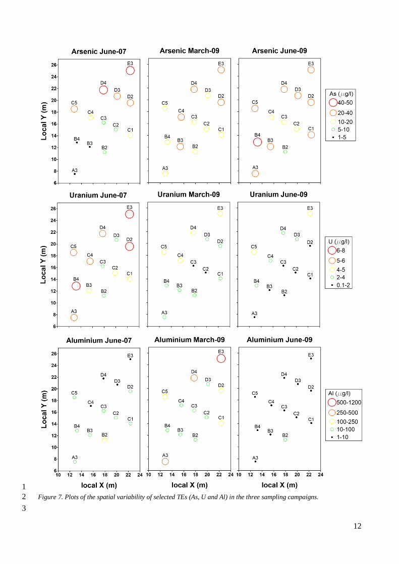
or slightly negative Eh values (Figure 5). As a result, Al concentrations were highest in the campaign of March 2009, 12

which is representative of conditions after intense recharge (see high groundwater level in Figure 5), where acid rain 13

percolation could have carried the Al in solution (Lükewille and Van Breemen 1992), while in June 2009 Al 14

concentrations decreased dramatically, most probably due to precipitation of Al-hydroxides induced by pH buffering 15

(Figure 6 and 7). 16

As concentrations were well above national and international thresholds in more than 85% of the samples collected 17

during the three monitoring campaigns (Figure 6). High As concentration detected in groundwater samples of this 18

aquifer could be consistent with the high natural content of this metalloid in the sediments of the Po River plain 19

(Amorosi et al. 2002). Molinari et al. (2012; 2013) indicate that, at Eh values similar to those recorded in this field site, 20

the environmentally critical As concentration detected in the aquifers of Emilia-Romagna region are consistent with the 21

occurrence of As associated with SOM and peat layers. High concentration and similar anomalies in As with abundant 22

precipitation of Fe and Mn hydroxides were also detected in surface and groundwater of a nearby coastal aquifer in the 23

southern Po plain (Marconi et al. 2009). In particular, the spatial and temporal distribution of As seems to be strongly 24

related with the Mn concentration, especially in the upgradient portion of the field site (Figure 6 and 7). 25

26

11

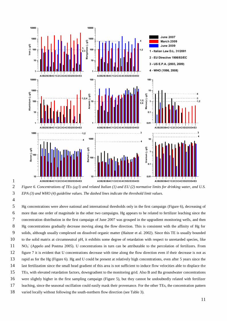
1

Figure 6. Concentrations of TEs (μg/l) and related Italian (1) and EU (2) normative limits for drinking water, and U.S. 2

EPA (3) and WHO (4) guideline values. The dashed lines indicate the threshold limit values. 3

4

Hg concentrations were above national and international thresholds only in the first campaign (Figure 6), decreasing of 5

more than one order of magnitude in the other two campaigns. Hg appears to be related to fertilizer leaching since the 6

concentration distribution in the first campaign of June 2007 was grouped in the upgradient monitoring wells, and then 7

Hg concentrations gradually decrease moving along the flow direction. This is consistent with the affinity of Hg for 8

solids, although usually complexed on dissolved organic matter (Haitzer et al. 2002). Since this TE is usually bounded 9

to the solid matrix at circumneutral pH, it exhibits some degree of retardation with respect to unretarded species, like 10

NO3- (Appelo and Postma 2005). U concentrations in turn can be attributable to the percolation of fertilizers. From 11

figure 7 it is evident that U concentrations decrease with time along the flow direction even if their decrease is not as 12

rapid as for the Hg (Figure 6). Hg and U could be present at relatively high concentrations, even after 5 years since the 13

last fertilization since the small head gradient of this area is not sufficient to induce flow velocities able to displace the 14

TEs, with elevated retardation factors, downgradient to the monitoring grid. Also B and Ba groundwater concentrations 15

were slightly higher in the first sampling campaign (Figure 5), but they cannot be undoubtedly related with fertilizer 16

leaching, since the seasonal oscillation could easily mask their provenance. For the other TEs, the concentration pattern 17

varied locally without following the south-northern flow direction (see Table 3). 18

12

1

Figure 7. Plots of the spatial variability of selected TEs (As, U and Al) in the three sampling campaigns. 2

3

13

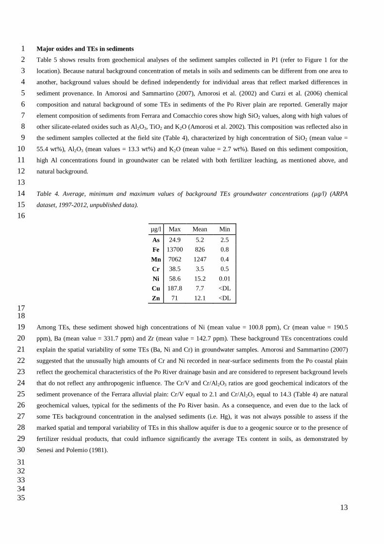
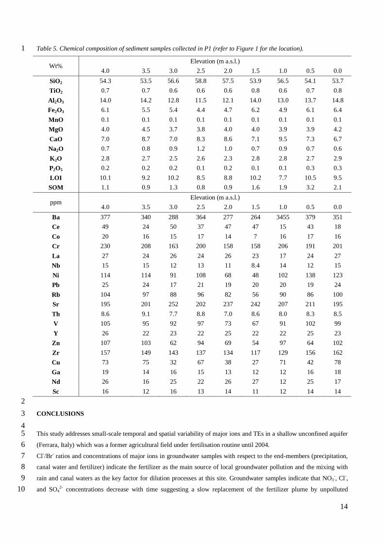
Major oxides and TEs in sediments 1

Table 5 shows results from geochemical analyses of the sediment samples collected in P1 (refer to Figure 1 for the 2

location). Because natural background concentration of metals in soils and sediments can be different from one area to 3

another, background values should be defined independently for individual areas that reflect marked differences in 4

sediment provenance. In Amorosi and Sammartino (2007), Amorosi et al. (2002) and Curzi et al. (2006) chemical 5

composition and natural background of some TEs in sediments of the Po River plain are reported. Generally major 6

element composition of sediments from Ferrara and Comacchio cores show high SiO2 values, along with high values of 7

other silicate-related oxides such as Al2O3, TiO2 and K2O (Amorosi et al. 2002). This composition was reflected also in 8

the sediment samples collected at the field site (Table 4), characterized by high concentration of SiO2 (mean value = 9

55.4 wt%), Al2O3 (mean values = 13.3 wt%) and K2O (mean value = 2.7 wt%). Based on this sediment composition, 10

high Al concentrations found in groundwater can be related with both fertilizer leaching, as mentioned above, and 11

natural background. 12

13

Table 4. Average, minimum and maximum values of background TEs groundwater concentrations (µg/l) (ARPA 14

dataset, 1997-2012, unpublished data). 15

16

µg/l Max Mean Min

As 24.9 5.2 2.5

Fe 13700 826 0.8

Mn 7062 1247 0.4

Cr 38.5 3.5 0.5

Ni 58.6 15.2 0.01

Cu 187.8 7.7 <DL

Zn 71 12.1 <DL

17 18

Among TEs, these sediment showed high concentrations of Ni (mean value = 100.8 ppm), Cr (mean value = 190.5 19

ppm), Ba (mean value = 331.7 ppm) and Zr (mean value = 142.7 ppm). These background TEs concentrations could 20

explain the spatial variability of some TEs (Ba, Ni and Cr) in groundwater samples. Amorosi and Sammartino (2007) 21

suggested that the unusually high amounts of Cr and Ni recorded in near-surface sediments from the Po coastal plain 22

reflect the geochemical characteristics of the Po River drainage basin and are considered to represent background levels 23

that do not reflect any anthropogenic influence. The Cr/V and Cr/Al2O3 ratios are good geochemical indicators of the 24

sediment provenance of the Ferrara alluvial plain: Cr/V equal to 2.1 and Cr/Al2O3 equal to 14.3 (Table 4) are natural 25

geochemical values, typical for the sediments of the Po River basin. As a consequence, and even due to the lack of 26

some TEs background concentration in the analysed sediments (i.e. Hg), it was not always possible to assess if the 27

marked spatial and temporal variability of TEs in this shallow aquifer is due to a geogenic source or to the presence of 28

fertilizer residual products, that could influence significantly the average TEs content in soils, as demonstrated by 29

Senesi and Polemio (1981). 30

31

32

33

34

35

14

Table 5. Chemical composition of sediment samples collected in P1 (refer to Figure 1 for the location). 1

Wt% Elevation (m a.s.l.)

4.0 3.5 3.0 2.5 2.0 1.5 1.0 0.5 0.0

SiO2 54.3 53.5 56.6 58.8 57.5 53.9 56.5 54.1 53.7

TiO2 0.7 0.7 0.6 0.6 0.6 0.8 0.6 0.7 0.8

Al2O3 14.0 14.2 12.8 11.5 12.1 14.0 13.0 13.7 14.8

Fe2O3 6.1 5.5 5.4 4.4 4.7 6.2 4.9 6.1 6.4

MnO 0.1 0.1 0.1 0.1 0.1 0.1 0.1 0.1 0.1

MgO 4.0 4.5 3.7 3.8 4.0 4.0 3.9 3.9 4.2

CaO 7.0 8.7 7.0 8.3 8.6 7.1 9.5 7.3 6.7

Na2O 0.7 0.8 0.9 1.2 1.0 0.7 0.9 0.7 0.6

K2O 2.8 2.7 2.5 2.6 2.3 2.8 2.8 2.7 2.9

P2O5 0.2 0.2 0.2 0.1 0.2 0.1 0.1 0.3 0.3

LOI 10.1 9.2 10.2 8.5 8.8 10.2 7.7 10.5 9.5

SOM 1.1 0.9 1.3 0.8 0.9 1.6 1.9 3.2 2.1

ppm Elevation (m a.s.l.)

4.0 3.5 3.0 2.5 2.0 1.5 1.0 0.5 0.0

Ba 377 340 288 364 277 264 3455 379 351

Ce 49 24 50 37 47 47 15 43 18

Co 20 16 15 17 14 7 16 17 16

Cr 230 208 163 200 158 158 206 191 201

La 27 24 26 24 26 23 17 24 27

Nb 15 15 12 13 11 8.4 14 12 15

Ni 114 114 91 108 68 48 102 138 123

Pb 25 24 17 21 19 20 20 19 24

Rb 104 97 88 96 82 56 90 86 100

Sr 195 201 252 202 237 242 207 211 195

Th 8.6 9.1 7.7 8.8 7.0 8.6 8.0 8.3 8.5

V 105 95 92 97 73 67 91 102 99

Y 26 22 23 22 25 22 22 25 23

Zn 107 103 62 94 69 54 97 64 102

Zr 157 149 143 137 134 117 129 156 162

Cu 73 75 32 67 38 27 71 42 78

Ga 19 14 16 15 13 12 12 16 18

Nd 26 16 25 22 26 27 12 25 17

Sc 16 12 16 13 14 11 12 14 14

2

CONCLUSIONS 3

4 This study addresses small-scale temporal and spatial variability of major ions and TEs in a shallow unconfined aquifer 5

(Ferrara, Italy) which was a former agricultural field under fertilisation routine until 2004. 6

Cl-/Br- ratios and concentrations of major ions in groundwater samples with respect to the end-members (precipitation, 7

canal water and fertilizer) indicate the fertilizer as the main source of local groundwater pollution and the mixing with 8

rain and canal waters as the key factor for dilution processes at this site. Groundwater samples indicate that NO3-, Cl-, 9

and SO42- concentrations decrease with time suggesting a slow replacement of the fertilizer plume by unpolluted 10

15

groundwater. However, elevated TEs concentrations are still recorded in groundwater, after 5 years since the last 1

fertilisation. High TEs values could be due both to past agricultural practices and to natural background TEs content. 2

Data indicate that the dominant process involved in determining small scale spatial variability of TEs content in this 3

shallow aquifer is the sediment-water interaction. The temporal variation of TEs signature is due to the organic matter 4

content and water table oscillation, which in turn drive the groundwater redox status and the mobilization of some 5

inorganic microconstituents, such as Fe and Mn. Even at small scale and in a relative homogeneous aquifer, spatial and 6

temporal variations in major ions and TEs contents can be found throughout the aquifer. This study emphasizes the need 7

of small scale temporal and spatial resolution to infer anthropogenic TEs contamination, in order to discriminate 8

between non-point sources of pollution (like fertilizers) and background concentrations. Finally, this study underlines 9

the need of having a dense monitoring well network and several monitoring campaigns to ensure that the temporal and 10

spatial variability could be accurately represented. 11

12

REFERENCES 13

14

Abdel-Haleem, A.S., Sroor, A., El-Bahi, S.M., & Zohny, E. (2001). Heavy metals and rare earth elements in phosphate 15

fertilizer components using instrumental neutron activation analysis. Applied Radiation and Isotopes, 55, 569-573. 16

Amorosi, A., Centineo, M.C., Dinelli, E., Lucchini, F., & Tateo, F. (2002). Geochemical and mineralogical variations as 17

indicators of provenance changes in Late Quaternary deposits of SE Po Plain. Sedimentary Geology, 151, 273-292. 18

Amorosi, A., Colalongo, M.L., Fusco, F., Pasini, G., & Fiorini, F. (1999). Glacio-eustatic control of continental-shallow 19

marine cyclicity from Late Quaternary deposits of the south-eastern Po Plain (Northern Italy). Quaternary 20

Resources, 52, 1-13. 21

Amorosi, A., & Sammartino, I. (2007). Influence of sediment provenance on background values of potential toxic 22

metals from near-surface sediments of Po coastal plain (Italy). International Journal of Earth Sciences, 96, 389-396. 23

Appelo, C.A.J., & Postma, D. (2005). Geochemistry, Groundwater and Pollution 2nd Edition. Balkema, Rotterdam. 24

Christensen, T.H., Bjerg, P.L., Banwart, S.A., Jakobsen, R., Heron, G., & Albrechtsen, H. (2000). Characterization of 25

redox conditions in groundwater contaminant plumes. Journal of Contaminant Hydrology, 45, 165-241. 26

Curzi, P.V., Dinelli, E., Ricci Lucchi, M., & Vaiani, S.C. (2006). Palaeoenvironmental control on sediment composition 27

and provenance in the late Quaternary deltaic succession: a case study from the Po delta area (Northern Italy). 28

Geological Journal, 41, 591-612. 29

Davis, S.N., Whittemone, D.O., & Fabryka-Martin, J. (1998). Uses of chloride/bromide ratios in studies of potable 30

water. Ground Water, 36 (2), 338–350. 31

D.L. 31/2001. Decreto legislativo 2 febbraio 2001, n. 31, attuazione della direttiva 98/83/CE relativa alla qualità delle 32

acque destinate al consumo umano. Gazzetta Ufficiale n. 52 del 03/03/2001. 33

EU Directive 98/83/CE. (1998). Council Directive of 3 November 1998 on the quality of water intended for human 34

consumption. Official Journal of the European Union L 330; 32 (5/12/1998). 35

Galloway, J.N., Townsend, A.R., Erisman, J.W., Bekunda, M., Cai, Z., Freney, J.R., Martinelli, L.A., et al. (2008). 36

Transformation of the nitrogen cycle: recent trends, questions, and potential solutions. Science, 320, 889-892. 37

Gehl, R.J., Schmidt, J.P., Stone, L.R., Schlegel, A.J., & Clark, G.A. (2002). In situ measurements of nitrate leaching 38

implicate poor nitrogen and irrigation management on sandy soil. Journal of Environmental Quality, 34, 2243-2254. 39

Haitzer, M., Aiken, G.R., & Ryan, J.N. (2002). Binding or mercury (II) to dissolved organic matter: the role of the 40

mercury-to-DOM concentration ratio. Environmental Science and Technology, 36, 3564-70. 41

16

Helena, B., Pardo, R., Vega, M., Barrado, E., Fernandez, J.M., & Fernandez, L. (2000). Temporal evolution of 1

groundwater composition in an alluvial aquifer (Pisuerga River, Spain) by principal component analysis. Water 2

Researches, 34(3), 807-816. 3

Ibendahl, G., & Fleming, R., A. (2007). Controlling aquifer nitrogen levels when fertilizing crops: a study of 4

groundwater contamination and denitrification. Ecological Modelling, 205, 507-514. 5

Katz, B.K., Ebert, S.M., & Kauffman, L.J. (2011). Using Cl/Br ratios and other indicators to assess potential impacts on 6

groundwater quality from septic systems: A review and examples from principal aquifers in the United States. 7

Journal of Hydrology, 397, 151-166. 8

Köhler, K., Duynisveld, W.H.M., & Böttcher, J. (2006). Nitrogen fertilization and nitrate leaching into groundwater on 9

arable sandy soils. Journal of Plant Nutrition and Soil Science, 169, 185-195. 10

Lükewille, A., & Van Breemen, N. (1992). Aluminium precipitates from groundwater of an aquifer affected by acid 11

atmospheric deposition in the Senne, northern Germany. Water, Air, and Soil Pollution, 63, 411-416. 12

Marconi, V., Dinelli, E., Antonellini, M., Capaccioni, B., Balugani, E., & Gabbianelli, G. (2009). Hydrogeochemical 13

characterization of the phreatic system of the coastal wetland located between Fiumi Uniti and Bevano rivers in the 14

southern Po plain (Northern Italy). Geophysical Research Abstract 11, EGU2009-9771, EGU General Assembly 15

2009. 16

Mastrocicco, M., Vignoli, G., Colombani, N., & Abu Zeid, N. (2010). Surface electrical resistivity tomography and 17

hydrogeological characterization to constrain groundwater flow modelling in an agricultural field site near Ferrara 18

(Italy). Environmental Earth Sciences, 61(2), 311-322. 19

Mastrocicco, M., Colombani, N., Castaldelli, G., & Jovanovic, N. (2011). Monitoring and modelling nitrate persistence 20

in a shallow aquifer. Water, Air, & Soil Pollution, 217(1-4), 83-93. 21

Mastrocicco, M., Giambastiani, B.M.S., Severi, P., & Colombani, N., (2012). The importance of data acquisition 22

techniques in saltwater intrusion monitoring. Water Resources Management, 26, 2851-2866. 23

McMahon, P.B., Böhlke, J.K., Kauffman, L.J., Kipp, K.L., Landon, M.K., Crandall, C.A., et al. (2008). Source and 24

transport controls on the movement of nitrate to public supply wells in selected principal aquifers of the United 25

States. Water Resources Research, 44, 1-17. 26

Molinari, A., Guadagnini, L., Marcaccio, M., & Guadagnini, A. (2012). Natural background levels and threshold values 27

of chemical species in three large-scale groundwater bodies in Northern Italy. Science of the Total Environment, 28

425, 9-19. 29

Molinari, A., Guadagnini, L., Marcaccio, M., Straface, S., Sanchez-Villa, X., & Guadagnini, A. (2013). Arsenic release 30

from deep natural solid matrices under experimentally controlled redox conditions. Science of the Total 31

Environment, 44, 231-240. 32

Nouri, J., Mahvi, A.H., Jahed, G.R, & Babaei, A.A. (2008). Regional distribution pattern of groundwater heavy metals 33

resulting from agricultural activities. Environmental Geology, 55, 1337-1343. 34

Otero, N., Vitòria, L., Soler, A., & Canals, A. (2005). Fertilizer characterisation: Major, trace and rare earth elements. 35

Applied Geochemistry, 20, 1473-1488. 36

Perego, A., Basile, A., Bonfante, A., De Mascellis, R., Terribile, F., Brenna, S., & Acutis, M. (2012). Nitrate leaching 37

under maize cropping systems in Po Valley (Italy). Agriculture, Ecosystems and Environment, 147, 57-65. 38

Senesi, N., & Polemio, M. (1981). Trace element addition to soil by application of NPK fertilizers. Fertilizer Research, 39

2, 289-302. 40

17

Stark, C.H., & Richards, K.G. (2008). The continuing challenge of agricultural nitrogen loss to the environment in the 1

context of global change and advancing research. Dynamic Soil Dynamic Plant, 2, 1-12. 2

Tiessen, H., & Moir, J.O. (1993) Total and organic carbon. In M.R. Carter (Ed.), Soil sampling and methods of analysis, 3

Chapter 21 (pp. 187–211). Lewis Publishers. 4

U.S.EPA. (2009). http://water.epa.gov/drink/contaminants/index.cfm#inorganic. Accessed 9 Jul 2014. 5

U.S.EPA. (2003). Drinking water standards. Office of Drinking Water. US Environmental Protection Agency, 6

Washington, DC. 7

Vengosh, A., & Pankratov, I. (1998). Chloride/bromide and chloride/fluoride ratios of domestic sewage effluents and 8

associated contaminated ground water. Ground Water, 36, 815-824. 9

WHO (1996). Guidelines for drinking-water quality, 2nd ed. Health criteria and other supporting information, vol. 2. 10

World Health Organization, Geneva. 11

WHO (2008). Guidelines for drinking-water quality, 3rd ed. Recommendations. Incorporating 1st and 2nd Addenda, vol. 12

1. World Health Organization, Geneva. 13

Wongsasuluk, P., Chotpantarat, S., Siriwong, W., & Robson, M. (2014). Heavy metal contamination and human health 14

risk assessment in drinking water from shallow groundwater wells in an agricultural area in Ubon Ratchathani 15

province, Thailand. Environmental Geochemistry and Health, 36(1), 169-182. 16

Zhao, K., Liu, X., Xu, J., & Selim, H.M. (2010). Heavy metal contaminations in a soil–rice system: Identification of 17

spatial dependence in relation to soil properties of paddy fields. Journal of Hazardous Materials, 181, 778-787. 18

24