Using Environmental Tracers in Modeling Flow in a Complex Shallow Aquifer System

Using Environmental Tracers in Modeling Flow in a ComplexShallow Aquifer System

L. Troldborg1; K. H. Jensen2; P. Engesgaard3; J. C. Refsgaard4; and K. Hinsby5

Abstract: Using environmental tracers in groundwater dating partly relies on the assumption that groundwater age distribution can bedescribed analytically. To investigate the applicability of age dating in complex multiaquifer systems, a methodology for simulating wellspecific groundwater age distribution was developed. Using a groundwater model and particle tracking we modeled age distributions atscreen locations. By enveloping modeled age distributions and estimated recharge concentrations, environmental tracer breakthroughswere simulated for specific screens. Simulated age distributions are of irregular shapes and sizes without being similar to the assumed agedistributions used in the analytical approach. The shape of age distribution to some extent depends on sampling size and on whether thesystem is modeled in a transient or in a steady state, but shape and size were largely driven by the heterogeneity of the model and bytopographical variations as well. Analytically derived groundwater ages are dependent on sampling time. This time dependence relates tothe nonlinearity of recharge concentrations and the shape and size of age distribution that has no coherence with the simplified assump-tions of traditional approaches. Accordingly, constraining flow models by “age observations” may lead to misrepresentations that arebiased depending on sampling time. If environmental tracers are used directly in terms of concentrations instead of ages, spatial as wellas temporal variations become useful in constraining models.

DOI: 10.1061/�ASCE�1084-0699�2008�13:11�1037�

CE Database subject headings: Groundwater management; Hydrogeology; Aquifers; Groundwater flow.

Introduction

Modeling of groundwater flow and transport requires quantifica-tion of hydraulic parameters that may exhibit a large variation inspace and boundary conditions that may vary in both space andtime. Model parameterization is accomplished by using all avail-able geological, hydrogeological, and hydrological data. In thisrespect, a complicating factor and partially unknown geologicaland hydrogeological heterogeneity, which is impossible to quan-tify in all details, are always present. Hence, by necessity, theparameterization needs to be based partially on calibration, e.g.,using inverse modeling techniques. Consequently, model simula-tions will be subject to uncertainty. Tracers have been used tofurther constrain groundwater models and estimate hydraulic pa-rameters. By injecting tracers in the groundwater system whilemonitoring their migration, the spreading of useful information

1Professor, Geological Survey of Denmark and Greenland, ØsterVoldgade 10, DK-1350 Copenhagen K, Denmark �corresponding author�.E-mail: [email protected]

2Professor, Dept. of Geography and Geology, Univ. of Copenhagen,Øster Voldgade 10, DK-1350 Copenhagen K., Denmark. E-mail:[email protected]

3Dept. of Geography and Geology, Univ. of Copenhagen, ØsterVoldgade 10, DK-1350 Copenhagen K, Denmark. E-mail: [email protected]

4Professor, Geological Survey of Denmark and Greenland, ØsterVoldgade 10, DK-1350 Copenhagen K, Denmark. E-mail: [email protected]

5Geological Survey of Denmark and Greenland, Øster Voldgade 10,DK-1350 Copenhagen K, Denmark. E-mail: [email protected]

Note. Discussion open until April 1, 2009. Separate discussions mustbe submitted for individual papers. The manuscript for this paper wassubmitted for review and possible publication on February 2, 2007; ap-proved on June 4, 2008. This paper is part of the Journal of HydrologicEngineering, Vol. 13, No. 11, November 1, 2008. ©ASCE, ISSN 1084-
0699/2008/11-1037–1048/$25.00.
JOURNAL O

Downloaded 08 Dec 2008 to 195.41.77.253. Redistribution subject to

can be obtained on the hydraulic characteristics of the system.However, tracer experiments using artificial tracers are laboriousand costly and are only feasible at dedicated locations and are notuseful for regional systems. Instead, environmental tracers havebeen used to obtain information on flow pathways, travel times,groundwater age, and recharge rates.

Environmental tracers for dating of young groundwater can bedivided in two major groups: �1� event markers, which are re-leased during events that occur over a relatively short time inter-val, such as tritium; and �2� tracers, that are continuously releasedover a long period of time, e.g., chlorofluorocarbons �CFCs��Plummer and Busenberg 2000�. Environmental tracers have theadvantage over artificial tracers to have been present in hydrologi-cal systems for a long time and to have been distributed globally.A complicating factor is that input functions can only be definedto a certain approximation, which complicates the interpretationof tracer data. Nevertheless, environmental tracers may providevaluable information potentially useful for parameterization ofgroundwater models.

Environmental tracers such as tritium/helium-3 3He / 3H,carbon-14 �14C�, CFCs, sulfur hexafluoride �SF6�, and krypton-85�85Kr� have been widely used for age dating of groundwater�Busenberg and Plummer 2000; Cook and Herczeg 2000; Cookand Solomon 1997; Ekwurzel et al. 1994; Cook et al. 1995;Dunkle et al. 1993; Plummer and Busenberg 2000; Solomon et al.1992, 1993; Szabo et al. 1996; Varni and Carrera 1998�. Ground-water age is defined as the time elapsed since the recharge waterentered the groundwater zone and became isolated from the at-mosphere. Most common age computation has been carried outby assuming that a water parcel, when isolated from the atmo-sphere at the water table, is transported by advection along astreamline as piston flow without being subject to dispersion and
diffusion. Varni and Carrera �1998� refer to the age computed
F HYDROLOGIC ENGINEERING © ASCE / NOVEMBER 2008 / 1037

ASCE license or copyright; see http://pubs.asce.org/copyright

hereby as the kinematic age or the radiometric age if the tracerundergoes radioactive decay. Less commonly more refined ana-lytical transfer functions have been applied based on a priori as-sumptions of the age distributions �Zoellmann et al. 2001�. Thesimple transfer models for groundwater dating have proven usefuland robust when applied to homogeneous shallow aquifers andreliable estimates of the age distributions have been obtainedunder such conditions particularly when multiple tracers are usedand when combined with flow and transport modeling �Reillyet al. 1994; Szabo et al. 1996; Portniaguine and Solomon 1998�.

Information on groundwater age can be useful for identifyingthe parts of an aquifer, which could become affected by anthro-pogenic activities �Hinsby et al. 2001�. The age data can also beused to constrain the parameters of groundwater flow and trans-port models and evaluate the history and fate of contaminants�Bohlke and Denver 1995�. Portniaguine and Solomon �1998�used inversion to parameterize an unconfined aquifer at CapeCod, Mass.; Reilly et al. �1994� used age data to calibrate agroundwater flow and path line model for a site in Maryland; andSzabo et al. �1996� reported a similar analysis for a coastal plainaquifer. In these studies, simulations of groundwater ages, havingthe advantage of being tracer independent, were carried out, andsimulation results can be compared directly to ages determinedfrom dating techniques. Misinterpretations, however, will occurif transport mechanisms in the aquifer are different from thoseassumed in the transfer or in the numerical model used to deriveage dates.

Several papers have emphasized that estimates of agedates may be in error if dispersion is significant due to eitheraquifer heterogeneity or mixing in the screens of sampling wells�Goode 1996; Varni and Carrera 1998; Bethke and Johnson 2002;Weismann et al. 2002�. Mixing ratios between waters of differentages can be evaluated solely by evaluating the contents ofmultiple tracers. However, this is mainly an option for binarymixtures where one of the water types is without modern tracerslike 3H, 85Kr, and CFCs �Loosli et al. 2000; Plummer and Busen-berg 2000�. Varni and Carrera �1998� examined the validity of thekinematic age concept for moderately heterogeneous aquifers andcame to the conclusion that the kinematic age is ill posed whenthe systems are heterogeneous or dilution processes take place.They regarded this as a motivation for developing steady-stateand transient equations for the mean age and higher-order mo-ments. Their simulations of mean age exhibit a smooth and morerealistic spatial pattern and, furthermore, they demonstrated thatage estimates may deviate from the mean age of a water samplewhen mixing processes occur, as has also been demonstrated bythe use of multiple tracers �Loosli et al. 2000�. Weissmann et al.�2002� analyzed groundwater ages in the Kings River alluvialfan aquifer system in California where hydrofacies distributionwas generated using a transition probability geostatistical ap-proach. Flow and transport were simulated for this system usingMODFLOW and a backward particle tracking method for rela-tively simple imposed flow boundary conditions. Numericalsimulations of groundwater ages were carried out and simulatedactual mean ages were compared to simulated CFC ages. Also,their results clearly illustrated that the representation of ground-water age by a single value/date can be misleading.

In this study we examine age distribution in a shallow com-plex aquifer system located in the central part of Denmark. Theaquifer system is dominated by large-scale heterogeneity andcomplex flow boundary conditions. We apply a forward particletracking method for the simulation of age distribution. The con-
volution integral approach is used for computing concentrations
1038 / JOURNAL OF HYDROLOGIC ENGINEERING © ASCE / NOVEMBER


of multiple environmental tracers based on a single particle track-ing simulation and respective input functions for the various trac-ers. The simulated tracer concentrations are compared tomeasured concentrations, and simulated ages are compared to themean ages derived from tracer data using standard techniques.

Site and Data Description

The aquifer investigated system is located in the central part ofFunen, just south of Odense, Denmark �Fig. 1�. This system hasbeen used for water supply purposes for more than 100 years.Due to increasing water quality problems in production wells inrecent years, much attention has been given to groundwater flowand the respective distribution of residence time in the aquifersystem �e.g., Hinsby et al. 2004�.

The flow characteristics of the aquifer system and aquifer/stream interaction are significantly affected by results of glacialactivity during the main Weichselian �north-east� and young Bal-tic �south-east� advances. During the young Baltic advances, thecentral parts of Funen were covered by dead ice masses from theformer advances, preserving the NE-SW alignment of topographyin the upper parts of the catchment. During recession, meltwaterstreams flowing through central parts of Funen deposited largeamounts of sand, gravel and clay, forming the floodplain valleys�Houmark-Nielsen 1987; Larsen 2002; Mertz 1974; Windolf2002�. The glacial overburden constitutes 30–80 m of a complexsequence of clayey and sandy tills, glaciofluvial sand, and graveldeposits. The main aquifers are found in semiconfined units ofglaciofluvial sand, gravel deposits at varying depths overlain byglacial till. Tertiary marls and clay form the lower boundary of theQuaternary aquifer system. The aquifer system is drained by theOdense stream flowing in a northeasterly direction towards thesea.

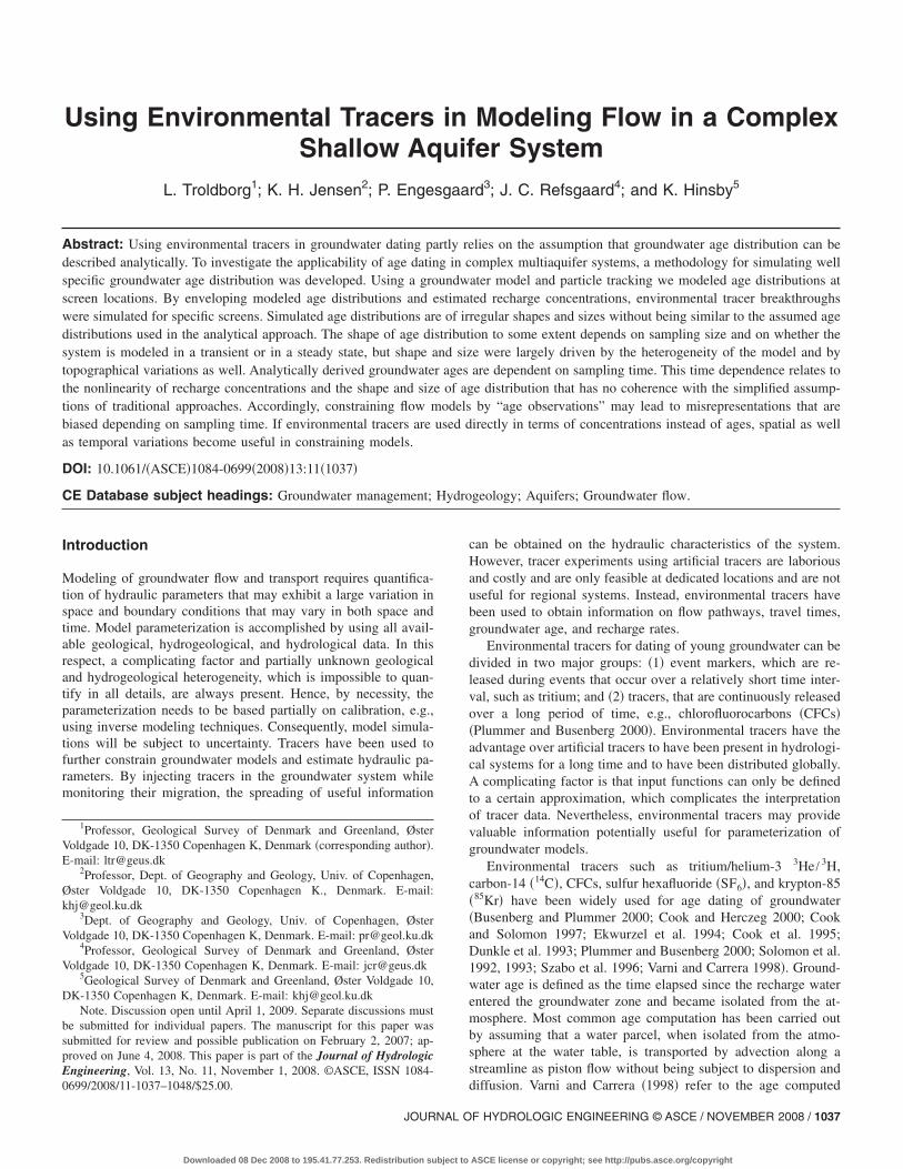
Despite the complexity and heterogeneity of the aquifer sys-tem, it is possible to identify two fairly homogeneous and con-tinuous glaciofluvial sand/gravel units throughout the study area,serving as main aquifers of the area. The geological cross sectionshown in Fig. 2 provides a representation of geological complex-ity. In most of the catchment area, the sand/gravel units are inter-preted to be separated by glacial till of varying sand content,whereas separation between the units near the Odense stream ismissing in some areas. The extensive well log archive on litho-logical information shows that the typical thickness of the twoglaciofluvial units is 10–15 m. In the northwestern parts of thecatchment, a third unit of sand and gravel is present within theglacial till, but it is believed to be discontinuous and isolatedwithout direct contact to the two other units. The majority of morethan 1,000 well logs from the study area provides information onthe upper 30 m while only 10% of wells penetrate the wholeQuaternary sequence down to the Tertiary clay. Consequently,defining the hydrogeological complexity is subject to uncertainty.This uncertainty is further aggravated by the tendency of wells tocluster in near-stream areas as well as in central parts of Odensecity.

The catchment is characterized by an undulating surface cutby numerous tributaries and a relatively large topographical varia-tion ranging from 2 to 120 m above sea level �a.s.l.� within aradius of 10 km. Most of the area is artificially drained due toagricultural interests and the general high-precipitation climate.The tributaries are small and well connected to the drainage sys-tem, and they respond quickly to rain events. Based on climatic
records from 1991 to 2000, annual precipitation ranges from 580
2008


to 1,030 mm /year, and annual potential evapotranspiration from480 to 570 mm /year. There is a slight seasonality in precipitationwhile potential evaporation displays a pronounced seasonal varia-tion. Mean annual net precipitation is 390 mm and most of it��90% � occurs in the cold season �October–March�.

Environmental Tracer Data

Measurements of environmental tracer concentrations are avail-able from three wells in the study area, located only a few kmapart �Hinsby et al. 2004�. Well_dvv is a cluster of productionwells with screens in hydrogeological Units 3 and 5, the two mainaquifer units within the catchment area. Well_34 and Well_74 areold production wells, abandoned due to pesticide contaminationindicating that at least part of the water at these wells is less than50 years. Well_34 is screened in hydrogeological Unit 3 and wasclosed in 1989; and Well_74 is screened in hydrogeological Unit5 and was closed in 2001.

Water samples were collected from the three wells in the pe-

Fig. 1. Odense stream catchment area �model area� with locations of

riod 1999–2002 and each sample was analyzed for tracer con-

JOURNAL O


centrations. Samples from Well_34 and Well_74 were sampledand analyzed for 3H, 3He, SF6, 85Kr, and CFC-12 by Climate andEnvironmental Physics, Physics Institute, University of Bern,and the Swiss Federal Institute for Environmental Science andTechnology, EAWAG �Alvarado et al. 2005�. In addition, selectedhistoric water samples were retrieved from water sample archivescollected by the Odense Water Supply Company and covering theperiod 1963–1995 �Hinsby et al. 2006�. These water sampleswere analyzed for 3H by the Isotope Hydrology Laboratory at theInternational Atomic Energy Agency �IAEA, Vienna�. Well_dvvwas sampled and analyzed for CFC-11, CFC-12, CFC-113, SF6,85Kr, 3H, and 3He. Unfortunately, no historic water samples wereavailable for Well_dvv at the water sample archives and, accord-ingly, it was not possible to extend the measurements back in timefor this particular well.

Conceptual Hydrogeological Model

The development of the conceptual hydrogeological model was

elds, topographical variation, and capture zone to investigated wells
well fi
based on a systematic spatial analysis of well core information



with supporting information obtained from the Danish nationalwater resources model �Henriksen et al. 1997� and detailed soilmaps. This analysis resulted in the identification of eight hydro-geological units �Fig. 2� which is summarized in Table 1. The lowpermeable layers are dominated by Quaternary clayey till withoccurrences of smaller amounts of Eocene and Paleocene clay.Hydraulic conductivity is mainly controlled by the heterogeneityof the till, such as the presence of smaller sand pockets and frac-ture density. As this information is not known in detail, hydrogeo-logical Units 2, 4, and 7 are all assumed to have the samehydraulic conductivity and a constant ratio between vertical andhorizontal direction.

The occurrence and extent of fractures in Moraine till and theirimpact on the hydraulic properties and contaminant transporthave been widely documented �Fredericia 1990; McKay et al.

Fig. 2. Cross section �see also Fig. 1� from Odense stream catchm

Table 1. Hydrogeological Model Description

Unit Description K n

1 Partly fractured and permeable till �upper 3 m� KML1 0.2

2 Low permeability layer below upper regionalaquifer �nonfractured till�

KML2 0.2

3 High permeability layer �first regional aquifer,sand, and gravel�

KS 0.2

4 Low permeability layers �till of regional extent� KML2 0.2

5 High permeability layer �second regional aquifer,sand, and gravel�

KS 0.2

6 In the Northern part of the catchment, a highpermeable secondary aquifer of sand and gravelis present within the upper low permeabilitylayer �not shown in Fig. 2�

KS 0.2

7 Lenses of low permeable material that arepresent within the second regional aquifer�Unit 5� parallel to Odense stream, elongated�2,000�100 m2�

KML2 0.2

8 Low permeable Tertiary clay �model bottom� — —



1993; Hinsby et al. 1996; Jørgensen et al. 1998a,b; Klint andGavesen 1999�. No specific hydrogeological field investigationshave been carried out as a part of this study, so it has been as-sumed, based on these earlier Danish studies, which fracturesextend through the upper 3 m of the upper moraine till �Unit 1�.Meltwater sand and gravel are dominant features of Layers 3, 5,and 6, leading to a high permeability. Most production wells arescreened in Units 3 and 5, while Unit 6 is exploited only to alimited extent. As only a few pumping tests are available, it is notpossible to justify any trends in hydraulic conductivity on thisbasis, within the high permeability units. Consequently, it hasbeen assumed that uniform hydraulic parameters within the cali-bration procedure apply to individual units. Tertiary material ofnegligible permeability provides the lower boundary condition ofthe aquifer system.

Processing Environmental Tracers

We constrained simulations to the groundwater zone and its inter-action with streams. The upper boundary condition is in the formof groundwater recharge, and the input functions for the tracersshould, therefore, represent concentration in the recharge water.Records of atmospheric concentrations serve as the basis for es-timating these concentrations. The individual tracers consideredin this study, their specific attributes, and input function charac-teristics are described below.

CFCs are released into the environment from a wide rangeof industrial and refrigerant applications. The input function isderived from atmospheric concentrations, as measured or recon-structed from production records �Busenberg and Plummer 1992/USGS� and recharge temperature, using Henry’s law of solubility.Time lag and dispersion in the unsaturated zone can be dis-regarded for shallow unsaturated zones and relatively high re-charge rates �such as that of the present study area�. CFCs aregenerally considered to behave like a nonreactive tracer but

ith geological information and filter intervals of investigated wells
ent w
some studies have suggested that at least some tracers could be

2008


affected by degradation and adsorption under certain redox con-ditions �Hinsby et al. 2007; Engesgaard et al. 2004; Plummer andBusenberg 2000�.

The source of SF6 is primarily from producers of high voltageswitches �Cook and Herczeg 2000�. Accordingly, atmosphericconcentrations have steadily increased since the 1960s. As forCFC, the input function is calculated from atmospheric concen-trations, which are measured or reconstructed from productionrecords �Busenberg and Plummer 2000/USGS�� and rechargetemperature using Henry’s law of solubility. SF6 concentrations inthe air phase of shallow unsaturated zones �less than 10 m� can beassumed to be in equilibrium with atmospheric concentrations�Busenberg and Plummer 2000�. SF6 acts like an ideal gas and isnot subject to chemical reactions, sorption, or degradation in natu-ral environments �Busenberg and Plummer 2000�. 85Kr is releasedinto the atmosphere from reprocessing of used nuclear fuel rods.Atmospheric 85Kr activity has steadily increased since the mid1950s �Loosli et al. 2000�. 85Kr is chemically inert in ground-water, but undergoes radioactive decay with a half-life of10.76 years �Ekwurzel et al. 1994�. Resembling SF6 and CFCs,85Kr traverses the unsaturated zone primarily by diffusion. Whenthe unsaturated zone is shallow, 85Kr can be assumed in equi-librium with atmospheric concentrations. 85Kr is measuredin 85Kr /Kr ratios �disintegration per minute per cm3 of Kr�dpm /cm3 Kr��. Thus, recharge temperature, degassing, and solu-bility do not influence the construction of the input function. Con-sequently for shallow depths, atmospheric measurements can beapplied directly as input function �Loosli et al. 2000�.

Tritium �3H� was introduced into the stratosphere by atmo-spheric nuclear bomb testing in the late 1950s and early 1960s.Due to seasonal uplift in the troposphere and 3H blending withhigher altitude stratosphere, significant seasonal concentrationvariations are observed in precipitation �Ferronsky and Polyakov1982; Solomon and Cook 2000�. These seasonal variations haveimplications on mass flux to the groundwater zone, as high sum-mer concentrations correspond to low recharge rates and viceversa. Monthly tritium concentrations were synthesized from in-terpolations between monthly measurements at Ottawa and localOdense annual or biannual measurements, both available from theIAEA/WMO database on isotopes in precipitation. Tritium mea-surements are expressed in tritium units ��TU�=one 3H1HO to1018 1H2O� and the solubility is not, like the 85Kr /Kr ratio de-pendent on temperature. Tritium may be treated as a nonreactivetracer, unaffected by both degradation and sorption but subject toradioactive decay to its daughter product, 3He, with a half-life of12.43 years �Solomon and Cook 2000�.

The 3He-input function can be derived from 3H decay. Abovethe water table, 3He is in equilibrium with atmospheric concen-tration �zero concentration� as long as the unsaturated zone isshallow. Below the water table, 3He concentrations are attribut-able to 3He decay �and possible excess air�, as other sources of3He are negligible in most shallow aquifers �Solomon et al.1995�. Gaseous tracers like CFC-11, CFC-12, CFC-113, SF6,85Kr, and 3He are in equilibrium with the air phase of the vadosezone. Depending on solubility, diffusion coefficient, and thicknessof the vadose zone, the air phase will be in equilibrium with theatmosphere. This is especially true if the gas has a low solubilityand a large diffusion coefficient as gas phase diffusion is typicallymuch faster than advective gas transport. The water phase will,accordingly, be in equilibrium with the atmosphere until the waterhas been separated from the soil atmosphere. Obviously, the thin-
ner the unsaturated zone, the more valid this assumption. As the
JOURNAL O


unsaturated zone in the Odense catchment is relatively thin��5 m�, its impact on input functions at the water table is for thesake of simplicity neglected. The constructed input functions forthe above tracers are shown in Fig. 3.

Hydrogeological Modeling

Model Code

The model was constructed using the Mike SHE modeling sys-tem. Mike SHE is a deterministic, fully distributed and integratedhydrological modeling code capable of handling all componentsrelated to the land phase of the hydrological cycle, including sur-face water and groundwater flow �Abbott et al. 1986; Refsgaardand Storm 1995�. In this application, a simplified root-zone modelwas used for preprocessing precipitation and potential evapotrans-piration data into a daily groundwater recharge �net precipitation�time series for specified area distributed vegetation and topsoilcharacteristics �Henriksen et al. 2003�.

Model Setup

The model covers a 15�15 km2 area south of the city ofOdense, �Fig. 1�. A reliable simulation of flow and flow pathlines in a highly complex glacial aquifer system requires athree-dimensional �3D� representation of the important geologicaland hydrogeological structures �Fogg 1986; Frind et al. 2002;Henriksen et al. 2003�. The 3D geological model of the study areawas constructed from the seven hydrogeological units describedabove. Horizontal discretization is 100�100 m, whereas verticaldiscretization varies between 1 and 50 m. The numerical model isbased on six layers identical to hydrogeological Units 1–6. A totalof 78,000 grid cells are included in the groundwater model.

The northern and western boundaries are placed along topo-graphical divides, while the eastern and southern boundaries cutperpendicular to Odense stream �Fig. 1�. As the area and sur-roundings are highly developed with groundwater pumping, a no-flow boundary condition is applied along the model boundary forthe top two layers and for all low-conductivity layers only, whilea head boundary condition is specified for the high-conductivity

Fig. 3. Concentrations of environmental tracers in site-specificrecharging water �input function�

layers at depth. The specified heads appear from simulation re-



sults using a hydrological model for the entire island of Funen�Henriksen et al. 1997�. The exchange between groundwater andstreams �inner boundaries� is defined by a specified leakage pa-rameter and the head difference between stream and adjoininggrid cells. The leakage factor is assumed to be uniform in timeand space. Sixty one pumping wells or well fields are included inthe model. It is estimated that 99% of the total pumping withinthe area is included in the model as only minor wells used foragricultural purposes are not considered. A brief water balanceshows that the bulk of net precipitation flows to the river system,pumping is approximately 10% of the net precipitation, whereasinflow-outflow through boundaries constitutes less than 1%.

The Danish Meteorological Institute provided the time seriesof daily precipitation and potential evapotranspiration data. Landuse and soil maps were obtained from the national data basesystem on geographically localized natural and environmentaldata �Areal Information System �AIS��. Topographical informa-tion was retrieved from the National Survey and Cadastre discreteelement model �DEM� �50 m grid�. The model allows for drain-age runoff based on specified drainage depth �set to 0.5 metersbelow surface �m.b.s.�� and drainage constant �set to 1e-7 L /s�.The alignment of the stream system is adapted from the regionalmodel of the Funen Island �Henriksen et al. 1997�.

Inverse Identification of Hydrogeological ParametersOverparameterization is often seen as one complicating factorwhen using distributed models �Beven 1996�. Thus, adopting arigorous and transparent parameterization procedure, wherebymost parameters are identified directly or indirectly from fielddata in an objective manner and leaving only a small number ofparameters to be identified by calibration, is crucial �Refsgaard1997�. Most parameters related to the surface processes wereadopted directly from the regional hydrological model because oflack of sufficient surface flow observations within the catchmentarea, thus leaving a few selected subsurface hydraulic parametersto be determined by inverse calibration. Assuming steady-stateflow the following parameters were subject to calibration, usingthe inverse code UCODE �Poeter and Hill 1998�:1. Hydraulic conductivity for the upper low permeability unit of

fractured till �KML1� �hydrogeological Unit 1�;2. Hydraulic conductivity for the water bearing units of

outwash sand and gravel �KS� �hydrogeological Units 3, 5,and 6�; and

3. Hydraulic conductivity for low-permeable units of nonfrac-tured clayey till �KML2� �hydrogeological Units 2, 4, and 7�.

This represents a simplification of the area geology which stillcaptures the principal complexity of this multiaquifer system �seeTable 1, Fig. 2�. By assigning uniform hydraulic conductivityvalues to individual hydrogeological units, the groundwater flowand flow path lines will largely be determined by the 3D spatialconfiguration of the geological structure.

The model was autocalibrated by minimizing the aggregatedroot-mean-square value �RMS� of differences between simulatedand measured hydraulic head. Within the model area, 75 headobservations from the upper sand layer �Unit 3�, 16 head obser-vations within the lower sand layer �Unit 5�, and three water levelobservations from the fractured till �Unit 1� were present.

Approach for Modeling Groundwater Ageand Tracers

The groundwater age distributions were simulated using a for-
ward particle tracking procedure in which particle movement was


computed based on simulated local groundwater velocities. Theseflow velocities were obtained from the groundwater component ofMIKE SHE that approximates the 3D groundwater flow equationby an implicit numerical finite difference scheme and solves theset of linear discretized equations using the conjugate gradientmethod �DHI 1999�. Velocities are approximated linearly withineach grid cell based on the midpoint values. The interpolatedvelocity scheme is mass conservative for purely advective particletracking �LaBolle et al. 1996�.

Particles are released with precipitation and are movedthrough the system according to the interpolated velocity field.Mass conservation is achieved as long as particles are releasedproportional to the distributed recharge rate, and particle traveltimes for a given volume are transformed into groundwater agedistribution, assuming steady-state conditions.

Simulation of tracer concentrations and breakthrough curves iscalculated in the following four steps:1. Calculation of age distributions from particle tracking simu-

lation, as described above;2. Construction of an input function at the groundwater table

representing the temporal variation in concentration of theconsidered environmental tracer;

3. Computation of the temporal variation of environmentaltracer concentrations at specific locations �breakthroughcurves� by a convolution integral procedure using the inputfunction for the tracer and the age distribution; and

4. Comparison of simulated and observed tracer concentration.Calculation of the age distribution is the only step that requires

numerical model simulations. The convolution integral step is apostprocessing procedure to be performed for each tracer andeach age distribution.

Groundwater age distributions were computed using a forwardparticle tracking procedure, disregarding local dispersion and dif-fusion. The model includes a 3D description of the large-scalehydrofacies distributions that generate a spreading presumed to behigher than the spreading caused by local dispersion. Weissmannet al. �2002� considered both local dispersion and diffusion intheir analysis, but noted that simulation results were insensitive tochanges in the value of the local dispersivity parameter becauseof associated spreading being secondary to the larger-scalespreading caused by hydrofacies heterogeneity.

The particle tracking simulations continued until reaching anapproximate steady-state condition where the number of particlesexiting through boundaries �wells, streams, and outer boundaries�equals the number released to the system with recharge, in thiscase after �250 years. To assure robust age distributions, how-ever, particle tracking simulation persisted for an additional250 years. The forward particle tracking simulation makes it pos-sible to establish a particle travel time distribution at any givenlocation. This procedure is analogous to simulations in which abackward particle tracking procedure is used to estimate distribu-tions of various travel times from preselected well locations back-ward in time to surface �Tompson et al. 1999; Weissmann et al.2002�. The forward tracking approach implies that particles alsoneed to be tracked outside the area of interest, which increasescomputation time. Additionally, a sufficient number of particlesshould be sampled at a well location to assure a stable age distri-bution estimate, also prolonging computation time.

Travel times are recorded for all particles traversing into aregistration volume around the observation point during the sec-ond 250-simulation period. The frequency of recorded traveltimes is subsequently converted into an age distribution �travel
time histogram�.
2008


Robustness of Age Distribution Simulations

The underlying age distribution is a critical step in deriving thesimulated breakthrough curves of environmental tracers. Theshape of the age distribution is determined by spatial configura-tion of the flow field and its variation in time. In the following,the effects of several hydrogeological features on the break-through curves are examined.

In the analysis described above, the flow field was assumed atsteady state. Subsurface tile drains to facilitate agricultural culti-vation drain most of the area and numerous tributaries intersectthe topography. These factors, in combination with topographicalvariation and complex geology, potentially introduce climatedriven growth and dissipation of local flow systems at shallowdepth. To analyze this issue, a simulation of age distributions wascarried out, considering transients in the flow field.

To prepare results for comparative analysis, steady-state andtransient simulations were based on a hydrological input that re-sulted in the same overall water balance and no yearly change instorage. The steady-state simulations were based on a 10-yearaverage in net precipitation while transient simulations werebased on a daily artificial net precipitation time series generatedby averaging net precipitation for each day within the same10-year period. The transient simulations were carried out withthe artificial time series of daily net precipitation by applying thesame series for each consecutive year until the year-to-year stor-age term approached zero �obtained after 20 years of simulation�.

The impact of transient conditions on flow paths was consid-ered in an expedient manner by extracting 13 flow fields from thetransient flow simulation with a frequency of 28 days. Thesesnapshots are assumed to represent quasi-steady-state conditionsfor the individual periods, constituting the basis for subsequentsimulation of particle tracking. Consequently, only the seasonalvariation was considered �on a near-monthly basis�, whereas theyear-to-year variation was not.

The simulated age distributions based on steady-state condi-tions and the imposed seasonality in flow, are shown in Figs. 4�aand b�, respectively. For Well_34, the two sets of simulations arecomparable; the most important difference being that simulatedage distributions based on transient conditions have a larger frac-tion of particles with a shorter travel time than the distributionsbased on steady-state condition. Well_74, screened in the deeperpart of the aquifer system, shows an opposite trend as a larger

Fig. 4. Simulated groundwater age distributions: �A� age distributiontion; �C� age distribution using steady-state flow and distributed poregistration point as substitute for registration radius

fraction of particles have a longer travel time for transient condi-

JOURNAL O


tions. For Well_dvv, which represents both the upper and lowerparts of the aquifer, the two age distributions are comparable.

Transient flow conditions imply that the shallow part of a mul-tiaquifer becomes younger while the deep part becomes older.The local flow system results in temporal variations in dischargeto boundaries. In this case, two boundary types exist: drainagepipes and streams. In a complex geological system such as thiscatchment, the short waved temporal variations would not easilypenetrate to the deeper parts of the system. In the deeper part ofan aquifer, the flow field is mainly affected by large-scale varia-tions in topography and only to a limited extent by small-scalevariations in topography �Toth 1999�. The temporal variationsprobably enhance the effects of small-scale variation and hencesmall-scale variations become less important in steady state.

The porosity can vary spatially within each hydrogeologicalunit but no information is available from which such a variationcould be derived. In order to test the age distribution robustness,a nonuniform porosity distribution was introduced in the model.The porosity was changed from a uniform porosity of 0.2 to aporosity of 0.05 for low permeable units and of 0.3 for waterbearing units. As shown in Fig. 4�c�, a spatial porosity distributiondoes introduce changes in simulated age distributions.

For the purpose of examining the degree of simulated agedistributions being affected by the size of specified registrationradius, simulations were carried out in which age distributions ofparticles arriving in a single cell were compared to age distribu-tions of particles traversing the registration volume. As shown inFigure 4�d�, the overall shapes of age distributions are not signifi-cantly affected, albeit the age distributions exhibit a more erraticbehavior when based on the arrival of a single cell.

Results

The calibration routine is rather trivial, and the calibration resultshall not be discussed in length here. Evidently �noticeably, re-markably�, all calibrated parameters fell within credible intervalsand the parameter optimization routine used in this case effort-lessly found a reasonable optimum. The simulated flow field re-flects water flow as being largely topography driven, flowing fromthe higher areas toward the stream in most parts of the catchmentand through the model from southwest to northeast towards the

steady-state simulations; �B� age distribution from transient simula-and �D� age distribution simulated by using steady-state flow and

fromrosity;

sea, running parallel with the stream. The deviations between



simulated and observed heads are shown in Fig. 1. Areas withlarge deviations in the north-western part of the model area areassociated with large topographical variations while the smallerdeviations around Well_dvv are likely to reflect that the geologyin this area has been defined with much more accuracy.

Simulated age distributions for the three wells �Fig. 4�a�� werecalculated assuming steady-state flow conditions and uniform po-rosity. Age distributions were computed for the three wells thatwere sampled for environmental tracer concentration measure-ments. The simulated age distribution clearly shows a large spanin ages, particularly for Well_dvv which has a multipeaked andskewed distribution. Well_34, which is screened in the upper partof the aquifer, has a more narrow and unimodal distribution whilethe age distribution for Well_74 is slightly multimodal with apronounced tailing. A summary of the age statistics is listed inTable 2. Well_74 and Well_dvv have similar mean ages but verydifferent first and third quartiles. The wide age distributions ob-tained in the simulations question the credibility of the often-applied simple analytical models for deriving groundwater ages.

The concentrations of environmental tracers in the three wellswere applied by Alvarado et al. �2002� for age dating using thepiston flow assumption �Fig. 5�. Except for the results based onCFC, the resulting apparent ages are in reasonable agreementwith a range of variation of 17–32 years, which is also in accor-dance with pesticide contamination. Results for CFC are probably

Table 2. Simulated Age Statistics

Well_34 Well_74 Well_dvv

Mean 10 37 38

First quartile 7 30 17

Median 10 34 27

Third quartile 13 39 58

Fig. 5. Blackbox estimates of SF6, 85Kr, CFC-12, and 3He / 3H



affected by degradation, resulting in the older apparent ages. Al-varado et al. argue that apparent discrepancies between 3H / 3Heages and ages estimated from 85Kr and SF6 are due to either adiffusive loss of 3He or admixing of old “tracer free” water.

Well_dvv is a cluster of wells. In Fig. 5, two of such clusters�upper and deep� are shown separately. Both wells are, however,screened in the lower part of the aquifer system �hydrogeologicalUnit 4 in Fig. 2�. Comparing estimated ages based on the tracerconcentration measurements �Fig. 5� and simulated mean traveltimes �Table 2� reveals notable differences in results. The simu-lated mean age is younger in the near surface part of the aquifersystem �Well_34�, and older in the lower part of the aquifer sys-tem �Well_74 and Well_dvv� as compared to piston flow age es-timates. These results corroborate previous findings by Varni andCarrera �1998� and Weissmann et al. �2002�, indicating that theage determined by piston flow assumption will deviate from theactual mean age if the water sample represents water parcels ofdifferent travel times.

In the next analysis, a comparison of measurements andsimulations on the basis of concentration is carried out, herebyeliminating the need for an underlying model for converting con-centration measurements to apparent ages. The resulting break-through curves of the various tracers at these locations arecompared to measurements �Fig. 6�.

Notwithstanding the temporal resolution of historical tritiummeasurements being about 10 years, this tracer allows for themost detailed comparison. As shown in Fig. 6, the timing of themeasured and simulated 3H peak deviates by approximately10 years for Well_74 as measurements peak around 1985, whilesimulations peak around 1995. Both simulated and observedbreakthrough curves are relatively flat, reaching a maximum con-centration of 60–80 TU. For Well_34, the concurrence in timingis more difficult to evaluate but simulated concentrations are ap-parently much too high during the rising limb. On the other hand,measurements and simulations compare excellently during thedecreasing part of the breakthrough curve. For Well_dvv, only asingle measurement of tritium is available and even though simu-lation and measurement are in agreement, it is difficult to assessthe credibility of the simulated breakthrough curve on this basis.For the related variable, the 3He / 3H ratio, there seems to be littleconformity between measurements and simulations for all wellsexamined �only a single observation was performed at each well�.

Measured CFC-12 values are 50–100 picogram �pg�/L lowerthan simulated values at Well_dvv and Well_74, both screenedin the deeper part of the aquifer system. The measured valuefor Well_34 �545 pg /L� is much higher than that of simulationresults and well above the expected maximum concentration ofrecharge water in equilibrium with the atmosphere. Local con-tamination is a likely reason for this discrepancy although localCFC sources were not found. Comparison of simulated CFC-113,CFC-11, and CFC-12 concentrations and measured concentra-tions in Well_dvv suggest possible degradation of CFC-11 andCFC-113. Degradation is a possible mechanism that depends onthe redox state of the system �Plummer and Busenberg 2000�.CFC-11 and CFC-113 concentrations are lower than the detectionlimit at Well_34 and Well_74, which may also be explained bydegradation under anoxic conditions. The simulated 85Kr concen-trations are lower than observed for Well_74 and Well_34, buthigher for Well_dvv. The simulated SF6 concentrations are lowerthan measured values. Regardless of poor model performancewith respect to reproducing tracer concentrations, simulatedbreakthrough curves certainly can be used in matching measure-
ments of environmental tracers. The added benefit of using con-
2008


centrations is that multiple measurements can be compareddirectly as opposed to being translated into a single estimate ofapparent age.

Numerical Investigation of Apparent Age Dependencyon Sampling Year

Simple analytical models of the underlying age distribution arewidely used along with estimated tracer input functions to convertmeasured concentrations into mean groundwater ages. A compari-son of flow and particle tracking/convolution integral approach

Sampling date

0

100

200

300

400

500

10

10

1

0.

0.

0.

10

8

6

4

2

0

well_dvv

1940 1950 1960 1970 1980 1990 2000

1940 1950 1960 1970 1980 1990 2000

3H—CFC—85Kr

3H—CFC—85Kr

3He/3H SF

Sampling date

0

100

200

10

1

0.1

0.0

0.0

10

8

6

4

2

0

well_74

3He/3H S

Fig. 6. Comparison among numerical simulation, blackbox simulaapproach, piston flow is assumed and mean transport time is fitted to

with the traditional analytical approach to exploring the type of

JOURNAL O


errors associated with application under complex geological con-ditions is shown in Table 3. The numerical results were sampledfor the three different tracers at four different points in time�1970–2000 in 10 year intervals� and at three different well loca-tions. Each well returns a unique age distribution from which datespecific tracer concentrations are derived, depending on tracer andsampling date. The estimated apparent ages can be calculatedbased on the derived CFC-12, SF6, and 3H / 3He concentrations byapplying the simplest possible analytic model �piston flow as-sumption�. The results as listed in Table 3 show that apparent

Tritium [TU]CFC12 [pg/l]CFC11 [pg/l]CFC113 [pg/l]85Kr [10 •dpm/ccKr]SF

6[fg/l]

3He/3H [ – ]

Tracer [unit]SimulatedObserved

1940 1950 1960 1970 1980 1990 2000

—CFC—85Kr

Sampling date

0

0

0

0

0

0

100

10

1

0.1

10

8

6

4

2

0

well_34

3He/3H SF6

nd measured concentrations of environmental tracers. In blackbox3H ratio.

0

1

01

001

3H

6

1

01

10

20

30

40

50

F6

tion, a3He /

groundwater ages will depend on sampling time for the investi-



gated aquifer. The estimated ages are sensitive to sampling timedue to the input function nonlinearity in combination with agedistributions being different from the assumed �piston flow�. Thevariation in age estimates is smallest in Well_34 and largest inWell_dvv due to differences in age distributions with Well_34being unimodal and Well_dvv multimodal.

Discussion

When environmental tracers are used in calibration, it involvessimulation of age for a screen or point, from simple pathlinesimulation, from particle tracking, or from more sophisticatedadvection-dispersion models. In all cases, age comparison basedon measurements of environmental tracers involving a black-box approach was performed. In this model approach age distri-butions at points using a standard forward particle tracking codeis simulated. A single simulation of screen specific age distribu-tions, as demonstrated to be stable in time and space, was used inconnection with estimated input functions to produce temporalvariations in concentration for various environmental tracers.Through comparison of apparent ages estimated from simulatedconcentrations at different sample times and simulated age distri-butions, insight on tracer response in this complex aquifer systemwas gained.

Using analytically derived apparent ages for constraining anumerical model for any complex geological aquifer system con-tains some potential pitfalls. As demonstrated by our analysis, theapparent ages will be sensitive to sampling time, and differentconceptualizations of the system would consequently emerge ifresults from different sampling times were used as calibrationtargets. The analysis suggests that environmental tracer datashould be interpreted in terms of concentration and not in terms ofage. First of all, if measurements are available at certain timeintervals, each measurement possesses information that will belost if converted to age. Second, misinterpretations are likely tooccur if the underlying analytical model used for converting con-centration into age is not representative of the system.

Using environmental tracers in groundwater modeling, the ap-plied methodology provides a simple and fast solution for simu-lating tracers since only a single particle tracking calculation isrequired for simulating several tracers. With the need to accountfor tracer specific diffusion and dispersion, this methodology isnot superior to standard direct transport simulation. In most cases,however, environmental tracers are treated as conservative tracers�Cook and Herczeg 2000�.

This methodology is somewhat sensitive to registration vol-ume and the length of the simulation, requiring it to run at least toa proximate steady state. In both cases, the size and simulationlength would depend on the individual model setup. As shown inthis paper, a single cell’s registration volume will make the simu-

Table 3. Estimated Apparent Ages �Years� Using PF Assumption �BlackSimulations

Year

Well_34

3H / 3He CFC12 SF63H / 3He

2000 10 9 7 38

1990 10 7 7 33

1980 12 7 6 39

1970 8 6 6 39

lated age distribution erratic, but no attempt was made to provide



a general formula outlining the volume necessary to achieve astable age distribution. Similar conclusions were reached by Varniand Carrera �1998�, who showed that transport times, when pin-pointing point values in heterogenic media, will be unstable intime and space. In consequence, they argue that a certain volumeis always needed in order to achieve stability. This is not to beconfused with volumes extracted for laboratory work, although itcan be equally difficult to relate extracted volumes �with assumedstationarity� to areas within a numerical model. Weissmann et al.,�2002� showed that even very small volumes would represent anage distribution �mix of transport times� in agreement with oursingle cell registration volume simulations which, in conse-quence, became erratic and unstable.

The age distributions and their derived breakthrough curves ofenvironmental tracers were simulated on the basis of purely ad-vective transport; so local dispersion and diffusion were not in-cluded in the simulation. The groundwater flow model wascalibrated against observations of hydraulic heads, and no addi-tional attempts were made to jointly calibrate against environ-mental tracer data. Subsequently, the comparison of simulatedbreakthrough curves and measured environmental tracer concen-trations can be viewed as an independent quality assessment ofthe geological model.

The geological model for the study area was constructedin two phases. In phase one, emphasis was given to the quantifi-cation of large scale geological structures while phase two fo-cused on particular geological conditions in the vicinity ofWell_dvv and the river valley. Although a comparison betweensimulations and measurements suggests that the geological modelshould be revised, no attempts were made to carry out a modelrevision as part of the reported study. Nevertheless, results havedocumented that concentration measurements of multiple envi-ronmental tracers are indeed suitable for assessing and constrain-ing the geological model of a site. In our case more concentrationmeasurements are required to justify a further refinement of themodel.

Conclusions

Water particles in a groundwater system often follow very �quite,exceedingly� complicated pathways and, as a result, water age atany given spatial location in an aquifer is characterized by agedistribution rather than by single age value. Commonly, age dat-ing has been carried out by introducing simplifying assumptionsabout the flow system, such as piston flow, and on the basisof these assumptions, measurements of environmental tracer con-centrations have been converted to age estimates. However,if assumptions upon which the conversion model is based arenot representative of the flow system, the resulting age estimateis different from the mean age. Additionally, results show age

pproach�; Concentrations at Wells Are Constructed Based on Numerical

ell_74 Well_dvv

CFC12 SF63H / 3He CFC12 SF6

36 35 32 26 21

36 33 26 22 20

34 27 18 20 17

30 17 14 19 14

box A

W

estimates to depend on sampling time; consequently we may end

2008


up with different model parameterizations or even model concep-tualizations depending on which sampling time is used for ageestimating.

We have developed a modeling approach based on a combina-tion of a forward particle tracking procedure applied to computa-tion of age distributions at any spatial location in a complexgeological setting as well as a convolution procedure used toderive breakthrough curves of environmental tracers by convolut-ing age distribution and input function of tracers. By constrainingand calibrating this model against concentration measurements ofmultiple tracers, it is possible, accordingly, to develop age distri-butions at any location in an aquifer system. In this manner, onecan avoid introducing simplifying and unrealistic assumptions forconverting concentration measurements into ages. By using directconcentration measurements instead of derived age estimates, it isalso possible to utilize additional information embodied in mea-surements representing different sampling times.

Acknowledgments

This project was supported by EU-project “BASELINE”—Natural Baseline Quality of European Groundwater, and theIAEA Coordinated Research Program, “Isotope Response toDynamic Changes in Groundwater Systems due to Long-termExploitation.” Further funds were received from the OdenseWater Company �Odense Vandselskab� and the GeologicalSurvey of Denmark and Greenland. The work was funded, inpart, under a contract with the Ministry of Energy and Environ-ment, 1996–2001, for establishment of a National Water Re-sources Model �DK-model� and by the Danish Research Agency�Forskningsstyrelsen�.

References

Abbott, M. B., Bathurst, J. C., Cunge, J. A., Connell, P. E., andRasmussen, J. �1986�. “An introduction to the European Hydrolo-gical System—Systeme Hydrologique Europeen, “SHE.” 2: Structureof a physically-based, distributed modelling system.” J. Hydrol., 87,61–77.

Alvarado, C. J. A., Purtschert, R., Hinsby, K., Troldborg, L., Hofer, M.,Kipfer, R., Aeschbach-Hertig, W., and Synal, H. A. �2005�. “36Cl inmodern groundwater dated by a multi tracer approach �H-3/He-3,SF6, CFC-12 and Kr-85�: A case study in quaternary sand aquifers inthe Odense Pilot River Basin, Denmark.” Appl. Geochem., 20�3�,599–609.

Alvarado, C. J. A., Purtschert, R., Hofer, M., Aeschbach-Hertig, W.,Kipfer, R., and Hinsby, K. �2002�. “Comparison of residence timeindicators �H-3/He-3, SF6, CFC-12 and Kr-85� in shallow groundwa-ter: A case study in the Odense aquifer, Denmark.” Geochim. Cosmo-chim. Acta, 66�15A�, A152–A152.

Bethke, C. M., and Johnson, T. M. �2002�. “Paradox of groundwater age.”Geology, 30�2�, 107–110.

Beven, K. �1996�. “The limits of splitting: Hydrology.” Sci. Total Envi-ron., 183, 89–97.

Böhlke, J. K., and Denver, J. M. �1995�. “Combined use of groundwaterdating, chemical and isotopic analyses to resolve the history and fateof nitrate contamination in two agricultural watersheds, Atlanticcoastal plain, Maryland.” Water Resour. Res., 31, 2319–2339.

Busenberg, E., and Plummer, L. N. �1992�. “Use of chlorofluorocarbons�CCl3F and CCl2F2� as hydrologic tracers and age-dating tools. Thealluvium and terrace system of central Oklahoma.” Water Resour.Res., 28, 2257–2283.

Busenberg, E., and Plummer, L. N. �2000�. “Dating young groundwater

JOURNAL O


with sulfur hexafluoride: Natural and anthropogenic sources of sulfurhexafluoride.” Water Resour. Res., 36�10�, 3011–3030.

Cook, P. G., and Herczeg, A. L., eds. �2000�. Environmental tracersin subsurface hydrology, Kluwer Academic, Drodrecht, TheNetherlands.

Cook, P. G., and Solomon, D. K. �1997�. “Recent advances in datingyoung groundwater: Chlorofluorocarbons, H-3/He-3 and Kr-85.”J. Hydrol., 191�1–4�, 245–265.

Cook, P. G., Solomon, D. K., Plummer, L. N., Busenberg, E., and Schiff,S. L. �1995�. “Chlorofluorocarbons as tracers of groundwater trans-port processes in a shallow, silty sand aquifer.” Water Resour. Res.,31�3�, 425–434.

DHI. �1999�. Mike She water quality user’s manual, Hørsholm, Denmark.Dunkle, S. A., Plummer, L. N., Busenberg, E., Phillips, P. J., Denver, J.

M., Hamilton, P. A., Michel, R. L., and Coplen, T. B. �1993�. “Chlo-rofluorocarbons �CCl3F and CCl2F2� as dating tools and hydrologictracers in shallow groundwater of the Delmarva Peninsula, Atlanticcoastal plain, United States.” Water Resour. Res., 29�12�, 3837–3860.

Ekwurzel, B., Schlosser, P., Smethie, W. M., Plummer, L. N., Busenberg,E., Michel, R. L., Weppernig, R., and Stute, M. �1994�. “Dating ofshallow groundwater—Comparison of the transient tracers H-3/He-3chlorofluorocarbons and Kr-85.” Water Resour. Res., 30�6�, 1693–1708.

Engesgaard, P., Højberg, A. L., Hinsby, K., Jensen, K. H., Laier, T.,Larsen, F., Busenberg, E., and Plummer, L. N. �2004�. “Transport andtime lag of chlorofluorocarbon gases in the unsaturated zone, RabisCreek, Denmark.” Vadose Zone J., 3�4�, 1249–1261.

Ferronsky, V. I., and Polyakov, V. A., eds. �1982�. Environmental iso-topes in the hydrosphere, Wiley, New York.

Fogg, G. E. �1986�. “Groundwater-flow and sand body interconnected-ness in a thick, multiple-aquifer system.” Water Resour. Res., 22�5�,679–694.

Fredericia, J. �1990�. “Saturated hydraulic conductivity of clayey tills andthe role of fractures.” Nord. Hydrol., 21, 119–132.

Frind, E. O., Muhammad, D. S., and Molson, J. W. �2002�. “Delineationof three-dimensional well capture zones for complex multi-aquifersystems.” Ground Water, 40�6�, 586–598.

Goode, D. J. �1996�. “Direct simulation of groundwater age.” Water Re-sour. Res., 32�2�, 289–296.

Henriksen, H. J., Knudby, C. J., Rasmussen, P., and Nygaard, P. �1997�.“National water resources model—Model setup and calibration forFyn.” GEUS Rep. No. 1997/134, Geological Survey of Denmark andGreenland, Copenhagen, Denmark �in Danish�.

Henriksen, H. J., Troldborg, L., Nygaard, P., Sonnenborg, T. O.,Refsgaard, J. C., and Madsen, B. �2003�. “Methodology for construc-tion, calibration and validation of a national hydrological model forDenmark.” J. Hydrol., 280�1–4�, 52–71.

Hinsby, K., Edmunds, W. M., Loosli, H. H., Manzano, M., Melo, M. T.C., and Barbecot, F. �2001�. “The modern water interface: Recog-nition, protection and development—Advance of modern watersin European coastal aquifer systems.” Geol. Soc. Spec. Publ., 189,271–288.

Hinsby, K., Højberg, A. L., Engesgaard, P., Jensen, K. H., Larsen, F.,Plummer, L. N., and Busenberg, E. �2007�. “Transport and degrada-tion of chlorofluorocarbons �CFCs� in the pyritic Rabis Creek aquifer,Denmark.” Water Resour. Res., 43, W10423.

Hinsby, K., McKay., L. M., Jørgensen, P. R., Lenczewski, M., and Gerba,C. �1996�. “Fracture aperture measurements and migration of solutes,viruses and immiscible creosote in a column of clay-rich till.” GroundWater, 34, 1065–1075.

Hinsby, K., Troldborg, L., Purtschert, R., and Alvarado, J. A. C. �2006�.“Integrated dynamic modelling of tracer transport and long-termgroundwater/surface water interaction using four 30 years 3H timeseries and multiple tracers for groundwater dating.” Isotopic Assess-ment of Long Term Groundwater Exploitation, Proc., Final ResearchCoordination Meeting Held in Vienna, IAEA-TECDOC-CD-1507,IAEA, Vienna, Austria.

Hinsby, K., Troldborg, L., Purtschert, R., Alvarodo, C. J. A., Hofer, M.,



and Kipfer, R. �2004�. “Radionuclides �3H, 85Kr,� for evaluation offlow dynamics and temporal chemical trends in groundwater and sur-face water.” Geochim. Cosmochim. Acta, 68, A493.

Houmark-Nielsen, M. �1987�. “Pleistocene stratigraphy and glacial his-tory of the central part of Denmark.” Bull. Geol. Soc. Den., 36�1–2�,1–189.

Jørgensen, P. R., Baumann, J., Helstrup, T., Urup, J., and Butzbach, K.�1998a�. “Hydraulics in fractured clays—Characteristics of 8 Danishclay till field sites.” Geologisk Nyt, 2, 13–16 �in Danish�.

Jørgensen, P. R., McKay, L. D., and Spliid, N. Z. H. �1998b�. “Evaluationof chloride and pesticide transport in a fractured clayey till using largeundisturbed columns and numerical modeling.” Water Resour. Res.,34, 539–553.

Klint, K. E. S., and Gravesen, P. �1999�. “Fractures and biopores inWeichselian clayey till aquitards at Flakkebjerg, Denmark.” Nord. Hy-drol., 30�4–5�, 267–284.

LaBolle, E. M., Fogg, G. E., and Tompson, A. F. B. �1996�. “Random-walk simulation of transport in heterogeneous porous media: Localmass-conservation problem and implementation methods.” Water Re-sour. Res., 32�3�, 583–593.

Larsen, G. �2002�. Geologisk set – Fyn og Øerne (Funen and the islands),Fyns amt, Odense, Denmark.

Loosli, H. H., Lehmann, B. E., and Smethie, W. M., Jr. �2000�. “Noblegas radioisotopes: 37Ar, 85Kr, 39Ar, 81Kr.” Environmental tracers insubsurface hydrology, P. G. Cook and A. L. Herczeg, eds., KluwerAcademic, Boston.

McKay, L. D., Cherry, J. A., and Gillham, R. W. �1993�. “Field experi-ments in a fractured clay till. 1: Hydraulic conductivity and fractureaperture.” Water Resour. Res., 29, 1149–1162.

Mertz, E. L. �1974�. “Odense og omegns jordbundsforhold en ingeniør-geologisk beskrivelse.” DGU Rep. No. 9, Geological Survey ofDenmark, Copenhagen, Denmark.

Plummer, L. N., and Busenberg, E. �2000�. “Chlorofluorocarbons.”Environmental tracers in subsurface hydrology, P. G. Cook and A. L.Herczeg, eds., Kluwer Academic, Boston.

Poeter, E. P., and Hill, M. C. �1998�. “Documentation of UCODE:A computer code for universal inverse modeling.” Water-ResourcesInvestigation Rep. No. 98-4080, USGS, Denver.

Portniaguine, O., and Solomon, D. K. �1998�. “Parameter estimationusing groundwater age and head data, Cape Cod, Massachusetts.”Water Resour. Res., 34�4�, 637–645.

Refsgaard, J. C. �1997�. “Parameterization, calibration and validation of
distributed hydrological models.” J. Hydrol., 198�1–4�, 69–97.


Refsgaard, J. C., and Storm, B. �1995�. “MIKE SHE.” Computer modelsof watershed hydrology, V. P. Singh, ed., Water Resources Publica-tions, 809–846.

Reilly, T. E., Plummer, L. N., Phillips, P. J., and Busenberg, E. �1994�.“The use of simulation and multiple environmental tracers to quantifygroundwater-flow in a shallow aquifer.” Water Resour. Res., 30�2�,421–433.

Solomon, D. K., and Cook, P. G. �2000�. “3H and 3He.” Environmentaltracers in subsurface hydrology, P. G. Cook and A. L. Herczeg, eds.,Kluwer Academic, Boston, 529.

Solomon, D. K., Poreda, R. J., Cook, P. G., and Hunt, A. �1995�. “Sitecharacterization using H-3/He-3 groundwater ages, Cape Cod, MA.”Ground Water, 33�6�, 988–996.

Solomon, D. K., Poreda, R. J., Schiff, S. L., and Cherry, J. A. �1992�.“Tritium and He-3 as groundwater age tracers in the Borden aquifer.”Water Resour. Res., 28�3�, 741–755.

Solomon, D. K., Schiff, S. L., Poreda, R. J., and Clarke, W. B. �1993�.“A validation of the H-3/He-3 method for determining groundwaterrecharge.” Water Resour. Res., 29�9�, 2951–2962.

Szabo, Z., Rice, D. E., Plummer, L. N., Busenberg, E., and Drenkard, S.�1996�. “Age dating of shallow groundwater with chlorofluorocar-bons, tritium helium 3, and flow path analysis, southern New Jerseycoastal plain.” Water Resour. Res., 32�4�, 1023–1038.

Tompson, A. F. B., Carle, S. F., Rosenberg, N. D., and Maxwell, R. M.�1999�. “Analysis of groundwater migration from artificial recharge ina large urban aquifer: A simulation perspective.” Water Resour. Res.,35�10�, 2981–2998.

Toth, J. �1999�. “Groundwater as a geologic agent: An overview of thecauses, processes, and manifestations.” Hydrogeol. J., 7�1�, 1–14.

Varni, M., and Carrera, J. �1998�. “Simulation of groundwater age distri-butions.” Water Resour. Res., 34�12�, 3271–3281.

Weissmann, G. S., Zhang, Y., LaBolle, E. M., and Fogg, G. E. �2002�.“Dispersion of groundwater age in an alluvial aquifer system.” WaterResour. Res., 38�10�, 16-1–16-11.

Windolf, J., Wiberg-Larsen, P., Hansen, A. M., Brendstrup, H., Tornbjerg,H., and Bangsgaard, L. �2001�. “Streams 2001: Water quality; biologi-cal state: Pollution sources.” Miljøovervågningen/Fyns Amt., Odense,Denmark.

Zoellmann, K., Kinzelbach, W., and Fulda, C. �2001�. “Environmentaltracer transport �H-3 and SF6� in the saturated and unsaturated zonesand its use in nitrate pollution management.” J. Hydrol., 240�3–4�,
187–205.
2008


Using Environmental Tracers in Modeling Flow in a Complex Shallow Aquifer System

Documents