Detecting quick clay with CPTu - ngm2016.com · after Begemann in 1965 (from Eslami and Fellenius, 2000) Begemann published the first 0soil profiling chart in 1965 which showed that

NGM 2016 Reykjavik

Proceedings of the 17th

Nordic Geotechnical Meeting

Challenges in Nordic Geotechnic 25th

– 28th

of May

IGS NGM 2016 Proceedings

Detecting quick clay with CPTu

S.M. Valsson

Norconsult AS, Norway, [email protected]

ABSTRACT The cone penetration test with porepressure measurements (CPTu), is a popular in-situ test, used to investigate geotechnical properties of soils as well as layering.

In the standard test, three main variables are registered in the cone while penetrating at a fixed rate. These parameters are the cone resistance, sleeve frictional resistance and the porepressure.

There exist many classification diagrams for CPTu, and some of these include areas meant to indicate the presence of sensitive materials. These diagrams provide very useful information for a rough evaluation of soil type and layering, but when it comes to identifying sensitive materials, they have been found to be unreliable.

In this study CPTu data from 5 test sites in Norway are linked with results from laboratory tests, and divided into two categories, quick clay and non-sensitive materials, for further analysis.

The objective of the study is to show that if the standard CPTu test produces results that can be used to detect sensitive materials in the soil, then the accuracy of detection can be improved by analyzing all three variables simultaneously.

The result of the study is that this approach shows promise, and a model that improves detection rate and reduces the number false positives is presented.

A web app has been developed to aid with the 3D part of the study, as well as to provide a tool so anyone can access and use the presented models. Keywords: Quick clay, CPTu, field investigations

1 QUICK CLAY

The term quick clay describes extremely

sensitive fine-grained materials. These

materials were sedimented in a marine

environment following the retreat of the

glaciers at the end of the last ice age.

The post-glacial rebound lifted these

sediments above the sea level, exposing them

to fresh water that over time washed the salt

out of the porewater. Such materials can be

found up to the previous sea level of the last

ice age. (NGI, 1982)

Figure 1 A simplified drawing showing clay

particles in materials sedimented in a) a

marine environment and b) a fresh water

environment. (Statens vegvesen 2010 - figure

from Leirskred i Norge by Jørstad F.A.,

1968).

A popular illustration of the marine clay

“card-house” structure is shown in Figure 1

a) (Statens vegvesen 2010).

Investigation, testing and monitoring

NGM 2016 Proceedings 2 IGS

The edge versus face orientation of the quick

clay particles allows for high water content as

well as a collapsible grain structure,

compared to the parallel alignment of the

fresh water clay particles.

The sensitivity of soil materials is defined as

𝑆𝑡 =𝑐𝑢

𝑐𝑢𝑟 (1)

where 𝑐𝑢 is the undrained shear strength and

𝑐𝑢𝑟 is the remoulded undrained shear

strength, usually determined by the fall cone

test. Quick clay is defined from the

remoulded undrained shear strength alone as

𝑐𝑢𝑟 < 0,5𝑘𝑃𝑎 (2)

Undisturbed quick clays can exhibit

considerable strength, but their state can

change to liquid so they flow in their own

porewater when subjected to stresses above

their capacity.

Because of the potential devastating

consequences of even a small initial landslide

in quick clay areas (NGI 1982), extensive

field investigations and use of larger safety

factors for geotechnical design is required in

areas with sensitive soils.

2 PIEZOCONE PENETRATION TEST –

CPTU

The cone penetration test is a popular soil

investigation method used to evaluate the

geotechnical properties of soils as well as

layering.

The first variant of the cone penetration test

was a mechanical cone developed in the

Netherlands in the 1930s, since then the test

has become increasingly popular and many

cone designs have been produced. Among the

biggest design advancements was the

introduction of the frictional sleeve (1950s)

and the porepressure element (1980s) (Lunne

et al., 1997).

The design of the cone has been standardized

(CEN, 2012), and the geometry of the

standard (reference) 10cm2 piezocone is

shown in Figure 2.

Using a standard reference test, experience

from one site can be transferred to another.

This then aids in the establishment of general

empirical models for evaluation of the

various material properties.

2.1 Basic measurements

The test procedure consists of pushing a cone

into the ground at a fixed rate of 20mm/s and

taking measurements at fixed intervals. The

measurements required to reach the highest

Application class (CEN, 2012) are

Cone resistance force

Sleeve frictional resistance force

Penetration length

Porepressure

Cone inclination

The cone resistance, 𝑞𝑐 (kPa), and the sleeve

friction resistance, 𝑓𝑠 (kPa) are the basic

output parameters, calculated by dividing the

measurements with the projected cone and

frictional sleeve area respectively.

Figure 2 The standard (reference) 10cm

2 piezocone. Based on a similar figure in CEN (2012)


IGS 3 NGM 2016 Proceedings

Other parameters can also be measured with

special cone types and surface equipment but

this is beyond the scope of this study.

2.2 Porepressure measurements

Porepressures acting on the cone during a test

will influence the load measurements. This is

due to the geometry of the cone, as well as

variations in the porepressure along the cone

during the test.

Figure 3 Porepressure influence on load

measurements. Drawing created from figures

and graphs in Lunne et al. (1997).

Figure 3 a) illustrates that porepressures

acting on top of the conical element will

result in a downward pointing force. This

force reduces the measured cone resistance

force, causing a lower registrations for the

cone resistance.

Porepressures acting on the ends of the

frictional sleeve will influence the frictional

force measurements in a similar manner as

illustrated in Figure 3 b.

These porepressure effects can be eliminated

with the following equations

𝑞𝑡 = 𝑞𝑐 + 𝑢2 ∙ (1 − 𝛼) (3)

𝑓𝑡 = 𝑓𝑠 −𝑢2∙𝐴𝑠𝑏−𝑢3∙𝐴𝑠𝑡

𝐴𝑠 (4)

where 𝑞𝑡 (kPa) is the corrected cone

resistance, 𝑢2 and 𝑢3 (kPa) are the

porepressures measured just behind the

conical part and friction sleeve respectively,

α (-) is the cone net area ratio, 𝑓𝑡 (kPa) is the

corrected sleeve frictional resistance, 𝐴𝑠𝑏 and

𝐴𝑠𝑡 (cm2) are the sleeve cross sectional areas

at the top and bottom of the friction sleeve

and 𝐴𝑠 (cm2) the area of the friction sleeve.

The cone net area ratio, 𝛼 (-), and the friction

sleeve net area ratio, β (-), are by definition

geometrical factors. They are however in

practice evaluated in a pressure calibration

chamber (NGF 2010).

All soundings used in this study are made

using a standard 10cm2 reference piezocone

with porepressure measurements just behind

the cone, at the 𝑢2 location. In order to

correct the sleeve frictional resistance, a

measurement of 𝑢3 is required.

As 𝑢3 is not registered in any of the cones

used in this study, 𝑓𝑠 is used for the frictional

resistance in all calculations.

3 APPLICATION OF CPTU TESTS

The CPTu test is popular in Norway, and it is

often used in combination with other

methods to provide a more detailed

description of the soil conditions at selected

locations and depth intervals.

Some advantages and disadvantages of CPTu

tests can be

A tried and tested method

A standardized test

Possible to get relevant data of good

quality

Quick and (often) easy to execute

Can be implemented on normal drill-rigs

A strong, well-documented foundation

for interpretation as well as new methods

still being developed

Possible to get results fast (real time)

Limited capacity in hard/compacted soils

Requires skilled operators and engineers

for quality results

Difficulties maintaining saturation of

porepressure system when penetrating

coarse/hard materials, and therefore

requires real time evaluation of test data

Porepressure system is sensitive for low

temperatures



Because of tight logging increments, the

engineer (often) ends up with a continuous

profile with relevant data. When combined

with high quality laboratory tests on samples

from the project site, the cone penetration test

can provide a strong basis for geotechnical

design.

3.1 Classification with CPTu

When it comes to evaluating soil strength,

stiffness and classification, no in-situ method

replaces soil sampling and laboratory testing.

Collecting and testing soil samples is both

time consuming and expensive, so any field

methods that reduce the need for- or better

focuses the sampling are valuable.

Figure 4 The first soil profiling chart for CPT,

after Begemann in 1965 (from Eslami and

Fellenius, 2000)

Begemann published the first soil profiling

chart in 1965 which showed that the soil type

should not be regarded as a function of the

cone resistance or the sleeve friction alone,

but rather a combination of both. (Eslami et

al., 2000)

Since such charts were first introduced, using

them to evaluate ground conditions has

become a popular practice and this method

for soil analysis is available in most software

packages for CPTu interpretation.

Throughout this paper, the terms

classification and classification diagrams are

used to describe the analysis of CPTu data.

This is not the same as soil classification,

which refers to the determination of soil type

with laboratory testing.

3.2 Derived variables for classification

diagrams

There are many classification diagrams

available today, and some of these are

covered later in this paper. To provide a

foundation for these diagrams a few relations

are given

𝑞𝑛 = 𝑞𝑡 − 𝜎𝑣0 (5) 𝛥𝑢 = 𝑢 − 𝑢0 (6) 𝑄𝑡 =

𝑞𝑛

𝜎𝑣0,

(7)

𝐵𝑞 =𝛥𝑢

𝑞𝑛 (8)

𝐹𝑟 =𝑓𝑠

𝑞𝑛 ∙ 100 (9)

𝑅𝑓 =𝑓𝑠

𝑞𝑡 ∙ 100 (10)

𝑞𝑒 = 𝑞𝑡 − 𝑢 (11)

𝛥𝑢𝑛 =𝛥𝑢

𝜎𝑣0, (12)

where 𝑞𝑛 (kPa) is the net cone resistance, σ𝑣0

(kPa) and 𝜎𝑣0,

(kPa) are the total- and

effective vertical stresses, Δ𝑢 (kPa) is the

excess porepressure, 𝑢 (kPa) is the measured

porepressure, 𝑢0 (kPa) is the at rest in-situ

porepressure, 𝑄𝑡 (-) is the normalized cone

resistance, 𝐵𝑞 (-) is the porepressure ratio, 𝐹𝑟

(%) is the normalized friction ratio, 𝑅𝑓 (%) is

the friction ratio and 𝑞𝑒 (kPa) is the effective

cone resistance and 𝛥𝑢𝑛 is the normalized

excess porepressure.

Any mention of the measured porepressure,

𝑢, or the excess porepressure, Δ𝑢, without an

identifying number refers to the porepressure

measured just behind the conical element, at

the 𝑢2 location.

Eslami et al. (2000) pointed out that many

classification diagrams rely on dependent

variables. Without accepting the statements



made by Eslami et al. about the possible

impact of such variable dependence, one

starts to wonder about the true independence

of the measured values in CPTu tests.

In order to study this in more detail the

following variables are introduced

𝑞𝑡𝑛 =𝑞𝑡

𝜎𝑣0, (13)

𝑞𝑡𝑛𝑡 =

𝑞𝑡

𝜎𝑣0 (14)

where 𝑞𝑡𝑛 (-) and 𝑞𝑡𝑛𝑡 (-) are the cone

resistance normalized to the effective- and

total vertical stresses.

𝑓𝑠𝑛 =𝑓𝑠

𝜎𝑣0, (15)

𝑓𝑠𝑛𝑡 =𝑓𝑠

𝜎𝑣0 (16)

Where 𝑓𝑡𝑛 (-) and 𝑓𝑡𝑛𝑡 (-) are the sleeve

frictional resistance normalized to the

effective- and total vertical stresses.

𝛥𝑢𝑛𝑡 =𝛥𝑢

𝜎𝑣0 (17)

𝑢𝑛 =

𝑢

𝜎𝑣0, (18)

𝑢𝑛𝑡 =

𝑢

𝜎𝑣0 (19)

Where 𝛥𝑢𝑛𝑡 (-) is the excess porepressure

normalized to the total vertical stresses. 𝑢𝑛 (-

) and 𝑢𝑛𝑡 (-) are the porepressure

normalized to the effective- and total vertical

stresses.

4 IN-SITU TESTS AND SENSITIVE

MATERIALS

As stated earlier, the consequences of small

initial slides involving very sensitive

materials can be devastating. This is why it is

important to be able to accurately identify

such materials quickly.

It is common practice in Norway to study the

force needed to push a rotating probe though

the soil at a fixed rate, and look for either

very low push-resistance or alternatively

depth intervals with constant or decreasing

push resistance. This can be done for both the

rotary pressure sounding and the

totalsounding method. Such behavior is often

an indication of sensitive materials as the

remoulding caused by the probe acts to

reduce rod-friction. Because the push-force

in these tests is registered above terrain level,

any friction between the rod and layers of

compacted/coarse materials have the

potential to hide sensitive layers.

In order to evaluate the soil sensitivity (1), in-

situ tests need to be able to give an estimate

of both the undisturbed and remoulded shear

strength. Identifying quick clay only requires

the test to be able to evaluate the remoulded

shear strength.

The shear vane test is by definition suited to

evaluate material sensitivity, as it can be used

to evaluate both the undisturbed and the

remoulded shear strength of the soil. As

shown in the work of Gylland (2015), the test

falls short because it apparently

overestimates the remoulded shear strength

and thereby underestimates the sensitivity.

CPTu classification diagrams often show

zones indicating sensitive materials. Color-

coded/patterned columns and diagrams are

used to present results from classification

which often provides useful information for

the evaluation of layering and approximation

of soil types. The application of such

diagrams for the detection of quick clay is

covered in chapter 6.

5 DATABASE OF CPTU DATA AND

LABORATORY RESULTS

To provide a basis for this study, a database

was created where CPTu data and laboratory

results were linked together. The data was

collected from actual projects.

The database currently consists of data from

37 positions from 5 test sites in Norway. The

locations of the actual sites/municipalities are

illustrated in Figure 5.



Figure 5 Test site locations currently in the

database.

The CPTu tests are conducted using cones

with a net area ratio 𝛼 = 0,605 − 0,868.

The accuracy of the equipment used is

capable of achieving Application class 1, but

this class was not reached in all the

soundings.

The laboratory data is collected from both

remoulded representative samples, as well as

undisturbed soil samples with a diameter of

54mm. The undisturbed and remoulded shear

strengths of the test samples are determined

in the laboratory using the fall cone test.

The undisturbed samples are cut into 10cm

long pieces, and different tests are performed

on each piece. The standard setup used has

only one fall cone test for each test cylinder.

This means that for most of the samples, only

a 10cm depth interval has a value registered

for the remoulded shear strength.

In an effort to counteract the limited amount

of data from each cylinder, the values for the

remoulded shear strength are inter-

/extrapolated inside test cylinders.

Where the soil conditions are homogenous,

the remoulded shear strength is also

interpolated between test cylinders in the

same position. This increases the amount of

datapoints by a factor of around 13.

Such manipulation has the obvious downside

of introducing fictional data that may skew

the results.

In addition to the relevant geotechnical

parameters, it is also possible to query the

database in such a way that the extrapolated

data and tests with an Application class lower

Figure 6 an undisturbed 54mm soil sample

after ejection and cutting. Each piece is

approximately 10cm long.

than a specified value are excluded from the

result.

The database was queried for data where the

remoulded shear strength is less than 0,5kPa

(quick clay) and again where the remoulded

shear strength is larger than 2kPa (non-

sensitive). Samples having a with remoulded

shear strength between 0,5 and 2kPa were

excluded. Soundings with an Application

class 3 or higher were accepted.

A presentation of the base CPTu parameters

for both datasets is shown in Figure 7. This is

done for all three degrees of data

extrapolation.

Figure 7 Quick clay (red) and non-sensitive

points (green) points with and without data

interpolation; a) original data,

b) interpolation within the sample cylinder

c) interpolation between cylinders

When the datasets in Figure 7 a) to c) are

compared it can be argued that with



increasing extrapolation, the general shape of

the volumes defined by the point cloud

becomes more distinctive, and exaggerated to

a point.

6 QUICK CLAY DETECTION WITH

CLASSIFICATION DIAGRAMS

The database from chapter 5 can be used to

estimate how accurately classification

diagrams separate the highly sensitive quick

clays from non-sensitive materials.

6.1 Database results drawn on classification

diagrams

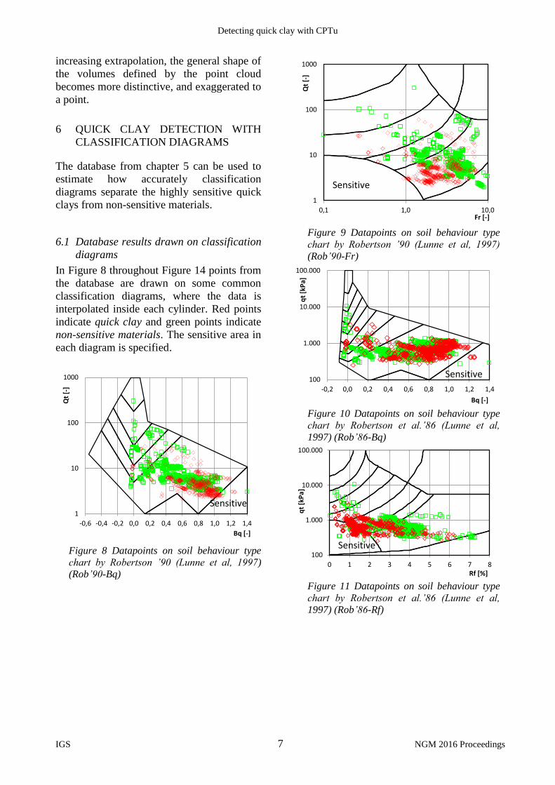
In Figure 8 throughout Figure 14 points from

the database are drawn on some common

classification diagrams, where the data is

interpolated inside each cylinder. Red points

indicate quick clay and green points indicate

non-sensitive materials. The sensitive area in

each diagram is specified.

Figure 8 Datapoints on soil behaviour type

chart by Robertson ’90 (Lunne et al, 1997)

(Rob’90-Bq)


chart by Robertson ’90 (Lunne et al, 1997)

(Rob’90-Fr)


chart by Robertson et al.’86 (Lunne et al,

1997) (Rob’86-Bq)


chart by Robertson et al.’86 (Lunne et al,

1997) (Rob’86-Rf)

1

10

100

1000

-0,6 -0,4 -0,2 0,0 0,2 0,4 0,6 0,8 1,0 1,2 1,4

Qt

[-]

Bq [-]

Sensitive

1

10

100

1000

0,1 1,0 10,0

Qt

[-]

Fr [-]

Sensitive

100

1.000

10.000

100.000

-0,2 0,0 0,2 0,4 0,6 0,8 1,0 1,2 1,4

qt

[kP

a]

Bq [-]

Sensitive

100

1.000

10.000

100.000

0 1 2 3 4 5 6 7 8

qt

[kP

a]

Rf [%]

Sensitive



Figure 12 Datapoints on chart by Senneset et

al.’89 (Eslami et al, 2000) (Sen’89)


chart by Eslami et al., 2000 (Esl’00)


chart by Schneider et al. 2008 (Sch’08)

Table 1 contains the results from the analysis

with no interpolation of the data. It looks as if

methods based on friction have an advantage

over the others when it comes to detecting

presence of sensitive materials, with the

exception of Rob'90-Fr.

Table 1 Summary of classification of sensitive

materials with classification diagrams for the

case of no data interpolation Diagram Quick clay

points classified as quick clay

[%]

Non-sensitive points classified

as quick clay [%]

Esl’00 64,9 10,3

Rob’86-Rf 38,6 8,5

Sch’08 15,2 13,0

Rob’90-Bq 0,6 0,9

Rob’86-Bq 0,6 0,9

Rob’90-Fr 0,0 0,0

Sen’89 0,0 0,0

Every method that correctly identified over

1% of the quick clay datapoints as sensitive

also had a high percentage of false positives.

It should be emphasized that the points used

in this study are taken from 5 test sites, as

shown in Figure 5. It is likely that with a

larger database these results will change.

7 VARIABLES FOR A NEW 3D MODEL

In order to analyze the data in a 3D space the

program MeanCPT has been written (Valsson

2015). The program can present datasets in a

3D space. The axes and scales can be

specified and the model rotated and moved.

Choosing a set of variables for a new model

was done by checking all variables shown in

in chapters 2 and 3 against each axis and

selecting the ones that best divided the

datasets.

The result of this process was that the

variables 𝐵𝑞 (linear-), 𝑓𝑠𝑛 (logarithmic-) and

𝑞𝑡𝑛 (logarithmic scale) would give a good

starting point. The datasets are shown in this

3D space in

Figure 15.

0

2.000

4.000

6.000

8.000

10.000

12.000

14.000

16.000

-0,6 -0,4 -0,2 0,0 0,2 0,4 0,6 0,8 1,0 1,2

qt

[kP

a]

Bq [-]

Sensitive

100

1.000

10.000

100.000

1 10 100 1000

qe [

kPa]

fs [-kPa]

Sensitive

1

10

100

1.000

-2 -1 0 1 2 3 4 5 6 7 8 9 10

Qt

[-]

Δu/σ'v0 [-]

Sensitive



Figure 15 Quick clay and non-sensitive points

viewed in the selected 3D space in MeanCPT.

The view shows the separation of the datasets.

It should be stated that many other variable

combinations were noted as viable candidates

that could also give excellent results.

Using a logarithmic scale on the two axis

helps exaggerate the area/volume in the

model occupied by points of sensitive clay.

8 PROPOSED MODEL

The datasets with the most data (interpolation

between test cylinders) were chosen as a base

for the new model. These sets are shown in

Figure 15.

In order to define the model, points from

areas dominated by non-sensitive materials as

well as from areas where quick and non-

sensitive materials lie close together were

removed. This task was done by hand in

AutoCAD.

This process continued until the model was

little more than a loosely defined volume

defined by an almost entirely red point cloud.

Boundary points were then removed until the

expected false positives of the model, defined

by the imagined bounding volume, were

estimated to be at a minimum.

Figure 16 The resulting quick clay model

shown along with the datasets in MeanCPT.

The volume was defined as a convex hull, and

was created using an automated tool in the

program MeshLab

The model is created directly from datapoints

and is meant to be an example of what is

possible to achieve with this kind of study.

No attempt was made to make any

predictions about areas not defined with data.

The results from the detection process for the

database points are shown in Table 2.

Table 2 Summary of classification with 3D

model for the varying degree of interpolation 3D model Correct

[%] False pos.

[%]

Original data 75,4 6,0

Cylinder interpolation 72,2 7,7

Int. between cylinders 81,3 4,6

It is not surprising that the best results come

from the dataset from which the model was

defined (full interpolation between

cylinders).

When compared to the results in Table 1 it is

apparent that one can expect to get an

increased accuracy for detection of quick

clay of about 10-15%, when compared to the

diagram with the greatest accuracy. If a

penalty is given for false positives this means

an increased accuracy of 15-20%.



The database used to create this model is

however not large enough to create a general

model for quick clay detection.

9 CONCLUSION

The goal of this study is to show that it is

possible to define a 3D model that can detect

quick clay with greater precision than many

2D diagrams in use today.

The classification diagram proposed by

Eslami et al., in 2000 was by far the best 2D

diagram for detecting quick clay. However, it

still had over 10% of points from non-

sensitive materials classified as sensitive

(false positives).

The other 2D diagrams give somewhat

unreliable results when it comes to detecting

sensitive materials and with higher

percentage of correct classification, and some

had more false positives than correct values.

These results can, and likely will, change

with an increased database size.

Out of all tested parameters, the ones chosen

for the resulting model seemed to best

separate quick clay points from points from

non-sensitive materials.

Other parameter sets were observed that

could potentially give good results in a study

like this.

The approach shows potential and merits

further exploration. Increasing the database

size (greatly) should be prioritized in future

work so that a more general model can be

created.

To get more data for such studies the

laboratory setup for samples from CPTu

positions could be modified so that more tests

of the remoulded shear strength are

conducted. These tests should be close to

both ends, as this would aid in the evaluation

of remoulded shear strength variations within

the sample.

If a number of points from a CPTu test are

shown to lie inside the presented model, there

is good reason to be on the lookout for quick

clay in the area.

Files containing 3D model definitions can be

found online, as well as a web-app to check if

any depth intervals within soundings are

classified as quick with this model (Valsson,

2015).

10 REFERENCES

CEN (2012). EN ISO 22476-1:2012: Geotechnical

investigation and testing -- Field testing -- Part 1:

Electrical cone and piezocone penetration test. Comité

Européen Normalisation,

Eslami, A., Fellenius, B.H. (2000): Soil profile

interpreted from CPTu data. “Year 2000

Geotechnics”, Geotechnical Engineering Conference,

Asian Institute of Technology, Bangkok, Thailand,

November 27 - 30, 2000, 18 p.

Gylland A.S. (2015): Utvidet tolkningsgrunnlag

for

Vingebor. Rapport 79/2015. Naturfareprosjektet:

Delprosjekt 6 Kvikkleire (NIFS). Norges vassdrags-

og energidirektorat.

Lunne, T., Robertson, P.K & Powell, J.J.M (1997).

Cone Penetration Testing in Geotechnical Practice. E

& FN Spon, an imprint of Routledge, ISBN 0 419

23750 X.

NGF (2010). Melding nr. 5 - Veiledning for

utførelse av trykksondering. Norsk geoteknisk

forening

NGI (1982): The Rissa landslide, quick clay in

Norway. Video presentation of a famous landslide in

Norway. (https://youtu.be/3q-qfNlEP4A). Norges

Geotekniske Institutt.

Statens vegvesen (2010). Håndbok V220:

Geoteknikk i vegbygging.

Valsson S.M. (2015): MeanCPT.com – Web app

for CPTu data interpretation.

https://youtu.be/3q-qfNlEP4A

Detecting quick clay with CPTu - ngm2016.com · after Begemann in 1965 (from Eslami and Fellenius, 2000) Begemann published the first 0soil profiling chart in 1965 which showed that

Documents