Design of Experiments and Six Sigma

Welcome message from author
This document is posted to help you gain knowledge. Please leave a comment to let me know what you think about it! Share it to your friends and learn new things together.
Transcript

Design of Experiments and Six Sigma

Man’s Quest for Control
Weather Psychology
Engineering
Economy Medicine
Chemistry
Electronics

Input, Environmental and Output Variables of a Process
The Process
State Variables measured here
Ambient temperature, vibration, humidity, supply, voltage, etc. Labor
Training level
Raw materials quality/quantity
Control variables Points for temperature,
cutting speed, raw material specs, recipe,
etc.
Variation in Output Quality of finished Product; Level of
Customer Satisfaction

Lamp
Bulb
Plug Cord
Power
Power outage No house current
Burned out
Loose
Missing
Cord out Not plugged in
No contact
Switch missing
Switch broken
Lamp Doesn’t Turn On
Most effects have a real cause!

Causes and the Effect
Material
Measurements
Methods
Machine
People
Environment
Output Process (Parameters)

B
D O 1 2
3 4
7
5 6
1
8
--- +--
-+- ++-
--+ +-+
We use Design of Experiments to understand and optimize process settings
Perform Experiments Interpret Results
Main Effects Interactions Significance
A B C
Prediction Model Optimize
Reduce Variation Reduce Defects
Y = α + βx1 + αx2 + δx1xs + …

Statistical Techniques in Six Sigma
DOE Regression
Significance Tests Confidence Intervals
X Charts R Charts P Charts np Charts ε Charts ω Charts
Histograms Pareto Charts Cause-and-Effect Tabulating Data
Run Charts Scatter Plots Flow Charts
Six Sigma Black Belts can do these and teach others
About 30% of employees can do these tasks
EVERYBODY can do this

What is an Experiment?
Systematically vary variables of interest e.g. Giving different drugs to subjects In each trial measure the response Critical concepts: • Variable must be manipulated by experimenter • Random assignment of experimental units to conditions • Avoid confounding of variables

Example of a Factor-Response Relationship
45 40 35 30 25 20 15 10 5 0
Seve
rity
of
Can
cer
+
+
+ +
+
+ + +
+ +
0 0.5 1 1.5 2 2.5
# of Packs smoked/day

Correlation
Take two measures from a sample; Calculate correlation coefficient Possible questions: • Is there a relationship between smoking and lung cancer? • Is there a relationship between anxiety and test-taking performance? Correlation does NOT imply causation!

Kinds of Variables
Independent variables (factors) – What you manipulate Dependent variables (responses) – What you measure Control variables – What you hold constant Random (noise) variables – What you allow to vary randomly Confounding variable – Correlated with independent variable

A noisy experiment makes it difficult to find factor effects
100 90 80 70 60 50 40 30 20 10
0
No drug Sugar pill Cocaine Condition
Heart Rate

Example of a well-designed experiment: Factor effects are clearly visible
100 90 80 70 60 50 40 30 20 10
0
No drug Sugar pill Cocaine Condition
Heart Rate

DOE Experiments are Powerful and Efficient – They are Multi-Factorial
Typically, in DOE more than one factor are simultaneously changed. This avoids disadvantages of changing one variable at a time. Changing many factors together brings efficiency by reducing the total number of trials. Changing one factor at a time cannot detect interaction of the effects of two or more factors – a serious fault of one-factor-at-a-time studies. Multi-factorial studies can lead to precise data analysis – ANOVA is the procedure. Changing several factors together can assist in response surface studies and the optimization of the response.

NISSAN Motor Company Supply Chain Problem: Logos won’t stick!
Level Factor
Low High
20 15 Adhesion Area (cm2)
Urethan Acryl Type of glue
Thin Thick Thickness of Foam Styrene
Thin Thick Thickness of Logo
Big Small Amount of pressure
Long Short Pressure application time
No Yes Primer applied
Factors selected for experiments

NISSAN’s DOE Design Array
A – Adhesion Area (cm2) B – Type of Glue C – Thickness of Foam Styrene D – Thickness of Logo
Gluing Str
D C B A No.
9.8 1
8.9 2
9.2 3
8.9 4
12.3 5
13 6
13.9 7
12.6 8
D C B A
5.58 5.65 5.50 4.00 +
5.50 5.43 5.58 5.48 -
Effect Tabulation

Glu
ing
Stre
ngt
h
Adherence Area Type of Glue Thickness of Foam Styrene
Thickness of logo
6.5
4.6
5.58
5.5
5.65
5.43
5.58
5
+ - + - + - + -
Factor Effects Plot

Steps in Planning DOE
1. Define objective 2. Select the Response (Y) 3. Select the Factors (Xs) 4. Choose the factor levels 5. Select the Experimental Design 6. Run Experiment and Collect the Data 7. Analyze the data 8. Conclusions 9. Perform a confirmation run

Advantages of Doing DOE
Statistical foundation of DOE yields a lot of information at relatively low cost. Provides main, secondary and interaction effects of factors being tested. Basic DOE can be conducted and evaluated without significant statistical knowledge or expertise. DOE gives much more information than obtained from one-at-a-time experimentation. DOE – A pro-active tool for directing improvements.

Advantages of Doing DOE (Contd.)
DOE can identify the key decision parameters to control a process and to improve it. In new product/process development historical data are not available; DOE identifies correct levels to help maximize performance and reduce overall costs. DOE can help us reach robust performance; A robust product is insensitive the effect of uncontrollable factors. Factorial experiments are the most economical and precise approach for studying multi-factor effects.

DOE techniques
Full Factorial – The most complete method • 24 = 16 trials • 2 is number of levels • 4 is number of factors Can find Main and Interaction effects. All combinations are tested. Fractional factorial can reduce number of trials from say 16 to 8.
Summary of DOE
DOE is a systematic, rigorous approach to engineering problem-solving. Applies principles and techniques at the data collection stage. Assures the generation of valid, defensible and supportable engineering conclusions. All of this is carried out under the constraint of minimal expenditure of engineering runs, time and money.

Planning for DOE
The motivation for experimentation

Experimental Analysis in Product Realization
DEVELOPMENT
(properties, processes) (concepts, performance)
PRODUCTION
(processes, performance) (monitoring)

Experimentation in Development
What we learn depends on: • Where we look • How we look, and • The scope of our view Resources (people, equipment etc.) Time Material (unprocessed or unusable product)

Experimentation
System
Noise factors
Signal factors Measured response
Control factors
Experimenter’s first goal: Understand the process! Experiments help us study effects of parameters as they are set at various levels.

Cost of Experimentation
Resources (people, equipment etc.) Time Material (unprocessed or unstable product) Usable product that is not being produced

Approaches to Experimentation
1. Build-test-fix problems
2. One-factor-at-a-time (the classical approach)
3. Designed experiments (DOE)

Approaches to Experimentation: Build-Test-Fix
Build-Test-Fix The tinkerer’s approach “Pound it to fit, paint it to match” Impossible to know if true optimum achieved (you quit when it works) Consistently slow: • Requires intuition, luck, rework • Re-optimization and continual fire-fighting

Approaches to Experimentation: One-Factor-at-a-Time
One-factor-at-a-time Procedure (2 level example) • Run all factors at one condition • Repeat, changing condition of one factor • Continuing to hold that factor at that condition, rerun with another
factor at its second condition • Repeat until all factors at their optimum conditions Slow, expensive: Many tests Can miss interactions!

One-Factor-at-a-Time
Process: Yield = f(temperature, pressure)
Max yield: 50% at 78°C, 130 psi? May be not!

One-Factor-at-a-Time
A better view of the maximum yield! By RSM
Process: Yield = f(temperature, pressure)
Major Approaches to using DOE
Factorial Design Taguchi Method Response Surface Design

DOE – Factorial Designs
Full Factorial Simplest design to create but extremely inefficient Each factor tested at each condition of the factor Number of tests, N: N = YX where y = number of conditions, x = number of factors Example: 8 factors, 2 conditions each, N = 28 = 256 tests Results analyzed with ANOVA Cost: Resources, time, materials …

The 23 Factorial Designs
C B A Trial #
Lo Lo Lo 1
Hi Lo Lo 2
Lo Hi Lo 3
Hi Hi Lo 4
Lo Lo Hi 5
Hi Lo Hi 6
Lo Hi Hi 7
Hi Hi Hi 8

Fractional Factorial Designs
Fractional Factorial “less than full” Condition combinations are chosen to provide sufficient information to determine the factor effect. More efficient but risk missing interactions.

Fractional Factorial Designs
(Fractional: 7 factor, 2 level; 128 trials -> to 8)
G F E D C B A Trial
Lo Lo Lo Lo Lo Lo Lo 1
Hi Hi Hi Hi Lo Lo Lo 2
Hi Hi Lo Lo Hi Hi Lo 3
Lo Lo Hi Hi Hi Hi Lo 4
Hi Lo Hi Lo Hi Lo Hi 5
Lo Hi Lo Hi Hi Lo Hi 6
Lo Hi Hi Lo Lo Hi Hi 7
Hi Lo Lo Hi Lo Hi Hi 8

DOE in Response Surface: RSM
Goal: Develop a model that describes a continuous curve, or surface, that connects the measured data taken at strategically important places in the experimental window.

DOE in Response Surface: RSM
RSM uses a least-squares curve-fit (regression analysis) to: Calculate a system model (what is the process?) Tests its validity (does it fit?) Analyze the model (how does it behave?)
Bond – f(temperature, pressure, duration) Y = a0 + a1T + a2P + a3D + a11T2 + a22P2 + a33D2
+ a12TP + a13TD + a23PD

Illustrating the DOE Process
1. Determine the goals 2. Define the measures of success 3. Verify feasibility (rough estimate) 4. Design the experiment (precise estimate) 5. Run the experiment 6. Collect and analyze the data 7. Determine and verify the response 8. Act on the results

Experimental Design Process
1. Determine the goals
Doing so often leads to: • Goals are too many to cover in a single study • Goals that seemed concrete are actually very negotiable Once consensus is achieved, a valid experimentation strategy can be developed. Plan the action to be taken if the experiment is a success or a failure.

Experimental Design Process
2. Define the measures of success Once the goals are set, how do we know when we are meeting them? Measures must be metric and refer to an intrinsic feature of the process of product. • Qualitative “good/bad” cannot be modeled Include a large number of responses just to see how they change often diverts focus from the responses that are critical to meeting the goals.

Experimental Design Process
3. Verify feasibility (rough estimate)
Use a power calculation to determine whether any information can be found with a reasonable number of trials. A function of the amount of noise associated with a response. The more noise in the process, the more trials required to see a change in the desired parameter.

Experimental Design Process
3. Verify feasibility (rough estimate) Example: How many runs needed to observe changes of 5,000 psi in the tensile strength of a plastic extruded part?
Number of runs Resolution (psi)
5 10,000
22 5,000
90 2,500
362 1,250

Experimental Design Process
4. Design the experiment (precise estimate) Identify the controls to be varied. Make the design. Determine whether the number of experiments is too large. If necessary, use a screening design to sift through to find the critical few influencing factors.

Experimental Design Process
5. Run the experiment A task in resource management. Complete the work as efficiently and as effectively as possible.

Experimental Design Process
6. Collect and analyze the data Best to examine the data as a whole. Analysis of a set of data has significant advantage over contrasting the results between two data points. • Ability to find suspect data is greatly enhanced. If there is a choice as to order, you may wish to obtain the most critical data first.

Experimental Design Process
7. Determine and verify the response A Response Surface give you the ability to predict, with statistical limits, the behavior of the process at any point within the design window. Combining predictions from several responses allows you to simultaneously optimize for several key specifications.
Experimental Design Process
8. Act on the results Goals set earlier identified what was to be done if success obtained – Do it! If no action is taken why was the experiment done? Complete the documentation of the experiment.

Considerations
The cost of experimentation • Resources (people, equipment etc.) • Time • Material (unprocessed or unusable product) • Usable product that is not being produced Experimenter’s foremost goal: Understand the process!

Approaches
Approaches to experimentation • Build-test-fix • One-factor-at-a-time (the conventional approach) • Designed experiments (DOE) Major approaches to DOE: • Factorial Design (full, fractional) • Taguchi Method • Response Surface Design

Other Approaches
Full factorial • Simplest design to create but extremely inefficient • Each factor tested at each condition of the factor • Results analyzed with ANOVA • Cost: Resources, time, materials Taguchi Method • Taguchi designs created before desktop computers were
common. • Designs cannot support response surface models and are
limited to only predicting at the points where data was taken.

Summary
Experimental Design process steps: • Determine the goals • Define the measures of success • Verify feasibility (rough estimate) • Design the experiment (precise estimate) • Run the experiment • Collect and analyze the data • Determine and verify the response • Act on the results

An Important Application of DOE: Taguchi Methods

Genichi Taguchi
An engineer who developed an approach (now called Taguchi Methods) involving statistically planned experiments to reduce variation in quality. Learned DOE from Professor Rao. In 1960’s he applied his learning in Japan. In 1980’s he introduced his ideas to US and AT&T.

C. R. Rao
You’d know Rao from his Cramer-Rao Inequality. Rao is recognized worldwide as a pioneer of modern multivariate theory and as one of the world’s top statisticians, with distinctions as a mathematician, researcher, scientist and teacher. Taught Taguchi. Author of 14 books and over 300 papers.

What are Taguchi’s Contributions?
Quality Engineering Philosophy Methodology Efficient Experiment Design scheme Simple Analysis
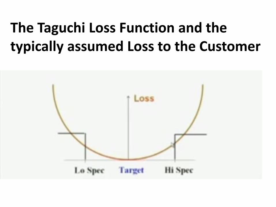
The Taguchi Loss Function and the typically assumed Loss to the Customer

Taguchi’s Quality Philosophy
On target production is more important than producing within Specs
Loss = k(P – T)2
Not 0 if within specs and 1 if outside
Taguchi’s view Conventional view

Robust Design
Robust Design: Design that results in products or services that can function over a broad range of usage and environmental conditions.

Conventional DOE focuses only on Average Response FACTOR LOW (-) HIGH (+) D (Driver) regular oversized B (Beverage) beer water O (Ball) 3-piece balanta
Avg Response
O B D Standard Order
67 - - - 1
79 - - + 2
61 - + - 3
75 - + + 4
65 + - - 5
60 + - + 6
77 + + - 7
87 + + + 8
QE focuses on Variability of Response
77 87
61 75
65 60
67 79
B
D
O
B
D O 1 2
3 4
7
5 6
1
8
--- +--
-+- ++-
--+ +-+
-++ +++

Robust Design – How it is done
Identify Product/Process Design Parameters that: • Have significant/little influence on performance • Minimize performance variation due to noise factors • Minimize the processing cost Methodology: Design of Experiments (DOE) Examples: Chocolate mix, Ina Tile Co., Sony TV
Target Performance Product/Process
Design Parameters (D)
Actual Performance (P)
Noise Factors (N), Internal & External

DOE in Taguchi Method
Taguchi experimental designs were created before desktop computers were common: Pre-created, cataloged designs intended to quickly find a set of conditions that meet the criteria of success Previous slide an example of an L8 template Designs cannot support response surface models and are limited to only predicting at the points where data was taken.

Full Factorial Array Example: The 23 (8-trial) array
A B
C
7 6 5 4 3 2 1
1 1 1 1 1 1 1
2 2 2 2 1 1 1
2 2 1 1 2 2 1
1 1 2 2 2 2 1
2 1 2 1 2 1 2
1 2 1 2 2 1 2
1 2 2 1 1 2 2
2 1 1 2 1 2 2
Full Factorial Factor Assignments to Experimental Array Columns. Such experiments can find all Main and two- and three-factor interactions.
C B -BC A -AC -AB -ABC
Array Columns
Response

Taguchi’s Orthogonal Designs vs. Classical DOE
Column no
7 6 5 4 3 2 1 Run
1 1 1 1 1 1 1 1
2 2 2 2 1 1 1 2
2 2 1 1 2 2 1 3
1 1 2 2 2 2 1 4
2 1 2 1 2 1 2 5
1 2 1 2 2 1 2 6
1 2 2 1 1 2 2 7
2 1 1 2 1 2 2 8
Classical col no C B BC A AC AB ABC
Taguchi L8 Array

Taguchi’s Robust Design Experiments
Taguchi advocated using inner and outer array designs to take into account noise factors (outer) and design factors (inner) Design factors: I 1, I 2, I 3
Noise factors: E 1 and E 2
Objective: Maximize response while minimizing its variance
I 1
I 2 I 3
E 1
E 2
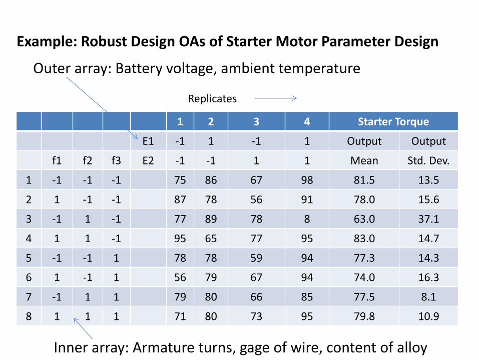
Example: Robust Design OAs of Starter Motor Parameter Design
Starter Torque 4 3 2 1
Output Output 1 -1 1 -1 E1
Std. Dev. Mean 1 1 -1 -1 E2 f3 f2 f1
13.5 81.5 98 67 86 75 -1 -1 -1 1
15.6 78.0 91 56 78 87 -1 -1 1 2
37.1 63.0 8 78 89 77 -1 1 -1 3
14.7 83.0 95 77 65 95 -1 1 1 4
14.3 77.3 94 59 78 78 1 -1 -1 5
16.3 74.0 94 67 79 56 1 -1 1 6
8.1 77.5 85 66 80 79 1 1 -1 7
10.9 79.8 95 73 80 71 1 1 1 8
Outer array: Battery voltage, ambient temperature
Replicates
Inner array: Armature turns, gage of wire, content of alloy

S/N Ratios are Maximized
𝑆𝑁𝑧 = 10log(𝑦2
𝑠2)
𝑆𝑁𝑧 = −10log( 1/𝑦2
𝑛)
𝑆𝑁𝑧 = −10log( 𝑦2
𝑛)
To maximize robustness, when Target performance is the best, Taguchi uses the signal-to-noise ratio
When response is to be maximized, Taguchi uses
When response is to be minimized, Taguchi uses
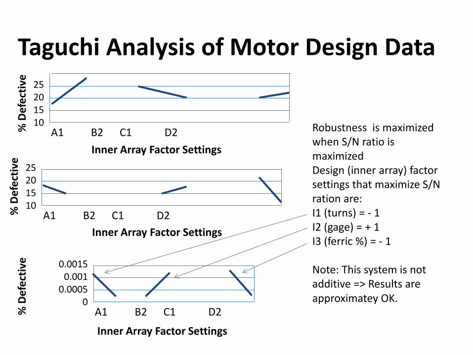
Taguchi Analysis of Motor Design Data
Robustness is maximized when S/N ratio is maximized Design (inner array) factor settings that maximize S/N ration are: I1 (turns) = - 1 I2 (gage) = + 1 I3 (ferric %) = - 1 Note: This system is not additive => Results are approximatey OK.
Inner Array Factor Settings
% D
efe
ctiv
e
25 20 15 10
A1 B2 C1 D2
Inner Array Factor Settings
% D
efe
ctiv
e
25 20 15 10
A1 B2 C1 D2
Inner Array Factor Settings
% D
efe
ctiv
e
0.0015 0.001
0.0005 0
A1 B2 C1 D2
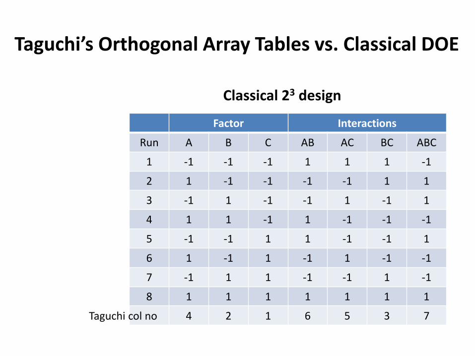
Taguchi’s Orthogonal Array Tables vs. Classical DOE
Classical 23 design
Interactions Factor
ABC BC AC AB C B A Run
-1 1 1 1 -1 -1 -1 1
1 1 -1 -1 -1 -1 1 2
1 -1 1 -1 -1 1 -1 3
-1 -1 -1 1 -1 1 1 4
1 -1 -1 1 1 -1 -1 5
-1 -1 1 -1 1 -1 1 6
-1 1 -1 -1 1 1 -1 7
1 1 1 1 1 1 1 8
7 3 5 6 1 2 4 Taguchi col no

Taguchi Orthogonal Array Tables
2-level (fractional factorial) arrays: L4(23). L8(27). L16(215). L32(231). L64(263) 2-level arrays: L12(211) (Plackett-Burman Design) 3-level arrays: L9(34). L27(33). L81(340) 4-level arrays: L16(45). L64(421) 5-level arrays: L25(56) Mixed-level arrays: L15(21 X 37), L32(21 X 49), L50(21 X 511)

Response Surface Methods
Conducting optimization through experiments
Related Documents


