Struct Multidisc Optim (2012) 45:65–81 DOI 10.1007/s00158-011-0657-4 RESEARCH PAPER Design of conjugate, conjoined shapes and tilings using topology optimization M. Meenakshi Sundaram · Padmanabh Limaye · G. K. Ananthasuresh Received: 11 March 2010 / Revised: 17 February 2011 / Accepted: 11 April 2011 / Published online: 28 May 2011 c Springer-Verlag 2011 Abstract We present a method for obtaining conjugate, conjoined shapes and tilings in the context of the design of structures using topology optimization. Optimal mate- rial distribution is achieved in topology optimization by setting up a selection field in the design domain to deter- mine the presence/absence of material there. We generalize this approach in this paper by presenting a paradigm in which the material left out by the selection field is also utilised. We obtain conjugate shapes when the region cho- sen and the region left-out are solutions for two problems, each with a different functionality. On the other hand, if the left-out region is connected to the selected region in some pre-determined fashion for achieving a single functionality, then we get conjoined shapes. The utilization of the left-out material, gives the notion of material economy in both cases. Thus, material wastage is avoided in the practical realiza- tion of these designs using many manufacturing techniques. This is in contrast to the wastage of left-out material dur- ing manufacture of traditional topology-optimized designs. We illustrate such shapes in the case of stiff structures and An enhanced version of a brief conference paper presented at the World Conference of Structural and Multi-disciplinary Optimization 2009, titled ‘Optimal conjugate topologies on a single domain’, by Padmanabh Limaye, M. Meenakshi Sundaram, and G. K. Ananthasuresh. M. Meenakshi Sundaram (B ) · P. Limaye · G. K. Ananthasuresh Department of Mechanical Engineering, Indian Institute of Science, Bangalore, India e-mail: [email protected] P. Limaye e-mail: [email protected] G. K. Ananthasuresh e-mail: [email protected] compliant mechanisms. When such designs are suitably made on domains of the unit cell of a tiling, this leads to the formation of new tilings which are functionally useful. Such shapes are not only useful for their functionality and economy of material and manufacturing, but also for their aesthetic value. Keywords Material economy · Symmetry · Interlocking · Conjugate · Conjoined · Tilings · Topology optimization · Compliant mechanisms 1 Introduction Topology optimization is a technique to solve a material distribution problem wherein a given amount of material is distributed optimally to achieve an objective while sat- isfying some constraints. To illustrate this, we consider the problem of minimization of the strain energy, which is a measure of stiffness of a structure made of an elastic material. min ρ 1 2 (u) T : D(ρ) : (u)d (1) subject to ∇ · ( D(ρ) : ) + F = 0 ( D(ρ) : ) n = t on ∂ t u = u s on ∂ u (2) ρ d ≤ V ∗ (3) 0 ≤ ρ ≤ 1 (4)

Welcome message from author
This document is posted to help you gain knowledge. Please leave a comment to let me know what you think about it! Share it to your friends and learn new things together.
Transcript

Struct Multidisc Optim (2012) 45:65–81DOI 10.1007/s00158-011-0657-4
RESEARCH PAPER
Design of conjugate, conjoined shapes and tilings using topologyoptimization
M. Meenakshi Sundaram · Padmanabh Limaye ·G. K. Ananthasuresh
Received: 11 March 2010 / Revised: 17 February 2011 / Accepted: 11 April 2011 / Published online: 28 May 2011c© Springer-Verlag 2011
Abstract We present a method for obtaining conjugate,conjoined shapes and tilings in the context of the designof structures using topology optimization. Optimal mate-rial distribution is achieved in topology optimization bysetting up a selection field in the design domain to deter-mine the presence/absence of material there. We generalizethis approach in this paper by presenting a paradigm inwhich the material left out by the selection field is alsoutilised. We obtain conjugate shapes when the region cho-sen and the region left-out are solutions for two problems,each with a different functionality. On the other hand, if theleft-out region is connected to the selected region in somepre-determined fashion for achieving a single functionality,then we get conjoined shapes. The utilization of the left-outmaterial, gives the notion of material economy in both cases.Thus, material wastage is avoided in the practical realiza-tion of these designs using many manufacturing techniques.This is in contrast to the wastage of left-out material dur-ing manufacture of traditional topology-optimized designs.We illustrate such shapes in the case of stiff structures and
An enhanced version of a brief conference paper presented at theWorld Conference of Structural and Multi-disciplinary Optimization2009, titled ‘Optimal conjugate topologies on a single domain’, byPadmanabh Limaye, M. Meenakshi Sundaram, and G. K.Ananthasuresh.
M. Meenakshi Sundaram (B) · P. Limaye · G. K. AnanthasureshDepartment of Mechanical Engineering, Indian Institute of Science,Bangalore, Indiae-mail: [email protected]
P. Limayee-mail: [email protected]
G. K. Ananthasureshe-mail: [email protected]
compliant mechanisms. When such designs are suitablymade on domains of the unit cell of a tiling, this leads tothe formation of new tilings which are functionally useful.Such shapes are not only useful for their functionality andeconomy of material and manufacturing, but also for theiraesthetic value.
Keywords Material economy · Symmetry · Interlocking ·Conjugate · Conjoined · Tilings · Topology optimization ·Compliant mechanisms
1 Introduction
Topology optimization is a technique to solve a materialdistribution problem wherein a given amount of materialis distributed optimally to achieve an objective while sat-isfying some constraints. To illustrate this, we considerthe problem of minimization of the strain energy, whichis a measure of stiffness of a structure made of an elasticmaterial.
minρ
1
2
∫�
ε(u)T : D(ρ) : ε(u)d� (1)
subject to
∇ · (D(ρ) : ε) + F = 0
(D(ρ) : ε) n = t on ∂�t
u = us on ∂�u (2)
∫�
ρd� ≤ V ∗ (3)
0 ≤ ρ ≤ 1 (4)
66 M. Meenakshi Sundaram et al.
In the functional to be minimized in (1) and the equilib-rium equation of (2), ε = 1
2
(∇u + ∇uT)
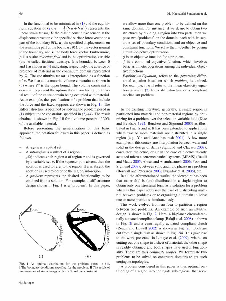
represents thelinear strain tensor, D the elastic constitutive tensor, u thedisplacement vector, t the specified surface force vector on apart of the boundary ∂�t , us the specified displacements onthe remaining part of the boundary ∂�u , n the vector normalto the boundary, and F the body force vector. Furthermore,ρ is a scalar selection field and is the optimization variable(the so-called fictitious density). It is bounded between 0and 1 as shown in (4) indicating, respectively, the absence orpresence of material in the continuum domain representedby �. The constitutive tensor is interpolated as a functionof ρ. We also add a material volume constraint as shown in(3) where V ∗ is the upper bound. The volume constraint isessential to prevent the optimization from taking up a triv-ial result of the entire domain being occupied with material.As an example, the specifications of a problem that includethe force and the fixed supports are shown in Fig. 1i. Thestiffest structure is obtained by solving the problem posed in(1) subject to the constraints specified in (2)–(4). The resultobtained is shown in Fig. 1ii for a volume percent of 30%of the available material.
Before presenting the generalization of this basicapproach, the notation followed in this paper is defined asfollows.
– A region is a spatial set.– A sub-region is a subset of a region.– ρ�b
a indicates sub-region b of region a and is governedby a variable set ρ. If the superscript is absent, then thenotation is used to refer to the region. If ρ is absent, thenotation is used to describe the region/sub-region.
– A problem represents the desired functionality to beobtained from a solution. For example, a stiff structuredesign shown in Fig. 1 is a ‘problem’. In this paper,
Fig. 1 An optimal distribution for the problem posed in (1).i The boundary conditions specified for the problem. ii The result ofminimization of strain energy with a 30% volume constraint
we allow more than one problem to be defined on thesame domain. For instance, if we desire to obtain twostructures by dividing a region into two parts, then wepose two ‘problems’ on the domain, each with its sep-arate set of boundary conditions and an objective andconstraint functions. We solve them together by posinga multi-objective optimization.
– φ is an objective function for a problem.– f is a combined objective function, which involves
basic arithmetic operations among the individual objec-tive functions.
– Equilibrium Equationi refers to the governing differ-ential equation based on which problemi is defined.For example, it will refer to the linear elasticity equa-tion given in (2) for a stiff structure or a compliantmechanism problem.
In the existing literature, generally, a single region ispartitioned into material and non-material regions by opti-mizing for a problem over the selection variable field (Diazand Bendsøe 1992; Bendsøe and Sigmund 2003) as illus-trated in Fig. 1i and ii. It has been extended to applicationswhere two or more materials are distributed in a singleregion (e.g., Yin and Ananthasuresh 2001). A few moreexamples in this context are interpolation between water andsolid in the design of dams (Sigmund and Clausen 2007);conductor, dielectric, or air in the case of electrostaticallyactuated micro electromechanical systems (MEMS) (Raulliand Maute 2005; Alwan and Ananthasuresh 2006; Yoon andSigmund 2008); between solid and fluid phases in a problem(Borrvall and Petersson 2003; Evgrafov et al. 2006), etc.
In all the aforementioned works, the viewpoint has beenthat material(s) is (are) distributed in a single region toobtain only one structural form as a solution for a problemwhereas this paper addresses the case of distributing mate-rial between problems or re-organising a domain to solveone or more problems simultaneously.
This work evolved from an idea to partition a regionbetween two problems. An example of such an intuitivedesign is shown in Fig. 2. Here, a bi-planar circumferen-tially actuated compliant clamp (Balaji et al. 2008) is shownin Fig. 2i and a centrifugally actuated compliant clutch(Roach and Howell 2002) is shown in Fig. 2ii. Both arecut from a single disk as shown in Fig. 2iii. This gave riseto the work presented in Limaye et al. (2009), where, oncutting out one shape in a sheet of material, the other shapeis readily obtained and both shapes have useful function-ality. These are thus conjugate shapes. We formulate twoproblems to be solved on congruent domains to get suchconjugate topologies.
A problem considered in this paper is thus optimal par-titioning of a region into conjugate sub-regions, that serve

Conjugate, conjoined shapes and tilings 67
Fig. 2 Two conjugate compliant mechanisms snugly fitting in a circu-lar disk. i A bi-planar circumferentially actuated clamp. ii A centrifugalclutch. iii Both mechanisms placed together to show their conjugateshapes
different functionalities for different problems but are cre-ated out of a single manufacturing operation. When twoconjugate shapes are obtained by cutting out a regionthere is no wastage of material in many manufacturingtechniques. Milling, water-jet cutting, laser machining,lithography, blanking and punching, and other planar man-ufacturing processes gain from such designs. In particular,in micromachined structures made with silicon, the areaon the chip is very valuable because of the high process-ing cost incurred in batch-processing. On the other hand,it is worth noting that left-out material is wasted in tra-ditional topology-optimized designs during manufacturing.The same applies to the manufacture of moulds in casting,moulding, extrusion, etc.
Another extension of topology design presented in thepaper is to re-arrange material in a sub-region over theentire region to solve one problem. A practical applicationof this technique is found in castellated beams as describedin Knowles (1991). It is an ingenious design in which theweb of an I-beam is cut along the dashed line as shownin Fig. 3i and then re-attached as shown in Fig. 3ii toincrease its depth and thereby increase its bending stiffness.We call such designs conjoined designs. These designs,although not necessarily optimal for the material that theyutilize, have a conjugate symmetry built into them that leadsto manufacturing economy as once again no material iswasted.
The idea of conjoining, as described above, motivated usto partition or re-organise existing tileable geometries so asto get new tiles which are functionally useful. Such designspresented in an artistic context are seen in the works of M. C.Escher of which an example is shown in Fig. 4. An optimaltileable geometrical form gives material economy for themanufacturing processes mentioned earlier.
At this juncture, we would like to underscore the depar-ture from conventional paradigm for topology optimization.Conventionally, the focus is on distributing a given amountof material to obtain one functionality without botheringabout the material left out in the domain. On the contrary,the aforementioned examples illustrate cases where the
(i) Uncut Beam
(ii) Castellated Beam
Fig. 3 Construction of the castellated beams. i The original I-beamwith the markings along which the cut is to be made. ii The cut andre-assembled portions of the beam
entire material of a region/sub-region is used in achievingthe objective comprising single or multiple functionalities.
The following section of this paper discusses the parame-terization and formulation for obtaining conjugate and con-joined shapes. This is the main contribution of this paper.After this, we present the numerical algorithm that was usedto perform the optimization. Following this, the results withrespect to stiff structures and compliant mechanisms arediscussed, with some manufacturing details presented there-after. Some examples related to the special case of tilingsare also presented. Next, generalizations of these conceptsto obtain multiple conjugate shapes is presented. Finally, afew concluding remarks and some ideas for future work arenoted.
Fig. 4 A tiling obtained from a prototile of a horse and its rider(adapted from M. C. Escher’s paintings)

68 M. Meenakshi Sundaram et al.
2 Design parameterization and problem formulation
Design parameterization is the crucial aspect of this work.Therefore, in this section, we address and motivate the man-ner in which the selection field is setup across and within aregion to obtain conjugate and conjoined designs. We alsopresent an example of a problem statement for each of theproblem situations considered in this paper.
2.1 Conjugate shapes
As mentioned in Section 1, the objective is to obtain twodesigns from a single region leaving no material unused. Todo so, we consider two congruent regions ρ�1 and ρc�2 asshown in Fig. 5. The selection field is chosen to be ρ onone of them and 1 − ρ (denoted by ρc) on the other, anda problem is posed on each of these regions. The idea isthat material not selected in one region is to be utilized bythe other. This enables both problems to utilize the entiredomain. An example of a possible design that we wouldwant is illustrated in Fig. 5. A problem statement for this isgiven by
minρ
f ( φ1︸︷︷︸ρ�1
, φ2︸︷︷︸ρc �1
) (5)
subject to
Equilibrium Equation1 on ρ�1
Equilibrium Equation2 on ρc�1
0 ≤ ρ ≤ 1
The notation φ1︸︷︷︸ρ�1
indicates that the objective function φ1
is defined over the region and scalar selection field given by
ρ�1. The function f (φ1, φ2) in (5) may involve any arith-metic combination of individual objective functions, φ1 andφ2, depending on the problem being solved. For example,if we need to minimise φ1 and maximise φ2, then we cancouple them as f = φ1
φ2which is to be minimized.
Fig. 5 A schematic of the design parameterization to obtain conjugateshapes with a depiction of a possible design
2.2 Conjoined shapes
As opposed to conjugate shapes, here, the goal is to achievea single design from a combination of two congruent sub-regions and completely utilizing the material in a singlesub-region. To understand this, consider a region �1 com-prising two congruent sub-regions �1
1 and �21 as shown in
Fig. 6i. Note that �21 is a sub-region obtained by rotating
�11 by 180◦ The selection field on �1
1 is chosen to be ρ
and on �21 is chosen to be ρc as shown in Fig. 6ii. Now,
a problem is posed on the conjoined domain with a possibledesign shown as the shaded portion in Fig. 6iii. A problemstatement for this is as follows:
minρ
φ︸︷︷︸�1
(6)
subject to
Equilibrium Equation on �1
0 ≤ ρ ≤ 1
where
�1 = ρcrot
�21
⋃ρ�1
1
ρcrot = (1 − ρ) rotated by 180◦
As in conjugate shapes, here too, we want the materialof a sub-region to be completely utilized. The differencehere is that the material cut out from ρ�1
1, i.e., the unshaded
(i)
(ii)
(iii)
Fig. 6 A schematic of the design parameterization to obtain conjoinedshapes when the congruent sub-regions are i rotated and then ii joinedtogether, with iii a depiction of a possible design

Conjugate, conjoined shapes and tilings 69
part is joined using a predetermined transformation with itto make a bigger new structural form. The castellated beamdiscussed in Section 1 (see Fig. 3) is an example that showsthe practical use of this concept.
3 Numerical algorithm
The numerical algorithm shown in Fig. 7 follows the linesof the standard topology optimization algorithm (Bendsøeand Sigmund 2003), where we use finite element analysis(FEA) to solve the equilibrium equations, and then evaluatethe objective and constraint functions, and their gradients.Here, the selection field ρ is discretized so that it is con-stant over each element of the mesh but varies across theelements. The Young’s modulus is interpolated by SIMP(Solid Isotropic Material with Penalization) as E = E1ρ
3.The value of ρ being zero or one will yield a zero for theYoung’s modulus in the region governed by ρ or 1 − ρ,respectively. This translates to a singularity of the stiffnessmatrix. Hence, as common in this technique, we chooselower and upper bounds on ρ to be 0.001 and 0.999.
Topology optimization warrants spatial filtering in orderto avoid checker-board and one-node hinge patterns and todecrease mesh-dependency in the finite element framework.The algorithm has a slight difference when using one orthe other. In the forthcoming sub-section we will presenttwo filtering schemes, namely, the sensitivity filter and thedensity filter which are both used in topology optimization(Sigmund 2007). We will also explain why density filteringis better suited for the problems considered in this paper.
If the sensitivity filter is used as shown in Fig. 7i, thenevery iteration proceeds with the allocation of the variablesand its complement to the respective regions or sub-regions.This is followed by the analysis and sensitivity computa-tions. These sensitivities are then filtered and used to makethe optimality criteria update.
On the other hand if the density filter is used as shown inFig. 7ii, then every iteration begins with the filtering of thevariables. This is followed by the allocation of the filteredvariables and its complement to the respective regions orsub-regions. Now the function is evaluated and the gradientswith respect to the actual variables (not the filtered ones) arecomputed. This is followed by an optimality criteria update.
Fig. 7 Flowcharts of thenumerical algorithm using:i sensitivity filtering. ii densityfiltering
70 M. Meenakshi Sundaram et al.
The iterations are stopped when the relative changebetween the successive sets of variables is lower than thetolerance value, i.e., ||ρ−ρold||2||ρ||2 < tol. In the following sub-sections we will be discussing two aspects, namely, filteringand the optimality criteria method.
3.1 Filtering
The sensitivity filter proposed by Sigmund (2001) is givenby
∂̂φ
∂ρ
∣∣∣∣e
=
∑p∈Se
ρp Hp∂φ
∂ρ
∣∣∣∣p
ρe
∑p∈Se
Hp
(7)
where
Hp = r − dist (e, p)
Se = {p|dist (e, p) < r}
Here, the symbol e refers to the element in the finite ele-ment mesh under consideration and dist (e, p) refers to theEuclidean distance between the centroids of elements e andp. Further, Se refers to the region of influence prescribed byr , the radius of the filter around element e.
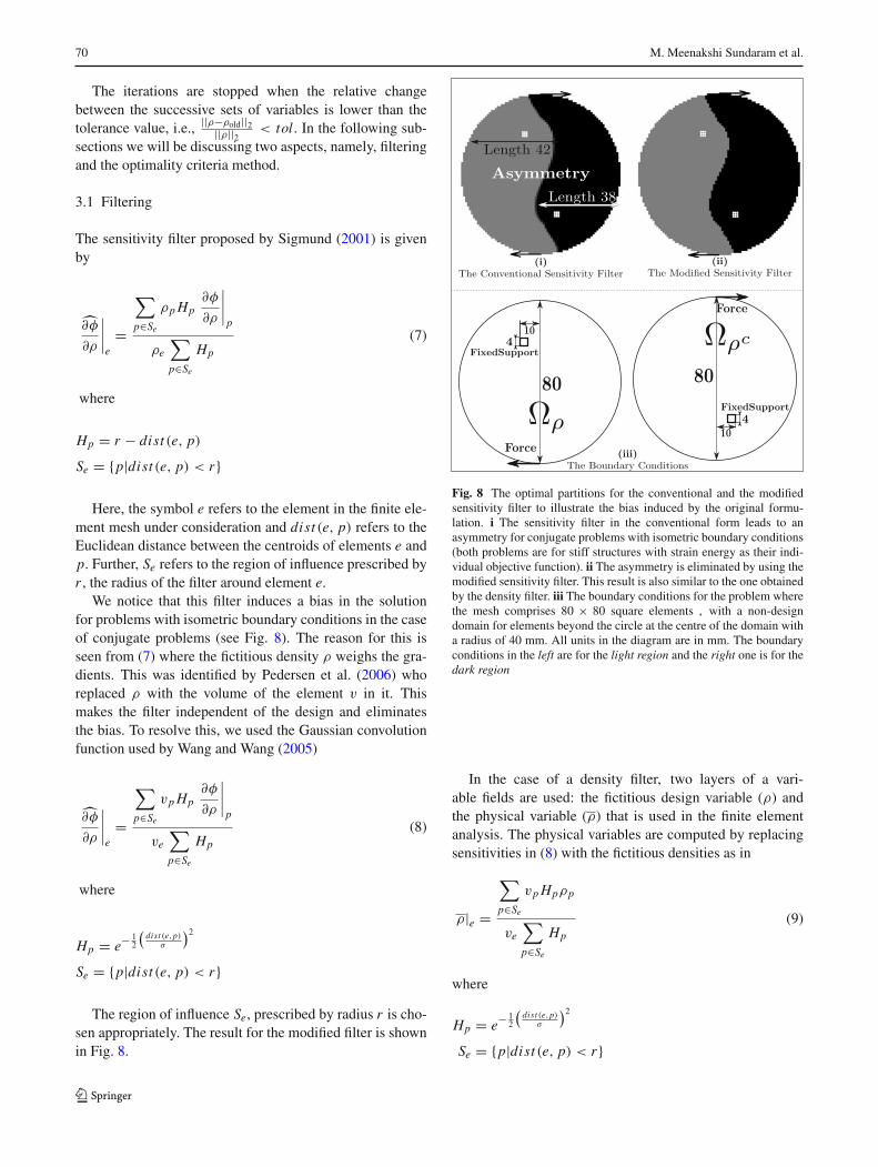
We notice that this filter induces a bias in the solutionfor problems with isometric boundary conditions in the caseof conjugate problems (see Fig. 8). The reason for this isseen from (7) where the fictitious density ρ weighs the gra-dients. This was identified by Pedersen et al. (2006) whoreplaced ρ with the volume of the element v in it. Thismakes the filter independent of the design and eliminatesthe bias. To resolve this, we used the Gaussian convolutionfunction used by Wang and Wang (2005)
∂̂φ
∂ρ
∣∣∣∣e
=
∑p∈Se
vp Hp∂φ
∂ρ
∣∣∣∣p
ve
∑p∈Se
Hp
(8)
where
Hp = e− 12
(dist (e,p)
σ
)2
Se = {p|dist (e, p) < r}
The region of influence Se, prescribed by radius r is cho-sen appropriately. The result for the modified filter is shownin Fig. 8.
Fig. 8 The optimal partitions for the conventional and the modifiedsensitivity filter to illustrate the bias induced by the original formu-lation. i The sensitivity filter in the conventional form leads to anasymmetry for conjugate problems with isometric boundary conditions(both problems are for stiff structures with strain energy as their indi-vidual objective function). ii The asymmetry is eliminated by using themodified sensitivity filter. This result is also similar to the one obtainedby the density filter. iii The boundary conditions for the problem wherethe mesh comprises 80 × 80 square elements , with a non-designdomain for elements beyond the circle at the centre of the domain witha radius of 40 mm. All units in the diagram are in mm. The boundaryconditions in the left are for the light region and the right one is for thedark region
In the case of a density filter, two layers of a vari-able fields are used: the fictitious design variable (ρ) andthe physical variable (ρ) that is used in the finite elementanalysis. The physical variables are computed by replacingsensitivities in (8) with the fictitious densities as in
ρ|e =
∑p∈Se
vp Hpρp
ve
∑p∈Se
Hp
(9)
where
Hp = e− 12
(dist (e,p)
σ
)2
Se = {p|dist (e, p) < r}

Conjugate, conjoined shapes and tilings 71
Then, the chain rule is used to compute the sensitivities asin
∂φ
∂ρ
∣∣∣∣e
=∑p∈Se
∂φ
∂ρ
∣∣∣∣p
∂ρ p
∂ρe
∂ρ p
∂ρe= ve He
vp
∑i∈Sp
Hi
(10)
where, the terms r , e, and Se have the same meaning as inthe case of the sensitivity filter. The result for this techniqueis similar to the one shown in Fig. 8ii for the same boundaryconditions.
In the density filtering technique, one must render thephysical variables and hence there will be a gray interfacebetween the black and white regions even at convergence.On the other hand, the sensitivity filter has a clear interface.More importantly, the density filtering technique providesgradients that are equal to the actual gradients of the objec-tive function and the constraint while the sensitivity filter-ing technique does not. Consequently, better convergencebehaviour is seen with the density filter than with the sensi-tivity filter for the type of problems considered in this paper.Hence, the results presented hereafter use the density filter.
3.2 Optimality criteria method
Although any nonlinear programming technique can be usedto solve problems posed in this paper, we found it conve-nient to use the optimality criteria method. The optimizationproblems posed in this paper do not involve any constraintsother than the box constraints that limit ρ between 0 and 1.Therefore, the optimality criterion implies that the gradientof the objective function is zero. Hence, we formulated theupdate scheme as follows.
ρnew =⎧⎨⎩
Min if U pdate ≤ MinUpdate if Min ≤ U pdate ≤ MaxMax if Max ≤ U pdate
(11)
where
B = ∂φ
∂ρ
1
Scale(12)
Min = max(ρmin, ρ − m) (13)
Max = min(1 − ρmin, ρ + m) (14)
Update = ρ(1 − sign(B)|B|η) (15)
The constants η and m are the damping term and the move
limit, respectively. The absolute value of the gradient is usedto avoid imaginary values when it is raised to the power
of η. The sign function captures the direction intended bythe gradient. The Scale value, chosen to be of the order ofthe gradients of the initial guess, stabilizes the algorithm.The quantity (1 − sign(B)|B|η) in (15), which multiplies ρ,approaches 1 as the gradient of φ tends to zero. The valuesof ρmin and ρmax are 0.001 and 0.999, as mentioned before.
When this was implemented, we found that there wasa slight bias towards one of the problems in the case ofisometric boundary conditions. We attribute this to theround-off errors. To avoid this, we updated the fictitiousdensity ρc also by using the same scheme and averaged outthe result as shown next.
ρcnew =
⎧⎨⎩
Min if U pdate ≤ MinUpdate if Min ≤ U pdate ≤ MaxMax if Max < U pdate
(16)
where
B = −∂φ
∂ρ
1
Scale
ρcmin = ρmin ρc
max = ρmax
Min = max(ρc
min, ρc − m
)Max = min
(1 − ρc
min, ρc + m
)
Update = ρc(1 − sign(B)|B|η)
ρavg = ρnew + (1 − ρc
new
)2
4 Results and discussion
In this section, we discuss the examples presented in eachof the cases, viz., conjugate shapes, conjoined shapes,and the special cases of tilings. The results obtained per-tain to stiff structures and compliant mechanisms. For thestiff structures, we minimize the strain energy of the struc-ture (Bendsøe and Kikuchi 1988). On the other hand,for compliant mechanism, we maximize MSE
SE (Saxena andAnanthasuresh 2000). MSE stands for the mutual strainenergy and is numerically equal to the displacement at theoutput of the mechanism along the desired direction. Anoutput spring is used to obtain connected structures in com-pliant mechanisms (Deepak et al. 2009). Here, the term SErefers to the strain energy of the spring and the compliantmechanism taken together. In all the examples, we used aPoisson’s ratio of 0.3 and Young’s modulus = 1 N/m2. Itmust be noted that the Young’s modulus was scaled to unityto maintain objective function values suitable for the opti-mization routine. This scaling does not affect the optimalshape. However, the strain energy and other terms need to
72 M. Meenakshi Sundaram et al.
Table 1 Details for examples (Part 1)
Figure Objective Scale Damping Move Force Spring
number function factor value limit magnitudes stiffness
8ii SE0.51 × SE0.5
2 10−4 0.1 0.02 All are 1 N na
9i 0.5SE1 + 0.5SE2 10−4 0.1 0.02 All are 1 N na
11i −(
M SE1
SE1+ SE2
SE f ull2
)10−2 0.1 0.02 All are 1 N 10−6 N/m
12i −(
0.5M SE1
SE1+ 0.5
M SE2
SE2
)10−3 0.1 0.02 All are 1 N 10−3 N/m
13 − M SE
SEna na na All are 1 N 10−3 N/m
15ii SE 10−2 0.1 0.02 All are 1 N na
16i − M SE
SE10−2 0.1 0.02 15 N over 16 mm 10−2 N/m
at the input and
the output
19i SE 10−2 0.1 0.02 All are 1 N na
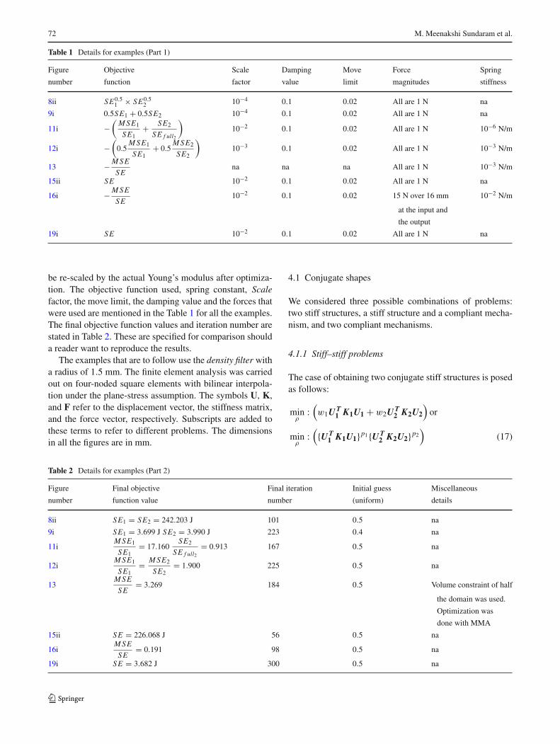
be re-scaled by the actual Young’s modulus after optimiza-tion. The objective function used, spring constant, Scalefactor, the move limit, the damping value and the forces thatwere used are mentioned in the Table 1 for all the examples.The final objective function values and iteration number arestated in Table 2. These are specified for comparison shoulda reader want to reproduce the results.
The examples that are to follow use the density filter witha radius of 1.5 mm. The finite element analysis was carriedout on four-noded square elements with bilinear interpola-tion under the plane-stress assumption. The symbols U, K,and F refer to the displacement vector, the stiffness matrix,and the force vector, respectively. Subscripts are added tothese terms to refer to different problems. The dimensionsin all the figures are in mm.
4.1 Conjugate shapes
We considered three possible combinations of problems:two stiff structures, a stiff structure and a compliant mecha-nism, and two compliant mechanisms.
4.1.1 Stiff–stiff problems
The case of obtaining two conjugate stiff structures is posedas follows:
minρ
:(w1U T
1 K1U1 + w2U T2 K2U2
)or
minρ
:({U T
1 K1U1}p1{U T2 K2U2}p2
)(17)
Table 2 Details for examples (Part 2)
Figure Final objective Final iteration Initial guess Miscellaneous
number function value number (uniform) details
8ii SE1 = SE2 = 242.203 J 101 0.5 na
9i SE1 = 3.699 J SE2 = 3.990 J 223 0.4 na
11iM SE1
SE1= 17.160
SE2
SE f ull2= 0.913 167 0.5 na
12iM SE1
SE1= M SE2
SE2= 1.900 225 0.5 na
13M SE
SE= 3.269 184 0.5 Volume constraint of half
the domain was used.
Optimization was
done with MMA
15ii SE = 226.068 J 56 0.5 na
16iM SE
SE= 0.191 98 0.5 na
19i SE = 3.682 J 300 0.5 na
Conjugate, conjoined shapes and tilings 73
subject to
K1U1 = F1 on ρ�
K2U2 = F2 on ρc�
0 ≤ ρi ≤ 1 f or i = 1...Ne
The nature of the stiff structure problem is such that theobjective is ‘material-hungry’, i.e., it will take as muchmaterial as possible to lower the strain energy. So, thetwo problems compete for material and a compromise isachieved between the two problems. Three examples arepresented to illustrate different features of the conjugatestiff-stiff structures.
In the example shown in Fig. 8, optimization was donewith the multiplicative form of the objective. In such prob-lems with isometric boundary conditions, the final structurefor both the problems must not differ. This is an importantverification that must be carried out during the implementa-tion. In fact, this example revealed the asymmetry inducedby the original sensitivity filter, as stated in Section 3.1.
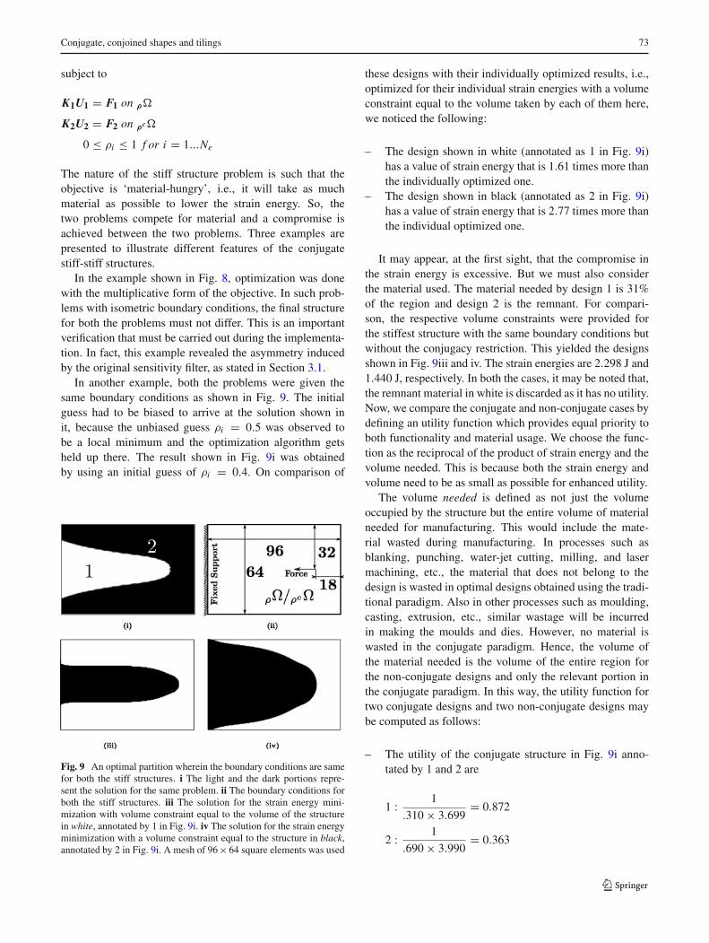
In another example, both the problems were given thesame boundary conditions as shown in Fig. 9. The initialguess had to be biased to arrive at the solution shown init, because the unbiased guess ρi = 0.5 was observed tobe a local minimum and the optimization algorithm getsheld up there. The result shown in Fig. 9i was obtainedby using an initial guess of ρi = 0.4. On comparison of
Fig. 9 An optimal partition wherein the boundary conditions are samefor both the stiff structures. i The light and the dark portions repre-sent the solution for the same problem. ii The boundary conditions forboth the stiff structures. iii The solution for the strain energy mini-mization with volume constraint equal to the volume of the structurein white, annotated by 1 in Fig. 9i. iv The solution for the strain energyminimization with a volume constraint equal to the structure in black,annotated by 2 in Fig. 9i. A mesh of 96 × 64 square elements was used
these designs with their individually optimized results, i.e.,optimized for their individual strain energies with a volumeconstraint equal to the volume taken by each of them here,we noticed the following:
– The design shown in white (annotated as 1 in Fig. 9i)has a value of strain energy that is 1.61 times more thanthe individually optimized one.
– The design shown in black (annotated as 2 in Fig. 9i)has a value of strain energy that is 2.77 times more thanthe individual optimized one.
It may appear, at the first sight, that the compromise inthe strain energy is excessive. But we must also considerthe material used. The material needed by design 1 is 31%of the region and design 2 is the remnant. For compari-son, the respective volume constraints were provided forthe stiffest structure with the same boundary conditions butwithout the conjugacy restriction. This yielded the designsshown in Fig. 9iii and iv. The strain energies are 2.298 J and1.440 J, respectively. In both the cases, it may be noted that,the remnant material in white is discarded as it has no utility.Now, we compare the conjugate and non-conjugate cases bydefining an utility function which provides equal priority toboth functionality and material usage. We choose the func-tion as the reciprocal of the product of strain energy and thevolume needed. This is because both the strain energy andvolume need to be as small as possible for enhanced utility.
The volume needed is defined as not just the volumeoccupied by the structure but the entire volume of materialneeded for manufacturing. This would include the mate-rial wasted during manufacturing. In processes such asblanking, punching, water-jet cutting, milling, and lasermachining, etc., the material that does not belong to thedesign is wasted in optimal designs obtained using the tradi-tional paradigm. Also in other processes such as moulding,casting, extrusion, etc., similar wastage will be incurredin making the moulds and dies. However, no material iswasted in the conjugate paradigm. Hence, the volume ofthe material needed is the volume of the entire region forthe non-conjugate designs and only the relevant portion inthe conjugate paradigm. In this way, the utility function fortwo conjugate designs and two non-conjugate designs maybe computed as follows:
– The utility of the conjugate structure in Fig. 9i anno-tated by 1 and 2 are
1 : 1
.310 × 3.699= 0.872
2 : 1
.690 × 3.990= 0.363

74 M. Meenakshi Sundaram et al.
– The total utility of both the conjugate structures is
0.872 + .363 = 1.235
– The utility of the non-conjugate structure in Fig. 9iii
1
1 × 2.298= 0.435
– The same in Fig. 9iv is
1
1 × 1.440= 0.694
Thus, we can see that the utility of the two conjugate struc-tures, 1.24, is better than the individually optimised ones.In the case with the lower volume the utility is 2.84 timesgreater and in the other case it is about 1.78 times greater.
There is also a caveat in this method: a conjugate designsolution may not always exist. In stiff structures, the fixedsupports and the points of application of the force have tobe connected. In the example shown in Fig. 10, there isno way to connect the two without having an intersectionbetween them. We can see that the solutions are formedthrough one-node connections or the checker-board pat-terns. On increasing the filter radius, we noticed that theoptimization process stays put at a grey solution.The resultwith the checker-board is shown in Fig. 10. This indicatesthat such cases do not have practicable solutions since thereare no non-intersecting paths between the loaded and fixedboundaries of the two problems.
4.1.2 Compliant–stiff problems
The case of a compliant mechanism conjugately com-bined with a stiff structure is studied using the followingformulation.
maxρ
:(
w1M SE1
SE1+ w2
SE f ull2
SE2
)or
maxρ
:(
M SE1
SE1× SE f ull2
SE2
)(18)
subject to
K1U1 = F1
K1Ud1 = Fd1 on ρ�
K2U2 = F2 on ρc�
0 ≤ ρi ≤ 1 i = 1...Ne
where
M SE1 = U Td1
K1U1
SEi = U Ti Ki Ui
SE f ull2 = Strain Energy when the entire region
is given for the problem
The term Fd refers to a unit load at the output point ofthe mechanism in the desired direction and Ud refers to theresulting displacement under its action. The objective func-tion for the stiff structure is formulated as the reciprocalof strain energy as we wanted both the objective functionsto be maximized. A normalization term called SE f ull2 wasmultiplied to this reciprocal of the strain energy to scale theproblem suitably. This term can be computed as the strainenergy when the entire region is provided for the analysisand it is the least strain energy that can be achieved. Further-more, this is just a constant that can be easily pre-computed.Now these are coupled either in additive or multiplica-tive type combinations. In the latter case suitable integralexponents can also be taken to maintain the sense of theoptimization.
The objective functions in this problem are cooperativemeaning that the compliant mechanism is ‘not material hun-gry’ whereas the stiff structure is ‘material hungry’. It istherefore natural that the stiff structure takes away the mate-rial from the compliant mechanism. The results show thatthe compliant mechanism is ‘emaciated’ and works throughone-node hinges with minimal material around it. The rea-son for this is the loop hole in finite element method and the
Fig. 10 A case where theproblems posed have nopracticable solutions. i Thesolution where the light anddark regions intersect throughchecker-board form ofconnections. ii The boundaryconditions for the light region.iii The boundary conditions forthe dark region. A 32 × 32square element mesh was used

Conjugate, conjoined shapes and tilings 75
design parameterization that causes them to undergo largedeformations with low stresses at the one-node hinges. Thisis well-known and documented in the compliant mecha-nism literature (Yin and Ananthasuresh 2003). Such hingeshardly affect the resulting stiff structure as shown in Fig.11. The mechanism in Fig. 11i is intended to reverse thedirection of the input (i.e., to get a displacement-inverter).Here, equal weights were used for the additive form of thecombined objective function.
Upon increasing the weight on the compliant mechanism,the problem of emaciated connections still persists. Thesame behaviour was observed when the combined objectivewas taken as the product of the individual objectives.
4.1.3 Compliant–compliant problem
Since a compliant mechanism problem is generally ‘notmaterial hungry’, it is interesting to see how the material isdistributed between two compliant mechanisms. We studythis using the following formulation.
maxρ
: w1M SE1
SE1+ w2
M SE2
SE2(19)
subject to
K1U1 = F1
K1Ud1 = Fd1 on ρ�
K2U2 = F2
K2Ud2 = Fd2 on ρc�
0 ≤ ρi ≤ 1 i = 1...Ne
where
M SEi = U Tdi
Ki Ui
SEi = U Ti Ki Ui
As noted in the previous discussion, optimization gives riseto one-node hinges in the resulting compliant mechanisms.An example is shown in Fig. 12 where isometric boundaryconditions exist for both the problems. Here, the intentionis to achieve two displacement-inverting mechanisms. Thesolution has vestigial portions for the purpose of creatingfeatures in its conjugate part as can be seen from the anno-tation in Fig. 12i. This is a consequence of the constraintimposed by the parameterization. This can be noticed inmost of the examples.
Fig. 11 The optimal partition for a stiff structure and a compli-ant mechanism to illustrate the co-operative nature of the linear-combination. i The light shade is for a displacement–inverter mech-anism and the dark shade is for a stiff structure. The result indicatesthe emaciation of the one-node hinges through which the compliant
mechanism derives its functionality. ii The boundary conditions for thedisplacement inverter. iii The boundary conditions for the stiff struc-ture. A 64 × 64 square elements mesh was used for half the domain,with roller supports at one end to impose symmetry. iv The deformedmesh for the compliant mechanism
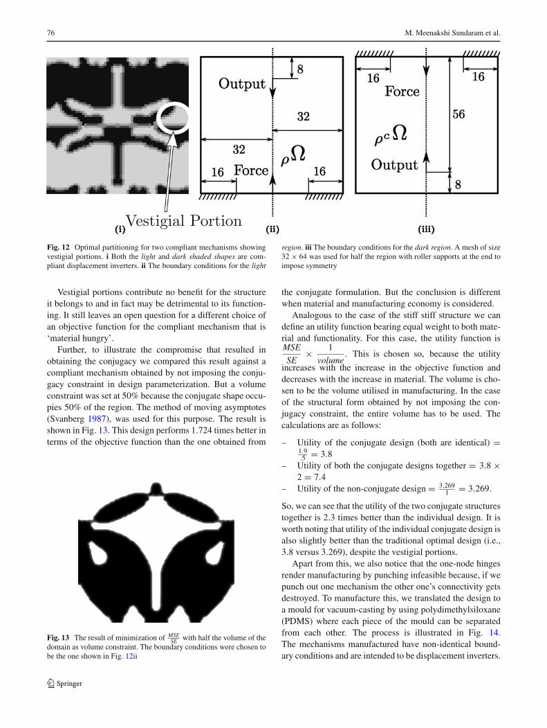
76 M. Meenakshi Sundaram et al.
Fig. 12 Optimal partitioning for two compliant mechanisms showingvestigial portions. i Both the light and dark shaded shapes are com-pliant displacement inverters. ii The boundary conditions for the light
region. iii The boundary conditions for the dark region. A mesh of size32 × 64 was used for half the region with roller supports at the end toimpose symmetry
Vestigial portions contribute no benefit for the structureit belongs to and in fact may be detrimental to its function-ing. It still leaves an open question for a different choice ofan objective function for the compliant mechanism that is‘material hungry’.
Further, to illustrate the compromise that resulted inobtaining the conjugacy we compared this result against acompliant mechanism obtained by not imposing the conju-gacy constraint in design parameterization. But a volumeconstraint was set at 50% because the conjugate shape occu-pies 50% of the region. The method of moving asymptotes(Svanberg 1987), was used for this purpose. The result isshown in Fig. 13. This design performs 1.724 times better interms of the objective function than the one obtained from
Fig. 13 The result of minimization of MSESE with half the volume of the
domain as volume constraint. The boundary conditions were chosen tobe the one shown in Fig. 12ii
the conjugate formulation. But the conclusion is differentwhen material and manufacturing economy is considered.
Analogous to the case of the stiff stiff structure we candefine an utility function bearing equal weight to both mate-rial and functionality. For this case, the utility function isMSE
SE× 1
volume. This is chosen so, because the utility
increases with the increase in the objective function anddecreases with the increase in material. The volume is cho-sen to be the volume utilised in manufacturing. In the caseof the structural form obtained by not imposing the con-jugacy constraint, the entire volume has to be used. Thecalculations are as follows:
– Utility of the conjugate design (both are identical) =1.9.5 = 3.8
– Utility of both the conjugate designs together = 3.8 ×2 = 7.4
– Utility of the non-conjugate design = 3.2691 = 3.269.
So, we can see that the utility of the two conjugate structurestogether is 2.3 times better than the individual design. It isworth noting that utility of the individual conjugate design isalso slightly better than the traditional optimal design (i.e.,3.8 versus 3.269), despite the vestigial portions.
Apart from this, we also notice that the one-node hingesrender manufacturing by punching infeasible because, if wepunch out one mechanism the other one’s connectivity getsdestroyed. To manufacture this, we translated the design toa mould for vacuum-casting by using polydimethylsiloxane(PDMS) where each piece of the mould can be separatedfrom each other. The process is illustrated in Fig. 14.The mechanisms manufactured have non-identical bound-ary conditions and are intended to be displacement inverters.
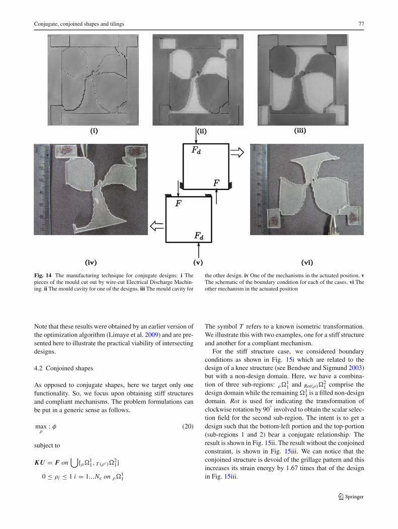
Conjugate, conjoined shapes and tilings 77
Fig. 14 The manufacturing technique for conjugate designs: i Thepieces of the mould cut out by wire-cut Electrical Discharge Machin-ing. ii The mould cavity for one of the designs. iii The mould cavity for
the other design. iv One of the mechanisms in the actuated position. vThe schematic of the boundary condition for each of the cases. vi Theother mechanism in the actuated position
Note that these results were obtained by an earlier version ofthe optimization algorithm (Limaye et al. 2009) and are pre-sented here to illustrate the practical viability of intersectingdesigns.
4.2 Conjoined shapes
As opposed to conjugate shapes, here we target only onefunctionality. So, we focus upon obtaining stiff structuresand compliant mechanisms. The problem formulations canbe put in a generic sense as follows.
maxρ
: φ (20)
subject to
K U = F on⋃
{ρ�11, T (ρc)�
21}
0 ≤ ρi ≤ 1 i = 1...Ne on ρ�11
The symbol T refers to a known isometric transformation.We illustrate this with two examples, one for a stiff structureand another for a compliant mechanism.
For the stiff structure case, we considered boundaryconditions as shown in Fig. 15i which are related to thedesign of a knee structure (see Bendsøe and Sigmund 2003)but with a non-design domain. Here, we have a combina-tion of three sub-regions: ρ�1
1 and Rot(ρ)�21 comprise the
design domain while the remaining �13 is a filled non-design
domain. Rot is used for indicating the transformation ofclockwise rotation by 90
◦involved to obtain the scalar selec-
tion field for the second sub-region. The intent is to get adesign such that the bottom-left portion and the top-portion(sub-regions 1 and 2) bear a conjugate relationship. Theresult is shown in Fig. 15ii. The result without the conjoinedconstraint, is shown in Fig. 15iii. We can notice that theconjoined structure is devoid of the grillage pattern and thisincreases its strain energy by 1.67 times that of the designin Fig. 15iii.
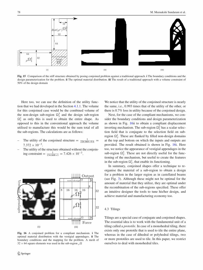
78 M. Meenakshi Sundaram et al.
Fig. 15 Comparison of the stiff structure obtained by posing conjoined problem against a traditional approach. i The boundary conditions and thedesign parameterization for the problem. ii The optimal material distribution. iii The result of a traditional approach with a volume constraint of50% of the design domain
Here too, we can use the definition of the utility func-tion that we had developed in the Section 4.1.1. The volumefor this conjoined case would be the combined volume ofthe non-design sub-region �3
1 and the design sub-region�1
1 as only this is used to obtain the entire shape. Asopposed to this in the conventional approach the volumeutilised to manufacture this would be the sum total of allthe sub-regions. The calculations are as follows:
– The utility of the conjoined structure = 1226.068×0.6 =
7.372 × 10⁻³.– The utility of the structure obtained without the conjoin-
ing constraint = 1134.668×1 = 7.426 × 10⁻³.
Fig. 16 A conjoined problem for a compliant mechanism. i Theoptimal material distribution with the vestigial appendages. ii Theboundary conditions and the mapping for the problem. A mesh of32 × 64 square elements was used in the sub-region ρ�
We notice that the utility of the conjoined structure is nearlythe same, i.e., 0.993 times that of the utility of the other, orthere is 0.7% loss in utility because of the conjoined design.
Next, for the case of the compliant mechanisms, we con-sider the boundary conditions and design parameterizationas shown in Fig. 16ii to obtain a compliant displacementinverting mechanism. The sub-region �2
1 has a scalar selec-tion field that is conjugate to the selection field on sub-region �1
1. These are flanked by filled non-design domainsat the top and bottom on which the inputs and outputs areprovided. The result obtained is shown in Fig. 16i. Heretoo, we notice the appearance of vestigial appendages in thesub-region �2
1. These are not directly useful for the func-tioning of the mechanism, but useful to create the featuresin the sub-region �1
1, that enable its functioning.In summary, conjoined shapes offer a technique to re-
organise the material of a sub-region to obtain a designfor a problem in the larger region as in castellated beams(see Fig. 3). Although these might not be optimal for theamount of material that they utilize, they are optimal underthe recombination of the sub-regions specified. These offeran intuitive designer the tools to tune his/her design, andachieve material and manufacturing economy too.
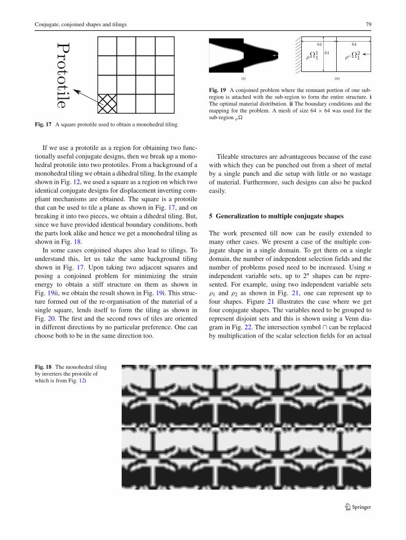
4.3 Tilings
Tilings are a special case of conjugate and conjoined shapes.The essential idea is to work with the fundamental unit of atiling called a prototile. In case of a monohedral tiling, thereexists only one prototile that is used to tile the entire plane,whereas in the case of dihedral or polyhedral tilings, twoor more prototiles are used to tile. In this paper, we restrictourselves to deal with monohedral tiles.
Conjugate, conjoined shapes and tilings 79
Fig. 17 A square prototile used to obtain a monohedral tiling
If we use a prototile as a region for obtaining two func-tionally useful conjugate designs, then we break up a mono-hedral prototile into two prototiles. From a background of amonohedral tiling we obtain a dihedral tiling. In the exampleshown in Fig. 12, we used a square as a region on which twoidentical conjugate designs for displacement inverting com-pliant mechanisms are obtained. The square is a prototilethat can be used to tile a plane as shown in Fig. 17, and onbreaking it into two pieces, we obtain a dihedral tiling. But,since we have provided identical boundary conditions, boththe parts look alike and hence we get a monohedral tiling asshown in Fig. 18.
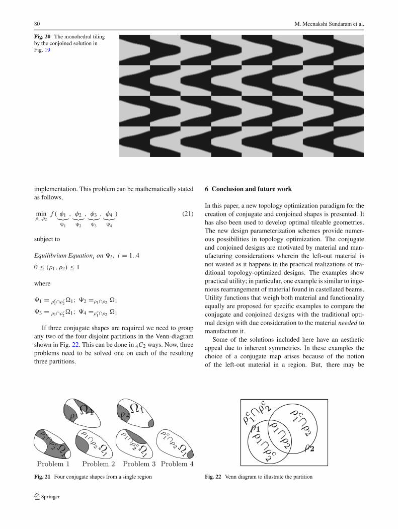
In some cases conjoined shapes also lead to tilings. Tounderstand this, let us take the same background tilingshown in Fig. 17. Upon taking two adjacent squares andposing a conjoined problem for minimizing the strainenergy to obtain a stiff structure on them as shown inFig. 19ii, we obtain the result shown in Fig. 19i. This struc-ture formed out of the re-organisation of the material of asingle square, lends itself to form the tiling as shown inFig. 20. The first and the second rows of tiles are orientedin different directions by no particular preference. One canchoose both to be in the same direction too.
Fig. 19 A conjoined problem where the remnant portion of one sub-region is attached with the sub-region to form the entire structure. iThe optimal material distribution. ii The boundary conditions and themapping for the problem. A mesh of size 64 × 64 was used for thesub-region ρ�
Tileable structures are advantageous because of the easewith which they can be punched out from a sheet of metalby a single punch and die setup with little or no wastageof material. Furthermore, such designs can also be packedeasily.
5 Generalization to multiple conjugate shapes
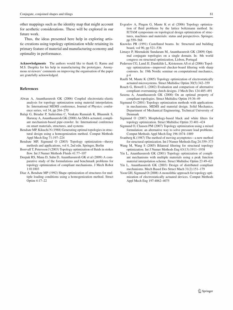
The work presented till now can be easily extended tomany other cases. We present a case of the multiple con-jugate shape in a single domain. To get them on a singledomain, the number of independent selection fields and thenumber of problems posed need to be increased. Using nindependent variable sets, up to 2n shapes can be repre-sented. For example, using two independent variable setsρ1 and ρ2 as shown in Fig. 21, one can represent up tofour shapes. Figure 21 illustrates the case where we getfour conjugate shapes. The variables need to be grouped torepresent disjoint sets and this is shown using a Venn dia-gram in Fig. 22. The intersection symbol ∩ can be replacedby multiplication of the scalar selection fields for an actual
Fig. 18 The monohedral tilingby inverters the prototile ofwhich is from Fig. 12i
80 M. Meenakshi Sundaram et al.
Fig. 20 The monohedral tilingby the conjoined solution inFig. 19
implementation. This problem can be mathematically statedas follows,
minρ1,ρ2
f ( φ1︸︷︷︸�1
, φ2︸︷︷︸�2
, φ3︸︷︷︸�3
, φ4︸︷︷︸�4
) (21)
subject to
Equilibrium Equationi on �i , i = 1..4
0 ≤ (ρ1, ρ2) ≤ 1
where
�1 = ρc1∩ρc
2�1; �2 =ρ1∩ρ2 �1
�3 = ρ1∩ρc2�1; �4 =ρc
1∩ρ2 �1
If three conjugate shapes are required we need to groupany two of the four disjoint partitions in the Venn-diagramshown in Fig. 22. This can be done in 4C2 ways. Now, threeproblems need to be solved one on each of the resultingthree partitions.
Fig. 21 Four conjugate shapes from a single region
6 Conclusion and future work
In this paper, a new topology optimization paradigm for thecreation of conjugate and conjoined shapes is presented. Ithas also been used to develop optimal tileable geometries.The new design parameterization schemes provide numer-ous possibilities in topology optimization. The conjugateand conjoined designs are motivated by material and man-ufacturing considerations wherein the left-out material isnot wasted as it happens in the practical realizations of tra-ditional topology-optimized designs. The examples showpractical utility; in particular, one example is similar to inge-nious rearrangement of material found in castellated beams.Utility functions that weigh both material and functionalityequally are proposed for specific examples to compare theconjugate and conjoined designs with the traditional opti-mal design with due consideration to the material needed tomanufacture it.
Some of the solutions included here have an aestheticappeal due to inherent symmetries. In these examples thechoice of a conjugate map arises because of the notionof the left-out material in a region. But, there may be
Fig. 22 Venn diagram to illustrate the partition
Conjugate, conjoined shapes and tilings 81
other mappings such as the identity map that might accountfor aesthetic considerations. These will be explored in ourfuture work.
Thus, the ideas presented here help in exploring artis-tic creations using topology optimization while retaining itsprimary feature of material and manufacturing economy andoptimality in performance.
Acknowledgments The authors would like to thank G. Ramu andM.S. Deepika for his help in manufacturing the prototypes. Anony-mous reviewers’ comments on improving the organisation of the paperare gratefully acknowledged.
References
Alwan A, Ananthasuresh GK (2006) Coupled electrostatic-elasticanalysis for topology optimization using material interpolation.In: International MEMS conference, Journal of Physics: confer-ence series, vol 34, pp 264–270
Balaji G, Biradar P, Saikrishna C, Venkata Ramaiah K, Bhaumik S,Haruray A, Ananthasuresh GK (2008) An SMA-actuated, compli-ant mechanism-based pipe-crawler. In: International conferenceon smart materials, structures, and systems
Bendsøe MP, Kikuchi N (1988) Generating optimal topologies in struc-tural design using a homogenization method. Comput MethodsAppl Mech Eng 71:197–224
Bendsøe MP, Sigmund O (2003) Topology optimization—theorymethods and applications, vol 4, 2nd edn. Springer, Berlin
Borrvall T, Petersson J (2003) Topology optimization of fluids in stokesflow. Int J Numer Methods Fluids 41:77–107
Deepak RS, Mana D, Sahu D, Ananthasuresh GK et al (2009) A com-parative study of the formulations and benchmark problems fortopology optimization of compliant mechanisms. J Mech Robot1:011003
Diaz A, Bendsøe MP (1992) Shape optimization of structures for mul-tiple loading conditions using a homogenization method. StructOptim 4:17–22
Evgrafov A, Pingen G, Maute K et al (2006) Topology optimiza-tion of fluid problems by the lattice boltzmann method. In:IUTAM symposium on topological design optimization of struc-tures, machines and materials: status and perspectives. Springer,pp 559–568
Knowles PR (1991) Castellated beams. In: Structural and buildingboard, vol 90, pp 521–536
Limaye P, Meenakshi Sundaram M, Ananthasuresh GK (2009) Opti-mal conjugate topologies on a single domain. In: 8th worldcongress on structural optimization, Lisbon, Portugal
Pedersen CG, Lund JJ, Damkilde L, Kristensen AS et al (2006) Topol-ogy optimization—improved checker-board filtering with sharpcontours. In: 19th Nordic seminar on computational mechanics,p 4
Raulli M, Maute K (2005) Topology optimization of electrostaticallyactuated microsystems. Struct Multidisc Optim 30(5):342–359
Roach G, Howell L (2002) Evaluation and comparison of alternativecompliant overrunning clutch designs. J Mech Des 124:485–491
Saxena A, Ananthasuresh GK (2000) On an optimal property ofcompliant topologies. Struct Multidisc Optim 19:36–49
Sigmund O (2001) Topology optimization methods with applicationsin mechanisms, MEMS and material design. Solid Mechanics,Department of Mechanical Engineering, Technical University ofDenmark
Sigmund O (2007) Morphology-based black and white filters fortopology optimization. Struct Multidisc Optim 33:401–424
Sigmund O, Clausen PM (2007) Topology optimization using a mixedformulation: an alternative way to solve pressure load problems.Comput Methods Appl Mech Eng 196:1874–1889
Svanberg K (1987) The method of moving asymptotes—a new methodfor structural optimization. Int J Numer Methods Eng 24:359–373
Wang M, Wang S (2005) Bilateral filtering for structural topologyoptimization. Int J Numer Methods Eng 63(13):1911–1938
Yin L, Ananthasuresh GK (2001) Topology optimization of compli-ant mechanisms with multiple materials using a peak functionmaterial interpolation scheme. Struct Multidisc Optim 23:49–62
Yin L, Ananthasuresh GK (2003) Design of distributed compliantmechanisms. Mech Based Des Struct Mach 31(2):151–179
Yoon GH, Sigmund O (2008) A monolithic approach for topology opti-mization of electrostatically actuated devices. Comput MethodsAppl Mech Eng 197:4062–4075
Related Documents