Design and implementation of an experimental platform for … · 2016-01-07 · Design and implementation of an experimental platform for performance analysis in wireless ... node

Design and implementation of an experimental platform for performance analysis in wireless

sensor networks

ZHEJUN FENG

Master of Science Thesis in Design and Implementation of ICT Products and Systems, KTH

Supervisor: Huimin She Examiner: Associate Prof. Zhonghai Lu

TRITA-ICT-EX-2011:293

ii

Abstract Analysis of transmission delay and throughput in wireless sensor networks (WSNs) is essential for the deployment of WSNs in real applications. Although researchers have already done a lot of theoretic analysis on transmission delay and throughput in WSNs, very few of them gave the real sensor test results. In this master thesis, an experimental platform for wireless sensor networks has been designed and implemented. The purpose of building this platform is to find out the systems and environment factors that have impacts on the transmission delay and throughput of single hop and multi-hop wireless sensor networks. With this platform, we can combine the theory analysis with real field tests and give more reliable analysis on the performance analysis problem. The platform is based on one of the most popular operating system for sensor networks –Contiki OS and the Maxfor CM 5000 sensor motes. On this experimental platform, several groups of simulation tests and field tests in single hop, multi-hop and multi-path sensor networks have been implemented. All of these tests are divided into several groups in order to test different system and environment conditions that impact the transmission delay and throughput. Through the tests, a large amount of information and results about the transmission delay and throughput of the wireless sensor networks has been obtained. To achieve the visualized result and help the analysis, the figures of transmission period time for every type of tests are drawn using Matlab. The results of simulation tests and field tests are compared. We found that the program used in COOJA simulator can be easily transplanted to the real sensor nodes. It is also figured out which test condition would have the effect on the transmission delay and throughput. Moreover, the throughput values of the wireless sensor networks under different conditions are given in the paper.

iii

Acknowledgement I am so glad that I can finish my thesis project under the supervisor Huimin She. He has given me a lot of help during my thesis. He is not only my thesis supervisor but also like a friend to encourage me to perform better in the thesis project. I am very thankful to his valuable suggestions and introductions. Thanks also to examiner Zhonghai Lu who reviewed my work and gave very useful feedback to the report. Thanks very much to my parents, my girlfriend and all my friends. Thanks for their support and help. That is how I can study and keep moving forward. .

iv

Content Abstract ......................................................................................................................... ii Acknowledgement ...................................................................................................... iii 1 Introduction ............................................................................................................... 1

1.1 Problem statement and motivation ...................................................................... 1 1.2 Work phase and Methodology ............................................................................. 2 1.3 Thesis structure ..................................................................................................... 3

2 Background ............................................................................................................... 4 2.1 Wireless sensor networks ...................................................................................... 4 2.2 Contiki operating system ...................................................................................... 6 2.3 CM5000 Mote ........................................................................................................ 8 2.4 IEEE 802.15.4 ........................................................................................................ 9 2.5 X-MAC and NULL-MAC protocols .................................................................. 10

3 Simulation and Implementation ............................................................................ 12 3.1 Theoretic calculation of delay and throughput ................................................ 12 3.2 Simulation in COOJA ......................................................................................... 15

3.2.1 Different simulation conditions ..................................................................... 16 3.2.2 Design of the application program ............................................................... 18 3.2.3 Simulation result in different conditions ...................................................... 22

3.3 Field Test .............................................................................................................. 37 4 Comparison and Conclusion of test ...................................................................... 52

4.1 Comparison of experiment data .............................................................................. 52 4.2 Conclusions of the test .............................................................................................. 57

5 Result and future work ........................................................................................... 59 5.1 Result .......................................................................................................................... 59 5.2 Future Work .............................................................................................................. 59

Reference .................................................................................................................... 60 Appendix A ................................................................................................................. 62 Appendix B ................................................................................................................. 64

1

Chapter 1

Introduction

During the last ten years, wireless sensor networks (WSNs) have attracted increasing attention from not only research institute but also real industrial. The technology of wireless sensor networks develops very fast thanks to the advancement of digital electronic technology and wireless communication technology. WSNs are composed of a large number of sensor nodes that are deployed spatially in indoor or outdoor environment. These sensor nodes can be used to detect the surround conditions such as temperature, light, sound, humidity and so on. It means that there are numerous application areas for WSNs, for example, military surveillance, disaster detection, industrial automation and smart home etc.

The wireless sensor networks consist of sensor nodes from a few to several hundreds. Each node is connected to another sensor node (sometimes several nodes). A typical wireless sensor node is composed of 4 parts: sensors, a radio transceiver, a microprocessor unit and an energy source. All the wireless sensor nodes use the radio chip to transmit and receive the radio signals.

There are many kinds of topology of wireless networks like star network, multi-hop mesh network and cluster tree network. Customers can choose the specific topology of network according to its application area.

The cost of wireless sensor networks will change dramatically depending on its function and application area. But in most of situation, real industrial companies will try to minimize the cost of sensor node because of the large quantity of the nodes and the simplicity of the task. At the same time, the constraint of size and cost of sensor node will also limit its memory capacity, processor speed and transmission bandwidth. So how to choose a suitable sensor node for the application is very important.

1.1 Problem statement and motivation Because of the limitation of energy consumption and transmission bandwidth, wireless sensor node can not transmit data as fast as Bluetooth or Wi-Fi. They are utilized in totally different applications. The focus of WSNs is low cost, very low power, short range and small size. To achieve these aims, a lot of research work has been performed in designing a low power MAC protocols. X-MAC is one of the asynchronous duty-cycled MAC protocols for achieving low power consumption in WSNs. It can help to significantly reduce energy usage at both transmitter and receiver and reduce per-hop latency in multi-hop network.

In this master thesis, an experiment platform based on the real sensor nodes was designed and implemented to test the transmission period time and throughput of wireless sensor networks. CM5000 mote was chosen as the real sensor node and Contiki was chosen as the operating system for the sensor node.

2

The CM5000 mote [2] is an IEEE802.15.4 compliant wireless sensor node and is ContikiOS compatible. It has integrated all the necessary functionalities in one hardware module: three sensors, processor unit, power supplier and wireless communication transceiver. So it is especially suitable as a research platform for developers. Contiki is a pioneering, very concise, highly influential open source operating system for wireless sensor networks. It includes the COOJA Simulator which is a cross level simulation tool for the application development. We can use the function of COOJA to precisely calculate the latency and transmission period time of data. This advantage is one of the reasons that I choose Contiki as the operating system of the sensor nodes.

After finishing preparing all these essential components for the experimental platform, the next step is to implement simulation test and field test of data transmission between sender and receiver. In this thesis project, many transmission models are used to test the wireless sensor networks and calculate the throughput with various internal and external conditions. The purpose of this thesis is to compare the simulation test result and real field result and find the effective conditions.

The motivation of my thesis project is coming from the concept that transmission period and throughput estimate are very important for many WSNs applications such as battle surveillance which will generate a large amount of data in a short time. If the transmission rate and throughput of network is not fast enough, it will bring serious problem for the user. What’s more, while there are already some theoretic studies for X-MAC protocol, there are still few practical experimental platforms to test the throughput of X-MAC based on the real sensor nodes and operating system. Moreover, what kind of conditions will affect the transmission period and throughput of wireless sensor networks is also the question that I concerned.

1.2 Work phase and Methodology This master thesis project can be divided into these following work phases: ��Literature study ��Platform design ��System implementation ��Test of data ��Analysis of result In the beginning of this thesis, the fundamental concept and knowledge about wireless sensor networks, X-MAC protocols and Contiki operating system will be studied. Without this knowledge, it is almost impossible to choose the suitable components and build the test platform. There are also some previous articles introducing the calculation of energy and latency of X-MAC in WSNs. Studying and understanding all these literature can help me to better analyze the test result.

This thesis is also an experimental project. It includes platform implementation as well as measurement of transmission period and throughput of WSNs. Contiki operating system is an

3

open source software for the wireless sensor networks which is developed in recent years by the Swedish Institute of Computer Science (SICS) [3]. People are authorized to download this system for free from their website. Meanwhile, five CM5000 motes were bought as the real sensor nodes which are compatible with Contiki OS. After finishing these steps, three network models are designed to transmit data packet. They are single hop, two hop and multipath networks. The above work is accomplished in the first 2 months.

The next phase of the thesis project is to make use of platform to test the throughput of wireless sensor networks. For the sake of getting the accuracy transmission period time of data packet, the transmission process will repeat one thousand times in every test. Then the MATLAB software is used to calculate the average transmission period time and draw it into the figures.

The last step is to analyze the difference between theoretic result, simulation result and field test result according to the visualized diagrams and experiment data and get the conclusion. That is the finial purpose that we want to realize.

1.3 Thesis structure This thesis report is composed of five parts: Introduction, Background, Simulation and implementation, Comparison and conclusion, Result and future work. The Background Chapter will describe the fundamental theory of wireless sensor networks, MAC layer protocols and Contiki operating system. It can help the readers to have a better understanding of techniques used in the experiment platform. The simulation and implementation chapter will give an explanation how the data transmission is simulated in COOJA simulator and the test is implemented in real sensor nodes. The details of the experiment will also be introduced in this chapter. In the next chapter, we will analyze the data that we obtained from many experiment tests and deduce some conclusions about transmission period time and throughput according to the figures and data. The following chapter is about the result and future work. The final result of this thesis and discussion about the future work that I should have will be given in this chapter.

4

Chapter 2

Background

Wireless sensor networks consist of many sensor nodes which can transmit data to each other. This network can be used to monitor various conditions and send back the information to the central controller. IEEE 802.15.4 is a standard used in these networks physical and MAC layers. There are two MAC protocols: X-MAC and Null-MAC which are used in this platform test. The CM5000 mote was chosen as the wireless sensor node which is IEEE 802.15.4 compliant. The operating system running in the sensor node is the Contiki OS [3].

In this chapter, the basic knowledge about the wireless sensor networks will be introduced firstly. Then every part of the wireless sensor networks including the sensor nodes, operating system and physical and MAC layers will be explained.

2.1 Wireless sensor networks

Sensor node is the core component of the wireless sensor networks. With the advance of digital electronic circuit, wireless communication technology and low power processor, it has been possible for the researchers to develop a low power, low cost, multifunction sensor node. A single sensor node is composed of a microcontroller, a radio transceiver, a power supply module and several sensors.

As the core of the sensor node, we would like to choose a low power consumption CPU as the microcontroller which has sufficient computation and processing capacity. Most of the data achieved from the sensors will be processed firstly in the microcontroller, and then transmitted to other nodes. The radio transceiver module can use the internal antenna or connect to an external antenna depending on the different applications. Power supply module has attracted a lot of interest from the developers. Because after the sensor node is deployed in the environment, it is difficult for people to charge the battery or replace with new battery. Most of the time, the lifetime of battery decides the lifetime of sensor node.

The most important software which is running in sensor nodes is the operating system. Embedded operating system is much less complex than the general-purpose system. TinyOS [14] is the first operating system specifically designed for wireless sensor networks. But in my thesis project, the Contiki OS was chosen as the operating system for the sensor nodes which used C language as the programming language. It has many advantages compared with other sensor network operating systems. It includes an embedded simulation tool: COOJA, which can compile and simulate the application software conveniently and fast.

There are many different types of sensors that have been developed in recent years. They can be used to monitor a wide variety of conditions. Some types of sensor were listed as follows:

5

�Temperature �Light condition �Humidity �Movement �Pressure �Gravity

According to the specific application, we can integrate the particular sensors we want on the sensor node. A few or a large amount of sensor nodes collaborating with other nodes can form a sensor network. In the network, the data is transmitted with wireless transceiver. The sensor network supports 3 types of topologies: Star Topologies, Peer-to-peer Topology and Cluster-tree Topology [15]. Applications that benefit from the Star topology include home automation, personal computer peripherals, toys and games. A Peer-to-peer network can be ad hoc, self-organizing and self-healing which is suitable for the applications such as industrial control and monitoring, asset and inventory tracking. The advantage of Cluster-tree topology is the increased coverage area.

Star

Mesh

Cluster Tree

Figure 1 The topology modes of wireless sensor networks

Figure1 shows three different topology modes of wireless sensor networks. Each mode

has its special application area. The sensor networks are different with other networks. It includes the following characteristics:

�Mobility of nodes �Dynamic network topology �Large scale of deployment �Ease of use

6

�Unattended operation

The wireless sensor networks also can be connected to the Internet through a gateway node to form the Internet of things [10]. The modern networks are bi-direction which means that it enable the computer to control the activity of sensor nodes as well.

Figure 2 Wireless sensor networks connecting with Internet

Due to the advantage of wireless sensor networks, it can be applied in many new situations. We categorize the applications of WSNs into several classes. For example it can be applied in military surveillance, environment detection, heath care, smart home and other commercial areas.

2.2Contiki operating system

Contiki is an open source, highly portable, multi-tasking operating system developed for use in memory-efficient networked embedded systems and wireless sensor networks [5]. It is designed for the microcontroller which only has small amount of memory. Although it provides both multitasking and a built-in TCP-IP stack [8], a typical Contiki configuration is just 2 kilobytes of RAM and 40 kilobytes of ROM. The basic kernel and most of the core functions were developed by Adam Dunkels at the Swedish Institute of Computer Science. The advantages of the Contiki operating system will be introduced in the following passages.

��Various Hardware platform

Contiki runs on a variety of platforms ranging from embedded microcontrollers such as the TI

Sensor Node Gateway Sensor Node

7

MSP430, ARM7 and the Atmel AVR to old home computer. In this thesis project, the TI MSP430 was chosen as the microcontroller of the sensor nodes. This chip is famous for the character of super low power consumption.

��Low-power radio communication

Contiki operating system provides both full IP network and low power radio communication mechanism with three communication stacks. They are Rime [6], uIP and uIP6. uIP [7] is a minimal fully RFC compliant TCP/IPv4 stack while uIP6 is the world’s smallest fully RFC compliant TCP/IPv6. But in this thesis, the sensor network will not be connected to Internet. So there is no need to use the IP network. Rime is a lightweight layered low-power radio networking stack that provides basic communication primitives and simple abstractions to more complex ones.

�Power efficiency

Since the power consumption of sensor node decides the lifetime of sensor network, lots of researchers are trying to theoretically analyze and test the power consumption of each node. Contiki provides a useful software-based power profiling mechanism that can keep track of the energy consumption of each sensor node. It estimates the energy consumption by measuring the duration of each component in various modes such as low-power mode and transmitting mode. This power profiling mechanism can be used as a research tool for experimental evaluation of sensor network protocols.

�The coffee file system

Contiki provides a Coffee flash-based file system to store data inside the sensor network. It is quite convenient for users to read and write data in flash. In this thesis, the Coffee file system was used to store a large amount of transmission period time data and write them into a text file. No need to print out to console all the time.

�Programming model

Contiki consists of an event-driven kernel, on top of which application programs can be dynamically loaded at run time. Compared with multithreaded kernel, event-driven requires less memory and only need one stack. The processes can be invoked whenever some events happen. On top of the event-driven kernel, they also developed a new process called protothreads [7] which combined the character of events and threads process. It has sequential flow of control without explicit state machine, just like threads process. But it has single stack, just like events process. The whole Contiki system and application programs are written in the C programming language.

�Simulators

Simulator is a very useful tool for the software development in wireless sensor networks. Contiki provides a simulation environment: the COOJA cross-layer network simulator to facilitate software development and debugging. COOJA is a flexible java-based simulator

8

which supports C program language as the software design language by using Java Native Interface (JNI). This approach can make the simulated application run in the real Contiki system and then run on the real sensor node without any modification.

Furthermore, COOJA allows for simultaneous simulations at three different levels, namely the networking level, the operating system level and the machine code instruction level. User can alter parts of the simulation environment without changing any COOJA main code. It means the system can be added new parts such as interfaces, plugins and radio mediums or reconfigured existing parts.

2.3 CM5000 Mote

Figure 3 CM5000 mote

The CM5000 mote is IEEE 802.15.4 compliant wireless sensor node. The mote has the following general characteristics: · �IEEE 802.15.4 WSN platform · �TI MSP430 Processor, CC2420 RF · �TinyOS 2.x & ContikiOS Compatible · �Temperature, Humidity, Light sensors · �User & Reset Buttons · �3xLeds · �USB Interface · �2xAA Battery Holder

The heart of the CM5000 sensor mote is a TI MSP430F1611 microcontroller. This microcontroller belongs to the Texas Instruments MSP430 family of ultralow power

9

microcontrollers. This chip has five low power modes which are optimized to achieve extended battery life in portable applications.

The radio transceiver chip on the board is TI CC2420 [1]. TI CC2420 is a true single-chip 2.4 GHz IEEE 802.15.4 compliant RF transceiver. It is designed for low power and low voltage wireless applications. CC2420 includes a digital direct sequence spread spectrum baseband modem providing a spreading gain of 9 dB and an effective data rate of 250 kbps. The CM5000 has integrated temperature, humidity and light sensors and can be powered either by plugging the USB to a host computer, or by using batteries.

This product is especially suitable not only as a real product to detect the environment, but also as a very useful research platform for developers. Because it has included in the same hardware module all the needed functionalities: sensor readings, processor power and wireless communication potential.

2.4 IEEE 802.15.4 Wireless Personal Area Network (WPAN) is focus on a small space around a person or object that typically extends up to 10m in all direction which is different with Wireless Local Area Network (WLAN). It was created by IEEE 802.15 working group. The characteristic of WPAN is low cost, low power, short range and very small size. Currently, there are three types of WPANs which are different in data rate, battery drain, and quality of service (QoS). The low rate WPAN (IEEE802.15.4/LR-WPAN) [4] is intended to serve a set of industrial, residential and medical applications with very low power consumption. It is also the standard for the wireless sensor networks. IEEE 802.15.4 working group is now detailing the specification of PHY and MAC by offering building blocks for different types of networking.

�� IEEE 802.15.4 PHY

The PHY provides two services for the transmission: the PHY data service and PHY management service interfacing to the physical layer management entity (PLME). The features of the PHY are activation and deactivation of the radio transceiver, energy detection (ED), link quality indication (LQI), channel selection, clear channel assessment (CCA) and transmitting as well as receiving packets across the physical medium.

The standard offers two PHY options based on the two unlicensed RF worldwide frequency band (2.4GHz global, 915 MHz Americas or 868MHz Europe). The data rate is 250kbps at 2.4GHz, 40kbps at 915MHz and 20kbps at 868MHz.

10

PHY (MHz)

Frequency Band (MHz)

Spreading parameters

Chip rate (kchip/s)

modulation Bit rate (kb/s)

Symbol rate (ksymbol/s)

symbols

868/915 868-868.6

300 BPSK 20 20 Binary

902-928

600 BPSK 40 40 Binary

2450 2400-2483 2000 O-QPSK 250 62.5 16-ary orthogonal

Table 2.1 Frequency bands and data rate

�� IEEE 802.15.4 MAC

The medium access control (MAC) enables the transmission of MAC frames through the PHY data service. It provides two services: the MAC data service and the MAC management service interfacing to the MAC sublayer management entity (MLME) service access point (SAP) (MLME-SAP).

The features of MAC sublayer are beacon management, channel access, CTS management, frame validation, acknowledgement delivery, association and disassociation.

2.5 X-MAC and NULL-MAC protocols Energy-efficiency is a fundamental concern in the design of routing and MAC layer protocols for wireless sensor networks (WSNs). One of the most widely used mechanisms for achieving low power consumption in energy constraint WSNs is duty-cycling at the MAC layer. Duty-cycling greatly reduces idle listening, which costs a lot of energy in wireless sensor networks [5]. Idle listening is the spare time that the node is still awake and listening to the medium even though there is no packet being transmitted to the node.

There are mainly two categories of duty-cycling MAC protocols for the wireless sensor networks. One is synchronized protocols, such as S-MAC [16] and T-MAC [17]. Synchronize means that sender and receiver will negotiate a schedule within one frame that regulate when they should be awake and sleep. It can reduce the time and energy wasted in idle listening. But it needs extra space to store the schedule information and complicated mechanism to make sender and receiver synchronize.

Asynchronous duty-cycled MAC protocols, such as B-MAC [12] and X-MAC [13], rely on low power listening (LPL) which is also called preamble sampling. When a sender needs to transmit data, it will transmit a preamble first. When the receiver wakes up and detects the preamble, it will stay awake to prepare receiving the data. Idle listening is reduced in asynchronous protocols because the receiver only wakes for a short time to sample the channel. If there is no data transmitting on the medium, the receiver will turn back to sleep immediately. Asynchronous protocols remove the energy overhead for synchronization, and they are easier to be implemented, as they do not require clock synchronization.

11

X-MAC is an advance approach with low power listening in wireless sensor networks which belongs to the asynchronous duty-cycled MAC protocols. The design goals of the X-MAC protocol are listed as follows:

�Energy-efficiency �Simple, low overhead, distributed implementation �Low latency for data �High throughput for data �Applicability across all types of packetizing

There is a series of mechanisms in X-MAC which are developed by researchers to promise the realization of these goals. As an asynchronous MAC protocol, it does not have to store the schedule information and only keeps awake very short time. It can wake up more often to maintain a low duty cycle. This mechanism can help to reduce latency and make higher throughput. In the X-MAC protocol, it has already embedded the target ID in the preamble to avoid overhearing problem.

One of the disadvantage of LPL is that non-target receiver has to keep awake until the end of the preamble if it samples that a preamble is being sent on the medium. The receiver can not estimate who is the target node of the data, therefore it can not turn back to sleep. This is term as the overhearing problem. In X-MAC, researchers solved this overhearing problem by containing the ID of target node in the preamble. When a node waked up and received a preamble, it read the target node ID which is already included in the preamble packet. If the node is not the intended receiver, the node returned to sleep immediately. If the node is the target receiver, it remains awake for the next data packet.

LPL sends a long preamble to make sure that the receiver has waked up and already received the preamble. But It makes the receiver have to keep awake and wait until the end of entire preamble. Meanwhile other senders also can not transmit data until the channel is clear. In the development of X-MAC, researchers design a solution for this problem. In X-MAC protocol, the sender transmits a series of short preamble packets which are called strobes instead of a long preamble packet. So if the receiver is awake and has received the strobe packet, it can send back an acknowledgement packet immediately during the gap time between two strobes. This mechanism can greatly reduce the multi-hop latency and save the energy unnecessarily in waiting and transmitting.

12

Chapter 3

Simulation and Implementation

In this thesis the transmission period time and throughput of single hop and multi-hop wireless sensor networks was tested based on one of the most popular operating systems for sensor networks – Contiki and the Maxfor CM 5000 sensor motes. But before implementation of this goal, we will firstly do theoretic analysis and simulation in COOJA.

In this chapter, the theoretic calculation method of delay and throughput in wireless sensor networks with X-MAC was introduced. Delay means the transmission latency between sender and receiver. Throughput is the maximum amount of data can be delivered per unit time. After that, we will design the software program and do simulation in ContikiOS embedded simulator COOJA. At last, the field test will be implemented in the real sensor nodes in a single hop and multi-hop sensor networks. Both the simulation and field test will be achieved in many transmitting modes and with different environment conditions.

3.1 Theoretic calculation of delay and throughput

X-MAC is one of the MAC layer protocols that are supported by Contiki operating system. So we will mainly introduce and analyze the theoretic calculation method of delay and throughput under this MAC protocol. Compared with other MAC protocols, its characteristic is the power efficiency, low overhead, low latency and high throughput.

It is also an asynchronous duty cycling MAC protocols. It will turn the radio off and on periodically namely sleep and wake time alternately. During the wake time, the radio switches on and listens for the short preamble. In off time, the radio turn off and save a lot of energy. The duration of sleep and wake period will decide the energy consumption. Users can set sleep and wake parameters in the software to choose a better balance between energy consumption and throughput. The performance of X-MAC is largely determined by this choice for both sender and receivers.

Users need to change the sleep and wake time dynamically in some situations. For example, in a tree topology sensor network, the node close to the terminal node needs to forward much more data packets than those leaves nodes. So we should formulate different sleep schedules for nodes with different traffic load. It means that we can design the software to make the sensor network adapt to traffic load.

13

Long preamble

SendDATA

ACK

RecvData

SendData

RecvData

LPLSender(S)

LPLRecv(R)

X-MACSender(S)

X-MACRecv(R)

time

time

time

time

Extend wait time

R wakes up Listen for queued packets

Short preamble with target address info

Receive early ACK

R wakes up Send early ACK

Time and energy saved

Figure 4 Comparison of the timeline of LPL’s preamble and X-MAC’s short preamble

Low power listening (LPL) is one key mechanism used in asynchronous duty cycling B-MAC [12] protocol. X-MAC has achieved some improvement based on the LPL technology. According to the figure 4, I will explain the specific difference between these two MACs and give the theoretic calculation method.

In LPL MAC, the sender will send a long preamble before it starts transmitting data packet. The target address of the receiver will be included in the data header. When a receiver wakes up, it listens to the medium. If there is a preamble transmitting, it remains awake until the end of the long preamble, and then it receives the target address. If the receiver is not the target node, it turns off the radio and turns back to sleep. Otherwise, it keeps awake and receives the data packet until finishing transmitting. After that, it will still keep the radio turn on and listen for a while to make sure there is no other packet waiting to be received.

In the development of X-MAC, researchers have divided the long preamble to a serial of short preambles. Every preamble includes the target address information. So when the receiver detects the short preamble in the channel, it can determine immediately whether it is the target receiver. If it is the target, it will terminate the sender transmitting the short preamble and send back an Acknowledgement. After the sender got the ACK, it started transmitting data packet. From this figure and analysis, we will find that with the X-MAC, both the sender and receiver can save a lot of transmission period time and energy.

14

Figure5 The Timeline of single hop network in COOJA simulator In order to compare with the theoretic timeline of X-MAC, the timeline figure in the simulation from the COOJA was showed above. In the figure 5, node 1 is the sender and node2 is the receiver. The grey bar means the radio is turned on. From the figure, we can see that the radio is turned on and turned off periodically. This period is determined by the parameter of Channel check rate in the software. Sensor node can only receive the packet when the radio is turned on. The radio on time is very short in order to save the power. The small blue square represents the process of sending packet which can be the preamble or the real data packet. The small green square represents the process of receiving packet. If the receiver node did not get the preamble, the sender will keep sending the short preambles. When the node 2 received the preamble, it would send an ACK to node 1 during the gap time between two preambles. Then the node 1 started sending data packet. From the figure 4 and figure 5, we can see that the theory mechanism of X-MAC fit very well with the practical simulation result.

After analysis of the mechanism of X-MAC, the theoretic calculate equation of latency time was given. The expected delay can be calculated in terms of the duration of the sender and receiver sleep, listen and transmit periods. If S p , Sd and Sal were used to denote the duration of the short preamble time, data transmission time and acknowledgement listening time of sender. R l , sR and R a denote the receiver listening time, sleep time and ACK send time. Then based on the mechanism in Figure 4, the expected latency for the single-hop wireless sensor network can be expressed as follows: Lat= (duration of preamble +ACK listen)*(expected number of iterations required)

+ (duration to send packet)

= ( )

s

1 S S SR SR +R

p al dl p

l

⎛ ⎞⎜ ⎟⎜ ⎟∗ + +⎜ ⎟−⎛ ⎞⎜ ⎟⎜ ⎟⎜ ⎟⎝ ⎠⎝ ⎠

(1)

=( )( )sS S R +R

SR S

p al ld

l p

++

−

15

But all the parameters above need to be restricted in the range of variable value to make

our model reasonable.

{ }sR ,R ,R ,S ,S ,S 0l a p d al > (2)

R Sl p> Preamble reception possible (3)

S Ral a> ACK reception possible (4)

From the above equation, we can deviate the following theorem that when S p andSal are

set to the lowest value, we can get the minimal latency value.

3.2 Simulation in COOJA

Simulator is a very useful tool for the application software development in wireless sensor networks. Before simulator coming up, the code development is very difficult and tedious for users due to the long compilation and debugs time and the transplant problem of the program. With the simulator tool, users can obtain much benefit during the software development phase and large scale test phase.

COOJA is a wireless sensor network simulator designed for the Contiki operating system. It is a flexible java-based simulator which supports using C language to develop application software by Java Native Interface. One of the great advantages of this COOJA simulator is that it can simulate the application software simultaneously in high level algorithm development and low level hard driver development.

The COOJA simulator has great extendibility. Application developer can alter parts of the simulation environment without changing any COOJA main code. It means that the system can be added new parts such as interfaces, plugins and radio mediums or reconfigured existing parts.

With these advantages of COOJA, we can implement variant simulations with different conditions and system settings such as different packet generation rates, different MAC protocols and different network topology.

16

Figure 6 The interface of the COOJA simulator

The interface of COOJA is composed of many plugins. The common used plugins are control panel, radio logger, log listener, timeline and simulation visualizer. The control panel decides the start and pause of the simulation. In the radio logger, it will show the transmission nodes and packet content. It is very helpful for user to analyze the data packet content. In the log listener, developer can use the printf function to output the information from the sensor nodes. The simulation visualizer can give us the visual process of transmission between sender and receiver. We have introduced the timeline before that it is a very useful plugin to help the user analyze the whole process of transmission.

3.2.1 Different simulation conditions

In this thesis, a series of application software programs were designed to simulate the transmission process in wireless sensor networks. During the simulation, there are some key factors in the programs that may have the effect on the transmission period time and throughput of WSNs. These effective factors will be analyzed according to the data obtained from the simulations. 1) First of all, the simulations of data transmission are tested in three network transmission modes. These network transmission modes are used to test the different effective factors.

17

A Single hop (one sender, one receiver) Single hop means that there is only one sender and one receiver. The sender will transmit data to the only one receiver. The receiver should be located in the coverage of sender radio signal. B Two-hop (one sender, one relay node, one receiver) In the two hop network, there are three nodes: sender, relay node and receiver. In this situation, if the sender is too far away from the receiver and the transmitting power is constraint due to the power consumption or other reasons, the sender has to transmit the data to the nearest node namely the relay node firstly. Then the relay node resends the data to the receiver. C Multipath (one sender, more than one relay node, one receiver) The single hop and two hop modes are easy to be understood. The third mode is the multi-path transmission mode. In this mode, there are still only one sender and receiver. But there may be another more than one node that are located between sender and receiver as the relay nodes.

Before the simulation and field test, every sensor nodes has already been assigned a unique node ID. The node ID will be burned into EEPROM and used as the node address in the program. The Node ID is a very important factor to consist of the wireless sensor networks especially in the complicate topologies.

The sender can transmit the data to the target node according to the address information which is contained in the data packet. If the sender can not transmit the data to the receiver directly due to the far distance, it will use the Unicast channel to transmit the data packet to every relay node in case that some of the path is in very bad condition.

The transmission period time is calculated since the data left the sender until it arrived in the receiver. In the simulation test, in order to test if the transmission period time is related with the different relay node, the sender will generate random relay node address. So the data is also be transmitted to the relay node randomly. After the relay node receiving the data from sender, it will resend the data to the target receiver node. Then the receiver node disassembles the data packet and read the relay node address. So the channel conditions of different transmission paths can be analyzed according to the period time. If the receiver can not get the data from one certain relay one, it means that relay node in the path does not work or the test condition is very serious.

SND

RLY

RLY

RLY

RCV

�

Figure 7 Multi-path transmission mode

18

Figure 7 shows the multi-path network mode tested in the experiment. There are three relay

nodes located between sender and receiver. Every relay nodes is in the coverage of the sender’s radio signal. The relay node will not send data to the other relay nodes.

2) The different conditions that have been tested are introduced in the following part. Firstly, the transmission of data packet in WSNs will be simulated with two different packet generation methods in single hop mode.

a. Periodic packet generation rate.

b. Packet generation rate according to Poisson distribution

Periodic generation rate means that the sender generates the data packet and transmits it with a constant frequency in simulation, for example, 1 data packet per second or 1000 data packets per second. Another generation rate is based on Poisson distribution. Poisson distribution means that the interval time between packets is discrete probability distribution. So the data packet generation rate will change all the time in the simulation process.

The programs will also be simulated under two MAC protocols in COOJA: NULL-MAC and X-MAC in order to compare their difference. It is estimated that the transmission period and throughput will change dramatically with different MAC protocols. These programs are also tested in the single hop network.

All of the above simulation conditions can be seen as the system internal conditions. We

can modify the application software to change these conditions. But in the field test, the transmission period and throughput may be also affected by the environment variables such as distance, transmission power of sensor node and interference from other radio source. These environment conditions will also be tested in the field test.

�

3.2.2 Design of the application program

�

COOJA is a network simulator and use MSPsim to simulate the program for the Tmote Sky

nodes. Tmote Sky is a mote platform for the low power, high data rate and high reliable

sensor network applications. CM5000 mote belongs to this platform. COOJA simulator has

already integrated Tmote Sky nodes in the simulation system.

MSPsim is an emulator for MSP430 microcontroller. COOJA has two communication

stacks: Rime stack and IP stack. IP stack is compliant with TCP/IP protocol stack, so it can be

used to connect the node with the Internet. Rime stack is the lightweight protocol stack

consisting of many layers built on each other from basic single-hop broadcast to reliable

multi-hop flooding. In this simulation test, I will use the Rime stack as the commutation stack

for Tmote Sky node.

19

After starting the COOJA simulator, I need to create a new simulation and choose the

Tmote Sky as the node type. Then I need to design the application software program for the

single hop, two hops and multi-path network. The sensor nodes communicate with each other

through the unicast channel. The application program can be mainly divided into two parts.

One is the main process for sending data packet. The other one is the call back function which

will execute automatically after receiving the data packet in the receive node.

In the transmitting process, the sending function was designed. It has a memory buffer so

that the data will be stored in the buffer firstly before sending to the receiver node. In the

function, the value of the target node address is also assigned. If the program is tested in the

multi-path network, the target node address will be generated randomly all the time in the

function.

In the call back function, the receiver will also use the same unicast channel to get the data.

The function is also designed to be able to store the data into the coffee file system and print

out on the screen. So the data can be read again and save in a txt file after finishing the

transmission.

I have drawn these two flow charts and given the explanation in the following parts.

20

End

i<5000

Process Start

Unicast process

Open channel

Set TX power

i=0

Set etimer

Wait for expire of etimer

Copy data, set target address

Send data

i++

No

�

Figure 8 The sending process of unicast communication in the sender

In the beginning of this program, it has to set a channel number for unicast communication

so that both sender and receiver can transmit data in this channel. Then we can set the

transmission power of sender which will decide the coverage range of the radio signal. In

21

order to achieve more precise data about transmission period, the sending process will repeat

1000 times for each simulation.

There are four types of timers in Contiki: timer, etimer, ctimer and rtimer. Etimer is an

active timer which will trigger an event when it expires. Every time, the process needs to wait

for the event from etimer. If the etimer expired, the process can continue to the next step.

Then it will copy the data to the buffer stack and set the address of the target receiver.

Call back function

J++

J=0

If j=1

Transmit time=clock_time()-

Temp

First time receiveTemp=clock_time()

Write transmit time to file

Open the file

Close the file

Receive the data

No

Yes

�

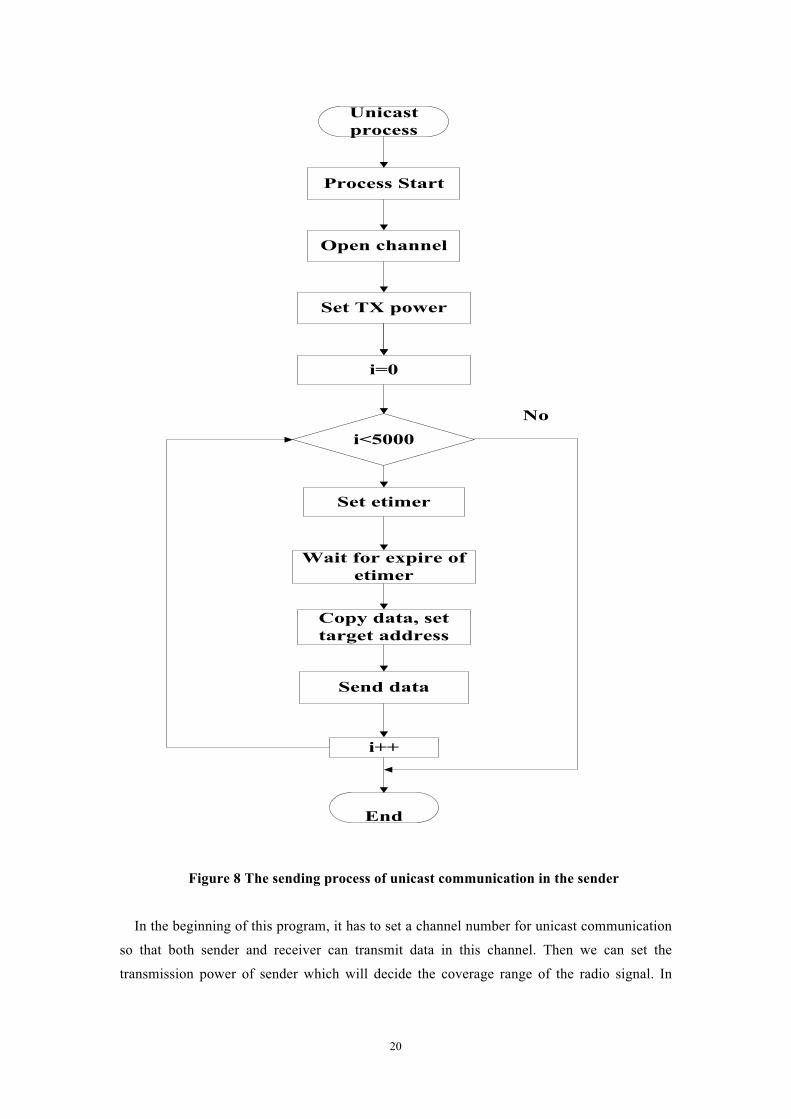
Figure 9 The callbacks function of receiver

Whenever the receiver node gets the data from the sender, it will invoke the callbacks

function automatically. The first time receiver node has got the data, the current system clock

time will be assigned to a temp variable. When the receiver gets the data again next time, we

22

use the current time minus the value of temp variable. So the exact transmission period time

between two data packets can be calculated. With the coffee file system of Contiki, it is easily

to store the period time into the text file. That is a convenient way for processing large

amount of data.

�

������������ ��������������������� ����� ���

�

We have accomplished many simulations with different system conditions and variant

program parameters. For the sake of better analysis of the effect of different conditions, they

are divided into several simulation groups.

�

� Simulation 1 Test of the effect of transmission power �

In order to figure out the effect of transmission power to the transmission period and

throughput in wireless sensor network, we have conducted six times simulations with

different transmission power (Tx power) from 2, 4, 8, 16, 24 and 31. There is a function for

setting the Tx power in COOJA. The value of Tx power can be changed from minimum value

1 to maximum value 31.

In the simulation, other parameters are kept be constant so they will not affect the

transmission period and throughput. The channel check rate is set to 32Hz/s. The length of

data packet is 60 bytes which includes the head part and data part. Meanwhile, the low power

X-MAC was used as the MAC protocol. Another parameter that may affect the transmission

period is packet generation rate. The frequency of data packet generation rate is set to very

high which means sender will transmit the data immediately when the receiver node is ready

to receive. So in this simulation, we can ignore its effect and only consider about the effect of

transmission power.

To avoid of the random interference or error inside the system, iteration method was used

to overcome this problem. The transmission process is repeated 1000 times to get more ac we

decide to use curate transmission period time. After the simulation, the receivers totally

received 1000 data packets from sender. Then all the transmission period time is stored in the

coffee file system because it is easy to read and write the data in text file. After getting all the

data, it is easy to use the Matlab software to deal with the data and draw the picture. The

figure is shown below.

23

Figure 10 ����������������� �������������������� ����������������������

The figure 10 shows the different transmission period time in the five tests with different

transmission power. The Matlab software was used to draw the five diagrams into one figure.

Because every transmission period time was drawn in one figure, so the subplots were looked

not so clearly. But it is easy to find that the period time was concentrated between 30ms to

35ms. The standard variances of every subplot were also calculated. They are 2.4499, 2.4495,

2.4495, 2.6285 and 2.4495 corresponding to the power 2, 4, 8, 16 and 31.

24

�

�

�������������� ������������������� �������������������� �������������������������� �

In the figure 11, X axis stands for the variant transmission power, Y axis stands for the

transmission period time. The average value of 1000 transmission period time has been

calculated to get more accurate data.

From the above figure, we can find that when the transmission power is set to 2, the

average value of transmission period is 32.002 ms, when the transmission power is 4, 8, 16,

24and 31, the average value of transmission period is 32 ms, 32 ms, 32.029 ms, 32.029 ms, 32

ms. It can be deduced from this result that even changing the transmission power, if the

receiver node is still in the coverage of signal from sender, it will not affect the transmitting

period time and throughput of wireless sensor networks.

According to the packet length and transmission period time, the throughput of network

can be calculated under these conditions. The throughput is about 15kbit/s. �

� Simulation 2 Test of the effect of data packet length �

In this simulation series, we mainly want to analyze if the data packet length will effect the

transmission period time.

The transmission power is set to 31 to make sure that receiver can get the data correctly.

Channel check rate is 16 Hz/s. Length of the data packet is changing from 40 bytes, 60 bytes,

80 bytes, 100 bytes and 120 bytes. The head of the data packet is 32 bytes, which includes the

address of the target receiver and CRC check. So I started my simulation from the data packet

25

length of 40 bytes. X-MAC is the simulation MAC protocol. Packet generation rate is set to

very high so I can ignore its effect.

In order to eliminate the random interference or error in the system, reiteration method

was used to overcome this problem. The transmission process repeated 1000 times to get

more accurate transmission period time. After simulation, the receiver totally got 1000 data

packets. There is no data packet loss in this simulation.

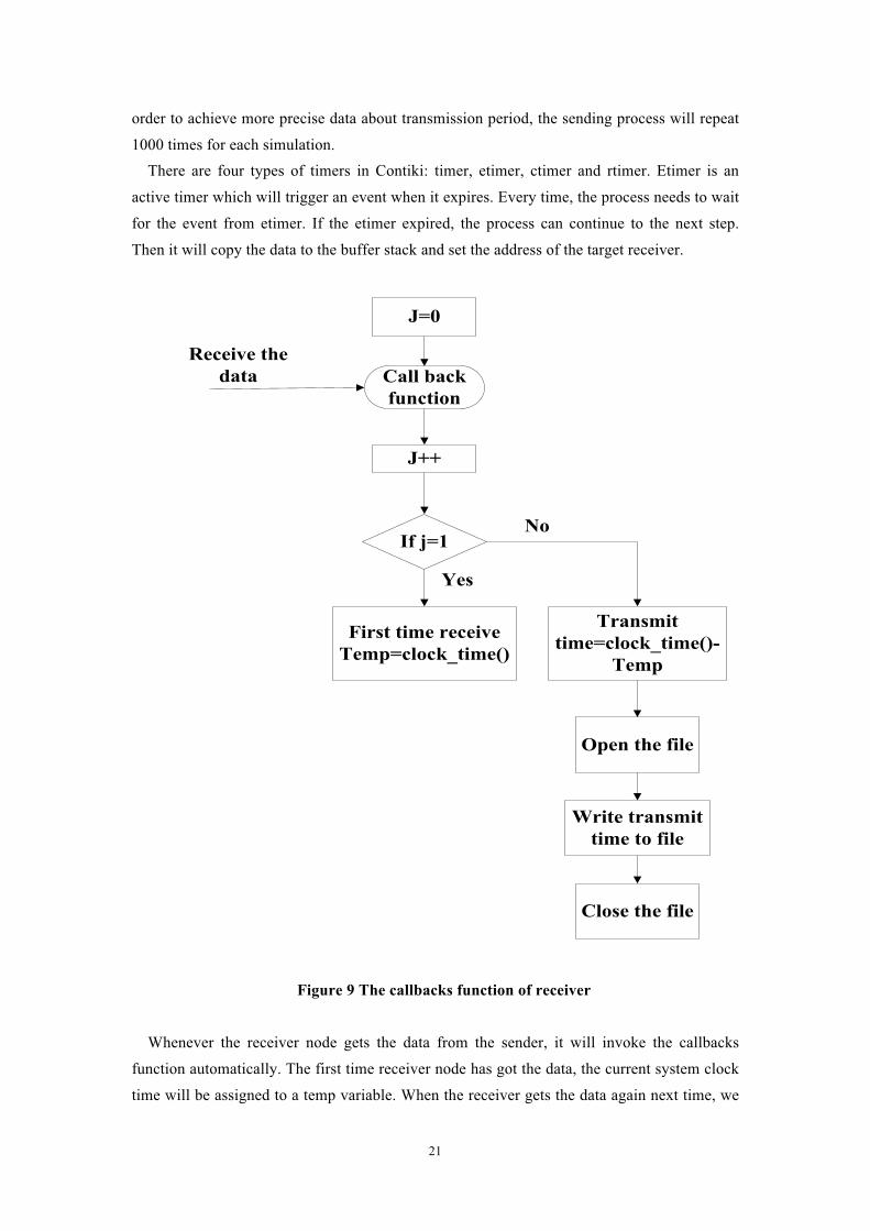
Figure 12 The transmit period time with variant data packet length

From the above figure, it is easy to be found that transmission period time concentrates

between 62ms and 66ms no matter the data packet length is 20 bytes or 120 bytes. The

standard variances of every subplot were also calculated. They are 2.5945, 2.5829, 2.5810,

12.5065 and 2.4701 corresponding to the data packet length 40 bytes, 60 bytes, 80 bytes, 100

bytes and 120 bytes.

In order to have clearer result, the average value of 1000 transmission period time is

calculated with the Matlab. In the later experiment, the figure only showing the average value

of transmission period time will be given.

26

��

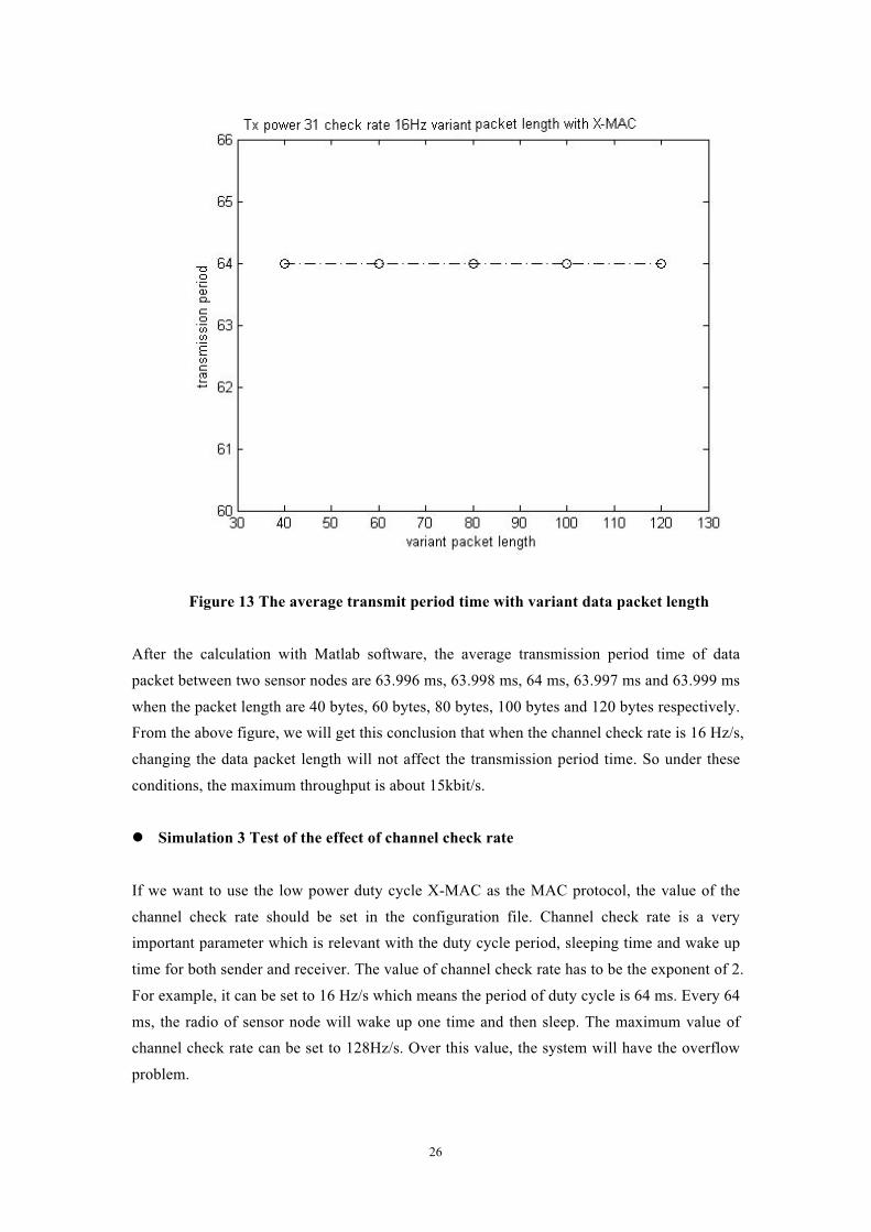
Figure 13 The average transmit period time with variant data packet length �

After the calculation with Matlab software, the average transmission period time of data

packet between two sensor nodes are 63.996 ms, 63.998 ms, 64 ms, 63.997 ms and 63.999 ms

when the packet length are 40 bytes, 60 bytes, 80 bytes, 100 bytes and 120 bytes respectively.

From the above figure, we will get this conclusion that when the channel check rate is 16 Hz/s,

changing the data packet length will not affect the transmission period time. So under these

conditions, the maximum throughput is about 15kbit/s.

�

� Simulation 3 Test of the effect of channel check rate �

If we want to use the low power duty cycle X-MAC as the MAC protocol, the value of the

channel check rate should be set in the configuration file. Channel check rate is a very

important parameter which is relevant with the duty cycle period, sleeping time and wake up

time for both sender and receiver. The value of channel check rate has to be the exponent of 2.

For example, it can be set to 16 Hz/s which means the period of duty cycle is 64 ms. Every 64

ms, the radio of sensor node will wake up one time and then sleep. The maximum value of

channel check rate can be set to 128Hz/s. Over this value, the system will have the overflow

problem.

27

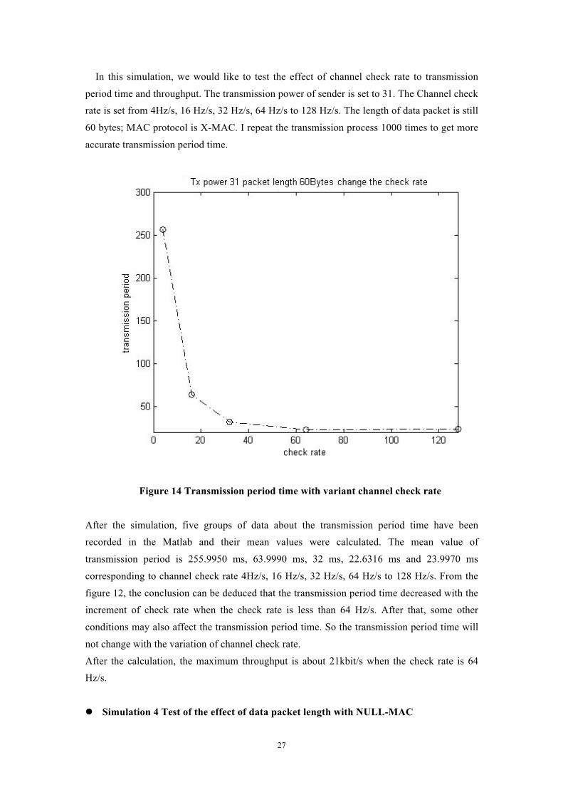
In this simulation, we would like to test the effect of channel check rate to transmission

period time and throughput. The transmission power of sender is set to 31. The Channel check

rate is set from 4Hz/s, 16 Hz/s, 32 Hz/s, 64 Hz/s to 128 Hz/s. The length of data packet is still

60 bytes; MAC protocol is X-MAC. I repeat the transmission process 1000 times to get more

accurate transmission period time.

��

Figure 14 Transmission period time with variant channel check rate

After the simulation, five groups of data about the transmission period time have been

recorded in the Matlab and their mean values were calculated. The mean value of

transmission period is 255.9950 ms, 63.9990 ms, 32 ms, 22.6316 ms and 23.9970 ms

corresponding to channel check rate 4Hz/s, 16 Hz/s, 32 Hz/s, 64 Hz/s to 128 Hz/s. From the

figure 12, the conclusion can be deduced that the transmission period time decreased with the

increment of check rate when the check rate is less than 64 Hz/s. After that, some other

conditions may also affect the transmission period time. So the transmission period time will

not change with the variation of channel check rate.

After the calculation, the maximum throughput is about 21kbit/s when the check rate is 64

Hz/s.

� Simulation 4 Test of the effect of data packet length with NULL-MAC

28

�

NULL-MAC is the other MAC protocol I used in the simulation. This is the simplest MAC

protocol which does not have the complicate mechanism like X-MAC to save the energy and

power consumption. So the radio of sender and receiver will keep open all the time. It can

transmit data much faster than X-MAC protocol. There is no channel check rate parameter in

NULL-MAC protocol.

What we are interested in the simulation of NULL-MAC protocol is the effect of data

packet length to transmission period time. In the previous simulation, the effect of packet

length with X-MAC protocol has already been simulated. We would also simulate the

application program with six variant data packet lengths from 20 bytes, 40 bytes, 60 bytes, 80

bytes, 100 bytes to 120 bytes.

The transmission power is set to 31. The transmission process repeated 1000 times in

sender to achieve more accurate delay time.

��

Figure 15 Transmission period time with variant data packet length under

NULL-MAC protocol �

After the simulation, six groups of data about the transmission period time have been

recorded in the Matlab and calculated their mean values. The mean values of transmission

period are 2.9980 ms, 3.9980 ms, 4.9880 ms, 5.8980 ms, 5.9980 ms and 6.9980 ms

29

corresponding to the data packet length from 20 bytes, 40 bytes, 60 bytes, 80 bytes, 100 bytes

to 120 bytes. The figure shows that with the increment of data packet length, the transmission

period time will increase as well. This is a difference between X-MAC and NULL-MAC

protocols. The maximum throughput under these conditions is about 137kbit/s. It can be

found that the transmission speed is much faster than the transmission with X-MAC protocol.

From the above figure, we also can find that when the data packet length changed from

80Bytes to 100Bytes, the transmission period time only changed a little. After analysis of the

figure and data, it can be deduced that because of the precision constraint, the minimum

transmission period time is 1 millisecond. So the system will calculate the round off for the

value. So no matter the value is 5.6ms or 6.3ms, it will round off to 6ms. That makes the little

change between 80bytes and 100bytes.

� Simulation 5 Test of the effect of data packet generation rate

In this group, the transmission period time and throughput in two hop (one sender, one relay, one receiver) wireless sensor network have been tested. In this simulation, there are three sensor nodes. The sender can only transmit the data to the relay node due to the distance and power constraint. This is the first hop. Then after receiving the data from sender, relay node transmits the data to the receiver node as soon as possible. That is the second hop. The transmission period in relay node and receive node will be calculated respectively.

The data packet length is 60 bytes. The transmission power is set to constant value 31 in

sender and relay node. Channel check rate of every node is 16Hz/s. The transmission period

time of both relay node and receive node will be record. The condition that is changing in this

simulation is data packet generation rate.

There is a parameter that we can set in the software, which can control the data packet

generation rate. This parameter is used in the etimer. If the program wants to run into the next

step, it needs to wait for an event. When the etimer count down from the value of parameter

to zero, it will trigger an event in the process. Then the program in sender can continue, and it

will store the data packet into the buffer and get ready to transmit data.

In this simulation group, the data packet generation rate of sender is set to five different

values: 1 data packet in 1 second, 10 data packets in 1 second, 50 data packets in 1second,

100 data packets in 1second and 1000 data packets in 1 second. The sender will repeat

transmission process 1000 times.

The transmission period time of relay node and receive node were drawn in two pictures.

For the convenience of display the transmission period, we took the logarithm of data

generation rate and use it as the X axis value.

30

��

Figure 16 Transmission period of relay node with variant packet generation rate �

The mean value of transmission period time with different generation rate has been calculated

respectively. The mean value of transmission period time of relay node is 1088 ms, 128.0661

ms, 64.001 ms, 63.9929 ms and 64.0042 ms corresponding to the packet generation rate 1

Hz/s, 10 Hz/s, 50 Hz/s, 100 Hz/s and 1000 Hz/s.

From the figure 16, we can find that the transmission period time will decrease with the

increment of packet generation rate at first. But after one value of generation rate, the

transmission period time will keep stable and not be affected. Since the value of transmission

period time is about 64 ms and channel check rate is 16 Hz/s, it can be deduced that it may be

affected by the channel check rate at that time.

The figure about the transmission period time in receiver node is showed below. After

comparing these two figures, maybe we can find the effect of the different packet generation

rate.

�

�

31

��

Figure 17 Transmission period of receiver node with variant packet generation rate �

The mean value of transmission period of receiver is 1088 ms, 127.7994 ms, 63.9990 ms,

64.001 ms and 64.0011 ms corresponding to the packet generation rate 1 Hz/s, 10 Hz/s, 50

Hz/s, 100 Hz/s and 1000 Hz/s. From the figure 17, we can find that this figure is the same as

the figure 16. So it is easy to get the some conclusion as before.

After calculation, the throughput of this network is about 7.5kbit/s when the channel check

rate is 16 Hz/s and packet generation rate is1000 Hz/s.

�

� Simulation 6 Test of the effect of data generation rate based on Poisson distribution�

In this simulation group, the effect of random discrete data packet generation rate based on Poisson distribution will be tested. Poisson distribution is a discrete probability distribution, which is used to express the probability of the number of events occurring in a fixed time. The equation below is the Poisson distribution function.

f(k; )=!

kek

λλλ−

(5)

λ is the expected number of occurrence during the interval time k is the number of occurrence of an event

32

In the Matlab, there is an internal Poisson distribution function

R = POISSRND (LAMBDA, M, N...) (6)

This function can be used to generate an array of random Poisson distribution data. This random data can be applied as the packet generation rate in the sender.

R=poissrnd (16, 1000, 1) (7)

The expected value λ is set to 16, here “1000, 1” means it will generate 1 column 1000 data.

The other conditions are set to be the same as before. The data packet length is 60 bytes. The transmission power is set to constant value 31 in sender and receiver. Channel check rate of every node is 16Hz/s. The condition that is changing in this simulation is data packet generation rate which is based on Poisson distribution. The figure about the transmission period time in receiver is shown below.

�

�

Figure 18 The transmission period time with packet generation rate based on Poisson

distribution

After calculation, the mean value of transmission period time is 119.5982 ms. From the figure

18, it can be found that due to the random of the packet generation rate, the transmission

period time will also change. �

�

� Simulation 7 Test of the transmission period time in multi-hop network

33

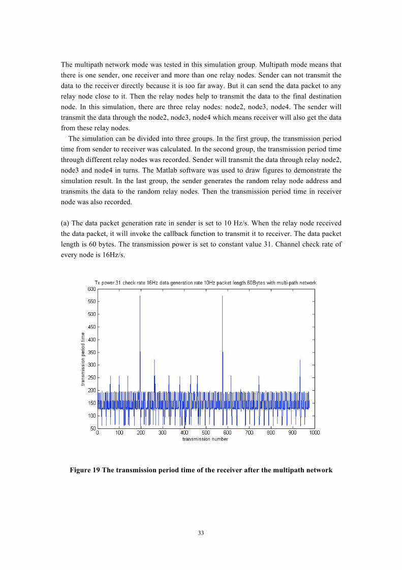
The multipath network mode was tested in this simulation group. Multipath mode means that there is one sender, one receiver and more than one relay nodes. Sender can not transmit the data to the receiver directly because it is too far away. But it can send the data packet to any relay node close to it. Then the relay nodes help to transmit the data to the final destination node. In this simulation, there are three relay nodes: node2, node3, node4. The sender will transmit the data through the node2, node3, node4 which means receiver will also get the data from these relay nodes.

The simulation can be divided into three groups. In the first group, the transmission period time from sender to receiver was calculated. In the second group, the transmission period time through different relay nodes was recorded. Sender will transmit the data through relay node2, node3 and node4 in turns. The Matlab software was used to draw figures to demonstrate the simulation result. In the last group, the sender generates the random relay node address and transmits the data to the random relay nodes. Then the transmission period time in receiver node was also recorded. (a) The data packet generation rate in sender is set to 10 Hz/s. When the relay node received the data packet, it will invoke the callback function to transmit it to receiver. The data packet length is 60 bytes. The transmission power is set to constant value 31. Channel check rate of every node is 16Hz/s.

Figure 19 The transmission period time of the receiver after the multipath network

34

After the calculation, the mean value of transmission period time is 144.0851 ms. From the

figure 19, it can be found that the transmission period time of the receiver is not so stable. The

receiver node may sometimes be affected by the interference of other nodes.

(b) In this group, sender transmitted the data packet through the relay node2, node3 and node4

in turns and the transmission period time in receiver was recorded. The other conditions are

set to be the same as before. The differences are that channel check rate of every node is

32Hz/s and the data packet generation rate is 20Hz/s. We have tested three groups and

calculate the transmission period time through different relay nodes.

Figure 20 The transmission period time through different relay node in the multipath

network

35

Figure 21 Transmission period time through different relay node in multipath network

Figure 22 Transmission period time through different relay node in multipath network

36

These three simulations were tested separately so the start sequence of sender, relay node and

receiver is different. From the above three figures, we can find that the transmission period

time from sender to receiver will differ through different relay node. But there is not one

certain path on which data is transmitted fast than other paths. The transmission period time is

only related with the start sequence of sensor nodes and this is randomly decided in the

simulation.

(c) The conditions are set to be the same as before. The differences are data packet generation

rate is 10Hz/s. Because the sender will generate the destination address randomly, so the three

relay nodes will have random amount of data packets. Two groups have been simulated. In

the first group, three relay nodes almost have the same amount data packets. In the second

group, there are more data packet transmitted through node2 than node3 and node4. The

figures are shown as follows.

Figure 23 The transmission period time randomly through different relay node in the

multipath network

37

Figure 24 The transmission period time randomly through different relay node in the multipath network

From these above two figures, we can get the same conclusion as before that the transmission

period time is not stable through different relay node. And there is no path on which data can

be transmitted faster than other path. The factor that will affect the transmission period time is

the start sequence of every node which is randomly decided by the COOJA simulator.

3.3 Field Test Field test of wireless sensor network is different from simulation in COOJA simulator. We have implemented the simulations with different system conditions and parameters in COOJA for both single hop and two hop networks. But all of these are accomplished in ideal environment. There is no hardware support, environment constraint and other interference. So it is estimated that there may be some difference in the result of field test compared with simulation test.

Since the COOJA simulator can emulate the Tmote Sky nodes very well, so the application programs used in the field test are exactly the same as the programs in the simulation. It can be transplanted to the real sensor node without any modification. Like the simulation test, the field test will also be divided into several groups to help analyze the test result.

38

Figure 25 The field test experiment platform In the above figure, it shows the real field test platform with five wireless sensor nodes of the multipath network. The receiver node is connected with the computer, so the test result can be print on the console. The three nodes in the middle are relay nodes. The sender can transmit the data through any relay node to the receiver. All the data packets are transmitted through the radio signal. � Field test group 1 Test of the effect of variant transmission power In the first field test group, the effect of transmission power to the transmission period and throughput was tested in the real sensor networks. The variable of transmission power was set to five different values: 4, 8, 16, 24 and 31.

As what we have done in the COOJA simulator, the other parameters were set to constant

values to avoid them changing the transmission period and throughput. The channel check

rate is set to 32Hz/s. The length of data packet is 60 bytes which includes the head part and

data part. Meanwhile, the low power X-MAC is used as the MAC protocol. The distance of

the sender and receiver is set to 1 meter. I repeated the transmission process 1000 times in

sender to achieve more accurate transmission period time.

From the experiment, we find that the transmission distance is greatly affected by the

transmission power of radio. When the transmission power is set to 2, receiver can not get the

data packet correctly from the sender which is located 1 meter away. That is why the first

39

value of transmission power is set to be 4 in the field test.�After the field test, I got five groups

data of transmission period time.

Figure 26 The transmission period time with variant transmission power

The above figure shows the result of the transmission period time with variant transmission power. Every subplot includes the value of 1000 transmission processes. From the figure, we can see that transmission period time mainly concentrate between 29ms to 36ms. The standard variances of every subplot were calculated with Matlab. They are 3.0755, 2.8142, 3.0457, 2.8968 and 2.8427 corresponding to the power 4, 8, 16, 24 and 31.

40

Figure 27 The average transmission period time with variant transmission power In the figure 27, Matlab was used to calculate the mean value of period time. The mean values of each group are 32.03 ms, 31.998 ms, 31.999 ms, 31.995 ms and 32.001 ms. If the mean values of transmission period time were drawn in one figure, it will like the above one. X axis is the variant transmission power of sender. Y axis is the transmission period. From the figure 27, it can be found that transmission period time is very stable even with different transmission power. � Field test group 2 Test of variant packet length with X-MAC protocol In this field test group, the transmission power is set to 31 to make sure that receiver can get

the data correctly. The channel check rate is 16 Hz/s. The length of data packet is changing

from 40 bytes, 60 bytes, 80 bytes, 100 bytes to 120 bytes. The head of the data packet is 32

bytes which includes the address of the target receiver and CRC check. So the simulations are

started from the data packet length of 40 bytes. X-MAC is the MAC protocol of wireless

sensor network. The data packet generation rate is set to be very high so its effect can be

ignored.

41

Figure 28 The transmission period time with variant packet length The above figure shows the result of 1000 transmission period time with different data packet length. From the figure, it can be found the value of transmission period time mainly concentrate between 62ms and 67ms. There are five subplots in the figure. The standard variances of every subplot were also calculated. They are 2.6503, 3.0256, 2.6728, 2.6798 and 2.6327 corresponding to the data packet length 40 bytes, 60 bytes, 80 bytes, 100 bytes and 120 bytes. In order to compare the result with different data packet length, Matlab is used to calculate the mean value of the 1000 transmission period time. The result is drawn in the next figure.

42

Figure 29 The average transmission period time with variant packet length From the above figure, we can see that the transmission period time is almost the same about 64 millisecond. The mean values of different data packet length are 63.997 ms, 63.997 ms, 63.991 ms, 63.996 ms and 64 ms. � Field test group 3 Test of the variant check rate with X-MAC protocol Channel check rate is a characteristic of X-MAC which decides the period of sleep and wake

up time for both sender and receiver.

In this experiment, the effect of channel check rate in transmission period time and

throughput was tested in real sensor network. The transmission power of sender is set to 31.

The parameter of channel check rate is set from 4 Hz/s, 8 Hz/s, 16 Hz/s, 32 Hz/s, 64 Hz/s to

128 Hz/s. The length of data packet is still 60 bytes. MAC protocol is X-MAC. The distance

is set to 1 meter. The transmission process repeated 1000 times to get more accurate

transmission period time.

43

Figure 30 The transmission period with variant channel check rate The mean values of transmission period are 256.001ms, 127.994ms, 63.996ms, 32.001ms, 22.307ms and 23.049ms corresponding to channel check rate 4Hz/s, 8Hz/s, 16 Hz/s, 32 Hz/s, 64 Hz/s to 128 Hz/s. So the throughput is about 21.5kbit/s when the check rate is 64 Hz/s. From the above figure, it can be found that the transmission period time will decrease with the increment of channel check rate in proportion before 64 Hz/s. Then the transmission period time do not decrease with the increase of channel check rate. We think that this is the effect of some other constraint factors. � Field test group 4 the effect of variant data packet length NULL-MAC protocol is totally different with X-MAC protocol we have used in the test

before. This is the simplest MAC protocol which does not have the complicate mechanism,

like X-MAC, to save the energy and power consumption. So the radio of sender and receiver

will keep turn on all the time. It can transmit data much faster than X-MAC. There is no

channel check rate parameter in NULL-MAC.

We would like to test the effect of data packet length to transmission period with

NULL-MAC protocol. In the previous test, the similar experiments with X-MAC protocol

have been accomplished. The application program was tested with six variant data packet

lengths in real sensor nodes from 20 bytes, 40 bytes, 60 bytes, 80 bytes, 100 bytes to 120

bytes.

44

The transmission power is set to 31. The distance is still set to 1 meter. The transmission

process repeated in sender 1000 times to achieve more accurate transmission period time.

Figure 31 The transmission period time with variant data packet length with NULL-MAC protocol After the calculation, the mean values of transmission period time with different data packet length are 3.0 ms, 4.0 ms, 5.004 ms, 5.9 ms, 6.0 ms and 7.0 ms. The maximum throughput under this condition is about 137kbit/s when the length is 120 byte. From the figure 31, we can find that the transmission period time increase with the increment of the data packet length under NULL-MAC protocol. From the packet length 80bytes to 100bytes, the transmission period time just change a little. It also has the round off problem here. � Field test group 5 Test of different distance between sender and receiver

In this test, the transmission power is set to 31 to make sure that receiver can get the data even

in far distance. Data packet length is set to 60 bytes. MAC protocol is NULL-MAC. The

distance between sender and receiver is set to 1 meter, 2 meters, 4 meters and 8 meters.

45

Figure 32 The effect of variant test distance to transmission period

The mean value of every group of transmission period time is 7.0 ms, 7.0 ms, 7.0 ms and 7.0 ms. From the above figure, we can see that the transmission period time is not relevant to the transmission distance if the receiver still can get the data packet from sender correctly. It is easy to understand. According to the knowledge we have, we know that the transmission speed of the electromagnetic wave in air is very fast, about 30 km/s. So even we moved the sender and receiver very far away, it will not have very apparent effect to the transmission period time. � Field test group 6 Test of environment interference One of the significant differences between wireless sensor network simulation and Field test

is the interference from other radio source in the environment. The interference comes from

two parts, the electromagnetic interference and barrier block. The effect of electromagnetic

interference to transmission period time will be firstly tested.

There are various radio sources in the room that can interfere the transmission of data in

wireless sensor network. The wireless sensor network is working on the unlicensed 2.4GHz

RF worldwide frequency band which is also the frequency bond for Wireless Local Area

Network (WLAN). The wireless router and computer or cell phone with Wi-Fi are the main

interference source. In this field test, the tests are separated into two groups. In the first group,

there are several cell phones and computers connecting to the internet with Wi-Fi around the

46

sensor nodes. In the other group, there is no digital equipment and signal around the sensor

nodes.

The other test conditions are the same as before. The transmission power is set to 31 to

make sure that receiver can get the data correctly. Channel check rate is 16 Hz/s. The length

of data packet is 60 bytes. X-MAC is the MAC protocol of wireless sensor network. The data

packet generation rate is set to very fast so we can ignore its effect.

We tested the data transmission five times for each group. Each time, the sender

transmitted 1000 data packets to receiver in order to achieve accurate value of transmission

period time. Then I use the Matlab to calculate the mean value of each time.

Figure 33 The effect of interference with X-MAC After the calculation, the normal transmission period without interference is 64 ms. The mean transmission period time with interference are: 64.1324 ms, 63.999 ms, 64.3842 ms, 64.703 ms and 64.248 ms. Without the interference, the throughput of the system is about 7.5kbit/s. With the interference, the throughput decrease to 7.46kbit/s. From the above figure, we also can find that transmission period time with interference is longer. After this test, the conclusion can be deduced that interference from other radio sources will affect the transmission period time of wireless sensor network. � Field test group 7 Test of the effect of the wall block

47

Another interference of the radio signal is the barrier block. Since the wireless sensor network work on the 2.4 GHz frequency bond, the radio signal is microwave. Microwave is not good at diffracting when something blocks the transmission route. If we conducted field tests in the house, the wall is the main barrier that will block the microwave signal.

In this test, NULL-MAC is the MAC protocol. The distance is set to four meters. The Data

packet length is 120 bytes. The transmission power is set to 31 to enable receiver to get the

data. The field tests are divided into two groups and four test times for each group. One is

tested with wall, the other one without wall. In every test, the sender will transmit 1000 data

packets to achieve more accurate delay time.

Figure 34 The effect of wall block to the transmission period We have tested four times for each group and calculated the average value. The transmission period time are 7.1833 ms, 7.3932 ms, 7.6579 ms and 7.4909 ms, if there is a wall between sender and receiver. The throughput is about 129.2kbit/s. But if there is no wall, the transmission period time are 7.0221 ms, 7.001 ms, 7.007 ms and 7.007 ms. The throughput is about 137kbit/s. So the throughput is higher than one in the test with the wall block. From this result, it can be deduced that the wall will block the transmission of radio signal, so it will affect the transmission period time and throughput. � Field test group 8 Test of variant packet generation

48

In this test group, the data packet length is 60 bytes. The transmission power is set to constant

value 31 in sender, relay node and receiver. Channel check rate of every node is 16Hz/s. The

transmission period time of both relay node and receive node is recorded. The condition that

is changing in this simulation is data packet generation rate. The sender generation rate was

set to four different values: 1data packet in 1 second, 10 data packets in 1 second, 100 data

packets in 1second and 1000 data packets in 1 second. The sender will repeat transmission

process 1000 times.

Figure 35 The effect of data packet generation rate on transmission period time The mean values of transmission period of node2 (relay node) are 1088.3ms, 128.7ms, 64.245ms and 63.997ms corresponding to data packet generation 1Hz/s, 10Hz/s, 100Hz/s and 1000Hz/s. The mean values of transmission period of node3 (receiver node) are 1090.4ms, 128.67ms, 64.191ms and 63.998ms.

From the above figure, we can know that the transmission period of relay node and receiver node are very similar. Data packet generation rate will affect the transmission period time. But after one value, the transmission period time will not decrease with the increment of data packet generation rate due to some other effective factors. � Field test group 9 Test of data packet generation rate based on Poisson distribution

49

In this field test group, we studied the effect of random discrete data packet generation rate based on Poisson distribution. This field test group is corresponding with the simulation group6. All the test internal conditions are set to be the same as simulation group6. The expected

value λ is set to 16. The data packet length is 60 bytes. The transmission power is set to

constant value 31 in sender and receiver. Channel check rate is 16Hz/s. The distance between

sender and receiver is 1 meter.

The condition that is changing in this test is data packet generation rate in sender which is

based on Poisson distribution. The figure about the transmission period time in receiver is

listed below.

��

Figure 36 The transmission period time with packet generation rate based on Poisson

distribution

After calculation, the mean value of transmission period time is 118.9539 ms. From figure 31,

we can find that due to the random packet generation rate, the transmission period time will

also change with the different packet generation rate. The average throughput under this

condition is about 4kbit/s.

� Field test group 10 Test of the transmission period time in multi-path network

50

This real field test group is corresponding to the multipath simulation group. There are one sender, one receiver and more than one relay nodes. Sender can not transmit the data to the receiver directly because it is too far away. But it can send the data packet to any relay node close to it. In this field test, there are also three relay nodes: node2, node3 and node4. Then the relay nodes help to transmit the data to the final destination node.

The field test was divided into two groups. In the first group, the sender will transmit the data to node2, node3 and node4 in turns which means receiver will also get the data from relay nodes in turns. In the second group, the sender generates the random destination address and transmits the data to the random relay node firstly. The transmission period time through different relay nodes was recorded and Matlab is used to draw figures to demonstrate the field test result.

Figure 37 The transmission period time through different relay node in the multipath

network

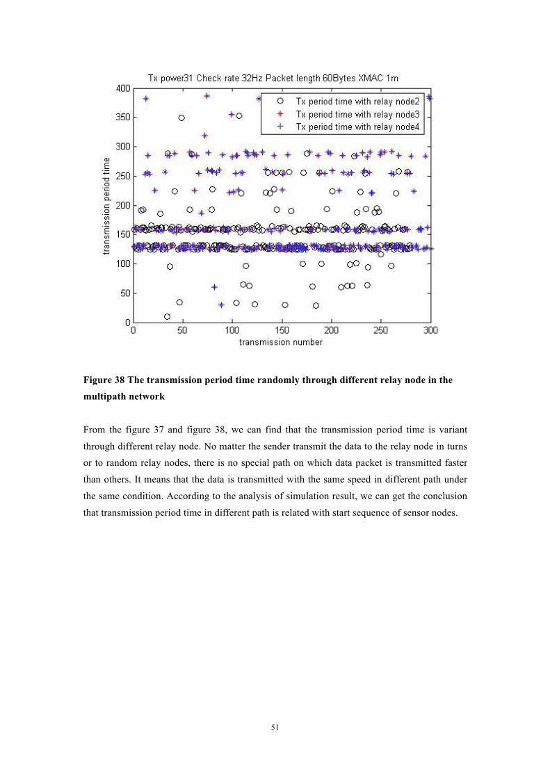
51

Figure 38 The transmission period time randomly through different relay node in the multipath network

From the figure 37 and figure 38, we can find that the transmission period time is variant

through different relay node. No matter the sender transmit the data to the relay node in turns

or to random relay nodes, there is no special path on which data packet is transmitted faster

than others. It means that the data is transmitted with the same speed in different path under

the same condition. According to the analysis of simulation result, we can get the conclusion

that transmission period time in different path is related with start sequence of sensor nodes.

�

�

52

Chapter 4

Comparison and Conclusion of test

In Chapter 3, we have implemented several different simulation groups of networks and

tested the transmission period time of single hop, two hop and multipath networks. After the

simulations, a large amount of data about transmission period time has been obtained. The

throughput of the network under some specific conditions has also been calculated. In order to

compare with the result of simulation, we have also executed ten groups of field test and

drawn all the figures with Matlab software.

In this chapter, we will compare the experiment data from simulation and field test. Then

the result of the transmission period time from the simulations and field tests will be analyzed.

After that, some conclusions about the whole simulation and field tests are summed up.

4.1 Comparison of experiment data The simulation test can be divided into 6 groups. They are classified according to the different

simulation conditions, for example different transmission power, different channel check rate

of X-MAC, different data packet length, different packet generation rate and different MAC

protocols. After analyzing the transmission period time under different conditions, It will be

easy for us to know which condition can affect the data packet transmission period and

throughput in WSNs.

The same as the simulation tests, the field tests also can be divided into several groups. Some

field tests are corresponding with the simulation tests. �

�The first group

53

Figure 39 Comparison of the simulation test and field test with variant Tx power

In the first group, it is a single hop wireless network. We changed the transmission power of

the sender and set the other conditions to be constant value. From the figure 39, it can be

found that the transmission period time is very stable about 32 ms no matter how strong or

weak the transmission power is. But the precondition is that receiver can receive the data

correctly and successfully.

In the field test result, we also can find that the transmission period is about 32 ms from the

figure 39. After analysis of the result, it can be summarized that the transmission power will

not affect the transmission period time. Real sensor node test has the same result as

simulation tests.

��The second group

54

Figure 40 Comparison of the simulation test and field test with variant packet length

This group is also implemented in the single hop network and with X-MAC protocol. We

changed the data packet length to several different values and set the other condition to be

constant value. From the simulation and field test result, we can know that transmission

period time is about 64 ms when the channel check rate is 16 Hz/s. The transmission period

time will not change with the different data packet length. So we can get this conclusion that

data packet length will not affect the transmission period time if it is tested in X-MAC and

with low channel check rate.

�The third group

In this group, the channel check rate is changed in X-MAC protocol and other conditions are

set to be stable. The mean values of transmission period are 256.001ms, 127.994ms,

63.996ms, 32.001ms, 22.307ms and 23.049ms corresponding to channel check rate 4Hz/s,

8Hz/s, 16 Hz/s, 32 Hz/s, 64 Hz/s to 128 Hz/s.

55

From the simulation and field test results, I can find that when check rate is less than 64 Hz/s,

the transmission period decreased with the increment of channel check rate and in inverse

proportion. So we can get the conclusion that the channel check rate will affect the

transmission of data.

When the channel check rate is set to 64 Hz/s and 128 Hz/s, although the transmission period

time is less than it in 32 Hz/s, the period time didn’t change in the same ratio as the change of

channel check rate. After analyzing this situation, we think the reason is that the channel

check rate is too high for the sender and receiver. Sender can not finish the whole

transmission mechanism of X-MAC protocol in very short time with receiver. So when the

channel check rate increases, it will not shorten the transmission period time in the same ratio.

Some other factors constraint the transmission period time and throughput of the network.

�The fourth group

In this group, all the simulation tests and field tests are implemented with NULL-MAC

protocol. We changed the data packet length again in this group and set the other condition

static. From the figure 15 and figure 31, we can find that the transmission period time will

increase with the increment of the data packet length in both simulation and field test. From

this phenomenon, the conclusion can be deduced that increasing the length of the data packet

will also increase the time of receiving the data packet. So it will affect the transmission

period time with NULL-MAC protocol. Because it is one simple MAC protocol without any

complicated mechanism.

�The fifth group

In this group, the transmission process with different data packet generation rate is tested. It is

tested in the two-hop network with X-MAC protocol. The channel check rate is set to 16 Hz/s

and other conditions are constant values. In the sender, the packet generation rate is set to 1

Hz/s, 10 Hz/s, 20 Hz/s, 100 Hz/s, 1000Hz/s and transmission period time is 1088ms,

128.0661ms, 64.001ms, 63.9929ms and 64.0042ms.

From the data, we can find that when the packet generation rate is 1 Hz/s and 10 Hz/s, the

transmission period will decrease with the increment of packet generation rate. From this

phenomenon, we can deduce the conclusion that the packet generation rate will affect the

transmission period time. But it is very stable when the generation rate is 20 Hz/s, 100Hz/s

and 1000Hz/s. It is estimated that when the packet generation rate is too fast, the transmission

period time will be constrained by the channel check rate. Because the channel check rate is

16Hz/s, so the transmission period time is about 64 ms no matter the generation rate is 20

Hz/s, 100Hz/s or 1000Hz/s.

56

�The sixth group

In this group, the effect of variant distance between sender and receiver has been tested. This

group was tested in the real field with wireless sensor nodes and NULL-MAC protocol. With

the constraint of the space, the distance was only tested about 1 meter, 2 meters, 4 meters and

8 meters.

From the figure 32, we can see that the transmission period time is about 7 ms and very stable.

So we conclude that the distance is not the condition that will affect the transmission period

time if the receiver can get the data under this condition. This result is coincident with the

theory. Because the transmission speed of radio signal is very fast, so even you change the

distance between sender and receiver, it is still impossible to detect the tiny difference.

�The seventh group

This field test group is implemented in indoor environment. With this test, we would like to

know that if the wall or door will block the radio signal and affect the transmission period

time of data. All the system internal conditions are set to be constant value and the concrete

wall separated the sender and receiver. Then we compared this test with the one without wall

block.

From the figure 34, we will find that compared with no block situation, the transmission

period time between sender and receiver is longer when the signal from sender is blocked.

After analysis of the data packet that receiver got, we found that receiver will also lose some

of the data packets in the transmission process. These two reasons make the throughput of the

network is lower than the test without wall block.

�The eighth group

This group is used to test the effect of the interference from the other wireless signals in the

environment. All the system internal conditions are set to be stable and the data transmission

period time is tested with the distance 1meter. From the figure 33, we can know that when we

put the cell phone and Wi-Fi spot around the sensor nodes, the transmission period time is

longer than the test without the interference.

Then conclusion can be deduced that the electromagnetism interference will affect the

transmission period time and increase the packet loss rate. Thus it will decrease the

throughput of the system.

� The ninth group

In this test group, a five nodes multipath wireless network in the same environment was

simulated and implemented. With these tests, we want to know about the transmission period

time in receiver through different relay nodes. Another research point is that if the data is

57

successfully relayed by the relay node. The simulation result is showed in the figure 19, 20,

21, 22, 23, 24 and the field test result is showed in the figure 37 and 38.

From the simulation figures, we can find that the transmission period time is different with

different relay nodes and it is not stable. But we can not find one path on which data is

transmitted faster than other path. The transmission period time is randomly decided by the

start sequence of every node. Because the simulation repeated three times and every time

COOJA would generate a random start sequence for every node.

From the field test figures, we also can get the same conclusion that in the same environment,

the transmission period time of data packet through different relay node depends on the start

sequence of nodes.

4.2 Conclusions of the test

From the above analysis and comparison, we can sum up these conclusions as follows.

First, the transmission power of the sender node will not affect the transmission period time

of data packet if the receiver will not lose the data packet.

Second, the data packet length will not affect the transmission period time if the channel

check rate is very low. But it will be affected if the sensor nodes work on the NULL-MAC

protocol or when the channel check rate is high in X-MAC protocol.

Third, the channel check rate in X-MAC protocol will affect the transmission period time. If

we increase the check rate, the transmission period time will also decrease the same

proportion. After a threshold value of the channel check rate, the transmission period tune

will not decrease any more because of the X-MAC mechanism.

Fourth, the data packet generation rate will affect the transmission period time when the

packet generation rate is slower than the channel check rate. But when the packet generation

rate is faster than the channel check rate, the transmission period time will be constrained by

channel check rate and will not decrease with the increment of packet generation rate any

more.

Fifth, the distance between sender and receiver will not affect the transmission period of data

packet. But the precondition is that receiver can get the data from the sender successfully

Otherwise, it will cause the packet loss and change the transmission period.

58

Sixth, if there are wall or doors blocking the transmission of the signal, it will make the data

packet lost and affect the transmission period time and throughput.

Seventh, some radio signal from electromagnetism source will interfere the transmission of

data between sender and receiver. So it will cause data packet loss and affect the transmission

period and throughput.

Eighth, compared with the X-MAC protocol, the system using NULL-MAC protocol can

transmit the data faster.

Ninth, in a multipath network, if every path is settled in the same environment, the

transmission period time of data packet through different relay nodes is randomly decided by

the system and depends on the start sequence of nodes.

59

Chapter 5

Result and future work

5.1 Result The wireless sensor networks experiment platform which includes the simulation test and field test has been designed to test the data transmission period and throughput in WSN. The reason that we would like to test the throughput of the network is that throughput will decide the application area of the wireless sensor network. After a large number of experiments, a lot of transmission period time data with different test conditions was obtained.

After the analysis of transmission period time, some conclusions about the effect of different conditions were summed up. These conditions include system internal conditions and environment conditions which will affect the transmission period time and throughput of the wireless sensor networks. After the comparison of simulation transmission period time with real field test, we found that the COOJA simulator performs very well and the code can be transplanted to the sensor node without any modification. The result of the simulation is the same as the field test.

5.2 Future Work In this thesis, one experimental platform testing the transmission period time and throughput of wireless sensor networks has been built up. But the test conditions and network topology modes are limited due to the time and sensor nodes. There are still some transmission modes that we haven’t tested, for example best effort multi-hop unicast, hop-by-hop reliable mesh routing. It is thought that these modes should be tested in the future work. That can help people to understand the mechanism in more complicated wireless sensor networks.

What’s more, another important point of the wireless sensor network is power consumption. Power consumption decides the duration time of the WSN system. In order to make it work long time, users have to research and develop some methods to save the power consumption. If we can test the power consumption value of every part of the WSN, then we can find the information about the power consumption of every component. So in the future work, we are going to study how to save the energy and try to find a method to save the energy.

60

Reference

[1]CC2420 data sheet. http://www.ti.com

[2]CM5000 mote datasheet. http://www.advanticsys.com/cm5000.html

[3]Contiki Operating System http://contiki-os.blogspot.com

[4]Zigbee alliance. http://zigbee.org

[5]I. Akyildiz, W. Su, Y. Sankarasubramaniam, and E. Cayirci. A survey on sensor networks, 2002. IEEE Communication. Magazine. 40.

[6]A. Dunkels. Rime – a lightweight layered communication stack for sensor networks. Jan. 2007.

[7] AdamDunkels, Bj¨orn Gr¨onvall, and Thiemo Voigt. Contiki - a lightweight and flexible operating system for tiny networked sensors. In Proceedings of the First IEEE Workshop on Embedded Networked Sensors (Emnets-I), Tampa, Florida, USA, November 2004.

[8] Adam Dunkels. Full TCP/IP for 8 Bit Architectures. In Proceedings of the First ACM International Conference on Mobile Systems, Applications and Services (MobiSys 2003), San Francisco, May 2003.

[9]Adam Dunkels, Fredrik ¨Osterlind, and Zhitao He. An adaptive communication architecture for wireless sensor networks. In Proceedings of the Fifth ACM Conference on Networked Embedded Sensor Systems (SenSys 2007), Sydney, Australia, November 2007.

[10] Neil Gershenfeld, Raffi Krikorian, Danny. The internet of things. Cohen Scientific American 291:44, 76-81, 10/2004.

[11] S. Bhatti, J. Carlson, H. Dai, J. Deng, J. Rose, A. Sheth, B. Shucker, C. Gruenwald, A. Torgerson, and R. Han. Mantis os: An embedded multithreaded operating system for wireless micro sensor platforms. ACM/Kluwer Mobile Networks & Applications (MONET), Special Issue on Wireless Sensor Networks, 10(4):563–579, August 2005.

[12] J. Polastre, J. Hill, and D. Culler. Versatile low power media access for wireless sensor networks. In The Second ACM Conference on Embedded Networked Sensor Systems (SenSys), pages 95�107, November 2004.

[13] Michael Buettner, Gary V. Yee, Eric Anderson, and Richard Han. X-mac: a short preamble mac protocol for duty-cycled wireless sensor networks. In SenSys ’06: Proceedings of the 4th international conference on Embedded networked sensor systems, pages 307–320, New York, NY, USA, 2006. ACM Press.

[14] P. Levis. TOSSIM: Accurate and Scalable Simulation of Entire TinyOS Applications. In Proceedings of the First ACM Conference on Embedded Networked Sensor Systems (SenSys 2003), 2003.

61

[15] IEEE P802.15.4 Working Group for WPAN, Cluster Tree Network, April 2001.

[16] W. Ye, J. Heidemann, and D. Estrin. An energy efficient mac protocol for wireless sensor networks. In 21st International Annual Joint Conference of the IEEE Computer and Communications Societies (INFOCOM�02), New York, NY, USA 2002.

[17] T. van Dam and K. Langendoen. An adaptive energy efficient mac protocol for wireless sensor networks. In 1st ACM Conference on Embedded Networked Sensor Systems (SenSys), pages 171�180, 2003.

62

Appendix A In this part, I explained step by step how to simulate the Coniki programs in the COOJA simulator. 1 Start COOJA Open a terminal window in the Linux Go to the COOJA directory, compile and start COOJA:

cd contiki-2.x cd tools/cooja ant run

2 Create a Simulation We can create a new simulation via the menu.

• Click menu item: File, New Simulation.

• Enter a Simulation title, and click Create.

We have now created a simulation in COOJA. However, the simulation does not contain any nodes yet. To add nodes we need to first create a node type, and then add nodes to the simulation. 3 Create a Node Type

• Click menu item: Mote Types, Create mote type, Sky Mote Type.

We need to select to emulate Tmote Sky nodes, and then select what Contiki program to simulate.

• Enter a Description

• Click Browse, and navigate to programs examples/rime/example-unicast.c

• Click Compile to start compiling the Contiki program

When the compilation finishes:

• Click Create.

We have now created a simulation with a single node type. Before finally starting to simulate, we need to add nodes belonging to this node type.

4 Add Simulated Nodes

63

• Menu item: Motes, Add motes of type,

Add 2 nodes:

• Enter 2, and press Create and Add.

Five nodes are added to the simulation, randomly located in the XY-plane.

5 Start Simulating A number of plugins are automatically started. These, and more plugins, can be accessed via the plugins menu:

• Menu items: Plugins, Log Listener and Plugins, Simulation visualizer.

Then In the Control Panel:

• Click Start to start the simulation.

Then the node serial data will appear in the Log Listener. 6 Save, Load and Reload COOJA allows for saving and loading simulation configurations. To save your current simulation:

• Click menu item: File, Save simulation.

Simulations are stored with the file extensions “.csc”. To later load a simulation:

• Click menu item: File, Open simulation, Browse.... Select a simulation configuration.

64

Appendix B In this part, I explained step by step how to run the programs in the real sensor nodes. 1 Open a Terminal Window After logging in the Linux, click on the terminal icon to start a terminal window. 2 Burning node IDs to EEPROM

To compile and run this program, go into your project directory and run

make burn-nodeid.u nodeid=X

Where X is the node ID that will be burned into EEPROM. The Node id will be the node address used in the program.

3 Connect the Tmote Sky Connect Tmote Sky node to the computer with a USB port. The Tmote Sky will appear in the top of the Instant Contiki (VMware Player) window with the name “Future Technologies Device”. Click on the name to connect the Tmote Sky to Instant Contiki.

4 Compile the program and upload In the terminal window, go to the program directory, Compile and upload the program on the Tmote Sky:

make example-unicast-test.upload TARGET=sky

Wait for the compilation and uploading procedure to finish. During the uploading the Tmote Sky should quickly flash the red LEDs next to the USB connector.

5 Run on the Tmote Sky View the program output in your laptop screen:

make login TARGET=sky

Press the reset button on the Tmote Sky and start the program

Then it will print The Contiki boot-up code the program result on the screen. Press Ctrl+C to quit.