Design and Analysis of a Compliant Shoulder Mechanism for Assistive Exoskeletons DMS4 Master Thesis Group 4 Aalborg University Design of Mechanical Systems

Welcome message from author
This document is posted to help you gain knowledge. Please leave a comment to let me know what you think about it! Share it to your friends and learn new things together.
Transcript

Design and Analysis of a CompliantShoulder Mechanism for Assistive
Exoskeletons
DMS4 Master Thesis
Group 4
Aalborg University
Design of Mechanical Systems

Copyright © Aalborg University 2021

Design of Mechanical SystemsAalborg Universityhttp://www.aau.dk
Title:Design and Analysis of a Compliant Shoul-
der Mechanism for Assistive Exoskeletons
Theme:DMS 4 Project
Project Period:Spring Semester 2021
Project Group:4
Participant(s):
Rohan Sameer Desai
Alexandros Marios Ekizoglou
Felix Balser
Supervisor(s):Shaoping Bai
Copies: 1
Page Numbers: 139
Date of Completion:3/6/2021
Abstract:
In this thesis the design and analysis of
a passive exoskeleton to assist the elderly
and workers for overhead tasks are pre-
sented. The scope of the exoskeleton is
to compensate for the gravitational forces.
The exoskeleton consists of a spherical
shoulder mechanism and a passive variable
stiffness mechanism. Both mechanisms
are described and further ideas are pre-
sented. Numerical, analytical and exper-
imental analyses of the variable stiffness
mechanism are carried out and compared.
Furthermore, topology optimisation is per-
formed to reduce weight. The exoskele-
ton focuses on assistance in the sagittal
plane, but due to the properties of the mod-
ules, also motion in different planes is sup-
ported. The final design compensates for
50% of the gravitational torque of the arm
with the elbow stretched.

The content of this report is freely available, but publication (with reference) may only be pursued due to agree-
ment with the author.
Preface
The report is written by DMS4 Group 4 from Aalborg University in the period February 1st,
2021 to June 3, 2021, with supervising by Shaoping Bai.
We would like to thank Shaoping Bai for knowledgeable supervising, for providing help and
information for the project. We also want to thank Zhongyi Li and the workshop in Fibiger-
stræde 14 for their help in manufacturing of the exoskeleton and providing equipement that
was used in the experiment.
Reading guide
This report uses the reference style APA. Source references will appear like the following:
[Author, Year]. The bibliography can be found at the end of the report followed by the ap-
pendices. If a larger section is based on a specific reference, this reference will be stated
explicitly at the beginning. The reference is displayed directly if specific statements, data or
figures are used for an external source. If no source is given, the material is generated by the
authors.
The numbering of figures, tables and equations is done by first stating the number of the
chapter they appear in, a full stop and the incremented number of elements of the same class.
For instance, the third element of a class in the fifth chapter is denoted as 5.3. Each table and
figure have a short description next to the numbering underneath the element. Equations are
numbered in the same scheme. The number is enclosed in brackets, that is (1.1) and is given
at the right next to or closely under the equation.
The appendices appear after the bibliography with a capital letter instead of a chapter
number. Sections and subsections are numbered with the capital letter of the appendix they
belong to and the number of the section or subsection. A.1.1, A.1.2 and A.2 are examples.
v
Contents
Preface v
1 Introduction 11.1 Range of Motion . . . . . . . . . . . . . . . . . . . . . . . . . . . . . . . 2
1.2 Passive Upper Limb Exoskeletons Applications . . . . . . . . . . . . . . . 3
1.3 Background of Existing Passive Upper Limb Exoskeletons . . . . . . . . . 3
1.3.1 Paexo . . . . . . . . . . . . . . . . . . . . . . . . . . . . . . . . . 4
1.3.2 EksoVest . . . . . . . . . . . . . . . . . . . . . . . . . . . . . . . 4
1.3.3 EVO . . . . . . . . . . . . . . . . . . . . . . . . . . . . . . . . . 5
1.3.4 MATE-XT . . . . . . . . . . . . . . . . . . . . . . . . . . . . . . 6
1.3.5 Hyundai Vest Exoskeleton . . . . . . . . . . . . . . . . . . . . . . 6
1.3.6 Comparison of Existing Upper Limb Exoskeletons . . . . . . . . . 7
1.4 Background of Existing Shoulder Joint Mechanisms . . . . . . . . . . . . . 8
1.4.1 Double Parallelogram Linkage . . . . . . . . . . . . . . . . . . . . 8
1.4.2 Compact 3-DOF Scissors Shoulder Mechanism . . . . . . . . . . . 9
1.4.3 Four-bar Based Poly-Centric Shoulder Linkage . . . . . . . . . . . 10
1.4.4 Other Existing Shoulder Joint Mechanisms . . . . . . . . . . . . . 10
1.5 Problem Formulation . . . . . . . . . . . . . . . . . . . . . . . . . . . . . 12
1.6 Problem Approach . . . . . . . . . . . . . . . . . . . . . . . . . . . . . . 13
2 Modeling of the Exoskeleton 152.1 VSM Modeling . . . . . . . . . . . . . . . . . . . . . . . . . . . . . . . . 15
2.2 AAU’s Scissors Shoulder Mechanism . . . . . . . . . . . . . . . . . . . . 18
2.2.1 Kinematics of the SSM . . . . . . . . . . . . . . . . . . . . . . . . 19
2.2.2 Design Limitations . . . . . . . . . . . . . . . . . . . . . . . . . . 22
2.2.3 SSM provided by AAU . . . . . . . . . . . . . . . . . . . . . . . . 25
vi
Contents Aalborg University
3 Assistance in the Sagittal Plane 273.1 Motion of the Human Arm . . . . . . . . . . . . . . . . . . . . . . . . . . 27
3.2 Motion of a Human Arm in the Sagittal Plane . . . . . . . . . . . . . . . . 30
3.3 Optimisation of the VSM-Parameters . . . . . . . . . . . . . . . . . . . . 32
3.4 Result of the optimisation . . . . . . . . . . . . . . . . . . . . . . . . . . . 36
4 Conceptual Design and Numerical Validation of the VSM 384.1 Preliminary Design . . . . . . . . . . . . . . . . . . . . . . . . . . . . . . 38
4.1.1 VSM Assembly . . . . . . . . . . . . . . . . . . . . . . . . . . . . 38
4.1.2 Scissors Assembly . . . . . . . . . . . . . . . . . . . . . . . . . . 40
4.1.3 Housing Assembly . . . . . . . . . . . . . . . . . . . . . . . . . . 41
4.1.4 Exoskeleton Assembly . . . . . . . . . . . . . . . . . . . . . . . . 41
4.2 MSC ADAMS Approach . . . . . . . . . . . . . . . . . . . . . . . . . . . 42
4.3 Design of the VSM . . . . . . . . . . . . . . . . . . . . . . . . . . . . . . 43
4.4 Results of the Numerical Analysis . . . . . . . . . . . . . . . . . . . . . . 45
4.4.1 Export of the Forces . . . . . . . . . . . . . . . . . . . . . . . . . 48
5 Design and Construction of the Exoskeleton 525.1 Material Selection . . . . . . . . . . . . . . . . . . . . . . . . . . . . . . . 52
5.2 Finite Element Analysis . . . . . . . . . . . . . . . . . . . . . . . . . . . . 53
5.2.1 Structural Analysis of Scissors Mechanism . . . . . . . . . . . . . 54
5.2.2 Structural Analysis of VSM Assembly . . . . . . . . . . . . . . . . 59
5.3 Topology Optimisation . . . . . . . . . . . . . . . . . . . . . . . . . . . . 62
5.3.1 Density Based Method . . . . . . . . . . . . . . . . . . . . . . . . 63
5.3.2 Topology Optimisation of Outer frame . . . . . . . . . . . . . . . . 65
5.3.3 Optimisation Results . . . . . . . . . . . . . . . . . . . . . . . . . 66
5.3.4 Optimised Design . . . . . . . . . . . . . . . . . . . . . . . . . . 67
6 Additional Design Ideas 706.1 Addition of a Second Degree of Freedom . . . . . . . . . . . . . . . . . . 70
6.1.1 Two VSM One Cable . . . . . . . . . . . . . . . . . . . . . . . . . 71
6.1.2 Position Shifting VSM . . . . . . . . . . . . . . . . . . . . . . . . 76
6.2 Scissor based Backplate Mechanism . . . . . . . . . . . . . . . . . . . . . 78
7 Preliminary Test of the Exoskeleton 827.1 Testing of the Exoskeleton . . . . . . . . . . . . . . . . . . . . . . . . . . 82
vii

Contents Aalborg University
7.2 Range of Motion . . . . . . . . . . . . . . . . . . . . . . . . . . . . . . . 82
7.2.1 Measurement of the RoM . . . . . . . . . . . . . . . . . . . . . . 85
7.3 Measurement of the Provided Torque . . . . . . . . . . . . . . . . . . . . . 86
7.4 Future Work . . . . . . . . . . . . . . . . . . . . . . . . . . . . . . . . . . 90
7.4.1 General Improvements . . . . . . . . . . . . . . . . . . . . . . . . 90
7.4.2 Updated Scissors Design . . . . . . . . . . . . . . . . . . . . . . . 91
7.5 Discussion . . . . . . . . . . . . . . . . . . . . . . . . . . . . . . . . . . . 93
8 Conclusion 95
Bibliography 96
A Derivation of geometric variable c 101
B Manipulator Jacobian matrix 105
C Scissors bearings 107
D Homogeneous Matrices of the Human Arm 108
E Pendulum example in Adams 110
F Convergence Plots 112F.1 Convergence plots for Open-Scissors . . . . . . . . . . . . . . . . . . . . . 112
F.1.1 Stress for Torque-6532 Nmm . . . . . . . . . . . . . . . . . . . . . 113
F.1.2 Stress for Torque-1912 Nmm . . . . . . . . . . . . . . . . . . . . . 114
F.2 Convergence Plots for Middle-Scissors . . . . . . . . . . . . . . . . . . . . 114
F.2.1 Stress for Torque-6532 Nmm . . . . . . . . . . . . . . . . . . . . . 115
F.2.2 Stress for Torque-1912 Nmm . . . . . . . . . . . . . . . . . . . . . 116
F.3 Convergence Plots for Close-Scissors . . . . . . . . . . . . . . . . . . . . 116
F.3.1 Stress for Torque-6532 Nmm . . . . . . . . . . . . . . . . . . . . . 117
F.3.2 Stress for Torque-1912 Nmm . . . . . . . . . . . . . . . . . . . . . 118
F.4 Convergence Plots for Updated-Scissors . . . . . . . . . . . . . . . . . . . 118
G Engineering Drawings 120G.1 VSM Assembly . . . . . . . . . . . . . . . . . . . . . . . . . . . . . . . . 120
G.1.1 VSM side . . . . . . . . . . . . . . . . . . . . . . . . . . . . . . . 120
G.1.2 VSM Outer Disc . . . . . . . . . . . . . . . . . . . . . . . . . . . 121
viii

Contents Aalborg University
G.1.3 VSM Inner Disc . . . . . . . . . . . . . . . . . . . . . . . . . . . 121
G.1.4 VSM Spring Base . . . . . . . . . . . . . . . . . . . . . . . . . . 122
G.1.5 VSM Cuff attachment . . . . . . . . . . . . . . . . . . . . . . . . 122
G.2 SSM Assembly . . . . . . . . . . . . . . . . . . . . . . . . . . . . . . . . 123
H Further Considerations for the Two-VSM-One-Cable Concept 124
I Measurements of the Range of Motion 132
J Torque Testing with 3D Printed Pulleys 135
K First measurement with weak spring 136
L Additionally Measured Torque Data 139
ix

Chapter 1
Introduction
With the population of the world getting older and the working period in people’s lives be-
coming more and more extended, there is an increasing need for motion aids. Exoskeletons
can provide a motion aid for upper and lower body movements. An exoskeleton is a wear-
able system that provides physical assistance to its user through assistive torques and/or
structural support [Maurice et al., 2020]. Wearable exoskeletons can be used in manufactur-
ing, everyday living assistance, military and recreational applications. Some of the existing
exoskeletons can be seen in Figure 1.1.
(a) (b) (c)
Figure 1.1: Examples of commercialised exoskeletons. In Figure 1.1(a) is the Angle Lges exoskeleton [Choi,
2021], in 1.1(b) the Backx exoskeleton [Choi, 2018] and in 1.1(c) is the ExoHeaver exoskeleton [Yatsun &
Jatsun, 2018]
Most research has been carried out regarding the lower body movements and the reason
for this is that the upper body movement is more complex, as a high level of range of motion
is needed [Bai et al., 2018]. The upper body exoskeleton can assist the user especially when
physical labour includes overhead tasks or tasks where the arms have to be raised for a long
1

Chapter 1. Introduction Aalborg University
time.
Exoskeletons can be classified as active, passive and pseudo-active [Marinov, 2016].
Active exoskeletons consist of one or more actuators that transfer forces to the human body
and thereby produce or assists in movement. These exoskeletons are used more for rehabil-
itation after an injury [Tim Bosch et al., 2016]. Despite their useful usage, the heavyweight,
high cost and power supply are of concern. On the other hand, in passive exoskeletons, there
is no need for external power. The function of passive exoskeletons is based on compliant
elements, like springs, which can store or release energy when the human body is moving.
In the remainder of this chapter, first, the range of motion of the shoulder is presented and
then different upper limb exoskeletons and shoulder mechanisms are described before the
problem formulation and approach of this thesis are presented.
1.1 Range of Motion
This section is based on [Krishnan et al., 2019]. The movements of the upper body are
very complicated because of the high range of motion and dexterity of the arm . The basic
movements of the shoulder can be seen in Figure 1.2.
Figure 1.2: Representation of human shoulder movements [Krishnan et al., 2019]
The movements in the sagittal plane are called flexion and extension. During flexion,
the relative angle of the humerus from the rest position to the fully flexed position varies in
the range of 0◦ − 180◦. The reversal of this motion is known as extension. If the extension
2

Chapter 1. Introduction Aalborg University
proceeds beyond the rest position of the humerus, it results in hyperextension.
The movements in the coronal plane are called abduction and adduction. During the
abduction, the humerus moves away from the mid-line of the body. The reversal of this
motion from a fully abducted position to the mid-line is known as adduction.
The movements in the transverse plane are internal and external rotations, which con-
tribute to the internal and external axial rotation of the humerus. The movements around the
vertical axis are called horizontal abduction, horizontal adduction and cross abduction.
There are also movements that are not confined to any cardinal plane. The first being
the circumduction, which is the conical movement of the humerus, and the second being the
generalised raising and lowering of the humerus, called elevation and depression, respec-
tively.
1.2 Passive Upper Limb Exoskeletons Applications
Upper limb exoskeletons are designed to work together with the movements of the human
upper limb. They can be divided into exoskeletons for motion amplification and exoskeletons
for medical rehabilitation [Gull et al., 2020]. The first category includes the exoskeletons
that can help people by reducing the effort of the user. For example, overhead work is
a frequent cause of shoulder work-related musculoskeletal disorders, very common in the
automotive and aerospace industries. In order to perform overhead activities, the arms have
to be stretched up, which means that the shoulder experiences stress because of the weight
of the arms. The second group of exoskeletons are associated with rehabilitation and upper
body weakness or paralyses like stroke, spinal cord injury and orthopaedic injuries. This
kind of exoskeletons assists patients with various arm and shoulder impairments. In this
project, the focus is on the first category and so only the background of this is presented.
1.3 Background of Existing Passive Upper Limb Exoskeletons
In recent years different upper limb exoskeletons are produced with certain advantages and
also some disadvantages. With time, the exoskeletons are enhanced in order to combine
lightweight, reduced cost and comfort to the user. In this section, some upper limb exoskele-
tons, whose scope is for motion assistance, are described.
3
Chapter 1. Introduction Aalborg University
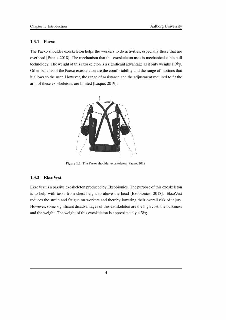
1.3.1 Paexo
The Paexo shoulder exoskeleton helps the workers to do activities, especially those that are
overhead [Paexo, 2018]. The mechanism that this exoskeleton uses is mechanical cable pull
technology. The weight of this exoskeleton is a significant advantage as it only weighs 1.9kg.
Other benefits of the Paexo exoskeleton are the comfortability and the range of motions that
it allows to the user. However, the range of assistance and the adjustment required to fit the
arm of these exoskeletons are limited [Luque, 2019].
Figure 1.3: The Paexo shoulder exoskeleton [Paexo, 2018]
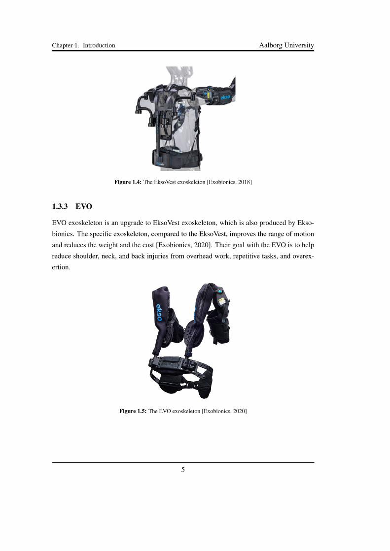
1.3.2 EksoVest
EksoVest is a passive exoskeleton produced by Eksobionics. The purpose of this exoskeleton
is to help with tasks from chest height to above the head [Exobionics, 2018]. EksoVest
reduces the strain and fatigue on workers and thereby lowering their overall risk of injury.
However, some significant disadvantages of this exoskeleton are the high cost, the bulkiness
and the weight. The weight of this exoskeleton is approximately 4.3kg.
4
Chapter 1. Introduction Aalborg University
Figure 1.4: The EksoVest exoskeleton [Exobionics, 2018]
1.3.3 EVO
EVO exoskeleton is an upgrade to EksoVest exoskeleton, which is also produced by Ekso-
bionics. The specific exoskeleton, compared to the EksoVest, improves the range of motion
and reduces the weight and the cost [Exobionics, 2020]. Their goal with the EVO is to help
reduce shoulder, neck, and back injuries from overhead work, repetitive tasks, and overex-
ertion.
Figure 1.5: The EVO exoskeleton [Exobionics, 2020]
5
Chapter 1. Introduction Aalborg University
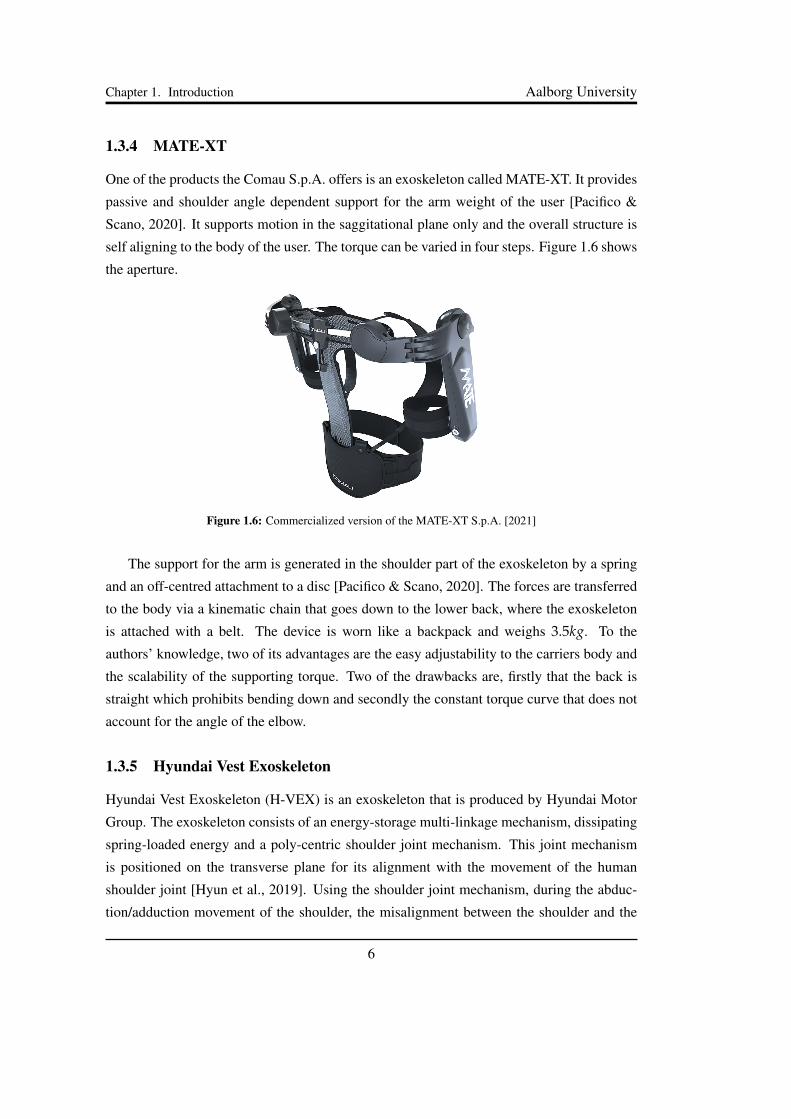
1.3.4 MATE-XT
One of the products the Comau S.p.A. offers is an exoskeleton called MATE-XT. It provides
passive and shoulder angle dependent support for the arm weight of the user [Pacifico &
Scano, 2020]. It supports motion in the saggitational plane only and the overall structure is
self aligning to the body of the user. The torque can be varied in four steps. Figure 1.6 shows
the aperture.
Figure 1.6: Commercialized version of the MATE-XT S.p.A. [2021]
The support for the arm is generated in the shoulder part of the exoskeleton by a spring
and an off-centred attachment to a disc [Pacifico & Scano, 2020]. The forces are transferred
to the body via a kinematic chain that goes down to the lower back, where the exoskeleton
is attached with a belt. The device is worn like a backpack and weighs 3.5kg. To the
authors’ knowledge, two of its advantages are the easy adjustability to the carriers body and
the scalability of the supporting torque. Two of the drawbacks are, firstly that the back is
straight which prohibits bending down and secondly the constant torque curve that does not
account for the angle of the elbow.
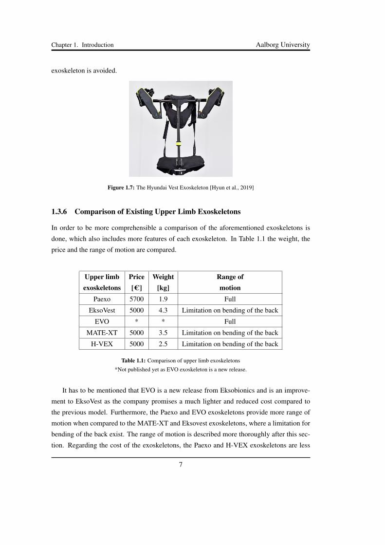
1.3.5 Hyundai Vest Exoskeleton
Hyundai Vest Exoskeleton (H-VEX) is an exoskeleton that is produced by Hyundai Motor
Group. The exoskeleton consists of an energy-storage multi-linkage mechanism, dissipating
spring-loaded energy and a poly-centric shoulder joint mechanism. This joint mechanism
is positioned on the transverse plane for its alignment with the movement of the human
shoulder joint [Hyun et al., 2019]. Using the shoulder joint mechanism, during the abduc-
tion/adduction movement of the shoulder, the misalignment between the shoulder and the
6
Chapter 1. Introduction Aalborg University
exoskeleton is avoided.
Figure 1.7: The Hyundai Vest Exoskeleton [Hyun et al., 2019]
1.3.6 Comparison of Existing Upper Limb Exoskeletons
In order to be more comprehensible a comparison of the aforementioned exoskeletons is
done, which also includes more features of each exoskeleton. In Table 1.1 the weight, the
price and the range of motion are compared.
Upper limbexoskeletons
Price[C]
Weight[kg]
Range ofmotion
Paexo 5700 1.9 Full
EksoVest 5000 4.3 Limitation on bending of the back
EVO * * Full
MATE-XT 5000 3.5 Limitation on bending of the back
H-VEX 5000 2.5 Limitation on bending of the back
Table 1.1: Comparison of upper limb exoskeletons
*Not published yet as EVO exoskeleton is a new release.
It has to be mentioned that EVO is a new release from Eksobionics and is an improve-
ment to EksoVest as the company promises a much lighter and reduced cost compared to
the previous model. Furthermore, the Paexo and EVO exoskeletons provide more range of
motion when compared to the MATE-XT and Eksovest exoskeletons, where a limitation for
bending of the back exist. The range of motion is described more thoroughly after this sec-
tion. Regarding the cost of the exoskeletons, the Paexo and H-VEX exoskeletons are less
7
Chapter 1. Introduction Aalborg University
expensive than the others.
1.4 Background of Existing Shoulder Joint Mechanisms
Different mechanisms are used in the shoulder to allow the exoskeleton to copy the motion
of the complex human shoulder joint. The mechanism used in traditional exoskeletons uses
a serial linkage, which consists of 3 revolute joints (3R) to implement the spherical motion
of the human shoulder joint [Christensen & Bai, 2017]. However, the mechanism collided
with the human body during the abduction motion. To overcome this drawback new designs
were developed. Some examples of mechanisms invented by AAU university are the Double
Parallelogram Linkage (DPL) [Christensen & Bai, 2017] and the Compact 3-DOF Scissors
Shoulder mechanism (SSM) [Castro et al., 2019] which are described in detail in this section.
Also, the mechanism used by H-VEX is described. At the end of this section, other existing
mechanisms are discussed briefly.
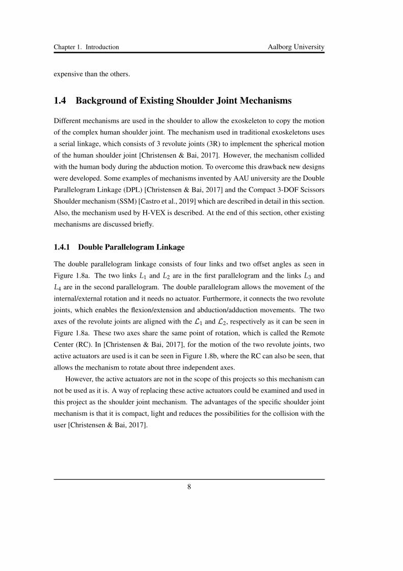
1.4.1 Double Parallelogram Linkage
The double parallelogram linkage consists of four links and two offset angles as seen in
Figure 1.8a. The two links L1 and L2 are in the first parallelogram and the links L3 and
L4 are in the second parallelogram. The double parallelogram allows the movement of the
internal/external rotation and it needs no actuator. Furthermore, it connects the two revolute
joints, which enables the flexion/extension and abduction/adduction movements. The two
axes of the revolute joints are aligned with the L1 and L2, respectively as it can be seen in
Figure 1.8a. These two axes share the same point of rotation, which is called the Remote
Center (RC). In [Christensen & Bai, 2017], for the motion of the two revolute joints, two
active actuators are used is it can be seen in Figure 1.8b, where the RC can also be seen, that
allows the mechanism to rotate about three independent axes.
However, the active actuators are not in the scope of this projects so this mechanism can
not be used as it is. A way of replacing these active actuators could be examined and used in
this project as the shoulder joint mechanism. The advantages of the specific shoulder joint
mechanism is that it is compact, light and reduces the possibilities for the collision with the
user [Christensen & Bai, 2017].
8
Chapter 1. Introduction Aalborg University
(a)
Axis-1
Axis-2
Axis-3Remote center
(b)
Figure 1.8: The double parallelogram linkage in a) and in b) the double parallelogram mechanism with the
active actuators for the two revolute joints [Christensen & Bai, 2017]
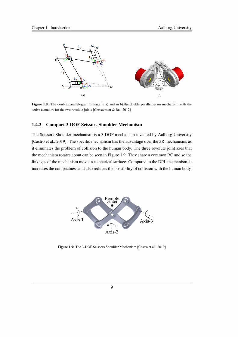
1.4.2 Compact 3-DOF Scissors Shoulder Mechanism
The Scissors Shoulder mechanism is a 3-DOF mechanism invented by Aalborg University
[Castro et al., 2019]. The specific mechanism has the advantage over the 3R mechanisms as
it eliminates the problem of collision to the human body. The three revolute joint axes that
the mechanism rotates about can be seen in Figure 1.9. They share a common RC and so the
linkages of the mechanism move in a spherical surface. Compared to the DPL mechanism, it
increases the compactness and also reduces the possibility of collision with the human body.
Axis-1
Axis-2
Remotecenter
Axis-3
Figure 1.9: The 3-DOF Scissors Shoulder Mechanism [Castro et al., 2019]
9

Chapter 1. Introduction Aalborg University
1.4.3 Four-bar Based Poly-Centric Shoulder Linkage
The four-bar based poly-centric shoulder linkage is used in the H-VEX as described be-
fore and can be seen in Figure 1.10. Other exoskeletons such as MATE and Eskovest, as
described before, use a redundant DOF around the scapula to overcome the misalignment
issue of the exoskeleton and the shoulder arm [Hyun et al., 2019]. In contrast, using the four-
bar based poly-centric shoulder linkage, no redundant DOF is needed and so the weight of
the exoskeleton is not increased unnecessarily. In the figure below the end point of the
poly-centric structure, P0, is in contact with the upper arm.
Figure 1.10: Anatomical shoulder structure with the four-bar based poly-centric structure (blue lines) on the
transverse plane [Hyun et al., 2019]
1.4.4 Other Existing Shoulder Joint Mechanisms
As mentioned before, conventional exoskeletons are using the serial linkage system with 3
revolute (3R) joints [Christensen & Bai, 2017], [Naidu et al., 2011]. The configuration of this
shoulder joint mechanism can be seen in Figure 1.11. The disadvantage of this configuration
is that it reduces the movement of the user in the coronal plane as it can collide with the
body.
10

Chapter 1. Introduction Aalborg University
Figure 1.11: The serial linkage with 3 revolute joints [Naidu et al., 2011]
Another shoulder joint mechanism can be seen in Figure 1.12. This shoulder joint mech-
anism overcomes the issue with the collision of the exoskeleton with the user’s body because
a circular guide is used in the arm. However, the drawback of this shoulder joint mechanism
is the singularity that can be seen in Figure 1.12 below, as there is an alignment of the axes
of rotations of the joints 1 and 3, respectively. This means that the exoskeleton can not pro-
duce the abduction movement in the transverse plane. Furthermore, the circular guide can
increase the weight of the exoskeleton by a significant amount.
Figure 1.12: The shoulder joint mechanism with two revolute joints and one circular guide [Lo & Xie, 2014]
One way of avoiding the singularity of the above shoulder joint mechanism is by intro-
ducing a redundant joint as can be seen in Figure 1.13. However, the issue with the weight
11

Chapter 1. Introduction Aalborg University
of the circular guide still exists. Besides the circular guide, the weight of the exoskeleton is
also increased as a redundant joint is added. This increases the workspace, but also makes
the exoskeleton bulkier.
Figure 1.13: The shoulder joint mechanism with three revolute joints and one circular guide [Lo & Xie, 2014]
1.5 Problem Formulation
Tasks as lifting, carrying or handling objects at work often result in musculoskeletal injuries,
such as strains and sprains [Exobionics, 2018]. Exoskeletons can be worn by employees in
the workplace to reduce the possibility of an injury. Although the existing passive upper limb
exoskeletons described before have significant advantages, their drawbacks are considerable
and should be improved.
The purpose of this project is to design a mechanism with one or more compliant ele-
ments, which will combine portability, modularity, and compactness. The compliant mech-
anism has to compensate for the gravitational forces and thereby reduce the risk of injuries.
Most of the exoskeletons presented above focus on flexion-extension movement, which
concerns mostly the workers on how to lift heavyweights. However, this is not the only
movement that can cause injuries and so also a concept for assistance in other planes should
be presented. This means that the designed exoskeleton ideally should assist the user in
movements in different planes than the sagittal plane, or should easily be upgradable. In
summary, the problem is formulated as:
12
Chapter 1. Introduction Aalborg University
A passive, compact and lightweight exoskeleton is to be developed, that supports the hu-
man arm movement by reducing the load acting on the shoulder muscles. Motion in the
sagittal plane is of highest priority, but differing planes also have to be considered. If possi-
ble with the Covid situation at hand, a prototype is to be used to validate the design. If this
proves impossible, numerical simulations are to be used for verification.
1.6 Problem Approach
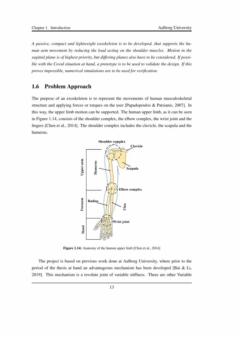
The purpose of an exoskeleton is to represent the movements of human musculoskeletal
structure and applying forces or torques on the user [Papadopoulos & Patsianis, 2007]. In
this way, the upper limb motion can be supported. The human upper limb, as it can be seen
in Figure 1.14, consists of the shoulder complex, the elbow complex, the wrist joint and the
fingers [Chen et al., 2014]. The shoulder complex includes the clavicle, the scapula and the
humerus.
Figure 1.14: Anatomy of the human upper limb [Chen et al., 2014]
The project is based on previous work done at Aalborg University, where prior to the
period of the thesis at hand an advantageous mechanism has been developed [Bai & Li,
2019]. This mechanism is a revolute joint of variable stiffness. There are other Variable
13
Chapter 1. Introduction Aalborg University
Stiffness Mechanisms (VSM), but to the authors best knowledge, their range of motion is
either too small to be used as torque providing device for an exoskeleton for the upper
limb [Dežman & Gams, 2018] [Wolf et al., 2011] [Jafari et al., 2010] [Wolf & Hirzinger,
2008], or their working principle is similar to the VSM developed at AAU [Furnémont et al.,
2015] [Vanderborght et al., 2009] [Van Ham et al., 2007]. This VSM is designed with a
compliant joint mechanism and is able to adjust the stiffness to the user’s needs by choosing
certain design parameters. However, the specific mechanism uses an external power to in- or
decrease the torque which makes it a pseudo-passive mechanism. To make it purely passive,
it will be reconfigured to be used without external power.
The shoulder joint mechanisms presented in Section 1.4 represent different solutions to
the problem of connecting an arm to the torso. All of those mechanisms provide different
advantages and disadvantages. Since the focus of this thesis is among others on compactness,
the SSM will be used. By providing three rotational DOF it follows the anatomical shoulder
closely and although other mechanisms, i.e. the four-bar based poly-centric shoulder linkage
used in the H-VEX exoskeleton, show better resemblance of certain motions of the shoulder
complex, the SSM is very compact and does not require additional structure to follow the
human body. The SSM, if physically realised, does not have singularities or redundant DOF,
which makes it attractive for this project.
First, the shoulder will be reduced to one rotational DOF, which can move in the sagittal
plane only and thereby capture the flexion-extension movement. The torque produced in
this 1-DOF system will be compared with the torque produced by the mechanism, whose
design concept will be analysed thoroughly in Chapter 2. After adjusting the parameters of
the VSM to obtain a torque profile that matches the shoulder torque profile, the exoskeleton
will be designed in detail and tested. Suggestions for additional design ideas are presented.
The exoskeleton will be assessed based on the experiments and general improvements will
be described.
14
Chapter 2
Modeling of the Exoskeleton
The following chapter explains the VSM as proposed by [Bai & Li, 2019] and [Li et al.,
2020]. Special focus is put on the kinematics and the rotation-torque relation. Furthermore,
the selected shoulder joint mechanism, which is the SSM, is described and analysed.
2.1 VSM Modeling
The following description is a short description of the VSM as described in [Bai & Li, 2019]
with the purpose of clarifying the following chapters. This section is based on [Bai & Li,
2019]. The torque that the VSM can provide can be utilized to compensate the gravitational
forces.
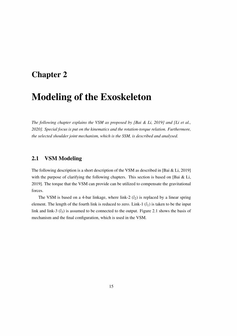
The VSM is based on a 4-bar linkage, where link-2 (l2) is replaced by a linear spring
element. The length of the fourth link is reduced to zero. Link-1 (l1) is taken to be the input
link and link-3 (l3) is assumed to be connected to the output. Figure 2.1 shows the basis of
mechanism and the final configuration, which is used in the VSM.
15
Chapter 2. Modeling of the Exoskeleton Aalborg University
3
2
1 θ1
2
3
4
1
32
θ
Figure 2.1: The initial four-bar linkage (left), which is the basis for the VSM. For the VSM the fourth link has
zero length and the bar-2 is a linear elastic element (center). On the right is the final configuration of the VSM.
The torque T of the three-bar linkage is given by the multiplication of the Jacobian of
the second link and the force produced by the spring:
T = JF (2.1)
where F is the tension force within the compliant coupler link-2.
With link-4 having no length, the length of bar two is expressed as
l2 =√
l21 + l2
3 − 2l1l3 cos θ (2.2)
where θ is the angle between the input and output links. For the VSM, the length l2 is
defining the Jacobian:
J =dl2dθ
(2.3)
The cable force F is composed of the force F0 due to pretension and the force due to elonga-
tion of the second link, δl2.
F = kδl2 + F0 (2.4)
where k is the stiffness of the spring.
By combining the equations and splitting them up into two terms, one influenced by
the stiffness of the elastic element and the other by the pretension , the following torque
expression is obtained:
T = kδl2 J + NF0 J (2.5)
However, the final configuration of the VSM, which is shown in Figure 2.1 on the right,
is composed of an inner (dashed light grey arc) and an outer (dashed dark grey arc) disc
with freely rotating pulleys (blue circles), connected by a cable. This is not exactly the same
configuration as the original three-bar linkage. Therefore the torque of the final configuration
changes. The torque provided from the final configuration of VSM is given as:
T = J1F = J1kδl + J1F0 (2.6)
16
Chapter 2. Modeling of the Exoskeleton Aalborg University
where δl is the elongation of the spring, J1 the Jacobian of the mechanism. They are defined
as:
δl = cNδl2 (2.7)
J1 = cNJ (2.8)
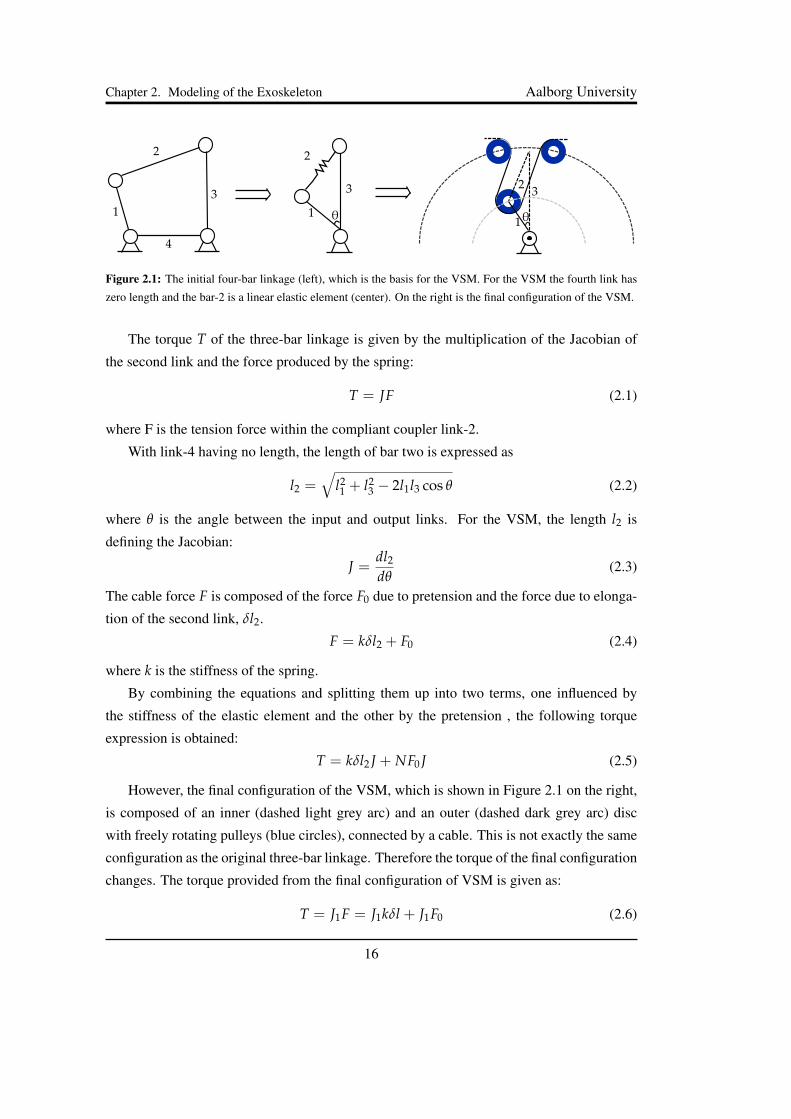
where c is a geometrical variable and N is the configuration number and is given by N =
1, 2, 3. The configuration number is the number of pulleys on the inner disc, that is connected
to the outer disc. For N = 1 the configuration is shown in Figure 2.1 whereas Figure 2.2
displays the arrangement for N = 2. For each connected pulley on the inner disc, two
pulleys of the outer disc have to be connected.
Figure 2.2: VSM configuration for N=2
From Equation (2.6) it can be concluded that the torque of the configuration, besides the
length of the links and the spring properties, is also depended on the configuration number
N and the geometrical variable c. The value for the geometric value is taken equal to 2, the
reason for this is explained in Appendix A.
Figure 2.3 shows a torque curve of a VSM with arbitrary values for the design parame-
ters.
17

Chapter 2. Modeling of the Exoskeleton Aalborg University
Figure 2.3: Torque over relative angle θ for k = 4, F0 = 0, N = 1
2.2 AAU’s Scissors Shoulder Mechanism
In a PhD thesis presented at Aalborg University, a novel shoulder joint mechanism has been
suggested. To allow for all rotatory degrees of freedom of a human shoulder, the links of
the mechanism lay on a sphere, which has its centre in the centre of rotation of the shoulder
[Castro et al., 2019]. To eliminate singularities that result from locking of motions in certain
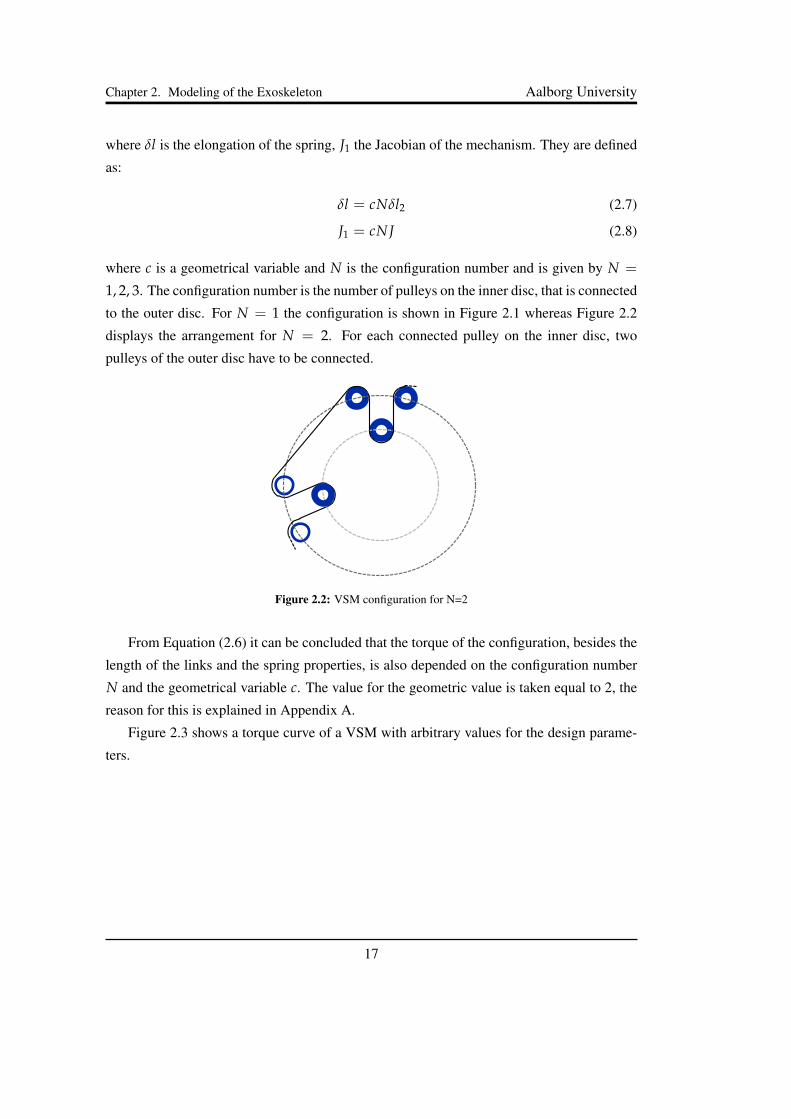
configurations, the SSM is composed of a row of two parallelograms as shown in Figure 2.4.
This avoids the singularities and enables the same range of motion as provided by the human
shoulder. As it can be seen in the figure below, the SSM consists of six linkages - four short
and two long ones. The small linkages, which have half of the length of the longer ones, are
connected with each other and the bigger one via a revolute joint. The two bigger linkages,
which are located in the middle of the SSM, are also connected with a revolute joint in their
centre point.
18
Chapter 2. Modeling of the Exoskeleton Aalborg University
Figure 2.4: The SSM prototype [Castro et al., 2019]
2.2.1 Kinematics of the SSM
In order to describe the motion of the SSM, the kinematics of it has to be analysed. This can
be done through forward kinematics or inverse kinematics. In the first analysis, the position
of the end-effector is found with the angle of the joints given. In contrast, using inverse
kinematics, the angles of the joints are found based on the location of the end-effector. For
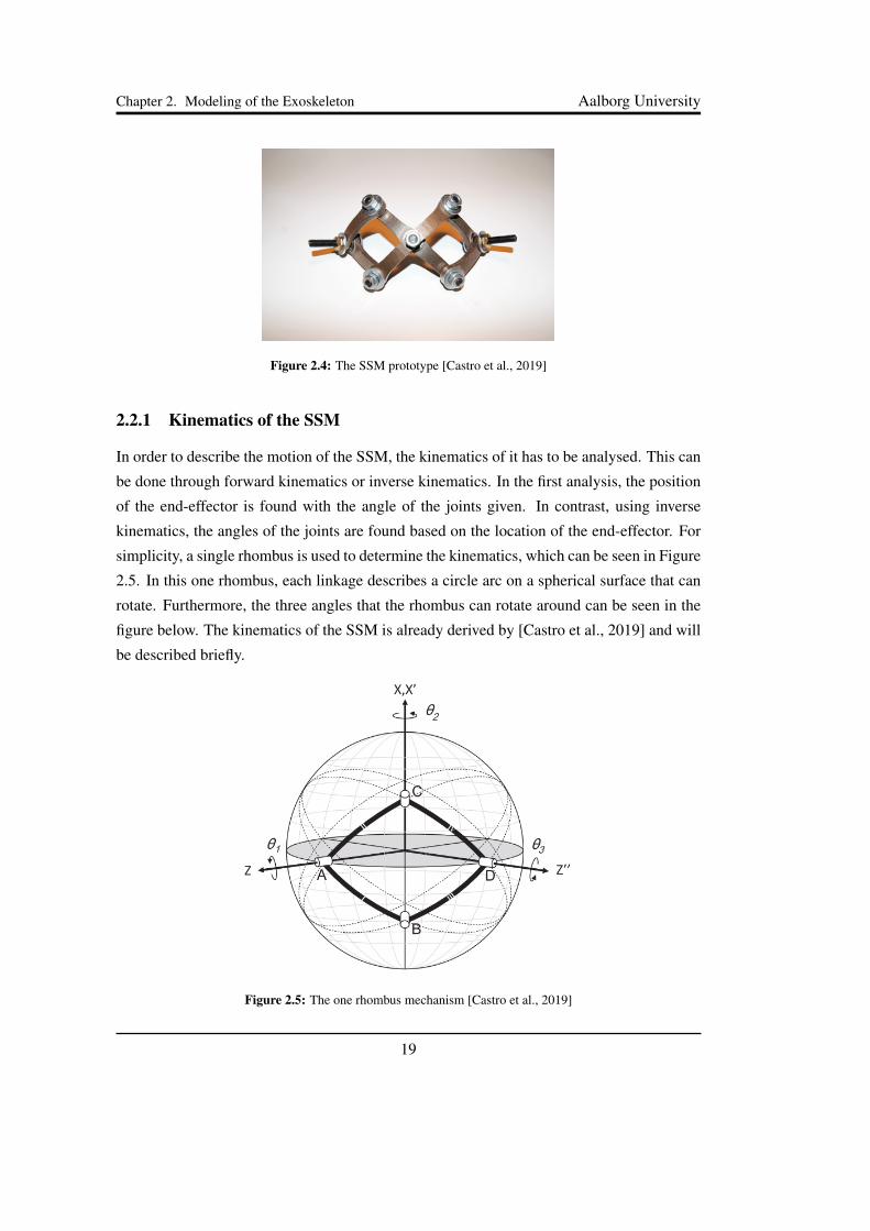
simplicity, a single rhombus is used to determine the kinematics, which can be seen in Figure
2.5. In this one rhombus, each linkage describes a circle arc on a spherical surface that can
rotate. Furthermore, the three angles that the rhombus can rotate around can be seen in the
figure below. The kinematics of the SSM is already derived by [Castro et al., 2019] and will
be described briefly.
Figure 2.5: The one rhombus mechanism [Castro et al., 2019]
19

Chapter 2. Modeling of the Exoskeleton Aalborg University
Forward Kinematics
For the forward kinematics, the inter-linkage angles ϕi and the Euler angles θi are used to
find the rotation matrix Re. The rotation matrix refers to the transformation of the end-
effector coordinates to the ones of the global frame. For all the frames, the remote centre
that was shown in Figure 1.9, is chosen. In Figure 2.6, where the different angles are shown,
it can also be seen that there is an extra link VI, which represents the end-effector.
Figure 2.6: Inter-linkage joint angles ϕi and the Euler angles θi in the SSM [Castro et al., 2019]
From the figure above the equations that can be derived are:
θ1 = ϕ1 +ϕ1
2(2.9)
θ3 = ϕ6 −ϕ2
2(2.10)
Another equation can be derived using the spherical law of cosines:
cos θ2 = cos2 α + sin2 α cos(π − ϕ2)⇒ θ2 = arccos(cos2 α− sin2 α cos ϕ2) (2.11)
Equation (2.11) describes the relation between the end-effector pitch angle θ2 and the in-
ternal angle ϕ2. This relation is represented in Figure 2.7 for different values of the curvature
angle α.
20

Chapter 2. Modeling of the Exoskeleton Aalborg University
Figure 2.7: The relation between the end-effector pitch angle θ2 and the internal angle φ2 for different values
of the curvature angle α
From the figure above it can be seen that when the curvature angle α is increased, the
end-effector pitch angle θ2 is increased. Furthermore, for ϕ2 = 0, the end-effector pitch
angle θ2 is twice the curvature angle α.
In order to relate the end-effector with the global reference frame the rotation matrices
Rz(θ1), Rx(θ2) and Rz(θ3) are used. These matrices express the ’route’ from the end
effector to the point A. The three rotations matrices are found as:
Rz(θ1) =
cθ1 −sθ1 0
sθ1 cθ1 0
0 0 1
(2.12)
Rx(θ2) =
1 0 0
0 cθ2 −sθ2
0 sθ2 cθ2
(2.13)
Rz(θ3) =
cθ3 −sθ3 0
sθ3 cθ3 0
0 0 1
(2.14)
With the three rotation matrices, and since all the links have as a common origin the
remote centre as shown in Figure 1.9, the rotation matrix Re is found as:
21

Chapter 2. Modeling of the Exoskeleton Aalborg University
Re = Rz(θ1)Rx(θ2)Rz(θ3) =
cθ1cθ3 − sθ1cθ2sθ3 −cθ1sθ3 − sθ1cθ2cθ3 sθ1sθ2
sθ1cθ3 + cθ1cθ2sθ3 −sθ1sθ3 − cθ1cθ2cθ3 −cθ1sθ2
sθ2sθ3 sθ2cθ3 cθ2
(2.15)
where sθi and cθi correspond to the sine and cosine functions of the angle θ.
Assuming a sphere of 60mm radius three cases of the position of the end-effector with
respect to an initial point, which is located in the position z = 60mm, x = 0mm, z′ = 0mm,
can be seen in Figure 2.8. The Case 1 is for θ1 = 0◦, θ2 = 45◦, θ3 = 0◦, Case 2 is for
θ1 = 90◦, θ2 = 135◦, θ3 = 0◦ and Case 3 for θ1 = 45◦, θ2 = 90◦, θ3 = 0◦.
Figure 2.8: End effector position for three different cases depending on the pitch angles θ1, θ2, θ3
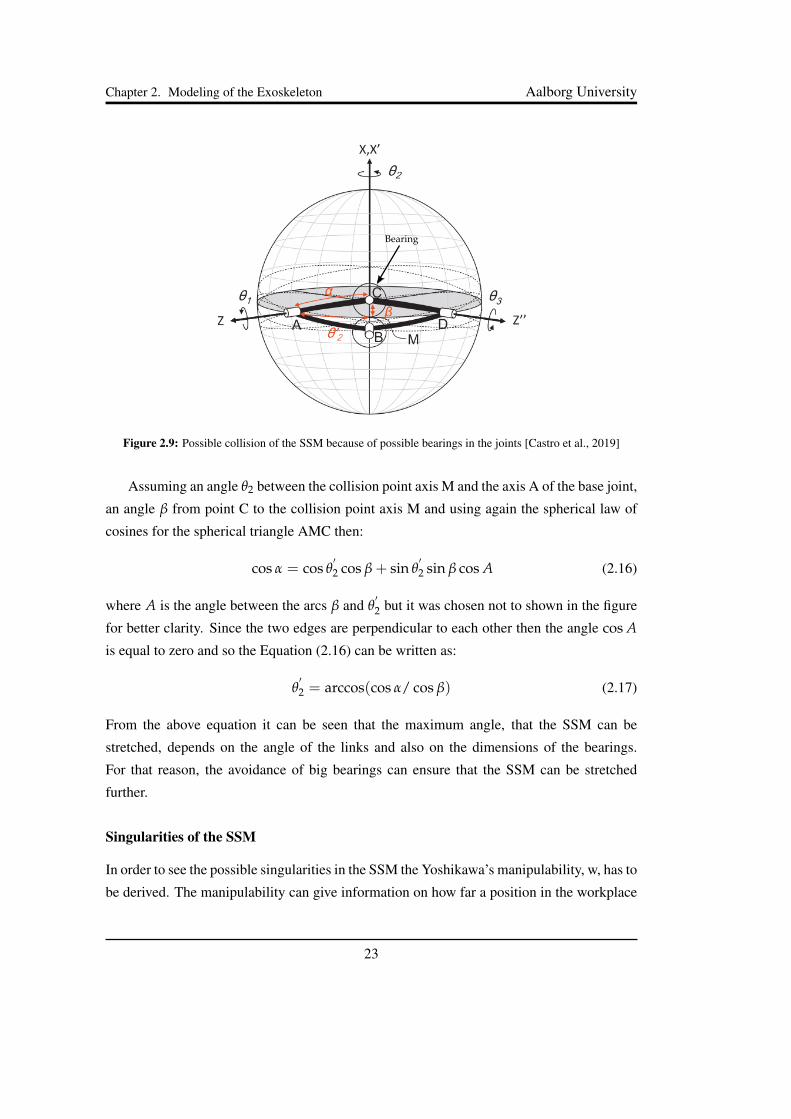
2.2.2 Design Limitations
A limitation of the SSM prototype is the collision of the bearings as can be seen in Figure
2.9. This happens when the SSM are fully stretched or fully folded.
22
Chapter 2. Modeling of the Exoskeleton Aalborg University
Bearing
Figure 2.9: Possible collision of the SSM because of possible bearings in the joints [Castro et al., 2019]
Assuming an angle θ2 between the collision point axis M and the axis A of the base joint,
an angle β from point C to the collision point axis M and using again the spherical law of
cosines for the spherical triangle AMC then:
cos α = cos θ′2 cos β + sin θ
′2 sin β cos A (2.16)
where A is the angle between the arcs β and θ′2 but it was chosen not to shown in the figure
for better clarity. Since the two edges are perpendicular to each other then the angle cos Ais equal to zero and so the Equation (2.16) can be written as:
θ′2 = arccos(cos α/ cos β) (2.17)
From the above equation it can be seen that the maximum angle, that the SSM can be
stretched, depends on the angle of the links and also on the dimensions of the bearings.
For that reason, the avoidance of big bearings can ensure that the SSM can be stretched
further.
Singularities of the SSM
In order to see the possible singularities in the SSM the Yoshikawa’s manipulability, w, has to
be derived. The manipulability can give information on how far a position in the workplace
23
Chapter 2. Modeling of the Exoskeleton Aalborg University
is from a singularity [Vahrenkamp et al., 2012]. It is defined relative to the determinant of
the Jacobian J as:
w =√
det (J JT) (2.18)
The Jacobian matrix is found from the equation that relates the angular velocities ωe with
the mechanism’s joint velocities θ and is equal to:
J =
0 cθ1 sθ1sθ2
0 sθ1 −cθ1sθ2
1 0 cθ2
(2.19)
More details on how the Jacobian is derived can be found in Appendix B.
Substituting Equation (2.19) into Equation (2.18), the manipulability is equal to:
w =| sθ2 | (2.20)
From the above equation it can be seen that the manipulability and so the possible singular-
ities depend on the pitch angle θ2. For the singularities to appear, the manipulability has to
be equal to zero. This happens in two cases:
w =
0, θ2 = 0◦ ⇔ φ2 = 180◦
0, θ2 = 180◦ ⇔ φ2 = 0◦(2.21)
From the above equations it can be concluded that the first singularity happens when the
SSM is totally closed (θ2 = 0◦), which automatically means that the joint angle φ2 = 180◦.
The second singularity occurs when the SSM is fully stretched (θ2 = 180◦), which results
in the joint angle φ2 = 0◦. From Figure 2.7 it can be seen that this situation occurs when
α = 90◦. The two relations can also be verified from equation (2.11).
According to [Castro et al., 2019], the first singularity happens at 90◦ of shoulder ex-
ternal rotation and the second one at 90◦ of internal rotation. Both singularities should not
concern the user as the first one is unusual in daily activity and the second one cannot exist
because it would mean the penetration of the torso.
However, to avoid or come close to these two singularities a relation was derived in
[Castro et al., 2019], in which the θ2max is dependent on the number of rhombus n and the
linkage curvature angle α as:
θ2max = 2αn < 180◦ (2.22)
24
Chapter 2. Modeling of the Exoskeleton Aalborg University
As mentioned before, the holes of the links are surrounded by material in order to include
the bearings, bolts etc. This means that the possible singularities described before will not
happen as θ2 or ϕ2 can not reach the 0◦ and 180◦. Combining Equation (2.17) and Equation
(2.22) the limits of θ2 can be derived as:
θ2max = 2nθ′2 (2.23)
θ2min = 2nβ (2.24)
Having these two equations, stability of the mechanism is achieved since the singularities
are avoided as it ensures that the pitch angle θ2 can not reach the singularity angles 0◦ and
180◦.
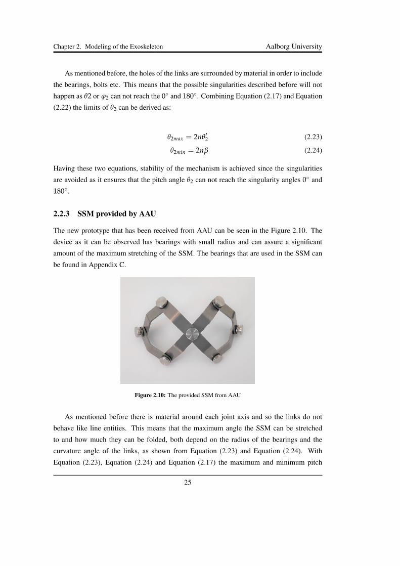
2.2.3 SSM provided by AAU
The new prototype that has been received from AAU can be seen in the Figure 2.10. The
device as it can be observed has bearings with small radius and can assure a significant
amount of the maximum stretching of the SSM. The bearings that are used in the SSM can
be found in Appendix C.
Figure 2.10: The provided SSM from AAU
As mentioned before there is material around each joint axis and so the links do not
behave like line entities. This means that the maximum angle the SSM can be stretched
to and how much they can be folded, both depend on the radius of the bearings and the
curvature angle of the links, as shown from Equation (2.23) and Equation (2.24). With
Equation (2.23), Equation (2.24) and Equation (2.17) the maximum and minimum pitch
25

Chapter 2. Modeling of the Exoskeleton Aalborg University
angles for θ2 can be found. The results of the pitch angles and the specifications of the new
SSM prototype can be seen in Table 2.1.
Linkage curvature angle α 38◦
Intruisive angle β 3◦
θ2max 151.5◦
θ2min 12◦
Table 2.1: Specifications of the provided SSM and the maximum and minimum pitch angles
From the above table the limits of θ2 can be seen. It can be concluded that the SSM
allows 78◦ of external shoulder rotation and 61.5◦ of internal shoulder rotation.
26

Chapter 3
Assistance in the Sagittal Plane
In the following chapter, a model for the motion of a human arm in the sagittal plane is
presented. Based on this kinematic model optimisation is used to adjust the parameters of a
VSM to obtain a best possible support for the important ranges of motion.
3.1 Motion of the Human Arm
To model the human arm, three sections are considered: the upper arm, the forearm and the
hand. Those sections are connected by joints of various degrees of freedom. The shoulder
joint or glenohumeral joint is a ball and socket joint. Following Reference [Zhang et al.,
2011] it is kinematically represented by a spherical joint, resembled by three revolute joints,
which have zero distance between each other and whiches axes of rotation are perpendicular
to each other. The elbow can conduct two rotations, one that rotates the forearm around itself
and one perpendicular to both the forearm and the upper arm. Thus it can be represented by
two revolute joints with zero distance from each other. The wrist joint is included as a ball
and socket joint with two rotational degrees of freedom [Soames et al., 1994]. In total, the
model of the arm has seven degrees of freedom. To determine the position of the joints and
the centres of mass of the different segments in space, the rotation matrices for the different
coordinate systems of the joints are introduced in the following. The general coordinate sys-
tem of the reference frame with index m is thereby oriented such that the x-axis is pointing
sideways away from the body, the y-axis is pointing towards the front and the y-axis is point-
ing upward. The origin of the reference frame is located in the centre of the glenohumeral
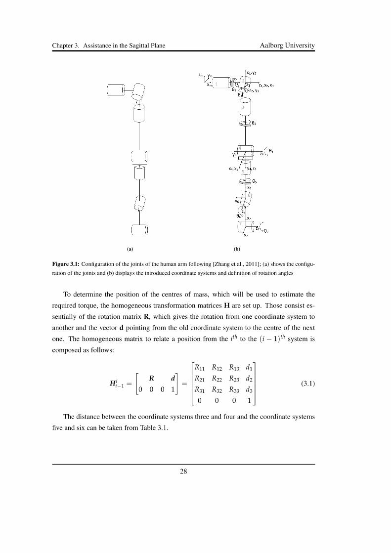
joint. In the following Figure 3.1 the arrangement of the joints is depicted along with the
introduced coordinate systems and the positive definition of the rotation angles.
27
Chapter 3. Assistance in the Sagittal Plane Aalborg University
(a) (b)
Figure 3.1: Configuration of the joints of the human arm following [Zhang et al., 2011]; (a) shows the configu-
ration of the joints and (b) displays the introduced coordinate systems and definition of rotation angles
To determine the position of the centres of mass, which will be used to estimate the
required torque, the homogeneous transformation matrices H are set up. Those consist es-
sentially of the rotation matrix R, which gives the rotation from one coordinate system to
another and the vector d pointing from the old coordinate system to the centre of the next
one. The homogeneous matrix to relate a position from the ith to the (i − 1)th system is
composed as follows:
H ii−1 =
[R d
0 0 0 1
]=
R11 R12 R13 d1
R21 R22 R23 d2
R31 R32 R33 d3
0 0 0 1
(3.1)
The distance between the coordinate systems three and four and the coordinate systems
five and six can be taken from Table 3.1.
28

Chapter 3. Assistance in the Sagittal Plane Aalborg University
SegmentLength
[mm]
Centre of Mass*
[%]
Weight**
[%]
Upper Arm 281.7 57.72 2.71
Forearm 268.9 45.74 1.62
Hand 86.2 79.00 0.61
Table 3.1: Dimensions for the male arm [de Leva, 1996]
* Distance from the joint in percent of the segment length
** in percent of the body weight
With the distances given the homogeneous matrices are set up and can be seen in Ap-
pendix D. The indexing is done in such a way that the lower index refers to the original
coordinate system and the upper one is the coordinate system that a point is related with. To
obtain a translation of a point from an arbitrary coordinate system n to the base frame, the
homogeneous matrices are multiplied.
Hnm = H1
mH21 H3
2 ...Hnn−1 (3.2)
Thus the position of the arm can now be described in the base coordinate system and if the
position of a point in one of the mentioned coordinate systems is known, it is also known in
relation to the body. Figure 3.2 shows the arm in about the position to grab a glass from a
table. The shoulder and elbow are both in flexion and the hand is held in hyperextension.
Figure 3.2: Arm model with θ1 = −45◦, θ4 = 45◦ and θ6 = 30◦; all other angles are zero. The shoulder,
elbow and wrist are marked with a red circle. The green circles indicate the position of the centre of mass of the
segments according to [de Leva, 1996]. The shoulder joint is positioned in the origin of the m-system.
29

Chapter 3. Assistance in the Sagittal Plane Aalborg University
For the estimation of the required torque to keep the arm elevated in a certain position
the lever arms of the centres of mass are of special interest. Those are calculated from the x-
and y-coordinates of the centres of mass of the different segments by use of the Pythagoras
theorem. The torque that is required to keep a segment elevated is the vector product of its
centre of mass and the individual force vector. The direction and magnitude of the torque
of the whole arm is then given by the vector sum of the torque vectors of the individual
segments.
3.2 Motion of a Human Arm in the Sagittal Plane
To develop an exoskeleton for the whole arm with seven actuators is out of the scope of
this work. Therefore the general model from the previous section is reduced to only two
actuators: θ1 and θ4. For simplification, those are renamed as follows:
θ1 = γ (3.3)
θ4 = α (3.4)
In this reduced model, the hand is not considered to move but stays aligned with the forearm.
In that case, pronation and supination have no influence on the position of the centre of
gravity in space, which is why they are not considered and the corresponding actuator 5
is fixed at θ5 = 0◦. Hence, the first degree of motion that is considered, is flexion of the
shoulder with the elbow angle α acting within the sagittal plane. This makes the overall
shoulder torque a function of two inputs and defines its direction to be perpendicular to the
sagittal plane. Figure 3.3 depicts the simplified arm model.
α
γ1
23
Figure 3.3: Graphical explanation of γ and α
30

Chapter 3. Assistance in the Sagittal Plane Aalborg University
The torque that is necessary to counter the gravitational forces for a sequence of n links
in 2D with point masses is given by
Tshoulder = gn
∑i=1
lCMimi (3.5)
where lCMi is the lever arm of the mass of the ith segment, mi is the mass of the segment and
g is the gravitational acceleration. The length lCMi is
lCMi =i−1
∑j=1
lj sinj
∑k=1
αk + cili sini
∑l=1
αl (3.6)
with αi being the angle between a link and its precursor. Applied to the n = 3 mechanism
at hand with no angle between the hand and the forearm the three lever arms become
lCM1 = c1l1 sin γ
lCM2 = l1 sin γ + c2l2 sin (γ + α)
lCM3 = l1 sin γ + l2 sin (γ + α) + c3l3 sin (γ + α + 0)
(3.7)
The weight of the segments is given from the person’s weight and Table 3.1. With the
mentioned considerations, the torque that the shoulder has to create can be calculated. Figure
3.4 shows the resulting curves.
Figure 3.4: Torque that is needed to counter the torque produced by the mass forces over the shoulder angle γ
for different elbow angels α
It is noted, that there is no payload taken into account. The main reason is, that a passive
exoskeleton is not capable of reacting to changes in the required torque by itself. Hence,
31
Chapter 3. Assistance in the Sagittal Plane Aalborg University
if the payload is considered wrongly to be too large, the positive effect of the support of
the exoskeleton may be turned into a negative one, when the user has to constantly apply a
downward torque instead of an upward torque to keep the arm at a constant level. This espe-
cially applies to the torque curves of α > 0◦ due to the sign change for large γ. The VSM as
considered in this thesis cannot sense this and will apply torque in the same direction as the
arm. Thus the human muscles are dealing with heavier loads than without the exoskeleton.
Contrary to this higher loading of the body, even too small assistance reduces the risk of
injuries [Maurice et al., 2020].
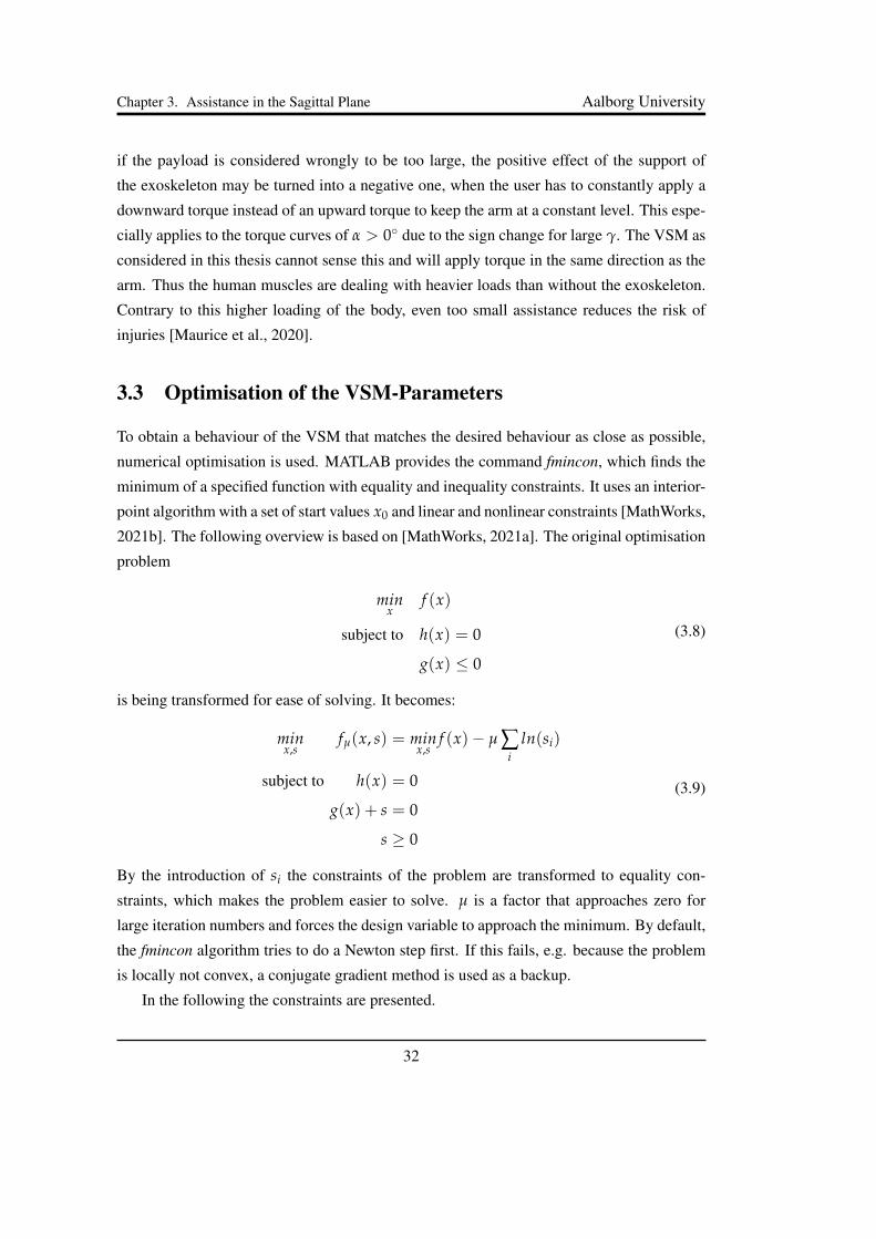
3.3 Optimisation of the VSM-Parameters
To obtain a behaviour of the VSM that matches the desired behaviour as close as possible,
numerical optimisation is used. MATLAB provides the command fmincon, which finds the
minimum of a specified function with equality and inequality constraints. It uses an interior-
point algorithm with a set of start values x0 and linear and nonlinear constraints [MathWorks,
2021b]. The following overview is based on [MathWorks, 2021a]. The original optimisation
problem
minx
f (x)
subject to h(x) = 0
g(x) ≤ 0
(3.8)
is being transformed for ease of solving. It becomes:
minx,s
fµ(x, s) = minx,s
f (x)− µ ∑i
ln(si)
subject to h(x) = 0
g(x) + s = 0
s ≥ 0
(3.9)
By the introduction of si the constraints of the problem are transformed to equality con-
straints, which makes the problem easier to solve. µ is a factor that approaches zero for
large iteration numbers and forces the design variable to approach the minimum. By default,
the fmincon algorithm tries to do a Newton step first. If this fails, e.g. because the problem
is locally not convex, a conjugate gradient method is used as a backup.
In the following the constraints are presented.
32

Chapter 3. Assistance in the Sagittal Plane Aalborg University
Constraints
• Dimension of l3To restrict l3 from getting larger than 60mm and smaller than the diameter of a pulley
and l1 the following constraint is established. A distance of 1mm is enforced between
the two pulleys and 3mm distance between the outer edge of the mechanism is defined.
l1 + 2R ≤ l3 ≤ 60mm− R− 3mm (3.10)
• Dimensions of l1The length l1 has to be restricted in a similar way to prevent it from becoming too
small. The relation between l1 and l3 is defined in Equation (3.10).
R + 3mm ≤ l1 (3.11)
• Constraint for spring stiffness
The stiffness of the spring has to be larger than 0Nmm and has no upper boundary.
0 ≤ k ≤ ∞ (3.12)
• Constraint for the pretension F0
The cable that connects the input and output shaft cannot handle negative pretensions,
therefore F0 has to be positive at all points. Material limits are not taken into account
at this point, so there is no upper boundary to the pretension.
0 ≤ F0 ≤ ∞ (3.13)
• Size constraint for the pulleys
The size of the pulleys must not get too large, hence the radius R is restricted:
6.5mm ≤ R ≤ 15mm (3.14)
• Length constraint of the spring
The overall length of the spring is restricted to fit between the shoulder joint and the
elbow. This space is further reduced, because of the dimensions of the VSM. The final
design of the VSM cannot be determined yet, but an estimate is
d = 2(l3 + R) + 60mm (3.15)
33

Chapter 3. Assistance in the Sagittal Plane Aalborg University
where an extra 60mm are added to account for design choices that might occur later.
The maximum spring elongation ∆lc occurs when the angle between l1 and l3 is 180◦,
which results in
∆lc = 2 · 2l1 (3.16)
Combined with the spring elongation due to the pretension and the length of the upper
arm as a maximum value from Table 3.1 the constraint is:
F0
k+ 4l1 ≤ 281.7− d
2(3.17)
Objective Function
Ideally, the VSM shows the same torque behaviour as the shoulder in reverse direction. With
the models for VSM and the shoulder torque in place, the basis for the objective function
is taken to be the difference between the required torque, which is the shoulder torque, and
the provided torque from the VSM. To have an effective torque of zero when the arm is at
γ = 0◦, the angle θ of the VSM has to be periods of 180◦. Since the VSM has to provide
energy, the stored potential energy has to be higher when the arm is hanging down than when
the arm is raised. Therefore if γ = 0◦, the internal angle of the VSM has to be θ = 180◦.
To obtain a more intuitive formulation of the objective function, it is made use of the point
symmetry of the torque curve of the VSM and θ is related to γ
θ = 180◦ − γ (3.18)
This results in a torque that is positive over the domain of the optimisation for the VSM
and the shoulder model, although the torque resulting from the mass forces of the arm is
of opposite sign than the torque of the VSM. In Equation (3.20) the deviation is hence a
subtraction.
To also minimize the required prior elongation of the spring, the ratio between F0 and
the spring stiffness k is added as the exponent of an e-function. Thereby a large penalty
is introduced if this ratio is large and configurations with small starting elongations l0 are
favoured. The error is squared to account for varying signs and cumulated over all elbow
angles α and shoulder angles γ:
f (x) =180◦
∑γ=0◦
150◦
∑α=0◦
(w · (Tshoulder − TVSM))2 + eF0k (3.19)
w is a weight function that is introduced to emphasize the influence of certain angles α and
γ that are considered more important than others.
34

Chapter 3. Assistance in the Sagittal Plane Aalborg University
Weight Function
The initial purpose of the exoskeleton is to ease overhead working tasks. For those the elbow
angle α is mostly between 10◦ and 90◦. The higher angles to the end of the considered range
are deemed less important and the maximum w.r.t. α is constructed at around 50◦. To lever-
age the importance of the shoulder angle γ that are around 110◦, a function that is quatratic
w.r.t. γ is included. The specific parameters are found with a MATLAB optimisation. The
weight function is
w(γ, α) =(
p1ep2(α+3)+p3 + p4ep5(α+3)+p6 + p7ep8(α+3)+p9 + p10e−α−3)
·(−0.0002 (γ− 110◦)2 + 3
) (3.20)
Parameter Value Parameter Value Parameter Value Parameter Value
p1 579.08 p4 -0.04 p7 763.92 p10 3.97
p2 -0.05 p5 0.23 p8 -0.03
p3 -1.72 p6 7.06 p9 0.32
Table 3.2: Parameters p1...10 of the weight function.
Table 3.2 contains the values of the parameters of the weight function. In Equation (3.20)
the function is offset of 3◦ to the negative α-direction. This is to avoid a shift in the gradient
at α = 0 in Equation (3.20). Figure 3.5 shows the graphs of the main terms of the weight
function. The complete weight function in the region of interest is depicted in Figure 3.6.
(a) (b)
Figure 3.5: Graphs of the components of the weight function, 3.5a shows the weight function at α = 0◦, 3.5b
shows the graph at γ = 0◦
35
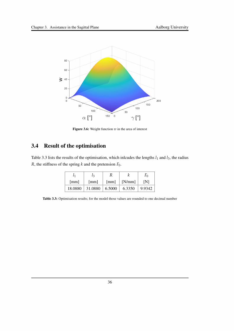
Chapter 3. Assistance in the Sagittal Plane Aalborg University
Figure 3.6: Weight function w in the area of interest
3.4 Result of the optimisation
Table 3.3 lists the results of the optimisation, which inlcudes the lengths l1 and l3, the radius
R, the stiffness of the spring k and the pretension F0.
l1[mm]
l3[mm]
R[mm]
k[N/mm]
F0
[N]
18.0880 31.0880 6.5000 6.3350 9.9342
Table 3.3: Optimisation results; for the model those values are rounded to one decimal number
36

Chapter 3. Assistance in the Sagittal Plane Aalborg University
Figure 3.7: Torque curves of the shoulder model, the VSM model and 50% of the VSM model for α =
0◦, 45◦, 90◦, 135◦; The curves have been adjusted to be in the same quadrant although they are of opposing
signs.
Figure 3.7 displays the curves of the shoulder model and the VSM model. It also includes
the graph of half the VSM torque. The signs of the curves have been adjusted to show them
all next to each other although the torque due to gravity is of opposite direction that the
torque of the mechanism. For the VSM to be effective, the angle θ has to be 180◦ when the
arm is hanging down, that is at γ = 0◦, so that the energy, that is stored in the spring, is able
to support the lifting process.
As can be seen from Figure 3.7, for a straight arm and shoulder angles up to around
60 degrees the VSM matches the required shoulder model very well. For higher shoulder
angles γ with straight elbow the VSM torque shows a constant difference to the shoulder
torque, but it follows the shape of the curve quite well. For elbow angles of α = 45◦ the
VSM matches the shoulder torque very well for shoulder angles between 80◦ and 170◦. This
is unsurprising, as the objective function was intentionally designed to fit this area best. The
cost of the good fit for α = 45◦ is, that with increasing elbow angles the VSM does not
match the shoulder torque very well. It shows some drawback for α = 90◦ and a significant
difference to the torque with α = 135◦. Those drawbacks are decreased significantly, if only
half the shoulder torque is compensated. This provides the advantage, that the user does
not need to put in extra effort to pull down the mechanism. This also reduces the expected
weight and size of the design. Hence, in this thesis 50% support are implemented.
37
Chapter 4
Conceptual Design and Numerical Val-idation of the VSM
In this chapter, the preliminary design of the VSM and the assembly of the exoskeleton is de-
scribed. Furthermore, a numerical analysis is carried out in order to validate the behaviour
of the designed VSM. The numerical simulation is performed in the software MSC ADAMS.
The analysis includes the maximum torque that the VSM can provide and also the angle that
this corresponds with. Results regarding the deformation of the spring are described. In
the end, a comparison of the numerical analysis with the analytical analysis described in
Chapter 3 is done.
4.1 Preliminary Design
The initial design of the exoskeleton is based on the dimensions that are obtained from
the optimisation and the selection of the extension spring. The exoskeleton is divided into
several different assemblies which are explained in detail in this section.
4.1.1 VSM Assembly
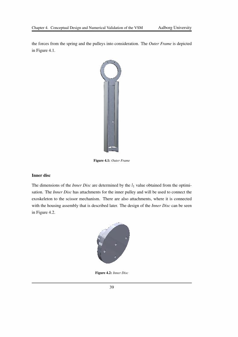
Outer Frame
The dimensions of the Outer Frame are determined by the l3 value obtained from the opti-
misation result and the dimensions of the selected spring. The Outer Frame has attachments
for the pulleys, spring and the cuff. The design of the frame is done with intuition, by taking
38
Chapter 4. Conceptual Design and Numerical Validation of the VSM Aalborg University
the forces from the spring and the pulleys into consideration. The Outer Frame is depicted
in Figure 4.1.
Figure 4.1: Outer Frame
Inner disc
The dimensions of the Inner Disc are determined by the l1 value obtained from the optimi-
sation. The Inner Disc has attachments for the inner pulley and will be used to connect the
exoskeleton to the scissor mechanism. There are also attachments, where it is connected
with the housing assembly that is described later. The design of the Inner Disc can be seen
in Figure 4.2.
Figure 4.2: Inner Disc
39
Chapter 4. Conceptual Design and Numerical Validation of the VSM Aalborg University
4.1.2 Scissors Assembly
SSM
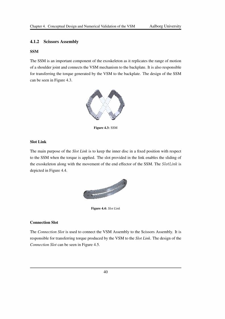
The SSM is an important component of the exoskeleton as it replicates the range of motion
of a shoulder joint and connects the VSM mechanism to the backplate. It is also responsible
for transferring the torque generated by the VSM to the backplate. The design of the SSM
can be seen in Figure 4.3.
Figure 4.3: SSM
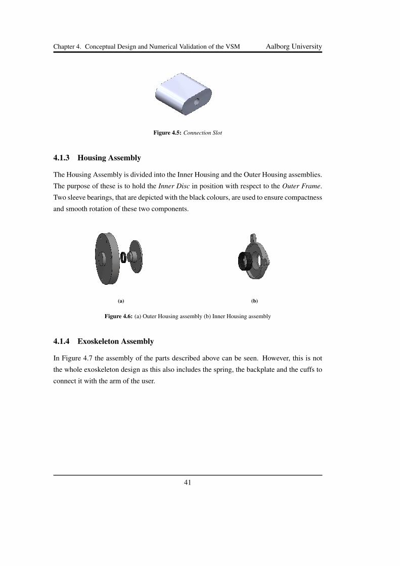
Slot Link
The main purpose of the Slot Link is to keep the inner disc in a fixed position with respect
to the SSM when the torque is applied. The slot provided in the link enables the sliding of
the exoskeleton along with the movement of the end effector of the SSM. The SlotLink is
depicted in Figure 4.4.
Figure 4.4: Slot Link
Connection Slot
The Connection Slot is used to connect the VSM Assembly to the Scissors Assembly. It is
responsible for transferring torque produced by the VSM to the Slot Link. The design of the
Connection Slot can be seen in Figure 4.5.
40
Chapter 4. Conceptual Design and Numerical Validation of the VSM Aalborg University
Figure 4.5: Connection Slot
4.1.3 Housing Assembly
The Housing Assembly is divided into the Inner Housing and the Outer Housing assemblies.
The purpose of these is to hold the Inner Disc in position with respect to the Outer Frame.
Two sleeve bearings, that are depicted with the black colours, are used to ensure compactness
and smooth rotation of these two components.
(a) (b)
Figure 4.6: (a) Outer Housing assembly (b) Inner Housing assembly
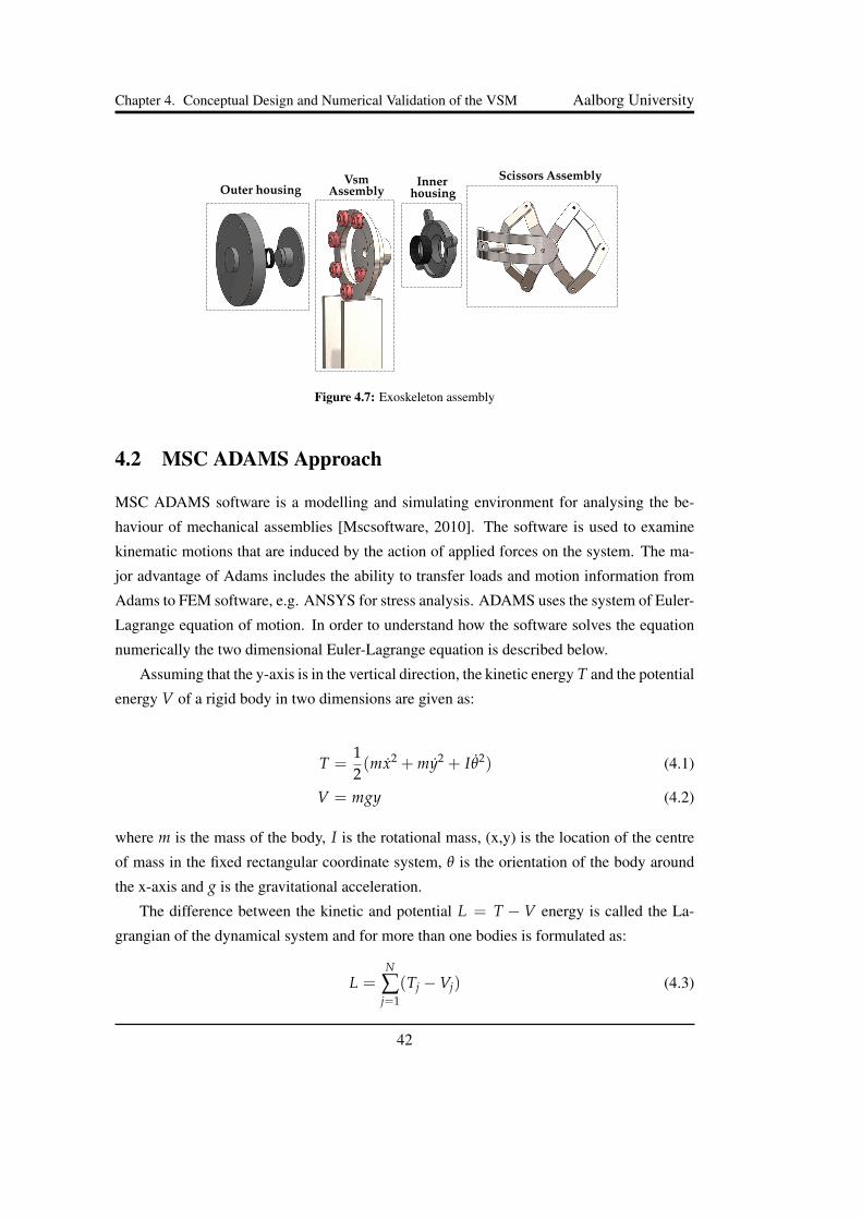
4.1.4 Exoskeleton Assembly
In Figure 4.7 the assembly of the parts described above can be seen. However, this is not
the whole exoskeleton design as this also includes the spring, the backplate and the cuffs to
connect it with the arm of the user.
41
Chapter 4. Conceptual Design and Numerical Validation of the VSM Aalborg University
Scissors AssemblyVsmOuter housing housing
InnerAssembly
Figure 4.7: Exoskeleton assembly
4.2 MSC ADAMS Approach
MSC ADAMS software is a modelling and simulating environment for analysing the be-
haviour of mechanical assemblies [Mscsoftware, 2010]. The software is used to examine
kinematic motions that are induced by the action of applied forces on the system. The ma-
jor advantage of Adams includes the ability to transfer loads and motion information from
Adams to FEM software, e.g. ANSYS for stress analysis. ADAMS uses the system of Euler-
Lagrange equation of motion. In order to understand how the software solves the equation
numerically the two dimensional Euler-Lagrange equation is described below.
Assuming that the y-axis is in the vertical direction, the kinetic energy T and the potential
energy V of a rigid body in two dimensions are given as:
T =12(mx2 + my2 + Iθ2) (4.1)
V = mgy (4.2)
where m is the mass of the body, I is the rotational mass, (x,y) is the location of the centre
of mass in the fixed rectangular coordinate system, θ is the orientation of the body around
the x-axis and g is the gravitational acceleration.
The difference between the kinetic and potential L = T − V energy is called the La-
grangian of the dynamical system and for more than one bodies is formulated as:
L =N
∑j=1
(Tj −Vj) (4.3)
42

Chapter 4. Conceptual Design and Numerical Validation of the VSM Aalborg University
where N is the number of bodies in the system.
The Euler-Lagrange equation for a multi-body system, which describes its motion is
formulated as:
ddt
(∂L∂q
)− ∂L
∂q+ ΦqTλ = Qex (4.4)
where q is the column matrix of generalized coordinates, λ represents the Langrange mul-
tipliers and Qex is the vector of generalized external forces acting along the coordinates q.
Φq is the Jacobian matrix of the constraint equations, which can be written as:
Φq =∂Φ∂q
(4.5)
An example of a simple pendulum and how ADAMS software is using the Lagrange
equation can be seen in Appendix E.
4.3 Design of the VSM
For the design of the VSM the dimensions, that used are those that found in Chapter 3 and
more specific in Table 3.7. The diameter for the cable is chosen 2mm. The VSM that is used
in MSC ADAMS can be seen in Figure 4.8. The start of the cable is attached to a fixed part
and the end is attached to a spring. The number of pulleys is six, those are fixed to the outer
(dark grey) and inner (light grey) parts. The outer part is allowed to rotate around the z-axis
and the inner part is fixed to the ground.
43

Chapter 4. Conceptual Design and Numerical Validation of the VSM Aalborg University
Figure 4.8: The VSM model in MSC ADAMS
In order to initiate a motion of the mechanism a preload has to be applied to the spring.
The value of the preload, which corresponds to the maximum spring elongation, has to be
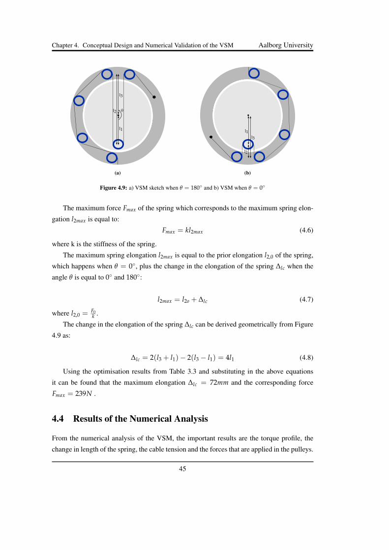
calculated. In Figure 4.9 the VSM can be seen, although only the two disks are displayed
for simplicity - the inner disk (light grey) and the outer disk (dark grey). The blue circles
represent the pulleys, where also the cable that connects them can be observed. l1 is the
distance from the center of the inner disk to the center of the pulley in the inner disk. The
distance from the center of the two upper pulleys to the center of the pulley in the inner disk
is the length l2. The distance between the center of the two upper pulleys and the center of
the inner disk is the length l3. The angle between the lengths l1 and l3 is represented by the
angle θ. In Figure 4.9a, the angle θ is equal to 180°, which happens when the arm is in the
initial position stretched down and in Figure 4.9b the angle θ is equal to 0◦, which occurs
when the arm is elevated 180◦ from hanging down.
44
Chapter 4. Conceptual Design and Numerical Validation of the VSM Aalborg University
l3
l2
l1
θ
(a)
l3
l2
l1
(b)
Figure 4.9: a) VSM sketch when θ = 180◦ and b) VSM when θ = 0◦
The maximum force Fmax of the spring which corresponds to the maximum spring elon-
gation l2max is equal to:
Fmax = kl2max (4.6)
where k is the stiffness of the spring.
The maximum spring elongation l2max is equal to the prior elongation l2,0 of the spring,
which happens when θ = 0◦, plus the change in the elongation of the spring ∆lc when the
angle θ is equal to 0◦ and 180◦:
l2max = l2o + ∆lc (4.7)
where l2,0 = F0k .
The change in the elongation of the spring ∆lc can be derived geometrically from Figure
4.9 as:
∆lc = 2(l3 + l1)− 2(l3 − l1) = 4l1 (4.8)
Using the optimisation results from Table 3.3 and substituting in the above equations
it can be found that the maximum elongation ∆lc = 72mm and the corresponding force
Fmax = 239N .
4.4 Results of the Numerical Analysis
From the numerical analysis of the VSM, the important results are the torque profile, the
change in length of the spring, the cable tension and the forces that are applied in the pulleys.
45

Chapter 4. Conceptual Design and Numerical Validation of the VSM Aalborg University
The results of the analytical and numerical analysis of the VSM can be seen in Figure 4.10.
Figure 4.10: Comparison of analytical and numerical results of the VSM model for the provided torque
From the figure above it can be seen that both the analytical and the numerical analyses
give similar results. The peaks of the resulting curves are listed in Table 4.1. The difference
between the peak loads is 102Nmm or 2% of the analytical result. The reason for this
deviation could be, the diameter of the pulley in ADAMS can only be set in certain standard
increments which result in differently dimensioned pulleys causing a discrepancy of the
resultant force in them. Also, ADAMS requires mass to calculate the Lagrange equation.
The mass used was close to zero, whereas in the analytical results the mass of the model
is not taken into account. Regarding the angle that the maximum torque is provided at, the
difference of the two analyses is at around 1.7◦. This corresponds to a deviation of 1.717%
compared to the peak angle of the analytical model.
Max Torque [Nmm] Angle [◦]
Analytical
solution4893.36 -99
Numerical
solution4791.15 -97.3
Table 4.1: Results of the two analysis for the maximum torque and angle
46
Chapter 4. Conceptual Design and Numerical Validation of the VSM Aalborg University
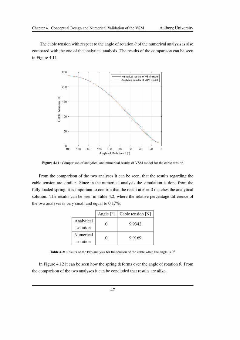
The cable tension with respect to the angle of rotation θ of the numerical analysis is also
compared with the one of the analytical analysis. The results of the comparison can be seen
in Figure 4.11.
Figure 4.11: Comparison of analytical and numerical results of VSM model for the cable tension
From the comparison of the two analyses it can be seen, that the results regarding the
cable tension are similar. Since in the numerical analysis the simulation is done from the
fully loaded spring, it is important to confirm that the result at θ = 0 matches the analytical
solution. The results can be seen in Table 4.2, where the relative percentage difference of
the two analyses is very small and equal to 0.17%.
Angle [◦] Cable tension [N]
Analytical
solution0 9.9342
Numerical
solution0 9.9169
Table 4.2: Results of the two analysis for the tension of the cable when the angle is 0◦
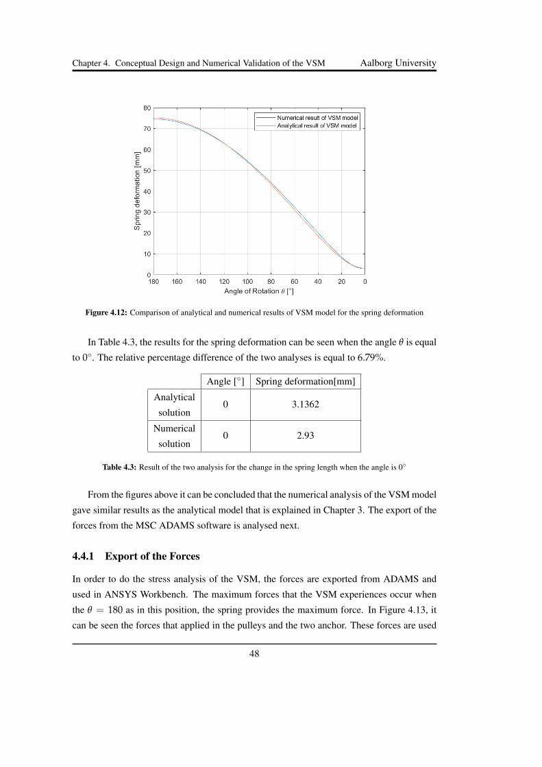
In Figure 4.12 it can be seen how the spring deforms over the angle of rotation θ. From
the comparison of the two analyses it can be concluded that results are alike.
47
Chapter 4. Conceptual Design and Numerical Validation of the VSM Aalborg University
Figure 4.12: Comparison of analytical and numerical results of VSM model for the spring deformation
In Table 4.3, the results for the spring deformation can be seen when the angle θ is equal
to 0◦. The relative percentage difference of the two analyses is equal to 6.79%.
Angle [◦] Spring deformation[mm]
Analytical
solution0 3.1362
Numerical
solution0 2.93
Table 4.3: Result of the two analysis for the change in the spring length when the angle is 0◦
From the figures above it can be concluded that the numerical analysis of the VSM model
gave similar results as the analytical model that is explained in Chapter 3. The export of the
forces from the MSC ADAMS software is analysed next.
4.4.1 Export of the Forces
In order to do the stress analysis of the VSM, the forces are exported from ADAMS and
used in ANSYS Workbench. The maximum forces that the VSM experiences occur when
the θ = 180 as in this position, the spring provides the maximum force. In Figure 4.13, it
can be seen the forces that applied in the pulleys and the two anchor. These forces are used
48

Chapter 4. Conceptual Design and Numerical Validation of the VSM Aalborg University
in Section 5.2 for the analysis of the structure.
y
x
F1F2F4
F5
F6 F3
F7
F8
Figure 4.13: Forces exported from MSC ADAMS
It is difficult to find the spring with the same property as obtained in the optimisation
result in Chapter 3. Therefore, a spring was selected with similar properties, which can be
seen in Table 4.4.
MaterialInitial length Lo
[mm]
Max length
[mm]
Max Force
[N]
Preload
[N]
Stiffness
[N/mm]
Piano wire 127 204.98 301.89 27.18 3.52
Table 4.4: Spring properties that used in the VSM
The torque provided from the VSM is found and compared with the analytical results.
Both results use the properties of the available spring. Furthermore when θ = 180◦, the
elongation of the spring is 72mm and so the maximum force of the spring in this position
is Fmax = 280.62N. This means that the maximum force of the spring is greater than
the one that was found in the optimisation, where the stiffness of the spring was equal to
3.1675N/mm and, including the pretension F0, the maximum force of the spring was found
to be 239N for θ = 180◦. However, as mentioned before, it is not easy to find the exact
stiffness and the pretension that the optimisation part gave. The comparison of the two
analyses can be seen in Figure 4.14.
49
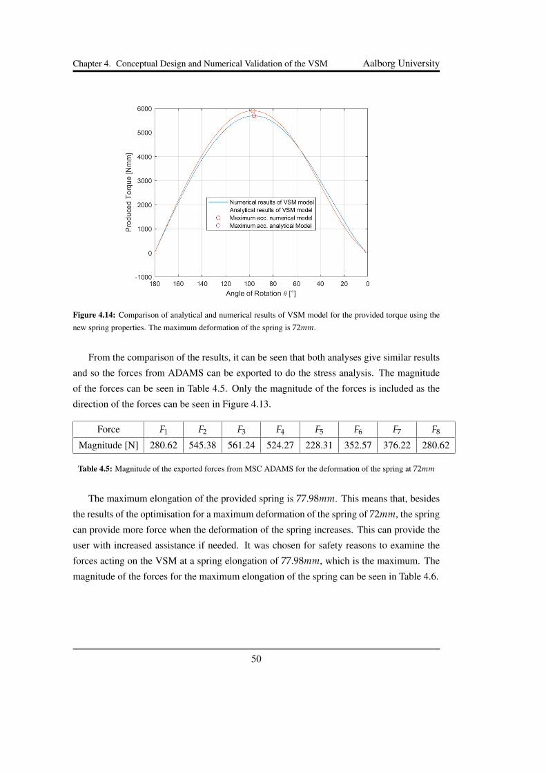
Chapter 4. Conceptual Design and Numerical Validation of the VSM Aalborg University
Figure 4.14: Comparison of analytical and numerical results of VSM model for the provided torque using the
new spring properties. The maximum deformation of the spring is 72mm.
From the comparison of the results, it can be seen that both analyses give similar results
and so the forces from ADAMS can be exported to do the stress analysis. The magnitude
of the forces can be seen in Table 4.5. Only the magnitude of the forces is included as the
direction of the forces can be seen in Figure 4.13.
Force F1 F2 F3 F4 F5 F6 F7 F8
Magnitude [N] 280.62 545.38 561.24 524.27 228.31 352.57 376.22 280.62
Table 4.5: Magnitude of the exported forces from MSC ADAMS for the deformation of the spring at 72mm
The maximum elongation of the provided spring is 77.98mm. This means that, besides
the results of the optimisation for a maximum deformation of the spring of 72mm, the spring
can provide more force when the deformation of the spring increases. This can provide the
user with increased assistance if needed. It was chosen for safety reasons to examine the
forces acting on the VSM at a spring elongation of 77.98mm, which is the maximum. The
magnitude of the forces for the maximum elongation of the spring can be seen in Table 4.6.
50

Chapter 4. Conceptual Design and Numerical Validation of the VSM Aalborg University
Force F1 F2 F3 F4 F5 F6 F7 F8
Magnitude [N] 301.87 584.12 603.34 562.33 245.77 370.73 387.82 301.67
Table 4.6: Magnitude of the exported forces from MSC ADAMS for the maximum spring elongation of
77.98mm
Spring deformation
[mm]
Maximum Torque
[Nmm]
Pretension Fo
[N]
72 5907.94 27.18
74 6114.92 34.22
76 6323.83 41.26
Table 4.7: Maximum torque that the spring can provide in the three different levels 72mm, 74mm, 76mm and
the pretension of the spring.
51

Chapter 5
Design and Construction of the Exoskele-ton
In this chapter, the design loads calculated from the numerical analysis from MSC ADAMS
are used to perform a structural analysis of the structure. Using the results the design is fur-
ther optimised to reduce the weight of the structure. For this purpose topology optimisation
in ANSYS is used.
5.1 Material Selection
To select materials that can be used in the exoskeleton, the stresses are crucial. If possible,
light materials should be used to reduce the weight of the structure. However, those tend to
increase the cost of the structure. Some options of the material that can realistically be used
are presented below.
It is possible to build the components of the exoskeleton from composites. However, this
class of materials is not elaborated on, because it seems unfitting in such an early stage of
development because the production of composite parts is very cost-intensive.
Polymers
Polymers can reduce the cost and also the weight of the structure in a significant way. Some
of the polymers that can be used are Acrylonitrile Butadiene Styrene (ABS) and Polylactic
acid (PLA). Both materials have similar cost and strength, but the PLA is more preferable for
prototyping because of its ease of printing, aesthetically appealing parts, and high accuracy
52

Chapter 5. Design and Construction of the Exoskeleton Aalborg University
[Feeney, 2019]. Both materials can be used for 3D printing. The mechanical properties
for the two materials can be seen in Figure 5.1. However, the mechanical properties vary
drastically depending on how it is manufactured [Farah et al., 2016]. It was decided to make
the pulleys, the inner and the outer housings from PLA as in this way the final weight and
costs are reduced.
MaterialDensity
[kg/m^3]Young’s modulus
[GPa]Tensile strength
[MPa]ABS 1000-1400 2-2.6 37-110
PLA 1300 3.5 50
Table 5.1: Mechanical properties of PLA and ABS [Ltd, 2021]
Metals
When high strength and stiffness are required metals alloys are necessary. Steel is the com-
monly used metal because of its good mechanical properties and the large variety of strength.
However, if choosing a steel with higher strength also the cost are increased. Aluminium is
a good choice because of its low density. It can replace steel and provides a lighter structure
without compromising strength. Compared to steel, aluminium can deform and bend more
easily. Other commonly used lightweight alloys are titanium or magnesium alloys. Due to
their high cost, those are disregarded here. It is decided to use high strength Aluminium
7075-T6 for the Slot Link. For ease of machining and welding, it is decided to use Alu-
minium 5083-O for the outer frame and the inner disk. To keep the friction low and allow
the Connection Slot to slide inside the Slot Link, it is decided to make the Connection Slot
from brass. The material used for the SSM provided by AAU is EN-1.4404.
5.2 Finite Element Analysis
In this section the structural analysis of the Scissors Assembly and VSM Assembly will
be carried out. The software used for these analysis is Ansys Workbench. The analyses
conducted are linear static structural simulations.
53

Chapter 5. Design and Construction of the Exoskeleton Aalborg University
Material Properties
Ansys requires material parameters to conduct the analysis. The property of EN-1.4404,
Aluminium 7075-T6 and Aluminium 5083-O, that are used for the analyses, are mentioned
in Table 5.2.
MaterialDensity
[kg/m^3]Young’s Modulus
[GPa]Poisson’s
RatioYeild Strength
[MPa]EN-1.4404 8000 200 0.3 220
Aluminium 7075-T6 2810 71.7 0.33 503
Aluminium 5083-O 2660 71 0.33 145
Table 5.2: Material property data is taken from [MATWEB, 2021]
Safety Factor
It is always important to consider a proper Factor of safety (FOS). As a general recom-
mendation for commercial aircrafts, which is a structure where weight and safety are both
of crucial importance, a FOS of 1.2− 1.5 is recommended [Norton, 2010]. Since there is
no specific FOS for exoskeletons, a safety factor of 1.3 is chosen. This value is valid be-
cause it is within the range of an aircraft, but the risk for the users of the exoskeleton is
less than in the aviation industry. The von Mises failure criterion is used for the analysis.
For Aluminium 7075-T6 the maximum allowable stress including the FOS is 386MPa, for
Aluminium 5083-O the stress is 111MPa and for EN-1.4404 the maximum allowable stress
is 169MPa.
5.2.1 Structural Analysis of Scissors Mechanism
The Scissors mechanism is designed to transfer the torque from the VSM to the backplate.
The model is simulated in a way that approximately represents real-life loading and bound-
ary conditions.
Loading and Boundary condition
The maximum torque calculated for the maximum spring deformation at 77.98mm using the
analytical solution is found to be 6532Nmm. Three different loading condition are consid-
ered where the position of Connection Slot is changed to 8°, 59° and 82°, these configura-
54
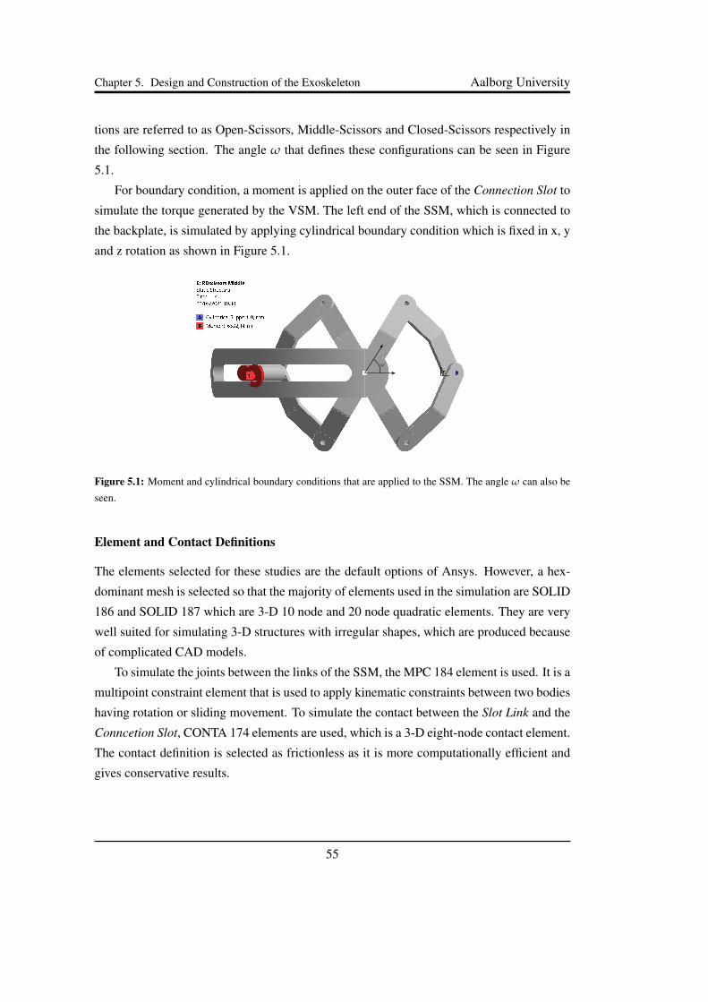
Chapter 5. Design and Construction of the Exoskeleton Aalborg University
tions are referred to as Open-Scissors, Middle-Scissors and Closed-Scissors respectively in
the following section. The angle ω that defines these configurations can be seen in Figure
5.1.
For boundary condition, a moment is applied on the outer face of the Connection Slot to
simulate the torque generated by the VSM. The left end of the SSM, which is connected to
the backplate, is simulated by applying cylindrical boundary condition which is fixed in x, y
and z rotation as shown in Figure 5.1.
ω
Figure 5.1: Moment and cylindrical boundary conditions that are applied to the SSM. The angle ω can also be
seen.
Element and Contact Definitions
The elements selected for these studies are the default options of Ansys. However, a hex-
dominant mesh is selected so that the majority of elements used in the simulation are SOLID
186 and SOLID 187 which are 3-D 10 node and 20 node quadratic elements. They are very
well suited for simulating 3-D structures with irregular shapes, which are produced because
of complicated CAD models.
To simulate the joints between the links of the SSM, the MPC 184 element is used. It is a
multipoint constraint element that is used to apply kinematic constraints between two bodies
having rotation or sliding movement. To simulate the contact between the Slot Link and the
Conncetion Slot, CONTA 174 elements are used, which is a 3-D eight-node contact element.
The contact definition is selected as frictionless as it is more computationally efficient and
gives conservative results.
55

Chapter 5. Design and Construction of the Exoskeleton Aalborg University
Stress Result for Scissors Mechanism
Due to contacts and fixed boundary condition used in the simulation, there are stress con-
centrations developed in these areas. According to the Saint-Venant’s principle, the effect of
local disturbances to the uniform stress field remains local. The results away from these dis-
turbances are not affected. To get the correct stress values, new sections are created for each
link of the SSM, which are 4mm away from the point of stress concentration as shown in
Figure 5.2. For the Slot Link, the stresses are probed away from stress concentration caused
by the contact faces of the Connection Slot to the Slot Link. The convergence plots for all
the results below are shown in Appendix F.
Link 1
Link 2
Link 4
Link 3Link 5
Link 6
Figure 5.2: SSM showing different section in the links that are selected to probe for maximum stress
Open-Scissors Configuration
The stress distribution for the Open-Scissors configuration can be seen in Figure 5.3. In
Table 5.3, the maximum equivalent stresses for the 6 links and the Slot Link are observed.
Figure 5.3: Stress distribution for the Open-Scissors configuration
56

Chapter 5. Design and Construction of the Exoskeleton Aalborg University
Scissor Link Maximum Stress (MPa)1 121.66
2 116.49
3 560.22
4 517.75
5 464.1
6 516.26
Slot Link 226.12
Table 5.3: Maximum stress for the 6 links and the Slot Link for the Open-Scissors configuration
Middle-Scissors Configuration
The results of the stress analysis for the Middle-Scissors configuration can be seen in Figure
5.4 and also the maximum equivalent stresses for the 6 links and the Slot Link in Table 5.4.
Figure 5.4: Stress distribution for the Middle-Scissors configuration
Scissor Link Maximum Stress (MPa)1 43
2 43
3 480.94
4 498.12
5 498.01
6 490.29
Slot Link 272.86
Table 5.4: Maximum equivalent stresses for the 6 links and the Slot Link for the Middle-Scissors configuration
57
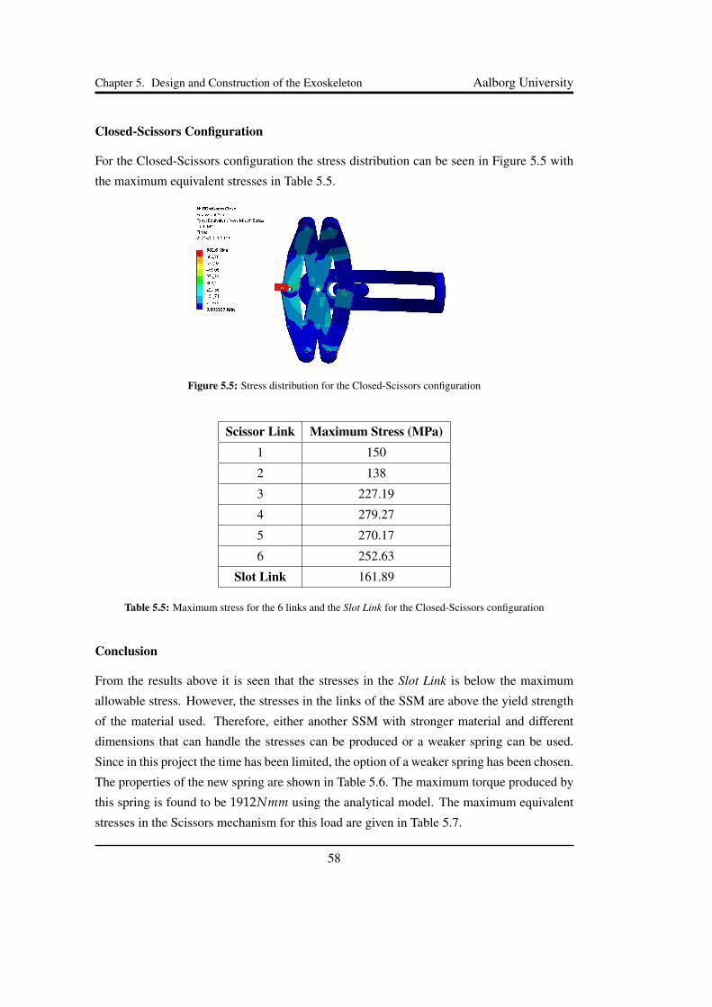
Chapter 5. Design and Construction of the Exoskeleton Aalborg University
Closed-Scissors Configuration
For the Closed-Scissors configuration the stress distribution can be seen in Figure 5.5 with
the maximum equivalent stresses in Table 5.5.
Figure 5.5: Stress distribution for the Closed-Scissors configuration
Scissor Link Maximum Stress (MPa)1 150
2 138
3 227.19
4 279.27
5 270.17
6 252.63
Slot Link 161.89
Table 5.5: Maximum stress for the 6 links and the Slot Link for the Closed-Scissors configuration
Conclusion
From the results above it is seen that the stresses in the Slot Link is below the maximum
allowable stress. However, the stresses in the links of the SSM are above the yield strength
of the material used. Therefore, either another SSM with stronger material and different
dimensions that can handle the stresses can be produced or a weaker spring can be used.
Since in this project the time has been limited, the option of a weaker spring has been chosen.
The properties of the new spring are shown in Table 5.6. The maximum torque produced by
this spring is found to be 1912Nmm using the analytical model. The maximum equivalent
stresses in the Scissors mechanism for this load are given in Table 5.7.
58

Chapter 5. Design and Construction of the Exoskeleton Aalborg University
MaterialInitial length Lo
[mm]
Max length
[mm]
Max Force
[N]
Preload
[N]
Stiffness
[N/mm]
Piano wire 114 204.72 83.63 12.70 0.84
Table 5.6: Spring properties of the weaker spring
Scissors-Open Scissors-Middle Scissors-CloseLink Maximum Stress (MPa) Maximum Stress (MPa) Maximum Stress (MPa)
1 35 12 43
2 33 13 41
3 163.95 140.82 67
4 151.58 145.79 82
5 135.77 145.92 79.29
6 151.18 143.34 73.57
Table 5.7: Maximum stresses in each link of the Scissors using a weaker spring
From the results for the six links for the three configurations of the SSM, as expected
the stresses are reduced. Since the material that the provided SSM is made off is EN-1.4404
and the maximum allowable stress is 169MPa it can be concluded, that the SSM with the
weaker spring can withstand the stress.
5.2.2 Structural Analysis of VSM Assembly
In this section the structural analysis of the VSM Assembly is described. The structural
analysis includes the the Outer Frame and the Inner Disc. It has to be noted that for the
structural analysis of the VSM Assembly the load results for assistance with half the shoulder
torque is used and not the one for the weaker spring. The reason for not using the weaker
spring, as for the analysis of the SSM, is, that if the VSM can hold the stresses for the
original spring then only the SSM has to be changed.
Analysis of Outer Frame
The model is simplified by removing the pins and the pulleys. All the loads used in the
simulation are taken from MSC ADAMS in Chapter 4. A fixed boundary condition is applied
at the side where the Inner Housing Assembly is in contact with the Outer Frame. A bearing
59
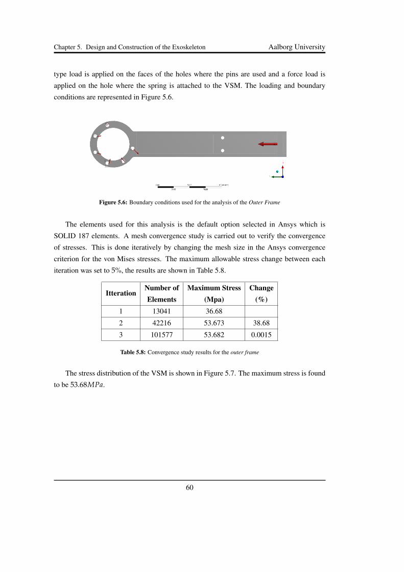
Chapter 5. Design and Construction of the Exoskeleton Aalborg University
type load is applied on the faces of the holes where the pins are used and a force load is
applied on the hole where the spring is attached to the VSM. The loading and boundary
conditions are represented in Figure 5.6.
Figure 5.6: Boundary conditions used for the analysis of the Outer Frame
The elements used for this analysis is the default option selected in Ansys which is
SOLID 187 elements. A mesh convergence study is carried out to verify the convergence
of stresses. This is done iteratively by changing the mesh size in the Ansys convergence
criterion for the von Mises stresses. The maximum allowable stress change between each
iteration was set to 5%, the results are shown in Table 5.8.
ItterationNumber ofElements
Maximum Stress(Mpa)
Change(%)
1 13041 36.68
2 42216 53.673 38.68
3 101577 53.682 0.0015
Table 5.8: Convergence study results for the outer frame
The stress distribution of the VSM is shown in Figure 5.7. The maximum stress is found
to be 53.68MPa.
60
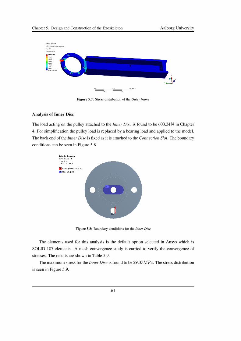
Chapter 5. Design and Construction of the Exoskeleton Aalborg University
Figure 5.7: Stress distribution of the Outer frame
Analysis of Inner Disc
The load acting on the pulley attached to the Inner Disc is found to be 603.34N in Chapter
4. For simplification the pulley load is replaced by a bearing load and applied to the model.
The back end of the Inner Disc is fixed as it is attached to the Connection Slot. The boundary
conditions can be seen in Figure 5.8.
Figure 5.8: Boundary conditions for the Inner Disc
The elements used for this analysis is the default option selected in Ansys which is
SOLID 187 elements. A mesh convergence study is carried to verify the convergence of
stresses. The results are shown in Table 5.9.
The maximum stress for the Inner Disc is found to be 29.37MPa. The stress distribution
is seen in Figure 5.9.
61

Chapter 5. Design and Construction of the Exoskeleton Aalborg University
ItterationNumber ofElements
Maximum Stress(MPa)
Change(%)
1 3823 25.923
2 9665 27.52 5.97
3 45161 29.37 3.05
Table 5.9: Convergence study results for the Inner Disc
Figure 5.9: The stress distribution of the Inner Disc
Conclusion
The structural analysis of the VSM Assembly shows that the stresses are very low in both, the
Outer Frame and the Inner Disc as compared to the yield strength of the material. Therefore,
to reduce the weight of the component it is decided to carry out topology optimisation on
the Outer Frame as this part contributes significantly to the weight of the whole assembly.
5.3 Topology Optimisation
The following section is based on [ANSYS, 2021] unless marked differently. Topology opti-
misation computes an optimal design of a structure, where design objectives and constraints
are specified. It can also be implemented to specific regions that the user desires to change.
In this project, the topology optimisation tool in Ansys is used. To conduct the topology
optimisation there are three ways:
• Level Set Based Topology
• Lattice Optimisation
62

Chapter 5. Design and Construction of the Exoskeleton Aalborg University
• Density Based
The first method is based on the boundaries of the shapes. The design variable for this
method are the boundaries of the structure and they are adjusted to optimise the structure.
The lattice optimization method computes an optimal variable density lattice distribution in
the geometry. It is a useful method for optimisation of 3D printed parts. The third method is
based on the density of each element. In this project the density based method is used and
so only this is elaborated on.
5.3.1 Density Based Method
In order to increase the stiffness of the structure, the strain energy has to be reduced. This
is done by assigning a pseudo-density to each element. An approach for the topology op-
timization problem is the Solid Isotropic Material with Penalization (SIMP) approach. In
this approach the design variables ρi, where i are the elements, are the element densities
that are assigned. The value of the density can be varied from 0, which means that the el-
ement is removed, to 1, where the element is preserved. Generally, the original problem
consists of 0 or 1 density elements. However, this problem can not be solved because of
the large search-space containing N!/((N −M)!M!) possibilities, where N is the number
of material elements and M the number of all the elements [Nobel-Jørgensen, 2016]. It can
be easily concluded that when the number of material elements is increased, the time to
solve the problem rises exponentially. The SIMP approach allows using intermediate values
between 0 and 1, which reduces the search space.
General Topology Optimisation Problem
In general, the topology optimisation problem is seeking to minimise or maximise the ob-
jective function. The objective function can be the compliance, the natural frequencies etc.
The mathematical optimisation problem can be written as [Kohnke, 1999]:
Maximize or Minimize : f
Subjected to : 0 < ρi ≤ 1 (i = 1, 2, ..., M)
gjl ≤ gj ≤ gjr (i = 1, 2, ..., N)
where M is the number of elements, gj is the computed jth constraint value, gjl and gjr
are the lower and upper bounds of the jth constraint and N is the number of the constraints.
63

Chapter 5. Design and Construction of the Exoskeleton Aalborg University
Topology Optimisation for Compliance Minimisation
For this project, the aim of the topology optimisation that is carried out is to minimise the
compliance of the structure i.e. to maximize the stiffness. The general mathematical opti-
mization can be rewritten now as [Lund et al., 2019]:
Minimize : C(U)
Subjected to : 0 < ρi ≤ 1 (i = 1, 2, ..., M)
K = UF
V∗ = aV
Ei = ρpi E∗
where C(U) is the compliance of the structure, K is the global stiffness matrix, U is the
global displacement vector, F is the global force matrix, V∗ is the material volume, V is
the design domain volume, a is the volume fraction of available material, Ei is the Young
modulus of each element, p is a penalty factor and E∗ is the Young modulus for ρ = 1.
The volume fraction a is the amount of the desired reduction of the volume of the struc-
ture. The penalty factor is used to reduce the greyscale elements [Nobel-Jørgensen, 2016],
where greyscale elements are the elements that have a density between 0 and 1. Using the
penalty factor these elements become closer to dark or white colours and in this way the
final design is more clear and easier to be manufactured. Typically the value for this penalty
factor is 3 [Sigmund, 2001].
The compliant problem can be solved either by using Optimality Criteria (OC) methods
or gradient-based algorithms such as Sequential Linear Programming (SLP) and Method of
Moving Asymptotes (MMA). The Optimality Criteria is an iterative solver, where the de-
sign variables on each point are updated based on the optimality conditions. In the points
where the strain energy is high, material is added. The default solver in ANSYS is the Se-
quential Convex Programming (SCP), which is an extension of MMA. MMA is a nonlinear
programming algorithm where the solution is approximated by solving a sequence of convex
and separable sub-problems. It is an inexpensive method since the sub-problems are more
easily solved [ANSYS, 2021].
64
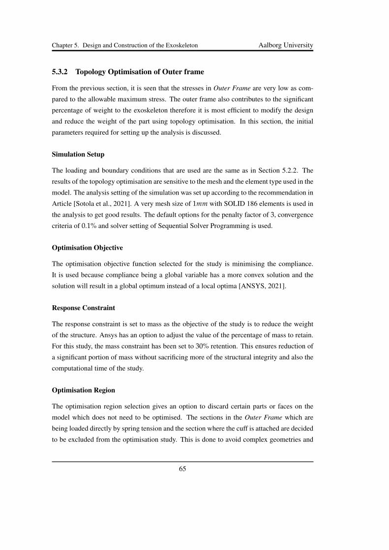
Chapter 5. Design and Construction of the Exoskeleton Aalborg University
5.3.2 Topology Optimisation of Outer frame
From the previous section, it is seen that the stresses in Outer Frame are very low as com-
pared to the allowable maximum stress. The outer frame also contributes to the significant
percentage of weight to the exoskeleton therefore it is most efficient to modify the design
and reduce the weight of the part using topology optimisation. In this section, the initial
parameters required for setting up the analysis is discussed.
Simulation Setup
The loading and boundary conditions that are used are the same as in Section 5.2.2. The
results of the topology optimisation are sensitive to the mesh and the element type used in the
model. The analysis setting of the simulation was set up according to the recommendation in
Article [Sotola et al., 2021]. A very mesh size of 1mm with SOLID 186 elements is used in
the analysis to get good results. The default options for the penalty factor of 3, convergence
criteria of 0.1% and solver setting of Sequential Solver Programming is used.
Optimisation Objective
The optimisation objective function selected for the study is minimising the compliance.
It is used because compliance being a global variable has a more convex solution and the
solution will result in a global optimum instead of a local optima [ANSYS, 2021].
Response Constraint
The response constraint is set to mass as the objective of the study is to reduce the weight
of the structure. Ansys has an option to adjust the value of the percentage of mass to retain.
For this study, the mass constraint has been set to 30% retention. This ensures reduction of
a significant portion of mass without sacrificing more of the structural integrity and also the
computational time of the study.
Optimisation Region
The optimisation region selection gives an option to discard certain parts or faces on the
model which does not need to be optimised. The sections in the Outer Frame which are
being loaded directly by spring tension and the section where the cuff is attached are decided
to be excluded from the optimisation study. This is done to avoid complex geometries and
65
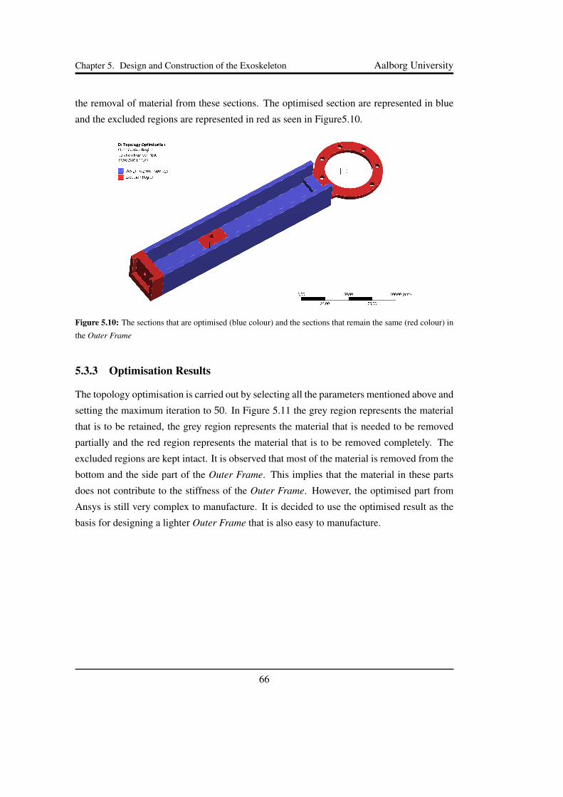
Chapter 5. Design and Construction of the Exoskeleton Aalborg University
the removal of material from these sections. The optimised section are represented in blue
and the excluded regions are represented in red as seen in Figure5.10.
Figure 5.10: The sections that are optimised (blue colour) and the sections that remain the same (red colour) in
the Outer Frame
5.3.3 Optimisation Results
The topology optimisation is carried out by selecting all the parameters mentioned above and
setting the maximum iteration to 50. In Figure 5.11 the grey region represents the material
that is to be retained, the grey region represents the material that is needed to be removed
partially and the red region represents the material that is to be removed completely. The
excluded regions are kept intact. It is observed that most of the material is removed from the
bottom and the side part of the Outer Frame. This implies that the material in these parts
does not contribute to the stiffness of the Outer Frame. However, the optimised part from
Ansys is still very complex to manufacture. It is decided to use the optimised result as the
basis for designing a lighter Outer Frame that is also easy to manufacture.
66
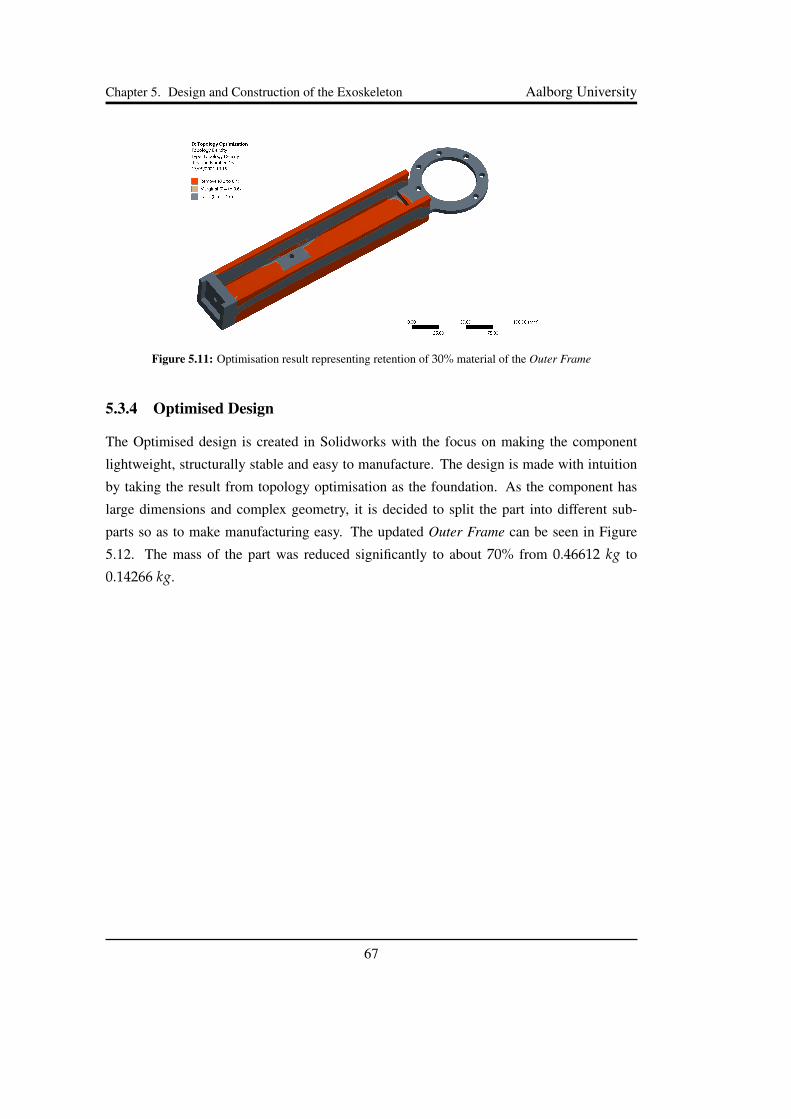
Chapter 5. Design and Construction of the Exoskeleton Aalborg University
Figure 5.11: Optimisation result representing retention of 30% material of the Outer Frame
5.3.4 Optimised Design
The Optimised design is created in Solidworks with the focus on making the component
lightweight, structurally stable and easy to manufacture. The design is made with intuition
by taking the result from topology optimisation as the foundation. As the component has
large dimensions and complex geometry, it is decided to split the part into different sub-
parts so as to make manufacturing easy. The updated Outer Frame can be seen in Figure
5.12. The mass of the part was reduced significantly to about 70% from 0.46612 kg to
0.14266 kg.
67

Chapter 5. Design and Construction of the Exoskeleton Aalborg University
Figure 5.12: Optimised design of Outer Frame
Stress result for optimised design
The boundary conditions applied are the same as discussed in subsection 5.2.2. The stress
distribution for the optimised design can be seen in Figure 5.13. It is observed that the
overall stress has increased slightly than the initial design, however, the maximum stress is
still below the allowable limit of 111 MPa. The convergence of the von Mises stresses is
done iteratively by changing the mesh size in Ansys and the results are shown in Table 5.10.
IterationNumber ofElements
Maximum Stress(MPa)
Change(%)
1 5492 62.58
2 19855 83.8 29
3 32250 83.86 0.007
Table 5.10: Convergence study of maximum von Mises stresses in the optimised Outer Frame
68

Chapter 5. Design and Construction of the Exoskeleton Aalborg University
Figure 5.13: Von Mises stress distribution of the optimised Outer Frame
All the engineering drawings for the designed parts can be found in Appendix G.
69

Chapter 6
Additional Design Ideas
The following chapter presents a collection of ideas and possibilities to implement in order
to include a second DOF in the assistance of the exoskeleton. This DOF represent the
abduction-adduction movement. The first idea describes the possibility of having two VSM
in the exoskeleton connected with one cable. The other idea is to have only one VSM but it
can be shifted and adjusted to the necessary movement. In the end, a backplate mechanism
is presented to ensure that the mechanism is put in the right position and can provide the
maximum torque.
6.1 Addition of a Second Degree of Freedom
The preliminary design as presented gives assistance for motion in the sagittal plane only.
In this section, the addition of one more assisted plane is explored.
Simply adding a second torque providing device is not a sufficient solution, because the
sagittal and the coronal plane are not independent of each other. In other words, if the arm is
lifted in one plane, kept in an elevated position and moved to the other plane, the first torque
providing device has to go back to its fully loaded condition while the second device has to
become active. Additionally, the SSM does not behave like a rigid link, but compresses after
a certain range of pure rotation around the fixed point at the backplate. The behaviour of the
SSM also depends on the positioning of the joint at the backplate and the joint connected
to the VSM, for motion in the sagittal plane. In the following, two different approaches are
presented, which work around this problem in different ways.
70
Chapter 6. Additional Design Ideas Aalborg University
6.1.1 Two VSM One Cable
In order to work around the problems with two independent torque providing mechanisms,
one solution might be to connect the two compliant elements. The VSM as described in
Chapter 2 is a desirable mechanism, as its torque varies and can be adjusted not only to
the motion in the sagittal plane but also in the coronal plane. Thus in the following, an
exoskeleton with two VSMs, one for the sagittal and one for the coronal plane, is suggested.
Another advantage of using the same mechanism twice with different parameters is that it
can be easily connected. In the present case, such a connection would be to guide the cable
from one VSM to the second one. In this manner the cable forces of both VSMs are equal
and the number of compliant elements can be reduced to one.
The advantage of such a configuration is, that from a position where the arm is hanging
down with all angles θ1...7 = 0◦ from Figure 3.1, both, motion in sagittal and coronal plane
are supported from the beginning. However, difficulties arise when a mixed motion of some
angle between the two planes is supposed to be supported. Because the cable tension is
equal for both VSMs, the torque is influenced by the dimensions, that is l1 and l3. Since
the combined torque of both VSMs needs to be composed differently for varying angles
between the two planes, the dimensions l1 and l3 need to adjust themselves automatically to
perfectly balance the weight of the arm. This is very difficult to implement purely passively,
but is possible to implement in a pseudo-passive exoskeleton. Figure 6.1a shows the xm-,
ym- and zm-component of the torque vector produced by the weight of the arm if the arm is
being rotated from the sagittal to the coronal plane at an elevation angle of 90◦. Figure 6.1b
shows the absolute torque as described in Section 3.4 for a VSM that is rotated with the arm
as a function of the shoulder angle γ and the length l1.
71

Chapter 6. Additional Design Ideas Aalborg University
(a) (b)
(c)
Figure 6.1: (a) Composition of the torque vector for a transition of the elevated arm from the sagittal to the
coronal plane, the torque vector is described in the main coordinate system introduced in Section 3.1.
(b) Absolute torque of a VSM for varying l1 and the shoulder angle γ; the fixed dimensions are the ones
obtained with the optimisation described in Section 3.3.
(c) Absolute torque of a VSM with the dimensions as obtained in Section 3.4 for selected shoulder angles γ as
a function of l1.
As expected the zm-component is 0Nmm for the entire range and the shape of the
nonzero components follows a sine and cosine curve, respectively. As it can be seen in
Figure 6.1a there is no linear relation between the x- or y-component of the required torque
and the variation of the torque produced by a change of l1. This is especially clear when a
look at Figure 6.1c is taken, which documents the change in absolute produced torque over
l1 = 0mm...18mm for selected shoulder angles γ.
72

Chapter 6. Additional Design Ideas Aalborg University
Adjustment of l1
To produce the required torque behaviour, the governing differential equation has to be
solved for l1 with a certain torque input. This is not a trivial task, because l1 influences
the torque only indirectly by defining the length l2. Therefore the governing differential
equation of the VSM torque is solved numerically for l1 by comparing the required torque
with the full range of possible torque values for a certain angle γ. The resulting curves for
l1 over ξ, which describes the angle between the sagittal plane and the plane of motion, is
presented in Figure 6.2.
Figure 6.2: Curves for the length l1 over ξ for selected elevation angles
Note that the above Figure 6.2 is only valid for the x-component of the torque. The
y-component shows the same behaviour but is flipped so it starts with zero length. Further
elaboration on the required length l1 as well as the consequences for the active component
can be found in Appendix H.
Connection between the two VSM
With the torque of each of the two individual VSM now being able to adjust to the require-
ment, the problem of connecting the two mechanisms physically remains. The most compact
solution is to use the SSM as described in Section 2.2. To be able to apply a force on the
arm, the second VSM, which counters the y-component of the torque of the weight of the
arm, has to transfer torque to the SSM. This can be done with the same mechanism as used
73
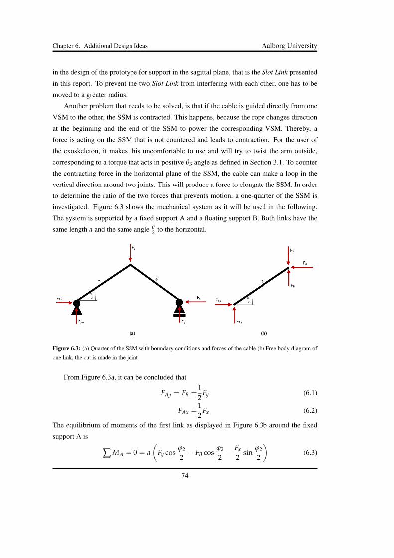
Chapter 6. Additional Design Ideas Aalborg University
in the design of the prototype for support in the sagittal plane, that is the Slot Link presented
in this report. To prevent the two Slot Link from interfering with each other, one has to be
moved to a greater radius.
Another problem that needs to be solved, is that if the cable is guided directly from one
VSM to the other, the SSM is contracted. This happens, because the rope changes direction
at the beginning and the end of the SSM to power the corresponding VSM. Thereby, a
force is acting on the SSM that is not countered and leads to contraction. For the user of
the exoskeleton, it makes this uncomfortable to use and will try to twist the arm outside,
corresponding to a torque that acts in positive θ3 angle as defined in Section 3.1. To counter
the contracting force in the horizontal plane of the SSM, the cable can make a loop in the
vertical direction around two joints. This will produce a force to elongate the SSM. In order
to determine the ratio of the two forces that prevents motion, a one-quarter of the SSM is
investigated. Figure 6.3 shows the mechanical system as it will be used in the following.
The system is supported by a fixed support A and a floating support B. Both links have the
same length a and the same angle θ2 to the horizontal.
(a) (b)
Figure 6.3: (a) Quarter of the SSM with boundary conditions and forces of the cable (b) Free body diagram of
one link, the cut is made in the joint
From Figure 6.3a, it can be concluded that
FAy = FB =12
Fy (6.1)
FAx =12
Fx (6.2)
The equilibrium of moments of the first link as displayed in Figure 6.3b around the fixed
support A is
∑ MA = 0 = a(
Fy cosϕ2
2− FB cos
ϕ2
2− Fx
2sin
ϕ2
2
)(6.3)
74

Chapter 6. Additional Design Ideas Aalborg University
and it follows with Equation (6.1), that
Fy
Fx= tan
ϕ2
2(6.4)
The range of ϕ2 is determined from Equation (2.11) and Table 2.1 and ranges from
ϕ2 = 5.4◦...167.6◦. Figure 6.4 displays the range, which the ratio of Fy to Fx has to have
over the range of ϕ2.
Figure 6.4: Ratio of Fy/Fx so that the SSM is stabilised
As it is seen, stabilisation of the SSM over the whole range is impossible to be achieved,
because equation (6.4) approaches infinity for ϕ2 −→ 180◦. However, a ratio of 1 ≤ FyFx≤ 2
is obtainable with a vertical loop around two joints as shown in Figure 6.5.
Figure 6.5: SSM with continuous cable from one VSM to the other with a vertical loop for stabilisation
The two pulleys that enforce the 180◦-change of direction in the vertical take two times
the cable force which correlates to Fy. To get a ratio of FyFx
= 1, the VSMs must be attached
horizontally, so that both points of zero torque are lying on the horizontal. Then the first and
75

Chapter 6. Additional Design Ideas Aalborg University
the last pulleys that are touched by the cable also experience two times the cable force. If
this position of the VSMs is combined with an angle ϕ2 = 90◦, the SSM is stabilised. If
the VSM rotates to its minimum potential energy position, the ratio of FyFx
approaches two,
which corresponds to ϕ2 ≈ 127◦. For ϕ2 outside the range of 90◦...127◦ no force ratio can
be obtained with this configuration, which stabilises the SSM.
Another unsolved problem is, that the length of the cable has to be accounted for over
the full range of motion of the SSM. If a pulley radius of 0mm is assumed, the cable length
from one end to the other of the SSM is given by:
lC−SSM = 4α(
cosϕ2
2+ sin
ϕ2
2
)(6.5)
Figure 6.6 shows the cable length over the angle ϕ2 for α = 35 mm.
Figure 6.6: Length of the connecting cable lC−SSM
The maximum length of the cable is 198 mm whereas the minimum length is 140 mm.
The difference of 58 mm has to be accounted for without changing the tension of the cable
as this would alter the assistance that the exoskeleton is providing.
6.1.2 Position Shifting VSM
Due to the drawbacks of the aforementioned method of two VSMs that are attached to one
SSM, another concept is elaborated on here. In the previous attempt to add a range of
supported motion, the second plane of motion was added in and the transition between both
was explored. Since, if the arm is fully stretched with θ4, θ6 and θ7 being zero, the torque
that is required to elevate the arm is always perpendicular to the plane of motion, assistance
76

Chapter 6. Additional Design Ideas Aalborg University
can also be provided by letting the torque providing device travel with the arm. This not
only reduces the weight of the exoskeleton but also reduces complexity in the sense of no
transition zone has to be dealt with.
To enforce the torque device to provide a torque vector perpendicular to the plane of
motion, the SSM must remain in a horizontal line and contract instead of rotating around
the joint at the backplate. This behaviour can be achieved by either adding another Slot Link
as introduced in Section 4.1 or by replacing the joint that is connected to the backplate with
two joints that can move vertically only. To keep the SSM at a constant vertical level, a
modification as shown in Figure 6.7 is suggested.
Figure 6.7: A modification of the SSM in order to keep it at a constant vertical level
The vertical gliding support ensures that the SSM remains at a constant vertical level.
The two gliding supports at the extensions ensure that the orientation of the mechanism stays
the same. Due to the introduced constraints for the range of motion of the SSM, the only
motion that is possible is to contract or elongate. By this removal of one degree of freedom
of the SSM, the rotation has to result from the other end, where the torque providing device
is attached. Hence that one device stays in a position where it can provide assistance.
In order to allow the torque providing device to follow the direction of the torque vector,
the attachment to the arm must be able to follow and rotate around the arm. Otherwise, the
force cannot be transferred into the direction where support is needed.
The drawbacks of this idea are, that firstly a singularity that was removed in the process
of inventing the SSM is introduced again. That is, that a motion in the coronal plane is
not only not supported, but prevented. This results from the constraint that the SSM must
remain horizontally. Secondly, the Slot Link presents an obstacle for the elevation motion.
Consequentially the elevation of the arm has to be interrupted to manoeuvre the arm around
the Slot Link during the elevation phase. One possible solution is to divide the SSM into
three instead of two parallelograms, which would remove the need for a long Slot Link.
However, this restricts the range of motion due to the intrusive angle of the mechanism.
77
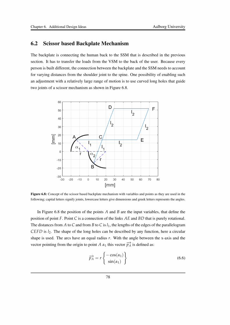
Chapter 6. Additional Design Ideas Aalborg University
6.2 Scissor based Backplate Mechanism
The backplate is connecting the human back to the SSM that is described in the previous
section. It has to transfer the loads from the VSM to the back of the user. Because every
person is built different, the connection between the backplate and the SSM needs to account
for varying distances from the shoulder joint to the spine. One possibility of enabling such
an adjustment with a relatively large range of motion is to use curved long holes that guide
two joints of a scissor mechanism as shown in Figure 6.8.
Figure 6.8: Concept of the scissor based backplate mechanism with variables and points as they are used in the
following; capital letters signify joints, lowercase letters give dimensions and greek letters represents the angles.
In Figure 6.8 the position of the points A and B are the input variables, that define the
position of point F. Point C is a connection of the links AE and BD that is purely rotational.
The distances from A to C and from B to C is l1, the lengths of the edges of the parallelogram
CEFD is l2. The shape of the long holes can be described by any function, here a circular
shape is used. The arcs have an equal radius r. With the angle between the x-axis and the
vector pointing from the origin to point A α1 this vector −→pA is defined as:
−→pA = r
{− cos(α1)
sin(α1)
}(6.6)
78
Chapter 6. Additional Design Ideas Aalborg University
In a similar manner the vector from the origin to the point B −→pB is
−→pB = r
{1− cos α2
− sin α2
}(6.7)
The connecting vector of those two points will be called −→pAB and is given by:
−→pAB = −→pB −−→pA (6.8)
Together with the vector from point A to point C, −→pAC, and the vector from B to C, −→pBC,−→pAB creates an isosceles triangle. The angle between −→pAB and −→pBC is
γ = 2 arcsin
(∣∣−→pAB∣∣
2l1
)(6.9)
To obtain the position of C, a vector is needed that is perpendicular to −→pAB to construct a
right-angle triangle. With such a triangle the known length l1 and the known angle γ can be
used to calculate the vector from the origin to C, −→pC:
−→pC = −→pA + 0.5−→pAB +1∣∣−→pAB∣∣{−pAB 2
pAB 1
}l1 cos
(γ
2
)(6.10)
Here the notation −−→pAB i describes the ith element of the vector −→pAB. Because the links of the
parallelogram CEFD are of equal length and the angle between the links at C is known, the
position of the endpoint F is calculated as vector −→pF from the origin to F:
−→pF = −→pC +1∣∣−→pAB∣∣{−pAB 2
pAB 1
}l2 cos
(γ
2
)(6.11)
Because the links AE and BD are rigid and only connected in C but not interrupted, the
corresponding position vectors are found to be
−→pD = −→pC + l2−→pBC∣∣−→pBC
∣∣ = −→pC +l2l1−→pBC (6.12)
−→pE = −→pC + l2−→pAC∣∣−→pAC
∣∣ = −→pC +l2l1−→pAC (6.13)
The vectors −→pAC and −→pBC that have been used have the length l1 and are obtained from −→pA,−→pB and −→pC.
−→pAC = −→pC −−→pA (6.14)−→pBC = −→pC −−→pB (6.15)
79

Chapter 6. Additional Design Ideas Aalborg University
With the geometry of this idea fully described, a MATLAB script has been used to plot
a variety of the points that F can take. Table 6.1 lists the variables that have been used for
Figure 6.8 and Figure 6.9. In Figure 6.9, the black arcs signify the curved long holes, in
which the points A and B slide. The blue areas are points, that F can take. In Figure 6.9a
both long holes reach from 0◦ to 90◦. The result is a range of motion that is more circular
than stretched in a diagonal direction. If the second angle α2 is increased to range from 0◦ to
180◦ as depicted in 6.9b, an extension to the shape from 6.9a in the direction of the origin is
added. In a real-life application, it would not be possible to have zero distance between −→pAB
and F, but F can be made to touch the x-axis by extending α1 into the negative region of its
definition.
The influence of the different variables of the system on the shape of the possible motion
is not obtained intuitively. As can be seen in Figure 6.9c, the range of motion might include
areas that cannot be reached, although they are surrounded by reachable points. For the task
at hand, an extended diagonal of the shape zm = mxm where m is an arbitrary positive
number and zm and xm are axes in the bodies reference coordinate system as introduced in
Section 3.1, might be a desirable shape of the range of motion of F. However, to optimise
the variables of the system towards such a shape is not a trivial task, as an objective function
that accounts for holes in the range of motion is not easily found. It is also questionable if
a circular shape of the long holes is the best possible solution since any arbitrary function,
even discontinuous ones, are possible. Figure 6.9d shows an educated guess of what might
be a good solution for the requirement of the extended diagonal of the shape zm.
Variable Value
l1 30mml2 40mmr 20mm
Table 6.1: Input variables for the figures of this section
80

Chapter 6. Additional Design Ideas Aalborg University
(a) (b)
(c) (d)
Figure 6.9: Range of motion for various ranges of α1 and α2 with the remaining variables as listed in Table
6.1; the angles are incremented with 1◦
(a) α1 = 0◦...90◦ and α2 = 0◦...90◦
(b) α1 = 0◦...90◦ and α2 = 0◦...180◦
(c) α1 = 0◦...180◦ and α2 = 0◦...180◦
(d) α1 = 45◦...120◦ and α2 = 120◦...180◦
This scissor based backplate mechanism provides an approach to account for different
distances of the shoulder joint to the spine. It can be adapted for the curvature of the human
back by transferring the system to a sphere with a smaller than the indefinite radius. It has the
advantage, that with only two screws a relatively wide range of motion is covered, but needs
further investigation regarding the shape of the long holes, the dimensions of the different
variables and the remaining stiffness of the backplate and the system itself. Since the main
objective of the project is the design of a passive exoskeleton that provides assistance with
the motion of the shoulder, this approach is not followed.
81
Chapter 7
Preliminary Test of the Exoskeleton
In this chapter the test of the exoskeleton is described. First the range of motion and the
limitations of the exoskeleton are examined. After this, the torque that the included VSM can
provide is tested and is compared with the analytical and numerical analyses. The conclu-
sions of the test of the exoskeleton are discussed, which also includes possible improvements.
In the end of the chapter, a discussion is made regarding the design process with focus on
the problem definition.
7.1 Testing of the Exoskeleton
In order to test the exoskeleton, the Range of Motion (RoM) needs to be examined. To do so,
the SSM is attached to a backplate. The backplate used is an already existing one from the
AAU laboratory. It is mounted to a wheelchair, so the testing person has to sit and position
itself relative to the shoulder mechanism instead of the shoulder mechanism being attached
to the body.
In order to validate the results of the analytical and numerical analyses, the torque of the
exoskeleton is examined. Due to lack of time and the corona situation, the exoskeleton was
examined only by the authors, so the results might not be representative.
7.2 Range of Motion
To examine the range of motion the exoskeleton is attached to the arm in the Outer Frame
and a backplate in one end of the SSM. The backplate is attached to a wheelchair to be stable
so there was no need to connect the user and the backplate by straps. Furthermore, it has to
82
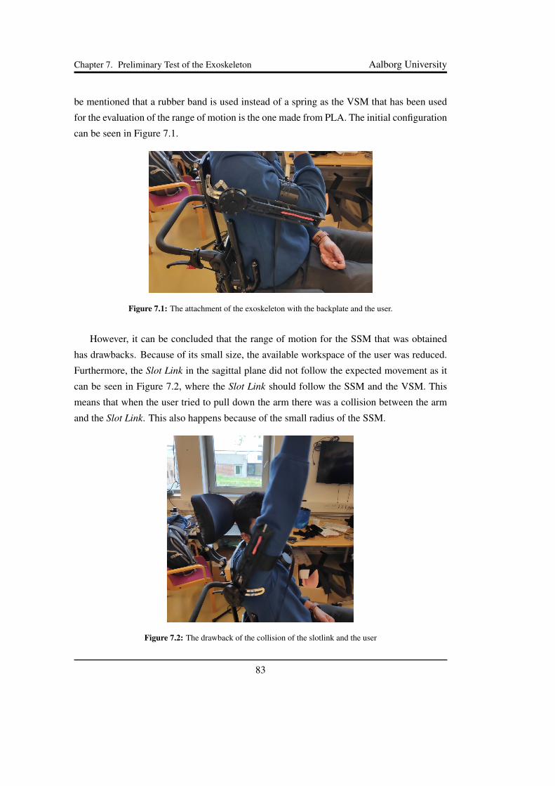
Chapter 7. Preliminary Test of the Exoskeleton Aalborg University
be mentioned that a rubber band is used instead of a spring as the VSM that has been used
for the evaluation of the range of motion is the one made from PLA. The initial configuration
can be seen in Figure 7.1.
Figure 7.1: The attachment of the exoskeleton with the backplate and the user.
However, it can be concluded that the range of motion for the SSM that was obtained
has drawbacks. Because of its small size, the available workspace of the user was reduced.
Furthermore, the Slot Link in the sagittal plane did not follow the expected movement as it
can be seen in Figure 7.2, where the Slot Link should follow the SSM and the VSM. This
means that when the user tried to pull down the arm there was a collision between the arm
and the Slot Link. This also happens because of the small radius of the SSM.
Figure 7.2: The drawback of the collision of the slotlink and the user
83
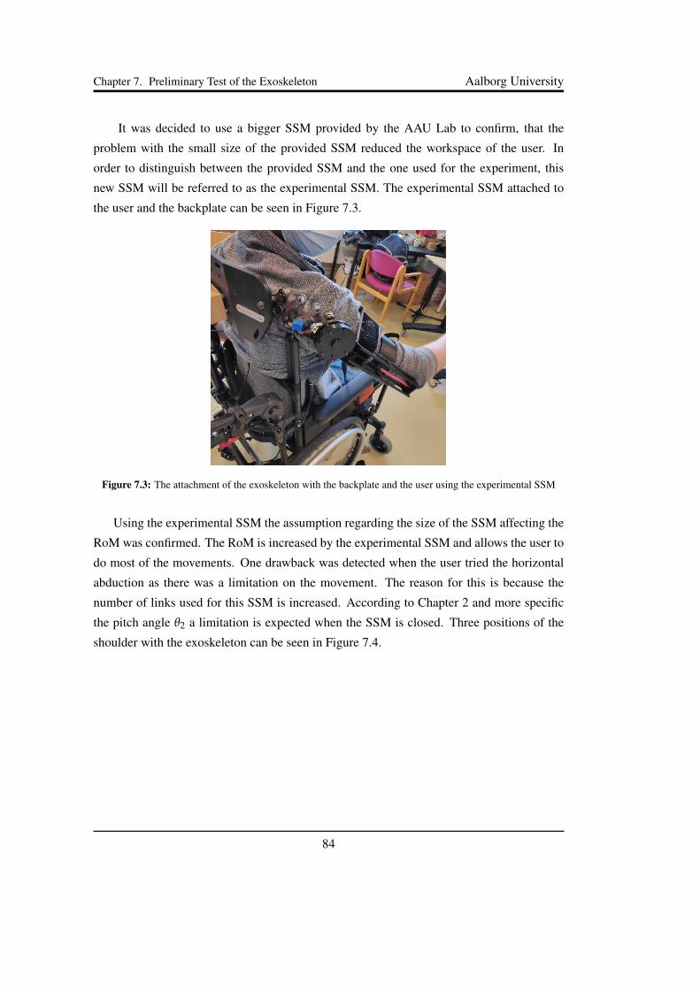
Chapter 7. Preliminary Test of the Exoskeleton Aalborg University
It was decided to use a bigger SSM provided by the AAU Lab to confirm, that the
problem with the small size of the provided SSM reduced the workspace of the user. In
order to distinguish between the provided SSM and the one used for the experiment, this
new SSM will be referred to as the experimental SSM. The experimental SSM attached to
the user and the backplate can be seen in Figure 7.3.
Figure 7.3: The attachment of the exoskeleton with the backplate and the user using the experimental SSM
Using the experimental SSM the assumption regarding the size of the SSM affecting the
RoM was confirmed. The RoM is increased by the experimental SSM and allows the user to
do most of the movements. One drawback was detected when the user tried the horizontal
abduction as there was a limitation on the movement. The reason for this is because the
number of links used for this SSM is increased. According to Chapter 2 and more specific
the pitch angle θ2 a limitation is expected when the SSM is closed. Three positions of the
shoulder with the exoskeleton can be seen in Figure 7.4.
84

Chapter 7. Preliminary Test of the Exoskeleton Aalborg University
(a) (b)
(c)
Figure 7.4: Three motions of the shoulder with the exoskeleton, (a) flexion, (b) horizontal adduction and (c)
horizontal abduction
7.2.1 Measurement of the RoM
In order to measure the RoM of the exoskeleton, the three main planes are examined. These
planes are described in Chapter 1 and are the sagittal, the coronal and the transverse planes.
The widely accepted method of measuring the range of motion of joints is the usage of go-
niometers, but it has been shown that the smartphone application "Clinometer" from Plain-
code Software Solutions also gives acceptable measurements [Werner et al., 2013]. The
measurements are done using a protractor for the transverse plane and the Clinometer for
85
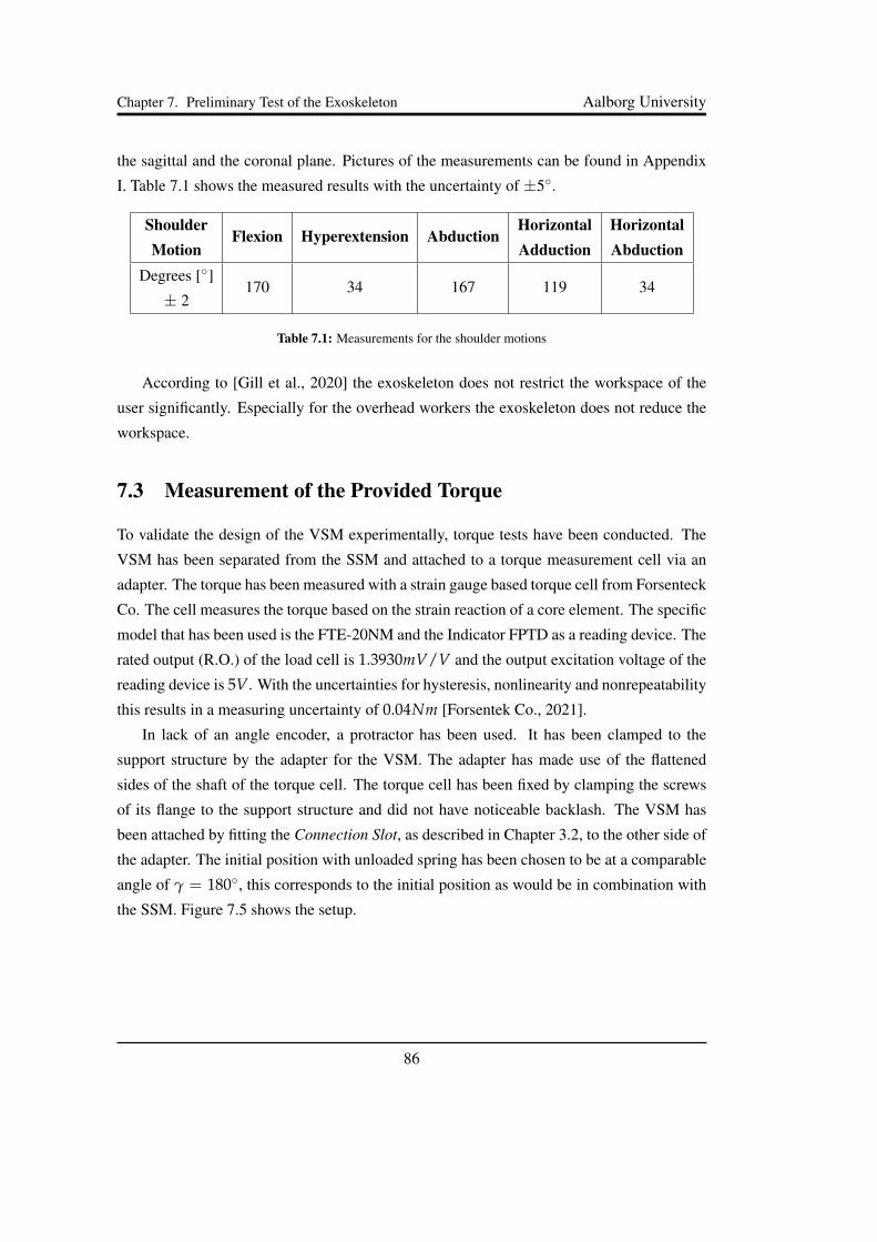
Chapter 7. Preliminary Test of the Exoskeleton Aalborg University
the sagittal and the coronal plane. Pictures of the measurements can be found in Appendix
I. Table 7.1 shows the measured results with the uncertainty of ±5◦.
ShoulderMotion
Flexion Hyperextension AbductionHorizontalAdduction
HorizontalAbduction
Degrees [◦]
± 2170 34 167 119 34
Table 7.1: Measurements for the shoulder motions
According to [Gill et al., 2020] the exoskeleton does not restrict the workspace of the
user significantly. Especially for the overhead workers the exoskeleton does not reduce the
workspace.
7.3 Measurement of the Provided Torque
To validate the design of the VSM experimentally, torque tests have been conducted. The
VSM has been separated from the SSM and attached to a torque measurement cell via an
adapter. The torque has been measured with a strain gauge based torque cell from Forsenteck
Co. The cell measures the torque based on the strain reaction of a core element. The specific
model that has been used is the FTE-20NM and the Indicator FPTD as a reading device. The
rated output (R.O.) of the load cell is 1.3930mV/V and the output excitation voltage of the
reading device is 5V. With the uncertainties for hysteresis, nonlinearity and nonrepeatability
this results in a measuring uncertainty of 0.04Nm [Forsentek Co., 2021].
In lack of an angle encoder, a protractor has been used. It has been clamped to the
support structure by the adapter for the VSM. The adapter has made use of the flattened
sides of the shaft of the torque cell. The torque cell has been fixed by clamping the screws
of its flange to the support structure and did not have noticeable backlash. The VSM has
been attached by fitting the Connection Slot, as described in Chapter 3.2, to the other side of
the adapter. The initial position with unloaded spring has been chosen to be at a comparable
angle of γ = 180◦, this corresponds to the initial position as would be in combination with
the SSM. Figure 7.5 shows the setup.
86

Chapter 7. Preliminary Test of the Exoskeleton Aalborg University
(a) (b)
Figure 7.5: (a) clamping of the protractor, (b) VSM attached in unloaded position with the torque cell in the
background in blue
Measurements have been conducted with two setups. The first setup used 3D printed
pulleys running on screws. Those results will not be presented here but can be seen in
Appendix J, because the high friction between the pulleys and the screws caused a large
hysteresis with a maximum torque of around 300% of the predicted value. Instead, the
results that are presented have been obtained after replacing the 3D printed pulleys with
metal pulleys that run on roller bearings. Those are of the same outer radius, but the radius
that the cable runs in is 0.5mm smaller in diameter.
Various measurements with different spring stiffnesses have been conducted. The first
spring that the VSM has been tested with had a stiffness of 0.84N/mm. The results were
used to improve the measurement procedure and can be seen in Appendix K. The measure-
ments, that are presented in Figure 7.6, have been conducted with a spring with a stiffness of
3.52N/mm and a preload of 27.18N. The mechanism has been rotated to a certain angle by
one person and two other persons noted the torque value independently of each other. Before
saving the value, it has been waited for the reading to settle. Three cycles have been con-
ducted where the angle increment of which readings were taken was 5◦. One cycle consists
of 180◦ where the torque was measured during loading and unloading. At 180◦ two readings
have been taken, the first one when coming from 175◦ and the second one after ensuring a
stable position of 180◦. After each cycle, the cable has been tightened to eliminate backlash
even at small deflections.
87

Chapter 7. Preliminary Test of the Exoskeleton Aalborg University
Figure 7.6: Average and standard derivation of the measured torque values over γ for the loading and the
unloading of the spring as well as the result from the analytical model and the MSC ADAMS simulation
Figure 7.6 shows the average values of the torque readings where all readings have the
same weight, so they are interpreted as independent cycles. Each phase is represented by the
average value and the standard deviation of the torque readings. At points of the curve where
no standard deviation is given, the curve is interpolated and no measurements have been
conducted. The highest standard deviation is 0.38Nm and is observed during the loading of
the spring at an angle of γ = 125◦. A figure with the measured data points can be found in
Appendix L.
It can be observed, that from the start of the cycle the measured torque aligns well with
the predictions, although it meanders around both, the analytical and the simulated predic-
tion. With γ approaching 90◦, the experimental results seem to follow more the analytical
model, which gives higher results. At γ = 90◦ the experimental results detach from the
predicted results and while over the following 35◦ to 40◦ the predicted torque decreases,
the measured torque remains almost constant with a peak at γ = 55◦. From the constant
section on, the experimentally obtained torque decreases and shows a similar slope to the
predicted curves. At γ = 0◦ after 180◦ deflection, a torque discrepancy of 1.9Nm between
the predictions and the readings remains.
At the beginning of the unloading phase at γ = 0◦ the measured torque aligns with the
predictions. For the first 15◦ to 20◦ of the motion, the torque is negative, but shows a sim-
ilar slope to the predictions and the loading phase until γ = 35◦. In this area, the standard
deviation shows larger values than in the rest of the unloading curve with the maximum of
88
Chapter 7. Preliminary Test of the Exoskeleton Aalborg University
0.25Nm at γ = 35◦. From there on with increasing γ the slope is more flat-angled than
the predictions, although the position of the maximum of the unloading phase aligns with
the predicted curves. From the maximum on, the torque diminishes with different slope than
before until zero torque is reached at γ = 165◦ or 15◦ deflection from the initial angle.
Conclusions
The begin of the cycle shows very good alignment between the experimental results and the
predictions. This is expected as the validity of the analytical model has been shown prior [Li
et al., 2020], [Bai & Li, 2019]. The detaching after 90◦ can be a result of increasing friction.
When the spring gets elongated, the cable force increases, thus adding force on the bearings.
Because the VSM has been moved by hand in increments, this friction has to be overcome
for every increment. It is seen that the difference increases from increment to increment in
the range of γ = 90◦... ∼ 35◦, after which the deviation stays constant. In the unloading
phase it can be concluded from looking at the average of the loading and unloading curves in
the range of γ = 15◦...35◦, that the same difference acting in opposite direction is causing
the hysteresis. This makes the deviation likely to be produced by friction in the bearings.
The used bearings are gliding bearings and the gliding surfaces are not perfect. Thus the two
surfaces produce more and more friction with increasing cable force, until the maximum
amount of friction that can be produced is reached, which leads to the hysteresis that is
observed. This theory could be confirmed by further experiments where the temperature in
the bearing is measured or where the bearings are exchanged for a roller bearings and the
results are compared to the results with the present gliding bearings.
At the start of the unloading phase, the measured torque is negative and free motion is
not possible. After overcoming the area where the friction is constricting the motion, the
standard deviation is in the largest region between γ = 15◦...45◦. Directly after this region,
the slope of the curve changes abruptly, causing a deviation of the average of the loading and
unloading from the predictions. Compared to the predicted curves and the loading phase,
the slope is now more flat. Because of the high standard deviation of the readings, the slope
decoupling, the lower maximum and the fact, that zero torque is reached at a larger than zero
deflection, it is assumed, that in the area of γ = 15◦...45◦ the cable is irreversibly elongated,
leading to a smaller force and reaching zero torque prior to zero deflection. In Li et al. [2020]
a similar effect is observed and explained by nonlinearity of the cable and manufacturing
imperfections. It is assumed here, that with a constant cable length, the hysteresis shown
should decrease and the average of the loading and the unloading process should follow the
89

Chapter 7. Preliminary Test of the Exoskeleton Aalborg University
predicted torque curve more closely.
7.4 Future Work
In this section improvements and remaining work for the further development of the current
design are described. Those are derived from the preliminary testing of the exoskeleton and
general reflection on the prototype.
7.4.1 General Improvements
In the following, some ideas to improve the design, as well as detected shortcomings, are
listed. Those could not be implemented or improved, respectively, due to the limited amount
of time.
• One drawback that has been detected during the experiment for the range of motion
concerns the straps that connect the VSM with the user’s arm. Since there was only
one location assigned on the VSM for connection of the strap, the VSM was not stable.
As a result, the whole exoskeleton failed to align properly when the arm was moved.
However, when two pairs of straps were used the VSM was more stable and aligned
better with the arm.
• During the measurements of the torque provided by the VSM, it was found that there
was high friction, which caused a large hysteresis. By switching to pulleys with roller
bearings the problem was reduced slightly. To reduce friction further, the design of
the housing has to be changed to use roller bearings instead of polymer sleeve bear-
ings. In the literature, the use of double-row roller bearings with large safety factors
to reduce internal forces is recommended [Dežman & Gams, 2018]. This approach
has not been followed to enable a compact design.
• There are a couple of minor issues with the design of the housing of the prototype, too.
The first one is, that the Outer Housing is pressed against the pulleys by the screws.
This compromises the rotation of the pulleys due to an increase in the friction between
the contact surfaces. This problem can be overcome by adding spacers between the
Outer Housing and the Outer Frame. Also for long term usage of the mechanism, the
housing should be enclosed to protect it from dust entering, as this again will increase
90
Chapter 7. Preliminary Test of the Exoskeleton Aalborg University
the friction.
• During the experiment, it proved to be vital for the function, that the joints of the SSM
are aligned with the glenohumeral joint of the test person. This calls for a flexible
and well adjustable backplate, that is capable of easily customizing the position of
the common joint of the backplate and the SSM. A further improvement would be to
give the backplate the range of motion to follow the shoulder in the two translational
degrees of freedom as well.
• To further improve the user experience, the Connetion Slot should contain rollers. This
will make it easier for the user to force the axis of rotation of the VSM to follow the
arm.
• So far no thought has been given to the weight of the assembly. During the experiment,
it has been observed, that the SSM has the tendency to rotate around the common joint
with the backplate. Stiffening this rotation not only makes the mechanism less fee-
lable but also increases the assisted range of motion as described in Section 6.1.2.
• From the torque measurement it has been concluded, that the cable length is increased
irreversibly during the usage of the mechanism. An ultimate reason could not be found
as the cable that was used is a plaited PES rope with a tensile strength of 1000N and
the maximum applied force is around one-third of the strength. For a quick solution,
a steel cable can be used, although this cannot be expected to reduce the hysteresis
completely as there are other influences like manufacturing imperfections that can
also cause hysteresis [Li et al., 2020].
• The exoskeleton is only examined by the authors of this project. In order for the
results to be more representative regarding the range of motion and the comfort of the
exoskeleton, the exoskeleton has to be examined by external users.
7.4.2 Updated Scissors Design
Since the SSM is found to be too small, it is decided to update the design and make it larger
to fit the user and cover more range of motion. Using the provided SSM design and taking
91

Chapter 7. Preliminary Test of the Exoskeleton Aalborg University
inspiration from the experimental SSM the final design of the SSM is developed and can
be seen in Figure 7.7. The final design combines the range of motion of the experimental
SSM and also the compactness of the provided SSM. The stress analysis is conducted on the
updated design in order to validate that it can withstand the torque provided by the VSM.
The dimensions of the SSM are provided in Appendix G.
Figure 7.7: Updated design of the SSM
It is decided to use Aluminium-7075 T6 for this design. The loading and boundary con-
dition of the study is similar to the one used in 5.2.1. A cylindrical fixed support is used on
one end of the Scissors and the moment of 6532Nmm is applied on the Connection Slot.
The stress distribution on the updated Scissors mechanism can be seen in Figure 7.8. It is
seen that there is a stress concentration where the boundary condition is applied. Ignoring
this and probing the sections on the links which are not under the influence of stress con-
centration, it is found that, the maximum stress is 227MPa. This value is still under the
safety limit. The result for the stress value in the links and convergence study can be seen in
Appendix F.
92
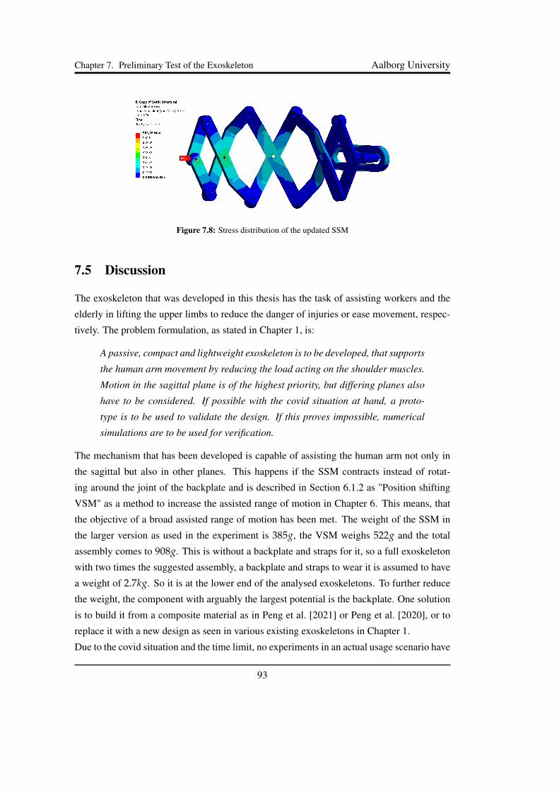
Chapter 7. Preliminary Test of the Exoskeleton Aalborg University
Figure 7.8: Stress distribution of the updated SSM
7.5 Discussion
The exoskeleton that was developed in this thesis has the task of assisting workers and the
elderly in lifting the upper limbs to reduce the danger of injuries or ease movement, respec-
tively. The problem formulation, as stated in Chapter 1, is:
A passive, compact and lightweight exoskeleton is to be developed, that supports
the human arm movement by reducing the load acting on the shoulder muscles.
Motion in the sagittal plane is of the highest priority, but differing planes also
have to be considered. If possible with the covid situation at hand, a proto-
type is to be used to validate the design. If this proves impossible, numerical
simulations are to be used for verification.
The mechanism that has been developed is capable of assisting the human arm not only in
the sagittal but also in other planes. This happens if the SSM contracts instead of rotat-
ing around the joint of the backplate and is described in Section 6.1.2 as "Position shifting
VSM" as a method to increase the assisted range of motion in Chapter 6. This means, that
the objective of a broad assisted range of motion has been met. The weight of the SSM in
the larger version as used in the experiment is 385g, the VSM weighs 522g and the total
assembly comes to 908g. This is without a backplate and straps for it, so a full exoskeleton
with two times the suggested assembly, a backplate and straps to wear it is assumed to have
a weight of 2.7kg. So it is at the lower end of the analysed exoskeletons. To further reduce
the weight, the component with arguably the largest potential is the backplate. One solution
is to build it from a composite material as in Peng et al. [2021] or Peng et al. [2020], or to
replace it with a new design as seen in various existing exoskeletons in Chapter 1.
Due to the covid situation and the time limit, no experiments in an actual usage scenario have
93
Chapter 7. Preliminary Test of the Exoskeleton Aalborg University
been conducted. This is to be done when the design improvements have been implemented.
The conducted tests have proven, that the range of motion of the original scissors is too small.
However, with the design as described in Section 7.4.2 the range of motion is deemed to be
sufficient, but more precise measurements have to be conducted. It also has been proven by
FEM analysis, that the loads from the torque providing mechanism can be sustained by the
updated scissors.
The torque tests as described in Section 7.3 revealed, that the overall design and optimisation
process has yielded a functional actuator design. It has been concluded from the experiment,
that the torque that is predicted by the analytical model of the mechanism and the MSC
ADAMS simulation can be met if certain improvements are implemented. The most impor-
tant one is the usage of a stiffer cable with less nonlinear effects. Secondly, bearings with
lower friction have to be used in order to reduce the hysteresis.
94

Chapter 8
Conclusion
In this thesis, a design of a compliant shoulder exoskeleton is presented. The recently de-
veloped Shoulder Scissors Mechanism is used to reproduce the motion of the shoulder joint
and a Variable Stiffness Mechanism is used for gravitational compensation for the human
arm.
The upper body kinematics was studied to develop the torque requirement for the VSM.
Using optimisation, the dimensions of the VSM were calculated and used to develop the
initial design of the mechanism. The loads acting on the VSM were calculated in MSC
ADAMS and used in Ansys to conduct a structural analysis of the mechanism.
Topology optimisation was used to reduce the mass of the VSM. A final design was
developed which reduced the weight of the original Outer Frame by 70% from 466g to
143g. This design was successfully confirmed to withstand the loads experienced by the
mechanism. Additional design ideas were also presented to include assistance for the second
degree of freedom in the abduction/adduction plane.
The torque generated by the VSM was experimentally measured using a torque sensor
and the result was compared with the analytical and numerical solution. It was observed
that there was a discrepancy in the readings due to the high friction experienced by the
pulleys in the VSM. The Range of Motion of the device was also measured experimentally
by connecting the exoskeleton to the backplate. The drawbacks of the mechanism were
studied and possible improvements were suggested.
Overall, the novel mechanism provides a large range of motion and is estimated to be
lighter than the most of the exoskeletons that have been studied. Its compactness, modularity
and adaptable torque behaviour make it interesting for further development.
95

Bibliography
ANSYS (2021). Mechanical user’s guide. ANSYS. Downloaded: 18-5-2021.
Bai, S. & Li, Z. (2019). A novel revolute joint of variable stiffness with reconfigurability.
Mechanism and Machine Theory, 133, 720–736.
Bai, S., Virk, G. S., & Sugar, T. (2018). Wearable Exoskeleton Systems : Design, Control and
Applications. Control, Robotics and Sensors. Institution of Engineering and Technology.
Castro, M. N., Rasmussen, J., Andersen, M. S., & Bai, S. (2019). A compact 3-dof shoulder
mechanism constructed with scissors linkages for exoskeleton applications. Mechanism
and Machine Theory, 132, 264–278.
Chen, Y., Li, G., & Zhu, Y. (2014). Design of a 6-dof upper limb rehabilitation exoskeleton
with parallel actuated joints. Bio-Medical Materials and Engineering, 24(6), 2527–2535.
Choi, H. (2018). Suitx. https://www.suitx.com/backX. Accessed: 30-05-2021.
Choi, H. (2021). Assistance of a person with muscular weakness using a a joint-torque-
assisting exoskeletal robot. Applied Sciences, 11(7).
Christensen, S. & Bai, S. (2017). A novel shoulder mechanism with a double parallelogram
linkage for upper-body exoskeletons. Biosystems and Biorobotics, 16, 51–56.
de Leva, P. (1996). Adjustment to zatsiorsky-seluyanov’s segment inertia parameters. Jour-
nal of Biomechanics, 29(9), 1223–1230.
Dežman, M. & Gams, A. (2018). Rotatable cam-based variable-ratio lever compliant actua-
tor for wearable devices. Mechanism and Machine Theory, 130, 508–522.
Exobionics (2018). Exobionics. https://eksobionics.com/past-products/.
Accessed: 05-03-2021.
96

Bibliography Aalborg University
Exobionics (2020). Evo. https://eksobionics.com/ekso-evo/. Accessed:
05-03-2021.
Farah, S., Anderson, D. G., & Langer, R. (2016). Physical and mechanical properties of
pla, and their functions in widespread applications — a comprehensive review. Advanced
Drug Delivery Reviews, 107, 367–392. PLA biodegradable polymers.
Feeney, D. (2019). 3d printing with abs vs pla. https://www.sd3d.com/3d-prin
ting-abs-vs-pla/. Accessed: 16-05-2021.
Forsentek Co., L. (2021). Static torque measurement device 20nm 10nm 5nm 2nm 1nm
measure torque. http://www.forsensor.com/sale-8832707-static-to
rque-measurement-device-20nm-10nm-5nm-2nm-1nm-measure-torq
ue.html. Accessed: 31-05-2021.
Furnémont, R., Mathijssen, G., van der Hoeven, T., Brackx, B., Lefeber, D., & Vanderborght,
B. (2015). Torsion maccepa: A novel compact compliant actuator designed around the
drive axis. In 2015 IEEE International Conference on Robotics and Automation (ICRA)
(pp. 232–237).
Gill, T. K., Shanahan, E. M., Tucker, G. R., Buchbinder, R., & Hill, C. L. (2020). Shoulder
range of movement in the general population: age and gender stratified normative data
using a community-based cohort. BMC Musculoskelet Disord, 21(1).
Gull, M. A., Bai, S., & Bak, T. (2020). A review on design of upper limb exoskeletons.
Robotics, 9(1).
Hyun, D. J., Bae, K., Kim, K., Nam, S., & hyun Lee, D. (2019). A light-weight passive upper
arm assistive exoskeleton based on multi-linkage spring-energy dissipation mechanism for
overhead tasks. Robotics and Autonomous Systems, 122, 103309.
Jafari, A., Tsagarakis, N. G., Vanderborght, B., & Caldwell, D. G. (2010). A novel ac-
tuator with adjustable stiffness (awas). In 2010 IEEE/RSJ International Conference on
Intelligent Robots and Systems (pp. 4201–4206).
Kohnke, P. (1999). Theory reference. Downloaded: 15-05-2021.
Krishnan, R., N. B., Gutierrez-Farewik, E. M., & Smith, C. (2019). A survey of human
shoulder functional kinematic representations. 57, 339–367.
97
Bibliography Aalborg University
Li, Z., Bai, S., Madsen, O., Chen, W., & Zhang, J. (2020). Design, modeling and testing of a
compact variable stiffness mechanism for exoskeletons. Mechanism and Machine Theory,
151, 103905.
Lo, H. S. & Xie, S. S. (2014). Optimization of a redundant 4r robot for a shoulder exoskele-
ton. Robotica, 32(8), 798–803.
Ltd, I. B. L. (2021). Pla vs abs. https://www.makeitfrom.com/. Accessed:
16-05-2021.
Lund, E., Olhoff, N., & Du, J. (2019). Topology optimization and its application in static
design of continuum structures. Downloaded: 25-05-2021.
Luque, E. P. (2019). Evaluation of the use of exoskeletons in the range of motion of workers.
Downloaded: 13-4-2021.
Marinov, B. (2016). Introduction to the commercial exoskeletons catalog.
https://exoskeletonreport.com/2016/12/introduction-to-the-commercial-exoskeletons-
catalog/. Accessed: 20-03-2021.
MathWorks, I. (2021a). Constrained nonlinear optimization algorithms. https://de.m
athworks.com/help/optim/ug/constrained-nonlinear-optimizat
ion-algorithms.html#brnpd5f. Accessed: 22-03-2021.
MathWorks, I. (2021b). fmincon. https://de.mathworks.com/help/optim/ug
/fmincon.html. Accessed: 22-03-2021.
MATWEB (2021). Material property data. http://www.matweb.com/index.aspx.
Accessed: 16-05-2021.
Maurice, P., Camernik, J., Gorjan, D., Schirrmeister, B., Bornmann, J., Tagliapietra, L.,
Latella, C., Pucci, D., Fritzsche, L., & Ivaldi, S. (2020). Objective and subjective effects
of a passive exoskeleton on overhead work. IEEE Transactions on Neural Systems and
Rehabilitation Engineering, 28(1), 152–164.
Mscsoftware (2010). Md adams release guide. https://www.mscsoftware.com/.
Accessed: 21-03-2021.
Naidu, M. D., Stopforth, D. R., Bright, P. G., & Davrajh, M. S. (2011). A 7 dof exoskele-
ton arm:shoulder,elbow,wrist and hand mechanism for assistance to upper limb disabled
individuals. Computer Science, (pp. 1–6).
98
Bibliography Aalborg University
Nobel-Jørgensen, M. (2016). Interactive Topology Optimization. PhD thesis.
Norton, R. L. (2010). Machine Design - An Integrated Approach, volume 4. Prentice Hall.
Pacifico, I. & Scano, A. (2020). An experimental evaluation of the proto-mate: A novel
ergonomic upper-limb exoskeleton to reduce workers’ physical strain. IEEE Robotics
Automation Magazine, 27(1), 54–65.
Paexo (2018). Paexo. https://paexo.com/paexo-shoulder/. Accessed: 05-03-
2021.
Palais, B., Palais, R., & Rodi, S. (2009). A disorienting look at euler’s theorem on the axis
of a rotation. The American Mathematical Monthly, 116(10), 892–909.
Papadopoulos, E. & Patsianis, G. (2007). Design of an exoskeleton mechanism for the
shoulder joint. IFToMM.
Peng, X., Dai, Z., Liu, J., & Wang, Q. (2020). The design and calculation of the exoskeleton
backplate based on the composite sandwich structure. IOP Conference Series: Earth and
Environmental Science, 571, 012118.
Peng, X., Dai, Z., Liu, J., & Wang, Q. (2021). Design and simulation of sandwich structure
of exoskeleton backplatebased on biological inspiration. Journal of Physics: Conference
Series, 1885.
Sigmund, O. (2001). A 99 line topology optimization code written in matlab. Structural and
Multidisciplinary Optimization, 21, 120–127.
Soames, R., Palastanga, N., & Field, D. (1994). Anatomy and human Movement - structure
and function. Butterworth-Heinemann, second edition edition.
Sotola, M., Marsalek, P., Rybansky, D., Fusek, M., & Gabriel, D. (2021). Sensitivity analysis
of key formulations of topology optimization on an example of cantilever bending beam.
Symmetry, 13(4).
S.p.A., C. (2021). Mate-xt fit for workers. https://mate.comau.com/. Accessed:
21-02-2021.
Tim Bosch, J. v. E., Knitel, K., & de Looze, M. (2016). The effects of a passive exoskeleton
on muscle activity, discomfort and endurance time in forward bending work. Applied
ergonomics, 54, 212–217.
99

Bibliography Aalborg University
Vahrenkamp, N., Asfour, T., Metta, G., Sandini, G., & Dillmann, R. (2012). Manipula-
bility analysis. In 2012 12th IEEE-RAS International Conference on Humanoid Robots
(Humanoids 2012) (pp. 568–573).
Van Ham, R., Vanderborght, B., Van Damme, M., Verrelst, B., & Lefeber, D. (2007). Mac-
cepa, the mechanically adjustable compliance and controllable equilibrium position actu-
ator: Design and implementation in a biped robot. Robotics and Autonomous Systems,
55(10), 761–768.
Vanderborght, B., Tsagarakis, N. G., Semini, C., Van Ham, R., & Caldwell, D. G. (2009).
Maccepa 2.0: Adjustable compliant actuator with stiffening characteristic for energy effi-
cient hopping. In 2009 IEEE International Conference on Robotics and Automation (pp.
544–549).
Werner, B. C., Kuenze, C. M., Griffin, J. W., Lyons, M. L., Hart, J. M., & Brockmeier, S. F.
(2013). Shoulder range of motion: Validation of an innovative measurement method using
a smartphone. Orthopaedic Journal of Sports Medicine, 1(4_suppl), 2325967113S00106.
Wolf, S., Eiberger, O., & Hirzinger, G. (2011). The dlr fsj: Energy based design of a variable
stiffness joint. In 2011 IEEE International Conference on Robotics and Automation (pp.
5082–5089).
Wolf, S. & Hirzinger, G. (2008). A new variable stiffness design: Matching requirements
of the next robot generation. In 2008 IEEE International Conference on Robotics and
Automation (pp. 1741–1746).
Yatsun, A. & Jatsun, S. (2018). Investigation of human cargo handling in industrial ex-
oskeleton. In 2018 Global Smart Industry Conference (GloSIC) (pp. 1–5).
Zhang, Z.-Q., Wong, W.-C., & Wu, J.-K. (2011). Ubiquitous human upper-limb motion
estimationusing wearable sensors. IEEE Transactions on Information Technology in
Biomedicine, 15(4), 513–521.
100
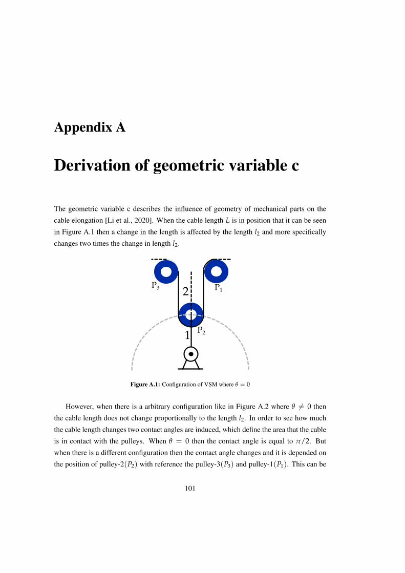
Appendix A
Derivation of geometric variable c
The geometric variable c describes the influence of geometry of mechanical parts on the
cable elongation [Li et al., 2020]. When the cable length L is in position that it can be seen
in Figure A.1 then a change in the length is affected by the length l2 and more specifically
changes two times the change in length l2.
1
2
P2
P3 P1
Figure A.1: Configuration of VSM where θ = 0
However, when there is a arbitrary configuration like in Figure A.2 where θ 6= 0 then
the cable length does not change proportionally to the length l2. In order to see how much
the cable length changes two contact angles are induced, which define the area that the cable
is in contact with the pulleys. When θ = 0 then the contact angle is equal to π/2. But
when there is a different configuration then the contact angle changes and it is depended on
the position of pulley-2(P2) with reference the pulley-3(P3) and pulley-1(P1). This can be
101
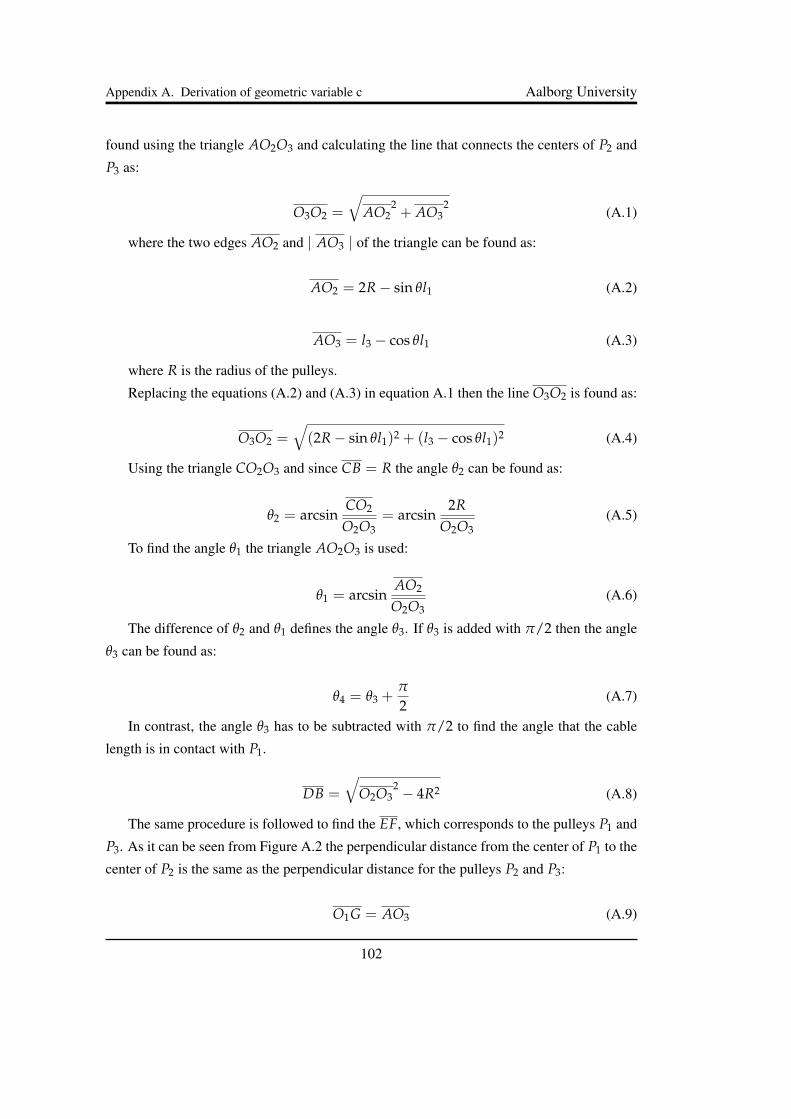
Appendix A. Derivation of geometric variable c Aalborg University
found using the triangle AO2O3 and calculating the line that connects the centers of P2 and
P3 as:
O3O2 =
√AO2
2+ AO3
2(A.1)
where the two edges AO2 and | AO3 | of the triangle can be found as:
AO2 = 2R− sin θl1 (A.2)
AO3 = l3 − cos θl1 (A.3)
where R is the radius of the pulleys.
Replacing the equations (A.2) and (A.3) in equation A.1 then the line O3O2 is found as:
O3O2 =√(2R− sin θl1)2 + (l3 − cos θl1)2 (A.4)
Using the triangle CO2O3 and since CB = R the angle θ2 can be found as:
θ2 = arcsinCO2
O2O3= arcsin
2RO2O3
(A.5)
To find the angle θ1 the triangle AO2O3 is used:
θ1 = arcsinAO2
O2O3(A.6)
The difference of θ2 and θ1 defines the angle θ3. If θ3 is added with π/2 then the angle
θ3 can be found as:
θ4 = θ3 +π
2(A.7)
In contrast, the angle θ3 has to be subtracted with π/2 to find the angle that the cable
length is in contact with P1.
DB =
√O2O3
2 − 4R2 (A.8)
The same procedure is followed to find the EF, which corresponds to the pulleys P1 and
P3. As it can be seen from Figure A.2 the perpendicular distance from the center of P1 to the
center of P2 is the same as the perpendicular distance for the pulleys P2 and P3:
O1G = AO3 (A.9)
102

Appendix A. Derivation of geometric variable c Aalborg University
Regarding the horizontal distance (O2G), it can be found as:
O2G = 2R + sin θl1 (A.10)
Using the triangle O1GO2 then the edge O2O1 can be found as:
O2O1 =
√GO1
2+ GO2
2(A.11)
The distance EF can now be found as:
EF =
√O2O1
2 − 4R2 (A.12)
on is found as:
1
32
O3
O2AB
C
D
θ1
θ2
θ
θ4
θ3
P2
P3 P1
θ1θ2
P1
P2
E
F
P3
P2
O2
O1
G
Figure A.2: An arbitary configuration of VSM where θ 6= 0.
The cable length La in an arbitrary configuration and the cable length in L when theta =
0 can be found as:
La = Rθ4 + DB + πR + EF + R(π/2− θ3) (A.13)
L = Rπ
2+ DB + Rπ + EF + R
π
2(A.14)
The geometric variable is defined as the change in the cable because of the change in
length of l2:
c =La − Ll2a − l2
(A.15)
103

Appendix A. Derivation of geometric variable c Aalborg University
where l2a is the length of link-2 in an arbitrary position.
In Figure A.3 it can be seen how the geometric variable c varies as a function of θ. It can
be concluded that the value of the geometric variable is close to 2 for the range 0◦ − 180◦ of
θ.
Figure A.3: The geometric variable c as a function of the angle θ.
104

Appendix B
Manipulator Jacobian matrix
The angular velocity ωe of the end-effector of the scissors is given from the equation below:
ωe = Jθ (B.1)
where J is the Jacobian matrix and θ are the mechanism’s joint velocities.
In geometry, Euler’s rotation theorem states that, in three-dimensional space, any dis-
placement of a rigid body such that a point on the rigid body remains fixed, is equivalent
to a single rotation about some axis that runs through the fixed point [Palais et al., 2009].
Assuming the speed of rotation θs about the instantaneous axis of rotation e then the angular
velocities ωe at any time are given as:
ωe = ˙θs e (B.2)
Based on the above equation, the angular velocities ωe can be derived from the skew-
symmetric matrix S of the angular-velocities for the particular rotation matrix Re of the
mechanism [Castro et al., 2019]. The skew-symmetric matrix S is dervided as:
S = ReRTe =
0 −ωz ωy
ωz 0 −ωx
−ωy ωx 0
(B.3)
From the above equation the three following equations can be derived:
ωx = r31r21 + r32r22 + r33r23 (B.4)
105

Appendix B. Manipulator Jacobian matrix Aalborg University
ωy = r11r31 + r12r32 + r13r33 (B.5)
ωz = r21r11 + r22r12 + r23r13 (B.6)
Replacing these thee equations in equation (B.2) for ωe = [ωx, ωy, ωz]T then the ma-
nipulator Jacobian matrix can be found as:
J =
0 cθ1 sθ1sθ2
0 sθ1 −cθ1sθ2
1 0 cθ2
(B.7)
106

Appendix C
Scissors bearings
The bearings that are used in the scissors are IGUS GFM − 0607 − 024. They are put
inside the holes of the links in order to reduce the friction of the bolts with the links. IGUS
GTM− 0611− 010 are out above the hole links in order to reduce the friction between the
head of the bolts and the links. The material of the two bearings is iglidur and are made
by high-performance polymers. Their special composition makes them extremely wear-
resistant, robust and self-lubricating.
(a)(b)
Figure C.1: The two types of bearings that used in the scissors. a) is the IGUS GFM− 0607− 024 and b) the
IGUS GTM− 0611− 010 type.
107

Appendix D
Homogeneous Matrices of the HumanArm
In the following the homogeneous matrices of the model of the human arm as described in
Section 3.1 are given. The indexing is done in such a way, that the lower index refers to the
original coordinate system and the upper index refers to the coordinate system that a point
is transferred to. The sine and cosine functions are abbreviated with si and ci respectively,
where i is the index of the coordinate system as shown in Figure 3.1b. For the transformation
108
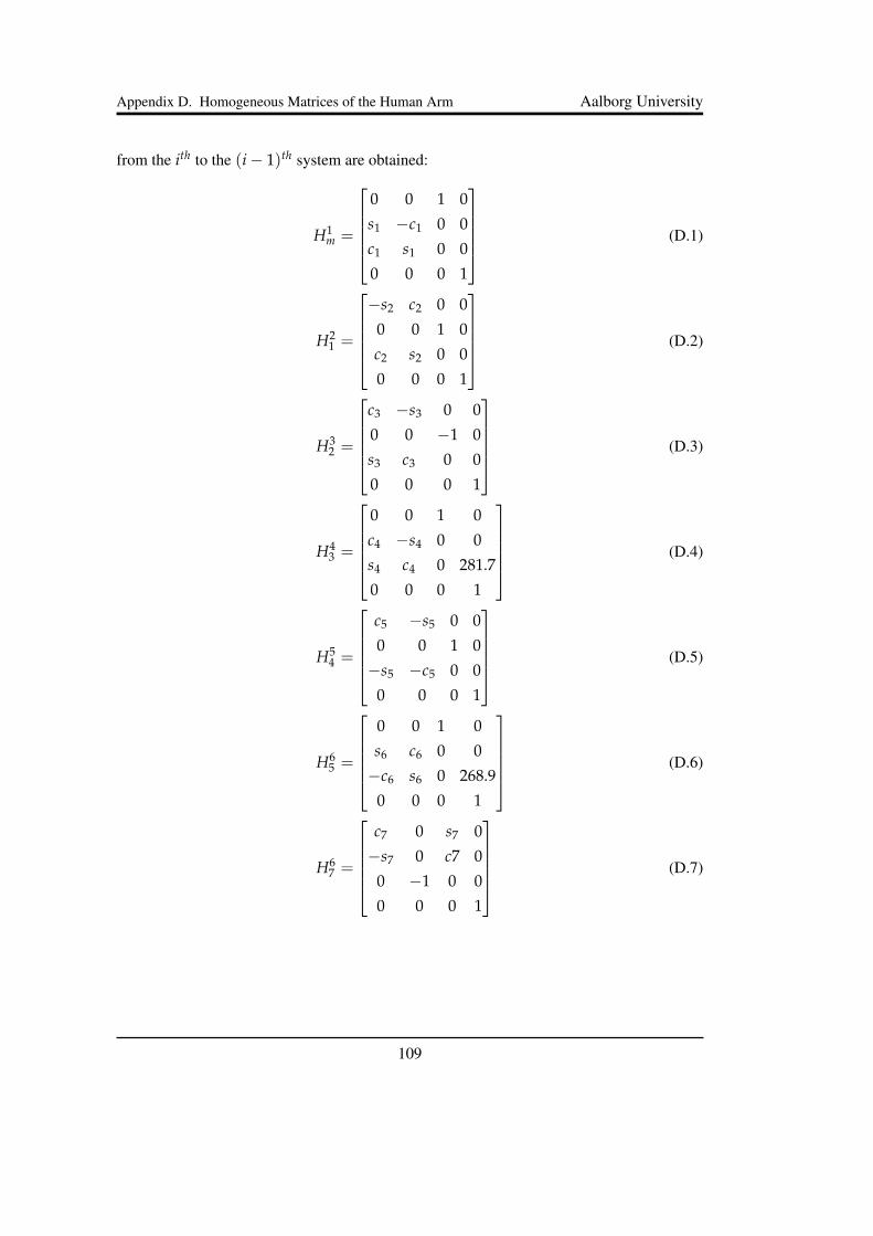
Appendix D. Homogeneous Matrices of the Human Arm Aalborg University
from the ith to the (i− 1)th system are obtained:
H1m =
0 0 1 0
s1 −c1 0 0
c1 s1 0 0
0 0 0 1
(D.1)
H21 =
−s2 c2 0 0
0 0 1 0
c2 s2 0 0
0 0 0 1
(D.2)
H32 =
c3 −s3 0 0
0 0 −1 0
s3 c3 0 0
0 0 0 1
(D.3)
H43 =
0 0 1 0
c4 −s4 0 0
s4 c4 0 281.7
0 0 0 1
(D.4)
H54 =
c5 −s5 0 0
0 0 1 0
−s5 −c5 0 0
0 0 0 1
(D.5)
H65 =
0 0 1 0
s6 c6 0 0
−c6 s6 0 268.9
0 0 0 1
(D.6)
H67 =
c7 0 s7 0
−s7 0 c7 0
0 −1 0 0
0 0 0 1
(D.7)
109

Appendix E
Pendulum example in Adams
Assuming a simple pendulum as it can be seen in figure E.1. The pendulum is attached
to a fixed frame through a revolute joint that allows the pendulum to rotate. The vector−→A represent the location of the revolute joint in the fixed reference frame, the vector
−→R
represents the location of the center of the mass of the pendulum in the fixed reference
frame and the vector −→r the distance from the center of the mass of the pendulum to the
revolute joint.
Ground
Joint
(x,y)
x
y
θ
A
Rr
Figure E.1: Simple pendulum that is attached to a fixed frame through a revolut joint..
ADAMS solver is using the Lagrange equation as it was described in equation (4.4). The
110
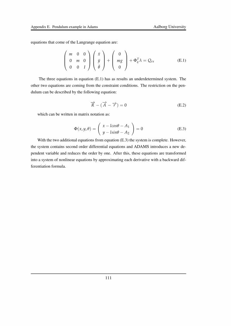
Appendix E. Pendulum example in Adams Aalborg University
equations that come of the Langrange equation are:m 0 0
0 m 0
0 0 I
xyθ
+
0
mg0
+ ΦTq λ = Qex (E.1)
The three equations in equation (E.1) has as results an underdetermined system. The
other two equations are coming from the constraint conditions. The restriction on the pen-
dulum can be described by the following equation:
−→R − (
−→A −−→r ) = 0 (E.2)
which can be written in matrix notation as:
Φ(x, y, θ) =
(x− lcosθ − A1
y− lsinθ − A2
)= 0 (E.3)
With the two additional equations from equation (E.3) the system is complete. However,
the system contains second order differential equations and ADAMS introduces a new de-
pendent variable and reduces the order by one. After this, these equations are transformed
into a system of nonlinear equations by approximating each derivative with a backward dif-
ferentiation formula.
111

Appendix F
Convergence Plots
F.1 Convergence plots for Open-Scissors
The convergence is done for the half torque provided (6532Nmm) and also for the weak
spring that used where the maximum torque was 1912 Nmm.
112

Appendix F. Convergence Plots Aalborg University
F.1.1 Stress for Torque-6532 Nmm
Figure F.1: Stress convergence study of Open-Scissors configuration for different links.
113
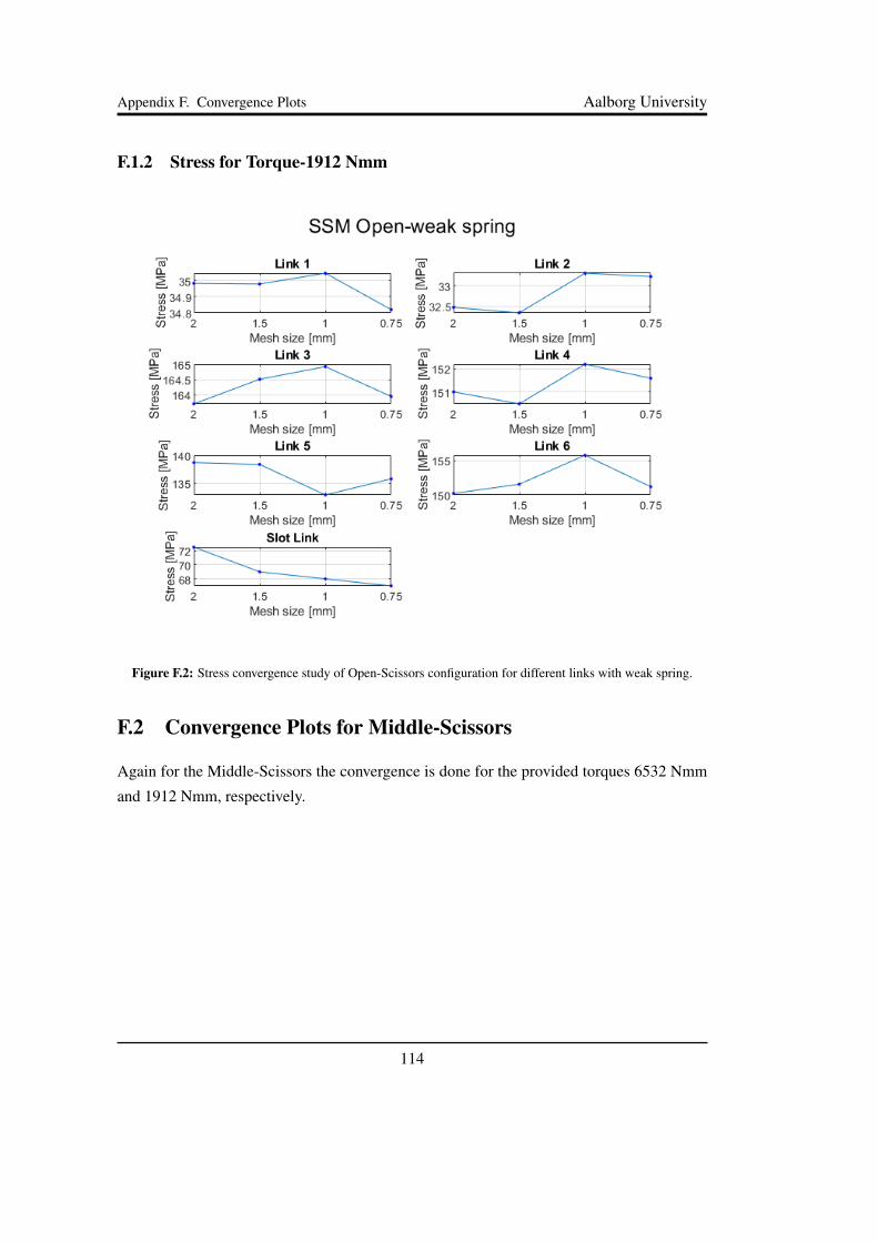
Appendix F. Convergence Plots Aalborg University
F.1.2 Stress for Torque-1912 Nmm
Figure F.2: Stress convergence study of Open-Scissors configuration for different links with weak spring.
F.2 Convergence Plots for Middle-Scissors
Again for the Middle-Scissors the convergence is done for the provided torques 6532 Nmm
and 1912 Nmm, respectively.
114

Appendix F. Convergence Plots Aalborg University
F.2.1 Stress for Torque-6532 Nmm
Figure F.3: Stress convergence study of Middle-Scissors configuration
115
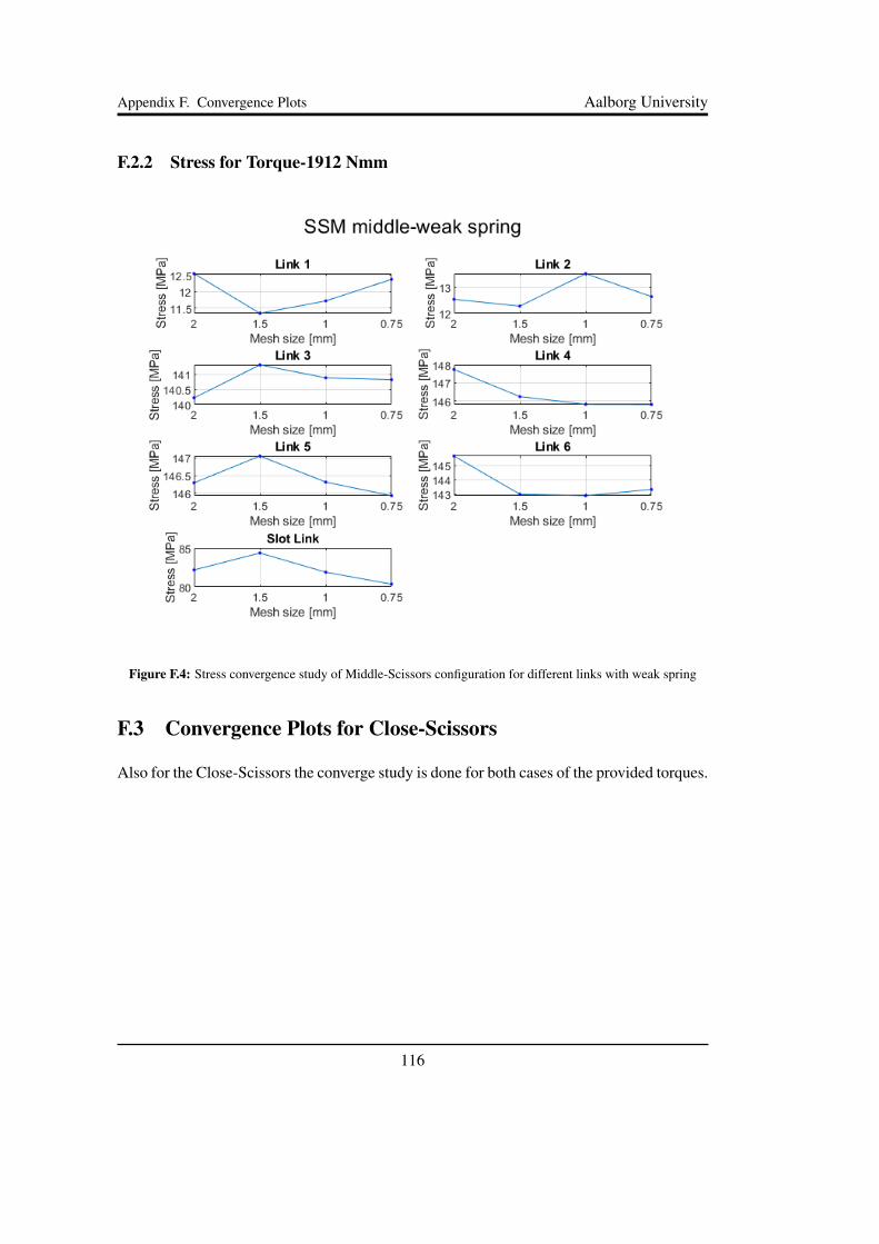
Appendix F. Convergence Plots Aalborg University
F.2.2 Stress for Torque-1912 Nmm
Figure F.4: Stress convergence study of Middle-Scissors configuration for different links with weak spring
F.3 Convergence Plots for Close-Scissors
Also for the Close-Scissors the converge study is done for both cases of the provided torques.
116
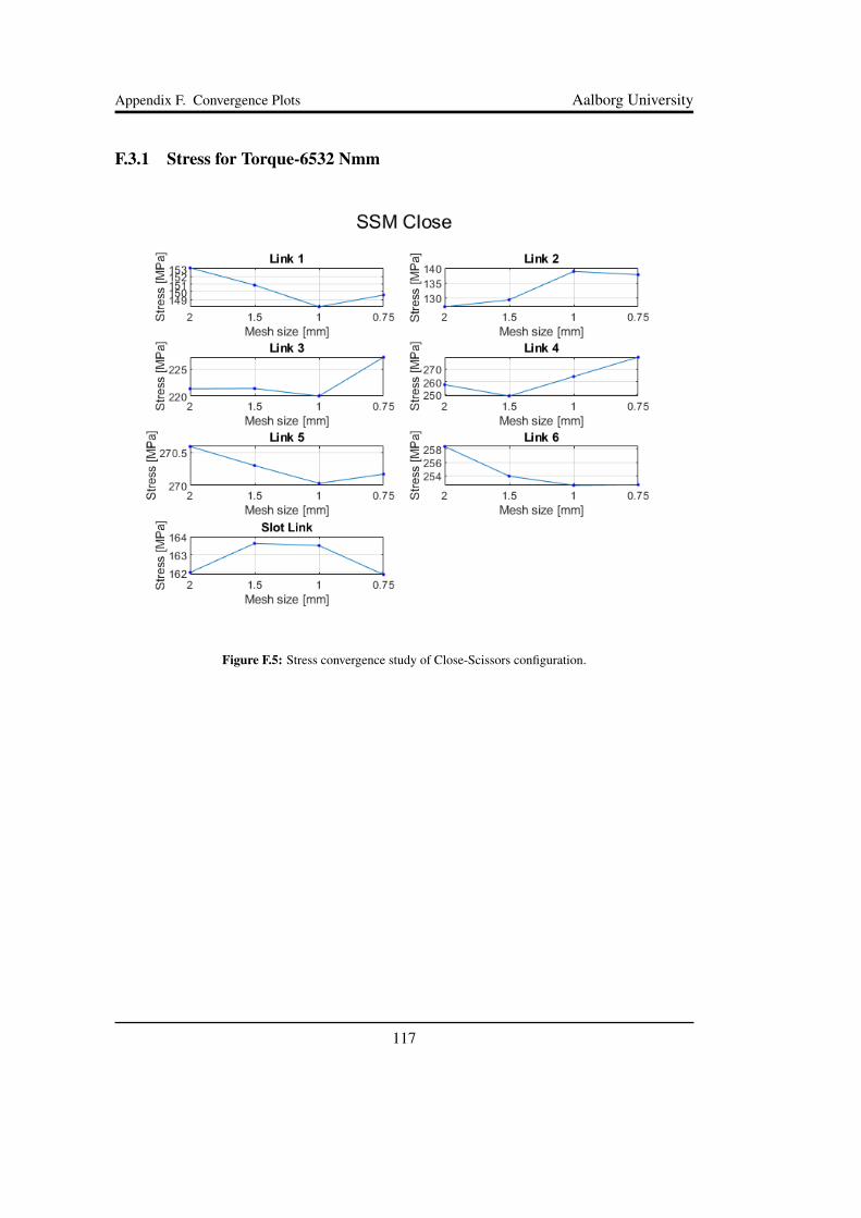
Appendix F. Convergence Plots Aalborg University
F.3.1 Stress for Torque-6532 Nmm
Figure F.5: Stress convergence study of Close-Scissors configuration.
117
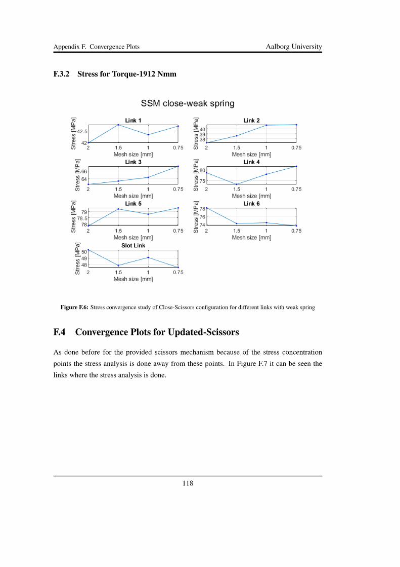
Appendix F. Convergence Plots Aalborg University
F.3.2 Stress for Torque-1912 Nmm
Figure F.6: Stress convergence study of Close-Scissors configuration for different links with weak spring
F.4 Convergence Plots for Updated-Scissors
As done before for the provided scissors mechanism because of the stress concentration
points the stress analysis is done away from these points. In Figure F.7 it can be seen the
links where the stress analysis is done.
118

Appendix F. Convergence Plots Aalborg University
Link 9
Link 7Link 5Link 4
Link 2
Link 1Link 3 Link 6 Link 8
Link 10
Figure F.7: Highlighted links where the stress analysis is done.
The convergence study for the Updated Scissors mechanism can be seen in Figure F.8.
Figure F.8: Stress convergence study of Updated-Scissors configuration for different links.
119

Appendix G
Engineering Drawings
G.1 VSM Assembly
G.1.1 VSM side
Figure G.1
120

Appendix G. Engineering Drawings Aalborg University
G.1.2 VSM Outer Disc
Figure G.2
G.1.3 VSM Inner Disc
Figure G.3
121

Appendix G. Engineering Drawings Aalborg University
G.1.4 VSM Spring Base
Figure G.4
G.1.5 VSM Cuff attachment
Figure G.5
122
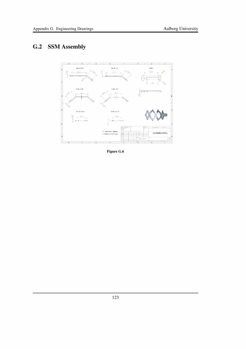
Appendix G. Engineering Drawings Aalborg University
G.2 SSM Assembly
Figure G.6
123
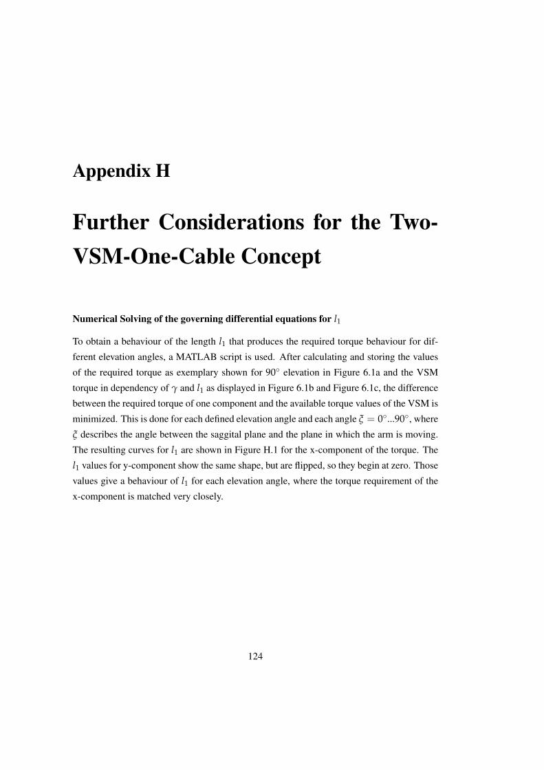
Appendix H
Further Considerations for the Two-VSM-One-Cable Concept
Numerical Solving of the governing differential equations for l1
To obtain a behaviour of the length l1 that produces the required torque behaviour for dif-
ferent elevation angles, a MATLAB script is used. After calculating and storing the values
of the required torque as exemplary shown for 90◦ elevation in Figure 6.1a and the VSM
torque in dependency of γ and l1 as displayed in Figure 6.1b and Figure 6.1c, the difference
between the required torque of one component and the available torque values of the VSM is
minimized. This is done for each defined elevation angle and each angle ξ = 0◦...90◦, where
ξ describes the angle between the saggital plane and the plane in which the arm is moving.
The resulting curves for l1 are shown in Figure H.1 for the x-component of the torque. The
l1 values for y-component show the same shape, but are flipped, so they begin at zero. Those
values give a behaviour of l1 for each elevation angle, where the torque requirement of the
x-component is matched very closely.
124
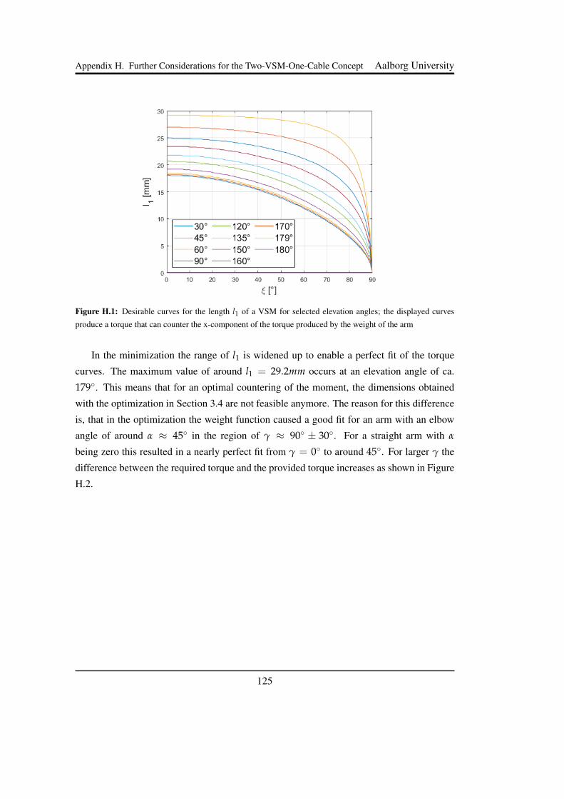
Appendix H. Further Considerations for the Two-VSM-One-Cable Concept Aalborg University
Figure H.1: Desirable curves for the length l1 of a VSM for selected elevation angles; the displayed curves
produce a torque that can counter the x-component of the torque produced by the weight of the arm
In the minimization the range of l1 is widened up to enable a perfect fit of the torque
curves. The maximum value of around l1 = 29.2mm occurs at an elevation angle of ca.
179◦. This means that for an optimal countering of the moment, the dimensions obtained
with the optimization in Section 3.4 are not feasible anymore. The reason for this difference
is, that in the optimization the weight function caused a good fit for an arm with an elbow
angle of around α ≈ 45◦ in the region of γ ≈ 90◦ ± 30◦. For a straight arm with α
being zero this resulted in a nearly perfect fit from γ = 0◦ to around 45◦. For larger γ the
difference between the required torque and the provided torque increases as shown in Figure
H.2.
125
Appendix H. Further Considerations for the Two-VSM-One-Cable Concept Aalborg University
Figure H.2: Absolute value of half the torque resulting from the weight of the arm, the torque produced by the
VSM and the difference between both for a straight arm with α = 0◦
This difference is removed by elongating l1 in the way shown in Figure H.1, because an
increasing l1 changes both, the force and the lever arm of the force.
The deviation of the VSM torque and the required shoulder torqe also differs for each
elbow angle α, thus an optimal solution for the transition is only obtained, if firstly the
length l1 has a wide range of motion and secondly if the described process of selecting the
best suiting length is gone through for each change of angle. The latter consists of relatively
simple operations and can be implemented in an controller to calculate the set point. With
that given a PID controller can be programmed to adjust l1 to the required value.
Considerations concerning the selection of the active component
For an implementation of such a mechanism with the maximum dimensions as described in
Section 3.4 the size of the mechanism becomes a problem. In an arbitrary position between
the two planes, the ideal exoskeleton still provides support for lifting the arm. As can be
seen from Figure H.1 this requires being able to shift the pulley on the inner disc to a higher
radius. As described in Reference [Bai & Li, 2019], the length of the cable and with it the
126

Appendix H. Further Considerations for the Two-VSM-One-Cable Concept Aalborg University
force acting in direction of l2 is depending on the angle of distortion θ. It is calculated by
αc = βc + γc
βc = arccos
a− 2l1 sin θ√4l2
2 − 4al1 sin θ + a2
− arccos
a√4l2
2 − 4al1 sin θ + a2
+π
2
γc = arccos
a + 2l1 sin θ√4l2
2 + 4al1 sin θ + a2
− arccos
a√4l2
2 + 4al1 sin θ + a2
+π
2
(H.1)
where a = 4Rc + 2dc. Rc is the radius that the outside of the cable is touching, dc is the
diameter of the cable. With the lengths of the free cable∣∣∣−→DB∣∣∣ = √l2
2 − al1 sin θ (H.2)∣∣∣−→EG∣∣∣ = √l2
2 + al1 sin θ (H.3)
the cable length becomes:
lc(θ) =αa2
+∣∣∣−→DB
∣∣∣+ ∣∣∣−→EG∣∣∣ (H.4)
With the cable length determined, the force acting on the pulley on the inner disc in the
direction of l2 is ∣∣∣−→Fl2
∣∣∣ = 2 (F0 + k∆lc) (H.5)
where the cable is pretensioned with F0 and the spring has a stiffness of k. ∆lc is defined as
∆lc = lc (θ)− lc (θ = 0) (H.6)
With the system described as vectors,−→l3 and
−→l1 are defined as follows, the orientation
of−→Fl2 is found.
−→l3 =
{0
l3
}(H.7)
−→l1 = |l1|
{sin θ
cos θ
}(H.8)
−→l2 =
−→l3 −
−→l1 (H.9)
−→Fl2 = |Fl2|
−−→l2∣∣∣−→l2 ∣∣∣ (H.10)
127

Appendix H. Further Considerations for the Two-VSM-One-Cable Concept Aalborg University
The force vector−→Fl1 is then found to be the projection of
−→Fl2 to the direction of
−→l1 .
−→Fl1 =
∣∣∣−→Fl2
∣∣∣ cos δ
−→l1∣∣∣−→l1 ∣∣∣ (H.11)
where delta is the angle between−→l1 and
−→l2 that is inside the triangle built from
−→l3 ,−→l1
and−→l2 .
δ = 180◦ − arccos
−→l1 ◦ −→l2∣∣∣−→l1 ∣∣∣ ∣∣∣−→l2 ∣∣∣ (H.12)
The resulting curves for the angle δ is displayed in Figure H.3.
Figure H.3: Angle included between−→l1 and
−→l2 .
With the angle found, Figure H.1 shows the magnitude of force acting on the pulley on
the inner disc for selected elevation angles. It is only the part of the force displayed that
points in the direction of−→l1 . This force will have to be overcome by a motor, if a pseudo-
active exoskeleton is built.
128

Appendix H. Further Considerations for the Two-VSM-One-Cable Concept Aalborg University
Figure H.4: Curves of Fl1 and l1 over the transition process for selected elevation angles. All numbers are
absolute numbers.
The right y-axes in Figure H.4 displays the curves for the length of l1. As is seen, the
behaviour of the force curves, that correspond to the left y-axes, is very nonlinear. The
steplike character that is shown at some areas is a result of the numerical solving of the
differential equation for l1. Based on the above estimations it can be said, that the motor has
to provide a force of greater than 464.7N as this is the maximum value obtained for l3, R, kand F0 as in Table H.1. To obtain a required power the speed needs to be known.
Variable Value
l3 31mmR 6mmk 3.1674Nmm−1
F0 4.9665N
Table H.1: Values that are used throughout the section. k and F0 are half of the values obtained in Section 3.4
to achieve 50% of support
To obtain a speed, the x-axis is transformed from the transition angle ξ to the transition
time tT, where the time to complete the transition is set to be tTmax = 1s. Then l1 is
numerically differentiated with respect to tT. To obtain values at the very end of the curve
where the highest speeds are expected, a forward differentiation is used that follows the
scheme
f ′(x) =f (x)− f (x− h)
h(H.13)
129

Appendix H. Further Considerations for the Two-VSM-One-Cable Concept Aalborg University
Figure H.5 shows the required speed of the pulley on the inner disc for selected elevation
angles. The highest values occur at the end of the range, where the change is largest. At the
begin of the transition process the required speed is fairly uniform. The highest number that
is obtained with this numerical process is 0.65ms−1.
Figure H.5: Required speed of the pulley on the inner disc for selected angles for tT = 1s
The power that is required to move the pulley to the position is the scalar product of the
force vector and the speed vector. Since both vectors already have the same orientation, the
force Fl1 is multiplied with the speed. Figure H.6 shows the resulting curves. It is seen,
that due to the numerical process the data points are very unsteady. The maximum value
obtained is about 7W.
130
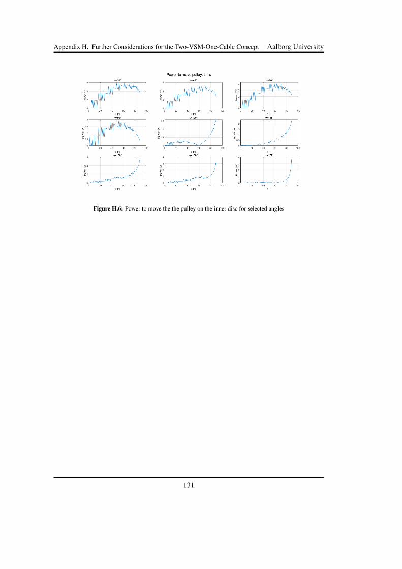
Appendix H. Further Considerations for the Two-VSM-One-Cable Concept Aalborg University
Figure H.6: Power to move the the pulley on the inner disc for selected angles
131

Appendix I
Measurements of the Range of Motion
In the following pictures of the measurements for the RoM are presented.
Figure I.1: Flexion
132
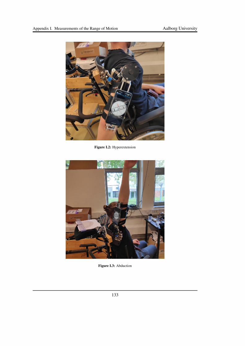
Appendix I. Measurements of the Range of Motion Aalborg University
Figure I.2: Hyperextension
Figure I.3: Abduction
133
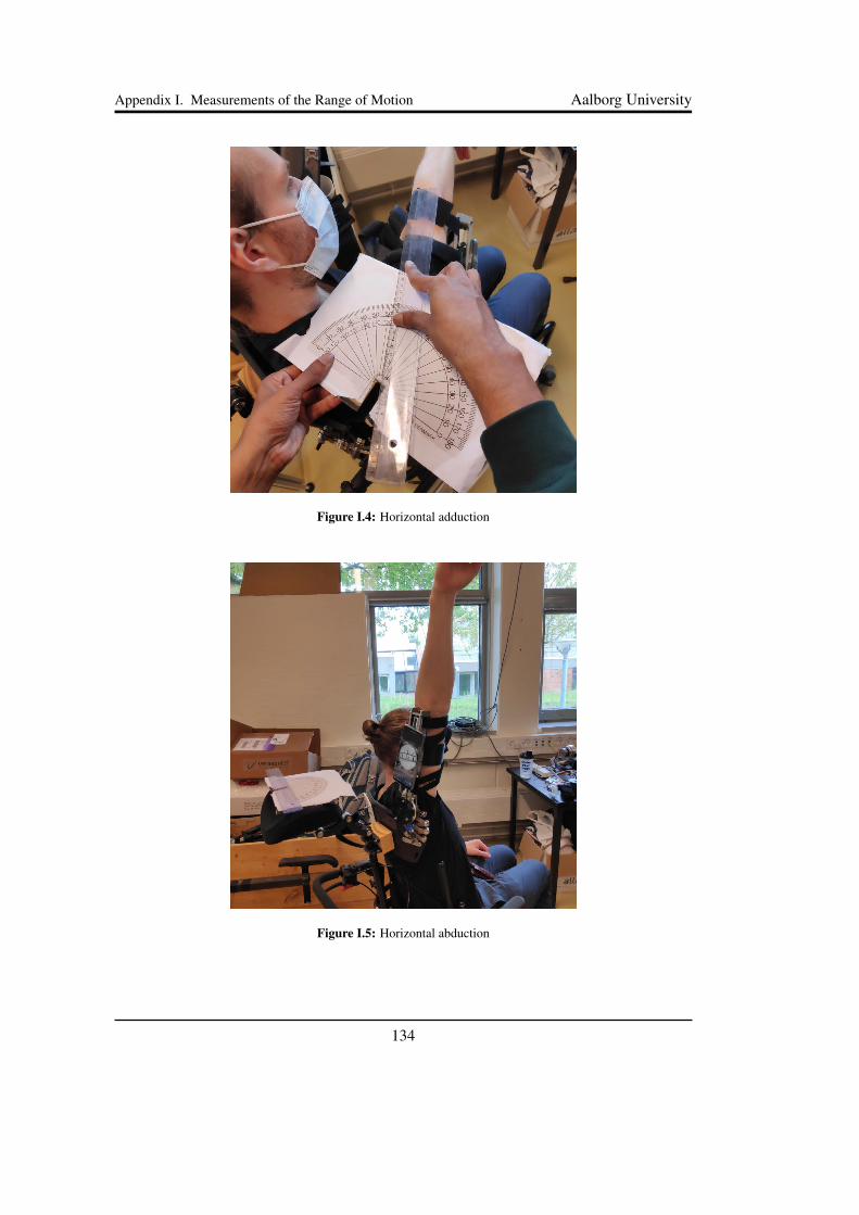
Appendix I. Measurements of the Range of Motion Aalborg University
Figure I.4: Horizontal adduction
Figure I.5: Horizontal abduction
134

Appendix J
Torque Testing with 3D Printed Pul-leys
Before the pulleys have been changed, the torque that the VSM was able to provide has been
measured. The results can be seen in Figure x. It can be seen that the friction has been larger
than the provided torque. Hence the results are not investigated further and the spring is
discarded.
Figure J.1: Results for the torque over the internal angle θ of the VSM with all measured points, the average
values for loading and unloading, the corresponding standard deviation, the analytical model and the mean of
the average values of loading and unloading
135
Appendix K
First measurement with weak spring
The conducted measurements are of two kinds. Due to the lack of an encoder, the VSM has
been pushed to a certain angle at which the value given at the reading device has been noted.
The data that is presented first was obtained by deflecting the VSM and reading the torque
after the reading stabilized. The second data was obtained by attempting to read the torque
value at the exact time the specific angle was reached. For both methods an angle increment
of 5◦ has been used and three cycles have been conducted, where one cycle consists of a full
motion to 180◦ deflection, setting the VSM to be stable and moving it back to 0◦ deflection.
The settling procedure at 180◦ deflection in the middle of a cycle consisted of reading a
torque value when coming from 175◦, adjusting the deflection angel so that the deflection
angle remains at 180◦ without outer influence and reading this new torque value before
reducing the deflection angle again. By this procedure two readings for 180◦ deflection are
obtained, the first one that belongs to the spring loading phase, and a second one that belongs
to the spring unloading phase. 37 torque values have been read per cycle per phase and are
presented in the following Figure K.1 and Figure K.2. In each figure, the measured data
points, their average and the predicted torque curve is shown. The predicted torque curve is
obtained with the Adams model described in Section x, as the numerical model is quicker to
adapt to the slightly changed pulley geometry.
136

Appendix K. First measurement with weak spring Aalborg University
(a) (b)
(c)
Figure K.1: Measured torque values after they stabilized over the shoulder angle γ for (a) the loading phase, (b)
the unloading phase and (c) both phases with the mean of both and the standard deviations of the measurements
137

Appendix K. First measurement with weak spring Aalborg University
(a) (b)
(c)
Figure K.2: Measured torque values at the time of reaching the next reading angle over the shoulder angle γ for
(a) the loading phase, (b) the unloading phase(c) both phases with the mean of both and the standard deviations
of the measurements
When observing the obtained data points closely, it is seen that the overall shapes of
the obtained curves are similar. Both kinds of reading show a clear maximum in the centre,
the data for the loading phase and the instant reading method even indicate the shift of the
maximum to small γ. When the single phases are compared to each other, it is seen that the
instant reading method gives a smaller standard deviation, but larger hysteresis.
138
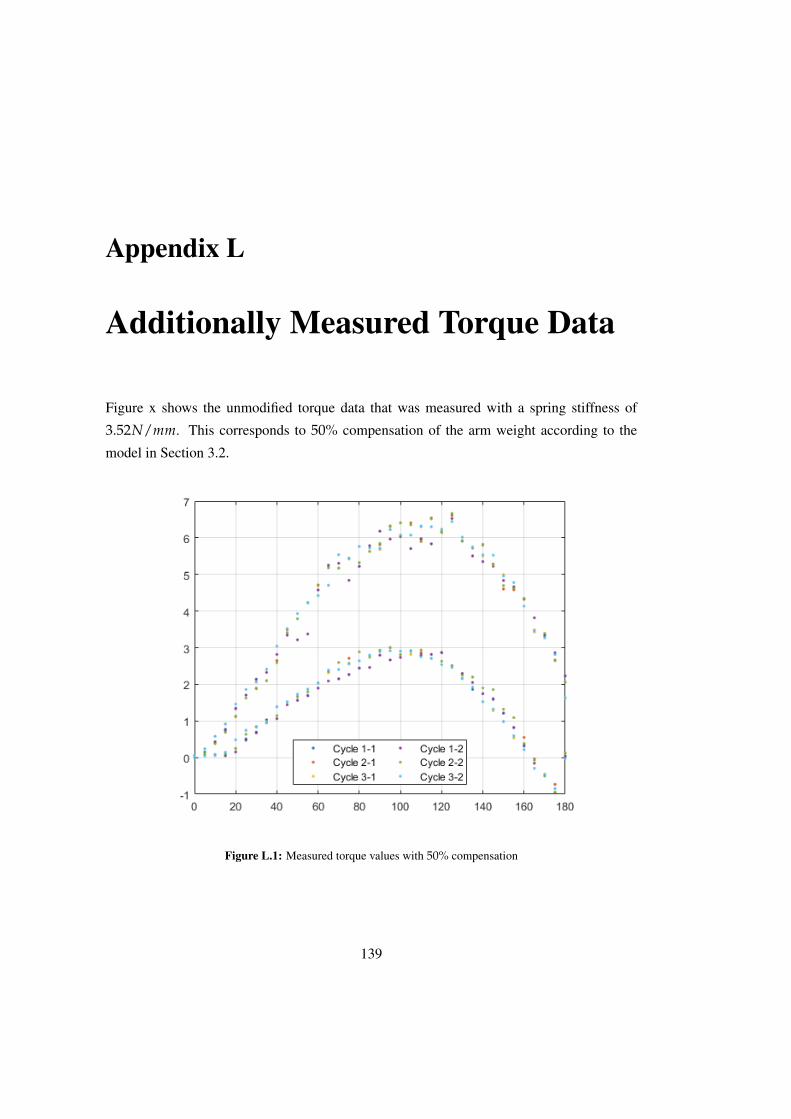
Appendix L
Additionally Measured Torque Data
Figure x shows the unmodified torque data that was measured with a spring stiffness of
3.52N/mm. This corresponds to 50% compensation of the arm weight according to the
model in Section 3.2.
Figure L.1: Measured torque values with 50% compensation
139
Related Documents