Department of Engineering Science and Mechanics … of Engineering Science and Mechanics ... f the linear viscous component ... The motion of the solid is described by the displacement

Benchmarking the Immersed Finite Element Method for

Fluid-Structure Interaction Problems

Saswati RoyDepartment of Engineering Science and Mechanics

The Pennsylvania State University212 Earth and Engineering Sciences Building

University Park PA 16802 USA

Luca Heltai∗

Scuola Internazionale Superiore di Studi AvanzatiVia Bonomea 26534136 Trieste, Italy

Francesco CostanzoCenter for Neural Engineering

The Pennsylvania State UniversityW-315 Millennium Science Complex

University Park PA 16802 USA

April 10, 2015

Abstract

We present an implementation of a fully variational formulation of an immersed methodfor fluid-structure interaction problems based on the finite element method. While typical im-plementation of immersed methods are characterized by the use of approximate Dirac deltadistributions, fully variational formulations of the method do not require the use of said distri-butions. In our implementation the immersed solid is general in the sense that it is not requiredto have the same mass density and the same viscous response as the surrounding fluid. We as-sume that the immersed solid can be either viscoelastic of differential type or hyperelastic. Herewe focus on the validation of the method via various benchmarks for fluid-structure interactionnumerical schemes. This is the first time that the interaction of purely elastic compressible solidsand an incompressible fluid is approached via an immersed method allowing a direct comparisonwith established benchmarks.

Keywords: Fluid-Structure Interaction; Fluid-Structure Interaction Benchmarking; ImmersedBoundary Methods; Immersed Finite Element Method; Finite Element Immersed Boundary Method

1 Introduction

Immersed methods for fluid structure interaction (FSI) problems were pioneered by Peskin andhis co-workers (Peskin, 1977, 2002). They proposed an approach called the immersed boundary

∗Corresponding Author. Email: Luca Heltai <[email protected]>; Tel.: +39 040 3787-449

1

arX

iv:1

306.

0936

v3 [

mat

h.N

A]

9 A

pr 2

015

method (IBM), in which the equations governing the fluid motion have body force terms describingthe FSI. The equations are integrated via a finite difference (FD) method and the body force termsare computed by modeling the solid body as a network of elastic fibers. As such, this system offorces has singular support (the boundary in the method’s name) and is implemented via Dirac-δdistributions. The configuration of the fiber network is represented via a discrete set of points whosemotion is then related to that of the fluid again via Dirac-δ distributions. We should clarify thatthe fiber network in question can be configured so as to represent both thin elastic interfaces as wellas thick elastic bodies. In the numerical implementation of this method the Dirac-δ distributionsare aproximated as functions. A recent paper by Fai et al. (2014) offers a detailed stability analysisin the context of problems with variable density and viscosity.

Immersed methods based on the finite element method (FEM) has been formulated by variousauthors (Boffi and Gastaldi, 2003; Boffi et al., 2008; Wang and Liu, 2004; Zhang et al., 2004a).Boffi and Gastaldi (2003) were the first to show that a variational approach to immersed methodsdoes not necessitate the approximation of Dirac-δ distributions as they naturally disappears inthe weak formulation. The thrust of the work by Wang and Liu (2004) and Zhang et al. (2004a)was to remove the requirement that the immersed solid be a fiber network. They also included theability to accommodate density differences between solid and fluid, as well as compressible materialsin addition to incompressible ones. While they proposed an approach applicable to solid bodiesof general topological and constitutive characteristics they maintained the use of approximatedDirac-δ distribution through a strategy called the reproducing kernel particle method (RKPM).

Recently, Heltai and Costanzo (2012) proposed a generalization of the approach by Boffi et al.(2008) in which a fully variational FEM formulation is shown to be applicable to problems withimmersed bodies of general topological and constitutive characteristics and without the use of Dirac-δ distributions. The discussion in Heltai and Costanzo (2012) focused on the construction of naturalinterpolation operators between the fluid and the solid discrete spaces that guarantee semi-discretestability estimates and strong consistency. Since the formulation in Heltai and Costanzo (2012) isapplicable to solid bodies with pure hyperelastic behavior, i.e., without a viscous component in thestress response, in this paper we show that the method in question satisfies the benchmark tests byTurek and Hron (2006). This is an important result given that these benchmarks have become a defacto standard in the FSI computational community, and given that previous immersed methodscould not satisfy them due to intrinsic model restrictions. In this sense, and to the best of ourknowledge, our results are the first of their kind. Along with these important results, we alsoillustrate the application of our method to a three-dimensional problem whose geometry is similarto that in the two-dimensional benchmark tests.

2 Formulation

2.1 Basic notation and governing equations

Referring to Fig. 1, Bt is a body immersed in a fluid, the latter occupying Ω \ Bt, where Ω is afixed control volume. The body’s motion is described by a diffeomorphism ζ : B → Bt, x = ζ(s, t),where B is the body’s reference configuration, s ∈ B, x ∈ Ω, and time t ∈ [0, T ), with T > 0.Away from boundaries, the motion Bt and the fluid are both governed by the balance of mass andmomentum, respectively,

∂ρ

∂t+∇ · (ρu) = 0 and ∇ · σ + ρb = ρ

[∂u

∂t+ (∇u)u

], (1)

2

Figure 1: Current configuration Bt of a body B immersed in a fluid occupying the domain Ω.

where ρ(x, t) is the mass density, u(x, t) is the velocity, σ(x, t) is the Cauchy stress, b(x, t) is theexternal force density per unit mass, and where ∇ and (∇ · ) denote the gradient and divergenceoperators, respectively. Equations (1) hold both for the solid and the fluid, which can be distin-guished via their constitutive equations. We assume that u(x, t) is continuous across ∂Bt, theboundary of Bt. Along with the jump conditions for the momentum balance laws, this implies thatthe traction field is also continuous across ∂Bt. Equations (1) are complemented by the followingboundary conditions:

u(x, t) = ug(x, t), for x ∈ ∂ΩD, and σ(x, t)n(x, t) = sg(x, t), for x ∈ ∂ΩN , (2)

where ug and sg are prescribed velocity and surface traction fields, n is the outward unit normalto ∂Ω, and where ∂ΩD ∪ ∂ΩN = ∂Ω and ∂ΩD ∩ ∂ΩN = ∅.

Fluid’s constitutive response. The fluid is assumed to be Newtonian with constant massdensity ρf and stress

σ = −pI + σvf and σvf = µf

(∇u+∇uT

), (3)

where f stands for ‘fluid,’ p is the pressure, I is the identity tensor, σvf the linear viscous componentof the stress, and µf > 0 is the dynamic viscosity. For constant ρf , the first of Eqs. (1) reduces to∇ · u = 0 (x ∈ Ω \Bt) and p is a multiplier for the enforcement of this constraint.

Solid’s constitutive response. We consider both incompressible and compressible materials.For the incompressible case, Cauchy stress is assumed to be

σ = −pI + σes + σvs , (4)

where s stands for ‘solid,’ p is a multiplier enforcing incompressibility, and where σes and σvs arethe elastic and viscous parts of the stress, respectively:

σes = J−1PesFT, Pes =

∂W es (F)

∂F, and σvs = µs

(∇u+∇uT

), (5)

where W es is the elastic strain energy per unit referential volume, F = ∂ζ(s, t)/∂s is the deformation

gradient, J = detF, Pes is the first Piola-Kirchhoff stress tensor, and µs is the solid’s dynamicviscosity. The constitutive response for the compressible case is identical to that in Eq. (4) exceptfor the multiplier p, which is not needed in this case. Whether compressible or incompressible, weassume that µs ≥ 0, that is, we assume that µs might be equal to zero, in which case the solid is

3

purely elastic. We assume that W es (F) is a C1 convex function over the set of second order tensor

with positive determinant. Finally, ρs0(s) is the referential solid’s mass density and we recall thatthe first of Eq. (1) is equivalently expressed as ρs0(s) = ρs(x, t)

∣∣x=ζ(s,t)

J(s, t) (s ∈ B).

3 Variational and Discrete Formulations

The results in this paper have been obtained using the method in Heltai and Costanzo (2012). Forthe sake of completeness, here we summarize the essential elements of this method.

Our formulation has a single velocity field representing the velocity of the fluid for x ∈ Ω \ Btand the velocity of the solid for x ∈ Bt. The motion of the solid is described by the displacementfield w(s, t) := ζ(s, t)− s (s ∈ B), which is therefore related to the velocity as follows:

w(s, t) = u(x, t)∣∣x=ζ(s,t)

. (6)

The practical enforcement of Eq. (6) is crucial to distinguish an immersed method from another.In the original IBM, Eq. (6) was enforced via Dirac-δ distributions. In the present formulation,we enforce Eq. (6) variationally. Our approach can be seen as a special case of what is discussedin Boffi et al. (2014), where Eq. (6) is enforced through a Lagrange multiplier.

3.1 Functional setting

The principal unknowns of our fluid-structure interaction problem are the fields

u(x, t), p(x, t), and w(s, t), with x ∈ Ω, s ∈ B, and t ∈ [0, T ). (7)

The functional spaces for these fields are

u ∈ V = H1D(Ω)d :=

u ∈ L2(Ω)d

∣∣∇xu ∈ L2(Ω)d×d,u|∂ΩD= ug

, (8)

p ∈ Q := L2(Ω), (9)

w ∈ Y = H1(B)d :=w ∈ L2(B)d

∣∣∇sw ∈ L2(B)d×d, (10)

where ∇x and ∇s denote the gradient operators relative to x and s, respectively.For convenience, we will use a prime to denote partial differentiation with respect to time:

u′(x, t) :=∂u(x, t)

∂tand w′(s, t) :=

∂w(s, t)

∂t. (11)

Equations (8) and (9) imply that the fields u and p are defined everywhere in Ω. Because u isdefined everywhere in Ω, the function σvf is defined everywhere in Ω as well. For consistency, wemust also extend the domain of definition of the mass density of the fluid. Hence, we formallyassume that

ρf ∈ L∞(Ω). (12)

Referring to Eq. (8), the function space for the velocity test functions is V0, defined as

V0 = H10 (Ω)d :=

v ∈ L2(Ω)d

∣∣∇xv ∈ L2(Ω)d×d,v|∂ΩD= 0

. (13)

4

3.2 Governing equations: incompressible solid

When the solid is incompressible, the mass densities the fluid and the solid are constant, and thegoverning equations can be given the following form (Heltai and Costanzo, 2012):∫

Ωρf

[u′ + (∇xu)u− b

]· vv. −

∫Ωp(∇x · v)v. +

∫Ωσvf · ∇xvv. −

∫∂ΩN

sg · va.

+

∫B

[ρs0(s)− ρfJ(s, t)]

u′(x, t) +

[∇xu(x, t)

]u(x, t)− b(x, t)

· v(x)

∣∣x=ζ(s,t)

V.

+

∫BJ(s, t)

(σvs − σvf

)· ∇xv(x)

∣∣x=ζ(s,t)

V.

+

∫BPes F

T(s, t) · ∇xv(x)∣∣x=ζ(s,t)

V. = 0 ∀v ∈ V0, (14)∫Ωq(∇ · u)v. = 0 ∀q ∈ Q, (15)

ΦB

∫B

[w′(s, t)− u(x, t)

∣∣x=ζ(s,t)

]· y(s)V. = 0 ∀y ∈ Y , (16)

where ΦB is a constant with dimensions of mass over time divided by length cubed, i.e., dimensionssuch that, in 3D, the volume integral of the quantity ΦBw

′ has the same dimensions as a force.Equation (14) is obtained from the second of Eqs. (1) in a conventional way, i.e., by first

constructing the scalar product with a test function v ∈ V0, then integrating over Ω, and finallyapplying the divergence theorem. As the equation in question is supported over the entire domainΩ, we proceed to treat integrals over Ω in the following manner. Let φ represent a generic quantitywith expressions φf and φs over the fluid and solid domains, respectively. Also, let φf represent theextension of φf over Ω (see Eq. (12) and discussion proceeding it). Then, we have∫

Ωφv. =

∫Ω\Bt

φf +

∫Bt

φsv.

=

∫Ωφfv. +

∫Bt

(φs − φf)v.

=

∫Ωφfv. +

∫B

[(φs − φf ) ζ]JV. , (17)

where the last term in the above expression is simply the evaluation of the integral over Bt as anintegral over the reference configuration B.

Equation (15) is obtained from the first of Eq. (1) by constructing the scalar product withtest functions in Q (see Eq. (9)) and then integrating over Ω. Finally, Eq. (16) is obtained byconstructing the scalar product of Eq. (6) with test functions in Y (see Eq. (10)) and integratingover B.

We note that a key element of any fully variational formulation of immersed methods is (thevariational formulation of) the equation enabling the tracking of the motion of the solid, hereEq. (16). In the discrete formulation, this relation is as general as the choice of the finite-dimensionalfunctional subspaces approximating V and Y and it is key to the stability of the method. We notethat a new approach for the solid motion equation has recently been presented by Boffi et al.(2014) employing distributed Lagrange multipliers. As it turns out, this formulation, which canhandle problems with variable density and viscosity, yields unconditionally stable semi-implicittime advancing scheme.

5

3.3 Governing equations: compressible solid

When the solid is compressible, the contribution of p to the balance of linear momentum and theincompressibility constraint must be restricted to the domain Ω \Bt. Therefore, the weak problemis rewritten as follows:∫

Ωρf(u− b) · vv. −

∫Ωp∇ · vv. +

∫Ωσvf · ∇xvv. −

∫∂ΩN

sg · va.

+

∫B

[ρs0(s)− ρf0 ][u(x, t)− b(x, t)] · v(x)

∣∣x=ζ(s,t)

V.

+

∫BJ(s, t)p(x, t)∇ · v(x)

∣∣x=ζ(s,t)

V.

+

∫BJ(s, t)

(σvs − σvf

)· ∇xv(x)

∣∣x=ζ(s,t)

V.

+

∫BPes F

T(s, t) · ∇xv(x)∣∣x=ζ(s,t)

V. = 0 ∀v ∈ V0. (18)∫Ωq∇ · uv. −

∫Bt

q∇ · uv. = 0, (19)

ΦB

∫B

[w(s, t)− u(x, t)

∣∣x=ζ(s,t)

]· y(s)V. = 0 ∀y ∈ Y . (20)

Equations (18)–(20) would allow us to determine a unique solution if the field p were restricted tothe domain Ω\Bt. However, our numerical scheme requires the domain of p to be Ω. To sufficientlyconstraint the behavior of p over Bt, we have considered two possible strategies. One is to set tozero the restriction of p to Bt. The other is physically motivated and based on the fact that, for aNewtonian fluid, p is the mean normal stress. Hence, p can be constrained on Bt so to represent themean normal stress everywhere in Ω. Given the constitutive response function of a compressiblesolid material, the corresponding mean normal stress is

ps[u,w] = − 1

tr I

[σvs [u] · I + J−1[w]Pes [w] · F[w]

]. (21)

With this in mind, we replace Eq. (19) with the following equation:

−∫

Ωq∇ · uv. +

∫BJ(s, t)q(x)∇ · u(x, t)

∣∣x=ζ(s,t)

V.

+

∫Bc1J(s, t)

[p(x, t)− c2ps[u,w]

]q(x)

∣∣x=ζ(s,t)

V. = 0 ∀q ∈ Q, (22)

where c1 > 0 is a constant parameter with dimensions of length times mass over time, and wherec2 is a dimensionless constant with values 0 or 1. For c2 = 0, p = 0 (weakly) over Bt, whereas forc2 = 1, p is (weakly) constrained to be the mean normal stress everywhere in Ω.

Equations presented above can be compactly reformulated in terms of the Hilbert space Z :=V ×Q × Y , and Z0 := V0 ×Q × Y with inner product given by the sum of the inner productsof the generating spaces. Defining Z 3 ξ := [u, p,w]T and Z0 3 ψ := [v, q,y]T, we can given ourproblem the following form:

Problem 1 (Grouped dual formulation). Given an initial condition ξ0 ∈ Z , for all t ∈ (0, T ) findξ(t) ∈ Z , such that

〈F(t, ξ, ξ′), ψ〉 = 0, ∀ψ ∈ Z0, (23)

6

where F : Z 7→ Z ∗0 , Z ∗

0 is the dual of Z0, and the precise definition of the operator F can bededuced from the integral expressions in Eqs. (14)–(16) for the incompressible case and Eqs. (18),(20), and (22) for the compressible case (see Heltai and Costanzo, 2012 for additional details).

Remark 1 (Initial condition for the pressure). In Problem 1, an initial condition for the tripleξ0 = [u0, p0,w0]T is required just as a matter of compact representation of the problem. However,only the initial conditions u0 and w0 are used, since there is no time derivative acting on p.

Remark 2 (Energy estimates). Heltai and Costanzo (2012) have shown that the formulation pre-sented thus far leads to energy estimates that that are formally identical to those of the continuousformulation.

3.4 Spatial Discretization by finite elements

Domains Ω and B are decomposed into independent triangulations Ωh and Bh, respectively, con-sisting of cells K (triangles or quadrilaterals in 2D, and tetrahedra or hexahedra in 3D) such that

1. Ω = ∪K ∈ Ωh, and B = ∪K ∈ Bh;

2. Any two cells K,K ′ only intersect in common faces, edges, or vertices;

3. The decomposition Ωh matches the decomposition ∂Ω = ∂ΩD ∪ ∂ΩN .

On Ωh and Bh, finite dimensional subspaces Vh ⊂ V , Qh ⊂ Q, and Yh ⊂ Y are defined such that

Vh :=uh ∈ V

∣∣uh|K ∈ PV (K), K ∈ Ωh

≡ spanvih

NVi=1, (24)

Qh :=ph ∈ Q

∣∣ ph|K ∈ PQ(K), K ∈ Ωh

≡ spanqih

NQ

i=1, (25)

Yh :=wh ∈ Y

∣∣wh|K ∈ PY (K), K ∈ Bh≡ spanyih

NYi=1, (26)

where PV (K), PQ(K) and PY (K) are polynomial spaces of degree rV , rQ and rY respectively onthe cells K, and NV , NQ and NY are the dimensions of each finite dimensional space. Notice thatwe use only one discrete space for both u and u′ and one for w and w′, even though the continuousfunctional spaces should be different, as discussed in details in Heltai and Costanzo (2012). Also,we chose the pair Vh and Qh so as to satisfy the inf-sup condition for existence, uniqueness, andstability of solutions of the Navier-Stokes component of the problem (see, e.g., Brezzi and Fortin,1991).

3.5 Variational velocity coupling

The implementation of operator with support over Ω is common in FEM approaches to the Navier-Stokes equation. What is less common in the practical implementation of operators defined overBh involving the evaluation of fields supported over Ωh. Here we outline the basic features ofthe implementation (see also Heltai and Costanzo, 2012). As a specific example, we describe thetreatment of the operator coupling the velocities of the fluid and of the solid domain. Referringto the terms involving ΦBu(x, t)

∣∣x=ζ(s,t)

· y(s) in Eqs. (16) and (20), we define a matrix Mwu(w)

whose ij element is given by

M ijwu(wh) = ΦB

∫Bvjh(x)

∣∣x=s+wh(s,t)

· yih(s)V. . (27)

7

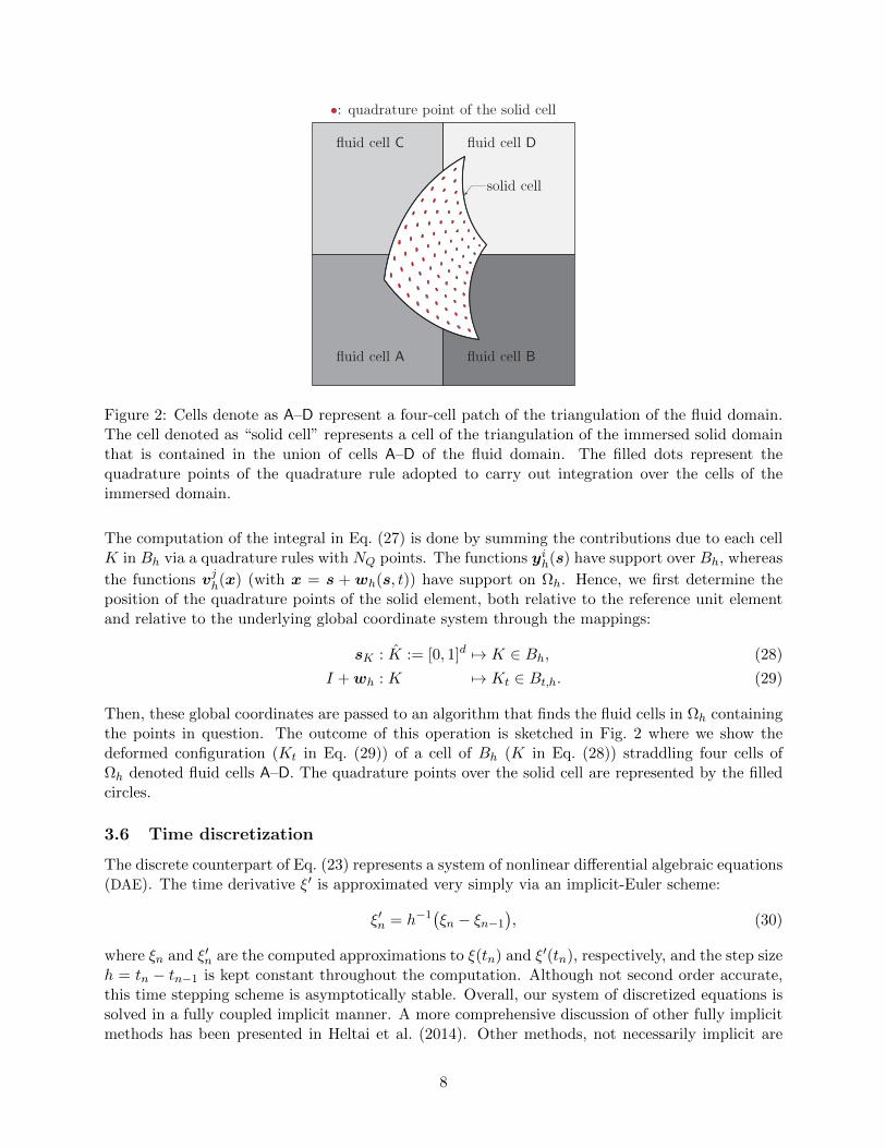
Figure 2: Cells denote as A–D represent a four-cell patch of the triangulation of the fluid domain.The cell denoted as “solid cell” represents a cell of the triangulation of the immersed solid domainthat is contained in the union of cells A–D of the fluid domain. The filled dots represent thequadrature points of the quadrature rule adopted to carry out integration over the cells of theimmersed domain.

The computation of the integral in Eq. (27) is done by summing the contributions due to each cellK in Bh via a quadrature rules with NQ points. The functions yih(s) have support over Bh, whereas

the functions vjh(x) (with x = s + wh(s, t)) have support on Ωh. Hence, we first determine theposition of the quadrature points of the solid element, both relative to the reference unit elementand relative to the underlying global coordinate system through the mappings:

sK : K := [0, 1]d 7→ K ∈ Bh, (28)

I +wh : K 7→ Kt ∈ Bt,h. (29)

Then, these global coordinates are passed to an algorithm that finds the fluid cells in Ωh containingthe points in question. The outcome of this operation is sketched in Fig. 2 where we show thedeformed configuration (Kt in Eq. (29)) of a cell of Bh (K in Eq. (28)) straddling four cells ofΩh denoted fluid cells A–D. The quadrature points over the solid cell are represented by the filledcircles.

3.6 Time discretization

The discrete counterpart of Eq. (23) represents a system of nonlinear differential algebraic equations(DAE). The time derivative ξ′ is approximated very simply via an implicit-Euler scheme:

ξ′n = h−1(ξn − ξn−1

), (30)

where ξn and ξ′n are the computed approximations to ξ(tn) and ξ′(tn), respectively, and the step sizeh = tn − tn−1 is kept constant throughout the computation. Although not second order accurate,this time stepping scheme is asymptotically stable. Overall, our system of discretized equations issolved in a fully coupled implicit manner. A more comprehensive discussion of other fully implicitmethods has been presented in Heltai et al. (2014). Other methods, not necessarily implicit are

8

possible but have not been explored yet, at least by the authors. As noted earlier, Boffi et al. (2014)have recently presented a variational formulation using distributed Lagrange multipliers, with aninteresting unconditionally stable time advancing scheme.

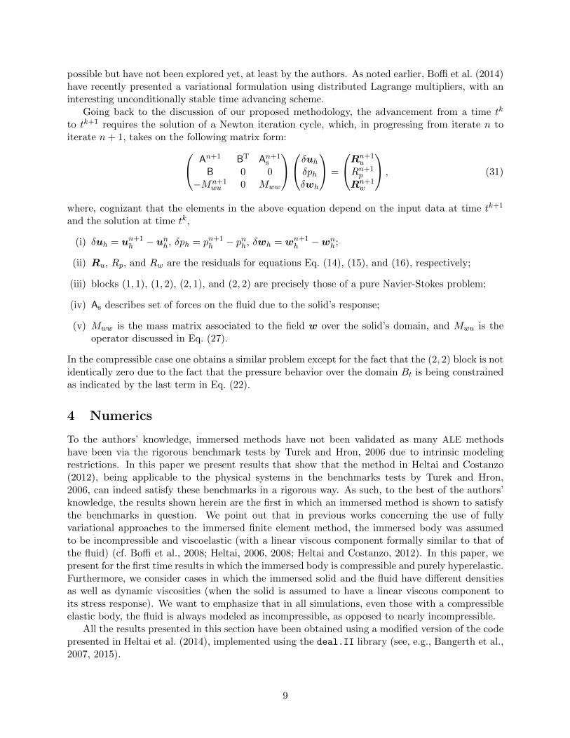
Going back to the discussion of our proposed methodology, the advancement from a time tk

to tk+1 requires the solution of a Newton iteration cycle, which, in progressing from iterate n toiterate n+ 1, takes on the following matrix form: An+1 BT An+1

s

B 0 0−Mn+1

wu 0 Mww

δuhδphδwh

=

Rn+1u

Rn+1p

Rn+1w

, (31)

where, cognizant that the elements in the above equation depend on the input data at time tk+1

and the solution at time tk,

(i) δuh = un+1h − unh, δph = pn+1

h − pnh, δwh = wn+1h −wn

h;

(ii) Ru, Rp, and Rw are the residuals for equations Eq. (14), (15), and (16), respectively;

(iii) blocks (1, 1), (1, 2), (2, 1), and (2, 2) are precisely those of a pure Navier-Stokes problem;

(iv) As describes set of forces on the fluid due to the solid’s response;

(v) Mww is the mass matrix associated to the field w over the solid’s domain, and Mwu is theoperator discussed in Eq. (27).

In the compressible case one obtains a similar problem except for the fact that the (2, 2) block is notidentically zero due to the fact that the pressure behavior over the domain Bt is being constrainedas indicated by the last term in Eq. (22).

4 Numerics

To the authors’ knowledge, immersed methods have not been validated as many ALE methodshave been via the rigorous benchmark tests by Turek and Hron, 2006 due to intrinsic modelingrestrictions. In this paper we present results that show that the method in Heltai and Costanzo(2012), being applicable to the physical systems in the benchmarks tests by Turek and Hron,2006, can indeed satisfy these benchmarks in a rigorous way. As such, to the best of the authors’knowledge, the results shown herein are the first in which an immersed method is shown to satisfythe benchmarks in question. We point out that in previous works concerning the use of fullyvariational approaches to the immersed finite element method, the immersed body was assumedto be incompressible and viscoelastic (with a linear viscous component formally similar to that ofthe fluid) (cf. Boffi et al., 2008; Heltai, 2006, 2008; Heltai and Costanzo, 2012). In this paper, wepresent for the first time results in which the immersed body is compressible and purely hyperelastic.Furthermore, we consider cases in which the immersed solid and the fluid have different densitiesas well as dynamic viscosities (when the solid is assumed to have a linear viscous component toits stress response). We want to emphasize that in all simulations, even those with a compressibleelastic body, the fluid is always modeled as incompressible, as opposed to nearly incompressible.

All the results presented in this section have been obtained using a modified version of the codepresented in Heltai et al. (2014), implemented using the deal.II library (see, e.g., Bangerth et al.,2007, 2015).

9

4.1 Discretization

The approximation spaces we used in our simulations for the approximations of the velocity fielduh and of the displacement field wh are the piecewise bi-quadratic spaces of continuous vectorfunctions over Ω and over B, respectively, which we will denote by Q2

0 space.∗ For the pressurefield p, in some cases we have used the piecewise continuous bi-linear space Q1

0 and in other casesthe piecewise discontinuous linear space P1

−1 over Ω. Both the Q20-|Q1

0 and the Q20|P1−1 pairs of

spaces are known to satisfy the inf-sup condition for the approximation of the Navier-Stokes part ofour equations (see, e.g., Brezzi and Fortin, 1991). The choice of the space Q2

0 for the displacementvariable wh is a natural choice, given the underlying velocity field uh. With this choice of spaces,Eqs. (16) and (20) can be satisfied exactly when the solid and the fluid meshes are matching.

4.2 Results for Incompressible Immersed Solids

4.2.1 Static equilibrium of an annular solid comprising circumferential fibers andimmersed in a stationary fluid

This numerical test is motivated by the ones presented in Boffi et al. (2008); Griffith and Luo (2012)and it pertains to the case of an incompressible solid with both elastic and viscous components ofthe stress response. The objective of this test is to compute the equilibrium state of an initiallyundeformed thick annular cylinder submerged in a stationary incompressible fluid that is containedin a rigid prismatic box having a square cross-section.

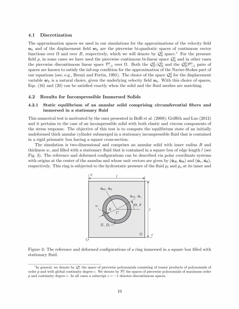
The simulation is two-dimensional and comprises an annular solid with inner radius R andthickness w, and filled with a stationary fluid that is contained in a square box of edge length l (seeFig. 3). The reference and deformed configurations can be described via polar coordinate systemswith origins at the center of the annulus and whose unit vectors are given by (uR, uΘ) and (ur, uθ),respectively. This ring is subjected to the hydrostatic pressure of the fluid pi and po at its inner and

Figure 3: The reference and deformed configurations of a ring immersed in a square box filled withstationary fluid.

∗In general, we denote by Qpc the space of piecewise polynomials consisting of tensor products of polynomials of

order p and with global continuity degree c. We denote by Ppc the spaces of piecewise polynomials of maximum order

p and continuity degree c. In all cases a subscript c = −1 denotes discontinuous spaces.

10

outer walls, respectively. Negligible body forces act on the system and there is no inflow or outflowof fluid across the walls of the box. Since both the solid and the fluid are incompressible, neitherthe annulus nor the fluid will move and the problem reduces to determining the Lagrange multiplierfield p. The elastic behavior of the ring is governed by a continuous distribution of concentric fiberslying in the circumferential direction. The first Piola-Kirchhoff and the Cauchy stress tensors arethen given by, respectively,

P = −psF−T +GeFuΘ ⊗ uΘ and σs = −psI +Geuθ ⊗ uθ, (32)

where Ge is a constant modulus of elasticity, ps is the Lagrange multiplier that enforces incom-pressibility of the ring and uθ = uΘ (since deformed and reference configurations coincide). Recallthat in the proposed immersed FEM we have a single field p representing the Lagrange multipliereverywhere, whether in the fluid or in the solid. Therefore, we have p = ps in the solid. With thisin mind, we observe that the equilibrium stress state in the fluid is purely hydrostatic. Further-more, since the boundary conditions on ∂Ω is of homogeneous Dirichlet type, the solution for theLagrange multiplier p over Ω is not unique. We remove the non uniqueness by enforcing a zeroaverage constraint on the field p. Then it can be shown (cf. Heltai et al., 2014) that the solutionfor the field p is as follows:

p =

po = −πGe

2l2

((R+ w)2 −R2

)for R+ w ≤ r,

ps = Ge ln(R+wr )− πGe

2l2

((R+ w)2 −R2

)for R < r < R+ w,

pi = Ge ln(1 + wR)− πGe

2l2

((R+ w)2 −R2

)for r ≤ R,

(33)

with velocity of fluid u = 0 and the displacement of the solid w = 0. Note that Eq. (33) is differentfrom Eq. (69) of Boffi et al. (2008), where p varies linearly with r (we believe this to be in error).

For all our numerical simulations we have used R = 0.25 m, w = 0.062,50 m, l = 1.0 m andGe = 1 Pa and for these values we obtain pi = 0.167,92 Pa and po = −0.055,22 Pa using Eq. (33).We have used ρ = 1.0 kg/m3, dynamic viscosities µf = µs = µ = 1.0 Pa·s, and time step sizeh = 1× 10−3 s in our tests. For all our numerical tests we have used Q2

0 elements to represent w ofthe solid, whereas we have used (i) Q2

0|P1−1 elements, and (ii) Q2

0|Q10 elements to represent v and

p over the control volume. We present a sample profile of p over the entire control volume and itsvariation along different values of y, after one time step, in Fig. 4 and Fig. 5 for Q2

0|P1−1 and Q2

0|Q10

elements, respectively.The convergence rate (see, Tables 1 and 2 for Q2

0|P1−1 and Q2

0|Q10 elements, respectively) is 2.5

for the L2 norm of the velocity, 1.5 for the H1 norm of the velocity and 1.5 for the L2 norm of thepressure which matches the rates presented in Boffi et al. (2008). In all these numerical tests wehave used 1,856 cells with 15,776 DoFs for the solid.

4.2.2 Disk entrained in a lid-driven cavity flow

We test the volume conservation of our numerical method by measuring the change in the area ofa disk that is entrained in a lid-driven cavity flow of an incompressible, linearly viscous fluid. Thisis another example pertaining to a system with an incompressible solid with stress response thatincludes both elastic and viscous contributions. This test is motivated by similar ones presentedin Griffith and Luo (2012); Wang and Zhang (2010). Referring to Fig. 6, the disk has a radius

11

(a) Over the entire domain

x (m)

Pressure

(Pa)

0 0.2 0.4 0.6 0.8 1

−0.05

0

0.05

0.1

0.15

0.2 0.2 m 0.3 m 0.4 m 0.5 m

(b) At different values of y

Figure 4: The values of p after one time step when using P1−1 elements for p.

Table 1: Error convergence rate obtained when using P1−1 element for p after one time step.

No. of cells No. of DoFs ‖uh − u‖0 ‖uh − u‖1 ‖ph − p‖0256 2,946 2.00605e-05 - 1.95854e-03 - 6.71603e-03 -

1,024 11,522 3.69389e-06 2.44 7.44696e-04 1.40 2.47476e-03 1.444,096 45,570 5.76710e-07 2.68 2.25134e-04 1.73 8.74728e-04 1.5016,384 181,250 1.06127e-07 2.44 8.24609e-05 1.45 3.14028e-04 1.48

(a) Over the entire domain

x (m)

Pressure

(Pa)

0 0.2 0.4 0.6 0.8 1

−0.05

0

0.05

0.1

0.15

0.2 0.2 m 0.3 m 0.4 m 0.5 m

(b) At different values of y

Figure 5: The values of p after one time step when using Q10 elements for p.

12

Table 2: Error convergence rate obtained when using Q10 element for p after one time step.

No. of cells No. of DoFs ‖uh − u‖0 ‖uh − u‖1 ‖ph − p‖0256 2,467 4.36912e-05 - 2.79237e-03 - 7.39310e-03 -

1,024 9,539 6.14959e-06 2.83 9.02397e-04 1.63 2.42394e-03 1.614,096 37,507 1.28224e-06 2.26 3.49329e-04 1.37 9.10608e-04 1.4116,384 148,739 2.33819e-07 2.46 1.25626e-04 1.48 3.27256e-04 1.48

R = 0.2 m and its center C is initially positioned at x = 0.6 m and y = 0.5 m in the squarecavity whose each edge has the length l = 1.0 m. Body forces on the system are negligible. Theconstitutive elastic response of the disk is as follows:

P = −psI +GeF. (34)

We have used the following parameters: ρ = 1.0 kg/m3, dynamic viscosities µf = µs = µ =0.01 Pa·s, elastic shear modulus Ge = 0.1 Pa and U = 1.0 m/s. For our numerical simulations wehave used Q2

0 elements to represent w of the disk whereas we have used Q20|P1−1 element for the

fluid. The disk is represented using 320 cells with 2,626 DoFs and the control volume has 4,096 cellsand 45,570 DoFs. The time step size h = 1 × 10−2 s. We consider the time interval 0 < t ≤ 8 sduring which the disk is lifted from its initial position along the left vertical wall, drawn alongunderneath the lid and finally dragged downwards along the right vertical wall of the cavity (seeFig. 7). As the disk trails beneath the lid, it experiences large shearing deformations (see Fig. 8).Due to incompressibility, the disk should have retained its original area over the course of time.However, as shown in Fig. 9(a), from our numerical scheme we obtain an area change of the diskof about 4%. As discussed in great detail by Griffith (2012), immersed methods are prone to poorvolume conservation and a number of approaches have been proposed in the literature to addressthis issue. The error shown in Fig. 9(a) is more than that in Griffith and Luo (2012) which is onlyof about 0.5%. Note that Griffith and Luo (2012) use a finite difference scheme for solving theNavier-Stokes equation. The error in our scheme is certainly lower than the error (> 20%) reportedby Wang and Zhang (2010), and on a par with the error (∼ 5%) for the volume-conserving schemeused therein. With this in mind, the volume conservation error in our method can be controlledwith refinement as shown in Fig. 9(b), where the curve labeled ‘Case 2’ is the repetition of that inFig. 9(a) limited to the time interval where the error is largest, whereas the curves labeled ‘Case 1’and ‘Case 3’ correspond to one level of refinement less and one higher, respectively, relative to thediscretization used in Case 2. The fact that the error in our method decreases with the increasein the refinement of the solid and the fluid domains is also demonstrated in Fig. 19 on p. 23, thistime for the compressible case.

4.2.3 Cylinder Falling in Viscous Fluid

In the previous examples, the fluid and the solid had the same density and dynamic viscosity. Fur-thermore, we consider the case of an incompressible solid with purely elastic constitutive response,i.e., without a viscous component in its stress constitutive law. We present numerical tests partly

13

Figure 6: The initial configuration of an immersed disk entrained in a flow in a square cavity whoselid is driven with a velocity U towards the right.

inspired by those in Zhang and Gay (2007); Zhang et al. (2004b) meant to simulate experimentsperformed using a falling sphere viscometer. Specifically, we investigate the effect of changing thedensity of the solid and the viscosity of the fluid on the terminal velocity of the solid. Also, weestimate the drag coefficient of the falling object and discuss how the results depend on the meshrefinement.

The modeling of a cylinder sinking in a viscous fluid was first developed for the case of a rigidcylinder of length L and radius R released from rest in a quiescent unbounded fluid. We use thesuffix ∞ to distinguish the results for this ideal case from those concerning a cylinder sinking ina bounded fluid medium. The longitudinal axis of the cylinder is assumed to be perpendicular tothe direction of gravity and to remain so. If the density of the cylinder and the fluid are the same,the cylinder will remain neutrally buoyant. If ρs > ρf , the weight of the cylinder will exceed thebuoyancy force and will descend through the fluid with a velocity uCy∞, parallel to the gravitationalfield, under the action of a net force with magnitude FW = (ρs − ρf)ALg, where A = πR2 is thecross-sectional area of the cylinder and g is the acceleration due to gravity. Under creeping flowconditions, FD∞ = −µf c uCy∞, where c is a constant. For a long cylinder, c = 4πL/[ln(2E)+1−κ](Clift et al., 1978) where E = L/(2R) is the aspect ratio for the cylinder and κ is a constant whosevalues have been determined to be 0.72 and 0.80685 by different researchers. When FD∞ balancesFW , the cylinder reaches terminal velocity Ut∞ = [(ρs − ρf)ALg]/(µf c). In real experiments, thefluid volume is finite and the resulting drag force FD is larger than FD∞ due to effect of theconfining walls. With this in mind, following Brenner (1962), we have that FD∞ at some speedu∞ is related to FD at the same speed u∞ as FD = FD∞/α, where 0 < α < 1 is a constant for agiven experimental setup. Moreover, Jayaweera and Mason (1965) show that the terminal velocityin an unbounded medium Ut∞ is related to its counterpart in a confined medium Ut as follows:Ut/Ut∞ = α, which implies that Ut ∝ (ρs − ρf)/µf . This is the proportionality relation we expectto find in our numerical experiments.

We will express our results in terms of the flow’s Reynolds number Re and the drag coefficientCD, which, for the problem at hand, are defined, respectively, as

Re = (2R)ρfuCy/µf and CD = FD

/[12ρf u

2Cy(2R)L

], (35)

14

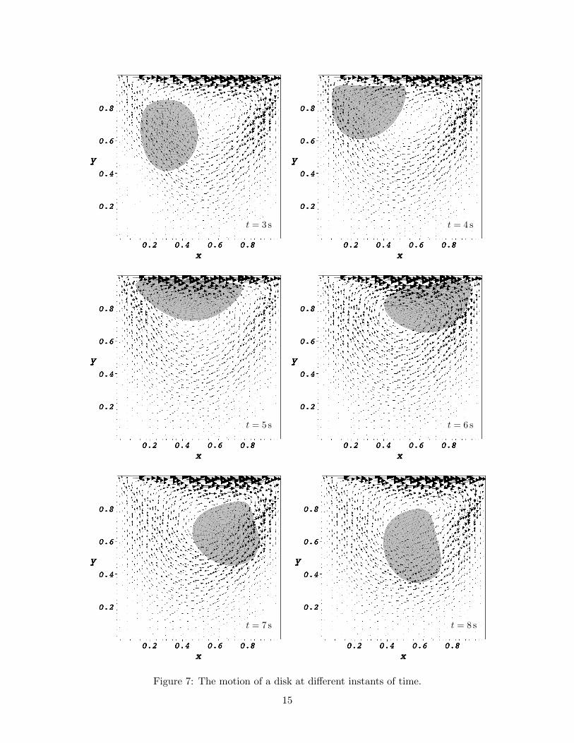
Figure 7: The motion of a disk at different instants of time.

15

Figure 8: Enlarged view of the disk depicting its shape and location at various instants of time.

Figure 9: (a) Percentage change in the area of the disk over time for the results shown in Fig. 7and 8. (b) Detail of plot (a) for three different refinement levels: Case 2 is the line in (a), whereasCases 1 and 3 have one level of refinement lower and higher than that in Case 2, respectively.

16

which can be shown to imply CD ∝ 1/Re (see, Jayaweera and Mason, 1965).Referring to Fig. 10, in our numerical experiments we consider a disk Bt (representing the

PseudocolorVar: p

x

y

VectorVar: v

Max: 0.000Min: 0.000

Max: 0.000Min: 0.000

1300

-1100

700

-500

100

0.2 0.4 0.6 0.8

1.5

1.0

0.5

x

y

0.46 0.50 0.54

0.12

0.08

0.04

0.16

Figure 10: Vertical channel containing viscous fluid through which a small incompressible disk isdescending: (a) system’s geometry; (b) initial conditions (disk released from rest in a quiescentfluid); (c) detail of mesh of the immersed body. The disk’s terminal velocity is denoted by Ut.

midplane of the cylinder), with radius R and center C, released from rest in an initially quiescentrectangular control volume Ω with height H and width W . As the disk sinks, we measure theposition of C and infer its velocity, denoted by uCy. When uCy achieves a (sufficiently) constantvalue, we refer to this value as the terminal velocity and denote it by UtN . When uCy = UtNwe also compute the drag coefficient CDN of the disk. The latter is assumed to consists of anincompressible neo-Hookean material whose Piola stress is given by

Ps = −psI +Ge(F− F−T

). (36)

The following parameters were used: H = 2.0 cm, W = 1.0 cm, R = 0.05 cm, ρf = 1.0 g/cm3,µs = 0, Ge = 1 × 103 dyn/cm2 and g = 981 cm/s2. Two different cases were considered. InCase 1, the density of the solid was varied while the viscosity of the fluid was held constant atµf = 1.0 P. In Case 2, we used for different fluid viscosities while the density of the solid was heldconstant at ρs = 3.0 g/cm3. The values used for ρs and µf can be found in Table 3, which also liststhe corresponding values of UtN , ReN , and CDtN . We have used Q2

0|Q10 elements for the control

volume and a Gauss quadrature rule of order 4 for assembling the operators defined over the soliddomain. In all numerical experiments pertaining to Cases 1 and 2, we have used 16,384 cells and181,250 DoFs for the control volume, and 320 cells and 2,626 DoFs for the solid.

The results for Case 1 are reported in Figs. 11 and 12, whereas those for Case 2 are reported

17

Table 3: Values of solid density and fluid density used for the tests. Also shown are the valuesobtained for the terminal velocity, Reynolds number and drag coefficient from these tests.

ρs(g/cm3) µf(P) UtN (cm/s) RetN CDtN

Case 12.0 1.0 0.8179 0.082 230.33.0 1.0 1.6270 0.163 116.44.0 1.0 2.4412 0.244 77.6

Case 2

3.0 1.0 1.6270 0.163 116.43.0 2.0 0.8236 0.041 454.43.0 4.0 0.4137 0.010 1801.03.0 8.0 0.2070 0.003 7192.5

(a) Axial position of mass center of the disk.

(b) Vertical velocity of mass center of the disk.

Figure 11: Effect of changing the density of the solid on the motion of the center of mass of thecylinder. Note: ρs1 = 2 g/cm3, ρs2 = 3 g/cm3 and ρs3 = 4 g/cm3.

(a) Velocity of mass center of the cylinder versustime.

(b) Terminal velocity of the cylinder as function ofits density

Figure 12: Effect of changing the density of the cylinder on its terminal velocity. Note: ρs1 =2 g/cm3, ρs2 = 3 g/cm3 and ρs3 = 4 g/cm3.

18

(a) Axial position of mass center of the disk.

(b) Vertical velocity of mass center of the disk

Figure 13: Effect of changing the viscosity of the fluid on the motion of the center of mass of thecylinder. Note: µf1 = 1.0 P, µf2 = 2.0 P, µf2 = 4.0 P and µf4 = 8.0 P.

(a) Velocity of mass center of the cylinder versus time.

(b) Terminal velocity of the cylinder as function of theviscosity of the fluid.

Figure 14: Effect of fluid viscosity on the terminal velocity of the disk. Note: µf1 = 1.0 P, µf2 =2.0 P, µf2 = 4.0 P and µf4 = 8.0 P.

19

in Figs. 13 and 4.2.3. Figures 11(b) and 13(b) show that uCy increases over a distance of abouty < H/3, remains constant over H/3 < y < 2H/3 and then decreases over the remaining length ofthe channel. This is in accordance with actual experimental observations (cf., Clift et al., 1978).From Figs. 12(a) and 14(a), we see that the disk’s terminal velocity increases with its density anddecreases with the increase in the fluid’s viscosity. Moreover, from Fig. 12(b) we see that theterminal velocity is linearly proportional to the density of the disk, and from Fig. 14(b) we see thatthe terminal velocity is inversely proportional to the viscosity of the fluid, as expected. Finally,from Fig. 15 we see that the calculated drag coefficient at the terminal velocity CDtN of the cylinder

Figure 15: Drag coefficient versus Reynolds number (corresponding to the terminal velocity of thecylinder).

is indeed inversely proportional to the corresponding Reynolds number RetN .We end this section with a few remarks on convergence and mesh refinement. The computed

value of the terminal velocity can be expected to be accurate only when the meshes are “sufficiently”refined. With this in mind, we considered the effect of mesh refinement on the the value of UtNfor Case 1 corresponding to ρs = 4 g/cm3. Table 4 shows the mesh sizes for both the solid and thecontrol volume along with the corresponding value of UtN . The corresponding velocity of C as a

Table 4: Terminal velocity of the cylinder obtained from simulations using meshes having differentglobal refinement levels.

Solid Control VolumeUtNcm/s

Cells DoFs Cells DoFs

Level 1 80 674 1,024 11,522 2.10Level 2 80 674 4,096 45,570 2.37Level 3 320 2,626 16,384 181,250 2.45Level 4 1,280 10,370 65,536 722,946 2.50

20

Figure 16: Effect of mesh refinement level on the terminal velocity of the mass center of the cylinder.

function of time is shown in Fig. 16, in which we see that, as the meshes are refined, UtN tends toachieve a “converged” value. We note that the Case 1 and 2 results presented earlier correspondto Level 3 in Table 4.

4.3 Results for Compressible Immersed Solids

4.3.1 Compressible Annulus inflated by a Point source

Here we present a problem involving a compressible solid with stress response containing bothelastic and viscous contributions. Specifically, we study the deformation of a hollow compressiblecylinder submerged in a fluid contained in a rigid prismatic box due to the influx of fluid along theaxis of the cylinder. Referring to Fig. 17, we consider a two-dimensional solid annulus with inner

Figure 17: Initial configuration of an annulus immersed in a square box filled with fluid. At thecenter C of the box is a point source of constant strength Q.

radius R and thickness w that is concentric with a fluid-filled square box of edge length l. A point

21

mass source of fluid of constant strength Q is located at the center C of Ω. Because of this source,the balance of mass for the system is modified as follows:∫

Ωq

[∇ · u+

Q

ρfδ(x− xC)

]v. −

∫Bt

q∇ · uv. = 0, (37)

where δ (x− xC) denotes a Dirac-δ distribution centered at C. We apply homogeneous Dirichletboundary conditions on ∂Ω. The annulus was chosen to have a compressible Neo-Hookean elasticresponse given by

Pes = Ge(F− J−2ν/(1−2ν)F−T

), (38)

where Ge is the elastic shear modulus and ν is the Poisson’s ratio for the solid. Since the solidis compressible both the volume of solid and that of the fluid in the control volume can change.However, since the fluid cannot leave the control volume, the amount of fluid volume increase mustmatch the decrease in the volume of the solid. This implies that the difference in these two volumescan serve as an estimate of the numerical error incurred.

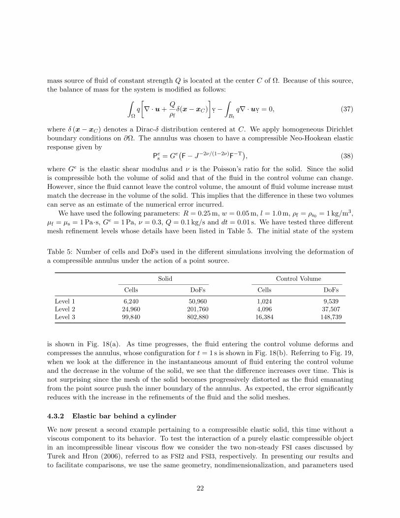
We have used the following parameters: R = 0.25 m, w = 0.05 m, l = 1.0 m, ρf = ρs0 = 1 kg/m3,µf = µs = 1 Pa·s, Ge = 1 Pa, ν = 0.3, Q = 0.1 kg/s and dt = 0.01 s. We have tested three differentmesh refinement levels whose details have been listed in Table 5. The initial state of the system

Table 5: Number of cells and DoFs used in the different simulations involving the deformation ofa compressible annulus under the action of a point source.

Solid Control Volume

Cells DoFs Cells DoFs

Level 1 6,240 50,960 1,024 9,539Level 2 24,960 201,760 4,096 37,507Level 3 99,840 802,880 16,384 148,739

is shown in Fig. 18(a). As time progresses, the fluid entering the control volume deforms andcompresses the annulus, whose configuration for t = 1 s is shown in Fig. 18(b). Referring to Fig. 19,when we look at the difference in the instantaneous amount of fluid entering the control volumeand the decrease in the volume of the solid, we see that the difference increases over time. This isnot surprising since the mesh of the solid becomes progressively distorted as the fluid emanatingfrom the point source push the inner boundary of the annulus. As expected, the error significantlyreduces with the increase in the refinements of the fluid and the solid meshes.

4.3.2 Elastic bar behind a cylinder

We now present a second example pertaining to a compressible elastic solid, this time without aviscous component to its behavior. To test the interaction of a purely elastic compressible objectin an incompressible linear viscous flow we consider the two non-steady FSI cases discussed byTurek and Hron (2006), referred to as FSI2 and FSI3, respectively. In presenting our results andto facilitate comparisons, we use the same geometry, nondimensionalization, and parameters used

22

PseudocolorVar: p

x

y

VectorVar: v

Max: 0.000Min: 0.000

Max: 0.000Min: 0.000

0.2 0.4 0.6 0.8

0.2

0.4

0.6

0.8

(a) t = 0 s

PseudocolorVar: p

x

y

VectorVar: v

Max: 2500Min: -680.2

Max: 2.765Min: 0.000

0.2 0.4 0.6 0.8

0.2

0.4

0.6

0.8

2500

-680.2

1705

114.8

909.9

(b) t = 1.0 s

Figure 18: The velocity and the mean normal stress field over the control volume. Also shown isthe annulus mesh.

Time (s)

δVs(m

3)

0 0.2 0.4 0.6 0.8 1−10

−9.5

−9

−8.5

−8

−7.5x 10−4

Level 1Level 2Level 3

Student Version of MATLAB

0 0.2 0.4 0.6 0.8 10

5

10

15

20

Time (s)

δVerr(%

)

Level 1Level 2Level 3

Student Version of MATLAB

Figure 19: The difference between the instantaneous amount of fluid entering due to the sourceand the change in the area of the annulus. The difference reduces with mesh refinement.

23

Figure 20: Solution domain for the problem of an elastic bar behind a cylinder.

by Turek and Hron (2006). Specifically, referring to Fig. 20, the system consists of a 2D channelof dimensions L = 2.5 m and height H = 0.41 m, with a fixed circle K of diameter d = 0.1 m andcentered at C = (0.2, 0.2) m. The elastic bar attached at the right edge of the circle has lengthl = 0.35 m and height h = 0.02 m.

The constitutive response of the bar is that of a de Saint-Venant Kirchhoff material (Holzapfel,2000; Turek and Hron, 2006) so that the viscous component of the stress is equal to zero (σvs = 0)and the (purely) elastic stress behavior is given by

σes = J−1F[2GeE + λe(trE)I

]FT = J−1F

[2GeE +

2Geνe

1− 2νe(trE)I

]FT, (39)

where E = (FTF − I)/2 is the Lagrangian strain tensor, Ge and λe are the Lame elastic constantsof the immersed solid, and where νe = λe/[2(λe +Ge)] is corresponding Poisson’s ratio.

The system is initially at rest. The boundary conditions are such that there is no slip overthe top and bottom surfaces of the channel as well as over the surface of the circle (the immersedsolid does not slip relative to the fluid). At the right end of the channel we impose “do nothing”boundary conditions. Using the coordinate system indicated in Fig. 20, at the left end of thechannel we impose the following distribution of inflow velocity:

ux = 1.5U 4y(H − y)/H2 and uy = 0, (40)

where U is a constant with dimension of speed.The constitutive parameters and the the parameter U used in the simulations are reported in

Table 6, in which we have also indicated the flow’s Reynolds number.

Table 6: Parameters used in the two non-steady FSI cases in Turek and Hron (2006).

Parameter FSI2 FSI3

ρs (103 kg/m3) 10.0 1.0νe 0.4 0.4Ge [106 kg/(m·s2)] 0.5 2.0ρf (103 kg/m3) 1.0 1.0µf (10−3 m2/s) 1.0 1.0U (m/s) 1.0 2.0ρs/ρf 10.0 1.0Re = Ud/µf 100.0 200.0

24

The outcome of the numerical benchmark proposed by Turek and Hron (2006) is typicallyexpressed (i) in terms of the time dependent position of the the midpoint A at the right end of theelastic bar, and (ii) in terms of the force acting on the boundary S of the union of the circle K andthe elastic bar Bt (see Fig. 21). Denoting by ı and the orthonormal base vectors associated with

Figure 21: Domain resulting from the union of the elastic bar Bt and the fixed circle K with centerC. S = ∂(K ∪ Bt) denotes the boundary of the domain in question and it is oriented by the unitnormal ν. Point A is the midpoint on the right boundary of the elastic bar.

the x and y axes, respectively, the force acting on the domain S is

FD ı+ FL =

∫Sσνa. , (41)

where FD and FL are the lift and drag, respectively, and where σν is the (time dependent) tractionvector acing on S. As remarked by Turek and Hron (2006) there are several ways to evaluate theright-hand side of Eq. (41). For example, the traction on the elastic bar could be calculated onthe fluid side or on the solid side or even as an average of these values.∗ However, we need to keepin mind that we use a single field for the Lagrange multiplier p and that this field is expected tobe discontinuous across the across the (moving) boundary of the immersed object. In turn, thismeans that the measure of the hydrodynamic force on S via a direct application of Eq. (41) wouldbe adversely affected by the oscillations in the field p across S. With this in mind, referring to thesecond of Eqs. (1), we observe that a straightforward application of the divergence theorem overthe domain Ω \ (K ∪Bt) yields the following result:

FD ı+ FL =

∫∂Ωσna. −

∫Ω\(K∪Bt)

ρ

b−

[∂u

∂t+ (∇u)u

]v. , (42)

where n denotes the outward unit normal of ∂Ω. The estimation of the lift and drag over S viaEq. (42) is significantly less sensitive to the oscillations of the field p near the boundary of theimmersed domain and this is the way we have measured FD and FL.

For both the FSI2 and FSI3 benchmarks, we performed calculations using 2,992 Q20|Q1

0 elementsfor the fluid and 704 Q2

0 elements for the immersed elastic bar. The number of degrees of freedomdistributed over the control volume is 24,464 for the velocity and 3,124 for the pressure. Thenumber of degrees of freedom distributed over the elastic bar is 6,018. The time step size for theFSI2 benchmark was set to 0.005 s, whereas the time step size for the FSI3 results was set to 0.001 s.

The results for the FSI2 case are shown in Figures 22 and 23 displaying the components of thedisplacement of point A and the components of the hydrodynamic force on S, respectively. Theanalogous results for the FSI3 case are displayed in Figs. 24 and 25. As can be seen in these

∗Ideally, the traction value computed on the solid and fluid sides are the same.

25

Figure 22: Nondimensional displacement of the midpoint at the right end of the elastic bar vs.time. The horizontal and vertical components of the displacement are plotted to the left and tothe right, respectively.

Figure 23: Plots of the lift (left) and drag (right) that the fluid exerts on the immersed fixedcylinder and the elastic bar.

figures, the displacement values as well as the lift and drag results compare rather favorably withthose in the benchmark proposed by Turek and Hron (2006), especially when considering that ourintegration scheme is the implicit Euler method.

4.4 Flexible 3D bar behind a prismatic rigid obstacle

Here we present some calculations pertaining to a simple three-dimensional problem. These resultsare not intended to reproduce any rigorous benchmarks. Rather, they provide a snapshot of ourcurrent computational capability, which consists of a serial code using UMFPACK (Davis, 2004)as a direct solver, rather than an optimized parallel code with a carefully designed pre-conditioner.In this sense, the results presented in this section point to the challenges we plan to tackle in thefuture. A simplified version of the software used to generate the results of this paper is availablein Heltai et al. (2014).

Benchmarks for three-dimensional FSI problems are not as established as those by Turek andHron for the two-dimensional cases. Due to the limitations of out current code, we chose the simplethree-dimensional problem found in Section 4.4 of the paper by Wick (2011). Referring to Fig. 26,we consider the motion of an elastic bar attached to a rigid prismatic obstacle across a channel.Both the channel and the obstacle have square crossections. The obstacle and the elastic bar are

26

Figure 24: Nondimensional displacement of the midpoint at the right end of the elastic bar vs.time. The horizontal and vertical components of the displacement are plotted to the left and tothe right, respectively.

Figure 25: Plots of the lift (left) and drag (right) that the fluid exerts on the immersed fixedcylinder and the elastic bar.

not symmetrically located along the y direction within the channel. In addition, the elastic baris not positioned symmetrically within the channel along the z direction. The dimensions of thechannel, the rigid obstacle, and the elastic bar attached to the obstacle are shown in the figure. Thestress behavior is purely elastic of the type indicated in Eq. (39). The parameters in the simulationare chosen as follows: ρf = 1.0 kg·m−3, µf = 0.01 m2/s, ρs = 1.0 kg·m−3, Ge = 500 kg/(m·s2) andνe = 0.4. A constant parabolic velocity profile is prescribed at the inlet:

ux(0, y, z, t) = 16Uyz(H − y)(H − z)H−4, uy(0, y, z, t) = 0, uz(0, y, z, t) = 0, (43)

where H = 4.1 m and U = 0.45 m/s. At the outlet “do nothing” boundary conditions are imposed.The quantities monitored during the calculations are the components wx, wy, and wz of the dis-placement of point A(t), as well as the drag and lift around the obstacle and the elastic bar. Thecoordinates of A at the initial time are (8.5, 2.5, 2.73) m.

Referring to Table 7, we have considered two types of discretization, one isotropic and oneanisotropic. For each we considered two levels of refinement. Although our code can cope withup to three refinement levels, the solution at each time step for refinement levels higher than tworequires several hours of computing time, rendering such grids impractical for unsteady simulations.

27

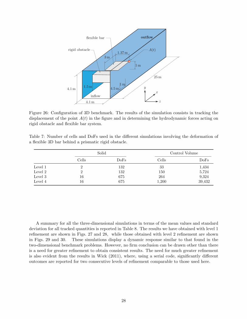
Figure 26: Configuration of 3D benchmark. The results of the simulation consists in tracking thedisplacement of the point A(t) in the figure and in determining the hydrodynamic forces acting onrigid obstacle and flexible bar system.

Table 7: Number of cells and DoFs used in the different simulations involving the deformation ofa flexible 3D bar behind a prismatic rigid obstacle.

Solid Control Volume

Cells DoFs Cells DoFs

Level 1 2 132 33 1,434Level 2 2 132 150 5,724Level 3 16 675 264 9,324Level 4 16 675 1,200 39,432

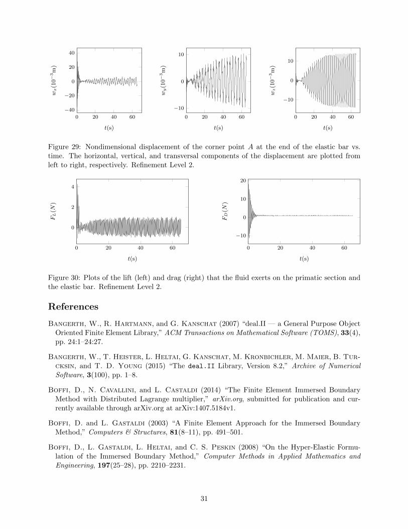
A summary for all the three-dimensional simulations in terms of the mean values and standarddeviation for all tracked quantities is reported in Table 8. The results we have obtained with level 1refinement are shown in Figs. 27 and 28, while those obtained with level 2 refinement are shownin Figs. 29 and 30. These simulations display a dynamic response similar to that found in thetwo-dimensional benchmark problems. However, no firm conclusion can be drawn other than thereis a need for greater refinement to obtain consistent results. The need for much greater refinementis also evident from the results in Wick (2011), where, using a serial code, significantly differentoutcomes are reported for two consecutive levels of refinement comparable to those used here.

28

Table 8: Mean and standard deviation values of the components of the displacement of A(t) as wellas of the lift and drag over time and as a function of the refinement level.

Level Time interval size (s)

10 20 60 80

wx: (mean, std)× 103 m 1 0.269, 21.1 0.544, 15.4 0.977, 9.10 1.38, 8.15

2 0.370, 8.77 0.315, 6.32 0.126, 4.37 —3 1.86, 12.9 2.13, 9.14 — —4 0.463, 7.37 — — —

wy: (mean, std)× 103 m 1 0.00849, 2.08 0.865, 2.04 2.18, 4.71 2.16, 6.16

2 0.103, 1.07 0.0744, 1.89 0.333, 4.23 —3 -1.28, 1.34 -1.60, 1.83 — —4 -0.0699, 1.20 — — —

wz: (mean, std)× 103 m 1 -0.857, 2.50 -1.50, 1.97 -2.66, 4.70 -2.24, 5.63

2 0.0704, 1.26 -0.176, 3.61 -0.0857, 7.68 —3 -1.09, 1.51 -1.26, 1.08 — —4 0.0308, 0.758 — — —

FL: (mean, std) N 1 0.00424, 1.59 0.0334, 1.32 0.0175, 0.962 0.0138, 0.849

2 0.0264, 1.08 0.0317, 0.869 0.0407, 0.733 —3 0.00222, 0.481 0.00633, 0.373 — —4 0.0264, 1.08 — — —

FD: (mean, std) N 1 2.65, 82.7 2.06, 58.5 1.62, 33.8 1.58, 29.2

2 1.73, 47.9 1.34, 33.9 1.07, 19.6 —3 1.83, 35.9 1.43, 25.4 — —4 1.56, 30.2 — — —

29

0 20 40 60

−50

0

50

t(s)

wx(10−3m)

0 20 40 60

−10

0

10

t(s)

wy(10−3m)

0 20 40 60

−10

0

10

t(s)

wz(10−3m)

Figure 27: Nondimensional displacement of the corner point A at the end of the elastic bar vs.time. The horizontal, vertical, and transversal components of the displacement are plotted fromleft to right, respectively. Refinement Level 1.

0 20 40 60

−2

0

2

t(s)

FL(N

)

0 20 40 60

−20

0

20

t(s)

FD(N

)

Figure 28: Plots of the lift (left) and drag (right) that the fluid exerts on the primatic section andthe elastic bar. Refinement Level 1.

5 Summary and Conclusions

In this paper we have presented the first set of results meant to provide a validation of the fully vari-ational FEM approach to an immersed method for FSI problems presented in Heltai and Costanzo(2012). The most important result shows, for the first time, that our proposed immersed methodcan satisfy the rigorous benchmark tests by Turek and Hron (2006). Our results also show that theproposed approach can be applied to a wide variety of problems in which the immersed solid neednot have the same density or the same viscous response as the surrounding fluid. Furthermore,as shown by the results concerning the lid cavity problem, the proposed computational approachcan be applied to problems with very large deformations without any need to adjust the meshesused for either the control volume or the immersed solid. In the future, we plan to extend theseresults to include comparative analyses with more established ALE schemes and more extensiveand rigorous three-dimensional tests.

Acknowledgements

The research leading to these results has received specific funding within project OpenViewSHIP,”Sviluppo di un ecosistema computazionale per la progettazione idrodinamica del sistema elica-carena”, supported by Regione FVG - PAR FSC 2007-2013, Fondo per lo Sviluppo e la Coesione.

30

0 20 40 60

−40

−20

0

20

40

t(s)

wx(10−3m)

0 20 40 60

−10

0

10

t(s)

wy(10−3m)

0 20 40 60

−10

0

10

t(s)

wz(10−3m)

Figure 29: Nondimensional displacement of the corner point A at the end of the elastic bar vs.time. The horizontal, vertical, and transversal components of the displacement are plotted fromleft to right, respectively. Refinement Level 2.

0 20 40 60

0

2

4

t(s)

FL(N

)

0 20 40 60

−10

0

10

20

t(s)

FD(N

)

Figure 30: Plots of the lift (left) and drag (right) that the fluid exerts on the primatic section andthe elastic bar. Refinement Level 2.

References

Bangerth, W., R. Hartmann, and G. Kanschat (2007) “deal.II — a General Purpose ObjectOriented Finite Element Library,” ACM Transactions on Mathematical Software (TOMS), 33(4),pp. 24:1–24:27.

Bangerth, W., T. Heister, L. Heltai, G. Kanschat, M. Kronbichler, M. Maier, B. Tur-cksin, and T. D. Young (2015) “The deal.II Library, Version 8.2,” Archive of NumericalSoftware, 3(100), pp. 1–8.

Boffi, D., N. Cavallini, and L. Castaldi (2014) “The Finite Element Immersed BoundaryMethod with Distributed Lagrange multiplier,” arXiv.org, submitted for publication and cur-rently available through arXiv.org at arXiv:1407.5184v1.

Boffi, D. and L. Gastaldi (2003) “A Finite Element Approach for the Immersed BoundaryMethod,” Computers & Structures, 81(8–11), pp. 491–501.

Boffi, D., L. Gastaldi, L. Heltai, and C. S. Peskin (2008) “On the Hyper-Elastic Formu-lation of the Immersed Boundary Method,” Computer Methods in Applied Mathematics andEngineering, 197(25–28), pp. 2210–2231.

31

Brenner, H. (1962) “Effect of Finite Boundaries on the Stokes Resistance of an Arbitrary Parti-cle,” Journal of Fluid Mechanics, 12(01), pp. 35–48.

Brezzi, F. and M. Fortin (1991) Mixed and Hybrid Finite Element Methods, vol. 15 of SpringerSeries in Computational Mathematics, Springer-Verlag, New York.

Clift, R., J. R. Grace, and M. E. Weber (1978) Bubbles, Drops, and Particles, AcademicPress, New York.

Davis, T. A. (2004) “Algorithm 832: UMFPACK V4.3—An Unsymmetric-Pattern MultifrontalMethod,” ACM Transactions on Mathematical Software (TOMS), 30(2), pp. 196–199.

Fai, T. G., B. E. Griffith, Y. Mori, and C. H. Peskin (2014) “Immersed Boundary Methodfor Variable Viscosity and Variable Density Problems Using Fast Constant-Coefficient LinearSolvers II: Theory,” SIAM Journal on Scientific Computing, 36(3), pp. B589–B621.

Griffith, B. E. (2012) “On the Volume Conservation of the Immersed Boundary Method,” Com-munications in Computational Physics, 12(2), pp. 401–432.

Griffith, B. E. and X. Luo (2012) “Hybrid Finite Difference/Finite Element Version of theImmersed Boundary Method,” International Journal for Numerical Methods in Engineering,submitted for publication.

Heltai, L. (2006) The Finite Element Immersed Boundary Method, Ph.D. thesis, Universita diPavia.

——— (2008) “On the Stability of the Finite Element Immersed Boundary Method,” Computers& Structures, 86(7–8), pp. 598–617.

Heltai, L. and F. Costanzo (2012) “Variational Implementation of Immersed Finite ElementMethods,” Computer Methods in Applied Mechanics and Engineering, 229–232, pp. 110–127,DOI: 10.1016/j.cma.2012.04.001.

Heltai, L., S. Roy, and F. Costanzo (2014) “A Fully Coupled Immersed Finite Element Methodfor Fluid-Structure Interaction via the Deal.II Library,” Archive of Numerical Software, 2(1), pp.1–27.

Holzapfel, G. A. (2000) Nonlinear Solid Mechanics, John Wiley & Sons, Ltd., Chichester.

Jayaweera, K. O. L. F. and B. J. Mason (1965) “The Behaviour of Freely Falling Cylindersand Cones in a Viscous Fluid,” Journal of Fluid Mechanics, 22(04), pp. 709–720.

Peskin, C. S. (1977) “Numerical Analysis of Blood Flow in the Heart,” Journal of ComputationalPhysics, 25(3), pp. 220–252.

——— (2002) “The Immersed Boundary Method,” Acta Numerica, 11, pp. 479–517.

Turek, S. and J. Hron (2006) “Proposal for Numerical Benchmarking of Fluid-Structure Interac-tion Between an Elastic Object and Laminar Incompressible Flow,” in Fluid-Structure Interaction(H.-J. Bungartz and M. Schafer, eds.), vol. 53 of Lecture Notes in Computational Science andEngineering, Springer, Berlin, Heidelberg, pp. 371–385, DOI: 10.1007/3-540-34596-5 15.

Wang, X. and W. K. Liu (2004) “Extended Immersed Boundary Method using FEM and RKPM,”Computer Methods in Applied Mechanics and Engineering, 193(12–14), pp. 1305–1321.

32

Wang, X. and L. Zhang (2010) “Interpolation Functions in the Immersed Boundary and FiniteElement Methods,” Computational Mechanics, 45, pp. 321–334.

Wick, T. (2011) “Fluid-Structure Interactions using Different Mesh Motion Techniques,” Com-puters and Structures, 89(13–14), pp. 1456–1467.

Zhang, L., A. Gerstenberger, X. Wang, and W. K. Liu (2004a) “Immersed Finite ElementMethod,” Computer Methods in Applied Mechanics and Engineering, 193(21–22), pp. 2051–2067.

Zhang, L. T. and M. Gay (2007) “Immersed Finite Element Method for Fluid-Structure Inter-actions,” Journal of Fluids and Structures, 23(6), pp. 839–857.

Zhang, L. T., A. Gerstenberger, X. Wang, and W. K. Liu (2004b) “Immersed Finite ElementMethod,” Computer Methods In Applied Mechanics and Engineering, 193(21-22), pp. 2051–2067.

33