Demand Estimation Model Sensitivity Analysis

Demand Estimation Model Sensitivity AnalysisGary B. Lauson, M.S., P.E.

February 17, 2016

Abstract

In response to the classic problem of balancing Inventory Investment with Service Level, a numericalmodel was developed within Arris to estimate /forecast inventory demand one month into the future. Anumerical approach was selected because it was perceived that traditional Statistical methods weresuboptimal for estimating inventory demand. The author developed a Numerical Demand EstimationModel that is designed to approximate human Demand Planning /forecasting judgment. This paperdetermined that the numerical model provides inventory management advantages over two traditionalStatistical approaches to demand estimation: (A) the Three-Month Simple Moving Average (3M MA),and, (B) the Six-Month Simple Moving Average (6M MA). However, the advantages come with thesacrifice of a portion of the Service Level that is provided by Moving Averages. A computer simulation ofinventory behavior was developed to evaluate the performance of the Numerical Model relative to thecapabilities of the 3M and 6M MAs. Tables of sensitivity /performance data for the three models areprovided in the "Model Sensitivity" Section of the paper (page five). These tables provide informationwhich allow the reader to draw conclusions on the relative utility of the three models that were evaluated.

Model Purpose

A critical goal of Inventory Management is the achievement of an effective balance between InventoryInvestment and Service Level. In 2015, a Numerical Demand Estimation Model was substantiallycompleted within the Supplies Division. The model was designed to help Supplies achieve the abovegoal by satisfying the following objectives:

1. Computerized approximation of Demand Planner judgment used to estimate the next future month'scustomer demand from available historical demand data.

2. Utilization of the above demand estimates to compute two key Material Requirements Planning(MRP) parameters: (a) Reorder Point, and (b) Economic Order Quantity. (MRP is the automatedsystem used in Supply Chain to sequence and control inventory ordering.)

3. To the extent reasonable, make customers pull inventory from Arris; i.e., improve inventory efficiencyby further incorporating "demand-driven supply" principles into the Supplies Division (Mendes, p.5,2011). Note that this philosophy requires regular monitoring of inventory-level action signals.Custom computer programs were developed and put in place to facilitate the monitoring.

Although a functional numerical model was developed and peer reviewed, the sale of Supplies toTechnetix did not allow the model to be optimized or put into service.

Model Description

Because of the popularity of Excel within Arris, the Demand Estimation Model was developed inVBA/Excel. (VBA stands for "Visual BASIC for Applications," and is a programming language includedwith every Microsoft application program.) The model estimates customer demand as follows:

1. The operator specifies the desired Confidence Level of the Demand Estimate; e.g., 90-percent, 95-

percent, etc.

2. The program determines if there are high-probability outlier demand conditions, such as past demandspikes or a current demand surge. The program then suppresses these conditions to arrive at a dataset that represents a temporal demand distribution that will likely continue into the future (again, in aneffort to approximate Demand Planner judgment).

3. The program then regresses a line across 12 months of probable historical data. The slope of theresulting line provides an estimate of the trend within the data. The 12-month period was selectedbecause it allows the program to be used for both short- and long-lead time items.

4. The program then applies a complex combination of Root Location, Integration, and Line IntersectionIdentification procedures to adjust the vertical position of the regressed line (without changing itsslope) such that the specified Confidence Level Demand Estimate is reached. Numerical Integrationenables the program to operate on the classic statistics concept that probability is equivalent to thearea under a probability distribution curve. In this case, the historical demand provides atemporal /probable demand distribution curve.

5. The program then estimates the next-month's demand from the computed position of the regressedline.

6. Additional situation-specific, judgment-based procedures are applied to finalize the demand estimate.

7. Through the following simple relationships, the demand- and lead-time-associated Safety Stock andReorder Point Inventory Levels are computed.

Dso = 50%-Probable Demand

D9s = 95%-Probable Demand

SS = (Ds5 — D5o) *Lead Time = Safety Stock Inventory Level

ROP = D5o *Lead Time + SS = Reorder Point Inventory Level

Note 1: From the perspective of the model, Safety Stock is defined as the inventory level required toraise Service Level performance from 50 percent to the operator-specified Confidence Level(typically 95 percent). This segregation of Inventory Levels into Safety Stock and Lead-TimeStock provides an estimate of the insurance (i.e., cost) required to move from Average Serviceto the desired Service Level.

Note 2: Seasonality estimation was not incorporated into the program's evaluation of time seriesdemand. Fourier Analysis is the likely approach for seasonality estimation; but it would probablybe best to apply it to 18-24 months' data.

Inventory Simulation

To evaluate the performance of the Demand Estimation Model (including its Sensitivity), a ReOrder-Point-based Inventory Simulation Program was developed in VBA/Excel. Following are the importantaspects of the program.

A. It utilizes actual demand on 197 Purchased-Finished Goods (PFG) items from Supplies shipping

2/12

history. (This decision imposes areal-world condition on the simulation and permits accurate modelerror assessment.)

B. The test forecast period is 12 months (2014) with the simulation starting 1/1/2014 with inventory atthe Reorder Point and concluding on 12/31/2014.

C. 200 PFG items were selected. Three (3) items were removed from the trial because they producedprogram run-time errors. These kinds of errors are a normal part of program development; they willbe investigated and eliminated.

D. Supplies' data was used because of the author's familiarity with it.

E. The Reorder Point method was simulated because it is the only Demand Planning Method in whichthe author has received training. if necessary, other Demand Planning Methods can be programmedfor simulation.

F. The Simulation Program calls the Demand Estimation Model. In other words, the SimulationProgram is a test program, separate from the Demand Estimation Model.

G. The question of sensitivity is really a question of the inventory overages and shortages that can beexpected. An inventory simulation was deemed the best means for evaluating different aspects ofDemand Estimation Model sensitivity.

H. Lead time variation was not included in the simulation.

I. Order minimums and multiples were not included in the simulation because this helps isolateDemand Estimation Method efficiencies, making them as apparent as possible.

Inclusion of a 30-day Economic Order Quantity. This means that when the Reorder Point isreached, the program orders enough for 30-days' demand beyond the Reorder Point; therebyimposing once-a-month ordering.

K. In comparing the performance of the Numerical Model with the Moving Average (MA) Models, itneeds to be recognized that the MA Models account for demand variation through the Normal

Distribution's application of the standard deviation (recall the 95-percent Confidence Level z-score =1.64). For small sample sizes, the correct probability distribution to use is the more conservativeStudent's tDistribution — however, this is rarely done in Supply Chain calculations because of theattendant increase in inventory. For example, if we apply the 95-percent Confidence Level and theStudents t Distribution, the 3M MA demand variation increases by 78 percent (t-score = 2.92 vs. z-score = 1.64), and the 6M MA demand variation increases by 22 percent (t-score = 2.015 vs. z-score= 1.64). Additionally, the simulation program applies a biased computation of the standard deviation(rather than the unbiased (n — 1) version). This is because the unbiased equation is rarely used inSupply Chain standard deviation calculations.

The Simulation Program computes and works with the following key variables (note that these variablesare the basis for addressing the question of model sensitivity).

1. Service Level (Annual).

2. Inventory Investment (per-month average).

3. Order Frequency (per-month average).

3/12

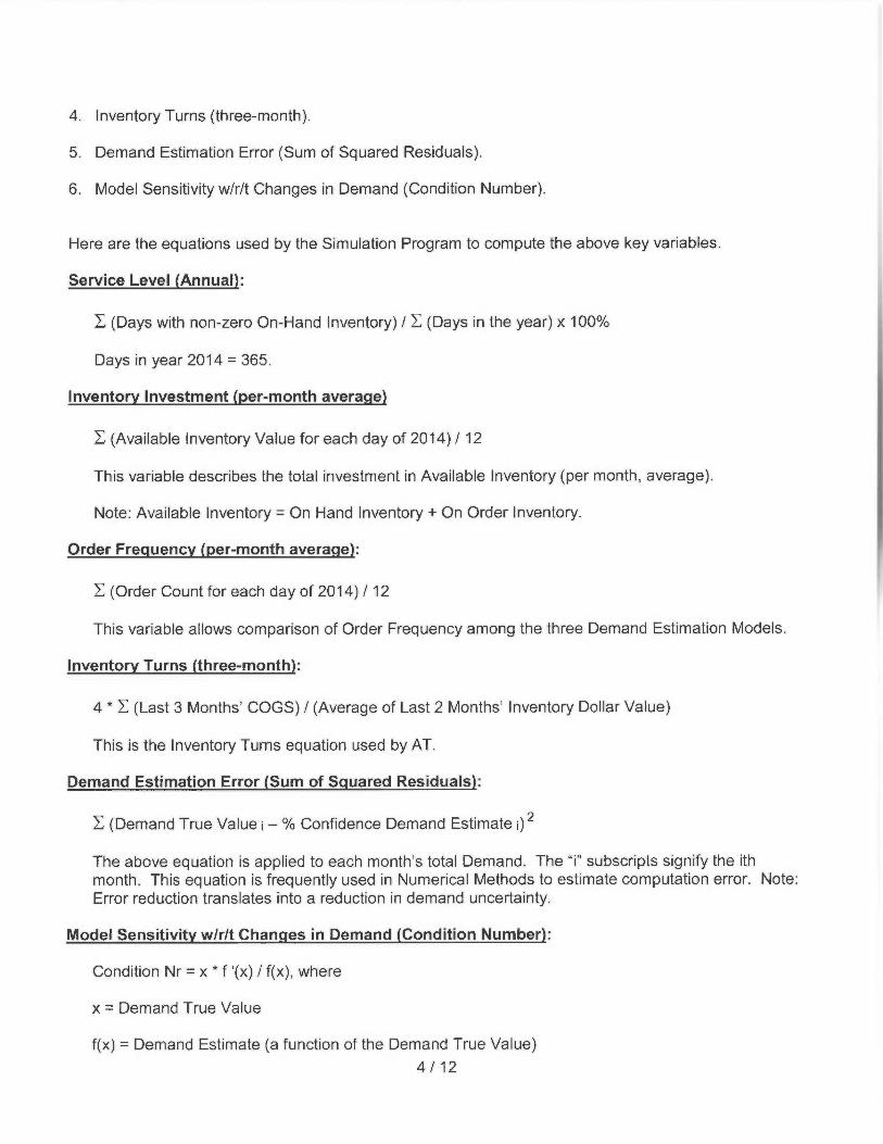
4. Inventory Turns (three-month).

5. Demand Estimation Error (Sum of Squared Residuals).

6. Model Sensitivity w/r/t Changes in Demand (Condition Number).

Here are the equations used by the Simulation Program to compute the above key variables.

Service Level (Annual):

~ (Days with non-zero On-Hand Inventory) / ~ (Days in the year) x 100%

Days in year 2014 = 365.

Inventory Investment (per-month average)

~ (Available Inventory Value for each day of 2014) / 12

This variable describes the total investment in Available Inventory (per month, average).

Note: Available Inventory = On Hand Inventory + On Order Inventory.

Order Frequency (per-month average):

~ (Order Count for each day of 2014) / 12

This variable allows comparison of Order Frequency among the three Demand Estimation Models.

Inventory Turns (three-month):

4 * ~ (Last 3 Months' COGS) / (Average of Last 2 Months' Inventory Dollar Value)

This is the Inventory Turns equation used by AT.

Demand Estimation Error (Sum of Squared Residuals):

~ (Demand True Value i — %Confidence Demand Estimate i) 2

The above equation is applied to each month's total Demand. The "i" subscripts signify the ithmonth. This equation is frequently used in Numerical Methods to estimate computation error. Note:Error reduction translates into a reduction in demand uncertainty.

Model Sensitivity w/r/t Changes in Demand (Condition Number):

Condition Nr = x '` f '(x) / f(x), where

x = Demand True Value

f(x) = Demand Estimate (a function of the Demand True Value)

4/12

f '(x) =First Derivative of the Demand Estimate (e.g., the 95-percent Confidence Level Estimate)

The above equation is found in Chapra/Canale's fourth edition of "Numerical Methods for Engineers."The first derivative that forms part of the above equation is numerically estimated as follows:

f ̀ (x) _ (f(x;+,) — f(x;-,) / (2 * Ox) (Chapra/Canale, p.93, 2002).

Sensitivity is a measure of "how a system responds under different conditions" (Chapra/Canale, p.21,2002). And the "condition of a mathematical problem relates to its sensitivity to changes in its inputvalues" (Chapra/Canale, p.92, 2002). Thus, the Condition Number provides a recognized calculationof Sensitivity, and permits quantified comparison of Sensitivity among the three Demand EstimationModels considered in this paper.

Model Sensitivity

The tables in this section compare the simulated performance of the three Demand Estimation Models(the 3M Moving Average, the 6M Moving Average, and the Numerical Method). The last row of eachcomparison is titled "SL Marginal Cost ($ / %)"; this stands for Service Level Marginal Cost (i.e., the pricepaid for the estimated change in Service Level with respect to the Numerical Model).

SL Marginal Cost = Change (Investment Sum) /Change (Service Level)

Improved performance (of a Moving Average Model relative to the Numerical Model) is identified bygreen-shaded cells. Deteriorated performance is identified by yellow-shaded cells. For the definitionsand equations used to compute each variable, see the section titled "Inventory Simulation." Thetabulated data from which the data in Tables One through Five are constructed is contained in Table Six.

Table One: 95- ercent Confidence Level N = 197Model: 3M MA 6M MA Numerical Model NM

Service Level SL % 83.2 89.4 86.4Investment Sum $ / Mo 50,262,395 48,250,934 34,248,125Order Fre /Item

/ Mo 0.56 0.68 0.83Turns 2.3 2.6 5.1Demand Error w/r/t NM 147% Increase 192% Increase N/ASensitivit w/r/t NM 186% Increase 44% Increase * N/ASL Mar final Cost 0$ / 0% -5,004,459 4,667,603 N/A* The 44 percent increase in Sensitivity is an improvement because of the increase in Service Level.

Table Two: 90-percent Confidence Level (N = 197)Model: 3M MA 6M MA Numerical Model (NM)

Service Level SL % 82.1 88.2 83.5Investment Sum $ / Mo 45,325,423 43,476,275 29,129,478Order Fre /Item

/

Mo 0.55 0.68 0.79Turns 2.6 3.1 6.5Demand Error w/r/t NM 147% Increase 187% Increase N/ASensitivit w/r/t NM 143% Increase 19% Increase * N/ASL Mar final Cost 4$ / O% -11,568,532 3,052,510 N/A* The 19 percent increase in Sensitivity is an improvement because of the increase in Service Level.

5/12

Table Three: 85-percent Confidence Level (N = 197)Model: 3M MA 6M MA Numerical Model NM

Service Level SL % 81.3 87.5 80.6Investment Sum $ / Mo 42,055,982 40,129,384 26,212,896Order Fre /Item

/ Mo 0.55 0.65 0.74Turns 3.0 3.5 7.4Demand Error w/r/t NM 118% Increase 150% Increase N/ASensitivit w/r/t NM 113% Increase 2% Increase N/ASL Mar final Cost 4$ / 4% 22,632,980 2,016,882 N/A* The 2 percent increase in Sensitivity is an improvement because of the increase in Service Level.

Table Four: 80- ercent Confidence Level N = 197Model: 3M MA 6M MA Numerical Model NM

Service Level SL % 80.6 86.6 78Investment Sum $ / Mo 39,676,025 37,437,926 24,069,417Order Fre /Item

/ Mo 0.54 0.64 0.69Turns 3.3 4.0 8.1Demand Error w/r/t NM 83% Increase 106% Increase N/ASensitivit w/r/t NM 89% Increase -11 %Decrease N/ASL Mar final Cost 4$ / D% 6,002,542 1,554,478 N/A* The 11 percent decrease in Sensitivity is an improvement because of the increase in Service Level.

Table Five: 75-percent Confidence Level (N = 197)Model: 3M MA 6M MA Numerical Model NM

Service Level SL % 79.5 85.7 75.1Investment Sum $ / Mo 37,710,361 35,323,398 21,871,086Order Fre /Item / Mo 0.53 0.63 0.65Turns 3.6 4.5 9.0Demand Error w/r/t NM 49% Increase 66% Increase N/ASensitivit w/r/t NM 237% Increase -22% Decrease N/ASL Mar final Cost O$ / 4% 3,599,835 1,269,086 N/A* The 22 percent decrease in Sensitivity is an improvement because of the increase in Service Level.

6/12

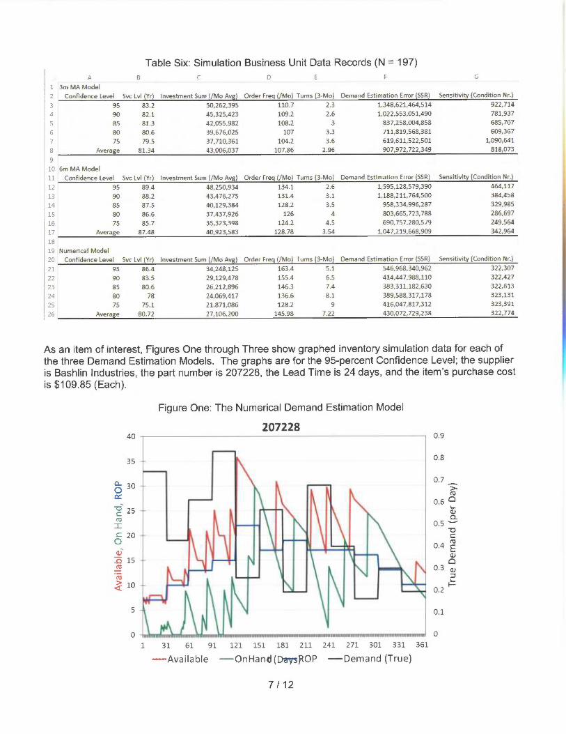
Table Six: Simulation Business Unit Data Records (N = 197)

A B C ~ E F G

1 3m MA Model

2 Confidence Level Svc Lvl (Yr) Investment Sum (/Mo Avg) Order freq (/Mo) Tums (3-Mo) Demand Estimation Error (SSR) Sensitivity (Condition Nr.)

3 95 83.2 50,262,395 110.7 2.3 1,348,621,464,514 922,714

4 90 82.1 45,325,423 109.2 2.6 1,022,553,051,490 781,937

S 85 81.3 42,055,982 108.2 3 837,258,004,858 685,707

6 80 80.6 39,676,025 107 3.3 711,819,568,381 609,367

7 75 79.5 37,710,361 104.2 3.6 619,611,522,501 1,090,641

8 Average 81.34 43,006,037 107.86 2.96 907,972,722,349 818,073

9

10 6m MA Model

11 Confidence Level Svc Lvl (Yr) Investment Sum (/Mo Avg) Order Freq (/Mo) Turns (3-Mo) Demand Estimation Error (SSR) Sensitivity (Condition Nr.)

12 95 89.4 48,250,934 134.1 2.6 1,595,128,579,390 464,117

13 90 88.2 43,476,275 131.4 3.1 1,188,211,764,500 384,458

14 85 87.5 40,129,384 128.2 3.5 958,334,996,287 329,985

15 80 86.6 37,437,926 126 4 803,665,723,788 286,697

16 75 85.7 35,323,398 124.2 4.5 690,757,280,579 249,564

17 Average 87.48 40,923,583 128.78 3.54 1,047,219,668,909 342,964

18

19 Numerical Model

20 Confidence Level Svc Lvl (Yr) Investment Sum (/Mo Avg} Order Freq (/Mo) Turns (3-Mo) Demand Estimation Error (SSR) Sensitivity (Condition Nr.)

21 95 86.4 34,248,125 163.4 5.1 546,968,340,962 322,307

22 90 83.5 29,129,478 155.4 6.5 414,447,988,110 322,427

23 85 80.6 26,212,896 146.3 7.4 383,311,182,630 322,613

24 80 78 24,069,417 136.6 8.1 389,588,317,178 323,131

25 75 75.1 21,871,086 128.2 9 416,047,817,312 323,391

26 Average 80.72 27,106,200 145.98 7.22 430,072,729,238 322,774

As an item of interest, Figures One through Three show graphed inventory simulation data for each ofthe three Demand Estimation Models. The graphs are for the 95-percent Confidence Level; the supplieris Bashlin Industries, the part number is 207228, the Lead Time is 24 days, and the item's purchase costis $109.85 (Each).

40

~~y

~ 30

~ 25

Z~ 20Oa.~ 15

caQ 1~

5

V

Figure One: The Numerical Demand Estimation Model

207228

1 31 61 91 121 151 181 211 241 271 301 331 361

-Available -OnHand (DagsROP -Demand (True)

7/12

0.9

0.8

.~

0.6 ~vn

0.5 "'

c0.4 ~

vD

0.3 ~

L

~.Z

0.1

0

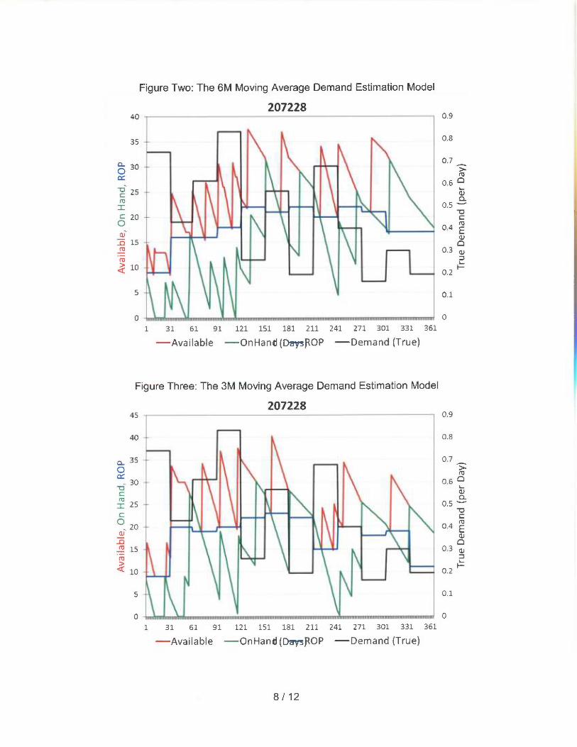
Figure Two: The 6M Moving Average Demand Estimation Model

ao 207228

35

~ 30

~ 25

S

~ 20O

v~ 15

caQ 10

5

0 ~

1

0.9

0.8

0.7

0.6 ~a`~Q

0.5 "'

c0.4 ~

vD

0.3 ~

L

~.Z

0.1

0

31 61 91 121 151 181 211 241 271 301 331 361

—Available —OnHand (Da~q~sROP —Demand (True)

Figure Three: The 3M Moving Average Demand Estimation Model

20722845

C[~l

~ 35

C~

30

c= 25

Q 10

5

0

1

0.9

0.8

0.7

0.6 ~

va

0.5 ̀ -'

c0.4 ~

D0.3 ~

L

~.2

0.1

0

31 61 91 121 151 181 211 241 271 301 331 361

—Available —OnHand (Daq~sROP —Demand (True)

8/12

Conclusions

• The superior accuracy of the Numerical Demand Estimation Model comes at the expense of afraction of the Service Level that accompanies the Moving Average Models.

• The Simulation Program developed to support this paper could be very useful for optimizing aDemand Estimation Model's performance for the demand patterns the model will encounter.

• Simulation can reduce, but not eliminate, the time and risk of involving business operations in theoptimization of complex processes.

• Applying a Numerical Demand Estimation Model to inventory operations carries the added potentialbenefit of identifying excessive and inadequate inventory conditions. The idea is to use the model toperiodically generate early-warning decision-support inventory action signals. The model (throughsimulation) may even have utility for the optimization of product families and a variety of otheraspects of inventory management.

• If the Numerical Demand Estimation Model is placed into service, improvement of its ability to identifyand effectively respond to a variety of demand patterns will be needed. In other words, all sources oferror in the model need to be identified and mitigated.

• A numerical approach to solving quantitative problems provides the significant benefit of being ableto include IF-THEN decision criteria in the solution.

• Inventory turns appear to be, in part, a function of: (1) Moving Average span (i.e., three-month, six-month, etc.), and (2) the confidence level selected for the standard deviation computation thataccompanies use of the Moving Average.

Additional Investigative Questions

In exploring Demand Estimation Model Sensitivity, it came to mind that answers to the followingadditional questions may yield inventory management benefits for Arris.

1. How are Inventory Turns related to: (a) Demand Estimation Confidence Level, (b) Economic OrderQuantity, and (c) Lead Time?

2. How is Service Level related to: (a) Demand Estimation Confidence Level, (b) Economic OrderQuantity, and (c) Lead Time?

3. What is the relationship between Inventory Turns and Service Level?

4. How well does the Numerical Demand Estimation Model perForm when compared with ExponentialMoving Averages? (Note that this paper investigated Simple Moving Averages.)

Lastly, although this project was assembled and validated with great care, programming the solution tocomplex problems always incurs the chance for error. Nevertheless, the work product described andprovided in this paper is believed to be accurate and unbiased. If I become aware of error in the work,will investigate it and make needed changes to the conclusions of this paper.

9/12

Please let me know if I can answer any questions on the information provided, or if additional informationis desired.

,,aa~,iuiuNh~

~r.,ra .~ g. l.,qL.•, fi~~,.~ ~

O`~,~^`s

2~~120~~0 = ~ Z` _

Gary B. Lauson, M.S., P.E. -~ ; ~~,g7F, ~ _~

Business Operations Manager, Arris %9<,,;+,y ,,~.~~''> ~r~, , . ~ ,.. ,

ar r

10 / 12

Bibliography

Chapra, Steven C. and Canale, Raymond P. Numerical Methods for Engineers, Fourth EditioMcGraw Hill, 2002.

Mendes, Paulo Demand Driven Supply Chain, Berlin Heidelberg: Springer-Verlag, 2011.

11 / 12

Numerical Methods Vita

For 14 years Gary Lauson has applied Numerical Methods and customized programming to real-world

problems, providing practical numerical solutions to a wide variety of Engineering, Business, and

Academic needs. Backing up this experience is the detailed solution of over 700 academic Numerical

Methods problems using VBA/Excel and PowerBASIC compilers. Solved problem types: Engineering,

Physics, Roots of Equations, Linear Algebraic Equations, Optimization, Curve Fitting, Differential

Calculus, Integral Calculus, Ordinary Differential Equations, Cyclic Analysis, Insurance Claims

Management, and Inventory Management.

12 / 12