Rapid estimation of the spatiotemporal contrast sensitivity surface

1

Optimal compensation for changes

in effective movement variability

Julia Trommershäuser1, Sergei Gepshtein2, Laurence T. Maloney1,

Michael S. Landy1 & Martin S. Banks2,3

1 New York University, Department of Psychology and Center for Neural Science,

6 Washington Place, New York, New York 10003, USA; 2 University of California, Berkeley, Vision Science Program, School of Optometry,

Berkeley, California 94720-2020, USA; 3 University of California, Berkeley, Department of Psychology and Helen Wills

Neuroscience Institute, Berkeley, California 94720, USA

Abbreviated Title: Compensation for changes in movement variability

Number of Words in Abstract: 136 Number of Words in Introduction, Results and Discussion: 2937 Correspondence should be addressed to: Julia Trommershäuser Department of Psychology and Center for Neural Science 6 Washington Place, Room 962 New York, NY 10003 USA Email: [email protected]

Acknowledgments: Supported by Grant EY08266 from the National Institute of Health; Grant RG0109/1999-B from the Human Frontiers Science Program; Deutsche Forschungsgemeinschaft (Emmy-Noether-Programm); AFOSR Research Grant F49620 Key Words: Visuo-motor control, movement planning, optimality, statistical decision theory, movement under risk, decision making.

2

Abstract

Effective movement planning should take into account the consequences of

possible errors in executing a planned movement. These errors can result from either

sensory uncertainty or variability in movement production. We examined humans’ ability to

compensate for variability in sensory estimation and movement production when variability

is increased by the experimenter. Subjects rapidly pointed at a target and adjacent penalty

region. Target and penalty hits yielded monetary rewards and losses. We manipulated

effective movement variability by perturbing visual feedback of finger position during the

movement. Rewards and penalties were based on the perturbed, visually specified finger

position. Subjects adjusted their aim point to this manipulation appropriately. Their

performance did not differ significantly from the predictions of an optimal movement

planner that maximizes expected gain. Thus, humans compensate for externally imposed

changes in their effective movement variability.

3

The outcome of any planned movement is governed by the movement plan itself,

but it is also subject to sensory and motor variability. Thus, if you intend to reach across

your desk quickly to pick up a pencil, you may spill your cup of coffee instead. The

mover’s own variability (sensory uncertainty, execution of the motor command) and

deviations in the motor trajectory due to extrinsic sources of noise (unreliability of

feedback, externally imposed perturbations) contribute to the outcome of the movement.

This variability must be taken into account to maximize the probability of reaching targets

while minimizing the probability of hitting other objects.

Experiments show that the human movement planning system uses an estimate of

sensorimotor variability in selecting a movement plan. For example, as a target is made

small and rapid pointing becomes difficult, people sacrifice speed to increase pointing

accuracy. This speed-accuracy trade-off allows the subject to hit the target with constant

reliability despite changes in task difficulty.1,2,3,4,5,6 In keeping with this observation, models

of motor control have emphasized that planning takes movement variability into

account.5,7,8,9 A movement plan is chosen that minimizes task-relevant variance while not

constraining task-irrelevant variance.9 For example, in moving the eye or finger to a target,

the variance of the final position is minimized while the variance of mid-trajectory position

is not.8-9 Similarly, if an obstacle is present, the variance of finger position while passing

the obstacle is minimized.7,10

Although the results just described are consistent with the minimum-variance idea,

it has been difficult to test these models explicitly because it has not been possible to alter

the mover’s variability and calculate precisely what changes in the movement plan should

occur in response to these changes. We have developed a task that allows us to calculate

the optimal movement strategy for a variety of situations.11-12 Here we explicitly test

whether human movement planners can compensate for changes in their effective

movement variability. We impose such changes on subjects and measure the

corresponding adjustment in their movement.

In the task, subjects earned money by rapidly hitting targets that carry a known

monetary reward (100 points) while avoiding nearby penalty regions carrying known

losses (0, 200, or 500 points). Subjects were instructed to earn as many points as

possible. Fig. 1B shows the target-penalty configurations. The center of the penalty region

4

(red) was 9, 13.5 or 18 mm left or right from the center of the reward region (green).

Subjects were required on each trial to complete the finger movement within 650 ms of the

presentation of the stimulus; if they did not, they incurred a timeout penalty of 700 points.

Because of the time constraint, responses were variable. We showed in previous reports

that subjects in this task follow an optimal movement strategy that maximizes expected

gain.11-12 In the experiment reported here, we manipulated task-relevant effective

movement variability by perturbing the visually specified position of the finger

unpredictably during the movement and by scoring responses on the perturbed

representation of the finger (Fig. 1A). Three amounts of isotropic perturbation were added:

none ( 0 mmpertσ = ; meaning no perturbation), medium ( 4.5 mmpertσ = ), and high

( 6 mmpertσ = ).

Subjects first underwent a training session with no perturbation to learn the

speeded pointing task including its time constraints. They were then presented with the

three amounts of perturbation in different experimental sessions (ordered randomly). With

each new amount, they carried out training trials to learn the new effective movement

variability. After that, they were presented experimental trials with the three penalties (0,

200, and 500 points) and the three target-penalty configurations (near, medium, and far);

both the penalties and target-penalty configurations were presented in random order.

An optimal movement strategy corresponds to choosing an aim point that yields an

optimal balance between the probability of winning points by hitting the target region and

the probability of losing points by hitting the penalty region. The optimal strategy depends

on the penalty and the distribution of the subject’s end points. When the penalty is zero,

the optimal aim point (and hence the mean end point) is the center of the target region.

When the penalty is non-zero, the optimal aim point shifts away from the penalty region

and, therefore, away from the center of the target (Fig. 2). The shift is larger for greater

penalties, for penalty regions closer to the target, and for larger perturbations. Therefore,

an optimal plan must simultaneously take into account the properties of the stimulus

(penalty values and target-penalty configuration, both of which varied randomly from trial

to trial) and his/her own effective movement variability (which was fixed within an

experimental session). For all conditions, we compared subjects’ mean end points to

5

those of an optimal movement planner that maximizes expected gain by taking into

account its own movement variability. Once we measured the effective variability for each

subject and for each level of effective movement variability, our model yielded parameter-

free predictions of optimal behavior for all the experimental conditions.

Results

The data of most interest are the shifts in mean end points with changes in penalty

value, target-penalty configuration, and effect movement variance, and how those

observed shifts correspond with the shifts of an optimal planner. Before describing the

shifts, however, we present evidence that subjects’ behavior was stable before the

experimental sessions began. Then we examine the statistical properties of the subjects’

end points. Finally, we compare the observed and optimal shifts.

Homogeneity of subject movements after training

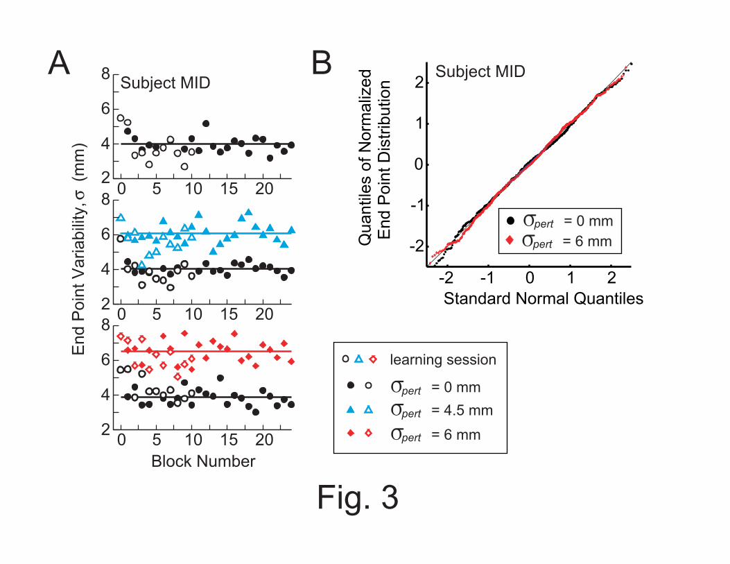
Before we started to collect data for a given perturbation, subjects practiced with

that perturbation for 270 trials with penalties of 0 and 200. In all cases, the variances of

the actual end points for each subject reached a stable value within the first 5 blocks (i.e.,

the first 120 trials) of the learning session (Fig. 3A). We also examined reaction times and

movement times and found that neither differed significantly across conditions (p > 0.05

for each subject in all cases). Reaction and movement times remained constant for the

duration of the experiment. This indicates that the timing of movements was the same

across experimental conditions.

Homogeneity and isotropy of variance across target-penalty configurations and penalty amounts

Movement variability differed significantly across subjects, so we analyzed the data

separately for each subject. In analyzing the data, it is useful to distinguish three

distributions. 1) We refer to the distribution of finger-tip positions when the finger

contacted the surface as PDFfinger (where PDF stands for probability distribution function);

2) The distribution of perturbations of the visual representation of the finger tip is PDFpert.

As stated earlier, the perturbation was added to the actual finger position and was an

6

isotropic Gaussian with mean = 0 and variance = 2pertσ (upon contact). 3) The distribution

of the visual representation of the finger tip when it contacted the surface is PDFvisual. We

found that the variances of finger position (PDFfinger) in the x- and y-directions were

independent of conditions and isotropic (p>0.05 in all cases). In particular, we found no

evidence of a correlation between the x- and y-directions.

Gaussian distribution of movement end points

We asked what the form of PDFfinger was. Fig. 3B compares PDFfinger to a Gaussian

distribution. In constructing the figure, the x- and y-coordinate of each end point were

treated identically, as if they were drawn from the same distribution. For each quantile of

this combined set of x and y end points, Fig. 3B plots a point with ordinate value equal to

the z-score of the corresponding end-point position, and abscissa value equal to the

quantile for a normal distribution with mean = 0 and standard deviation = 1. The close

correspondence between the resulting data points and the solid diagonal line is strong

evidence that the distribution is Gaussian. This was the case for all three amounts of

effective response variance 2pertσ , including zero. Because the distributions of the x- and

y-coordinates of the end points were identical (i.e., isotropic), in the rest of the paper we

compute estimates of observers’ end-point variability by averaging the variance of the x-

and y-coordinates of the end points.

Additivity of motor and visually imposed response variability

We next tested whether subjects compensated for the experimentally imposed

perturbation (PDFpert) by altering finger position during the movement. When asked about

their experience during the experiment, subjects reported that they had noted a decrease

of pointing accuracy and a drop in score (in the conditions in which we added a

perturbation), but were unable to explain the cause of this effect. Consistent with these

reports, two pieces of evidence show that subjects did not compensate for the added

perturbation during movement. First, we examined the variance of PDFfinger for different

amounts of perturbation pertσ . The white bars in Fig. 4 represent 2fingerσ for each value of

pertσ for each subject. 2fingerσ did not vary as a function of pertσ (p>0.05 for all subjects in

7

all cases). (Also, 2fingerσ did not vary with target-penalty configuration, nor with the amount

of the penalty; p>0.05 for all subjects in all cases.) Second, we looked for evidence of

covariation between finger end points and the imposed perturbation. If the two

distributions did not covary, the sum of their variances ( 2 2finger pertσ σ+ ) should equal

2visualσ , the variance of the visually specified end points. The white and black bars in Fig. 4

represent 2fingerσ and 2

pertσ , respectively. Their sum is indeed approximately equal to

2visualσ , which is represented by the red bars (F-test, all p>0.05). Thus, PDFvisual, the

distribution of the effective variance, is well characterized by the sum of two independent

variables with distributions PDFfinger and PDFpert. Furthermore, because PDFpert and

PDFfinger are both Gaussian, PDFvisual must also be Gaussian.

These observations justify our computation of an estimate of the actual end-point

variance 2fingerσ by averaging over the x- and y-directions, all spatial configurations, and

all penalty values.

Optimal compensation for changes in effective movement variance

Because the distribution of movement end points (PDFfinger) was symmetric with

respect to the y-axis, we collapsed the data across the left-right symmetric configurations.

The optimal movement planner (described in detail in the Methods) exhibits a different

horizontal shift of the aim point (and therefore the mean end point) away from the penalty

region for each spatial configuration, penalty level, and amount of perturbation; the

predicted shifts for one subject are represented by the white and orange squares in Fig. 2.

The optimal shift is larger for target positions closer to the penalty region, for higher

penalty values, and for greater perturbations. No predicted shift occurs when the penalty

is zero and when the penalty region is far from the target. The predicted shifts, when they

occur, are always horizontal because the target was displaced horizontally from the

penalty region.

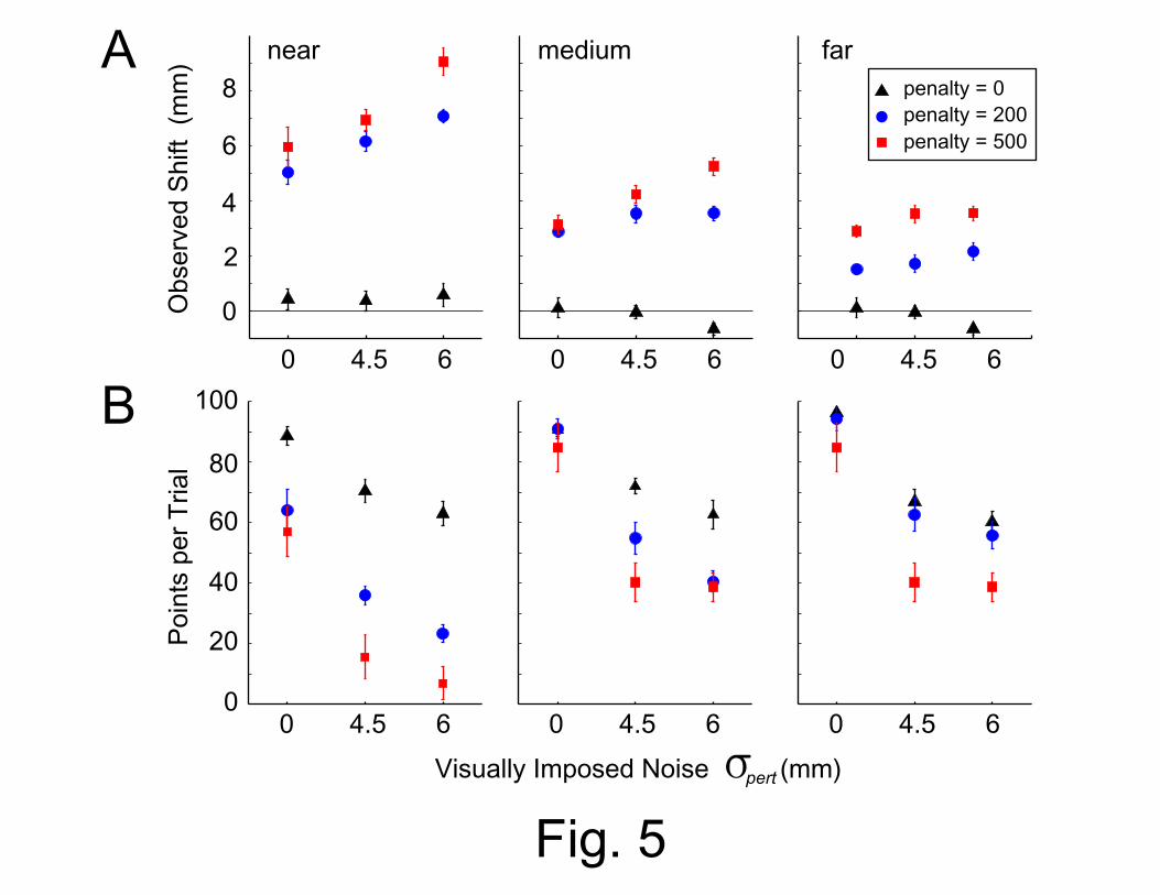
Fig. 5A shows the observed shifts in mean end points (the actual positions of the

finger at the end of the movements) away from the center of the target (averaged over

trials and subjects). We plot only the horizontal component of the shifts because the end

8

points did not shift vertically. Mean movement end points did not shift horizontally in the

zero-penalty condition, nor did they shift when the target and penalty regions were widely

separated. They did shift when the penalty was not zero and the penalty and target were

not widely separated. End points shifted farther from the target center for higher penalties,

closer target positions, and larger perturbations ( pertσ ). In general, the observed shifts are

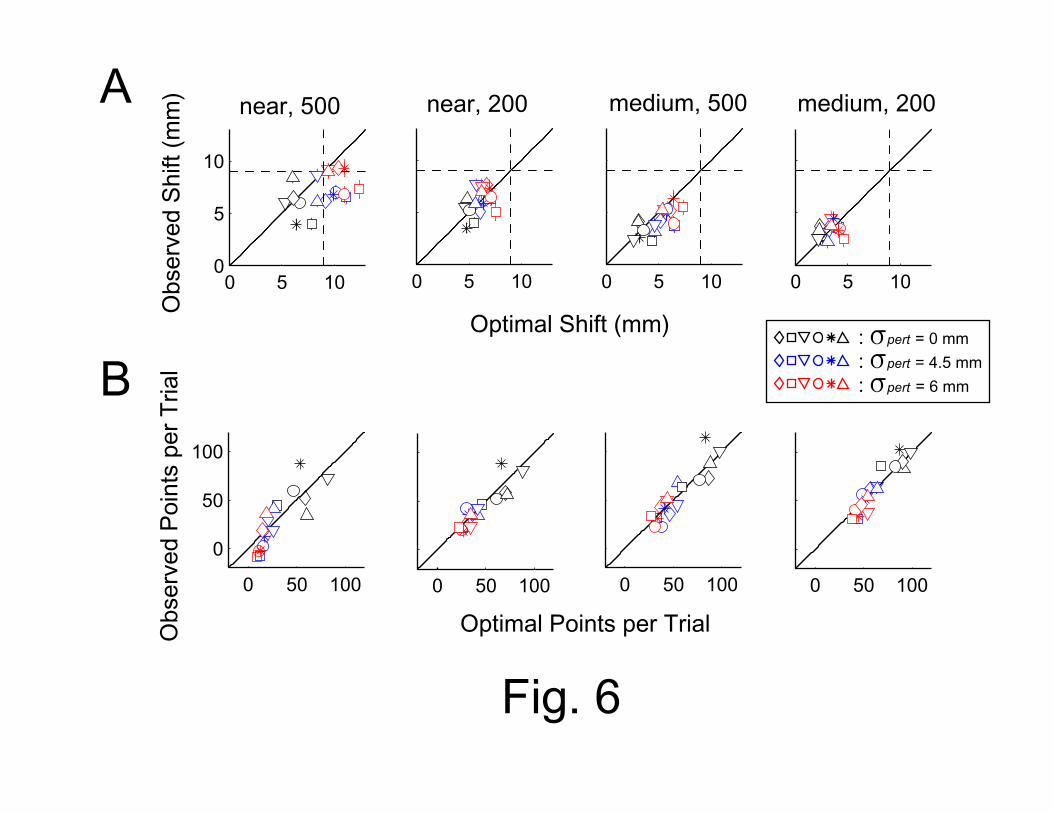
similar to those of the ideal planner. Fig. 6A plots the observed shifts of the actual finger

positions versus the shifts predicted by the optimal planner. The correspondence between

observed and predicted shifts is excellent with one exception: in the near, high-penalty

condition, subjects should have aimed several millimeters outside of the target region

(whose outer edge is represented by the vertical and horizontal dashed lines). Subjects

did shift their end points away from the target center, but not far enough to fall consistently

outside the target region. However, this non-optimal choice of end point had little effect on

the score in the high-variance conditions because the gain landscape in these conditions

is shallow.

Fig. 5B shows the average score per condition averaged across subjects. Scores

were lower with high penalties, closer penalty regions, and larger perturbations ( pertσ ).

These changes in scores are consistent with the behavior of the optimal planner. The

figure plots the observed scores (average points per trial) against the optimal scores. The

correspondence between observed and predicted scores is excellent (see also Table 1)

except for one subject in one condition (CAL, in the highest variance condition). Scores

were otherwise statistically indiscriminable from optimal.

In general, performance did not differ significantly from optimal, indicating that

subjects compensated for visually imposed changes in their effective movement variance

by appropriately adjusting their movement end points.

Discussion

Our results extend the evidence that humans estimate statistical regularities in

motor tasks to improve their performance. For example, Baddeley and colleagues13

examined how movement planners accumulate information across recent trials to

9

compensate for visual displacements of the hand. On a given trial, their subjects pointed

at a target while the visually specified position of the finger tip was shifted by a fixed

amount. On subsequent trials this shift changed according to a random walk plus a noise

component that varied from trial to trial. Baddeley and colleagues varied the balance

between drift rate of the random walk and the magnitude of the independent trial-by-trial

noise. Subjects were nearly 73% efficient relative to an optimal model (a Kalman filter). A

trial-by-trial analysis of those data suggested that subjects gave most weight to errors

from the most recent trials to distinguish shifts due to the random walk from the trial-by-

trial noise. Other studies have shown that subjects also estimate the prior probabilities of

occurrence of different targets in planning movements.14-15

Our results extend this picture. In previously studied tasks, optimal performance

corresponded to separating reliable information from variability (which could then be

ignored). In contrast, optimal performance in our task required an estimate of the

variability. An optimal movement strategy has to take into account not only the

consequences of the intended movement, but also the consequences of unintended ones

(i.e., errors). To achieve that, the optimal strategy is affected by the subject’s effective

movement variability in addition to the stimulus configuration and the relative rewards and

costs associated with the target and penalty regions. Our results demonstrate that the

human movement planning system both takes this movement variability into account and

compensates for changes in variability if these changes interfere with task goals.

Our model is complementary to a recent model of motor coordination based on

stochastic optimal feedback control. Todorov and Jordan9 introduced a “minimal

intervention” principle which assumes that deviations from the average trajectory are

corrected only when they interfere with task performance. Variance is not eliminated, but

rather it is allowed to accumulate in task-irrelevant dimensions. In our experiments, task

relevance is defined explicitly for the subject by the payoffs and penalties associated with

different outcomes. Therefore, optimality requires more than minimizing variability.

Subjects must also reach the target within a specified time-out period; otherwise, they

incur a large penalty. To meet the time constraint, they accept an increase in movement

variability. In our task, minimal intervention means that movement variance should be

reduced as much as possible by using all the time available. Our subjects learned to time

10

their movements such that they hit the screen just before the end of the timeout. As a

result, about 75% of the arrival times fell between 500 ms and the 650 ms time limit, in all

subjects. Subjects hardly ever hit the screen later than 650 ms (less than 10 timeouts per

subject in a total of 2148 trials).

Under different task constraints, subjects will choose a different strategy. They may

endure higher biomechanical costs to improve the stability of their movements. For

example, when moving in the presence of externally applied force fields, subjects maintain

a constant level of movement variance by increasing the stiffness of the arm.16-17 In other

words, every task comes with its own cost function, based on the explicit gains and losses

associated with the possible outcomes of the movement, biomechanical gains, and the

gains associated with the time limits imposed on the mover (Eq. 1). Behavior can only be

classified as optimal or sub-optimal with respect to this pre-specified cost function.

Subjects may deviate from optimality for a variety of reasons. In our experiment,

subjects were generally quite close to optimal with one statistically significant exception

(subject CAL in the large-perturbation condition). It is interesting to note that all subjects

demonstrated a “risk-seeking” behavior in this condition: When the optimal planner

predicted an end point outside the target region, subjects’ mean end points were closer to

the penalty region than predicted (although only two subjects, CAL and SSG, exhibited

efficiencies below 90%; Table 1), as if subjects were reluctant to aim consistently outside

the target region. We conclude that these small deviations from optimality do not indicate

that subjects failed to update the estimate of their own effective movement variance, but

rather that they may have decided to ignore this estimate in some conditions, and aimed

within the target even though aiming outside the target would have yielded a larger gain.

In summary, our subjects compensated for visually imposed increases in variance,

and their performance did not differ significantly from optimal. Our results suggest that

humans take their effective movement variance into account in planning movements and

that they update their estimates of movement variance in response to externally imposed

changes in effective variance.

11

Materials and Methods

Apparatus

The apparatus has been described by Ernst and Banks.18 Visual stimuli were

displayed on a CRT suspended from above. Subjects viewed the stereoscopically

displayed visual stimulus in a mirror using CrystalEyes™ liquid-crystal shutter glasses. A

head-and-chin rest limited head movements. A lightly textured, frontoparallel plane was

presented in front of the subject and the stimuli were presented on this plane. A

PHANToM™ force-feedback device tracked the 3d position of the right index finger. The

hand itself was not visible, but the fingertip was represented visually by a small cursor.

The apparatus was calibrated to assure that the visual and haptic stimuli were

superimposed in the workspace. In some conditions, the visual representation of the

fingertip was displaced from its actual position thereby perturbing the visual feedback (see

Procedure). When the finger reached the visually rendered frontal plane, haptic feedback

was provided by the PHANToM™: the finger “hit” the plane.

Stimuli

The stimuli consisted of a target region and a penalty region (Fig. 1). The target

region was a filled green circle and the penalty region was an unfilled red circle. Overlap

of the target and penalty was readily visible. The target and penalty regions had radii of

9 mm. The target region was displaced left or right from the penalty region by one of three

amounts: near, medium, and far (Fig. 1B).

The position of the penalty region was selected randomly on each trial to prevent

subjects from using pre-planned movements; the position was chosen from a uniform

distribution with a range of ±44 mm relative to screen center. A central 200 × 100-mm

frame indicated the area within which the target and penalty regions could appear.

Procedure

The appearance of a fixation cross indicated the start of the next trial. The subject

moved the right index finger to the starting position, represented by a 24-mm sphere. He

or she was required to stay at the starting position until the stimulus appeared (otherwise,

12

the trial was aborted). The frame was then displayed, followed 500 ms later by the target

and penalty regions. Subjects were required to touch the stimulus plane within 650 ms or

they would incur a timeout penalty of 700 points. The point where the observer touched

the plane is the end point of the movement, denoted ( ),x y . If the subject touched the

plane at a point within the target or penalty region, the region “exploded” visually. The

points awarded for that trial were then shown, followed by the total accumulated points for

that session.

A target hit was always worth 100 points. A penalty hit cost 0, 200, or 500 points,

which was constant during a block of trials. If the stimulus plane was touched in the region

where the target and penalty overlapped, the reward and penalty were both awarded. If a

subject moved from the starting position before or within 100 ms after stimulus

presentation, the trial was abandoned and repeated later during that block.

Visually imposed increase in effective movement variance

At the beginning of each trial, the visually specified position of the fingertip—the

cursor—was in the same 3d location as the fingertip itself. The actual end point where the

finger hit the stimulus plane is ( ),x y . On perturbation trials, the cursor was displaced

smoothly relative to the true, but invisible, location of the fingertip during the second half of

the movement (Fig. 1A; see caption for more details). The displacement on each trial

( ),x y∆ ∆ was chosen from a bivariate Gaussian distribution with mean ( )0,0 and variance

2pertσ ; displacements greater than 12 mm were not presented. The cursor hit the plane at

the visually specified end point ( ),x x y y+ ∆ + ∆ . Rewards and penalties were scored

based on the perturbed (and more variable) visually specified finger position, forcing

subjects to estimate their new effective response variance to optimize performance. Each

subject ran the experiment with three different amounts of perturbation (which in turn

affected the effective response variance): pertσ = 0, 4.5, and 6 mm.

Subjects ran a total of 10 sessions. The first was a practice session during which

the subject learned the timing of the task. In the practice session, subjects first ran 30

trials (five repeats of each of the six spatial configurations) in the zero-penalty condition

13

with no time limit. This was followed by four blocks of 24 trials (i.e., four repeats) with a

moderate time limit of 850 ms, followed by six blocks of 24 trials with a 650-ms time limit.

Then three consecutive sessions were run with each amount of perturbation. The first of

the three sessions was a learning session in which the subject learned the new effective

variance. In the learning session, the subject first ran a warm-up block of 30 trials with

zero penalty. Then the cumulative score was reset to zero and 10 more blocks of 24 trials

were run (five blocks with penalty zero and five with a penalty of 200, penalty level

alternating between blocks). The learning session was followed by two experimental

sessions of 372 trials each. Experimental sessions consisted of 12 warm-up trials followed

by 12 blocks of 30 trials (four blocks for each of the three penalty levels, five repetitions

per target location per block) in random order. Sessions with different amounts of

perturbation were run on different days to facilitate learning of the new effective variance.

The order of exposure to the different amounts of perturbation was counterbalanced

across subjects. Each session lasted about 45 min.

Subjects and instructions

Six subjects participated. Four were unaware of the experimental purpose; the

other two were authors. The four naïve subjects were paid for their participation; they also

received bonus payments determined by their cumulative score (25 cents per

1000 points). All subjects used their right index finger for the pointing movement. Subjects

were told the payoffs and penalties before each block of trials. All subjects but one were

right-handed and all had normal or corrected-to-normal vision. Subjects gave informed

consent before testing.

Model of optimal movement planning

In previous work, we developed a model of optimal movement planning based on

statistical decision theory.11-12 We assume that the goal of movement planning is to select

an optimal visuo-motor movement strategy (i.e., a movement plan) that specifies a desired

movement trajectory, method for using visual feedback control, and so on. In this model,

called MEGaMove (Maximize Expected Gain for Movement planning), the optimal

movement strategy is the one that maximizes expected gain. The model takes into

account explicit gains associated with the possible outcomes of the movement, the

14

mover’s own effective movement variance, biomechanical gains, and gains associated

with the time limits imposed on the mover. Here we summarize the model briefly.

The scene is divided into a number of possibly overlapping regions, iR . For the

conditions of our experiment, the regions associated with non-zero gains are the circular

target and penalty regions. An optimal visuo-motor strategy S on any trial maximizes the

subject’s expected gain

1( ) ( | ) ( | ) ( ),

N

i i timeouti

S G P R S G P timeout S B Sλ=

Γ = + +∑ (1)

where Gi is the gain the subject receives if region Ri is reached on time. P(Ri|S) is the

probability, given a particular choice of strategy S, of reaching region Ri before the time

limit t = timeout has expired,

( | ) ( | )timeouti

iR

P R S P S dτ τ= ∫ , (2)

where timeoutiR is the set of trajectories τ that pass through Ri at some time after the start

of the execution of the visuo-motor strategy and before time t = timeout. The expected

biomechanical costs associated with the selected movement trajectory are represented in

Eq. 1 by a gain function B(S), which is typically negative (a cost or penalty associated with

the trajectory). Because the task involves a penalty for not responding before the time

limit, Eq. 1 contains a term for this timeout penalty. The probability that a visuo-motor

strategy S leads to a timeout is P(timeout | S) and the associated gain is Gtimeout. The

parameter λ characterizes the trade-off the subject will tolerate between physical effort

and expected reward.

In our experiments, subjects win and lose points by touching a stimulus

configuration displayed on a plane. As long as the plane is hit before the timeout,

penalties and rewards depend only on the position of the end point in this plane. In this

effectively two-dimensional task, a strategy S may be identified with the mean end point

on the plane (x,y) that results from adopting strategy S. We assume that the movement

end points ( , )x y′ ′ are Gaussian distributed. Because we found that subjects’ movement

variance was the same in the vertical and horizontal directions,

15

( ) ( ){ }2 2 22

1( , | , ) exp 2 .2

p x y x y x x y y σπσ

⎡ ⎤′ ′ ′ ′= − − + −⎢ ⎥⎣ ⎦ (3)

The probability of hitting region Ri is then,

( | , ) ( , | , ) .i

iR

P R x y p x y x y dx dy′ ′ ′ ′= ∫ (4)

In our experiments, the probability of a timeout and the biomechanical gains are effectively

constant over the limited range of relevant screen locations, so in finding the optimal

solution of Eq. 1, we can ignore the timeout and biomechanical gain terms. Thus, finding

an optimal movement strategy corresponds to choosing a strategy with mean aim point

(x,y) that maximizes,

( )( , ) | ,i ii

x y G P R x y′Γ =∑ . (5)

No analytical solution could be found for maximizing Eq. 5 for our stimulus configurations,

so the integral was solved by integrating Eq. 4 numerically19 and using the results to

maximize Eq. 5.

Data analysis

For each trial, we recorded reaction time (the interval from stimulus display until

movement initiation), movement time (the interval from leaving the start position until the

screen was touched), the movement end position, and the score. Trials in which the

subject left the start position less than 100 ms after stimulus display or hit the screen after

the time limit were excluded from the analysis.

Data format. Each subject contributed approximately 2160 data points; i.e., 80

repetitions per condition (with data collapsed across left-right symmetric configurations).

On each trial, the actual end-point positions ( ) 1,...,80j jx ,y , j = were recorded relative to

the center of the target circle. The corresponding effective end-point positions were

( ),j j j jx x y y+ ∆ + ∆ .

Tests of homogeneity and isotropy of variance of movement end points. For each

amount of perturbation and each subject, we tested whether the variances of the finger

end points ( 2fingerσ ) in the x- and y-directions were affected by manipulations of target

16

location and penalty value. Levene tests20 were performed to test for the homogeneity of

the variances in the x- and y-directions across spatial and penalty conditions and across

amounts of perturbation. We found no significant differences in variance across stimulus

configurations, penalty amounts, and perturbation amounts. We also found that the

distribution of end points (PDFfinger) was isotropic. We computed one estimate of each

subject’s end-point variability ( 2ˆfingerσ ) by averaging variances across spatial and penalty

conditions and across the x- and y-directions.

Test of additivity of variance. From the end-point data, we estimated the subject’s

actual end-point variance 2ˆfingerσ for each level of perturbation ( 2pertσ ). For each 2

pertσ , we

computed 2ˆfingerσ for each of the 18 spatial and penalty conditions in the x- and y-

directions. We then averaged the resulting 36 variance estimates for that 2pertσ . If the

subject’s actual end-point variance is unaffected by the imposed perturbations, 2ˆfingerσ

should be constant across conditions and equal to the expected value 2fingerσ , the

subject’s unperturbed end-point variance. The subject’s effective movement variance 2visualσ was estimated similarly, using ( ),j j j jx x y y+ ∆ + ∆ in place of ( ),j jx y . Effective

movement variance should increase with increasing perturbation 2pertσ and, if the subject’s

actual end-point variance was independent of the amount of perturbation in the visual

representation of the end point, it should be equal to the expected value of 2 2 2visual finger pert=σ σ σ+ . We found this to be the case (Fig. 4).

Responses in symmetric configurations. The target was displaced leftward from the

penalty region in half the trials and rightward in the other half. We asked whether the

movement end points had the same properties in the two types of stimuli, and found that

there were no significant differences. Thus, we averaged data across the leftward and

rightward target displacements for each condition.

Reaction times and movement times. We also looked for changes in reaction and

movement times across conditions. We analyzed both measures for each subject in a 3-

factor, repeated-measures ANOVA. The factors were target position, penalty level, and

17

amount of perturbation. We found no significant differences in reaction or movement time

across these variables.

Effect of spatial and penalty conditions. To determine whether subjects shifted their

movement end points in response to changes in perturbation amount (i.e., effective

movement variance), we analyzed the end points for each subject in a 3-factor, repeated-

measures ANOVA. The factors were target position (averaged over symmetric

configurations), penalty level, and amount of perturbation. The data are displayed in

Figs. 5 and 6.

Comparison to model predictions. Mean movement end points for each condition

were compared with the end points predicted by our model of optimal movement planning.

We calculated the optimal end points (xopt, yopt) based on each subject’s estimated

effective movement variance 2ˆvisualσ for each level of effective response variability

2 2finger pertσ σ+ . Note that yopt = 0 for all conditions. The comparisons are displayed in

Fig. 6.

Efficiency. Each subject’s performance—the total points scored in the experiment—

was compared to optimal performance by computing efficiency. Each subject’s cumulative

score was computed across the conditions of primary interest, which are those in which

the model predicts measurable differences in mean movement end points. These

conditions were the near and medium target-penalty configurations for penalty values of

200 and 500. Efficiency is the subject’s cumulative score divided by the optimal score

predicted by the model. The optimal scores were computed in a Monte Carlo simulation

consisting of 100,000 runs of the optimal movement planner performing the experiment

with each subject’s variance. We calculated the efficiency ratio for each condition and

each subject and expressed the ratio as a percentage. Efficiencies were statistically

indiscriminable from 100% except in one condition with one subject (Table 1).

18

References

1) Bohan, M., Longstaff, M. G., van Gemmert, A. W., Rand, M. K. & Stelmach,

G. E. Effects of target height and width on 2D pointing movement duration and kinematics.

Motor Control 7, 278-289 (2003).

2) Meyer, D. E., Abrams, R. A., Kornblum, S., Wright, C. E. & Smith, J. E.

Optimality in human motor performance: ideal control of rapid aimed movements. Psychol.

Rev. 95, 340-370 (1988).

3) Murata, A. & Iwase, H. Extending Fitts’ law to a three-dimensional pointing task.

Hum. Mov. Sci. 20, 791-805 (2001).

4) Plamondon, R. & Alimi, A. M. Speed/accuracy trade-offs in target-directed

movements. Behav. Brain Sci. 20, 279-349 (1997).

5) Schmidt, R. A., Zelaznik, H., Hawkins, B., Frank, J. S. & Quinn, J. T. Motor

output variance: a theory for the accuracy of rapid motor acts. Psychol. Rev. 86, 415-451

(1979).

6) Smyrnis, N., Evdokimidis, I., Constantinidi, T. S. & Kastrinakis, G. Speed-

accuracy trade-offs in the performance of pointing movements in different directions in

two-dimensional space. Exp. Brain Res. 134, 21-31 (2000).

7) Hamilton, A. F. C. & Wolpert, D. M. Controlling the statistics of action: obstacle

avoidance. J. Neurophysiol. 87, 2434-2440 (2002).

8) Harris, C. M. & Wolpert, D. M. Signal-dependent noise determines motor

planning. Nature 394, 780-784 (1998).

9) Todorov, E. & Jordan, M. I. Optimal feedback control as a theory of motor

coordination. Nat. Neurosci. 5, 1226-1235 (2002).

19

10) Sabes, P. N. & Jordan, M. I. Obstacle avoidance and perturbation sensitivity in

motor planning. J. Neurosci. 17, 7119-7128 (1997).

11) Trommershäuser, J., Maloney, L. T. & Landy, M. S. Statistical decision theory

and the selection of rapid, goal-directed movements. J. Opt. Soc. Am. A 20, 1419-1433

(2003).

12) Trommershäuser, J., Maloney, L. T. & Landy, M. S. Statistical decision theory

and trade-offs in the control of motor response. Spat.Vis. 16, 255-275 (2003).

13) Baddeley, R. J., Ingram, H. A. & Miall, R. C. System identification applied to a

visuomotor task: near-optimal human performance in a noisy changing task. J. Neurosci.

23, 3066-3075 (2003).

14) Körding, K. P. & Wolpert, D. M. Bayesian integration in sensorimotor learning.

Nature 427, 244-247 (2004).

15) Vetter, P. & Wolpert, D. M. Context estimation for sensorimotor control. J.

Neurophysiol. 84, 1026-1034 (2000).

16) Burdet, E., Osu, R., Franklin, D. W., Milner, T. E. & Kawato, M. The central

nervous system stabilizes unstable dynamics by learning optimal impedance. Nature 414, 446-449 (2001).

17) Franklin, D. W., Osu, R., Burdet, E., Kawato, M. & Milner, T. E. Adaptation to

stable and unstable dynamics achieved by combined impedance control and inverse

dynamics model. J. Neurophysiol. 90, 3270-3282 (2003).

18) Ernst, M. O. & Banks, M. S. Human integrate visual and haptic information in a

statistically optimal fashion. Nature 415, 429-433 (2002).

19) Press, W. P., Teukolsky, S. A., Vetterling, W. T. & Flannery, B. P. (eds.)

Numerical Recipes in C. The Art of Scientific Computing 2nd edn. (Cambridge U. Press,

Cambridge, UK, 1992).

20

20) Howell, D. C. Statistical Methods for Psychology 5th edn. (Duxbury, Australia,

2002).

21) Gnanadesikan, R. Methods for Statistical Data Analysis of Multivariate

Observations 2nd edn. (John Wiley & Sons, New York, 1997).

22) Rencher, A. Methods of Multivariate Analysis 2nd edn. (John Wiley & Sons, New

York, 2002).

21

Figure captions

Fig. 1: Experimental stimuli. A) Manipulation of visual feedback. Subjects viewed a

virtual scene on a computer display reflected in a mirror using liquid-crystal shutter

glasses. The scene consisted of a gaze-normal plane and a small sphere (cursor)

representing the unseen fingertip. The green target and red penalty circles appeared on

the plane, and subjects attempted to hit the target, avoiding the penalty, within 650 ms.

The position of the cursor (red line) was perturbed away from the actual trajectory of the

fingertip (blue line) beginning halfway along the trajectory. The direction of the

perturbation was chosen randomly on each trial, but within a trial the direction was fixed

(within a plane parallel to the target plane). The perturbation increased linearly in size until

reaching a value of ( )∆x,∆y as the screen was hit. The perturbation depended on spatial

position of the fingertip and not on the time at which the finger reached a position.

Observers received haptic feedback when they hit the plane. The feedback depended on

the apparent (i.e., the perturbed), rather than the actual, position of the fingertip. Two trials

are shown. In the first, the perturbation drove the cursor away from the penalty and target

(no points scored). In trial 2, with a new target/penalty configuration and new perturbation,

the red cursor landed in the penalty region even though the fingertip did not, resulting in a

penalty of 200 points. B) Stimulus configurations. The green target and red penalty areas

were circular with diameters of 18 mm. The target was displaced leftward or rightward

relative to the penalty region by one of three amounts: near, medium, and far (9, 13.5, and

18 mm, respectively).

Fig. 2: Simulations of an optimal movement planner. 200 simulated responses are

shown per condition for two amounts of perturbation ( pertσ = 0 and 6 mm) and four

combinations of penalty value and target position. Squares indicate the optimal mean end

points. The red and green circles represent the penalty and target regions (centers

indicated by the vertical lines). The two levels of effective movement variability (blue:

visualσ = 3.48 mm, orange: visualσ = 6.19 mm) correspond to subject AAM’s estimated

22

effective variability in the conditions with no perturbation ( pertσ = 0) and the largest

perturbation ( pertσ = 6 mm). The optimal movement planner aims at the center of the

target circle in no-penalty conditions (not shown), but aims farther away from the penalty

circle as penalty value increases, distance to the penalty circle decreases, and pertσ

increases.

Fig. 3: Stability and distribution of effective movement variability. A) Effective

( visualσ ) and actual ( fingerσ ) movement variability (expressed as standard deviations) as a

function of block number. Open symbols indicate learning blocks, and closed symbols

indicate subsequent data collection blocks. In the plots corresponding to conditions with

added noise ( 0pertσ ≠ ), the black symbols indicate fingerσ and the blue and red symbols

indicate visualσ . B) Quantile-quantile plots21-22 of subject MID’s effective movement end

points (PDFvisual). Black corresponds to end points with no movement perturbation

( 0pertσ = ) and red to end points with the largest perturbation ( 6pertσ = mm) (720 data

points per condition; data for no perturbation collected in session 2, 3, and 4, data for

largest perturbation collected in sessions 8, 9, and 10). In each condition, the x and y

values were treated as if they were independent draws from the same distribution. Each

quantile of that distribution is plotted versus the corresponding quantile for a Gaussian

distribution with mean = 0 and standard deviation = 1. The close correspondence of the

data with the diagonal line (indicating the equality of quantiles) is strong evidence that the

end-point distribution is Gaussian.

Fig. 4: Observed end-point variances. A) Effect of varying the perturbation for each

subject. Red bars represent the measured variance 2visualσ of the perturbed cursor

position. The white portion of the other bars represents the measured variance of the

actual finger position 2fingerσ (averaged across the x- and y-directions). The black portion

of those bars represents the variance of the perturbation ( 2pertσ ). The sum of the two

23

variances, 2 2finger pertσ σ+ , is similar to the values of 2

visualσ , indicating that subjects did not

compensate for the added perturbation. Estimates of 2visualσ are an average of 720 data

points per level of perturbation.

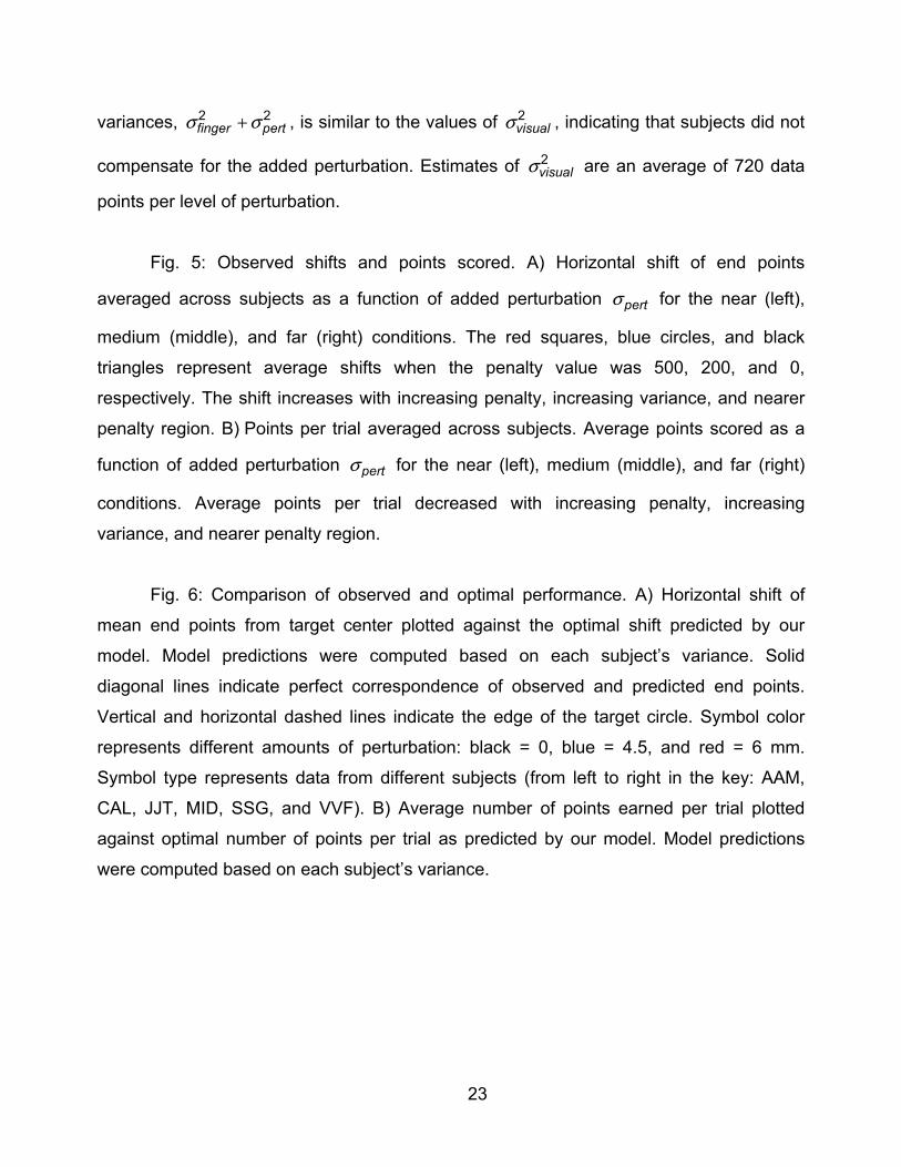
Fig. 5: Observed shifts and points scored. A) Horizontal shift of end points

averaged across subjects as a function of added perturbation pertσ for the near (left),

medium (middle), and far (right) conditions. The red squares, blue circles, and black

triangles represent average shifts when the penalty value was 500, 200, and 0,

respectively. The shift increases with increasing penalty, increasing variance, and nearer

penalty region. B) Points per trial averaged across subjects. Average points scored as a

function of added perturbation pertσ for the near (left), medium (middle), and far (right)

conditions. Average points per trial decreased with increasing penalty, increasing

variance, and nearer penalty region.

Fig. 6: Comparison of observed and optimal performance. A) Horizontal shift of

mean end points from target center plotted against the optimal shift predicted by our

model. Model predictions were computed based on each subject’s variance. Solid

diagonal lines indicate perfect correspondence of observed and predicted end points.

Vertical and horizontal dashed lines indicate the edge of the target circle. Symbol color

represents different amounts of perturbation: black = 0, blue = 4.5, and red = 6 mm.

Symbol type represents data from different subjects (from left to right in the key: AAM,

CAL, JJT, MID, SSG, and VVF). B) Average number of points earned per trial plotted

against optimal number of points per trial as predicted by our model. Model predictions

were computed based on each subject’s variance.

24

Table

Efficiency Subject no noise medium noise high noise

AAM 92.2% 103.5% 102.5%

CAL 107.0% 92.8% 82.4%*

JJT 96.6% 92.2% 93.0%

MID 100.1% 93.2% 93.6%

SSG 114.7% 99.7% 88.8%

VVF 93.8% 109.4% 113.3%

Table 1: Efficiency. Data are reported for the six subjects and three levels of effective

movement variability. Efficiency is the cumulative score in the penalty = 200 and 500

conditions in the near and medium configuration divided by the corresponding expected

score of an optimal movement planner with the same movement variance. Significant

deviations from optimality (outside the 95% confidence interval) are marked by an

asterisk.

∆y∆x

near

medium

far

A B

Fig. 1

18 mm

trial 1

trial 2

-200

near

-200

middle

-500 -500

optimal mean end point, σ = 0 mmoptimal mean end point, σ = 6 mm

σ = 3.48 mmσ = 6.19 mm

Fig. 2

pert

pert

visual

visual

0 10 15 202

4

6

8 Subject MID

0 10 15 202

4

6

8

End

Poi

nt V

aria

bilit

y, σ

(m

m)

0 10 15 20Block Number

2

4

6

8

learning session

σ = 4.5 mmσ = 6 mm

-2 -1 0 1 2

-2

-1

0

1

2

Standard Normal Quantiles

Qua

ntile

s of

Nor

mal

ized Subject MID

End

Poi

nt D

istri

butio

n

5

5

5

A B

Fig. 3

σ = 0 mm

pert

pert

pert

σ = 6 mmpert

σ = 0 mmpert

0

10

20

30

40

50

0

10

20

30

40

50

End

-Poi

nt V

aria

nce

(mm

)2

0 6 0 6 0 4.5 64.5 4.5

Visually Imposed Noise σ (mm)

σσσ

AAM CAL JJT

MID SSG VVF

visually-imposed variability σpert [mm]

Fig. 4

pert

pert

finger

visual

2

2

2

Visually Imposed Noise σ (mm)

Fig. 5

Poi

nts

per

Tria

l O

bser

ved

Shi

ft (

mm

)A

B

0

2

4

6

8

0

20

40

60

80

100

pert

near medium far

4.50 6 4.50 6 4.50 6

4.50 6 4.50 6 4.50 6

penalty = 500penalty = 200penalty = 0

0 50 100

near, 200

0 5 10

0 50 100

0

50

100

near, 500

0 5 100

5

10

0 50 100

medium, 200

0 5 10

Obs

erve

d S

hift

(mm

)

0 50 100

Obs

erve

d P

oint

s pe

r T

rial

medium, 500

0 5 10

Optimal Shift (mm)

Optimal Points per Trial

: σpert = 0 mm

: σpert = 4.5 mm

: σpert = 6 mm

A

B

Fig. 6