Demand analysis (2)

DEMAND ANALYSISUnit 3.1

Prof. Prabha Panth, Osmania University

Demand

• Consumer’s Sovereignty: The consumer influences the market through his demand.

• Demand is the offer to purchase at given prices. • Consumers offer to purchase, because of their

desire for the good/service, backed by ability and willingness to buy.

• The quantity demanded is a flow spread over a different prices, ceteris paribus.

• It can be shown in the form of a d-schedule or a graph.

2 May 2023 2

2 May 2023 3

Demand schedule and D curvePrice (Rs) Q (kgs)

week1 10

2 9

3 8

4 7

5 6

Rs

Q = Kgs0

d

d

P=2

Q=9

a

P=4b

Q=7

Movements on a given d curve, due to change in P called “Changes in Quantity Demanded” or “contraction and expansion of demand.”

2 May 2023 4

The Law of Demand

• Other things remaining constant, the quantity demanded of a commodity is inversely related to its price.

• In other words, if Px then Qx will ↓.• And if Px ↓, then Qx , ceteris paribus.This means consumers are willing to buy

more at lower prices, and less at higher prices.

Factors affecting Q Demanded1. Marginal utility of the commodity (MUx).2. Price of the commodity (Px).3. Price of other related goods: a) Substitutes and

b) Complementary goods.4. Income of the consumer,5. Government policy, taxation,6. Tastes and preferences, 7. Social and religious customs,8. Expectations of future trends in Ps and

incomes.9. Macro economic situation – recession/inflation

2 May 2023 5

2 May 2023 6

Increase and Decrease in Demand

• Q is inversely related to P, other things remaining constant.

• But if other things, such as income, tastes, etc. change, then the total demand curve will shift.

• Increase in Demand means that the entire D-curve shifts upwards to the right, i.e. more is demanded at each price.

• Decrease in Demand means that the entire D-curve shifts downwards to the left, i.e. less is demanded at each price.

2 May 2023 7

Increase in d:

P

0Q

d1

d1

d2

d2

P1

Q1 Q2

a b

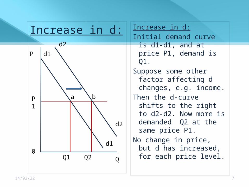
Increase in d:Initial demand curve is d1-

d1, and at price P1, demand is Q1.

Suppose some other factor affecting d changes, e.g. income.

Then the d-curve shifts to the right to d2-d2. Now more is demanded Q2 at the same price P1.

No change in price, but d has increased, for each price level.

2 May 2023 8

Decrease in D:

P

0Q

d2

d2

d1

d1

P1

Q2 Q1

a b

Decrease in D:Initial demand curve is d1-d1,

and at price P1, demand is Q1.

Suppose some other factor affecting d changes, e.g. change in tastes.

Then the d-curve shifts to the left to d2-d2. Now less is demanded Q2 at the same price P1.

No change in price, but d has decreased for each price level

2 May 2023 9

Market Demand

• Sum of individual d-curves at different prices = market demand.

Market D = Σ d-curvesFirms deal with market demand, not

individual demand curves.Have to decide how much will be demanded

by the consumers at different prices.

Market DemandPriceRs

d1 Kgs

d2 kgs

d3 Kgs

D = d1+d2+d3

10 5 8 10 23

9 7 10 14 31

8 10 14 19 43

7 15 20 25 60

6 18 22 28 68

2 May 2023 10

P

0

Q

d1 d2 d3 D

D

P=8 10 14 1943

Q1=43

2 May 2023 11

Significance of Demand to Firms

• Sales forecasting : basis for the sales of firms. • Pricing decisions :Depending on d, the firm can

charge and change the price of its product. • Marketing decisions: Aggressive salesmanship,

advertisements, to boost up demand• Production decisions: how much to produce.• Financial decisions: budgeting and managing the

finances of the firm, depends on the sale revenue earned.

ELASTICITY OF DEMAND

2 May 2023 12

2 May 2023 13

Price Elasticity of Demand

• When P changes, demand normally changes inversely. • But what is the extent of change?

Price Elasticity: measures the responsiveness of Quantity demanded of a commodity, to a change in

its Price, ceteris paribus.• For certain goods, a small change in P can lead to

large change in Qd. (Elastic Demand)• For other goods, a large change in P may lead to a less

than corresponding change in Qd. (Inelastic Demand).

Formula of P-elasticity of D

ep = % change in Q demanded% change in P.

For all normal goods, ep value is negative, showing the inverse relationship between P and Q. Formula is given by:

2 May 2023 14

│ep│= ∆Q/Q = ∆Q . P_∆P/P Q ∆P

2 May 2023 15

Types of Price elasticity1. Zero elasticity: No response

to change in Q demanded, due to change in P. So ep = 0. The D-curve is a vertical straight line.

2. Infinite elasticity: A small fall in P leads to infinite increase in Q demanded.

Here – ep = (infinity). The D-curve is a horizontal straight line.

P

Q0

D

Q1

P0

P1

P

Q0 Q1

P0P1 D

2 May 2023 16

3. Unit elasticity: -ep = 1. Rate of change in Qd is exactly equal to change in price. (∆Q/Q = ∆P/P)

4. Elastic D: – ep>1, Qd responds proportionately more than change in P. Luxury goods. (∆Q/Q > ∆P/P)

5. Inelastic D: – ep < 1, Qd responds proportionately less than change in price. Necessary goods. (∆Q/Q < ∆P/P)

P

Q0 Q1

P0

P1

D

Q0

P

0 Q1

P0

P1

DQ0

P

0 Q1

P0

P1

D

Q0

2 May 2023 17

Slope vs. Elasticity

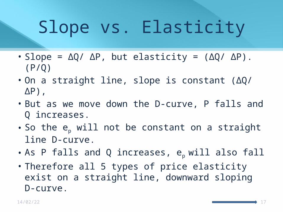
• Slope = ∆Q/ ∆P, but elasticity = (∆Q/ ∆P).(P/Q)• On a straight line, slope is constant (∆Q/ ∆P),• But as we move down the D-curve, P falls and Q

increases. • So the ep will not be constant on a straight line

D-curve.• As P falls and Q increases, ep will also fall• Therefore all 5 types of price elasticity exist on a

straight line, downward sloping D-curve.

2 May 2023 18

Price elasticity on a straight line D-curve

P Q ∆Q/∆P P/Q Ep = (∆Q/∆P).P/Q

10 1

9 2 1/-1 10/1 10

8 3 1/-1 9/2 4.5

7 4 1/-1 8/3 2.66

6 5 1/-1 7/4 1.77

5 6 1/-1 6/5 1.2

4 7 1/-1 5/6 0.83

3 8 1/-1 4/7 0.57

P

0Q

-e>1

-e=1

-e<1

-e=

e=0

Thus ep lies between 0 and - infinity

2 May 2023 19

Total Revenue• Total revenue (TR) = P x Q• if demand is elastic, TR increases as price falls• if demand is inelastic, TR falls as price falls.E.g. P = Rs.5, Qd = 5 Kgs, TR = Rs.5 x 5 kgs = Rs.25, New price P1= Rs.3, Qd = 15 kgs, TR = Rs.3 x 15 kgs = Rs.45,TR increases as P fallsSo, demand for this commodity is elastic

E.g. P = Rs.5, Qd = 5 Kgs, TR = Rs.5 x 5 kgs = Rs.25, New price P1= Rs.3, Qd = 7 kgs, TR = Rs.3 x 7 kgs = Rs.21,TR decreases as P fallsSo, demand for this commodity is inelastic

Price (Rs) Quantity d (Kgs)

TR (P x Q) ep

10 1 109 2 18 e >18 3 24 e >17 4 28 e >16 5 30 e >15 6 30 e =14 7 28 e <13 8 24 e <12 9 18 e <11 10 10 e <1

2 May 2023 20

2 May 2023 21

Factors affecting Price elasticity of D

1. Type of good: Luxuries |e|>1, necessaries |e|<1, extreme necessities, e =0.

2. Number of substitutes: More substitutes -- elastic, less substitutes – inelastic.

3. Time period: Short term, no time to adjust D, so inelastic, Long term – more time to adjust, so more elastic,

4. Size of expenditure on item to total budget: less expenditure, inelastic (e.g. matchbox); more expenditure – elastic (e.g. TV set).

2 May 2023 22

Income elasticity of Demand

• Other things remaining constant, including P of the good, ey is the responsiveness of Qd to a change in the income of the consumer.

ey = ∆Q . Y ∆Y Q

For all normal goods ey > 0, i.e. positive elasticity, when Y increases, Q also increases. Y-d curve is upward sloping.

For inferior goods, ey < 0, i.e. Negative, when Y increases, Qd decreases. Yd curve is downward sloping. Eg. Mud pots, aluminium pots, steel, glass

2 May 2023

Income elasticity of D• Normal Goods:

23

• Inferior Goods:

Y

0 clothes

Y0

Y1

Q0 Q1

a

b

Y

0 Mud pots

Y0

Y1

Q0Q1

a

bYd

Yd

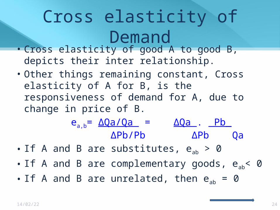
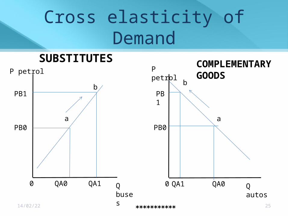
Cross elasticity of Demand• Cross elasticity of good A to good B, depicts their inter

relationship. • Other things remaining constant, Cross elasticity of A

for B, is the responsiveness of demand for A, due to change in price of B.

ea,b= ∆Qa/Qa = ∆Qa . Pb_ ∆Pb/Pb ∆Pb Qa

• If A and B are substitutes, eab > 0• If A and B are complementary goods, eab< 0• If A and B are unrelated, then eab = 0

2 May 2023 24

2 May 2023 25

P petrol

0 Q buses

PB0

PB1

QA0 QA1

a

b

SUBSTITUTESP petrol

0 Q autos

PB0

PB1

QA0QA1

a

b

COMPLEMENTARY GOODS

Cross elasticity of Demand