Decoupling and Recoupling

NBER WORKING PAPER SERIES

DECOUPLING AND RECOUPLING

Anton KorinekAgustín RoitmanCarlos A. Végh

Working Paper 15907http://www.nber.org/papers/w15907

NATIONAL BUREAU OF ECONOMIC RESEARCH1050 Massachusetts Avenue

Cambridge, MA 02138April 2010

We are grateful to Olivier Jeanne and participants at the 2010 AEA meetings for helfpul commentsand to Alejandro Izquierdo (IDB) for kindly providing us with data for emerging countries. A shorterversion of this paper will be published in the American Economic Review Papers and Proceedings(May 2010). The views expressed herein are those of the authors and do not necessarily reflect theviews of the National Bureau of Economic Research.

NBER working papers are circulated for discussion and comment purposes. They have not been peer-reviewed or been subject to the review by the NBER Board of Directors that accompanies officialNBER publications.

© 2010 by Anton Korinek, Agustín Roitman, and Carlos A. Végh. All rights reserved. Short sectionsof text, not to exceed two paragraphs, may be quoted without explicit permission provided that fullcredit, including © notice, is given to the source.

Decoupling and RecouplingAnton Korinek, Agustín Roitman, and Carlos A. VéghNBER Working Paper No. 15907April 2010JEL No. E44,F34,F41

ABSTRACT

We develop a stylized model that captures the phenomena of decoupling and recoupling in an environmentwhere heterogeneous entrepreneurial sectors face financial constraints in their relationship with a commonset of lenders. In response to adverse shocks, a financially constrained sector must reduce its borrowingand cut down on production. In particular, as the constrained sector absorbs less and less capital, thereal interest rate in the economy declines. Other sectors that compete for the same inputs (includingcapital) thus experience lower costs, which boosts investment, output, and profits, reflecting the phenomenonof "decoupling." As long as the shock is small, the entrepreneurial sector repays what is owed andthe lenders' ability to supply funds is unaffected. For large shocks, however, the constrained sectoris no longer able to honor its debts in full and lenders experience losses that erode their lending base.This induces them to cut their supply of credit to the rest of the economy, which reduces output andprofit for all other entrepreneurial sectors, capturing the phenomenon of "recoupling" or contagion.

Anton KorinekUniversity of MarylandTydings Hall 4118FCollege Park, MD [email protected]

Agustín RoitmanDepartment of EconomicsUniversity of MarylandCollege Park, MD [email protected]

Carlos A. VéghDepartment of EconomicsTydings Hall, Office 4118GUniversity of MarylandCollege Park, MD 20742-7211and [email protected]

The financial crisis that has engulfed the world over the past three years

started out in a relatively small set of sectors in a select number of countries,

particularly the real estate sector in the United States. The rise in U.S. in-

terest rates from about 1 to 5 percent between 2004 and 2006 combined with

excessively lax lending standards triggered a wave of defaults on mortgages –

particularly in the sub-prime sector – that led to a slowdown in the housing

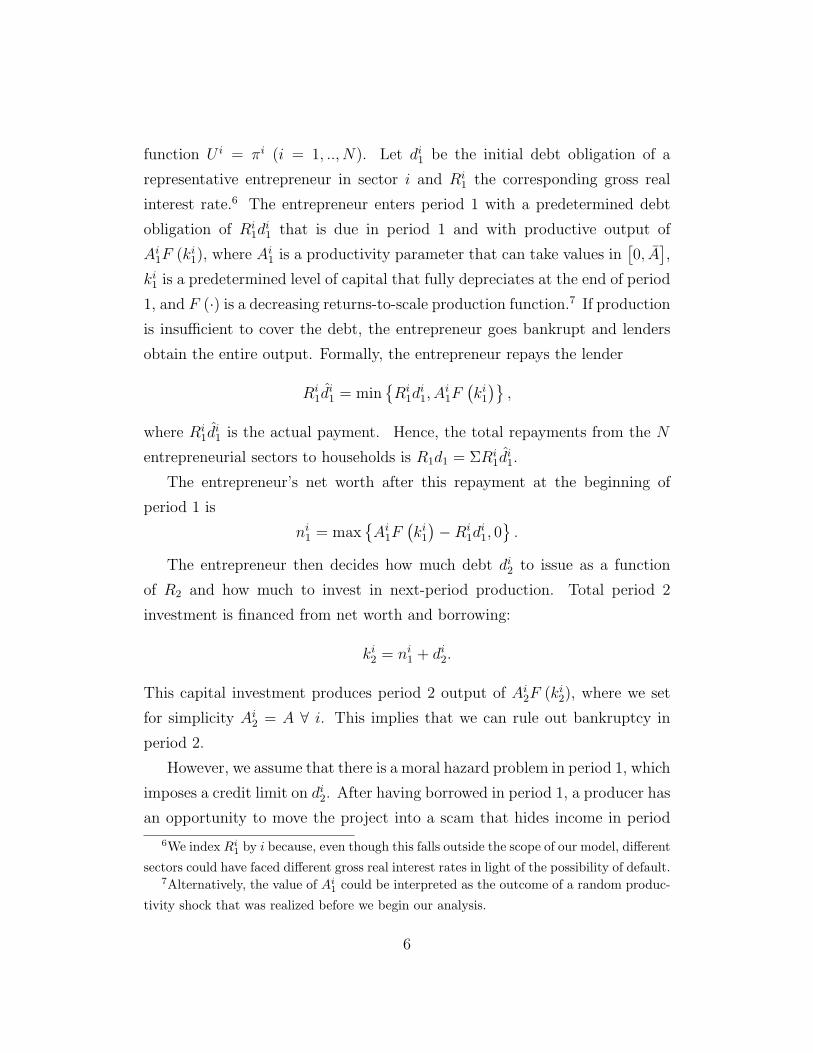
market. As illustrated in Figure 1, Panel A, housing starts peaked in early 2006

and have fallen dramatically ever since. At first (February 2007 to May 2008),

however, financial problems seemed to stay confined to the sectors and coun-

tries in which they originated, with little repercussion on other sectors in the

United States or on emerging countries. Business loans from commercial banks

in the United States, for instance, continued to increase steadily throughout

this period (Panel A). And, if anything, capital inflows into emerging coun-

tries became stronger (Panel B). In fact, policymakers in the developing world

would brag about this “decoupling” from the United States as a sign of the

economic maturity reached by their domestic economies.1 This period of de-

coupling is also evident from looking at corporate bond yields in the United

States (Panel C) and sovereign bond prices for emerging markets (Panel D),

both of which remained relatively unaffected during this period. The decou-

pling, however, began to unravel starting around May 2008 – and particularly

after the collapse of Lehman (September 15, 2008) – as the financial crisis

began to spread like wildfire, affecting countries all around the world, with

asset and stock prices collapsing in unison. In the United States, business

loans plummeted (Panel A) and corporate yields spiked violently (Panel C).

In emerging markets, capital inflows collapsed and bond prices fell dramati-

cally (Panel D).2

1In mid-September 2008, Brazil’s president, Lula da Silva, was quoted as saying “What

crisis? Go ask Bush.” A few weeks later, Brazil’s stock market and currency plummeted

by 20 and 13 percent, respectively (Bloomberg.com, December 3, 2008, “Lula, Like Bush,

Gives Bad Shopping Advice”).2This “decoupling-recoupling” sequence is well documented in Dooley and Hutchinson

(2009) for emerging markets as a whole and in Izquierdo and Talvi (2009) for Latin America.

2

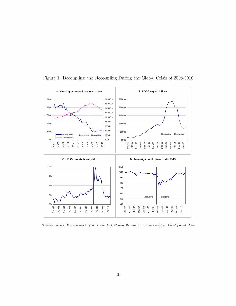
Figure 1: Decoupling and Recoupling During the Global Crisis of 2008-2010

A. Housing starts and business loans

0k

500k

1,000k

1,500k

2,000k

2,500k

Jan-

05

Jul-0

5

Jan-

06

Jul-0

6

Jan-

07

Jul-0

7

Jan-

08

Jul-0

8

Jan-

09

Jul-0

9

Jan-

10

$0bn

$200bn

$400bn

$600bn

$800bn

$1,000bn

$1,200bn

$1,400bn

$1,600bn

$1,800bn

Housing starts

Business loans Decoupling Recoupling

C. US Corporate bond yield

6%

7%

8%

9%

10%

Jan-

05

Jul-0

5

Jan-

06

Jul-0

6

Jan-

07

Jul-0

7

Jan-

08

Jul-0

8

Jan-

09

Jul-0

9

Jan-

10

B. LAC-7 capital inflows

$0bn

$50bn

$100bn

$150bn

$200bn

$250bn

Dec

-02

Jun-

03

Dec

-03

Jun-

04

Dec

-04

Jun-

05

Dec

-05

Jun-

06

Dec

-06

Jun-

07

Dec

-07

Jun-

08

Dec

-08

Jun-

09

Decoupling Recoupling

D. Sovereign bond prices. Latin EMBI

40

50

60

70

80

90

100

110

Jan-

07

Apr

-07

Jul-0

7

Oct

-07

Jan-

08

Apr

-08

Jul-0

8

Oct

-08

Jan-

09

Apr

-09

Jul-0

9

Oct

-09

Jan-

10

Decoupling Recoupling

Sources: Federal Reserve Bank of St. Louis, U.S. Census Bureau, and Inter-American Development Bank

3

This paper develops a stylized model of decoupling and recoupling that cap-

tures these phenomena in an environment where heterogeneous entrepreneurial

sectors face financial constraints in their relationship with a common set of

lenders. In response to adverse shocks, a financially constrained sector must

reduce its borrowing and cut down on production. In particular, as the

constrained sector absorbs less and less capital, the real interest rate in the

economy declines. Other sectors that compete for the same inputs (including

capital) thus experience lower costs, which boosts investment, output, and

profits, reflecting the phenomenon of “decoupling.” As long as the shock is

small, the entrepreneurial sector repays what is owed and the lenders’ ability

to supply funds is unaffected. If the adverse shock exceeds a certain threshold,

however, the constrained sector is no longer able to honor its debts in full and

lenders experience losses that erode their lending base. This induces them to

cut their supply of credit to the rest of the economy, which reduces output

and profit for all other entrepreneurial sectors, capturing the phenomenon of

“recoupling” or contagion.3

1 Model

We assume an economy with one homogenous consumption/investment good

that spans over two time periods t = 1, 2. The economy consists of a combined

household/banking sector that provides finance and values consumption, and

N entrepreneurial sectors that access finance to engage in production and value

final profits.4 We can interpret this set-up alternatively as a world in which

(i) households provide finance to N different countries through global capital

markets or (ii) a closed economy with N different productive sectors.

3For empirical documentation that episodes of contagion typically involve common

lenders, see Kaminsky, Reinhart, and Vegh (2003).4For analytical simplicity, we combine households and banks in our model. As discussed

below, our results would be magnified if we separated the two sectors and allowed for leverage

in the banking sector.

4

1.1 Household/Banking Sector

The consolidated household/banking sector consists of a continuum of identical

agents that have an exogenous and constant endowment e per period and con-

sume ct, which provides utility according to the function U = log (c1)+log (c2).

A representative household obtains repayments R1d1 from the entrepreneurial

sectors at the beginning of period 1, where d1 is the total amount owed by

the entrepreneurs and R1 is an average gross real interest rate. The household

also provides d2 in loans to the entrepreneurial sectors at a gross real interest

rate of R2 to be repaid in period 2. We assume that d1 > 0 to ensure that

households have an incentive to lend, i.e. d2 > 0. The optimization problem

of households/banks is

maxd2

log (e+R1d1 − d2) + log (e+R2d2) , (1)

leading to the first-order condition

R2 =c2c1.

It is easy to show that c1 is a decreasing function of R2.5 Since

d2 = e+R1d1 − c1, (2)

this implies that d2, the supply of loans to entrepreneurs in period 1, is in-

creasing in R2. Further, a reduction in d1 will shift leftward the supply of

loans for a given R2.

1.2 Entrepreneurial Sector

We assume that each of the N entrepreneurial sectors consists of a continuum

of identical entrepreneurs of mass 1 that are risk-neutral and value their profits

πi, which they consume at the end of period 2, according to the linear utility

5As shown in the appendix, this result holds for more general utility functions under

certain regularity conditions.

5

function U i = πi (i = 1, .., N). Let di1 be the initial debt obligation of a

representative entrepreneur in sector i and Ri1 the corresponding gross real

interest rate.6 The entrepreneur enters period 1 with a predetermined debt

obligation of Ri1di1 that is due in period 1 and with productive output of

Ai1F (ki1), where Ai1 is a productivity parameter that can take values in[0, A

],

ki1 is a predetermined level of capital that fully depreciates at the end of period

1, and F (·) is a decreasing returns-to-scale production function.7 If production

is insufficient to cover the debt, the entrepreneur goes bankrupt and lenders

obtain the entire output. Formally, the entrepreneur repays the lender

Ri1di1 = min

{Ri

1di1, A

i1F

(ki1

)},

where Ri1di1 is the actual payment. Hence, the total repayments from the N

entrepreneurial sectors to households is R1d1 = ΣRi1di1.

The entrepreneur’s net worth after this repayment at the beginning of

period 1 is

ni1 = max{Ai1F

(ki1

)−Ri

1di1, 0

}.

The entrepreneur then decides how much debt di2 to issue as a function

of R2 and how much to invest in next-period production. Total period 2

investment is financed from net worth and borrowing:

ki2 = ni1 + di2.

This capital investment produces period 2 output of Ai2F (ki2), where we set

for simplicity Ai2 = A ∀ i. This implies that we can rule out bankruptcy in

period 2.

However, we assume that there is a moral hazard problem in period 1, which

imposes a credit limit on di2. After having borrowed in period 1, a producer has

an opportunity to move the project into a scam that hides income in period

6We index Ri1 by i because, even though this falls outside the scope of our model, different

sectors could have faced different gross real interest rates in light of the possibility of default.7Alternatively, the value of Ai

1 could be interpreted as the outcome of a random produc-

tivity shock that was realized before we begin our analysis.

6

2. Creditors can challenge this in court but can recover at most a fraction

[α/(1 + α)] ∈ (0, 1) of the entrepreneur’s total assets because of imperfect

enforcement. To avoid losses from potential fraud, creditors limit the amount

of borrowing by entrepreneurs to

di2 ≤α

1 + αki2 or di2 ≤ αni1.

The optimization problem of a representative entrepreneur in sector i con-

sists of choosing di2 to maximize profits subject to the borrowing constraint

and is described by the Lagrangian:

Li = AF(ni1 + di2

)−R2d

i2 − λi

(di2 − αni1

),

where λi is the shadow price on the borrowing constraint. The problem results

in the first-order condition

AF ′(ki2

)= R2 + λi.

If the constraint is loose, this reduces to the standard neoclassical condition.

Entrepreneurs invest and borrow optimally:

k∗2 (R2) = F ′−1 (R2/A) ,

di2 = k∗2 (R2)− ni1. (3)

The optimal capital stock is independent of individual-specific variables and

only depends on the cost of capital R2 in the economy. This yields period 2

profits of

πiunc = AF (k∗2 (R2))−R2

[k∗2 (R2)− ni1

],

where it is straightforward to show that ∂πi/∂ni1 > 0 and ∂πi/∂R2 < 0 as long

as the entrepreneur is a net borrower, i.e. ni1 < k∗2 (R2).

If the constraint is binding, a wedge opens between the entrepreneur’s cost

of funds and the marginal product, in which case the level of borrowing and

investment are determined by the constraints

di2 = αni1,

ki2 = (1 + α)ni1.

7

The capital stock is now independent of the real interest rate in the economy

and only depends on entrepreneurial net worth. This results in period 2 profits

given by

πicon = AF((1 + α)ni1

)− αR2n

i1,

which also satisfies ∂πi/∂ni1 > 0 and ∂πi/∂R2 < 0.

Note that if ni1 = 0 because of bankruptcy in period 1, the entrepreneur

cannot borrow and invest due to the constraint, and thus produces and con-

sumes zero in period 2.

2 Equilibrium

For given initial conditions, a decentralized equilibrium in the economy consists

of a bundle {(di2, ki2, R2)}Ni=1 that is a solution to the maximization problems of

the household/banking and the entrepreneurial sectors and satisfies the market

clearing condition for debt

d2 = Σdi2.

Our characterization of the economy’s equilibrium allows us to study the

phenomena of decoupling and recoupling. For simplicity, we assume there are

two productive sectors labeled by i = X,Z, of which sector Z has a value of AZ1

that is sufficiently high so as to be always unconstrained during the ensuing

experiment. We study how the equilibrium changes as we vary the productivity

of sector X over the range[0, A

]for given initial capital and debt positions. To

capture the traditional role of entrepreneurs as net demanders of finance, we

assume that the initial debt and capital levels of both entrepreneurial sectors

are such that they remain net borrowers in period 1.

2.1 Unconstrained Economy

If period 1 productivity in sector X is sufficiently high AX1 ≥ AXunc, the sector

is unconstrained and the economy follows standard neoclassical rules. The

8

threshold AXunc is determined by the productivity level AX1 that leads to a

sectoral net worth nX1 such that

(1 + α)nX1 = k∗2.

Households receive the promised amount R1d1 = RX1 d

X1 + RZ

1 dZ1 in period 1

and supply loans according to (2), and both entrepreneurial sectors demand

loans according to their optimality condition (3).

Within this region, greater sectorX productivity means higher entrepreneurial

net worth nX1 and therefore a lower demand for loans dX2 (R2). As a result, the

interest rate R2 declines, and the optimum amount of investment as well as

profits in both sectors increase. A positive shock in sector X therefore spills

over positively to sector Z.

2.2 Decoupling

If the productivity of sector X drops below AXunc, the sector becomes con-

strained. As long as net worth nX1 is positive, the sector can honor its repay-

ments and households receive the promised amount R1d1 in period 1. This is

the case as long as

AX1 ≥ RX1 d

X1 /F

(kX1

)≡ AXfail.

Within this region, lower period 1 productivity for a constrained entrepreneur

tightens the constraint, leads to lower loan demand and a lower interest rate

R2. Sector Z reacts by increasing investment and profits, i.e., a negative shock

in sector X spills over positively to sector Z. The worse the productivity shock

for sector X, the better off is sector Z – there is decoupling.8

8Note that there are two effects on the welfare of sector X: on the one hand, it is hurt

by the binding constraint, but on the other hand it benefits from the lower interest rate.

The net effect of the two can initially be positive. However, as productivity declines further

and the sector approaches the bankruptcy threshold, sectoral welfare will unambiguously

decline until it reaches zero at the threshold.

9

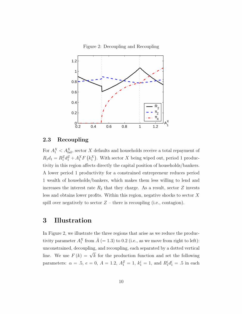
Figure 2: Decoupling and Recoupling

0.2 0.4 0.6 0.8 1 1.20

0.2

0.4

0.6

0.8

1

1.2

A1X

R2

πZ

πX

2.3 Recoupling

For AX1 < AXfail, sector X defaults and households receive a total repayment of

R1d1 = RZ1 d

Z1 +AX1 F

(kX1

). With sector X being wiped out, period 1 produc-

tivity in this region affects directly the capital position of households/bankers.

A lower period 1 productivity for a constrained entrepreneur reduces period

1 wealth of households/bankers, which makes them less willing to lend and

increases the interest rate R2 that they charge. As a result, sector Z invests

less and obtains lower profits. Within this region, negative shocks to sector X

spill over negatively to sector Z – there is recoupling (i.e., contagion).

3 Illustration

In Figure 2, we illustrate the three regions that arise as we reduce the produc-

tivity parameter AX1 from A (= 1.3) to 0.2 (i.e., as we move from right to left):

unconstrained, decoupling, and recoupling, each separated by a dotted vertical

line. We use F (k) =√k for the production function and set the following

parameters: α = .5, e = 0, A = 1.2, AZ1 = 1, ki1 = 1, and Ri1di1 = .5 in each

10

sector i.

For high values of the productivity parameter AX1 , i.e., to the right of

the figure, both sectors are unconstrained and lower productivity in sector X

decreases profits (i.e., welfare) in both sectors as the cost of capital increases.

In the center of the figure, there is decoupling: since the demand for loans

of sector X is progressively constrained, the interest rate declines and sector

Z is better off. In the left region of the figure, sector X goes bankrupt and

the supply of loans to the entrepreneurial sector is reduced, pushing up the

interest rate R2.9 This hurts sector Z, i.e., there is recoupling.

4 Extensions

There are several dimensions in which our benchmark model can be extended

to provide further insights:

(i) Dynamics In the recent financial crisis, decoupling and recoupling oc-

curred sequentially, whereas in our model we are, strictly speaking, con-

ducting a comparative statics exercise. In a multi-period version of our

model, recoupling could occur after an episode of decoupling, if a series

of adverse shocks progressively depletes the net worth of a constrained

sector to the point where it is pushed into bankruptcy.

(ii) Factor Prices In our benchmark model, the only factor of production

is capital. More generally, other factors, such as labor or commodities,

are complements to capital in standard production functions. The less

capital is employed in the economy, the lower is the demand for other

factors. This would lead to a fall in commodity prices and, in labor

markets with sticky wages, to unemployment.

9Note that this channel of transmission is consistent with the evidence presented in Figure

1, where we can see that business loans begin to fall (Panel A) and corporate yield rates

spike sharply (Panel C) at the begining of the recoupling period.

11

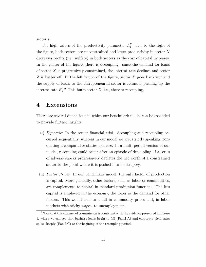
Figure 3: Recoupling with Bankruptcy Costs

0.2 0.4 0.6 0.8 1 1.20

0.2

0.4

0.6

0.8

1

1.2

A1X

R2

πZ

πX

(iii) Bankruptcy Costs If we add to our model bankruptcy costs that reduce

the recovery rate on assets seized by banks by a factor δ in case of

bankruptcy, then there is a discontinuity at Afail that would cause the

interest rate to jump up and welfare to fall, magnifying the impact of

defaults. An example of this is given in Figure 3.

(iv) Leveraged Banks Modifying our benchmark model by separating house-

holds and the banking sector and introducing leverage in the latter can

amplify the propagation of defaults. Leverage implies that the impact

of a shock on the net worth of banks is magnified. Hence, if banks ex-

perienced financial constraints in their relationship with households, our

contagion results would be strengthened.

(v) Efficiency Considerations In the framework we have described in this

paper, the decentralized equilibrium is constrained-efficient, since there

are no actions that a planner could undertake to coordinate the economy

on a better equilibrium. However, if we introduce additional degrees of

freedom for our agents, such as the possibility to choose the amount

of initial debt, inefficiencies may arise. This is particularly the case if

12

there are relative prices, such as exchange rates or asset prices, that are

adversely affected by contagion dynamics (see e.g. Korinek, 2010).

We explore these extensions in more detail in our companion paper (Ko-

rinek, Roitman and Vegh, 2010).

5 Conclusions

We have presented a stylized model that captures the decoupling-recoupling

phenomenon observed after the subprime crisis erupted in the United States

in February 2007 There are two “sectors” in our model that experience first

decoupling and then recoupling as productivity falls in one of them. These

two sectors could be given a literal interpretation (i.e., the real estate and

manufacturing sectors within a country being financed by the financial sector)

or a broader interpretation in terms of different countries (i.e., United States

and Brazil being financed by international capital markets). In our companion

paper, we embed this mechanism in a model with leverage and show how this

decoupling-recoupling cycle is further amplified.

References

[1] Dooley, Michael P., and Michael M. Hutchison. 2009. “Transmission of the

U.S. Subprime Crisis to Emerging Markets: Evidence on the Decoupling-

Recoupling Hypothesis,“ NBER Working Paper No. 15120.

[2] Izquierdo, Alejandro, and Ernesto Talvi. 2009. Policy Trade-offs for Un-

precedented Times. Washington, DC: IDB.

[3] Kaminsky, Graciela L., Carmen M. Reinhart and Carlos A. Vegh. 2003.

“The Unholy Trinity Of Financial Contagion.” Journal of Economic Per-

spectives 17(4): 51-74.

13

[4] Korinek, Anton. 2010. “Regulating Capital Flows to Emerging Markets:

An Externality View.” Unpublished.

[5] Korinek, Anton, Agustın Roitman, and Carlos A. Vegh. 2010. “A Dynamic

Model of Decoupling and Recoupling.” Unpublished.

6 Mathematical Appendix

6.1 Household/Banking Sector

For general utility functions, the first order condition to the optimization prob-

lem of the household/banking sector (1) is

u′ (c1) = R2u′ (c2) .

By implicitly differentiating this Euler equation, we obtain the slope of the

supply of lendingdd2

dR2

= −u′ (c2) +R2d2u

′′ (c2)

u′′ (c1) +R2u′′ (c2).

Since the denominator is negative, this expression is unambiguously positive

as long as the following condition is met:

Condition 1 ∂R2u′(c2)∂R2

= u′ (c2) +R2d2u′′ (c2) > 0

Intuitively, the condition states that the consumer’s marginal period 2 util-

ity from lending in period 1 responds positively to higher interest rates – the

effect consists of the (positive) marginal utility u′ (c2) gained from the higher

interest rate minus the (negative) indirect effect that the marginal utility de-

clines at rate u′′ (c2) as consumption rises.

There are two alternative sufficient conditions under which the condition is

satisfied. First, it is met whenever the curvature of the households utility func-

tion as measured by the coefficient of risk aversion u′′ (·) /u′ (·) is sufficiently

14

low so that increases in consumption do not depress the marginal utility at too

fast of a rate. This is for example the case for log-utility as in our specification

of the household’s problem in (1). For that case we find that

u′ (c2) +R2d2u′′ (c2) =

1

c2

[1− R2d2

c2

]> 0,

since the payment obtained R2d2 < e + R2d2 = c2 and the fraction is always

less than one.

Secondly, the condition is met for arbitrary utility functions whenever the

amount lent d2 is sufficiently low. For example, for the class of CRRA utility

functions with a coefficient of relative risk aversion θ, we find

u′ (c2) +R2d2u′′ (c2) = c−θ2

[1− θR2d2

c2

].

As long as d2 is sufficiently low so that θR2d2 < c2, the condition is satisfied.

For the standard value θ = 2 that is often chosen in the literature, the repay-

ment received has to constitute less than half of total consumption. This is

generally satisfied in models where households derive approximately two thirds

of their income from labor.

The response of the period 2 lending rate R2 to changes in the period 1

repayment isdR2

d (R1d1)=

u′′ (c1)

u′ (c2) +R2d2u′′ (c2).

This derivative is negative whenever condition 1 is met, as is the case for the

log-utility that we used in problem (1).

15