Data Hiding

1Data Mining

Vipin KumarUniversity of Minnesota

Pang-Ning TanMichigan State University

Michael SteinbachUniversity of Minnesota

1.1 Introduction . . . . . . . . . . . . . . . . . . . . . . . . . . . . . . . . . . . . . . . . . . . . 1-1Data Mining Tasks and Techniques • Challenges ofData Mining • Data Mining and the Role of DataStructures and Algorithms

1.2 Classification . . . . . . . . . . . . . . . . . . . . . . . . . . . . . . . . . . . . . . . . . . . 1-6Nearest-neighbor classifiers • Proximity Graphs forEnhancing Nearest Neighbor Classifiers

1.3 Association Analysis . . . . . . . . . . . . . . . . . . . . . . . . . . . . . . . . . . 1-8Hash Tree Structure • FP-Tree Structure

1.4 Clustering . . . . . . . . . . . . . . . . . . . . . . . . . . . . . . . . . . . . . . . . . . . . . . 1-15Hierarchical and Partitional Clustering • NearestNeighbor Search and Multi-dimensional AccessMethods

1.5 Conclusion . . . . . . . . . . . . . . . . . . . . . . . . . . . . . . . . . . . . . . . . . . . . . 1-19

1.1 Introduction

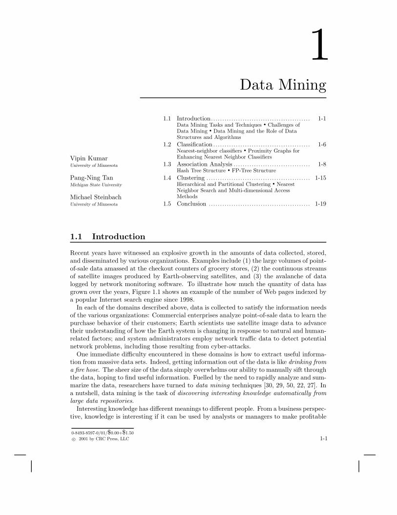
Recent years have witnessed an explosive growth in the amounts of data collected, stored,and disseminated by various organizations. Examples include (1) the large volumes of point-of-sale data amassed at the checkout counters of grocery stores, (2) the continuous streamsof satellite images produced by Earth-observing satellites, and (3) the avalanche of datalogged by network monitoring software. To illustrate how much the quantity of data hasgrown over the years, Figure 1.1 shows an example of the number of Web pages indexed bya popular Internet search engine since 1998.

In each of the domains described above, data is collected to satisfy the information needsof the various organizations: Commercial enterprises analyze point-of-sale data to learn thepurchase behavior of their customers; Earth scientists use satellite image data to advancetheir understanding of how the Earth system is changing in response to natural and human-related factors; and system administrators employ network traffic data to detect potentialnetwork problems, including those resulting from cyber-attacks.

One immediate difficulty encountered in these domains is how to extract useful informa-tion from massive data sets. Indeed, getting information out of the data is like drinking froma fire hose. The sheer size of the data simply overwhelms our ability to manually sift throughthe data, hoping to find useful information. Fuelled by the need to rapidly analyze and sum-marize the data, researchers have turned to data mining techniques [30, 29, 50, 22, 27]. Ina nutshell, data mining is the task of discovering interesting knowledge automatically fromlarge data repositories.

Interesting knowledge has different meanings to different people. From a business perspec-tive, knowledge is interesting if it can be used by analysts or managers to make profitable

0-8493-8597-0/01/$0.00+$1.50

c© 2001 by CRC Press, LLC 1-1

1-2

11/11/1998 8/15/2000 3/1/2001 11/25/2001 1/24/2002 2/3/20030

0.5

1

1.5

2

2.5

3

3.5x 10

9 Number of Web pages indexed by Google Search Engine

FIGURE 1.1: Number of Web pages indexed by the Google c© search engine (Source: In-ternet Archive, http:www.archive.org).

business decisions. For Earth Scientists, knowledge is interesting if it reveals previouslyunknown information about the characteristics of the Earth system. For system adminis-trators, knowledge is interesting if it indicates unauthorized or illegitimate use of systemresources.

Data mining is often considered to be an integral part of another process, called Knowl-edge Discovery in Databases (or KDD). KDD refers to the overall process of turning rawdata into interesting knowledge and consists of a series of transformation steps, includingdata preprocessing, data mining, and postprocessing. The objective of data preprocessingis to convert data into the right format for subsequent analysis by selecting the appropriatedata segments and extracting attributes that are relevant to the data mining task (fea-ture selection and construction). For many practical applications, more than half of theknowledge discovery efforts are devoted to data preprocessing. Postprocessing includes alladditional operations performed to make the data mining results more accessible and easierto interpret. For example, the results can be sorted or filtered according to various measuresto remove uninteresting patterns. In addition, visualization techniques can be applied tohelp analysts explore data mining results.

1.1.1 Data Mining Tasks and Techniques

Data mining tasks are often divided into two major categories:

Predictive The goal of predictive tasks is to use the values of some variables topredict the values of other variables. For example, in Web mining, e-tailers areinterested in predicting which online users will make a purchase at their Website. Other examples include biologists, who would like to predict the functionsof proteins, and stock market analysts, who would like to forecast the future

Data Mining 1-3

prices of various stocks.

Descriptive The goal of descriptive tasks is to find human-interpretable patterns thatdescribe the underlying relationships in the data. For example, Earth Scientistsare interested in discovering the primary forcings influencing observed climatepatterns. In network intrusion detection, analysts want to know the kinds ofcyber-attacks being launched against their networks. In document analysis, it isuseful to find groups of documents, where the documents in each group share acommon topic.

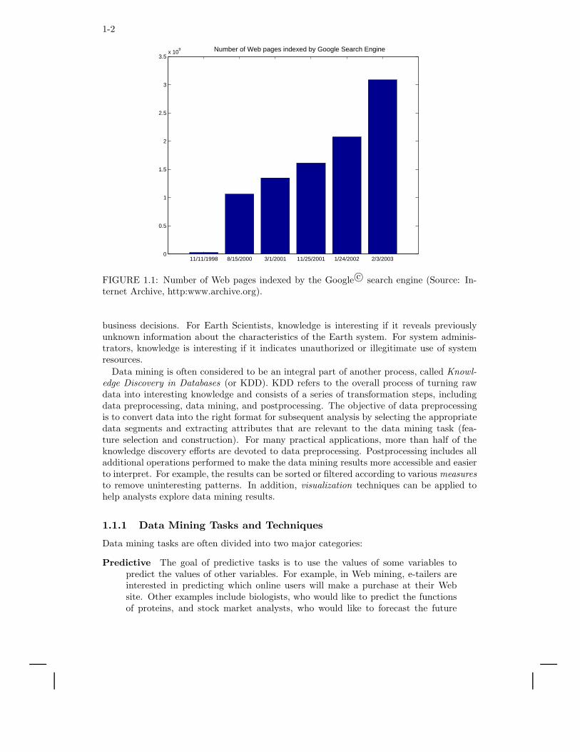
Data mining tasks can be accomplished using a variety of data mining techniques, asshown in Figure 1.2.

Tid Refund Marital Status

Taxable Income Cheat

1 Yes Single 125K No

2 No Married 100K No

3 No Single 70K No

4 Yes Married 120K No

5 No Divorced 95K Yes

6 No Married 60K No

7 Yes Divorced 220K No

8 No Single 85K Yes

9 No Married 75K No

10 No Singl e 90K Yes

11 No Married 60K No

12 Yes Divorced 220K No

13 No Single 85K Yes

14 No Married 75K No

15 No Single 90K Yes 10

Data

Clustering Predict

ive

Modeling

Anomaly

Detection Ass

ociatio

n

Rule Mining

Milk

FIGURE 1.2: Data mining techniques.

• Predictive modelling is used primarily for predictive data mining tasks. Theinput data for predictive modelling consists of two distinct types of variables:(1) explanatory variables, which define the essential properties of the data, and(2) one or more target variables, whose values are to be predicted. For the Webmining example given in the previous section, the input variables correspondto the demographic features of online users, such as age, gender, and salary,along with their browsing activities, e.g., what pages are accessed and for how

1-4

long. There is one binary target variable, Buy, which has values, Yes or No,indicating, respectively, whether the user will buy anything from the Web site ornot. Predictive modelling techniques can be further divided into two categories:classification and regression. Classification techniques are used to predict thevalues of discrete target variables, such as the Buy variable for online users at aWeb site. For example, they can be used to predict whether a customer will mostlikely be lost to a competitor, i.e., customer churn or attrition, and to determinethe category of a star or galaxy for sky survey cataloging. Regression techniquesare used to predict the values of continuous target variables, e.g., they can beapplied to forecast the future price of a stock.

• Association rule mining seeks to produce a set of dependence rules that predictthe occurrence of a variable given the occurrences of other variables. For example,association analysis can be used to identify products that are often purchasedtogether by sufficiently many customers, a task that is also known as marketbasket analysis. Furthermore, given a database that records a sequence of events,e.g., a sequence of successive purchases by customers, an important task is that offinding dependence rules that capture the temporal connections of events. Thistask is known as sequential pattern analysis.

• Cluster analysis finds groupings of data points so that data points that belongto one cluster are more similar to each other than to data points belonging to adifferent cluster, e.g., clustering can be used to perform market segmentation ofcustomers, document categorization, or land segmentation according to vegeta-tion cover. While cluster analysis is often used to better understand or describethe data, it is also useful for summarizing a large data set. In this case, the objectsbelonging to a single cluster are replaced by a single representative object, andfurther data analysis is then performed using this reduced set of representativeobjects.

• Anomaly detection identifies data points that are significantly different thanthe rest of the points in the data set. Thus, anomaly detection techniques havebeen used to detect network intrusions and to predict fraudulent credit cardtransactions. Some approaches to anomaly detection are statistically based, whileother are based on distance or graph-theoretic notions.

1.1.2 Challenges of Data Mining

There are several important challenges in applying data mining techniques to large datasets:

Scalability Scalable techniques are needed to handle the massive size of some ofthe datasets that are now being created. As an example, such datasets typicallyrequire the use of efficient methods for storing, indexing, and retrieving data fromsecondary or even tertiary storage systems. Furthermore, parallel or distributedcomputing approaches are often necessary if the desired data mining task is to beperformed in a timely manner. While such techniques can dramatically increasethe size of the datasets that can be handled, they often require the design of newalgorithms and data structures.

Dimensionality In some application domains, the number of dimensions (or at-tributes of a record) can be very large, which makes the data difficult to an-alyze because of the ‘curse of dimensionality’ [9]. For example, in bioinformatics,

Data Mining 1-5

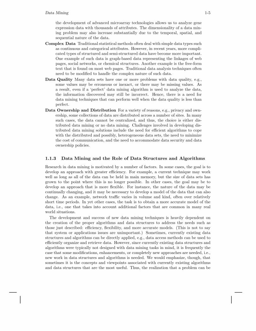
the development of advanced microarray technologies allows us to analyze geneexpression data with thousands of attributes. The dimensionality of a data min-ing problem may also increase substantially due to the temporal, spatial, andsequential nature of the data.

Complex Data Traditional statistical methods often deal with simple data types suchas continuous and categorical attributes. However, in recent years, more compli-cated types of structured and semi-structured data have become more important.One example of such data is graph-based data representing the linkages of webpages, social networks, or chemical structures. Another example is the free-formtext that is found on most web pages. Traditional data analysis techniques oftenneed to be modified to handle the complex nature of such data.

Data Quality Many data sets have one or more problems with data quality, e.g.,some values may be erroneous or inexact, or there may be missing values. Asa result, even if a ‘perfect’ data mining algorithm is used to analyze the data,the information discovered may still be incorrect. Hence, there is a need fordata mining techniques that can perform well when the data quality is less thanperfect.

Data Ownership and Distribution For a variety of reasons, e.g., privacy and own-ership, some collections of data are distributed across a number of sites. In manysuch cases, the data cannot be centralized, and thus, the choice is either dis-tributed data mining or no data mining. Challenges involved in developing dis-tributed data mining solutions include the need for efficient algorithms to copewith the distributed and possibly, heterogeneous data sets, the need to minimizethe cost of communication, and the need to accommodate data security and dataownership policies.

1.1.3 Data Mining and the Role of Data Structures and Algorithms

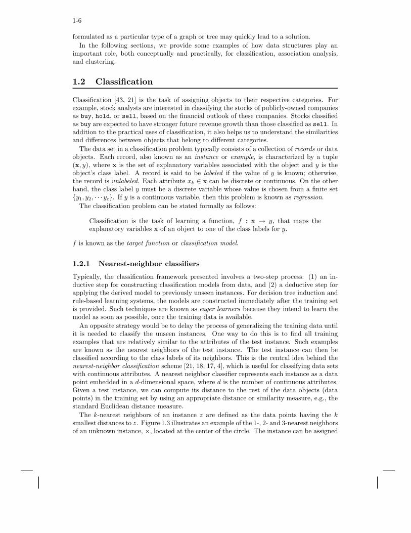
Research in data mining is motivated by a number of factors. In some cases, the goal is todevelop an approach with greater efficiency. For example, a current technique may workwell as long as all of the data can be held in main memory, but the size of data sets hasgrown to the point where this is no longer possible. In other cases, the goal may be todevelop an approach that is more flexible. For instance, the nature of the data may becontinually changing, and it may be necessary to develop a model of the data that can alsochange. As an example, network traffic varies in volume and kind, often over relativelyshort time periods. In yet other cases, the task is to obtain a more accurate model of thedata, i.e., one that takes into account additional factors that are common in many realworld situations.

The development and success of new data mining techniques is heavily dependent onthe creation of the proper algorithms and data structures to address the needs such asthose just described: efficiency, flexibility, and more accurate models. (This is not to saythat system or applications issues are unimportant.) Sometimes, currently existing datastructures and algorithms can be directly applied, e.g., data access methods can be used toefficiently organize and retrieve data. However, since currently existing data structures andalgorithms were typically not designed with data mining tasks in mind, it is frequently thecase that some modifications, enhancements, or completely new approaches are needed, i.e.,new work in data structures and algorithms is needed. We would emphasize, though, thatsometimes it is the concepts and viewpoints associated with currently existing algorithmsand data structures that are the most useful. Thus, the realization that a problem can be

1-6

formulated as a particular type of a graph or tree may quickly lead to a solution.

In the following sections, we provide some examples of how data structures play animportant role, both conceptually and practically, for classification, association analysis,and clustering.

1.2 Classification

Classification [43, 21] is the task of assigning objects to their respective categories. Forexample, stock analysts are interested in classifying the stocks of publicly-owned companiesas buy, hold, or sell, based on the financial outlook of these companies. Stocks classifiedas buy are expected to have stronger future revenue growth than those classified as sell. Inaddition to the practical uses of classification, it also helps us to understand the similaritiesand differences between objects that belong to different categories.

The data set in a classification problem typically consists of a collection of records or dataobjects. Each record, also known as an instance or example, is characterized by a tuple(x, y), where x is the set of explanatory variables associated with the object and y is theobject’s class label. A record is said to be labeled if the value of y is known; otherwise,the record is unlabeled. Each attribute xk ∈ x can be discrete or continuous. On the otherhand, the class label y must be a discrete variable whose value is chosen from a finite set{y1, y2, · · · yc}. If y is a continuous variable, then this problem is known as regression.

The classification problem can be stated formally as follows:

Classification is the task of learning a function, f : x → y, that maps theexplanatory variables x of an object to one of the class labels for y.

f is known as the target function or classification model.

1.2.1 Nearest-neighbor classifiers

Typically, the classification framework presented involves a two-step process: (1) an in-ductive step for constructing classification models from data, and (2) a deductive step forapplying the derived model to previously unseen instances. For decision tree induction andrule-based learning systems, the models are constructed immediately after the training setis provided. Such techniques are known as eager learners because they intend to learn themodel as soon as possible, once the training data is available.

An opposite strategy would be to delay the process of generalizing the training data untilit is needed to classify the unseen instances. One way to do this is to find all trainingexamples that are relatively similar to the attributes of the test instance. Such examplesare known as the nearest neighbors of the test instance. The test instance can then beclassified according to the class labels of its neighbors. This is the central idea behind thenearest-neighbor classification scheme [21, 18, 17, 4], which is useful for classifying data setswith continuous attributes. A nearest neighbor classifier represents each instance as a datapoint embedded in a d-dimensional space, where d is the number of continuous attributes.Given a test instance, we can compute its distance to the rest of the data objects (datapoints) in the training set by using an appropriate distance or similarity measure, e.g., thestandard Euclidean distance measure.

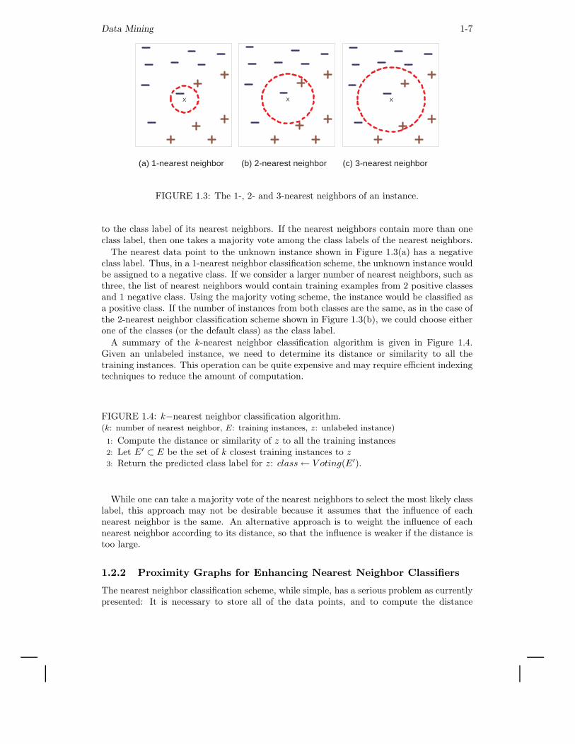
The k-nearest neighbors of an instance z are defined as the data points having the ksmallest distances to z. Figure 1.3 illustrates an example of the 1-, 2- and 3-nearest neighborsof an unknown instance, ×, located at the center of the circle. The instance can be assigned

Data Mining 1-7

X X X

(a) 1-nearest neighbor (b) 2-nearest neighbor (c) 3-nearest neighbor

FIGURE 1.3: The 1-, 2- and 3-nearest neighbors of an instance.

to the class label of its nearest neighbors. If the nearest neighbors contain more than oneclass label, then one takes a majority vote among the class labels of the nearest neighbors.

The nearest data point to the unknown instance shown in Figure 1.3(a) has a negativeclass label. Thus, in a 1-nearest neighbor classification scheme, the unknown instance wouldbe assigned to a negative class. If we consider a larger number of nearest neighbors, such asthree, the list of nearest neighbors would contain training examples from 2 positive classesand 1 negative class. Using the majority voting scheme, the instance would be classified asa positive class. If the number of instances from both classes are the same, as in the case ofthe 2-nearest neighbor classification scheme shown in Figure 1.3(b), we could choose eitherone of the classes (or the default class) as the class label.

A summary of the k-nearest neighbor classification algorithm is given in Figure 1.4.Given an unlabeled instance, we need to determine its distance or similarity to all thetraining instances. This operation can be quite expensive and may require efficient indexingtechniques to reduce the amount of computation.

FIGURE 1.4: k−nearest neighbor classification algorithm.(k: number of nearest neighbor, E: training instances, z: unlabeled instance)

1: Compute the distance or similarity of z to all the training instances2: Let E′ ⊂ E be the set of k closest training instances to z3: Return the predicted class label for z: class← V oting(E′).

While one can take a majority vote of the nearest neighbors to select the most likely classlabel, this approach may not be desirable because it assumes that the influence of eachnearest neighbor is the same. An alternative approach is to weight the influence of eachnearest neighbor according to its distance, so that the influence is weaker if the distance istoo large.

1.2.2 Proximity Graphs for Enhancing Nearest Neighbor Classifiers

The nearest neighbor classification scheme, while simple, has a serious problem as currentlypresented: It is necessary to store all of the data points, and to compute the distance

1-8

between an object to be classified and all of these stored objects. If the set of original datapoints is large, then this can be a significant computational burden. Hence, a considerableamount of research has been conducted into strategies to alleviate this problem.

There are two general strategies for addressing the problem just discussed:

Condensing The idea is that we can often eliminate many of the data points with-out affecting classification performance, or without affecting it very much. Forinstance, if a data object is in the ‘middle’ of a group of other objects with thesame class, then its elimination will likely have no effect on the nearest neighborclassifier.

Editing Often, the classification performance of a nearest neighbor classifier can beenhanced by deleting certain data points. More specifically, if a given object iscompared to its nearest neighbors and most of them are of another class (i.e., ifthe points that would be used to classify the given point are of another class),then deleting the given object will often improve classifier performance.

While various approaches to condensing and editing points to improve the performanceof nearest neighbor classifiers have been proposed, there has been a considerable amountof work that approaches this problem from the viewpoint of computational geometry, espe-cially proximity graphs [49]. Proximity graphs include nearest neighbor graphs, minimumspanning trees, relative neighborhood graphs, Gabriel graphs, and the Delaunay triangula-tion [35]. We can only indicate briefly the usefulness of this approach, and refer the readerto [49] for an in depth discussion.

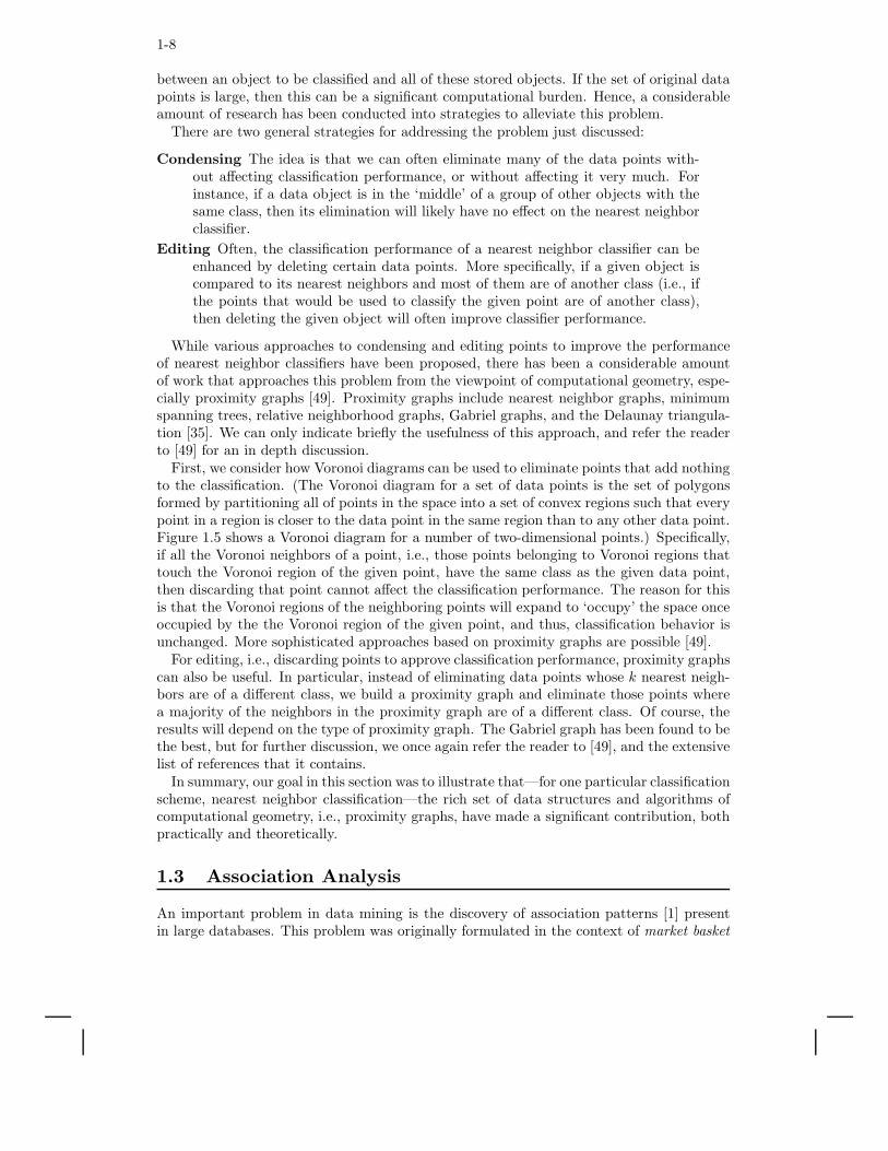
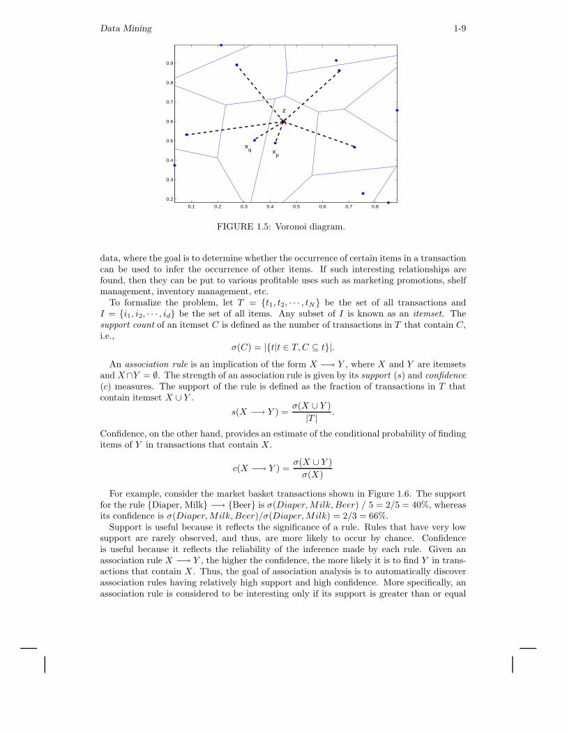
First, we consider how Voronoi diagrams can be used to eliminate points that add nothingto the classification. (The Voronoi diagram for a set of data points is the set of polygonsformed by partitioning all of points in the space into a set of convex regions such that everypoint in a region is closer to the data point in the same region than to any other data point.Figure 1.5 shows a Voronoi diagram for a number of two-dimensional points.) Specifically,if all the Voronoi neighbors of a point, i.e., those points belonging to Voronoi regions thattouch the Voronoi region of the given point, have the same class as the given data point,then discarding that point cannot affect the classification performance. The reason for thisis that the Voronoi regions of the neighboring points will expand to ‘occupy’ the space onceoccupied by the the Voronoi region of the given point, and thus, classification behavior isunchanged. More sophisticated approaches based on proximity graphs are possible [49].

For editing, i.e., discarding points to approve classification performance, proximity graphscan also be useful. In particular, instead of eliminating data points whose k nearest neigh-bors are of a different class, we build a proximity graph and eliminate those points wherea majority of the neighbors in the proximity graph are of a different class. Of course, theresults will depend on the type of proximity graph. The Gabriel graph has been found to bethe best, but for further discussion, we once again refer the reader to [49], and the extensivelist of references that it contains.

In summary, our goal in this section was to illustrate that—for one particular classificationscheme, nearest neighbor classification—the rich set of data structures and algorithms ofcomputational geometry, i.e., proximity graphs, have made a significant contribution, bothpractically and theoretically.

1.3 Association Analysis

An important problem in data mining is the discovery of association patterns [1] presentin large databases. This problem was originally formulated in the context of market basket

Data Mining 1-9

0.1 0.2 0.3 0.4 0.5 0.6 0.7 0.8

0.2

0.3

0.4

0.5

0.6

0.7

0.8

0.9

xp

xq

z

FIGURE 1.5: Voronoi diagram.

data, where the goal is to determine whether the occurrence of certain items in a transactioncan be used to infer the occurrence of other items. If such interesting relationships arefound, then they can be put to various profitable uses such as marketing promotions, shelfmanagement, inventory management, etc.

To formalize the problem, let T = {t1, t2, · · · , tN} be the set of all transactions andI = {i1, i2, · · · , id} be the set of all items. Any subset of I is known as an itemset. Thesupport count of an itemset C is defined as the number of transactions in T that contain C,i.e.,

σ(C) = |{t|t ∈ T, C ⊆ t}|.

An association rule is an implication of the form X −→ Y , where X and Y are itemsetsand X∩Y = ∅. The strength of an association rule is given by its support (s) and confidence(c) measures. The support of the rule is defined as the fraction of transactions in T thatcontain itemset X ∪ Y .

s(X −→ Y ) =σ(X ∪ Y )

|T |.

Confidence, on the other hand, provides an estimate of the conditional probability of findingitems of Y in transactions that contain X .

c(X −→ Y ) =σ(X ∪ Y )

σ(X)

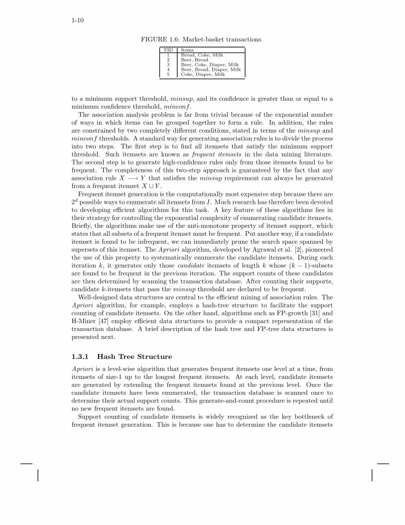
For example, consider the market basket transactions shown in Figure 1.6. The supportfor the rule {Diaper, Milk} −→ {Beer} is σ(Diaper, Milk, Beer) / 5 = 2/5 = 40%, whereasits confidence is σ(Diaper, Milk, Beer)/σ(Diaper, Milk) = 2/3 = 66%.

Support is useful because it reflects the significance of a rule. Rules that have very lowsupport are rarely observed, and thus, are more likely to occur by chance. Confidenceis useful because it reflects the reliability of the inference made by each rule. Given anassociation rule X −→ Y , the higher the confidence, the more likely it is to find Y in trans-actions that contain X . Thus, the goal of association analysis is to automatically discoverassociation rules having relatively high support and high confidence. More specifically, anassociation rule is considered to be interesting only if its support is greater than or equal

1-10

FIGURE 1.6: Market-basket transactions

TID Items1 Bread, Coke, Milk2 Beer, Bread3 Beer, Coke, Diaper, Milk4 Beer, Bread, Diaper, Milk5 Coke, Diaper, Milk

to a minimum support threshold, minsup, and its confidence is greater than or equal to aminimum confidence threshold, minconf .

The association analysis problem is far from trivial because of the exponential numberof ways in which items can be grouped together to form a rule. In addition, the rulesare constrained by two completely different conditions, stated in terms of the minsup andminconf thresholds. A standard way for generating association rules is to divide the processinto two steps. The first step is to find all itemsets that satisfy the minimum supportthreshold. Such itemsets are known as frequent itemsets in the data mining literature.The second step is to generate high-confidence rules only from those itemsets found to befrequent. The completeness of this two-step approach is guaranteed by the fact that anyassociation rule X −→ Y that satisfies the minsup requirement can always be generatedfrom a frequent itemset X ∪ Y .

Frequent itemset generation is the computationally most expensive step because there are2d possible ways to enumerate all itemsets from I. Much research has therefore been devotedto developing efficient algorithms for this task. A key feature of these algorithms lies intheir strategy for controlling the exponential complexity of enumerating candidate itemsets.Briefly, the algorithms make use of the anti-monotone property of itemset support, whichstates that all subsets of a frequent itemset must be frequent. Put another way, if a candidateitemset is found to be infrequent, we can immediately prune the search space spanned bysupersets of this itemset. The Apriori algorithm, developed by Agrawal et al. [2], pioneeredthe use of this property to systematically enumerate the candidate itemsets. During eachiteration k, it generates only those candidate itemsets of length k whose (k − 1)-subsetsare found to be frequent in the previous iteration. The support counts of these candidatesare then determined by scanning the transaction database. After counting their supports,candidate k-itemsets that pass the minsup threshold are declared to be frequent.

Well-designed data structures are central to the efficient mining of association rules. TheApriori algorithm, for example, employs a hash-tree structure to facilitate the supportcounting of candidate itemsets. On the other hand, algorithms such as FP-growth [31] andH-Miner [47] employ efficient data structures to provide a compact representation of thetransaction database. A brief description of the hash tree and FP-tree data structures ispresented next.

1.3.1 Hash Tree Structure

Apriori is a level-wise algorithm that generates frequent itemsets one level at a time, fromitemsets of size-1 up to the longest frequent itemsets. At each level, candidate itemsetsare generated by extending the frequent itemsets found at the previous level. Once thecandidate itemsets have been enumerated, the transaction database is scanned once todetermine their actual support counts. This generate-and-count procedure is repeated untilno new frequent itemsets are found.

Support counting of candidate itemsets is widely recognized as the key bottleneck offrequent itemset generation. This is because one has to determine the candidate itemsets

Data Mining 1-11

2,5,8

1,4,7 3,6,9

Hash Function

1 2 3 5 6

3 4 5 3 5 6

2 3 5 6

3 5 6

5 6

1 +

2 +

3 +

2 3 4

Transaction

Candidate Hash Tree

3 6 71 3 61 4 5

1 2 4 1 2 5 1 5 9

6 8 9

3 5 7

4 5 7 4 5 8

3 6 8

5 6 7

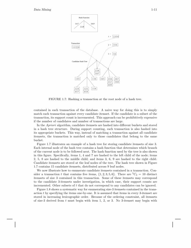
FIGURE 1.7: Hashing a transaction at the root node of a hash tree.

contained in each transaction of the database. A naive way for doing this is to simplymatch each transaction against every candidate itemset. If the candidate is a subset of thetransaction, its support count is incremented. This approach can be prohibitively expensiveif the number of candidates and number of transactions are large.

In the Apriori algorithm, candidate itemsets are hashed into different buckets and storedin a hash tree structure. During support counting, each transaction is also hashed intoits appropriate buckets. This way, instead of matching a transaction against all candidateitemsets, the transaction is matched only to those candidates that belong to the samebucket.

Figure 1.7 illustrates an example of a hash tree for storing candidate itemsets of size 3.Each internal node of the hash tree contains a hash function that determines which branchof the current node is to be followed next. The hash function used by the tree is also shownin this figure. Specifically, items 1, 4 and 7 are hashed to the left child of the node; items2, 5, 8 are hashed to the middle child; and items 3, 6, 9 are hashed to the right child.Candidate itemsets are stored at the leaf nodes of the tree. The hash tree shown in Figure1.7 contains 15 candidate itemsets, distributed across 9 leaf nodes.

We now illustrate how to enumerate candidate itemsets contained in a transaction. Con-sider a transaction t that contains five items, {1, 2, 3, 5, 6}. There are 5C3 = 10 distinctitemsets of size 3 contained in this transaction. Some of these itemsets may correspondto the candidate 3-itemsets under investigation, in which case, their support counts areincremented. Other subsets of t that do not correspond to any candidates can be ignored.

Figure 1.8 shows a systematic way for enumerating size-3 itemsets contained in the trans-action t by specifying the items one-by-one. It is assumed that items in every 3-itemset arestored in increasing lexicographic order. Because of the ordering constraint, all itemsetsof size-3 derived from t must begin with item 1, 2, or 3. No 3-itemset may begin with

1-12

1 2 3 5 6

Transaction, t

2 3 5 6 1 3 5 6 2

5 6 1 3 3 5 6 1 2 6 1 5 5 6 2 3 6 2 5

5 6 3

1 2 3 1 2 5 1 2 6

1 3 5 1 3 6

1 5 6 2 3 5 2 3 6

2 5 6 3 5 6

Subsets of 3 items

Level 1

Level 2

Level 3

6 3 5

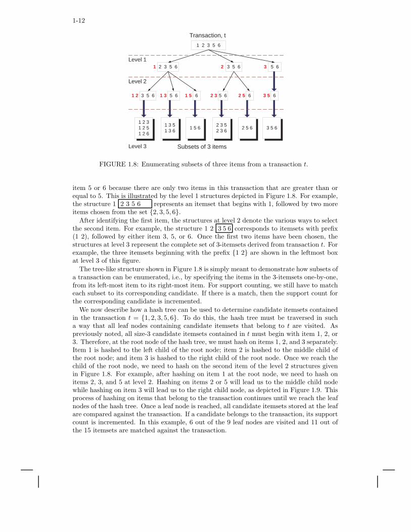
FIGURE 1.8: Enumerating subsets of three items from a transaction t.

item 5 or 6 because there are only two items in this transaction that are greater than orequal to 5. This is illustrated by the level 1 structures depicted in Figure 1.8. For example,the structure 1 2 3 5 6 represents an itemset that begins with 1, followed by two moreitems chosen from the set {2, 3, 5, 6}.

After identifying the first item, the structures at level 2 denote the various ways to selectthe second item. For example, the structure 1 2 3 5 6 corresponds to itemsets with prefix(1 2), followed by either item 3, 5, or 6. Once the first two items have been chosen, thestructures at level 3 represent the complete set of 3-itemsets derived from transaction t. Forexample, the three itemsets beginning with the prefix {1 2} are shown in the leftmost boxat level 3 of this figure.

The tree-like structure shown in Figure 1.8 is simply meant to demonstrate how subsets ofa transaction can be enumerated, i.e., by specifying the items in the 3-itemsets one-by-one,from its left-most item to its right-most item. For support counting, we still have to matcheach subset to its corresponding candidate. If there is a match, then the support count forthe corresponding candidate is incremented.

We now describe how a hash tree can be used to determine candidate itemsets containedin the transaction t = {1, 2, 3, 5, 6}. To do this, the hash tree must be traversed in sucha way that all leaf nodes containing candidate itemsets that belong to t are visited. Aspreviously noted, all size-3 candidate itemsets contained in t must begin with item 1, 2, or3. Therefore, at the root node of the hash tree, we must hash on items 1, 2, and 3 separately.Item 1 is hashed to the left child of the root node; item 2 is hashed to the middle child ofthe root node; and item 3 is hashed to the right child of the root node. Once we reach thechild of the root node, we need to hash on the second item of the level 2 structures givenin Figure 1.8. For example, after hashing on item 1 at the root node, we need to hash onitems 2, 3, and 5 at level 2. Hashing on items 2 or 5 will lead us to the middle child nodewhile hashing on item 3 will lead us to the right child node, as depicted in Figure 1.9. Thisprocess of hashing on items that belong to the transaction continues until we reach the leafnodes of the hash tree. Once a leaf node is reached, all candidate itemsets stored at the leafare compared against the transaction. If a candidate belongs to the transaction, its supportcount is incremented. In this example, 6 out of the 9 leaf nodes are visited and 11 out ofthe 15 itemsets are matched against the transaction.

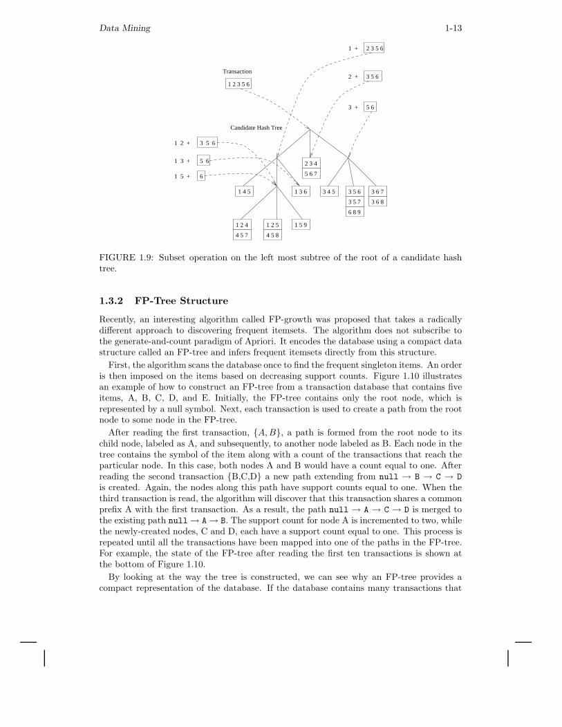
Data Mining 1-13

1 2 3 5 6

3 4 5 3 5 6

3 5 61 2 +

1 3 + 5 6

1 5 + 6

2 3 5 6

3 5 6

5 6

1 +

2 +

3 +

2 3 4

Transaction

3 6 71 3 61 4 5

1 2 4 1 2 5 1 5 9

6 8 9

3 5 7

4 5 7 4 5 8

3 6 8

5 6 7

Candidate Hash Tree

FIGURE 1.9: Subset operation on the left most subtree of the root of a candidate hashtree.

1.3.2 FP-Tree Structure

Recently, an interesting algorithm called FP-growth was proposed that takes a radicallydifferent approach to discovering frequent itemsets. The algorithm does not subscribe tothe generate-and-count paradigm of Apriori. It encodes the database using a compact datastructure called an FP-tree and infers frequent itemsets directly from this structure.

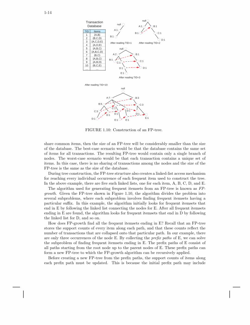
First, the algorithm scans the database once to find the frequent singleton items. An orderis then imposed on the items based on decreasing support counts. Figure 1.10 illustratesan example of how to construct an FP-tree from a transaction database that contains fiveitems, A, B, C, D, and E. Initially, the FP-tree contains only the root node, which isrepresented by a null symbol. Next, each transaction is used to create a path from the rootnode to some node in the FP-tree.

After reading the first transaction, {A, B}, a path is formed from the root node to itschild node, labeled as A, and subsequently, to another node labeled as B. Each node in thetree contains the symbol of the item along with a count of the transactions that reach theparticular node. In this case, both nodes A and B would have a count equal to one. Afterreading the second transaction {B,C,D} a new path extending from null → B → C → D

is created. Again, the nodes along this path have support counts equal to one. When thethird transaction is read, the algorithm will discover that this transaction shares a commonprefix A with the first transaction. As a result, the path null → A → C → D is merged tothe existing path null→ A→ B. The support count for node A is incremented to two, whilethe newly-created nodes, C and D, each have a support count equal to one. This process isrepeated until all the transactions have been mapped into one of the paths in the FP-tree.For example, the state of the FP-tree after reading the first ten transactions is shown atthe bottom of Figure 1.10.

By looking at the way the tree is constructed, we can see why an FP-tree provides acompact representation of the database. If the database contains many transactions that

1-14

TID Items 1 {A,B} 2 {B,C,D} 3 {A,C,D,E} 4 {A,D,E} 5 {A,B,C} 6 {A,B,C,D} 7 {B,C} 8 {A,B,C} 9 {A,B,D} 10 {B,C,E} … …

Transaction Database

After reading TID=1

null

A:1

B:1

After reading TID=2

null

A:1

B:1

B:1

C:1

D:1

After reading TID=3

null

A:2

B:1

B:1

C:1

D:1

C:1

D:1

After reading TID=10:

E:1

null

A:7 B:3

C:3

D:1

C:1

D:1

E:1

B:5

C:3

D:1

D:1

D:1

E:1 E:1

FIGURE 1.10: Construction of an FP-tree.

share common items, then the size of an FP-tree will be considerably smaller than the sizeof the database. The best-case scenario would be that the database contains the same setof items for all transactions. The resulting FP-tree would contain only a single branch ofnodes. The worst-case scenario would be that each transaction contains a unique set ofitems. In this case, there is no sharing of transactions among the nodes and the size of theFP-tree is the same as the size of the database.

During tree construction, the FP-tree structure also creates a linked-list access mechanismfor reaching every individual occurrence of each frequent item used to construct the tree.In the above example, there are five such linked lists, one for each item, A, B, C, D, and E.

The algorithm used for generating frequent itemsets from an FP-tree is known as FP-growth. Given the FP-tree shown in Figure 1.10, the algorithm divides the problem intoseveral subproblems, where each subproblem involves finding frequent itemsets having aparticular suffix. In this example, the algorithm initially looks for frequent itemsets thatend in E by following the linked list connecting the nodes for E. After all frequent itemsetsending in E are found, the algorithm looks for frequent itemsets that end in D by followingthe linked list for D, and so on.

How does FP-growth find all the frequent itemsets ending in E? Recall that an FP-treestores the support counts of every item along each path, and that these counts reflect thenumber of transactions that are collapsed onto that particular path. In our example, thereare only three occurrences of the node E. By collecting the prefix paths of E, we can solvethe subproblem of finding frequent itemsets ending in E. The prefix paths of E consist ofall paths starting from the root node up to the parent nodes of E. These prefix paths canform a new FP-tree to which the FP-growth algorithm can be recursively applied.

Before creating a new FP-tree from the prefix paths, the support counts of items alongeach prefix path must be updated. This is because the initial prefix path may include

Data Mining 1-15

several transactions that do not contain the item E. For this reason, the support count ofeach item along the prefix path must be adjusted to have the same count as node E forthat particular path. After updating the counts along the prefix paths of E, some itemsmay no longer be frequent, and thus, must be removed from further consideration (as far asour new subproblem is concerned). An FP-tree of the prefix paths is then constructed byremoving the infrequent items. This recursive process of breaking the problem into smallersubproblems will continue until the subproblem involves only a single item. If the supportcount of this item is greater than the minimum support threshold, then the label of thisitem will be returned by the FP-growth algorithm. The returned label is appended as aprefix to the frequent itemset ending in E.

1.4 Clustering

Cluster analysis [33, 39, 6, 7] groups data objects based on information found in the datathat describes the objects and their relationships. The goal is that the objects in a groupbe similar (or related) to one another and different from (or unrelated to) the objects inother groups. The greater the similarity (or homogeneity) within a group, and the greaterthe difference between groups, the ‘better’ or more distinct the clustering.

1.4.1 Hierarchical and Partitional Clustering

The most commonly made distinction between clustering techniques is whether the resultingclusters are nested or unnested or, in more traditional terminology, whether a set of clustersis hierarchical or partitional. A partitional or unnested set of clusters is simply a divisionof the set of data objects into non-overlapping subsets (clusters) such that each data objectis in exactly one subset, i.e., a partition of the data objects. The most common partitionalclustering algorithm is K-means, whose operation is described by the psuedo-code in Figure1.11. (K is a user specified parameter, i.e., the number of clusters desired, and a centroidis typically the mean or median of the points in a cluster.)

FIGURE 1.11: Basic K-means Algorithm.

1: Initialization: Select K points as the initial centroids.2: repeat

3: Form K clusters by assigning all points to the closest centroid.4: Recompute the centroid of each cluster.5: until The centroids do not change

A hierarchical or nested clustering is a set of nested clusters organized as a hierarchicaltree, where the leaves of the tree are singleton clusters of individual data objects, and wherethe cluster associated with each interior node of the tree is the union of the clusters asso-ciated with its child nodes. Typically, hierarchical clustering proceeds in an agglomerativemanner, i.e., starting with each point as a cluster, we repeatedly merge the closest clusters,until only one cluster remains. A wide variety of methods can be used to define the distancebetween two clusters, but this distance is typically defined in terms of the distances betweenpairs of points in different clusters. For instance, the distance between clusters may be theminimum distance between any pair of points, the maximum distance, or the average dis-

1-16

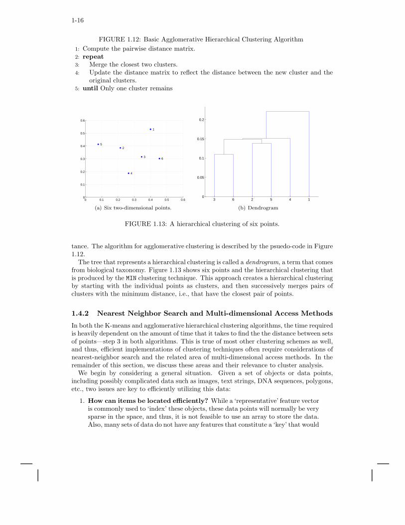
FIGURE 1.12: Basic Agglomerative Hierarchical Clustering Algorithm

1: Compute the pairwise distance matrix.2: repeat

3: Merge the closest two clusters.4: Update the distance matrix to reflect the distance between the new cluster and the

original clusters.5: until Only one cluster remains

0 0.1 0.2 0.3 0.4 0.5 0.60

0.1

0.2

0.3

0.4

0.5

0.6

1

2

3

4

5

6

(a) Six two-dimensional points.

3 6 2 5 4 10

0.05

0.1

0.15

0.2

(b) Dendrogram

FIGURE 1.13: A hierarchical clustering of six points.

tance. The algorithm for agglomerative clustering is described by the psuedo-code in Figure1.12.

The tree that represents a hierarchical clustering is called a dendrogram, a term that comesfrom biological taxonomy. Figure 1.13 shows six points and the hierarchical clustering thatis produced by the MIN clustering technique. This approach creates a hierarchical clusteringby starting with the individual points as clusters, and then successively merges pairs ofclusters with the minimum distance, i.e., that have the closest pair of points.

1.4.2 Nearest Neighbor Search and Multi-dimensional Access Methods

In both the K-means and agglomerative hierarchical clustering algorithms, the time requiredis heavily dependent on the amount of time that it takes to find the the distance between setsof points—step 3 in both algorithms. This is true of most other clustering schemes as well,and thus, efficient implementations of clustering techniques often require considerations ofnearest-neighbor search and the related area of multi-dimensional access methods. In theremainder of this section, we discuss these areas and their relevance to cluster analysis.

We begin by considering a general situation. Given a set of objects or data points,including possibly complicated data such as images, text strings, DNA sequences, polygons,etc., two issues are key to efficiently utilizing this data:

1. How can items be located efficiently? While a ‘representative’ feature vectoris commonly used to ‘index’ these objects, these data points will normally be verysparse in the space, and thus, it is not feasible to use an array to store the data.Also, many sets of data do not have any features that constitute a ‘key’ that would

Data Mining 1-17

allow the data to be accessed using standard and efficient database techniques.

2. How can similarity queries be efficiently conducted? Many applications,including clustering, require the nearest neighbor (or the k nearest neighbors) of apoint. For instance, the clustering techniques DBSCAN [24] and Chameleon [37]will have a time complexity of O(n2) unless they can utilize data structures andalgorithms that allow the nearest neighbors of a point to be located efficiently.As a non-clustering example of an application of similarity queries, a user maywant to find all the pictures similar to a particular photograph in a database ofphotographs.

Techniques for nearest-neighbor search are often discussed in papers describing multi-dimensional access methods or spatial access methods, although strictly speaking the topicof multi-dimensional access methods is broader than nearest-neighbor search since it ad-dresses all of the many different types of queries and operations that a user might wantto perform on multi-dimensional data. A large amount of work has been done in the areaof nearest neighbor search and multi-dimensional access methods. Examples of such workinclude the kdb tree [48, 14], the R [28] tree, the R* tree [8], the SS-tree [34], the SR-tree[38], the X-tree [11], the GNAT tree [13], the M-tree [16], the TV tree [41], the hB tree [42],the “pyramid technique” [10], and the ‘hybrid’ tree [15]. A good survey of nearest-neighborsearch, albeit from the slightly more general perspective of multi-dimensional access meth-ods is given by [26].

As indicated by the prevalence of the word ‘tree’ in the preceding references, a commonapproach for nearest neighbor search is to create tree-based structures, such that the ‘close-ness’ of the data increases as the tree is traversed from top to bottom. Thus, the nodestowards the bottom of the tree and their children can often be regarded as representing‘clusters’ of data that are relatively cohesive. In the reverse directions, we also view clus-tering as being potentially useful for finding nearest neighbors. Indeed, one of the simplesttechniques for generating a nearest neighbor tree is to cluster the data into a set of clustersand then, recursively break each cluster into subclusters until the subclusters consist ofindividual points. The resulting cluster tree tree consists of the clusters generated along theway. Regardless of how a nearest neighbor search tree is obtained, the general approach forperforming a k-nearest-neighbor query is given by the algorithm in Figure 1.14.

This seems fairly straightforward and, thus it seems as though nearest neighbor treesshould useful for clustering data, or conversely, that clustering would be a practical way tofind nearest neighbors based on the results of clustering. However, there are some problems.

Goal Mismatch One of the goals of many nearest-neighbor tree techniques is to serveas efficient secondary storage based access methods for non-traditional databases,e.g., spatial databases, multimedia databases, document databases, etc. Becauseof requirements related to page size and efficient page utilization, ‘natural’ clus-ters may be split across pages or nodes. Nonetheless, data is normally highly‘clustered’ and this can be used for actual clustering as shown in [25], which usesan R* tree to improve the efficiency of a clustering algorithm introduced in [46].

Problems with High-dimensional Data Because of the nature of nearest-neighbortrees, the tree search involved is a branch-and-bound technique and needs tosearch large parts of the tree, i.e., at any particular level, many children andtheir descendants may need to be examined. To see this, consider a point andall points that are within a given distance of it. This hyper-sphere (or hyper-rectangle in the case of multi-dimensional range queries) may very well cut acrossa number of nodes (clusters)—particularly if the point is on the edge of a cluster

1-18

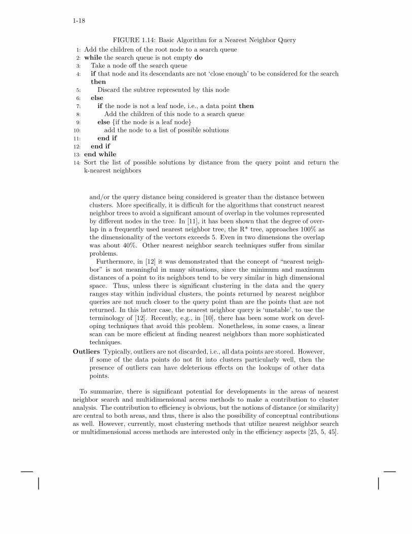
FIGURE 1.14: Basic Algorithm for a Nearest Neighbor Query

1: Add the children of the root node to a search queue2: while the search queue is not empty do

3: Take a node off the search queue4: if that node and its descendants are not ‘close enough’ to be considered for the search

then

5: Discard the subtree represented by this node6: else

7: if the node is not a leaf node, i.e., a data point then

8: Add the children of this node to a search queue9: else {if the node is a leaf node}

10: add the node to a list of possible solutions11: end if

12: end if

13: end while

14: Sort the list of possible solutions by distance from the query point and return thek-nearest neighbors

and/or the query distance being considered is greater than the distance betweenclusters. More specifically, it is difficult for the algorithms that construct nearestneighbor trees to avoid a significant amount of overlap in the volumes representedby different nodes in the tree. In [11], it has been shown that the degree of over-lap in a frequently used nearest neighbor tree, the R* tree, approaches 100% asthe dimensionality of the vectors exceeds 5. Even in two dimensions the overlapwas about 40%. Other nearest neighbor search techniques suffer from similarproblems.

Furthermore, in [12] it was demonstrated that the concept of “nearest neigh-bor” is not meaningful in many situations, since the minimum and maximumdistances of a point to its neighbors tend to be very similar in high dimensionalspace. Thus, unless there is significant clustering in the data and the queryranges stay within individual clusters, the points returned by nearest neighborqueries are not much closer to the query point than are the points that are notreturned. In this latter case, the nearest neighbor query is ‘unstable’, to use theterminology of [12]. Recently, e.g., in [10], there has been some work on devel-oping techniques that avoid this problem. Nonetheless, in some cases, a linearscan can be more efficient at finding nearest neighbors than more sophisticatedtechniques.

Outliers Typically, outliers are not discarded, i.e., all data points are stored. However,if some of the data points do not fit into clusters particularly well, then thepresence of outliers can have deleterious effects on the lookups of other datapoints.

To summarize, there is significant potential for developments in the areas of nearestneighbor search and multidimensional access methods to make a contribution to clusteranalysis. The contribution to efficiency is obvious, but the notions of distance (or similarity)are central to both areas, and thus, there is also the possibility of conceptual contributionsas well. However, currently, most clustering methods that utilize nearest neighbor searchor multidimensional access methods are interested only in the efficiency aspects [25, 5, 45].

Data Mining 1-19

1.5 Conclusion

In this chapter we have provided some examples to indicate the role that data structuresplay in data mining. For classification, we indicated how proximity graphs can play animportant role in understanding and improving the performance of nearest neighbor classi-fiers. For association analysis, we showed how data structures are currently used to addressthe exponential complexity of the problem. For clustering, we explored its connection tonearest neighbor search and multi-dimensional access methods—a connection that has onlybeen modestly exploited.

Data mining is a rapidly evolving field, with new problems continually arising, and oldproblems being looked at in the light of new developments. These developments pose newchallenges in the areas of data structures and algorithms. Some of the most promising areasin current data mining research include multi-relational data mining [23, 20, 32], miningstreams of data [19], privacy preserving data mining [3], and mining data with complicatedstructures or behaviors, e.g., graphs [32, 40] and link analysis [36, 44].

Acknowledgement

This work was partially supported by NASA grant # NCC 2 1231 and by the Army HighPerformance Computing Research Center under the auspices of the Department of theArmy, Army Research Laboratory cooperative agreement number DAAD19-01-2-0014. Thecontent of this work does not necessarily reflect the position or policy of the governmentand no official endorsement should be inferred. Access to computing facilities was providedby the AHPCRC and the Minnesota Supercomputing Institute.

References

[1] R. Agrawal, T. Imielinski, and A. Swami. Mining association rules between sets of

items in large databases. In Proc. ACM SIGMOD Intl. Conf. Management of Data,

pages 207–216, Washington D.C., USA, 1993.

[2] R. Agrawal and R. Srikant. Fast algorithms for mining association rules. In Proc. ofthe 20th VLDB Conference, pages 487–499, Santiago, Chile, 1994.

[3] R. Agrawal and R. Srikant. Privacy-preserving data mining. In Proc. of the ACMSIGMOD Conference on Management of Data, pages 439–450. ACM Press, May

2000.

[4] D. Aha. A study of instance-based algorithms for supervised learning tasks: math-ematical, empirical, and psychological evaluations. PhD thesis, University of Cali-

fornia, Irvine, 1990.

[5] Alsabti, Ranka, and Singh. An efficient parallel algorithm for high dimensional sim-

ilarity join. In IPPS: 11th International Parallel Processing Symposium. IEEE

Computer Society Press, 1998.

[6] M. R. Anderberg. Cluster Analysis for Applications. Academic Press, New York,

December 1973.

[7] P. Arabie, L. Hubert, and G. De Soete. An overview of combinatorial data analysis. In

P. Arabie, L. Hubert, and G. De Soete, editors, Clustering and Classification, pages

188–217. World Scientific, Singapore, January 1996.

[8] N. Beckmann, H.-P. Kriegel, R. Schneider, and B. Seeger. The r*-tree: an efficient

1-20

and robust access method for points and rectangles. In Proceedings of the 1990 ACMSIGMOD international conference on Management of data, pages 322–331. ACM

Press, 1990.

[9] R. Bellman. Adaptive Control Processes: A Guided Tour. Princeton University

Press, 1961.

[10] S. Berchtold, C. Bhm, and H.-P. Kriegal. The pyramid-technique: towards breaking

the curse of dimensionality. In Proceedings of the 1998 ACM SIGMOD internationalconference on Management of data, pages 142–153. ACM Press, 1998.

[11] S. Berchtold, D. A. Keim, and H.-P. Kriegel. The X-tree: An index structure for

high-dimensional data. In T. M. Vijayaraman, A. P. Buchmann, C. Mohan, and N. L.

Sarda, editors, Proceedings of the 22nd International Conference on Very LargeDatabases, pages 28–39, San Francisco, U.S.A., 1996. Morgan Kaufmann Publishers.

[12] K. Beyer, J. Goldstein, R. Ramakrishnan, and U. Shaft. When is “nearest neighbor”

meaningful? In Proceedings 7th International Conference on Database Theory(ICDT’99), pages 217–235, 1999.

[13] S. Brin. Near neighbor search in large metric spaces. In The VLDB Journal, pages

574–584, 1995.

[14] T. B. B. Yu, R. Orlandic, and J. Somavaram. KdbKD-tree: A compact kdb-tree struc-

ture for indexing multidimensional data. In Proceedings of the 2003 IEEE Inter-national Symposium on Information Technology (ITCC 2003). IEEE, April, 28-30,

2003.

[15] K. Chakrabarti and S. Mehrotra. The hybrid tree: An index structure for high di-

mensional feature spaces. In Proceedings of the 15th International Conference onData Engineering, 23-26 March 1999, Sydney, Austrialia, pages 440–447. IEEE

Computer Society, 1999.

[16] P. Ciaccia, M. Patella, and P. Zezula. M-tree: An efficient access method for similarity

search in metric spaces. In The VLDB Journal, pages 426–435, 1997.

[17] S. Cost and S. Salzberg. A weighted nearest neighbor algorithm for learning with

symbolic features. Machine Learning, 10:57–78, 1993.

[18] T. M. Cover and P. E. Hart. Nearest neighbor pattern classification. Knowledge BasedSystems, 8(6):373–389, 1995.

[19] P. Domingos and G. Hulten. A general framework for mining massive data streams.

Journal of Computational and Graphical Statistics, 12, 2003.

[20] P. Domingos. Prospects and challenges for multirelational data mining. SIGKDDExplorations, 5(1), July 2003.

[21] R. O. Duda, P. E. Hart, and D. G. Stork. Pattern Classification. John Wiley & Sons,

Inc., New York, second edition, 2001.

[22] M. H. Dunham. Data Mining: Introductory and Advanced Topics. Prentice Hall,

2002.

[23] S. Dzeroski and L. D. Raedt. Multi-relational data mining: The current frontiers.

SIGKDD Explorations, 5(1), July 2003.

[24] M. Ester, H.-P. Kriegel, J. Sander, and X. Xu. A density-based algorithm for dis-

covering clusters in large spatial databases with noise. In KDD96, pages 226–231,

1996.

[25] M. Ester, H.-P. Kriegel, and X. Xu. Knowledge discovery in large spatial databases:

focusing techniques for efficient class identification. In M. Egenhofer and J. Herring,

editors, Advances in Spatial Databases, 4th International Symposium, SSD’95, vol-

ume 951, pages 67–82, Portland, ME, 1995. Springer.

[26] V. Gaede and O. Gnther. Multidimensional access methods. ACM Computing Surveys(CSUR), 30(2):170–231, 1998.

Data Mining 1-21

[27] R. L. Grossman, C. Kamath, V. K. Philip Kegelmeyer, and R. R. Namburu, editors.

Data Mining for Scientific and Engineering Applications. Kluwer Academic Pub-

lishers, October 2001.

[28] A. Guttman. R-trees: a dynamic index structure for spatial searching. In Proceedingsof the 1984 ACM SIGMOD international conference on Management of data, pages

47–57. ACM Press, 1984.

[29] D. Hand, H. Mannila, and P. Smyth. Principles of Data Mining. MIT Press, 2001.

[30] J. Han and M. Kamber. Data Mining: Concepts and Techniques. Morgan Kaufmann

Publishers, San Francisco, 2001.

[31] J. Han, J. Pei, and Y. Yin. Mining frequent patterns without candidate generation.

In Proc. 2000 ACM-SIGMOD Int’l Conf on Management of Data (SIGMOD’00),Dallas, TX, May 2000.

[32] L. B. Holder and D. J. Cook. Graph-based relational learning: Current and future

directions. SIGKDD Explorations, 5(1), July 2003.

[33] A. K. Jain and R. C. Dubes. Algorithms for Clustering Data. Prentice Hall Advanced

Reference Series. Prentice Hall, Englewood Cliffs, New Jersey, March 1988.

[34] R. Jain and D. A. White. Similarity indexing with the ss-tree. In Proceedings of the12th International Conference on Data Engineering, pages 516–523, 1996.

[35] J. W. Jaromczyk and G. T. Toussaint. Relative neighborhood graphs and their rela-

tives. Proceedings of the IEEE, 80(9):1502–1517, September 1992.

[36] D. Jensen and J. Neville. Data mining in social networks. In National Academy ofSciences Symposium on Dynamic Social Network Analysis, 2002.

[37] G. Karypis, E.-H. Han, , and V. Kumar. Chameleon: Hierarchical clustering using

dynamic modeling. Computer, 32(8):68–75, 1999.

[38] N. Katayama and S. Satoh. The sr-tree: an index structure for high-dimensional

nearest neighbor queries. In Proceedings of the 1997 ACM SIGMOD internationalconference on Management of data, pages 369–380. ACM Press, 1997.

[39] L. Kaufman and P. J. Rousseeuw. Finding Groups in Data: An Introduction toCluster Analysis. Wiley Series in Probability and Statistics. John Wiley and Sons,

New York, Novemeber 1990.

[40] M. Kuramochi and G. Karypis. Frequent subgraph discovery. In The 2001 IEEEInternational Conference on Data Mining, pages 313–320, 2001.

[41] K.-I. Lin, H. V. Jagadish, and C. Faloutsos. The tv-tree: An index structure for

high-dimensional data. VLDB Journal, 3(4):517–542, 1994.

[42] D. B. Lomet and B. Salzberg. The hb-tree: a multiattribute indexing method with

good guaranteed performance. ACM Transactions on Database Systems (TODS),15(4):625–658, 1990.

[43] T. M. Mitchell. Machine Learning. McGraw-Hill, March 1997.

[44] D. Mladenic, M. Grobelnik, N. Milic-Frayling, S. Donoho, and T. D. (editors). Kdd

2003: Workshop on link analysis for detecting complex behavior, August 2003.

[45] F. Murtagh. Clustering in massive data sets. In J. Abello, P. M. Pardalos, and M. G. C.

Resende, editors, Handbook of Massive Data Sets, pages 501–543. Kluwer Academic

Publishers, Dordrecht, Netherlands, May 2002.

[46] R. T. Ng and J. Han. Efficient and effective clustering methods for spatial data mining.

In J. Bocca, M. Jarke, and C. Zaniolo, editors, 20th International Conference on VeryLarge Data Bases, September 12–15, 1994, Santiago, Chile proceedings, pages 144–

155, Los Altos, CA 94022, USA, 1994. Morgan Kaufmann Publishers.

[47] J. Pei, J. Han, H. Lu, S. Nishio, S. Tang, and D. Yang. H-mine: Hyperstructure mining

of frequent patterns in large databases. In Proc. 2001 Int’l Conf on Data Mining(ICDM’01), San Jose, CA, Nov 2001.

1-22

[48] J. T. Robinson. The k-d-b-tree: a search structure for large multidimensional dynamic

indexes. In Proceedings of the 1981 ACM SIGMOD international conference onManagement of data, pages 10–18. ACM Press, 1981.

[49] G. T. Toussaint. Proximity graphs for nearest neighbor decision rules: recent

progress. In Interface-2002, 34th Symposium on Computing and Statistics, Mon-treal, Canada, April 17-20 2002.

[50] I. H. Witten and E. Frank. Data Mining: Practical Machine Learning Tools andTechniques with Java Implementations. Morgan Kaufmann, 1999.