DATA-DRIVEN VERIFICATION A DISSERTATION SUBMITTED TO THE DEPARTMENT OF COMPUTER SCIENCE AND THE COMMITTEE ON GRADUATE STUDIES OF STANFORD UNIVERSITY IN PARTIAL FULFILLMENT OF THE REQUIREMENTS FOR THE DEGREE OF DOCTOR OF PHILOSOPHY Rahul Sharma January 2016

Welcome message from author
This document is posted to help you gain knowledge. Please leave a comment to let me know what you think about it! Share it to your friends and learn new things together.
Transcript
DATA-DRIVEN VERIFICATION
A DISSERTATION
SUBMITTED TO THE DEPARTMENT OF COMPUTER SCIENCE
AND THE COMMITTEE ON GRADUATE STUDIES
OF STANFORD UNIVERSITY
IN PARTIAL FULFILLMENT OF THE REQUIREMENTS
FOR THE DEGREE OF
DOCTOR OF PHILOSOPHY
Rahul Sharma
January 2016

c© Copyright by Rahul Sharma 2016
All Rights Reserved
ii

I certify that I have read this dissertation and that, in my opinion, it is fully adequate
in scope and quality as a dissertation for the degree of Doctor of Philosophy.
(Alex Aiken) Principal Adviser
I certify that I have read this dissertation and that, in my opinion, it is fully adequate
in scope and quality as a dissertation for the degree of Doctor of Philosophy.
(David L. Dill)
I certify that I have read this dissertation and that, in my opinion, it is fully adequate
in scope and quality as a dissertation for the degree of Doctor of Philosophy.
(John C. Mitchell)
Approved for the Stanford University Committee on Graduate Studies
iii

Acknowledgments
Many people have assisted me in graduate school and what follows is an attempt to express my
gratitude. My advisor, Alex Aiken, has been a constant source of inspiration. He has spent count-
less hours with me in discussions, writing papers, polishing talks, and providing an environment
conducive to productive research. Any sanity I have left after the tumultuous years in grad school
is all due to his support and fantastic advice. I thank John Mitchell for introducing me to computer
security and helping me develop a positive (and relaxed) outlook during the initial years of my PhD.
I thank David Dill, Noah Goodman, and Percy Liang for insightful discussions and serving on my
defense committee.
A special thanks goes to Aditya Nori for collaborating with me when I was an undergraduate as
well as a graduate student. He has always made himself available for timely advice, encouragement,
and valuable feedback. I thank my office mate over the years, Eric Schkufza, for being both an
excellent collaborator and a source of never-ending entertainment. I was fortunate to have had Mike
Bauer and Sean Treichler as collaborators who have showed me the dark side of computer systems. I
thank Ken McMillan for illuminating discussions during an internship at Microsoft. Several ideas in
this thesis originated during discussions with Bharath and Saurabh, my friends at UC Berkeley. My
colleagues, Adam, Ankur, Berkeley, Isil, Joe, Manolis, Osbert, Saswat, Stefan, Tom, and Wonyeol
have patiently listened to my ideas and provided constructive feedback. Finally, I thank my Stanford
friends Chinamy, Dinesh, Kartik, Navneet, and Raghu, for a memorable time and the lovely Divya
Gupta for everything else.
This work would not have been possible without the unwavering love and support of my family.
I dedicate this dissertation to Sushil Kumar Sharma, who sacrificed the most for these words.
iv

Contents
Acknowledgments iv
1 Introduction 1
1.1 Contributions . . . . . . . . . . . . . . . . . . . . . . . . . . . . . . . . . . . . . . . . 2
1.2 Collaborators and Publications . . . . . . . . . . . . . . . . . . . . . . . . . . . . . . 4
2 Algebraic Invariants 5
2.1 Overview of the Technique . . . . . . . . . . . . . . . . . . . . . . . . . . . . . . . . . 7
2.2 Preliminaries . . . . . . . . . . . . . . . . . . . . . . . . . . . . . . . . . . . . . . . . 13
2.2.1 Matrix Algebra . . . . . . . . . . . . . . . . . . . . . . . . . . . . . . . . . . . 14
2.3 The Guess-and-Check Algorithm . . . . . . . . . . . . . . . . . . . . . . . . . . . . . 16
2.3.1 Connections between Null Spaces and Invariants . . . . . . . . . . . . . . . . 18
2.3.2 Check Candidate Invariants . . . . . . . . . . . . . . . . . . . . . . . . . . . . 20
2.3.3 Nested Loops . . . . . . . . . . . . . . . . . . . . . . . . . . . . . . . . . . . . 21
2.3.4 Removing higher degree monomials . . . . . . . . . . . . . . . . . . . . . . . . 21
2.4 Richer Theories . . . . . . . . . . . . . . . . . . . . . . . . . . . . . . . . . . . . . . . 23
2.5 From Algebraic to Linear Invariants . . . . . . . . . . . . . . . . . . . . . . . . . . . 24
2.6 Experimental Evaluation . . . . . . . . . . . . . . . . . . . . . . . . . . . . . . . . . . 26
2.7 Related Work . . . . . . . . . . . . . . . . . . . . . . . . . . . . . . . . . . . . . . . . 30
3 Binary Equivalence 32
3.1 A Worked Example . . . . . . . . . . . . . . . . . . . . . . . . . . . . . . . . . . . . . 34
3.2 Algorithm . . . . . . . . . . . . . . . . . . . . . . . . . . . . . . . . . . . . . . . . . . 37
3.2.1 Generating Proof Obligations . . . . . . . . . . . . . . . . . . . . . . . . . . . 38
3.2.2 Checking Proof Obligations . . . . . . . . . . . . . . . . . . . . . . . . . . . . 42
3.3 Implementation . . . . . . . . . . . . . . . . . . . . . . . . . . . . . . . . . . . . . . . 43
3.3.1 Liveness Computation . . . . . . . . . . . . . . . . . . . . . . . . . . . . . . . 43
3.3.2 Testcase Generation . . . . . . . . . . . . . . . . . . . . . . . . . . . . . . . . 44
3.3.3 Target Tracing . . . . . . . . . . . . . . . . . . . . . . . . . . . . . . . . . . . 44
v

3.3.4 Rewrite Tracing . . . . . . . . . . . . . . . . . . . . . . . . . . . . . . . . . . 45
3.3.5 Invariant Generation . . . . . . . . . . . . . . . . . . . . . . . . . . . . . . . . 45
3.3.6 VC Generation . . . . . . . . . . . . . . . . . . . . . . . . . . . . . . . . . . . 46
3.4 Experiments . . . . . . . . . . . . . . . . . . . . . . . . . . . . . . . . . . . . . . . . . 48
3.4.1 Micro-benchmarks . . . . . . . . . . . . . . . . . . . . . . . . . . . . . . . . . 48
3.4.2 Full System Benchmark . . . . . . . . . . . . . . . . . . . . . . . . . . . . . . 50
3.4.3 CompCert . . . . . . . . . . . . . . . . . . . . . . . . . . . . . . . . . . . . . . 51
3.4.4 STOKE . . . . . . . . . . . . . . . . . . . . . . . . . . . . . . . . . . . . . . . 52
3.5 Related Work . . . . . . . . . . . . . . . . . . . . . . . . . . . . . . . . . . . . . . . . 55
4 Disjunctive Invariants 57
4.1 Overview of the Technique . . . . . . . . . . . . . . . . . . . . . . . . . . . . . . . . . 59
4.1.1 Finding Invariants for the Example . . . . . . . . . . . . . . . . . . . . . . . . 61
4.2 Preliminaries . . . . . . . . . . . . . . . . . . . . . . . . . . . . . . . . . . . . . . . . 63
4.2.1 Invariants and Binary Classification . . . . . . . . . . . . . . . . . . . . . . . 63
4.2.2 Learning Geometric Concepts . . . . . . . . . . . . . . . . . . . . . . . . . . . 64
4.2.3 PAC Learning . . . . . . . . . . . . . . . . . . . . . . . . . . . . . . . . . . . 66
4.2.4 Complexity . . . . . . . . . . . . . . . . . . . . . . . . . . . . . . . . . . . . . 67
4.2.5 Logic Minimization . . . . . . . . . . . . . . . . . . . . . . . . . . . . . . . . . 67
4.3 Practical Algorithms . . . . . . . . . . . . . . . . . . . . . . . . . . . . . . . . . . . . 68
4.3.1 Restricting Generality . . . . . . . . . . . . . . . . . . . . . . . . . . . . . . . 69
4.3.2 Non-linear Invariants . . . . . . . . . . . . . . . . . . . . . . . . . . . . . . . . 70
4.3.3 Recovering Soundness . . . . . . . . . . . . . . . . . . . . . . . . . . . . . . . 71
4.4 Experimental Evaluation . . . . . . . . . . . . . . . . . . . . . . . . . . . . . . . . . . 72
4.5 Related Work . . . . . . . . . . . . . . . . . . . . . . . . . . . . . . . . . . . . . . . . 76
5 General Invariant Inference 77
5.1 Preliminaries . . . . . . . . . . . . . . . . . . . . . . . . . . . . . . . . . . . . . . . . 78
5.1.1 Metropolis Hastings . . . . . . . . . . . . . . . . . . . . . . . . . . . . . . . . 79
5.1.2 Cost Function . . . . . . . . . . . . . . . . . . . . . . . . . . . . . . . . . . . . 81
5.2 Numerical Invariants . . . . . . . . . . . . . . . . . . . . . . . . . . . . . . . . . . . . 84
5.2.1 Proposal Mechanism . . . . . . . . . . . . . . . . . . . . . . . . . . . . . . . . 84
5.2.2 Example . . . . . . . . . . . . . . . . . . . . . . . . . . . . . . . . . . . . . . . 85
5.2.3 Evaluation . . . . . . . . . . . . . . . . . . . . . . . . . . . . . . . . . . . . . 86
5.3 Arrays . . . . . . . . . . . . . . . . . . . . . . . . . . . . . . . . . . . . . . . . . . . . 90
5.3.1 Evaluation . . . . . . . . . . . . . . . . . . . . . . . . . . . . . . . . . . . . . 91
5.4 Strings . . . . . . . . . . . . . . . . . . . . . . . . . . . . . . . . . . . . . . . . . . . . 92
5.5 Relations . . . . . . . . . . . . . . . . . . . . . . . . . . . . . . . . . . . . . . . . . . 94
vi

5.5.1 Lists . . . . . . . . . . . . . . . . . . . . . . . . . . . . . . . . . . . . . . . . . 95
5.5.2 Evaluation . . . . . . . . . . . . . . . . . . . . . . . . . . . . . . . . . . . . . 95
5.6 Related Work . . . . . . . . . . . . . . . . . . . . . . . . . . . . . . . . . . . . . . . . 97
6 Conclusion 100
vii

List of Tables
2.1 Evaluation for inference of algebraic invariants. Name is the name of the benchmark;
#vars is the number of variables in the benchmark; deg is the user specified maximum
possible degree of the discovered invariant; Data is the number of times the loop under
consideration is executed over all tests; #and is the number of algebraic equalities in
the discovered invariant; Guess is the time taken by the guess phase of Guess-and-
Check in seconds. Check is the time in seconds taken by the check phase of Guess-
and-Check to verify that the candidate invariant is actually an invariant. The last
column represents the total time taken by Guess-and-Check. . . . . . . . . . . . . 27
3.1 Performance results of DDEC for micro-benchmarks. LOC shows lines of assembly of
target/rewrite pair. . . . . . . . . . . . . . . . . . . . . . . . . . . . . . . . . . . . . . 49
3.2 Performance results for CompCert and gcc equivalence checking for the integer
subset of the CompCert benchmarks and the benchmarks in this chapter. LOC
shows lines of assembly code for the binaries generated by CompCert/gcc. Test is
the maximum number of random tests required to generate a proof. A star indicates
that a unification of jump instructions was required. . . . . . . . . . . . . . . . . . . 49
3.3 Performance results for gcc and Stoke+DDEC equivalence checking for the loop
failure benchmarks in [126]. LOC shows lines of assembly code for the binaries gener-
ated by Stoke/Stoke+DDEC. Run-times for search/verification are shown along
with speedups over gcc -O0/O3. . . . . . . . . . . . . . . . . . . . . . . . . . . . . . . 49
4.1 Evaluation of Guess-and-Check for disjunctive invariants. Program is the name,
LOC is lines, #Loops is the number of loops, and #Vars is the number of variables in
the benchmark. #Good is the maximum number of good states, #Bad is the maximum
number of bad states, and Learn is the maximum time of the learning routine over
all loops of the program. Check is time by Boogie for proving the correctness of
the whole program and Result is the verdict: OK is verified, FAIL is failure of our
learning technique, and PRE is verified but under certain pre-conditions. . . . . . . . 73
viii

5.1 Inference of numerical invariants for proving safety properties. . . . . . . . . . . . . . 87
5.2 Inference results for non-termination benchmarks. . . . . . . . . . . . . . . . . . . . . 89
5.3 Inference results for array manipulating programs . . . . . . . . . . . . . . . . . . . . 91
5.4 Inference results for string manipulating programs. The time taken (in seconds) by
pure random search, by MCMC search, and by Z3-str (for proving the correctness
of the invariants) are shown. . . . . . . . . . . . . . . . . . . . . . . . . . . . . . . . . 93
5.5 Inference results for list manipulating programs. . . . . . . . . . . . . . . . . . . . . 96
ix

List of Figures
2.1 Example program 1 for algebraic invariants. . . . . . . . . . . . . . . . . . . . . . . . 8
2.2 Example program 2 for algebraic invariants. . . . . . . . . . . . . . . . . . . . . . . . 8
2.3 Guess-and-Check computes an algebraic invariant for an input while program L
with a precondition ϕ. . . . . . . . . . . . . . . . . . . . . . . . . . . . . . . . . . . . 17
2.4 Counterexample to the heuristic in Section 2.3.4. . . . . . . . . . . . . . . . . . . . . 22
2.5 Example with equality invariant over arrays. . . . . . . . . . . . . . . . . . . . . . . . 24
3.1 Equivalence checking for two possible compilations: (A) no optimizations applied
either by hand or during compilation, (B) optimizations applied. Cutpoints (a,b,c)
and corresponding paths (i-vi) are shown. . . . . . . . . . . . . . . . . . . . . . . . 34
3.2 Implementation of instrumentation for target and rewrite tracing using a JIT as-
sembler. Targets are assumed safe and instrumented using the trace() function.
Rewrites are instrumented using the sandbox() function which is parameterized by
values observed during the execution of the target. . . . . . . . . . . . . . . . . . . . 43
3.3 Abstracted codes (target and rewrite) for unroll of Table 3.1. . . . . . . . . . . . . 50
3.4 Abstracted codes (target and rewrite) for off-by-one of Table 3.1. . . . . . . . . . . 50
3.5 Stoke moves applied to a representative code (a). Instruction moves randomly pro-
duce the UNUSED token (b) or replace both opcode and operands (c). Opcode moves
randomly change opcode (d). Operand moves randomly change operand (e). Swap
moves interchange two instructions either within or across basic blocks (f). Resize
moves randomly change the allocation of instructions to basic blocks (g). . . . . . . 52
3.6 Simplified versions of the optimizations produced and verified by our modified version
of Stoke. The iteration variable in (a) is cached in a register (a’). The computation
of the 128-bit constant in (b) is removed from an inner loop (b’). . . . . . . . . . . . 54
4.1 Motivating example for disjunctive invariants. . . . . . . . . . . . . . . . . . . . . . . 60
4.2 Candidate inequalities passing through all states. . . . . . . . . . . . . . . . . . . . . 62
4.3 Separating good states and bad states using boxes. . . . . . . . . . . . . . . . . . . . 62
x

4.4 Separating three points in two dimensions. The solid lines tessellate R2 into seven
cells. The −’s are the bad states and the +’s are the good states. The dotted lines
are the edges to be cut. . . . . . . . . . . . . . . . . . . . . . . . . . . . . . . . . . . 65
5.1 Metropolis Hastings for cost minimization. . . . . . . . . . . . . . . . . . . . . . . . . 80
5.2 Generate a random expression tree using leaves in F and operators in O; r(A) returns
an element selected uniformly at random from the array A. . . . . . . . . . . . . . . 86
5.3 Statistics for three different randomized searches applied to the cgr2 benchmark. . . 86
5.4 A program that intermixes strings and integers. . . . . . . . . . . . . . . . . . . . . . 92
xi

Chapter 1
Introduction
Automatic software verification is an important but hard problem.Verifiers primarily rely on static
analyses to reason about all possible program behaviors, where a purely static analysis makes in-
ferences based solely on program text. However, since verification is so hard, to be successful it
seems necessary to leverage all possible sources that can provide any useful information about the
program. Hence, limiting a verifier to just the program text is unnecessarily restrictive. Programs
are not just pages of text; they are meant to be executed. Our thesis is that verification can be
aided and significantly improved by learning from data gathered from program executions.
In particular, we focus on the problem of invariant inference and its applications in verification.
Invariant inference is a core problem that every software verifier must address. The traditional
verifiers infer invariants by analyzing program text alone. The main contribution of this thesis is
an effective technique to infer loop invariants by combining static analysis and machine learning
applied to program executions.
A loop invariant is a predicate that holds for all possible executions of the loop. Loops are
technically interesting because they can encode an infinite number of behaviors. The goal of an
invariant inferencer is to find a loop invariant, a predicate that is valid for all behaviors that the
loop can have. This inference problem is hard in general and tools apply a myriad of sophisticated
techniques to this end. In contrast, an invariant checker proves whether a given predicate is an
invariant or not, a substantially easier task. Unsurprisingly, existing static analyses for invariant
checking are more mature than their inference counterparts.
We break down the problem of loop invariant inference into two phases. In the guess phase,
the loop is executed on a few inputs and the observed program states are logged. These logs
constitute our data. Subsequently, a learner guesses a candidate invariant from the data. This task
is substantially easier than actual inference as the output of the learner is only a candidate invariant:
there can be executions of the loop (that are absent in the data) for which the learned candidate
does not hold. In the check phase, a static analysis proves whether the candidate invariant is an
1

CHAPTER 1. INTRODUCTION 2
actual invariant or not. In the former case, the inference succeeds. In the latter case, we repeat the
process with additional data. We refer to this overall approach that alternates between guessing and
checking as Guess-and-Check.
This decomposition of inference into a guessing phase and a checking phase has several potential
advantages. A static analysis that performs inference can easily get confused by program text. This
situation is prevalent in the analysis of aggressively optimized code. Such programs can employ con-
voluted implementations for otherwise simple computations to maximize performance. In contrast
to a static analysis, the learner infers candidate invariants solely from data and does not look at
the program text at all. The program text needs to be analyzed only by the checker that solves the
easier problem of invariant checking. Therefore, a Guess-and-Check based approach can succeed
where a traditional static analysis can fail. Next, this separation allows us to leverage the signifi-
cant advances achieved in statistical machine learning. Since machine learning techniques are very
different from the techniques routinely used in verification, the Guess-and-Check based inference
engines have different strengths and weaknesses compared to traditional static analysis based infer-
ence engines. Finally, the decomposition substantially simplifies the architecture of a verifier and
leads to simpler implementations. The learners are just data crunching algorithms which are easy
to implement. For checking, we use off-the-shelf SMT solvers and take advantage of recent advances
in automatic theorem proving.
1.1 Contributions
To remain tractable, current static analysis tools infer very restricted classes of loop invariants. One
class of invariants that is common, and for which existing tools are reasonably good, is conjunctions
of linear integer inequalities. Using the Guess-and-Check approach, we can produce invariants for
richer classes. This dissertation makes a number of contributions that are reflected in the structure
of the remaining chapters.
A harder problem, which is addressed by only a few static analyses, is the inference of alge-
braic invariants (polynomial equalities). As a simplification, all existing tools for inferring algebraic
invariants approximate integral program variables by real-valued variables. Although this approxi-
mation yields simpler inference tasks, it is unsound and such tools are known to generate incorrect
invariants. Chapter 2 describes a sound and relatively complete algorithm for inference of algebraic
invariants that uses as data states (valuation of program variables) gathered from running program
tests, elementary linear algebra routines for learning, and SMT solvers for checking. Not only does
this technique always find correct invariants (if the SMT solver can answer all queries correctly), the
inferred invariant is the best possible in the given class.
Equality invariants are useful in compiler optimizations. The main challenge in optimizations is
to ensure that the optimized program is equivalent to the original. While proving the correctness of

CHAPTER 1. INTRODUCTION 3
compiler optimizations has been a research goal for decades, it is only recently that the first verified
compiler (CompCert, see below) was developed, and that was for a subset of C and the proof
of correctness was extremely labor-intensive. Our goal in Chapter 3 is to automatically check the
correctness of the code generated by existing production compilers.
Correctness of binaries can be ensured by sacrificing performance. CompCert [95] produces
binaries that are provably equivalent to the source. This guarantee is feasible as CompCert has
no loop optimizations and therefore the translation to binary is straightforward compared to a
production compiler like gcc that performs aggressive optimizations. Chapter 3 presents the first
sound equivalence checker that proves the equivalence of two x86 binaries. This checker proves the
equivalence of gcc optimized code with CompCert generated code, thus providing a formal proof
that the binary generated by gcc with optimizations enabled is equivalent to the original C source.
The core problem in this equivalence checking is invariant inference and we extend the techniques
described in Chapter 2 to infer equality invariants that relate the two binaries.
Another very difficult case for static analysis is the inference of disjunctive invariants that are
sufficient to prove a given set of safety properties. Naive approaches tend to generate a very large
or even an unbounded number of disjunctions, leading to non-terminating analyses. Therefore, to
ensure tractability, all existing tools use a user-provided or an ad-hoc bound on the number of
disjunctions. Developing on top of a probably approximately correct (PAC) learning algorithm,
Chapter 4 present the first invariant inference technique that does not place any ad-hoc restriction
on the number of disjunctions while also guaranteeing that the discovered invariants are of a bounded
size. To achieve this goal, the Guess-and-Check approach requires two kinds of data: reachable
program states obtained by running the program and bad states that can lead to the violation of the
given safety properties. The learner is a classification engine that finds a predicate separating the
reachable and the bad states. As before, the checker is an off-the-shelf SMT solver.
Another issue with classical approaches to invariant inference is that they are closely tied to
particular decidable logics, resulting in a plethora of highly specialized invariant inference algorithms
each handling its own restricted class of programs. Chapter 5 presents an approach to infer arbitrary
invariants. Given an arbitrary invariant class, a Markov Chain Monte Carlo (MCMC) sampler is
used to generate candidate invariants from that class; the sampler is guided by a cost function
based on data. The sampler can consume data in the form of reachable states, bad states, and
inductive pairs (a two-tuple (s, t) of program states with the property that if s is reachable then t is
reachable). Since SMT solvers are available for many theories, instantiating the Guess-and-Check
approach with MCMC samplers as learners and suitable SMT solvers yields inference engines for
many classes, including those for which invariant inference techniques were previously unknown.
For invariant classes for which inference techniques are known, this framework yields inference
engines that have competitive performance with the specialized approaches. We use this framework

CHAPTER 1. INTRODUCTION 4
to generate inference procedures that prove safety properties of numerical programs, prove non-
termination of numerical programs, prove functional specifications of array manipulating programs,
prove safety properties of string manipulating programs, and prove functional specifications of heap
manipulating programs that use linked list data structures. Finally, Chapter 6 concludes with a
discussion of future work.
1.2 Collaborators and Publications
The work for this dissertation was in collaboration with Alex Aiken, Berkeley Churchill, Saurabh
Gupta, Bharath Hariharan, Aditya Nori, and Eric Schkufza. The ideas discussed here appear in the
following conference papers [127, 129, 130, 133].

Chapter 2
Algebraic Invariants
The task of generating loop invariants lies at the heart of any program verification technique. A
wide variety of techniques have been developed for generating linear invariants, including methods
based on abstract interpretation [40, 85] and constraint solving [35, 71], among others. The topic
has progressed to the point that techniques for discovering linear loop invariants are included in
industrial strength tools for software reliability [12, 39, 109].
Recently, researchers have also applied these techniques to the generation of non-linear loop
invariants [41, 103, 107, 120, 121, 125]. These techniques discover algebraic invariants of the form
∧ifi(x1, . . . , xn) = 0
where each fi is a polynomial in the variables x1, . . . , xn of the program. Note that algebraic
invariants implicitly handle disjunctions: if f1 = 0 ∨ f2 = 0 is an invariant then f1 = 0 ∨ f2 = 0 ⇔f1f2 = 0. Thus, algebraic invariants are as expressive as arbitrary boolean combinations of algebraic
equations.
Most previous techniques for algebraic loop invariants are based on Grobner bases computations,
which cause a considerable slowdown [25]. Therefore, there has been recent interest in techniques
for generating algebraic invariants that do not use Grobner bases [25, 107] (see Section 2.7). In
this chapter, we address the problem of invariant generation from a data-driven perspective. In
particular, we use techniques from linear algebra to analyze data generated from executions of a
program in order to efficiently “guess” a candidate invariant. This phase can leverage test suites
of programs for data generation. This guessed invariant is subsequently checked for validity via
a decision procedure. Our algorithm Guess-and-Check for generating algebraic invariants calls
these guess and check phases iteratively until it finds the desired invariant – the guess phase is used
to compute a candidate invariant I and the check phase is used to validate that I is indeed an
invariant. Failure to prove that I is an invariant results in counterexamples or more data which are
5

CHAPTER 2. ALGEBRAIC INVARIANTS 6
used to refine the guess in the next iteration. Furthermore, we are also able to prove a bound on
the number of iterations of Guess-and-Check.
Our guess and check data-driven approach for computing invariants has a number of advantages:
• Checking whether the candidate invariant is an invariant is done via a decision procedure. Our
thesis is that using a decision procedure to check the validity of a candidate invariant can be
much more efficient than using it to infer an actual invariant.
• Since the guess phase operates over data, its complexity is largely independent of the complex-
ity or size of the program (the amount of data depends on the number of variables in scope
though). This is in contrast to approaches based on static analysis, and therefore it is at least
plausible that a data-driven approach may work well even in situations that are difficult for
static analysis. Moreover, the guess step just involves basic matrix manipulations, for which
very efficient implementations exist.
There are major drawbacks, both theoretical and practical, with most previous techniques for alge-
braic invariants. First, these techniques either restrict predicates on branches to either equalities or
dis-equalities [34, 103], or cannot handle nested loops [89, 121], or interpret program variables as real
numbers [25, 120, 125]. It is well known that the semantics of a program assuming integer variables,
in the presence of division and modulo operators, is not over-approximated by the semantics of the
program assuming real variables. Therefore, these approaches may not produce correct invariants
in cases where the program variables are actually integers. Our technique does not suffer from these
drawbacks: our check phase can consume a rich syntax and answer queries over both integers and
reals (see Section 2.3.2). Moreover, since these techniques can find algebraic invariants, they can
find non-linear invariants representing boolean combinations of linear equalities. If a loop has the
invariant y = x ∨ y = −x then these techniques can find the invariant x2 = y2 that is semantically
equivalent to the linear invariant:
x = y ∨ x = −y ⇔ (x+ y)(x− y) = 0⇔ x2 = y2
But if the invariant is to be consumed by a verification tool that works over linear arithmetic (as
most tools do), then x2 = y2 is not useful. A simple extension to our technique allows us to extract
an equivalent (disjunctive) linear invariant from an algebraic invariant when such a linear invariant
exists. This extension is possible as our technique is data-driven (see Section 2.5).
It is also interesting to note that our algorithm is an iterative refinement procedure similar to
the counterexample-guided abstraction refinement (CEGAR) [32] technique used in software model
checking. In CEGAR, we start with an over-approximation of program behaviors and perform
iterative refinement until we have either found a proof of correctness or a bug. Guess-and-Check
technique is dual to CEGAR—we start with an under-approximation of program behaviors and
add more behaviors until we are done. Most techniques for invariant discovery using CEGAR like

CHAPTER 2. ALGEBRAIC INVARIANTS 7
techniques have no termination guarantees. Since we focus on the language of polynomial equalities
for invariants, we are able to give a termination guarantee for our technique. If a loop has no
non-trivial polynomial equation of a given degree as an invariant then our procedure will return the
trivial invariant true.
Our main contribution is a new sound data-driven algorithm for computing algebraic invariants.
In particular, our technical contributions are:
• We provide a data-driven algorithm for generation of invariants restricted to conjunctions of
algebraic equations. We observe that a known algorithm [107] is a suitable fit for our guessing
step. We formally prove that this algorithm computes a sound under-approximation of the
algebraic loop invariant. That is, if G is the guess or candidate invariant, and I is an invariant
then G ⇒ I. This guess contains all algebraic equations constituting the invariants and
possibly more spurious equations.
• We augment our guessing procedure with a decision procedure to obtain a sound and (rela-
tively) complete algorithm: if the decision procedure successfully answers the queries made,
then the output is an invariant and we do generate all valid invariants up to a given degree d.
Moreover we are able to prove a bound on the number of decision procedure queries.
• Using the observation that a boolean combination of linear equalities with d disjunctions
(in DNF form) is equivalent to an algebraic invariant of degree d [103, 147], we describe an
algorithm to generate an equivalent linear invariant from an algebraic invariant.
• We evaluate our technique on benchmark programs from various papers on generation of
algebraic loop invariants and our results are encouraging—starting with a small amount of
data, Guess-and-Check terminates on all benchmarks in one iteration, that is, our first
guess is an actual invariant.
The remainder of this chapter is organized as follows. Section 2.1 motivates and informally
illustrates the Guess-and-Check algorithm for algebraic invariants over two example programs.
Section 2.2 introduces the background for this algorithm. Section 2.3 presents the Guess-and-
Check algorithm and also proves its correctness and termination. Section 2.4 discusses the theory
of arrays and Section 2.5 describes our technique for obtaining disjunctive linear invariants from
algebraic invariants. Section 2.6 evaluates our implementation of the Guess-and-Check algorithm
on several benchmarks for algebraic loop invariants. Finally, Section 2.7 surveys related work.
2.1 Overview of the Technique
Assume we are given a loop L = while B do S with variables ~x = x1, . . . , xn. The initial values of
~x, that is, the possible values which x1, . . . , xn can take before the loop starts executing are given by

CHAPTER 2. ALGEBRAIC INVARIANTS 8
1: assume(x=0 && y=0);
2: while (*) do
3: writelog(x, y);
4: y := y+1;
5: x := x+y;
6: done
Figure 2.1: Example program 1 for algebraic invariants.
1: assume(s=0 && j=k);
2: while (j>0) do
3: writelog(s, i, j, k);
4: (s,j) := (s+i,j-1)
5: done
Figure 2.2: Example program 2 for algebraic invariants.
a predicate ϕ(~x). Our goal is to find the strongest I ≡ ∧ifi(~x) = 0, where each fi is a polynomial
defined over the variables x1, . . . , xn of the program such that ϕ ⇒ I and {I ∧ B}S{I}. Any I
satisfying these two conditions is an invariant for L. If we do not impose the condition that we need
the strongest invariant, then the trivial invariant I = true is a valid solution.
Our algorithm has two main phases, the guess phase and the check phase. The guess phase
operates over data generated by testing the input program in order to guess a candidate invariant.
This candidate invariant is subsequently checked for validity by the check phase which is just a black
box call to an off-the-shelf decision procedure.
We will illustrate our technique over two example programs shown in Figures 2.1 and 2.2 re-
spectively. Our objective is to compute loop invariants at the loop head of both these programs.
Informally, a loop invariant over-approximates the set of all possible program states that are possible
at a loop head.
First, let us consider the program shown in Figure 2.1. This program has a loop (lines 2–6)
that is non-deterministic. In line 3, we have instrumentation code that writes the program state
(in this case, the values of the variables x and y) to a log file. Equivalently, we could have added
multiple instrumentations: after line 1 and before line 6. The loop invariant for this program is
I ≡ y + y2 = 2x. Since our approach is data driven, the starting point is to run the program with
test inputs and accumulate the resulting data in the log. Assume that we run the program with an
input that exercises the loop exactly once. On such an execution, we obtain a single program state
x = 0, y = 0 at line 3. It turns out that for our technique to work, we need to assume an upper bound
d on the degree of the polynomials that constitute the invariant. Note that this assumption can be
removed by starting with d = 0, and iteratively incrementing d [120]. This assumption also avoids
rediscovery of implied higher degree invariants. In particular, if f(~x) = 0 is an invariant, then so is
the higher degree polynomial (f(~x))2 = 0. As a consequence, if d is an upper bound on the degree of
the polynomial, then we might potentially discover both f(~x) = 0 and (f(~x))2 = 0 as invariants. For

CHAPTER 2. ALGEBRAIC INVARIANTS 9
this example, we assume that d = 2, which allows us to exhaustively enumerate all the monomials
over the program variables up to the chosen degree. For our example, ~α = {1, x, y, y2, x2, xy} is the
set of all monomials over the variables x and y with degree less than or equal to 2. The number of
monomials of degree d in n variables is large:(n+d−1
d
). Heuristics exist to discard the monomials
that are unlikely to be a part of an invariant (Section 2.3.4).
Using ~α and the program state x = 0, y = 0, we construct a data matrix A which is a 1 × 6
matrix with one row corresponding to the program state and six columns, one for each monomial in
~α. Every entry (1, j) in A represents the value of the jth monomial over the program. Therefore,
A =1 x y y2 x2 xy
1 0 0 0 0 0(2.1)
As we will see in Section 2.3.1, we can employ the null space of A to compute a candidate invariant
I as follows. If {b1, b2, . . . , bk} is a basis for the null space of the data matrix A, then
I ≡k∧i=1
(bTi
1
x
y
y2
x2
xy
= 0) (2.2)
is a candidate invariant that under-approximates the actual invariant. The null space of A is defined
by the set of basis vectors
0
1
0
0
0
0
,
0
0
1
0
0
0
,
0
0
0
1
0
0
,
0
0
0
0
1
0
,
0
0
0
0
0
1
(2.3)
Therefore, from Equation 2.2, we have the candidate invariant
I ≡ x = 0 ∧ y = 0 ∧ x2 = 0 ∧ y2 = 0 ∧ xy = 0 (2.4)
Next, in the check phase, we check whether I as specified by Equation 2.3 is actually an invariant.

CHAPTER 2. ALGEBRAIC INVARIANTS 10
Abstractly, if L ≡ while B do S is a loop, then to check if I is a loop invariant, we need to establish
the following conditions:
1. If ϕ is a precondition at the beginning of L, then ϕ⇒ I.
2. Furthermore, executing the loop body S with a state satisfying I ∧B, always results in a state
satisfying the invariant I.
The above checks for validating I are performed by an off-the-shelf decision procedure [43]. For
our example, we first check whether the precondition at the beginning of the loop implies I:
(x = 0 ∧ y = 0)⇒ (x = 0 ∧ y = 0 ∧ x2 = 0 ∧ y2 = 0 ∧ xy = 0)
This condition is indeed valid, and therefore we check whether the following condition on the loop
body (lines 4–5) also holds (we can obtain the predicate representing the loop body via symbolic
execution [86]):
(x = 0 ∧ y = 0 ∧ x2 = 0 ∧ y2 = 0 ∧ xy = 0 ∧ y′ = y + 1 ∧ x′ = x+ y′)⇒
(x′ = 0 ∧ y′ = 0 ∧ x′2 = 0 ∧ y′2 = 0 ∧ x′y′ = 0)
This predicate is not valid, and we obtain a counterexample x′ = 1, y′ = 1 at line 3 of the program.
Let us assume that we generate more program states at line 3 by executing the loop for 4 iterations.
As a result, we get a data matrix that also includes the row from the previous data matrix as shown
below.
A =
1 x y y2 x2 xy
1 0 0 0 0 0
1 1 1 1 1 1
1 3 2 4 9 36
1 6 3 9 36 18
1 10 4 16 100 40
(2.5)
It is important to observe from A that the monomials x2 and xy are “quickly growing” monomials.
In other words, the values of these monomials increase rapidly with the number of iterations of
the loop (heuristically, from our experiments, we find that these rapidly increasing monomials are
unlikely to play a part in the invariant). Therefore, we remove them and we show how this is done
formally in Section 2.3.4. After removing rapidly increasing monomials, we obtain the following data

CHAPTER 2. ALGEBRAIC INVARIANTS 11
matrix.
A =
1 x y y2
1 0 0 0
1 1 1 1
1 3 2 4
1 6 3 9
1 10 4 16
(2.6)
As with the earlier iteration, we require the basis of the null space of A and this is defined by
the singleton set:
0
1
− 12
− 12
(2.7)
Therefore, from Equation 2.2 and Equation 2.7, it follows that the candidate invariant is:
I ≡ 2x− y − y2 = 0 (2.8)
Now, the conditions that must hold for I to be a loop invariant are:
1. (x = 0 ∧ y = 0)⇒ y + y2 = 2x, and
2. (y + y2 = 2x ∧ y′ = y + 1 ∧ x′ = x+ y′)⇒ (y′ + y′2 = 2x′)
both of which are deemed to be valid by the check phase, and therefore I ≡ y + y2 = 2x is the
desired loop invariant.
Next, consider the program shown in Figure 2.2, adapted from [125]. For this program, we want
to find the loop invariant I ≡ s = i(k − j). Let us assume that the upper bound on the degree of
the desired invariant is d = 2. Let ~α be the set of all candidate monomials with degree less than or
equal to 2. Therefore,
~α = {1, s, i, j, k, si, sj, sk, ij, ik, jk, s2, i2, j2, k2} (2.9)
The number of candidate monomials can be large when compared to the number of monomials
which actually occur in the invariant. For instance, if the number of variables is 25, and the upper
bound on the degree is 3, then the number of candidate monomials is around 3300. Note that the
algorithms for computing null space of a matrix are quite efficient and null space of a matrix with

CHAPTER 2. ALGEBRAIC INVARIANTS 12
3300 columns can be computed in seconds. Hence we believe that the guess phase will scale well
with the number of variables.
Line 3 appends the program state (in this case, the values of the variables s, i, j and k) to a log
file. Running the program with a test input i = 0, j = 1, s = 0 and k = 1 results in the following
data matrix A.
A =1 s i j k . . .
1 0 0 1 1 . . .(2.10)
The basis for the null space of this matrix is given by the following set of vectors:
0
1
0
0
0...
,
0
0
1
0
0...
,
−1
0
0
1
0...
,
−1
0
0
0
1...
, . . .
(2.11)
This results in the candidate invariant I ≡ s = 0 ∧ i = 0 ∧ j = 1 ∧ k = 1. However, the check
(s = 0 ∧ j = k) =⇒ (s = 0 ∧ i = 0 ∧ j = 1 ∧ k = 1) fails and we generate several counterexamples:
say s = 0, j = k, and i, k ∈ {1, 2, 3, 4, 5}. These are 25 counterexamples, and we run some tests from
these counterexamples. Two rows of the data matrix A corresponding to these tests are shown below:
1 s i j k si sj sk ij ik jk . . .
1 0 3 5 5 0 0 0 15 15 25 . . .
1 3 3 4 5 9 12 15 12 15 20 . . .
(2.12)
By computing the null space, we obtain the candidate invariant I ≡ s+ ij = ik.
Next, we check whether I is an invariant by checking the following conditions:
(s = 0 ∧ j = k)⇒ (s+ ij = ik) (2.13)
(s+ ij = ik ∧ j > 0 ∧ s′ = s+ i ∧ j′ = j − 1)⇒ s′ = i(k − j′) (2.14)
Both these predicates are valid, and thus s = i(k − j) is the desired loop invariant. Note that these
constraints are quite simple: one possible strategy is to just substitute value of s′ and j′ in the

CHAPTER 2. ALGEBRAIC INVARIANTS 13
consequent, in terms of s and j, by using the antecedent. Such simple constraints can be efficiently
handled by the recent optimizations in decision procedures for non-linear arithmetic [82]. The cost
of solving such constraints can be quite high in general, but we believe that the cost of solving
constraints generated from programs occurring in practice is manageable.
In summary, we have informally described how our technique works over two example programs
with fairly non-trivial algebraic invariants. Our approach is data driven in that it operates over a
data matrix. This has the advantage that our guess procedure is independent of the complexity of
the program in contrast to approaches based on static analysis: The guess phase only depends on
the number of variables and not on how the variables are used in the program. Finally, our check
procedure employs state-of-the-art decision procedures for non-linear arithmetic as a blackbox.
2.2 Preliminaries
We consider programs belonging to the following language of while programs:
S ::= x:=M | S; S | if B then S else S | while B do S
where x is a variable over a countably infinite sort loc of memory locations, M is an expression, and
B is a boolean expression. Expressions in this language are either of type int or bool.
A monomial α over the variables ~x = x1, . . . xn is a term of the form α(~x) = xk11 xk22 . . . xknn . The
degree of a monomial is∑ni=1 ki. A polynomial f(x1, . . . , xn) defined over n variables ~x = x1, . . . , xn
is a weighted sum of monomials and has the following form.
f(~x) =∑k
wkxk11 x
k22 . . . xknn =
∑k
wkαk (2.15)
where αk = xk11 xk22 . . . xknn is a monomial. We are interested in polynomials over integers, that is,
∀k . wk ∈ Z. The degree of a polynomial is the maximum degree over its constituent monomials:
maxk {degree(αk) | wk 6= 0}.An algebraic equation is of the form f(~x) = 0, where f is a polynomial. Given a loop L =
while B do S defined over variables ~x = x1, . . . , xn together with a precondition ϕ, a loop invariant
I is the strongest predicate such that ϕ⇒ I and {I ∧B}S{I}. Any predicate I satisfying these two
conditions is an invariant for L. In this chapter, we will focus on algebraic invariants for a loop. An
algebraic invariant I is of the form ∧ifi(~x) = 0, where each fi is a polynomial over the variables ~x
of the loop.
The next section reviews matrix algebra that is a crucial component of our guess-and-check
algorithm. The reader is referred to [75] for an excellent introduction to matrix algebra.

CHAPTER 2. ALGEBRAIC INVARIANTS 14
2.2.1 Matrix Algebra
Let A ∈ Qm×n denote a matrix with m rows and n columns, with entries from the set of rational
numbers Q. Let x ∈ Qn denote a vector with n rational number entries. Then x denotes an n × 1
column matrix. The vector x can also be represented as a row matrix xT ∈ Q1×n, where T is the
matrix transpose operator. In general, the transpose of a matrix A, denoted AT is obtained by
interchanging the rows and columns of A. That is, ∀A ∈ Qm×n.(AT )ij = Aji. For example,
A =
[1 2 3
4 5 6
]∈ Q2×3, x =
8
9
10
∈ Q3 is a vector,
and xT =[
8 9 10], AT =
1 4
2 5
3 6
∈ Q3×2.
Given two matrices A ∈ Qm×n and B ∈ Qn×p, their product is the matrix C defined as follows:
C = AB ∈ Qm×p
where the element corresponding to the ith row and jth column Cij =∑nk=1AikBkj .
If A =
[1 2 3
4 5 6
]∈ Q2×3, and B =
7 8
9 10
11 12
, then C = AB =
[58 64
139 154
].
The inner product of two vectors x and y, denoted 〈x, y〉, is the product of the matrices corresponding
to xT and y which is defined as:
xT y =
n∑i=1
xiyi (2.16)
If x =
1
2
3
, and y =
4
5
6
, then the inner product 〈x, y〉 = 32.
Given a matrix A ∈ Qm×n and a vector x ∈ Qn, their product y = Ax defines a linear combination
of the columns of A with coefficients given by x. Alternatively, for a vector w ∈ Qm, the product
v = wTA defines a linear combination of the rows of A with coefficients given by the vector w.
A set of vectors {x1, x2, . . . , xn} is linearly independent if no vector in this set can be written
as a linear combination of the remaining vectors. Conversely, any vector which can be written as a
linear combination of the remaining vectors is said to be linearly dependent. Specifically, if
xn =
n−1∑i=1
αixi (2.17)

CHAPTER 2. ALGEBRAIC INVARIANTS 15
for some {α1, α2, . . . , αn−1}, then xn is said to be linearly dependent on {x1, x2, . . . , xn−1}. Other-
wise, it is independent of {x1, x2, . . . , xn−1}. For example, the set of vectors
1
3
5
,
2
5
9
,−3
9
3
is not linearly independent as −3
9
3
= 33
1
3
5
− 18
2
5
9
(2.18)
The column rank of a matrix A is the largest number of columns of A that form a linearly
independent set. Analogously, the row rank of a matrix A is the largest number of rows of A
that form a linearly independent set. It can be easily seen that the column rank of the matrix
B =
1 2 −3
3 5 9
5 9 3
is 2, and this follows from Equation 2.18.
From the fundamental theorem of linear algebra [75], we know that for every matrix A, its row rank
equals its column rank and is referred to as the rank of the matrix A. Therefore, the rank of the
matrix B above is equal to 2.
The span of a set of vectors {x1, x2, . . . , xn} is the set of all vectors that can be expressed as a
linear combination of {x1, x2, . . . , xn}. Therefore,
span({x1, x2, . . . , xn}) = {v | v =
n∑i=1
αixi, αi ∈ Q} (2.19)
If {x1, x2, . . . , xn}, xi ∈ Qn is a set of n linearly independent vectors, then span({x1, x2, . . . , xn}) =
Qn. Thus, any vector v ∈ Qn can be written as a linear combination of vectors in the set
{x1, x2, . . . , xn}. More generally, for any Q = span(x1, . . . , xn) ⊆ Qn, if every vector v ∈ Q can
be written as a linear combination of vectors from a linearly independent set B = {b1, b2, . . . , bk},and B is minimal, then B forms a basis of Q, and k is called the dimension of Q.
The range of a matrix A ∈ Qm×n is the span of the columns of A. That is,
range(A) = {v ∈ Qm | v = Ax, x ∈ Qn} (2.20)
The dimension of range(A) is also equal to rank(A). The null space of a matrix A ∈ Qm×n is the

CHAPTER 2. ALGEBRAIC INVARIANTS 16
set of all vectors that equal to 0 when multiplied by A. More precisely,
NullSpace(A) = {x ∈ Qn | Ax = 0} (2.21)
The dimension of NullSpace(A) is called its nullity. For instance, the matrix
A =
1 2 3 4
5 6 7 8
9 10 11 12
13 14 15 16
has a null space determined by the span of the following set of vectors:
2
−3
0
1
,
1
−2
1
0
with nullity(A) = 2.
From the fundamental theorem of linear algebra [75], for any matrix A ∈ Qm×n, we also know
the following.
rank(A) + nullity(A) = n (2.22)
2.3 The Guess-and-Check Algorithm
The Guess-and-Check algorithm is described in Figure 2.3. The algorithm takes as input a while
program L, a precondition ϕ on the inputs to L, and an upper bound d on the degree of the desired
invariant, and returns an algebraic loop invariant I. If L = while B do S, then recall that I is the
strongest predicate such that
ϕ⇒ I and {I ∧B}S{I} (2.23)
As the name suggests, Guess-and-Check consists of two phases.
1. Guess phase (lines 5–13): this phase processes the data in the form of concrete program states
at the loop head to compute a data matrix, and uses linear algebra techniques to compute a
candidate invariant.
2. Check phase (line 15): this phase uses an off-the-shelf decision procedure for checking if the
candidate invariant computed in the guess phase is indeed a true invariant (using the conditions
in Equation 2.23) [82].

CHAPTER 2. ALGEBRAIC INVARIANTS 17
Guess-And-CheckInput:– while program L.– precondition ϕ.– bound on the degree d.Returns: A loop invariant I for L.
1: ~x := vars(L)2: Tests := TestGen(ϕ,L)3: logfile := []4: repeat5: for ~t ∈ Tests do6: logfile := logfile :: Execute(L, ~x = ~t)7: end for8: A := DataMatrix (logfile, d)9: B := Basis(NullSpace(A)))
10: if B = ∅ then11: //No non-trivial algebraic invariant return true12: end if13: I := CandidateInvariant(B)14: (done,~t) := Check(I)15: if ¬done then16: Tests := {~t}17: end if18: until done return I
Figure 2.3: Guess-and-Check computes an algebraic invariant for an input while program L witha precondition ϕ.
The Guess-and-Check algorithm works as follows. In line 1, ~x represents the input variables
of the while program L. The procedure TestGen is any test generation technique that generates a
set of test inputs Tests each of which satisfy the precondition ϕ. Alternatively, our technique could
also employ an existing test suite for Tests. The variable logfile maintains a sequence of concrete
program states at the loop head of L. Line 3 initializes logfile to the empty sequence. Lines 4–19
perform the main computation of the algorithm. First, the program L is executed over every test
~t ∈ Tests via the call to Execute in line 6. Execute returns a sequence of program states (variable
to value mapping) at the loop head and this is appended to logfile. Note that this can also include
the states which violate the loop guard. The function DataMatrix (line 8) constructs a matrix A
with one row for every program state in logfile and one column for every monomial from the set of
all monomials over ~x whose degree is bounded above by d (as informally illustrated in Section 2.1).
The (i, j)th entry of A is the value of the jth monomial evaluated over the program state represented
by the ith row.
Next, using off-the-shelf linear algebra solvers, we compute the basis for the null space of A
in line 9. As we will see in Section 2.3.1, Theorem 1, the candidate invariant I can be efficiently

CHAPTER 2. ALGEBRAIC INVARIANTS 18
computed from A (line 14). If B is empty, then this means that there is no algebraic equation that
the data satisfies and we return true. Otherwise, the candidate invariant I is given to the checking
procedure Check in line 15. The procedure Check uses off-the-shelf algebraic techniques [82] to check
whether I satisfies the conditions in Equation 2.23. If so, then I is an invariant and the procedure
terminates by returning I. Otherwise, Check returns a counter-example in the form of a test input
~t that explains why I is not an invariant – the computation is repeated with this new test input ~t,
and the process continues until we have found an invariant. Note that when L is executed with ~t
then the loop guard might evaluate to false. In such a case, the state reaching just before the loop
head is added to the log. Hence, the size of logfile strictly increases in every iteration.
In summary, the guess and check phases of Guess-and-Check operate iteratively, and in each
iteration if the actual invariant cannot be derived, then the algorithm automatically figures out the
reason for this and corrective measures are taken in the form of generating more test inputs (this
corresponds to the case where the data generated is insufficient for guessing a sound invariant).
In the next section, we will formally show the correctness of the Guess-and-Check algorithm—
we prove that it is a sound and relatively complete algorithm.
2.3.1 Connections between Null Spaces and Invariants
In the previous section, we have seen how Guess-and-Check computes an algebraic invariant over
monomials ~α which consists of all monomials over the variables of the input while program with
degree bounded above by d. The starting point for proving correctness of Guess-and-Check is the
data matrix A as computed in line 8 of Figure 2.3. The data matrix A contains one row for every
program state in logfile and one column for every monomial in ~α. Every entry (i, j) in A is the value
of the monomial associated with column j over the program state associated with row i.
An invariant I ≡ ∧ki (wTi ~α = 0) has the property that
for each wi, 1 ≤ i ≤ k, wTi aj = 0 for each row aj ∈ Qn of A =
aT1
aT2...
aTm
.
In other words, Awi = 0. This shows that each wi is a vector in the null space of the data matrix
A. Conversely, any vector in NullSpace(A) is a reasonable candidate for being a part of an algebraic
invariant.
We make the observation that a candidate invariant will be a true invariant if the dimension of
the space spanned by the set {wi}1≤i≤k equals nullity(A). We will assume, without loss of generality,
that {wi}1≤i≤k is a linearly independent set. Then, by definition, the dimension of the space spanned
by {wi}1≤i≤k equals k.
Consider an n-dimensional space where each axis corresponds to a monomial of ~α. Then the

CHAPTER 2. ALGEBRAIC INVARIANTS 19
rows of the matrix A are points in this n-dimensional space. Now assume that wT ~α = 0 is an
invariant, that is, k = 1. This means that all rows aj of A satisfy wTaj = 0. In particular, the
points corresponding to the rows of A lie on an n− 1 dimensional subspace defined by wT ~α = 0. If
the data or program states generated by the test inputs Tests (line 2 in Figure 2.3) is insufficient,
then A might not have rows spanning the n−1 dimensions. Therefore, from Equation 2.22, we have
n − rank(A) = nullity(A) ≥ 1 if the invariant is a single algebraic equation. Generalizing this, we
can say that nullity(A) is an upper bound on the number of algebraic equations in the invariant.
The following lemmas and theorem formalize this intuition.
Lemma 1 (Null space under-approximates invariant). If ∧kiwTi ~α = 0 is an invariant, and A is the
data matrix, then all wi ∈ NullSpace(A).
Proof. This follows from the fact that for every wi, 1 ≤ i ≤ k, Awi = 0.
Therefore, the null space of the data matrix A gives us the subspace in which the invariants lie.
In particular, if we arrange the vectors which form the basis for NullSpace(A) as columns in a matrix
V , then range(V ) defines the space of invariants.
Lemma 2. If ∧ki=1wTi ~α = 0 is an invariant with the set {w1, w2, . . . , wk} forming a linearly in-
dependent set, A is the data matrix and nullity(A) = k, then {wi | 1 ≤ i ≤ k} is a basis for
NullSpace(A).
Proof. From Lemma 1, we know that wi ∈ NullSpace(A), 1 ≤ i ≤ k. Since {wi | 1 ≤ i ≤ k}is a linearly independent set of cardinality k, it follows that {wi | 1 ≤ i ≤ k} is also a basis for
NullSpace(A).
Theorem 1. If ∧ki=1wTi ~α = 0 is an invariant with the set {w1, w2, . . . , wk} forming a linearly
independent set, A is the data matrix and nullity(A) = k, then any basis for NullSpace(A) forms an
invariant.
Proof. Let B = [v1 · · · vk] be a matrix with each vi, 1 ≤ i ≤ k being a column vector, and with
span({v1, . . . , vk}) equal to NullSpace(A). That is, {v1, . . . , vk} is a basis for NullSpace(A). From
Lemma 1, we know that every wi, 1 ≤ i ≤ k, lies in span({v1, . . . , vk}). This means that every wi,
1 ≤ i ≤ k, can be written as follows.
wi = Bui (2.24)
for some vector ui ∈ Qk. Therefore, if ∧kj=1vTj ~α = 0, from Equation 2.24, it follows that wTi ~α = 0,
1 ≤ i ≤ k.
From Lemma 2, we know that {w1, w2, . . . , wk} form a basis for NullSpace(A), and therefore every
vj , 1 ≤ j ≤ k, can be written as a linear combination of vectors from {w1, w2, . . . , wk}. From this, it
follows that ∧ki=1wTi ~α = 0 =⇒ vTj ~α = 0 for all 1 ≤ j ≤ k. Thus, ∧ki=1w
Ti ~α = 0⇔ ∧kj=1v
Tj ~α = 0.

CHAPTER 2. ALGEBRAIC INVARIANTS 20
Theorem 1 precisely defines the implementation to the call CandidateInvariant in line 14 of
algorithm Guess-and-Check. Furthermore, Theorem 1 also states that we need to have enough
data represented by the data matrix A so that nullity(A) equals k, the dimension of the space
spanned by {wi}1≤i≤k. If this is indeed the case, then I ≡ ∧kj=1wTj ~α = 0 will be an invariant. On
the other hand, if the data is not enough, then Lemma 1 guarantees that the candidate invariant
I is a sound under-approximation of the loop invariant. If the null space is zero-dimensional, then
only the trivial invariant true constitutes an invariant over conjunction of polynomial equations that
has degree less than equal d.
The question of how much data must be generated in order to attain nullity(A) = k is an
empirical one. In our experiments, we were able to generate invariants using a relatively small data
matrix for various benchmarks from the literature.
2.3.2 Check Candidate Invariants
Computing the null space of the data matrix provides us a way for proposing candidate invariants.
The candidates are complete; they do not miss any algebraic equations. But they might be unsound.
They might contain spurious equations. To obtain soundness, we will use a decision procedure
analogous to the technique proposed in [131].
Theorem 2 (Soundness). If the algorithm Guess-and-Check terminates and the underlying de-
cision procedure for checking candidate invariants Check is sound, then it returns an invariant.
Proof. Using Lemma 1, we know that the candidate invariant always under-approximates the true
loop invariant. Using the fact that the variable done is assigned true iff the candidate I is an
invariant, the result is immediate.
Next, we prove that the algorithm Guess-and-Check terminates.
Theorem 3 (Termination). If the underlying decision procedure Check is sound and complete,
then the algorithm Guess-and-Check will terminate after at most n iterations, where n is the
total number of monomials whose degree is bounded by d.
Proof. Let A ∈ Qm×n be the data matrix computed in line 8 in the Guess-and-Check algorithm.
If the candidate invariant I computed in line 14 of Figure 2.3 is an invariant (that is, done = true),
then Guess-and-Check terminates.
Therefore, let us assume that I is not an invariant, and let ~t be the test or counterexample that
violates the candidate invariant as computed in line 15 of the algorithm. As a result, Guess-and-
Check adds ~t to A resulting in a matrix A. By construction, we also know that ~t 6∈ range(AT ).
Therefore, it follows that rank(A) = rank(A) + 1. More generally, adding a counter-example to
the data matrix A necessarily increases its rank by 1. From Equation 2.22, we know that the rank

CHAPTER 2. ALGEBRAIC INVARIANTS 21
of A is bounded above by n, which implies that Guess-and-Check will terminate in at most n
iterations.
Note that since we are concerned with integer manipulating programs, a sound and complete decision
procedure for Check cannot exist: the queries are in Peano arithmetic which is undecidable. However,
for our experiments, we found that the Z3 [43] SMT solver sufficed (see Section 2.6). Z3 has limited
support for non-linear integer arithmetic: It combines extensions on top of simplex and reduction
to SAT (after bounding) for these queries. One might try to achieve completeness for Guess-
and-Check by giving up soundness. Just as [25, 120, 125], if we interpret program variables
as real numbers then Z3 does have a sound and complete decision procedure for non-linear real
arithmetic [82] that has been demonstrated to be practical. Since Z3 supports both non-linear integer
and real arithmetic, we can easily combine or switch between the two, if desired (see Section 2.6).
2.3.3 Nested Loops
Guess-and-Check easily extends to nested loops, while maintaining soundness and termination
properties. Given a program with M loops, we construct data matrices for each loop. Let the
number of columns of the data matrix of ith loop be denoted by ni. We run tests and generate
candidate invariants ~I at all loop heads. Next, the candidate invariants are checked simultaneously.
For checking the candidate invariant of an outer loop, the inner loop is replaced by its candidate
invariant and a constraint is generated. For checking the inner loop, the candidate invariant of the
outer loop is used to compute a pre-condition. If a counter-example is obtained then it generates
more data and invariant computation is repeated. We continue these guess and check iterations
until the check phase passes for all the loops; thus, on termination the output consists of sound
invariants for all loops. Also, the initial candidate invariants ~I are under-approximations of the
actual invariants by Lemma 1, a property that is maintained throughout the procedure and allows
us to conclude that when the procedure terminates the output invariants are the strongest possible
over algebraic equations. To prove termination, note that each failed decision procedure query
increases the rank of some data matrix for some loop, which implies that the number of decision
procedure queries which can fail is bounded by∑Mi=1 ni. Hence, if N = max ni then the total
number of decision procedure queries is bounded by M2N .
The next subsection describes a heuristic to remove unnecessary higher degree monomials which
results in smaller data matrices, and therefore offers greater scalability.
2.3.4 Removing higher degree monomials
Consider a situation in which we are interested in the invariant z = y3 ∧ x = z2, and the bound on
the degree of the desired loop invariant is d = 3. Since Guess-and-Check will consider all possible

CHAPTER 2. ALGEBRAIC INVARIANTS 22
1: (x,y,i) := (1,z,0)
2: assume(s=0 && j=k);
3: while(i<n)
4: (x,y,i) := (x*z+1,y*z,i+1)
Figure 2.4: Counterexample to the heuristic in Section 2.3.4.
monomials of degree less than or equal to d, it will also consider the monomial α ≡ x3. As a result,
we have α = y18 and this high degree monomial is unlikely to be a part of the invariant when d = 3.
In order to avoid such monomials with an “implicit” high degree, we make a slight modification
to the definition of the data matrix A used by the Guess-and-Check algorithm. We add a column
(without loss of generality, let this be the last column) to A representing an additional ghost variable
ι. This ghost variable ι plays the role of a loop counter in the while program. Therefore, the value
of ι is also part of the program state and is added to logfile in line 6 of Figure 2.3.
Using the value of the ghost variable ι, we can discard monomials which grow at a rate ω(ιd)
with the number of loop iterations. It should be noted that this heuristic does not always apply. For
instance, consider two variables which grow very quickly with respect to the loop counter but have
a linear relationship with each other. Discarding monomials corresponding to these quickly growing
variables might result in missing a lower degree invariant. For example, consider the program of
Fig. 2.4 adapted from [103]. This program has the loop invariant x(z-1)=y-1. If we let the upper
bound on the degree d = 2, then x and y grow at a rate much greater than ι2. But we cannot discard
the monomials formed from x and y if we want to get the desired invariant. Hence this heuristic
can decrese the precision: if the invariant contains a monomial α which we discarded then we will
obtain a weaker invariant which does not contain α. Soundness and termination are unaffected.
If this heuristic is applicable, then we will discard the columns of the data matrix A corresponding
to the monomials which grow at a rate ω(ιd). Note that it is important to discard these quickly
growing monomials from an implementation standpoint as well. For our example, when we execute
the loop for generating A, α will take the values y18. This will quickly overflow finite bit numbers
and will not allow us to obtain meaningful data.
We will now describe a simple technique for identifying and eliminating quickly growing mono-
mials from the data matrix A. We modify the definition of the data matrix A such that its last
column (in this case, the nth column) maintains the value of the ghost loop counter ι for every
program state corresponding to a row of A. For every monomial αj ∈ ~α, we consider the tuples
{(log(ι(k)), log(αj(k))) | 1 ≤ k ≤ m}, where ι(k) denotes the value of ι in kth row or program state
in the data matrix A. If we plot these points in R2, then the slope of the line passing through these
points reflects the rate of growth of αj with respect to the loop counter. For example, if y is a loop
counter and z = y3 is a loop invariant, then the monomial α = z2 will produce a line of slope 6.
The best fit line passing through a set of points in R2 can be easily obtained using standard linear
algebra techniques [143].

CHAPTER 2. ALGEBRAIC INVARIANTS 23
Next, from A, we discard the columns corresponding to the ghost variable and the monomials
which give a line of slope more than d in the log-log plot and the rest of the computation proceeds
as described by the algorithm Guess-and-Check.
2.4 Richer Theories
An interesting question is whether the algorithm Guess-and-Check generalizes to richer theories
beyond polynomial arithmetic. This is indeed possible and entails careful design of the representation
of data. For instance, if we want to infer invariants in the theory of linear arithmetic and arrays,
we can have an additional column in the data matrix for values obtained from arrays. Similarly, we
can have a variable which stores the value returned from an uninterpreted function and assign it a
column in the data matrix. So it is possible to use our technique to infer conjunction of equalities
in richer theories too if we know the constituents of the invariants. This is analogous to invariant
generation techniques based on templates [35, 125].
In order to illustrate how the Guess-and-Check technique would work for programs with arrays,
consider the example program shown in Figure 2.5. We want to prove that the assertion in line 6
holds for all inputs to the program. Assume that we log the values of a[i] and i after every iteration
and that the degree bound is d = 1. The data matrix that Guess-and-Check constructs will have
two columns and let us assume that we run a single test with input n = 4 which results in the data
matrix rows corresponding to program states induced by this input at the loop head in the program
as shown below.
A =
i a[i]
0 0
1 1
2 2
3 3
(2.25)
The null space of A is defined by the basis vector B = [1,−1]T , and therefore we obtain the invariant
a[i] = i which is sufficient to prove that the assertion holds.
Our approach of using a dynamic analysis technique to generate data in the form of concrete
program states and augmenting it with a decision procedure to obtain a sound technique is a general
one. We can take the method for discovering array invariants or polynomial inequalities of [107] and
extend it to a sound procedure in a similar fashion.

CHAPTER 2. ALGEBRAIC INVARIANTS 24
1: (i,a[0]) = (0,0);
2: while (i < n) do
3: i := i+1;
4: a[i] := a[i-1]+1;
5: done
6: assert(a[n] == n);
Figure 2.5: Example with equality invariant over arrays.
2.5 From Algebraic to Linear Invariants
Conventional invariant generation techniques for linear equalities [85] do not handle disjunctions.
Using disjunctive completion to obtain disjunctions of equalities entails a careful design of the widen-
ing operator. Techniques for generation of non-linear invariants can generate algebraic invariants
that are equivalent to a boolean combination of linear equalities. But if these invariants are to be
consumed by a tool that understands only linear arithmetic, it is important to obtain the original
linear invariant from the algebraic invariant. For example, verification engines like [64] are based on
linear arithmetic and cannot use non-linear predicates for predicate abstraction. It is not obvious
how this step can be performed since the discovered polynomials might not factor into linear factors.
Since our approach is data driven, we can solve this problem using standard machine learning
techniques. Here is another perspective on converting algebraic to linear invariants. Assume that
the algebraic invariant is equivalent to a boolean combination of linear equalities. Express this linear
invariant in DNF form. For instance, suppose we have the DNF formula y = −x ∨ y = x. The rows
of the data matrix A are satisfying assignments of this DNF formula. Hence, each row satisfies some
disjunct: each row of A satisfies y = −x or y = x. If we create partitions of our data such that the
states in each partition satisfy the same disjunct, then all the states of a single partition will lie on
a subspace: they will satisfy some conjunction of linear equalities. The aim is to find the subspaces
in which the states lie. Since a subspace represents a conjunction of linear equalities, a disjunction
of all such subspaces can represent an invariant that is a boolean combination of linear equalities.
The problem of obtaining boolean combinations of linear equalities that a given data matrix
satisfies is called subspace segmentation in the machine learning community. This problem arises
in applications such as face clustering, video segmentation, motion segmentation, and several al-
gorithms have been proposed over the years. In this section we will apply the algorithm of Vidal,
Ma, and Sastry [147] to obtain linear invariants from algebraic invariants. The main insight is that
the derivative of the polynomials constituting the algebraic invariant evaluated at a program state
characterizes the subspace in which the state lies.
The derivative of the polynomial corresponding to the algebraic invariant for Figure 2.2, that is,
x2 − y2 is [2x,−2y]: the first entry is partial derivative w.r.t. x and the second entry is the partial
derivative w.r.t. y. Running the program with test input x ∈ {−1, 1} for say 4 iterations each will

CHAPTER 2. ALGEBRAIC INVARIANTS 25
results in a data matrix A with 10 rows. The first and last rows are shown:
A =
1 x y y2 x2 xy
1 −1 1 1 1 −1
1 5 5 25 25 25
(2.26)
Evaluating the derivative at first state of A gives us [−2,−2]. This shows that the first state belongs
to −2x−2y = 0 i.e. x = −y. Evaluating at the last state gives us [10,−10], which shows that the last
state belongs to 10x− 10y = 0 or x = y. The other 8 states of A (not shown in Equation 2.26) also
belong to x = y or x = −y and we return the disjunction of these two predicates as the candidate
invariant. The relationship between the boolean structure of a linear invariant and its equivalent
algebraic invariant can be described as follows: the number of conjunctions in the linear invariant (in
CNF form) corresponds to the number of conjunctions in the algebraic invariant, and the number
of disjunctions in the linear invariant (in DNF form) corresponds to the degree of the algebraic
invariant.
Now we explain why this approach works. We sketch the proof from [147] for the case when there
is a single algebraic equation f(~x) = 0, that is, the invariant is a disjunction of linear equalities.
The case of multiple algebraic equations is similar. Say the invariant is ∨iwTi ~x = 0⇔(∏
i wTi ~x)
=
0 ≡ f(~x) = 0. The derivative of f(~x), denoted by ∇f(~x), is a vector of |~x| elements where the lth
element of the vector is a partial derivative with respect to the lth variable:
(∇f(~x))l =∂f(~x)
∂xl.
Now using,
∇ (f(~x)g(~x)) = (∇f(~x)) g(~x) + f(~x) (∇g(~x))
and
∇wT~x =
[∂w1x1∂x1
, . . . ,∂wnxn∂xn
]T= w where |~x| = n
we obtain:
∇f(~x) = ∇
(∏i
wTi ~x
)=∑i
wi∏j 6=i
(wTj ~x)
Say a program state a satisfies wTk a = 0. Then (∇f)(a) is a scalar multiple of wk because∏j 6=i w
Tj a =
0 for i 6= k. Hence evaluating the derivative at a program state provides the subspace in which the
state lies. For more details, the interested reader is referred to [147]. Next we remove from A the
states that lie in the same subspace. If A still contains a program state then we can repeat by finding
the derivative at that state. In the end we get a collection of subspaces that contain every state
of the original data-matrix. A union of these subspaces gives us a boolean combination of linear
equalities.

CHAPTER 2. ALGEBRAIC INVARIANTS 26
Theorem 4. Given an algebraic invariant I = NullSpace(A) equivalent to a linear invariant, the
procedure of [147] finds a linear invariant equivalent to I.
Note that this conversion is unsound if no equivalent linear invariant exists. Hence the linear
predicate should be checked for equivalence with the algebraic invariant; this check can be performed
using a decision procedure. Note that we are able to easily incorporate the technique of [147] with
Guess-and-Check as our technique is data driven. Also, this conversion just requires differentiating
polynomials symbolically, that can be performed linearly in the size of the invariant, and evaluating
the derivative at all points in the data matrix. The latter operation is just a matrix multiplication.
Hence this algorithm is quite efficient.
2.6 Experimental Evaluation
We evaluate the Guess-and-Check algorithm on a number of benchmarks from the literature on
generation of algebraic invariants [120, 121, 125]. All experiments were performed on a 2.5GHz Intel
i5 processor system with 4 GB RAM running Ubuntu 10.04 LTS.
Benchmarks The benchmarks over which we evaluated the Guess-and-Check algorithm are
from a number of recent research papers on inferring algebraic invariants. These are shown in the
first column of Table 4.1. The first three programs are benchmarks from [125]. The first program,
Mul2, multiplies two numbers by repeated addition. The second program, LCM/GCD, computes the
great common divisor and least common multiple of two numbers. Div divides two numbers to obtain
a quotient and a remainder. The next two programs are from [120]. Bezout uses extended Euclid’s
algorithm to compute Bezout’s coeffecients. Factor finds a divisor of a number. The next three
programs are examples from [121]. Prod is a different way of multiplying two numbers. Petter
computes the sum∑i i
5. Dijkstra [44] computes least common multiple and greatest commom
divisor of two numbers simultaneously. The next eight programs are examples in [113]. Cubes
computes the cube of a number. The programs geoReihe1/2/3 compute geometric sums. The
program potSumm1/2/3/4 computes∑i ix, where x ∈ {0, 1, 2, 3}.
These programs were implemented in C for data generation. Programs such as potSumm4, Petter,
and geoReihe3 required the removal of higher degree monomials because some of the monomials
overflowed C integers (see Section. 2.3.4).
Evaluation Our approach can be described as a combination of the following components:
1. Test case generation engine: Generally, the programs have tests and we can leverage the
existing tests for the purpose of data generation. If these tests are insufficient then the check
phase can generate new tests.

CHAPTER 2. ALGEBRAIC INVARIANTS 27
Name #vars deg Data #and Guess time (s) Check time (s) Total time (s)Mul2 4 2 75 1 0.0007 0.010 0.0107LCM/GCD 6 2 329 1 0.004 0.012 0.016Div 6 2 343 3 0.454 0.134 0.588Bezout 8 2 362 5 0.765 0.149 0.914Factor 5 3 100 1 0.002 0.010 0.012Prod 5 2 84 1 0.0007 0.011 0.0117Petter 2 6 10 1 0.0003 0.012 0.0123Dijkstra 6 2 362 1 0.003 0.015 0.018Cubes 4 3 31 10 0.014 0.062 0.076geoReihe1 3 2 25 1 0.0003 0.010 0.0103geoReihe2 3 2 25 1 0.0004 0.017 0.0174geoReihe3 4 3 125 1 0.001 0.010 0.011potSumm1 2 1 5 1 0.0002 0.011 0.0112potSumm2 2 2 5 1 0.0002 0.009 0.0092potSumm3 2 3 5 1 0.0002 0.012 0.0122potSumm4 2 4 10 1 0.0002 0.010 0.0102
Table 2.1: Evaluation for inference of algebraic invariants. Name is the name of the benchmark;#vars is the number of variables in the benchmark; deg is the user specified maximum possibledegree of the discovered invariant; Data is the number of times the loop under consideration isexecuted over all tests; #and is the number of algebraic equalities in the discovered invariant; Guessis the time taken by the guess phase of Guess-and-Check in seconds. Check is the time in secondstaken by the check phase of Guess-and-Check to verify that the candidate invariant is actuallyan invariant. The last column represents the total time taken by Guess-and-Check.
2. Program instrumentation: We need to add instrumentation to print the memory state of the
program to a log. Standard compiler infrastructures like LLVM [29] can facilitate this task.
3. Linear algebra engine: A variety of engines, like SAGE [139] and MATLAB can compute the
null space of a matrix.
4. Loop body to a constraint: This can be considered as a source to source transformation and
tools like HAVOC [11] can compile programs written in C to SMT-LIB constraints.
5. Theorem prover: This is an off-the-shelf SMT solver which can reason about non-linear arith-
metic [1, 43].
6. Feedback mechanism: We need to extract satisfying assignments from the theorem prover and
append them to our data log. This assumes the completeness of the prover: if the formula is
SAT the the prover can return a satisfying assignment.
Next, we describe our implementation and our experimental results of Table. 4.1. The second column
of Table 4.1 shows the number of variables in each benchmark program. The third column shows
the upper bound for the degree of the polynomials in the inferred invariant. The fourth column

CHAPTER 2. ALGEBRAIC INVARIANTS 28
shows the number of rows of the data matrix. The data or tests were generated naively; each input
variable was allowed to take values from 1 to N where N was between 5 and 20 for the experiments.
Hence if there were two input variables we had N2 tests. These tests were executed till termination.
While it is possible to generate tests more intelligently (e.g., by generating counterexamples
for failed invariants as suggested in Section 2.1), using inputs from a very small bounding box
demonstrates the generality of our technique by not tying it to any symbolic execution engine. Note
that including all the states reaching the loop head, over all tests, can include redundant states
that do not affect the output. Since the algorithms for null space computation are quite efficient,
we do not attempt to identify and remove redundant states. If needed, heuristics like considering
a random subset of the states [107] can be employed to keep the size of data matrices small. The
fifth column shows the number of algebraic equations in the discovered loop invariant. For most of
the programs, a single algebraic equation was sufficient. The null space and the basis computations
were performed using off-the-shelf linear algebra algorithms in MATLAB. Guess-and-Check finds
the same invariants as reported in the earlier papers [113, 120, 121, 125]. For the programs Div and
Cubes, the invariants found had some redundancy. For instance, we obtained the following three
invariants for the program Div.
y1 ∗ y3 + y2 ∗ y4 = y3 ∗ x1
x2 ∗ y3 = y2
y1 + x2 ∗ y4 = x1
These invariants are linearly independent. Using the cancellation laws of multiplication, it can be
seen that the third invariant x1 = y1 + x2 ∗ y4 follows from the other two. Since these algorithms
for computing null spaces operate on raw data, with no knowledge of what the data represents, they
will not be able to remove redundancy caused by more complex axioms of arithmetic, such as those
corresponding to non-linear operations like multiplications and divisions. The best they can do to
remove redundancy is to ensure linear independence. Techniques like Grobner bases can be used to
remove redundancy. Alternatively, a decision procedure can be used to remove redundant algebraic
equations [107]. The time (in seconds) taken by the guess phase of Guess-and-Check is reported
in the sixth column of Table 4.1.
The reader might notice that our implementation is significantly faster when #and equals one.
This is due to an implementation trick. MATLAB provides two algorithms for computing the null
space of a matrix. The first is a numerical algorithm which has been significantly optimized. The
second is an exact algorithm over the rationals which is comparatively slower. Our implementation
first tries to use the faster numerical algorithm for computing the null space and the nullity. If the
nullity is one, then it is very simple to obtain a vector in the null space which has all its coordinates
as exact integers from the numerical output. This process is not so obvious when nullity is more

CHAPTER 2. ALGEBRAIC INVARIANTS 29
than one. Since we need to supply an exact predicate to the check step, we use the slow exact
algorithm when the nullity is more than one.
For example, consider the following matrix:
A =
[1 1
2 2
]
On executing null(A) in MATLAB (the optimized numerical algorithm), we get, within 0.0002
seconds, that the null space is spanned by the vector [−0.7071, 0.7071]T . From this we can conclude
that the null space is spanned by the vector [−1, 1]T . On executing null(A,’r’) in MATLAB (the
slower exact algorithm), we get within 0.0007 seconds that the null space is spanned by [−1, 1]T .
Hence using the faster numerical algorithm explains why our implementation is significantly faster
when #and is one.
We use Z3 [43] for checking that the proposed invariants are actually invariants (implementation
of Check procedure in the Guess-and-Check algorithm). Theorem prover Z3 was able to easily
handle the simple queries made by Guess-and-Check, because once an invariant has been obtained,
the constraint encoding that the invariant is inductive is quite a simple constraint to solve and our
naively generated tests were sufficient to generate an actual invariant. For all programs, except
Div, we declare the variables as integers. So even though these queries are in Peano arithmetic,
and can contain integer division and modulo operators, the decision procedure is able to discharge
them. For Div the invariant that [125] finds is inductive only if the variables are over reals. When
we execute Guess-and-Check on Div, where the queries are in Peano arithmetic, we obtain the
trivial invariant true after three guess-and-check iterations. Next, we lift the variables to reals when
querying Z3. Now, we discover the invariant found by [125] in one guess-and-check iteration and
this is the result shown in Table 4.1. By the soundness of our approach, we conclude that an
approach producing a non-trivial algebraic invariant for this benchmark can be unsound for integer
manipulating programs containing division or modulo operators.
Finally, the time taken by Guess-and-Check on these benchmarks is comparable to the state-
of-the-art correct-by-construction invariant generation techniques [25]. Since these benchmarks are
small and the time taken by both our technique and [25] is less than a second on these programs,
a comparison of run times may not be indicative of performance of either approach on larger loops.
For these benchmarks, our algorithm is significantly faster than any algorithm using Grobner bases.
For instance, on the benchmark factor, [121] takes 55.4 seconds, while [120] takes 2.61 seconds.
We discover the same invariant in 0.012 seconds. However, the exact timings must be taken with a
grain of salt (we are running on a newer generation of hardware). We leave the collection of a hard
benchmark suite for algebraic invariant generation tools as future work.

CHAPTER 2. ALGEBRAIC INVARIANTS 30
2.7 Related Work
The work described in this chapter can be seen as an instantiation of the framework described
in [152]. This framework has previously been instantiated with predicate abstraction and three
valued logic [122]. In this chapter, we instantiated this framework with a different abstraction,
algebraic equations.
Next, we place the Guess-and-Check algorithm in the context of existing work on discovering
algebraic loop invariants. Sankaranarayanan et al. [125] describe a constraint based technique that
uses user-defined templates for computing algebraic invariants. Their objective is to find an instan-
tiation of these templates that satisfies the constraints and this corresponds to an invariant. The
constraints that they use contains quantifiers and therefore the cost of solving them is quite high.
Muller-Olm et al. [34, 103] define an abstract interpretation based technique which is sound and
generates all possible algebraic invariants which can be obtained by combination of user provided
monomials. Rodrıguez-Carbonell et al. [120] also describe an abstract interpretation based tech-
nique for discovering algebraic invariants. In order to ensure termination, they rely on a widening
operator which is precise enough to generate all invariants whose degree is bounded by a user defined
constant. They also empirically evaluate their technique which works very well on a number of small
benchmark programs. The same authors, in subsequent work [121], under some technical assump-
tions on program syntax, provide a fully automatic, sound, complete, and terminating algorithm,
which was later extended by Kovacs [89].
All of the above mentioned techniques require the heavy technical machinery of Grobner bases [41]
and require restrictions on program syntax, some of which are quite technical, in order to achieve
soundness. Recently, Nguyen et al. [107] have proposed a dynamic analysis for inference of candidate
invariants. They do not provide any formal characterization of the output of their algorithm and do
not prove any soundness or completeness theorems. Their technique has reasonable running time
and assumes an upper bound on the degree as input. As noted in [107], our approach can also take
advantage of the number of approaches on test case generation developed specifically for the purpose
of dynamic invariant generation [72, 73, 150].
More recently, Cachera et al. [25] have extended the work of Muller-Olm et al. [103] to provide
an abstract interpretation based algorithm which handles a richer but still somewhat restricted
program syntax and achieves a fixpoint in one iteration as opposed to an unknown number of
iterations of [103]. Their approach has reasonable running time and requires the degree as input.
In contrast, our technique does not require any restriction on program syntax explicitly. We shift
the burden of checking an invariant to a decision procedure [82]. In other words, we can handle
any program which our decision procedure can handle. This allows us to handle programs with say
division and modulo operations, which no existing abstract interpretation based technique is capable
of handling: Cachera et al. removed these operators manually [25]. The soundness and completeness
of our algorithm follows from the soundness and completeness of the underlying decision procedure.
CHAPTER 2. ALGEBRAIC INVARIANTS 31
Moreover, together with these theoretical guarantees, our technique has been implemented and
evaluated over a number of benchmarks with encouraging results.
Some other related work includes the following: Amato et al. [4] analyze data from program
executions to tune their abstract interpretation. Bagnara et al. [9] introduce new variables for
monomials and generate linear invariants over them by abstract interpretation. Inference of linear
equalities (as opposed to algebraic equalities) is well studied [40]. The InvGen tool can solve matrix
equations to infer linear equalities [71]. The Daikon tool [49] generates likely invariants from tests
and templates. In the context of Daikon, it is interesting to note from [108] that very few test cases
suffice for invariant generation. Indeed, this has been our experience with the Guess-and-Check
as well.
In contrast to all the other techniques which fall into the category of “correct by construction”
techniques, the guessing phase of the Guess-and-Check algorithm will not miss any invariant but
can produce spurious ones. The spurious invariants can be removed by running more tests, or in a
more systematic fashion by using a decision procedure. Assuming the decision procedure can handle
queries which encode the text of the program as constraints, we can get rid of these spurious algebraic
equations. Since reasoning about non-linear arithmetic is a hard problem in general, our checking
procedure has a high complexity, but as our experiments indicate, the hard cases happen rarely in
practice. In contrast to the technique in [125] where the constraint solver solves synthesis constraints
for invariant inference, the check phase of our algorithm constructs constraints for verifying whether
the given candidate invariant is actually an invariant. These constraints are much simpler than the
ones for directly synthesizing invariants which reduces the load on the decision procedure and thus
makes the Guess-and-Check approach very efficient in practice.

Chapter 3
Binary Equivalence
In the previous chapter, we described a technique to infer equality invariants. In this chapter we
show how this technique aids in constructing formal proofs of equivalence.
Equivalence checking of loops is a fundamental problem with potentially significant applications,
particularly in the area of compiler optimizations. Unfortunately, the current state of the art in
equivalence checking is quite limited: given two assembly loops, no previous technique is capable of
verifying equivalence automatically, even if they differ only in the application of standard loop opti-
mizations. In this chapter, we discuss the first practically useful, automatic, and sound equivalence
checking engine for loops written in x86.
Proofs of equivalence at the binary level are more desirable than proofs at the source or RTL
level, because such proofs minimize the trusted code base. For example, a bug in the code generator
of a compiler can invalidate a proof performed at the RTL level or we can have a “what you see is
not what you execute” (WYSINWYX) phenomenon [10] and the generated binary can deviate from
what is intended in the source.
Existing techniques for proving equivalence can be classified into three categories: sound al-
gorithms for loop-free code [6, 42, 51, 52, 97]; algorithms that analyze finite unwindings of loops
or finite spaces of inputs [79, 90, 112, 117]; algorithms that require knowledge of the particular
transformations used for turning one program into another [101, 140] and the order in which the
transformations have been applied [60, 105, 115]. In contrast, our approach to handling equivalence
checking of loops does not assume any knowledge about the optimizations performed.
We have implemented a prototype version of our algorithm in a system called DDEC (Data-
Driven Equivalence Checker). This tool checks the equivalence of two loops written in x86 assembly.
In outline the tool works as follows. First, DDEC guesses a simulation relation [105]. Roughly
speaking, a simulation relation breaks two loops into a set of pairs of loop-free code fragments. Log-
ical formulas associated with each pair describe the relationship of the input states of the fragments
to the output states of the fragments. Second, DDEC generates verification conditions encoding
32

CHAPTER 3. BINARY EQUIVALENCE 33
the x86 instructions contained in each loop-free fragment as SMT [43] constraints. Finally, DDEC
constructs queries which verify that the guessed relationships between the code fragments in fact
hold. By construction, if the queries succeed they constitute an inductive proof of equivalence of
the two loops.
It is worth stressing that DDEC works directly on unmodified binaries for x86 loops. The x86
instruction set is large, complex, and difficult to analyze statically. The key idea that makes DDEC
effective in practice, and even simply feasible to build, is that the process of guessing a simulation
relation (step 1 above) is constructed not via static code analyses, but by using data collected from
test cases. Because DDEC is data driven, it is able to directly examine the precise net effect of
code sequences without first going through a potentially lossy abstraction step. Of course, the use of
test cases is an under-approximation and may not capture all possible loop behaviors. Nonetheless,
DDEC is sound; a lack of test coverage may cause equivalence checking to fail, but it cannot result
in the unsound conclusion that two loops are equivalent when they are not.
While our main result is simply a sound and effective approach to checking the equivalence of
loops, we also show that sufficiently powerful equivalence checking tools such as DDEC have novel
applications. In particular, we are able to verify the equivalence of binaries produced by completely
different compiler toolchains. For a representative set of benchmarks, we automatically prove the
equivalence of code produced by CompCert and gcc (with optimizations enabled), which allows us
to certify the correctness of the entire gcc compilation or, conversely, to produce more performant
CompCert code. Additionally, we extend the applicability of Stoke [126], a superoptimizer for
straight-line programs, to loops. We replace Stoke’s validator by DDEC and the resulting imple-
mentation is able to perform optimizations beyond Stoke’s original capabilities, in fact producing
verified code which is comparable in performance to gcc -O3.
DDEC is not without limitations. In particular, DDEC restricts the expressiveness of invariants
required for a proof to be conjunctions of linear or nonlinear equalities. However, for most interesting
intra-procedural optimizations, simple equalities appear to be sufficiently expressive [105, 119, 140].
DDEC is also currently unable to reason about floating point computations, simply because the
current generation of off-the-shelf SMT solvers do not support floating point reasoning. Floating
point reasoning is orthogonal to our contributions; when even limited floating point reasoning be-
comes available, DDEC can incorporate it immediately. However, the current state of the art limits
the demonstration of DDEC to loops that work only with non-floating point values.
We begin by providing a detailed, but informal, worked example (Section 3.1), which is followed
by a presentation of the equivalence checking algorithm (Section 3.2). Next we describe the imple-
mentation of DDEC (Section 3.3). Our evaluation (Section 3.4) shows DDEC is competitive with
the state of the art in equivalence checking and presents the novel applications described above.
Discussions of related work, limitations, and future work are included in Section 3.5.

CHAPTER 3. BINARY EQUIVALENCE 34
int f(int x, int n){ int i, k = 0; for (i=0; i!=n; ++i){ x += k*5; k += 1; if (i >= 5) k += 3; } return x;}
int f'(int x, int n){ int i, k = 0; for (i=0; i!=n; ++i){ x += k; k += 5; if (i >= 5) k += 15; } return x;}
17 ret
14 lea 1(edi), edi15 cmp ecx, edi16 jne 7
7 mov esi, ebx 8 lea (ebx,ebx,4), edx 9 lea (eax,edx,1), eax10 lea 1(esi), esi11 cmp 5, edi12 jb 14
13 lea 4(ebx), esi
1' xor edx, edx 2' mov 5, ecx 3' mov edi, eax 4' test esi, esi 5' jne 12' 6' jmp 15'
15' ret
7' add ecx, eax 8' lea 5(ecx), ebx 9' add 20, ecx10' cmp 4, edx11' cmovbe ebx, ecx
123456
789101112
141516
1'2'3'4'5'6'
7'8'9'10'11'
123456
17
1'2'3'4'5'6'
15'
789101112
13
141516
7'8'9'10'11'
12'13'14'
789101112
141516
7'8'9'10'11'
12'13'14'
7'8'9'10'11'
12'13'14'
iv
iiii
v
1 mov edi, eax 2 mov esi, ecx 3 xor esi, esi 4 xor edi, edi 5 cmp 0, ecx 6 je 17
12' add 1, edx13' cmp edx, esi14' jne 7'
a
b
c
X Y
12'13'14'
123456
789101112
141516
ii
13
1'2'3'4'5'6'
17 15'
vi
T R
Figure 3.1: Equivalence checking for two possible compilations: (A) no optimizations applied eitherby hand or during compilation, (B) optimizations applied. Cutpoints (a,b,c) and correspondingpaths (i-vi) are shown.
3.1 A Worked Example
Figure 4.1 shows two versions of a function taken from [140]. The straightforward implementation X
is optimized using a strength reduction [7] to produce the code Y ; corresponding x86 assembly codes
T and R are shown beneath each source code function. We use primes (′) to represent program
points and registers corresponding to the optimized code, which we call the rewrite R, and unprimed
quantities for those corresponding to the unoptimized code, which we call the target T , throughout
the chapter. The generation of R also involves some low level compiler optimizations such as the
use of an x86 conditional-move (instruction 11′ of R) to eliminate a jump (instruction 12 of T ).
We are unaware of any fully automatic technique capable of verifying the equivalence of T and R.
Nonetheless, our goal is to verify equivalence in the absence of source programs, manually written

CHAPTER 3. BINARY EQUIVALENCE 35
expert rules for equivalence, source code of the compiler(s) used, and compiler annotations—in other
words, given only the two assembly programs and no other information. All of these features are
necessary requirements to check equivalence at the assembly level when no knowledge is available
about the relationship between the two codes. This situation arises, for example, in verifying the
correctness of Stoke optimizations [126].
To verify that T and R are equivalent, we must confirm that whenever T and R begin execution
in identical machine states and T runs to completion, R is guaranteed to terminate in the same
machine state as T and with the same return value. In this example, which does not use memory,
we limit our discussion of machine states to a valuation of the subset of hardware registers that the
two codes use: eax, ebx, ecx, esi, and edi (our technique does not make this assumption in general
and handles memory reads and writes soundly). We also assume that we know which registers are
live on exit from the function, which in this case is just the return value eax. We stress that the
following discussion takes place entirely at the assembly level and does not assume any information
about the sources X or Y .
We use the well-known concept of a cutpoint [145] to decompose equivalence checking of two
loops into manageable sub-parts. A cutpoint is a pair of program points, one in each program.
Cutpoints are chosen to divide the loops into loop-free segments. The cutpoints in Figure 1, labeled
a, b, and c, segment the programs as follows: 1) the code from a to b excluding the backedge of
the loop, 2) the code that starts from b, takes the backedge once, and comes back to b, and 3) the
code that starts from b, exits the loop, and terminates at c. Using these three cutpoints, we can
produce an inductive proof of equivalence which proceeds as follows. Our goal is to show that the
executions of T and R move together from one cutpoint to the next and that at each cutpoint,
certain invariants are guaranteed to hold. The required invariants at a and c follow directly from
the problem statement. At point a, we require that T and R agree on the initial machine states.
Similarly at point c, we require that T and R agree on the return value stored in eax.
We now encounter two major difficulties in producing a proof of equivalence. The first problem
we encounter is identifying the invariant that must hold at b. This invariant, I, is a relation between
the machine states of T and R. In this chapter, we consider invariants that consist of equality
relationships between elements of the two machine states. Once we have identified the appropriate
invariant I, an inductive proof would take the following form:
1. If T and R begin in a with identical machine states and transition immediately to c, they
terminate with identical return values.
2. If T and R begin in a with identical machine states and transition to b, they both satisfy I.
3. If T and R begin in b satisfying I, and return to b, then I still holds.
4. If T and R begin in b satisfying I and transition to c, they terminate with identical return
values.

CHAPTER 3. BINARY EQUIVALENCE 36
However, this proof is still incomplete. It does not guarantee that if T makes a transition, then
R makes the same transition: we do not for instance want T to transition from a to b while Rtransitions from b to c. The proof can be completed as follows.
Every transition between cutpoints is associated with some instructions of T and R: these are
the instructions, or code paths, which need to be executed to move from one cutpoint to the next.
For example, in moving from cutpoint b to c, T and R execute the instructions shown in code paths
vi of Figure 4.1. A code path pA of T corresponds to a code path pB of R if they start and end at
the same cutpoints and when T executes pA then R executes pB . Figure 4.1 shows a complete set of
corresponding paths: i and ii are associated with transition a-b, iii is associated with a-c, iv and
v are associated with b-b and vi is associated with b-c. We need to check that when T executes a
code path then R can only execute the corresponding paths. Identifying these corresponding paths
is a second major difficulty. The question of what invariants hold at b is crucial, as these must be
strong enough to statically prove that the execution of R follows the corresponding paths of T and
that the executions of both T and R proceed through the same sequence of cutpoints.
Our solution to both problems, identifying the equalities that hold at b and the corresponding
paths of the two programs, is to analyze execution data. We identify corresponding paths by
matching program traces for both loops on the same test inputs against the set of cutpoints. We
observe the instructions executed by T and R in moving from one cutpoint to the next and label
them as corresponding. For example, for a test case with initial state edi = 0 and esi = 1, Tbegins its execution from a and executes instructions 1 to 16 to reach b. It then exits the loop and
transitions from b to c by executing instruction 17. R begins its execution from a and executes
instructions 1′ to 14′ to reach b. It then executes instruction 15′ to reach c. From this test case,
we observe that code paths with instructions 1 to 16 correspond to instructions 1′ to 14′ (i) and 17
corresponds to 15′ (vi).
The equality conditions at b can be determined by inserting instrumentation at b to record the
values of the live program registers for both programs and observing the results. For a test input
where edi = 0 and esi = 2, we obtain the following matrix where each row corresponds to the
values in live registers when both programs pass through b:eax esi edi ecx eax′ ecx′ edx′ esi′
0 1 1 2 0 5 1 2
5 2 2 2 5 10 2 2
The first row says that when T reaches b for the first time the registers have the values shown in
columns eax , esi, edi, and ecx; when R reaches b for the first time, the registers have values
shown in eax′, ecx′, edx′, and esi′. The second row shows the values of registers when b is reached
the second time, i.e., in the next iteration of T and R. Using standard linear algebra techniques
(Section 2.3.1), it is possible to extract the following relationships, which are sufficient candidates

CHAPTER 3. BINARY EQUIVALENCE 37
for the equalities which must hold at b: eax = eax′, 5 ∗ esi = ecx′, edi = edx′, and ecx = esi′.
Chapter 2 describes the use of linear algebra on test data for invariant inference and its limitations.
The process may generate spurious equality relationships in the guess phase [107], however these
can be systematically eliminated using a theorem prover in the check phase [129]. We note that
this method assumes that equality relationships are sufficient to prove program equivalence and we
do not, for example, consider invariants which contain inequalities. Previous work on translation
validation [105, 140] makes the same assumption, which we find to be largely sufficient in practice
(see Section 3.4).
Although it is possible that the tests used to generate these values do not produce sufficient
coverage, and that either more corresponding paths exist, or spurious equality relationships are
discovered at b, the consequence is simply that the proof will fail, and we will report that the two
functions may be different. We may then reattempt the proof with more test cases, but a lack of
test data cannot cause an unsound result. Barring this possibility, almost all of the limitations of
DDEC can be mapped to the restricted expressiveness of invariants. Better invariant generation
techniques will only improve performance.
3.2 Algorithm
We now present a formal description of the algorithm sketched in Section 3.1. We assume we are
given two functions T and R, each containing one natural loop and no function calls. We infer a
candidate simulation relation consisting of cutpoints and linear equalities as invariants. Then we
check whether the candidate is an actual simulation relation, and if so then we have a proof of
equivalence. We consider functions containing multiple loops, calling other functions, and inference
of non-linear invariants in Section 3.2.1.
As is standard, we make a distinction between T , the target or reference code, and R, the rewrite
or proposed replacement for the target T . A program state consists of a valuation of registers,
current stack frame, and memory. The memory consists of the whole virtual memory except the
current stack frame. Generally, we will refer to the state at a program point; in such instances we
will limit the state to only the live elements. We first define a suitable notion of equality:
Definition 1. Target T is equivalent to rewrite R if for all states s both of the following hold:
(i) if executing T from initial state s terminates in state s′ without aborting, then executing R from
initial state s also terminates in state s′ without aborting; and (ii) if T diverges when execution is
started from s, then so does R.
This definition captures the fact that if T terminates on an input then so does R. Hence, this
definition is richer than partial equivalence. Hardware faults can cause an execution to abort.
Some common examples of aborting include segmentation faults and floating point exceptions. The
asymmetric notion of equality in Definition 1 seems necessary to validate several useful compiler
CHAPTER 3. BINARY EQUIVALENCE 38
optimizations. If the target T aborts on some inputs, optimizing compilers are free to use an R with
any behavior, defined or undefined, on that input. The notion of equality we use is captured in the
verification conditions (VCs) generated to symbolically compare the behavior of T and R. Since our
VCs are in a rich logic, by modifying the VCs that are generated our approach can handle a wide
range of specifications of equality, including requiring the target and rewrite to behave identically
on every input or allowing the rewrite to differ from the target on any input that causes the target
to abort.
Let t be a code path, that is, a sequence of instructions in T , r a code path in R, and C the pair
〈t, r〉. Abusing the notation of Hoare logic, we define proof obligations.
Definition 2. For predicates P and Q and code paths t and r, a proof obligation {P}〈t, r〉{Q},states that if t starts execution from a state s1, r start execution from a state s2, P (s1, s2) holds,
and t terminates in a final state s′1 without aborting, then r does not abort and for all possible final
states s′2 of r, Q(s′1, s′2) holds.
For example
{eax = eax′}〈mul $2 eax, shl $1 eax〉{eax = eax′}
says if t and r begin with values of eax equal and t performs an unsigned multiplication by two
and r shifts eax left by one bit then the resulting states agree on the value of eax. We want to
generate sufficiently many proof obligations, such that if they are all satisfied then they constitute
an inductive proof of equivalence of T and R.
3.2.1 Generating Proof Obligations
Each proof obligation {P}C{Q} has two components: the code paths C and the predicates P and
Q on the states of T and R. We discuss the generation of each component.
Generating Corresponding Paths
We generate corresponding paths t and r for proof obligations using cutpoints [145]. A cutpoint n
is a pair of program points 〈ηT , ηR〉 where ηT ∈ T and ηR ∈ R. We select cutpoints using the
following heuristic: Choose pairs of program points where the corresponding memory states agree
on the largest number of values. Cutpoints with higher agreement between the memory states of T
and R have simpler invariants than cutpoints where the relationship between the two memory states
is more involved.
The cutpoints are discovered using a brute force search that compares the execution data for
pairs of program points. We create a candidate cutpoint for every program point pair 〈ηT , ηR〉. For
every test σ, we find mσηT (resp. mσ
ηR), the number of times control flow passes through ηT (resp.
ηR) when the execution of T (resp. R) starts in the state σ. If there do not exist constants a, b s.t.

CHAPTER 3. BINARY EQUIVALENCE 39
∀σ.mσηT = amσ
ηR + b then 〈ηT , ηR〉 is rejected as a candidate cutpoint. We also reject candidates
for which the number of heap locations in the observed heap states for T and R at 〈ηT , ηR〉 is not
a constant across all tests. Note that this operation is possible as we run only terminating tests
and thus the memory footprint is bounded. For the remaining candidates, we assign them a penalty
representing how different the observed heap states are for T and R at 〈ηT , ηR〉. We pick candidate
cutpoints in increasing order of penalty until T and R are decomposed into loop free segments.
Next, redundant candidates are removed so that the minimum number of program point pairs are
selected as candidate cutpoints; a candidate n is redundant if the decomposition is still loop free
after removing n. The choice of a minimum set of cutpoints may not be unique and we simply
try multiple proofs, with one proof corresponding to every available choice. Multiple cutpoints can
be associated with the same program point of T or R. For example, if a loop unrolling has been
performed then there might be several cutpoints sharing the same program point of T .
If satisfactory cutpoints cannot be found then our technique fails, which highlights a limitation
of our technique: we fail to prove equivalence for programs which differ from each other at an
unbounded number of memory locations. For example, a loop fusion transformation or reordering
an array traversal results in loops that cannot be proven equivalent using our method. Handling such
loops requires quantified invariants, for which the current state of the art in invariant inference is less
mature than for quantifier-free invariants. Generally, the techniques for quantified invariants require
manually provided templates; the templates prevent the introduction of an unbounded number of
quantified variables. Moreover, theorem provers are not as robust for quantified formulas as they
are for quantifier-free formulas.
The set of cutpoints is called a cutset D. For every pair of cutpoints n1 and n2 in a cutset D, we
define a transition τ ≡ n1 . n2 from n1 to n2. This transition is associated with a set of static code
paths P1 of T and P2 of R. P1 and P2 consists of code paths which go from n1 to n2 without passing
through some other cutpoint n3 ∈ D. The instructions executed for a terminating and non-aborting
execution of T and R can be represented by a sequence of transitions. For example, in Figure 4.1,
let us denote by τ1 the transition from a to b and τ2 from b to c. Then the execution discussed
in Section 3.1 represents the sequence of transitions τ1τ2. Code paths i and ii of Figure 4.1 are
associated with τ1 and vi is associated with τ2. Now we define corresponding paths formally:
Definition 3. Given a target T , a rewrite R, and a cutset D, a code path t of T corresponds to
a code path r of R if they are associated with the same transition τ in D and for some execution
τ1, . . . , τ, . . . , τm, for the transition τ , if T executes the code path t then R executes r.
Now we discuss our data-driven algorithm for generation of corresponding paths. T and R are run
on a test input and we record the trace of instructions executed in both functions. We analyze this
pair of traces to build a set C of corresponding paths. The algorithm walks over the traces in parallel
until a cutpoint is reached in both. The pair of paths taken from the previous pair of cutpoints is
added to C. This process is repeated until we reach the end of the traces. We then run the two

CHAPTER 3. BINARY EQUIVALENCE 40
functions on another input and repeat the analysis. If test coverage is sufficient, C will contain all
corresponding paths.
We add additional proof obligations to ensure that we have not missed any corresponding paths.
For static paths in T between cutpoints that no test executes, we add an arbitrary path from Rbetween the same cutpoints as a corresponding path in C. For a path p of T associated with a
transition τ , we add the verification condition that if the target executes p then the rewrite can only
execute the paths which correspond to p in C. If these proof obligations fail then this means that
our data is insufficient and there are more corresponding paths to be discovered.
Generating Invariants
Following Necula [105], we consider invariants that are equalities over features, which are registers,
stack locations and a finite set ∆ of heap locations. Also as in [105], we replace reads from and
writes to stack locations by reads and writes to named temporaries.
We perform a liveness analysis over T andR and for each cutpoint (η1, η2) obtain the live features
(see Section 3.3). Because x86 has sub-registers, these features can be of different bit-widths. For
example, it might be that only one byte of a 64-bit register is live. We create a set of matrices, one
for each cutpoint (η1, η2), whose columns are the live features at η1 and η2. If the bit-width of the
longest live feature is x bits, we create one column for every x bit live feature. For every live feature
of fewer than x bits, we create two columns: one with the feature’s value zero-extended to x bits
and the other with the value sign-extended. The sign- and zero-extensions are needed because x86
instructions implicitly perform these operations on registers of different bit-widths.
We instrument the functions to record the values of the features at the cutpoints; a snapshot of
the state at one cutpoint corresponds to a single matrix row. If the cutpoint (η1, η2) is executed m
times then we have m rows in the matrix for (η1, η2). Note that there are no negative values in the
matrices: negative numbers become large positive numbers.
We use techniques described in Chapter 2 to compute the linear equality relationships between
features. For the matrix associated with each cutpoint, we compute its nullspace. Recall that, every
vector of the nullspace corresponds to an equality relationship between features at that cutpoint
for all test inputs. We take a conjunction of equalities generated by all vectors in the basis of the
nullspace and return the resulting predicate as a candidate invariant for our candidate simulation
relation. For example, if our matrix has three features and two rows:eax ebx eax′
1 1 1
2 2 2
then one possible basis of the nullspace consists of the vectors [1,−1, 0] and [0, 1,−1]. These vectors
correspond to the equalities eax∗(1)+ebx∗(−1)+eax′∗0 = 0 and eax∗0+ebx∗(1)+eax′∗(−1) = 0.

CHAPTER 3. BINARY EQUIVALENCE 41
Hence the candidate invariant is eax = ebx ∧ ebx = eax′. Note that the heap locations, which are
not included in features, are implicitly constrained to have identical values for T and R. Hence,
the above invariant includes an implicit equality H = H ′, that is, for all heap addresses, at the
cutpoint, T and R have identical values. The cutpoints are labeled with these equalities. One
desirable feature of nullspaces is that no sound equality relationship is missed. It can produce
spurious equality relationships (for lack of sufficient data) but if an equality holds statically then it
will be generated (Lemma 1). Intuitively, this is because every possible equality is contained in the
candidate invariant unless there is a test that violates it. In the extreme, when we have zero states
in our data then the candidate invariant consists of every possible equality between the features,
and hence it also includes the equalities present in the true invariants. We generalize the results in
Chapter 2, which uses nullspaces to compute invariants for a single program, to features:
Lemma 3. If x is a set of features at a cutpoint n, and I(x) is the strongest invariant at n that
holds statically and is expressible by conjunctions of linear equalities, then the candidate invariant
I(x) obtained by computing the nullspace of test data is a sound under-approximation of I, that is,
I ⇒ I.
Before we discuss how candidate invariants are checked to see if they are in fact invariants, we briefly
digress to discuss how our approach extends to more complex function bodies.
Extensions
Our approach easily generalizes to functions with multiple natural loops, including nested loops.
We identify the cutset of T and R and identify cutpoints and transitions between two cutpoints if
there is a static path from one cutpoint to the other. As is standard, we want every loop to contain
at least one cutpoint of the cutset. The algorithm described above for generating proof obligations
remains unchanged: run tests, generate corresponding paths, and generate equality relationships at
cutpoints.
We can also extend our approach to handle loops that call other functions. The function call
is a cutpoint requiring the invariant that the value of arguments and memory is same across Tand R and after the call we can assume that the memory and return values are equal in the proof
obligations. We generate additional obligations to check that the order of function calls is preserved.
Our approach easily extends to generate non-linear equalities of a given degree d for invariants.
Following the approach of Chapter 2, we simply create a new feature for every monomial up to
the degree d from the existing features. However, non-linear invariants were not required for our
equivalence checking tasks (Section 3.4).

CHAPTER 3. BINARY EQUIVALENCE 42
3.2.2 Checking Proof Obligations
For every transition τ between cutpoints n1 and n2 where the candidate invariant at n1 is equality
relationship P , the candidate invariant at n2 is equality relationship Q, and C is a pair of correspond-
ing paths associated with τ , we construct a proof obligation {P}C{Q}. As noted in Section 3.1,
we also generate additional verification conditions or VCs to check that all pairs of corresponding
paths are covered. Once the VCs have been obtained, they can be sent to an off-the-shelf theorem
prover. These queries are in the quantifier-free theory of bit-vectors. More details about generating
VCs can be found in Section 3.3.6. The proof obligations {P}C{Q} are of three types:
• {E}C{Q}, where E represents exact equivalence between states. Here the corresponding paths
are code paths from the start of T and R to a cutpoint and Q is the equality relationship
associated with that cutpoint.
• {P}C{Q}, where for C = 〈t, r〉, t and r start at a cutpoint n1 and end at a cutpoint n2. P
and Q are the equality relationships at n1 and n2.
• {P}C{F}, where the corresponding paths start at a cutpoint and end at a return statement
of T and R. Here F expresses that the return values are equal and the memory states are
equivalent.
If proof obligation {E}C{Q} or {P}C{Q} fails then we can obtain a counter-example from the
decision procedure and follow the approach of Chapter 2: If the counter-example violates some
equality of Q then we incorporate the data from the counter-example in the appropriate matrix.
Next, we recompute the nullspace to obtain new equality relationships satisfying both the data and
the counter-example. If the nullspace is just the null vector then we return the trivial invariant true.
This process systematically guides our data-driven algorithm to generate equality relationships that
are actual invariants. It also removes some artifacts of test cases: for example, in all tests some
pointer p is assigned the same address a then we can infer a spurious equality relationship that p = a.
A counter-example can remove this spurious equality. However, if the counter-example satisfies Q
then the proof fails; this can happen because r might abort on some state for which t does not.
Note that Chapter 2 has a completeness result (Theorem 2 and Theorem 3), which is possible
because it deals with a restricted language with no heap and has no specification to verify. Since
DDEC handles memory, the possibility of aborting, and need to prove equivalence, it has only a
soundness guarantee:
Theorem 5. If all VCs are proven then the target is equivalent to the rewrite and the cutset and
the invariants together constitute a simulation relation.

CHAPTER 3. BINARY EQUIVALENCE 43
Stack
void trace(Code c){ EMIT(next = 0); EMIT(save_callee_save_state());
foreach (Instr i : c){ if (mem_deref(i)) EMIT(addr = deref_addr(i));
EMIT(record(i, next++)); EMIT(i); EMIT(record(i, next++)); }}
void sandbox(Code c){ EMIT(next = 0);
foreach (Instr i : c){ if (mem_deref(i)) EMIT(sandbox_addr(i));
EMIT(record(i, next++)); if (backedge_jump(i)) EMIT(sandbox_jump(i)); else if (is_return(i)) EMIT(sandbox_return()); else if (is_mem_deref(i)) EMIT(sandbox_deref(i)); else EMIT(i);
EMIT(record(i, next++)); }}
void error(bool bit){ bit = true; restore_callee_saved_state(); ret;}
Heap
int next;int addr;int jumps;bool sigsegv;bool sigfpe;bool diverge;
heap[0]heap[1]...
trace[0]trace[1]...
void sandbox_addr(Instr i){ addr = deref_addr(i); if (addr >= s) error(sigsegv); if (addr >= s') return; addr -= hmin; if (addr<0 || addr>hmax) error(sigsegv); addr -= &heap[0];}
void record(Instr i, int next){ foreach (GpReg r : gp) trace[next].gp[r] = val(r); foreach (XmmReg x : xmm) trace[next].xmm[x] = val(x); foreach (Flag f : eflags) trace[next].ef[f] = val(f); if (mem_deref(i)) { trace[next].addr = addr; trace[next].val = *addr; }}
void sandbox_jump(Instr jump){ if (++jumps == max) error(diverge); jump;}
void sandbox_return(Instr ret){ if (!callee_save_restored()) error(segv); ret;}
void sandbox_deref(Instr i){ i.set_deref_addr(addr); i;}
void sandbox_rsp(){ if (rsp >= s || rsp < s') segfault();}
// local vars
s
s'
hmin
hmax
Figure 3.2: Implementation of instrumentation for target and rewrite tracing using a JIT assembler.Targets are assumed safe and instrumented using the trace() function. Rewrites are instrumentedusing the sandbox() function which is parameterized by values observed during the execution of thetarget.
3.3 Implementation
DDEC is a prototype implementation of the algorithm discussed in Section 3.2. We discuss the
most important and interesting features of the implementation below.
3.3.1 Liveness Computation
Several components of DDEC require the live variables at a program point. For the most part,
liveness is computed using a standard dataflow algorithm, but we note the following modification
for the x86 architecture. As mentioned previously, for 64-bit x86 some general purpose registers
have subregisters. For example, dil, di, and edi refer to the lowest 8, 16, and 32-bits of rdi,

CHAPTER 3. BINARY EQUIVALENCE 44
respectively:
dil ⊂ di ⊂ edi ⊂ rdi
To account for this register aliasing, when calculating the read set of an instruction we include the
registers it reads, along with all subsets of those registers. An instruction that reads di, for example,
also reads dil. Similarly, when calculating the write set of an instruction we include the registers it
writes, along with all super- and subsets of those registers. Some instructions also produce undefined
register values, which are treated as killing any live values.
3.3.2 Testcase Generation
For programs that deal exclusively with stack and register values, DDEC is able to produce tests
automatically. Using the control flow graph of the target (recall the distinction between the target
and rewrite introduced in Section 3.2), DDEC identifies the set of live-in registers and generates
random values as necessary. For programs that dereference heap locations, DDEC requires a user-
defined environment in which to execute the target. For large software projects, we expect that a
representative set of whole-program tests will exist, and DDEC may simply observe the behavior of
the code during normal program execution. When no such inputs exist, a user must provide a small
unit test harness which will establish whatever heap structures are necessary to enable the functions
to execute correctly.
3.3.3 Target Tracing
To observe the values of live program variables at cut-points, we rely on the ability to instrument
the target and observe those values dynamically as they appear under representative inputs. This
instrumentation is performed using a custom light-weight JIT assembler for 64-bit x86; the trace()
function is shown in Figure 3.2. Prior to execution, an array of trace states are allocated on the
heap. For every instruction executed by the target, we emit a call to the record() function to copy
the majority of the hardware state (general purpose, SSE, and condition registers) as well as values
read from or written to the heap, to the back of the array. Array bounds are tracked (not shown),
and in the event of overflow additional capacity is added as necessary. When the target function
completes execution, the trace array holds a complete record of the values manipulated by the target
in both registers and memory.
Because we already assume that users supply tests for target functions that access data structures
in memory, in our prototype we have also assumed that the target is safe and will not crash the
machine or corrupt DDEC’s state on any of the supplied inputs. This assumption held for the
experiments in this chapter, however for a production tool it would be necessary to isolate the
target from the tool using well-known but more involved techniques (e.g., emulation).
CHAPTER 3. BINARY EQUIVALENCE 45
3.3.4 Rewrite Tracing
The correctness assumptions that we make for the target do not hold for all the rewrites in our
experiments. For example, some candidate rewrites can and do dereference invalid memory locations
(see Section 3.4.4). Thus, our prototype instruments rewrites using the heavier-weight sandbox()
function (see Figure 3.2). We can, however, take advantage of information observed in tracing the
target to simplify the tracing of the rewrite.
From the execution of the target, we obtain the maximum stack size used along with the minimum
and maximum heap addresses that were dereferenced. Using these values, we define stack and heap
sandboxes to guard the execution of the rewrite. Specifically, we identify the stack pointer, s,
which defines the upper bound on the frame used by the rewrite, and from this value identify s′, a
location which defines a frame no larger than the one used by the target. Similarly, we allocate a
heap sandbox array large enough to contain each heap dereference performed by the target without
aliasing containing values which are initialized to the live-in memory values dereferenced by the
target. Memory dereferences are guarded by the sandbox addr() function, which preserves stack
accesses inside the bounds of the stack sandbox, redirects valid heap accesses to the heap sandbox,
and traps all other accesses and instead produces a safe premature termination. If necessary, both
sandboxes may be scaled by a constant user-defined factor to allow for the possibility of a rewrite
with greater memory requirements than the target.
In addition to sandboxing memory accesses, several other behaviors need to be checked to protect
DDEC from undefined behavior. First, there is the possibility that the rewrite will go into an infinite
loop. This behavior is guarded by a call to sandbox jump(), which counts the number of times that
a backedge is taken and causes a premature termination if a bound calculated from the number
of backwards jumps taken in the target execution is exceeded. Second, we must guarantee that
return instructions take place only after certain invariants specific to the x86 application binary
interface have been restored. This property is guaranteed by a call to sandbox return(), which
checks that the value of callee-saved registers are restored to the state they held when the rewrite
began executing.
3.3.5 Invariant Generation
The invariant can be computed by converting the matrix associated with each cutpoint into Howell
normal form [48, 141]. This normal form is an extension of reduced row-echelon form [75] albeit
suitable for matrices with bit-vector entries and its computation incurs the same overall cubic-time
complexity. Our benchmarks do not rely on overflows and underflows, and therefore we guess the
invariants using a standard nullspace computation, for which efficient implementations are available.
This simplification is sound as the invariants are still checked via bit-vector reasoning.

CHAPTER 3. BINARY EQUIVALENCE 46
DDEC computes invariants using the nullspace function of the Integer Matrix Library [27]
which is specialized for computing the nullspace of integer and rational matrices using p-adic arith-
metic. DDEC uses sixteen random tests to generate data for invariant computation. For the ex-
periments in this chapter, these tests were sufficient for obtaining sound invariants and all necessary
corresponding paths. For a production system, a larger number of tests would likely be necessary.
However at under 2 ms for each null space computation, we do not expect that this computation
would be a bottleneck.
3.3.6 VC Generation
Proof obligations are discharged using Z3 [43]. Because Z3 does not currently provide support
for floating point operations, DDEC’s ability to reason about such instructions is limited as well.
However, Z3 does have a complete algorithm for real numbers and one might be tempted to use this
capability to reason about floating point programs. Unfortunately, floating point semantics are not
over-approximated by reals—a simple example is the non-associativity of floating point addition.
Hence, sound optimizations using real semantics may be unsound using floating point semantics.
We manually encode x86 instructions as Z3 formulas, primarily due to lack of access to formal
specification of x86 instructions at the hardware level. For example, some x86 instructions, such as
popcnt, are informally described by Intel as loops. Wherever possible, we deferred to corresponding
loop-free implementations given in A Hacker’s Delight [148]. Our formulas precisely model the
complexity of the x86 instruction set, which in some cases is quite sophisticated (consider the crc
instruction, which considers bit-vectors as polynomials in Z2 and performs a polynomial division).
Formula correctness is a necessary prerequisite for proof correctness, and unfortunately, testing is
the only available option for ensuring this property. Each formula was tested extensively against
hardware semi-automatically to check correctness. In the process we rediscovered known instances
in which the x86 instruction set deviates from its specification [58]. For such instances, our formulas
encode a sound over-approximation of the observed hardware behavior and the specification.
We generate VCs in the quantifier-free theory of bit-vector arithmetic. Z3 is complete for this
theory [149] and is able to soundly analyze the effect of x86 instructions on the machine state with
bit-wise precision. When generating constraints, registers are modeled, depending on bit-width, as
between 8- and 128-bit bit-vectors. Memory is modeled as two vectors: one of 64-bit addresses and
one of corresponding 8-bit values (x86 is byte addressable). For 32-bit x86, addresses are restricted
to 32 bits.
DDEC translates proof obligations {P}〈t, r〉{Q}, where P and Q are predicates over registers
(the invariants can be more general as described in Section 3.2.1), to a VC as follows. DDEC
first asserts the constraint P . It then iterates over the instructions in t, written in SSA form, and
for each instruction asserts a constraint which encodes the transformation the instruction induces
on the current hardware state. These constraints are chained together to produce a constraint on

CHAPTER 3. BINARY EQUIVALENCE 47
the final state of live outputs with respect to t. Analogous constraints are asserted for r. In our
implementation, operators that are very expensive for Z3 to analyze, such as bit vector multiplication
and division, are replaced by uninterpreted functions constrained by some common axioms. Finally,
for all pairs of memory accesses at addresses addr1 and addr2, DDEC asserts additional constraints
relating their values: addr1 = addr2 ⇒ val1 = val2. These aliasing constraints grow quadratically
in the number of addresses, though dependency analysis can simplify the constraints in many cases.
Using these constraints, DDEC constructs a Z3 query which asks whether there exists an initial
state satisfying P that causes the two code paths to produce values for live outputs which either
violate Q or result in different memory states. If the answer is no, then the obligation is discharged,
otherwise the prover produces a counter example, and DDEC fails to verify equivalence. If every
VC is discharged successfully, then DDEC has proven that the two functions are equivalent.
Although the implementation described above is correct, it is overly conservative with respect to
stack accesses. Specifically, an access to a spill slot [7] will appear indistinguishable from a memory
dereference, and Z3 will discover a counter-example in which the input addresses to t and r alias
with respect to that slot. As a result, any sound optimized code which eliminates stack traffic will
be rejected. We address this issue by borrowing an idea from Necula [105], who solves this problem
by replacing spill slots with temporary registers that eliminate the possibility of aliasing between
addresses passed as arguments and the stack frame. For well-studied compilers such as gcc and
CompCert, simple pattern matching heuristics are known to be well-suited to this task [105]. For
example, for code compiled with gcc, all stack accesses are at constant offsets from the register rbp.
We can create a new register for rbp-8, rbp-16, and so on and model loads and stores from the stack
frame by loads and stores from these temporaries. Modeling spill slots in this way could result in
unsound results if an input address is used to form an offset into the current stack frame. However,
this behavior is undefined even in the high-level languages that in theory permit it (e.g., C) and, to
the best of our knowledge, existing optimizing compilers are also unsound for such programs.
Given that we have gone to the effort to construct a faithful symbolic encoding of the x86
instruction set, the reader might wonder why we do not simply obtain the simulation relation
statically—what does data add? The answer is that inference is harder than checking. Consider
an example where we compute the dot product of two 32-bit arrays, where the multiplication of
two 32-bit unsigned numbers is used to produce a 64-bit result. Say the target uses Karatsuba’s
trick [87] and performs three 32-bit signed multiplications to obtain a 64-bit result, whereas the
rewrite uses a special x86 instruction that performs an unsigned multiplication of two 32-bit numbers
and directly produces a 64-bit result. A static analysis that attempts to discover the relationship
between Karatsuba’s trick and the special x86 instruction has a very large search space containing
many other plausible proof strategies to sift through, and in fact we know of no inference technique
that can reliably perform such reasoning. In contrast, with DDEC the equality simply manifests
itself in the data, and knowing that this specific equality is what needs to be checked narrows the
CHAPTER 3. BINARY EQUIVALENCE 48
search space to the point that off-the-shelf solvers can verify this fact automatically.
3.4 Experiments
We summarize our experiments with DDEC on a number of benchmarks drawn from both the liter-
ature and from existing compiler test suites. In doing so, we demonstrate the relationship between
DDEC and the state of the art in translation validation, the use of DDEC in the optimization
of a production codebase, and show how DDEC enables the design of novel applications using ex-
isting compiler toolchains. Specifically, we use DDEC to combine the correctness guarantees of
CompCert with the performance properties of gcc -O2, and to extend the applicability of a binary
superoptimizer to functions containing loops.
Experiments were performed on a 3.40 GHz Intel Core i7-2600 CPU with 16 GB of RAM. For
each experiment we report the number of assembly instructions for target and rewrite, the number
of loops contained in each function, the run-time required for DDEC to verify equivalence, and
where applicable the observed performance improvement between target and rewrite. Run-times
for all experiments were tractable, varying from under a second to several hours, depending on the
complexity of the constraints. Memory usage was not an issue and did not exceed 500Mb.
It is worth noting that many of the invariants discovered by DDEC, such as 4 ∗ eax = edx′ + 3
and 10 ∗ eax + edx = ecx′, were non-trivial. In all cases the run-time required to run tests, infer
equality relationships and generate proof obligations was minimal (a few milliseconds) compared to
the run-time required to discharge the VCs. Essentially all of DDEC’s run-time was spent in Z3
queries.
3.4.1 Micro-benchmarks
In this section, we attempt to provide a detailed comparison between DDEC and techniques based
on equality saturation [81, 140]. Equality saturation [140] is a state of the art technique for verifying
compiler optimizations which relies on expert-written equality rules, such as “multiplication by two
is equivalent to a bit shift”. Beginning from both the target and the rewrite, the repeated application
of these rules is used to attempt to identify a common representation of both functions, the existence
of which implies equality. Unsurprisingly, the technique is precisely as good as the expert rules that
it has at its disposal. Missing rules correspond to optimizations for which equivalence cannot be
proven. Furthermore, identifying such rules for a CISC architecture such as x86 is a daunting task.
As a result, the application of equality saturation has been limited to the verification of optimizations
in several intermediate RTL languages.
We compare DDEC to equality saturation using the two motivating examples described in the
original paper [140], the first of which appears in Section 3.1; these correspond to the first two rows
in Table 3.1. Each example consists of two pairs of programs demonstrating strength reductions. We

CHAPTER 3. BINARY EQUIVALENCE 49
Program LOC #Loop Run-time
lerner1a1b 29/26 1 19.39slerner3b3c 32/32 2 102.89sunroll 13/20 1 75.04soff-by-one 15/14 1 0.13s
Table 3.1: Performance results of DDEC for micro-benchmarks. LOC shows lines of assembly oftarget/rewrite pair.
Program Run-time (s)
lerner1a 12.94lerner3b 53.72bansal 9.89chomp 11.00fannkuch 17.03knucleotide 6.56lists 1.40nsievebits∗ 36.44nsieve∗ 166.31qsort∗ 140.87sha1∗ 12888.87
Table 3.2: Performance results for CompCert and gcc equivalence checking for the integer subsetof the CompCert benchmarks and the benchmarks in this chapter. LOC shows lines of assemblycode for the binaries generated by CompCert/gcc. Test is the maximum number of random testsrequired to generate a proof. A star indicates that a unification of jump instructions was required.
Program LOC #Loop Run-time Speedup O0/O3
Bansal 9/6 1 44s/5492.75s 1.58x/1.04xSAXPY 9/9 1 211s/0.62s 9.22x/1.48x
Table 3.3: Performance results for gcc and Stoke+DDEC equivalence checking for the loopfailure benchmarks in [126]. LOC shows lines of assembly code for the binaries generated byStoke/Stoke+DDEC. Run-times for search/verification are shown along with speedups over gcc-O0/O3.
compile each pair with gcc -O0 to both transform the functions into a format that DDEC accepts
and to preserve the structure of the original optimizations as best as possible. DDEC successfully
proves the equivalence of the resulting binaries.
Equality saturation, in its current form, is unable to handle important optimizations such as
loop unrolling [140]. The unroll benchmark in Table 3.1 is an equivalence checking task involving
loop unrolling. We take a program which walks over a linked list and unroll it to obtain a new
program that walks over two elements in every iteration (Figure 3.3). Hence, we are able to handle
optimizations that equality saturation cannot even in the presence of an extensive set of expert
written rules.
When given two programs that are semantically different, the process of equality saturation is
not guaranteed to terminate. It simply continues applying rules indefinitely in an attempt to prove
that the two programs are equal. When given two semantically different programs, DDEC always
terminates with a counter-example (Z3 is complete for the VCs we use). Note that counter-examples

CHAPTER 3. BINARY EQUIVALENCE 50
// Target:
while( p != null ) { p=p->next; ... }
// Rewrite (Unrolled once):
while( p != null ) {
p=p->next; ...
if ( p != null ) { p=p->next; ... }
}
Figure 3.3: Abstracted codes (target and rewrite) for unroll of Table 3.1.
// Target:
for ( i = len - 1; i >= 0; --i ) { ... }
// Rewrite (with off-by-one error):
for ( i = len /*BUG*/; i >= 0; --i ) { ... }
Figure 3.4: Abstracted codes (target and rewrite) for off-by-one of Table 3.1.
are also possible even for equivalent programs because DDEC is incomplete.
Counter-examples from a failed proof can be used to explain why DDEC believes that a tar-
get/rewrite pair are not equivalent. To demonstrate this ability, we take a program which walks
backwards over an array and introduce an off-by-one error (Figure 3.4). We compile both programs
with gcc -O0 and use the correct program as the target and the buggy version as the rewrite. When
we ask DDEC to prove the equivalence of the two programs, DDEC fails and terminates with a
counter-example (off-by-one in Table 3.1). Hence, DDEC can be used for finding equivalence
bugs. However, in general, it is difficult to map the counter-example at the assembly level to the
source code, and especially in the presence of compiler optimizations. A version of DDEC that
works on source code and finds equivalence bugs is left as future work.
3.4.2 Full System Benchmark
One criticism of DDEC is that it is not purely static: it requires tests. However, we believe that
for many systems existing regression tests should suffice. To validate this belief, we perform a case
study with OpenSSL. The core computation routine of OpenSSL is big number multiplication: a
loop which multiplies n-bit numbers stored as arrays. OpenSSL includes performance tests which
use this multiplication loop extensively. For example, the RSA performance test included with
OpenSSL executes the core more than fifteen million times.
We instrument OpenSSL to obtain these tests and select sixteen tests at random from the large
number performed. We compile the core using gcc -O0 and gcc -O3 and use the tests to drive
DDEC, which is then able to prove the equivalence in about two hours. We also find that the

CHAPTER 3. BINARY EQUIVALENCE 51
maximum time taken by any individual VC is ten minutes. Since checking proof obligations is an
embarrassingly parallel task, if we assign a single CPU for every obligation then the proof can be
obtained in ten minutes. When we measure the sensitivity of DDEC to the number of tests for this
example, we find that 6-8 randomly selected tests are sufficient to obtain a proof.
Hence, for verifying the optimizations of kernels, it seems possible to obtain sufficient tests from
existing test suites to drive verification. The tests included with programs might not exercise all parts
of the code but they will exercise the performance-critical parts well and hence we believe DDEC
can be successfully applied to the performance-critical kernels. Being data-driven, our technique will
fail to prove interesting optimizations performed on dead code or the part of code exercised rarely
by tests; a static equivalence checking engine for x86, if it existed, could have succeeded here.
3.4.3 CompCert
CompCert is a certified compiler for a subset of the C programming language: it is guaranteed to
produce binaries that are semantically equivalent to the input source code. CompCert 1.12, the
current version, does not perform loop optimizations and its compilation model does not fit well
with CISC architectures such as x86, due to their “paucity of [general purpose] registers” [96].
We use DDEC to verify the equivalence of binaries generated by CompCert and gcc -O2
-m32. The -m32 flag is necessary for compatibility with CompCert, which only produces 32-bit
x86 binaries. Furthermore, optimization is restricted to -O2 because, for these benchmarks, higher
optimization levels produce only syntactic differences that do not affect DDEC. In doing so, we
are able to extend the correctness guarantees made by CompCert to the more performant but
uncertified code generated by gcc.
Performance data is shown in Table 3.2 for the integer subset of the CompCert compiler test
suite (the benchmarks in the test/c directory of the CompCert 1.12 download) and several of the
benchmarks described in this section. For the CompCert benchmarks, we profile each program
and report results for the one loop (possibly containing other loops) that dominates execution time.
The results are encouraging; DDEC is able to prove equivalence in all cases. We note, however,
that DDEC did encounter difficulty with some of the benchmarks due to the restrictive logic that
it uses. The problem is illustrated by the following example:
Target:
if(0<n) {for (i=0; i<n; i++);} return i;
Rewrite:
if(0<n) {for (i=0; i!=n; i++);} return i;
To prove the equivalence of these two functions, DDEC requires the inductive invariant i = i′ ∧n =
n′ ∧ i ≤ n. Crucially, i ≤ n is inexpressible with equalities. For the final four benchmarks in Table

CHAPTER 3. BINARY EQUIVALENCE 52
xor rax,raxadd rax,rdi[UNUSED]jmp .L0
.L0sub rdi,rsiretq
[UNUSED]add rax,rdi[UNUSED]jmp .L0
.L0sub rdi,rsiretq
xor rax,raxadd rax,rdisbb edi,r8djmp .L0
.L0sub rdi,rsiretq
xor rax,raxadd rax,rdi[UNUSED]jmp .L0
.L0cmp rdi,rsiretq
xor rax,raxadd r15,rdi[UNUSED]jmp .L0
.L0sub rdi,rsiretq
xor rax,raxsub rdi,rsi[UNUSED]jmp .L0
.L0add rax,rdiretq
xor rax,raxadd rax,rdijmp .L0
.L0[UNUSED]sub rdi,rsiretq
(a) (b) (c) (d) (e) (f) (g)
Figure 3.5: Stoke moves applied to a representative code (a). Instruction moves randomly producethe UNUSED token (b) or replace both opcode and operands (c). Opcode moves randomly changeopcode (d). Operand moves randomly change operand (e). Swap moves interchange two instructionseither within or across basic blocks (f). Resize moves randomly change the allocation of instructionsto basic blocks (g).
3.2 (the ones marked with a star), DDEC reported failure due to gcc replacing an inequality by a
dis-equality. For these benchmarks it was necessary to manually make the test predicates identical
before performing a successful equality verification. DDEC can also be combined with an abstract
interpreter over binaries [118, 142]: these are capable of finding invariants over state elements of
a single program (such as i ≤ n). The subsequent chapters of this dissertation (Chapter 4 and
Chapter 5) also discuss techniques for inequalities. Finally, it is also straightforward to extend
DDEC to recognize this common special case.
We note that the long verification time required for sha1 is due to the large numeric constants
used by this cryptographic computation that lead to poor performance in the underlying Z3 theorem
prover. We confirmed that if these constants are replaced by small integers the proof obligations are
discharged in a few minutes.
3.4.4 STOKE
Stoke [126] is an x86 binary superoptimizer based on the principle that program optimization can
be cast as a stochastic search problem. Given a suitable cost function and run for long enough (which
may be an extremely long time), Stoke is guaranteed to produce a code with the lowest cost [126].
Stoke performs binary optimization by executing up to billions of small random modifications to
a program. For each modification, Stoke evaluates a cost function representing a combination of
correctness and performance metrics. Stoke accepts all modifications that decrease the value of this
function, and with some probability also accepts modifications that increase the value. Although
most of the programs that Stoke considers are ill-formed, the sheer volume of programs that it
evaluates leads it in practice to discover correct optimizations. Stoke runs for a user-defined amount
of time and returns the lowest cost program that it can prove equivalent to the original program.
Previous work on Stoke demonstrated promising results for loop-free kernels. Beginning from

CHAPTER 3. BINARY EQUIVALENCE 53
code compiled using llvm -O0, Stoke produces programs that outperform code produced by gcc
-O3 and in some cases outperforms handwritten assembly. Unfortunately, Stoke’s application to
many interesting high-performance kernels is limited by its inability to reason about equivalence of
codes containing loops. We address this limitation by extending Stoke’s set of program transforma-
tions to include moves which enable loop optimizations and replacing Stoke’s equivalence checker
by DDEC. Our version of Stoke is able to produce optimizations for the loop benchmarks that
could not be fully optimized in [126].
Stoke’s underlying program representation is a constant length sequence of 64-bit x86 instruc-
tions. Stoke uses a special [UNUSED] token in place of a valid x86 instruction to represent programs
that are shorter than this length. Stoke explores candidate rewrites using the following transfor-
mations. Instruction moves replace a random instruction with either the [UNUSED] token or with
a completely different random instruction. Operand and opcode moves randomly replace the value
of a random operand or opcode respectively. And finally, swap moves interchange two instructions
at random. Stoke’s program transformations are all intra-basic block, and it does not allow moves
which modify control flow structure. Our implementation of Stoke remedies these shortcomings by
introducing an inter-basic block swap move (Figure 3.5f) and a basic block resizing move (Figure
3.5g), which changes the number of instructions allowed inside a basic block. These simple exten-
sions are sufficient to allow for the exploration of rewrites which include loop-invariant code motion,
strength reduction, and most other classic loop optimizations.
The cost function used by Stoke to evaluate transformations includes two terms, a correctness
term and a performance term. We leave the correctness term described by [126] unmodified. Candi-
date rewrites are executed in a memory sandbox on a representative set of tests. Values contained
in live memory and registers are compared against the corresponding values produced by the target
and penalties are assessed for bits which are incorrect or appear in the wrong location. Stoke
approximates the performance of a candidate rewrite by summing the expected latencies of its con-
stituent instructions in nanoseconds. We modify this function to account for loop nesting depth,
nd(·) as follows, where w is a constant which we set to 20.
perf(C) =∑bb∈C
∑i∈bb
E[latency(i)
]· wnd(bb)
We now discuss the failure cases of Stoke: the benchmarks of [126] for which Stoke produces
code inferior to gcc -O3. The other benchmarks of [126] are loop free and are not relevant here.
Our modified version of Stoke is able to produce the two optimizations shown (simplified) in the
lower half of Figure 3.6. The optimizations produced by the original version of Stoke are shown
above for reference. Figure 3.6a is a linked-list traversal. The kernel iterates over the elements in
the list until it discovers a null pointer and multiplies each element by two. Our modified version
of Stoke is able to cache the value of the head pointer in a register across loop iterations. Figure

CHAPTER 3. BINARY EQUIVALENCE 54
2: mov 8(rsp),rdi3: sal (rdi)4: mov 8(rdi),rdi5: mov rdi,8(rsp)
6: mov 8(rsp),rdi7: cmp 0,rdi8: jne 2
1: jmp 6 1: movd edi,xmm02: shufps 0,xmm0,xmm03: movups (rsi,rcx,4),xmm14: pmullw xmm1,xmm05: movups (rdx,rcx,4),xmm16: paddw xmm1,xmm07: movups xmm1,(rsi,rcx,4) ...
3: movups (rsi,rcx,4),xmm14: pmullw xmm0,xmm15: movups (rdx,rcx,4),xmm26: paddw xmm2,xmm17: movups xmm1,(rsi,rcx,4) ...
1: movd edi,xmm02: shufps 0,xmm0,xmm0
3: sal (rdi)4: mov 8(rdi),rdi
5: cmp 0, rdi6: jne 3
1: mov 8(rsp),rdi2: jmp 5
(a)
(b)
(a')
(b')
Figure 3.6: Simplified versions of the optimizations produced and verified by our modified versionof Stoke. The iteration variable in (a) is cached in a register (a’). The computation of the 128-bitconstant in (b) is removed from an inner loop (b’).
3.6b performs the BLAS vector function a · ~x + ~y. Whereas the original version of Stoke is able
to produce an optimization using vector intrinsics, our version is able to further improve on that
optimization by first performing a register renaming and removing the invariant computation of a
128-bit constant from the loop. The code motion is not possible if the registers are not suitably
renamed first.
Performance data for these experiments are shown in Table 3.3. We note that the time spent
verifying bansal is significantly greater than what was reported for the CompCert benchmarks.
This is because Stoke produces 64-bit as opposed to 32-bit x86 binaries, which results in more
complex memory equality constraints. The aim of our experiments is to describe the effectiveness of
our core ideas and standard heuristics for constraint simplification, which we have not implemented,
can be applied to achieve better performance [46]. To illustrate just how important constraint
simplification is, for the SAXPY benchmark, following [151] we assumed that distinct memory
accesses do not alias and performed slicing on VCs to eliminate constraints that are not relevant
to the verification task. The result is that verification requires less than a second, a significant

CHAPTER 3. BINARY EQUIVALENCE 55
improvement and the fastest verification time in our benchmark suite. Without these constraint
simplifications, DDEC times out after four hours. This suggests that there is substantial room left
for further performance optimization of DDEC’s generated constraints; however such optimizations
increase the size of the trusted code base, which is currently just the circuits for instructions, VC
generator, and the theorem prover. Since Stoke starts optimizations from llvm -O0 compilations,
our verification results imply that Stoke+DDEC can produce binaries comparable to gcc -O3 in
performance and provably equivalent to unoptimized binaries generated by llvm.
3.5 Related Work
Our approach borrows a number of ideas from previous work on equivalence checking [42], translation
validation [105], and software verification [129]. Combining these ideas with our technique for
guessing the simulation relation from tests yields the first equivalence checking engine for loops
written in x86. Previously, in a closely related work, Axe inferred invariants by pattern matching
on tests and used them to prove the equivalence of different implementations of cryptographic
routines [135].
Program equivalence checking is an old problem with references that date back to the 1950s.
Equivalence checking is common practice in hardware verification, where it is well known that
cutpoints play a critical role in determining equality. In sequential equivalence checking, for example,
state-carrying hardware elements constitute cutpoints. Equivalence checking of low-level code has
also been studied for embedded software [6, 42, 51, 52, 134]. None of these techniques support while
loops and so are not applicable to our benchmarks.
Our goal is more ambitious than the state of the art in equivalence checking for general purpose
languages: DDEC is a practically useful, automatic, and sound procedure for checking equivalence of
loops. UC-KLEE [117] performs a bounded model checking that checks equivalence for all inputs up
to a certain size. In another version of bounded model checking, differential symbolic execution [112]
and SymDiff [90] bound the number of iterations of loops. Semantic Diff [79] checks only whether
dependencies are preserved in two procedures. The approach in [97] handles neither while loops
nor pointers. Regression verification [59] handles only partial equivalence: it does not deal with
termination. As an alternative to DDEC, one can imagine composing two programs into a single
program and then using an abstract interpreter [111]. However, the composition of [111] relies on
syntactic heuristics that seem difficult to apply to binaries.
Fractal symbolic analysis [101] and translation validation [60, 105, 115] are two techniques that
reason about loops in general. Both rely on information about the compiler, such as the specific
transformations that the compiler can perform. Hence, these are not directly applicable to the
problem of equivalence checking of code of unknown provenance. If one is simply given two assembly
programs to check for equivalence there is no “translation” and hence translation validation is not

CHAPTER 3. BINARY EQUIVALENCE 56
applicable.
Conceptually, if one tries to port the approach of Necula [105] to x86, then one will need to build
a static analysis for x86 which is sound and precise enough to generate simulation relations. This
is a decidedly non-trivial engineering task and has never been done (see Section 3.3.6); DDEC side-
steps this issue by using concrete executions (i.e., tests) for finding cutpoints and generalizing from
tests to invariants. In addition, the constraints generated by symbolically executing x86 opcodes are
complicated enough that we believe that the decision procedure of [105] will fail to infer equalities
in most cases. Nonetheless, compiler annotations are a rich source of high level information, and as
a result translation validation techniques can handle transformations that DDEC currently cannot,
such as reordering traversals over matrices. For DDEC to handle such programs we would need
better invariant inference algorithms that can infer quantified invariants fully automatically.
Some of the most recent work on equivalence checking includes random interpretations [65] and
equality saturation [140, 144]. The former represents programs as polynomials which it requires to
be of low degree. Unfortunately, bit-manipulations and other similar machine-level instructions are
especially problematic for this technique. For example, a shift left by one bit has a polynomial of
degree 263 for the carry flag. Unlike equality saturation, DDEC does not rely on expert provided
equality relationships between program constructs, which would be difficult to produce by hand for
a CISC architecture such as x86. Further comparison with equality saturation is in Section 3.4.1.

Chapter 4
Disjunctive Invariants
In the earlier chapters, we restricted the invariants to conjunctions of algebraic equalities. In this
chapter, we discuss a Guess-and-Check algorithm to infer arbitrary boolean combinations of
inequalities. Therefore, the improvements are two fold: the user does not need to provide a bound on
the number of disjunctions (the degree in Chapter 2) and the relationships are in a more expressive
class (inequalities subsume equalities). In contrast to previous chapters, we do not aim to find
the strongest invariant of the class; the strongest invariants that can be expressed using arbitrary
boolean combinations of inequalities have unbounded sizes for infinite state programs. Instead, we
are interested in inferring invariants that are strong enough to verify the properties of interest.
There is a major difference between these two problem descriptions. The latter includes a program
and a property, whereas the former problem is about the strongest invariant of a program and
is independent of the property to be checked. Consequently, in addition to reachable states, the
algorithms we develop here need additional data that depend on the property to be verified.
To obtain an inference engine for disjunctive invariants, we formalize the problem of safety verifi-
cation as a learning problem, showing that loop invariants can be regarded as geometric concepts in
machine learning. Safety properties define bad states: states a program should not reach. Program
verification explains why a program’s set of reachable (good) states is disjoint from the set of bad
states. In Hoare Logic, these explanations are predicates that form inductive invariants. Informally,
an invariant is a predicate that separates good and bad program states and once we have obtained
strong invariants for all the loops, standard VC generation based techniques can be used to gener-
ate program proofs. The motivation for using machine learning for invariant inference is twofold:
guarantees and expressiveness.
Standard verification algorithms observe some small number of behaviors of the program under
consideration and extrapolate this information to (hopefully) get a proof for all possible behaviors of
the program. The extrapolation is a heuristic and systematic ways of performing extrapolation are
57

CHAPTER 4. DISJUNCTIVE INVARIANTS 58
unknown, except for the cases where they have been carefully designed for a particular class of pro-
grams/invariants (e.g., equality invariants in Chapter 2). Slam [12] generates new predicates from
infeasible counter-example traces. Interpolant based techniques [80] extrapolate the information
obtained from proving the correctness of finite unwindings of loops. In abstract interpretation [37],
fixpoint iterations are performed for a few iterations of the loop and this information is extrapolated
using a widening operator. In any of these heuristics, and others, there is no formal characterization
of how well the output of the extrapolation strategy approximates the true invariants.
Extrapolation is the fundamental problem attacked by machine learning: A learning algorithm
has some finite training data and the goal is to learn a function that generalizes for the infinite set
of possible inputs. For classification, the learner is given some examples of good and bad states and
the goal is to learn a predicate that separates all the good states from all the bad states. Unlike
standard verification approaches that have no guarantees on extrapolation, learning theory provides
formal generalization guarantees for learning algorithms. These guarantees are provided in learning
models that assume certain oracles. However, it is well known in the machine learning community
that extrapolation engines that have learning guarantees in the theoretical models tend to have good
performance empirically. The algorithms have been applied in diverse areas such as finance, biology,
and vision: we apply learning algorithms to the task of invariant inference.
Standard invariant generation techniques find invariants of a restricted form: there are restric-
tions on expressiveness that are not due to efficiency considerations but instead due to fundamental
limitations. These techniques especially have trouble with disjunctions and non-linearities. Predi-
cate abstraction restricts invariants to a boolean combination of a given set of predicates. Existing
interpolation engines cannot generate non-linear predicates [80]. Template based approaches for
linear invariants like [71] require a template that fixes the boolean form of the invariant and ap-
proaches for non-linear invariants [125] can only find conjunctions of polynomial equalities. Abstract
interpretation over convex hulls [40] handles neither disjunctions nor non-linearities. Disjunctions
can be obtained by performing disjunctive completion [38, 53], but widening [8] places an ad hoc
restriction on the number of disjuncts. Our learning algorithm is strictly more expressive than these
previous approaches: It can generate arbitrary boolean combinations of polynomial inequalities (of
a given degree). Hence there are no restrictions on the number of disjuncts and we go beyond linear
inequalities and polynomial equalities.
Unsurprisingly, our learning algorithm, with such expressive power, has high computational
complexity. Next, we show how to trade expressiveness for computational speedups. We construct
efficient machine learning algorithms, with formal generalization guarantees, for generating arbitrary
boolean combinations of constituent predicates when these predicates come from a given set of
predicates (predicate abstraction), when the size of integer constants in the predicates are bounded,
or from a given abstract domain (such as boxes or octagons). Note that these efficient algorithms
with reduced expressiveness still generate arbitrary boolean combinations of predicates.

CHAPTER 4. DISJUNCTIVE INVARIANTS 59
Our main insight is to view invariants as geometric concepts separating good and bad states.
This view allows us to make the following contributions:
• We show how to use a well known learning algorithm [22] for the purpose of computing candi-
date invariants. This algorithm is a PAC learner: it has generalization guarantees in the PAC
(probably approximately correct) learning model. The learning algorithm makes no assump-
tion about the syntax of the program and outputs a candidate invariant that is as expressive
as arbitrary boolean combinations of linear inequalities.
• The algorithm of [22] is impractical. We parametrize the algorithm of [22] by the abstract
domain in which the linear inequalities constituting the invariants lie, allowing us to obtain
candidates that are arbitrary boolean combinations of linear inequalities belonging to the given
abstract domain. We obtain efficient PAC learning algorithms for generating such candidates
for abstract domains requiring few variables, such as boxes or octagons and finite domains
such as predicate abstraction.
• We augment our learning algorithms with a theorem prover to obtain a sound procedure
for computing invariants. This idea of combining procedures for generating likely invariants
with verification engines has been previously explored in [108, 129, 131]. We evaluate the
performance of this procedure on challenging benchmarks for invariant generation from the
literature. We are able to generate invariants, using a small amount of data, in a few seconds
per loop on these benchmarks.
The rest of the chapter is organized as follows: We informally introduce our technique using an
example in Section 4.1. We then describe necessary background material, including the learning
algorithm of [22] (Section 4.2). Section 4.3 describes the main results of this chapter. We first give
an efficient algorithm for obtaining likely invariants from candidate predicates (Section 4.3.1). Next,
in Section 4.3.1, we obtain efficient algorithms for the case when the linear inequalities constituting
the invariant lie in a given abstract domain. In Section 4.3.2, we extend [22] to generate candidates
that are arbitrary boolean combinations of polynomial inequalities. Finally, Section 4.3.3 describes
our sound procedure for generating disjunctive invariants. Section 4.4 describes our implementation
and experiments. Finally, we discuss related work in Section 4.5.
4.1 Overview of the Technique
Consider the program in Figure 4.1 [80]. To prove that the assertion in line 3 is never violated, we
need to prove the following Hoare triple:
{x = i ∧ y = j}while (x != 0) do x--; y--{i = j ⇒ y = 0}

CHAPTER 4. DISJUNCTIVE INVARIANTS 60
1: x := i; y := j;
2: while (x != 0) { x--; y--; }
3: if (i == j) assert (y == 0);
Figure 4.1: Motivating example for disjunctive invariants.
In general, to prove {P} while E do S {Q}, where E is the loop condition and S is the loop body,
we need to find a loop invariant I satisfying P ⇒ I, {I ∧ E}S{I}, and I ∧ ¬E ⇒ Q. Thus, to
verify that the program in Figure 4.1 does not violate the assertion, we need a loop invariant I such
that (x = i ∧ y = j) ⇒ I, {I ∧ x 6= 0}S{I}, and I ∧ x = 0 ⇒ (i = j ⇒ y = 0). The predicate
I ≡ i = j ⇒ x = y is one such invariant [80].
There is another way to view loop invariants. For simplicity of exposition, we restrict our
attention to correct programs that never violate assertions (e.g., Figure 4.1). A state is a valuation
of the program variables, for example (i, j, x, y) = (1, 0, 1, 0). Consider the set of states at the loop
head (the while statement of Figure 4.1) when the program is executed. All such states are good
states, that is, states that a correct program can reach. A bad state is one that would cause an
assertion violation. For example, if we are in the state (i, j, x, y) = (1, 1, 0, 1) at the loop head, then
execution does not enter the loop and violates the assertion.
An invariant strong enough to prove the program correct is true for all good states and false for
all bad states. Therefore, if one can compute the good states and the bad states, an invariant will
be a predicate that separates the good states from the bad states. Of course, in general we cannot
compute the set of all good states and the set of all bad states. But we can always compute some
good and bad states by sampling the program.
To generate samples of good states, we simply run the program on some inputs. If we run the
program in Figure 4.1 with the initial state (1, 0, 1, 0), we obtain the good samples (1, 0, 1, 0) and
(1, 0, 0,−1). To compute bad states, we can sample from predicates under-approximating the set
of all bad states. For Figure 4.1, (x = 0 ∧ i = j ∧ y 6= 0) is the set of bad states that do not
enter the loop body and violate the assertion, and (x = 1 ∧ i = j ∧ y 6= 1) is the set of bad states
that execute the loop body once and then violate the assertion. Note that such predicates can be
obtained from the program using a standard weakest precondition computation. Finally, we find a
predicate separating the good and bad samples.
But how can we guarantee that a predicate separating the good samples from the bad samples
also separates all good states from all bad states? In machine learning, formal guarantees are
obtained by showing that the algorithm generating these predicates learns in some learning model.
There are several learning models and in this chapter we use Valiant’s PAC (probably approximately
correct) model [146]. An algorithm that learns in the PAC model has the guarantee that if it is given
enough independent samples then with a high probability it will come up with a predicate that will
separate, with high probability, a new freshly drawn good sample from a fresh bad sample. Hence,

CHAPTER 4. DISJUNCTIVE INVARIANTS 61
under the assumptions of the PAC model, we are guaranteed to find good candidate invariants with
high probability. However, just like any other theoretical learning model, the assumptions of PAC
model are generally impossible or at least very difficult to realize in practice. We emphasize that
in the variety of applications in which PAC learning algorithms are applied, the assumptions of the
PAC model are seldom met. Hence, the question whether generalization guarantees in a learning
model are relevant in practice is an empirical one. PAC has intimate connections with complexity
theory and cryptography and is one of the most widely used models. We demonstrate empirically
in Section 4.4 that PAC learning algorithms successfully infer invariants.
Bshouty et al. [22] presented a PAC learning algorithm for geometric concepts (see Section 4.2.2).
This algorithm can produce predicates as expressive as arbitrary boolean combinations of linear
inequalities. In particular, the invariant required for Figure 4.1 is expressible using this approach.
However, this expressiveness has a cost: the algorithm of [22] is exponential in the number of program
variables. To obtain polynomial time algorithms in the number of samples and program variables we
must restrict the expressiveness. Assume, for example, that we knew the invariant for the program
in Figure 4.1 is a boolean combination of octagons (which it is). For octagons, the linear inequalities
are of the form ±x± y ≤ c, where x and y are program variables and c is a constant (Section 4.3.1).
We extend [22] to obtain a PAC learning algorithm for obtaining a predicate, separating good and
bad samples, that is an arbitrary boolean combination of linear inequalities belonging to a given
abstract domain. The time complexity of our algorithm increases gracefully with the expressiveness
of the chosen abstract domain (Section 4.3.1). For example, the complexity for octagons is higher
than that for boxes.
We augment our learning algorithm with a theorem prover (Section 4.3.3), obtaining a sound
algorithm for program verification. Empirically, we show that the predicates discovered by our
approach are provably invariants using standard verification engines (Section 4.4).
4.1.1 Finding Invariants for the Example
We now explain how our sound algorithm (Section 4.3.3) for program verification (parametrized by
octagons) proves the correctness of the program in Figure 4.1. To sample the good states, assume
we run the program on inputs where i, j ∈ {0, 1, 2}. As suggested above, we obtain bad states by
sampling the predicate representing violations of the assertion after going through at most one loop
iteration: x = 0 ∧ i = j ∧ y 6= 0 ∨ x = 1 ∧ i = j ∧ y 6= 1. In total, for this example, we generated
18 good samples and 24 bad samples. The algorithm of [22] first generates a large set of candidate
hyperplanes representing all linear inequalities possibly occurring in the output predicate. We build
this set by constructing all possible hyperplanes (of the form ±x±y = c) passing through every state.
For instance, the state (2, 2, 0, 0) generates twenty four hyperplanes: x = 0, x = y, i ± x = 2,. . ..
Section 4.3.1 justifies this choice of the set of candidates.
From this large set of hyperplanes, we pick a subset that successfully separates the good and bad

CHAPTER 4. DISJUNCTIVE INVARIANTS 62
Figure 4.2: Candidate inequalities passingthrough all states.
Figure 4.3: Separating good states andbad states using boxes.
samples. Note that every good sample must be separated from every bad sample. Several algorithms
can be used to solve this problem. We describe how a standard greedy approach would work. We
keep track of the pairs of samples, one good and the other bad, that have not yet been separated by
any hyperplane, and repeatedly select from the set of candidate hyperplanes the one that separates
the maximum number of remaining unseparated pairs, repeating until no unseparated pairs remain.
We illustrate this process in Figures 4.2 and 4.3. The +’s are the good states, and the −’s are the
bad states. Assume that our abstract domain is the box or interval domain, that is, the predicates
are inequalities of the form ±x ≤ c. We first generate our candidates, that is, hyperplanes of the
form x = c passing through all the good and bad states. These corresponds to all possible horizontal
and vertical lines passing through all the + and − states as shown in Figure 4.2. Next, from this
set of candidate lines, we initially select line 3, separating one good state from three bad states,
which is the maximum number of pairs separated by any of the lines. Next, we select line 1 because
it separates one good state from two bad states. Finally, we select line 2, separating the final pair
of one good state and one bad state. The lines tessellate the space into cells, where each cell is
a conjunction of boxes bounding the cell and no cell contains both a good and a bad state. Each
shaded cell in Figure 4.3 represents a conjunction of boxes that includes only the good states. The
returned predicate is the set of all shaded cells in Figure 4.3, which is a disjunction of boxes.
By a similar process, for the 42 states generated from Figure 4.1 and using the octagon domain,
our tool infers the predicate I ≡ i ≤ j+1∨j ≤ i+1∨x = y in 0.06 seconds. We annotated the loop of
Figure 4.1 with this predicate as a candidate loop invariant and gave it to the Boogie [13] program
checker. Boogie was successfully able to prove that I was indeed a loop invariant and was able
to show that the assertion holds. As another example, on parameterizing with the Octahedron [31]
abstract domain, our technique discovers the simpler conjunctive loop invariant: i + y = x + j in
0.09s.

CHAPTER 4. DISJUNCTIVE INVARIANTS 63
4.2 Preliminaries
This section presents necessary background material, including the learning algorithm of [22]. Our
goal is to verify a Hoare triple {P}S{Q} for the simple language of while programs defined as follows:
S ::= x:=M | S; S | if E then S else S | while E do S
The while program S is defined over integer variables, and we want to check whether, for all states s
in the precondition P , executing S with initial state s results in a state satisfying the postcondition
Q. In particular, if L ≡ while E do S is a while program, then to check {P}L{Q}, Hoare logic tells
us that we need a predicate I such that P ⇒ I, {I ∧ E}S{I}, and I ∧ ¬E ⇒ Q. Such a predicate
I is called an inductive invariant or simply an invariant of the loop L. Once we have obtained
invariants for all the loops, then standard techniques can generate program proofs [13]. We first
focus our attention on invariants in the theory of linear arithmetic:
φ ::= wTx+ d ≥ 0 | true | false | φ ∧ φ | φ ∨ φ | ¬φ
where w = (w1, . . . , wn)T ∈ Qn is a point, an n-dimensional vector of rational number constants.
The vector x = (x1, . . . , xn)T is an n-dimensional vector of variables. The inner product 〈w, x〉 of w
and x is wTx = w1x1 + . . .+wnxn. The equation wTx+ d = 0 is a hyperplane in n dimensions with
slope w and bias d. Each hyperplane corresponds to an intersection of two half-spaces: wTx+ d ≥ 0
and wTx + d ≤ 0. For instance, x − y = 0 is a 2-dimensional hyperplane, x − y + 2z = 0 is a
3-dimensional hyperplane, and x ≥ y and x ≤ y are half-spaces corresponding to the hyperplane
x = y.
4.2.1 Invariants and Binary Classification
Assume that the Hoare triple {P}while E do S{Q} is valid. Let the loop L have n variables
x = {x1, . . . , xn}. Therefore, the precondition P (x) and postcondition Q(x) are predicates over x.
If the loop execution is started in a state satisfying P and control flow reaches the loop head after
zero or more iterations, then the resulting state is said be reachable at the loop head. Denote the
set of all reachable states at the loop head by R. Since the Hoare triple is valid, all the reachable
states are good states. On the other hand, if we execute the loop from a state y satisfying ¬E ∧¬Q,
then we will reach a state at the end of the loop that violates the postcondition, that is, y satisfies
¬Q. We call such a state a bad state. Denote the set of all bad states by B. Observe that for a
correct program, R ⇒ ¬B. Otherwise, any state satisfying R ∧ B is a reachable bad state. R is
the strongest invariant, while ¬B is the weakest invariant sufficient to prove the Hoare triple. Any
inductive predicate I satisfying R ⇒ I and I ⇒ ¬B suffices for the proof: I contains all the good
states and does not contain any bad state. Therefore, I separates the good states from the bad

CHAPTER 4. DISJUNCTIVE INVARIANTS 64
states, and thus the problem of computing an invariant can be formulated as finding a separator
between R and B. In general, we do not know R and B – our objective is to compute a separator Ifrom under-approximations of R and B. For the Hoare triple {P}while E do S{Q}, any subset of
states reachable from P is an under-approximation of R, while any subset of states satisfying, but
not limited to, the predicate ¬E ∧ ¬Q is an under-approximation of B.
Computing separators between sets of points is a well-studied problem in machine learning and
goes under the name binary classification. The input to the binary classification problem is a set of
points with labels from {1, 0}. Given points and their labels, the goal of the binary classification is
to find a classifier C : points → {true, false}, such that C(a) = true, for every point a with label 1,
and C(b) = false for every point b with label 0. This process is called training a classifier, and the
set of labeled points is called the training data.
The goal of classification is not to just classify the training points correctly but also to be able
to predict the labels of previously unseen points. In particular, even if we are given a new labeled
point w, with label l, not contained in the training data, then it should be very likely that C(w)
is true if and only if l = 1. This property is called generalization, and an algorithm that computes
classifiers that are likely to perform well on unseen points is said to generalize well.
If C lies in linear arithmetic, that is, it is an arbitrary boolean combination of half-spaces, then
we call such a C a geometric concept. Our goal is to apply machine learning algorithms for learning
geometric concepts to obtain invariants. The good states, obtained by sampling from R, will be
labeled 1 and the bad states, obtained by sampling from B, will be labeled 0. We want to use these
labeled points to train a classifier that is likely to be an invariant, separating all the good states Rfrom all the bad states B. In other words, we would like to compute a classifier that generalizes well
enough to be an invariant.
4.2.2 Learning Geometric Concepts
Let R and B be under-approximations of the good states R and the bad states B, respectively,
at a loop head. The classifier ∨r∈Rx = r trivially separates R from B. However, this classifier
has a large generalization error. In particular, it will misclassify every state in R \ R; a candidate
invariant misclassifies a good state r when I(r) = false and a bad state b when I(b) = true. It can
be shown if a predicate or classifier grows linearly with the size of training data (∨r∈Rx = r being
such a predicate), then such a classifier cannot generalize well. On the other hand, a predicate that
is independent of the size of training data can be proven to generalize well [20].
To reduce the size of the predicates, Bshouty et al. [22] frame the problem of learning a general
geometric concept as a set cover problem. Let X be a set of n points. We are given a set F ⊆ 2X with
k elements such that each element Fi ∈ F is a subset of X. We say that an element x ∈ X is covered
by the set Fi if x ∈ Fi. The goal is to select the minimum number of sets Fi such that each element
of X is covered by at least one set. For example, if X = {1, 2, 3} and F = {{1, 2}, {2, 3}, {1, 3}}, then

CHAPTER 4. DISJUNCTIVE INVARIANTS 65
Figure 4.4: Separating three points in two dimensions. The solid lines tessellate R2 into seven cells.The −’s are the bad states and the +’s are the good states. The dotted lines are the edges to becut.
{{1, 2}, {2, 3}} is a solution, and this minimum set cover has a size of two. The set cover problem is
NP-complete and we have to be satisfied with approximation algorithms [21, 30]. Bshouty et al. [22]
formalize learning of geometric concepts as a set cover problem, solve it using [21], and show that
the resulting algorithm PAC learns. Note that experiments of [21] show that the performance of the
naive greedy algorithm [30] is similar to the algorithm of [21] in practice. Hence, we use the simple
to implement greedy set cover for our implementation (Section 4.4).
We are given a set of samples V = {xi}i=1,...m, some of which are good and some bad. We create
a bipartite graph U where each sample is a node and there is an edge between nodes x+ and x− for
every good sample x+ and every bad sample x−. In Figure 4.4, there is one good state, two bad
states, and dotted lines represent edges of U . Next, we look for hyperplanes that cut the edges of
the graph U . A hyperplane cuts an edge if the two endpoints of the edge lie on different sides of the
hyperplane. Note that for every solution, each good sample needs to be separated from every bad
sample. This implies that we will need to “cut” every edge in graph U . Intuitively, once we have
collected a set S of hyperplanes such that every edge in graph U is cut by at least one hyperplane
in S we can perfectly separate the good and bad samples. The hyperplanes in S tessellate Rd into a
number of cells. (In Figure 4.4, the three solid lines tessellate R2 into seven cells.) No cell contains
both a good sample and a bad sample – if it does, then the edge between a good sample and a bad
sample in the cell is not cut by any hyperplane in S. Thus, each cell contains only good samples, or
only bad samples, or no samples at all. We can therefore label each cell, as “good” in the first case,
“bad” in the second case, and with an arbitrary “don’t care” label in the last case.
Each cell is bounded by a set of hyperplanes, and therefore corresponds to an intersection of
half-spaces. The “good” region of Rd (where d is the number of variables in the program) is then
a union of cells labeled “good”, and hence a union of intersections of half-spaces, that we output.
Thus, the union of intersections of half-spaces we output contains all the good samples, no bad
samples, and separates all the good from all the bad samples.
This discussion shows that all we need to do is to come up with the set S of hyperplanes that
together cut every edge of graph U . To achieve this goal, we consider a universal set of hyperplanes

CHAPTER 4. DISJUNCTIVE INVARIANTS 66
F corresponding to all possible partitions of states. Every hyperplane defines a partition of states:
some states lie above the plane and some lie below it. F contains one hyperplane for every possible
partition. By Sauer’s lemma, such a set F has cardinality O(md) [22]. We say that an edge is covered
by a hyperplane from F if the hyperplane cuts it. We want to cover all edges of graph U by these
hyperplanes. This set cover problem can be solved in several ways that have comparable performance
in practice [21, 30]. The simplest solution is to greedily select the hyperplane from F that covers
the maximum number of uncovered edges of graph U , and repeating the greedy selection until all
edges in U are cut. For Figure 4.4, F contains three hyperplanes, and graph U has two edges (edges
between −’s and +’s.). The horizontal plane cuts both the edges and divides the space into two cells:
one above and one below. Since the cell above the horizontal plane contains a ‘+’, we will label it
“good”. Similarly, the cell below is labeled “bad”. The output predicate is the half-space above the
horizontal hyperplane. If the good and bad samples, total m in number, require a minimum number
of s hyperplanes to separate them, then the greedy approach has the guarantee that will compute a
predicate that uses O(s logm) hyperplanes. Using [21], we can obtain a predicate using O(sd log sd)
hyperplanes. This implies that the number of inequalities of the classifier approximates the number
of the inequalities of the simplest true invariant by a logarithmic factor. Such a relationship between
candidate and true invariants appears to be new in the context of invariant inference.
4.2.3 PAC Learning
By enumerating a plane for each partition and performing a set cover, the algorithm of [22] finds
a geometric concept that separates the good samples from the bad samples. But how well does
it generalize? Bshouty et al. [22] showed that under the assumptions of the PAC model [146] this
process is likely to produce a geometric concept that will separate a fresh good sample from a fresh
bad samples with high probability. The major assumption of the PAC model is that there is an
oracle that knows the true classifier and it generates training data by drawing independent and
identically distributed samples from a distribution and assigning them labels, either good or bad,
using the true classifier.
Independent samples are theoretically justified as otherwise one can construct data with an
arbitrary number of samples by duplicating one sample an arbitrary number of times and then the
term “amount of training data” is not well defined. Practically, if one draws a sample randomly
from some distribution, then deciding whether it is good or bad is undecidable. Hence such an oracle
cannot be implemented and in our experiments we make do with a simple technique for obtaining
samples, where the samples are not necessarily independent.
The proof of PAC learning in [22] uses the following result from the seminal paper of Blumer et
al. [20].
Theorem 6. If an algorithm outputs f consistent with a sample of size max(4ε log 2
δ ,8V Cε log 13
ε
)then f has error at most ε with probability at least 1− δ.

CHAPTER 4. DISJUNCTIVE INVARIANTS 67
Intuitively, this theorem states that if an algorithm can separate a large number of good and bad
samples then the classifier has a low probability of misclassifying a new sample. Here V C is the
Vapnik-Chervonenkis dimension, a quantity determined by the number of hyperplanes in the geo-
metric concepts we are learning and the number of variables. In [22], by using algorithms for set
cover that have a good approximation factor [21], Bshouty et al. are able to bound the number of
planes in the output predicate f , and hence the quantity V C. Since the output of [22] is consistent
with all good and bad samples, given enough samples the algorithm outputs a predicate that is very
likely to separate all the good states from all the bad states. For the full proof the reader is referred
to [22].
Hence, [22] can produce predicates that are likely to separate all good states and bad states, under
PAC assumptions. This is a formal guarantee on the extrapolation we have performed using some
good and bad samples, that is, using some finite behaviors of the program. Although this guarantee
is in a model, we are unaware of any previous program verification engine with any guarantee, in a
model or otherwise, on the heuristic extrapolation they perform. Even though this guarantee is not
the best possible guarantee that one would desire, the undecidability of program verification prevents
strong results for the problem we consider. It is well known that the PAC learners tend to have
good performance in practice for a variety of learning tasks. Our experiments show that the PAC
learners we construct have good performance for the task of invariant inference. We believe that
by finding candidate invariants separating all good samples from all bad samples and misclassifying
unseen points with low probability leads our technique to produce true invariants.
4.2.4 Complexity
If we have m states in d dimensions, then we need to cover O(m2) edges of graph U using O(md)
hyperplanes of F . Greedy set cover has a time complexity of O(m2|F|). Considering O(md) hyper-
planes is, however, impractical. With a thousand samples for a four variable program, we will need
to enumerate 1012 planes. Hence this algorithm has a very high space complexity and will run out
of memory on most benchmarks of Section 4.4.
Suppose the invariant has s hyperplanes. Hence the good states and bad states can be separated
by s hyperplanes. To achieve learning, we require that F should contain s hyperplanes that separate
the good samples and the bad samples – since the planes constituting the invariant could be any
arbitrary set, in general we need to select a lot of candidates to ensure this. By adding assumptions
about the invariant, the size of F can be reduced. Say for octagons, for thousand samples and four
variables, the algorithm of Section 4.3.1 considers 24000 candidates.
4.2.5 Logic Minimization
The output of the algorithm of Section 4.2.2 is a set S of hyperplanes separating every good sample
from every bad sample. As described previously, these hyperplanes tessellate Rd into cells. Recall

CHAPTER 4. DISJUNCTIVE INVARIANTS 68
that S has the property that no cell contains both a good state and a bad state.
Now we must construct a predicate containing all good samples and excluding all bad samples.
One obvious option is the union of cells labeled “good”. But this might result in a huge predicate
since each cell is an intersection of half-spaces. Our goal is to compute a predicate with the smallest
number of boolean operators such that it contains all the “good” cells and no “bad” cells. Let Hbe the set of half-spaces constituting the “good” cells. Define a boolean matrix M with m rows and
|H| columns, and an m-dimensional vector y as follows.
M(i, j) = true ⇔ {ithstate ∈ jth half-space of H}
y(i) = true ⇔ {ithstate is a good state}
This matrix M together with the vector y resembles a partial truth table – the ith row of M identifies
the cell in which the ith state lies and y(i) (the label of the ith state) gives the label for the cell
(whether it is a cell containing only good states or only bad states). Now, we want to learn the
simplest boolean function (in terms of the number of boolean operators) f : {true, false}|H| →{true, false}, such that f(Mi) = y(i) (Mi is the ith row of M). This problem is called logic
minimization and is NP-complete. Empirically, however, S has a small number of hyperplanes, at
most eight in our experiments, and we are able to use standard exponential time algorithms like the
Quine-McCluskey algorithm [99] to get a small classifier.
In summary, we use set covering for learning geometric concepts (Section 4.2.2) to compute
predicates with a small number of hyperplanes. Combining this with logic minimization, we compute
a predicate with a small number of boolean connectives. Empirically, we find that these predicates
are actual invariants for all the benchmarks that have an arbitrary boolean combination of linear
inequalities as an invariant.
4.3 Practical Algorithms
The algorithm discussed in Section 4.2.2, although of considerable interest, has limited practical
applicability because its space and time complexity is exponential in the dimension, which in our
case, is the number of program variables (Section 4.2.4). This complexity is not too surprising since,
for example, abstract interpretation over the abstract domain of convex hulls [40] is also exponential
in the number of variables. In this chapter, we make the common assumption that the invariants
come from a restricted class, which amounts to reducing the number of candidate sets for covering in
our set cover algorithm. Therefore, we are able to obtain polynomial time algorithms in the number
of samples and the dimension to generate classifiers under mild restrictions (Section 4.3.1).

CHAPTER 4. DISJUNCTIVE INVARIANTS 69
4.3.1 Restricting Generality
Let s denote the number of hyperplanes in the invariant. Then for PAC learning, we say the set
F of candidate hyperplanes is adequate if it contains s hyperplanes that completely separate the
good samples from the bad samples. Recall that the complexity of the procedure of Section 4.2.2 is
O(m2|F|), and therefore a polynomial size set F makes the algorithm polynomial time. In addition,
the set covering step can be parallelized for efficiency [14].
In the following two sections we will give two PAC learning algorithms. The formal proofs that
these algorithms learn in the PAC model are beyond the scope of this thesis and are similar to the
proofs in [22]. However, we do show the construction of adequate sets F that coupled with a good
approximation factor of set cover [21] give us PAC learning guarantees.
Predicate Abstraction
Suppose we are given a set of predicates P where each predicate is a half-space. Assume that the
invariant is a boolean combination of predicates in P, and checking whether a given candidate I is an
invariant is co-NP-complete. If the invariant is an intersection or disjunction of predicates in P, then
Houdini [54] can find the invariant in time PNP (that is, it makes a polynomial number of calls to
an oracle that can solve NP problems). When the predicates are arbitrary boolean combinations of
half-spaces from P, then the problem of finding the invariant is much harder, NPNP -complete [91].
We are not aware of any previous approach that solves this problem.
Now suppose that instead of an exact invariant, we want to find a PAC classifier to separate the
good states from the bad states. If the set of candidates F is P, then this trivially guarantees that
there are s hyperplanes in F that do separate all the good states from the bad states – all we need to
do now to obtain a PAC algorithm is to solve a set cover problem [21]. This observation allows us to
obtain a practical algorithm. By using the greedy algorithm on m samples, we can find a classifier
in time O(m2|P|). Therefore, by relaxing our problem to finding a classifier that separates good
samples from bad samples, rather than finding an exact invariant, we are able to solve a NPNP
complete problem in time O(m2|P|) time, a very significant improvement in time complexity.
Abstract Interpretation
Simple predicate abstraction can be restrictive because the set of predicates is fixed and finite.
Abstract interpretation is another approach to finding invariants that can deal with infinite sets
of predicates. For scalable analyses, abstract interpretation assumes that invariants come from
restricted abstract domains. Two of the most common abstract domains are boxes and octagons. In
boxes, the predicates are of the form ±x+ c ≥ 0, where x is a program variable and c is a constant.
In octagons, the predicates are of the form ±x± y + c ≥ 0. Note that, by varying c, these form an
infinite family of predicates. These restricted abstract domains amount to fixing the set of possible

CHAPTER 4. DISJUNCTIVE INVARIANTS 70
slopes w of the constituent half-spaces wTx + b ≥ 0 (the bias b that corresponds to c, is however
free).
Suppose now that we are given a finite set of slopes, that is, we are given a finite set of weight
vectors Σ = {wi | i = 1, . . . , |Σ|}, such that the invariant only involves hyperplanes with these slopes.
In this case, we observe that we can restrict our attention to hyperplanes that pass through one of
the samples, because any hyperplane in the invariant that does not pass through any sample can be
translated until it passes through one of the samples and the resulting predicate will still separate
all the good samples from the bad samples. In this case, the set F is defined as follows:
F = {(w, b) | w ∈ Σ and wTxi + b = 0 for some sample xi ∈ V } (4.1)
The size of F is |Σ|m. Again, this set contains s hyperplanes that separate all the good samples
from all the bad samples (the s hyperplanes of the invariant, translated to where they pass through
one of the samples), and therefore this set is adequate and coupled with set covering [21] gives us a
PAC learning algorithm.
The time complexity for greedy set cover in this case also includes the time taken to compute
the bias for each hyperplane in F . There are |F| = |Σ|m such hyperplanes, and finding the bias for
each hyperplane takes O(d) time. The time complexity is therefore O(m2|F|+ d|F|) = O(m3|Σ|).If we want to find classifiers over abstract domains such as boxes and octagons, then we can work
with the appropriate slopes. For boxes |Σ| is O(d) and for octagons |Σ| is O(d2). Interestingly, the
increase in complexity when learning classifiers as we go from boxes to octagons mirrors the increase
in complexity of the abstract interpretation. By adding more slopes we can move to more expressive
abstract domains. Also note that the abstract domain over which we compute classifiers is much
richer than the corresponding abstract interpretation. Conventional efficient abstract interpretation
can only find invariants that are conjunctions of predicates, but we learn arbitrary boolean combina-
tions of half-spaces, that allows us to learn arbitrary boolean combinations of predicates in abstract
domains.
Again, we observe that by relaxing the requirement from an invariant to a classifier that separates
good and bad samples, we are able to obtain predicates in polynomial time that are richer than any
existing symbolic program verification tool we are familiar with.
4.3.2 Non-linear Invariants
Our geometric method of extracting likely invariants carries over to polynomial inequalities. Assume
we are given a fixed bound k on the degree of the polynomials. Consider a d-dimensional point
~x = (x1, . . . , xd). We can map ~x to a(d+k−1k
)-dimensional space by considering every possible

CHAPTER 4. DISJUNCTIVE INVARIANTS 71
monomial involving the components of ~x of maximum degree k as a separate dimension. Thus,
φ(~x) = (xα11 xα2
2 . . . xαd
d |∑i
αi ≤ k, αi ∈ N) (4.2)
Using the mapping φ, we can transform every point ~x into a higher dimensional space. In this space,
polynomial inequalities of degree k are linear half-spaces, and so the entire machinery above carries
through without any changes. In the general case, when we have no information about the invariant
then we will take time exponential in d. When we know the slopes or the predicates constituting the
invariants then we can get efficient algorithms by following the approach of Section 4.3.1. Therefore,
we can infer likely invariants that are arbitrary boolean combinations of polynomial inequalities of
a given degree.
4.3.3 Recovering Soundness
Once we obtain a classifier, we want to use it to construct proofs for programs. But the classifier
is not guaranteed to be an invariant. To obtain soundness, we augment our learning algorithm
with a theorem prover using a Guess-and-Check loop [129, 131]. We sample, perform learning,
and propose a candidate invariant using the set cover approach for learning geometric concepts as
described in Section 4.2.2 (the guess step). We then ask a theorem prover to check whether the
candidate invariant is indeed an invariant (the check step). If the check succeeds we are done.
Otherwise, the candidate invariant is not an invariant and we sample more states and guess again.
When we terminate successfully, we have computed a sound invariant. For a candidate invariant I,
we make the following queries:
1. The candidate invariant is weaker than the pre-condition P ⇒ I.
2. The candidate invariant implies the post-condition I ∧ ¬E ⇒ Q.
3. The candidate invariant is inductive {I ∧ E}S{I}.
If all three queries succeed, then we have found an invariant. Note that since we are working with
samples, I is neither an under-approximation nor an over-approximation of the actual invariant.
If the first constraint fails, then a counter-example is a good state that I classifies as bad. If the
second constraint fails, then a counter-example is a bad state that I classifies as good. If the third
constraint, representing inductiveness, fails then we get a pair of states (x, y) such that I classifies
x as good, y as bad, and if the loop body starts its execution from state x then it can terminate in
state y. Hence if x is good then so is y and (x, y) refutes the candidate I. However, x is unlabeled,
i.e., we do not know whether it is a good state or not and we cannot add x and y to samples directly.
Now, we want our learning algorithm to generate a classifier that respects the pair (x, y) of
counter-example states: if the classifier includes x then it also includes y. If the invariant has s

CHAPTER 4. DISJUNCTIVE INVARIANTS 72
hyperplanes then the greedy set cover can be extended to generate a separator between good and
bad samples that respects such pairs. The basic idea is to greedily select the hyperplanes which
make the most number of pairs consistent. Moreover the number of hyperplanes in the output is
guaranteed to be O(s(logm)2): the size of the predicate can increase linearly with the number of
pairs. This algorithm can be used to guide our learning algorithm in the case it finds an invariant
that is not inductive. Note that the need for this extension did not arise in our experiments. Using
a small amount of data, greedy set cover was sufficient to find an invariant. For buggy programs, a
good state g, a bad state b, and a sequence of pairs (x1, x2), (x2, x3), . . . , (xk−1, xk) such that g = x1
and b = xk is an error trace, i.e., certificate for a bug.
When we applied guess-and-check in the previous chapters to infer relevant predicates for verifi-
cation, we checked for only two out of the three constraints listed above. Hence, these predicates did
not prove any program property and moreover they were of limited expressiveness (no disjunctions
among other restrictions). Checking fewer constraints coupled with reduced expressiveness made it
straightforward to incorporate counter-examples. In contrast, we now must deal with the kinds of
counter-examples (good, bad, and unlabeled) for an expressive class of predicates. Handling all three
kinds is necessary to guarantee progress, ensuring that an incorrect candidate invariant is never pro-
posed again. However, if the candidates are inadequate then the guess-and-check procedure will loop
forever: Inadequacy results in candidate invariants that grow linearly with the number of samples.
If we want to analyze a single procedure program with multiple loops, then we process the loops
beginning with the last, innermost loop and working outwards and upward to the first, outermost
loop. The invariants of the processed loops become assertions or postconditions for the to-be-
processed loops. While checking the candidate invariants, the condition that the candidate invariant
should be weaker than the pre-condition is only checked for the topmost outermost loop L and not
for others. If this check generates a counter-example then the program is executed from the head
of L with the variables initialized using the counter-example. This execution generates new good
states for the loops it reaches and invariant computation is repeated for these loops.
4.4 Experimental Evaluation
We have implemented and evaluated our approach on a number of challenging C benchmarks. Greedy
set cover is implemented in one hundred lines of MATLAB code. We use Havoc [11] to generate
BoogiePL programs from C programs annotated with candidate invariants. Next, Boogie [13] ver-
ification condition generator operates on the BoogiePL programs to check the candidate invariants
by passing the verification conditions to Z3 theorem prover [43]. All experiments were performed on
a 2.67GHz Intel Xeon processor system with 8 GB RAM running Windows 7 and MATLAB R2010b.

CHAPTER 4. DISJUNCTIVE INVARIANTS 73
Program LOC #Loops #Vars #Good #Bad Learn(s) Check(s) Result
fig6 [64] 16 1 2 3 0 0.030 1.04 OKfig9 [64] 10 1 2 1 0 0.030 0.99 OKprog2 [64] 19 1 2 10 0 0.034 1.00 OKprog3 [64] 29 1 4 8 126 0.106 1.05 OKtest [64] 30 1 4 20 0 0.162 1.00 OKex23 [78] 20 1 2 111 0 0.045 1.05 OKsas07 [61] 20 1 2 103 6112 2.64 1.02 OKpopl07 [66] 20 1 2 101 10000 2.85 0.99 OKget-tag [71] 120 2 2 6 28 0.092 1.04 OKhsort [71] 47 2 5 15 435 0.19 1.05 OKmaill-qp [71] 92 1 3 9 253 0.11 1.05 OKmsort [71] 73 6 10 9 77 0.093 1.12 OKnested [71] 21 3 4 49 392 0.24 0.99 OKseq-len1 [71] 44 6 5 36 1029 0.32 1.04 PREseq-len [71] 44 6 5 224 3822 4.39 1.04 OKspam [71] 57 2 5 11 147 1.01 1.05 OKsvd [71] 50 5 5 150 1708 4.92 0.99 OKsplit 20 1 5 36 4851 FAIL NA FAILdiv [125] 28 2 6 343 248 2.03 1.04 OK
Table 4.1: Evaluation of Guess-and-Check for disjunctive invariants. Program is the name, LOC islines, #Loops is the number of loops, and #Vars is the number of variables in the benchmark. #Goodis the maximum number of good states, #Bad is the maximum number of bad states, and Learn isthe maximum time of the learning routine over all loops of the program. Check is time by Boogiefor proving the correctness of the whole program and Result is the verdict: OK is verified, FAIL isfailure of our learning technique, and PRE is verified but under certain pre-conditions.
Implementation notes Our implementation analyzes single procedure C programs with integer
variables and assertions. Since all these programs contain loops, we need to compute invariants that
are strong enough to prove the assertions. For every loop, our technique works as follows: first, we
instrument the loop head to log the values of the variables in scope. Next, we run the program till
termination on some test inputs to generate data. All internal non-deterministic choices, such as
non-deterministic tests on branches, are randomly selected. All states reaching the loop head are
stored in a matrix good. We then compute the null space of good to get the sub-space J in which the
good states lie: J represents the equality relationships that the good states satisfy. Working in the
lower dimensional sub-space J improves the performance of our algorithms by effectively reducing
d, the number of independent variables.
Next, from the loop body, we statically identify the predicate B representing the states that will
violate some assertion after at most one iteration of the loop. We then sample the bad states from
the predicate B ∧ J . The good and bad samples are then used to generate the set of candidate
hyperplanes F using the specified slopes—octagons are sufficient for all programs except seq-len.
We perform another optimization: we restrict the candidates to just the octagons passing through

CHAPTER 4. DISJUNCTIVE INVARIANTS 74
the good states, thus reducing the number of candidates. Note that this optimization still leads to an
adequate set of candidates and we retain our learning guarantees. Next, using the greedy algorithm,
we select the hyperplanes that separate the good from the bad states, and return a set of half-spaces
H and a partial boolean function f : f(b1, . . . , b|H|) that represents the label of the cell that lies
inside the half-spaces for which bi’s are true and outside the half-space for which bi is false. This
algorithm is linear in the number of bad states and its complexity is governed almost entirely by
the number of good states. For our benchmarks, |H| was at most 8. We use the Quine-McCluskey
algorithm for logic minimization (Section 4.2.5) that returns the smallest total boolean function g
that agrees with f . Conjoining the predicate obtained using g and H with J yields a candidate
invariant. This invariant is added as an annotation to the original program that is checked with
Boogie for assertion violations.
Evaluation The overall approach is the following: generate data, learn a candidate invariant,
and check the candidate invariant using Boogie. If Boogie approves the candidate then we have
successfully found an invariant. If the candidate is not an invariant, we generate more data until
we discover counter-examples to the candidate. Next, we run the learner again with the counter-
examples as additional data.
An important empirical question regarding this approach is that how much data is sufficient to
obtain a sound invariant. To answer this question, we adopt the following method for generating
data: we run the programs on all possible inputs s.t. all input variables have their values between
[−1, N ] where N is initially zero. This process generates good states at the loop head. Next
we generate bad states and check whether our first guess is an invariant. If not then we continue
generating more bad states and checking if the guess is an invariant. If we have generated 10,000 bad
states and still have not found an invariant then we increment N by one and repeat the process. We
are able to obtain a sound invariant within four iterations of this process for our linear benchmarks;
div needs ten iterations: it needs more data as the (non-linear) invariant is found in a higher
dimensional space.
Now we explain our approach of sampling bad states given a set of good states. Each variable x
at the loop head takes values in some range [Lx,Mx] for the good states. To sample the bad states,
we exhaustively enumerate states (in the subspace in which the good states lie) where the value of
each variable x varies over the range [Lx,Mx]. For deterministic programs with finite number of
reachable states, any enumerated state that is unreachable is labeled bad. For others, bad states are
generated by identifying the enumerated states satisfying the predicate B representing bad states.
Because this process can enumerate a very large number of states unless the range or number of
variables is small, we incrementally enumerate the states until we generate 10,000 bad states. The
results in Table 4.1 show the number of good states (column 5) and bad states (column 6) that yield
a sound invariant.
We observe that only a few good states are required for these benchmarks, which leads us to

CHAPTER 4. DISJUNCTIVE INVARIANTS 75
believe that existing test suites of programs should be sufficient for generating sound invariants. We
observe that our sampling strategy based on enumeration generates many bad states that do not
remain useful for the later iterations of the algorithm. The candidate invariant is mainly determined
by the bad states that are close to the good states and not those that are further away and play
no role in determining the good state/bad state boundary. The complexity of our algorithm is
governed mainly by the good states, due to our optimizations, and hence accumulating superfluous
bad states is not an issue for these benchmarks. Since the candidate inequalities are determined by
the good and bad states, the good and bad samples should be generated with the goal of including
the inequalities of the invariants in the set of candidates. Note that we use a naive strategy for
sampling. Better strategies directed towards the above goal are certainly possible and may work
better.
The benchmarks that we used for evaluating our technique are shown in the first column (labeled
Program) of Table 4.1. Lee-Yannakakis partition refinement algorithm [94] does not work well on
fig6; Synergy [64] fails to terminate on fig9; prog2 has a loop with a large constant number of
iterations and predicate abstraction based tools like Slam take time proportional to the number of
loop iterations. The program prog3 requires a disjunctive invariant. For test we find the invariant
y = x + lock: Slam finds the disjunctive invariant (x = y ⇒ lock = 0 ∧ x 6= y ⇒ lock = 1). For
ex23, we discovered the invariant z = counter + 36y. This is possible because the size of constants
are bounded only for computing inequalities: the equalities in J have no restriction on the size
of constants. Such relationships are beyond the scope of tools performing abstract interpretation
over octagons [92]. The equalities in J are sufficient to verify the correctness of the benchmarks
containing a zero in column #Bad of Table 4.1. The programs sas07 and popl07 are deterministic
programs requiring disjunctive invariants. We handle these without using any templates [71]. The
programs get-tag through svd are the benchmarks used to evaluate the template based invariant
generation tool InvGen [71]. As seen from Table 4.1, we are faster than InvGen on half of these
programs, and slower on the other half.
We modify seq-len to obtain the benchmark seq-len1; the program seq-len1 assumes that
all inputs are positive. We are able to find strong invariants for the loops, using octagons for slopes,
that are sufficient to prove the correctness of this program. These invariants include sophisticated
equalities like i + k = n0 + n1 + n2. Since we proved the correctness by assuming a pre-condition
on inputs, the Result column says PRE. Next, we analyze seq-len, that has no pre-conditions
on inputs, using octagons as slopes. We obtain a separator that has as many linear inequalities
as the number of input states; such a predicate will not generalize. For this example, there is no
separator small in size if we restrict the domain of our slopes to octagons. Therefore, we add slopes
of hyperplanes that constitute invariants of seq-len1 and similar slopes to our bag of slopes. We
are then able to prove seq-len correct by discovering invariants like i + k ≥ n0 + n1 + n2. This
demonstrates how we can find logically stronger invariants in specialized contexts.

CHAPTER 4. DISJUNCTIVE INVARIANTS 76
The split program requires an invariant that uses an interpreted function iseven. Our approach
fails on this program as the desired invariant cannot be expressed as an arbitrary boolean combina-
tions of half-spaces. For the div program, the objective is to verify that the computed remainder is
less than the divisor and the quotient times divisor plus remainder is equal to dividend. Using the
technique described in Section 4.3.2 with a degree bound of 2, we are able to infer a invariant that
proves the specification.
4.5 Related Work
In this section, we compare our approach with existing techniques that generate invariants composed
of inequalities. A discussion of techniques that infer equality invariants can be found in Section 2.7.
Linear invariant generation tools that are based on abstract interpretation [37, 40], constraint
solving [35, 71], or probabilistic inference [66] cannot handle arbitrary boolean combinations of
half-spaces. Similar to us, Clousot [93] improves its performance by conjoining equalities and
inequalities over boxes. Some approaches like [50, 53, 61, 66, 68, 98, 124] can handle disjunctions,
but they restrict the number of disjunctions by widening, manual input, or trace based heuristics.
In contrast, [57] handles disjunctions of a specific form.
Predicate abstraction based tools are geared towards computing arbitrary boolean combinations
of predicates [2, 12, 16, 18, 63, 64]. Among these, Yogi [64] uses test cases to determine where to
refine its abstraction However, just like [104], it uses the trace and not the concrete states generated
by a test. InvGen [71] uses test cases for constraint simplification, but they do not generalize
from tests with provable generalization guarantees. In a separate work, we ran support vector
machines [114], a widely used machine learning algorithm, in a Guess-and-Check loop to obtain
a sound interpolation procedure [131]. However, [131] cannot handle disjunctions and computed
interpolants need not be inductive.
Existing tools for non-linear invariant generation can produce invariants that are conjunctions
of polynomial equalities [25, 34, 89, 103, 107, 120, 121, 125] or candiadate invariants that are con-
junctions of polynomial inequalities [107]. We soundly infer invariants that are arbitrary boolean
combinations of polynomial inequalities.
Finally, in Chapter 2, we provided soundness and termination guarantees for generating poly-
nomial equalities as invariants. A termination proof was possible as the Guess-and-Check loop
there can return the trivial invariant true: it is not required to find invariants strong enough to
prove some property of interest, which is our goal here.

Chapter 5
General Invariant Inference
In the earlier chapters we discussed invariant inference for integer manipulating programs. In this
chapter, we discuss a general invariant inference based engine based on decision procedures. The
idea of using decision procedures for invariant inference is not new [47, 71]. However, this approach
has been applied previously only in domains with some special structure, e.g., when the VCs belong
to theories that admit quantifier elimination, such as linear rational arithmetic (Farkas’ lemma)
or linear integer arithmetic (Cooper’s method). For general inference tasks, such theory-specific
techniques do not apply, and the use of decision procedures for such tasks has been restricted to
invariant checking: to prove or refute a given manually provided candidate invariant.
Guess-and-Check provides a general framework that, given a procedure for checking invariants,
uses that checker to produce an invariant inference engine for a given language of possible invari-
ants. We apply Guess-and-Check to various classes of invariants; we use it to generate inference
procedures that prove safety properties of numerical programs, prove non-termination of numerical
programs, prove functional specifications of array manipulating programs, prove safety properties of
string manipulating programs, and prove functional specifications of heap manipulating programs
that use linked list data structures. The two main characteristics of our approach are
• The decision procedure is only used to check a program annotated with candidate invariants
(in contrast to approaches that use the decision procedure directly to infer an invariant).
• We uses a randomized search algorithm to search for candidate invariants. Empirically, the
search technique is effective for generating good candidates for various classes of invariants.
The use of a decision procedure as a checker for candidate invariants is also not novel [55, 56, 83,
88, 110, 129, 130]. The main contribution of this chapter is a general and effective search procedure
that makes a general framework feasible. The use of randomized search is motivated by its recent
success in program synthesis [3, 126] and recognizing that invariant inference is also a synthesis task.
More specifically, our contributions are:
77

CHAPTER 5. GENERAL INVARIANT INFERENCE 78
• We describe a Guess-and-Check based framework that iteratively invokes randomized search
and a decision procedure to perform invariant inference. The randomized search combines
random walks with hill climbing and is an instantiation of the well-known Metropolis Hastings
MCMC sampler [28].
• We empirically demonstrate the generality of our search algorithm. We use randomized search
for finding numerical invariants, recurrent sets [70], universally quantified invariants over ar-
rays, invariants over string operators, and invariants involving reachability predicates for linked
list manipulating programs. These studies show that invariant inference is amenable to ran-
domized search.
• Randomized search is effective only when done efficiently. We describe optimizations that
allow us to obtain practical randomized search algorithms for invariant inference.
Even though we expect the general inference engines based on randomized search to be inferior
in performance to the domain specific invariant inference approaches, our experiments show that
randomized search has competitive performance with the more specialized techniques (by which we
mean that the specialized techniques are not the obvious winners in any performance comparison,
not that randomized search is consistently faster). This outcome does not prove that randomized
search will always be competitive with techniques tuned to a particular domain, but does show that
randomized search is worth evaluating, as it is usually simple to implement. The rest of the chapter
is organized as follows. We describe our search algorithm in Section 5.1. Next, we describe inference
of numerical invariants in Section 5.2, universally quantified invariants over arrays in Section 5.3,
string invariants in Section 5.4, and invariants over linked lists in Section 5.5. Finally, we discuss
related work in Section 5.6.
5.1 Preliminaries
An imperative program annotated with invariants can be verified by checking some verification
conditions (VCs), which must be discharged by a decision procedure. As an example, consider the
following program:
assume P ; while B do S od; assert Q
The loop has a pre-condition P . The entry to the loop is guarded by the predicate B and S is the
loop body (which, for the moment, we assume to be loop-free). We assert that the states obtained
after execution of the loop satisfy Q. Given a loop invariant I, we can prove that the assertion holds
if the following three VCs are valid:
P ⇒ I; {I ∧B}S{I}; I ∧ ¬B ⇒ Q (5.1)
CHAPTER 5. GENERAL INVARIANT INFERENCE 79
Given a candidate invariant C, a decision procedure checks the conditions of Equation 5.1. Since
there are three conditions for a predicate to be an invariant, there are three queries that need to be
discharged to check a candidate. Each query, if it fails, generates a different kind of counterexample.
We discuss these next.
The first condition states that for any invariant I, any state that satisfies P also satisfies I.
However, if P ∧ ¬C has a satisfying assignment g, then P (g) is true and C(g) is false and hence
g proves C is not an invariant. We call any state that must be satisfied by an actual invariant,
such as g, a good state. Now consider the second condition of Equation 5.1. A pair (s, t) satisfies
the property that s satisfies B and if the execution of S is started in state s then S can terminate
in state t. Since an actual invariant I is inductive, it should satisfy I(s) ⇒ I(t). Hence, a pair
(s, t) satisfying C(s) ∧ ¬C(t) proves C is not an invariant. Finally, consider the third condition.
A satisfying assignment b of C ∧ ¬B ∧ ¬Q proves C is inadequate to discharge the post-condition.
For an adequate invariant I, I(b) should be false. We call a state that must not be satisfied by
an adequate invariant, such as b, a bad state. Hence, given an incorrect candidate invariant and a
decision procedure that can produce counterexamples, the decision procedure can produce either a
good state, a pair, or a bad state as a counterexample to refute the candidate.
Problems other than invariant inference can also be reduced to finding some unknown predicates
to satisfy some VCs [62]. Consider the following problem: prove that the loop while B do S od
goes into non-termination if executed with input i. One can obtain such a proof by demonstrating
a recurrent set [24, 70] I which makes the following VCs valid.
I(i); {I ∧B}S{I}; I ⇒ B (5.2)
Our inference algorithm consumes such VCs with some unknown predicates. We use the term
invariant for any such unknown predicate that we want to infer. In the rest of this section, we focus
on the case when we need to infer a single predicate. The development here can be easily generalized
to the case where we need to infer multiple predicates.
Our search algorithm is based on Markov Chain Monte Carlo (MCMC) sampling. Specifically,
we use the Metropolis Hastings algorithm, which we describe next.
5.1.1 Metropolis Hastings
We denote the verification conditions by V , the unknown invariant by I, a candidate invariant by
C, the set of predicates that satisfy V by I (more than one predicate can satisfy V ), and the set of
all possible candidates C by S.
We view inference as a cost minimization problem. For each predicate P ∈ S we assign a non-
negative cost cV (P ) where the subscript indicates that the cost depends on the VCs. Suppose the
cost function is designed to obey C ∈ I ⇔ cV (C) = 0. Then by minimizing cV we can find an

CHAPTER 5. GENERAL INVARIANT INFERENCE 80
Search(J : Initial candidate)Returns: A candidate C with cV (C) = 0.
1: C := J2: while cV (C) 6= 0 do3: m := SampleMove(rand())4: C ′ := m(C)5: co := cV (C), cn := cV (C ′)
6: if cn < co or e−γ(cn−c0) > rand()RANDMAX then
7: C := C ′
8: end if9: end whilereturn C
Figure 5.1: Metropolis Hastings for cost minimization.
invariant. In general, cV is highly irregular and not amenable to exact optimization techniques. In
this chapter, we use a MCMC sampler to minimize cV .
The basic idea of a Metropolis Hastings sampler is given in Figure 5.1. The algorithm maintains
a current candidate C. It also has a set of moves. A move, m : S 7→ S, mutates a candidate to
a different candidate. The goal of the search is to sample candidates with low cost. By applying
a randomly chosen move, the search transitions from a candidate C to a new candidate C ′. If C ′
has lower cost than C we keep it and C ′ becomes the current candidate. If C ′ has higher cost than
C, then with some probability we still keep C ′. Otherwise, we undo this move and apply another
randomly selected move to C. Using these random mutations, combined with the use of the cost
function, the search moves towards low cost candidates. We continue proposing moves until the
search converges: the cost reduces to zero.
The algorithm in Figure 5.1, when instantiated with a suitable proposal mechanism (Sample-
Move) and a cost function (cV ), can be used for a variety of optimization tasks. If the proposal
mechanism is designed to be symmetric and ergodic then the algorithm in Figure 5.1 has interesting
theoretical guarantees.
A proposal mechanism is symmetric if the probability of proposing a transition from C1 to C2 is
equal to the probability of proposing a transition from C2 to C1. Note that the cost is not involved
here: whether the proposal is accepted or rejected is a different matter. Symmetry just talks about
the probability that a particular transition is proposed from the available transitions.
A proposal mechanism is ergodic if there is a non-zero probability of reaching every possible
candidate C2 starting from any arbitrary candidate C1. That is, there is a sequence of moves,
m1,m2, . . . ,mk, such that the probability of sampling eachmi is non-zero and C2 = mk(. . . (m1(C1) . . .).
This property is desirable because it says that it is not impossible to reach I starting from a bad ini-
tial guess. If the proposal mechanism is symmetric and ergodic then the following theorem holds [5]:
Theorem 7. In the limit, the algorithm in Figure 5.1 samples candidates in inverse proportion to

CHAPTER 5. GENERAL INVARIANT INFERENCE 81
their cost.
Intuitively, this theorem says that the candidates with lower cost are sampled more frequently.
A corollary of this theorem is that the search always converges. The proof of this theorem relies on
the fact that the search space S should be finite dimensional. Note that MCMC sampling has been
shown to be effective in practice for extremely large search spaces and, with good cost functions,
is empirically known to converge well before the limit is reached [5]. Hence, we design our search
space of invariants to be a large but finite dimensional space that contains most useful invariants
by using templates. For example, our search space of disjunctive numerical invariants restricts the
boolean structure of the invariants to be a DNF formula with ten disjuncts where each disjunct is a
conjunction of ten linear inequalities. This very large search space is more than sufficient to express
all the invariants in our numerical benchmarks.
Theorem 7 has limitations. The guarantee is only asymptotic and convergence could require
more than the remaining lifetime of the universe. However, if the cost function is arbitrary then it
is unlikely that any better guarantee can be made. In practice, for a wide range of cost functions
with domains ranging from protein alignment [106] to superoptimization [126], MCMC sampling has
been demonstrated to converge in reasonable time. Different cost functions do result in different
convergence rates. Empirically, cost functions that provide feedback to the search have been found
to be useful [126]. If the search makes a move that takes it closer to the answer then it should be
rewarded with a decrease in cost. Similarly, if the search transitions to something worse then the
cost should increase. We next present our cost function.
5.1.2 Cost Function
Consider the VCs of Equation 5.1. One natural choice for the cost function is
cV (C) = 1−Validate(V [C/I])
where Validate(X ) is 1 if predicate X is valid and 0 otherwise. We substitute the candidate C for
the unknown predicate I in the VCs and if the VCs are valid then the cost is zero and otherwise the
cost is one. This cost function has the advantage that a candidate with cost zero is an invariant.
However, this cost function is a poor choice for two reasons:
1. Validation is slow. A decision procedure takes several milliseconds in the best case to discharge
a query. For a random search to be effective we need to be able to explore a large number of
proposals quickly.
2. This cost function does not give any incremental feedback. The cost of all incorrect candidates
is one, although some candidates are clearly closer to the correct invariant than others.
CHAPTER 5. GENERAL INVARIANT INFERENCE 82
Empirically, search based on this cost function times out on even the simplest of our benchmarks.
Instead of using a decision procedure in the inner loop of the search, we use a set of concrete program
states that allows us to quickly identify incorrect candidates. As we shall see, concrete states also
give us a straightforward way to measure how close a candidate is to a true invariant.
Recall from the discussion of Equation 5.1 that there are three different kinds of interesting
concrete states. Assume we have a set of good states G, a set of bad states B, and a set of pairs
Z. The data elements encode constraints that a true invariant must satisfy. A good candidate C
should satisfy the following constraints:
1. It should separate all the good states from all the bad states: ∀g ∈ G.∀b ∈ B.¬(C(g)⇔ C(b)).
2. It should contain all good states: ∀g ∈ G.C(g).
3. It should exclude all bad states: ∀b ∈ B.¬C(b).
4. It should satisfy all pairs: ∀(s, t) ∈ Z.C(s)⇒ C(t).
For most classes of predicates it is easy to check whether a candidate satisfies these constraints for
given sets G, B, and Z without using decision procedures. For every violated constraint, we assign
a penalty cost. In general, we can assign different weights to different constraints, but for simplicity,
we weigh them equally. The reader may notice that the first constraint is subsumed by constraints 2
and 3. However, we keep it as a separate constraint as it encodes the amount of data that justifies a
candidate. If a move causes a candidate to satisfy a bad state (which it did not satisfy before) then
intuitively the increase in cost should be higher if the initial candidate satisfied many good states
than if it satisfied only one good state. The third constraint penalizes equally in both scenarios (the
cost increases by 1) and in such situations the first constraint is useful. The result is a cost function
that does not require decision procedure calls, is fast to evaluate, and can give incremental credit to
the search: the candidates that violate more constraints are assigned a higher cost than those that
violate only a few constraints.
cV (C) =∑g∈G
∑b∈B
(¬C(g) ∗ ¬C(b) + C(g) ∗ C(b)
)+∑g∈G ¬C(g) +
∑b∈B C(b)
+∑
(s,t)∈Z C(s) ∗ ¬C(t)
(5.3)
In evaluating this expression, we interpret false as zero and true as one. The first line encodes the
first constraint, the second line encodes the second and the third constraints, and the third line
encodes the fourth constraint.
This cost function has one serious limitation: Even if a candidate has zero cost, still the candidate
might not be an invariant. Once a zero cost candidate C is found, we check whether C is an
invariant using a decision procedure; note this decision procedure call is made only if C satisfies all
the constraints and therefore has at least some chance of actually being an invariant. If C is not an
CHAPTER 5. GENERAL INVARIANT INFERENCE 83
invariant one of the three parts of Equation 5.1 will fail and if the decision procedure can produce
counterexamples then the counterexample will also be one of three possible kinds. If the candidate
violates the first implication of Equation 5.1 then the counterexample is a good state and we add it
to G. If the candidate violates the second implication then the counter example is a pair that we
add to Z, and finally if the candidate violates the third implication then we get a bad state that we
add to B. We then search again for a candidate with zero cost according to the updated data. Thus
our inference procedure can be thought of as a counterexample guided inductive synthesis (CEGIS)
procedure [136], in particular, as an ICE learner [56]. Note that a pair (s, t) can also contribute to
G or B. If s ∈ G then t can be added to G. Similarly, if t ∈ B then s can be added to B. If a state
is in both G and B then we abort the search. Such a state is both a certificate of the invalidity of
the VCs and of a bug in the original program.
Not all decision procedures can produce counterexamples; in fact, in many more expressive
domains of interest (e.g., the theory of arrays) generating counterexamples is impossible in general.
In such situations the data we need can also be obtained by running the program. Consider the
program point η where the invariant is supposed to hold. Good states are generated by running the
program with inputs that satisfy the pre-conditions and collecting the states that reach η. Next, we
start the execution of the program from η with an arbitrary state σ; i.e., we start the execution of
the program “in the middle”. If an assertion violation happens during the execution then all the
states reaching η, including σ, during this execution are bad states. Otherwise, including the case
when the program does not terminate (the loop is halted after a user-specified number of iterations),
the successive states reaching η can be added as pairs. Note that successive states reaching the loop
head are always pairs and may also be pairs of good states, bad states, or even neither.
The cost function of Equation 5.3 easily generalizes to the case when we have multiple unknown
predicates. Suppose there are n unknown predicates I1, I2, . . . , In in the VCs. We associate a set
of good states Gi and bad states Bi with every predicate Ii. For pairs, we observe that VCs in our
benchmarks have at most one unknown predicate symbol to the right of the implication and one
unknown predicate symbol to the left (both occurring positively), implying that commonly n2 sets
of pairs suffices: a set of pairs Zi,j is associated with every pair of unknown predicates Ii and Ij .
A candidate C1, . . . , Cn satisfies the set of pairs Zi,j if ∀(s, t) ∈ Zi,j .Ci(s) ⇒ Cj(t). For the pair
(s, t) ∈ Zi,j , if s ∈ Gi then we add t to Gj and if t ∈ Bj then we add s to Bi. Each of Gi, Bi, and
Zi,j induces constraints and a candidate is penalized by each constraint it fails to satisfy.
In subsequent sections we use the cost function in Equation 5.3 and the search algorithm in
Figure 5.1, irrespective of the type of program (numeric, array, string, or list) under considera-
tion. What differs is the instantiation of Guess-and-Check with different decision procedures and
search spaces of invariants. Since a proposal mechanism dictates how a search space is traversed,
different search spaces require different proposal mechanisms. In general, when Guess-and-Check
is instantiated with a search space, the user must provide a proposal mechanism and a function

CHAPTER 5. GENERAL INVARIANT INFERENCE 84
eval that evaluates a predicate in the search space on a concrete state, returning true or false. The
function eval is used to evaluate the cost function; for the search spaces discussed in this chapter,
the implementation of eval is straightforward and we omit it. We discuss the proposal mechanisms
for each of the search spaces in some detail in the subsequent sections.
5.2 Numerical Invariants
We describe the proposal mechanism for inferring numerical invariants. Suppose x1, x2, . . . , xn are
the variables of the program, all of type Z. A program state σ is a valuation of these variables:
σ ∈ Zn. For each unknown predicate of the given VCs, the search space S is formulas of the
following form:α∨i=1
β∧j=1
(n∑k=1
w(i,j)k xk ≤ t(i,j)
)
Hence, predicates in S are boolean combinations of linear inequalities. We refer to w’s as coefficients
and t’s as constants. The possible values that w’s can take are restricted to a finite bag of coefficients
W = {w1, w2, . . . , w|W |}. In our evaluation, the set W = {−1, 0, 1} suffices. If needed, heuristics
described in [4] can be used to obtain W . The possible values of t’s are valuations of expression trees
with leaves from a finite bag of constants F = {f1, f2, . . . , f|F |}. Binary multiplication and addition
constitute the internal nodes of the expression trees. In our evaluation, the bag F contain all of the
statically occurring constants in the program and their negations. The expression trees are created
by the GEN-E procedure (Figure 5.2). Possible expression trees include f1 × f2, (f1 + f2) + f3, etc.
For our experiments, for the benchmarks that require conjunctive invariants we set α = 1 and
β = 10 and for those that require disjunctive invariants we set α = β = 10. This search space, S, is
sufficiently large to contain invariants for all of our benchmarks.
5.2.1 Proposal Mechanism
We use y ∼ Y to denote that y is selected uniformly at random from the set Y and [a : b] to denote
the set of integers in the range {a, a + 1, . . . , b − 1, b}. Unless stated otherwise, all random choices
are derived from uniform distributions. Before a move we make the following random selections:
i ∼ [1 : α], j ∼ [1 : β], and k ∼ [1 : n] .We have the following three moves, each of which is selected
with probability 13 :
• Coefficient move: select l ∼ [1 : |W |] and update w(i,j)k to Wl.
• Constant move: update t(i,j) to GEN-E(F ) (Figure 5.2).
• Inequality move: With probability 1− ρ, apply constant move to t(i,j) and coefficient move to
w(i,j)h for all h ∈ [1 : n]. Otherwise (with probability ρ) remove the inequality by replacing it
with true.

CHAPTER 5. GENERAL INVARIANT INFERENCE 85
These moves are motivated by the fact that prior empirical studies of MCMC have found that a
proposal mechanism that has a good mixture of moves that make minor and major changes to a
candidate leads to good results [126]. The first two moves make small changes and the last move
can change an inequality completely.
This proposal mechanism is symmetric and ergodic. Using inequality moves we can transform
any predicate in S to any other predicate in S. For proving symmetry observe that the moves are
themselves symmetric: if a move mutates C1 to C2 with probability p then the same move also
updates C2 to C1 with probability p. It is easy to see that if all the moves are symmetric then the
proposal mechanism is symmetric. Combining this proposal mechanism with the cost function in
Equation 5.3 and the procedure in Figure 5.1 provides us a search procedure for numerical invariants.
We call this procedure MCMC in the empirical evaluation of Section 5.2.3. Next, we describe two
variations of this procedure.
In the first variation, we accept every move irrespective of the cost. The search terminates when
a zero cost candidate is found. The resulting procedure is a pure random walk through the search
space. The motivation for considering this variation is that it helps us evaluate the benefit of the
cost function. We call this search strategy Pure in the evaluation in Section 5.2.3.
In the second variation, we further constrain the search space. The user provides templates to
restrict the constituent inequalities of the candidate invariants. As an example, suppose we have a
program with two variables x1 and x2 and the user restricts the invariants to boolean combinations
of intervals. The inequalities must then be of the from x1 ≤ d, x1 ≥ d, x2 ≤ d, and x2 ≥ d.
In general, the user can restrict the coefficients using other abstract domains like octagons [102]
(bounds on sum or difference of at most two variables ±xi ± xj ≤ d), octahedra [31] (bounds on
all possible sums or differences of variables∑i±xi ≤ d), etc. In this variation, our moves need to
ensure that the inequalities in the candidate invariants satisfy the templates. Hence, we need to
modify the coefficient moves. The constant moves remain unchanged.
We replace the coefficient move with a template move: Select an inequality and replace all
the coefficients with coefficients from a randomly chosen selection of coefficients permitted by the
template. For example, for intervals, x1 ≤ 2 can be mutated to −x2 ≤ 2 by a template move. The
inequality move applies a constant move and a template move. This variation is called Templ in the
evaluation in Section 5.2.3.
5.2.2 Example
We give a simple example to illustrate the moves. Suppose we have two variables x1 and x2, α = β =
1, the initial candidate is C ≡ 0∗x1+0∗x2 ≤ 0, W = {0, 1}, and F = {0, 1}. Then a coefficient move
leaves C unchanged with probability 0.5 and mutates it to 1∗x1+0∗x2 ≤ 0 or 0∗x1+1∗x2 ≤ 0 with
probability 0.25 each. A constant move selects a new constant t (by calling Figure 5.2) to be one of
{0, 1} with probability 0.25 each, one of {0+1, 1+0, 0+0, 1+1, 1×0, 0×1, 0×0, 1×1} with probability

CHAPTER 5. GENERAL INVARIANT INFERENCE 86
GEN-E( F : An array of integers )Returns: An integer.
1: t := r(F ); O:={+,×,⊥,⊥};2: o := r(O);3: while o 6= ⊥ do4: f := r(F ); t := o(t, f); o := r(O);5: end while6: return t
Figure 5.2: Generate a random expression tree using leaves in F and operators in O; r(A) returnsan element selected uniformly at random from the array A.
Figure 5.3: Statistics for three different randomized searches applied to the cgr2 benchmark.
132 each, etc., and mutates C to 0∗x1+0∗x2 ≤ t with the associated probability. An inequality move
applies a constant move and a coefficient move to each coefficient. If we use intervals as templates
then the possible values of the coefficients are {(0, 0), (0, 1), (0,−1), (1, 0), (−1, 0)}. Hence a template
move leaves C unchanged with probability 0.2 and mutates it to −x1 ≤ 0, x1 ≤ 0, −x2 ≤ 0, or
x2 ≤ 0 with probability 0.2 each. With templates, an inequality move applies a template move and
a constant move.
5.2.3 Evaluation
We start with no data: G = B = Z = ∅. The initial candidate invariant J is the predicate in Sthat has all the coefficients and the constants set to zero: ∀i, j, k.w(i,j)
k = 0 ∧ t(i,j) = 0. The cost
is evaluated using Equation 5.3 and when a candidate with cost zero is found then the decision
procedure Z3 [43] is called. If Z3 proves that the candidate is indeed an invariant then we are done.
Otherwise, Z3 provides a model. For better feedback, we ask Z3 for at most five distinct models. We
extract counter-examples (good states, bad states, or pairs) from the models, they are incorporated
in the data and the search is restarted with J as the initial candidate. A round consists of one
search-and-validate iteration: finding a predicate with zero cost and asking Z3 to prove/refute it.
Observe that since the search space is finite-dimensional, we can also use a decision procedure
to search for a candidate invariant. This direction was pursued in recent work by Garg et al. [56].

CHAPTER 5. GENERAL INVARIANT INFERENCE 87
Program Z3-H ICE [130] [71] Pure MCMC Templ
cgr1 [68] 0.0 0.0 0.2 0.1 0.0 0.0 0.0cgr2 [68] 0.0 7.3 ? ? 0.4 0.4 0.5fig1 [68] 0.0 0.1 ? ? 0.1 0.3 0.3w1 [68] 0.0 0.0 0.2 0.1 0.0 0.0 0.0fig3 [64] 0.0 0.0 0.1 0.1 0.0 0.0 0.0fig9 [64] 0.0 0.0 0.2 0.1 0.0 0.0 0.0tcs [80] TO 1.4 0.5 0.1 0.7 0.0 0.0ex23 [78] ? 14.2 ? ? TO 0.0 0.0ex7 [78] 0.0 0.0 0.4 ? 0.0 0.0 0.0ex14 [78] 0.0 0.0 0.2 ? 0.0 0.0 0.0array [15] 0.0 0.3 0.2 ? 1.0 0.6 0.9fil1 [15] 0.0 0.0 0.4 0.1 0.0 0.0 0.0ex11 [15] 0.0 0.6 0.2 0.1 0.0 0.0 0.0trex1 [15] 0.0 0.0 0.4 0.1 0.0 0.0 0.0monniaux 5.14 0.0 1.0 0.2 0.0 0.0 0.0nested 0.0 ? 1.0 0.0 0.1 0.2 0.0
Table 5.1: Inference of numerical invariants for proving safety properties.
Similar to us, they bound the search space to a finite set and iteratively invoke search and validate
phases. Instead of using randomized search, they rely on Z3 to find an instantiation of the coefficients
and the constants. Hence by comparing our approach against theirs, we can compare systematic
search using a decision procedure with a randomized search.
The results of these comparisons are in Table 5.1. The first column is the name of the benchmark.
For each benchmark, the problem is to find an invariant strong enough to discharge assertions in the
program. All benchmarks except monniaux and nested are part of the benchmark suite described
in [56]. The additional benchmarks are described below. Many of these benchmarks are flagship
examples used by the respective papers to motivate a new technique for invariant inference. Five
of these benchmarks require disjunctive invariants. The Z3-H column shows the time taken by Z3-
Horn [74] in seconds. Z3-Horn is a decision procedure inside Z3 for solving VCs with unknown
predicates. We observe that it is the fastest method for most of the programs. However, it crashes
on ex23 (? in the table), is slow for monniaux, and times out on tcs (TO in the table). The
ICE column shows the search-and-validate approach of [56]. While slower, it is able to handle the
benchmarks that trouble Z3-Horn. The fourth column evaluates the geometric machine learning
algorithm of Chapter 4 to search for candidate invariants and the next column is InvGen [71] a
symbolic invariant inference engine that uses concrete data for constraint simplification. Columns
ICE, [130], and [71] have been copied verbatim from [56] and the reader is referred to [56] for details.
The experiments in the last three columns (Pure, MCMC, and Templ) are performed on a 2.2 GHz
Intel i7 with 4GB of memory. The experiments we compare to in Table 5.1 and in the rest of the
chapter were performed on a variety of machines. Our goal in reporting performance numbers is not

CHAPTER 5. GENERAL INVARIANT INFERENCE 88
to make precise comparisons, but only to show that Guess-and-Check has competitive performance
with other techniques. Indeed, we observe that the time measurements of the Guess-and-Check
searches in Table 5.1 are competitive with previous techniques. It is also worth emphasizing that
because Guess-and-Check is a stochastic technique, there is variation in the timing on repeated
executions using the same input. Moreover, we have observed that it is usual for some runs to never
succeed and timeout eventually. The numbers reported in this chapter are the best of ten runs. We
report the fastest time, rather than another statistic such as the median, because a natural approach
to using randomized search in practice is to run many searches in parallel and the first search to
succeed determines the running time.
The Pure column shows the time taken by the pure random walk of Section 5.2.1. The time
is the total time of all the rounds including the time for both search and validation. The naive
expectation is that the unguided search of Pure would fail for most of the benchmarks. However,
the pure random walk is able to find the invariants for almost all the benchmarks including the ones
on which the other tools fail. Moreover, the time required is comparable to the other tools. This
observation suggests that the search space of numerical invariants is amenable to randomized search.
Intuitively, there are many solutions in the search space and there are many possible sequences of
transitions leading from one predicate to the other.
The MCMC column shows the effect of MCMC search that is guided by the cost function. The
expectation is that it should perform much better than the pure random walk. We note that this
expectation does not always hold (for cgr2, fig1, and nested). The reason is that MCMC search
is slower. The pure random walk makes over a million proposals per second. On the other hand,
MCMC search, with its overhead of computing the cost, is roughly an order of magnitude slower.
Hence, even though MCMC search requires fewer proposals to converge for all the benchmarks in
Table 5.1, it can take more time than the pure random walk. In Section 5.5.2, we show that Pure
does not scale to more sophisticated search spaces and the cost function is essential. Also Pure
times out on ex23: the reason is the absence of a cost function that guides the search towards the
expression trees required for this benchmark.
The last column, Templ, shows the time when we manually provide templates to the search. The
possible choices of templates are octagons and octahedra. Again, the expectation is that template
based search should perform much better than MCMC. However, the templates adversely affect the
desirable property of the MCMC proposal mechanism that there should be a good mixture of moves
making small and large changes to the candidates.
Over all the benchmarks and all the different randomized searches fewer than 100 data points
(good, bad, and pairs) and fewer than 30 rounds are sufficient to discover the invariant. The graph
in Figure 5.3 shows some of the statistics for cgr2. We do not discuss the statistics for the other
benchmarks as they are all quite similar and do not add additional insight.
The results in Figure 5.3 are divided into three groups. Each group corresponds to a different

CHAPTER 5. GENERAL INVARIANT INFERENCE 89
Program Z3-H Pure MCMC Templ
term1 0.01 0.02 0.02 0.02term2 TO 0.02 0.03 0.02term3 TO 0.03 0.03 0.03term4 0.01 0.03 0.05 0.02term5 0.02 0.05 0.02 0.02term6 TO 0.03 0.03 0.05
Table 5.2: Inference results for non-termination benchmarks.
randomized inference engine. In each group the first bar represents the percentage of time spent in
search (bottom) versus validation (top). All three approaches spend most of their time in search.
The second bar shows the good states (bottom), bad states (middle), and pairs (top) as percentages
of the number of data elements. The number of pairs is higher than the number of good or bad
states. The third bar shows the number of proposals accepted (bottom) and rejected (top) as the
percentage of total proposals. Pure accepts everything and the others reject only a small fraction of
proposals.
The benchmark monniaux1 illustrates a limitation of Z3-Horn.
for(i=0;i<1000;i++);assert(i<=10000);
Intuitively, Z3-Horn is based on under-approximating strongest post-conditions and the large con-
stant in the loop bound results in slow convergence. Empirically, for this example, the time taken by
Z3-Horn appears to grow quadratically with the loop bound. On the other hand, the time taken
by randomized search is independent of the size of the constants and is able to quickly find the
invariant.
The benchmark nested has nested loops and cannot be handled by the implementation for
simple loops described in [56]. Z3-Horn terminates on this example but instead of finding the
simple invariants i ≥ 0 and 0 ≤ i < n ∧ 0 ≤ j, discovered by randomized search, it finds an
existentially quantified invariant that cannot be consumed by most tools.
Since the randomized searches and Z3-Horn work with VCs, we can directly apply them to
problems beyond invariant inference. Consider the problem addressed by the tool Looper [24]:
Does a loop go into non-termination when executed with an input i? A certificate of non-termination
is a recurrent set [70], a predicate that ensures the validity of the VCs in Equation 5.2. We consider
the benchmarks for proving non-termination from TnT [70] and Looper in Table 5.2. Since these
papers do not include performance results, we compare randomized search with Z3-Horn.
In Table 5.2, Z3-Horn is fast on half of the benchmarks and times out after thirty minutes
on the other half. This observation suggests the sensitivity of symbolic inference engines to the
search heuristics and the usefulness of Theorem 7. For half the benchmarks, the post-condition
1http://stackoverflow.com/questions/17547132/slow-invariant-inference-with-horn-clauses-in-z3
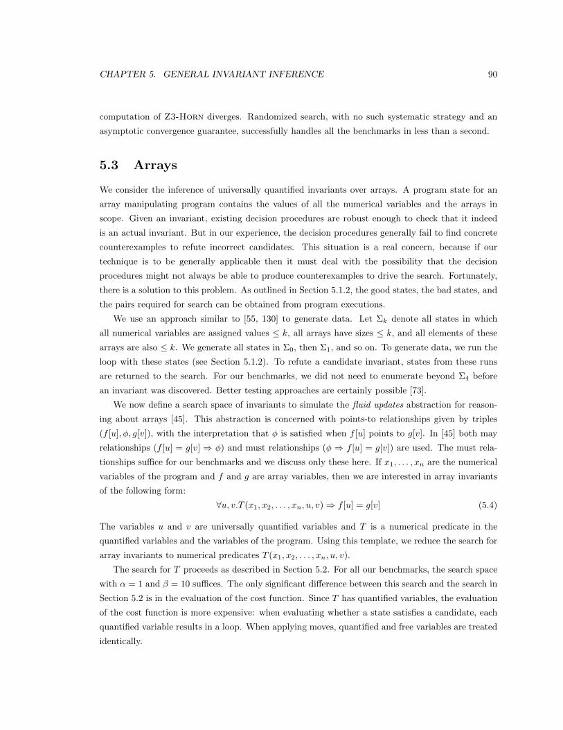
CHAPTER 5. GENERAL INVARIANT INFERENCE 90
computation of Z3-Horn diverges. Randomized search, with no such systematic strategy and an
asymptotic convergence guarantee, successfully handles all the benchmarks in less than a second.
5.3 Arrays
We consider the inference of universally quantified invariants over arrays. A program state for an
array manipulating program contains the values of all the numerical variables and the arrays in
scope. Given an invariant, existing decision procedures are robust enough to check that it indeed
is an actual invariant. But in our experience, the decision procedures generally fail to find concrete
counterexamples to refute incorrect candidates. This situation is a real concern, because if our
technique is to be generally applicable then it must deal with the possibility that the decision
procedures might not always be able to produce counterexamples to drive the search. Fortunately,
there is a solution to this problem. As outlined in Section 5.1.2, the good states, the bad states, and
the pairs required for search can be obtained from program executions.
We use an approach similar to [55, 130] to generate data. Let Σk denote all states in which
all numerical variables are assigned values ≤ k, all arrays have sizes ≤ k, and all elements of these
arrays are also ≤ k. We generate all states in Σ0, then Σ1, and so on. To generate data, we run the
loop with these states (see Section 5.1.2). To refute a candidate invariant, states from these runs
are returned to the search. For our benchmarks, we did not need to enumerate beyond Σ4 before
an invariant was discovered. Better testing approaches are certainly possible [73].
We now define a search space of invariants to simulate the fluid updates abstraction for reason-
ing about arrays [45]. This abstraction is concerned with points-to relationships given by triples
(f [u], φ, g[v]), with the interpretation that φ is satisfied when f [u] points to g[v]. In [45] both may
relationships (f [u] = g[v] ⇒ φ) and must relationships (φ ⇒ f [u] = g[v]) are used. The must rela-
tionships suffice for our benchmarks and we discuss only these here. If x1, . . . , xn are the numerical
variables of the program and f and g are array variables, then we are interested in array invariants
of the following form:
∀u, v.T (x1, x2, . . . , xn, u, v)⇒ f [u] = g[v] (5.4)
The variables u and v are universally quantified variables and T is a numerical predicate in the
quantified variables and the variables of the program. Using this template, we reduce the search for
array invariants to numerical predicates T (x1, x2, . . . , xn, u, v).
The search for T proceeds as described in Section 5.2. For all our benchmarks, the search space
with α = 1 and β = 10 suffices. The only significant difference between this search and the search in
Section 5.2 is in the evaluation of the cost function. Since T has quantified variables, the evaluation
of the cost function is more expensive: when evaluating whether a state satisfies a candidate, each
quantified variable results in a loop. When applying moves, quantified and free variables are treated
identically.

CHAPTER 5. GENERAL INVARIANT INFERENCE 91
Program [45] Z3-H ARMC Dual Pure MCMC Templ
init 0.01 0.06 0.15 0.72 0.06 0.02 0.01init-nc 0.02 0.08 0.48 6.60 0.05 0.15 0.02init-p 0.01 0.03 0.14 2.60 0.01 0.01 0.01init-e 0.04 TO TO TO TO TO TO2darray 0.04 0.18 ? TO 0.02 0.41 0.02copy 0.01 0.04 0.20 1.40 0.87 0.80 0.02copy-p 0.01 0.04 0.21 1.80 0.09 0.13 0.01copy-o 0.04 TO ? 4.50 TO TO 0.50reverse 0.03 0.12 2.28 8.50 TO 3.48 0.03swap 0.12 0.41 3.0 40.60 TO TO 0.21d-swap 0.16 1.37 4.4 TO TO TO 0.51strcpy 0.07 0.05 0.15 0.62 0.01 0.02 0.01strlen 0.02 0.07 0.02 0.20 0.01 0.01 0.01memcpy 0.04 0.20 16.30 0.20 0.02 0.03 0.01find 0.02 0.01 0.08 0.38 2.23 0.30 0.02find-n 0.02 0.01 0.08 0.39 0.07 0.95 0.01append 0.02 0.04 1.76 1.50 TO TO 0.12merge 0.09 0.04 ? 1.50 TO TO 0.41alloc-f 0.02 0.02 0.09 0.69 0.07 0.10 0.01alloc-nf 0.03 0.03 0.13 0.42 0.49 0.14 0.07
Table 5.3: Inference results for array manipulating programs
5.3.1 Evaluation
The principal difference between the evaluation here and in Section 5.2.3 is that there is no feedback
between the search and the decision procedure. We manually wrote harnesses for generating data
and then produced enough data that the search discovers a numerical predicate T that is an invariant
of the array manipulating program. For all benchmarks, at most 150 data elements were sufficient
to obtain an invariant. Just as in Section 5.2.3, we consider three variations of the search for T :
Pure is a pure random walk, MCMC uses the cost function, and Templ restricts the inequalities in T
to a user supplied abstract domain.
We evaluate these randomized search algorithms on the benchmarks of [45] in Table 5.3. The VCs
for these benchmarks were obtained from the repository of the competition on software verification.2
The first column is the name of the program. We have omitted benchmarks with bugs from the
original benchmark set; these bugs are triggered during data generation. The second column shows
the time taken by analyzing these benchmarks using the fluid updates abstraction [45]. Using a
specialized abstract domain leads to a very efficient analysis, but the scope of the analysis is limited
to array manipulating programs that have invariants given by Equation 5.4.
In [19], the authors use templates to reduce the task of inferring universally quantified invariants
2https://svn.sosy-lab.org/software/sv-benchmarks/trunk/clauses/QALIA/

CHAPTER 5. GENERAL INVARIANT INFERENCE 92
for array manipulating programs to numerical invariants and show results using three different back-
ends: Z3-Horn [74], Armc [62], and Duality [100]. These are reproduced verbatim as columns
Z3-H, ARMC, and Dual of Table 5.3. Details about these columns can be found in the original text [19].
Note that the benchmark init-e requires a divisibility constraint that none of these back-ends or
our search algorithms currently support.
The next three columns describe our randomized searches. The time measurements are the total
time to search (with sufficient data) and validate an invariant. We observe that Pure times out
on several benchmarks, which suggests that these problems are harder than those for numerical
invariants. Moreover, whenever the pure random search times out, both Armc and Duality take
more than a second. Hence, there seems to be some correlation between which verification tasks are
difficult for different techniques. Another factor that adversely affects the randomized searches is
that, due to the quantified variables, the evaluation of the cost function is slower than the evaluation
of the cost function for numerical candidates.
The surprising result is that Pure still terminates quickly on the majority of the benchmarks. The
next column shows that MCMC also times out on several benchmarks (these are a subset of benchmarks
on which Pure times out). For these benchmarks, as shown by the last column, just specifying the
abstract domain in which the linear inequalities in the invariant belong suffices to make the search
terminate in under a second. Moreover, Templ is faster than both Armc and Duality on all the
benchmarks of Table 5.3. These results suggest that randomized search is a suitable technique for
inference of universally quantified invariants over arrays and can generate results competitive with
state-of-the-art symbolic inference techniques.
5.4 Strings
Consider the string manipulating program of Figure 5.4 that computes the string (ia)i. To validate
its assertions, the invariants must express facts about the contents of strings, integers, and lengths of
strings; we are unaware of any previous inference technique that can infer such invariants. The string
operations such as length (compute the length of a string), indexof (find the position of a string in
another string), substr (extract a substring between given indices), etc., intermix integers and strings
and pose a challenge for invariant inference. However, the decision procedure Z3-str [153] can decide
i := 0; x := "a";
while(non_det()){ i++; x := "(" + x + ")"; }
assert( x.length == 2*i+1 );
if(i>0) assert( x.contains( "(a)" ) );
Figure 5.4: A program that intermixes strings and integers.

CHAPTER 5. GENERAL INVARIANT INFERENCE 93
Figure 5.4 replace index substring
Pure 342.6 0.01 0.06 0.5MCMC 0.8 0.02 0.06 0.05Z3-str 0.03 TO 114.6 0.01
Table 5.4: Inference results for string manipulating programs. The time taken (in seconds) by purerandom search, by MCMC search, and by Z3-str (for proving the correctness of the invariants) areshown.
formulas over strings and integers. We use Guess-and-Check to construct an invariant inference
procedure from Z3-str.
A program state contains the values of all the numerical and the string variables. The search
space S consists of boolean combinations of predicates that belong to a given bag P of predicates:∨αj=1
(∧βk=1 P
jk
)where P jk ∈ P. The bag P is constructed using the constants and the predicates
occurring in the program. We set α = 5, β = 10, and for Figure 5.4, P has predicates x.contains(y),
y1 = y2, w1i + w2x.length + w3 ≤ 0 where y ∈ {x, “a”, “(”, “)”, “(a)”} and w ∈ [−2 : 2]. A
move replaces a randomly selected P jk with a randomly selected predicate from P. The current
counterexample generation capabilities of Z3-str are unreliable and we generate data using the
process explained in Section 5.3. (At most 25 data elements were sufficient to obtain an invariant.)
For Figure 5.4, randomized search discovers the following invariant and discharges the assertions:
(x = “a” ∧ i = 0
)∨(x.contains(“(a)”) ∧ x.length = 2i+ 1
)Due to the absence of an existing benchmark suite for string-manipulating programs, our evaluation
is limited to a few handwritten examples shown in Table 5.4. The program replace uses replace
(replace the first occurrence of a string with another) in addition to the string operations present in
Figure 5.4. This program checks that repeatedly replacing "a" by "aa" in a loop increases the length
by the number of loop iterations. For this program Z3-str times out in validating the candidate
invariant. We confirmed that the candidate is an invariant manually. The program index uses
indexof in addition to the string operations in replace. This program replaces all occurrences of
one string by another and checks the relationship between the length of the output string and the
number of iterations. Finally, substring uses substr and in this benchmark we prove that a loop
which constructs an http request does not modify the domain name.
An alternative to Guess-and-Check for proving these examples requires designing a new ab-
stract interpretation [36, 37], which entails designing an abstract domain that incorporates both
strings and integers, an abstraction function, a widening operator, and abstract transfer functions
that are precise enough to find disjunctive invariants like the one shown above. Such an alternative
requires significantly greater effort than instantiating Guess-and-Check. In our implementation,
both the proposal mechanism and the eval function, required to instantiate Guess-and-Check, are

CHAPTER 5. GENERAL INVARIANT INFERENCE 94
under 50 lines of C++ each.
5.5 Relations
In this section we define a proposal mechanism to find invariants over relations. We are given a
program with variables x1, x2, . . . , xn and some relations R1, R2, . . . , Rm. A program state is an
evaluation of these variables and these relations. For example, consider the program state i = 1, j =
2, pts = {(1, 2), (2, 1)}, eq = {(1, 1), (2, 2)} where pts is the points-to relation and eq is the equality
relation. In this state i and j point to two heap cells that form a circularly linked list. The invariants
are composed of variables and such relations. The search space consists of predicates F given by
the following grammar:
Predicate F ::=∧θi=1 Fi
Formula F i ::=∧δj=1G
ij
Subformula Gi ::= ∀u1, u2, . . . , ui.TQF Predicate T ::=
∨αk=1
∧βl=1 L
kl
Literal L ::= A | ¬AAtom A ::= R(V1, . . . , Va) a = arity(R)
Argument V ::= x | u | κ
(5.5)
A predicate in the search space is a conjunction of formulas Fi. The subscript of Fi denotes the
number of quantified variables in its subformulas. A subformula is a quantified predicate with its
quantifier free part T expressed in DNF. Each atomic proposition of this DNF formula is a relation
whose arguments can be a variable of the program (x), a quantified variable (u), or some constant
(κ) like null. We focus our attention on universally quantified predicates. Predicates with existential
quantifiers and arbitrary alternations can also be incorporated easily in the search, but validating
such candidates is much harder [138]. The variables in scope of a relation in a predicate are the
program variables and the quantified variables in the associated subformulas.
Next we define the moves of our proposal mechanism. We select a move uniformly at random
from the list below and apply it to the current candidate C. As usual, we write “at random” to
mean “uniformly at random”.
1. Variable move: Select an atom of C at random. Next, select one of the arguments and replace
it with an argument selected at random from the variables in scope and the constants.
2. Relation move: Select an atom of C at random and replace its relation with a relation selected
at random from the set of relations of the same arity. The arguments are unaffected.
3. Atom move: Select an atom of C at random and replace its relation with a relation selected at
random from all available relations. Perform variable moves to fill the arguments of the new

CHAPTER 5. GENERAL INVARIANT INFERENCE 95
relation.
4. Flip polarity: Negate a literal selected at random from the literals of C.
5. Literal move: Perform an atom move and flip polarity.
These moves are ergodic: using atom moves and flipping polarity it is possible to transform any
candidate C1 into any other candidate C2. Moreover, these moves are symmetric and hence the
proposal mechanism satisfies symmetry.
Next, we evaluate the MCMC algorithm in Figure 5.1 with this proposal mechanism and the cost
function of Equation 5.3. We also evaluate a pure variation in which all moves are accepted. We do
not evaluate a “template” variation as the relations can be seen as templates and it is unclear what
additional template restrictions could be added.
5.5.1 Lists
We use the relational proposal mechanism to prove functional properties of linked list manipulating
programs. The heap is composed of cells and each cell either contains null or the address of another
cell. The reachability relation n∗(i, j) holds if the cell pointed to by j can be reached from i using
zero or more pointer dereferences. While writing post-conditions to express functional properties,
it is useful to talk about the reachability relation that holds before the program begins execution.
We denote this binary relation by n∗. Using these relations, the predicates in our search space are
universally quantified formulas over these reachability relations for linked list manipulating programs.
A recently published decision procedure is complete for such candidates via a reduction of such
formulas to boolean satisfiability [76]. It takes a program annotated with invariants as input and
checks the assertions. We use this decision procedure as our validator and randomized search to
find invariants for some standard singly linked list manipulating programs. The evaluation of [76]
shows that it can handle relations and hence can validate a variety of programs that have been
hand-annotated with invariants. During our evaluation of various verification tasks, we observed
that such decision procedures for advanced logics are not able to accept all formulas in their input
language. Hence, sometimes we must perform some equality-preserving simplifications on the candi-
date invariants our search discovers. Currently we perform this step manually when necessary, but
the simplifications could be automated.
5.5.2 Evaluation
For defining the search space using Equation 5.5 we set α = β = δ = 5 and θ = 2, which is sufficient
to express the invariants for all of our benchmarks. Our evaluation results on the benchmarks of [76]
are in Table 5.5. The first column lists the programs, all of which perform basic manipulations of
singly linked lists. The program delete removes a specific element of the list, deleteall deletes
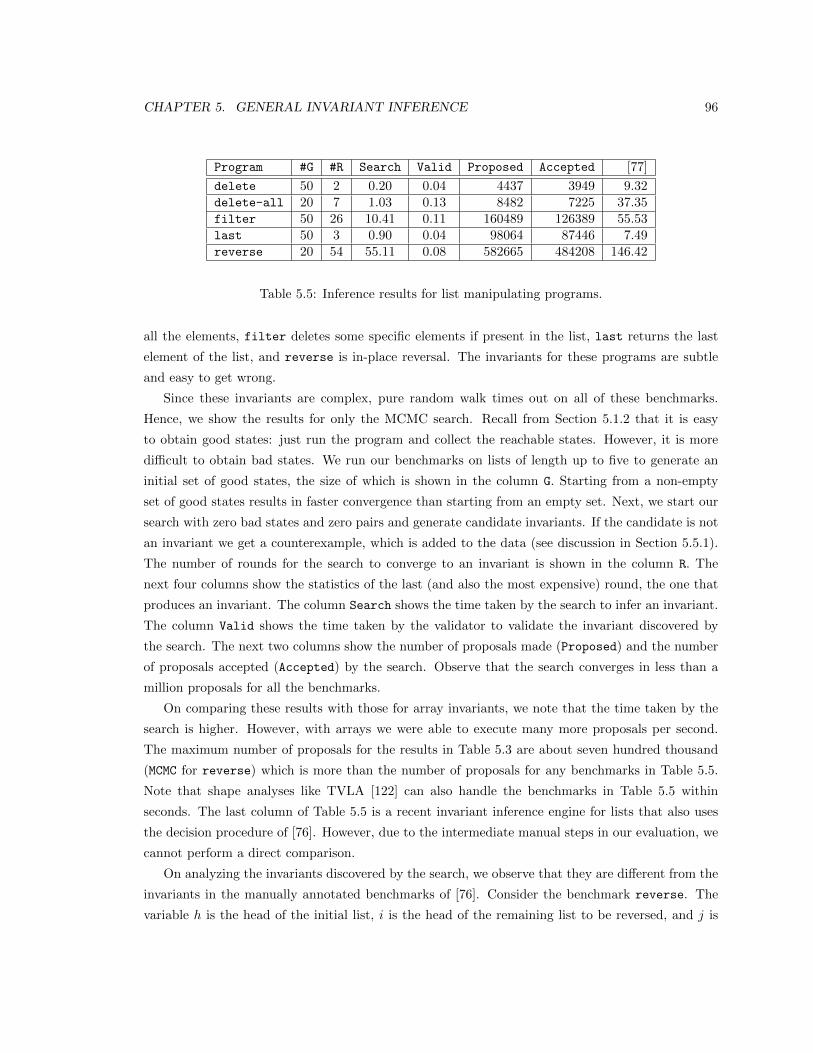
CHAPTER 5. GENERAL INVARIANT INFERENCE 96
Program #G #R Search Valid Proposed Accepted [77]
delete 50 2 0.20 0.04 4437 3949 9.32delete-all 20 7 1.03 0.13 8482 7225 37.35filter 50 26 10.41 0.11 160489 126389 55.53last 50 3 0.90 0.04 98064 87446 7.49reverse 20 54 55.11 0.08 582665 484208 146.42
Table 5.5: Inference results for list manipulating programs.
all the elements, filter deletes some specific elements if present in the list, last returns the last
element of the list, and reverse is in-place reversal. The invariants for these programs are subtle
and easy to get wrong.
Since these invariants are complex, pure random walk times out on all of these benchmarks.
Hence, we show the results for only the MCMC search. Recall from Section 5.1.2 that it is easy
to obtain good states: just run the program and collect the reachable states. However, it is more
difficult to obtain bad states. We run our benchmarks on lists of length up to five to generate an
initial set of good states, the size of which is shown in the column G. Starting from a non-empty
set of good states results in faster convergence than starting from an empty set. Next, we start our
search with zero bad states and zero pairs and generate candidate invariants. If the candidate is not
an invariant we get a counterexample, which is added to the data (see discussion in Section 5.5.1).
The number of rounds for the search to converge to an invariant is shown in the column R. The
next four columns show the statistics of the last (and also the most expensive) round, the one that
produces an invariant. The column Search shows the time taken by the search to infer an invariant.
The column Valid shows the time taken by the validator to validate the invariant discovered by
the search. The next two columns show the number of proposals made (Proposed) and the number
of proposals accepted (Accepted) by the search. Observe that the search converges in less than a
million proposals for all the benchmarks.
On comparing these results with those for array invariants, we note that the time taken by the
search is higher. However, with arrays we were able to execute many more proposals per second.
The maximum number of proposals for the results in Table 5.3 are about seven hundred thousand
(MCMC for reverse) which is more than the number of proposals for any benchmarks in Table 5.5.
Note that shape analyses like TVLA [122] can also handle the benchmarks in Table 5.5 within
seconds. The last column of Table 5.5 is a recent invariant inference engine for lists that also uses
the decision procedure of [76]. However, due to the intermediate manual steps in our evaluation, we
cannot perform a direct comparison.
On analyzing the invariants discovered by the search, we observe that they are different from the
invariants in the manually annotated benchmarks of [76]. Consider the benchmark reverse. The
variable h is the head of the initial list, i is the head of the remaining list to be reversed, and j is
CHAPTER 5. GENERAL INVARIANT INFERENCE 97
the head of the reversed list. The pre-condition is that the heap contains only the linked list and
nothing else. The program is as follows:
i = h; j = null; while (i != null) { k=*i; *i=j; j=i; i=k; }
For reverse the search discovers the following invariant:
∀u(u 6= null ⇒ (n∗(i, u) ∨ n∗(j, u)))
∀u, v(n∗(u, v)⇒ (¬ n∗(i, u) ∧ n∗(v, u) ∨ n∗(u, v) ∧ ¬ n∗(u, j)))
The decision procedure of [76] is able to validate this invariant and uses it to show that reverse
correctly reverses a linked list. Note that this invariant is more succinct and difficult to comprehend
than the invariant written by hand in [76]:
∀u(u 6= null ⇒ (n∗(i, u)⇔ ¬n∗(j, u)))
∀u, v(n∗(i, u)⇒ (n∗(u, v)⇔ n∗(u, v)))
∀u, v(n∗(j, u)⇒ (n∗(u, v)⇔ n∗(v, u)))
This easier to understand invariant says that every node is either in the partially reversed list or
the to be reversed list. In the to be reversed list, the reachability relation is unchanged and in the
partially reversed list the reachability relation is reverse of the initial.
Since the decision procedure of [76] is complete, it is able to consume and verify any unusual
invariants that the search produces. Generally the decision procedures for more advanced data
structures are not so robust that they can consume arbitrary candidates. Often, one needs to write
the invariants with care and might even need to provide additional axioms or lemmas to verify
more advanced data structure manipulating programs [116]. Once the state of the art of these
decision procedures improve, we can apply randomized search for these programs too. We do not
need a complete decision procedure as we can generate data by running the programs, just as we
do for arrays and strings. But the decision procedure should be robust enough to handle arbitrary
candidate invariants automatically.
5.6 Related Work
The goal of this chapter is a framework to obtain inference engines from decision procedures. Guess-
and-Check is parametrized by the language of possible invariants. This characteristic is similar
to TVLA [122], which is a parametric shape analysis. TVLA requires specialized heuristics (focus,
coerce, etc.) to maintain precision. We do not require these heuristics and this generality aids us in
obtaining inference procedures for verification tasks beyond shape analysis. Guess-and-Check is a
template-based analysis that does not use decision procedures to instantiate the templates and limits
their use to checking an annotated program. We do not rely on decision procedures to compute a
CHAPTER 5. GENERAL INVARIANT INFERENCE 98
predicate cover [69], or for fixpoint iterations [54, 137], or on Farkas’ lemma [17, 35, 68, 71]. Hence,
Guess-and-Check is applicable to various decision procedures, including the incomplete procedures
(Section 5.3 and Section 5.4).
Most techniques for invariant inference are symbolic analyses that trade generality for effective
techniques in specific domains [16, 26, 47, 71, 77, 84]. We are not aware of any symbolic inference
technique that has been successfully demonstrated to infer invariants for the various types of pro-
grams that we consider (numeric, array, string, and list). We have shown that invariant search using
concrete data and general search procedures such as Metropolis Hastings has the potential to be a
general solution to obtain inference procedures from checking procedures. We discuss the related
techniques that learn invariants from concrete data and compare them with randomized search.
Concrete states can help maintain precision by aiding the computation of the best abstract trans-
formers [118]. However, this approach suffers from irrecoverable imprecision as it relies on widening
heuristics for termination. In contrast, randomized search can always recover from excessive under
or over approximations, but only provides an asymptotic guarantee of termination if an invariant
exists. The inference algorithm for numerical invariants described in [56] uses decision procedures
to search for candidate invariants. It is not clear whether decision procedures can effectively search
for good candidates that satisfy data over quantified domains. There are several automata-based
approaches for learning invariants [33, 55, 56]. It is unclear whether automata can express numerical
invariants. Domain-specific search procedures like these seem unsuitable for a general framework for
obtaining inference procedures from checking procedures.
Algorithmic learning [83, 88] based approaches also iteratively invoke search and validate phases.
They use a CDNF learning algorithm that requires membership queries (is a conjunction of atomic
predicates contained in the invariant) and equivalence queries (is the candidate an invariant). Since
the invariant is unknown, the membership queries are resolved heuristically. In contrast, Guess-
and-Check does not require membership queries. Other techniques that use concrete data to guide
verification include [4, 64, 67, 104].
We are unaware of the any previous work that uses Metropolis Hastings sampler for invariant
inference. In a related work, [66] uses Gibbs sampling for inference of numerical invariants. However,
the inference works directly on the program (it computes pre-conditions and post-conditions) as
opposed to concrete data. Handling programs with pointers and arrays is left as an open problem
by [66].
We use efficiency to guide the choice of parameters for randomized search. E.g., in our evalua-
tions, we set γ in Figure 5.1 to loge 2. Systematic approaches described in [132] can also be used
for setting such parameters.
MCMC based search has been found to be useful in superoptimization [126], where the goal is to
infer an assembly program that satisfies some concrete input/output examples. MCMC search has
also been used in program testing to achieve better coverage [123]. A randomized scheduler is used

CHAPTER 5. GENERAL INVARIANT INFERENCE 99
to find concurrency bugs in [23].

Chapter 6
Conclusion
In this thesis, we have discussed loop invariant inference techniques that combine static analysis and
machine learning. We break down the problem of invariant inference into two phases. In the guess
phase, the loop is executed on a few inputs and the observed program states are logged. These logs
constitute our data. Subsequently, a learner guesses a candidate invariant from the data. In the
check phase, a static analysis proves whether the candidate invariant is an actual invariant or not.
In the former case, the inference succeeds. In the latter case, we repeat the process with additional
data.
This Guess-and-Check approach helps us achieve new results. Chapter 2 describes a sound
and relatively complete algorithm for inference of algebraic invariants that finds correct invariants
(if the SMT solver can answer all queries correctly) and the inferred invariant is the best possible in
the given class. In contrast, all previous tools for inferring algebraic equality invariants unsoundly
approximate integral program variables by real-valued variables. Chapter 3 describes DDEC, the
first equivalence checker for x86. The key idea that makes DDEC effective in practice, and even
simply feasible to build, is that the process of guessing a simulation relation is constructed not via
static code analyses, but by using data collected from tests. Chapter 4 presents the first invariant
inference technique that does not place any ad-hoc restriction on the number of disjunctions while
also guaranteeing that invariants are of bounded size. Naive approaches tend to generate a very
large or even an unbounded number of disjunctions, leading to non-terminating analyses. Therefore,
to ensure tractability, all previous analyses use a user-provided or an ad-hoc bound on the number of
disjunctions. Chapter 5 presents an approach to infer arbitrary invariants. Instantiating the Guess-
and-Check approach with MCMC samplers as learners and suitable SMT solvers yields inference
engines for many classes, including those for which invariant inference techniques were previously
unknown.
A common theme of these chapters is the observation that the decomposition of invariant in-
ference into two phases substantially simplifies the architecture of a verifier and leads to simpler
100

CHAPTER 6. CONCLUSION 101
implementations. The learners are just data crunching algorithms that are easy to implement. For
checking, we use off-the-shelf SMT solvers and take advantage of recent advances in automatic
theorem proving.
Although this thesis focuses on loop invariants, it is possible to leverage the data-driven tech-
niques for many other inference tasks. For example, consider the problem of program termination.
Termination proofs are based on inferring variants or ranking functions. We have used data to infer
ranking functions in [110]. Data has also assisted us in proving race freedom and deadlock freedom
of aggressively optimized GPU programs [128]. We explored connections between program analyses
and statistical machine learning in [132], and these connections helped significantly improve the
performance of an industrial strength device-driver verifier. We believe that data-driven techniques
can significantly enhance the state of the art in many other verification tasks.
Since data-driven techniques are very different from the symbolic techniques routinely used in
verification, the Guess-and-Check based inference engines have different strengths and weaknesses
compared to traditional static analyses. Intuitively, a purely static analysis is governed by a proof
goal and tries to infer logic formulas that would help the proof go through. In contrast, the learner
observes concrete states and mines patterns that are apparent in the data and produces them as
candidate invariants. The learners studied in machine learning are often guided by Occam’s razor
and aim to generate the simplest hypotheses that explain the data. A Guess-and-Check approach
succeeds if the simple patterns are sufficient for the proof. Since programmers/compilers reason
about the correctness of the code they generate, in many cases, the invariants are indeed simple
and the candidates guessed via learning are useful. However, some verification tasks can require
invariants that are larger than the programs themselves and a purely static analysis can perform
better than Guess-and-Check for such cases.
There are several domains where the data-driven techniques described in this thesis are currently
inapplicable, such as verification of models or abstract specifications. Such models are usually not
executable, and data generation fails. In verification using interactive theorem provers, it is typical to
construct a proof and an implementation together. Therefore, unless the proof has been completed,
an executable program is not available, and data cannot be generated. Rich symbolic techniques for
data generation can help alleviate some of these concerns. Finally, the invariants considered in this
thesis can be inferred by simple learners and consumed by SMT solvers. More expressive invariants
pose a challenge for both the existing learners and the existing checkers; these would require new
techniques beyond this thesis.

Bibliography
[1] Behzad Akbarpour and Lawrence C. Paulson. MetiTarski: An automatic theorem prover for
real-valued special functions. J. Autom. Reasoning, 44(3):175–205, 2010.
[2] Aws Albarghouthi, Arie Gurfinkel, and Marsha Chechik. Craig interpretation. In Static
Analysis - 19th International Symposium, SAS 2012, Deauville, France, September 11-13,
2012. Proceedings, pages 300–316, 2012.
[3] Rajeev Alur, Rastislav Bodık, Garvit Juniwal, Milo M. K. Martin, Mukund Raghothaman,
Sanjit A. Seshia, Rishabh Singh, Armando Solar-Lezama, Emina Torlak, and Abhishek Udupa.
Syntax-guided synthesis. In Formal Methods in Computer-Aided Design, FMCAD 2013, Port-
land, OR, USA, October 20-23, 2013, pages 1–8, 2013.
[4] Gianluca Amato, Maurizio Parton, and Francesca Scozzari. Discovering invariants via simple
component analysis. J. Symb. Comput., 47(12):1533–1560, 2012.
[5] Christophe Andrieu, Nando De Freitas, Arnaud Doucet, and Michael I Jordan. An introduction
to MCMC for machine learning. Machine learning, 50(1-2):5–43, 2003.
[6] Tamarah Arons, Elad Elster, Limor Fix, Sela Mador-Haim, Michael Mishaeli, Jonathan Shalev,
Eli Singerman, Andreas Tiemeyer, Moshe Y. Vardi, and Lenore D. Zuck. Formal verification
of backward compatibility of microcode. In Computer Aided Verification, 17th International
Conference, CAV 2005, Edinburgh, Scotland, UK, July 6-10, 2005, Proceedings, pages 185–
198, 2005.
[7] David F. Bacon, Susan L. Graham, and Oliver J. Sharp. Compiler transformations for high-
performance computing. ACM Comput. Surv., 26(4):345–420, 1994.
[8] Roberto Bagnara, Patricia M. Hill, and Enea Zaffanella. Widening operators for powerset
domains. STTT, 9(3-4):413–414, 2007.
[9] Roberto Bagnara, Enric Rodrıguez-Carbonell, and Enea Zaffanella. Generation of basic semi-
algebraic invariants using convex polyhedra. In Static Analysis, 12th International Symposium,
SAS 2005, London, UK, September 7-9, 2005, Proceedings, pages 19–34, 2005.
102

BIBLIOGRAPHY 103
[10] Gogul Balakrishnan and Thomas W. Reps. WYSINWYX: What you see is not what you
eXecute. ACM Trans. Program. Lang. Syst., 32(6), 2010.
[11] Thomas Ball, Brian Hackett, Shuvendu K. Lahiri, Shaz Qadeer, and Julien Vanegue. Towards
scalable modular checking of user-defined properties. In Verified Software: Theories, Tools,
Experiments, Third International Conference, VSTTE 2010, Edinburgh, UK, August 16-19,
2010. Proceedings, pages 1–24, 2010.
[12] Thomas Ball and Sriram K. Rajamani. The SLAM toolkit. In Computer Aided Verification,
13th International Conference, CAV 2001, Paris, France, July 18-22, 2001, Proceedings, pages
260–264, 2001.
[13] Michael Barnett, Bor-Yuh Evan Chang, Robert DeLine, Bart Jacobs, and K. Rustan M.
Leino. Boogie: A modular reusable verifier for object-oriented programs. In Formal Methods
for Components and Objects, 4th International Symposium, FMCO 2005, Amsterdam, The
Netherlands, November 1-4, 2005, Revised Lectures, pages 364–387, 2005.
[14] Bonnie Berger, John Rompel, and Peter W. Shor. Efficient NC algorithms for set cover with
applications to learning and geometry. J. Comput. Syst. Sci., 49(3):454–477, 1994.
[15] Dirk Beyer. Competition on Software Verification (SV-COMP) benchmarks. https://svn. sosy-
lab.org/software/sv-benchmarks/tags/svcomp13/loops/.
[16] Dirk Beyer, Thomas A. Henzinger, Ranjit Jhala, and Rupak Majumdar. The software model
checker Blast. STTT, 9(5-6):505–525, 2007.
[17] Dirk Beyer, Thomas A. Henzinger, Rupak Majumdar, and Andrey Rybalchenko. Invariant
synthesis for combined theories. In Verification, Model Checking, and Abstract Interpretation,
8th International Conference, VMCAI 2007, Nice, France, January 14-16, 2007, Proceedings,
pages 378–394, 2007.
[18] Dirk Beyer, Thomas A. Henzinger, Rupak Majumdar, and Andrey Rybalchenko. Path in-
variants. In Proceedings of the ACM SIGPLAN 2007 Conference on Programming Language
Design and Implementation, San Diego, California, USA, June 10-13, 2007, pages 300–309,
2007.
[19] Nikolaj Bjørner, Kenneth L. McMillan, and Andrey Rybalchenko. On solving universally
quantified Horn clauses. In Static Analysis - 20th International Symposium, SAS 2013, Seattle,
WA, USA, June 20-22, 2013. Proceedings, pages 105–125, 2013.
[20] Anselm Blumer, Andrzej Ehrenfeucht, David Haussler, and Manfred K. Warmuth. Learnability
and the Vapnik-Chervonenkis dimension. J. ACM, 36(4):929–965, 1989.

BIBLIOGRAPHY 104
[21] Herve Bronnimann and Michael T. Goodrich. Almost optimal set covers in finite VC-
dimension. Discrete & Computational Geometry, 14(4):463–479, 1995.
[22] Nader H. Bshouty, Sally A. Goldman, H. David Mathias, Subhash Suri, and Hisao Tamaki.
Noise-tolerant distribution-free learning of general geometric concepts. In Proceedings of the
Twenty-Eighth Annual ACM Symposium on the Theory of Computing, Philadelphia, Pennsyl-
vania, USA, May 22-24, 1996, pages 151–160, 1996.
[23] Sebastian Burckhardt, Pravesh Kothari, Madanlal Musuvathi, and Santosh Nagarakatte. A
randomized scheduler with probabilistic guarantees of finding bugs. In Proceedings of the 15th
International Conference on Architectural Support for Programming Languages and Operating
Systems, ASPLOS 2010, Pittsburgh, Pennsylvania, USA, March 13-17, 2010, pages 167–178,
2010.
[24] Jacob Burnim, Nicholas Jalbert, Christos Stergiou, and Koushik Sen. Looper: Lightweight
detection of infinite loops at runtime. In ASE 2009, 24th IEEE/ACM International Conference
on Automated Software Engineering, Auckland, New Zealand, November 16-20, 2009, pages
161–169, 2009.
[25] David Cachera, Thomas P. Jensen, Arnaud Jobin, and Florent Kirchner. Inference of polyno-
mial invariants for imperative programs: A farewell to Grobner bases. In Static Analysis - 19th
International Symposium, SAS 2012, Deauville, France, September 11-13, 2012. Proceedings,
pages 58–74, 2012.
[26] Cristiano Calcagno, Dino Distefano, Peter W. O’Hearn, and Hongseok Yang. Compositional
shape analysis by means of bi-abduction. In Proceedings of the 36th ACM SIGPLAN-SIGACT
Symposium on Principles of Programming Languages, POPL 2009, Savannah, GA, USA, Jan-
uary 21-23, 2009, pages 289–300, 2009.
[27] Zhuliang Chen and Arne Storjohann. A BLAS based C library for exact linear algebra on
integer matrices. In Symbolic and Algebraic Computation, International Symposium ISSAC
2005, Beijing, China, July 24-27, 2005, Proceedings, pages 92–99, 2005.
[28] Siddhartha Chib and Edward Greenberg. Understanding the Metropolis-Hastings algorithm.
The American Statistician, 49(4):327–335, 1995.
[29] Chris Lattner and Vikram Adve. The LLVM Instruction Set and Compilation Strategy. Tech.
Report UIUCDCS-R-2002-2292, CS Dept., Univ. of Illinois at Urbana-Champaign, Aug 2002.
[30] V Chvatal. A greedy heuristic for the set-covering problem. Mathematics of Operations Re-
search, 4(3):233–235, 1979.

BIBLIOGRAPHY 105
[31] Robert Clariso and Jordi Cortadella. The octahedron abstract domain. In Static Analysis,
11th International Symposium, SAS 2004, Verona, Italy, August 26-28, 2004, Proceedings,
pages 312–327, 2004.
[32] Edmund M. Clarke, Orna Grumberg, Somesh Jha, Yuan Lu, and Helmut Veith.
Counterexample-guided abstraction refinement. In Computer Aided Verification, 12th In-
ternational Conference, CAV 2000, Chicago, IL, USA, July 15-19, 2000, Proceedings, pages
154–169, 2000.
[33] Jamieson M. Cobleigh, Dimitra Giannakopoulou, and Corina S. Pasareanu. Learning assump-
tions for compositional verification. In Tools and Algorithms for the Construction and Analysis
of Systems, 9th International Conference, TACAS 2003, Held as Part of the Joint European
Conferences on Theory and Practice of Software, ETAPS 2003, Warsaw, Poland, April 7-11,
2003, Proceedings, pages 331–346, 2003.
[34] Michael Colon. Approximating the algebraic relational semantics of imperative programs. In
Static Analysis, 11th International Symposium, SAS 2004, Verona, Italy, August 26-28, 2004,
Proceedings, pages 296–311, 2004.
[35] Michael Colon, Sriram Sankaranarayanan, and Henny Sipma. Linear invariant generation using
non-linear constraint solving. In Computer Aided Verification, 15th International Conference,
CAV 2003, Boulder, CO, USA, July 8-12, 2003, Proceedings, pages 420–432, 2003.
[36] Giulia Costantini, Pietro Ferrara, and Agostino Cortesi. Static analysis of string values. In For-
mal Methods and Software Engineering - 13th International Conference on Formal Engineering
Methods, ICFEM 2011, Durham, UK, October 26-28, 2011. Proceedings, pages 505–521, 2011.
[37] Patrick Cousot and Radhia Cousot. Abstract interpretation: A unified lattice model for static
analysis of programs by construction or approximation of fixpoints. In Conference Record of the
Fourth ACM Symposium on Principles of Programming Languages, Los Angeles, California,
USA, January 1977, pages 238–252, 1977.
[38] Patrick Cousot and Radhia Cousot. Systematic design of program analysis frameworks. In
Conference Record of the Sixth Annual ACM Symposium on Principles of Programming Lan-
guages, San Antonio, Texas, USA, January 1979, pages 269–282, 1979.
[39] Patrick Cousot, Radhia Cousot, Jerome Feret, Laurent Mauborgne, Antoine Mine, David
Monniaux, and Xavier Rival. The ASTREE analyzer. In Programming Languages and Systems,
14th European Symposium on Programming, ESOP 2005, Held as Part of the Joint European
Conferences on Theory and Practice of Software, ETAPS 2005, Edinburgh, UK, April 4-8,
2005, Proceedings, pages 21–30, 2005.

BIBLIOGRAPHY 106
[40] Patrick Cousot and Nicolas Halbwachs. Automatic discovery of linear restraints among vari-
ables of a program. In Conference Record of the Fifth Annual ACM Symposium on Principles
of Programming Languages, Tucson, Arizona, USA, January 1978, pages 84–96, 1978.
[41] David A. Cox, John Little, and Donal O’Shea. Ideals, Varieties, and Algorithms - An In-
troduction to Computational Algebraic Geometry and Commutative Algebra. Undergraduate
texts in mathematics. Springer, 1997.
[42] David W. Currie, Alan J. Hu, and Sreeranga P. Rajan. Automatic formal verification of DSP
software. In Proceedings of the 37th Conference on Design Automation, Los Angeles, CA,
USA, June 5-9, 2000. ACM, 2000, pages 130–135, 2000.
[43] Leonardo Mendonca de Moura and Nikolaj Bjørner. Z3: an efficient SMT solver. In Tools
and Algorithms for the Construction and Analysis of Systems, 14th International Conference,
TACAS 2008, Held as Part of the Joint European Conferences on Theory and Practice of
Software, ETAPS 2008, Budapest, Hungary, March 29-April 6, 2008. Proceedings, pages 337–
340, 2008.
[44] Edsger W. Dijkstra. A Discipline of Programming. Prentice-Hall, 1976.
[45] Isil Dillig, Thomas Dillig, and Alex Aiken. Fluid updates: Beyond strong vs. weak updates.
In Programming Languages and Systems, 19th European Symposium on Programming, ESOP
2010, Held as Part of the Joint European Conferences on Theory and Practice of Software,
ETAPS 2010, Paphos, Cyprus, March 20-28, 2010. Proceedings, pages 246–266, 2010.
[46] Isil Dillig, Thomas Dillig, and Alex Aiken. Small formulas for large programs: On-line con-
straint simplification in scalable static analysis. In Static Analysis - 17th International Sym-
posium, SAS 2010, Perpignan, France, September 14-16, 2010. Proceedings, pages 236–252,
2010.
[47] Isil Dillig, Thomas Dillig, Boyang Li, and Kenneth L. McMillan. Inductive invariant generation
via abductive inference. In Proceedings of the 2013 ACM SIGPLAN International Conference
on Object Oriented Programming Systems Languages & Applications, OOPSLA 2013, part of
SPLASH 2013, Indianapolis, IN, USA, October 26-31, 2013, pages 443–456, 2013.
[48] Matt Elder, Junghee Lim, Tushar Sharma, Tycho Andersen, and Thomas W. Reps. Abstract
domains of affine relations. ACM Trans. Program. Lang. Syst., 36(4):11:1–11:73, 2014.
[49] Michael D. Ernst, Jeff H. Perkins, Philip J. Guo, Stephen McCamant, Carlos Pacheco,
Matthew S. Tschantz, and Chen Xiao. The daikon system for dynamic detection of likely
invariants. Sci. Comput. Program., 69(1-3):35–45, 2007.

BIBLIOGRAPHY 107
[50] Manuel Fahndrich and Francesco Logozzo. Static contract checking with abstract interpreta-
tion. In Formal Verification of Object-Oriented Software - International Conference, FoVeOOS
2010, Paris, France, June 28-30, 2010, Revised Selected Papers, pages 10–30, 2010.
[51] Xiushan Feng and Alan J. Hu. Automatic formal verification for scheduled VLIW code. In
Proceedings of the 2002 Joint Conference on Languages, Compilers, and Tools for Embedded
Systems & Software and Compilers for Embedded Systems (LCTES’02-SCOPES’02), Berlin,
Germany, 19-21 June 2002, pages 85–92, 2002.
[52] Xiushan Feng and Alan J. Hu. Cutpoints for formal equivalence verification of embedded
software. In EMSOFT 2005, September 18-22, 2005, Jersey City, NJ, USA, 5th ACM Inter-
national Conference On Embedded Software, Proceedings, pages 307–316, 2005.
[53] Gilberto File and Francesco Ranzato. Improving abstract interpretations by systematic lifting
to the powerset. In Logic Programming, Proceedings of the 1994 International Symposium,
Ithaca, New York, USA, November 13-17, 1994, pages 655–669, 1994.
[54] Cormac Flanagan and K. Rustan M. Leino. Houdini, an annotation assistant for esc/java. In
FME 2001: Formal Methods for Increasing Software Productivity, International Symposium
of Formal Methods Europe, Berlin, Germany, March 12-16, 2001, Proceedings, pages 500–517,
2001.
[55] Pranav Garg, Christof Loding, P. Madhusudan, and Daniel Neider. Learning universally quan-
tified invariants of linear data structures. In Computer Aided Verification - 25th International
Conference, CAV 2013, Saint Petersburg, Russia, July 13-19, 2013. Proceedings, pages 813–
829, 2013.
[56] Pranav Garg, Christof Loding, P. Madhusudan, and Daniel Neider. ICE: A robust framework
for learning invariants. In Computer Aided Verification - 26th International Conference, CAV
2014, Held as Part of the Vienna Summer of Logic, VSL 2014, Vienna, Austria, July 18-22,
2014. Proceedings, pages 69–87, 2014.
[57] Khalil Ghorbal, Franjo Ivancic, Gogul Balakrishnan, Naoto Maeda, and Aarti Gupta. Donut
domains: Efficient non-convex domains for abstract interpretation. In Verification, Model
Checking, and Abstract Interpretation - 13th International Conference, VMCAI 2012, Philadel-
phia, PA, USA, January 22-24, 2012. Proceedings, pages 235–250, 2012.
[58] Patrice Godefroid and Ankur Taly. Automated synthesis of symbolic instruction encodings
from I/O samples. In ACM SIGPLAN Conference on Programming Language Design and
Implementation, PLDI ’12, Beijing, China - June 11 - 16, 2012, pages 441–452, 2012.
BIBLIOGRAPHY 108
[59] Benny Godlin and Ofer Strichman. Regression verification. In Proceedings of the 46th Design
Automation Conference, DAC 2009, San Francisco, CA, USA, July 26-31, 2009, pages 466–
471, 2009.
[60] Benjamin Goldberg, Lenore D. Zuck, and Clark W. Barrett. Into the loops: Practical issues in
translation validation for optimizing compilers. Electr. Notes Theor. Comput. Sci., 132(1):53–
71, 2005.
[61] Denis Gopan and Thomas W. Reps. Guided static analysis. In Static Analysis, 14th Interna-
tional Symposium, SAS 2007, Kongens Lyngby, Denmark, August 22-24, 2007, Proceedings,
pages 349–365, 2007.
[62] Sergey Grebenshchikov, Nuno P. Lopes, Corneliu Popeea, and Andrey Rybalchenko. Synthe-
sizing software verifiers from proof rules. In ACM SIGPLAN Conference on Programming
Language Design and Implementation, PLDI ’12, Beijing, China - June 11 - 16, 2012, pages
405–416, 2012.
[63] Bhargav S. Gulavani, Supratik Chakraborty, Aditya V. Nori, and Sriram K. Rajamani. Auto-
matically refining abstract interpretations. In Tools and Algorithms for the Construction and
Analysis of Systems, 14th International Conference, TACAS 2008, Held as Part of the Joint
European Conferences on Theory and Practice of Software, ETAPS 2008, Budapest, Hungary,
March 29-April 6, 2008. Proceedings, pages 443–458, 2008.
[64] Bhargav S. Gulavani, Thomas A. Henzinger, Yamini Kannan, Aditya V. Nori, and Sriram K.
Rajamani. SYNERGY: a new algorithm for property checking. In Proceedings of the 14th
ACM SIGSOFT International Symposium on Foundations of Software Engineering, FSE 2006,
Portland, Oregon, USA, November 5-11, 2006, pages 117–127, 2006.
[65] Sumit Gulwani. Program analysis using random interpretation. In Ph.D. Dissertation, UC-
Berkeley, 2005.
[66] Sumit Gulwani and Nebojsa Jojic. Program verification as probabilistic inference. In Pro-
ceedings of the 34th ACM SIGPLAN-SIGACT Symposium on Principles of Programming Lan-
guages, POPL 2007, Nice, France, January 17-19, 2007, pages 277–289, 2007.
[67] Sumit Gulwani and George C. Necula. Discovering affine equalities using random interpre-
tation. In Conference Record of POPL 2003: The 30th SIGPLAN-SIGACT Symposium on
Principles of Programming Languages, New Orleans, Louisisana, USA, January 15-17, 2003,
pages 74–84, 2003.
[68] Sumit Gulwani, Saurabh Srivastava, and Ramarathnam Venkatesan. Program analysis as
constraint solving. In Proceedings of the ACM SIGPLAN 2008 Conference on Programming

BIBLIOGRAPHY 109
Language Design and Implementation, Tucson, AZ, USA, June 7-13, 2008, pages 281–292,
2008.
[69] Sumit Gulwani, Saurabh Srivastava, and Ramarathnam Venkatesan. Constraint-based in-
variant inference over predicate abstraction. In Verification, Model Checking, and Abstract
Interpretation, 10th International Conference, VMCAI 2009, Savannah, GA, USA, January
18-20, 2009. Proceedings, pages 120–135, 2009.
[70] Ashutosh Gupta, Thomas A. Henzinger, Rupak Majumdar, Andrey Rybalchenko, and Ru-
Gang Xu. Proving non-termination. In Proceedings of the 35th ACM SIGPLAN-SIGACT
Symposium on Principles of Programming Languages, POPL 2008, San Francisco, California,
USA, January 7-12, 2008, pages 147–158, 2008.
[71] Ashutosh Gupta, Rupak Majumdar, and Andrey Rybalchenko. From tests to proofs. In Tools
and Algorithms for the Construction and Analysis of Systems, 15th International Conference,
TACAS 2009, Held as Part of the Joint European Conferences on Theory and Practice of
Software, ETAPS 2009, York, UK, March 22-29, 2009. Proceedings, pages 262–276, 2009.
[72] Neelam Gupta and Zachary V. Heidepriem. A new structural coverage criterion for dynamic
detection of program invariants. In 18th IEEE International Conference on Automated Soft-
ware Engineering (ASE 2003), 6-10 October 2003, Montreal, Canada, pages 49–59, 2003.
[73] Michael Harder, Jeff Mellen, and Michael D. Ernst. Improving test suites via operational
abstraction. In Proceedings of the 25th International Conference on Software Engineering,
May 3-10, 2003, Portland, Oregon, USA, pages 60–73, 2003.
[74] Krystof Hoder and Nikolaj Bjørner. Generalized property directed reachability. In Theory
and Applications of Satisfiability Testing - SAT 2012 - 15th International Conference, Trento,
Italy, June 17-20, 2012. Proceedings, pages 157–171, 2012.
[75] Kenneth Hoffman and Ray Kunze. Linear Algebra. Prentice Hall, second edition, 1971.
[76] Shachar Itzhaky, Anindya Banerjee, Neil Immerman, Aleksandar Nanevski, and Mooly Sagiv.
Effectively-propositional reasoning about reachability in linked data structures. In Computer
Aided Verification - 25th International Conference, CAV 2013, Saint Petersburg, Russia, July
13-19, 2013. Proceedings, pages 756–772, 2013.
[77] Shachar Itzhaky, Nikolaj Bjørner, Thomas W. Reps, Mooly Sagiv, and Aditya V. Thakur.
Property-directed shape analysis. In Computer Aided Verification - 26th International Con-
ference, CAV 2014, Held as Part of the Vienna Summer of Logic, VSL 2014, Vienna, Austria,
July 18-22, 2014. Proceedings, pages 35–51, 2014.

BIBLIOGRAPHY 110
[78] Franjo Ivancic and Sriram Sankaranarayanan. NECLA Static Analysis Bench-
marks http://www.nec-labs.com/research/system/systems SAV-website/small static bench-
v1.1.tar.gz.
[79] Daniel Jackson and David A. Ladd. Semantic diff: A tool for summarizing the effects of
modifications. In Proceedings of the International Conference on Software Maintenance, ICSM
1994, Victoria, BC, Canada, September 1994, pages 243–252, 1994.
[80] Ranjit Jhala and Kenneth L. McMillan. A practical and complete approach to predicate
refinement. In Tools and Algorithms for the Construction and Analysis of Systems, 12th
International Conference, TACAS 2006 Held as Part of the Joint European Conferences on
Theory and Practice of Software, ETAPS 2006, Vienna, Austria, March 25 - April 2, 2006,
Proceedings, pages 459–473, 2006.
[81] Rajeev Joshi, Greg Nelson, and Keith H. Randall. Denali: A goal-directed superoptimizer. In
Proceedings of the 2002 ACM SIGPLAN Conference on Programming Language Design and
Implementation (PLDI), Berlin, Germany, June 17-19, 2002, pages 304–314, 2002.
[82] Dejan Jovanovic and Leonardo Mendonca de Moura. Solving non-linear arithmetic. In Auto-
mated Reasoning - 6th International Joint Conference, IJCAR 2012, Manchester, UK, June
26-29, 2012. Proceedings, pages 339–354, 2012.
[83] Yungbum Jung, Soonho Kong, Bow-Yaw Wang, and Kwangkeun Yi. Deriving invariants by
algorithmic learning, decision procedures, and predicate abstraction. In Verification, Model
Checking, and Abstract Interpretation, 11th International Conference, VMCAI 2010, Madrid,
Spain, January 17-19, 2010. Proceedings, pages 180–196, 2010.
[84] Yamini Kannan and Koushik Sen. Universal symbolic execution and its application to likely
data structure invariant generation. In Proceedings of the ACM/SIGSOFT International Sym-
posium on Software Testing and Analysis, ISSTA 2008, Seattle, WA, USA, July 20-24, 2008,
pages 283–294, 2008.
[85] Michael Karr. Affine relationships among variables of a program. Acta Inf., 6:133–151, 1976.
[86] James C. King. Symbolic execution and program testing. Commun. ACM, 19(7):385–394,
1976.
[87] Donald E. Knuth. The Art of Computer Programming, Volume II: Seminumerical Algorithms,
2nd Edition. Addison-Wesley, 1981.
[88] Soonho Kong, Yungbum Jung, Cristina David, Bow-Yaw Wang, and Kwangkeun Yi. Auto-
matically inferring quantified loop invariants by algorithmic learning from simple templates.

BIBLIOGRAPHY 111
In Programming Languages and Systems - 8th Asian Symposium, APLAS 2010, Shanghai,
China, November 28 - December 1, 2010. Proceedings, pages 328–343, 2010.
[89] Laura Kovacs. A complete invariant generation approach for P-solvable loops. In Ershov
Memorial Conference, pages 242–256, 2009.
[90] Shuvendu K. Lahiri, Chris Hawblitzel, Ming Kawaguchi, and Henrique Rebelo. SYMDIFF: A
language-agnostic semantic diff tool for imperative programs. In Computer Aided Verification
- 24th International Conference, CAV 2012, Berkeley, CA, USA, July 7-13, 2012 Proceedings,
pages 712–717, 2012.
[91] Shuvendu K. Lahiri and Shaz Qadeer. Complexity and algorithms for monomial and clausal
predicate abstraction. In Automated Deduction - CADE-22, 22nd International Conference
on Automated Deduction, Montreal, Canada, August 2-7, 2009. Proceedings, pages 214–229,
2009.
[92] Gael Lalire, Mathias Argoud, and Bertrand Jeannet. The Interproc Analyzer. http://pop-
art.inrialpes.fr/people/bjeannet/bjeannet-forge/interproc/index.html.
[93] Vincent Laviron and Francesco Logozzo. Subpolyhedra: a family of numerical abstract domains
for the (more) scalable inference of linear inequalities. STTT, 13(6):585–601, 2011.
[94] David Lee and Mihalis Yannakakis. Online minimization of transition systems (extended
abstract). In Proceedings of the 24th Annual ACM Symposium on Theory of Computing, May
4-6, 1992, Victoria, British Columbia, Canada, pages 264–274, 1992.
[95] Xavier Leroy. A formally verified compiler back-end. J. Autom. Reasoning, 43(4):363–446,
2009.
[96] Xavier Leroy. The CompCert C verified compiler documentation and users manual, 2013.
[97] Takeshi Matsumoto, Hiroshi Saito, and Masahiro Fujita. Equivalence checking of C programs
by locally performing symbolic simulation on dependence graphs. In 7th International Sympo-
sium on Quality of Electronic Design (ISQED 2006), 27-29 March 2006, San Jose, CA, USA,
pages 370–375, 2006.
[98] Laurent Mauborgne and Xavier Rival. Trace partitioning in abstract interpretation based static
analyzers. In Programming Languages and Systems, 14th European Symposium on Program-
ming,ESOP 2005, Held as Part of the Joint European Conferences on Theory and Practice of
Software, ETAPS 2005, Edinburgh, UK, April 4-8, 2005, Proceedings, pages 5–20, 2005.
[99] E. J. McCluskey. Minimization of boolean functions. Bell Systems Technical Journal,
35(6):1417–1444, 1956.

BIBLIOGRAPHY 112
[100] Kenneth McMillan and Andrey Rybalchenko. Combinatorial approach to some sparse-matrix
problems. Technical report, Microsoft Research, 2013.
[101] Vijay Menon, Keshav Pingali, and Nikolay Mateev. Fractal symbolic analysis. ACM Trans.
Program. Lang. Syst., 25(6):776–813, 2003.
[102] Antoine Mine. The octagon abstract domain. Higher-Order and Symbolic Computation,
19(1):31–100, 2006.
[103] Markus Muller-Olm and Helmut Seidl. Computing polynomial program invariants. Inf. Pro-
cess. Lett., 91(5):233–244, 2004.
[104] Mayur Naik, Hongseok Yang, Ghila Castelnuovo, and Mooly Sagiv. Abstractions from tests. In
Proceedings of the 39th ACM SIGPLAN-SIGACT Symposium on Principles of Programming
Languages, POPL 2012, Philadelphia, Pennsylvania, USA, January 22-28, 2012, pages 373–
386, 2012.
[105] George C. Necula. Translation validation for an optimizing compiler. In Proceedings of the 2000
ACM SIGPLAN Conference on Programming Language Design and Implementation (PLDI),
Vancouver, British Columbia, Canada, June 18-21, 2000, pages 83–94, 2000.
[106] Andrew F Neuwald, Jun S Liu, David J Lipman, and Charles E Lawrence. Extracting protein
alignment models from the sequence database. Nucleic Acids Research, 25(9):1665–1677, 1997.
[107] ThanhVu Nguyen, Deepak Kapur, Westley Weimer, and Stephanie Forrest. Using dynamic
analysis to discover polynomial and array invariants. In 34th International Conference on
Software Engineering, ICSE 2012, June 2-9, 2012, Zurich, Switzerland, pages 683–693, 2012.
[108] Jeremy W. Nimmer and Michael D. Ernst. Automatic generation of program specifications.
In Proceedings of the International Symposium on Software Testing and Analysis, July 22-24,
Roma, Italy. ACM, 2002, pages 229–239, 2002.
[109] Aditya V. Nori, Sriram K. Rajamani, SaiDeep Tetali, and Aditya V. Thakur. The Yogi project:
Software property checking via static analysis and testing. In Tools and Algorithms for the
Construction and Analysis of Systems (TACAS), pages 178–181, 2009.
[110] Aditya V. Nori and Rahul Sharma. Termination proofs from tests. In Joint Meeting of
the European Software Engineering Conference and the ACM SIGSOFT Symposium on the
Foundations of Software Engineering, ESEC/FSE’13, Saint Petersburg, Russian Federation,
August 18-26, 2013, pages 246–256, 2013.
[111] Nimrod Partush and Eran Yahav. Abstract semantic differencing for numerical programs. In
Static Analysis - 20th International Symposium, SAS 2013, Seattle, WA, USA, June 20-22,
2013. Proceedings, pages 238–258, 2013.

BIBLIOGRAPHY 113
[112] Suzette Person, Matthew B. Dwyer, Sebastian G. Elbaum, and Corina S. Pasareanu. Differen-
tial symbolic execution. In Proceedings of the 16th ACM SIGSOFT International Symposium
on Foundations of Software Engineering, 2008, Atlanta, Georgia, USA, November 9-14, 2008,
pages 226–237, 2008.
[113] Michael Petter. Berechnung von polynomiellen invarianten. Master’s thesis, Fakultat fur
Informatik, Technische Universitat Munchen, 2004.
[114] John C. Platt. Fast training of support vector machines using sequential minimal optimization.
Advances in kernel methods, pages 185–208, 1999.
[115] Amir Pnueli, Michael Siegel, and Eli Singerman. Translation validation. In Tools and Al-
gorithms for Construction and Analysis of Systems, 4th International Conference, TACAS
’98, Held as Part of the European Joint Conferences on the Theory and Practice of Software,
ETAPS’98, Lisbon, Portugal, March 28 - April 4, 1998, Proceedings, pages 151–166, 1998.
[116] Xiaokang Qiu, Pranav Garg, Andrei Stefanescu, and Parthasarathy Madhusudan. Natural
proofs for structure, data, and separation. In ACM SIGPLAN Conference on Programming
Language Design and Implementation, PLDI ’13, Seattle, WA, USA, June 16-19, 2013, pages
231–242, 2013.
[117] David A. Ramos and Dawson R. Engler. Practical, low-effort equivalence verification of real
code. In Computer Aided Verification - 23rd International Conference, CAV 2011, Snowbird,
UT, USA, July 14-20, 2011. Proceedings, pages 669–685, 2011.
[118] Thomas W. Reps, Shmuel Sagiv, and Greta Yorsh. Symbolic implementation of the best
transformer. In Verification, Model Checking, and Abstract Interpretation, 5th International
Conference, VMCAI 2004, Venice, January 11-13, 2004, Proceedings, pages 252–266, 2004.
[119] M. Rinard. Credible compilers. Technical report, Massachusetts Institute of Technology, 1999.
[120] Enric Rodrıguez-Carbonell and Deepak Kapur. Automatic generation of polynomial invariants
of bounded degree using abstract interpretation. Science of Computer Programming, 64(1):54–
75, 2007.
[121] Enric Rodrıguez-Carbonell and Deepak Kapur. Generating all polynomial invariants in simple
loops. Journal of Symbolic Computation, 42(4):443–476, 2007.
[122] Shmuel Sagiv, Thomas W. Reps, and Reinhard Wilhelm. Parametric shape analysis via 3-
valued logic. ACM Trans. Program. Lang. Syst., 24(3), 2002.
[123] Sriram Sankaranarayanan, Richard M. Chang, Guofei Jiang, and Franjo Ivancic. State space
exploration using feedback constraint generation and Monte-Carlo sampling. In Proceedings

BIBLIOGRAPHY 114
of the 6th joint meeting of the European Software Engineering Conference and the ACM SIG-
SOFT International Symposium on Foundations of Software Engineering, 2007, Dubrovnik,
Croatia, September 3-7, 2007, pages 321–330, 2007.
[124] Sriram Sankaranarayanan, Franjo Ivancic, Ilya Shlyakhter, and Aarti Gupta. Static analysis in
disjunctive numerical domains. In Static Analysis, 13th International Symposium, SAS 2006,
Seoul, Korea, August 29-31, 2006, Proceedings, pages 3–17, 2006.
[125] Sriram Sankaranarayanan, Henny Sipma, and Zohar Manna. Non-linear loop invariant gener-
ation using grobner bases. In Proceedings of the 31st ACM SIGPLAN-SIGACT Symposium
on Principles of Programming Languages, POPL 2004, Venice, Italy, January 14-16, 2004,
pages 318–329, 2004.
[126] Eric Schkufza, Rahul Sharma, and Alex Aiken. Stochastic superoptimization. In Architectural
Support for Programming Languages and Operating Systems, ASPLOS ’13, Houston, TX, USA
- March 16 - 20, 2013, pages 305–316, 2013.
[127] Rahul Sharma and Alex Aiken. From invariant checking to invariant inference using ran-
domized search. In Computer Aided Verification - 26th International Conference, CAV 2014,
Held as Part of the Vienna Summer of Logic, VSL 2014, Vienna, Austria, July 18-22, 2014.
Proceedings, pages 88–105, 2014.
[128] Rahul Sharma, Michael Bauer, and Alex Aiken. Verification of producer-consumer synchro-
nization in GPU programs. In Proceedings of the 36th ACM SIGPLAN Conference on Pro-
gramming Language Design and Implementation, Portland, OR, USA, June 15-17, 2015, pages
88–98, 2015.
[129] Rahul Sharma, Saurabh Gupta, Bharath Hariharan, Alex Aiken, Percy Liang, and Aditya V.
Nori. A data driven approach for algebraic loop invariants. In Programming Languages and
Systems - 22nd European Symposium on Programming, ESOP 2013, Held as Part of the Euro-
pean Joint Conferences on Theory and Practice of Software, ETAPS 2013, Rome, Italy, March
16-24, 2013. Proceedings, pages 574–592, 2013.
[130] Rahul Sharma, Saurabh Gupta, Bharath Hariharan, Alex Aiken, and Aditya V. Nori. Veri-
fication as learning geometric concepts. In Static Analysis - 20th International Symposium,
SAS 2013, Seattle, WA, USA, June 20-22, 2013. Proceedings, pages 388–411, 2013.
[131] Rahul Sharma, Aditya V. Nori, and Alex Aiken. Interpolants as classifiers. In Computer Aided
Verification - 24th International Conference, CAV 2012, Berkeley, CA, USA, July 7-13, 2012
Proceedings, pages 71–87, 2012.

BIBLIOGRAPHY 115
[132] Rahul Sharma, Aditya V. Nori, and Alex Aiken. Bias-variance tradeoffs in program analy-
sis. In The 41st Annual ACM SIGPLAN-SIGACT Symposium on Principles of Programming
Languages, POPL ’14, San Diego, CA, USA, January 20-21, 2014, pages 127–138, 2014.
[133] Rahul Sharma, Eric Schkufza, Berkeley R. Churchill, and Alex Aiken. Data-driven equivalence
checking. In Proceedings of the 2013 ACM SIGPLAN International Conference on Object
Oriented Programming Systems Languages & Applications, OOPSLA 2013, part of SPLASH
2013, Indianapolis, IN, USA, October 26-31, 2013, pages 391–406, 2013.
[134] K. C. Shashidhar, Maurice Bruynooghe, Francky Catthoor, and Gerda Janssens. Verification
of source code transformations by program equivalence checking. In Compiler Construction,
14th International Conference, CC 2005, Held as Part of the Joint European Conferences on
Theory and Practice of Software, ETAPS 2005, Edinburgh, UK, April 4-8, 2005, Proceedings,
pages 221–236, 2005.
[135] Eric W. Smith. Axe, an automated formal equivalence checking tool for programs. PhD thesis,
Stanford University, 2011.
[136] Armando Solar-Lezama, Rodric M. Rabbah, Rastislav Bodık, and Kemal Ebcioglu. Program-
ming by sketching for bit-streaming programs. In Proceedings of the ACM SIGPLAN 2005
Conference on Programming Language Design and Implementation, Chicago, IL, USA, June
12-15, 2005, pages 281–294, 2005.
[137] Saurabh Srivastava and Sumit Gulwani. Program verification using templates over predicate
abstraction. In Proceedings of the 2009 ACM SIGPLAN Conference on Programming Language
Design and Implementation, PLDI 2009, Dublin, Ireland, June 15-21, 2009, pages 223–234,
2009.
[138] Saurabh Srivastava, Sumit Gulwani, and Jeffrey S. Foster. VS3: SMT solvers for program veri-
fication. In Computer Aided Verification, 21st International Conference, CAV 2009, Grenoble,
France, June 26 - July 2, 2009. Proceedings, pages 702–708, 2009.
[139] W. A. Stein et al. Sage Mathematics Software (Version 5.0). The Sage Development Team,
2012. http://www.sagemath.org.
[140] Ross Tate, Michael Stepp, Zachary Tatlock, and Sorin Lerner. Equality saturation: a new
approach to optimization. In Proceedings of the 36th ACM SIGPLAN-SIGACT Symposium
on Principles of Programming Languages, POPL 2009, Savannah, GA, USA, January 21-23,
2009, pages 264–276, 2009.
[141] Aditya Thakur, Akash Lal, Junghee Lim, and Thomas Reps. Spans in the module (z,n)*. In
Linear and Multilinear Algebra 19, 1986.

BIBLIOGRAPHY 116
[142] Aditya V. Thakur and Thomas W. Reps. A method for symbolic computation of abstract oper-
ations. In Computer Aided Verification - 24th International Conference, CAV 2012, Berkeley,
CA, USA, July 7-13, 2012 Proceedings, pages 174–192, 2012.
[143] Lloyd N. Trefethen and David Bau. Numerical linear algebra. SIAM, 1997.
[144] Jean-Baptiste Tristan, Paul Govereau, and Greg Morrisett. Evaluating value-graph translation
validation for LLVM. In Proceedings of the 32nd ACM SIGPLAN Conference on Programming
Language Design and Implementation, PLDI 2011, San Jose, CA, USA, June 4-8, 2011, pages
295–305, 2011.
[145] A. Turing. Checking a large routine. In The early British computer conferences. MIT Press,
Cambridge, MA, USA, 1989.
[146] Leslie G. Valiant. A theory of the learnable. Commun. ACM, 27(11):1134–1142, 1984.
[147] Rene Vidal, Yi Ma, and Shankar Sastry. Generalized principal component analysis (GPCA).
IEEE Trans. Pattern Anal. Mach. Intell., 27(12):1945–1959, 2005.
[148] Henry S. Warren. Hacker’s Delight. Addison-Wesley Longman Publishing Co., Inc., Boston,
MA, USA, 2002.
[149] Christoph M. Wintersteiger, Youssef Hamadi, and Leonardo Mendonca de Moura. Efficiently
solving quantified bit-vector formulas. Formal Methods in System Design, 42(1):3–23, 2013.
[150] Tao Xie and David Notkin. Tool-assisted unit test selection based on operational violations.
In 18th IEEE International Conference on Automated Software Engineering (ASE 2003), 6-10
October 2003, Montreal, Canada, pages 40–48, 2003.
[151] Yichen Xie and Alexander Aiken. Scalable error detection using boolean satisfiability. In
Proceedings of the 32nd ACM SIGPLAN-SIGACT Symposium on Principles of Programming
Languages, POPL 2005, Long Beach, California, USA, January 12-14, 2005, pages 351–363,
2005.
[152] Greta Yorsh, Thomas Ball, and Mooly Sagiv. Testing, abstraction, theorem proving: better
together! In Proceedings of the ACM/SIGSOFT International Symposium on Software Testing
and Analysis, ISSTA 2006, Portland, Maine, USA, July 17-20, 2006, pages 145–156, 2006.
[153] Yunhui Zheng, Xiangyu Zhang, and Vijay Ganesh. Z3-str: a z3-based string solver for web
application analysis. In Joint Meeting of the European Software Engineering Conference and
the ACM SIGSOFT Symposium on the Foundations of Software Engineering, ESEC/FSE’13,
Saint Petersburg, Russian Federation, August 18-26, 2013, pages 114–124, 2013.
Related Documents