Data and Statistics - 400 Bad Request

Chapter !

aaaaaoaaaaaaaaooaaaaaaaaaaaaaoaaaaaaaaaaaaaaaaaaaaaaaaaaaaaaaaaaoaaaaaaaaoaa

Data and Statistics

Statistics in practice: The Economist

l.l Applications in business and economicsAccountingFinance

Marketing

ProductionEconomics

1.2 Data

Elements, variables and observations

Scales oí measurement

Qualitative and quantitative data

Cross-sectional and time series data

!.3 Data sources

Existing sources

Statistical studies

Data acquisition errors

1.4 Descriptive statistics

1.5 Statistical inference

l.ó Computers and statistical analysis

CHAPTER I DATA AND STATISTICS

After readrng this chapter and dorng the exercises, you should be able to:

I Appreciate the breadth of statistical applications

in business and economics.

2 Understand the meaning of the terms elements,

variables, and observations as they are used in

statistics.

3 Understand the difference between qualitative,

quantitative, cross-sectional and time series data.

4 Find out about data sources available for statistical

analysis both internal and external to the Íirm.

Appreciate how errors can arise in data.

Understand the meaning of descriptive statistics

and statistical inference.

Distinguish between a population and a sample.

Understand the role a sample plays in making

statistical inferences about the population.

Frequently, we see the following kinds of statements in newspaper and magazine articles:

+ The Ifo World Economic Climate Index fell again substantially in January 2009.The climate indicator stands at 50.1 (1995 : 100)tits historically lowest levelsince introduction in the early 1980s (CESifo, April 2009).

r The IMF projected the global economy would shrink 1.3 per cent in 2009 (Fin24,23 April 2009).

r The Footsie finished the week on a winning streak despite shock figures thatshowed the economy has contracted by almost 2 per cent already in 2009 (This isMoney,25 April2009).

. China's growth rate fell to 6.1 per cent in the year to the first quarter (TheEconomist, I 6 April 2009).

.:, GM receives further $2 bn in loans (BBC News,24 April2009).]! Handset shipments to drop by 20 per cenÍ ('In-Stat' 2009).

The numerical facts in the preceding statements (50.1' 1 .3 per CenÍ,2 per cent, 6.1 percent, $2 bl,20 per cent) are called statistics. Thus' in everyday usage, the term statisÍicsrefers to numerical facts. However, the field, or subject, of statistics involves much morethan numerical facts. In a broad sense, statistics is the art and science of collecting,analyzing, presenting and interpreting data. Particularly in business and economics, theinformation provided by collecting, analyzing, presenting and interpreting data givesmanagers and decision-makers a better understanding of the business and economic envi-ronment and thus enables them to make more informed and better decisions. In this text,we emphasize the use of statistics for business and economic decision-making.

Chapter 1 begins with some illustrations of the applications of statistics in businessandeconomics. InSection I.2we definethetermdata andintroducethe conceptof adata set. This section also introduces key terms such as variables and observatlons, dis-cusses the difference between quantitative and qualitative data, and illustrates the usesof cross-sectional and time series data. Section 1.3 discusses how data can be obtainedfrom existing sources or through survey and experimental studies designed to obtain newdata. The important role that the Internet now plays in obtaining data is also highlighted.The use of data in developing descriptive statistics and in making statistical inferences isdescribed in Sections 1.4 and 1.5.

The Economist

f ounded rn 1843, The Economtst is an rnternational

I weeily news and business magazine wntten for top-eve business executves and politrcal decslon makers.

The publicatlon ams to provide readers wth in-depth

analyses oí intemationa| politics, business news and trends,

global economics and culture,

Economist lntelligence llnit website. Reproduced with permision.

!al&Le-d-!.)E!r ( {r

APPLICATIONS IN BUSINESS AND ECONOMICS

The Economist is published by the Economist Group -an intemational company employing neady 1000 staff

wor]dwde _ with offlces in London' Frankíurt, Paris and

Venna; in New Yod< Boston and Washington DC; and in

Hong Kong, mainland China, Singapore and Tollyo,

Between l99B and 2008 the magazine's woddwidecirculatlon grew by I OO per cent recently exceedlng

I 80 000 in the UK, 230 000 in continental Europe, 780 000plus copies in North America and neady 30 0OO in the

Asia-PacrÍlc region. |t s read in more than 2O0 countries

and with a readership oí 4 mil|ion' is one of the wodd'smost influentral business publrcations. Along with the

Ftnanctalrimes, it s arguab|y one oíthe two most successfu|

print publications to be introduced in the US market durrng

the past decade.

Comp ementing The Economlst brand within theEconomist Brand family, the Economist lntelligence

Unit provides access to a Comprehensive database oÍ

woddwlde indicators and lorecasts coverlng more than

200 countries, 45 regions and eight l<ey industries, TheEconomist lntelligence Unit aims to help executives

mal<e nformed busrness decislons through dependable

intelligence del vered online, rn print, in custornized research

as well as through conferences and peer interchange.

Alongsde the Economist Brand fami y, the Grouprnanages and runs the CFo and Government brand íam |ies

íor the beneílt oí senior Ílnance executives and govemment

declsion makers (in Brussels and Washington) respectively,

iJi;;rJi:!:;;EIffilry]'ffl"€nts r4 .& Ei'ffiETryffi*c.r"i"*" fl

,"*','"Á'/eF't

HMEffi

árytiliiilT,:'-ö"

ln today's global business and economic environmelt. anyone can access vast amoLlntsof statistical information. The most successful managers and decision-makers understandthe information and know how to use it effectively. In this section, we provide examplesthat illustrate some of the uses of statistics in business and economics.

AccountingPublic accounting firms use statistical sampling procedures when conducting audits fbrtheir clients. For instance, suppose an accounting firm wants to determine whether theamount of accounts receivable shown on a client's balance sheet f'airly represents the

actual amount of accounts receivable. Usually the large number of individual accounts

nD-APTER I DATA AND STATISTICS

receivable makes revi.ewing and validating every account too time-consuming and expen-sive. As common practice in such situations, the audit staff selects a subset of the accountscalled a sample. After reviewing the accuracy of the sarnpled accounts, the auditors drawa conclusion as to whether the accounts receivable amount shown on the client's balancesheet is acceptable.

FinanceFinancial analysts use a variety of statistical information to guide their investment recom-mendations. In the case of stocks, the analysts review a variety of financial data includingprice/earnings ratios and dividend yields. By comparing the information for an individualstock with information about the stock market averages, a financial analyst can begin todraw a conclusion as to whether an individual stock is over- or under-priced. Similarly, his-torical trends in stock prices can provide a helpful indication on when investors might con-sider entering (or re-entering) the market. For example , Mortet Week (3 April 2009) reporteda Goldman Sachs analysis that indicated because stocks were unusually cheap at the time,real average returns of up to 6 per cent in the US and 7 per cent in Britain might be possibleover the next decade based on long-term cyclically adjusted price/earnings ratios.

MarketingElectronic scanners at retail checkout counters collect data for a variety of marketingresearch applications. For example, data suppliers such as ACNielsen purchase point-of-sale scanner data from grocery stores, process the data and then sell statistical summariesof the data to manufacturers. Manufacturers spend vast amounts per product category toobtain this type of scanner data. ManufactureÍS also purchase data and statistical sum-maries on promotional activities such as special pricing and the use of in-store displays.Brand managers can review the scanner statistics and the promotional activity statisticsto gain a better understanding of the relationship between promotional activities andsales. Such analyses often prove helpful in establishing Íuture marketing strategies forthe various products.

ProductionToday's emphasis on quality makes quality control an important application of sta-tistics in production. A variety of statistical quality control charts are used to monitorthe output of a production process. In particular, an r-bar chart can be used to monitorthe average output. Suppose, for example, that a machine fills containers with 330 gof a soft drink. Periodically, a production worker selects a sample of containers andcomputes the average number of grams in the sample. This average, or;r-bar value, isplotted on an x-bar chart. A plotted value above the chart's upper control limit indi-cates overfilling, and a plotted value below the chart's lower control limit indicatesunderfilling. The process is termed 'in control' and allowed to continue as long as theplottedx-bar values fall between the chart's upper and lower control limits. Properlyinterpreted, an x-bar chart can help determine when adjustments are necessary to cor-rect a production process.

EconomicsEconomists frequently provide forecasts about the future of the economy or some aspectof it. They use a variety of statistical information in making such forecasts. For instance,

DATA

in forecasting inflation rates, economists use statistical information on such indicators asthe Producer Price Index, the unemployment rate, and manufacturing capacity utilization.Often these statistical indicators are entered into computerized forecasting models thatpredict inflation rates.

Applications of statistics such as those described in this section are an integral part ofthis text. Such examples provide an overview of the breadth of statistical applications. Tosupplement these examples, chapter-opening Statistics in Practice ar-ticles obtained froma variety of topical sources are used to introduce the material covered in each chapter.These articles show the importance of statistics in a wide variety of business and eco-nomic situations.

Data are the facts and figures collected, analyzed and summarized for presentation andinterpretation. All the data collected in a particular study are referred to as the data setfor the study. Table 1.1 shows a data set summarizing information for equity (share) trad-ing at the 22 European Stock Exchanges in March 2009.

Elements, variables and observationsElements are the entities on which data are collected. For the data set in Table I .1, eachindividual European exchange is an element; the element names appear in the first col-umn. With 22 exchanges, the data set contains 22 elements.

A varÍable is a characteristic of interest for the elements. The data set in Table 1.1

includes the following three variables:

n Exchanges: at which the equities were traded.

', Trades: number of trades during the month.,,, Trrrorrr: value of trades (€m) during the month.

Measurements collected on each variable for every element in a study provide thedata. The set of measurements obtained for a particular element is called an observation.Refening to Table 1.1, we see that the set of measurements for the first observation(Athens Exchange) is 599 192 and 2009.8. The set of measurements for the second obser-vation (Borsa ltaliana) is 5 921 099 and 44 385.9; and so on. A data set with 22 elementscontains 22 observations.

Scales of measurementData collection requires one of the following scales of measurement: nominal, ordinal,interval or ratio. The scale of measurement determines the amount of information con-tained in the data and indicates the most appropriate data summarization and statisticalanalyses.

When the data for a variable consist of labels or names used to identify an attributeof the element, the scale of measurement is considered a nominal scale. For example,referring to the data in Table I . 1, we see that the scale of measurement for the exchangevariable is nominal because Athens Exchange, Borsa Italiana . . . Wiener Börse arelabels used to identify where the equities are traded. In cases where the scale of meas-urement is nominal, a numeric code as well as non-numeric labels may be used. Forexample, to facilitate data collection and to prepare the data for entry into a computer

CHAPTER DATA AND STATISTICS

Exchange Trades Turnover

AthensBorsa ltaliana

Bratislava

Bucharest

Budapest

Bulgarian

CyprusDeutsh Borse

Euronext

irish

Ljubljana

LondonLuxembourg

lYalta

NASDAQ OIYX NordicOslo Bars

Prague

SIX Swiss

Span sh (BIYE)

SWX Europe

WarsawWiener Borse

TOTAL

599 9)5 97r 099

lt79 9)

)98 81 t

t4 a4a

3 167

t 642211t5 282996

79 913

,t \72

| 6 539 5BB

I t52

ó3B

4 550 073

98t 362

65 53

440 578

7199 379

nla

I 155 379

433 545

s6 927 580

2009844 385.9

0l453

r 089664.4

t6.t86 994.5

r64BBtr/o o)a/,4

3s6t t4 )83.6

t251.9

4A 9)1.4

97551r 03487667 I

6A 387 6

nla

7 468.6

)744

486 021.7

5ource: Iuropean Stock Ixchange monthly statítiCs (http://www.íese.be/en/linc=art&id=])

database, we might use a nuÍleric code by letting l denote the Athens Exchange, 2,

the Borsa Italiana. . . and 22,Wiener Börse. In this case the numeric Values I,2, . . .

22 provide the labels used to identify where the stock is traded. The scale of measure-ment is nominal even though the data appear as numeric values.

The scale of measurement for a variable is called an ordinal scale if the data exhibitthe properties of nominal data and the order or rank of the data is meaningful. For exam-ple, Eastside Automotive sends customers a questionnaire designed to obtain data on thequality of its automotive repair service. Each customer provides a repair service ratingof excellent, good or poor. Because the data obtained are the labels - excellent, good orpoor - the data have the properties of nominal data. In addition, the data can be ranked,or ordered, with respect to the service quality. Data recorded as excellent indicate the bestservice, followed by good and then poor. Thus, the scale of measurement is ordinal. Notethat the ordinal data can also be recorded using a numeric code. For example, we coulduse 1 for excellent, 2 for good and 3 for poor to maintain the properties of ordinal data.Thus. dala lor an ordinal scale may be either non-numeric or numeric.

The scale of measurement for a variable becomes an interval scale if the data showthe properties of ordinal data and the interval between values is expressed in terms

l

yr:-::-;:

Many situations require data for a large group of elements (individuals, companies,voters, households, products, customers and so on). Because of time, cost and otherconsiderations, data can be collected from only a small portion of the group. The largergroup of elements in a particular study is called the population, and the smaller group iscalled the sample. Formally, we use the following definitions.

Population

A populotion is the set of a|| elements oí interest ln a particular study'

Sample

A sompíe is a subset oíthe population'

The process of conducting a sllrvey to collect data for the entire population is calleda census. The process of conducting a survey to collect data for a sample is called asample survcy. As one of its major contributions, statistics uses data Íiom a Sample tomake estimates and test hypotheses about the characteristics of a population through aprocess refened to as statistical inference.

Hours''until failure for a.sample of 200 light bulbs forthe ElectronicaNieve1example

,

,ot 73 68 97 t6 19 94 59 98 5754 65 tt t0 84 88 62 61 19 98

66 6) ]9 Bó 68 74 6l B) 65 9867 1t6 65 BB 64 79 18 79 77 8614 85 13 B0 68 78 89 t2 58 69

92 78 BB 77 103 88 63 68 BB Bl15 90 6) 89 71 7t 14 70 74 ta65 Br t5 62 94 7t 85 84 83 63

Bl 67 t9 83 93 6t 65 O 9) 65

83 10 t0 Bl 17 72 84 67 59 s818 66 66 94 77 63 66 t5 68 7690 t8 7t tot 78 43 59 67 6t tt96 75 64 76 1) 77 ]4 ó5 B) 86

66 Bó 96 89 B] ]l 85 99 59 9268 t2 77 60 87 84 75 t7 5t 4585 67 Bl B0 84 93 69 16 89 75

83 68 77 67 9) 89 n 96 17 to21491168366686131)7673 77 79 94 63 59 62 7t Bt 65

73 63 63 89 82 64 85 92 64 73

CHAPTER DATA AND STATISTICS

tedious without a computer. To facilitate computer usage, the larger data sets in thisbook are available on the CD that accompanies the text. A logo in the left margin ofthe text (e.g. Nieves) identifies each of these data sets. The data files are available inMINITAB, PASW and EXCEL formats. In addition, we provide instructions at the endof chapters for carrying out many of the statistical procedures using MINITAB, PASWand EXCEL.

Discuss the differences between statistics as numerical íacts and statistics as a discipline oríie|d oí study'

Every year Condé Nost Troveler conducts an annual survey ofsubscribers to determine

the best new places to stay throughout the wodd. Table 1.6 shows the ten hotels that

Were most highly ranked in their 200ó 'hot list' survey. Note that (daily) rates quoted

are íor double rooms and are variously expressed in US dol|ars, British pounds oreuros.

a. How many elements are in this data set?

b. How many variables are in this data set?

c, Which variables are qualitative and which variables are quantitative?

d. What type oí measurement scale is used for each of the variables?

Reíer to Table | '6.

a. What is the average number of rooms for the ten hotels?

b. |í€| : US$l'3149 _- {0'8986 cornputethe average roorn rate in euros.

Hot listranking

Name of

ProPerty CountryNumber

Room rate of rooms

I

7

3

4

5

6

7

B

9

t0

lource:

Amangalla, GalleAmanwella, Tangalle

Bairo Alto Hotel, Lisbon

Basico, Playa Del Carmen

Beit Al Mamlouka

Browns Hotel, London

Byblos Art Hotel Villa Amista,

Verona

Cavas Wine Lodge, lYendoza

Convento Do Espinheiro

Heritage Hotel & Spa, Evora

Cosmopolitan, Toronto

Sri Lanka

Sri Lanka

Portugal

lYexico

Syria

England

Italy

ArgentinaPortugal

Canada

us$574us$27s

€ l80Us$ | ó6

{75f347€z70

us$37s€2|3

{t50

30

30

55

t5

8

|760

t4

59

97

Condé l,last fraveler, llay 200ó (htp://m.cnlravelhr.co.uk/Special_te aturts/The_llot_List_200ó/)

c. What is the percentage oí hotels located in Portugal?

d What is the percentage of hotels with 20 rooms or fewer?

COMPUTERS AND STATISTICAL ANALYSIS

Audio systems are typically made up of an l'1P3 player, a mini drsl< player, a cassette player,

a CD player and separate speal<ers. The data n Table 1.7 shows the product rating and retail

price range íor a popu|ar se|ection oí systems. Note that the code Y is used to conflrm whena player is included ln the system, N when it is not. Output power (watts) details are also

provided (Kelkoo Eleclronics 2006),

a. How many elements does thrs data set contain?

b. What is the population?

c' Compute the average output power íorthe samp|e'

Consider the data set íor the samp|e oí eight audio systems ]n Table l.7'

a. How many variables are in the data set?

b, Which of the variables are quantrtative and which are qualitative?

c' What percentage oíthe audio systems has a four star rating or higher?

d. What percentage olthe audio systems rncludes an MP3 player?

ProductBrand and rating

model (# of stars)

MiniMP3 diskplayer player

CDCassette (watts)

player player OutputPrice(f)

Technics I

SCEHT9OYamaha 3

r'1 170

Panasonic 5

SCPM29

Pure Digltal 3

DMX5OSony 5

CI.4TNEZ3Philips 4

FWI4589

PHILIPS 5

l"lcl'19

Samsung 5

IYM C6

Sourte: Kelkoo (http://audiovisual.kelkoo.co.uk)

320-400

167-)90

IBB

I B0 230

60- I 00

I 43-200

93 t10

t00-t30

N 360

N 50

7A

BO

30

400

r00

40

N

N

N

Columbia House provides CDs to rts mail order club members. A Columbia House Ylusic

Survey asked new club memberc to complete an I | -question survey, Some of the questions

asked were:

a. How many CDs have you bought in the last l2 months?

b' Are you currentLy a member oía nationaI mal]-order bool< club? (Yes or No)c. What is your age?

d. lncluding yoursell how many people (adults and children) are in your household?

e. What kinds oí music are you interested in buying? (15 categories were listed, including

hard rock, soft rock, adult contemporary, heavy metal, rap and country.)

Comment on whether each questron provldes qualitative or quantitative data.

CHAPTER I DATA AND STATISTICS

r0

II

The Health & Wellbeing Survey ran over a three week period (end ng l9 October 2007)

and 389 respondents took part. The survey asked the respondents to respond to the

statement, 'How would you describe your own physlca| hea|th at this time?' (http:/iiníorm'

glam.ac.uk/newsl2007l l0lT4lhealth-wellbeing-staff survey-results/). Response categories were

strongly agree, agree, neither agree or disagree, disagree, and strongly disagree.

a. What was the sample srze for this survey?

b. Are the data qualitative or quantitative?

c. Would it make more sense to use averages or percentages aS a Surnmary oíthe data íorthis question?

d. oíthe respondents, 57 per cent agreed with the statement' How many individua|s

provided this response?

State whether each oíthe ío|lowing vadab|es is qua|itative or quantltative and indicate its

measurement scale.

a. Age.

b. Gender.

c. Class rank.

d. Y]ake oí car.

e. Number oí people íavouring closer European integrztion'

Figure |'7providesabarchartsummarizingtheactua earningsforVolkswageníortheyears2000 to 2008 (Source: Volkswagen AG Annuol Reporcs 2401-2408).

a. Are the data qualitative or quantitative?

b. Are the data times series or cross-sectional?

c' What is the variable oí interest?

d. Comment on the trend in Volkswagen's earnings over time. Would you expect to see an

increase or decrease in 2009?

Reíer again to the data ln Table l'7 forthe audlo systems. Are the data cross-sectiona] ortime series? Why?

The marketing group at your cornpany developed a new diet soft dnnk that it claims will

capture a large share ofthe young adult market,

a' What data wou|d you Want to see beíore deciding to invest substantla] íunds nintroducing the new product into the maketplace?

b. Howwould you expectthe data mentioned in parl (a) to be obtaned?

1 20000

1 00000

80000

60000

40000

20000

0E

Year

oE).Etr(gIJJ

II-ITI - -

COMPUTERS AND STATISTICAL ANALYSIS

12 ln a recent study of causes of death in men 60 years of age and older, a sample of I 20 men

indicated that 48 died as a resuh of some form of heart disease.

b.

c.

Develop a descriptive statiíic that can be used as an estimate oíthe percentage of men

60 years of age or older who die from some form of heart disease.

Are the data on cause of death qualitative or quantitative?

Discuss the role of statistical inference in this type oí medical research'

I 3 ln 2007, 75.4 per cent of Economist readers had stayed in a hotel on business in the previous

l2 months with 32.4 per cent of readers using first / business class for travel.

a.

b.

c.

What is the population oí interest in this study?

ls class of travel a qualitative or quantitative variable?

lí a reader had stayed in a hotel on business in the previous l 2 months would this be

classed as a qualitative or quantitatlve variable?

Does this study involve cross-sectional or time series data?

Describe any statistical iníerences lhe Economist might make on the basis oíthe survey,

d.

CHAPTER 2 D ESCRIPTIVE STATISTICS: TABULAR AND GRAPHICAL PRESENTATIONS

Coke Classic

Diet CokePepsi-Cola

Diet CokeCoke Classic

Coke Classic

Dr Pepper

Diet CokePepsr-Cola

Pepsi-Cola

Coke Classic

Dr Pepper

Sprite

Coke Classic

Diet Col<e

Coke Classic

Coke Classic

:::!='i.:a.t.t =+.!=t' ''a:.a.!= . 'a::-::::

Soft drink

Sprite

Coke Classic

Diet CokeCoke Classic

Diet CokeCol<e ClassicSnri+p"Y .'

Pepsi-Cola

Coke Classlc

Coke Classic

Coke Classic

Pepsi-Cola

Coke Classic

Sprite

Dr Pepper

Pepsi-Cola

Diet Coke

Pepsi-Cola

Coke Classic

Col<e Classic

Coke Classic

Pepsi ColaDr Pepp-.r

Coke Classic

Diet CokePeps ColaPepsi-Cola

Pepsi-Cola

Pepsi-Cola

Coke Classic

Dr Pepper

Pepsi ColaSprite

more insight than the original data shown in Table 2. 1. We see that Coke Classic is the leader,Pepsi-Cola is second, Diet Coke is third and Sprite and Dr Pepper are tied for fourth.

Relative frequency and percentagefreq uency distributionsA frequency distribution shows the number (frequency) of items in each of several non-overlapping classes. We are often interested in the proportion. or percentage, of items in eachclass. The relative frequency of a class equals the fraction or proportion of items belongingto a class. For a data set with n observations, the relative frequency of each class is:

Relative frequency

Frequency ofthe classRe|ative írequency oí a class : (2.t )

The percentage frequenc;,- of a class is the relative frequency multiplied by 100.

Frequency

Coke Classic

Diet Col<e

Dr PepperPepsi-Cola

Spnte

Total

)9

8

5

t3

5

s0

ir lj:'

SUMMARIZING QUALITATIVE DATA

Percentage frequencySoft drink Relative frequency

Coke Classrc

Diet Col<e

Dr Pepper

Pepsi ColaSprite

Total

0380 t60 r002.6

0 t0

t.00

38

6

IO

26

t0

t00

A relative frequency distribution is a tabular summary showing the relative frequencyfor each class. A percentage frequency dÍstribution Summarizes the percentage fre-quency for each class. Thble 2.3 shows these distributions for the soft drink data. Therelative frequency for Coke Classic is 19150 : 0.38, the relative frequency for Diet Cokeis 8/50 : 0.16 and so on. From the percentage frequency distribution, we see that 38 percent of the purchases were Coke Classic, 16 per cent of the purchases were Diet Coke andso on. We can also note that 38 per cent + 26 per cent + I 6 per cent : 80 per cent of thepurchases were of the top three soft drinks.

Bar charts and ple chartsA bar chart, or bar graph, is a graphical device for depicting qualitative data summa-rized in a frequency, relative frequency, or percentage frequency distribution. On one axisofthe chart (usually the horizontal axis), we specify the labels for the classes (categories)of data. A frequency, relative frequency or percentage frequency scale can be used forthe other axis of the charl (usually the vertical axis). Then, using a bar of fixed widthdrawn above each class label, we make the length of the bar equal the frequency, relativefrequency, or percentage frequency of the class. For qualitative data, the bars should beseparated to emphasize the fact that each class is separate. Figure 2.1 shows a bar chart

Bar chart oi:,S.o .drink pur.Chat;$

otroctol!

20

18

16

14

12'10

I6

4

zU

CokeClassic

DrPepper

Soft Drink

DietCoke

Pepsi-Cola

CHAPTER 2 DESCRIPTIVE STATISTICS: TABULAR AND GRAPHICAL PRESENTATIONS

of the frequency distribution for the 50 soft drink purchases. The graphical presentationshows Coke Classic, Pepsi-Cola and Diet Coke to be the most preferred brands.

A pÍe chart is another way of presenting relative frequency and percentage frequencydistributions for qualitative data. We first draw a circle to represent all of the data. Thenwe use the relative frequencies to subdivide the circle into sectors, or parts, that cor-respond to the relative frequency for each class. For example, because a circle contains360 degrees and Coke Classic shows a relative frequency of 0.38, the sector of the piechart labelled Coke Classic consists of 0.38(360) : 136.8 degrees. The sector of the piechar-t labelled Diet Coke consists of 0.16(360) : 5'7.6 degrees. Similar calculations forthe other classes give the pie chart in Figure 2.2. The numerical values shown for eachsector can be frequencies, relative frequencies or percentage frequencies.

Often the number of classes in a frequency distribution is the same as the number ofcategories found in the data, as is the case for the soft drink purchase data in this section.Data that included all soft drinks would require many categories, most of which wouldhave a small number of purchases. Classes with smaller frequencies can be grouped intoan aggregate class labelled'other'. Classes with frequencies of 5 per cent or less wouldmost often be treated in this fashion.

In quality control applications, bar charts are used to identify the most important causesof problems. When the bars are arranged in descending order of height from left to rightwith the most frequently occurring cause appearing first, the bar chart is called a Paretodiagram, named after its founder, Vilfredo Pareto, an Italian economist.

MethodsI The response to a question has three altematives: A, B and C. A sample of 2C responses

provides 60 A'74 B and 3ó C. Construct the írequency and relative írequency' c;stributlons

suMMARrzrNG Qr t-"a--,*u

2 A partial relative írequency distribut on is given below

Class Relative frequency

A 0.72

B O. IB

c 0.40

D

a. What is the relative frequency of class D?

b' Thetota| samp|e size is 2OO' What isthe frequency oíclass D?

c. Construct the írequency distribution.

d, Construct the percentage frequency distributron,

3 A questionnaire provides 58 Yes, 42 No and 20 No-opinion answers.

a. lntheconstructionofapiechart,howmanydegreeswou|dbeinthesectoroíthepieshowing the Yes answers?

b' How many degrees wou|d be in the sector oíthe pie showing the No answers?

c. Construct a ple char1.

d. Construcl a bar chaft,

Applications4 Figures available on the Broadcasters' Audience Research Board website in October 2008

showed that íour of the most popular shows broadcast on terrestria| television in theUK were The X Foctor, Coronotton Street, A Touch of Frost and Stnct/y Come Doncing. Dataind cating the íavourite show oí a sample oí 50 viewerc ío|lows'

a. Are these data qualitative or quantitative?

b' Construct írequency and percentage írequency distributions.

c. Construct a bar chart and a pie chart,

d, On the basis oíthe sample' which television show was the most popular? Which one was

second?

A Wikipedia article (November 2008) listed the Ílve most common last names in lsrael as

(in alphabetica| order): Biton, Cohen, Levi, Yizrachi and Peretz' A sample oí50 rndividuas

with one of these last names provided the following data.

Cohen Cohen Peretz Cohen Cohen Cohen Levr Levi Cohen 14rzrachi

Biton I evr Cohen PereJz Levi I evi Cohen Cohen Levi Levt

Cohen Cohen Cohen Levi Cohen Cohen Mizrachi Biton Biton Cohen

f4 zrach Levr Cohen Cohen Peretz Peretz Cohen Cohen Peretz Yizrachi

Levi Peretz Cohen Cohen Mizrachi Cohen Cohen Mizrachi 14izmchi Cohen

Summarize the data by constructing the following:

a' Re|ative and percentage írequency distributions'

b. A bar chart.

c, A pie chart.

d. Based on these data, what are the three most common last names?

Strictly Strctly X Factor Coronatlon X Facror X Factor Coronation X Fador X Factor Strlctly

Strictly F.ost Coronation X Factor Coronation Stnarly X Factor X Fa.tor X Faaor Coronation

Coronation X Factor Frost X Factor Coronat on Frost Strict y Coronat on Str ct y X Factor

Stricty Frost Frost X Factor Strict y Strictly X Facor X Factor coronaÍion X Facior

X Factor Coronatron Coronatlon Coronation X Factor Strctly X Fa-ror Frost Frost Stricty

2 DESCRIPTIVE STATISTICS: TABULAR AND GRAPHICAL PRESENTATIONS

The flexitime system at Electronics Associates allows employees to begtn their working day

at7:00,7:30, B:00, 8:30, or 9:00 a.m, The follow ng data represent a sample of the stafting

times selected by the employees.

7:00 8:30 9:00 8:00 7:30

8:30 B:30 8:OO B OO 7 3A

730 8:30

B:30 7:00

8:30 734 7:00

9:00 B:30 8;00

Summarize the data by constructing the lollowing:

a' A írequency distrbution'

b' A percentage írequency distribution.

c, A bar char1.!

^ ^t^ -L^,ru, n prc Lr rdr L.

e. What do the summaries te|| you about employee preíerences ln the flexitime system?

A Merrill Lynch Client Satisíaction Survey asked clients to indicate how satisÍled they were

with thejrÍlnancial consultant. C|ient responses Were coded l to 7, With l indicatlng'not at

all satisÍled' and 7 indicating'extremely Satlsíled'. The íollowing data are from a sample oí60 responses íor a particular flnancial consu|tant.

5

7

6

5

6

5

a. Comment on why these data are qualttatlve,

b' Construct a írequency dlstr]butlon and a relative írequency dlstribution íorthe data

c, Construct a bar chart.

d' On the basis oíyoursummarjes, Comment on the clients'overal evaluation of the

flnancial consultant.

766716666441151653776617

557365567761676415766666556466

Frequency distributionAs defined in Section 2.1, a frequency distribution is a tabular SummaÍy of data showingthe number (frequency) of items in each of several non-overlapping classes. This defini-tion holds for quantitative as well as qualitative data. However, with quantitative datathere is usually more work involved in defining the non-overlapping classes to be usedin the frequency distribution.

Consider the quantitative data in Table 2.4. These data show the time in days requiredto complete year-end audits for a sample of 20 clients of Sanderson and Clifford, a smallaccounting firm. The data are rounded to the nearest day. The three steps necessary todefine the classes for a frequency distribution with quantitative data are:

I Determine the number of non-overlapping classes.

2 Determine the width of each class.

3 Determine the class limits.

SUMMARIZING QUANTITATIVE DATA

1)

)7t4

73

9

2)IB

)lt5

33

t5

78

IB

)4

17

IB

)0]ó

)7t3

We demonstrate these steps by constructing a frequency distribution for the audit timedata in Table 2.4.

Number of c/osses

Classes are Íbrmed by specifying ranges that will be used to group the data. As a gen-eral guideline, we recommend using between 5 and 20 classes. For a small number ofdata items, as Í'ew as five or six classes may be used to summarize the data. For a largernumber of data items, a larger number of classes is usually required. The goal is to useenough classes to show the variation in the data, but not so many classes that some con-tain only a Í'ew data items. Because the number of data items in Table 2.4 is relativelysmall (n : 20)' we chose to construct a Íiequency distribution with five classes.

Width of the c/osses

The second step is to choose a width for the classes. As a general gLrideline, we recom-mend that the width be the same tbr each class, which reduces the chance of inappropri-ate interpretations by the user. The choices for the number of classes and the width ofclasses are not independent decisions. A larger number of classes means a smaller classwidth and vice versa. To determine an approximate class width, we identify the largestand smallest data values. Then we can Llse the following expression to determine theapproximate class width.

Approximate class width

Largest data value - Smallest data value

Number of classes(2.2)

The approximate class width given by equation (2.2) can be rounded to a more conven-ient value. For example, an approximate class width of 9.28 might be rounded to 10.

For the year-end audit times, the largest value is 33 and the smallest value is 12. Wedecided to summarize the data with flve classes, so equation (2.2) provides an approxi-mate class width of (33 - IZ)/5 : 4.2.We decided to round up and use a class width offive days in the frequency distribution.

In practice, the number of classes and the appropriate class width are determined bytrial and error. Once a possible number of classes is chosen, equation (2.2) is used to findthe approximate class width. The process can be repeated for a diÍferent number of classes.Ultimately, the analyst uses judgment to determine the combination of the nr-rmber ofclasses and class width that provides a good frequency distribution Íbr summarizing thedata. Different people may construct different, but equally acceptable, frequency distribu-tions. The goal is to reveal the natural grouping and variation in the data.

For the audit time data, after deciding to use five classes, each with a width of fivedays, the next task is to specify the class limits for each of the classes.


Methods

8 Consider the ío|lowing data.

t4 2t 23 )t 16 19 7) 75 16 16

24 74 25 19 t6 19 18 t9 )t l)16 l1 18 73 )5 20 )3 t6 20 19

24 )6 t5 77 24 20 27 )4 22 70

a. Construct a írequency distribution using classes oí 2-14' l5 |7 l 8_2a'2l-23 and

)4 76.

b. Construct a relative frequency distribution and a percentage frequency distribution using

the classes in (a).

Consider the íollowing írequency distribution' Construct a cumuIative írequency distribution

and a cumulative relative írequency distribution'

Class Frequency

l0-r9 t0

20-29 14

30-39 17

4A49 7

50-59 )

Coníruct a histogram and an ogive íor the data in Exercise 9'

Consider the following data.

8,9 10.2 I 1,5 7,8 r0.0 IZ.2 3,5 t4.1 10,0 12.)

6,8 9,5 rr,5 I|.) 14.9 7.5 00 6.0 15,8 I1.5

a. Construct a dot plot.

b. Construct a frequency distribution.

C. Construct a percentage írequency distribution.

Construcc a stem_and-]eaf display íor the ío11owing data'

70 t7 75 64 58 83 80 B) 16 75 68 65 57 78 85 12

! 3 Construct a stem-and leaí display íor the íol|owing data'

il,3 9,6 tO.4 7.5 8,3 lO.5 r0.O 9,3 8, 1 ].t 1,5 8.4

Applicationsl 4 A doctor s offlce íaff studied the waiting times for patients who arrive at the offlce with

a request íor emergency service. The fo||owing data with waiting times in minutes were

collected over a one-month period,

2 5 t0 t2 4 4 5 l7 | 8 9 I 1) )l 6 I 7 t3 t8 3

Use classes of 04,5 9 and so on in the íollowing:

a. Show the frequency dislribution.

b. Show the relative frequency distribution.

c. Show the cumulative írequency distribution.

l0

lt

t2

6.3

SUMMARIZI NG QUANTITATIVE

d, Show the cumulative relative frequency distribution.e. What proportion oí patients needing emergency service wait nine mlnutes or |ess?

l5 Data for the numbers of units produced by a production employee dudng the most recent20 days are shown here.

160 170 t8t t56 )76 t4B

16) 15ó 179 l]8 ]5l l57

Summarize the data by constructing the íol|owing:

a, A frequency distnbution,

b, A relative frequency distribution,

c. A cumuIative frequency distríbution'

d' A cumu|ative re|ative írequency distribution.

e. An ogive.

ló The c|oslng prices oí40 company shares (in euros) íoIlow'

29.63 34.00 4325 8.75 37,88 8.63 7.63 30,38

35.25 t9.38 925 t6.50 38.00 53,38 t6.63 1.25

48.38 t8.00 9.38 9.75 t0.00 75.02 t8,00 8.00

28.50 2425 )t .63 I 8.50 33.&3 3 | . I 3 3225 )9.63

79.38 I t.3B 38,88 I i.50 52,00 t4.00 9.00 33.50

a' Construct írequency and re|ative írequency distributions'b. Construct cumu]ative írequency and cumu]atrve relative frequency distributions.c. Construct a histogram.

d. Using your summaries, make comments and observations about the price oíshares.

I 7 The table below shows the egcimated 2009 mid-year population of Zambta, by age group,rounded to the nearesl thousand (from the US Census Bureau lnternattonal Data Base).

Age group Population (000s)

| 98 179 )62 | 50

t54 t9 148 |56

045- 9

to- t4

15 19

70 -)4lq-lq

30-3435 39

4A -4445-4950-5455-5960-6465 69

7A -74aF 70

B0+

2005

t749

159 I

l44Ar 253l07)f70536

36s288

721

r86

t46

l13B3

50_

a.

b

c.

d

Construct a Percentage írequency distri bution.

Construct a cu m ulative percentage íreq uency d istri bution.

Construct an ogive.

Uslng the ogive, estimate the median age oíthe population'


l8 The Nle/sen Home Technology Report provided information about home technology and

its usage by individuals aged l2 and o|der' The íollowing data are the hours of persona|

computer usage during one week íor a sample oí 50 individua|s.

4.t t,5 5,9 3.4 57I L | 3.5 4.1 4.1 8,8

4,0 9.2 4.4 5.t 7.7

r4.B 5.4 42 3.9 4.1

6, 3.0 3.7 3,

4,3 7.t t0,3 6.2

5.7 5,9 4.1 3.9

9.5 tZ.9 6.1 3.I

4.8 7,0 3,3

7.6 l0.B 4,7

3.7 3. I 12. I

t0.4

t.6

5.6

6.t

).8

Summarize the data by constructing the following:

a. A írequency distribution (use a class wldth oíthree hours)'

b' A re]ative írequency distribution.

c. A histogram,

d. An ogive.

e. Comment on what the data indicate about Personal computer usage at home.

l9 The daily high and low ternPeratures (in degrees Celsius) íor 20 cities on one particular

day íollow'

City High Low City High Low

t0

ilt3

\6

t7

r0

)4t3

t5

6

a' Prepare a stem and-|eaí disp|ay íor the high temperatures.

b. Prepare a stem and-leaf disp|ay íor the low temperatures.

c. Compare the stem-and-leaf displays from parts (a) and (b), and comment on the

diííerences between daily high and |ow temPeratures'

d. Use the stem-and-|eaídisplay írom parr (a) to determine the number oíclties havng a

high temperature of 25 degrees or above,

Provide írequency distr]butions for both high and low temperature data'

Athens 74

Bangkok 33

Cairo 29

Copenhagen I B

Dublin lB

Havana 30

Hong Kong 27

Johannesburg l6London 23

lvlanila 34

17 Melboume

)3 Montreal

14 Paris

4 Rio de JaneiroI Rome

)0 Seoul

)7 Singapore

l0 Sydney

9 Tokyo

)4 Vancouver

lo

IB

25

27

27

IB

32

20

26I4

So far in this chapter, we have focused on tabular and graphical methods used to sum-malize the data for one variable aÍ a time. often a manager or decision-maker requirestabular and graphical methods that will assist in the understanding of the relationshipbetween rwo variables. Cross-tabulation and scatter diagrams are two such methods.

Cross-tabulationA cross-tabulation is a tabular summary of data for two variables. Consider the follow-ing data from a consumer restaurant review, based on a sample of 300 restaurants locatedin a large European city. Table 2.9 shows the data for the first five restaurants. Data on

CROSS-TABULATIONS AND SCATTE* O'O"*O"' U

Quality rating Meal price (€)

I

)3

4a)

GoodVery GoodGoodExcellent

Very Good

]B

)))B38

33

a restaurant's quality rating and typical meal price are reported. Quality rating is a quali-tative variable with rating categories of good, very good and excellent. Meal price is aquantitative variable that ranges fiom €10 to €49.

A cross-tabulation of the data is shown in Table 2.10. The left and top margin labelsdefine the classes for the two variables. In the left margin, the row labels (good, verygood and excellent) coÍTespond to the three classes of the quality rating variable. In thetop margin, the colr-rmn labels (€l0-I9, €20-29' €30-39 and €40_49) correspond to thefour classes of the meal price variable. Each restaurant in the sample provides a qualityrating and a meal price, and so is associated with a cell appearing in one of the rows andone of the columns of the cross-tabulation. For example, restaurant 5 is identified as hav-ing a very good quality rating and a meal price of €33. This restaurant belongs to the ceIIin row 2 and column 3 of Table 2.10. In constructing a cross-tabulation, we simply countthe number of restaurants that belong to each of the cells in the cross-tabulation.

We see that the greatest number of restaurants in the sample (64) have a very good rat-ing and a meal price in the €20-29 range. only two restaurants have an excellent ratingand a meal price in the €l0 19 range. in addition, note that the right and bottorn marginsof the cross-tabulation provide the frequency distributions for quality rating and meal priceseparately. From the frequency distribution in the right margin, we see that data on qualityratings show 84 good restaurants, 150 very good restaurants and 66 excellent restaurants.

Dividing the totals in the right margin of the cross-tabulation by the total for that columnprovides relative and percentage frequency distributions for the quality rating variable.

Quality rating Relative frequency Percentage frequency

GoodVery good

Excellent

Total

0280.50

02)t.00

)850

72

t00

Meal price

Quality rating € l0-|9 €20_29 €30_39 €4049 Total

GoodVery goodExcellent

Total

4)_

34

)78

40

64

14

il8

7

46

28

76

0

6

)2

28

84

r50

66

300

l2-4.!! r !!!!r|pr gwHrcAL pREsENrArroNs

for the original cross-tabulation, we see that the type of ctgreemenl is a hidden variable thatshould not be ignored when evaluating the records of the sales executives.

Because of Simpson's paradox, we need to be especially careful when drawing con-clusions using aggregated data. Before drawing any conciusions about the relationshipbetween two variables shown for a cross-tabulation - or, indeed, any type of displayinvolving two variables (like the scatter diagram illustrated in the next section) - youshould consider whether anv hidden variable or variables could affect the results.

Scatter diagram and trend lineA scatter diagram is a graphical presentation of the relationship between two quantira-tive variables, and a trend line is a line that provides an approximation of the relationship.Consider the advertising/sales relationship for a hi-Íi equipment Store. on ten occasionsduring the past three months, the store used weekend television commercials to pro-mote sales at its stores. The managers want to investigate whether a relationship existsbetween the number of commercials shown and sales at the store during the followingweek. Sample data for the ten weeks with sales in thousands of euros (€000s) are showninTable 2.12.

Figure 2.7 shows the scatter diagram and the trend linex for the data in Table 2.12. Thenumber of commercials (r) is shown on the horizontal axis and the sales ( .y) are shownon the vertical axis. For week l, x - 2 and y' : 50. A point with those coordinates isplotted on the scatter diagram. Similar points are plotted for the other nine weeks. Notethat during two of the weeks one commercial was shown, during two of the weeks twocommercials were shown. and so on.

The completed scatter diagram in Figure 2.7 indicates a positive relationship betweenthe number of commercials and sales. Higher sales are associated with a higher numberof commercials. The relationship is not perfect in that all points are not on a straightIine. However, the general pattern of the points and the trend line suggest that the overallrelationship is positive.

Some general scatter diagram patterns and the types of relationships they suggest areshown in Figure 2.8. The top left panel depicts a positive relationship similar to the one

Week Number of commercials Sales in €000s

7

3

4

5

6

1

B

o

t0

l

5

I

3

4

I

5

3

1

)

50

57

4t

54

54

3B

63

4B

59

46

*The equation of the trend line is,r.' - '1.95x + 36.15. The slope of the trend line is '1.95 and the,r'intercept(the point where the line intersects the y, axis) is 36.15. We will discuss in detail the intelpretation of theslope and .y-inteÍcept Íbr a linear trend line in Chapter l4 when we Study simple linear regression.


Methods20 The following data are íor 30 observations invo|ving two qualitative variabIes, X and Y' The

categories íor X are A, B and C; the categories for Y are l and 2'

Observation Observation

I

2

3

4

5

6

7o

9

t0

It2

t3

t4

t5

AIBIBIC)Ól

C)BIC)AIBIAIBIC7C7C2

t6

t7

t8

t9

70

2l)))374

)526

27

2B

29

30

B)CIB]ctBIC)BIC)AIBIC)C)AIBIB2

a' Construct a cross-tabu]ation íor the data, with X as the row var able and Y as the co|umn

variable.

b. Ca culate the row percentages.

c. Calculate the column percentages.

d. What is the relationship, if any, between X and I2l The fo owlng 20 observations are íor two quanttative variab|es.

Observation Observation XI

)3

4

5

6

1

B

9

t0

-)7 ))-33 49

2B79 -t613 t0

)t -28

-t3 27

-)3 35

t453 -3

lt

t7

r3

t4

t5

t6

t7

IB

t9

1A

-37

34

9

-33

)0

-3-15

2

-20

-7

4B

-79

-t83l

-t614

l8

\1

ll-))

a.

b

Construct a scatter diagram íor the relationship between X and Y.

What s the relationship' iíany, between X and Í

CROSS.TABULATIONS AND SCATTER DIAGRAMS

Applications22 Recent|y, management at oak Tree Golí Course rece ved a íew complaints about the

cond tion ofthe greens. Several players complained that the greens are too fast. Rather thanreact to the comments of just a few, the Golf Association conducted a survey of 100 maleand 100 female golfers. The survey results are summarized here.

Male golfers

Greens condition

Handicap Too Íast Fine

Female golfers

Greens condition

Handicap Too fast Fine

Under I 5

l5 or morer0

75

40

25

I

39

9

5lUnder l5l5 or more

a' Combine these two cross-tabulations into one with male, íemale as the row labels and

the co|umn labe|s too fast and Ílne. Which group shows the highest percentage saying

that the greens are too fast?

b. Referto the initial cross-tabulations, Forthose players with low handicaps (better players),

which group (male or fumale) shows the highest percentage saying the greens are tooíast?

c. Reíerto the initia| cross-tabu|ations' Forthose players with higher handicaps, which group(male or íemale) shows the highest Percentage saying the greens are too íast?

d' What conclusions can you draw about the preíerences of men and women Concern ng

the speed oíthe greens? Are the conc|uslons you draw írom par1 (a) as compared wrth

parts (b) and (c) consistent? Exp a n any apparent inconsrstencies.

23 The fl|e 'House Sales' on the accompanying CD contains data íor a sample of 50 houses

adver1ised for sa|e in a regional UK newspaper in autumn 2008. The ÍlrÍ Íjve rows of data

are shown íor illustration below'

Reception Bedrooms * GaragePrice (f) Location House type Bedrooms rooms Receptions capacity

4

4

)4

3

7

7

l

2

)

6

6

3

6

5

I

I

0

)I

a. Prepare a cross-tabulation using sale price (rows) and house type (columns). Use classes

of l OO 000_ | 99 999 ' 200 000_299 999, etc' íor sa|e price.

b. Compute row percentages and comment on any relationship between the varrab es.

Reíer to the data in Exercise 23.

a. Prepare a cross-tabulation using number of bedrooms and house type.

b' Prepare a írequency distribution íor number of bedrooms.

c' Prepare a írequency distrlbution íor house type.

d. How has the cross-tabu|atlon helped in preparing the írequency distributions in parts (b)

and (c)?

The Íl|e 'lncome lnequality' on the accompanying CD contains data íor 29 countries prepared

by the organization íor Economic Cooperatlon & Development (oECD) and published n

an afticle in the Guardtan newspaper in October 2OO8. The two var ab es ]n the Íl|e are theGini coefficient for each country and the percentage of children rn the country estimated

234995 Town319 000 Town

154995 Town

349 950 V llage

244995 Town

Detached

Detached

Semi-detached

Detached

Detached

24

25


to be living in poverty. The Gjni CoeíÍlcient is a wide|y used measure oí income inequality'|t varies between 0 and 1, with higher coefflcients indicating more inequality. The Ílrst flverows oí data are shown íor il]ustrat]on below.

Child poverty (%) lncome inequaliry

TurkeyMexicoPoland

US

Spain

24.6

27.2

2t.5

24.6

17.3

0.430

0.474

0.37)_

0.38I

0,3 t9

a. Prepare a scatter diagram using the data on child poverty and income inequality

b' Comment on the relationship, ií any, between the variab|es.

For additional online summary questions and answers goto the companion website at www.cengage.co.uldaswsbe2

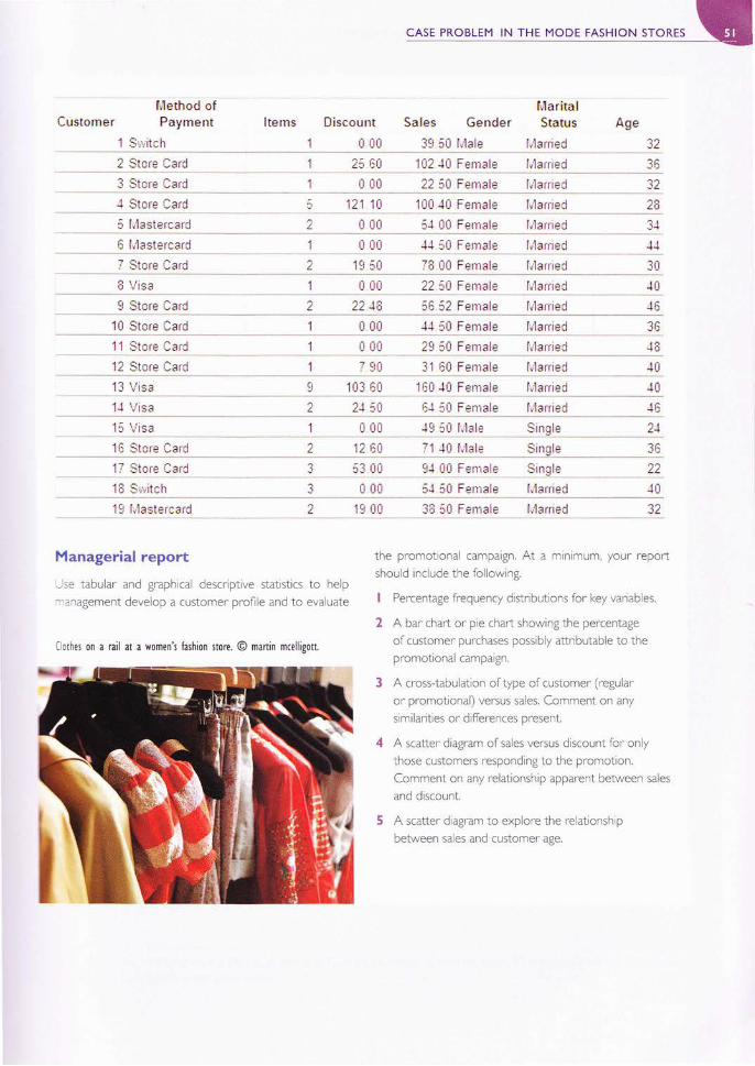
CASE PROBLEM IN THE MODE FASHION STORES

Customer Items Discount

r 9!0

1 __ q!05 .lal]O

_ 2 _ rloti

1 - Ú{0

2 19 50

Sales Gender

39 í! l-il!*102 ]Ü Fenrale

?2 5! Fqrlalg

!00 r! Flll.- - 51 0ü |-e11a]e

_ _ {J 5it fgyale7i] 0ű Ferriale

Ageaa,tz

.,u?a-tL-- - ""

--!r-- JJ

30

I _!!q ___2- , ??1F _

1 000

zz s0_19!1q!9

r!- i?-[-"-!,q1.

29 5Ü Feniale

31 !0 Fg-11ale

19! ]Ü |911ale6J itJ Fenrale

r!l i! lilrl.i1 JCt tJale

9J 00 Fsrriale

["1arrieC

-!,'!91igd:-""lJ 5Ü Fenrale Í'"1arriecl

_l!{cI Store Card

'lÜ Store Card -1 ll

1 Ü00

1 _ lgcl

_ I 1q!602 il50

_ 9002 12 Ett

: i3003 Ü00

l;larried

!:13t i*ll."larried

,- :1q;lÜ

+íJ

!l9!'{ J6

JL

,si1gl-e _

Single

SinEle

z4-;^-. .;:

]íá] 5Ú |9pa|e lJarried

2 19 0ir 30 50 Ferrrale l;l.criied

Managerial report

-se tabular and graphical descriptive statistics to help--anagement develop a customer prof le and to evaluate

I othes on a rail at a women\ íashion store. @ manin mcelligott.

the promotonal campagn. At a m n mum, your repoft

shou d include the íollowing'

l Percentage írequency distributions íor l<ey varrab|es'

2 A bar chart or p e chart showing the percentage

oí customer purchases possibly attributable to thepromotional campaign,

3 A cross-tabu|ation oítype of customer (regu|ar

or promotional) versus sales. Comment on any

similaritres or differences present,

4 A scatter diagram oí sa es versus d scount íor on y

those customers responding to the promotion.

Comment on any relationship apparent between sales

and d scount.

5 A scatter diagram to explore the relationship

between sales and custon'rer age,

Software Sectionfor Chapter 7

MINITAB offers extensive capabilities for constructing tabular and graphical summariesof data. In this section we show how MINITAB can be used to constn.rct several graphicalsummaries and a cross-tabulation. The graphical methods presented are the dot plot, thehistogram and the scatter diagram.

Dot plotAssume the audit times data of Table 2.4 are inThe following steps will generate a dot plot.

SteplGraph>Dotplot

Step 2 Select One Y, SimpleClick OK

Step 3 Enter C I in the Graph Variables boxClick OK

HistogramAgain, assume the audit times data are in column Clfollowing steps will generate a histogram.

SteplGraph>Histogram

Step 2 Select SimpleClicl< OK

Step 3 Enter Cl ln the Graph Variables boxClick OK

column C1 of a MINITAB worksheet

!"1ain menu bar]

fDotplots panel]

fDotplot - One Y, Simple panel]

of a MINITAB worksheet. The

lYain menu bar]

IHistogram panel]

[Histogram - Simple panel]

52

TABULAR AND GRAPHICAL PRESENTATIONS USING MINITAB

When the Histogram appears:

Step 4 Position the mouse pointer over any one of the bars, and Double ClickSelect the Binning tab [Edit Bars panel]Select Midpoint for lnterval TypeSelect Midpoint/Cutpoint positions for lnterval DefinitionEnter l2z32l5 in the Midpoint/Cutpoint positions boxxClicl< OK

Scatter diagramWe use the hi-fi equipment store data in Table 2.12 to demonstrate the construction of ascatter diagram. The weeks are numbered from I to 10 in column C1, the data for numberof commercials are in column C2. and the data for sales are in column C3 of a MINITABworksheet. The following steps will generate the scatter diagram shown inFigure 2.7.

Step I Graph > Scatterplot

Step 2 Select SimpleClick OK

Step 3 Enter C3 under Y VariablesEnter C2 under X VariablesClick OK

lYain menu barl

[Scatterplot panel]

[Scatterplot - Simple panel]

Cross-tabulationWe use the data from the restaurant review of section 2.4,part of which is shown in Table2.9, to demonstrate. The restaurants are numbered from 1 to 300 in column Cl of theMINITAB worksheet. The quality ratings are in column C2, and the meal prices are incolumn C3. MINITAB can create a cross-tabulation only for qualitative variables, so weneed to first code the meal price data by specifying a category (class) to which each mealprice belongs. The following steps will code the meal price data to create four categoriesof meal price in column C4: €I0-l9, €20-29' €30-39 and €4019.

Step I Data > Code > Numeric to Text fYain menu bar]

Step 2 Enter C3 in the Code data from columns box [Code - Numeric to Textpanell

Enter C4 in the Store coded data in columns boxEnter I0: I9 in the flrst Original values boxEnter € l0-l9 in the first New box

Repeat the last two operations using )0:29,30:39 and 4a:49 in the second, thirdand fourth original values boxes, and using €20 29' €30-39 and €40 49 in

the second, third and fourth New boxes,Click OK

*The entry 1.2:3515 indicates that 12 is the midpoint of the first class, 32 is the midpoint of the last class,and 5 is the class width.


For each meal price in column C3 the associated meal price category will now appearin column C4. We can now construct a cross-tabulation for quality rating and the mealprice categories by using the data in columns C2 and C4. The following steps will createa cross-tabulation containing the same information as shown in Table 2. 10.

Step 3 Stat > Tables > Cross Tabulation and Chi-Square lMain menu bar]

Step 4 Enter C2 in the For rows box [Cross Tabulation and Chi-Square panel]Enter C4 in the For columns boxSelect Counts under DisplayClick OK

EXCEL offers extensive capabilities for constructing tabular and graphical summariesof data. In this appendix, we show how EXCEL can be used to construct a frequencydistribution, bar chart, pie chafi, histogram, scatter diagram and cross-tabulation. We willdemonstrate two of EXCEL's most powerful tools for data analysis: creating charts andcreating PivotTable Reports.

Frequency distribution and bar chartfor qualitative dataIn this section we show how EXCEL can be used to construct a frequency distributionand a bar chart for qualitative data. We illustrate each using the data on soft drink pur-chases in Table 2.1.

F requ ency distribution

We begin by showing how the COUNTIF function can be used to construct a frequencydistribution. Refer to Figure 2.10 as we describe the steps involved. The formula work-sheet (showing the functions and formulae used) is set in the background, and the valueworksheet (showing the results obtained using the functions and formulae) appears inthe foreground.

The label 'Brand Purchased' and the data for the 50 soft drink purchases are in cells.A1:451. We also entered the labels'Soft Drink'and'Frequency'in cells C1:D1. Thefive soft drink names are entered into cells C2:C6. EXCEL's COUNTIF function cannow be used to count the number of times each soft drink appears in cells A2:A51. Thefollowing steps are used.

Step I Select cell D2

Step 2 Enter :COUNTIF($A$2:$A$5 I,C2)

Step 3 Copy cell D2 to cells D3:D6

The formula worksheet in Figure 2.10 shows the cell formulae inserted by applying thesesteps. The value worksheet shows the values computed by the cell formulae. This work-sheet shows the same frequency distribution that we constructed inTable 2.2.

TABULAR AND GRAPHICAL PRESENTATIONS USING EXCEL

Figure 2.10 Frequency distribution for soft drink purchases constructed using EXCEL'sCountif funCion

ABrand PurchasedCoke Classic

Diet Coke

Pepsi-Cola

Diet Coke

Coke Classic

Ccke ClassicDr Pepper

Diet Coke

Pepsi-Cola

Pepsi-Cola

Pepsi-Cola

Pepsi-Cola

Coke ClassicDr Pepper

Pepsi-Cola

Sprite

BCSoft Drink

Coke ClassicDiet Coke

Dr Pepper

Pepsi-Cola

Sprite

1

:rt

1-lA

:sIi0.'-+f{6{:'

+ü

+9

5Ü

51

DFrequency

=COUI'IT|F{SAS2 SASS 1 C2?

=COUI jT|F(SAS2.SAS5 1 C3i

=COUÍ,jTIFiSAS2 5A'55 1 c"l;

=COUIJT|Fi$AS2 SAS51 C5:

=COUI'ITIF{SA.S2 SA55 1 CSi

ABrand Purchased

Coke Classic

Diet Ccke

Pepsi-Cola

Diet Coke

Coke Classic

Coke Classic

Dr Pepper

Diet Ccke

Pepsi-Cola

Pepsi-Ccla

Pepsi-Cala

Pepsi-Cola

Coke Classic

Dr Pepper

Pepsi-Cola

Sprite

BCSoft Drink

Coke Classic

Diet Coke

Dr Pepper

Pepsi-Cola

Sprite

Í\lJ

Frequency19

o

5

13

U

Bor chort

Here we show how EXCEL's chart tools can be used to construct a bar chart for thesoft drink data. Refer to the frequency distribution shown in the value worksheet ofFigure 2.10. The bar chart that we are going to develop is an extension of this worksheet.The worksheet and the bar chart developed are shown in Figure 2.1I. The steps are asfollows:

Step ! Select celis C2.D6

Step 2 Click the lnsert tab on the Ribbon

Step 3 ln the Charts group, click Column


Step 3 ln the Charts group, clicl< Scatter

Step 4 When the list oí scatter diagram subtypes aPpears:Click Scatter with only Markers (the chart ln the upper-left corner)

Step 5 ln the Chart Layouts group, clicl< Layout I

Step ó Select the Chart Title and rep|ace it with Scatter Diagram for the H-FiEquipment Store

Step 7 Select the Horizontal (Value) Axis Title and replace it with Number ofCommercials

Step I Select the Vertical (Value) Axis Title and replace it with Sales Volume

Step 9 Right-click the Series I Legend EntryClick Delete

Step l0 Right click the vertical axisClick Format Axis

Step I I When the Format Axis panel appears:Go to the Axis Options sectionSelect Fixed for Minimum and enter 35 in the corresponding boxSe ect Fixed for Maximum and enter ó5 n the corresponding boxSelect Fixed for Major Unit and enter 5 in the corresponding boxCl cl< Close

A trendline can be added to the scatter diagram as follows.

Step l2 Posit on the mouse pointer over any data point in the scatter diagram and right-click to display a list of options

Step l3 Choose Add Trendline

Step I4 When the Add Format Trendline dialog box appears:Go to the Trendline Options sectronChoose Linear in the Trend/Regression Type sectionC lck Close

The worksheet in Figure 2.13 shows the scatter diagram with the trendline added.

PivotTable reportEXCEL's PivotTable Report provides a valuable tool for managing data sets involvingmore than one variable. We will illustrate its use by showing how to develop a cross-tabulation using the restaurant data in Figure 2.14. Labels are entered in row l, and thedata for each of the 300 restaurants are entered into cells A2:C301.

Creoting the initial worksheet

The following steps are needed to create aReport and PivotTable Field List.

worksheet containing the initial PivotTable


Figure 2.14 EXCEL wor*sheet containing restaurant data

''....--:-..."": A i B : CRestaurant Quality Rating Meal Price {€}

1j,-''*'"."..*''.i

"rlJ:

{.]:

É-.1lt:

"' -...-.-.- .;

8_l

9l-*- .'*-'l

t0 I

lt i

)o)^-"*-----'i

?o?--'*--"j

294;-*-*-**i

2esi,,.*-_)

?9ő]

t91l298i""."^*{?oo;**-*-i

19_qj

301 i

3q3j

1 Good

2 Very Good

3 Good

4 Excellent

5 Very Good

6 Good

7 Very Good

I Very Good

9 Very Good

10 Good

291 Very Gocd

292 Very Good

293 Excellent

294 Good

295 Good

296 Good

297 Good

298 Good

299 Very Good

300 Very Good

18

22

28

38

33

28

19

11

23

13

23

24

45

14

18

17

16

15

38

31

Step l Click the lnseÉ tab on the Ribbon

Step 2 ln the Tables group, click the icon above PivotTable

Step 3 When the Create PivotTable panel appears:Choose Select a table or rangeEnter Al:C30 ! in the Table/Range boxSelect New WorksheetClick OK

The resulting PivotTable Field List is shown in Figure 2.15.


Figure 2.l5 PivotTable Íleld list

PivotTabl* field LtÉt

Choose fields to add to report:

vxl:nH-l;ry t:

IRestaurantDQuality Reurrg

f]I'lealPrice {á

Drag fields betireen areas belor'.':

\í Repori Filter t't Cciumn tabels

:ia:i!iJ,t

a!a:!,:iii:_---,-- _.--,_-,.-_ -. -,-*. - -._,!

1r.J Rovr Labelst*-*-*--***--.*'- *-"*l:i

E Values

, Oeftr Layout Update

Using the PivotToble Fie/d List

Each column in Figure 2.14 (Restaurant, Quality Rating, and Meal Price) is considered afield by EXCEL. The following steps show how to use EXCEL's PivotTable Field Listto move the Quality Rating field to the row section, the Meal Price (€) Íield to the columnsection, and the Restaurant field to the values section of the PivotTable report.

Step I ln the PivotTable Field List, go to Choose Fields to add to report:Drag the Quality Rating Íle|d to the Row Labels area

Drag the Meal Price (€) ae d to the Column Labels area

Drag the Restaurant field to the Values area


Figure 2.l ó Completed PivotTable Í]eld list and a portion of PivotTable Repor1

D iATFivotTablé FieE Ligt

Choose fiekis to add to Íeport: t:lCormt of Restaurant \,Ieal Price (€) i'10 11 12 -+l It 3rand Total

LrcellentGood\.err Good

f

6

il1

J

_t 1

66

EIi50

Grarrd Totá I 6 1 J 30c

lB Restaumntllfl oualitv Raunoi--]M tteal Price (€)!

I

l

--*lDrag frelds bet'neen areas belo*:

Y neportriler ffi colr.mnt-áels

- il*J;*(e-;-lr,l :iri---i i-----,-,*á Rc'* Labels

' vclues

[] DeíErlayoutupdate

Step 2 Click Sum of Restaurant in the Values area

Click Yalue Field Settings

Step 3 When the Value Field Settings panel appears:

Under Summarize value field by, choose CountClick OK

Figure 2.16 shows the completed PivotTable Field List and a portion of the PivotTableReport.

Finalizing the PivotTable Report

To complete the PivotTable Report, the following steps are used to group the columnsrepresenting meal prices and place the row labels for quality rating in the proper order.

Step I Right-click in cell 84 or in any other cell containing meal pricesSelect Group

Step 2 When the Grouping panel appears:Enter l0 in the StaÉing at boxEnter 49 in the Ending at boxEnter I0 in the By boxClick OK


Figure 2,I 7 Final PivotTable Report

&

Step 3 Right-click on Excellent in ce I 45Choose MoveSelect Move "Excellent" to END

Step 4 Close the PlvotTable Fleld Llst dialog box

The final PivotTable Report is shown in Figure 2.17. Note that it provides the sameinformation as the cross-tabulation shown in Table 2. 10.

L)

1

;-1

I

:$:*

*

1r:

Ü*unt pí Restauranl í''i*a] Price Él **uaiit 'r Ratina 1Ü-1s 2Ü'29 3Ü_3s -í0-1! Grand Total

Gnod

Ysry' ücod

Exrelleni

414Ü234 E-1 .1i5 F,

l1J2E?2

Ü+

15Ü

6É

Grand Total iD ttn 76 3Ü |:

PASW offers extensive capabilities for constructing tabular and graphical summaries ofdata. In this section we show how PASW can be used to construct a histogram, a scatterdiagram, and a cross-tabulation.

HistogramAssume the audit times data of Table 2.4 are in the first column of the PASW DataEditor. The following steps will generate a histogram.

Step I Graph > Chart Builder |Yain menu bar]

Step 2 Under Gallery, choose Histogram fChart Builder panel]Drag and drop the Simple Histogram icon into the Chart Preview areaDrag and drop the audit t mes variable to the X-axis area in Chart PreviewC lcl< OK

Scatter diagramWe use the hi-fi equipment store data in Table 2.I2 to demonstrate the construction ofa scatter diagram. The weeks are numbered from 1 to 10 in the first column of the DataEditor, the data for number of commercials are in column 2 and the data for sales are incolumn 3. The following steps will generate the scatter diagram shown in Figure 2.7.

l

IABU!4! 4Nq GR4PHICAL pRESENrAloNs ustNG ar,a !

Drag and drop the Simple Scatter icon into the Chart Preview areaDrag and drop the sales volume varjable to the Y-axis area in Chart PreviewDrag and drop the number of commercials variable to the X-axis area in ChartPreviewCllcl< OK

Cross-tabulationWe use the data from the restaurant review of section 2.4, part of which is shown in Table2.9, to demonstrate. The restaurants are numbered from i to 300 in the first column ofthe PASW Data Editor. The quality ratings are in column 2 and the meal prices are incolumn 3. PASW can create a cross-tabulation only for categorized variables, so we needto Írrst code the meal price data by speciÍying a category (class) to which each meal pricebelongs. The following steps will code the meal price data to create four categories ofmeal price in column 4: €l0-19, €20-29, €30-39 and€4049.

Step I Transform > Recode lnto Different variables fMain menu bar]

Step 2 Transferthe meal price vadable to the lnput Variable->Output Variable box

fRecode !nto Different variables panel]Under Output Variable, give the new variable a name and labelClick ChangeClicl< OId and New Values

Step 3 Under Old Values, check Range, and enter l0 and l9 in the two boxes

fRecode lnto Different variables: Old and New Values panel]Under New Value, check Value and enter I in the boxClick Add

Step 3 aIlocates code l to the € l 0- l 9 meal price range' Repeat this step for the)0 29,30-39 and 40-49 ranges, allocatingthem codes 2,3 and 4 respectively,

Clicl< Continue

Step 4 Click OK [Recode lnto Different variables panel]

The new categorized variable will be added to the Data Editor, in column 4.Appropriate labels can be defined for the codes of this new variable in the Variablesview of the Data Editor.

We can now construct a cross-tabulation for quality rating and the meal price catego-ries by using the data in columns 2 and 4 of the Data Editor. The following steps willcreate a cross-tabulation containing the same information as shown in Table 2.10.

Step I Graph > Chart Builder

Step 2 Under Gallery, choose Scatter/Dot

Step 5 Analyze > Descriptive Statistics > Crosstabs

Step ó Transíer the qua|ity ratrng varabJe to the Rows boxTransfer the new meal price variable to the Columns boxClick OK

[Main menu bar-

[Chart Builder panel]

[Main menu bar]

[Crosstabs pane ]

cHAPTER 3 DESCRIPTIVE STATISTICS: NUMERICAL MEASURES

In (3.1), the numerator is the sum of the values of the n observations. That is,

2x.: xrl x, l "'l r,

The Greek letter I is the summation sign.To illustrate the computation of a sample mean, consider the following class size data

for a sample of five university classes.

46 54 42 46 32

Weusethenotation xr,x2,x3,x4,x5to representthenumberof studentsineachof thefive classes.

x, : 46 xr: 54 x, : 42 x.: 46 xr: 32

To compute the sample mean, we can write

x,*xr*x.*x^lx, 46+54+42+46+32 :44

The sample mean class size is 44 students.Here is a second illustration. Suppose a university careers office has sent a question-

naire to a sample of business school graduates requesting information on monthly start-ing salaries. Table 3.1 shows the data collected. The mean monthly starting salary for thesample of 12 business school graduates is computed as

x, I xr* "' I xr, _ 2O2O + ZO?s + ... + ZO4O

Equation (3.1) shows how the mean is computed for a sample with n observa-tions. The formula for computing the mean of a population remains the same, butwe use different notation to indicate that we are working with the entire population.We denote the number of observations in a population by N, and the population meanas p.

>Á._lx:-:n

12I2

>,x._lx:

-:n24 840 : 20.70

I2

GraduateMonthly starting salary

(€) GraduateMonthly starting salary

(€)

I

z3

4

5

6

7070

74757125

7040r 980

I 955

7

I9

t0lttz

2050)t 65

2074))602460)a4a

MEASURES OF LOCATION

Again, because I is an integer, step 3(b) indicates that the third quartile, or 75th percen-tile, is the average of the ninth and tenth data values; hence,

Q.: (2'075 + 2rZ5)12:2100.

The quartiles divide the starting salary data into four parts, with each part containing25 per cent of the observations.

lgss 1980 2O2O|2O4O 2O4O

Q,:20302050 | 2060 2070 2O75|2Í25 2165 2260

Qr:2055 Q.:2100(Median)

We defined the quartiles as the 25th, 50th and 75th percentiles. Hence, we computedthe quartiles in the same way as percentiles. However, other conventions are sometimesused to compute quartiles and the actual values reported for quartiles may vary slightlydepending on the convention used (see the Software Section at the end of the chapter).Nevertheless, the objective of all procedures for computing quartiles is to divide the datainto four equal parts.

MethodsI Considerasamplewithdatavaluesof 10,20, 12, lTand l6.Computethemeanandmedian.

2 Consider a sample wrth data values oí | O, 20' zl ' 17, 16 and l 2. Compr_r|e the mean and median.

3 Consider a sample with data values oí 27, 25' 20' l 5' 30' 34' 28 and 25. Compute the 2oth,

25th, 65th and 75th percentiles,

4 Consider a sample with data values of 53, 55, 70, 58, 64, 57, 53, 69, 51, 68 and 53. Compute

the mean, median and mode,

Applications5 A sample of 30 lrish engineering graduates had the following starling salaries, Data are in

thousands of euros.

36.8 34,9 35.2 37.2 36.2 35 I 36 8 36. | 36.7 36.6

31.3 38.2 36.3 36.4 39.0 38.3 36.0 35.0 36.7 31.9

38.3 36,4 36 5 38.4 39.4 38.8 35.4 36.4 37 .0 36.4

a. What is the mean starting salary?

b. What is the median starting salary?

c, What is the mode?

d. What is the Ílrst quarti|e?

e. What is the third quartile?

ó The íollowing data were obtained for the number of minutes spent listening to recorded

musrc for a sample of 30 individuals on one particular day.

88.3 4,3 4.6 7 .0 9.2 0 0 99.7 34.9 8l .1

85.4 0.0 t7 .5 45.0 53.3 Z9.1 28.8 0.0 98.9

4.4 67.9 942 L6 56.6 52..9 145.6 70.4 65. I

0.0

64.5

63.6

CHAPTER 3 DESCRIPTIVE STATISTICS: NUMERICAL MEASURES

a. Compute the mean.

b. Compute the median,

c, Compute the Ílrst and thlrd quaft les.

d. Compute and interpret the 4fth percenti e.

minlRank (w.ww.minrrank.com) rates the populartty of websttes tn most countries of the

word, using a points system. The 25 most popular sites in Cyprus as listed rn November

2O0B were as follows (the po nts scores have been rounded to one decimal place):

Website Points Website Points

www.dad.com,cywr,vw.dvds.com,cy

wlvw.íitness'com 'cy

w ww,ai rl inetrckets.com.cy

w ww.weightloss.com.cy

www,cyprus.gov.cy

www.netcars,com,cy

wtr,w,vis itcypru s. org. cy

w^ww'í|owershop'com'Cy

wvrw'netinío'com 'cyw wvr,interprom.cy

www.c)ta.com.cy

www.drivenet,com,cy

www,ch ris-mr chael.com.cy

w ww.music.net.cy

drivenet.com.cy

www.prismastore.com.cy

w^vtw'íorce'com.cy

www.prisma.com.cy

www.prismanet,cy

wr.lvr,ebos.com.cy

w ww.cytanet.com.cy

www,hrdauth,org.cy

wvvw.ucy.ac.cy

w ww,eplaza.com,cy

59.)21020.s

200t9.B

t].314.3

t4.3

t3lt).5

959.4

9.1

BB8.7

868,6

B5B58.5

736.1

6.7

\R57

a, Compute the mean and median,

b. Do you think it would be betterto use the mean orthe median as the measure oícentral location for these data? Explain.

c. Compute the lrst and third quar1l es,

d. Compute and interpret the 85th percentile.

Fol owing is a sample oí age data íor indlv dua|s working írom home by 'telecommuting''

rB 5'1 2a 46 25 48 53 )7 )6 37

40 36 42 25 )7 33 28 4a 45 75

a. Compute the mean and the mode,

b. Suppose the median age oíthe population oíalI adu|ts is 35.5 years' Use the median age

of the preced ng data to comment on whether the at-home workers tend to be younger

or older than the population oí all adults.

c. Compute the flrst and third quaftiles,

d. Compute and interpret the 32nd percent le.

In addition to measures of location, it is often desirable to consider measures ofvariability, or dispersion. For example, suppose you are a purchasing agent for a largemanufacturing firm and that you regularly place orders with two different suppliers.After several months of operation, you find that the mean number of days required tofiIl orders is ten days for both of the suppliers. The histograms summarizing the numberof working days required to fill orders from the suppliers are shown in Figure 3.2.Although the mean number of days is ten for both suppliers, do the two suppliersdemonstrate the same degree of reliability in terms of making deliveries on schedule?

MEASURES OF VARIABILITY

Coefficient of variation

(Standard deviation

Meanx roo)% (3.8)

For the class size data, we found a sample mean of 44 and a sample standard deviationof 8. The coefficient of variation is [(8/aa) x 100]Vo : 18.27o. The coefficient of varia-tion tells us that the sample standard deviation is 18.2 per cent of the value of the samplemean. For the starting salary data with a sample mean of 2010 and a sample standarddeviation of 82.2, the coefficient of variation,IG2.2/2010) X 10017o : 4.0Vo, tells usthe sample standard deviation is only 4.0 per cent of the value of the sample mean. Ingeneral, the coefficient of variation is a useful statistic for comparing the variability ofvariables that have different standard deviations and different means.

Methods9 Conslderasamp|ewithdatava|uesoíl0'20 |), lf and l6.Calcu|atetherangeand

interquarlile range.

l0 Considerasamplewithdatavaluesof 10,20 l2, 17and l6.Calcuiatethevarianceandstandard deviation.

ll Considerasamp|ewithdatavaluesoí27,25,20, l5 30 34,28and25.Ca|cu|atetherange,interquart le range, variance and standard deviation.

Applicationsl2 Abatsman'scricketscoresforsixrnnrngswere4l,34,42,45,35and3T.Usingthesedataas

a sample, compute the íol1owlng descriptive statistics.

a. Range.

b. Vanance.

c. Stancard devialon.d' CoefÍlc ent oí var]ation.

l3 Dinner bi|| amounts íor set menus at a Dubal restaurant, A| Khayam, show the fo||owing

lrequency distnbution. The amounts are ln AED (Emirati dirham). Compute the mean,

variance and standard deviatron,

Dinner bill (AED) Frequency

30

4050

60

7A

80

Total

2

6

4

4

7

7

20


! 4 The following data were USed to construct the h istograms oí the num ber of days req u ired toílll orders íor Dawson Supply and íor-J.C. Clark Distributors (see Figure 3.2).

Dowson Supply doys for delivery:

Aak Distributors days for delivery:

l t0 9 l0 l ! t0 | t0 t0

8t0t37t0lt07t512Use the range and standard deviation to suppoft the previous observation that DawsonSupply provides the more consistent and reliable delivery times.

l5 Po|ice records show the íol|owing numbers oí daily crime reports íor a sample oí days dudng

the winter months and a sample of days during the summer months,

Winter:

Summer:

18 20 15 t6 7t

78 18 74 32 18

z0 12 ló 19 z029 23 38 2B t8

a. Compute the range and interquartile range íor each period.

b. Compute the variance and standard deviation for each period.

c. Compute the coeÍÍlclent oívadatlon íor each penod.

d, Compare the variability of the two periods.

l ó A production department uses a sampling procedure to test the quality of newly produceditems, The department employs the following decision rule at an inspection station: ií asampe oí l4 tems has a variance oímore than 0.005' the production ine must be shutdown íor repairs. Suppose the íollowing data have just been co|lected:

3.43 3.45

3 48 3.41

Should the production line be shut down? Why or why not?

We described several measures of location and variability for data distributions. It is alsooften important to have a measure of the shape of a distribution. In Chapter 2 we notedthat a histogram offers an excellent graphical display showing the shape of a distribution.An important numerical measure of the shape of a distribution is skewness.

Distributional shapeFour histograms constructed from relative frequency distributions are shown inFigure 3.3. The histograms in Panels A and B are moderately skewed. The one inPanel A is skewed to the left: its skewness is -0.85 (negative skewness). The histo-gram in Panel B is skewed to the right: its skewness is +0.85 (positive skewness).The histogram in Panel C is symmetrical: its skewness is zero. The histogram in PanelD is highly skewed to the right: its skewness is 1.62. The formula used to compureskewness is somewhat complex.x However, the skewness can be easily computedusing statistical software (see Software Section at rhe end of this chapter).

*The formula for the skewness of sample data:

Skewness - r-;,r -rt(=)

3.43 3 48 3.52 3.s0 3.39

3.38 3.49 3 45 3.5 | 3.s0


Detecting outliersSometimes a data set will have one or more observations with unusually large or unusu-ally small values. These extreme values are called outlÍers. Experienced statisticians takesteps to identify outliers and then review each one carefully. An outlier may be a datavalue that has been incorrectly recorded. If so, it can be corected before further analysis.An outlier may also be from an observation that was incorrectly included in the data set.If so, it can be removed. Finally, an outlier may be an unusual data value that has beenrecorded correctly and belongs in the data set. In such cases it should remain.

Standardized values (z-scores) can be used to identify outliers. The empirical ruleallows us to conclude that for data with a bell-shaped distribution, almost all the datavalues will be within three standard deviations of the mean. Hence, we recommend treat-ing any data value with a z-score less than -3 or greater than f3 as an outlier, if thesample is small or moderately sized. Such data values can then be reviewed for accuracland to determine whether they belong in the data set.

Refer to the z-scores for the class size data in Table 3.4. The z-score of - 1.50 showsthe fifth class size is furthest from the mean. However, this standardized value is wellwithin the -3 to *3 guideline for outliers. Hence, the z-scores do not indicate thatoutliers are present in the class size data.

Methods17 Consider a sample with data values oí l0, 20, |2, 17 and | 6. Calculate the z-score íor each

oíthe five observations.

l8 Consider a sample with a mean of 500 and a standard devlation oí |00' What are theZ-scores íor the íol]owing data values: 520, 650 500 450 and 2BO?

l9 Consider a sample with a mean of 30 and a standard deviation of 5. Use Chebyshev'stheorem to determine the percentage of the data within each of the following ranges.

a. 20 to 40 b. l5 to 45 c. zZto 38 d. l8to42 e. l2to48

MEASURES OF DISTRIBUTIONAL SHAPE, RELATIVE LOCATION AND DETECTING OUTLIERS

20 Suppose the data have a bell-shaped diírjbution with a mean oí 30 and a standard deviation of 5'

Use the empirica| rule to determlne the percentage oí data within each of the ío|lowing rarrges'

a, 20to40 b. 5to45 c, 25to35

Applications2l Theresutsoíasurveyof l54adultsshowedthatonaverage'adu]tsseep6'9hoursperday

during the working week. Suppose that the standard deviation is 1.2 hours,

a, Use Chebyshevs theorem to calculate the percentage of individuals who sleep between4.5 and 9.3 hours per day,

b' Use Chebyshev's theorem to calcu ate the percentage oí individuals who sJeep between3.9 and 9.9 hours per day,

c, Assumethatthenumberofhoursofsleepfollowsabell-shapeddistribution,Usetheemprdcal rule to calculate the percentage of ind v duals who s eep between 4.5 and

9.3 hours per day. How does this result compare to the value that you obtained using

Chebyshev's theorem in part (a)?

22 Suppose that lQ scores have a be _shaped distr]but]on with a mean oí 0O and a standard

deviation of 15.

a. Whatpercentage oípeop|e have an |Q score between 85 and ll5?b, What percentage of people have an lQ score between 70 and 130?

c. What percentage oí people have an |Q score oí more than l30?

d, A person with an lQ score greater than 145 is considered a genius. Does the empidcalrule supporl thls statement? Explain,

23 Suppose the average hourly labour cost for car servrcing in lohannesburg s ZAR(South Aírican rand) 75.00, and the standard deviation is ZAR 20.00.

a. What is the z-score íor a car serv ce wtth an hour|y ]abour cost oí ZAR 5ó 00?

b. What is the z-score íor a car serv ce with an hour|y ]abour cost oí ZAR l 53'00?

c. lnterpret the z-scores in parts (a) and (b). Comment on whether either should be

considered an outlier,

24 Consumer Reylew poícs revlews and ratings of a varlety oí produccs on the ntemet' The ío |owing

is a sample of 20 speakersystems and their ratings, on a sca|e oí | to 5, with 5 being best.

a. Compute the mean and the median,

b. Compute the f rst and thlrd quart les,

c. Compute the standard deviation.

d, The skewness of this data is 1.67. Comment on the shape of the distribution,

e, What are the z-scores associated with Allison One and Omni Audio?í Do the data contain any outliers? ExpLain'

Speaker Rating Speaker Rating

InÍinity Kappa 6' I

Allison OneCambridge Ensemble ll

Dynaudio Contour 1.3

Hsu tuch. HRSWI2VLegacy Audio Focus2ó Mission 73liPSB 4OOi

Snell Acoustics D lVThiel CS 1.5

ACI Sapphire lll

Bose 50 I SeriesDCM KX.2I2Eosone RSFl000

loseph Audio RMTsiYlarlin Logan AeriusOmni Audio SA l2 3

PolkAudo RTl2SunÍlre True SubwooíerYamaha N5-A636

4.004.t)_

3824004.564374.33

4.504.644.)O

4.677.t44.094.17

4884.76).374,504.t72.17

EXPLORATORY DATA ANALYSIS

In Figure 3.5 we included lines showing the location of the upper and lower limits.These lines were drawn to show how the limits are computed and where they are locatedfor the salary data. Although the limits are always computed, generally they are notdrawn on the bÓx plots. Figure 3.6 shows the usual appearance of a box plot for the sal-ary data. Box plots provide another way to identify outliers. But they do not necessarilyidentify the same values as those with a z-score less than -3 or greater than +3. Either,or both, procedures may be used.

Methods25 Consider a sample with data values of 27, 25, 20, I 5, 30, 34, 28 and 25. Provide the five-

number summary íor the data,

ző Construct a box plot for the data in Exercise 25'

27 Prepare the five-number summary and the box plot for the following data: 5,

t2, 16, tO,6.

t8, t0,8,

28 A data set has a Íirst quartile of 42 and a third quartile of 50. Compute the lower and

upper limits íorthe corresponding box plot' Should a oata Value oí65 be consideredan outlied

UpperLimit

I

I

I

flOR)J

1800 1900 2000 2100 2200 2300


Applications29 Annua| sales, in mi||ions oídollars' íor 2l pharmaceutical companies follow

8408 t374 tB72 8879 7459 I t4t 3 60814 r 38 6457 | 850 28 I B I 356 I 0498 747840t9 434t 139 7t)1 3653 5794 8305

a. Provrde a Ílve-number summary'

b' Compute the lower and upper limits (íorthe box plot).

c. Do the data contain any outliers?

d. Johnson & Johnson's sales are the largest on the list at $ l4 I 38 milllon, Suppose a

data entry error (a transposition) had been made and the sales had been entered as

$4 l l38 million' Wouldthe method oídetecling outliers in part (c) identifythis prob|em

and allow for correction ofthe data entry error?

d. Construct a box plot,

A goal of management is to help their company eam as much as possible relative to thecapital invested' One measure oísuccess is return on equity _ the ratlo oí net income toíockholders' equity. Retum on equity percentages are shown here íor 25 companres'

9.0 t9.6 7).9 41.6 t t.4 15.8 57.7 t7.3 tZ.3 5. t

17.3 3t.t 9.6 8.6 lt.z t2.8 17.?, t45 9.2 16.6

5.0 30.3 t4.7 192 6.2

a' Provide a Ílve-number summary.

b. Compute the |ower and upper lim ts (íor the box p|ot)'

c. Do the data contain any outliers? How would this iníormation be helpíu| to a Í'inancial ana|yst?

d. Construcl a box plot.

In 2008, stock markets around the wodd lost vaiue. The website wvr'w.owneverystock,com

|isted the fo||owing percentage íal|s in stock market indices between the star1 oíthe year and

the beginning oí October.

Country % Fall Country % Fall

30

3t

New ZealandCanada

Switzerland

MexicoAustralia

KoreaUnited Kingdom

Spain

Malaysia

ArgentinaFrance

lsrael

GermanyTaiwan

Brazil 39.59japan 39,88

Sweden 40.35Egypt 4l.57Singapore 4lr.60

Italy 42.88

Belgium 43.70lndia 44.16Hong Kong 44.52Netherlands 44.61

Norway 46.98

lndonesia 47.13Austria 50.06China. 6024

27.05

27,30

28.47

29.99

3 r.95

32.t832.37

32.69

3)..86

36.83

37.71

31.84

37.85

38.79

a. What are the mean and median percentage changes forthese countries?b. What are the Ílrst and third quartiles?

c. Do the data contain any outliers? Construct a box plot.

d. What percenti|e would you report íor Belgium?

MEASURES OF ASSOCIATION BETWEEN TWO VARIABLES

variable causes the other. For instance, we may find that a restaurant's quality rating andits typical meal price are positively correlated. However, increasing the meal price willnot cause quality to increase.

Methods32 Five observations taken for two variables follow.

;,á,3]J;]:a. Construct a scatter diagram with the x, values on the horizontal axis.

b. What'dOes the scatter diagram developed in part (a) indicate about the relationshipbetween the twÖ variables?

c. Compute and interpret the sample covariance.d. Compute and interpret the sample corre.lation coefflcient.

33 Five observations taken for two variab|es íollow,

x, 6 ll 15 21 27y,69617tz

a. Construct a scatter diagram for these data.

b. What does the scatter diagram indicate about a relationship between X and )?c. Compute and interpret the sample covariance.d. Compute and interpret the sample correlation coefilcient.

Apptications34 PCWotd provided perlormance scores and ratings for l5 notebook PG. The perlormance score

is a measure of how fast a PC can run a mix of common business applications as compared to

50

40

30

20

10


a baseline machine. For example, a PC wrth a performance score of 200 is twice as fast as the

baseline machine. A 1OO-point scale was used to provide an overall rating for each notebook

tested in the study, with higher scores indicating a better rating. The data are shown below.

Notebook Performance score Overall rating

AMS Tech Roadster l5CTA380Compaq Armada M700

Compaq Prosignia Notebook 150

Dell lnspiron 3700 C466GTDell lnspiron 7500 R500WDe|| Latitude Cpi A36óXTEnpower ENP-3 l3 Pro

Gateway Solo 9300LS

HP Pavillion Notebook PCIBM ThinkPad I Series 1480

Micro Express NP7400Micron TransPort NX Pll-400

NEC Versa SXSceptre Soundx 5200Sony VAIO PCG-F340

lt5t9t153

t94736r84

t842t6r85

r83

l89702t92t4tt87

67

]B79

80

84

76

7l9)83

7B

77

78

78

73

77

a' Construct a scatter diagram with períonnance score on the horrzonta| ax]s.

b. Is there any relationship between performance score and overall rating? Explain,

c. Compute and intepret the sample covariance,

d. Compute and interpret the sample correlation coelTlcient,

e. What does the sample correlation coeíÍlcient te|l you about the relationship between theperíormance score and the overall rating?

35 The Dow.Jones lndustrial Average (DJIA) and the Standard & Poors (S&P) 500 lndex

are both used as measures of overall movement in the US stock market. The DJIA is based

on the price movements oí30 large companies; the S&P 500 ls an index composed oí500stocks. Some say the S&P 500 is a better measure oí stock market per'formance because it

is broader based. The index levels of the DJIA and the S&P 500 for l0 weeks beginning with

I July 2008 are shown below (file 'DowS&POB' on the accompanying CD).

Date DJrA s&P

I July8 july

l5 July77)uly29 )uly5 Augustl2 Augustl9 August26 August

2 September

1t 387.26

r I 384.21

t0 962.54

r r 602.s0I I 397.56

t I 615.77

t I 642.47

r | 348.55

I I 4t2.87I I 5169)

t284.91

t273.70

tzt4.9tt277.00

1763.70

r284.88

r289.59

t266.69

127 t.51

t277.58

a.

b.

Compute the sample correlation coefflcient for these data.

Are they poorly correlated, or do they have a close association?


Audit time(days)

Classmidpoint (M,) Frequency ([)

Squared

deviation(M,- R)' ftM,- x7'

Deviation(M, - X)

l0-14t5-t920-241tr fo

30-34Total

124-7t] 8-)7)5377ZB,_ I 13

z0

Lf,(M, - i), stoSamplevariancet': n I

: 19:30

49

4

9

64

169

t963)_

45

t28

169

570

>fw,- r)'

Population mean for grouped data

, _2f, M,

tNPopulation variance for grouped data

ZfÍM, - lr),O7=

Methods3ó Consider the íollowing data and corresponding weights

x Weight

3262.0 3

)5 2

5.0 B

a. Compute the weighted mean,

b' Compute the sample mean oíthe íour data values without weighting' Note the difference

in the results provided by the two computations,

37 Consider the sample data in the following írequency distribution.

Class Midpoint Frequency

3-78-12

t3-t7t8-)7

4

7

9

5

(3. r 8)

(3. r e)N

5

t0

t5

z0

THE WEIGHTED MEAN AND WORKING WITH GROUPED DATA

a. Compute the sample mean.

b. Compute the sample vanance and sample standard deviation.

Applications38 Bloomberg Personal Finonce ()ulylAugust 200 I ) included the following companies in its

recommended investment portfolio. For a porLfolio value of €25 000, the recommendedeuro amounts allocated to each íock are shown.

Company Portfolio (€)Estimated Dividend

growth rate (%) yield (%)

CitigroupGeneral Electric

Kimberley-Clark

OraclePharmacia

SBC CommunicationsWoddCom

300055004700

3000300038002500

t5

t4

tz25

z0t235

t.zlt.4B

t.72

0.00

0.96

2.48

0.00

a. Using the portíolio euro amounts as the weights, what ls the weighted average estimated

growth rate forthe portfolio?

b. What is the weighted average dividend yield forthe portfolio?

39 A petro| station recorded the ío|lowing írequency distribution íorthe number of litres ofpetrol sold per car in a sample of 680 cars.

Petrol (litres) Frequency

r-t5I 6-303 t+546-606t-7576-90Total

74t92280t05

73

6

680

Compute the mean, variance and standard deviation íor these grouped data. líthe petrol

station expects to serye petrol to about I 20 cars on a given day, estimate the totalnumber of litres of petrol that will be sold.

For additional online summary questions and answers goto the companion website at www.cengage.co.uk/aswsbe2

oaaaaa aaaaaa aaaaaa...


Table 3.1 listed the starting salaries for 12 business school graduates. Panel A of Figure3.11 shows the descriptive statistics obtained by using MINITAB to summarize thescdata. Definitions of the headings in Panel A follow.

N number of data valuesN* number of missing data valuesMean meanSE Mean standard error of meanStDev standard deviation

Min minimum data value

Ql first quartileMedian median

Q3 third quartileMax maximum data value

The label SE Mean refers to the standard error of the mean,which is computed t';,

dividing the standard deviation by the square root of the number of data values. Thi.statistic is discussed in Chapter 7 when we introduce the topics of sampling and samplinsdistributions. Although the range, interquartile range, variance and coefficient of varia-tion do not appear on the MINITAB output, these values can be easily computed frorr-the results in Figure 3.11 as follows.

Range: Max-MinrQR:Q3-Q1

Variance : (StDev)'z

Coefficient of Variation : (StDev/Mean) X 100

Note that MINITAB's quartiles Q1 : 2025 and Q3 - 2112.5 are slightly differer.from the quartiles Q,: 2030 and Q.: 2100 computed in Section 3.1. The differen.conventionsx used to identify the quartiles explain this difference. The values providecby one convention may not be identical to the values by another convention, but the dif-ferences tend to be negligible so far as interpretation is concerned.

The statistics in Figure 3.ll are generated as follows. The starting salary data are ircolumn C2 of a MINITAB worksheet.

*With the n observations arranged in ascending order (smallest value to largest value), MINITAB use.the positions given by (n + l)l4 and 3(n + 1)l4tolocaÍe Q, and Q_,, respectively. When a position:,fractional, MINITAB interpolates between the two adjacent ordered data values to determine the cor-responding quartile.

t08

DESCRIPTIVE STATISTICS USING MINITAB

Step I Stat > Basic Statistics > Display Descriptive Statistics fMain menu bar]

Step 2 Enter C2 in the Variables boxClick OK

fDescriptive Statlstics panel]

Panel B of Figure 3.11 is a MINITAB box plot. The box drawn from the first to thirdquartiles contains the middle 50 per cent of the data. The line within the box locatesthe median. The asterisk indicates an outlier at 2260. The following steps generate thebox plot.

Step I Graph>Boxplot

Step 2 Select SimpleClick OK

Step 3 Enter C2 in the Graph variables boxClick OK

The skewness measure also does not appear as paÍt of MINITAB's standard descrip-tive statistics output. However, we can include it in the descriptive statistics display byfollowing these steps.

[Main menu bar]

[Boxplot panel]

[Boxplot - One Y, Simple panel]

Panel A

Descriptive statistics: starting salary (€}

'.rt=iebte }' 1'i* }{eaa 9E Mea:r Sg}ev !{ínintg *1 *edj.a*sEa:íieg sa].ary {€} L2 0 20?8.8 23.? ?2,2 ts55.ű 2825'0 205s.s

'r'ari-ab1e Q3 Y.axi&üÍeSta=ti'nq Salary {€} 2LL2.s 22ía.a

Panel B

Boxplot oÍ Starting Salary (€)

2200g,

h 21506ah

p zrooL(E

a zoso

2000

1 950


Step I Stat > Basic Statistics > Display Descriptive Statistics [Main menu b:-

IDescriptive Statistics par.

The skewness measure of 1.07 will then appear in your Session window.Figure 3.12 shows the covariance and correlation output that MINITAB provide:

for the hi-fi equipment store data in Table 3.5. In the covariance portion of the fig-ure, No. of Commercia denotes the number of weekend television commercials an;Sales Volume denotes the sales during the following week. The value in column No. c-

Commercia and row Sales Volume, 11.00, is the sample covariance as compute:in Section 3.5. The value in column No. of Commercia and row No. of Commerci;.2.22, is the sample variance for the number of commercials and the value in colurr,Sales Volume and row Sales Volume, 62.89, is the sample variance for sales. Th.sample correlation coefficient, 0.93, is shown in the correlation portion of the ou:-put. The interpretation and use of the p-value provided in the output are discussed i:Chapter 9.

To obtain the information in Figure 3.Í2, we entered the data for the number of corn-mercials into column C2 and the data for sales volume into column C3 of a MINITAEworksheet. The steps necessary to generate the covariance output are:

Step 2 Enter C2 in the Variables boxCl ck the Statistics button

Step 3 Check SkewnessCckOK

Step 4 Clck OK

[Descriptive Statistics par :

lDescriptive Statistics - Statistics par':

flYain menu b.'[Covariance pan:-

change is necessary tmenu (step 1), choos;

Step I Stat > Basic Statistics > CovarianceEnter C2 C3 in the Variables boxClick OK

To obtain the correlation output in Figure 3.12, only onethe steps for obtaining the covariance: on the Basic StatisticsCorrelation rather than Covariance.

'.'' . Covarianaéánd con elaiiáa, .oui6"6.fi_$.=iglNlTAB'íg=a.. -number:cÍ.c-o.mmercials

=:.. aÍ..ld sales€áta,

Covariances: No. of Commercials, Sales Volume

l'lo. ci Cc:rx,erciaH2 lé= 1r^lltYé

Correlations: No.

Eca*q^n n^-rsj ;r i ^n!-''.ia1ue = (t .8QÜ

tÍ^ ^-- ^^?féyF.i =

á a^^^^1. tazla11. !f,on(r

Q=ls= i.'^lrr+a

of Commercials, Sales Volume

ci I'l*. ci 3c:r:u,e:eia1s anC Sales r,;c!t:ne = 0.930

DESCRIPTIVE STATISTICS USING EXCEL

We show how EXCEL can be used to generate several measures of location andvariability for a single variable and to generate the covariance and correlation coefficientas measures of association between two variables.

Using EXCEL FunctionsEXCEL provides functions for computing the mean, median, mode, sample variance, andsample standard deviation. We illustrate the use of these EXCEL functions by computingthe mean, median, mode, sample variance and sample standard deviation for the startingsalary data in Table 3.1. Refer to Figure 3.13 as we describe the steps involved. The dataare entered in column B.

EXCEL's AVERAGE function can be used to compute the mean by entering thefollowing formula into cell E,1:

: AVERAGE(B2:B13)

Similarly, the formulae :MEDIAN(B2:B l3), :MODE(B2:B l3), :y4R(B2:B13), and:STDEV(B2:813) are entered into cells E2:85, respectively, to compute the median,mode, variance, and standard deviation. The worksheet in the foreground shows that thevalues computed using the EXCEL functions are the same as we computed earlier in thechapter.

= i--re 3.13 Using EXCELfunctions forcomputingthe mean, median, mode, variance and

standard deviation

.-- }J

;]':Uate Staning salary {€)

2020

- 2015

2ll1

- 20J0, 19S0_ l:3r- 2050

2Bt0

22e0

2060

: 20J0

v

iileaníiledianMode

VarianceStandard Deviation

AGraduate Starting

1

4I

3

+

5

6a

"o

I10

11

12

E

=AVERAGE(B2 B13i

=íJEDlAl'1iB2 B13;

=l'lODEi82 B13l

=VAR|82 B13l

=STDEV{B2 B13l

1

;_1

-l

á

ö

9

10

11

1l1_1

1{

1)!

Salary {€)

2020

2075

I ttJ20-r0

1 980

1 955

2050

I llJs

2070

ltbu2060

20J0

DEhlean

Ívledian

$,lode

VarianceStandard Deviation

2070

2055

20-r0

675.1 5

822


EXCEL also provides functions for computing the covariance and correlatio:-coefficient. You must be careful when using these functions because the covarianc;function treats the data as a population and the correlation function treats the data a.a sample. So the result obtained using EXCEL's covariance function must be adjustecto provide the sample covariance. We show here how these functions can be used r"

compute the sample covariance and the sample correlation coefficient for the stere-and sound equipment store data in Table 3.7. Refer to Figure 3.14 as we present th.steps involved.

EXCEL's covariance function, COVAR, can be used to compute the population cor-ariance by entering the following formula into cell Fl:

: COVAR(B 2:B r I,C2:CI I)

Similarly, the formula:CORREL(B2:B1I,C2:CI1) is entered into cell F2 to con-pute the sample correlation coefficient. The worksheet in the foreground shows tl:.values computed using the EXCEL functions. Note that the value of the sample co:-relation coefficient (0.93) is the same as computed using equation (3.12). Howere:the result provided by the EXCEL COVAR function, 9.9, was obtained by treating th:data as a population. We must adjust the EXCEL result of 9.9 to obtain the samp-:covariance. The adjustment is rather simple. First, note that the formula for the popul.-tion covariance, equation (3.11), requires dividing by the total number of observatior-.in the data set. But the formula for the sample covariance, equation (3.10), require.dividing by the total number of observations minus 1. So, to use the EXCEL result r r

9.9 to compute the sample covariance, we simply multiply 9.9 by nl(n - 1). Becau.:n : 10, we obtain

/10\.\':l';,|ee: n

The sample covariance for the stereo and sound equipment data is 1 1.

Figure 3.l4 Using EXCEL functions íor computing covariance and correlation

A B _ó - ó-

Week Ho, of Commercials Sales VolumeEF

Population Covariance =COVAR(B2:811 C2 C11i

sample coÍrelatioI =coRREL{82 B11 c2 c11l50

57

il

5ll38)bJ.î5sI

6i8

9

10

11

il

6

,i

8o

10

11

1l

AWeek

I

2

3

.1

5

5

7

o

10

I'lo. of Commercials

5

1

3

,1

1

5t

j

2

CSales Volume

50a1

t4

5.1

EI

38

63

+o

59

J6

DEPopUlatíon Covariance

Sample Correlation

990 9-1

10

DESCRIPTIVE STATISTICS USING EXCEL

Using EXCEL's descriptive statistics toolAs we already demonstrated, EXCEL provides statistical functions to compute descrip-tive statistics for a data set. These functions can be used to compute one statistic at a time(e.g. mean, variance, etc.). EXCEL also provides a set of Data Analysis Tools. One ofthese tools, called Descriptive Statistics, allows the user to compute a variety of descriptivestatistics at once. We show here how it can be used to compute descriptive statistics for thestarting salary data in Table 3.1. Refer to Figure 3.15 as we describe the steps involved.

Step I Click the Data tab on the Ribbon

Step 2 In the Analysis group, click Data Analysis

Step 3 Choose Descriptive StatisticsClick OK

Step 4 Enter B I:B !3 in the lnput Range boxSelect Grouped By ColumnsCheck Labels in First RowSelect Output RangeEnter D I in the Output Range boxCheck Summary statisticsClick OK

IData Analysis panel]

IDescriptive Statistics panel]

Cells D1:E15 of Figure 3.15 show the descriptive statistics provided by EXCEL. Theboldface entries are the descriptive statistics we covered in this chapter. The descriptivestatistics that are not boldface are either covered subsequently in the text or discussed inmore advanced (exts.

Figure 3.15 EXCEL's descriptive statistics tool output

1 ,Gredlrate startÍng Sa[ary {€} SÍar$n'q saÍan'f€}!:)-l.-5j-.7*;'

_t_!011

_!]__8.11

15

16

2s2Ü2Ü75

LI 13

2Ü4Ü

1S8*{ qE5

2Ü5Ü

21852Ü70

tZfrs2ffi2Ü4Ü

1

?a

45

67

Is

1Ü

1'l

12

MeanStandard EnsrM*dianModeSÉandard BeviationSqmple VarianceKurtosis$kewnesERangeMÍnÍmum

MaxÍmulnSumü*unt

2Ü7Ü

23-725Ü7

2Ü55

2Ü4Ü

82-J86Ü48754"5451 fi39*58t"*7*Ü21

3*5Í95522frCI

2484*17.


In PASW, a limited set of descriptive statistics can be produced as follows:

Step I Analyze > Descriptive Statistics > Descriptives fMain menu D.

Step 2 Transferthe varable(s) to be analyzed to the Variables box [Descriptives pa-=

Click OK

The default PASW output for the graduate starting salaries data is shown in the first pr-of Figure 3.16. As you can see there, PASW calculates the mean, the standard deviatic:-the minimum and the maximum. The variance, the range and the skewness can be add;:to these defaults by using the Options button on the Descriptives panel.

To produce the median and quartiles, a different PASW routine is required:

Step I Analyze > Descriptive Statistics ) Frequencies !Yain menu :.

Step 2 Transferthe variable(s) to be analyzed to the Variables box fFrequencies pa-=

Clicl< Statistics

Step 3 Check the statlstics you wish to calculateClicl< Continue

IFrequencies:Statistics pa- =

Step 4 Remove the checl< in the Display frequency tables boxClick OK

[Frequencies pa-=

Output for the starting salaries data is shown in the second part of Figure 3.16. Use:defined percentiles can also be produced using this routine, by making the appropri;.:choices on the Frequencies:Statistics dialogue panel.

Note that PASW's quartiles (25th percenÍile : 2025 and 75th percentile : 2lrl' :are slightly difÍ'erent from the quartiles Q, : 2030 and Q.: 2100 computed in Secti,:':3.1. The different conventions'r' used to identify the quartiles explain this difference. T:r:values provided by one convention may not be identical to the values by another conve.-tion, but any differences tend to be negligible for interpretation purposes.

Figure 3.i7 is a box plot produced by PASW for the graduate starting salaries da:iThe box drawn from the first to third quartiles contains the middle 50 per cent of the da:.The line within the box locates the median. The small open circle indicates an outlieÍ J2260 (identified as the 10th data value). The following steps generate the box plot.

Step I Graphs > Legacy Dialogs > Boxplot

Step 2 Select SimpleCheck Summaries of separate variablesClicl< Define

Step 3 TransÍérthe variabIe(s)to be analyzed to the

' Boxes represent boxClicl< OK

[Main menu :.

[Boxplot pa-.

fDefine Simp|e BoxploüSummaries of SeparaeVariables pa-.

*With the n observations ananged in ascending order (smallest value to largest value), PASW uses -:o

positions given by (n + I)l4 and3(n + l)l4 to IocaÍe Q, and Q.' respectively. When a position is fractio:'PASW interpolates between the two adjacent ordered data values to determine the corresponding quarr,:

DESCRIPTIVE STATISTICS USING PASW

Figure 3.ló Descriptive statistics provided by PASW

Statistics

Figure 3.1 7 Box plot provided by PASW

Descriptiw Statistics

N Minimum Maximum Mean Std. DevialionStarting Salary {€}

Valid N (listwise)

12

12

I 95S 2260 2870.Ü0 92.186

N

Mgan

Median

Mode

Btd. Deviation

Variance

Range

Minimum

Maximum

Percenliles

Valid

Missing

25

50

75

12

0

297CI.00

2055.00

2040

82.186

67í4.545

305

I 955

2260

2825.00

2055.00

2112.50

10o

-t-

--

I

staÍting salary (€)


Figure 3.18 shows the covariance and correlation output that PASW provided for thehi-fi equipment store data in Table 3.5. The bottom left and top right panels in the tablcare identical and each shows the sample correlation coefficient (0.930) and the samplecovariance (11.00). Also shown, in the row labelled Sum of Squares and Cross-products.is the numerator in the variance calculation

I(r,-Í)$,_y):99

The interpretation and use of the figure in the row labelled Sig. (2-tailed), and th;asterisked note below the table, are discussed in Chapter 9.

The top left panel in the table shows the sample variance for the number of commer-cials (2.22), and the numerator in the variance calculation

Z(x _ Í)2 :20

Similarly, the bottom right panel shows the sample variance for the sales volume (62.9,.and the numerator in the variance calculation

t(y,-t)'- 566

To obtain the information in Figure 3. 18, we entered the data for the number of cont-mercials into the second column of the PASW Data Editor and the data for sales volunteinto the third column.

Step I Analyze > Correlate > Bivariate ["1ain menu ba--

Step 2 Transíer the two vadab|es to the Variables box [Bivariate Correlations par-:Under Correlation Coefficients, ensure that the Pearson box is checl<edClick Options

Step 3 Checkthe Cross-productdeviations and covariances boxClick ContinueClick OK

IBivariate Correlations:Options par-:

Figure 3. l8 Covariance and corre|ation provided by PASW íor the numberof commercials and sales data

Correlations

Number oíCommercials

Sales Volume(€0tl0s)

Number of Commercials Pearson Correlation

Siq. {2-tailed)

Sum ofSquares andCross-produclsCovariance

N

1

2Ü.000

2.222

10

.930"-

'0Ü0

9s.0Ü0

11 .ÜB0

10

Sales Volume (€000s) Pearson Correlation

9ig. (2{ailed)

$um oíSquares andCross-products

Covariance

N

.930""

.Ü0Ü

ss.0Ú0

11.0nCI

10

1

566.000

62.8S9

10*. Correlation is signiÍicant atlhe 0.CI1 level i2_tailedi.

Sample point

EXPERIMENTS, COUNTING RULES AND ASSIGNING PROBABILITIES

Proiect completion time Probabiliry of sample point

(2,6)(2,7)(2, B)

(3, 6)

(3,1)(3, 8)

(4,6)

(4,7)(4,8)

B months9 months

l0 months

9 months

l0 months

I I monthsl0 months

I I months

l2 months

P(2, 6) : ó/4O : 0. | 5

P(7,7):6t40:0.15P(2, 8) = 2/40 : 0.0s

P(3, 6) = 4t40 : 0.10

P(3, 7) : 8/40 : 0.20

P(3, 8) = 2/40 : 0.05

P(4,6):2t40:0.05P(4,7):4t40:0.t0P(4, 8) : 6t40 : 0.t5

Total 1.00

c

In using the data in Table 4.2 to compute probabilities, we note that outcome('2,6) _ Stage 1 completed in two months and stage 2 completed in six months - occuÍTedsix times in the 40 projects. We can use the relative frequency method to assign a prob-ability of 6140: 0.15 to this outcome. Similarly, outcome (2,7) also occurred in sixof the 40 projects, providing a 6140 : 0.15 probability. Continuing in this manner, weobtain the probability assignments for the sample points of the KPL project shown inTable 4.3. Note that P(2, 6) represents the probability of the sample point (2, 6), P(2,7)represents the probability of the sample point (2, 7) and so on.

Methodsl An experiment has three steps with three outcomes possible for the Í'jrst step, two

outcomes possible for the second step, and four oulcomes possible íor the third step. Howmany experimental outcomes exist forthe entire experiment?

2 How many Ways can three iterns be selected from a group oí six items? Use the letters A, B,

c' D' E' and Fto identiíythe items, and list each of the different combinations of three items.

3 How many Permutations olthree items can be se|ected írom a group of six? Use Lhe

lettersA, B' C' D' E, and Fto identiíythe items, and listeach ofthe permutations of items B,

D, and F.

4 Consioer the experiment oítossing a coin three times,

a. Develop a tree diagram for the experiment.

b. List the experimental outcomes.

c. What is the probabillty íor each experimental outcome?

5 Suppose an experiment has five equally likely outcomes: E1, E2, E3, Eo, Er. Assign probabilities

to each outcome and show that the requirements in equations (4.3) and (4.4) are satisfied.

What method did you use?

CHAPTER 4 INTRODUCTION TO PROBABILITY

An experiment with three outcomes has been repeated 50 tlmes, and it was learned thatE occurred 20 times, E, occurred l3 times, and E, occurred l7 times, Assign probabtltties tothe outcomes, What method did you use?

A decision-ma|<er subjectlvely assigned the íol|owing probabilities to the íour outcomesoían experimen| P(E,) : 0 l0 P(Er) : 0 l5 P(Er) : 0.40, and P(E.) - O.2O' Aretheseprobability assrgnments valrd? Explain.

ApplicationsI App ications lor zonrng changes in a large metropolitan city go through a two-step process:

a rev]ew by the planning commission and a Ílnal decision by the city counc ]. At step I theplannrng commiss on rev ews the zoning change request and mai<es a positlve or negatverecommendation concerning the change. At step 2 the city council reviews the planning

commission's recommendation and then votes to approve orto disapprove the zonrng

change. Suppose the deve|oper of an apaftment complex submits an application íor a zoning

change. Considerthe application process as an experment,

a' How many sample po nts are there íor this experiment? List the sample points.

b' Construct a tree diagram íor the experiment.

9 Simple random sampling uses a sample of size n írom a popu|ation of slze N to obtain data

thatcanbeusedtomake níerencesaboutthecharacterlsticsofapopulation'Supposethat,írom a population of 50 bank accounts, we Want to take a random sample oí four accounts

in order to ]earn about the population' How many d fferent random samples oí íouraccounts are possible?

l 0 A company that íranch ses cofíee houses conducted taste tests lor a new coífee product'Four blends were prepared, then randomly chosen individuals were asked to taste theblends and state which one they liked best. ResuLts of the taste test for 100 individuals

are given.

Number choosing

I

2

3

4

20

30

35

15

a' DeÍlne the experiment being conducted. How many times was it repeated?

b. Priortoconductngtheexperlment,itisreasonabletoassumepreferencesíortheíourblends are equal. What probabilities would you assrgn to the experimental outcomesprior to conducting the tasie test? What method did you use?

c. After conducting the taste test, what probabilities would you assign to the expenmental

outcomes? What method did you use?

l l A company that manuíactures toothpaste is studying llve difíerent package destgns.

Assuming that one design is just as likely to be selected by a consumer as any other design,

what selection probabil ty wou|d you assign to each oíthe package deslgns? ln an actual

experiment, IO0 consumers were asked to picl<the design they preíerred. The íollowing data

were obtained. Do the data conflrm the belieíthat one design is just as lil<ely to be selected

as another? Explain.

6

Blend

EVENTS AND THEIR PROBABILITIES

Design times Number of preferred

I

2

3

4

5

5

t5

30

40t0

In the introduction to this chapter we used the term event muchas it would be used in everydaylanguage. Then, in Section 4.I we introduced the concept of an experiment and its associatedexperimental outcomes or sample points. Sanple points and events provide the foundation forthe study of probability. We must now introduce the formal definition of an event as it relatesto sample points. Doing so will provide the basis Íbr determining the probability of an event.

Event

An event is a collection oísample points.

For example, let us return to the KPL project and assume that the project manageris interested in the event that the entire project can be completed in ten months or less.Referring to Table 4.3, we see that six sample points - (2, 6), (2,1), (2, 8), (3, 6), (3, 7)and (4, 6) _ provide a project completion timé of ten months or less. Let C denote theevent that the project is completed in 10 months or less; we write

c : {(2, 6), (2,1), (2, 8), (3, 6), (3,7), (4. 6) }

Event C is said to occur if ctn.v' one of these six sample points appears as the experimentaloutcome.

other events that might be of interest to KPL management include the Íbllowing.

The event that the project is completed in /ess than ten monthsThe event that the project is completed in more than ten months

Using the information in Table 4.3, we see that these events consist of the Íbllowin-esample points.

Í(2, 6)' (2,1), (3,6)){3, 8), (4, 7), (4, 8)}

A variety of additional events can be defined for the KPL project, but in each case the

event must be identified as a coliection of sample points for the experiment.Given the probabilities of the sample points shown in Table 4.3, we can use the fbl-

lowing definition to compute the probability of any event that KPI- management mi-eht

want to consider.

L:M:

L_M:


Probability of an event

The probabilrty of any event is equa| to the sum of the probabilrties of the sample points íorthe event

Using this definition, we calculate the probability of a particular event by adding th:probabilities of the sample points (experimental outcomes) that make up the event. \Á-.

can now compute the probability that the project will take ten months or less to complereBecausethiseventisgivenbyC: {(2,6),(2,7),(2,8),(3,6), (3,1),(4,6)},theprob-ability of event C, denoted P(C), is given by

P(C): P(2,6) + P(2,7) + P(2,8) + P(3,6) + P(3,',l) + p(4,6): 0.15 + 0.15 + 0.05 + 0.10 + 0.20 + 0.05 : 0.70

Similarly, because the event that the project is completed in less than ten months is give:by L : l(2, 6), (2, 1), (3, 6) ), the probability of this event is given by

P(L): P(2,6) + P(2,7) + (3,6): 0.15 + 0.15 + 0.10 : 0.40

Finally, for the event that the project is completed in more than ten months, we hartM : {(3,8), (4,7), (4, 8)} and thus

P(A[) : P(3,8) + P(4,7) + (4, 8): 0.05 + 0.10 + 0.15 : 0.30

Using these probability results, we can now tell KPL management that there is a 0.--lprobability that the project will be completed in ten months or less, a 0.40 probabili:.,that the project will be completed in less than ten months, and a 0.30 probability that LBproject will be completed in more than ten months. This procedure of computing evenprobabilities can be repeated for any event of interest to the KPL management.

Any time that we can identify all the sample points of an experiment and assign prc'r-abiliües to each, we can compute the probability of an event using the definition. However. nmany experiments the lmge number of sample points makes the identification of the samptpoints, as well as the determination of their associated probabilities, extemely cumbersonEif not impossible. In the remaining sections of this chapter, we present some basic probabili:irelationships that can be used to compute the probability of an event without knowledge ;rf

ali the sample point probabilities.

Methods!2 An expenment has íbur equally likely outcomes: E,, E, E.', and E.'

a. What is the probability that E, occurs?

b. What is the probability that any two of the outcomes occur (e.g, E, or Er)?

c. What is the probability that any three of the outcomes occur (e,g. E, or Eror Eo)?.

!3

EVENTS AND THEIR PROBABILITIES

Consider the experiment of selecting a playing card from a deck of 52 playing cards. Each

card corresponds to a sample point with a I/52 probabilrty.

a' Lií the sample points in the event an ace is selected.

b. List the sample points in the event a club is selected.

c. List the sample points in the event a face card (acK queen, or king) is selected.

d. Find the probabilities associated with each of the events in parts (a), (b) and (c).

Consider the experiment oí rolling a Pair of dice. Suppose that we are interested in the sum

of the face values showing on the dice.

a, How many sample points are possible? (Hlnt Use the counting rule for multiple-step

experiments.)

b. List the sample points,

c. What is the probability of obtaining a value of 7?

d What is the probability of obtaining a value of 9 or greaterl

e. Because each roll has six possible even values (2, 4, 6,8, I 0 and I 2) and only five possible

odd values (3, 5,7, 9 and I I ), the dice should show even values more often than oddvalues. Do you agree with this statement? Explain.

f What method did you use to assign the probabilities requested?

ApplicationsI 5 Refer to the KPL sample points and sample point probabilities in Tables 4.2 and 4.3.

a, The design stage (stage |) will run over budget ií it takes four months to complete' List

the sample points in the event the design stage is over budget.

b, What is the probability that the design stage is over budget?

c' The coníruction íage (stage 2) will run over budget if it takes eight months to complete.

Listthe sample points rn the eventthe construction stage is over budget.

d. What is the probability that the construction stage is over budget?

e. What is the probability that both stages are over budget?

l ó Suppose that a manager of a large aPartment complex provides the following subjective

probability eslimates about the number of vacancies that will exist next month.

Vacancies Probability

0

I

2

3

45

0.l0o. t5

0.30

0.20

0. t5

0. t0

Provide the probability oí each of the íollowing events'

a. No vacancies.

b. At least four vacancies.

c. Two or fewer vacancies.

l 7 A sunvey of 50 college students about the number oí e{racurricular activities resulted in the

data shown.

a. Let A be the event that a student participates in at least one activity. Find P(A).

b. Let B be the event that a student participates in three or more activities. Find P(B),

t4


c, What is the probablllty that a student part crpates in exactly two actrvitres?

Number of activities Frequency

0

I

7

3

4

5

B

)0t2

6

3

I

Complement of an eventGiven an event A, the complement of A is defined to be the event consisting of ai,sample points that are not in Á. The complement of Á is denoted by Á' Figure 4.4 is :diagram, known as a Venn dÍagram, which illustrates the concept of a complement. Th"rectangular area represents the sample space for the experiment and as such contains a-,

possible sample points. The circle represents event Á and contains only the sample point'that belong to A. The shaded region of the rectangle contains all sample points not i:,

event A, and is by deÍinition the complement of Á.In any probability application, either event Á or its complement Á must occur. Therefore.

we have

P|A) l PtÁl- 1

Solving for P(Á), we obtain the following result.

Computing probability using the complement

P(A): |-P(Á) (4.s)

Sample Space S

Complementof Event Á

Event Á

INTRODUCTION TO PROBABILITY

then the event of interest is Á Íl B. Given no other information, we can reasonably assuthatÁ and B are independent events. Thus,

P(Á n B): P(A)P(B) : 0.80 X 0.80 :0.64

To summarize this section, we note that our interest in conditional probability is mc:vated by the fact that events are often related. In such cases, we say the events are depe:-.'.

ent and the conditional probability formulae in equations (4.7) and (4.8) must be usec icompute the event probabilities. If two events are not related, they are independent; in ---

case neither event's probability is affected by whether the other event occurred.

Methods2l Suppose that we have two events, A and B, with P(A) : 0.50, P(B) : 0.60, and P(A n B) : g a1

a, Find P(A I B)

b' Find P(B | Á)

c, Are A and B independent? Why or why not?

22 Assume that we have two events, Á and B' that are mutually exc|usive. Assume further that

we know P(A) : 0.30 and P(B) : 0.40.

a. What is P(Á n B)?

b. What is P(Á | B)?

c. A student in statistics argues that the concepts oí mutually exc]usive events and

independent events are rea y the same, and that ií events are mutua y exclusive theymust be independent' Do you agree with this statement? Use the probability iníormatio_

in this problem to justiíy your answer.

d. What general conclusion would you make about mutually exclusive and independentevents given the results oíthis problem?

Applications23 A Paris nightclub obtains the íollowing data on the age and marital status oí l 40 customers'

Marital status

Single MarriedAge

Under 30

30 or over77

z8

t4

)I

a.

b.

c.

d.

í.

Develop a joint probabiIity tab|e íor these data'

Use the marginal probabilities to comment on the age of customers attending the club.

Use the marginal probabiIities to comment on the madtal status oí customers atlending

the club,

What is the probab lty oí flnd ing a customer who ls sing|e and under the age oí 30?

lf a customer rs under 30, what is the probability that he or she is single?

ls marital status independent oí age? Exp|ain' using probabilities'

BAYES'THEOREM

74. ln a survey oí YBA students, the fo||owing data were obtained on 'students' Í'irst reason íorapplication to the school ln which they matriculated'.

Reason for application

Schoolquality

School cost orconvenience Other Totals

Enrolmentstatus

Full timeParc timeTotals

42t400BZt

393

593986

76

46

t22

890| 039

1929

a. Deve|op a joint probabiIity table íor these data.

b. Use the marginal probabilities of school quality, school cost or convenience, and othertocomment on the most important reason for choosing a school.

c' lí a student goes full time, what is the probability that school quality is the Í'irst reason forchoosing a school?

d' |fastudentgoespar1 time'whatistheprobabilitythatschoo| qua|ityistheflrstreasoníorchoosing a school?

e. Let A denote the event that a student is full time and let B denote the event thatthe íudent |ists school quality as the Ílrst reason for app|ying. Are events A and B

independent? Justify your answer,

25. A sample oíconvictions and compensation orders issued at a number of Scottish courts Was

followed up to see whether the offender had paid the compensation to the victim. Details by

gender oí oííender are as íoIlows:

Offendergender

Payment outcome

Part paid Nothing paidPaid in full

Male

Female

754

t57

62

7

6t

6

a. What is the probability that no compensation was paid?

b. What is the probability that the offender was not male given that compensation was

part paid?

2ő A purchasing agent placed rush orders íor a particular raw material with two different supp|iers,

Á and B. lf neither order arrives in four days, the production Process must be shut down until

at least one oíthe onders arrives. The probabilrty that supplierA can deliverthe material in four

days is 0.55' The probability that supplier B can deliver the matedd in íour days ls O'35,

a. What is the probability that both suppliers will deliverthe material in four days? Because

two separate suppliers are involved, we are willing to assume independence.

b. What is the probability that at least one supplier will deliver the material in four days?

c. What is the probabi|ity that the production process wi|| be shut down in íour days

because of a shortage oí raw material (that is' both orders are late)?

ln the discussion of conditional probability, we indicated that revising probabilities whennew information is obtained is an important phase of probability analysis. Often, we beginthe analysis with initial or prior probability estimates for specific events of interest. Then,

INTRODUCTION TO PROBABILITY

Methods27 The prlor probabilitles íor events A and A' are P(Á ) : O.40 and P(Ar) : O'óO' lt s also

]<nownthatP(A nÁr) : O.SupposeP(B IA): O'20andP(B IAr) :005.a. Are A and A, mutually exclusive? Explain,

b. Compute P(A n B) and P(4, n B).

c. Compute P(B).

d. Apply Bayes'theorem to compute P(Á l B) and P(A' I B)'

28 The prior probabilities for events A,, A' and A, are P(A,) : 020, P(Ar) : O,5O and p(4,) :0.30. The condit]ona| probabrilties of event B given A

' Á', and A, are P(B |Á ) : 050,

P(B Á,) : 0'40 and P(B I A' : 0.30.

a. Compute P(B n A ) P(B n Ár) and P(B n Á)'b. Apply Bayes' theorem, equatlon (a. l9) to cornpute the posterior probabi|ity P(Á, I B)c' Use the tabu|ar approach to applying Bayes'theorem to compute P(Á l B) P(A' I B) and

P(A3 B)

Applications29 A consu]ting Íirm submitted a bid for a large research project' The frm's management inltial ,

íe]t they had a 50-50 chance oígetling the project' However' the agency to wh ch the bidwas submitted subsequently requested addit]ona] iníormation on the b d' Past experenceindicatesthatíor75percentofthesuccessíul bldsand40percentoítheunsuccessíu bldsthe agency requested additiona| lníormation.

a' Whatlsthepriorprobabi|ityoítheb]dbeingsuccessíul (thatis,priortotherequestíoradditional lníormation)?

b. What is the condit onai probability of a request lor additronal rnformation given that thebid wiIl ultimateiy be successíul?

c' Compute the posterior probabi|ity that the bid wi|| be successíu| given a request íoradd liona in'o-rnaLion,

30 A |oca] banl< revlewed its credit card po|icy with the intention oí reca|ling some of its credrtcards' In the past approximate|y 5 per cent oícardholders defaulted, |eaving the banl< unab]eto col|ect the outstanding ba|ance' Hence, management established a prior probabiIity oí0'C:that any part cular cardho|der wi|| default. The bank a|so íound that the probabllity oí m ssin:a monthly payment is 0'20 for Customers who do not default' olcourse, the probabi|ity oímissing a month y payment íor those who defau|t is ]

'

a. Grven that a customer missed one or more monthly payments, cornpute the posteriorprobability that the customer will default.

b' Thebankwou]d|iketoreca|l itscardiítheprobabilitythatacustomerwi|l deíau|tisgreat:than 0'20' Shou]d the bank reca|| its card ríthe customer misses a month|y payment?Why or why not?

3l |n 2006,there were 3|72fatalities recorded on Brltain's roads, ]69 oíwhich were íorch ldren (Department of Transport, 2007). Correspondingly, serious injuries totalled 28 390oí which 25 625 were íor adults'

a' What ls the probability oí a serious injury glven the victim was a chi|d?

b. What is the probability that the victim was an adult given a fatalrty occurred?

32 The following cross'tabulation shows industrytype and Price/Eamings (P/E) ratio íor100 companies in the consumer products and banking industries.

P/E ratio

lndustry 5-9 I O- l4 l5-19 20-24 25-29 Total

33.

8504s012 rO0

a. What is the probability that a company had a PiE greater than 9 and belonged to the

consumer industry?

b. What is the probability that a company with a P/E in the range I 5- I 9 belonged to the

banking industry?

A large investment advisory service has a number oí analysts who prepare detai|ed studies

of individual companies. On the basis of these studies the analyís make 'buy' or'sell'recommendations on the companies' shares. The company classes an excellent analyst as

one who will be correct 80 per cent of the time, a good analyst as who will be correct

60 per cent of the time, and a poor analyst who wi|| be conêct 40 per cent oíthe time.

Two years ago, the advisory service hired Mr Smith who came with considerable

experience from the research department oí another flrm. At the time he was hired it was

thought that the probability was 0.90 that he was an excellent analyí, 0.09 that he was a

good ana|yst and 0'0 l that he was a poor analyíc. |n the past two years he has made ten

recommendations of which onlythree have been correct.

Assuming that each recommendation is an independent event what probability would

you assign to Mr Smith being:

a. An excellent analyst?

b. A good analyst?

c. A poor analyst?

An electronic component is produced by íour production lines in a manufacturing operation'

The components are costly, are quite reliable and are shipped to suppliers in SO-component

lots. Because testing is destructive, most buyers oíthe components test only a sma|| number

before deciding to accept or relect lots of incoming components. All four production lines

usually only produce I per cent defective components which are randomly dispersed in the

output. Uníortunately, production line l suffered mechanical difficulty and produced l0 per

cent defectives during the month of April, This situation became known to the manufacturer

after the comPonents had been shipped. A customer received a lot in April and teíed five

components, Two failed. What is the probability that this lot came from production line l?

For additional online summary questions and answers go

to the companion website at www.cengage.co.uk/aswsbe2

Consumer 4 l0 lB l0Banking 14 14 lZ 6

Total I I 24 30 16

34

URANDOM VARIABLES

Methodsl Conslder the experiment oítosslng a coin twlce'

a. List the experimental outcornes,

b' Deflne a random variable that represents the number oí heads occuning on the two tosses'

c' Show what value the random vanable would assur-e fo. each oílie expenmental outcomes.

d, ls this random vanable drscrete or conirnuousi

2 Consider the experiment oí a worker assemb|ing a product'

a' DeÍlne a random variable that represents the time in minutes required to assemb]e

the product,

b. What values may the random variable assume?

c, ls the random variable discrete or conttnuous?

Applications3 Three students have intervlews scheduled for summer employment, 1n each case the

interview results in either an oííer íor a position or no oííer. Experimenta| outcomes aré

deÍlned in terms of the resu|ts of the three interviews.

a. List the experimental outcomes.

b' DeÍlne a random varlable that represents the number oíoffers made' ls the random

variable continuous?

c' Show the va ue of the random variab]e for each oíthe experimenta outcomes'

4 Suppose we know home mortgag-^ rates íor l2 Danish |ending institutrons' Assume that the

random variable oí interest is the number oí lending institutions in this group that oííers a

30-year Í'ixed rate oí l'5 per cent or less' What values may thls random variabJe assume?

5 To perform a cer1ain type oí blood analysis, |ab technicians must Perform two procedures'

The ílrí procedure requires either I or 2 separate steps' and the second procedure requ res

either l, 2 or 3 steps.

a. List the experimental outcomes associated with performing the blood analysis.

b' lf the random variable oílnterest ]s the tota| number of steps required to do the

complete analysis (both procedures), show what value the random variable will assume

for each ofthe expenmental outcomes,

ó Listed is a series oíexperiments and associated random variables. ln each case, identiíy

the values that the random vanable can assume and state whether the random vadable is

discrete or continuous.

Experiment Random variable (X)

a. Take a 2O-question examination

b. Observe cars arriving at a

tollbooth for one hour

c. Audit 50 tax retums

d. Observe an employee's woR

e. Weigh a shipment oígoods

Number of questions answered correclly

Number oí cars arriving at tollbooth

Number oí returns containing errors

Number oí non-productive hours in an

eight-hour workday

Number oí kilograms

CHAPTER 5 DISCRETE PROBABILITY DISTRIBUTIONS

The possible values of the random variable and the associated probabilities are shour

I

z3

4

5

6

1t6

J61t6

lt6

]6]6

As another example,ability distribution.

consider the random variable X with the followins discrete

I

)_

3

4

l/ t0

zt03/ r0

4il0

This probability distribution can be defined by the formula

p(x) for x : 1,2,3 or 4

Evaluating p(x) for a given value of the random variable will provide the associated pr,'n*ability. For example, using the preceding probability function, we see that p(2) : 1 1

provides the probability that the random variable assumes a value of 2. The more u'itlrused discrete probability distributions generally are specified by formulae. Three impor:cases are the binomial, Poisson and hypergeometric distributions; these are discussed l:rin the chapter

Methods7 The probability distributlon íor the random variab|e X fo||ows

p(x)

P6)

x10

P8)

)0)5

30

35

ls this probability distribution valid? Exp ain.

What ls the probability that X : 30?

0.20

0. t5

0.25

0.40

a,

b

DISCRETE PROBABILITY DISTRIBUTIONS

c. What is the probability that X is less than or equal to 25?

d, What is the probability that X is greater than 30?

ApplicationsThe following data were collected by counting the number of operating rooms in use at ageneral hospital over a 20-day period, On three of the days only one operating room wasused, on Ílve ofthe days two were used, on eight ofthe days three were used' and on fourdays all four of the hospital's operating rooms were used.

b,

c,

Use the relative írequency approach to construcl a probability distrjbution forthe numberof operating rooms in use on any given day,

Draw a graph of the probability distribution,

Show that your probability distrjbution satisÍ']es the required conditions íor a valid discreteprobability distribution.

Table 5'4 shows the Percent frequency distributions oí job satisfaction scores íor a sample ofiníormation systems (lS) senior executives and lS middle manages. The scores range from a

low of l (very dissatisÍled) to a high of 5 (very satisÍied).

Job satisfaction lS senior executives (%) lS middle score managers (%)

I

2

3

4

5

5

9

3

424t

4

t0

t2

46

28

a. Develop a probability distribution for the job satisíaciion score of a seniorexecutive.

b. Develop a probability distribution forthe job satisfaction score of a middle manager.

c. What is the probability a senior executive will report a job satisíaction score of4or5?

d. What is the probability a middle manager is very satisÍ'ied?

e. Compare the overall job satisíaction of senior executives and middle manage6.

l0 A technician services mailing machines at companies in the Beme area. Depending on

the type of malfunction, the service call can take l, 2, 3 or 4 hours. The different types ofmalfunctions occur at about the same írequency.

Develop a probability distribution íor the duration oí a service ca||'

Draw a graph oíthe probability distribLrtion.

Show that your probability distribution satisÍles the conditions required íor a discreteprobability function,

What is the probability a service call will take three hours?

A service ca|l has just come in, butthetype of malíunction is unknown. lt is 3:OO p'm,

and service technicians usually get off at 5:00 p.m, What is the probability the senvice

technician will have to work overtime to Ílx the machine today?

a.

b.

c.

d.

e.

CHAPTER 5 DISCRETE PROBABILITY DISTRIBUTIONS

I I A college admissions tutor sublectively assessed a probability distribution lorX the numberof entering students, as íollows'

p(x)

r 000I r00| 200r 300

r 400

0.l50.20

0.30

0.25

0. r0

a. ls this probability distribution valid? Exp a n.

b' What ls the probabi|ity of |200 or íewer entering students?

l 2 A psycho|ogist determined that the number of sessions requ ired to obtain the truí of a

new patient is either |, 2 or 3' Let X be a random varable indicating the number oísessionsrequired to gain the patrent's trust. The followng probability functon has been proposed.

P(x) : x6

íorx : l, 2, or 3

a. ls this probability function valid? Expla n,

b. What is the probability that it takes exaclly two sessions to gain the patient's trust?

c. What is the probability that it takes at least two sessions to gain the patient's trust?

l3 The ío|lowlng tab|e is a partial probability distribution Íbrthe l'4RA Company's pro]ected

proÍits (X : profit in €'000s) íor the Ílrst year oí operation (the negative value denotesa loss).

P(r)

- 100

0

50

100

150

200

a' What is the proper value íor p(200)? What is your interpretation of this va|ue?

b What is the probabi|ity that MM w] l be proÍltab]e?

c. What is the probabi|ity that MRA wr l make at |east € l00 0O0?

0. r0

0200300.25

0. t0

Expected valueThe expected value, or mean, of a random variable isfor the random variable. The formula for the expectedable X follows.

a measure of the central locar, ,'n:

value of a discrete random '. a--

CHAPTER 7 SAMPLING AND SAMPLING DISTRIBUTIONS

The head of personnel services for E-Applications & Informatics plc (EAI) hi'given the task of developing a profile of the company's 2500 managers. The char.:ctics to be identified include the mean annual salary for the managers and the pro:of managers who have completed the company'S management training prografirÍ:r2500 managers are the population for this study. We can find the annual salary an;ing programme Status for each individual by referring to the firm's personnel recoÍ_}data file containing this information for all 2500 managers in the population is onthat accompanies the text, in the file EAI.

Using the EAI data set and the formulae presented in Chapter 3, we calcu-lnupopulation mean and the population standard deviation for the annual salary dat.

Population meaÍ7: p: €51 800Population standard deviation: o: €4000

The data for training programme status show that 1500 of the 2500 ill&Ílll$úl;pleted the training programme. Let a denote the proportion of the population tl,.r,

pleted the training programme: n : 150012500 : 0.60. The population mearsalary (p : €51 800), the population standard deviation of annual salary (o: :and the population proportion that completed the training programme (x : t

parameters of the population of EAI managers.Now, suppose the necessary information on all the EAI managers was /1o.-

available in the company's database. How can the firm's head of personnelobtain estimates of the population parameters by using a sample of managers..than all 2500 managers in the population? Suppose a sample of 30 manager:used. Clearly, the time and the cost of developing a profile would be substaniifor 30 managers than for the entire population. Ifthe head ofpersonnel could bethat a sample of 30 managers would provide adequate information about the pc'iof 2500 managers, working with a sample would be preferable to working with r:epopulation. Often the cost of collecting information from a sample is substanr:than from a population, especially when personal interviews must be conducted i;the information.

First we consider how we can identify a sample of 30 managers.

Several methods can be used to select a sample from a population. One of the rrr:'nmon is simple random samplÍng. The definition of a simple random sampleprocess of selecting such a sample depend on whether the population is finite o:We Íirst consider sampling from a finite population, because the EAI samplinrinvolves a finite population of 2500 managers.

Sampling from a finite populationA simple random sample of size n from a finite population of size Iy' is defined a'. í


Population parameter Parameter value Point estimator Point estin'z::

Population mean annual salary

Populat on standard dev ation íorannual salary

Population proporlion who have

completed the management

training programme

Sample mean annual salary

Samp e standard deviatlon íorannual salary

Sample proporlron who have

completed the management

training prograÍ-orrre

Methods7 The íollowing data are írom a simple random samp|e'

s B l0 7 la t4

a' Ca culate a point est mate oíthe population mean'

b. Calculate a point estimate olthe populaton standard devation,

8 A sur^vey qUest on íor a samp e of i5O ind vidua]s yielded 75 Yes responses, 55 Noresponses, and 20 No Op nion responses,

a' Calculate a point estimate oíthe proPonon n the populaton who respond Yes'

b' Ca|cu]ate a po nt estimate oíthe propor1ion in the population who respond No'

Applications9 A simp|e random sample oífive months of saes data provided the fo owng ]nforma::-

Month. l)345Units so/d: 94 00 85 94 9)

a' Calcu ate a point estlmate oíthe popu ation mean numberof unlts so|d per mon_:

b, Ca culate a point estlmate oíthe population standard devlat on'

l0 The cata set lYutual Fund contains data on a sample oí40 mutual íunds' These wererandorr y selected írom 2B3 funds íeatured in Buslness Week Use the data setto ans.'.-

íollowing CL_]est ons'

a' Compure a oclni estimaie of the propor1lon oíthe Busjness Week mutual funds:_.-_

load funds.

b' Compute a polnt es-ilmate of the propofton oíthe íunds that are cassiÍled as hi;_

c' Compute a po nt esirnrate oíthe propofton olthe íunds that have a be]ow áV€'-:I:

risk rat ng,

I I ln an ICM poll for the Guordian newspaper in October 2008, durlng the turbulence - ."wodd's Ílnancial markets, respondents were asked to what extent they fe|t they anc __.

íamilies would be aííected Írnanclally' The op nions oíthe l 007 adu t respondents v,:'.

98 Suffer a great deal

320 Su"e qurle a lor

p:€5l B00

o:€400O

/t - u.ou

':€5].s-€33]:

P - u.oj

INTRODUCTION TO SAMPLING DISTR B,- C'.,J U

426 Suííer a |itt|e

l37 Not sufíer at a|l

3 | Don't <now

Calculate point estrmates of the followrng populatron parameters.

a' The proportion oí all adults who íee| they wou|d suffer a little.

b. The propor1ion oía|| adults who íeel they wou]d not suffer at al '

c' Theproportionoíall adultswhoíeei theywouldsuííerquitea|otoragreatdea|'

12 l4any drugs used to treat cancer are expensive, BusinessWeek reporled on the cost pertreatment of Herceptin, a drug used to treat breast cancer. Typrcal treatment costs (rn

dol ars) íor Herceptin are provded by a simple random samp|e ol |0 patlents.

4376 5578 27 t7 49ZA 4495

4t9B 6446 4t t9 4237 38 r 4

a. Calculate a point estimate of the mean cost per treatment with Herceptin.

b' Calculate a point estimate oíthe standard deviatlon of the cost pertreatment wthHerceptin,

For the simple random Sample of 30 EAI managers shown in Table ] .2, Íhe point estimateof l iS Í : €5l 814 and the point estimate of rris p : 0.63. Suppose we Select anothersimple random Sample of 30 EAI managers and obtain the ÍblIowing point estimates:

Sample mean:' : €52 610Sample proportion: p : 0.10

Note that different values of the sample mean and sample proportion were obtained. Asecond simple random sample of 30 EAI managers cannot be expected to plovide exactlythe same point estimates as the first sample.

Now, suppose we repeat the process of selecting a simple random sample of 30 EAImanagers over and over again, each time computing the values of the sample mean andSample proportion. Table 7.4 contains a portion of the results obtained Íbr 500 simplerandom samples, and Table 7.5 shows the frequency and relative frequency distributionsÍbr the 500 values. Figure 7.1 shows the relative Íiequency histogram tbr the values.

ln Chapter 5 we defined a random variable as a numerical description of the outcome of an

experiment. If we consider selecting a simple random salnple as an experiment, the samplemean is a numerical description of the outcome of the experiment. So, the sample mean is arandom variable. In accordance with the naming conventions for random variables describedin Chapters 5 and 6 (i.e. use of capital letters for names of random variables), we denotethis random variableX. Just like other random variables, X has a mean or expected value, a

standard deviation, and a probability distribution. Because the various possible values ofXare the result of different simple random samples, the probability distribution of Í is calledthe sampling distribution of X. Knowledge of this sampling distribr"rtion will enable r"rs tomake probability statements about how close the sample mean is to the population mean p.

Let us return to Figure 7.1. We would need to enumerate every possible sarnple of30 managers and compute each sample mean to completely determine the sampling

aoaaaaaaaaaaaaaaaa aaaaaaaaaaaa aaaaaaaa

Software Secticnfor Chapter 7

If a list of the elements in a population is available in a MINITAB worksheet, MINITABcan be used to select a simple random sample. For example, a list of the top 100 golfers inthe official world rankings, as at July 2008, is given in the MINITAB file 'Golfers. MTW'.Column I contains the ranking, column 2 the name and country of the golfer, column 3the golfer's points average, and column 4 the number of events over which the average hasbeen calculated. The first five rows in the data set are shown in Table 7.6. Suppose that youwould like to select a simple random sample of 20 golfers from the top 100. The followingsteps can be used to select the sample.

Step I Calc > Random Data > Sample From Columns

Step 2 Enter 20 in the Number of rows to sample box

flYain menu bar]

fSample From Columns panel]Enter C l-C4 in the From columns boxEnter C5-C8 in the Store samples in boxC ick OK

The random sample of 20 golfers appears in columns C5-C8.

Average points

.l:l:i-:FiFi::i"

Events

I

2

3

4

5

Tiger Woods, USAPhil Ylickelson, USASergio Garcia, Esp

Geoíf Ogilvy, Aus

Kenny Perry, USA

9.52

845

6.97

6.38

s.66

40

47

50

47

57


If a list of the elements in a population is available in an EXCEL file, EXCEL can r.to select a simple random sample. For example, a list of the top 100 golfers in the . -world rankings, as at July 2008, is given in the EXCEL file 'Golfers.XlS'. Co.;rcontains the ranking, column 2 the name and country of the golfer, column 3 the 5. .:

points average, and column 4 the number of events over which the average h..calculated. The first five rows in the data set are shown in Table 7.6. Assume rwould like to select a simple random sample of 20 golfers from the top 100.

The rows of any EXCEL data set can be placed in a random order by adding .:column to the data set and filling the column with random numbers using the :R4.function. Then using EXCEL's sorting capability on the random number colurm.rows of the data set will be reordered randomly. The random sample of size n

the first n rows of the reordered data set. In the Golfers data set, labels are in ror.the 100 golfers are in rows 2 to 101. The following steps can be used to select; -::

random sample of 20 golfers.

Step I Enter :RAND( ) in cell E2

Step 2 Copy cell E2 to cells E3:E lO I

Step 3 Select any cell in Column E

Step 4 Clickthe Home tab on the Ribbon

Step 5 ln the Editing group, click Sort & Filter

Step ó Click Sort SmalIest to Largest

The random sample of 20 golfers appears in rows 2 to 2I of the reordered data .:-random numbers in column E are no longer necessary and can be deleted.

If a list of the elements in a population is available in a PASW data file, PAS\\used to select a simple random sample. For example, a list of the top 100 golle:,official world rankings, as at July 2008, is given in the PASW data file 'Go1te:.Column 1 contains the ranking, column 2 the name and country of the golfer. ; 'r

the golfer's points average, and column 4 the number of events over which the ar::,:lbeen calculated. The first five rows in the data set are shown in Table 7.6. Suppose :would like to select a simple random sample of 20 golfers from the top 100. The :

steps can be used to select the sample.

Step I Data > Select Cases

Step 2 Select Random sample of casesClick on the Sample button

[Mar" ^-:

[Select Cases

RANDOM SAMPLING USING PASv\

Step 3 Specify Exactly 20 cases from the first !00 cases

[Select Cases:Random Sample pane -

Click Continue to return to the Select Cases paneL

Step 4 Select Deleted if you Want to create a Ílle

containing only the 20 sampled golfersClick OK

[Select Cases panel]

If you opt to delete the non-selected cases, the 20 randomly selected cases can be savedin a new data file.

ILCHAPTER 8 INTERVAL ESTIMATION

to a random sample of customers who placed an order or requested service du:previous month. The questionnaire asks customers to rate their satisfaction u:-:things as ease of placing orders, timely delivery, accurate order filling and te -

advice. The team summarizes each customer's questionnaire by computing ansatisfaction score -r that ranges from 0 (worst possible score) to 100 (best possible .

A sample mean customer satisf'action score is then computed.The sample mean satisfaction score provides a point estimate of the mean .-

tion score p for the population of all CJW customers. With this regular measuretomer service, CJW can promptly take comective action if a low customer sari>,*"

score results. The company conducted this satisfaction survey for a number of rand consistently obtained an estimate near 12 for the standard deviation of sati..scores. Based on these historical data. CJW now assumes a known value of o:the population standard deviation. The historical data also indicate that the popul; ilrl

satisfaction scores Íbllows an approximately normal distribution.During the most recent month, the quality assurance team surveyed 100 cu.

(n : 100) and obtained a sample mean satisfaction Score of Í - 72' This prcpoint estimate of the population mean satisfaction score,u. We show how to c-'rthe margin of error for this estimate and construct an interval estimate of the :tion mean.

Margin of error and the interval estimateIn Chapter 7 we showed that the sampling distribution of the sample mean f . -used to compute the probability that X will be within a given distance of p. In i:..example, the historical data show that the population of satisfaction scores is n

distributed with a standard deviation of o: 12. So, using what we learned in Cl-- .rwe can conclude that the sampling distribution of X fbllows a normal distribura standard error of

or: ol-tn : 12/{100 : 1.2

This sampling distribution is shown in Figure 8.1.* The sampling distriburr,provides information about the possible differences between X and p.

Using the table of cumulative probabilities for the standard normal distribution. ,

that 95 per cent of the values of any normally distributed random variable are witlu:standard deviations of the mean. So, 95 per cent of the X values must be within -of the mean tr-t. In the CJW example, we know that the sampling distribution of X i. '

with a standard error of o, : 1.2. Because -+ 1.96o, : + 1.96(1.2) : -12.35, u'e ;.that 95 per cent of ill X values obtained using a sampie size of n : 100 will be withr:units of the population mean p. See Figure 8.1.

In the introduction to this chapter we said that the general form of an:-estimate of the population mean p is Í + Margin of error. For the CJW exanl:-,pose we set the margin of error equal to 2.35 and compute the interval estint*using - )- 2.35. To provide an interpretation for this interval estimate, let us.the values of t -f 2.35 that could be obtained if we took three different simple :.samples, each consisting of 100 CJW customers.

*The population ofsatisfaction scores has a normal distribution, so we can conclude that the .-distribution of X is a normal distribr-rtion. If the population did not have a normal distribution. r,.

rely on the central limit theorem, and the sarnple size of n : 100, to conclude that the samplir:-bution of X is approximately normal. In either case' the sampling distributíon woul<J appear..in Figure 8. l.

CHAPTER 8 INTERVAL ESTIMATION

margin of effor is then -+ t o/2sl^n, and the general expression for an interval e-

a population mean when ois unknown is:

lnterval estimate of a population mean: ounknown

sa+i" - '*1,1-n

where s is the sample standard deviation, (| - a) is the conÍldence coefflcient, and to_ ;

t value providlng an area ot alL n the upper tail oíthe t distributjon with n - l degrees

lreedom'.

Consider a study designed to estimate the mean credit card debt for a define;tion of households. A sample of n : 85 households provided the credit card b.,the file 'Balance' on the accompanying CD. The first few rows of this data set ;.in the EXCEL screenshot in Figure 8.4 below. For this situation, no previou. .of the population standard deviation o is available. As a conseqllence, the sa:-.: :

must be used to estimate both the population mean and the population standard c.Using the data in the 'Balance' file, we compute the sample mean Í - 5900 t€sample standard deviation s : 3058 (€).

Figure 8.4 First few data rows and summary statistics for credit card

C, Balance

s619

536-töt!ôJ+Ö?a l öI -1+O

. 381

I 2$9ff

1686

i 1362

4920

m8an :standard del'iation =

59Ü0

3058

DBA1

:J,

-5

6

$I1Ü

'3The reason the number of degrees of freedom associated with the / value in expression (E.iconcems the use of s as an estimate of the population standard deviation. The expression for --:

standald deviation 15 5 : 1Epr,' ;r171'l t;. Degrees of Íieeclom reÍ'ers to the number of ir'_:.

piecesofinformationthatgointothecomputationofI(.r' .t)].ThenpiecesofinÍbrmatic: l'in computing I'(x. Í)2 are as fol1ows: r' - r, x. - jr, . . . ,.r,, -i In Section 3.2 we inc _-'llll

I'('.r, * Í) : 0. Hence' only lr - 1 ofthex - Íva1ues are independent; thatis, ifweknov'i; _

values, the remaining value can be determined exactly by using the condition that L(x. :.

n - 1 is the number of degrees of freedom associated with I(r. Í)'] and hence the numberof freedom Íbr the t distribution in expression (8.2).


9 Find the t va\ue(s) íor each oí the ío\\owing cases'

a' Upper tail area oí 0'025 with \2 degrees oí íreedomb' LowertalI area of O.O5 with 50 degrees oííreedomc. Upper tal area of 0'0 | with 30 degrees oí íreedom

d' Where 90 per cent oíthe area fals between these two t values with 25 degrees

oí íreedome' Where 95 per cent oíthe area laLls between these two r values with 45 r-]éorééC

oí íreedom

I0 Thefollowingsampledataarefromanormal population: l0 B l2 15, 13, ll,6,5.

a' What s the point estlmate oíthe popu ation mean?

b, What is the point estmate olthe populatron standard devraton?

c' With 95 per cent conf dence, what is the margin oí error for the est mation oí tl'=population mean?

d' What s the 95 Per Cent coníldence interva] íorthe populatlon mean?

l l A simp|e random sample with n : 54 provided a sample mean oí22'5 and a sample

standard dev ation oí4'4.

a, Construct a 90 per cent conldence nterval for the population mean.

b. Construct a 95 per cent confldence interval forthe popu ation mean.

c' Construct a 99 per cent conÍldence interva] íor the populatlon mean'

d. What happens to the margin of error and the conldence interval as the confder-:=

eve is increased?

Applicationsl2 Salespersonne] íorSki]] ngsDlstrbutorssubmjtweek1yrepor1slistngthecustorner

contacts made during the week' A samp e oí 65 week|y reports showed a samp|e n :.- _

19,5 customer contacts per week, The sample standard deviatron was 5,2, Prov de

90 per cent and 95 per cent conÍldence lnterva]s íor the populatlon mean numbeT c' .- ..customer contacts for the sales personne.

l3 Consumptlon ola]coho c beverages by young Women oídrnking age has been incl':..in the UK, Europe and the US (Ihe Wall Street ]ournol, l 5 February' 200ó). Data (an: -.consumption in litres) consistent with the f ndings reported ia The Woll Street]ourna, . . : :

are shown íor a sample of 20 European young Women'

)66IlA164

93

82

77)a2

0

)99

t5

t3

93

t74r30

17r

t0

97

t69

0

r30

Assumlng the population rs rough y symmetrica Ly d stributed, construct a 95 per cer -

confldence rnter^va lor the Tnean annua consumptlon oí alcoho c beverages by you-.European women,

l4 The lnternationa Air Transport Associat on sur^veys busrness travel ers to develop q-. .

ratings íor international airports' The maximum possible ratng s ten, Suppose a s m: .random sample of bus ness traveLlers s se ected and each traveller s asked to prov c- -ratlng íor S ngapore Changi lnternationa Airpor1' The rat ngs obtained írom the sar-:

=

of 50 bus ness trave ers íol|ow' Construct a 95 per cent conÍldence interva| estima're ' .

populat on mean rating íor Changi'

DETERMINING THE SAI',1PLE SIZE

8

6

9

7

z6

5

.5

Suppose a survey of 40 Ílrst-time home buyers finds that the mean of annual household

income is €40 000 and the sample standard deviation is € l5 3O0.

a' At 95 per cent conÍldence, what rs the margin oí error for estimating the population

mean householo 'ncomelb. What is the 95 per cent confldence rnterval forthe population mean annual household

income íor first-trme home buyers?

Thifty íast-food restaurants inc uding lYcDonald's and Burger King were visited during the

summer oí 2009. During each visrt, the customer went to the drive-through and ordered a

basic mea| such as a burger, íries and drink, The time between pul|ing up to the order |<iosk and

receivingthe Íllled orderwas recorded. The times in minutes íorthe 30 visits are as ío|lows:

0'9 l'0 |.z 72 l.9 3.ó 7'B 5) |.8 )-.l ó.B l.3 3.0 4'5 2'8

2.3 2,7 5.7 4.8 3 5 2.6 3.3 5 0 4.0 1 .2 9.1 Z.B 3.6 7 .3 9.0

a' Provide a point eíimate of the population mean drive_through time at fast-íood restaurants

b At 95 per cent coníldence, what is the margin oíerror?c. What is the 95 per cent confldence interval estimate oíthe popu|átion mean?

d, Discuss skewness that may be present in this population, What suggestion would you

make for a repeat oíthis study?

l7 A survey by Accountemps asked a sample oí 2O0 executives to provide data on the number

oí minutes per day offjce worl<ers waste trying to |ocate mislabelled, misíl|ed or misp|aced

tems. Data consistent with this survey are contained in the data set 'ActTemps'.

a' Use 'ActTemps' to develop a point estlmate oíthe number oí minutes per day oflceworkers waste tryrng to locate mislabelled, misfiled or misplaced items.

b. What rs the sample standard deviation?

c. What is the 95 Per cent confldence interva| for the mean number oí minutes wasted

-^.- tr- lPcÍ Udyl

ln providing practical advice in the two preceding sections, we commented on the role of.:e sample size in providing good approximate confidence intervals when the population:: not normally distributed. In this section, we focus on another aspect of the sample size::sue. We describe how to choose a sample size large enough to provide a desired margin-,i error. To understand how this process is done, we return to the oknown case presentedr:. Section 8.1. Using expression (8.1), the interval estimate isx + zrrol^!n We see that

-- -. the population standard deviation o, and the sample size n combine to determine the:-Jrgin of error. once we Select a conÍidence coefficient I _ a, zd2 can be determined.T-:en. if we have a value for o, we can determine the sample size n needed to provide

-r desired margin of error. Let E : the desired margin of error.

ô*'^n

6

9

9

4

5

9

6

IB

B

4

4

7

3

B

7

I9

6

5

9

3

5rJ

3

4

9

I4

l

l0 4

4B83

8745t0 B

ts

ló

The general expression for an interval estimate of a population proportion is:

lnterval estimate of a population proportion

(8.ó)

where | - a is the conÍldence coeÍ1lcient and z* s the z va]ue providing an area oí ul7 nlheuppertail ofthe standard normal disinbuton.

Consider the followin-s example. A national survey of 900 women golfers was con-ducted to learn how women golfers view their treatment at golf courses. (The data areavailable in the file 'TeeTimes' on the CD.) The survey found that 396 of the womengolfers were satisÍied with the availability of tee times. So, the point estimate of the pro-porlion of the population of women golfers who are satisfied with the availability of teetimes is 3961900 : 0.44. Using expression (8.6) and a 95 per cent confidence level,

POPULATION PROPORTION

: O.44 -r 0.0324PtZazu(I - n\

n

The margin of error is 0.0324 and the 95 per cent confidence interval estimate of thepopulation proportion is 0.408 to 0.472. Using percentages, the survey results enable usto state that with 95 per cent confidence between 40.8 per cent and 47.2 per cent of allwomen golfers are satisfied with the availability of tee times.

Determining the sample sizeThe rationale for the sample size determination in developing interval estimates of a issimilar to the rationale used in Section 8.3 to determine the sample size for estimating apopulation mean.

Previously in this section we said that the margin of error associated with an intervalestimateofapopulationproportio,isz,,"]P(-t,\l,.Themarginoferrorisbasedonthe values sf Zaz, the sample proportion p, and the sample size n. Larger sample sizesprovide a smaller margin of error and better precision. Let E denote the desired mar-vinof error.

E--L - 4oJ)

Solving this equation for n provides a formula for the sample size that u i1l provide a

margin of error of size E.

krrf pG - r)n:E1

Note, however, that we cannot use this formula to compute the sample size that will pro-vide the desired margin of error because p will not be knoun until after we select thesample. What we need, then, is a planning value Íbr p that can be r"rsed to make the com-putation. Using p* to denote the planning value for p. the following tbrmula can be usedto compute the sample size that will provide a margin of en'or of size E.


Sample size for an interval estimate of a population mean(z .)zo2

t!-t-

lnterval estimate of a population proportion

Sample size for an interval estimate of a population proportion

(z*r)'p*(l - p*)

E7

he manager of a city-centre branch of a well-knownrnternat ona bank commiss oned a customer

satislaction survey. The sunzey investgatedthree areas oí customer satisfaction: theirexperience waiting for service at a till, theirexperience being served at the t | , and

the r experence of se|í-serv ce íacl lties at

the branch. Within each oíthese categories'

respondents to the survey were asked togive ratings on a number oí aspects oíthe bank's service,

These rat ngs were then summed to give an overa I

satisíacton ratng n each oíthe three areas oí service.

The summed ratings are scaled such thatthey lie between0 and |00, with 0 representing extreme dissatisíaction

and |0O representing e*lreme satrsíacton' The data

Íl e for this case study ('IntnIBank' on the accompany ng

CD) contains the 0 l00 ratings íor the three areas ofservice' together with particuIars oí respondents' genderand whether they would recommend the banl< to other

People using automated self seryice machines at a main bank branch. @ david

peanon/Alamy.

people (a simple Yes/No response was required tcquestlon)' A tab e containing the f rst íew rows o'

data Íl e is shown below'

Self-

Waiting Service service Gender Recommena

55

50

30

65

55

40t5

45

5550

65 50 male no80 88 male no40 44 male no

60 69 male yes

65 63 male no

60 56 male no

65 38 male yes

60 56 male no65 75 male no

50 69 male yes

Managerial reportl Use descriptive statistics to summarize each oít-=

flve variab|es in the data Íl|e (the three service ra. -:customer gender and customer recommendatio-

2 Calcu ate a 95 per cent confldence interval estrn ..=

of the mean ser'vice rating forthe population oícustomerc oíthe branch, íor each of the three s:-areas' Provide a manageria nterpretat on oí eac-rnterval estimate,

3 Calcu|ate a 95 per cent conÍldence interva| es: ^_.-

of the proportion oí the branch's customers W - :

would recommend the banl<, and a 95 per cer.:

conÍldence nterva] estmate oíthe propoftor- :'

-: : ':^.n's customers who are female, Provide a

:' ::.'a interpretatron oí each nterva estimate

,: - :.: rhe branch manager required an estlmate-: rercentage of branch customeB who would

- -__^_end the branch wthin a margn oíerroroí_ :'-:^-.age points. Using 95 per cent conÍrdence,

i-:e should the sample size be?

Y : j __essiono/ magazine Was developed íor ail _

= . . -d ence oí recent univers ty gradUates Who

' _=- |rst l0 years in a business/proíessiona|: _ :j :wo years oí publication' the magazine has

' : slccessíul. Now the pubIisher is interested- - .,' - ^ i ihe magazrne's advertising base. Potentral-, - =-. :ontinually ask about the demographics

-_:'::_s oí subscrbers to Young Proflessionol. To' - :- . :formation, the magazine commissioned' : .: cevelop a profile of its subscribers. The: '::, ,s will be used to help the magazine: :1 ! €S oí interest and prov de advertisers, _':'e of subscribers. As a new employee oí

- ,..- -e. you have been asked to help analyze

, =. -:sults.

' -'= :' the survey questions íollow (these are': -::::- y in the order they were asl<ed in the

cur age?

Yale_lemale_

and woman reading loung Proíesional l'|agazine. @ }larcin Balcenak.

i

CASE PROBLEM 2 YOUNG PROFESSIONAL MAGAZINE

5 Suppose the branch manager required an est male :'the percentage of branch customers who are íema e

within a margin of error of 5 percentage points. Us ng

95 per cent confidence, how large should the samp e

size be?

Do you plan to make any real estate purchases in thenext two years? Yes _ No _What is the approximate total value of ílnancia|

investments, exc|uslve oíyour home, owned by you

or members oíyour househo d?

How many stock/bond/mutua| íUnd transactions have

you made in the past year?

Do you have broadband access to the lnternet at

home? Yes _ No _Please ndicate yourtota household ncome astyear,

Do you have children? Yes _ No _The fe enttled Professional contans the responses

to these questions. The Ílle is on the CD accompanying

the text.

Managerial Report

Prepare a manageria repoft summarzngthe results oí the survey' ln addition tostatistical summaries, discuss how themagazine might use these results to attract

adveftisers, You might also comment on

how the survey results could be used by

the magazine's editors to dentíy topics that would be

of interest to readers, Your report should address thefollowing issues, but do not limit your analysis to just

these areas,

I Deverop approprraTe descrrptrve srdtrstrcs tosummarize the data,

7

I

aaaaaa aaaaaaaaaaaaaoaaaaaaaaaa

Seiftwane Sectionfor Chapter I

We describe the use of MINITAB in constructing confidence intervals for a populationmeun and a population proportion.

Population mean: oknownWe illustrate using the CJW example in Section 8.1 (file 'CJW.MTW' on the accompa-nying CD). The satisfaction scores for the sample of 100 customers are in column C1 ofa MINITAB worksheet. The population standard deviation o : 20 is assumed known.The following steps can be used to compute a 95 per cent confidence interval estimateoi the population mean.

Step I Stat > Basic Statistics > l-Sample Z

Step 2 Enter C I in the Samples in columns box

! -Sample Z (Test and Confidence lnterval) panellEnter 20 in the Standard deviation boxClicl< OK

The YlN|TAB default s a 95 per cent conÍldence leve]' To specfy a

different conldence evel such as 90 per cent:


! -Sample Z (Test and Confidence lnterval) panellEnter 20 in the Standard deviation boxSelect Options

Step 3 Enter 90 rn the Confidence level boxClicl< OK

! -Sample Z - Options panell

[Marn menu bar]

Step 4 Clcl< OK ! -Sample Z (Test and Confidence !nterval) panelr


Population mean: o unknownWe illustrate using the credit card balance data Íbr a sample of 85 households that '''' -an example in section 8.2 (file 'Balance.MTW' on the accompanying CD). The data --,in column C I of a MINITAB worksheet. In this case the population standard deviatio: -will be estimated by the sample standard deviation .1. The following steps can be use c '

compute a 90 per cent confidence interval estimate of the population mean. The dialot -,panels involved are quite similar to those above (but in this case do not involve inputr. -the value for the standard deviation).

Step I Stat > Basic Statistics > l-Sample t !Yain menu :

Step 2 Enter C I n the Samples in columns!-Sample t (Test and Confidence lnterval) p:.-.

Click OKThe M|N|TAB default rs a 95 percent conldence leve]' To specify a diíferentconíldence eve such as 90 per cent:

Enter C I in the Samples in columns box

I I -Sample t (Test and Confidence !nterva!) pa-.Select Options

Step 2

Step 3 Enter 90 n the Confidence level boxClcl< OK

! -Sample t - Options pa-

Step 4 Click OK ! -Sample t (Test and Confidence lnterval) pa.-.

The results of the MINITAB inten'al estimation procedure are shown in Figure E :The sample of 85 households provides a sample mean credit card balance of €5900. _

sample Standard deviation of €3058. an estimate (after rounding) of the standard errorthe mean of €332' and a 90 per cent confidence interval of €5348 to €6452.

Population proportionWe illr-rstrate using the survey deita Íbr Women goJfers presented in Section 8'4 (fi..'TeeTimes.MTW' on the accompanying CD). The data are in column Cl of a MINIT.{:worksheet. Individual responses are recorded as Yes if the golfer is satisfied with rl-,.

availability of tee times and No otherwise. The Íbllowing Steps can be used to compu.:

M l N lTAB,.,conÍl den ce'i ntewal ío r th e cr.edit card balaneé-urvey

Results for: Balance.MTW

Sne-Sample ? Balance

','::: ab - e li \i: a:tsalarce .13 Slta

-rE Ye:: 3:g ::a'a^ l:... áli]ljjé 1JJ*-! r'r i:

TNTERVAL EsrMAroN usrNgJ{!+ ua 9-5 per cent confidence interval estimate of the proportion of women golfers who aresatisÍ]ed with the availability of tee tines. The rnain dialogue panel is quite similar tothose for the population ntean procedr.rres described above.

Step I Stat> Basic Statistics > I Proportion

Step 2 Enter C I in the Samples in columns-l Proportion (Test and Confidence tnterval) panel]Select Options

Step 3 Check Use test and interval based on normal distribution! Proportion - Options panel]

(The YlN|TAB default is a 95 per cent conÍldence eve ' To spec Íy a d fíerentconldence leve , enter the appropnate lgure in the Confidence Level box)

Click OK

Step 4 Click OK ! Proportion (Test and Confidence !nterval) panell

MINITAB's 1 Proportion routine uses an alphabetical ordering of the responsesand selects Íhe 'second re''ponse for the population proportion of interest. In the womengolÍ'ers example, MINITAB uSeS the alphabetical ordering No-Yes and then provides theconfidence interval for the proportion of Yes responses. Becanse Yes was the responseof interest, the MINITAB output was fine. However. if MINITAB's alphabetical order-ing does not provide the response of interest, select any cell in the column and usethe seqr-rence: Editor > Column > Value Order. It will provide you with the optionof entering a user-specified order. You must list the response of interest second in thedefine-an-order box.

[Yain menu bar]

We describe the use of EXCEL in constructing confidence intervals Íbr a populationmean (there is no inbuilt routine for a population proportion).

Population mean: oknownWe illustrate r-rsing the CJW example in Section 8.1 (file'CJW.XLS'on the accompa-nying CD). The population standard deviation o : 20 is assumed known. The satisfac-tion scores for the sample of 100 customers are in column A of an EXCEL worksheet.The following steps can be used to compute the margin of error for an estimate of thepopr,rlation mean. We begin by Lrsing EXCEL's Descriptive Statistics Tool described inChapter 3.

Step I C cl< the Data tab on the R bbon

Step 2 ln the Analysis group, clicl< Data Analysis

Step 3 Choose Descriptive Statistics from the list of Analysis Tools

:..1APTER 8 INTERVAL ESTIMATION

Step 4 EnterAl:Al0l n the lnput Range box fDescriptive StatisticsSelect Grouped by ColumnsSelect Labels in First RowSelect Output RangeEnter C I in the Output Range boxSelect Summary StatisticsClicl< OK

The summary statistics will appear in columns C and D. Continue by compu: - - rr,

margin of error Lrsing EXCEL's Confidence function as follows:

Step 5 Select cell C | ó and enter the label Margin of Error

Step ó Select cel D i 6 and enter the EXCEL formula : coNFlDENcE(.05'20,l00 r

The three parameters oíthe ConÍldence function are

Alpha : J - conldence coefílcient : ] - O.95 : 0.05The population standard deviation : 20The sample size : l0O (Note; This parameter appears as Count in cell D I 5.

The point estimate of the population mean is in cell D3 and the margin of error is :: . ,

D 1 6. The point estimate (82) and the margin of enor (3.92) allow the conÍidence in . = - -

for the population mean to be easily computed.

Population mean: d unknownWe illustrate usin-E the credit card balance data for a sample of 85 household: ,--was an example in section 8.2 (file 'Balance.XLS' on the accompanying CDt. ."data are in column A of an EXCEL worksheet. The following steps can be u.,to compute the point estimate and the margin of error for an interval estimate -

population mean. We will use EXCEL's Descriptive Statistics Tool describecChapter 3.

Step I Clicl< the Data tab on the Ribbon

Step 2 ln the Analysis group, clicl< Data Analysis

Step 3 Choose Descriptive Statistics írom the List of Analysis Too s

C cl< OK

Step 4 Enter A l:A8ó rn the Input Range box [Descriptive Statistics pa-.Se ect Grouped by ColumnsChec< Labels in First RowSe ect Output RangeEnter C I in the Output Range boxChecl< Summary StatisticsChecl< Confidence Level for MeanEnter 95 in the Confidence Level for Mean boxClick OK

The summary statistics will appear in columns C and D. The point estimate of the popu-lation mean appears in cell D3. The margin of error, labelled 'Confidence Level (95.0 percent)', appears in cell D16. The point estimate (€5900) and the margin of error (€660r

INTERVAL ESTIMATION USING PASW

Figure 8.9 lnterrral estimation of the populaton mean credt card baianceusing EXCEL

^1

Balance96 19

á3eJa1 l Óu-r{u

, *'iu

*r,J I

2tt9,2

l|]Ú|]

1 962

]32Ü

5ÜJ7

6_tr21

5159

tJU-{ i

3g2J

3JjÜÍoÖ l

5938

5213lr

1 0658

3910

7503

It'lZ

allow the confidence intervalfrom this EXCEL procedure

l;lean

,stanCarC Errcr

Í''ledian

í;lc ce

-qtandard De',iaticn

Sarnple Variance

Kurtosis

*Qke''í]es5

Rarrge

l,linirriurrr

ÍJaxirlturrt

Suni

Count

ConÍidencr Lt,.'eliil5 0 o;;

:

str

i011

1:tr

1-;

i51ttL!

1*

si,\a

..s5

-\(]

4900

!]'] | |)ÚD|]]

5759

ErlJi

-1rJ3l)

93i1363 Iv LJr: z 14

Ü JÜ76J_17

J]Ü6 1

-1Ú l

lJll25* 1 5Ü0

B5

s5t 5953

for the population mean to be easily computed. The outputis shown in Figure 8.9.

@

ö

We describe the use of PASW in constructing conÍidence intervals for a population meanin the o unknown condition. There are no inbuilt routines in PASW for the o'knowncondition, nor for a population proportion.

Population mean: o unknownWe illustrate using the credit card balance data for a sample of 85 households that wasan example in section 8.2 (file 'Balance.SAV' on the accompanying CD). The data arein the first column of the data file. The fbllowing steps can be used to compute the pointestimate and the malgin of error for an interval estimate of a population lnean.

E,rl. 8 tlrE\v4lEsrrM4f|oN

Figure 8. l0 PASW confldence interval for the credit card balance survey

One-Sarnple Statislacs

N l'JÍean stcl. DeVialiÜnEtd Error

['leanBalanre s5 59ÜÜ.00 305B.0rltl .ji I uo 1

Step I Analyze ) Compare Means > One-Sample T Test

Step 2 Transfer the Balance variable to the Test Variable(s) box

[Main menu b.

[One-Sample T Test par=

The PASW default is a 95 per cent confidence level. To specify a differentconÍldence eve ' c lck options

Step 3 Enterthe appropriate Írgure ln the Confidence lnterval box

[One-Sample T Test Options par^: -

Cl cl< Continue

Step 4 Click OK [One-Sample T Test pan:'

PASW produces two tables, shown in Figure 8.10. These include the sample mea:(€5900)' the sample Standard deviation (€3058)' the estimated standard error of the mear_-

(€33 l.7) and the conÍidence interval (this is labelled as a confidence interval for 'th;Difference'). The second table also includes the result of a hypothesis test (we deal u'it:.the hypothesis test in Chapter 9).

One-Sarnille Test

TEst Valu* = [

dÍ qifi í?_t'ilpÍl\MEan

g5$; C0nÍdence lntetYal ofthP

l nrnLÉl

Balanr:e J 7.7sü 0Ü|] 59|]0 B0Ü 524t:l 4rl 0559 rlr_

CHAPTER 9 HYPOTHESIS TESTS

Because a p-value is a probability, it ranges from 0 to 1. A small p-value indicates a : 'r :lrrL

result that is unusual given the assumption that f1u is true. Smallp-values lead to rejec.. - rr

110, whereas large p-values indicate the null hypothesis should not be rejected.Two steps are required to use the p-value approach. First, we must use the value , - ::ttrLr

test statistic to compute the p-value. The method used to compute a p-value deper:: u

whether the test is lower tail, upper tail, or a two-tailed test. For a lower tail test, the p- - uL

is the probability of obtaining a value for the test statistic at least as small as that prc, -rill

by the sample. To compute the p-value for the lower tail test in the oknown case, \\ e :- r. ,l

find the area under the standard normal curve to the left of the test statistic. After comp- 'll

the p-value, we must then decide whether it is small enough to reject the null hypothes,, 'r,

we will show, this involves comparing it to the level of significance.We now illustrate the p-value approach by computing the p-value for the C u,i

bottling lower tail test. Suppose the sample of 36 cola bottles provides a sample r-..11

of Í : 2.92 litres.Is Í : 2.92 smal7 enough to callse us to reject 11n? Because this':,is a lower tail test, the p-value is the area under the standard normal curve to the le ,-

the test statistic. Using Í : 2.92, o: 0.18, and n : 36' we compute the value: o. ill

test statistic:

_ *-lr_2.92-3 _ .)^1"- olJi -ü18/.'36- -'U/

The p-value is the probability that the test statistic Z is less than or equal to -2.67area under the standard normal curve to the left of ; : -2.61).

Using the standard normal distribution table, we find that the cumulative probabilitr

z.: -2.61, which in this case is the p-value, is 0.00382. Figure 9.2 shows that Í : ]

--'p.*á!t'éí.or..tl' n€'!tüó.wn'cá'x=.,7,97a+d,z,:.._-1'sl

Sampling distribution oí

- x-s0.03

p-value:0.0038


mean tr.t. : 295 by a significant amount, H,, will not be rejected and no action ri r

taken to adjust the manufacturing process.The quality control team selected a:0.0_5 as the level of signiÍicance for the

Data from previous tests conducted when the process was known to be in adjLr.::'

show that the population standard deviation can be assumed known with a ral*.o : 12. With a sample size of n : 50,the standard error of the sample mean is

oi: o_12\i7 \E0

: 1.1

)q1 6 - )q5I El

-- -1.-)-)121^150

Because the sample size is large, the central limit theorem (see Chapter 7) allous -.conclude that the sampling distribution of Xcan be approximated by a normal dist::.tion. Figure 9.4 shows the sampling distribution of X for the Maxflight hypothesi: ,

with a hypothesized population mean of lt,, - 295.Suppose that a sample of 50 golf balls is selected and that the sample mean is l - -

metres. This sample mean suggests that the population mean may be larger than -' '

metres. Is this value Í : 291 .6 sr-rfficiently larger than 295 to cause uS to reject É ",the 0.05 level of signiÍicance? In the previous section we described two approu-- ,,

that can be used to answer this qr"restion: the 7r-value approach ancl the criticiil r * -

approach.

p-value opproach

Recall that the 7r-value is a probability, compr-rted using the test statistic, that mea:-':the support (or lack of support) provided by the sample for the null hypothesis. F -

two-tailed test, values of the test statistic in eitlter tail show a lack of support tbr the -,hypothesis. For a two-tailed test, the p-value is the probability of obtaining a value '

the test statistic at least cts unlikeh, as that provided by the santple. Let us see hori ,"

7r-value is computed tbr the MaxFlight hypothesis test.

First we compute the value of the test statistic. For the o known case, the test stat:.Zis a standard normal random variable. Using equation (9.l) withÍ :291.6. the r* _'

of the test statistic is

, - l-ta

O l\ri

Sam pling'&ri b uti on' of''Xíor th e M axFlght hyp oth e s i s test

o : n = 12 =r.l" ,t; J*

' cr4frlr e HYPorHEsl9 EsrJ

provided aSample meanrating of Í:1.25 and a san-rple Standarddeviation of .l: l.05- _

the data indicate that Munich shoLrld be desi-gnated as a superior seruice airport?We want to develop a hypothesis test for which the decision to reject É1. will le*-

the conclusion that the population mean rating Íbr Munich Airport is greater than se ,

Accordingly, an upper tail test with 11,: 1.t > 7 is required. The nill and altern-hypotheses Íbr this upper tail test are as Íbllows:

Hr:pt=7Hr: trt> 7

We wi]l use a : 0'05 as the level of significance Íbr the test.

Using expression (9.4) with r :7.25..s - 1.052. and rr : 60, the value of the :,statistic is

.\- u 1 )5 - 1

s/'fn 1.051/1 60

The sampling distribLrtion of rhas n - 1 :60 - I : 59 degrees of freedom. Bec--,the test is an upper tail test, the 7r-value is the area under the curve of the r distributo the right ol t : L84.

The l distribution table provided in most textbooks wil1 not contain sufÍicient det.determine the exact p-value, such as the p-value corresponding to / : I .84. For inst: - .

r-rsing Table 2 in Appendix B. the t distribution with 59 degrees of freedom provide . '',

fbllowing information.

Area in upper tail 0.20 0. l0 0.05 0.025 0.0 t 0.005

t value (59 df) O B4B t.2e6 t.67t \ 2001 2.39t 2.66)\

t : I.B4

We see that I : 1.84 is between I .671 and 2.001. Although the table does not pror id; ,'::

exact p-value, the values in the 'Area in upper tail' row show that the p-value lrru:. "

less than 0.05 and greater than 0.025. With a level of significance of cr: 0.05, this p,--,ment is all we need to know to make the decision to reject the nr-rll hypothesis and . r

clude that Munich should be classified as a superior service airport. Computer pack*.,st-tch its MINITAB, PASW and EXCEL can easily determine the exact p-value associ. : -

with the test statistic r : 1.84. Each of these packages will show that the p-value is (.t. . 'for this example. Ap-value : 0.035 < 0.05 leads to the rejection of the null hypoth,.and to the conclusion Munich should be classified as a superior service airport.

The critical value approach can also be used to make the rejection decision. With ir .0.05 andthe rdistribution with 59 de-erees of freedom, t,,,,r: 1.67 I is the critical r. -,for the test. The rejection rule is therefbre

Reject H,,if t:= 1671

With the test statistic t - 1.84 > 1.61 l. H,, is rejected and we can conclude that Mu:, -'can be classified as a superior service airport.

Two-tailed testTo illustrate how to do a two-tailed test about a population mean Íbr the o unknt ' '

case, let us consider the hypothesis testing situation facing Mega Toys. The comp.-

Y!4ry."9N[\o^ umanufactures and distributes its products through more than 1000 retail outlets. In plan-ning production levels for the coming winter season, Mega Toys must decide how manyunits of each product to produce prior to knowin-e the actual demand at the retail level.For this year's most important new toy, Mega Toys' marketing director is expectingdemand to average 40 units per letail outlet. Prior to making the final prodr-rction deci-sion based upon this estimate. Mega Toys decided to survey a sample of 25 retailers inorder to develop more information about the demand for the new product. Each retailerwas provided with infornation about the features of the new toy along with the costand the suggested selling price' Then each retailet'was asked to speciÍy an anticipatedorder quantity.

With pt denoting the population mean older quantity per retail outlet. the sanple datawill be used to conduct the Íbilowin-s two_tailed hypothesis test:

H,,: 1t: 40H,: trt * 10

If 11,, cannot be rejected. Mega Toys will continue its production planning based onthe marketing director's estimate that the population mean order quantity per retailoutlet will be Lt:40 units. However, if 11,, is rejected, Mega Toys will inrmediatelyre-evaluate its production plan for the product. A two-tailed hypothesis test is usedbecause Mega Toys wants to re-evaluate the production plan if the population meanquantity per retail outlet is less than anticipated or greater than anticipated. Becauseno historical data are available (it is a new product), the population mean and thepopulation standard deviation must both be estimated using,r and s from the sampledata.

The sample of 25 retailers provided a trlean of Í : 31 .4 and a standard deviationof s : 1 1.79 units. Before going ahead with the use of the r distribution, the analystconstructed a histogriim of the sample data in order to check on the forrn of the popu-lation distribution. The histograrn of the sample data showed no evidence of skewnessor any extreme outliers, so the analyst concluded that the use of the r distribution withn - | _ 24 degrees of tl"eedom was applopriate. Using equation (9.4) with Í : 3'7 .4^

l-tr: 40, s : 11.79. and n:25, the value of the test statistic is

31.4 - 40 l.l0r1.19 t l2s

Because we have a two-tailed test. the p-value is two times the area under the curr e t'or

the r distribution to the left of t : - 1. 10. Using Table 2 in Appendix B. the / distributitrntable Íbr 24 degrees of freedom provides the following inÍbrmation.

Area in upper tail 0.20 0. t0 005 0.025 00 ::,:

Í- u.'' (t

.s / ^Li

t value (24 dí) l3lB l.7ll 2.464 7.49) ,-:-t. t0

The r distribution table only contains positive r values. Because the r distrrbLrtion issymmetrical.however,wecanÍindtheareaunderthecurretothe righttlit:1.l0anddouble it to find thep-value. We see that /: 1.10 is betueen 0.858 and 1.318. Fromthe 'Area in r-rpper tail' row. we see that the area in the tail to the light of r - l.l0is between 0.20 and 0. 10. Doubling these amounts. \\e see that the 7r-r'alue must bebetween 0'40 and 0'20. With a level of signiÍicance of a : 0.05. \\e no\\'know that the

ourtJ:

POPULATION PROPORTION

24 Joan's Nursery specializes in custom_deslgned landscap ng íor residential areas. The estimated

labour cost associated with a particular landscap,ng Droposa is based on the number ofplantings oítrees, shrubs' and so on to be usec] ic':ê :ro]ect' For cost-esttmating purposes,

managers use two hours oí labour trme íor the p a.. _i c' a medium_slzed tree' Actua] times

lrom a sample oíten plantlngs durlngthe past mo.l_'c o.,, il.nes n hours)'

t.7 1.5 tl ?^ .4 2.3

: lle differs íromWith a 0'O5 level of sign Í'lcance' iesi 10 see

two hours,

a, State the nul and alternat ve hypotheses

b, Compute the samp e mean.

c, Compute the sample standard deviatlon,

d. What is the p-value?

e. What is your conclusion?

).4).2).6

In this section we show how to conduct a hypothesis test about a population proportion z.Using an to denote the hypothesized value for the population proportion, the three formsfor a hypothesis test about a population propofiion are as follows.

H ,,'. 7t - 7T, H ,r'.

1T 3 7T. H u'.

tT - roH ,'. tT I 7T, H,'. tt ) x, H

r'. t * n,,

The first form is called a ]ower tail test' the Second Íbrm is called an upper tail test, andthe third form is called a two-tailed test.

Hypothesis tests about a population proportion are based on the difference betweenthe sample proportion 7r and the hypothesized population proportion .q,. The methodsused to do the hypothesis test are similar to those used Íbr hypothesis tests ahout a popu-lation mean. The only difference is that we use the sample proportion and its standarderror to compute the test statistic. The p-value approach or the critic;rl value approach isthen used to determine whether the null hypothesis shoulcl be rejected.

Let us consider an example involving a situation faced by Aspire gymnasium. Overthe past year, 20 per cent of the users of Aspire were women. In an effort to increase theproportion of women users, Aspire implemented a special promotion designed to attractwomen. One month atter the promotion was implemented, the gym manager requesteda statistical study to determine whether the proportion of women users at Aspire hadincreased. Because the objective of the study is to determine whether the proportion ofwomen users increased, an upper tail test with FI,: 7T> 0.20 is appropriate. The null andalternative hypotheses for the Aspire hypothesis test are as Íbllows:

H,.,: x<0.20H,: x) 0.20

If 11,, can be rejected, the test results will give statistical support for the conclusion thatthe proportion of women users increased and the promotion was beneficial. The

-u1'nrmanager specified that a level of significance of a : 0.05 be used in canying out thishypothesis test.


Methods

25 Consider the following hypothesis test:

Ho: tr: 020H: n * 4.70

A samp|e oí4O0 provided a samp|e proportlon p : 0.175.

a. Compute the value of the test statlstic.

b. What is the p-value?

c. At a : 0.05, what is your conclusion?

d. What is the rejection rule using the critical value? What is your conclusion?

26 Consider the following hypothesis test:

Ho: tt >- 0.75

H:r<a.75

A sample of 300 items was se|ected' AÍ a : O'05' compute the p-value and íate yourconclusion íor each oíthe íollowing sample resu|ts'

d. p - U'oÖ

b. p: o.t)c' P : 0'70d. p:0.77

Applications

27 An airline promotion to business travellers is based on the assumption that two_thirds oíbusiness travellers use a laptop computer on overnrght business trips.

a, State the hypotheses that can be used to test the assumption.b' What is the samp|e propor^tion from an American Express sponsored survey that íound

355 of 546 business travellers use a laptop computer on overnight business trips?c. What is the p-value?

d. Use a : 0.05. What is your conclusion?

28 Eagle outfitters is a chain of stores specializing in outdoor clothing and camping gear.They are considering a promotion that involves sending discount coupons to all their creditcard customers by direct mail. This promotion wrll be considered a success iímore thanIO per cent oíthose receiving the coupons use them' Before going natlonwide With thepromotlon' coupons Were sent to a samp|e of |00 credit card cuíomers.

c.

Formulate hypotheses that can be used to test whetherthe population proportion oíthose who will use the coupons is sufflcient to go national.The file 'Eag|e' contains the sample data. Compute a point eíimate oíthe popu|ationproportion.

Use a : 0.05 to conduct your hypothesis test. Should Eagle go natronal with thepromotion?

29 Beíore the |raqi election in January 2005, an Abu Dhabi 'l\lZogby

|nternational poll asked asample oí |raqi adu|ts whether they wou|d prefer an lslamic or a secular government.


Test statistic for hypothesis tests about a population mean: íunknowni- u-

L-s /rfi

Test statistic for hypothesis tests about a population proportion

F-ftaz:

Sample size for a one-tailed hypothesis test about a population mean(2,+ zr)1 o2

Uro lt,),

|n a two-tai|ed teí' replace z"with zrr'

/'r1ua|rty Assocrates' a consu|ting Ílrm' advises its clients

\f aOout sampling and statistical procedures that can

be used to control their manufacturing processes. In oneparticular application, a client gave Quality Associates a

samp|e oí B00 observat ons taken during a time in which

that c ent's process Was operat ng sat síactorlly' Thesample standard deviat on for these data was 0,2 I ; hence,

wth so much data, the population standard deviation was

assumed to be 0.2 l. Quality Associates then suggested

that random samples of size 30 be taken periodically tomonrtor the process on an ongo ng basis, By analyzing the

new sarnp es, the client cou d quic<ly learn whether theprocess was operating satisfactorily, When the process

Quality control inspector checking that an electricai transíormer meets snndard

requirements. @ Edward Todd.

was not operating satisfactori y, correct ve actio- - -

taken to elimrnate the problem. The design sp=:-

indicated the mean íor the process should :=

hypothesis test suggested by Quality Associaies '-

H,,,. 1t: 2

H:1t* l)

Corrective action will be taken any time H. is r= : -

Hr íi I the{ntdaloíooe-a[oôftherê". __'.'- -

\$&/ conTrol orôceo'e'

Managerial reportConduct a hypothes s test for each sample a: --.eve of signiÍlcance and determ ne what act c_ ' '

sno,lo be ra(en, Drov de Lhe Lesr statrstic arc .- -

for each test.

Compute the standard deviation for each oi---=

íour samples' Does the assumpton oí 0.2 ] fo _-__.

popu ation standard deviatron appear reasona: :

CorpuLe rrits fo. rhe sa^lp e 'nean X a o-' .

p: 17 such that, as long as a new sample n'=.-

within those limits, the process will be consioe':

CASE PROBLEM QUALITY ASSOC,ATES

'. :reratlng satisíactorly. líX exceeds the upper lmit- ' s below the lower mit, corrective act on wrll be. =- hese imils ar e .ele-red lo as uppe- dnd owe-

-, -,'ol I m ts for quality control purposes.

- - -,ss the impi catlons oí chang ng the level of- .-'cance to a larger va ue. What m stake or.-:_ cou|d increase lthe eve| oísignifcance is

-'=.sed?

Sarnple *

t 1.::1 J.iA! t í':

t l.7sr 1.9S

11.* j{ { il

12.*3

11.*4

l'l 3Í12.13

ll.!]Y

I l.iJ

t! !I

t 1.!3

11.*5

I t.ia12,1il í f :

tl.uLta n.

11.**

t!'3üll.lLa

l l_5í

ll.itt r +c{ l.t-

ll.Jil

$ample ?

1l"s:1 r.nsI t.:9

1 i.5:1 1-g?

t t.?1

I l.ii

J2.'tÍtl.l I

1i.eíÍz.l,I2"LL

14.-J

l4.uu

I t.Y.4

! I :a

1t.!:

I 1.5.

12.S;

r?.111) f s

I ? ?:

1 2.a5

I t.*r12.2r

I l.Jl

1 ?.3?1i >)

Sample 3

11.91

11.:{

1 1"?:

J 1"S5

12.14

It.f!.

1 1.41

1l.sÍ

11.*r

1e.tÉ

r l.d I

12.r.1

1l'5€

I I.-$:

I l.L I

I d. iJC

!{:i

I t.5r

12.1?,

ttar"

1J.g-í'

1 1.*{r-r an

l Í.?iI r.5C

11.3:

I i.3*l 1..É.s

1 1.93

Sample.l1Z.t?12.;2

I2.C:-

t2.!a1?_11

1;.a;

I t.a-

tJ.{:lz.tl

I r.5U

1?.2?

I 'lSSIa fa

12.3:

I /.'v 5

I l.r t

1?.?t1r,79

1i.3?

t!.- í

Íl.L:tt.1TI t.:b

l1-*7'1i..2?

l !.É5


We describe the use of MINITAB to conduct hypothesis tests about a population mea:a population proportion. MINITAB provides both hypothesis testing and interval estirrresults simultaneously, so the routines illustrated here were also used in Chapter 8.

Population mean: o knownWe illustrate using the MaxFlight golf ball distance example in Section 9.1.data are in column C1 of a MINITAB worksheet (file 'GolfTest.MTW' on the ac;panying CD). The population standard deviation o : 12 is assumed known anclevel of significance is a: 0.05. The following steps can be used to test the hr:esis 110: p: 295 versus H,: p * 295.

Step I Stat > Basic Statistics > l-Sample Z


It-Sample Z (Test and Confidence lnterval) :.'*Enter 20 in the Standard deviation boxChecl< the Perform Hypothesis Test boxEnter 295 n the Hypothesized mean boxClicl< Options

Step 3 Enter 95 rn the Confidence level box I I -Sample Z - Options : .- *

Select not equal on the Alternative menuClicl< OK

Step 4 Clicl< OK I l-Sample Z (Test and Confidence

In addition to the hypothesis testing results, MINITAB provides a 95 per cent confid;:irinterval for the population mean. The MINITAB output is shown below as Figure 9 iThe procedure can be easily modified for a one-tailed hypothesis test by selecting the ltxlthan or greater than option on the Alternative drop-down menu (Step 3).

Population mean: o unknownThe ratings that 60 business travellers gave for Munich Airport are entered in column 'lof a MINITAB worksheet (file 'AirRating.MTW' on the accompanying CD). The le .:r

of significance for the test is a : 0.05, and the population standard deviation o wil- ru

[Y1ain me- -

tanao,ur,"t,N" "r,." ",t,r^

]|Tq!í\i*AB ou|put for the] lY,axF_tight hypothesls test

kJ:3 GolfTest.MTW

ir-ru-.!,a- ple Z: Metres

..,rrrated by the sample standard deviation s. The following steps can be used to test the.:othesis H,,: [ts 7 against H,: p> 7.

Step I Stat > Basic Statistics > l-Sample t lYain menu barl

Step 2 Enter C I n the Samples in columns box

| -Sample t (Test and Confidence lnterval) pane lCheck the Perform Hypothesis Test boxEnter 7 in the Hypothesized mean boxClick Options

Step 3 Enter 95 in tbe Confidence level boxSelect greater than on the Alternative menuClic< OK

! -Sample t - Options panell

Step 4 Clicl< OK [-Sample t (Test and Confidence lnterval) panel]

The MINITAB results are shown below in Figure 9.13. The Munich Airport ratingstudy involved a 'greater than' alternative hypothesis. The preceding steps can be easilymodified for other hypothesis tests by selecting the less than or not equal options on theAlternative drop-down menu (Step 3).

=. - MlNtTA.Q,.g,titput fÓnthq'mg'1]ie-,|i r"atinghypqll.lssjs tostl'.|: .:,.: ,

Results for: Ai rRating. M TW

One-Sample T Rating

.::- - -a /

i-:i l::;=:-i-,1=r.- :':-:1-- 3:-::.i-.:*r2 :.::: -.-:i

r a :. t

-j j -:: 3--a:31:3

:' tia :.4.

i:',':::::; = 2l

:!.i: !. -J

3:i::


Population proportionWe illustrate using the Aspire gymnasium example in Section 9.5. The dataresponses Female and Male are in column Cl of a MINITAB worksheet'WomenGym' on the accompanying CD). MINITAB uses an alphabetical orderir:.the responses and selects the second respon.\e for the population proportion of i: ,

est. In this example' MINITAB by deÍault uSeS the ordering Female-Male and g' ,

results for the population proportion of Male responses. Because Female i: '

response of interest, we change MINITAB's ordering as follows. Select any cell ir. '

column and use the sequence:

Step ! Editor > Column > Value Order ff4ain mer, -

Step 2 Choose User-specified order IValue Order for Cl (Gym User) :.'Enterthe responses Male Female in the Define-an-order (one value perIine) boxClicl< OK

Then proceed as Íbllows to test the hypothesis Hr: lt < 0'2 a-eainstMINITAB results are shown in Figure 9.14.

Step 3 Stat > Basic Statistics > I Proportion

Step 4

Step 3

H,: tt > 0.2. -

[Main mer, :

Enter C I in the Samples in columns box

! Proportion (Test and Confidence lnterval) p.Check the Perform Hypothesis Test boxEnter 0.20 in the Test proportion boxSe ect Options

Check Use test and interval based on normal distribution! Proportion - Options :.

Enter 95 in the Confidence Level boxSelect greater than on the Alternative menu

, :]lNlT^B ogtput Íbrthe spiregmnasiÚm fipoth$tes|

Results for: WomenGym.MTW

Test and Cl for One Proportion: Gym User

Tes: ci ! ='1 .!::: P > 1.2

ite::; = íelale

'.ra::abi.e

'iB:aJ ;:e

'-1,,-l:a

l5i L:i.;e:3:::i

t,{,!i--

iNFYAT'

lYter!91! ri!l!! rr!ll!! Er= IClick OK

Step 4 Click OK [! Proportion (Test and Confidence !nteryal) paê

EXCEL does not provide inbuilt routines for the hypothesis tests presented in thischapter. To handle these situations, we present EXCEL worksheets that we designed totest hypotheses about a population mean and a population proportion. The worksheets areeasy to use and can be modified to handle any sample data. The worksheets are availableon the CD that accompanies this book.

Population mean: d knownWe illustrate using the MaxFlight golf ball distance example in Section 9.3. The data arein column A of an EXCEL worksheet. The population standard deviation o : 12 isassumed known and the level of significance ts a, : 0.05. The following steps can beused to test the hypothesis Hn: LL:295 versus H,: trt * 295. Refer to Figure 9.15 as wedescribe the procedure. The data are entered into cells A2:A5 l. The following steps arenecessary to use the template for this data set.

Step I Enter the data range A2:A5 I into the :

Step 2 Enter the data range A2:A5 I into the :

CoUNT cell íormula in cell D4

AVERAGE ceil formu a rn cell D5

Step 3 Enterthe population standard deviation o: 12 into cell Dó

Step 4 Enterthe hypothesized value forthe population mean 295 into cell D8

The remaining cell formulae automatically provide the standard error, the value ofthe test statistic z, and three p-values. Because the alternatíve hypothesis (pn * 295)indicates a two-tailed test, the p-value (Two Tail) in cell D15 is used to make therejection decision. With 7z-value : 0.1255 > d: 0.05, the null hypothesis cannot berejected. Thep-values in cells D13 or D14 would be used if the hypotheses involveda one-tailed test.

This template can be used to do hypothesis test computations for other applications.For example, to conduct a hypothesis test for a new data set, enter the new sampledata into column A of the worksheet. Modify the formulas in cells D4 and D5 to cor-respond to the new data range. Enter the population standard deviation into cell D6and the hypothesized value for the population mean into cell D8 to obtain the results.If the new sample data have already been summarized, the new sample data do nothave to be entered into the worksheet. In this case, enter the sample size into cell D'1.the sample mean into cell D5, the population standard deviation into cell D6, and thehypothesized value for the population mean into cell D8 to obtain the results. Theworksheet in Figure 9.15 is available in the file Hyp Sigma Known on the CD thataccompanies this book.

:HAPTER 9 HYPOTHESIS TESTS

Figure 9.1 5 EXCEL worksheet for hypothesis tests about a population mean with o known

1

3

J

i6

7

q

.i0

1.1

tz

le16

. 1,a,

.ü51

52

f,4etres

303

28S

31?

29i304

-1 t!

293

290

304

2S0

31 1

305

303

301

292

AbleÜes

303

2AS

2$8

243

317

30s

317

293

zó1

290

30.1

2gÜ

311

3Ü5

292

301

292

.,Y...Hypothesis Test AbÖut a Popu!alion lllean

líy'ith o Known

Sample Size =COUllTr.A2;45 1 I

Sample Mean =AVERAGEiA2:Ai1 iPopulation std' DeviaÍion 12

Hypothesized Value 29ö

Standard Error =D6,SORTiDJ:T€st Statistic 2 =iD6-D8jlD10

p.value (Lower Tail) =|loRÍílcOISTiD1']'p-value {Upper Tail} =1-3'13

p-value {Two Tail} =2"i1v11u1913.9'la"

1

2:3

4:!6

7

d,I

l0-

11

12

13

l115

16

ri."

5Ü

tl

al

. .c___''- . _í.. '_

.

Hypothesis Test About a Population fdean

With o Known

Samp|e Size 5Ü

Sample Mean 297.6

Population std. DeviaÍion 12

Hypotbesized Value 2S5

Standard Error 1 70

Test Statistic z 1.53

p-value ilower Tail! 0 S372

p_valué {UppeÍ íail) { 062ö

p_value {Two Tail} Ü 1255

Population mean: o unknownWe illustrate using the Munich Airport rating example in Section 9.4. Th.. - "

entered into cells 42:,46l of an EXCEL worksheet. The population standarc -,o is unknown and will be estimated by the sample standard deviation s. T. .

significance is u - 0.05. The following steps are necessary to use the temp..',data set, to test the hypothesis H,,: Lt = 7 versus H,: pt> 1.

Step l Enter the data range A2:Aó I into the : COUNT ce íormuLa in ce -- -

Step 2 Enterthe data range A2:Aól lntothe : AVERAGE cell lormula n C. _

Step 3 Enterthe data range A2:Aól into the : STDEV cell lormula in ce . ]:

Step 4 Enterthe hypothesized value íorthe population mean 7 into cell D3

The remaining cell formulae automatically provide the standard error, the value . ," : ,: ,,

tic l, the number of degrees of freedom, and three p-values. Because the alten.- ,

Ut > 1) indicates an upper tail test, thep-value (Upper Tail) in cellD I5 is used . -' -sion. With p-value : 0.0353 < a: 0.05, the null hypothesis is rejected. Thc -- - r '

Dl4 or Dl6 would be used if the hypotheses involved a lower tail test or a n,. - *This template can be used to do hypothesis test computations for other :.:

instance, to conduct a hypothesis test for a new data set, enter the neu . -:column A of the worksheet and modify the formulae in cells D4, D5, and l'-to the new data range. Enter the hypothesized value for the population mi:-obtain the results. If the new sample data have already been summanze -. - . L il

data do not have to be entered into the worksheet. In this case. enter th; ',-.- ,,ir

lrp9]llllLslEsr NG usr NG ;.: s,'.

cell D4. the sample mean into cell D5, the sample standard deviation into cell D6. and ::.-hr pothesized value for the population mean into cell D8 to obtain the results. The ',r orkshe e

is available in the Í]le Hyp Sigma Unknown on the CD that accompanies this book.

Population proportionWe illustrate using the Aspire gymnasium survey data presented in Section 9.5. Thelevel of significance is a: 0.05. The data of Male or Female user are in column A ofan EXCEL worksheet. The data are entered into cells A2:A401. The followin-e stepscan be used to test the hypothesis H,,'. 7t= 0.20 versus H,: tt) 0.20.

Step l Enterthe data range A2:A40 I into the : CoUNTA cell íormuia n ce]l D3

Step 2 Enter Female as the responSe oí interest in cell D4

Step 3 Enterthe data range A2:A40 I into the : COUNTIF cell formula ln cell D5

Step 4 Enterthe hypothesized value forthe population proportion 0.20 into cel D8

The remaining cell formulae automatically provide the standard error, the value ofthe test statistic ;, and three p-values. Because the alternative hypothesis (z > 0.20)indicates an upper tail test, thep-value (Upper Tail) in cel1 D14 is used to make thedecision. With 7r-value : 0.0062p-values in cells D13 or D15 would be used if the hypothesis involved a lower tailtest or a two-tailed test.

This template can be used to do hypothesis test computations for other applications.For instance, to conduct a hypothesis test for a new data set, enter the new sample datainto column A of the worksheet. Modify the formulae in cells D3 and D5 to correspondto the new data range. Enter the response of interest into cell D4 and the hypothesizedvalue for the population proportion into cell D8 to obtain the results. If the new sampledata have already been summarized, the new sample data do not have to be entered intothe worksheet. In this case, enter the sample size into cell D3, the sample proportioninto cell D6, and the hypothesized value for the population proportion into cell D8 toobtain the results. There is a worksheet available in the file 'Hypothesis p' on the CDthat accompanies this book.

We describe the use of PASW to construct a hypothesis test for a population mean in the

ounknown condition. There are no inbuilt routines in PASW for the oknown condition,nor for a population proponion.

Population mean: o unknownThe One-Sample T Test routine in PASW constructs both a confidence interval and a

hypothesis test.

Step ! Analyze ) Compare Means > One-Sample T Test lYain menu ba


Step 2 Transfer the Rating vadable to the Test Variable(s) boxfOne-Sample T Test par--

Enter 7 in the Test Value boxCllcl< OK

The routine was illustrated in Chapter 8 using the credit card balance data for ;sample of 85 households. The PASW results were displayed in Figure 8.10. Simil;.:results are shown here in Figure 9.16 for the Munich Airport ratings, which ar;in the first column of the PASW data file ('AirRating.SAV' on the accompanr-ing CD). The PASW routine constructs a two-tailed test. The p-value for a one-tailed test can be computed as half the two-tailed p-value shown in the outpu:0.o1Il2: 0.035.

Figure 9.ló PASW output íor the Yunich Airport rating hypothesis test

One-Sample Statistics

N Mean Std DEViationStd. Errnr

MEanHating EI] ? 1tr 1.t15? lJh

One-Sample Test

Test Value = 7

Ílf Sin f?-iailpd\tulEan

|-l iffÖ Ío h

g5% cÚnfidenIB lntelval oÍthPTliff-pÍpnfp

nwpr I tlnnprRafinq 1.841 5S 071 ?6n JJ

Data and Statistics - 400 Bad Request

Documents