
Welcome message from author
This document is posted to help you gain knowledge. Please leave a comment to let me know what you think about it! Share it to your friends and learn new things together.
Transcript


Data Analysis in Business Research

ii Data Analysis in Business Research

Data Analysis in Business Research
A Step-by-Step Nonparametric Approach
D. ISRAEL

Copyright © D. Israel, 2008
All rights reserved. No part of this book may be reproduced or utilised in any form or by any means, electronic or mechanical, including photocopying, recording or by any information storage or retrieval system, without permission in writing from the publisher.
First published in 2008 by
Response BooksBusiness books from SAGEB1/I-1 Mohan Cooperative Industrial AreaMathura Road, New Delhi 110 044, India
SAGE Publications Inc2455 Teller RoadThousand Oaks, California 91320, USA
SAGE Publications Ltd1 Oliver’s Yard, 55 City RoadLondon EC1Y 1SP, United Kingdom
SAGE Publications Asia-Pacific Pte Ltd33 Pekin Street#02-01 Far East SquareSingapore 048763
Published by Vivek Mehra for SAGE Publications India Pvt Ltd, typeset in 10.5/12.5 pt Charter BT by Star Compugraphics Private Limited, Delhi and printed at Chaman Enterprises, New Delhi.
Library of Congress Cataloging-in-Publication Data Available
ISBN: 978-81-7829-875-7 (PB)
The SAGE Team: Sugata Ghosh, Jyotsna Mehta, Mathew P.J and Trinankur Banerjee

Dedicated to the loving memory of My Beloved Father (Late) Devasahayam Maria Jesudasan Duraipandian (D. M. J. D. P.)

vi Data Analysis in Business Research

Contents
List of Tables ixList of Figures xiiPreface xiiiAcknowledgements xivIntroduction xv
1. One-Sample Tests 1 One-Sample Chi-Square Test 1 Kolmogorov–Smirnov One-Sample Test 4 Sign Test 8 Wilcoxon Signed-Ranks Test 11 One-Sample Runs Test 14
2. Two Independent Samples Tests 18 Chi-Squared Test for Two Samples 18 Kolmogorov–Smirnov Two-Sample Test 23 Mann–Whitney U Test 29 Large Sample Case (Using Critical Z Value for Testing the Hypothesis) 34 Fisher’s Exact Test 38 Mood’s Two-Sample Median Test 41 Wald–Wolfowitz Runs Test 45
3. Two Related Samples Tests 52 McNemar Test 52 Sign Test for Matched Pairs 57 Wilcoxon Signed-Ranks Test for Matched Pairs 61
4. K Related Samples Tests 66 Friedman Two-Way ANOVA 66 Cochran’s Q 71 Neave–Worthington Match Test 76 Page’s Test for Ordered Alternatives 82 Match Test for Ordered Alternatives 87

viii Data Analysis in Business Research
5. K Independent Samples Tests 92 Kruskal–Wallis One-Way ANOVA 92 Mood’s Extended Median Test 101 Terpstra-Jonckheere Test for Ordered Alternatives 106
6. Measures of Correlation and Association 111 Spearman’s Rank Correlation Coefficient 111 Phi-Correlation Coefficient 116 Contingency Coefficient 119 Cramer’s V Coefficient 124 Goodman–Kruskal Lambda (λ) 127 Goodman–Kruskal Gamma 132 Somer’s d 141 Kendall’s Rank Correlation Coefficient (Kendall’s Tau) 145 Kendall’s Tau-b 154 Kendall’s Tau-c 156 Kendall’s Partial Rank Correlation Coefficient 159 Point Biserial Correlation 164 Cohen’s Kappa Coefficient 169 Kendall’s Coefficient of Concordance 173 Mantel–Haenszel Chi-Square 181
7. Tests of Interaction and Multiple Comparison 185 Dunn’s Multiple Comparison Test for K Independent Samples 185 Dunn’s Multiple Comparison Test for K Related Samples 190 Wilcoxon Multiple Comparison Test 195 Nemenyi Multiple Comparison Test 199 Wilcoxon Interaction Test 202 Haberman’s Post-Hoc Analysis of the Chi-Square Test 208
8. Multivariate Nonparametric Test for Interdependence 214 Correspondence Analysis for Contingency Table 214 Questionnaire 221
Appendix 222Question Bank 247Glossary 265References 277Index 279About the Author 282

List of Tables
1.1 Brand Preference for Biscuits 3 1.2 Customers’ Perception about the Interest Rate Charged on Bank Loan 7 1.3 Time Taken in Assembling a Television Set 10 1.4 Ranking of Differences between the Hypothesised Median Time and the
Actual Time Taken for Assembling a Television Set 13 1.5 Pattern of Attire of the First 15 Sample Students 16
2.1 Responses Favoured by Respondents’ Religious Affiliation 21 2.2 Number of Wickets Taken by Countries A and B in the Last 20 Matches 25 2.3 Spousal Influence on the Purchase of Television Sets in Families with
Working and Non-Working Wives 28 2.4 IQ Scores Obtained by Male and Female Bank Executives 32 2.5 Earning per Share (EPS) of Indian Firms and MNC Firms 35 2.6 Patients’ Response to 2 Different Methods of Treatment 38 2.7 Gender-wise Breakup of Students Who Became Entrepreneurs 40 2.8 Marks Obtained by Students under the Case Method of Learning and the
Combined Method of Learning 43 2.9 Average Mileage of Bajaj Pulsar and Hero Honda CBZ 482.10 Grade Point Average (GPA) of Students with Engineering and Humanities Backgrounds 49
3.1 Brand Purchased before and after the Advertisement 54 3.2 Police Cadets’ Identification Awareness Exam Scores before and after
Attending the Special Course 60 3.3 Responses Obtained from Husbands and Wives of Sample Families 63
4.1 Ranks Assigned by Judges to the Beauty Contestants 67 4.2 Factors Influencing the E-Com Implementation 69 4.3 Intention to Purchase a Specific Brand of Toothpaste at Different Price Levels 73 4.4 Ranks Assigned by 2 Examiners to 6 Students Who Appeared for an MBA
Admission Interview 76 4.5 Ranks Assigned by Sample Consumers to 5 Brands of Audio System 78 4.6 Marks Awarded by 2 Experts to 6 Candidates Who Appeared for a Faculty
Interview 81

x Data Analysis in Business Research
4.7 Sales Performance (in million units) in 6 Regions for the Preceding and Succeeding Months of Launch of the New Advertisement 85
5.1 Mileage (per litre of petrol) of 3 Brands of Cars 94 5.2 Distribution of Time Taken (in minutes) for Sharing of Morning Thoughts by
Speakers of Different Segments 97 5.3 Scores Obtained by Students of the Research Methodology Course under
Various Learning Methods 103 5.4 Runs Scored (per match) in the One-Day International (ODI) Matches by
Players Trained by 3 Different Coaches 109
6.1 Test Scores Obtained by Sample Students in the Entrance Exam and End-semester Exams 114
6.2 Spearman’s rho Calculation for Ranks on Student’s Entrance Exam and Academic Performance 115
6.3 Eye Colour and Gender of the Sample Respondents 117 6.4 Preferred Brand of Toothpaste by Respondents’ Income Level 122 6.5 Credit Card Ownership by Respondents’ Occupational Status 125 6.6 Cross Tabulation of Data from a Survey on Spousal Dominance by
Nativity of Spouses 127 6.7 Types of Package Preferred by the Customer Segment 130 6.8 Scores on Job Satisfaction (JS) and Intention to Quit the Job (IQ) 133 6.9 Cross-Classification of Liquor Consumption by Social Status 1366.10 Job Performance by Job Satisfaction 1386.11 Consumption of Chocolates by Age Category 1436.12 Scores Awarded by 2 Judges to 5 Students for the Award of Best
Manager Championship 1486.13 Personality and Job Performance Scores Obtained by Sample Workers 1516.14 Format for Casting Data for Computation of Kendall’s Partial Ranking
Correlation Coefficient 1616.15 Scores on Organisational Climate (OC), Intention to Quit (IQ) and Job
Satisfaction (JS) Obtained by Sample Employees 1626.16 Marks Obtained in an MBA Entrance Exam by Gender 1666.17 Portrayal of Emotional Appeal in Advertisements as Assessed by
Judges A and B 1726.18 Ranks Assigned by Sample Consumers on Different Colours of Package
for Biscuits 1766.19 Ranking of Sample Students as per Scores in an Entrance Exam and
Academic Performance 182
7.1 Ranks Assigned to 3 Brands of Cars on the Basis of Mileage (per litre of petrol) 187

List of Tables xi
7.2 Ranking of Factors Influencing the E-Com Implementation 192 7.3 Yield (in kilograms) per Plot of Land for Different Types of Fertilisers 196 7.4 Nonparametric Multiple Comparison Test Results Using Nemenyi Test 200 7.5 Experimental Results on the Number of Units Sold for Different Levels of
Product Density and Lighting Brightness for the Sample Stores 205 7.6 Sales of Different Colours of Gel and Paste Forms of Toothpaste in Four
Departmental Stores 206 7.7 Types of Gifts Given by Degree of Relationship of a Gift-Giver with a
Gift-Recipient 210
8.1 Frequency Table Showing the Number of Respondents Indicating the Availability of Service Attributes in the Selected Banks (N = 363) 217
8.2 Correspondence Analysis: Summary Table 218 8.3 Contribution of Each Attribute to the Inertia of Dimension 218 8.4 Contribution of Each Bank to the Inertia of Dimension 219

List of Figures
1 Population and Sample xvii2 Two Normal Curves with Same Mean and Different Standard Deviations xxvi3 Symmetrical Distribution xxviii4 Negatively Skewed Distribution xxviii5 Positively Skewed Distribution xxix
7.1 Dunn’s Multiple Comparison of Average Mileage of 3 Car Brands 1907.2 Interaction between the Family Income and the Family Life Cycle 203
8.1 Correspondence Map 220

Introduction xiii
Preface
The main motto of writing this book is to make students, researchers and practitioners aware of several statistical tools that are widely available for application in research pro-jects for making meaningful interpretation by extracting most of the information avail-able in the collected data. Many a times, students and researchers are baffled in the data analysis stage. Although a few analytical tools are learnt in the regular academic stream, the general concern is that such tools are often inadequate in enabling the students in analysing the volumes of data gathered by spending precious time. Even the extant books on Research Methodology and Statistics have failed to adequately cover the application side of the simple tools for data analysis especially for small sample size situations. Rather, these books either present a problem and solve it thus equipping the students to appear for examinations, or lack focus on the application of these techniques in research situations. A survey of available texts in this area revealed that not many books that combine all the necessary statistical tools that can be used as repository by the student and research communities were available.
While the data analysis techniques can be broadly categorised into parametric and nonparametric, the exposure towards the use of nonparametric tools that are compli-mented for features such as quick computation, easy-to-use, free of rigid assumptions about the population from which a sample is drawn, use of nominal and ordinal scales, and the like is dismally little. The author, out of his rich experience in the research arena, endeavours to bridge the gap by building up an exclusive compendium that can be usedby the students and budding researchers as an accompanying text and reference bookfor a course on research methods. This book is more likely to help the faculty members in advising the students in the selection of appropriate data analytical tools for their research project. In addition, the book aims to assuage the fear of learning the statistical tools in research as every effort is taken to simplify the procedures involved in using a particular technique for data analysis. Every effort is made to make the book reader-friendly. It is expected that you may find some sort of redundancy in the purpose and application of several tools discussed here. But I want to encourage that a walk-through of this book willimmensely help you in distilling the adoptability of a particular tool for a particular situ-ation. It is also my earnest desire that the faculty members encourage the students to apply different tools of analysis described in this book and help explore valuable inferences from data without any loss of information. Being the first endeavour, I would like to receive your valuable comments and criticisms that can be considered for incorporation in the future editions. I wish you all the best. Enjoy reading and get excited about using newer techniques of data analysis.

Acknowledgements
I t is my pleasure to acknowledge the enormous benefits provided by several of my superiors, colleagues and students. First of all, I am immensely benefited by the encouragements, support and academic freedom given by Fr. E. Abraham S.J., Director ofXLRI, and by Fr. N. Casmir Raj, former Director of XLRI, in my pursuit of publishing this book. I thank them wholeheartedly. My colleagues at XLRI were very encouraging and cheering me up continually in my venture. I am thankful to them also. The feedback that I received from my students of BM, PMIR, GMP and FPM courses to whom I taught Business Research Methods/Analytical Tools in Research Methods at XLRI and with whom I tested several chapters helped me a lot in refining the original draft of this book. Accordingly, they deserve a very special thanks. I am sincerely thankful to Paul Dhinakaran, Chancellor, Karunya University, Coimbatore (where I had taught earlier) for his encouragements, prayers and words of blessings; they mean a lot to me. I would like to specially thank J. Clement Sudhahar of Karunya University, Coimbatore for extending immense help in every phase of writing this book, especially in drafting the sections on Gamma, Lambda and Kappa. Thanks are also due to D. Radhakrishnan Nair, Editor, SCMS Journal of Indian Management, for granting permission to incorporate the material on Correspondence Analysis in this book.
At SAGE, I would like to thank the anonymous reviewer of the manuscript whose constructive views and positive and helpful comments have influenced the overall structure of the book. I also thank Leela Kirloskar (former Senior Commissioning Editor) for her kind encouragements all through the review process. I also owe a special debt of thanks to Sugata Ghosh, Vice-President (Commissioning) for his personal efforts in bringing out this book well in time. I am deeply thankful to Jyotsna Mehta, Assistant Production Editor and the entire production staff for their meticulous efforts in reviewing and editing this book, and gently reminding me of the deadlines.
I am grateful to Angel Esther Anita of Coimbatore for her excellent word processing of the entire manuscript and to Ms Bincymol, my secretary at XLRI, for diligently typing the equations and the overall support provided.
Finally, I wish to thank and appreciate the understanding and support provided by my elder brother, D. Samuel, and my wife, Suseela Mary, and our two little children, Sheeba Grace (Summer) and Samuel (Unni), through all stages of writing of this book. Above all, bless the Lord, O my Soul, and forget not all His benefits (Psalms 103: 2).

Introduction xv
Introduction
The growing complexity of the environment in which firms operate has forced the decision makers in an organisation to assume a wide range of responsibilities involving strategic decision making. For an effective decision making, a manager should rely on realistic data. Statistical techniques act as a quantitative approach that enables the decision-making process by way of scientifically analysing and summarising the data devoid of any whims and guesses. For researchers and decision makers, an understanding of the elementary analytical tools will go a long way in enabling them to take objective and effective decisions where uncertainty prevails. The main aim of writing this book is to provide a simple and specific description about the nitty-gritty of applying statistical tools for analys-ing the data one has. Since it is assumed that the reader has little knowledge on the sub-ject of data analysis let us start with describing the elementary concepts such as statistics, sample, population, measurement of central tendency, normality assumption, scales of meas-urement, hypothesis formulation, and so on.
STATISTICS: MEANING
Statistics is the science of counting or the science of estimates and probabilities. It is also the process of collecting data and making decisions based on the analysis of the data. It isa method of pursuing the truth. It tells us the likelihood that our ‘guess’ is true at this time, place and with this people. Statistics helps us in solving complex problems if adequate database is available. Suppose you are interested in finding out how long customers spend shopping in a particular departmental store, statistics is one way to pursue it.
TWO TYPES OF STATISTICAL METHODS
The entire domain of statistics can be divided into descriptive statistics and inferential statistics. Descriptive statistical methods as the name suggests merely summarise and de-scribe the situation or phenomena based on the collected data. In other words, they simply report the facts per se. Examples include studying the profiles of customers visiting a retail store with regard to their gender composition, amount spent, mode of payment (cash or credit), number of items bought, and so on. For this, we would collect information on each

xvi Data Analysis in Business Research
of these attributes pertaining to each customer who has visited the retail outlet. Thus we have a great wealth of information with us. Mere collection of information or facts may not help us in gaining anything. We need to convert this vast pool of data into a meaningful interpretation so that we can summarise the data set in terms of describing each variable in a single number such as the average amount spent, the percentage of male and female cus-tomers, the maximum and minimum number of items bought, and so on. How can we do this? Certainly by applying descriptive statistics of what we call as measure of central tendency which include tools such as mean, median and mode.
The second type of statistical methods, namely, inferential statistics deals with drawing conclusions and inferences about the population based on the sample data collected from that population. This inferential statistics is inductive in approach in that it enables us to make conclusions about the nature of the entire group (population) based on the data we have collected from the small portion of that group (sample). That is, we are trying to infer the population parameter from a sample statistic. For example, let us assume that we have meas-ured the actual age of randomly selected 10 students in a class of 60. We find the average age to be 20 years. Now the question is can we extend the same finding to the entire class so that we can say with confidence that the average age of all the 60 students in the class is 20? In order to infer or generalise something that we have observed from a sample to the entire group or population from which we have drawn that sample, we will make use of inferential statistics. Inferential statistics is the major part in data analysis, as it is the intention of the researcher to generalise the sample characteristic to the population. However, it should be noted that the choice of a specific inferential test for a given situ-ation is based on issues such as the nature of data, what the researcher wants to establish (association or difference between variables or groups), the number of variables or groups analysed (1, 2, 3, or more), and so on.
Population vs Sample
In simple terms, population is a set of all items being considered for measuring some char-acteristic. The sample indicates a subset of the population. For example, if we select 10 stu-dents out of a total of 60 in the class, the population is equal to 60. Thus an inference is made about a large group of elements, which is known as population (here, 60), by study-ing only a part (sample) of it (here, 10). The process of selecting representative elements from the population is known as sampling. The concepts of population and sample can be best understood in Figure 1.
VARIABLE VS CONSTANT
In research we deal with variable(s). The term ‘variable’ indicates a condition or quality ofan attribute that can differ or vary from one item to another. For example, the attribute

Introduction xvii
‘age’ differs from one individual to another. Likewise, the attitudes towards and the beliefs for a certain thing also differ from person to person thus creating a difference among the indi-viduals or objects studied. On the other hand the term ‘constant’ is just the opposite of variable. As implied from its very name, it indicates the quality of an attribute that does notdiffer or vary from one case to another. One best example to illustrate the concept of con-stant is the number of paisa in a rupee. The rupee is always exchanged for 100 paisa. Note that in research we are most concerned with variables and least concerned with constants.
MEASUREMENT SCALES
The variables take different forms depending upon how they are measured or recorded. There are four different forms of measurement of any variable. The method of measure-ment of a variable is also known as scaling. There are 4 different methods of measuring a vari-able. They are popularly known as nominal, ordinal, interval and ratio scales of measurement. A nominal scale of measurement is used merely for categorising cases or objects into different groups. For example, for the variable gender only 2 categories are possible, namely, male and female. A code of ‘1’ can be assigned to males and a code of ‘2’ can be assigned to females or vice-versa. The specialty is that by using this type of scale we can only categorise the cases into groups. That is all. Just because males are given a code of ‘1’ it does not mean that they are superior to females who are given a code ‘2’. Therefore, we cannot order the objects from low to high or vice-versa on that nominal scaled variable.
The second type is the ordinal scale of measurement. This is an improvement over the nominal scale in that the ordinal scale not only categorises the cases but also arranges them
Figure 1Population and Sample
Source: Computed by the author.

xviii Data Analysis in Business Research
in a hierarchical order, say from the ‘lowest’ to the ‘highest’ or from ‘younger’ to ‘older’, and so on. For example, let us measure the income on the following scale:
Less than Rs 10,000 Rs 10,000 to Rs 20,000 Above Rs 20,000
Using this scale we can categorise the cases into one of these 3 groups. In that sense, it has fulfilled the characteristic of a nominal scale. At the same time, we can also say that the respondents or cases are placed in a hierarchical order. That is, those cases in the category of ‘Rs 10,000 to Rs 20,000’ are definitely superior or higher than (that is, ranked above) their counterparts who are in the ‘less than Rs 10,000’ category. In the same way, respondents in the ‘above Rs 20,000’ category are superior in terms of income than their counterparts in both ‘less than Rs 10,000’ and ‘Rs 10,000 to Rs 20,000’ categories. Thus, an ordinal scale enables us to measure the directional change between cases on the attribute measured.
The third and fourth forms of measurement are interval and ratio scale respectively. These 2 forms of scales are almost akin to each other with the only exception that in a ratio scale, meas-urements are compared in the form of ratios as it has a true zero-point (for example, weight, height, age, and so on) which is not possible in the interval scale measurement (for example, temperature, emotional intelligence, attitude, and so on). Because there is no other difference between these 2 scales, let us indicate these 2 scales as interval/ratio scale. Although we can say using an ordinal scale that the cases in the higher category are superior in comparison to their counterparts in the lower category, we cannot say by how much the cases in the higher category are superior to those in the lower category. If we use the above income scale, we cannot say that cases in the third category are thrice as rich as their counterparts in the first category or twice as rich as those in the second category. Thus the major limitation of the ordinal scale of measurement is that equal distance on the ranks does not guarantee equal distance on the property being measured. This limitation is overcome in the interval scale of measurement. In the above income example, instead of asking the respondents to tick mark their appropriate income categories if we have measured the actual income of the respondents, we can assert how high or low each respondent is placed in comparison to another. Let us see the following data set on the incomes of 3 respondents A, B and C.
A Rs 10,000B Rs 20,000C Rs 40,000
In this case, we can say that B’s income is twice as high as A’s; C’s income is twice as high as B’s; C’s income is 4 times greater than A’s, and so on. Thus by using an interval scale measurement we can categorise the respondents as high, medium and low in terms of income (which is the property of nominal scale); establish a hierarchical order that A<B<C (which is the property of ordinal scale) and also say that B is twice as rich as A (which is the property of interval/ratio scale).
Another way of classifying the variables is based on whether the variable can assume anymeasurable quantity or not. In this way the variables can be categorised as either a discrete

Introduction xix
variable or a continuous variable. The discrete variables assume only whole numbers like number of members in the family (we cannot say there are 4.5 members at home, but cancertainly say that there are ‘n’ number of members in the family). Other examples of discretevariable include the number of houses in a street or the number of students in a class. In all these cases, the values will be in whole numbers only and will never have fractional values. The other category is the continuous variable which can take any value. The examples for continuous variable include attributes such as the number of years of experience, which can be stated as 4.5 years; height as 171.5 cm; temperature as 38.5° Celsius, and so on.
A good understanding of the concepts related to scales of measurement of variable is imperative as it is the sole base on which the decision about the choice of the statistical toolfor analysis rests. Therefore, utmost care should be given in the measurement of variables. Separate tools of analysis need to be applied depending upon how the variables are measured namely, nominal, ordinal or interval/ratio scale. If the variables are measured on the interval/ratio scale then there are plenty of analytical tools available. Such tools of analysis are named as parametric statistics. But we do not always measure variables on interval/ratio scale. Often we make use of nominal or ordinal scale of measurement. For example, if we ask the respondents to rank order the preference of ‘n’ attributes, we make use of the ordinal scale of measurement. In the same way, we may want to study the association between the respondents’ level of income (high, middle and low) and their preference for different brands of toothpaste (brands a, b and c). This is a pure case of relating the 2 nominal variables. As described earlier, remember that parametric statistics is meant for analysing interval/ratio-scaled variables only. Perhaps you would have come across tech-niques such as correlation, t-test, z-test, ANOVA, regression, and so on, which are solely parametric in nature. It is because of the fact that the interval/ratio-scaled variables share the normal distribution pattern of the data set collected. Therefore, these tests are based on normal distribution assumptions. The meaning of distribution is the arrangement of the measurement of a variable. On the other hand, the ordinal and the categorical (nominal) variables assume different patterns of data distribution such as binomial (if the variable has just two categories) or Poisson distribution. Therefore, tests that are not based on normality assumptions are known as nonparametric statistics.
PARAMETER VS STATISTIC
At this point it is pertinent to comprehend the difference between a parameter and a statistic. A population parameter is a value that we obtain for an entire population. Suppose that there are 6 students in a class. Let us assume that we are measuring their age: 20, 19, 18, 21, 22 and 20. If we add the age of all the 6 students and divide it by 6 then we will get the average (also known as mean age), which in this case is equal to [20+19+18+21+22+20]/6 = 20. This is the parameter. Let us also randomly select 2 students and measure their age; hypothetically, let us assume the ages of such a sample

xx Data Analysis in Business Research
are 22+20. The mean age for the sample will be [22+20]/2 = 21. This is the statistic. Therefore, what did we understand from this? Any value that we calculate from the data of entire set of elements in the population is a population parameter while any value that we calculate from the data in a sample is known as sample statistic. Note that when I say ‘any value’ it refers to values computed such as mean, variance and standard deviation (these terms are described in the succeeding paragraphs), and so on. It is not always possible to compute the population parameter because it is quite impossible to collect data from the entire set elements of a population for several reasons apart from impracticability in terms of time and cost involved. Therefore, it is estimated from what we know about the sample taken from that population.
HYPOTHESIS: MEANING AND FORMS
Usually, inferring something about the population involves testing certain presumptions or assumptions about a phenomenon based on the data collected from a sample of that population. Such presuppositions are known as hypothesis. In general, hypothesis is a statement that describes the relationship between 2 variables, which can be tested scientifically. There are different forms of hypothesis—descriptive, relational and causal (Cooper and Schindler, 2006). A descriptive hypothesis looks for verifying the status quo of the phenomena. In the retail store example illustrated at the beginning of this chapter, we may be interested to find out whether the average amount of purchase by a customer is so much, or it may be that a majority of the customers use credit cards to pay their bills, and so on.
In the case of relational hypothesis we are interested in assessing the significant relation-ship between 2 or more variables with regard to a particular attribute. Such a hypothesis may involve direction of relationship such as ‘greater than’, ‘less than’, or sometimes no direction at all, such as ‘not equal to’. For example, if we hypothesise that the average age of students in Class A is not equal to the average age of students in Class B, then it indicates a bidirectional or what we call a 2-tailed hypothesis. Therefore, a bidirectional hypothesis simply negates the relationship or difference between 2 variables or groups with regard to a particular phenomenon. Therefore establishing ‘not equal’ is the key element in a 2-tailed test. Another example may be that, there is a relationship between an increase in the advertisement expenses for a product and an increase in its sale. Rather, if we hypothesise that the average age of students in Class A is greater than the average age of their counter-parts in Class B, then we have formulated a unidirectional or what we call a single-tailed hypothesis. Therefore, in a single-tailed hypothesis, which is also known as one-tailed hypothesis testing, we are more concerned about the direction of the statement.
The third form of hypothesis is causal hypothesis, which is also known as experimental hypothesis. This specifies which variable causes the other variable. The variable that influences the other variable is known as independent variable or influencer variable or causal variable. The variable that is influenced by the causal variable is known as effect

Introduction xxi
variable, criterion variable or dependent variable. For example, statements such as ‘increased job satisfaction leads to increased job involvement’, ‘customers’ perception of service quality influences their service loyalty’ are causative in nature in that one variable or phenomenon is said to influence the other variable or phenomenon.
Apart from these 3 forms, we have to know about 2 more forms of stating the hypothesis for statistical testing. They are (a) null hypothesis and (b) alternative hypothesis. A null hypothesis is a statement of hypothesis that specifies ‘no relationship’ or ‘no difference’ or ‘independence’ between the 2 variables and is indicated as H0. It is customary to subju-gate this null hypothesis in the analysis on the reason of being ‘objective’—meaning, for the reason of maintaining neutrality on the part of the researcher. It is like considering an accused as innocent till (s)he is proven guilty of a crime. The alternative hypothesis (interchangeably used as alternate hypothesis in this text and symbolised as H1) states what one wants to establish by rejecting the null hypothesis. Please note that it is not to estab-lish the null hypothesis that we undertake a survey. Because establishing a null hypothesis serves no purpose. Therefore it is the alternative hypothesis that we want to establish in the research. It should not be misinterpreted that the researcher should somehow ensure the acceptability of the alternate hypothesis. Doing so will produce biased results and will seriously violate the very core of undertaking the research in addition to violating the ethical principles of research. It is imperative, therefore, to indicate the null and alternate hypothesis. The alternate hypothesis is framed depending upon how we want the findings to be, that is, whether we want to establish a 2-tailed or a single-tailed hypothesis. If our alternative hypothesis specifies no directionality (say, a ≠ b), then it will be known as a non-directional or a 2-tailed alternative hypothesis. Whereas if our alternative hypothesis specifies the direction say, which group will be higher or larger than the other (say, a > b), then it will be a directional alternative hypothesis or 1-tailed alternative hypothesis.
HYPOTHESIS TESTING PROCEDURE
The following are the procedures involved in hypothesis testing, and this is what you will see throughout the text on performing different data analysis tools.
1. Formulate a null and an alternative hypothesis. The null hypothesis will usually be in the form of ‘there is no significant relationship between variables A and B’; or ‘there is no significant difference between Group A and Group B with regard to a particular attribute’, and so on. In both the cases, the null hypothesis simply nullifies the relationship or difference between the 2 variables or groups. Nonetheless, much attention needs to be given in framing the alternative hypothesis. As described earlier, the alternative hypothesis indicates what you want to establish or state by rejecting the null hypothesis. Accordingly, you can state a non-directional/2-tailed alternative hypothesis or a directional/1-tailed alternative hypothesis. For example, it may be that ‘there is a significant difference between variables ‘A’ and B’ (a non-directional/2-tailed

xxii Data Analysis in Business Research
alternative hypothesis), or ‘Group A is greater as compared to Group B with regard to a particular attribute’, which is a directional/1-tailed alternative hypothesis.
2. Select the test statistic. This means that you should choose the right type of data analytical tool for testing the hypothesis you have framed in Step 1. As we have seen earlier, the choice of a particular data analytical tool depends on several factors such as the type of variable (that is, nominal, ordinal, or interval/ratio-scaled measurement), the objective (that is, whether you want to relate the variables/groups or simply extend the sample estimation to the population) and the sample size (small or large; note that a sample is considered small if the number in elements in that sample is less than 30 whereas the number of elements in a large sample is 30 or more).
3. Choose the level of significance. The level of significance is also known as alpha level (α) and indicates the probability of rejecting a true null hypothesis. It is this probability of rejecting a true null hypothesis that is known as Type-I error. By convention, the level of significance or degree of committing the Type-I error is fixed at .05. Other commonly used alphas are 0.01 and .001. Suppose, if we have fixed the level of significance at .05 it means that the probability of obtaining the value of our test statistic by chance is less than 5 per cent and, therefore, we will accept with 95 per cent (100–5 per cent) confidence level that the alternative hypothesis is true.
Having discussed what Type-I error is let us see what Type-II error indicates. Type-II error also known as Beta error and symbolised as (β) indicates just the opposite of Type-I error. That is, Type-II error is the probability of accepting a null hypothesis when in reality it should have been rejected. Thus, the probability of accepting a false null hypothesis is what we call a Type-II error. Are you bored or confused? Do not worry. Let us read the following statements:
Mr A is innocent of crime. Mr A is guilty of crime.
Can you identify which one of the above 2 statements is a null hypothesis? Certainly it is the first statement that tells that Mr A is innocent of crime. Now let us also assume that Mr A is really innocent of the crime. Nonetheless, let us assume that your investigation has led you to conclude that Mr A is guilty of crime whereas in reality he has never committed that crime. What type of statistical error have you committed? It is Type-I error, isn’t it? By committing a Type-I error in this case, you punish an innocent. At the same time, what will happen if you have committed a Type-II error? You will conclude that Mr A is free of guilt whereas in reality he is guilty of the crime. Which of these two errors—Type-I or Type-II is more heinous? Punishing an innocent? Or letting the guilt go free? Certainly the former, that is, punishing an innocent. In the same way, in research also, committing a Type-I error is considered very serious and therefore is severely dealt with. That is why the probability of committing a Type-I error (that is, rejecting the null hypothesis when in reality it should have been accepted) is restricted to a maximum of 5 per cent. This 5 per cent of committing a Type-I error is what we call as level of significance in statistical testing. Throughout the

Introduction xxiii
data analysis components in the subsequent chapters of this book, you will find the usage of 5 per cent level of significance.
4. Compute the test statistic. This involves applying the formula for the calculation of the chosen test technique.
5. Compare the calculated test statistic to the critical table value of that test for a 5 per cent level of significance.
6. Make the decision. If the calculated test statistic is less than the appropriate critical value, you will accept the null hypothesis of no difference. Rather, if the calculated test statistic is equal to or greater than the appropriate critical value of that test, then you will reject the null hypothesis and will accept the alternative hypothesis.
BASIC ANALYTICAL TERMS
Measures of Central Tendency
As discussed earlier, the main purpose of descriptive statistics is to summarise the data. The measures of central tendency do this job by finding out a single and easily understood number that best reflects the middle or is representative of the distribution of a set of scores on a specific variable. There are 3 commonly used measures of central tendency. They are mean, median and mode about which perhaps you are already familiar. However, let us refresh our thoughts on these basic tools.
Mean
The mean, also called arithmetic mean or average is the most commonly used and readily understood measure of central tendency that takes into account the distances from it of all the scores. It is equal to the sum of the numerical values of each observation divided by the total number of observations. It is calculated by adding the values of all the observations and dividing it by the number of scores. That is,
X = N∑X
where ΣX = Sum of values of all the observations X
– = Arithmetic mean or mean or average
N = Total number of observations
Note: Mean is the best way of reflecting the central tendency of a set of scores where the scores themselves are measured on an interval/ratio scale.

xxiv Data Analysis in Business Research
Median
Median is that value which divides a distribution into 2 equal parts. In other words, it is the middle or exact centre of a distribution of a set of scores on a specific variable such that half the scores fall above and half the scores fall below it when the scores are ranked in the order of magnitude—say, from lowest to the highest. The median for the scores 1, 2, 3, 4 and 5 is clearly 3. So long as the number of scores is odd, the median is unambiguous. Suppose we have the scores 1, 2, 3, 4, 5 and 6. The number of scores here is even and therefore the median is calculated as [N+1]/2, which in this case is [6+1]/2 = 3.5th score, which here will be the 3rd score + 4th score divided by 2. Hence the median is = 3.5. Sometimes the distribution of data might have been arranged in a tabular format like the one given below. This is what we call grouped data. Let us see how to compute the median for such grouped data.
Example: Find median for the following data
X 1 3 5 7 9 11f 2 5 9 10 6 3
Solution
X Variable F Frequency Cumulative Frequency
1 2 23 5 75 9 167 10 269 6 32
11 3 35
In such a case we have to find the cumulative frequency of the occurrence of each score,
divide the maximum cumulative frequency and proceed in the usual way. In the given data set, N = 35, therefore [35+1]/2 = 18. The median is the corresponding X variable in whose cumulative frequency the computed value falls. In this case, the value of 18 falls in the cumulative frequency cell of 26 whose corresponding X variable is 7. Therefore, the median value is 7.
Note: Median is the best way of reflecting the central tendency of a set of scores where the scores themselves are measured on an ordinal scale.
Mode
The dictionary meaning of mode is ‘most usual’. This is the third measure of central tendency and is defined as the value (score) that occurs most frequently. For example, in a series of

Introduction xxv
numbers 3, 4, 7, 7, 6, 7, 8, 8, 2, 7 the mode is ‘7’ because it occurs for the maximum number of times (4 times). Because there is only 1 mode in this data set, the obtained mode of 7 is also known as unimodal. Similarly, if there are 2 modes in a data set, the distribution will be known as a bimodal, with 3 modes it will be known as trimodal, and so on.
Note: Mode is the best way of reflecting the central tendency of a set of scores where the scores themselves are measured on a nominal scale.
The above description on different measures of central tendency reflects that there are 3 different ways of expressing the centrality of any set of data scores namely, mean, median and mode. We also learnt that the ‘mean’ best describes the central tendency when the data are measured on interval/ratio scale, ‘median’ best describes the central tendency for an ordinal scaled data set and that ‘mode’ is the best measure of reflecting the central tendency with data measured on a nominal scale. At this point I want to remind you that the scope of this book centres on testing the median and mode central tendency measures, as they are the predominant data types in the nonparametric arena. The analysis of interval/ratio data type variables is solely under the domain of parametric statistics, which is beyond the scope of this book.
Measures of Dispersion
While the measures of central tendency such as mean, median and mode are best in locating the central scores, the measures of dispersion indicate the amount of heterogeneity in a set of scores. Are most scores relatively close to the mean or are they scattered so widely that most of them are far away from the mean? In other words, dispersion measures the extent of clustering or spread of data scores about an average. It is quite possible that 2 data sets might have the same mean but will have different heterogeneity. It is this heterogeneity in the data set around its mean that we seek to investigate. There are various measures of dispersion of which we consider the range and the standard deviation.
Range
Range is an absolute measure of dispersion. It is defined as the difference between the greatest and smallest values of the given data. That is,
R = H – Lwhere R = Range
H = Highest value L = Lowest value
Range is helpful in studying the variation in the prices of shares, debentures and other commodities that are very sensitive to price change from one period to another. However, it

xxvi Data Analysis in Business Research
is not a widely used measure of dispersion because of its consideration of only the extreme cases of the data set. As a result, other scores in the data set have no impact. Hence, it suffers from the influence of extreme values.
Standard Deviation
Standard deviation indicates the degree to which most data scores cluster around the mean. If the standard deviation is small relative to the mean, then we can say that the data scores reasonably cluster around the mean. On the contrary, a large standard deviation will indicate that the scores are distributed farther from the mean. The standard deviation thus indicates the shape of the distribution of the data scores. Figure 2 illustrates the distribution of data scores with the same mean but different standard deviations. The curve A indicates the distribution of data scores whose standard deviation is just 7 and, therefore, has a pointy distribution indicating that most of the scores are closer to the mean. The curve B indicates the distribution of scores whose standard deviation is high (20) and hence portrays a flatter distribution indicating that most of the scores are farther away from the mean. The point is that as the standard deviation gets greater, the distribution gets flatter and flatter.
Figure 2Two Normal Curves with Same Mean and Different Standard Deviations
Source: Computed by the author.Note: These 2 distributions have the same mean but different spreads. Group B has larger value of σ (standard
deviation), and therefore the distribution is shorter and more spread out.
The calculation of standard deviation involves the following formula. Let x1, x2,….xn, be ‘n’ data scores. Let their mean be X–.. We find the deviation of all these values from the mean say,

Introduction xxvii
X1 – X–, X2 – X–, … Xn – X–
Then the standard deviation (σ) also called Sigma = ∑ −(X X)
n
2
The standard deviation is commonly used to measure variability while all other measures have rather special measure possessing the necessary mathematical properties to make it useful for advanced statistical works.
Skewness
The measure of central tendency and variation alone do not reveal all the characteristics of a given set of data. For example, 2 distributions may have the same mean and standard deviation, but may differ widely in the shape of their distribution. Either the distribution of the data is symmetrical or it is not. The term symmetry is described as the balance between the right and left halves of the curve. That is, if we draw a vertical line through the centre of the distribution then it should look the same on both sides. This is also known as normal distribution and is characterised in the form of a bell-shaped curve. In a symmetrical dis-tribution, the majority of the scores lie around the central value (Field and Hole 2003). If the distribution of data is not symmetrical, it is called ‘asymmetrical’ or ‘skewed’. Thus skewness refers to the lack of symmetry of a distribution. A simple method of detecting the direction of skewness is to consider the tails of the distribution (Figures 3, 4 and 5). The rules are:
1. Data is symmetrical when there are no extreme values in a particular direction so that the low and high values balance each other. The left side is the mirror image of the right side (Figure 3).
2. Negative skewness arises because most of the scores are clustered at the right tail. The longer tail is towards the lower value or left hand side. Here, mean < median < mode (Figure 4).
3. Positive skewness occurs when majority scores are clustered at the lower end. Here, the longer tail is towards the right side. Here mean > median > mode (Figure 5).
CHOICE OF STATISTICAL TESTS
There are 2 types of approaches to data analysis namely, parametric and nonparametric techniques. Parametric statistics are those techniques based on assumptions about the population from which the sample data is obtained. The assumption involves random

xxviii Data Analysis in Business Research
Figure 3Symmetrical Distribution
Source: Computed by the author.
Figure 4Negatively Skewed Distribution
Source: Computed by the author.
selection of the sample from the population, symmetrical distribution of scores, sample size greater than 30 and variables measured on an interval/ratio scale. Thus the term ‘paramet-ric statistics’ refers to the fact that assumptions (symmetrical data, measurement of data on interval scale, large sample size and random selection of sample from the population) are being made about the data used to test or estimate the parameter (in this case, the population mean).

Introduction xxix
For the data that do not meet the assumptions about the population or when the level of data being measured is qualitative or when the sample size is small, there is no scope of applying parametric tools. For such situations, statistical tools devoid of any such rigid assumptions have been developed and are called nonparametric or distribution-free tech-niques. These nonparametric tests are a branch of statistics that does not have any assumption of the population from which the samples are drawn. They are known as ‘distribution-free tests’ because many of them can be used regardless of the shape of the population distri-bution. A variety of nonparametric tests are available for use with nominal or ordinal data too. While some tests require at least ordinal level data, others can be specifically targeted for use with nominal-level data. Nonparametric techniques have the following advantages:
1. Sometimes there is no parametric alternative to the use of nonparametric statistics like measuring the association between 2 nominal-scaled variables or ordinal-scaled variables.
2. The computations on nonparametric statistics are usually less complicated than those for parametric statistics, particularly for small samples.
3. The significance of many nonparametric statistics can be tested as they have theoret-ical distributions of their own. Hence, inferences can be made.
ORGANISATION OF THE BOOK
Major nonparametric tests are discussed in detail in this book. These tests will be useful for researchers and academicians alike in selecting and using as per the availability of data and parameters for population characteristic of interest.
Figure 5Positively Skewed Distribution
Source: Computed by the author.

xxx Data Analysis in Business Research
The first chapter focuses on the basic description of selected statistical terminologies for warming up before proceding into the tools section. The importance of nonparametric tools and how far it is different from parametric tools are adequately covered. Terms such as scaleof measurement, hypothesis, sampling distribution, 1-tailed and 2-tailed tests, Type-I and Type II errors, and the criteria used for the choice of statistical tools are explained.
In chapter 1, all the nonparametric statistical techniques that are used for inferring about analyzing one-sample central tendency are discussed. Five different tests have been identified under this category. A brief description of these tests is presented below.
1. One-Sample Chi-Square Test tells whether there is a significant difference between the observed and expected frequencies for different categories of a single variable.
2. The Sign Test utilises the plus or minus signs to test the median value of the population wherein the variable is measured on an interval scale.
3. The Wilcoxon Signed-Ranks Test, an extension of one sample sign test, finds out the significant difference between the observed and hypothesised median.
4. The Kolmogorov–Smirnov One-Sample Test is an alternate to the One-sample Chi-Square Test to find out the significant difference between observed and expected frequencies of several categories of a variable.
5. Finally, the One-Sample Runs Test is described for finding out whether the sample is the random one to generalise the sample results of the population.
Chapter 2 describes the tools used for testing the significant difference between 2 inde-pendent samples. These include the Chi-Square Test, Kolmogorov–Smirnov Two-Sample Test, Mann–Whitney U Test, Fisher’-Exact Test, Mood’s Median Test and Wald–Wolfwitz Runs Test. The Chi-Square Two-Sample Test measures the independence of variables that are measured on a nominal scale. The Kolmogorov–Smirnov Two-Sample Test is specifically used to compare 2 samples to assess the differences of any kind (central tendency, dispersion, skewness, and so on) between the distribution of population from which the samples have been chosen. As a nonparametric equivalent of the parametric t-test, the Mann–Whitney U Test helps to find out the significant difference between the median of 2 samples. The Fisher’s Exact Test is a special version of chi-square for analysing a 2×2 contingency table when the sample size is too small for the application of a Chi-Square test. The Mood’s Median Test, similar to the chi-square procedure, is used for testing the significant difference in the median between 2 independent samples. Finally, the Wald–Wolfowitz Runs Test is described as it is useful to test the significant difference in the central tendency as well as spread between the 2 groups studied.
In chapter 3, we are concerned with identifying the significant difference between 2 samples that are related to each other in one way or another. The 2 samples are said to be related if the measurement on the same variable is made from the same sample at 2 different time periods or occasions. It will also include responses obtained from the identical elements from the same unit, say, measuring a variable from both husband and wife (elements) in the same family (units). Under this category, 3 tests have been identified which include

Introduction xxxi
the Sign Test for Matched Pairs, Wilcoxon Signed-Ranks Test for Matched Pairs and the McNemar Test. The Sign Test for Matched Pairs is used for comparing the results from the experiment conducted on the same samples in a before–after study. The Wilcoxon Signed-Ranks Test for matched pairs is an improved measure of Sign Test for matched pairs in that the Wilcoxon Signed-Ranks Test is based on the magnitude of difference between the ranks obtained by the 2 groups. Finally, we describe the McNemar Test which is more appropriate for data gathered from the same respondents in before–after situations and the data themselves are arranged in a 2×2 contingency table.
Often the researcher encounters situations wherein the data on different variables are collected from the same respondents or cases. For example, a sample of 10 students may be asked to rank order 5 different brands of a product on a particular attribute say, quality. Thus for this attribute of quality, each student will assign 5 different ranks to these 5 different brands. The researcher may be interested to find out whether there is a signifi-cant difference among the student respondents in respect of the ranking allotted for these different brands on quality. This is the case of k-related sample measurement. So, in chapter 4 we will focus on major k related sample tests such as Friedman Two-Way ANOVA, Cochran’s Q, Neave–Worthington Match Test, Match Test for Ordered Alternatives and Page’s Test for Ordered Alternatives. While the Friedman ANOVA is used to find out the consistency in ranking the different objects by different respondents, the Cochran’s Q is useful when the measurement is made on a dichotomous variable like yes–no or male–female by the same respondents. The Neave–Worthington Match Test is similar to the Friedman procedure but is based on matching principles. The Match Test for Ordered Alternatives assesses whether k-treatments or attributes have identical rankings between them. The Page’s Test is useful when we have data pertaining to a particular attribute measured across different time periods from same respondents and when we want to know whether any pattern (that is, an increasing or decreasing trend) exists in that attribute.
In chapter 5, we describe the major analytical tools for testing the significant differences among 3 or more independent sample groups. Major tests include Kruskal–Wallis One-Way ANOVA, Mood’s Extended Median Test and the Terpstra-Jonckheere Test. Kruskal–Wallis One-Way ANOVA is the nonparametric equivalent of the parametric One-Way ANOVA and is useful to check the mean difference among 3 or more groups. The Mood’s extended median test enables us to find out whether k independent samples are drawn from the population with equal median. Finally, the Terpstra-Jonckheere Test, an extended form of Kruskal–Wallis One-Way ANOVA enables us to find out which group is different from which other group in case the null hypothesis is rejected.
In chapter 6, various measures of association are presented. The Spearman’ Rank Correl-ation Coefficient is used for measuring the relationship between 2 ordinal variables. The Contingency Coefficient is useful in assessing the degree of association between 2 nominal variables, each with ‘n’ number of categories. The Mantel-Haenszel’s Chi-Square is yet another measure for finding out the degree of relationship between 2 sets of ranks. The Kendall’s Partial Rank-Correlation Coefficient is effective in finding out the relationship be-tween 2 variables after controlling the confounding variable. The Point Biserial Correlation

xxxii Data Analysis in Business Research
analyses the relationship between 2 variables in which one variable is measured on a nominal scale and the other on an interval scale. The Phi-Correlation Coefficient measures the strength of relationship between 2 variables that are dichotomous and are presented in a 2×2 contingency table. The Cramer’s V is an extension of Phi-Coefficient in which it is used to analyse the relationship between 2 nominal variables with ‘n’ number of categories. The Kendall’s Tau is effective in examining the relationship between 2 ordinal variables when there is more number of ties in the data. The Kendall’s Tau–b measures the relationship between 2 ordinal variables with several categories and is recommended for a square table where the number of rows and columns are equal. The Goodman–Kruskal Lambda measures the association between 2 variables that are measured on nominal scale, each variable with two or more categories and is based on the assumptions of proportionate reduction in error (PRE). The Goodman–Kruskal Gamma is used to find out the degree of relationship between 2 ordinal variables that are presented in a tabular form. The Somer’s d is used for analysing the relationship between 2 ordinal variables when the number of tied pairs of cases is more. The Cohen’s Kappa measures the degree of consistency in respect of ratings measured on a dichotomous scale. Finally, Kendall’s Coefficient of Concordance, an alternate to Friedman Two-Way ANOVA, indicates the degree of association among the variables’ ranking.
After testing for the significant differences between groups especially in k-independent or related samples, we are quite often interested in knowing which group is significantly dif-ferent from which other group(s). For example, if the Kruskal–Wallis ANOVA has displayed asignificant result indicating the significant difference among 3 or more variables or groups, the next question will be which of the 2 groups is significantly different from the other. This requires the application of multiple comparison techniques, which are discussed in Chapter 7. Various comparison tests such as Dunn’s Multiple Comparison for k Independent Samples, Dunn’s Multiple Comparison for k Related Samples, Nemenyi’s Multiple Com-parison Test and Wilcoxon Multiple Test for ANOVA are discussed. In addition, the Wilcoxon Interaction Test and Haberman’s Post-Hoc Analysis of the Chi-Square Test are also depicted here.
The last chapter of the book describes the advanced multivariate technique of corres-pondence analysis, a nonparametric test usually performed through sophisticated software packages. This test is based on the chi-square distribution, and helps us locate those cat-egories of variables that are highly associated on a graphical map. This is specially used when we have ‘n’ number of row and column categories of 2 or more variables. Efforts have been made to describe the objectives, assumptions and major terms to illustrate the application of this versatile technique in a non-technical way.

1One-Sample Tests
This chapter presents some of the major nonparametric statistical techniques that are used for the purpose of testing the applicability of sample central tendency to the popu-lation. Five different tests have been identified under this category—the One-Sample Chi-Square Test, which tells whether there is a significant difference between the observed and expected frequencies for different categories of a single variable. The Kolmogorov–Smirnov (K–S) One-Sample Test is an alternate to the One-Sample Chi-Square Test to find out the sig-nificant difference between the observed and expected frequency of several categories of a variable. The Sign Test utilises the plus or minus signs to test the median value of the popu-lation wherein the variable is measured on an interval scale. The Wilcoxon Signed-Ranks Test, an extension of One-Sample Sign Test finds out the significant difference between the observed and hypothesised median. Finally, we also include a One-Sample Runs Test that is used to find out whether a sample is a random one to generalise the sample results to the population.
ONE-SAMPLE CHI-SQUARE TEST
The chi-square (pronounced ky-square and symbolised by χ2) aims at comparing the actual frequencies within each category of a nominal variable against its expected frequency. This technique was developed by Karl Pearson in the 1890s. He termed this test as a ‘test of goodness of fit’ by measuring the discrepancy between the actual frequency and the expected fre-quency of a model based on the probability theory. In other words, the One-Sample Chi-Square Test assesses the goodness-of-fit between the observed and the theoretically expected values when the scores (data) are categorised on only 1 variable or dimension. As a widely used technique in all disciplines of study, chi-square analysis tests the null hypothesis that there is no significant difference between observed (actual) frequencies and expected frequen-cies. For example, we may be interested in testing whether the proportion of MBA students opting for specialisation in Marketing, Finance, Human Resource, International Business and Systems is equal. It is for this purpose we make use of the One-Sample Chi-Square Test.

2 Data Analysis in Business Research
Requirements
1. Specify the actual (observed) frequencies for different categories or levels of a variable. The variable is 1 and the levels are many. For example, students’ preference is a variable and the options of specialisation such as Marketing, Finance, Human Resources and Production are known as levels or categories of that variable. Thus, one-sample chi-square makes use of only 1 variable with ‘n’ number of levels or categories.
2. The expected frequencies should not be smaller than 5 for more than 20 per cent of the total expected frequencies. In case of expected frequencies of less than 5 exceeding 20 per cent of cases, it is advisable to collapse the adjacent categories.
Advantage
Significance of differences in the proportions of elements in different categories of a variable can be computed as it has a distribution for itself called ‘chi-square distribution’.
Procedure
1. Formulate a null and an alternate hypothesis. The null hypothesis may be that there is no difference in the proportion of respondents in different categories of the variable while the alternative hypothesis may be that there is a difference in the number of respondents falling in different categories of the variable.
2. Cast the data in a tabular form. The data is simply the number of observations (Os) found in each category of variable. The number of categories will be denoted as ‘k’ while the sum of the frequencies in all the categories taken together will be denoted as ‘N’.
3. Find out the expected frequencies (Es) for each of the categories. The expected number of cases in each category is calculated by dividing N by k. This means that we predict that there should be N/k observations in each category of the variable for a null hypothesis of no difference being true.
4. Find out the chi-square value by applying the formula of
χ22
1
=−
=∑( )O E
Ei i
ii
k
5. Find out the critical chi-square value by referring to Table 1 in the Appendix for ‘k’ degrees of freedom for 0.05 level of significance.
6. Make a decision by comparing the calculated and critical chi-square value. If the cal-culated chi-square value is greater than the critical chi-square value then reject the null hypothesis that the cell frequencies are equal for different categories.

One-Sample Tests 3
Illustration
A sample of 300 consumers were asked to taste 4 brands of biscuits A, B, C and D, and indicate their preference for a particular brand for future purchase. Table 1.1 exhibits the results.
Table 1.1Brand Preference for Biscuits
Brands
TotalA B C D
85 105 75 35 300
Source: Computed by the author.
Is the proportion of consumers’ preference the same for different brands of biscuits?
Step 1
Formulate a null and an alternate hypothesis.
Ho = There is no difference in the proportion of consumers preferring different brands of biscuits.
Ha = There is significant difference in the proportion of consumers preferring different brands of biscuits.
Step 2
Cast the data in a tabular form and compute k and N.
Brands Preferred
TotalA B C D
85 105 75 35 300
Here N = 300 and k (being the number of categories) = 4.
Step 3
Find out the Es for each of the categories: As described in the procedures section the Es are calculated by dividing ‘N’ by ‘k’. Therefore, the E for each of the brands A, B, C and D is 300/4 = 75. It means that we expect 75 cases falling in each category of brands if the null hypothesis of ‘no difference’ happens to be true.

4 Data Analysis in Business Research
Step 4
Compute chi-square value by applying the formula.
χ22
1
=−
=∑( )O E
Ei i
ii
k
Brand O E O–E (O–E)2 (O–E)2/E
A 85 75 10 100 1.33B 105 75 30 900 12.0C 75 75 0 0 0D 35 75 –40 1600 21.33
Σ = 34.66
χ2 = 34.66
Step 5
Find out the critical chi-square value by referring to Table 1 in Appendix for K–1, that is 4–1 degrees of freedom at 0.05 level of significance. The critical value, thus, identified is 7.815.
Step 6
Make a decision. Since the calculated chi-square value of 34.66 is far greater than the critical chi-square value of 7.815, there is a strong evidence to reject the null hypothesis of ‘no difference’. Therefore, it is concluded that the preference for different brands of biscuits is definitely different for the consumers. If we look at the actual frequencies in the data table, we see that the preference for brand B is greatest and least for brand D.
KOLMOGOROV–SMIRNOV ONE-SAMPLE TEST
In the last section, it was seen that the One-Sample Chi-Square Test was used when we want to find out the significant difference in the proportion of cases falling in different categories (or levels) of a nominal-scaled variable. However, situations may warrant us to assess the significant preference for a specific level of ordinal categorical variables. Similar to the One-Sample Chi-Square Test, in the Kolmogorov–Smirnov (K–S) One-Sample Test also, the number of respondents falling under each level of the ordinal variable is counted and as usual is called observed frequency distribution. This observed distribution is compared with the theoretical frequency distribution of equal number of respondents falling under

One-Sample Tests 5
each category. The difference between the observed and theoretical frequency distribution is then found out to compute the K–S test statistic value. This procedure is explained in the following paragraph.
For example, the respondents are asked to indicate whether they considered the interest rate charged on the loan given by a certain bank as very low, low, moderate or high. Thus the variable ‘interest rate’ is measured on an ordinal scale. For this purpose, the banker wants to test the null hypothesis that there is no difference among the respondents as to their perception regarding the interest rate charged. That is, the bank expects that the cus-tomers are indiscriminate about their perception of rate of interest charged on the loan and therefore equal number (proportion) of respondents would state the interest rate to be very low, low, moderate and high. In such cases, when the variable is measured on an ordinal categorical scale like this, the only alternate before us is performing a Kolmogorov–Smirnov One-Sample Test. It is a one-sample test because the variable studied (perception respondents’ perception about interest rate) is only 1.
Requirement
Data has to be measured on an ordinal or interval scale.
Advantage
This method is extremely useful even when the samples are very small in the different categories.
Procedure
1. Formulate a null and an alternate hypothesis. The null hypothesis may be that the proportion of respondents falling under each category is the same. The alternate hypothesis may be that the proportion of respondents falling under each category is not the same.
2. Find out the observed and expected proportion for each category. The observed proportion is simply calculated by dividing the actual observations in each category by the total number of observations. Thus if there are 90, 60, 30 and 20 respondents falling under 4 different categories of a variable, the observed proportion for the first category will be 90/200 = 0.45; for the second category, 60/200 = 0.30 and in this way it will be 0.15 and 0.10 for the third and fourth categories, respectively. In the same way, the expected proportion for each category is calculated by dividing the ‘expected’ number of observations in each category by the total number of observations

6 Data Analysis in Business Research
under null hypothesis. For example, if the total number of observations is 200 and there are 4 categories of a variable then theoretically speaking the expected number of respondents falling under each category should be equal under the null hypothesis situation. It is because under null hypothesis we maintain that the number of observations under different categories will be equal. Accordingly in this case, the expected frequency of observations under each category is 50. Dividing this expected frequency of 50 by 200 (being the total number of observations) gives us the ‘expected proportion’ for each category, which in this case is 50/200 = .25.
3. Compute the observed and expected cumulative proportions. The cumulative pro-portion for a particular category of a variable involves adding the frequency propor-tion corresponding to the category. The cumulative proportion is calculated separately for the observed and expected categories.
4. Obtain the Kolmogorov–Smirnov ‘D’ value by identifying the largest absolute difference between the observed and expected cumulative proportions across different categories of the variable. That is, D = Maximum |CFo (X) – CFe (X)|.
5. Make a decision by identifying the critical D value by referring to Table 2 in the Appendix, which can be used when the sample size is 35 or less. If the obtained D value is greater than or equal to the critical D value then reject the null hypothesis. However, when the sample size is large (that is, when n > 35), the following formula should be used to find out the critical D value at different levels of significance as shown here:
Level of Significance (a) Formula for Critical D Value
0.01 1.63/√n–
0.05 1.36/√n–
0.10 1.22/√n–
0.15 1.14/√n–
0.20 1.07/√n–
The null hypothesis of no difference will be rejected if the obtained D value for a large sample case equals or exceeds the critical D value as computed above.
Illustration
Assume that the banker has selected 200 customers and asked for their opinion about the interest charged on a specific loan account. The response is to be indicated on a 4-point scale ranging from very low (= 1) to high (= 4). After conducting the survey, it had obtained the following results: 90 respondents had indicated the interest rate as ‘very low’, 60 had

One-Sample Tests 7
indicated ‘low’; 30 had marked it as ‘moderate’ and the remaining 20 had indicated ‘high’. Now the banker asks, ‘Are customers indiscriminate in their perception about the interest charged?’ Help him out.
Step 1
Statement of the Null Hypothesis. The null hypothesis to be tested is that there is no difference in the proportion of the respondents’ perception about the interest rate. The alternate hypothesis is that there is a difference in the respondents’ perception about the interest charged.
Steps 2, 3 and 4
Compute the Kolomogorov–Smirnov ‘D’ value, which is the largest value of difference between the observed cumulative proportion and the expected cumulative proportion. The signs are to be ignored in identifying the largest deviation. Hence, D = Maximum |CFo (X) – CFe (X)|, where CFo (X) = observed cumulative frequency proportion and CFe (X) = expected (theoretical) cumulative frequency proportion. For this illustration, the calculation of K–S ‘D’ value is shown in Table 1.2.
Table 1.2Customers’ Perception about the Interest Rate Charged on Bank Loan
Perception of the Respondents
Very Low Low Moderate High
F = No. of respondents choosing a particular category
90 60 30 20
Fo (X) = Observed frequency proportion
90/200 = 0.45 60/200 = 0.30 30/200 = 0.15 20/200 = 0.10
CFo (X) = Observed cumulative frequency proportion
0.45 0.75 0.90 1.00
Fe (X) = Expected (theoretical) frequency proportion
50/200 = 0.25 50/200 = 0.25 50/200 = 0.25 50/200 = 0.25
CFe (X) = Expected (theoretical) cumulative frequency proportion
0.25 0.50 0.75 1.00
D = Maximum |CFO (X) – CFe (X)| 0.20 0.25 0.15 0.00
Source: Computed by the author.
Step 5
Make a decision by comparing the calculated D value with the critical D value. Here the sample size is large, and therefore the following equation should be used to find out the critical D value at different levels of significance.

8 Data Analysis in Business Research
Level of Significance (α) Formula for Critical D Value
0.01 1.63/√n–
0.05 1.36/√n–
0.10 1.22/√n–
0.15 1.14/√n–
0.20 1.07/√n–
The critical D value for our example at 0.05 level of significance works out to be 1 36 200 0 096. / .= . Since the calculated D value of .25 is larger than the critical D value of.096, the null hypothesis of no difference among the respondents’ perception about the interest charged is rejected. It is evident that there is a significant difference among therespondents’ perception of interest charge on the bank loan. In other words, looking at the observed cumulative frequency distribution, we infer that majority sample respondents opine that the interest rate charged by the bank on the loan account is either low or very low.
SIGN TEST
The Sign Test is one of the oldest statistical tests propounded in 1710 (Arbuthnott, 1710; quoted in Neave and Worthington, 1988). Since then, it has undergone many improvements. The Sign Test is used when we want to test the statistical significance of sample median value when the variable is measured on an ordinal or interval scale and that too when the sample size is small. The logic is based on the ‘+’ and ‘–’ signs that are attached to each element based on whether the elements are above or below the hypothesised median. We will use the symbol φ (phi) to represent the population median.
Requirement
Ordinal or interval-scaled data is required.
Advantage
This is the only technique that is available for testing the hypothesis about the median value for very small samples where no symmetry of data distribution is assumed.
Procedure
1. Formulate a null and an alternative hypothesis. The null hypothesis is that the population median equals the specified value. The alternative hypothesis is that the

One-Sample Tests 9
population median is not equal to the specified value (for a 2-tailed test), or the population median is either greater or lesser than the hypothesised median (for a 1-tailed test).
2. Calculate the value of ‘S’. This involves reducing the data set into ‘+’ signs and ‘–’ signs by indicating whether each score is above or below the hypothesised median and counting the number of ‘+’ and ‘–’ signs to determine the value of ‘S’. For a 2-tailed test,‘S’ is smaller of the number of ‘+’ signs or ‘–’ signs. However, for a 1-tailed test the determination of ‘S’ value depends on the smaller value when the alternate hypothesis is true. If the observed value in a data set is equal to the hypothesised median value (φ) then such values are to be discarded from the sample and the sample size should be reduced accordingly. However if there are substantial elements that fall exactly at the hypothesised median value, then instead of discarding them we have to assign a ‘+’ sign to half of them and a ‘–’ sign to the other half.
3. Obtain the critical ‘S’ value by referring to Table 3 in the Appendix for ‘n’ samples at 5 per cent level of significance. The null hypothesis that the population median is equal to the hypothesised median will be rejected if the calculated ‘S’ value is less than or equal to the critical ‘S’ value obtained.
Illustration
The following data set (adapted from Neave and Worthington, 1988) is the result of a survey undertaken by the manager of a company in measuring the time taken in assembling a television set by 18 workers during a day. Data (in terms of hours and minutes) was col-lected from 18 workers, who were randomly chosen, during a week and is shown in Table 1.3.
The manager’s objective in undertaking the test is to find out whether majority of the workers take more than 8 hours in assembling a TV set. This objective will be supported when less than half of the workers assemble a TV set within 8 hours. In other words, the median assembling time (φ) exceeds 8 hours.
Step 1
Formulate a null and an alternative hypothesis. The null hypothesis to be tested in this case is that the median time taken for assembling a TV set is 8 hours. The alternate hypothesis is that the median time taken for assembling a TV set is more than 8 hours. The alternate hypothesis, therefore, is a directional statement and will require a 1-tailed test.
Ho: φ = 8 hH1: φ > 8 h

10 Data Analysis in Business Research
Step 2
Calculate the value of test statistic ‘S’. Here the given data set is reduced to ‘+’ and ‘–’ signs, by putting ‘+’ for all the workers who have taken more than 8 hours and a ‘–’ for those workers who have taken 8 hours or less. Thus the data set will now appear as:
+ ++ +– –+ ++ +– +– ++ +– +
For this illustration if null hypothesis (Ho) is true, we would expect an approximately equal number of ‘+’ and ‘–’ signs whereas if the alternate hypothesis (H1) is true, we would
Table 1.3Time Taken in Assembling a Television Set
Workers Hours Minutes
A 16 30B 14 00C 5 40D 9 10E 11 45F 4 20G 7 55H 10 15I 7 45J 16 05K 10 05L 7 30M 9 15N 11 55O 9 25P 10 35Q 8 20R 10 10
Source: Neave, N.R. and P.L.B. Worthington. 1988. Distribution-Free Tests. London: Unwin-Hyman Ltd, p. 66.

One-Sample Tests 11
expect a considerably more number of ‘+’ signs. For the data set we have 5 ‘–’ signs and 13 ‘+’ signs. Therefore, the obtained ‘S’ value in this case is 5 (that is, the number of ‘–’ signs being less compared to the number of ‘+’ signs).
Step 3
Obtain the critical ‘S’ value and make a decision. The alternate hypothesis is one-sided and the sample size (n) is 18 and the critical ‘S’ value at 0.05 is equal to 5 (see Table 3 in the Appendix). A comparison of the calculated ‘S’ of 5 that falls within the critical ‘S’ value of 5 indicates that the null hypothesis should be rejected in support of the alternate hypothesis (note that the calculated ‘S’ value is significant if its value is equal to or less than the critical ‘S’). Hence it is inferred that the majority of the workers takes more than 8 hours to assemble a TV set.
WILCOXON SIGNED-RANKS TEST
The Wilcoxon Signed-Ranks Test is an improvement over the One-Sample Sign Test as described earlier with the only exception that in addition to the direction of difference between the observed value and hypothesised median, it also takes into consideration the magnitudinal difference between the observed and hypothesised median for each element. Like the Sign Test, here also the data should be measured on ordinal or interval scale.
Requirements
Data has to be measured on ordinal or interval scale. The distribution of differences between the hypothesised median and actual scores should be symmetrical in nature. This can be verified by preparing a histogram or dot diagram.
Advantage
This test is superior than the Sign Test especially if the data distribution is symmetrical.
Procedure
1. Formulate a null and an alternative hypothesis. This is similar to what we had seen in the previous section on Sign Test. The null hypothesis is that the population median

12 Data Analysis in Business Research
is equal to the hypothesised median whereas the alternative hypothesis is that the population median is greater (or lesser) than the hypothesised median.
2. Determine the difference between the hypothesised median and each of the actual scores. Keep the respective ‘+’ or ‘–’ signs too. If the difference is zero then ignore such element from the analysis.
3. Rank the differences by assigning a rank of ‘1’ to the lowest difference score and ‘n’ to the highest difference score.
4. Obtain Wilcoxon Signed Rank T-statistic by summing the ranks of the positive or the negative differences. For a 2-tailed alternative hypothesis test, the value of T-statistic is the smaller of these differences. For a 1-tailed alternative hypothesis, the T-statistic is the sum of ranks of either positive or negative differences, whichever the one-sided alternative hypothesis suggests should be smaller.
5. Find out the critical T-value by referring to Table 4 in the Appendix at 5 per cent level of significance.
6. Make a decision by comparing the calculated T-statistic and the critical T-value. If the calculated T-statistic is less than or equal to the critical T-value then reject the null hypothesis of no difference between the population median and the hypothesised median.
Illustration
The procedure for performing the Wilcoxon Signed-Ranks Test is illustrated by using the same data set as in the previous section on Sign Test.
Step 1
Formulate a null and an alternative hypothesis:
Ho = The median time for assembling a TV set is equal to 8 hours (φ = 8 hours)Ha = The median time for assembling a TV set is more than 8 hours (φ ≥ 8 hours)
Steps 2 and 3
Determine the difference between the hypothesised median and each of the actual scores for each respondent while keeping their respective sign (+ or –) of difference. Also, let us rank the differences by assigning a rank of ‘1’ to the lowest difference score and ‘18’ to the highest difference score. Please note that if the difference score is zero, then such an element should be discarded from the analysis. Fortunately our data set did not contain any cases with zero difference score. The resulting Table 1.4 is shown:

One-Sample Tests 13
Table 1.4Ranking of Differences between the Hypothesised Median Time and the Actual Time Taken for
Assembling a Television Set
Difference between Observed and Hypothesised Median of 8 Hours Rank
+8 h 30 min 18+6 h 00 min 16–2 h 20 min 11+1 h 10 min 5+3 h 45 min 14–3 h 45 min 13–0 h 05 min 1+2 h 15 min 10–0 h 15 min 2+8 h 05 min 17+2 h 05 min 8–0 h 15 min 4+1 h 15 min 6+3 h 55 min 15+1 h 25 min 7+2 h 35 min 12+0 h 20 min 3+2 h 10 min 9
Source: Computed by the author.
Step 4
Obtain Wilcoxon signed-rank T-statistic: This requires first of all summing the ranks of positive and negative differences separately. If the null hypothesis (Ho) is true, then we can expect the sum of the ranks of positive and negative differences to be approximately equal whereas if the alternative hypothesis (H1) is true then we can expect one of these sums to be large and the other to be small. Since we are interested in establishing a 1-tailed alternative hypothesis that the median time for assembling a TV set is greater than 8 hours, we want a smaller number of negative differences. Let us, therefore, take T to be the sum of the ranks of these negative differences. Accordingly, T = 11+13+1+2+4 = 31.
Step 5
Make a decision by comparing the calculated T-value with the critical T-value for the re-spective level of significance. This can be done by referring to the Wilcoxon Signed-Ranks Test critical value as found in Table 4 in the Appendix for the chosen level of significance. In this case, the critical T-value at 5 per cent level of significance for n = 18 is 47. Since the calculated T-value of 31 is less than the critical value of 47, the alternative hypothesis is supported and it is inferred that the median assembling time is greater than 8 hours.

14 Data Analysis in Business Research
ONE-SAMPLE RUNS TEST
Quite often in research we may be interested in finding out whether the sample is drawn at random, so that we can generalise the sample results to the population. In regression and time series analyses we may be interested in finding out whether the errors (residuals) of the model are randomly distributed. Still, in a few other cases, we may be interested in finding out the randomness of defective items in the quality control process. In all these cases, we can apply the technique called a ‘Runs Test’, which is exclusively used for the purpose of ensuring the randomness of the parameters of interest. A ‘run’ is defined as ‘a series of like items’. For example, flipping a coin 10 times might have resulted in obtaining either head (H) or a tail (T) in each throw as follows:
H H T T H H H H T H
Here, we have a total run (symbolised as R) of 5 as below.
H H T T H H H H T H
1 2 3 4 5
It is based on the runs in a sample we identify whether the sample is random or not. If the number of runs is small, then this would indicate a non-random pattern. For example, consider again a throw of a coin for 10 times but now with the following results:
H H H H H T T T T T
Here, we have only 2 runs, the first 5 throws leading to obtaining Hs and the rest of the throws resulting in Ts. Therefore, the number of runs is equal to 2 as shown below:
H H H H H T T T T T
1 2
This signifies that there is some sort of ‘non-random influence’, which is likely to result in the emergence of ‘a discernable pattern’. A large number of runs (as we have obtained earlier, where R = 5) would indicate a random influence or fluctuation in obtaining the results. Overall, a run can be defined as an occurrence of the same elements that are pre-ceded or followed by a different element or no element(s) at all.
Thus a runs test is used to test the randomness of observations when each observation is assigned to 1 of the 2 categories only, like head–tail, yes–no, men–women, married–single, high–low, and so on.

One-Sample Tests 15
Requirements
1. The number of elements or observations can be any. 2. Each sample item (element) should be assigned to 1 of the 2 categories on a
predetermined basis.
Advantages
1. This test checks for randomness of the sample selected.2. It is highly useful in checking the randomness of residuals in regression or time series
and forecasting models.
Procedure
1. Formulate a null and an alternate hypothesis. The null hypothesis may be that the sample values occur in a random sequence while the alternative hypothesis may be that the sample values do not occur in a random sequence.
2. Arrange the observations in n1 and n2 in the order of their occurrence, where n1 equals the number of sampled items of one type and n2 equals the number of sampled items of the second type. Therefore, the total sample size (N) will be n1 + n2.
3. Count the number of runs in the combined sample.4. Identify the critical ‘R’ value from Table 5 in the Appendix for n1, n2. Thus we get 2
critical values—one higher and another lower.5. Make a decision. If the calculated R is equal to or less than the lower critical value
found in Table 5A of the Appendix and equal to or greater than the upper critical value found in Table 5B of the Appendix then the null hypothesis of random occurrence of events will be rejected.
Note: In case of a large sample size, where either n1 or n2 or both are greater than 20, the distribution of the number of runs will approximately be closer to normal distribution. This involves calculation of the Z value by applying the following formula:
ZR
n nn n
n n n n n nn n n n
=−
++
⎛
⎝⎜
⎞
⎠⎟
− −+ + −
2 1
2 21
1 2
1 2
1 2 1 2 1 2
1 22
1 2
( )( ) ( )
If the calculated Z value is greater than or equal to 1.96, the null hypothesis will be rejected at 0.05 level of significance for a 2-tailed test.

16 Data Analysis in Business Research
Illustration
A sample of 15 students in a women’s college was observed as to their attire, that is, whether they wear a saree (S) or churidar (C). The following is the data obtained with respect to the first 15 students who entered the college on a particular day (Table 1.5).
Table 1.5Pattern of Attire of the First 15 Sample Students
Sample Students 1 2 3 4 5 6 7 8 9 10 11 12 13 14 15
Attire S S S S C S S C S C C C C C S
Source: Computed by the author.
Find out whether the pattern of attire of the girl students occurs at random.
Step 1
Formulate a null and an alternate hypothesis:
Ho = Students clad in a saree or a churidar occur at random.Ha = Students clad in a saree or a churidar do not occur random.
Step 2
Arrange the observations (n1 and n2) in the order of their occurrence. Here in the problem itself we have been given the data in the order of their occurrence. Remember that n1 = number of students clad in a saree and n2 = number of students clad in a churidar. Therefore,
S S S S C S S C S C C C C C S
Step 3
Count the number of runs. The number of runs is counted by identifying the occurrence of same elements that are preceded and followed by different elements or no elements at all.
S S S S C S S C S C C C C C S
Therefore, the total number of runs (R) = 7.

One-Sample Tests 17
Step 4
Identify the critical value for n1 = 8 (that is, those clad in a saree), and n2 = 7 (that is, those clad in a churidar): The critical values found in Tables 5A and 5B in the Appendix are 4 and 13, respectively.
Step 5
Make a decision by comparing the calculated R and critical R. Since the calculated R of 7 is well within the range of 4 and 13, the null hypothesis is accepted. Therefore, it is concluded that the sequence of students clad in a particular attire is a random occurrence and therefore does not show any specific structured pattern.

2Two Independent Samples Tests
The detailed methods and procedures for finding out the significant difference between two independent samples are studied through various techniques such as Chi-square Test, Kolmogorov–Smirnov Two-sample Test, Mann–Whitney U Test, Fisher’s Exact Test, Mood’s Median Test and Wald–Wolfowitz Runs Test. The Chi-Square Two-Sample Test assesses the independence of variables that are measured on a nominal scale. The Kolmogorov–Smirnov Two-Sample Test is specifically used to compare 2 samples to test the differences of any kind (central tendency, dispersion, skewness, and so on) between the distribution ofpopulation from which the samples have been chosen. As a nonparametric equivalent of the parametric ‘t test’ the Mann–Whitney U Test helps one to find out the significant difference between the median of 2 samples. The Fisher’s Exact Test, a special version of the chi-square test is highly useful for analysing a 2×2 contingency table when the sample size is too small for the application of the chi-square test. The Mood’s Two-Sample Median Test, adopting the chi-square procedure, is used for testing the significant difference in the median between 2 independent samples. Finally, the Wald–Wolfowitz Runs Test is useful to test the significant difference in the central tendency as well as spread between the 2 groups studied.
CHI-SQUARED TEST FOR TWO SAMPLES
The Chi-Squared Test for two Samples involves finding out the significant difference between 2 qualitative variables that are measured on a nominal scale. To put in simple words, the Chi-Square Test enables us to find out whether the 2 qualitative variables are independent of each other or related to each other by taking into account the proportion of responses found in the combination of different categories of these 2 variables. For example, the Chi-Square Test for more than 2 samples can be used for answering questions like, ‘Is there any difference in the brands preferred and the income level of consumers? Is there any association between the preference to vote for a particular party in the election and the educational qualification of the respondents? Are the types of advertisements (TV, radio, billboard, newspaper, and so on) associated to the type of goods sold (convenience goods,

Two Independent Samples Tests 19
specialty goods), and so on. Like the One-Sample Chi-Square Test, the Two-Sample Chi-Square Test is also widely used in all disciplines of study by comparing the observed frequencies (Os) in different cells of a contingency table to their expected frequencies (Es) and finding out the differences.
Requirements
1. The variables should be measured on a nominal (categorical) scale.2. There should be independence among the measures.3. The test should be conducted on actual frequencies and not on percentages or ratios.
The sample size should be sufficiently large. A rough guideline for this requirement is that no more than 20 per cent of the cells in the chi-square contingency table should have an expected frequency of less than 5, and no cell should have an expected frequency of less than 1 (Siegel and Castellan, 1954: 199). In case of a 2×2 contingency table, it is always recommended to improve the accuracy of the chi-square distribution by allowing Yate’s continuity correction factor, which is
χ220 0 5
=− −∑[( ) . ]E
E
Advantages
1. It is a widely-used technique by researchers in all disciplines.2. It is a powerful test for finding out whether 2 categorical variables are related or
independent.
Procedure
1. Formulate a null and an alternate hypothesis. The null hypothesis may be that there is no association between the 2 variables while the alternative hypothesis may be that there is a significant association between the 2 variables.
2. Cast the data in a r×c contingency table where ‘r’ implies the number of rows and ‘c’ the number of columns, which represent the categories of these variables. As a matter of fact, it is immaterial as to which variable should be row variable or column variable. In case of a 2×3 contingency table, one variable will have 2 categories while the other variable will have 3 categories. Thus a 2×3 contingency table will have a

20 Data Analysis in Business Research
total number of 6 cells. The Chi-Square Test simply compares the observed number of cases in each cell with the expected number of cases for that cell. The closer the expected number of cases (E) is to the observed number of cases across all the cells in a table, the higher the probability that there will be no significant difference between the variables.
3. Compute the expected frequencies for each cell. The Es are calculated in the same manner as that of one-sample chi-square, but slightly different as shown below:
Erow totalof thecell column totalof thecell
Grand Total=
×
4. Compute the chi-square value by applying the formula
χ=1
2 ij
j =1
c
i
(O=
−∑∑
E
Eij
ij
r )2
where i and j represent the number of rows and columns Oij = Observed frequency for the cell at row ‘i’ and column ‘j’ Eij = Expected frequency for row ‘i’ and column ‘j’.
The larger the chi-square value, the stronger the evidence against the null hypothesis of independence.
5. Find out the critical chi-square value by referring to Table 1 in the Appendix for (r – 1) (c – 1) degrees of freedom at 0.05 level of significance.
6. Make a decision by comparing the calculated and critical chi-square values. If the calculated chi-square is greater than the critical chi-square value, then the null hypothesis of no difference between the 2 variables will be rejected. In other words, the 2 qualitative variables are associated.
Illustration
An interesting issue that has attracted media hype at the time of writing this book is that of ‘Gudiya’. The background of the case of Gudiya is as follows. Gudiya, a girl from north India was married to Arif who was a soldier in the Indian Army about 5 years ago. After 2 months of marriage he rejoined the services and was sent to serve in Kargil. Subsequently, Arif was found missing and there was no information about him at all for the next 4 years. Since there was no information about his whereabouts either from the Army or from any other source, it was thought that he might have been killed in the Kargil war. Hence the family members of Gudiya decided to marry her off to Taufeeq, one of her relatives. The marriage was solemnised after 4 years from the time Arif had gone missing. Gudiya was now carrying an 8-month unborn child of Taufeeq. All of a sudden, Arif came back to his

Two Independent Samples Tests 21
house after his release as a Prisoner of War (PoW) in Pakistan. He was surprised to hear that Gudiya was married to Taufeeq. The question that arises is: Should Gudiya go back to her first husband Arif or remain with her second husband Taufeeq?
A survey was conducted among respondents from different religions and they were asked to indicate their preference (Table 2.1). The following is the result of the survey.
Table 2.1 Responses Favoured by Respondents’ Religious Affi liation
Responses Favoured
Religion
Hindu Muslim Christian Sikh
Gudiya should go to Arif 50 95 7 10Gudiya should go to Taufeeq 25 15 8 10Leave it to Gudiya to decide 35 30 50 10No opinion 15 10 10 20Total 125 150 75 50
Source: Computed by the author.
Let us test whether there is any association between the responses favoured and the religious affiliation of the sample respondents.
Step 1
Formulate a null and an alternate hypothesis:
Ho = There is no association between religious affiliation and responses favoured by the respondents.
Ha = The responses favoured by the respondents are dependent on their religious affiliation.
Step 2
Cast the data in a r×c contingency table. Here, we have 4 rows and 4 columns. Therefore, it is a 4×4 contingency table. Let us make the contingency table ready for analysis.
Responses Favoured
Religion
Hindu Muslim Christian Sikh Total
Gudiya should go to Arif 50 95 7 10 162Gudiya should go to Taufeeq 25 15 8 10 58Leave it to Gudiya to decide 35 30 50 10 125No opinion 15 10 10 20 55Total 125 150 75 50 400

22 Data Analysis in Business Research
Step 3
Compute Es for each cell. There are 4 × 4 = 16 cells. The Es are:
Erow totalof thecell column totalof thecell
Grand Total=
×
E11 = 50.63 E21 = 18.12 E31 = 39.06 E41 = 17.18E12 = 60.75 E22 = 21.75 E32 = 46.87 E42 = 20.62E13 = 30.38 E23 = 10.87 E33 = 23.43 E43 = 10.31E14 = 20.25 E24 = 7.25 E34 = 15.62 E44 = 6.87
Step 4
Compute the chi-square value by applying the formula:
χ22
11
=−
==∑∑
( )O E
Eij ij
ijj
c
i
r
Observed (O) Expected (E) (O–E) (O–E)2 (O–E)2/E
50 50.63 –0.63 0.39 0.0095 60.75 34.25 1173.06 19.30 7 30.38 –23.38 546.62 17.9910 20.25 –10.25 105.06 5.1825 18.12 6.88 47.33 2.6115 21.75 –6.75 45.56 2.098 10.87 –2.87 8.23 0.75
10 7.25 2.75 7.56 1.0435 39.06 –4.06 16.48 0.4230 46.87 –16.87 284.59 6.0750 23.43 26.57 705.96 30.1310 15.62 –5.62 31.58 2.0215 17.18 –2.18 4.75 0.2710 20.62 –10.62 112.78 5.4610 10.31 –0.31 0.09 0.0020 6.87 13.13 172.39 25.09
Σ = 118.42
Step 5
Find out the critical chi-square value. Upon referring to Table 1 in the Appendix the crit-ical chi-square value for (4 –1) (4 –1) = 9 degrees of freedom at 0.05 level of significance is 16.92.

Two Independent Samples Tests 23
Step 6
Make a decision. Since the calculated chi-square value of 118.42 is greater than the critical chi-square value of 16.92, the null hypothesis is rejected. Therefore, it is inferred that there is a significant association between the responses favoured and the religious affiliation of the respondents. In other words, it is interpreted that at least one response is mostly favoured by the respondents belonging to a particular religion. By looking at the frequency table in the problem, it can be said that majority of the Muslim respondents are in favour of Gudiya returning to Arif while majority of the Christian respondents are in favour of Gudiya being allowed to decide on her own as to who she wants to be with. Note that while chi-square analysis helps in inferring about the association between 2 categorical variables, it does not tell anything about which cell(s) in the contingency table contribute more to the significant association between ‘religious affiliation’ and ‘responses favoured’. This can be found out by performing the Haberman’s Post-Hoc analysis of the χ2 test described in Chapter 7 of this book.
KOLMOGOROV–SMIRNOV TWO-SAMPLE TEST
Introduced first by A. N. Kolmogorov (1933) and later improved upon by N. V. Smirnov (1939), the Kolmogorov–Smirnov (K–S) Two-Sample Test is one of the widely used nonparametric tests for comparing 2 samples to test for differences of any kind (central tendency, dispersion, skewness) between distributions of the populations from which the samples have been taken. Popularly known as ‘K–S Two-Sample Test’, it makes use of the cumulative distribution frequencies (cdfs) of the samples instead of simple frequency differences between the 2 sample groups. Thus the K–S Two-Sample Test makes use of themaximum difference between the 2 sample cdfs to reject the null hypothesis of no difference.
While the One-Sample K–S Test described in chapter 1 is concerned with the agreement between the observed and theoretical cumulative frequency proportion for a single sample across several ordinal categories, the two-sample K–S test is concerned with the agreement between cdfs of both the sample groups. If the cdfs of both samples are closer, then it can be construed that there is no difference between the samples. Whereas if the 2 sample cdfs are farther apart at any point, then it can be inferred that the sample groups are different from each other. Researchers also make use of the Two-Sample K–S Test to compare 2 sets of percentages on the same rating scale obtained from 2 independent samples and compare the maximum difference against the known theoretical values to judge its significance (Worcester and Downham, 1986: 325–326).
Requirements
1. The measurement of data should be on at least ordinal scales.2. Data collection should be from 2 samples that are independent of each other
(for example, men-women, hosteller-day scholar, American-non-American, and so on).

24 Data Analysis in Business Research
Advantages
1. It is convenient for both small and large samples.2. Use of an interval scale response is also possible as it can be converted into an ordinal
scale.3. Both 1- and 2-tailed tests can be effectively performed. While a 1-tailed K–S test
is effective in testing the central tendency between 2 groups, a 2-tailed K–S test is effective in testing the significant difference between 2 groups with regard to central tendency, dispersion, or skewness.
4. The sample size of the 2 groups need not be equal.
Procedure
1. Formulate a null and an alternate hypothesis. The null hypothesis may be that there is no difference in the attribute measured between the 2 groups while the alternate hypothesis may be that there is a significant difference between the 2 groups with respect to the measured attributes. This gives a 2-tailed test. In case of a 1-tailed test the alternate hypothesis may be that Group 1 is greater than Group 2 with respect to the attribute measured or vice-versa.
2. Find out the cumulative distributions of frequencies for each of the 2 groups separately.3. Calculate the sample value of ‘D’ by finding out numerator of the largest difference
between the cdfs of Group 1 and Group 2 without worrying about the algebraic sign, in case of a 2-tailed test. However, for a single-tailed test, the algebraic sign of the difference is retained. For example, if Group A is greater than Group B with respect to the attribute measured, then ‘D’ will be positive, and if B is greater than A then ‘D’ will be negative. Thus the maximum value of ‘D’ in the direction predicted by the alternate hypothesis is taken as test statistic for a single-tailed test.
4. Compute the significant value of ‘D’. The significant values of ‘D’ for 2 samples of size n1 and n2 are shown below. The sample value of D must equal or exceed the significant D values to be significant at a given level.
Significance Level (%)
Significant Value of D
n n
n ntimes1 2
1 2
+
10 1.225 1.361 1.630.1 1.95

Two Independent Samples Tests 25
In case of small samples where n1 = n2, and both n1 and n2 are equal to 40 or less, the critical D value are identified by referring to Table 7 found in the Appendix.
5. Make a decision by comparing the sample value of ‘D’ and significant value of ‘D’. If the sample value of D is equal to or greater than the significant D value, then the result is significant, meaning that there is a difference between the 2 groups in respect of the attribute measured.
In case of a 1-tailed test, the sample D value, which is the maximum value of D in the direction predicted by the alternate hypothesis, is taken as the test statistic. For example, ifwe hypothesised that Group A is greater than Group B then ‘D’ is the maximum positive value of difference between the 2 sample cdfs. The critical χ2 value associated with the observed D value in respect of a 1-tailed test is calculated as
χ2 2 1 2
1 2
4=+
⎛
⎝⎜
⎞
⎠⎟D
n nn n
The calculated chi-square value should be compared with the critical chi-square value found in Table 1 in the Appendix, at 2 degrees of freedom to ensure its significance. If the calculated chi-square value is greater than or equal to the critical chi-square value then the 1-tailed alternate hypothesis is accepted.
Note: This procedure of taking into account the chi-square distribution can also be used for small samples where n1 ≠ n2 (Siegel, 1956:136) for both 1- and 2-tailed tests.
Illustration
Major Kevin Samuel, a cricket enthusiast, is curious to find out whether the wickets taken by country A is significantly different from the wickets taken by country B in the last 20 test cricket matches played against different countries at different venues during the past two years. He scanned through the sports journals to find out the number of wickets taken by each of the 2 countries in all the 20 test matches (Table 2.2).
Table 2.2Number of Wickets Taken by Countries A and B in the Last 20 Matches
Test Matches 1 2 3 4 5 6 7 8 9 10 11 12 13 14 15 16 17 18 19 20
Wickets taken by Country A
16 8 13 11 18 13 6 20 20 14 20 9 20 20 12 10 16 12 20 20
Wickets taken by Country B
5 11 10 15 16 6 13 20 8 17 12 5 12 20 14 20 7 20 11 20
Source: Computed by the author.
Help Major Kevin to consolidate his presumption that both countries are similar in terms of the wickets taken.

26 Data Analysis in Business Research
Step 1
Formulate a null and an alternate hypothesis:
Ho: There is no significant difference in the proportion of wickets taken by countries A and B.
Ha: There is a significant difference in the proportion of wickets taken by countries A and B.
Percentage of Wickets Taken in the Last 20 Test Matches
5–6 7–8 9–10 11–12 13–14 15–16 17–18 19–20
Country A 1 1 2 3 3 2 1 7Country B 3 2 1 4 2 2 1 5
Step 2
Find out the cdfs for each sample. Since it has been recommended to make use of as many intervals as are feasible to obtain a somewhat reliable ‘D’ value (Siegel, 1956:128), it has been arbitrarily proposed to cast the data (that is, the number of wickets taken) into 8 intervals as shown above. With this frequency table, let us prepare a cumulative distribution of percentages to make our data fit for the K–S Two-Sample Test. Please note that the size and number of intervals are determined arbitrarily.
Percentage of Wickets Taken in the Last 20 Test Matches
5–6 7–8 9–10 11–12 13–14 15–16 17–18 19–20
Country A 1/20 = 0.05 2/20 = 0.01
4/20 = 0.20
7/20 = 0.35 10/20 = 0.50
12/20 = 0.60 13/20 = 0.65
20/20 = 1
Country B 3/20 = 0.15 5/20 = 0.25
6/20 = 0.30
10/20 = 0.50
12/20 = 0.60
14/20 = 0.70 15/20 = 0.75
20/20 = 1
Step 3
Find out the value of ‘D’ by identifying the numerator of the largest difference between the cdfs of Group 1 and Group 2: Since this is a 2-tailed test, the absolute difference is calculated without worrying about the algebraic signs. The following table presents the results.
Percentage of Wickets Taken in the Last 20 Test Matches
5–6 7–8 9–10 11–12 13–14 15–16 17–18 19–20
Country A 1/20 2/20 4/20 7/20 10/20 12/20 13/20 20/20Country B 3/20 5/20 6/20 10/20 12/20 14/20 15/20 20/20Country (A–B) 2/20 3/20 2/20 3/20 2/20 2/20 2/20 0

Two Independent Samples Tests 27
The largest difference between the 2 countries is 3/20. The ‘D’ value, which is defined as the numerator of the largest difference between the 2 cumulative distributors, is, therefore, 3.
Step 4
Compute the critical D value. Since this is a case of a small sample, where n1 and n2 = 20, thecritical D value is identified by referring to Table 7 in the Appendix. Upon referring the table, we find that N = 20 for a 2-tailed test at .05 level of significance, this indicates that the critical D value is 9.
Step 5
Make a decision. Since the sample D value of 3 is less than the critical D value of 9, the null hypothesis of no difference in the proportion of wickets taken by Country A and Country B is accepted. Therefore, it is concluded that the proportion of wickets taken is the same for Country A as well as B.
Illustration of a Large Sample
One of the interesting aspects in the area of consumer behaviour is the spousal dominance in making decisions about purchases. A survey was conducted to measure the relative influence of spouses in respect of the recently purchased TV set in 2 types of household: families where the wife was employed and families where the wife was not employed. In total, 100 families were chosen in each of the 2 family categories and the results are shown in Table 2.3.
Test the null hypothesis that there is no difference in the spousal influence pattern between families with working and families with non-working wives against the alternate hypothesis that families with non-working wives report more husband dominance than families with working wives.
Step 1
Formulate a null and an alternate hypothesis:
Ho: There is no difference in the spousal influence pattern between families having working wives and families having non-working wives in the purchase of a TV set.
Ha: Families where the wives are working outside the home will report less husband dominance in the purchase of a TV set than that of families where the wife is not working outside the home.

28 Data Analysis in Business Research
Step 2
Find out the cumulative proportion of frequencies for each sample group along the influence scale points. The following table exhibits the cdfs of spousal influence level.
Family TypeHusband
Exclusively
Husband More Than
Wife
Husband–Wife Both Equal Influence
Wife More Than Husband Wife Exclusively
Working Wife Families 0.10 0.30 0.60 0.82 0.100Non-working Wife Families 0.20 0.43 0.68 0.86 0.100
Step 3
Identify the ‘D’ value. The D value is identified as the largest difference between the cdfs among families with working wives and non-working wives. Since the alternative hypothesis is a 1-tailed test, we have to retain the algebraic signs attached to the difference values.
Family TypeHusband
Exclusively
Husband More Than
Wife
Husband–Wife Both Equal Influence
Wife More Than Husband
WifeExclusively
Working Wife Families (A) 0.10 0.30 0.60 0.82 0.100Non-working Wife Families (B) 0.20 0.43 0.68 0.86 0.100D = A – B –0.10 –0.13 –0.08 –0.04 0
∴ D value = –0.13.
Step 4
Compute the critical ‘D’ value: Since this is a case of large samples with 1-tailed test, the significant D value is computed by using the following formula. This involves finding out the chi-square value associated with the observed D value by using the following formula:
Table 2.3Spousal Infl uence on the Purchase of Television Sets in Families with Working and Non-working Wives
Spousal Influence in the Purchase of a TV Set
Working Wife Families(N = 200)
Non-working Wife Families (N = 200)
Husband exclusively 20 40Husband more than Wife 40 46Husband–Wife both equal 60 50Wife more than Husband 44 36Wife exclusively 36 28
Source: Computed by the author.

Two Independent Samples Tests 29
χ2 2=+
⎛
⎝⎜
⎞
⎠⎟4 1 2
1 2
Dn n
n n
= −
×+
⎛⎝⎜
⎞⎠⎟4 0 13
200 200200 200
2( . )
= ⎛
⎝⎜
⎞⎠⎟4 0 0169
40000400
( . )
= 0.0676 [100]
= 6.76
The critical chi-square is identified by referring to Table 1 in the Appendix for 2 degrees of freedom at 0.05 level of significance which is equal to 5.99.
Step 5
Make a decision. Since the calculated chi-square value for the observed D value of –0.13 is 6.76, which is greater than the critical chi-square value of 5.99, the alternative hypothesis is upheld. Therefore, it is inferred that the influence of the husband is less in the purchase of TV sets in families where the wife works. The maximum value of D is certainly in the direc-tion predicted by the alternative hypothesis indicating that in case of families where the wife works the decision regarding purchase of a TV set is less influenced by the husband.
MANN–WHITNEY U TEST
This test was developed by Henry B. Mann and D. R. Whitney in 1947 and has been widely used when one wants to find out the significant differences between the median of 2 samples. In other words, it is used to test whether 2 independent samples have been drawn from the same population or from 2 populations with the same distribution and is akin to the parametric ‘t’ test for assessing the difference between the means of 2 independ-ent samples. This test is found to be one of the most powerful statistical tests for assessing differences in central tendency (Runyon, 1977) that makes full use of information inherent in ordinal scales. When data are measured on an interval scale and we do not know the fulfilment of the normality assumptions pertaining to the sample groups, Mann–Whitney is the only technique that will give us a helping hand. This test is also known as Wilcoxon Rank-sum Test because ranks are assigned to the scores in both the groups. This test can be effectively computed for both small and large samples and also for testing directional (1-tailed) hypothesis.

30 Data Analysis in Business Research
Requirements
1. This test requires arbitrary assignment of 2 samples as Group 1 and Group 2.2. Scores from 2 independent samples.3. The scores should be at least of ordinal scale in nature.4. There is no need for equal number of cases in both the groups. That is, the sample
size in the 2 groups may be the same or different. For example, one group may have 15 cases while the other group may have just 7 cases.
Advantages
1. This test is extremely good and widely used to test the significant difference between 2 groups when the scores are measured on ordinal scales. Even if the data is measured on interval scale, they are first converted into an ordinal scale.
2. The test is absolutely distribution-free, hence there is no need to worry about the normality of the population distribution.
3. It is the most powerful nonparametric alternative to the parametric ‘t’ test.4. There is no need to worry about the sample size in both the groups as the samples
need not be equal in size for the groups.5. The test is more efficient when the researcher expects that one group will score low
and the other group will score high (Moses, 1952).
Procedure
1. Form a null and an alternative hypothesis. The null hypothesis may be that there is no significant difference in the mean rank/median of the 2 groups. The alternative hypothesis may be that the 2 sample groups are significantly different from each other, which is a case of a bi-directional (two-tailed) alternative hypothesis. In case the researcher is curious to confirm that the mean rank/median of a particular group is greater than the other group then it becomes a uni-directional alternative hypothesis (a 1-tailed test).
2. Combine the 2 sample scores in an ordered array—either ascending or descending—and assign ranks to each score in that array, that is, either ‘1’ to the lowest value; ‘2’ to the next higher value, and so on or vice-versa while maintaining the identity of the group from which each score comes. In case of tied scores, assign the mean of the ranks that would have been assigned to each score if there had been no ties. For example, 2 scores of 35 that share ranks 6 and 7 will be allotted 6 + 7/2 = 6.5, to each of the scores. However, whether ties occur or not, the last rank must be equal

Two Independent Samples Tests 31
to n1 + n2, the number of observations in sample 1 and sample 2. For example, if there are 8 items in sample 1 and 12 items in sample 2 then the maximum rank (the last rank) must be equal to n1 + n2 = 8 + 12 = 20.
3. Calculate the values of U1 and U2 in case of small samples where n1 ≤ 20 and n2 ≤ 20. ‘U’ can be obtained by using the following formula.
U n nn n
R1 1 21 1
1
12
= ++
−( )
U n n
n nR or U n n U2 1 2
2 22 2 1 2 1
12
= ++
− = −( )
where n1 = Size of the small sample group
U n nn n
R= ++
−∑1 21 1
1
12
( )
n2 = Size of the bigger sample group R1 = Sum of the ranks in the small sample group R2 = sum of the ranks in the bigger sample group
In the case of large samples, it is enough that we compute ‘U’ alone. (Please see the note given at the end of this section.)
4. Choose the smaller value of U1 and U2, and call it U which is the test statistic.5. Find out the critical value by referring to Table 8 in the Appendix for the respective
n1 and n2 at 0.05 per cent level of significance.6. Make a decision. The null hypothesis will be rejected if the calculated ‘U’ value is
less than or equal to the critical ‘U’ value. Otherwise, the null hypothesis is accepted. The critical ‘U’ values given in Table 8 in the Appendix are for 1- and 2-tailed tests.
In the case of large samples where one or both ‘n1’ and ‘n2’ are greater than 20, the sampling distribution of U becomes approximately normal and the following parameters will be obtained:
μu
n n= 1 2
2
σu
n n n n=
+ +1 2 1 2 112
(
The test statistics will be ZU u
u
=− μσ
where U = U1 or U2.

32 Data Analysis in Business Research
The computed Z value should be compared with the critical Z value at 0.05 per cent level of significance. If the calculated Z value lies within the critical Z value of ± 1.96 then the null hypothesis is accepted.
Illustration
Does gender influence the IQ (Intelligent Quotient) of individuals? Do males possess high IQ than females? To answer this question, a random sample of 9 managers and another set of 10 male managers were chosen from similar public sector banks. Questionnaires designed exclusively for measuring the IQ calibre with the maximum score of 100 were administered to each of the managers selected. All the selected managers filled up the IQ questionnaires and their scores are presented in Table 2.4. Determine whether male executives possess a higher IQ than their female counterparts. Use Mann–Whitney U Test.
Table 2.4 IQ Scores Obtained by Male and Female Bank Executives
IQ Score of Males IQ Score of Females
86 3755 7080 7542 3097 4584 1624 6251 7392 3369 –
Source: Computed by the author.
Step 1
Formulate a null and an alternate hypothesis:
Ho = The average IQ level of male managers is identical to that of the female managers.Ha = The average IQ level of male managers is significantly greater than the average IQ
level of their female counterparts.
Step 2
Arrange the data jointly as if they comprise 1 sample in an increasing order of magnitude along with an indication for each score where it comes from—male or female sample groups. Let us assign labels ‘M’ to indicate male and ‘F’ to indicate female managers. Also find out

Two Independent Samples Tests 33
the value of R1 and R2 being the summated value of respective ranks obtained by female and male managers sample. Now the data looks like this:
Scores Groups Rank
16 F 124 M 230 F 333 F 437 F 542 M 645 F 751 M 855 M 962 F 1069 M 1170 F 1273 F 1375 F 1480 M 1584 M 1686 M 1792 M 1897 M 19
R1 = 1 + 3 + 4 + 5 + 7 + 10 + 12 + 13 + 14 = 69R2 = 2 + 6 + 8 + 9 + 11 + 15 + 16 + 17 + 18 + 19 = 121
Step 3
Calculate U1 and U2 values. Since n1 and n2 are ≤ 20, this becomes a must. Therefore,
U n nn n
R1 1 21 1
1
12
= ++
−( )
= × +
+−9 10
9 9 12
69( )
= 90 + 45 – 69
∴ U1 = 66
U n n
n nR or U n n U2 1 2
2 22 2 1 2 1
12
= ++
− = −( )
= × +
+−9 10
10 10 12
121( )

34 Data Analysis in Business Research
= 90 + 55 – 121
∴ U2 = 24
Or, U2 = n1 n2 – U1
= 9 × 10 – 66
∴ U2 = 24
Step 4
Choose the lowest of U1 and U2 and call it U. The U1 and U2 values are 66 and 24, respectively. Hence the U statistic will be 24.
Step 5
Find out the critical U value for the corresponding n1 and n2 from Table 8 given in the Appendix. Here, n1 = 9 and n2 = 10, and the critical U value is 24. This is exactly equal to the U value calculated.
Step 6
Make a decision. Since the calculated U value of 24 is exactly equal to the critical U value for a 1-tailed test, the null hypothesis of no difference is rejected. Therefore, it is concluded that the IQ of male managers is greater than that of female managers.
Note: In case the alternative hypothesis is bi-directional (a 2-tailed test), then the critical value for n1 = 9 and n2 = 10 at 5 per cent level of significance is found to be 20 (refer the upper section of Table 8 in the Appendix). Here, surprisingly, the null hypothesis is not rejected since the calculated U value of 24 falls outside the critical region of 20, thus not fulfilling the required condition for accepting the alternative hypothesis.
LARGE SAMPLE CASE (USING CRITICAL Z VALUE FOR TESTING THE HYPOTHESIS)
A total number of 30 firms [14 Indian firms and 16 multinational corporations (MNCs)] inthe fast-moving consumer goods (FMCG) sector with similar characteristics in terms of turnover per value of shares and marketing network were chosen to find out how far the earning per share (EPS) differed between the Indian and foreign firms. Table 2.5 indicates the EPS arrived at by these firms in the recently published annual statements.

Two Independent Samples Tests 35
Table 2.5Earning per Share (EPS) of Indian Firms and MNC Firms
Indian Firms (EPS in Rupees) MNCs (EPS in Rupees)
12.75 14.1013.29 14.7514.53 13.9513.61 13.5013.10 14.2514.29 14.9812.25 15.7512.97 14.1014.01 12.7013.68 13.6513.15 15.1112.97 14.8014.06 16.2513.60 13.89
14.80 15.50
Source: Computed by the author.
Determine whether EPS earned by MNCs is greater than that earned by Indian firms.
Step 1
Formulate a null and an alternate hypothesis:
Ho = There is no significant difference between the EPS earned by Indian firms and MNCs.Ha = The EPS of MNCs is greater than that of domestic firms.
Step 2
Arrange the data jointly in an ascending order by assigning a rank of ‘1’ to the lowest value of EPS, a rank of ‘2’ to the next lower EPS, and so on for calculating rank-sum value for each group. The rearranged table is as follows:
Earning per Share in Rupees Firm Type Rank
12.25 D 112.70 M 212.75 D 312.97 D 4.512.97 D 4.513.10 D 613.15 D 7
(Table continued)

36 Data Analysis in Business Research
Earning per Share in Rupees Firm Type Rank13.29 D 813.50 M 913.60 D 1013.61 D 1113.65 M 1213.68 D 1313.89 M 1413.95 M 1514.01 D 1614.06 D 1714.10 M 18.514.10 M 18.514.25 M 2014.29 D 2114.53 D 2214.75 M 2314.80 M 24.514.80 M 24.514.98 M 2615.11 M 2715.50 M 2815.75 M 2916.25 M 30
Having assigned the ranks to different scores, let us also find out the rank-sum value (R1) for each group.
R1 = 1 + 3 + 4.5 + 4.5 + 6 + 7 + 8 + 10 + 11 + 13 + 16 + 17 + 21 + 22 = 144R2 = 2 + 9 + 12 + 14 + 15 + 18.5 + 18.5 + 20 + 23 + 24.5 + 24.5 + 26 + 27 + 28
+ 29 + 30 = 321
Step 3
Find out the value of U by using the formula:
U n nn n
R1 1 21 1
1
12
= ++
−( )
= × +
+−14 16
14 14 12
144( )
= 224 + 105 – 144
(Table continued)

Two Independent Samples Tests 37
= 329 – 144
= 185
Step 4
Find the critical Z value.
Z
U u
u
=− μσ
μu
n n= 1 2
2
=
×14 162
= 112
σu
n n n n=
+ +1 2 1 2 112
( )
σu =
× + +14 16 14 16 112
( )
= 24.1
∴ =
−=Z
185 11224 1
3 0.
.
Step 5
Find out the critical Z value from Table 6 in the Appendix at 5 per cent level of significance for a 1-tailed test, which is ± 1.645.
Step 6
Make a decision by comparing the calculated and critical Z values. Since the calculated Z value of 3.0 is greater than the critical Z value of 1.645, the null hypothesis is rejected. Therefore, it is concluded that the EPS in respect of MNCs is significantly greater than that of domestic firms.

38 Data Analysis in Business Research
FISHER’S EXACT TEST
Also known as Fisher Irwin Test, this technique is used for analysing 2×2 contingency tables when the sample size is too small for the application of the Chi-Square Test. This test is called ‘Exact Test’ because the probability distribution is based on exact computa-tions rather than chi-square approximations (Neave and Worthington, 1988: 338). Fisher’s Exact Test is needed especially when the expected frequency falls less than 5 in many cells of the 2×2 contingency table. The only limitation of this technique is that the marginals (that is, the row totals) are fixed by the design of the experiment. For example, if 10 patients are given a new treatment and another 15 are given the traditional treatment for curing a specific disease, and that this design has yielded a result of 12 and 13 respectively as shown in the fol-lowing table with respect to those who respond to these different treatments and those who do not, there is no guarantee that another trial of same experiment design with the same sample size would yield a column total of 12 and 13. The row totals (here, 10 and 15) will always be the same and will have absolutely no change in them (Table 2.6).
Table 2.6 Patients’ Response to 2 Different Methods of Treatment
Responding Not Responding Total
New Treatment 8 2 10Traditional Treatment 4 11 15Total 12 13 25
Source: Computed by the author.
Requirements
1. Data should be measurable on a dichotomous scale.2. Conversion of data into a 2×2 contingency table.
Advantages
1. This is a widely used technique for analysing the association between 2 variables measured on a dichotomous scale when the number of frequencies (samples) in the cells and the margins (row and columns totals) are very small in number.
2. It is also possible to test the 1-sided alternate hypothesis, which is not possible with a chi-square test. Surely, this is an improvement over the chi-square test.
3. This test can be effectively used for ordinal scaled variables provided we are able to dichotomise the observations as lying above or below the combined median. In that way, it supplants the median test particularly when the sample size is too small.

Two Independent Samples Tests 39
Procedure
1. Formulate a null and an alternate hypothesis. The null hypothesis may be that there is no difference between responses to the 2 different groups. The alternate hypothesis may be that the response to a particular group is better than that of the other group.
2. Arrange the data in a 2×2 contingency table such that the frequencies are cast in the following way.
Total
+ –Group I A B A + B
Group II C D C + DTotal A + C B + D
The column headings of ‘+’ and ‘–’ arbitrarily indicate any 2 classifications such as passed or failed, favoured or opposed, above median or below median, responding or not responding, yes or no, and so on. The rows of Groups I and II indicate the 2 independent groups such as respondents who are given new treatment or standard treatment, congress or non-congress, male or female, case method or lecture method of teaching, and so on.
3. Find out the smallest of marginal totals (among row and column totals) and call it ‘m’. In case of tie, select any one of them.
4. Find out ‘f ’, which is smaller of the 2 frequencies that is making up the column or row total that gives ‘m’.
5. Determine ‘M’. This is the marginal total to which ‘f ’ contributes. Please remember that ‘f’ has 2 marginal totals: one for row and the other for column, and one of them might already have been identified as ‘m’. Do not select it. Choose the other marginal total and call it ‘M’. For the contingency table presented in the introductory part of the chapter, the ‘m’ value is 10 (the smallest of marginal totals); ‘f ’ value is 2 (the smallest cell frequency that makes up ‘m’) and the ‘M’ value is 13 (since the row total of 10 has already been identified as ‘m’).
6. Find out the critical value by referring to Table 9 found in the Appendix for the given values of N, m and M. The corresponding ‘C’ value given in the table is the critical value.
7. Make a decision. This involves the comparison of ‘f ’ value and ‘C’ value. The smaller the ‘f ’ value, the more significant it is. If ‘f ’ is > C, the result is insignificant; if ‘f ’ is < than C, the result is significant and if ‘f ’ is equal to C then the result is significant at the ½ α per cent significance level, where α is the percentage value read from the fourth column of Table 9 in the Appendix.

40 Data Analysis in Business Research
Illustration
One of the major reasons for students opting for MBA programme is to become an entrepreneur. The placement coordinator of Karunya University, Prof. Clement, wanted to know whether there was any difference existing between the male and female business graduates, of 2006, who became entrepreneurs. A random sample of 20 students comprising 8 boys and 12 girls gave the information as shown in Table 2.7.
Table 2.7Gender-Wise Breakup of Students Who became Entrepreneurs
Became an Entrepreneur Did not become an Entrepreneur Total
Boys 7 1 8Girls 3 9 12Total 10 10 20
Source: Computed by the author.
Test whether the proportion of boys opting for entrepreneurship is more than the girls.
Step 1
Formulate a null and an alternate hypothesis:
Ho: Boys and girls in equal proportion become entrepreneurs.Ha: The proportion of boys becoming entrepreneurs is greater than the proportion of girls.
Step 2
Arrange the data in a 2×2 contingency table: In the problem the data is presented in a tabular form. Therefore, we are relieved of this task. The contingency table is reproduced as below.
Became an Entrepreneur Did not become an Entrepreneur Total
Boys 7 1 8Girls 3 9 12Total 10 10 20
Step 3
Find out smallest of marginal totals and call it ‘m’. In the contingency table the marginal totals are 8, 12, 10 and 10, and the smallest among them is 8. Therefore, m = 8.

Two Independent Samples Tests 41
Step 4
Find out ‘f ’ which is the smaller of the 2 frequencies that makes up ‘m’. Here ‘m’ is made up of 7 and 1, the smallest of them being 1. Therefore f = 1.
Step 5
Determine ‘M’ which is the marginal total to which ‘f ’ contributes other than the marginal that is identified as ‘m’. Here, the ‘f ’ of 1 contributes to the row marginal of 8 and column marginal of 10. Out of this, the row marginal total of 8 has already been identified as ‘m’. Therefore, the other marginal total to which ‘f ’ contributes is 10. Therefore M = 10.
Step 6
Find out the critical value ‘C’ by referring to Table 9 in the Appendix. The table value is looked up for the corresponding N, m and M. Accordingly, the C value for N = 20, m = 8 and M = 10 is 1. The corresponding α for this case is also identified as 2 from the same table.
Step 7
Make a decision by comparing the ‘f ’ and ‘C ’ values. Since the ‘f ’ value of 1 is significant at the ½ α per cent = ½ × 2 per cent = 1, there is a strong evidence for the support of the alternative hypothesis. Therefore, it is concluded that the proportion of boys becoming entrepreneurs is greater than the proportion of girls becoming entrepreneurs.
MOOD’S TWO-SAMPLE MEDIAN TEST
Similar to Mann–Whitney U Test, Mood’s Two-Sample Median Test is used for testing whether 2 independent samples differ in their median. This technique is used when the samples are small and the chi-square test is less reliable. Although one can use Fisher’s Exact Test for a small sample contingency table of 2 × 2 size with dichotomously measured scales, the major impediment is the condition that only the row marginal totals are to be fixed. Mood’s Median Test is an improvement over the Fisher’s Exact Test in that the column totals are also fixed. In the illustration given for Fisher’s Exact Test in the previous section of this chapter, the row totals have to be 8 and 12 because they are the sample sizes and there will be no change in them at all. Only the column totals would change depending upon the response of the stimuli. But in the case of Mood’s Median Test, the column totals are also fixed in that we hypothesise that half of the observations have to be below the overall median and the other half above the median (Neave and Worthington, 1988: 343).

42 Data Analysis in Business Research
Requirements
1. Ordinal or interval data collected from 2 independent samples.2. Conversion of raw data into a 2×2 contingency table based on the median.
Advantages
1. This is a quick and convenient test for identifying the differences in the median between the 2 groups irrespective of the sample size.
2. The sample size in each group need not be equal.3. This test is very much suitable when the marginal totals (both row and column
marginals) are fixed.
Procedure
1. Form a null and an alternative hypothesis. The null hypothesis may be that there is no significant difference in the median score of Group I and Group II. The alter-native hypothesis may be that there is a significant difference in the median score of Group I and Group II. For a 1-tailed alternative hypothesis, it will be that the median of a group is higher than that of the other group.
2. Determine the combined median of the given data. This involves arranging all the data scores of both the groups combined in ascending or descending order.
3. Determine the number of scores in each group that fall below and above the combined median.
4. Formulate a 2×2 contingency table as shown here and plot the values in it as obtained in procedure 3.
Contingency Table for Mood’s Median Test
Group I Group II
Number of scores above the combined median A BNumber of scores below the combined median C D
While cells A and B represent the number of respondents or objects that fall above the combined median in Groups I and II, respectively, cells C and D represent those cases in Group I and II that fall below the combined median.
5. Choose the test for analysing the contingency table for evaluating the statistical significance of the results. The choice of a particular test for analysing the 2×2 contingency table is guided by the following guidelines (Siegel, 1956: 112):

Two Independent Samples Tests 43
(a) If n1 + n2 is > 40, then chi-square test with continuity correction can be used as shown here.
χ2
2
2=− −⎛
⎝⎜
⎞⎠⎟
+ + + +
N AD BCN
A B C D A C B D( )( )( )( )
Where, N is the total number of samples.(b) When n1 + n2 is between 20 and 40, and when no cell has an expected frequency
of less than 5, use the chi-square corrected formula as above.(c) When n1 + n2 is between 20 and 40, and if the expected frequency for any cell
is less than 5, then use Fisher’s Exact Test.(d) When n1 + n2 is less than 20, use Fisher’s Exact Test.
6. Make a decision by interpreting the results.
Illustration
In a class of 20 students, a group of eight students was randomly selected and were oriented towards learning a particular subject by using the case method of teaching. Another group of 12 students was randomly chosen and were oriented with combination of both case method and lecturing method. The researcher felt that the performance of students who were exposed to the case method of learning was greater than that of students who were exposed to the combined method of ‘case cum lecturing’. The following marks were obtained by the students of the 2 groups on the test administered in the subjects at the end of the semester (Table 2.8). Verify the claim of the researcher.
Table 2.8Marks Obtained by Students under the Case Method of Learning and the Combined Method of Learning
Group A (Case Method) Group B (Combined Method)
22 672 1415 3050 2046 1876 1252 882 16
28243842
Source: Computed by the author.

44 Data Analysis in Business Research
Step 1
Formulate a null and an alternate hypothesis:
Ho: There is no difference in students’ performance between the 2 methods of learning.Ha: The students’ performance is greater in case method of learning than under combined
method of learning.
Step 2
Identify the combined median:
Marks 6 8 12 14 15 16 18 20 22 24 28 30 38 42 46 50 52 72 76 82Group B B B B A B B B A B B B B B A A A A A A
Overall Median
n n=
+ +1 2 12
=
+ +8 12 12
= =
212
10 5. th item
The median, therefore, lies between the 10th and 11th item scores, which is equal to 24 + 28/2 = 52/2 = 26. Please note that if n1 or n2 is an odd number then the median will be one of the obtained scores itself.
Step 3
Find out the number of cases falling above and below the median in each group:
Group A, above the combined median: 6Group B, above the combined median: 4Group A, below the combined median: 2Group B, below the combined median: 8
Step 4
Formulate a 2×2 contingency table ready for analysis:

Two Independent Samples Tests 45
Group A Group B Total
Number of cases more than median 6 A 4 B 10Number of cases less than median 2 C 8 D 10Total 8 12 20
Step 5
Choose the appropriate statistical test for analysing the contingency table. Since cell ‘C’ has an expected frequency of 4, we will have to perform a Fisher’s Exact Test for testing the statistical significance. The value of m = 8, which is the smallest marginal total; f = 2, being the smaller of the 2 frequencies that makes up the column that gives ‘m’ and M = 10, being the marginal row total to which ‘f ’ contributes (for more description refer to section on Fisher’s Exact Test in this chapter). By going through the Table 9 in the Appendix at N = 20, m = 8 and M = 10, we read C = 1 and α = 2.0 per cent.
Step 6
Make a decision and interpret. Since the value of ‘f ’ of 2 is greater than the C value of 1, theresult is not significant at ½ × 2.0 = 1 per cent level of significance. This indicates that the test has failed to find the evidence to accept the alternate hypothesis. Hence it is concluded that there is no significant difference in the students’ performance under the case method of learning and combined method of learning.
WALD–WOLFOWITZ RUNS TEST
This test was proposed by A. Wald and J. Wolfowitz in 1940 for testing the significant differences between 2 groups or populations in respect of some specific parameter of interest, for example, mean, median, standard deviation and variance. While the Mann–Whitney U Test is based on finding out the significant differences between 2 groups in respect of the median-based central tendency, the Wald–Wolfowitz Test extends its boundary to include the testing of the central tendency as well as the spread (standard deviation, variance and skewness) between the 2 groups studied. Researchers consider the Wald–Wolfowitz Test as an alternative to the Two-Sample Kolmogorov–Smirnov Test (Neave and Worthington, 1988: 322). The main assumption for this test is that the elements are chosen randomly from 2 populations of interest and the data are measured on an ordinal or interval scale. While the computational procedure is almost similar to that of Mann–Whitney, its distribution values (critical values) are different.

46 Data Analysis in Business Research
Requirements
1. The samples are selected at random from 2 different populations.2. The variable needs to be measured on a continuous scale (ordinal, interval and ratio).
Advantages
1. This test is considered to be superior as it also checks the group differences in any respect, say central tendency, skewness and variability.
2. The sample size need not be equal in 2 groups.3. This test is effectively used for both small and large samples.
Procedure
1. Form a null and an alternate hypothesis. The null hypothesis may be that there is no difference between the 2 groups (or methods) in respect of the attribute measured. The alternative hypothesis may be that there is a difference in the attribute measured between the 2 groups (or methods).
2. Combine the scores of both the groups and rank the data in ascending or descending order.
3. Determine the number of runs. A run is defined as any sequence of scores from the same group (Siegel, 1956). For example, consider the following scores obtained from 2 populations.
Population A 24 17 10 9
Population B 22 7 7 5
When these 8 scores are arranged in an ascending order, we have:
5 7 7 9 10 17 22 24
The corresponding group for each score is
B B B A A A B A
Thus, the order of occurrence of the groups (A or B) determines the number of runs. Here, we have a total of 4 runs: The first 3 scores are from the single population
B, thus forming run 1, followed by 3 scores from the single population of A thus

Two Independent Samples Tests 47
forming run 2, followed by a single score from population B, constituting run 3 and the last score from the population A, thus forming run 4, that is all. It is quite easy to determine the number of runs for a given data set. The number of runs calculated is symbolised as ‘R’. Here R = 4. A higher value of R indicates that there is a wider fluctuation in the occurrence of the attribute in both the groups from which the samples were drawn. A low ‘R’ indicates that the 2 groups are highly dispersed and therefore differ from each other very much. Thus a high R leads to acceptance of the null hypothesis of homogeneity of groups with respect to the attribute measured and a low ‘R’ indicates the rejection of a null hypothesis leading to conclude that the groups differ significantly on the attribute measured.
4. Determine the critical value of R. The determination of critical R is based on the sample size. In case of a small sample, where n1, n2 are less than 20, it is found from Table 5A in the Appendix. The procedure is slightly different in case of a large sample, where n1 and n2 or either of them is greater than 20. In such cases, one has to calculate the Z value also by using the following formula.
Z
Rn n
n n
n n n n n nn n n n
=
−+
+⎛
⎝⎜
⎞
⎠⎟ −
− −+ +
21 0 5
2 2
1 2
1 2
1 2 1 2 1 2
1 22
1 2
.
( )( ) ( −−1)
This Z transformed value is to be compared with the critical value of ± 1.96 at 0.05 level of significance.
5. Compare the critical and calculated values and make a decision. In the case of small samples if the calculated R-value is less than the critical value, the null hypothesis ofno difference between groups is rejected. In the case of large samples, the null hypoth-esis will be rejected if the calculated Z value falls beyond the critical value of ± 1.96.
Illustration
It was decided to find out whether there was any difference between the average mileage of two brands of two-wheelers, namely Bajaj Pulsar and Hero Honda CBZ. Both vehicles are of same category: 150 cc. A total number of 24 owners of each of these 2 brands were asked to intimate the average mileage they had experienced for the brand owned. The study finally produced the following data table (Table 2.9). Find out whether any significant difference exists between the average mileage of Bajaj Pulsar and Hero Honda CBZ.

48 Data Analysis in Business Research
Table 2.9Average Mileage of Bajaj Pulsar and Hero Honda CBZ
Bajaj Pulsar (B) Hero Honda CBZ (H)
47 4749 5152 5558 6062 4659 4857 5058 5159 5560 4661 5063 53
Source: Computed by the author.
Step 1
Formulate a null and an alternate hypothesis:
Ho = There is no difference in the average mileage of Bajaj Pulsar and Hero Honda CBZ.Ha = There is significant difference between Bajaj Pulsar and Hero Honda CBZ in respect
of average mileage.
Step 2
Arrange the scores of both the groups in ascending order while retaining the identity of the group associated with each score.
Score 45 46 46 47 47 48 49 50 50 51 52 53 55 55 57 58 58 59 59 60 60 61 62 63
Brand H H H H P H P H H H P H H H P P P P P H P P P P
Step 3
Determine the number of runs.A run occurs if the scores are from the same group (here it will be either ‘H’ or ‘P’).
Accordingly, from the order arranged for different brands we calculate a total of 10 runs (R = 10) as calculated below.
Brand H H H H P H P H H H P H H H P P P P P H P P P PRun 1 2 3 4 5 6 7 8 9 10

Two Independent Samples Tests 49
Step 4
Determine critical ‘R’ value. Since this is a case of a small sample (where n1, n2 ≤ 20). We find the critical R-value by referring to Table 5A in the Appendix at 0.05 level of significance. The table reveals that for n1 = 12 and n2 = 12, the critical R-value is 7.
Step 5
Make a decision by comparing the calculated R-value and critical R-value. Since the calculated R-value of 10 is greater than the critical R-value of 7, we do not reject the null hypothesis at 0.05 level of significance. Hence we conclude that the average mileage does not differ between Bajaj Pulsar and Hero Honda CBZ.
Illustration for a Large Sample
One question that often perturbs the admission coordinator of the MBA programme of Karunya University is, ‘Do students with an engineering background perform better than students with a humanities background?’. For this purpose, the final grade point averages (GPA) of 22 students with a humanities background and 18 with an engineering background were obtained and are presented in Table 2.10.
Question: Is there a significant difference between the 2 groups?
Table 2.10 Grade Point Average (GPA) of Students with Engineering and Humanities Backgrounds
GPA of Students with an Engineering Background (E)
GPA of Students with aHumanities Background (H)
7.5 6.56.5 6.47.8 6.48.1 6.68.7 5.98.6 6.98.5 6.86.9 7.18.3 7.37.4 7.57.9 6.18.4 6.27.2 6.58.5 6.78.9 8.3
(Table 2.10 continued)

50 Data Analysis in Business Research
GPA of Students with an Engineering Background (E)
GPA of Students with aHumanities Background (H)
7.2 6.77.2 6.97.9 7.5
6.47.38.26.7
Source: Computed by the author.
Step 1
Formulate a null and an alternate hypothesis:
Ho = There is no difference in the average GPA obtained by the MBA students with an engineering background and a non-engineering background.
Ha = There is significant difference in the average GPA between the MBA students with an engineering background and a non-engineering background.
Step 2
Arrange the scores of both groups in ascending order while retaining the identity of the group associated with each score:
CGPA Score 5.9 6.1 6.2 6.4 6.4 6.4 6.5 6.5 6.5 6.6Groups H H H H H H H H E HCGPA Score 6.7 6.7 6.7 6.8 6.9 6.9 6.9 7.1 7.2 7.2Groups H H H H E H H H E ECGPA Score 7.2 7.3 7.3 7.4 7.5 7.5 7.5 7.8 7.9 7.9Groups E H H E E H H E E ECGPA Score 8.1 8.2 8.3 8.3 8.4 8.5 8.5 8.6 8.7 8.9Groups E H H E E E E E E E
Step 3
Determine the number of runs: Looking at the corresponding group for different scores of CGPA, we find the total number of runs as follows:
H H H H H H H H E1 2
(Table 2.10 continued)

Two Independent Samples Tests 51
H H H H H E H H H3 4 5
E E E H H E E H H6 7 8 9
E E E E H H 10 11
E E E E E E E12
Therefore R = 12.
Step 4
Determine the critical Z value. Since this is a case of a large sample where n1< 20 and n2 > 20, we cannot makeuse of the critical R value. Hence, we have to find out the Z value by applying the formula.
Z
Rn nn n
n n n n n nn n n n
=
−+
+⎛
⎝⎜
⎞
⎠⎟ −
− −+ +
2 10 5
2 2
1 2
1 2
1 2 1 2 1 2
1 22
1 2
.
( )( ) ( −−1)
Z =−
× × ++
⎛⎝⎜
⎞⎠⎟ −
× × × × − −+
122 18 22 1
18 220 5
2 18 22 2 18 22 18 2218 22
.
( )( )22 18 22 1( )+ −
= 2.69
Step 5
Make a decision: Since the calculated Z value of 2.69 falls beyond the critical Z value of ± 1.96 at 0.05 level of significance it can be concluded that there is a significant difference in the GPA obtained by management students with engineering degrees than that of those with humanities degrees. Looking at the run chart displayed in Step 3, we can infer that the GPA of engineering students is greater than those of students with humanities degree.

3Two Related Samples Tests
In this chapter we are concerned with identifying the significant difference or association between 2 samples that are related to each other in one way or another. The samples are said to be related if the response is obtained twice (may be, at two different times or occasions about the same issue, or about two different issues at the same time) from the same set of sample elements. It will also include responses from the identical elements from the same unit, say, measuring the attitude from both husband and wife in the samefamily. Under this category of two-related samples, 3 tests have been identified which include McNemar Test, Sign Test for Matched Pairs and Wilcoxon Signed-Ranks Test forMatched Pairs. The sign test for 2 related samples is used for comparing the results fromthe experiment conducted on the same sample in a before–after study. The Wilcoxon Signed-Ranks Test for Matched Pairs is an improved measure of sign test for matched pairs in that the Wilcoxon Signed-Ranks Test considers the magnitude of difference between the ranks obtained by the 2 groups in addition to the corresponding signs for differences. Finally, the McNemar Test is more appropriate for data gathered from the same respondents in before–after situations and the data itself is arranged in a 2×2 contingency table.
McNEMAR TEST
For the purpose of analysing significant change that has taken place in a before–after situation where the data are collected from same respondents in both the situations, we use McNemar Test. Specifically, this test is used when we want to find out the effectiveness of a particular treatment such as implementation of a new training programme, release of a new advertisement, administration of a new drug, and so on. The use of this technique is mostly appropriate when we have data arranged in a 2×2 contingency table. This test is based on the chi-square distribution.
Requirements
1. Measurement of dichotomous data on the same variable at 2 time periods, say, a before–after situation.

Two Related Samples Tests 53
2. Related sample, meaning the same sample should be measured twice on the variable studied.
3. The given data should be arranged in a 2×2 contingency table.
Advantages
1. The test is simple and easy to compute.2. This is the only technique available to study the effect of particular treatment where the
effect is measured on a nominal scale (dichotomous scale) from the same sample.3. Since this test is based on chi-square distribution, the significance of the effect of
treatment can be ascertained.
Procedure
1. Formulate a null and an alternate hypothesis. The null hypothesis may be that there is no significant change in the response pattern obtained after the treatment. The alternate hypothesis is that the treatment administered has significantly influenced the respondents’ response pattern.
2. Ensure that the data are arranged in the 2×2 contingency table as shown below:
After– +
Before + A B
– C D
This table is also known as a 4-fold table of frequencies. The plus and minus signs indicate different responses. The frequencies in cells A and D signify the changes that have taken place in the before–after situation. For example, an individual is placed in cell A if he changes from ‘+’ in a ‘before’ to ‘–’ in an ‘after’ situation. Similarly, a person will be placed in cell D if he changes from ‘–’ in a ‘before’ to ‘+’ in an ‘after’ situation. The respondents in cells B and C represent those who remain in the same positions in both situations, namely, ‘+’ in before–after and ‘–’ in before–after situations, respectively. Thus it is the total frequencies in cells A + D that indicate the total change that has taken place because of the administration of the treatment in either direction, that is, ‘+’ to ‘–’ and ‘–’ to ‘+’ in before–after situations.
3. Apply McNemar’s formula to find out the chi-square value.
χm2
21=
− −+
(| | )A DA D

54 Data Analysis in Business Research
4. Compare the calculated chi-square value with the critical chi-square value for 1 degree of freedom at 0.05 level for a 1-tailed test. The 1-tailed test is to be adminis-tered because we intend to study the significant effect (increase or decrease) of the treatment in the post-treatment situation. If the calculated chi-square value is greater than the critical chi-square value, then we reject the null hypothesis.
Illustration
A survey of 60 customers was conducted to test the effectiveness of a new advertisement for brand X. Prior to seeing the advertisement, the respondents were asked about the brand that was used by them. If the customer had used brand X, then a score of ‘1’ was given otherwise a value of ‘0’ was assigned against that respondent. The same question was asked after one month from the time of release of the new advertisement and the responses were coded similar to the procedure followed in the pre-experimental scenario that is, a score of ‘1’ to those who purchased brand X even after the advertisement and ‘0’ to those who had not purchased brand X. The results are as follows (Table 3.1).
Table 3.1 Brand Purchased before and after the Advertisement
RespondentBrand Purchased
before the AdvertisementBrand Purchased
after the Advertisement
1 1 02 1 13 1 14 0 15 0 16 1 07 0 18 1 19 0 0
10 0 111 0 012 1 113 0 014 1 115 0 116 0 117 0 018 1 019 1 120 1 021 1 1
(Table 3.1 continued)

Two Related Samples Tests 55
RespondentBrand Purchased
before the AdvertisementBrand Purchased
after the Advertisement
22 0 023 1 024 0 125 1 126 0 127 0 128 0 029 0 130 1 031 0 132 1 133 0 034 0 135 0 036 0 037 1 138 1 139 1 140 0 041 1 142 1 043 0 144 1 145 0 146 0 147 0 048 1 149 0 050 0 151 0 152 1 053 0 054 1 155 1 156 1 057 1 158 0 059 0 160 1 0
Source: Computed by the author.
Find out whether the advertisement is effective in inducing the customers to select brand X.
(Table 3.1 continued)

56 Data Analysis in Business Research
Step 1
Formulate a null and an alternate hypothesis: Ho: The number of customers who prefer brand X is the same before and after the release
of the new advertisement (that is, the population proportion in cell A and cell D is equal).
Ha: The number of customers who prefer brand X is significantly greater in the post-advertisement situation than it is in the pre-advertisement situation (that is, the population proportion in cell D is greater than for cell A).
Step 2
Arrange the data in a 2×2 contingency table. This can be done by following the description given in the procedures section. Therefore, for the data set given in the illustration, the 2×2 contingency table will look like the following.
After the Advertisement was Launched
Purchased other Brands
Purchased Brand X Total
Before the advertisementwas launched
Purchased Brand X 10 (A)
18 (B)
A + B = 28
Purchased Other Brands
14 (C)
18 (D)
C + D = 32
Total A + C = 24 B + D = 36
Note that it is only A and D that represent the before–after changes. Cell A’s responses move from ‘favourable’ to ‘unfavourable’ while cell D’s responses shift from ‘unfavourable’ to favourable’. It should be noted that McNemar Test focuses on these 2 cells only. We want a high proportion of population to change from unfavourable to favourable responses in order to substantiate the alternate hypothesis.
Step 3
Compute McNemar’s chi-square value. This can be calculated by applying the following formula.
χm2
21=
− −+
(| | )A DA D
χm
221
=− −+
(| | )10 1810 18

Two Related Samples Tests 57
=−( )8 128
2
=
( )728
2
=
4928
χ2m = 1.75
Step 4
Compare the calculated chi-square value with the critical chi-square value and make a decision. The critical chi-square value for 1 degree of freedom at 5 per cent level of significance for a 2-tailed test is 3.84 (see Table 1 in the Appendix). However, this probability value of 3.84 is to be halved because we are performing a 1-tailed test. Accordingly, the calculated chi-square value of 1.75 is less than the critical value of 1.92 (3.84/2), thus leading us to accept the null hypothesis. Therefore, it is concluded that the new advertisement is not effective in inducing the customers to buy brand X.
SIGN TEST FOR MATCHED PAIRS
This test is used when we want to compare the sample means or medians from 2 populations, which are not independent. This may occur when we want to measure the same sample twice as done in ‘before–after’ studies. Or, the sample is rating a particular attribute twice or the same sample is rating 2 different attributes, for example, the same consumer may be given 2 brands of biscuit and asked to give his or her ratings on a 5-point scale to each brand of biscuit. Thus, a Sign Test is mostly used to test the difference between the medians for paired observations.
Requirements
1. Data need to be measured on an ordinal scale.2. No assumption is required about the forms of distribution in 2 populations.3. The data should have been obtained from the same respondents about the same
phenomenon at 2 different times or at about 2 different phenomena at a single time.4. Only those pairs that have a difference score that is, either a ‘+’ or ‘–’ sign are con-
sidered. Tied cases are, therefore, eliminated from the analysis.

58 Data Analysis in Business Research
Advantages
The Sign Test is a sophisticated technique when one wants to test the impact of a treatment variable in an experimental situation.
Procedure
1. Formulate a null and an alternate hypothesis. The null hypothesis may be that there is no difference in the responses measured at 2 different times (or on 2 different attributes). The alternative hypothesis may be that there is a significant difference in the responses measured at 2 different times (or on 2 different attributes). For example, if the experimenter is interested in knowing whether the new training programme has improved the workers’ productivity, the null and 2-tailed alternative hypothesis are written as follows:
Ho = The new training programme has not improved the workers’ productivity.Ha = There is a significant change in the workers’ productivity following the new
training programme.
The corresponding 1-tailed hypothesis may also be written as:
Ha = The new training programme has improved the workers’ productivity.
2. Subtract the ‘before score’ from the ‘after score’. If the difference is positive then assign a ‘+’ sign and if it is negative then assign a ‘–’ sign. If the ‘before’ and ‘after’ scores are identical (the same value), treat them as tied values and, therefore, drop them from the analysis. Remember that the effective sample size gets reduced by the number of such identical values being dropped from the analysis. If the null hypothesis of no difference is true for 2 different times or for 2 different aspects then we would expect an approximately equal number of ‘+’ and ‘–’ signs.
3. Find out the probability value which is the probability of obtaining either a sufficiently large number of ‘+’ signs or a sufficiently large number of ‘–’ signs that would lead to the rejection of null hypothesis. In case of Ha: P (+) > P (–), which is a 1-tailed alternative, a large number of plus signs causes the rejection of Ho. Whereas for Ha: P (+) < P (–), a large number of minus signs causes the rejection of Ho. On the contrary, where Ha: P (+) ≠ P (–), then either a large number of plus signs or a large number of minus signs causes the rejection of the null hypothesis. The probability value is determined for p = 0.5, n = the effective sample size and x = the less frequently occurring signs by referring to Table 10 in the Appendix. In case of a 2-tailed alternative hypothesis, the identified probability value (estimated as per procedure 3) should be doubled whereas for a 1-tailed test the same probability can be retained.

Two Related Samples Tests 59
4. Make a decision. The identified probability value as per procedure 3 should be less than or equal to 0.05 to reject the null hypothesis of no difference. If the probability value is greater than 0.05 the null hypothesis cannot be rejected.
Note: In case of large samples, where n > 25 the following formula can be used:
Zk n
n=
± −( . ) ..
0 5 0 50 5
where n = The effective sample size k = The original test statistics, the number of plus or minus signs whichever is
appropriate.
or
ZR n
n=
−2
where R = The number of plus or minus signs whichever is applicable. n = Number of no tieing pairs.
If the computed Z value is > 1.96, the null hypothesis is rejected, in case of a 2-tailed test. Whereas for establishing a 1-tailed alternative hypothesis, the computed Z value should be greater than 1.64 for 0.05 level of significance.
Illustration
As part of training, police cadets underwent a special course on identification of a sus-pect. Twelve cadets were first given an identification awareness exam, and after the course they were tested again. The Police Commissioner would like to use the scores of the two tests to find out if the identification awareness programme had improved the cadets’ ability to identify the suspects. Table 3.2 presents the scores obtained by each police cadet in the 2 tests. A high score indicates a greater ability of the cadet in identifying the suspect.
Step 1
Formulate a null and an alternate hypothesis:
Ho = There is no difference in the cadets’ ability in identifying the suspect before and after participation in the training programme.
Ha = The cadets’ ability in identifying the suspect is greater after their participation in the training programme.

60 Data Analysis in Business Research
Step 2
Subtract the pre-score from the post-score and count the plus and minus signs.
Police cadet 1 2 3 4 5 6 7 8 9 10 11 12Post-score 10 12 10 10 11 11 10 12 11 11 10 11Pre-score 11 10 9 11 9 9 9 10 9 11 9 10Sign of
difference– + + – + + + + + 0 + +
Please note that the pre- and post-scores were the same for cadet number 10. Thus the number of ties is equal to 1 and hence this cadet will be dropped from analysis once and for all. Therefore the effective sample size now is reduced to 11. Therefore, N = 11.
Step 3
Find out the probability value. This depends on the direction of the alternative hypothesis. Here, the Police Commissioner wants to know whether the post-scores would be greater than the pre-scores (in other words, whether the new training programme has improved the cadet’s ability). This is a case of 1-tailed test. Therefore, our interest is to obtain a large number of ‘+’ signs for the data set. Therefore, the probability of obtaining 9 or more ‘+’ signs is determined for probability (k ≥ 9 | 11, 0.5) and is identified by locating the value in Table 10 in the Appendix for n = 11, x = 2 (being a less frequently occurring sign) and p = 0.5 (the proportion) is equal to 0.033.
Table 3.2 Police Cadets’ Identifi cation Awareness Exam Scores before and after Attending the Special Course
Police Cadet Post-Course Score Pre-Course Score
1 10 11 2 12 10 3 10 9 4 10 11 5 11 9 6 11 9 7 10 9 8 12 10 9 11 910 11 1111 10 912 11 10
Source: Computed by the author.

Two Related Samples Tests 61
Step 4
Make a decision. Since it is a 1-tailed test and since the probability value is less than 0.05 the null hypothesis is rejected. Therefore, it is concluded that the new training programme has significantly improved the cadet’s ability to identify the suspect.
WILCOXON SIGNED-RANKS TEST FOR MATCHED PAIRS
Similar to the Sign Test described in the previous section for testing the significant differ-ence between 2 observations with respect to paired samples, Frank Wilcoxon (1945), an American chemist and statistician developed a similar technique wherein the emphasis is given for the inclusion of the magnitude of difference between the ranks obtained by the 2 groups in addition to the corresponding signs for differences. Therefore, wherever the paired-sample t test is used, the Wilcoxon Signed-Ranks Test can also be used. Indeed, evidences indicate that the Wilcoxon Signed-Ranks Test is more efficient than the Sign Test because of the feature that the differences may be quantified rather than just giving positive or negative signs (Aczel and Soundarapandian, 2002: 683). The Wilcoxon Sign Test has both 1-tailed and 2-tailed versions in testing.
Requirements
1. The data should be measured at least on ordinal scale.2. The sampling unit should be a matched pair and should not be random samples.
Thus, the 2 samples are pair-wise dependent on each other.
Advantage
This is a more powerful test than the Sign Test because it considers the magnitude of differences between the values in each matched pair and not simply the direction or sign of the difference alone.
Procedure
1. Formulate a null and an alternate hypothesis. The null hypothesis may be that there is no difference in the response in the 2 populations while the alternative hypothesis

62 Data Analysis in Business Research
may be that the 2 populations are significantly different in respect of the response being measured. In case of a 1-tailed alternative hypothesis, it will be that the response in a particular group is significantly greater or lesser than the responses obtained by respondents in the other group.
2. Formulate a table to find out:
(a) The difference in scores for a pair of observations along with arithmetic sign. Call it ‘D’.
(b) Rank the absolute values of differences from the lowest to the highest. In case any difference is equal to zero then drop those pairs of cases from the analysis. When the absolute ranks are equal, assign the mean rank to the tied values.
(c) The ranks obtained are to be summed up separately for the positive [Σ (+)] and negative differences [Σ (–)].
(d) Select the smaller of the absolute value of the positive and the negative difference total and call it Wilcoxon T for a 2-tailed test. In case of a 1-tailed test ensure that the smaller sum is associated with the directionality of the hypothesis.
3. Find out the critical T value by referring to Table 11 in the Appendix for the given sample size, level of significance and test type (1-tailed or 2-tailed).
4. Make a decision by comparing the calculated Wilcoxon T and the critical T values. If the calculated Wilcoxon T is less than or equal to the critical T value, then the null hypothesis of no difference should be rejected.
Note: If the sample size is greater than 100 pairs, the Wilcoxon T value is approximated by a normal probability distribution. In such a case, the T value may be computed as follows:
ZT E T
T
=− ( )σ
where E Tn n
( )( )
,=+1
4 which is the mean of T and n = number of pairs
σT
n n n=
+ +( )( ),
1 2 124
which is the standard deviation of T.
In case of a 2-tailed test, the calculated Z value should be compared with the critical value at 0.05 level of significance. If the calculated Z value is greater than or equal to the critical Z value of 1.96 and 1.64 for a 2- and a 1-tailed test respectively, the null hypothesis should be rejected.

Two Related Samples Tests 63
Illustration
One conflicting aspect in studying the purchase decision-making behaviour of the spouses is about who is to be interviewed for collecting the data. While some argue that the data from the husband is to be considered, others favour the data to be collected from the wives. Ms Esther, a consumer behaviour researcher in family decision-making, wanted to find out whether it makes any difference if the response is collected from the husband or the wife. For this purpose, she asked 10 questions separately to a husband and wife from the same family regarding their relative influence a recently made purchase of a consumer durable. For each question, the response was measured on a 5-point scale as below.
A score of 1 = Husband’s exclusive influence 2 = Husband has more influence than wife 3 = Husband and wife have equal influence 4 = Wife has more influence than the husband 5 = Wife’s exclusive influence
A total number of 15 families were contacted and the responses obtained (in respect of 10 questions) are presented in Table 3.3. Thus the maximum and minimum scores would be 50 and 10, respectively.
Table 3.3 Responses Obtained from Husbands and Wives of Sample Families
Family Husband’s Response Wife’s Response
1 50 302 40 223 26 134 10 405 40 356 50 257 40 408 36 409 50 33
10 15 1811 46 2012 44 4413 40 1514 30 4315 26 38
Source: Computed by the author.

64 Data Analysis in Business Research
Is there any significant difference between the responses obtained from a husband and a wife from the same family?
Step 1
Formulate a null and an alternate hypothesis:
Ho = There is no significant difference in the responses obtained from husband and wife from the same family.
Ha = The responses obtained from husband and wife from the same family will sig-nificantly differ from each other.
Step 2
Formulate a table to find out Wilcoxon T.
FamilyHusband’s Score X1
Wife’sScore X2
Difference D = X1 – X2
Rank of Absolute Difference |D|
Rank of Positive D
Rank of Negative D
1 50 30 +20 9 92 40 22 +18 8 83 26 13 +13 5.5 5.54 10 40 –30 13 135 40 35 +5 3 36 50 25 +25 10.5 10.57 40 40 0 –8 36 40 –4 2 29 50 33 +17 7 7
10 15 18 –3 1 111 46 20 +26 12 1212 44 44 0 –13 40 15 +25 10.5 10.514 30 43 –13 5.5 5.515 26 38 –12 4 4
Note: Σ (+) = 65.5 Σ (–) = 25.5.
The Wilcoxon T is the smaller of Σ (+) and Σ (–), which in this case is 25.5.
Step 3
Find out the critical T value by referring to Table 11 in the Appendix. Since it is a 2-tailed test, the critical T value for N = 13 (because we have discarded 2 families that had zero difference and thus reducing the effective number of sample observations to 13) at 0.05 level of significance is 17.

Two Related Samples Tests 65
Step 4
Make a decision: Since the calculated T value of 25.5 is more than the critical T value of 17, the null hypothesis of no difference is not rejected. This means that the influence attributed by spouses in a family is not significantly different. That is, husbands and wives agree with regard to the amount of influence each had exerted on the durable purchase. As there is no statistical evidence for the significant difference between the scores obtained from husbands and wives, it is immaterial from whom the data should be collected. Therefore, Ms Esther, the researcher, can choose to collect data for her survey from either husband or wife from each family.

4K Related Samples Tests
Very often researchers collect data on different variables pertaining to same respondents or objects. For example, a sample of 10 consumers may be asked to rank order 5 different brands of a product on a particular attribute, say quality. In this case, each consumer will assign 5 different ranks to these 5 different brands. The researcher now may be interested to find out whether there is any significant difference among these sample consumers in respect of the ranking pattern of different brands. This is one such illustration of related sample measurement which requires the application of k-related sample tests. The major k-related sample tests are Friedman Two-Way ANOVA, Cochran’s Q, Neave–Worthington Match Test, Match Test for Ordered Alternatives are Page’s Test and described in this chapter. While the Friedman ANOVA is used to find out the existence of consistency of ranking of different objects by a set of respondents, the Cochran’s Q is used for checking the consistency of responses obtained on a dichotomous scale (like yes–no, like–dislike, will buy–will not buy, and so on) from same set of respondents across different levels of a treatment variable. The Page’s Test is useful when we have data pertaining to a single specific attribute that is measured across different time periods from the same respondents and when we want to know whether any increasing or decreasing trend exists in that attribute. The Neave–Worthington Match Test is similar to the Friedman procedure but is based on matching principles. The Match Test for Ordered Alternatives examines whether k-treatments or attributes have identical rankings among them.
FRIEDMAN TWO-WAY ANOVA
Milton Friedman, an economist and a Nobel laureate introduced this test in 1937. Since then, this test has been popularly known as Friedman ANOVA. This test is used for analysing the ordinal scaled responses given to several attributes or elements by ‘n’ number of objects or individuals. For example, let us take the case of ranks awarded by 5 judges to each of the 6 contestants in a beauty contest. The rank assigned by each judge for each of the contestants

K Related Samples Tests 67
will be different for different judges. To illustrate further, let us take the hypothetical ranks assigned by each judge to each of the contestants as presented in Table 4.1.
Table 4.1Ranks Assigned by Judges to the Beauty Contestants
Judges
Contestants
Sheeba Laura Veena Violet Beula Vennila
Gordon 1 3 5 4 2 6Gaucier 4 2 3 5 1 6Myron 5 1 4 6 3 2Mona 1 2 3 5 6 4Pinochet 2 1 4 6 5 3
Source: Computed by the author.
Is there any way to find out the consistency of ranking the beauty contestants by the judges? We know that the Spearman’s rho or any other rank correlation test cannot be used here as we have more than 2 contestants and more than 2 judges. We cannot use Kruskal–Wallis One-Way ANOVA (as described in Chapter 5) because here the rankings are done by the same individuals across the attributes (contestants). Therefore, the only way out to test the consistency in ranking pattern is to use a Friedman Two-Way ANOVA by ranks. It is called a Two-Way ANOVA because the data are cast in a tabular form in which the rows correspond to blocks and columns correspond to treatments and vice-versa. In the beauty contest example, each judge represents each block who rank different contestants (treatments) in the order of performance.
Requirements
1. The variables should be measurable on ordinal scaled variables. In case of interval data the data needs to be converted into ranks (that is, an ordinal scaled variable).
2. The sample size can be any.3. The sample size should be equal across groups. In other words, each block (row)
element should have assigned the ranks to all the treatments (column attributes).
Advantages
1. This test is well-known and widely used.2. The computations are relatively easy.3. There is no need to assume the normality of populations from which the samples are
drawn.

68 Data Analysis in Business Research
4. It is robust to the presence of considerable number of ties in the data.5. This test can be used even when data are measured on interval scales. However, such
interval data should be converted into ordinal ranks first.
Procedure
1. Formulate hypothesis of no difference in the ranking of different treatments (columns) by different elements (blocks).
2. Ensure that the ranks are assigned by each element across all the treatments. If the responses to treatments were measured on numerical scores (rather than ranks), they need to be ranked first for each block separately.
3. Sum up the ranks formed for each treatment (column).4. Square the sum of ranks obtained for each treatment (column).5. Apply the Friedman statistic formula.
χr jj
k
Nk kR N k2 2
1
121
3 1=+
− +=∑( )
( )
where N = number of blocks, that is, number of rows k = number of treatments, that is, number of columns R = sum of the ranks in the jth treatment group. 6. Refer to Table 1 in the Appendix for χ2 critical value for (k–1) degrees of freedom.7. Make a decision by comparing the Friedman test statistic value and the critical value.
If the calculated Friedman test statistic is greater than the critical value, the null hypothesis of no significance difference in the ranking pattern of treatments (columns) should be rejected.
Illustration
The author (Israel, 2005) conducted a survey on the impact of the role of e-commerce technologies in supply chain management. We know that the e-com technologies simply mean the use of internet, intranet and extranet to create opportunities for business. Using a sample of 6 industrial managers, it was decided to find out the major factors influen-cing the e-commerce implementation in their organisations. Five factors such as reduced cost (RC), reduced inventory (RI), reduced cycle time (RCT), improved quality (IQ) and increased productivity (IP) were identified and presented to these 6 sample respondents who were asked to rank order the major factors that influenced the implementation of

K Related Samples Tests 69
e-commerce in their organisations. They were told to assign a rank of ‘1’ to the factor that was most influential in e-com implementation, a rank of ‘2’ to the next most influential factor, and so on. Table 4.2 presents the data obtained from the 6 firms on their preferential order of the factors influencing the e-com implementation.
Table 4.2Factors Infl uencing the E-Com Implementation
Organisation
Ranks Assigned
RC RI RCT IQ IP
Firm A 1 3 4 5 2Firm B 2 5 1 3 4Firm C 1 4 3 2 5Firm D 2 1 3 4 5Firm E 1 3 2 5 4Firm F 1 5 4 3 2
Source: Computed by the author.
Is there any significant difference among the ranking of factors influencing the e-com implementation? In other words, can we identify the factors that are most likely to influence the implementation of e-com in the sample organisations?
Step 1
Formulate a null and an alternate hypothesis:
Ho = There is no significant difference among the factors influencing the e-com implementation.
Ha = There is a significant difference among the factors influencing the implementation of e-com.
Step 2
Assign ranks for each treatment by rows. In this example, the presented data itself is in the form of ranks awarded by each firm (row) across the factors (columns). Thus, there is no need for us to convert the data into ranks again. Therefore, let us retain the same ranking pattern.
Step 3
Sum the ranks formed for each treatment and square them as shown in the following table:

70 Data Analysis in Business Research
Organisation
Ranks Given for the Factors
RC RI RCT IQ IP
Firm A 1 3 4 5 2Firm B 2 5 1 3 4Firm C 1 4 3 2 5Firm D 2 1 3 4 5Firm E 1 3 2 5 4Firm F 1 5 4 3 2Rj 8 21 17 22 22R2
j 64 441 289 484 484
R jj
k2
1
64 44 289 484 484 1762=∑ = + + + + =
Step 4
Calculate the Friedman statistic value:
χr jj
k
Nk kR N k2 2
1
121
3 1=+
− +=∑( )
( )
=
× +× − × +
126 5 5 1
1762 3 6 5 1( )
( ) ( )
= −
12180
1762 108( )
= 0.067 (1762) – 108 = 118 – 108 = 10
Step 5
Calculate the Friedman critical value. We have the number of columns (k) that is 5, we can refer to Table 1 found in the Appendix, which gives the chi-square critical value. The table value for 5 per cent level of significance for (k–1) degrees of freedom (that is, 4) is 9.49.
Step 6
Compare the calculated and critical Friedman value and make a decision. Since the cal-culated Friedman statistic of 10 is greater than critical value of 9.49 we conclude by stating that the ranking of factors assigned by sample firms in influencing the implementation of e-com technologies is significantly different. That is, at least one factor is more influential

K Related Samples Tests 71
in the firms’ decision in the adoption of e-com. Hence, we reject the null hypothesis of no significant difference in the factors influencing the firms in their e-com implementation. Looking at the Rj scores, we find that ‘reduced cost’ (RC) is the most influential factor (because its R value is too small compared to R values of other columns) in the firms’ decision on the implementation of e-com technologies.
COCHRAN’S Q
Very often in research we ask questions to the respondents for which the responses are meas-ured on a dichotomous variable like acceptable–non acceptable, true–false, present–absent,male–female and yes–no from the same respondents for across a set of conditions or treat-ments. For example, let us assume that a marketer is interested in knowing whether the same customers differ in buying a product at different price levels (say Rs 8, Rs 9, Rs 10 and Rs 11). He records the responses as ‘willing to buy’ or ‘not willing to buy’ by assigning a dummy value of ‘1’ to those who have expressed their willingness to buy the product and ‘0’ to those who have expressed their unwillingness to buy it. The research question raised here is that: is the proportion of people willing to buy the product the same for all the 4 price levels.It is for testing this type of research question that we resort to Cochran’s Q Test introduced by William G. Cochran, a Scottish statistician, in 1950.
Requirements
1. Data should be measured on a dichotomous scale (by assigning a value of ‘1’ for the presence of an attribute and ‘0’ for its absence).
2. The number of treatments should be greater than 2.3. All the respondents should have responded to all the treatments. If any respondent
has not responded to any 1 or more of the treatments, such a respondent should be eliminated from being included in the data table for analysis.
Advantages
1. There is no minimum or maximum number of respondents (N) and treatments (k).2. Since it is approximately chi-square distributed, its significance can be measured.
Procedure
1. Form a null and an alternate hypothesis. The null hypothesis may be that the probability or proportion of a ‘yes’ response will be the same for all the treatments

72 Data Analysis in Business Research
while the alternate hypothesis may be that the probability or proportion of a ‘yes’ response will differ for different treatments.
2. Form a data table by depicting the respondents in rows and the treatments in columns. Also assign a value of ‘1’ for the presence of an attribute (say, a ‘yes’ response) and a value of ‘0’ for the absence of an attribute (say a ‘no’ response) for each respondent (row) for all treatments (columns). There is no restriction as to the number of times ‘1’ and ‘0’ are assigned to different treatments by each respondent. It means that the respondent has the freedom to say ‘yes’ (which is given a value of ‘1’ in the data table) to all or none of the treatments (columns). However, evidence indicates that the value of Q is unaffected by having rows containing either all ‘0s’ or all ‘1s’ (Tate and Brown, 1970). Thus we shall safely disregard those rows in our calcula-tions too. These authors further indicate that the number of columns should be at least 4 and the multiplied value should be at least 24 (6 rows × 4 columns).
3. Sum up the row totals (RT) and column totals (CT), and square each of them (RT2 and CT2).
4. Apply the Cochran formula:
Q
k k G G
k L L
j jj
k
j
k
ii
N
ii
N=
− −⎛
⎝⎜
⎞
⎠⎟
⎡
⎣⎢⎢
⎤
⎦⎥⎥
−
==
= =
∑∑
∑ ∑
( )1 2 2
11
1
2
1
where k = Number of treatments (columns or groups) N = Total respondents (number of rows) Gj = Number of successes per treatment (number of ‘1s’ ) Lj = Number of successes per respondent
5. Compare the calculated Q value with the critical chi-square value for k–1 degrees of freedom at the selected level of significance.
6. Make a decision. If Q ≥ the critical chi-square value, we can conclude that there is a significant difference in the proportion of responses across the treatments.
Illustration
An experiment was conducted with 20 consumers with respect to measuring their intention to purchase a particular brand of toothpaste upon varying its price. For this purpose, the experimenter asked each of the respondents whether they would buy the product if it was offered at Rs 12, Rs 14, Rs 15 and Rs 16 per tube of 50 gms. The responses obtained for all the 20 consumers are presented in the following table. The ‘√ ’ mark in Table 4.3

K Related Samples Tests 73
indicates that the consumer will buy the product and ‘×’ mark indicates that the consumer will not buy the brand of toothpaste at that price level.
Table 4.3Intention to Purchase a Specifi c Brand of Toothpaste at Different Price Levels
Respondents Rs 12 Rs 14 Rs 15 Rs 16
A √ √ √ ×B × √ × √C √ × × ×D × √ √ √E √ × √ √F √ × √ ×G √ √ √ √H × × √ √I √ × × ×J √ √ √ ×K × × √ ×L × √ √ √M √ × × √N √ × × √O × × √ ×P √ √ × ×Q √ √ √ √R × × × ×S √ × √ ×T × × × ×
Source: Computed by the author.
Step 1
Formulate a null and an alternate hypothesis:
Ho = The proportion of consumers intending to purchase the specific brand of toothpaste is the same across different price levels.
Ha = The proportion of consumers intending to purchase the specific brand of toothpaste is significantly different at different price levels.
Step 2
Form the data table. This involves arranging the respondents in rows and the treatments in columns. The cells will be filled with the criterion value of ‘1’ or ‘0’ for favourable and unfavourable responses, respectively. In this illustration, we will assign a value of ‘1’ to all ‘√ ’ marks and ‘0’ to all ‘×’ marks. After this, the table will look like this:

74 Data Analysis in Business Research
Respondents
Intention to Purchase at Different Price Levels (Rs)
Rs 12 Rs 14 Rs 15 Rs 16
A 1 1 1 0B 0 1 0 1C 1 0 0 0D 0 1 1 1E 1 0 1 1F 1 0 1 0G 1 1 1 1H 0 0 1 1I 1 0 0 0J 1 1 1 0K 0 0 1 0L 0 1 1 1M 1 0 0 1N 1 0 0 1O 0 0 1 0P 1 1 0 0Q 1 1 1 1R 0 0 0 0S 1 0 1 0T 0 0 0 0
Step 3
Sum up the row totals (Lj) and column totals (Gj), and square each of them. The values obtained in this step are also depicted in the above table. Please note that respondents namely G, Q, R and T have given the same rating for all the treatments. Such respond-ents should be disregarded. Now, the data table will look like the following:
Respondents
Intention to Purchase at Different Price Levels (Rs)
Rs 12 Rs 14 Rs 15 Rs 16 Li Li2
A 1 1 1 0 3 9B 0 1 0 1 2 4C 1 0 0 0 1 1D 0 1 1 1 3 9E 1 0 1 1 3 9F 1 0 1 0 2 4
H 0 0 1 1 2 4I 1 0 0 0 1 1J 1 1 1 0 3 9K 0 0 1 0 1 1L 0 1 1 1 3 9M 1 0 0 1 2 4N 1 0 0 1 2 4
(Table continued)

K Related Samples Tests 75
Respondents
Intention to Purchase at Different Price Levels (Rs)
Rs 12 Rs 14 Rs 15 Rs 16 Li Li2
O 0 0 1 0 1 1P 1 1 0 0 2 4
S 1 0 1 0 2 4Gj 10 6 10 7 33Gj
2 100 36 100 49
∑Gj2 = 100 + 36 + 100 + 49 = 285
∑Li2 = 9 + 4 + 1 + 9 + 9 + 4 + 4 + 1 + 9 + 1
+ 9 + 4 + 4 + 1 + 4 + 4 = 77
Step 4
Apply Cochran formula to compute Q.
Q
k k G G
k L L
j jj
k
j
k
ii
N
ii
N=
− −⎛
⎝⎜
⎞
⎠⎟
⎡
⎣⎢⎢
⎤
⎦⎥⎥
−
==
= =
∑∑
∑ ∑
( )1 2 2
11
1
2
1
Q =
− × −× −
( )[ ( ) ]4 1 4 285 334 33 77
2
=
−−
( )[ ]3 1140 1089132 77
=
15355
Q = 2.8
Step 5
Find out critical value from the χ2 table for (k–1) degrees of freedom at 0.05 level of significance. In this illustration, the degrees of freedom is (4 – 1) = 3. The corresponding χ2 value from Table 1 in the Appendix is 7.82.
Step 6
Make a decision. The calculated Q is less than the critical χ2 value of 7.82, which amounts to acceptance of the null hypothesis of equal proportion of respondents intending to
(Table continued)

76 Data Analysis in Business Research
purchase the toothpaste at different price levels. Therefore, we conclude that the sample respondents are indifferent to the levels of price.
NEAVE–WORTHINGTON MATCH TEST
This test was developed by Henry Neave and Peter Worthington (1988) for the purpose of finding out significant differences across related groups, that is, for related samples. This test is similar to Friedman Two-Way ANOVA with the only exception that the Neave–Worthington statistic is based on matching principles. Therefore, this technique is also known as Match statistic with the formal notations of M1 and M2.
The concept of ‘matching’ is described first. Consider the following data set (Table 4.4) of ranks assigned by 2 examiners to 6 students who appeared for an interview for admission to MBA programme. The data are presented in 6 columns and 2 rows. Here, we indicate the columns as ‘k’ and the rows as ‘n’. Therefore, we have k = 6 and n = 2.
Table 4.4Ranks Assigned by 2 Examiners to 6 Students Who Appeared for an MBA Admission Interview
Examiners
Students
S1 S2 S3 S4 S5 S6
A 3 2 4 5 6 1B 2 1 4 6 3 5
Source: Computed by the author.
Now, what does the concept ‘match’ mean to us? As you see, it is simply the occurrence of identical ranks given to a particular column (here, the students) by different rows (here, the examiners). In this table, therefore, only one match is found and that is for the student S3 (in the third column). It is these number of matches in a data table that isdenoted as ‘M1’. In the same way, we have to also find out another match statistic ‘M2’, which denotes the near match between 2 corresponding ranks in a particular column that differ bya magnitude of 1. In this example, we have a total number of 3 columns (students) namely, S1, S2 and S4 for which ranks assigned by rows (examiners) A and B differ by a value of 1. Therefore M2 = 3. In this way, we have to compute the number of matches (M1) and nearmatches (M2) for a given data table. Now, you may ask another question: how to compute M1 and M2 when the number of rows is more than 2, say, 5? It is very simple. Follow the same procedure. Assume there are 3 more examiners C, D and E ranking the same 6 students. When we have the full data set of ranks by these 5 examiners on the 6 students, we have to match first the ranks given by examiner A with all the other examiners. Therefore, examiner A becomes a reference row. Similarly, we have to take up examiner B’s rank as assigned row and match A with other rows if we proceed in this way. Therefore, if there are

K Related Samples Tests 77
5 examiners, there will be n (n – 1)/2 matches. In our case it will be 10 matches to make for computing M1 and M2 each.
Requirements
1. Ordinal or interval-scaled variables.2. In case of interval-scaled variables they need to be converted to ranks.3. Sample size can be any.4. Each sample element should be subjected to all the treatments or attributes for ranking.
Advantages
1. This test is quick and easy because it involves simple calculations.2. The critical values are independent of the number of treatments (columns) in the
experiment.3. The power of the test is better than the Friedman’s test.
Procedure
1. Formulate a null and an alternate hypothesis. The null hypothesis may be that the ranking pattern of ‘n’ judges is independent across ‘k’ treatments or attributes. The alternative hypothesis is that there is a consistency in the ranking pattern of ‘n’ judges across ‘k’ treatments. In other words, there is a significant difference in the ranking of ‘k’ treatments by ‘n’ judges.
2. Ensure the assignment of ranks by all the respondents ( judges) to all the treatments or attributes given. Omit those respondents ( judges) who have not assigned ranks or scores to any one or more of the given treatments.
3. Cast the data in a table format wherein rows represent the respondents ( judges) and columns represent the treatments/attributes.
4. Calculate the M1 statistic. This can be done by counting the number of matches obtained when rows 2, 3, 4, and so on, are compared in turn with row 1, which is a reference row and by counting the number of times the ranks in this reference row are repeated in the same columns in the remaining rows. This will be the number of matches for row 1. Repeat the process with row 2 as the reference row and compare with the succeeding rows to obtain the number of matches. Repeat this process for all other rows. Finally, sum up the number of matches from each comparison and call this ‘M1’. You will get a good idea of the process of calculating this M statistic in the illustration given later.
5. Calculate the ‘M2’ statistic. As described in the introductory paragraph, the computation of ‘M2’ involves count-
ing the number of near matches. A ‘near match’ exists if the difference between

78 Data Analysis in Business Research
2 corresponding ranks is equal to 1 only. Once we have computed the number of near matches for all possible comparison of rows, we have to add them up together. Let us denote this value of total number of near matches in a data set as TNM (describing total number of near matches). Now, ‘M2’ can be computed as below.
M2 = M1 + ½ (TNM)
where M1 = Number of matches TNM = Total number of near matchess
6. Find out the critical value for M1 and M2 separately from the values found in Tables 12 and 13 respectively in the Appendix for the specified k and n, where k = number of columns and n = number of rows.
7. Make a decision. If the calculated ‘M1’ or ‘M2’ statistic value is greater than or equal to thecritical table value then reject the null hypothesis in favour of the alternate hypothesis.
Note: It is enough if either M1 or M2 is greater than the corresponding critical values to reject the null hypothesis. However, if both M1 and M2 values are greater than the corresponding critical values then it indicates a strong evidence for supporting the alternate hypothesis. That is good. Isn’t it?
Illustration
A sample of 11 consumers were asked to rank 5 brands of audio system on the basis of the overall performance. A rank of ‘1’ indicates brand with the best performance, a rank of ‘2’ the next best performance, and so on. The following Table 4.5 shows the results.
Table 4.5 Ranks Assigned by Sample Consumers to 5 Brands of Audio System
Consumers
Brands
Philips Sony Akai Samsung Thompson
A 3 5 2 4 1B 1 3 2 4 5C 3 1 2 4 5D 2 1 3 4 5E 5 1 2 4 3F 1 4 2 3 5G 2 1 4 3 5H 3 4 5 2 1I 2 1 4 3 5J 3 1 5 2 4K 2 – – 3 –
Source: Computed by the author.

K Related Samples Tests 79
The Marketing Manager wishes to know whether he can conclude that the consumers prefer all the 5 brands equally.
Step 1
Formulate a null and an alternate hypothesis: Ho: The ranking pattern of consumers is similar across the brands. Ha: Consumers’ ranking pattern of audio systems is different across the brands.
Step 2
Ensure the assignment of ranks by all the consumers sampled. In the data set given to us, all the consumers except consumer ‘K’ have ranked all the brands. Hence, K’s data will be eliminated from the analysis.
Step 3
Cast the data in a tabular format such that rows represent consumers and columns represent brands. The table for final analysis thus looks like this:
Consumers
Brands
Philips Sony Akai Samsung Thompson
A 3 5 2 4 1B 1 3 2 4 5C 3 1 2 4 5D 2 1 3 4 5E 5 1 2 4 3F 1 4 2 3 5G 2 1 4 3 5H 3 4 5 2 1I 2 1 4 3 5J 3 1 5 2 4
Step 4
Calculate the M1 statistic.Since this involves comparison of each row to its succeeding rows to find out the
occurrence of the same ranks in the same columns, this process is reported in the following table. For example, reference row A indicates the number of matched ranks for consumer A (reference category) with consumer B. We find that the same ranks were assigned by both A and B for 2 brands, namely, Akai (with a rank of 2) and Samsung (with a rank of 4).Thus the number of matches observed for consumer A upon comparison with consumer

80 Data Analysis in Business Research
B is 2. The same procedure is repeated for A with B, A with C till A is compared with J. Proceeding this way, the total number of matches for consumer A with all other consumers (B to J) is = 11. In the same way, the number of matches needs to be calculated for every other consumer in the data set. For the data set of this study, the number of matches for each consumer is given in the right hand column of the following table.
Reference Row Number of Matches
A 2 + 3 + 1 + 2 + 1 + 0 + 1 + 0 + 1 = 11B 3 + 2 + 2 + 3 + 1 + 0 + 1 + 0 = 12C 5 + 3 + 2 + 2 + 0 + 2 + 2 = 14D 2 + 1 + 3 + 1 + 3 + 1 = 11E 1 + 1 + 0 + 1 + 1 = 4F 2 + 2 + 2 + 0 = 6G 2 + 5 + 1 = 8H 2 + 1 = 3I 1 = 1
∴ M1 = 11 + 12 + 14 + 11 + 4 + 6 + 8 + 3 + 1 = 70
Step 5
Calculate the M2 statistics.This can be computed by using the equation: M2 = M1 + ½ (total number of near matches).
As we have seen already, a near match is computed by comparing the reference row with each subsequent row and counting the number of columns for which the ranks differ by 1. Accordingly, the calculation of number near matches for each reference row is put up in the following table:
Reference Row Number of Matches
A 0 + 0 + 2 + 0 + 2 + 2 + 3 + 2 + 0 = 11B 0 + 2 + 0 + 2 + 2 + 3 + 2 + 1 = 12C 2 + 0 + 1 + 2 + 2 + 2 + 1 = 10D 1 + 3 + 2 + 1 + 2 + 2 = 11E 1 + 1 + 1 + 1 + 1 = 5F 1 + 1 + 1 + 2 = 5G 1 + 0 + 4 = 5H 1 + 2 = 3I 4 = 4
Total number of near matches = 11 + 12 + 10 + 11 + 5 + 5 + 5 + 3 + 4 = 66
M2 = M1 + ½ (Total Number of near Matches) = 70 + ½ (66) = 70 + 33 ∴ M2 = 103

K Related Samples Tests 81
Step 6
Find out the critical value for M1 and M2 separately.This can be done by referring to Tables 12 and 13 respectively in the Appendix for
k = 5 and n = 10 for 5 per cent level of significance. We find that the critical value for M1 as 58 and for M2 it is 92.5.
Step 7
Make a decision by comparing the calculated M1 and M2 statistic with their corresponding critical values. In the present case, both the values of M1 (= 70) and M2 (= 103) are greater than their corresponding critical values of 58 and 92.5, respectively for 5 per cent level of significance. Hence, we conclude that the match test indicates a strong evidence for rejecting the null hypothesis in favour of the alternate hypothesis that the ranking of consumers differ for different brands. In other words, consumers do differ in their ranking of different brands of audio systems.
Treatment of Ties
It is quite natural that we encounter the same data occurring many times in our data table. In such cases, we have to adopt the usual procedure of allotting a rank that is equal to the average of ranks, which we otherwise would have given to those tied observations. Actually, the burden of treatment of ties occurs when we are given the interval scores which we have to rank order. Look at the following data set (Table 4.6) that exhibits the marks awarded by 2 experts to 6 candidates who have appeared for an interview for the post of faculty of management science in a college.
Table 4.6Marks Awarded by 2 Experts to 6 Candidates Who Appeared for a Faculty Interview
Candidate 1
Candidate 2
Candidate 3
Candidate 4
Candidate 5
Candidate 6
Expert 1 85 70 85 25 60 55Expert 2 90 75 90 30 55 55
Source: Computed by the author.
Let us rank the scores first for each row separately by assigning a rank of ‘1’ to the highest score, ‘2’ to the next highest score, and so on. Please note that there is no need for us to rank the scores for both the groups combined together. The table will look like the following:

82 Data Analysis in Business Research
C 1 C 2 C 3 C 4 C 5 C 6
Expert 1 (r1) 1.5 3 1.5 6 4 5Expert 2 (r2) 1.5 3 1.5 6 4.5 4.5
The next step is that we have to compute the values for M1 and M2. But we have to be a bit careful in following the rules given below while comparing the ranks assigned by row 1 and row 2 (that is, expert 1 and expert 2).
Rules for Computing M1
If |r1 – r2| = 0 …….. then assign a score of 1 = ½ …….. then assign a score of ½ > ½ …….. then assign a score of 0
Rules for Computing M2
If |r1 – r2| = 0 …….. then assign a score of 1 = ½ …….. then assign a score of ½ = 1 …….. then assign a score of ½ = 1½ …… then assign a score of ½ > 1½ …… then assign a score of 0
where r1 and r2 = row 1 ranks and row 2 ranks, respectively.
Therefore, M1 = 1 + 1 + 1 + 1 + ½ + ½ = 5 M2 = 1 + 1 + 1 + 1 + ½ + ½ = 5
The remaining procedures are same as described previously. The critical value of M1 for k = 6 and n = 2 for 5 per cent level of significance is 4. Since the calculated M1 value of 5 is higher than the critical value of 4, the null hypothesis is rejected. In other words, the rankings of expert 1 and expert 2 are consistent with each other. However we arrive at a different conclusion while checking the critical value of M2, which according to Table 13found in the Appendix for k = 6, n = 2 and α = 5 per cent is 8, which is greater than the calculated M2 value of 5, thus indicating caution in interpreting the alternate hypothesis of consistency in ranking of candidates by the experts.
PAGE’S TEST FOR ORDERED ALTERNATIVES
This test is useful when we have data pertaining to an attribute obtained across different time periods from the same respondents or objects and we want to know the

K Related Samples Tests 83
existence of increasing or decreasing trend in the attribute measured. This is what we call ordered alternatives (OA). For example, a manager might have designed a special training programme to increase the performance of the workers in an organisation. His belief is that after the workers had undergone the training programme they would exhibit a steady increase in output. For example, let us assume that 10 workers have been selected and sent for training in January. Their output in terms of number of units produced over a period of 4 months namely, February to May has been measured. If the training programme is effective it should show a consistent increase in the workers output over the months. To test the effect of an experiment like this, we perform the modified version (modified by Neave and Worthington, 1988) of the test propounded by E.B. Page (1963). There is an inherent difference between the Terpstra-Jonckheere Test and the Page Test—while the Terpstra-Joncksheere Test (discussed in Chapter 5) is also used for testing an ordered alternative hypothesis, it is related to data collected from independent samples or groups. In the example provided for the Terpstra-Jonckheere Test, the cricket players were trained separately by 3 coaches namely, national, international and professional, and the runs scored were measured separately for each of these 3 groups. Further, the number of players was not equal in each group—6 players were trained by a domestic coach, 7 were trained by an international coach and 9 players were trained by a professional coach. Thus the Terpstra-Jonckheere Test is applicable in situations where independent groups of samples are observed. The Page’s Test while extending the Terpstra-Jonckheere’s concept is different in that it analyses the effect of a particular treatment over time among the same group of respondents.
Requirements
1. Interval or ordinal data. If interval scores are used, they need to be first converted into an ordinal measurement (that is, ranks).
2. The data should be presented in the tabular form with ‘k’ columns (treatments) and ‘n’ rows (blocks). The rank should be assigned for each row (respondents or objects) separately across different time periods.
3. Each observation should have the data for all the time period of study. If data is not available for a respondent even for a single time period, such respondent should be discarded from the analysis.
Advantages
Useful when the alternative hypothesis aims at establishing the increasing or decreasing trend of a particular attribute over time.

84 Data Analysis in Business Research
Procedure
1. Form a null and an alternate hypothesis. The null hypothesis; for example, in the case of measuring the effect of a new advertisement on the total sales is written as ‘the new advertisement is not effective in increasing the sale of the product over time’ and the alternate hypothesis is ‘the sale of the product increases over time due to the new advertisement’.
2. Form the data table in such a way that it has rows and columns wherein the columns indicate different time periods and the rows various respondents or objects. For example, consider a situation wherein the measurement of the effect of a new advertisement on the sale of a product is done over a period of 4 months in 6 regions. For the experiment, the rows in data table are region 1, region 2, up to region 6 and the columns are sales made for months 1, 2, up to month 5.
Regions Month 1 Month 2 Month 3 Month 4 Month 5
1 – – – – –2 – – – – –3 – – – – –4 – – – – –5 – – – – –6 – – – – –
3. Assign ranks to the observations in each row; from ‘1’ to ‘k’ by assigning rank of ‘1’
to the lowest value and a rank of ‘5’ to the highest value. If Ha is true, then the ranks tend to increase as we move from column 1 to column 5.
4. Sum up the ranks for each column and call it R1, R2 ….. Rk.5. Multiply R1, R2, R3….. Rk by constants 1, 2, 3…k, respectively, that is, (1 × R1) +
(2 × R2) + (3 × R3) + … + (k × Rk). Here, ‘k’ denotes the respective column.
6. Add the values of R1, R2, R3….. RKs and call it P. Therefore, P iRii
k
==∑
1
.
7. Compare the value of P with the critical value found in Table 16 in the Appendix. If thecalculated value of P is greater than the critical P value, then reject the null hypothesis.
Illustration
The management of Chen Chang sensed the fall in sales for its product in the recent months. Mr Huwing, Managing Director, was advised that a new advertisement depicting the endorsement of a product by a celebrity spokesperson would help improve the sales performance. Mr Huwing agreed to the advice and commissioned a marketing research tolaunch and test experiment the impact of the new advertisement for the product. The new advertisement was released in 6 randomly chosen regions across the country for the purpose of this experiment. The volume of sales in each of these 6 regions for the month immediately
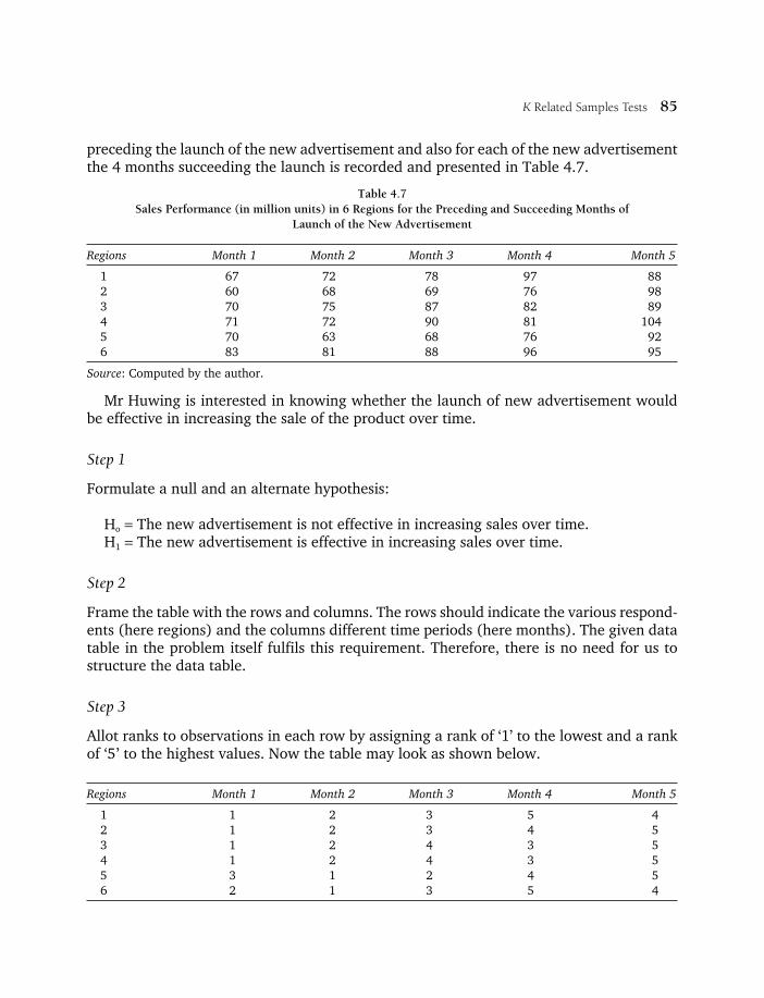
K Related Samples Tests 85
preceding the launch of the new advertisement and also for each of the new advertisement the 4 months succeeding the launch is recorded and presented in Table 4.7.
Table 4.7Sales Performance (in million units) in 6 Regions for the Preceding and Succeeding Months of
Launch of the New Advertisement
Regions Month 1 Month 2 Month 3 Month 4 Month 5
1 67 72 78 97 882 60 68 69 76 983 70 75 87 82 894 71 72 90 81 1045 70 63 68 76 926 83 81 88 96 95
Source: Computed by the author.
Mr Huwing is interested in knowing whether the launch of new advertisement would be effective in increasing the sale of the product over time.
Step 1
Formulate a null and an alternate hypothesis:
Ho = The new advertisement is not effective in increasing sales over time.H1 = The new advertisement is effective in increasing sales over time.
Step 2
Frame the table with the rows and columns. The rows should indicate the various respond-ents (here regions) and the columns different time periods (here months). The given data table in the problem itself fulfils this requirement. Therefore, there is no need for us to structure the data table.
Step 3
Allot ranks to observations in each row by assigning a rank of ‘1’ to the lowest and a rank of ‘5’ to the highest values. Now the table may look as shown below.
Regions Month 1 Month 2 Month 3 Month 4 Month 5
1 1 2 3 5 42 1 2 3 4 53 1 2 4 3 54 1 2 4 3 55 3 1 2 4 56 2 1 3 5 4

86 Data Analysis in Business Research
Step 4
Sum the ranks for each column and denote them as R1, R2, and so on.
R1 = 9; R2 = 10; R3 = 19; R4 = 24; R5 = 28
Step 5
Multiply each of R1, R2 and so on, by constants of 1, 2, 3….k, respectively and sum them together. Call the sum P.
P = (1 × 9) + (2 × 10) + (3 × 19) + (4 × 24) + (5 × 28) = 9 + 20 + 57 + 96 + 140 = 322
Step 6
Compare the calculated P with the critical P value by referring to Table 16 in the Appendix for k = 5 and n = 6.
For this illustration, the critical P is found as 29 for 5 per cent level of significance.
Step 7
Make a decision. Since the calculated P value of 322 is greater than critical P value of 29, the null hypothesis is rejected in favour of H1. Therefore, it is concluded that the new advertisement launched using celebrity spokesperson is effective in increasing the sale of the product over time.
Page’s Test for Large Sample
The critical values for Page’s test is found for the maximum k of 6 and n of 20. When ‘k’ and/or ‘n’ go beyond the table range, we have to follow the following procedure.
1. Calculate population mean (m)
μ = nk (k + 1)2/4
2. Calculate standard deviation (σ)
σ = + −nk k k2 21 1 144( )( )/

K Related Samples Tests 87
3. Find out the critical value by using the following formula and identify the Z value from the standard normal table for right-hand tail, and compare them for making decisions.
Critical region Z = μ + σ Z α + ½
In all these above cases, n = Number of rows
k = Number of columns α = Level of significance, usually 1.64 at 5 per cent level of significance for a
single-tailed test ½ = correction factor
Example: Suppose, k = 7 and n = 40, then
μ = nk (k + 1)2/4 = 40 × 7 (7 + 1)2/4 = 280 (16) = 4480
σ = + −nk k k2 21 1 144( )( )/
σ = × + −( ) ( )( )/40 7 7 1 7 1 1442 2
= 454.9
Critical region Z = μ + σ Z α + ½
= 4480 + 454.9 × 1.64 + ½ (Please note that Z α indicate the value of Z at 5 per cent level of significance for a right-tailed test, which is always1.64.)
= 4480 + 746.03 + ½ = 5226.53
If the calculated P value is greater than the critical P value of 5226.53, the null hypothesis will be rejected.
MATCH TEST FOR ORDERED ALTERNATIVES
This test is similar to the Neave–Worthington Ordinary Match test discussed earlier with the only exception that it is for ordered alternatives. In fact, this Match Test for Ordered Alternatives (MTOA) is considered to possess very respectable power (Neave and

88 Data Analysis in Business Research
Worthington, 1908: 295). The only difference is that in the case of the Neave–Worthington Match Test, we considered the preceding row’s values in different columns as reference points for finding out the matches and near matches in the succeeding rows of a data set. However, MTOA is slightly different because the ranks in each row are compared with a set of ‘predicted’ ranks to support the alternate hypothesis. Usually, the predicted ranks will be in an ascending order of 1, 2, 3…k.
Requirements
1. Variables should be measurable on the ordinal scale. In case variables are measured on interval scale, they have to be combined into ranks first.
2. Number of rows and columns can be any.3. Each row should have assigned ranks for all the columns.4. There should be strong theoretical or empirical or practical evidence that the column
values increase as one moves from left to right.
Advantages
It possesses good power. The critical value for this test statistic is independent of the number of treatments (columns).
Procedure
1. Form a null and an alternate hypothesis. The null hypothesis may be that the ‘k’ treatments (columns) have identical ranking pattern. The alternative hypothesis is that the ‘k’ treatments (columns) have a structured ranking pattern. It means that there will be an increasing or decreasing trend as we move from left to right in the data table.
2. Form a data table with rows indicating different respondents or sample objects and columns indicating the different treatments or periods.
3. If the data are of interval type, they need to be converted to ranks first.4. Have a predicted rank set of 1, 2, 3…k on the upper part (top-most row) of the table,
which can be used for comparing the ranks in each row in the table for finding out the number of matches and near matches.
5. Determine M1 and M2 which are the total number of matches and near matches, respectively. This can be found out by comparing ranks in each row against the predicted rank set written in the upper part of the table.
M1 = Total number of matches M2 = M1 + ½ (number of near matches)

K Related Samples Tests 89
A ‘near match’ exists if the difference between the rank in a predicted set and data set in the table differ by one and one only.
6. Find out the critical M1 and M2 values by referring to Tables 14 and 15, respectively in the Appendix. Here, the critical values are given for any number of columns (ks) and number of rows (ns) for 1 per cent and 5 per cent levels of significance. However, the critical values for M2 are restricted to a maximum k of 6 only.
7. Compare the calculated M1 and M2 values with the critical M1 and M2 values, and decide. If the calculated M1 and M2 values are ≥ the critical M1 and M2 values for the chosen level of significance, then reject the null hypothesis in favour of the alternate hypothesis.
Illustration
Let us go back to the data set given for the illustration in the Page’s Test section, which determines the effectiveness of the new advertisement launch on the sale of its product. For the sake of convenience, the data set comprising the ranks assigned to different months for each region is presented here. Apply MTOA to find out whether the new advertisement programme featuring a celebrity spokesperson is effective in increasing the sales over a period.
Region Month 1 Month 2 Month 3 Month 4 Month 5
1 1 2 3 5 42 1 2 3 4 53 1 2 4 3 54 1 2 4 3 55 3 1 2 4 56 2 1 3 5 4
Step 1
Form a null and an alternate hypothesis:
Ho = The new advertisement programme does not increase the sales of the product over months.
Ha = The new advertisement programme increases the sale of the product over months.
Step 2
Form a data table and ensure that all the rows have assigned ranks to all the columns. Here we have the data set which itself consists of ranks assigned for different columns. Therefore, nothing to worry.

90 Data Analysis in Business Research
Step 3
Prepare a data table such that you have the predicted rank set in the upper part of the column section of the table and call it ‘reference row’. This can be used for comparing ranks in each row of the main table for finding out M1 and M2. The data table, now, will appear as follows:
Predicted Ranks (Reference Row)
1 2 3 4 5
Regions Month 1 Month 2 Month 3 Month 4 Month 5
R1 1 2 3 5 4R2 1 2 3 4 5R3 1 2 4 3 5R4 1 2 4 3 5R5 3 1 2 4 5R6 2 1 3 5 4
Step 4
Compute M1 and M2. A detailed description on the concept and calculation of ‘matches’ is presented in the section on Neave–Worthington Match Test in the chapter.
M1 = The number of matches found between the ranks of the predicted set and the ranks of each row. Therefore, the number of matches for
Row 1 = 3Row 2 = 5Row 3 = 3Row 4 = 3Row 5 = 2Row 6 = 1
∴ M1 = 17
M2 = The number of near matches found between the ranks of the predicted set and ranks of each row, this time counting the number of times they differ by 1.
Row 1 = 2Row 2 = 0Row 3 = 2Row 4 = 2

K Related Samples Tests 91
Row 5 = 2Row 6 = 4
∴ Total near matches = 12.∴ M2 = M1 + ½ (number of total near matches) = 17 + ½ (12) = 17 + 6 = 23
Step 5
Find out critical values for M1 and M2 by referring to Tables 14 and 15, respectively in the Appendix.
For M1, the critical value for k = 5 and n = 6 at 5 per cent level of significance is = 11.For M2, the critical value for k = 5 and n = 6 at 5 per cent level of significance is = 15.
Step 6
Compare the calculated and critical M1 and M2 values and make a decision: Here, the calculated M1 value of 17 is ≥ critical value of 11. This gives the support that the ranks of the observed data follow the predicted order, thus rejecting the null hypothesis.
Similarly, the calculated M2 statistic of 23 is also ≥ than the critical value of 15, providing additional evidence in support of the alternate hypothesis. Hence we conclude that the new advertisement launch indeed increases the sale of the product over time in the predicted order. Is it not interesting to see that Page’s test results and Match test results are similar? Of course, you have many alternative tools available to test a similar situation. In most cases, it happens to be so. Just like you have different routes to reach a particular destination, these different techniques which share almost similar statistical power enable you to reach the same conclusion too. It is for you to decide which one to use.

5K Independent Samples Tests
In this chapter we study there major analytical tools for testing the significant differences among 3 or more sample groups. These are Kruskal–Wallis One-Way ANOVA, Mood’s Extended Median and Terpstra-Jonckheere Tests. The Kruskal–Wallis One-Way ANOVA is the nonparametric equivalent of the parametric One-Way ANOVA and is useful to check the mean rank difference among 3 or more groups. The Mood’s Extended Median Test enables us to find out whether k-independent samples are drawn from the population with an equal median. Finally, the Terpstra-Jonckheere Test, which is similar to Kruskal–Wallis One-Way ANOVA enables us to find out which group is different from which other group in case of rejection of the null hypothesis.
KRUSKAL–WALLIS ONE-WAY ANOVA
This test is popularly known as KW One-Way ANOVA and is used for finding out whether 3 or more samples come from the same population or from identical populations with respect to averages. This test was developed by William H. Kruskal and W. Allen Wallis in 1952, and since then it has been popularly called Analysis of Variance by Ranks. Unlike the parametric ANOVA, this KW nonparametric one-way ANOVA does not require the fulfilment of assumptions of normal distribution, interval data and homogeneity of group variance. This test is a more flexible, convenient, easy-to-use and powerful technique similar to a normal one-way ANOVA.
Requirements
1. Ordinal or interval data.2. There should preferably be at least 5 samples in each group.3. The sample size need not be equal for different groups.

K Independent Samples Tests 93
4. The logic of the KW Test is akin to that of the Mann–Whitney U Test as both the tests are based on ranked data. As in the Mann–Whitney U Test, in the KW Test we have to simply combine data to a group and array the scores from lowest to highest.
Advantage
1. This test is very flexible, as it also takes into account those groups with sample observations of less than or equal to 5, even though the prescribed number of observations in a group is 5.
2. It is as powerful as the parametric one-way ANOVA.
Procedure
1. Formulate a null hypothesis of no difference in the attribute (variable) measured among the groups.
2. Combine all the sample observations into 1 group.3. Arrange the observations from low value to high value.4. Assign a rank of ‘1’ to the observation of the lowest value, a rank of ‘2’ to the observation
of the next higher value, and so on. In case of ties, average the ranks and assign them to the tied observations. For example, in an ascending array of 5, 7, 9, 9, 9 and 12, the ranking distribution will be 1, 2, 4, 4, 4 and 6, respectively. That is, after rank ‘2’ we count 3, 4, 5 for observations with similar values of 9. Hence, the average of these ranks would be
3 4 53
123
4+ +
= =
5. Rearrange the data table in such a way that you have only the ranks of the respective observations for each sample group.
6. Sum up ranks for each group.7. Find out the H statistic by using the following formula.
HN n
R
nNj
i
k
=+
− +−∑12
13 1
2
11( )( )
where Rj = Sum of ranks in the jth sample. N = Total number of observations in all the groups put together. ni = Number of observations in the ith sample.

94 Data Analysis in Business Research
8. Compare the H value with the critical value found in Table 20 in the Appendix (for sample size 5 or less in all the groups). In case of a large sample size (sample size of > 5) in all groups, you can find the critical value by referring to Table 1 in the Appendix for k–1 degrees of freedom for a large sample.
9. Make a decision. If the computed ‘H’ value is greater than the critical value, reject the null hypothesis of no difference.
Illustration
Prof. Sastry wanted to test the difference between the mileage of 3 brands of cars that is, Maruti Zen, Hyundai Santro and Tata Indica in the small size segment. For this purpose he conveniently approached the faculty colleagues of his institution who owned any one of these brands. Prof. Sastry collected information about the mileage per litre in respect of the said brands from 12 of his colleagues which is reported in Table 5.1.
Table 5.1Mileage (per litre of petrol) of 3 Brands of Cars
Maruti Zen Hyundai Santro Tata Indica
17 11 9 11 10 11 16 9 9 15 13 15
Source: Computed by the author.
Find out whether any significant difference exists among the 3 brands of cars as far as mileage is concerned.
Step 1
Formulate a null and an alternate hypothesis:
H0 = The average mileage is the same for different brands of cars.H1 = There is a significant difference in the average mileage of cars among the brands.
Step 2
Arrange the observations from low to high values by combining all the sample observations into a single group. Here, it will be 9, 9, 9, 10, 11, 11, 11, 13, 15, 15, 16 and 17. Therefore, the ranks for these values will be 2, 2, 2, 4, 6, 6, 6, 8, 9.5, 9.5, 11 and 12, respectively. Please note that the ranks for the tied values are allotted in the same way as explained in procedure 4.

K Independent Samples Tests 95
Step 3
Rearrange the data table so that it contains only the ranks instead of the actual data.
Maruti Zen Hyundai Santro Tata Indica
12 6 2 6 4 611 2 29.5 89.5
Step 4
Total the ranks for each group and indicate them as R. Here it would be,
Maruti Zen : 12 + 6 + 11 + 9.5 + 9.5 = 48Hyundai Santro : 6 + 4 + 2 + 8 = 20Tata Indica : 2 + 6 + 2 = 10
Step 5
Apply the H statistic formula for finding out Kruskal–Wallis statistic
HN n
R
nNj
i
k
=+
− +−∑12
13 1
2
11( )( )
H = + +
⎡
⎣⎢
⎤
⎦⎥ − +
1212 13
485
204
103
3 12 12 2 2
( )( ) ( ) ( )
( )
H = + +⎡
⎣⎢⎤⎦⎥−
12156
23045
4004
1003
39
= 0.077 [460.8 + 100 + 33.3] – 39 = 0.077 [594.1] – 39 = 45.74 – 39 H = 6.74
Step 6
Compare the H value with the critical value. Please remember that we have to refer to critical value in Table 20 in the Appendix if the number of cases in each of the groups is 5 or less. In this way, the critical value by referring to Table 20 when the ns are 5, 4 and 3 is = 5.63

96 Data Analysis in Business Research
for 5 per cent level of significance (‘p’ value found in the last column of Table 20 in the Appendix is 0.049, which is definitely less than 5 per cent level of significance).
Step 7
Make a decision. Since the calculated H value of 6.74 is greater than the critical H value of 5.63 we reject the null hypothesis of no difference in the average mileage performance among different brands of cars. Therefore, we conclude that at least 1 brand of car is sig-nificantly different with respect to average mileage per litre of petrol.
Correction Factor
Some authors (Neave and Worthington, 1998 and Siegel, 1956), however recommend that correction factors may be introduced when ties occur between 2 or more observational scores. They contend that when a large number of ties occur, the value of H should be divided by ‘C’ which is nothing but the correction factor so as to give H∗ which is approximately χ2 distributed with (k–1) degree of freedom. The ‘C’ is calculated as below.
Ct t
N N= −
−−∑∑11
3
2( )
where t = Number of ties for a given tied value N = Total number of observations
Example
By using the data table of mileage performance of different types of cars as shown earlier we find that the observed mileage scores 9, 11 and 15 occur 3, 3 and 2 times respectively. If we prepare a table to calculate the correction factor, then it will be easily understood.
Observations t t3
9 3 2711 3 2715 2 8
∑t = 8 ∑t3 = 62
Ct t
N N= −
−−∑∑11
3
2( )
=−
⎡⎣ ⎤⎦ −
⎡
⎣⎢⎢
⎤
⎦⎥⎥
162 8
12 12 12( )

K Independent Samples Tests 97
∴= −
−⎡
⎣⎢
⎤
⎦⎥1
5412 144 1[ ]
= − ⎡
⎣⎢⎤⎦⎥
154
1716
= 1 – 0.031
= 0.969
Therefore, the corrected value of H∗ will be H∗ = HC
=
6 740 969
..
( )ascalculatedearlier
= 6.95
We find that the original H value of 6.74 and the corrected value of H∗ of 6.95 are not very far from each other. Nevertheless, the null hypothesis is rejected at the same level of significance. Hence, using the correction factor (H∗) is insignificant unless we find that the number of ties is huge in the given data set. You will be surprised to learn that the effect of the correction factor is negligible in spite of the fact that 8 out of 12 observations (75 per cent) in the car example are involved in ties. However, we can use the correction factor for accurate results.
Example for a Large Sample
Karunya Institute of Technology and Sciences is a deemed university located in Coimbatore, India. Before the classes commence each day, it is customary that the students attend morning assembly sessions wherein the faculty members, students, non-teaching staff and the guest speakers from outside share their thoughts. The time allotted for such sharing is 10 minutes. Over a month, the approximate time taken (in minutes) by speakers from these different segments was recorded and is presented in Table 5.2.
Table 5.2 Distribution of Time Taken (in minutes) for Sharing of Morning Thoughts by Speakers of Different Segments
Segment 1Faculty
Segment 2 Non-teaching Staff
Segment 3Students
Segment 4 Guest Speakers
11 10 7 1513 9 8 2016 8 6 1212 11 7 11
(Table 5.2 continued)

98 Data Analysis in Business Research
Segment 1Faculty
Segment 2 Non-teaching Staff
Segment 3Students
Segment 4 Guest Speakers
4 12 96 10 13
10151314
Source: Computed by the author.
Examine whether the average time taken by the speakers in a particular segment is significantly different from the rest.
Step 1
Formulate a null and an alternate hypothesis:
H0 = There is no difference in the average time taken by speakers from different segments.H1 = There is a significant difference in the average time taken by speakers from different
segments.
Step 2
Arrange all the observations in an ascending order.
4, 6, 6, 7, 7, 8, 8, 9, 9, 10, 10, 10, 11, 11, 11, 12, 12, 12, 13, 13, 13, 14, 15, 15, 16, 20
Step 3
Arrange the data table so that it contains only the ranks of the observed data.
Segment 1Faculty
Segment 2Non-teaching Staff
Segment 3 Students
Segment 4 Guest Speakers
14 11 4.5 23.520 8.5 6.5 2625 6.5 2.5 1717 14 4.5 141 17 8.52.5 11 20
1123.52022
(Table 5.2 continued)

K Independent Samples Tests 99
Step 4
Total the rank for each segment and indicate it as ‘R’. Hence,
Faculty : 14 + 20 + 25 + 17 + 1 + 2.5 + 11 + 23.5 + 20 + 22 = 156Non-teaching Staff : 11 + 8.5 + 6.5 + 14 + 17 + 11 = 68Students : 4.5 + 6.5 + 2.5 + 4.5 + 8.5 + 20 = 46.5Guests : 23.5 + 26 + 17 + 14 = 80.5
Step 5
Calculate the H statistic.
H
N N
R
nNj
ii
k
=+
− +=∑12
13 1
2
1( )( )
H =
++ + +
⎡
⎣⎢
⎤
⎦⎥ − +
1212 26 1
15610
686
46 56
80 54
3 26 12 2 2 2
( )( ) ( ) ( . ) ( . )
( ))
H = + + +⎡
⎣⎢⎤⎦⎥−
12702
2433610
46246
2162 256
6480 254
81. .
= 0.017 [2433.6 + 770.67 + 360.37 + 1620] – 81 = 0.017 [5184.6] – 81 = 88.14 – 81 H = 7.14
Step 6
Find out the critical H value. Since this is a case of large sample wherein the number of observations in any single group exceeds 5, we cannot use the Kruskal–Wallis table shown in Table 20 in the Appendix. As has been described under the head ‘procedures’ at the beginning of this chapter, for large samples we have to use the χ2 table (Table 1 inthe Appendix) for k–1 degrees of freedom which in this case is (4 groups – 1) = 3. The table value is 7.81 for 5 per cent level of significance.
Step 7
Make a decision. Since the calculated H value 7.14 is less than the table value of 7.81, it is evident that the null hypothesis is confirmed. Hence there is no significant difference

100 Data Analysis in Business Research
in the average time taken for delivering the morning thoughts in the college assembly by speakers of different segments.
Note: Perhaps you may wonder that the time taken by the students segment in most cases (that is, 5 out of 6) is less than 10 minutes and it is quite natural for youto raise your eyebrows and ask, ‘How come this Kruskal–Wallis Test has yieldeda result of no significant difference among different segments?’ There might be 2 reasons; one is that the test results might indicate that the average time taken by students in that particular month might be purely due to chance (random) factor.
The second reason might be due to the presence of large number of ties of different groups in the actual data scores combined together. You may find that upon arranging theobservations (scores) in an ascending order, excepting for 4, that is, 4, 14, 16 and 20, all the remaining 22 observations are involved in ties. This amounts to 22/26 × 100 = 84.6 per cent of ties in the sample data, which is really a matter of concern. Therefore what will you do? You have already learnt that a correction factor may be introduced for a data set that contains a large number of ties. It is relevant that you endeavour the use of correction factor in your calculation of the Kruskal–Wallis H∗ (of course, by following the same procedures given for small sample case), as shown below.
Step 1
Prepare a table to calculate the correction factor for identifying the number of ties involved for different observations.
Observations t t3
6 2 87 2 88 2 89 2 8
10 3 2711 3 2712 3 2713 3 2715 2 8
∑t = 22 ∑t3 = 148
Step 2
Calculate ‘C’ the correction factor.

K Independent Samples Tests 101
Ct t
N N= −
−−
⎡
⎣⎢⎢
⎤
⎦⎥⎥
∑∑11
3
2( )
C = −−−
⎡
⎣⎢
⎤
⎦⎥1
148 2226 26 12( )
C = −−
⎡
⎣⎢
⎤
⎦⎥1
12626 676 1( )
C = −−
⎡
⎣⎢
⎤
⎦⎥1
12626 676 1( )
C = 1 – 0.0072 = 0.99
C = 0.99
Step 3
The corrected value of KW–H∗ is
HHC
∗ =
H∗ =
7 140 99..
H∗ = 7.21
Wow! The corrected KW statistic (H∗) of 7.21 is almost close to the uncorrected H value of 7.14, which indicates that there is still no statistical evidence to reject the null hypoth-esis of no difference in the average time taken by speakers of different segments in sharing their thoughts in the morning assembly.
MOOD’S EXTENDED MEDIAN TEST
This test, introduced by Mood in 1950, is used to find out the significant difference in theattribute measured with respect to 3 or more groups. In other words, by using Mood’s Median Test we can find out whether k independent samples or groups are drawn from the same population or populations with equal medians. We should remember that the test of difference is found out by using median and not by using mean.

102 Data Analysis in Business Research
Requirements
1. There should be ordinal or interval scaled measurement variables.2. The sample size need not be equal for different groups. Therefore, one group may have
10 samples or observations while the other groups may have just 2 or 3 observations.
Advantages
1. Compared to Kruskal–Wallis Test which is also used for finding out the difference between more than 2 groups, the Mood’s Median Test is very easy to execute when the sample sizes are large.
2. This test is convenient to use when there are more number of ties in the data.
Procedure
1. Combine the values of all observations from all the groups in an ascending order. 2. Find the median for all the ‘k’ samples combined. Call it overall median.3. Count the number of observations whose scores are above and below the overall
median.4. Prepare separately a 2×k contingency table with the counts made in step 3, where
‘k’ stands for number of treatments or conditions. 5. Calculate the chi-square value for the table.6. If the calculated chi-square value is greater than the critical chi-square value obtained
from Table 1 in the Appendix then reject the null hypothesis and accept the alternate hypothesis.
Illustration
Prof. Kokkariwala was considering how to improve the performance of his stu-dents in the course on Research Methods. On earlier occasions, he had tried out several teaching methods but was confused about the feasibility of a particular method for im-proving the students’ performance. Hence he decided to experiment with student volunteers who opted to learn the subject through one of the following methods: case method of learning, conventional method of lecturing, a combination of both case and lecturing methods, and Socratic (learning through questioning) method. There were 60 students in the class and 32 students volunteered to take part in the experiment, with 10 of them opting for the case method, 11 for the lecturing method of learning, 8 for the combination of lecturing and case, and 3 students opted for Socratic learning. The experiment was conducted for a term of 3 months after which the test was administered to all and their

K Independent Samples Tests 103
performance scores were computed. During the experiment, Prof. Kokkariwala also ensured that the students in the different learning methods did not interact with each other so as to eliminate the influence of experimental errors that would impinge the experiment of results. Table 5.3 presents the scores.
Table 5.3 Scores Obtained by Students of the Research Methodology Course under Various Learning Methods
Case Method Lecture MethodCombined Method (Case and Lecture)
Socratic Method
48 50 70 6779 53 65 6676 62 42 5643 71 5381 42 5769 38 6259 79 6340 67 5488 4877 56
60
Source: Computed by the author.
Prof. Kokkariwala wants to test the hypothesis that the students’ performance in the Research Methods course will vary according to different learning methods.
Step 1
Combine the values of all the observations in an ascending order: 38, 40, 42, 42, 43, 48, 48, 50, 53, 53, 54, 56, 56, 57, 59, 60, 62, 62, 63, 65, 66, 67, 67, 69, 70, 71, 75, 77, 79, 79, 81, 88.
Step 2
Find the overall median for the whole set of observations. Since N = 32 observations altogether, the overall median is the average of 16th and 17th values. Hence, the overall median = 60 + 62/2 = 61.
Step 3
For each sample count the number of observations that lie above and below the overall median. Based on this the following table is made. The observations whose values are above the overall median are indicated with a ‘+’ sign while the observations with values less than the overall median are identified with a ‘–’ sign.

104 Data Analysis in Business Research
Case Method Lecture Method Combined Method (Case & Lecture) Socratic Method
– – + ++ – + ++ + – –– + –+ – –+ – +– + +– + –+ –+ –
–Total (+) 6 4 4 2Total (–) 4 7 4 1
Step 4
Construct a 2×k contingency table based on the counts made in Step 3.
Case Method
Lecture Method
Combined Method
Socratic Method Total
Number above the overall median (+ signs)
6 4 4 2 16
Number below the overall median (–)
4 7 4 1 16
Total 10 11 8 3 32
Step 5
Perform a Chi-Square Test for the contingency table framed in step 4. We have already learnt in Chapter 2 that chi-square is calculated as
( )Observed frequency Expected frequency
Expected frequency
−∑ 2
Wherein the expected frequencies are calculated by using the following formula:
E ected frequency forrow totalof the column totalof therespectxp
=×iivecell respectivecell
grand totalof thecontingency tablea partiicular cell
In this illustration, there are 8 cells for the contingency table. (Note that the total row and total column will not be considered for counting the number of cells for which we

K Independent Samples Tests 105
need to compute expected frequencies.) For example, for cell 1 of the contingency table in step 4, the observed frequency is 6 while the expected frequency will be 10 × 16/32 =160/32 = 5. For cell 2, the observed frequency is 4 while its expected frequency will be 11 × 16/32 = 5.5. In this way the expected frequency for
cell38 16
324,
×=
cell4
3 1632
1 5, .×
=
cell5
10 1632
5,×
=
cell6
11 1632
5 5, .×
=
cell7
8 1632
4,×
=
cell8
3 1632
1 5, .×
=
Let us frame a table to facilitate easy calculation of the chi-square statistic as shown below:
ObservedFrequency (O)
Expected Frequency (E)
(O–E) (O–E)2 (O–E)2/E
6 5 1 1.0 0.204 5.5 –1.5 2.25 0.414 4 0 0 02 1.5 0.5 0.25 0.174 5 –1 1.0 0.207 5.5 1.5 2.25 0.414 4 0 0 01 1.5 –0.5 0.25 0.17
∑ = 1.56
Therefore, the calculated chi-square = 1.56.
Step 6
Identify the critical value from the chi-square distribution by using Table 1 in the Appendix for (k – 1) degrees of freedom, where k = number of groups. Hence, the degrees of freedom for this case = (4 – 1) = 3. We find that the critical chi-square value for 3 degrees of freedom at 5 per cent level of significance is equal to 7.815.

106 Data Analysis in Business Research
Step 7
Make a decision by comparing the calculated chi-square statistic and the critical chi-square value. If the calculated chi-square value is greater than the critical chi-square value then we reject the null hypothesis of no difference among the sample groups, otherwise we conclude that there is a statistical evidence to support the alternative hypothesis that there are significant differences in the students’ performance in different learning methods. In thepresent case, we see that the calculated chi-square value of 1.56 is less than the critical chi-square value of 7.815. Thus, we conclude that students’ performance is not influenced bydifferent learning methods. Therefore, our submission to prof. Kokkariwala is that the students’performance in the Research Methods course is independent of different learning methods.
TERPSTRA-JONCKHEERE TEST FOR ORDERED ALTERNATIVES
Popularly known as Jonckheere Test, it is very useful when one wants to test the ordered pattern to medians of the groups compared (Field, 2005). Tests such as Kruskal–Wallis One-Way ANOVA and Moods Median simply tell us whether there is any significant difference among the average ranks of different groups. If a null hypothesis of no difference is rejected, we simply conclude that the groups do differ with regard to the median of the attribute measured. To find out which group is different from which other group (s), we perform a multiple comparison like Dunn’s Multiple Comparison Test (described in Chapter 8). Nonetheless, such multiple comparison tests too, simply portray the existence of difference between any 2 groups. That is all. But many a times it becomes necessary to test an alternative hypothesis specifically indicating the order or direction of any differences that may exist among the sample medians, like H1: φ1 > φ2 > φ3 ……> φn, where φ indicates group median. For example, let us presume that the TV advertisement is more effective (ETA) than print advertising (advertisement through newspaper, magazines, and so on–ENA), which in turn is more effective than advertisement through radio (ERA). The null and alternate hypothesis in this case will be:
H0 : ERA = ENA = ETA
H1 : ERA < ENA < ETA
While the null hypothesis indicates the presence of no difference in the effectiveness of different advertisement media, the alternate hypothesis (H1) indicates a more specific statement of the relative effectiveness of advertisements in different media rather than simply saying, ERA ≠ ENA ≠ ETA. Such a type of specific statement is known as an ‘ordered alternative hypothesis’ and the testing process is quite different from the general alternate hypothesis of no difference among the groups. T. J. Terpstra (1952) and A. R. Jonckheere (1954) have propounded the procedures for testing the ‘k’ independent samples with an ordered alternative hypothesis.

K Independent Samples Tests 107
Requirements
1. Ordinal or interval variables.2. The sample size in each group should be preferably equal, even though violation of
this is not a serious threat. 3. The samples should be drawn from independent populations. 4. It is always a 1-tailed test.
Advantages
1. This test checks the upward or the downward trend in the medians of the groups compared.
2. The alternative hypothesis can be tested more specifically rather than simply saying that the null hypothesis is rejected.
Procedure
1. Form a null hypothesis of no difference between the treatments and the alternate hypothesis of an orderly occurrence of a particular event.
2. Rank order all the scores. This can be made easy by drawing a straight line and indi-cating the position of each observation on the scale along with specifying the name ofappropriate sample or group on the top line. For example, consider the following table.
A B C
15 60 9025 20 6035 65 6590 40 7015 70 62
95 8095
We have 5 observations in group A, 6 in B and 7 in group C. The plotting of points on a scale for different observations becomes slightly ticklish when the ties occur for observations in different samples. In the above table, we have a total of 5 tied observa-tions (4 tied observations for groups B and C for a score of 60, 65, 70 and 95, and another tied score of 90 for groups A and C).
Now, we should be very cautious in plotting the tied observations. How to do it? So long as the ties occur between observations in a single group or sample, it is not a prob-lem. Such cases will be simply exhibited by plotting them one over the other as you see in the line graph for the tied values of 15 in group A and 60 in groups B and C.

108 Data Analysis in Business Research
The same procedure is followed when we have ties occurring between observa-tions in different samples, but with the addition of adding a score of ½ to such cases.
3. Calculate the U statistic for each pair of groups. If there are 3 groups, then 3 U statistic [k (k – 1)/2], where k is the number of groups, which is [3 × (3 – 1)/2] as below:
(a) UBA = number of AB pairs with B < A (b) UCA = number of AC pairs with C < A (c) UCB = number of BC pairs with C < B A small U statistic establishes the alternate hypothesis.
4. Calculate Terpstra-Jonckheere W statistic.
W = UBA + UCA + UCB
5. Find out the critical value by referring to Table 17 in the Appendix for the appropriate ‘k’ values and ‘n’ sample sizes.
In case of large samples calculate the critical value by using the following formula.
Critical W value = μ 2 σ ½
where
N niμ =−∑2 2
4
Z = Corresponding (right-hand tail) normal distribution value
½ = Correction factor
σ =+ − +∑N N n ni i
2 22 3 2 3
72
( ) ( )
where N = Total number of observations combined for all the groups n = Number of observation in a single group
6. Make a decision by comparing the calculated W and critical W values. If the calcu-lated W is less than or equal to the critical value (please note that the calculated W should be less than the critical value and not the other way round as it is commonly used), then reject the null hypothesis. In other words, the smaller the value of the calculated W, the more the probability of supporting the alternate hypothesis (H1).

K Independent Samples Tests 109
Illustration
A recent sport report released by PCB (Pakistan Cricket Board) elicited an interesting finding that was based on a study conducted by Pakistan Sports Federation on 22 cricket players and their performance under 3 different coaches over a period of 15 months. The performance rating of the players on the basis of runs scored per match in all the one-day international matches held during the specified period, trained by 3 different coaches are presented in the following data table (Table 5.4).
Table 5.4Runs Scored (per match) in the One-Day International (ODI) Matches by
Players Trained by 3 Different Coaches
DomesticCoach (runs scored)
InternationalCoach
(runs scored)
Professional Coach
(runs scored)
22 32 2927 29 3635 40 4924 47 3931 39 5419 52 56
44 604955
Source: Computed by the author.
Do we have the statistical evidence to conclude that the average runs scored by the players increased as we progressed from those trained by a domestic coach to those trained by an international coach and finally to those trained by a professional coach?
Step 1
Form a null and an alternate hypothesis:
Ho = There is no difference in the runs scored by players trained by different coaches.H1 = The runs scored by players increase progressively from domestic to professional
coach.
Step 2
Rank order all the scores by drawing a line graph. As described earlier, in the case of tied observations (whether they occur in the same group or different groups) their groups need to be specified one over the other. The following line graph exhibits this.

110 Data Analysis in Business Research
Step 3
Calculate the U statistic for each pair of groups. Here, we have 3 groups of training given. There would be 3 pairs [3 × (3 – 1)/2] to compare with. Let us, therefore, calculate UID, UPD and UPI
where UID = Number of DI pairs with I < D UPD = Number of DP pairs with P < D UPI = Number of IP pairs with P < I∴ All possible pairs where I < D = 3All possible pairs where P < D = 2and all possible pairs where P < I = ½ + 1 + 1 + 1 + 1 + 1 + 1 + ½ + 1 + 1 + 1 + 1 + 1 + 1 = 18
Step 4
Calculate the Terpstra-Jonckheere W statistic.
W = UID + UPD + UPI
= 3 + 2 + 18 = 23
Step 5
Find out the W statistic by referring to Table 17 in the Appendix. The critical value of W at 5 per cent level of significance for k = 3; n1 = 6, n2 = 7 and n3 = 9 is found to be 52.
Step 6
Make a decision by comparing the calculated W and critical W.Since the calculated W of 23 is less than the critical W of 52 there is a strong evidence to support our claim that the performance of cricket players increased as we moved from training by a domestic to a professional coach.

6Measures of Correlation and Association
In this chapter various measures of correlation and association are presented. The Spearman’s Rank Correlation Coefficient is used for measuring the relationship between 2 ordinal variables. While phi-correlation coefficient is used for testing the degree of association between 2 dichotomous variables, the Contingency Coefficient is useful to find out the degree of association between 2 nominal variables, each with ‘n’ number of categories. The Cramer’s V coefficient is an extension of Contingency Coefficient and is used to analyse the relationship between 2 nominal variables with ‘n’ number of categories, with an upper correlation coefficient of 1. The Goodman–Kruskal Lambda measures the association between 2 variables that are measured on nominal scale—each variable with 2 or more categories—and is based on the assumptions of proportional reduction error. The Goodman–Kruskal Gamma is used to find out the degree of relationship between 2 ordinal variables that are presented in a tabular form. The Somer’s d, as an extension of Gamma, is used for analysing the relationship between 2 ordinal variables with more number of tied pairs of cases. The Kendall’s Tau is effective to find out the relationship between 2 ordinalvariables when there is more number of ties in the data. The Kendall’s Tau-b measures the relationship between 2 ordinal variables with several categories and is recommended for a square-format contingency table where the number of rows and columns are equal. The Kendall’s Partial Rank Correlation Coefficient is effective to find out the relationship between 2 variables after controlling the effect of third variable. The Point Biserial Correlation analyses the relationship between 2 variables in which one is measured on nominal scale and the other on an interval scale. The high correlation coefficient measures the strength of relationship between 2 variables that are dichotomous and are presented in a 2×2 contingency table. The Cohen’s Kappa measures the degree of consistency in respect of ratings measured on a dichotomous scale. The Kendall’s Coefficient of Concordance, an extension to Friedman Two-Way ANOVA, indicates the degree of association among the variables’ ranking. The Mantel–Haenszel’s Chi-Square is yet another measure for finding out the degree of relationship between 2 sets of ranks.
SPEARMAN’S RANK CORRELATION COEFFICIENT
Spearman’s Rank Correlation Coefficient, also known as Spearman’s rho or ‘rs’ is a measure of degree of relationship between 2 ordinal variables. As one of the oldest techniques it was

112 Data Analysis in Business Research
propounded in 1904 by Charles Edwards Spearman, an English psychologist and statistician. Like the correlation coefficient, its value also ranges from ‘–1’ to ‘+1’. A value of ‘–1’ indicates a perfect negative relationship, a value ‘+1’ indicates a perfect positive relationship and a value of ‘0’ indicates no relationship at all. A positive sign means that if a respondent is ranked high in one attribute he or she will be ranked high in the other attribute also. A negative sign means the opposite. It should also be noted that if a respondent is ranked low in both attributes then also there exists a positive association. Spearman’s rho is effective when there are fewer ties. In simple words, Spearman’s rho measures the degree of agreement between 2 sets of ordinal data.
Requirements
The variables should be measured on oridinal scale. If the variables are measured on interval/ratio scale then they should be first converted into ranks.
Advantages
1. This test is useful when we have less number of tied ranks in the data set.2. This test is not influenced by outliers or extreme scores. Therefore, it does not pose
any threat to the findings of the study.3. Its statistical significance can be performed.
Procedure
1. State a null and an alternate hypothesis. The null hypothesis may be that there is no agreement between the ranks assigned by 2 methods or experts on ‘n’ objects. The alternate hypothesis may be that there is a significant agreement between the ranks assigned by 2 methods/experts on ‘n’ objects.
2. Convert the actual scores obtained into ranks for each of the 2 variables begin-ning with the rank of 1 (in case of tied scores, assign the average rank correspond-ing to those scores). If scores are given in ranks, then there is no need to convert them.
3. Determine the value of ‘D’ for each respondent. ‘D’ stands for the rank difference for each respondent on the attributes/judges’ ranking, that is, xi and yi. Therefore, d = xi – yi, where, xi and yi indicate the ranks allotted by the respective judges or ranks awarded by each of the respondent on each of the attributes.

Measures of Correlation and Association 113
4. Apply Spearman’s rho (rs) formula:
r
Dnx ns =− ∑
−1
61
2
2( )
where n = the number of objects ranked.
5. Calculate the critical value if the sample size is 30 or less. Consult Spearman’s test statistic Table 21 found in the Appendix. In case of a sample size being greater than 30 find out the critical value either through calculating critical ‘t’ or ‘z’.
Critical t
r nr
s
s
=−
−( )21 2
where rs = Spearman’s rho, n = number of respondents/objects being ranked. Or
Critical z r ns= −1
6. Compare the critical value and calculated value and make a decision.
(a) For sample size of 30 or less compare the calculated rs with critical Spearman statistic for the corresponding ‘n’ (which you have obtained from Table 21 in the Appendix). If the calculated rs is greater than the critical value then reject the null hypothesis of independence in ranking by 2 methods or experts.
(b) Use of critical ‘t’. The calculated ‘t’ value should be compared with critical ‘t’ value found in Table 22 in the Appendix for n – 2 degrees of freedom. If the calculated ‘t’ is larger than the critical ‘t’ value the null hypothesis will be rejected.
(c) In case of use of critical ‘z’ value, the null hypothesis will be rejected if the cal-culated ‘z’ is out side the critical ‘z’ of ± 1.96 for a 2-tailed test and ± 1.64 for a single-tailed test.
Illustration
Prof. Kudumba Sastry, Admission Coordinator for the MBA programme wants to measure the strength of relationship between students’ CAT (Common Admission Test) scores and their academic performance. For this purpose, he randomly chose 15 MBA students who were ranked from 1 to 15 based on the scores of the MBA entrance examination. The same 15 students were ranked again according to their overall percentage of marks obtained at the end of the programme. Prof. Sastry feels that the information in this regard will enable him to predict the academic performance of the students using the CAT score.

114 Data Analysis in Business Research
The following table (Table 6.1) exhibits the scores obtained by 15 MBA students in CAT exam and their end-semester examination.
Table 6.1Test Scores Obtained by Sample Students in the Entrance Exam and End-semester Exams
Student Entrance Examination Score End Semester Exam Score
A 85 84B 78 83C 55 57D 90 81E 79 79F 63 51G 88 75H 50 62I 74 54J 73 59K 66 61L 75 70M 82 64N 71 49O 84 63
Source: Computed by the author.
Step 1
State a null and an alternate hypothesis.
Ho: There is no agreement between ranks obtained by students in the entrance exam-ination and their academic performance.
Ha: There is a significant association between the ranks obtained by students in the entrance examination and their academic performance.
Step 2
Convert the actual scores into ranks.
The conversion of scores into ranks should be done for each variable separately.The results are depicted in the analysis Table 6.2.
Step 3
Find the difference in ranks obtained for entrance examination and academic performance scores. Call it ‘D’. This step too is depicted in the data analysis table.

Measures of Correlation and Association 115
Table 6.2Spearman’s rho Calculation for Ranks on Student’s Entrance Exam and Academic Performance
StudentEntrance Exam
Rank (xi)Academic Performance
Rank (yi)Difference
(D = xi – yi) D2
A 13 15 –2 4B 9 14 –5 25C 2 4 –2 4D 15 13 2 4E 10 12 –2 4F 3 2 1 1G 14 11 3 9H 1 7 –6 36I 7 3 4 16J 6 5 1 1K 4 6 –2 4L 8 10 –2 4M 11 9 2 4N 5 1 4 16O 12 8 4 16
ΣD2 = 148
Source: Computed by the author.
Step 4
Apply Spearman’s rho formula.
r
Dn ns =− ∑
−1
61
2
2(
rs =
− ×−
16 148
15 15 12( )
rs =
−1
8883360
rs = 1 – 0.26 rs = 0.74
This value of 0.74 reveals a strong positive association between the ranks on students’ CAT score and their academic performance.
Step 5
Compute the critical value. Since the sample size is less than 30 let us refer to Table 21 in the Appendix for finding out the critical value for n = 15. In this case it is found to be 0.442 at 5 per cent level of significance.

116 Data Analysis in Business Research
Step 6
Compare the calculated and critical values and make a decision.Since the calculated value of 0.74 is much higher than the critical Spearman statistic of
0.442, there is no statistical evidence to support the null hypothesis. Hence, it is concluded that there is a significant positive association between the ranks obtained by students in the CAT exam and their overall academic performance.
PHI-CORRELATION COEFFICIENT
This technique is very useful when we want to measure the strength of association be-tween the 2 variables that are dichotomous. Therefore, whenever we come across a 2 × 2 table (that is, a table with 2 rows and 2 columns), it is easier for us to assess the strength of the association between the 2 variables. In other words, once we have found out the significant association for variables in a 2 × 2 table using a chi-square statistic, we have to also measure the degree of association between these variables. Like correlation coefficient, a phi-correlation also ranges between –1 and +1 with a value of 0 indicating no relationship between the variables.
Requirements
1. Two variables both measured on a dichotomous scale.2. Significant chi-square value obtained for the distribution. That is, it serves no pur-
pose computing a phi-coefficient for a 2×2 contingency table with non-significant chi-square value.
Advantages
1. It is the only method available to find out the strength of association between 2 vari-ables measured on a dichotomous scale.
2. It is easy to calculate and interpret.3. The significance of phi-correlation can be tested.
Procedure
1. Form a null and an alternate hypothesis. The null hypothesis may be that the 2 vari-ables are independent while the alternate hypothesis may be that the 2 variables are associated.

Measures of Correlation and Association 117
2. Perform a chi-square analysis for the contingency table and ensure the acceptance of alternate hypothesis. In case of acceptance of null hypothesis, there is no need to compute phi-coefficient.
3. Apply phi-correlation coefficient formula to find out the strength of association. Once we have observed the significance of chi-square for the contingency table, then we can proceed with computing the phi-coefficient.
Φ =
xN
2
where Φ = phi, x2 = Chi-square value N = Number of samples
Illustration
The following is the data table (Table 6.3) depicting the eye colour and gender of the sample respondents. A total of 100 respondents comprising 55 men and 45 women were contacted and their eye colour was identified as either black or blue.
Step 1
Formulate a null and an alternate hypothesis:
Ho: There is no association between eye colour and gender of the respondents.Ha: Eye colour and gender of the respondents are associated.
Table 6.3
Eye Colour and Gender of the Sample Respondents
Eye Colour
Gender
Male Female Total
Black 45 7 52Blue 10 38 48Total 55 45 100
Source: Computed by the author.
Step 2
Find out the chi-square statistic for the data table and ensure that there exists a significant association between gender and eye colour. This requires us to calculate the chi-square

118 Data Analysis in Business Research
statistic by adopting the same procedures described in chapter 2, in this book. The chi-square value for the given data table is computed as follows:
Observed (O) Expected (E) (O–E) (O–E)2 (O–E)2/E
45 55 × 52/100 28.6 16.4 268.96 9.4010 55 × 48/100 26.4 –16.4 268.96 10.187 45 × 52/100 23.4 –16.4 268.96 11.49
38 45 × 48/100 21.6 16.4 268.96 12.45Σ = 43.52
The calculated chi-square statistic is 43.52 whereas the critical chi-square for 1 degree of freedom from Table 6 in the Appendix is 3.84 at 0.05 level of significance. Since the calculated chi-square statistic is greater than the critical chi-square value, we conclude that there is a significant association between the gender of the respondents and their eye colour.
Step 3
Compute phi-correlation coefficient by applying the formula. This is required to assess the degree or strength of association between eye colour and gender of the respondents.
Φ = =
xN
43.52100
2
Φ = 0 4352.
Φ = 0.66
The phi value of 0.66 indicates that there is a strong association between gender and colour of the eye, and this correlation is statistically significant.
Note
1. If the phi value (Φ) is squared, it represents the proportion of variance explained or shared between the 2 variables. For example, the (rΦ)2 for gender and eye colour is 0.43, which implies that 43 per cent of the variation in eye colour is explained by variation in gender (in a contingency table, the dependent variable is shown as a row variable).
2. The procedure described above is applicable when we have data collected from the sample. In case the data is collected from the entire population (and not from the sample), then the significance of rΦ is not an issue and therefore there is no need at

Measures of Correlation and Association 119
all to find out the chi-square statistic. In such a situation, a phi-coefficient can be computed straight away by using the following formula:
r
ad bca b c d a c b dphi =
−+ + + +( )( )( )( )
Where a, b, c and d represent cell frequencies in a 2×2 contingency table. Usually, the table is arranged as follows:
Variable X+ –
Variable Y + a b
– c d
The plus and minus signs indicate the presence and absence of a particular quality of the attribute. For example, for variable Y, a ‘+’ sign indicates black eye colour while a ‘–’ sign indicates blue eye colour. Similarly, cell ‘a’ in the table indicates those respondents who are male and have black eyes, and so on.
CONTINGENCY COEFFICIENT
This statistic is extremely useful when we want to find out the degree of relationship or association between 2 nominal variables, each with n number of categories. Thus the degree of association between 2 variables in a cross tabulation of r rows and c columns is deter-mined by a contingency coefficient. While phi-coefficient is ineffective for a contingency table where either rows or columns exceed 2, the contingency coefficient is robust in such a situation. It is not required that the categories in 2 variables should be arranged or ordered in a particular way. Therefore, as a symmetric measure one will get the same contingency coefficient value irrespective of how the categories are arranged in the rows and columns. The contingency table is also a mode of assessing not only the significance of dependence but also the degree of dependence of 1 variable (row variable) on the other variable (column variable) (shown along the columns) on the other variable (shown row wise) (Conover, 1980).
Requirements
1. Variables should be measured on a nominal scale. The number of categories for a particular variable is immaterial.

120 Data Analysis in Business Research
2. It is also required to compute the upper limit for contingency coefficient (a detailed description is made in the procedures section).
3. The significant association between different categories of 2 variables should be ascertained first through performance of a Chi-Square Test. If the chi-square result is insignificant, it is futile to compute the contingency coefficient.
Advantages
1. This is a sophisticated technique for measuring the degree of association when we have a contingency table of any number of rows and columns.
2. The significance of the contingency coefficient can be tested through chi-square distribution.
3. Two contingency coefficients can be compared with each other provided the tables are of the same size (same rows and columns).
4. There is no need to order the categories in a variable as the contingency coefficient will be the same irrespective of how the categories are arranged in rows and columns.
Procedure
1. Arrange the data in a c×r contingency table where c = number of columns and r = number of rows.
2. Find out the chi-square value for this contingency table so formulated (refer the section on two-sample chi-square described in Chapter 2 in this book) with respect to a detailed presentation on the method of calculating the chi-square value).
χ2
2
11
=−
==∑∑
( )O E
Eij ij
ijj
c
i
r
where O = Observed frequency in each cell of the contingency table. E = Expected frequency in each cell of the contingency table.
3. Apply the contingency coefficient formula.
C
N=
+χχ
2
2
where N = Total number of respondents.
4. Find out the upper limit for the contingency coefficient. Since the contingency coefficient will not have +1 as its upper limit when there is a perfect agreement, it

Measures of Correlation and Association 121
needs to be calculated based on a number of categories in the contingency table. The following points need to be considered:
(a) When the number of rows and the number of columns are equal in the contin-
gency table, the upper limit of 2 perfectly correlated variables is found out by applying the formula.
CC−1
where C = Either the number of columns or rows as both happen to be the same.
For example, for a 4 × 4 contingency table (that is, a 4 rows × 4 columns table) the upper limit of contingency coefficient
=
−= = =
4 14
34
0 75 0 86. .
(b) When the number of rows and columns differ, as in a 3×5 contingency table, the upper limit is based on the smaller number, which in this case would be
=
−= = =
3 13
23
0 66 0 81. .
5. Test the significance of contingency coefficient. This can be done by finding out the critical value in the chi-square table (Table 1 in the Appendix) for (c – 1) (r – 1) degrees of freedom. For example, if the contingency table has got 3 columns and 4 rows then the degrees of freedom will be (3 – 1) (4 – 1) = 2(3) = 6. The corresponding chi-square critical value is 12.59 for 0.05 level of significance.
6. Make a decision by comparing the calculated chi-square and critical chi-square values at 0.05 level of significance. If the calculated chi-square is greater than the critical chi-square then the contingency coefficient will be considered significant.
Note: The reader should note that like the phi-coefficient which is computed for a 2×2 contingency table, the contingency coefficient is a symmetric measure of associ-ation [that is, it does not tell us which variable predicts the other (Luck and Rubin, 1987: 505)].
Illustration
It was decided to find out whether there exists any association between consumers’ level of income and their preference for different brands of toothpaste. A survey was conducted

122 Data Analysis in Business Research
with 350 respondents and the results are reported in the following contingency table (Table 6.4) which exhibits the number of respondents preferring different brands of tooth-paste according to their income level.
Table 6.4Preferred Brand of Toothpaste by Respondents’ Income Level
Brand Preferred
Level of Income
Low Middle Upper Elite Total
Close-up 14 12 18 56 100Colgate 43 72 23 12 150Pepsodent 68 22 8 2 100Total 125 106 49 70 350
Source: Computed by the author.
Find out the degree of association between the 2 variables. Is the association significant?
Step 1
Present the data in a contingency table format. Even though the given problem itself is in contingency table format, let us present it here once again.
Brand Preferred
Level of Income
Low Middle Upper Elite Total
Close-up 14 12 18 56 100Colgate 43 72 23 12 150Pepsodent 68 22 8 2 100Total 125 106 49 70 350
Step 2
Compute chi-square value for the contingency table. This involves finding out the observed frequency (O), expected frequency (E) and some simple arithmetical processes as shown below:
O E O–E (O–E)2 (O–E)2/E
14 35.71 –21.71 471.32 13.1943 53.57 –10.57 111.72 2.0868 35.71 32.3 1043.29 29.2112 30.28 –18.28 334.16 11.0372 45.42 26.58 706.49 15.5522 30.28 –8.28 68.56 2.26
(Table continued)

Measures of Correlation and Association 123
O E O–E (O–E)2 (O–E)2/E
18 14.0 4.0 16.0 1.1423 21.0 2.0 4.0 0.198 14.0 –6.0 36.0 2.57
56 20.0 36.0 1296.0 64.812 30.0 –18.0 324.0 10.82 20.0 –18.0 324.0 16.2
χ2 = 169.02
Step 3
Find out the contingency coefficient by applying the formula:
C
N=
+χχ
2
2
C =
+169 02
350 169 02.
.
C =
169 02519 02
.
.
C = 0 325.
= 0.57
Step 4
Find out the upper limit for the contingency coefficient. Since we have 4 columns and 3 rows, we have to take up the smaller number which is 3. Therefore, the upper limit is
=
−rr
1
=
−3 13
=
23
= 0.81
Since the upper limit is 0.81 and the contingency coefficient obtained is 0.57, this indicates that a high degree of association exists between the brands preferred and the respondents’ level of income.
(Table continued)

124 Data Analysis in Business Research
Step 5
Find the critical chi-square value which is (r – 1) (c – 1) = (3 – 1) (4 – 1) = 2(3) = 6. The critical chi-square value at 0.05 level of significance for 6 degrees of freedom obtained from Table 1 in the Appendix is 12.59.
Step 6
Make a decision. Since the calculated chi-square value of 169.02 is greater than the critical chi-square value of 12.59, it is concluded that the moderate association of 0.57 found between the two variables is significant.
CRAMER’S V COEFFICIENT
The main limitation of phi-correlation coefficient is that it can be used only for a 2×2 contingency table. If used for a bigger table, the phi-correlation coefficient value will exceed ±1, thereby making the interpretation of the results difficult. In the same way, unfortunately, the contingency coefficient cannot achieve the upper correlation of 1. Hence, a new contingency coefficient was put forth by Herald Cramer, a distinguished Swedish mathematician to analyse the strengths of association between 2 nominal variables with ‘n’ number of categories in each. Like any other correlation coefficient, Cramer’s V too has an upper limit of 1 for any sized contingency table and will give the same value as phi if the contingency table has only 2 rows and 2 columns. If chi-square analysis did not show significant association between the 2 variables, then there is no need to compute Cramer’s coeffecient.
Requirements
1. Data should be measured on nominal variables, with each variable having any number of categories.
2. There should be a significant association between these 2 variables, which is established through the chi-square analysis.
Advantages
1. This test is effective in measuring the strength of association irrespective of the table size.
2. It has an upper limit of 1 for any sized contingency table.

Measures of Correlation and Association 125
Procedure
1. Form a null and an alternate hypothesis. The null hypothesis may be that there is no association between the 2 variables while the alternate hypothesis may be that there is a significant association between the two variables.
2. Calculate chi-square value and ensure its significance. If the chi-square is found to be insignificant, then there is no need for computing the strength of association.
3. Apply the Cramer’s contingency formula to find out the value of ‘V’. Cramer’s Contingency Coefficient (V) can be calculated using the following formula.
V
r 1, c 1)=
− −X
(N) (minimum of
2
where r – 1 is the number of rows minus 1 and c – 1 is the number of columns minus 1.
Illustration
The cross-classification of occupational status and credit-card ownership of sample re-spondents is given in Table 6.5. Find out the degree of association between these variables.
Table 6.5Credit Card Ownership by Respondents’ Occupational Status
Credit Card Owned
Occupational Status
Employees Professionals Agriculturalists/Self-employed Total
No 2 10 27 39Yes 20 23 18 61Total 22 33 45 100
Source: Computed by the author.
Step 1
Ho: There is no agreement between the ranks assigned by 2 methods or experts on ‘n’ objects.
Ha: There is a significant agreement between the ranks assigned by 2 methods/experts on ‘n’ objects.
Step 2
Compute chi-square value for the given table. Here the table size is 2 × 3 (2 rows and 3 columns). For the sake of interpretational ease, the column-wise percentages are also given.

126 Data Analysis in Business Research
Credit Card Owned
Occupational Status
Employees ProfessionalsAgriculturalists/
Self-employed Total
No 2 (9%) 10 (30%) 27 (60%) 39Yes 20 (91%) 23 (70%) 18 (40%) 61Total 22 (100%) 33 (100%) 45 (100%) 100
The chi-square calculation will be:
Observed (O) Expected (E) (O–E) (O–E)2 (O–E)2/E
2 22 × 39/100 8.58 –6.58 43.29 4.9110 33 × 39/100 12.87 –2.87 8.23 0.6327 45 × 39/100 17.55 9.45 89.30 5.0820 22 × 61/100 13.42 6.58 43.30 3.2223 33 × 61/100 20.13 2.87 8.24 0.4118 45 × 61/100 27.45 –9.45 89.30 3.25
Σ = 17.5
Note: Chi-square = 17.5.
To find the significance of calculated statistic, we have to find out the critical chi-square value for (columns –1) (rows –1) degrees of freedom which is (3 – 1) (2 – 1) = 2. For the 2 degrees of freedom and at 0.05 level of significance, the table value (Table 1 in the Appendix) reveals the critical chi-square value as 5.99. Since the calculated chi-square value of 17.5 is greater than the critical chi-square value of 5.9, the null hypothesis of no association between credit card ownership and occupational status is rejected. Thus it is interpreted that there is sufficient statistical evidence to accept the alternate hypothesis of significant association between the 2 variables.
Step 3
Apply Cramer’s Contingency V formula.
V
r 1, c 1=
− −X
(N) (minimum of )
2
=
17.5100(1)
=
17.5100
= 17.5
V = 0.42

Measures of Correlation and Association 127
The Cramer’s Contingency Coefficient of 0.42 indicates a moderate strength of association between credit card ownership and occupational status. Reading through the percentages in the contingency table enables us to identify the pattern of relationship. While majority of the employees tend to have credit cards, a considerable percentage of professionals (63 per cent) possesses credit cards. The credit card ownership is less for agriculturists and self-employed persons.
GOODMAN–KRUSKAL LAMBDA (λ)
Developed by Goodman and Kruskal in 1954, lambda (λ) indicates a measure of association between 2 variables that are measured on nominal scales, that is, each variable with 2 or more categories. The value of λ lies between ‘0’ and ‘+1’. A zero lambda value indicates that the predictor variable is of no use in predicting the dependent variable and that both dependent and predictor variables are independent of each other. The λ can be of 2 types: asymmetric lambda (λasym) and symmetric lambda (λsym). Let us consider these concepts diligently. An asymmetric λ measures the percentage of improvement in our ability to predict the value of dependent variable when we have the knowledge about the distribution pattern of an independent variable. This is based on the assumption that the best strategy for prediction is to select the category with most cases (modal category) on the logic that this will minimise the number of wrong guesses. In research, this assumption is known as ‘proportional reduction in error (PRE)’ and this is what is known as lambda, and it is a way of measuring the degree to which we can improve the accuracy of our prediction. This concept can be well understood with the example of the following cross tabulation (Table 6.6).
Table 6.6Cross Tabulation of Data from a Survey on Spousal Dominance by Nativity of Spouses
Spousal Dominance
Nativity of Spouses
American European Indian Total
Husband Dominance 20 30 250 300Wife Dominance 120 40 25 185Joint decisions 40 130 25 195Total 180 200 300 680
Source: Computed by the author.
In this case, the spousal dominance is a dependent variable (shown row-wise) while the nativity of spouses is an independent variable (shown column-wise). Now, follow very closely what we are going to describe about the 3-phase process. In phase 1, let us assume that we do not have any information at all about the nativity of spouses. All we know is that of the total 680 families surveyed, 300 families are husband-dominant. One hundred and

128 Data Analysis in Business Research
eighty-five families are wife-dominant and 195 are syncratic decision-making families. Suppose, if we are asked to guess which category a given household would likely belong to, our guess would be to say that it would belong to the ‘husband dominant’ category. This we are able to say because the modal category (a modal category is that category with the highest number of observations) is ‘husband dominant’. If we are to do this for all the 680 families in the table, we are right for 300 families but wrong for the remaining 380 cases (680 – 300). Therefore, we are making an error of 380 cases, which you can call ‘E1’ (that is, ‘the prediction error’ using the dependent variable alone).
In phase 2, let us take into account both the variables, that is, the nativity of spouses and spousal dominance jointly. This time, let us apply the same strategy for the independent variable, namely, nativity of spouses. For this, let us look at the modal category for each column. Now if we are asked to predict the spousal dominance for American spouses, we would say it is wife dominance because 120 out of 180 families are wife-dominant. Here we are right in our guess for 120 out of 180 cases and we are wrong for the remaining 60 (that is, 20 + 40) cases. Repeating the process for other categories of the independent variable, the misclassification (error in prediction) will be 30 + 40 = 70 for European and 25 + 25 = 50 for Indian families. Adding errors for all categories of the independent variable gives us the total number of misclassification which is 60 + 70 + 50 = 180. Let us call it ‘E2’ which simply means ‘prediction error’ using both the dependent and the independent variables.
In phase 3, I want you to look at the magnitude of E1 and E2. To your surprise, you will find that E1, that is, the number of errors made in predicting the spousal dominance while ignoring the independent variable of nativity of spouses is 380 which is definitely greater than the value of E2, that is, the number of errors made in predicting the spousal domin-ance while including the independent variable of nativity of spouses which is 180.
What does this indicate? When you did not have information on the independent vari-able (nativity of spouses) your prediction error was high (that is, E1 = 380), and the number of errors got reduced once you had information about the independent variable (that is, E2 = 180). It is this difference between E1 and E2 divided by E1 which is known as PRE. Thus,
PRE
E EE
=−1 2
1
=
−=
380 180380
200380
= 0.526 or 52.6 per cent reduction in error.
This is what is also known as lambda (λ), which in this case means that if we know the distribution (pattern of information) about the independent variable (here, nativity of spouses), we can improve our ability to predict the dependent variable (here, spousal dominance) 52.6 per cent more times than if we do not have the information about the independent variable. In simple words, a λ of .526 can be interpreted by saying that the

Measures of Correlation and Association 129
availability of information or data about the nativity of spouses improves our ability to predict the dependent variable spousal dominance by 52.6 per cent.
What does the magnitude of λ indicate? A λ of ‘0’ indicates that there is no improve-ment in the predictability while a λ of ‘+1’ indicates that prediction can be made without error. The Goodman–Kruskal Lambda is asymmetric in nature. It means that if we reverse the order of dependent and independent variable (that is, considering the nativity of spouses as dependent variable—row variable and the spousal dominance as independent variable—column variable), the λ value will also change. Thus, the lambda computation is susceptible to how we consider these variables as dependent and independent. Therefore, utmost care should be taken in deciding which should be the dependent variable. The only criterion is to select that variable as dependent variable whose prediction is of importance to us. In case you do not know which is dependent or independent variable it is always better that you compute a symmetric λ, which involves computing 2 lambdas; one considering a variable as dependent variable and the other considering the same variable as independent variable, and finally taking the average of these 2 lambdas. Thus, a symmetric lambda (λsym) does not make any causal relationship between the 2 variables. Rather, it simply exhibits the mutual predictability between the 2 variables.
The main advantage of λ is that we can compare one λ value with another and make meaningful comparison. Further, remember that both forms of λsym and λasym do not take any negative values.
Requirements
1. The data should be measured only on a nominal scale. It is immaterial how many categories exist for each nominal variable or whether the categories of the variable show any ordinal relationship.
2. It is the discretion of the researcher to specify a particular nominal variable as dependent variable, as the λ coefficient will change if we reverse the independent variable as dependent variable and vice-versa.
3. The lambda is recommended only and if only the chi-square results for the data set ensure that the 2 variables are associated with each other. There is no point calculat-ing the λ sans fulfilment of this requirement.
Advantages
1. The lambda signifies the degree of relationship between 2 nominal-scaled variables and enables us to measure how much the predictability of the dependent variable will improve by knowing the value of the independent variable. This is done through the process of PRE. In other words, it is also an index as to what extent the errors of prediction of y variable would decrease when we know the x variable.

130 Data Analysis in Business Research
2. The λ values can be compared with one another to make meaningful interpretation.3. Even in situations where we do not know anything about what should be the de-
pendent and independent variable, the λ can still be effectively computed. This type of lambda, indicated as λsym is used to find out the mutual predictability between the variables.
Procedure
1. Frame a cross-tabulation for data. Keep the dependent variable categories in rows and the independent variable categories in columns. Sum up the frequencies in all the columns and rows.
2. Find out the number of errors made in prediction using the dependent variable alone. Call it E1. This you can find out by subtracting the largest row total from the grand total (N). Therefore, E1 = N – Largest row total.
3. Find out the number of errors made in the prediction using the independent vari-able. Call it E2. This you can do by subtracting the largest cell frequency in a column from that column total. This is to be done for all the columns and the values should be summed up together.
4. Apply the Goodman–Kruskal λ formula to find out the λ value. Since there is no distribution for λ, its statistical significance cannot be computed.
Illustration
A survey was conducted to find out the type of package preferred by different segments of customers in respect of a particular brand of soft drink. Four different types of packages namely, tin, bottle, tetra pack and pouch were experimented. The results are produced in Table 6.7.
Table 6.7Types of Package Preferred by the Customer Segment
Type of Package Preferred
Customer Segment
Children (12 Years and Below)
Teens (13–19)
Youth (20–30)
Adult (30 and Above) Total
Can 30 42 140 40 252Bottle 35 150 70 35 290Tetra pack 65 40 30 95 230Pouch 170 18 10 30 228Total 300 250 250 200 1000
Source: Computed by the author.

Measures of Correlation and Association 131
Are these 2 variables associated, so that we can increase our predictability of type of preferred package by customer segment?
Step 1
Frame a cross-tabulation of data showing dependent variables in rows and independent variable in columns.
In this case, the cross-tabulation given in the problem itself can be used as it is without any alteration. As we are to predict the type of package preferred (dependent variable) with the given information about the type of customer segment (independent variable), we will keep the cross-tabulation intact for further analysis.
Step 2
Compute E1 which is the number of errors made in prediction using the dependent vari-able alone.
Here, the largest row category (modal row category) is 290. Therefore, for a given customer, we guess him or her as preferring bottle as the type of package. If we proceed on this guess, for all the 1000 customer respondents in the problem, we make 1000 – 290 = 710 errors. Therefore, E1 = 710.
Step 3
Compute E2. For this, we select the largest cell frequency from each column and subtract the same from its column total. The difference calculated in this way is to be calculated for each column and summed up. It would be (300 – 170) + (250 – 150) + (250 – 140) + (200 – 95) = 445.
Step 4
Find out Goodman–Kruskal λ value by applying the formula and interpret the results.
λasymm
E EE
=−1 2
1
=
−710 445710
= 0.37
This λ value of 0.37 indicates a moderate association between the type of customer seg-ment and the package preferred. Further, it also indicates that we would make 37 per cent

132 Data Analysis in Business Research
fewer errors in predicting the type of preferred package by knowing the type of customer segment as opposed to predicting the preferred package by ignoring the type of customer segment. Overall, it means that the prediction power will improve by 37 per cent if we consider the customer segment for predicting the preferred package. In other words, this lambda of .37 indicates that knowing the independent variable namely customer segment, allows us to predict the dependent variable of preferred package 37 per cent more accu-rately. Even though a mere association between variables does not guarantee establishing a causal relationship, it can still be interpreted that the customer segment type causes, to some degree, the preferred package, thus strengthening the probability that the independent variable causes the dependent variable. Thus in a way, the lambda indicates how strong the causal linkage is between the independent variable and the dependent variable. An inspection of the data table presented in the illustration indicates that children prefer pouch, teens prefer bottle, youth prefer can and adults prefer tetra pack. Overall, we can conclude that the marketer should not ignore the customer segment while deciding about the type of package for his soft drink.
Now you will do a small exercise. This time you keep the customer segment as dependent variable and the preferred package as independent variable and find out the λasymm. Is the λasymm same in both the cases? Reason out why it is so.
Signifi cance of Lambda
Although there is no method for checking the significance of lambda as it does not have a distribution of its own, we can follow the method suggested by Nelson (1982: 436) for testing of the statistical significance of the lambda. Accordingly, we have to conduct a simple chi-square test between the 2 variables on their statistical independence. If the statistical independence is rejected (meaning, the chi-square test statistic is significant), then the statistical significance is established. Using the procedures outlined in chapter 2 on the Two-sample Chi-square Test, we find the chi-square value of 546.49 to be significant for 9 degrees of freedom at .05 level. This indicates the statistical significance of the lambda obtained.
GOODMAN–KRUSKAL GAMMA
Just like Goodman–Kruskal Lambda is used for determining the extent to which the error in predicting the nominal-scaled dependent variable is minimised for a given nominal-scaled independent variable, we have a similar test that is used when we want to predict an ordinal-scaled categorical dependent variable based on the ordinal-scaled categorical independent variable that are presented in a tabular form. For example, let us assume that we measure the job satisfaction of employees on a 5-point scale ranging

Measures of Correlation and Association 133
from highly satisfied (a score of 5) to highly dissatisfied (a score of 1) and also the employees’ intention to quit the job on a 5-point scale ranging from ‘definitely quit the job’(by giving a score of 5) to ‘definitely will not quit the job’ (by giving a score of 1). The hypothesis we are going to test in this case is: ‘The lesser the job satisfaction, the greater the intention to quit the job.’ Without any doubt, these 2 variables are measured on a likert-type scale which is definitely an ordinal scale wherein the intensity of the response either ascends or descends across the scale points. To find out the relationship between 2 ordinal variables, Goodman and Kruskal have propounded a separate test using the con-cept of PRE similar to what we have seen in the section on lambda. Apart from measuring the relationship between 2 ordinal variables arranged in a n×n contingency table, gamma provides the predictability of order of ranks associated with one variable from the order of ranks associated with another variable for each pair of observations. Consider the following data (Table 6.8) obtained from 6 people on these 2 variables, namely, job satisfaction and their intention to quit the job. Job satisfaction (JS) measured on a 5-point scale indicates high satisfaction (a score of 5) and low satisfaction (a score of 1) while the intention to quit the job (IQJ) is also measured on a 5-point scale ranging from 1 (indicating no intention to quit the job) to a score of 5 (indicating a strong intention to quit the job).
Table 6.8Scores on Job Satisfaction ( JS) and Intention to Quit the Job (IQ)
Respondent Job Satisfaction (JS) Rank Intention to Quit the Job (IQ) Rank
A 1 1B 3 4C 5 4D 3 1E 2 4F 5 2G 5 2
Source: Computed by the author.
For the data presented in this table, let us find out whether the relative ordering in one variable (say JS) for each pair of respondents (say, AB, AC, AD … FG) is the same astheir relative ordering in the other variable (IQ) too. If we are able to observe that the relative ordering in both the variables is the same, then the 2 respondents in that pair are said to constitute what is known as a ‘concordant pair’ (same-ranked pair). On the other hand, if the relative orderings are reversed, then the 2 respondents are said to constitute a ‘discordant pair’ (opposite-ranked pair). Now let us see the ordering of ranks for the pair of respondents A and B. For a JS score, it is (1, 3) whereas their IQ is (1, 4). Now, look at the ordering. We expect that, when A scored low, we obtained a higher score for B for JS; we also obtained the same pattern of ordering for IQ, that is, a low score for A and higher score for B. Therefore, A and B constitute a ‘concordant pair’. Now, consider each pair of respondents and identify their status on concordance. Here, we do for only a few pairs:

134 Data Analysis in Business Research
Pairs Status on Concordance
AB ConcordantAC ConcordantAD Tie∗ (Note)AE ConcordantAF Concordant– –– –– –– –DE DiscordantDF ConcordantEF Discordant
∗Note: ‘Tie’ occurs when both the respondents in a pair have the same value on any one or both variables. In such cases, they neither constitute a ‘concordant’ nor a ‘discordant’ pair. In the example data set, we have ties for the variable ‘JS’ for respondent pairs BD (whose values are 3) CF, CG and FG (whose values are 5). For the variable ‘IQ’, the ties occur for respondents pairs AD (whose values are ‘1’), BC, BE and CE (whose values are ‘4’) and FG (whose values are ‘2’). One interesting observation is the values obtained for re-spondents pair ‘FG’ which indicates the same value on both ‘JS’ and ‘IQ’. Pairs wherein both the respon-dents are tied on a single or both the variables will not be considered as either ‘concordant’ or ‘discordant’ and are omitted from analysis.
It is a tedious exercise for anyone to compare each pair and identify their concord-ance or discordance for a given sample. It is especially so when we have more number of respondents in the study and that too, when the data are presented in the contingency table wherein each variable has the ordinal measurement and that we have to identify the probability of reducing the error in predicting the dependent ordinal variable from the independent ordinal variable. Much is described in the procedures section as to how this task of computing gamma can be simplified.
‘Gamma’ thus, is considered as the probability of correctly predicting the order of ranks for a pair of observations on one variable once the ordering of ranks of that pair of observations on the other variable is known to us. Gamma value ranges between ‘–1’ (for a perfect negative association) and ‘+1’ (for a perfect positive association) through a value of ‘0’ (for a perfect independence of 2 variables). Like lambda, gamma too indicates the proportionate reduction in prediction errors (PRE). A gamma of 1 indicates the con-centration of observations along the diagonal cells (those that proceed from the top left to the bottom right) of the contingency table. Similarly, a gamma of –1 indicates the concen-tration of observations along the diagonal cells proceeding from top right to the bottom left of the table.
Requirements
1. Measurement of both variables should be on ordinal scale.2. Sample size can be any.

Measures of Correlation and Association 135
3. The data should be cast in a cross-tabular format for analysis.4. The categories of column and row variables should move from ‘low’ to ‘high’ in that
order.
Advantages
1. Unlike Spearman’s rho and Kendall’s Tau (described later in this chapter), gamma is effective when the ordinal-scaled data are cast in a contingency table with any number of rows and columns.
2. This test is also used to measure the strength of relationship between 2 categorical variables that are ordinal-scaled.
3. The gamma values can be compared with one another and meaningful interpretation can be made.
4. Unlike lambda, gamma has a sampling distribution. Thus statistical significance test for the gamma coefficient can be performed.
5. Gamma is more appropriate when the data contain a large number of ties. In that way it is a useful supplant to the Spearman’s rho.
Procedure
1. Form a null and an alternate hypothesis. The null hypothesis may be that there is no association between variables A and B. The alternate hypothesis may be that there is association between the 2 variables.
2. Arrange the categories of both the variables from the lowest to the highest order in the contingency table (cross-tabulation) format.
3. Compute Ns which indicates the number of concordants (pairs with same ordering of ranks for both variables). This can be computed by beginning from the upper-most left-hand corner cell of the contingency table and multiplying the number of obser-vations in that cell by the sum of all the observations that lie in the cells below but to the right of it. Looks very confusing. Isn’t it? Do not worry. Keep reading further. In the same way, move across the rows and multiply the number of entries in each cell by the sum of the observations that lie in the cells below but to the right of it. Continue this until there are no cells which lie below but to the right. Sum up all these values to get Ns. Indeed, you will come across some cells in the table for which there are no further cells that lie below but to the right. And therefore they will not enter the com-putation of Ns. This process can be well understood with the following example.
Illustration 1
A sample of 200 respondents in a consumer survey was classified based on whether they are low, medium and heavy consumers of liquor (note this is an ordinal-scaled

136 Data Analysis in Business Research
categorical variable), and whether they belong to low, medium, or high social status (this is also an ordinal-scaled categorical variable). As a researcher, establish whether the 2 variables are related (Table 6.9).
Table 6.9Cross-Classifi cation of Liquor Consumption by Social Status
Liquor Consumption
Social Status
Low Medium High TotalLow 40 10 6 56Medium 30 36 18 84High 10 24 26 60Total 80 70 50 200
Source: Computed by the author.
Now read carefully how Ns is computed for the above table.Start in the upper-most left-hand corner and multiply that frequency by the sum of all
frequencies below but to the right of it (do not consider the total). Do it for all rows. The row wise computation is represented graphically below:
For Row 1 For Row 2A B C D
40 1036 18 18 30 3624 26 26 24 26 26
For Row 3, there is no cell frequency below it. Only the total frequencies are shown and is are, therefore, not eligible for computation of Ns.
Therefore Ns = 40 (36 + 18 + 24 + 26) + 10 (18 + 26) + 30 (24 + 26) + 36 (26) = 4160 + 440 + 1500 + 936 = 7036
1. Compute Nd. This is a reverse pattern followed for computing Ns. It involves finding out the total number of pairs of respondents ranked in different order on both variables. To find Nd, begin in the upper-most right-hand corner of the table and move across the rows, multiplying the frequency in each cell by the total of all frequencies in the cells that are below but to the left. Do not consider the row total column for analysis. The sum of all these is Nd. For the example data set, let us compute Nd. For easyunderstanding, the graphical illustration of the computation of Nd is presented below:
For Row 1 For Row 2A B C D
6 1030 36 30 18 3610 24 10 10 24 10

Measures of Correlation and Association 137
For Row 3: This is no cell frequency below it. Therefore, it is ignored.
Therefore Nd = 6 (30 + 36 + 10 + 24) + 10 (30 + 10) + 18 (24 + 10) + 36 (10) = 600 + 400 + 612 + 360 = 1972
2. Apply the gamma formula:
γ = − +N N N Ns d s d/
Gamma, thus, represents the ratio between the excess of concordant pairs to the total number of concordant plus discordant pairs. If the number of concordant pairs is greater than the number of discordant pairs, one can expect a positive gamma.
3. Test the significance of gamma (γ). If you have more than 50 respondents as your sample, you can test for the significance of gamma using the procedure developed by Goodman and Kruskal (1963). For this, the gamma should be converted into Z score using the following formula.
Z G
N NN G
s d=+−( )1 2
where, G = Calculated gamma coefficient N = Sample size Ns = Number of Concordant pairs Nd = Number of Discordant pairs
The corresponding critical z value for the obtained Z value should be gleaned from Table 6 in the Appendix. If the critical normal value is 1.96 (for 5 per cent level of significance) or more the null hypothesis of no association between the variables will be rejected.
Illustration 2
It was decided to find out how far the 2 variables namely job satisfaction and job perform-ance are associated. The 2 variables were measured on a 5-point scale: job satisfaction scores ranged from ‘1’ (= no satisfaction) to ‘5’ (= high satisfaction) and job perform-ance scores ranged from ‘1’ (= very poor performance) to ‘5’ (= excellent performance). A sample of 200 workers was given the questionnaire that contained just 2 statements: one on job satisfaction and the other on job performance. While the statement measuring job satisfaction was answered by the workers themselves, the job performance score was

138 Data Analysis in Business Research
assigned by their immediate superiors. The data collected from the sample respondents are presented in Table 6.10.
Table 6.10Job Performance by Job Satisfaction
Job Performance
Job Satisfaction
1 2 3 4 5 Total
1 8 7 10 5 10 402 8 20 4 8 5 453 5 7 17 4 2 354 6 8 3 21 2 405 5 6 4 4 21 40
Total 32 48 38 42 40 200
Source: Computed by the author.
Calculate Goodman–Kruskal Gamma and find out the presence of the association between these 2 variables. Can we make meaningful prediction for a pair of respondents with respect to their rank order on job performance based on the rank order of that pair on job satisfaction?
Step 1
Formulate a null and an alternate hypothesis:
H0 = There is no association between job satisfaction score and job performance score.H1 = There is an association between job satisfaction score and job performance score.
Step 2
Ensure the categories of both variables are arranged from the lowest to the highest in the cross-tabulation. In the given problem, the categories are arranged in this way only and therefore, there is no need to rearrange the given table.
Step 3
Compute Ns following the prescription given in procedure 3.
Ns = 8 (20 + 4 + 8 + 5 + 7 + 17 + 4 + 2 + 8 + 3 + 21 + 2 + 6 + 4 + 4 + 21) + = 7 (4 + 8 + 5 + 17 + 4 + 2 + 3 + 21 + 2 + 4 + 4 + 21) + = 10 (8 + 5 + 4 + 2 + 21 + 2 + 4 + 21) + = 5 (5 + 2 + 2 + 21) +

Measures of Correlation and Association 139
= 8 (7 + 17 + 4 + 2 + 8 + 3 + 21 + 2 + 6 + 4 + 4 + 21) + = 20 (17 + 4 + 2 + 3 + 21 + 2 + 4 + 4 + 21) + = 4 (4 + 2 + 21 + 2 + 4 + 21) + = 8 (2 + 2 + 21) + = 5 (8 + 3 + 21 + 2 + 6 + 4 + 4 + 21) + = 7 (3 + 21 + 2 + 4 + 4 + 21) + = 17 (21 + 2 + 4 + 21) + = 4 (2 + 21) + = 6 (6 + 4 + 4 + 21) + = 8 (4 + 4 + 21) + = 3 (4 + 21) + = 21 (21) = 7 (95) + 10 (67) + 5 (30) + 8 (99) + 20 (78) + 4 (54) + 8 (25) + 5 (69) + 7
(55) + 17 (48) + 4 (23) + 6 (35) + 8 (29) + 3 (25) + 21 (21) = 1088 + 665 + 670 + 150 + 792 + 1560 + 216 + 200 + 345 + 385 + 816 + 92 +
210 + 232 + 75 + 441 = 7937 Therefore, total concordant pairs = 7937.
Step 4
Compute Nd in the same manner as described in point no. 1 of previous illustration on page 136.
Nd = 10 (8 + 4 + 20 + 8 + 4 + 17 + 7 + 5 + 21 + 3 + 8 + 6 + 4 + 4 + 6 + 5) + = 5 (4 + 20 + 8 + 17 + 7 + 5 + 3 + 8 + 6 + 4 + 6 + 5) + = 10 (20 + 8 + 7 + 5 + 8 + 6 + 6 + 5) + = 7 (8 + 5 + 6 + 5) + = 5 (4 + 17 + 7 + 5 + 21 + 3 + 8 + 6 + 4 + 4 + 6 + 5) + = 8 (17 + 7 + 5 + 3 + 8 + 6 + 4 + 6 + 5) + = 4 (7 + 5 + 8 + 6 + 6 + 5) + = 20 (5 + 6 + 5) + = 2 (21 + 3 + 8 + 6 + 4 + 4 + 6 + 5) + = 4 (3 + 8 + 6 + 4 + 6 + 5) + = 17 (8 + 6 + 6 + 5) + = 7 (6 + 5) +

140 Data Analysis in Business Research
= 2 (4 + 4 + 6 + 5) +
= 21 (4 + 6 + 5) +
= 3 (6 + 5) +
= 8 (5)
= 10 (130) + 5 (93) + 10 (65) + 7 (24) + 5 (90) + 8 (61) + 4 (37) + 20 (16) + 2 (57) + 4 (32) + 17 (25) + 7 (11) + 2 (19) + 21 (15) + 3 (11) + 8 (5)
= 1300 + 465 + 650 + 168 + 450 + 488 + 148 + 320 + 114 + 128 + 425 + 77 + 38 + 315 + 33 + 40
= 5159 Therefore, total number of discordant pairs = 5159.
Step 5
Find out Gamma.
γ = − +N N N Ns d s d/
We have computed Ns = 7937 and Nd = 5159, therefore,
=
−+
7937 51597937 5159
=
277813096
= 0.21
The positive gamma coefficient indicates the existence of a positive association between job satisfaction and job performance. That is, higher the job satisfaction, higher the job performance. Hence it can be interpreted that knowing job performance ranking in each pair reduces our error in predicting their ranking in terms of job satisfaction by 21 per cent. In other words, knowing an individual’s job satisfaction score would improve our estimate of his or her job performance by 21 per cent (Babbie, 2004 for a detailed description of interpreting Gamma coefficient).
Step 6
Find out the significance of gamma by computing the test statistic. Since the total sample size is greater than 50, let us apply Goodman–Kruskal G formula for finding the critical value for the computed gamma.

Measures of Correlation and Association 141
=
+−
GN N
N Gs d
( )1 2
=
+−
0 217937 5159
200 1 0 212.( . )
=
−0 21
13096200 1 0 04
.( . )
= 0 21
13096192
.
= 0 21 68 2. .
= 0.21 × 8.26 = 1.73
Step 7
Make a decision. Since the calculated Z value of 1.73 is less than the critical Z value of 1.96, the null hypothesis cannot be rejected. Therefore, the sample gamma of 0.21, which indicates a weak positive association between job satisfaction and job performance, is likely to have occurred by a mere chance. Hence we conclude that these 2 variables are not related in the population from which the sample was drawn, and that we cannot reliably make meaningful prediction for a pair of respondents.
SOMER’S d
This test is similar to Goodman–Kruskal Gamma and is appropriate for analysing the relationship between 2 ordinal-scaled categorical variables that are arranged in a bivariate table when one variable is independent and another is dependent. Like gamma, Somer’s d is also based on the concept of PRE and compares the number of concordant pairs on both variables (Ns) with the number of discordant pairs (Nd). The major feature of Somer’s d is its effectiveness in taking into account the tied observations. It should be remembered that Gamma totally ignores all the tied cases irrespective of the fact that they are tied to any one or both vari-ables. Thus gamma calculates the PRE for only those pairs of cases that are not tied. Hence, the gamma value computed is sans the inclusion of the tied pairs of cases and to that extent the value is limited.
Thus, Somer’s d is an improvement over gamma because it takes into account the tied pairs of cases for analysis. However, Somer’s d takes into account only those pairs of respon-dents that are tied on the dependent variable only and not on the independent variable.

142 Data Analysis in Business Research
Therefore, sufficient precautions should be exercised in identifying which should be the dependent or independent variable. Other than this single feature of inclusion of tied cases, the procedure followed for Somer’s d is almost akin to the calculation of gamma. Unfortunately, Somer’s d does not seem to have the sampling distribution of its own for it and hence the significance testing of the value obtained is difficult to be established. Like gamma, it is also an asymmetric measure of association but between the 2 ordinal-scaled categorical variables and, therefore, its value will change depending on which variable is taken as dependent.
Requirements
1. The frequencies of 2 ordinal-level variables should be arranged in an ascending order in a contingency table.
2. Sample size can be any.3. The test requires the computation of the number of pairs that are tied on dependent
variable.4. Data may be from a 2 × 2 or 2 × 5 or any row (r) × column (c) table.
Advantages
1. The test is efficient in handling the tied pairs on the dependent variable.2. The test is suitable for assessing the degree of relationship between 2 ordinal-scaled
categorical variables arranged in a contingency table.
Procedure
1. Arrange the categories of variables in an ascending order.2. Calculate the value of gamma. This involves calculations of number of concordant
pairs of observations on both variables (Ns) and number of discordant pairs of obser-vations on both variables (Nd).
The formula for computing Gamma =−+
N NN N
s d
s d
3. Compute the number of pairs of observations tied on the dependent variable (Ty). Usually, in a bivariate table the dependent variable is portrayed in rows and independ-ent variable in columns. Therefore, ‘Ty’ is computed by multiplying each cell frequency in each row by the summation of all the frequencies to its right in that row.

Measures of Correlation and Association 143
For example consider the following Table 6.11.
Table 6.11Consumption of Chocolates by Age Category
Consumption of Chocolates
Age Category
TotalChildren Adolescent Youth
Low 40 12 8 60Medium 20 30 10 60High 16 22 42 80Total 76 64 60 200
Source: Computed by the author.
Ty is computed by calculating the contribution made by each row to Ty.
Accordingly, Ty for Row 1 = 40 (12 + 8) + 12 (8) = 896 Row 2 = 20 (30 + 10) + 30 (10) = 1100 Row 3 = 16 (22 + 42) + 22 (42) = 1948
Total number of pairs of observations tiedto the dependent variable in all rows
⎫⎬⎭
=Ty 3944
4. Apply Somer’s d formula to find out the level of relationship.
Somer’s d =−
+ +N N
N N Ts d
s d y
Illustration
Let us compute Somer’s d coefficient for the contingency table with respect of consump-tion of chocolates by age category presented in Table 6.11.
Step 1
Ensure that the categories of each variable are arranged in ascending order. Since the given table satisfies this requirement, we move to next step.
Step 2
Calculate the value of gamma. This value can be calculated by following the same procedures prescribed in the previous section.

144 Data Analysis in Business Research
Gamma
N NN N
s d
s d
=−+
where Ns = Number of concordant pairs on both variables Nd = Number of discordant pairs on both variables
∴ Ns = 40 (30 + 10 + 22 + 42) + 12 (10 + 42) + 20 (22 + 42) + 30 (42) = 4160 + 624 + 1280 + 1260 = 7324
∴ Nd = 8 (30 + 20 + 16 + 22) + 12 (20 + 16) + 10 (22 + 16) + 30 (16) = 704 + 432 + 380 + 480 = 1996
∴ γ =−+
= =7324 19967324 1996
53289320
0 57.
Step 3
Compute the total number of pairs of cases tied on the dependent variable (Ty).
Ty = [40 (12 + 8) + 12 (8)] + [20 (30 + 10) + 30 (10)] + [16 (22 + 42) + 22 (42)] = 800 + 96 + 800 + 300 + 1024 + 924 = 3944
Step 4
Apply Somer’s d formula, that is,
d
N NN N T
s d
s d y
=−
+ +
d =
−+ +
7324 19967324 1996 3944
d =
532813264
d = 0.40
The Somer’s d of 0.40 indicates a positive relationship that exists between age of the respondents and consumption of chocolates. In general, the Somer’s d value will be less than the value of gamma. Here also, we find the same: Gamma = 0.57 and Somer’s d = 0.40.

Measures of Correlation and Association 145
This reduction in the value of Somer’s d in comparison to gamma is due to the inclusion of paired ties on the dependent variable for which the prediction is made. In others words, we can also conclude that in predicting the order of pairs of cases on the dependent variable consumption of chocolate, we will make 40 per cent fewer errors by using the order of pairs on the independent variable age category of respondents. Finally, we would like you to know that Somer’s d is an asymmetric measure of association and hence its value will get changed based on which variable is taken as independent. Therefore, you should take extra care in deciding which variable is to be taken as dependent.
Testing the Signifi cance
The statistical significance of the calculated Somer’s d as prescribed by Nelson (1986) can be found out by applying the following formula:
zd
k rnk r
=− +
−4 1 1
9 1
2
2
( )( )( )
where n = number of observations k = number of columns r = number of rows
The obtained value should be compared with the table z value for 5 per cent of level of significance which is 1.96. If the calculated z value is greater than the table z value of 1.96, the null hypothesis of no agreement is rejected. In our case, by applying the above formula, we have obtained a z value of 6.45, which is greater than the prescribed z value of 1.96. Hence, we infer that consumption of chocolates is significantly related to con-sumers’ age.
KENDALL’S RANK CORRELATION COEFFICIENT(KENDALL’S TAU)
Popularly known as Kendall’s Tau, this technique was developed by Maurice G. Kendall in 1938 and is similar to Spearman’s rho in finding out the relationship between 2 ordinally measured variables. Even though both statistical measures are equivalent with regard to their underlying assumptions and are comparable in terms of statistical power, both are not identical in magnitude because of the difference in the underlying logic. While Spearman’s

146 Data Analysis in Business Research
rho is analogous to pearson correlation in terms of proportion of variability accounted for, the Kendall’s Tau represents a probability that the 2 variables are in the same direction. For example, the performance of 5 prospective teacher candidates can be assessed by 2 subject experts and we may be interested in knowing whether the pattern of ranking by these 2 experts is similar in their evaluation of teacher aspirants.
Requirements
1. There should be ordinal measurement of variables.2. Each respondent should have evaluated and ranked all the objects or attributes that
are being evaluated.3. Sample size can be any.4. The number of judges or evaluators to assign ranks should not exceed 2.
Advantages
1. This test is more suitable when we measure the correlation between 2 ordinal variables with more number of ties.
2. Like other measures of correlation, Kendall’s Tau will take values between –1 and +1, with a positive correlation indicating that the ranks of both variables increase together while a negative correlation indicates that as the rank of one variable increases the other one decreases.
3. The distribution of Kendall’s Tau has better statistical properties (Crichton, 2001).
Procedure
1. Formulate a null and an alternate hypothesis. The null hypothesis is that there is no consistency with respect to the ranking of several objects; the alternate hypothesis is that there is consistency with regard to the ranking of several objects.
2. Ensure that you have obtained the ranks on the variables. If scores are given, change them into ranks by assigning a rank of ‘1’ to the highest score, a rank of ‘2’ to the next highest score, and so on.
3. Arrange the ranks awarded by any one of the evaluators of your choice in their natural order (1, 2, 3…k) and rearrange the order of the columns of the table accordingly.
4. Determine the number of pairs to be compared. If ‘n’ objects are evaluated, total number of comparisons will be n (n – 1)/2.
5. Frame a new table to accommodate all the possible pairs such that each pair is shown in each column.

Measures of Correlation and Association 147
6. Assign a ‘+’ or ‘–’ sign by examining whether the succeeding value in a row is less or more than its preceding value. If the succeeding value is greater than its preceding value, then assign a ‘+’ sign. Otherwise assign a ‘–’ sign.
7. Sum up the ‘+’ and ‘–’ signs scores by allotting a value of +1 and –1 respectively for all pairs for the other judge or evaluator whose ranks were not put in natural order (usually, the second row) and call it ‘S’.
8. Apply the Kendall’s Tau (τ) formula.
τ =−
Sn n( )1
2
where S = Total score obtained for all the pairs as described in procedure 7 n = Number of objects being evaluated.
9. Find out the critical value by referring to Table 18 in the Appendix, which gives the critical S value for n = 4 to 10. In case of a large sample (where n is greater than 10) use the normal score value which is =
Zn
n n
=+−
τ2 2 59 1
( )( )
10. Make a decision. In case of a small sample, the significance of relationship between 2 sample ranks may be determined by comparing the probability value attached to the calculated ‘S’ with that of level of significance (usually 0.05 or 0.01) found in Table 18. If the probability attached to that ‘S’ is less than the level of significance we have chosen (that is, if ‘p’ ≤ α) then the null hypothesis (Ho) will be rejected.
In the case of a large sample, we have to look into the probability value (p) cor-responding to the Z value computed using the normal score table found in Table 6 in the Appendix. If ‘p’ is ≤ α is chosen, the null hypothesis will be rejected and it can be concluded that there is an association between the 2 judges in their evaluation of various attributes.
Illustration
Two judges were asked to rank 5 students of a business management programme for the award of best manager in the recently held management meet at Kaplan Institute of Management. A maximum score of 50 was decided. Table 6.12 presents the scores awarded to each of the 5 students by the 2 judges.

148 Data Analysis in Business Research
Table 6.12Scores Awarded by 2 Judges to 5 Students for the Award of Best Manager Championship
Judges
Students
Clement John Andrew Newton Rajan
Anbu 39 41 25 31 28Babu 45 40 29 32 26
Source: Computed by the author.
Determine whether any significant association (consistency) exists between the scores awarded by the judges.
Step 1
Form a null and an alternate hypothesis:
H0 = The assessment of students is independent for the judges.H1 = There is a significant association between the assessment of the judges. In other
words, it can be stated that judges are consistent in their assessment of students.
Step 2
Ensure that the data table consists of ranks. In the given situation, we have the actual scores given by the 2 judges for all the 5 students. Hence, they need to be ranked by assigning a value of ‘1’ to the highest score, a rank of ‘2’ to the next highest score, and in this way, a rank of ‘5’ to the lowest score of the student. It will make no difference even if you change the order of assignment of ranks, say, by assigning a rank of ‘1’ to the lowest score, a rank of ‘2’ to the next lowest score, and so on. In this way, the ranks are assigned for each row ( judge) separately and are shown below:
Judges
Students
Clement John Andrew Newton Rajan
Anbu 2 1 5 3 4Babu 1 2 4 3 5
Step 3
Arrange the ranks of any judge of your choice in the natural order. Usually, the first row’s scores are rearranged. For our convenience, let us take up judge Anbu’s ranks for rearranging the columns of the table. Now the table looks as follows:

Measures of Correlation and Association 149
Judges
Students
John (J) Clement (C) Newton(N) Rajan (R) Andrew (A)Anbu 1 2 3 4 5Babu 2 1 3 5 4
Step 4
Determine the number of pairs to be compared. The number of paired comparisons is based on the number of objects evaluated which is equal to 5 (n = 5) in the present case. Therefore, total number of pairs is equal to 10 [that is, 5 (5 – 1)/2].
Step 5
Construct a new table with several columns to accommodate all the possible pairs. The possible pairs for comparison for this table will be JC, JN, JR, JA, CN, CR, CA, NR, NA and RA.
Step 6
Assign ‘+’ or ‘–’ signs by comparing each rank in a cell with its counterpart in the succeed-ing cell of the same row. If the rank of a particular cell exceeds the rank in the succeeding cell then assign a ‘–’ sign. Otherwise assign a ‘+’ sign in that particular cell. Going by this method the table will look like this:
Judges
Students Pair
JC JN JR JA CN CR CA NR NA RA
Anbu + + + + + + + + + +Babu – + + + + + + + + –
Step 7
Compute ‘S’ by summing up the scores by allotting a value of ‘+1’ to ‘+’ signs and a value of ‘–1’ to ‘–’ signs. The summation in this way should be done only for the other judge or evaluater whose ranks were not arranged in the natural order. In our case, we have earlier arranged the ranks of Anbu in their natural order while Babu was left out. Hence, let us now sum up the scores obtained for Babu alone. Accordingly, the total score will be
–1 +1 +1 +1 +1 +1 +1 +1 +1 –1
Therefore, S = 6.

150 Data Analysis in Business Research
Step 8
Apply Kendall’s Tau formula to find out τ
τ =−
Sn n( )1
2
τ = =
610
0 6.
We have observed a high agreement between the ranks assigned to the students by these 2 judges. Now, we should also find out whether this observed association in the ranking of students by the 2 judges is really significant or due to a mere chance factor, that is, if judges other than Anbu and Babu were to evaluate these students, would they also reflect the same ranking pattern exhibited by the present 2 judges? To answer this, we have to confirm the significance of τ. Continue to consider the following step.
Step 9
Find out the critical value. Since the present study involves assessing a small sample of less than 10 objects (students), let us use the table value for locating the significance value by referring to Table 18 found in the Appendix for n = 5 and S = 6. The critical value is .117.
Step 10
Make a decision. Since the probability associated with S = 6 and n = 5 of 0.117 is larger than the usual level of significance of 0.05, we do not have the statistical evidence to reject the null hypothesis of independence in assigning the ranks. Thus it is concluded that there is no association (consistency) in the ranks assigned by both the judges on the students. That is, the evaluation of each judge is independent of each other. Therefore, even though we have arrived at a tau value of .6, it is concluded that it is purely a chance factor and there is no statistically established association (consistency) in respect of ranks awarded by both the judges.
Calculation of Kendall’s τ with Tied Observations
Tied observations are a cause of great concern and should be treated specially. The tied observations on either x or y variables will be given the average of ranks they would have received if there were no ties. The τ formula in the case of ties is

Measures of Correlation and Association 151
τ =− − − −
S
N N T N N Tx y1
21
21 1( ) ( )
where,Tx = ½ Σt (t – 1), t being the number of tied observations in each group of ties on
‘x’ variable.Ty = ½ Σt (t – 1), t being the number of tied observations in each group of ties on
‘y’ variable.
Illustration
Consider the scores obtained by 12 workers in the personality scale and the job perform-ance scores (Table 6.13).
Table 6.13Personality and Job Performance Scores Obtained by Sample Workers
A B C D E F G H I J K L
Personality Score 48 30 35 48 24 45 45 37 28 30 30 37Job Performance Score 46 28 33 48 46 35 48 35 35 40 42 43
Source: Computed by the author.
Use Kendall’s Tau to determine whether there is any correlation between the ranks obtained on workers’ personality and job performance.
Step 1
Form a null (Ho) and an alternate hypothesis (Ha):
H0 = The scores (ranks) obtained on personality and job performance are independent of each other.
H1 = There is a correlation between the scores (ranks) obtained on workers’ personality and their job performance.
Step 2
Ensure that the data table consists of ranks. In this problem, the actual scores are given for personality and job performance. Hence, they need to be transferred to ranks. Note that there are several tied-ranks present in the data set. Hence, we have to use the revised method for calculating Kendall’s Tau coefficient. Now, the data table may look like this:

152 Data Analysis in Business Research
WorkersRank on A B C D E F G H I J K L
Personality Score 11.5 4 6 11.5 1 9.5 9.5 7.5 2 4 4 7.5Job Performance Score 9.5 1 2 11.5 9.5 4 11.5 4 4 6 7 8
Step 3
Rearrange the order of students such that the ranks on personality occur in its natural order:
StudentsRank on E I B J K C H L F G A D
Personality Score 1 2 4 4 4 6 7.5 7.5 9.5 9.5 11.5 11.5Job Performance Score 9.5 4 1 6 7 2 4 8 4 11.5 9.5 11.5
Step 4
Compute the values of S. As described earlier it is calculated for each pair of subjects, say, EI, EB, EJ … AD. If we are to do it in this way, then we need to have n(n – 1)/2 comparisons which works out to be (12 × 11)/2 = 66, which is cumbersome to depict in the tabular format. However, the calculation of S can be easily made by starting with the first number on the left of the row (that is, the row which has not been arranged in the natural order) and counting the number of times the ranks to its right are larger, and from this number deducting the number of times the ranks to its right are smaller. This process needs to be repeated for each of the ranks in that row. In this way, let us compute for job performance.
S = (2 – 8) + (6 – 2) + (9 – 0) + (5 – 3)+ (4 – 3)+ (6 – 0) + (4 – 0) + (3 – 1) + (3 – 0) + (0 – 1) + (1 – 0)
= (– 6) + 4 + 9 + 2 + 1 + 6 + 4 + 2 + 3 + (– 1) + 1 = (– 7) + 32 = + 25
Step 5
Determine the values of Tx and Ty.
Tx = ½ Σt (t – 1) here, t is the number of tied observations for different values. We have gotfor personality trait, rank 4 occurring 3 times, and 7.5, 9.5 and 11.5 each occuring 2 times. Therefore, applying the formula we get,
Tx = ½ Σt (t–1) = ½ [3 (3 – 1) + 2 (2 – 1) + 2 (2 – 1) + 2 (2 – 1)]

Measures of Correlation and Association 153
= ½ [6 + 2 + 2 + 2] = ½ [12] = 6
Similarly, for job performance we have a rank of 4 appearing thrice, a rank of 9.5 ap-pearing twice and a rank of 11.5 appearing twice. Therefore,
Ty = ½ Σt (t – 1) = ½ [3 (3 – 1) + 2 (2 – 1) + 2 (2 – 1)] = ½ [6 + 2 + 2] = ½ [10] = 5
Step 6
Compute Kendall’s τ using the formula.
τ =− − − −
S
N N T N N Tx y1
21
21 1( ) ( )
=
− − − −25
12 12 1 6 12 12 1 512
12( ) ( )
=
− × −25
66 6 66 5
=
×25
7 7 7 8. .
= =
2560 1
0 41.
.
Thus τ, the degree of association or consistency between the employee’s personality and the job performance is moderate after correcting for the ties.
Note: It is always better that one first finds the τ value without correcting for ties and thereafter correcting for ties and find out the difference between these 2 values, so as to find out whether the effect of correcting for ties is small or considerable. If we calculate the τ value for the present case, it will be:
τ =−
Sn n( )1
2
τ =−
2512 12 1
2( )

154 Data Analysis in Business Research
τ =
2566
τ = 0.38
Are you able to find out the difference between the τ value of 0.38 (without subject to correction for ties) and τ value of 0.41 (after the correction for ties is carried out)? It simply indicates that the effect of correcting the ties is marginal.
KENDALL’S TAU-b
Analogous to gamma and Somer’s d, Kendall’s Tau-b also measures the association between 2 ordinal variables with several categories. While gamma does not take into account the case of tied pairs in the computation of association, Somer’s d is an improvement over gamma as it takes into account the tied observations on the dependent variables only. I hope that you would remember that a pair of observations or respondents is said to be ‘tied’ if either or both of these observations or respondents happen to be in the same position (rank ordering) on one or both the variables. For details regarding ‘tie’, I refer you to read the section onGoodman–Kruskall’ Gamma. While Somer’s d does ignore the pairs of observations tied on the independent variable, the Kendall’s Tau-b however, considers pairs of observations tied on each of the independent and dependent variables. Thus like ‘Ty’ in Somer’s d, we will have an additional symbol of ‘Tx’ (pairs of cases tied on independent variable) in the tau-b formula. The rest of the procedure is the same as that of Somer’s d.
Kendall’s Tau-b is a symmetrical measure of association and its value ranges from ‘–1’ to ‘+1’. One interesting feature of tau-b is that it will never achieve a value of +1 for a rectangular table (that is, a table where the number of rows and the number columns are unequal). Thus, tau-b is effectively used only in a square table when the number of rows and columns are equal. Further for the same table, the value of tau-b will be less than that of gamma. Nonetheless, irrespective of the difference in the computation procedures, and slight changes in the final coefficients obtained, for the same data set all the 3 measures of Gamma, Somer’s d and tau-b would, in general result in a similar conclusion.
Requirements
1. Like Gamma and Somer’s d, ordinal variables should be arranged in an ascending order in a bivariate table.
2. The number of tied pairs on the dependent variable and on the independent variable should be computed.
3. The number of columns and rows in the bivariate table should be equal.

Measures of Correlation and Association 155
Advantages
1. This test takes into account the tied pairs of observations not only on the dependent variable but also on the independent variable.
2. This test is appropriate for square-type contingency tables with equal number of columns and rows.
Procedure
1. Compute Ns, Nd and Ty, where Ns = Number of concordant pairs, Nd = Number of discordant pairs and Ty = Number of tied observations on dependent variables (for details, see the section on Somer’s d).
2. Compute Tx, which is the number of pairs of observations tied on the independent variable. This can be computed in a similar manner to the computation of Ty, with the only difference of considering the columns in the data table instead of rows. That is, the contribution of each cell in a column to the total of Tx is found out by multiplying the number of cases in each cell by the total number of cases in the cells below to it, in that column. This will yield the number of pairs of cases tied in that column. It is also known as contribution of that column to the value of Tx. You will well understand this computational procedure as you go through the step 3 outlined in the illustration section.
3. Apply Kendall’s Tau-b formula and interpret the results.
Tau b- =−
+ + + +N N
N N T N N Ts d
s d y s d x( )(
Illustration
Since Kendall’s Tau-b is also based on the concept PRE in finding out the measure of association let us use here the same data table (see Table 6.11) presented in the section on Somer’s d in this chapter.
Find out the degree of association between the 2 variables using Kendall’s Tau-b.
Step 1
Compute Ns, Nd and Ty. Since we use the same data set as that in the previous section, these values have already been calculated and therefore there is no need for us to redo the same. (See steps 1, 2 and 3 in the illustration in the section on Somer’s d.) We find Ns = 7324, Nd = 1996 and Ty = 3944.

156 Data Analysis in Business Research
Step 2
Compute Tx, the number of pairs of observations tied on the independent variable.
Tx = 40 (20 + 16) + 12 (30 + 22) + 8 (10 + 42) = 1440 + 624 + 416 = 2480
Step 3
Apply Kendall’s Tau-b formula.
Tau-b=−
+ + + +N N
N N T N N Ts d
s d y s d x( )(
=
−+ + + +
7324 19967324 1996 3944 7324 1996 2480( )( )
=
532813264 11800( )( )
= =
532812508
0 43.
This value of 0.43 for Kendall’s Tau-b indicates that we will make 43 per cent fewer errors in predicting the dependent variable (chocolate consumption) after taking into account the independent variable. As told earlier, the value of Tau-b (0.43) is smaller than gamma (0.57) for the same data table. This is because the Tau-b considers tied pairs. Finally, note that Kendall’s Tau-b takes into account the number of tied pairs on each of the independent and dependent variable separately. However, it ignores those pairs of observations that are tied on both variables.
KENDALL’S TAU-c
The major limitation of Kendall’s Tau-b is that it is not effective in a rectangular table data. In other words, Kendall’s Tau-b is recommended only for a square table where the number of rows equals the number of columns. Hence, a modified version of measurement of asso-ciation between 2 variables when the rows and columns are unequal in a bivariate data table is suggested in Kendall’s Tau-c. Its value too ranges from ‘–1’ to ‘+1’.

Measures of Correlation and Association 157
Requirements
1. There should be ordinal variables in ascending order cast in a cross-table format.2. This test requires calculation of concordant and discordant pairs.3. The columns and rows in the cross-tabulation need not be equal.
Advantages
This test is efficient when the data is cast in a rectangle table. That is, the number of categories in rows (for dependent variable) and the number of columns for independent variable) need not be equal.
Procedure
1. Ensure that the categories are arranged in the ascending order for both the variables in a bivariate table.
2. Calculate Ns and Nd in the same manner described in the section on gamma.3. Apply Kendall’s Tau-c formula to find out the level of association between the 2 vari-
ables and make the interpretation.
Tau-c
m N NN m
s d=−−
212
( )( )
where Ns = Number of concordant pairs Nd = Number of discordant pairs m = Number of rows and columns whichever is smaller N = Total number of respondents
Illustration
Let us compute the Kendall’s Tau-c measure of association for the data set on consumption of chocolates by age category presented in the following table.
Consumption of Chocolates
Age Category
Children Adolescent Youth Total
Low 40 12 8 60High 16 22 42 80Total 56 34 50 140

158 Data Analysis in Business Research
Step 1
Ensure the arrangement of categories of column and row variables from low to high. In this illustration, the given data table itself fulfils this requirement. Hence, let us not bother about it.
Step 2
Calculate Ns and Nd
Ns = 40 (22 + 42) + 12 (42) = 2560 + 504 = 3064
Nd = 8 (16 + 22) + 12 (16) = 304 + 192 = 496
Step 3
Apply Kendall’s Tau-c formula.
Tau-c
m N NN m
s d=−−
212
( )( )
=
× −−
2 2 3064 496140 2 12
( )( )
=
4 256819600( )
=
1027219600
= 0.52
The association between age category of consumers and their consumption of choco-lates is found to be moderate. Since Tau-c is a symmetrical measure we will obtain the same coefficient value irrespective of which of the 2 variables is considered dependent (row variable).
Try out whether you obtain the same value by changing the variable consumption of chocolates as independent.

Measures of Correlation and Association 159
KENDALL’S PARTIAL RANK CORRELATION COEFFICIENT
It is quite natural that a third factor might influence the relationship between 2 other variables. For example, when we measure the relationship between students’ level of comprehension and their problem solving ability, it is obvious that their level of intelligence might play a mediating role as a third variable. Such a variable (intelligence, for example, in this case) is also known as a confounding variable because it confounds (hides) the actual relationship between the variables of our interest. In research also, we encounter situations that demand us to find out the actual relationship between 2 ordinal variables after eliminating or partialling out the effect of such third variable. It is only for this situation that the Kendall’s Partial Rank Correlation Coefficient is used. Hence, it is a technique that purifies or filters the process of finding out the actual relationship between two ordinal variables. It is symbolised as rxy,z meaning the correlation between two ordinal variables ‘x’ and ‘y’ keeping ‘z’ as constant. In a way, it is a nonparametric alternate to the parametric first-order partial correlation coefficient.
Requirements
1. Data should be measured in ordinal scale. If measured in interval scale, it needs to be changed to ordinal type (nothing but ranks).
2. Any number of respondents or objects can be ranked. But it should be ensured that each respondent or object is measured on all the attributes.
3. The number of attributes for determining relationships should not exceed 3. Of these, one should be identified as a constant variable, also known as a concomitant or third variable, whose effect we want to remove or control while finding out the relationship between 2 variables.
Advantages
This test is useful when it is not possible to eliminate the third variable through experimental control. And it is the only available tool for studying the magnitude of relationship between 2 ordinal variables after controlling for (removing the effect of) an ordinal-scaled variable.
Procedure
1. Convert all the scores into ranks. This is to be done separately for each row (attribute). The conversion into ranks may be in the order of lowest (a rank of ‘1’) to the highest (a rank of ‘k’).

160 Data Analysis in Business Research
2. Arrange the ranks in their natural order (1, 2, 3, k) only for the control variable whose effect needs to be partialled out, and place it in the first row. Do not alter the order for other variables (rows).
3. Find out the number of pairs to be compared. It is based on columns (the respondents). For example, if there are 4 respondents who have ranked 3 attributes or variables, the number of comparisons will be n (n – 1)/2, that is, 4 (3)/2 = 12/2 = 6.
4. Frame a new table to accommodate all the pairs. You should indicate the pairs in columns and the attributes in the rows, with the control attribute or covariate always placed in the first row.
5. Assign a ‘+’ sign to each of the pair in which the lower rank precedes the higher rank and a ‘–’ sign to each pair in which the higher rank precedes the lower rank. Do it separately for each row. For example, look at the following table which gives the rankings made on variables x, y and z, z being the control variable that are ranked by 4 judges.
Attributes
Judges
A B C D
Z 2 1 3 4X 3 2 1 4Y 1 2 4 3
For this table, we can have the number of pairs as 4 (4 – 1)/2 = 6, in the form of pairs AB, AC, AD, BC, BD and CD. Now, as narrated, first of all we have to reorganise the data set such that the Z attribute has its natural order of ranking. Do not alter the rank order of other attributes. Hence, the reorganised table may look like the following.
Attributes
Judges
B A C D
Z 1 2 3 4X 2 3 1 4Y 2 1 4 3
The assignment of ‘+’ or ‘–’ sign is based on comparing the values in each pair. Look at variable Z. It is in natural order such that the preceding value in each pair is definitely less than the succeeding value. Therefore, Z row will have ‘+’ sign for all the columns. You can confirm by checking up. The value of the pair BA, BC, BD, AC, AD, and CD are (1, 2), (1, 3) (1, 4), (2, 3) and (2, 4) wherein all the preceding values are lower than the succeeding values. Now, in each of the pairs you can do the same for variables x and y which would give the results as follows.

Measures of Correlation and Association 161
Attributes
Judges Pair
BA BC BD AC AD CD
Z + + + + + +X + – + – + +Y – + + + + –
6. Form a 2×2 contingency table (Table 6.14) in the following format and put the number of x and y pairs agreeing and disagreeing with Z.
Table 6.14Format for Casting Data for Computation of Kendall’s Partial Ranking Correlation Coeffi cient
Y Pairs Whose Sign Agrees with Z’s Sign
Y Pairs Whose Sign Disagrees With Z’s Sign Total
X pairs whose sign agrees with Z’s sign A B A + BX pairs whose sign disagrees with Z’s sign C D C + DTotal A + C B +D n (n – 1)/2
Source: Computed by the author.
7. Apply Kendall’s Partial Rank Correlation Coefficient formula which is
Y
AD BC
A B C D A C B Dxy z,
( )( )( )( )=
−+ + + +
Note: Like the significance testing we do for other tests no specific testing for the signifi-cance of rxy,z is available as the sampling distribution for Kendall’s Partial Rank Cor-relation Coefficient is not yet known. Therefore, there is no need for us to have null and alternate hypothesis. What you do is simply calculate the degree of relationships between 2 variables after eliminating the effect of the third variable.
Illustration
One interesting observation in the organisational behaviour theory is that the employee’s perception of the organisational climate (OC) does influence his/her intention to quit (IQ) the job. Studies have also found out that job satisfaction (JS) is yet another variable that influenced both OC and IQ, that is, the higher the JS, the higher the OC perception and lower the IQ. A survey was conducted in an organisation among those employees who had been serving for less than 5 years. Separate instruments (questionnaire) were used to measure each of the sample employees’ scores on all these traits namely OC, IQ and JS. The scores obtained on these attributes for each sample respondent are presented in (Table 6.15).

162 Data Analysis in Business Research
Table 6.15Scores on Organisational Climate (OC), Intention to Quit (IQ) and Job Satisfaction (JS) Obtained
by Sample Employees
Employees OC IQ JS
A 25 17 23B 15 27 18C 18 20 22D 17 28 24E 16 10 19
Source: Computed by the author.
Find out the relationship between the employees’ perception of the OC and the IQ after removing the effect of JS.
Step 1
Convert all the scores into ranks for each row separately. Hence, the data table may look like the one below.
Respondents A B C D E
OC 5 1 4 3 2IQ 2 4 3 5 1JS 4 1 3 5 2
Step 2
Arrange the ranks in natural order for the control variable. Here the employees’ percep-tion of JS is the control variable and we want to eliminate its effect on OC and IQ. Therefore, as described in the procedures section, let us cast that control variable in the first row. Now, the data table looks like this:
Respondents B E C A D
JS 1 2 3 4 5OC 1 2 4 5 3IQ 4 1 3 2 5
Step 3
Calculate the number of pairs to be compared. In this case, we have 5 respondents. There-fore, the number of paired comparisons will be 5 (5 – 1)/2 = 10, which may be BE, BC, BA, BD, EC, EA, ED and AD.

Measures of Correlation and Association 163
Step 4
Reframe the table to accommodate all the pairs and assign ‘+’ and ‘–’ signs as explained in the procedure, that is, for each row put a ‘+’ sign in a column in which the preceding value is lower than the succeeding value of the pair. Hence, the data table will be like this:
Attribute
Employees Pair
BE BC BA BD EC EA ED CA CD ADJS + + + + + + + + + +OC + + + + + + + + – –IQ – – – + + + + – + +
Step 5
Form a 2×2 contingency table wherein the frequencies of OC and IQ pairs agree or and disagree with the JS.
IQ Pairs Whose Sign Agrees With JS’s Sign
IQ Pairs Whose Sign Disagrees With JS’s Sign Total
OC pairs whose sign agrees with JS’s sign 4 (A)
4 (B)
8
OC pairs whose sign disagrees with JS’s sign 2 (C)
0 (D)
2
Total 6 4 10
Step 6
Apply Kendall’s Partial Rank Correlation Coefficient to find out rOC.IQ,JS
Y
AD BC
A B C D A C B DOC IQ JS. ,
( )( )( )( )=
−+ + + +
=
−× × ×0 8
8 2 6 4
=
−= − = −
8384
8 19 59 0 40/ . .
Thus, we find the correlation between the employees’ perception of OC and the IQ the job after eliminating the JS as –0.40, which is a moderate correlation. The negative sign indicates that perception of organisational climate and intention to quit the job are inversely related after eliminating the effect of job satisfaction. Please note that if we want to assess how great the effect of JS alone is in finding out the degree of relationship between

164 Data Analysis in Business Research
OC and IQ, it is prescribed that we first find out Kendall’s Tau (T) for OC and IQ. Then we can easily find out how far the partial correlation coefficient has reduced the Tau. If the difference between Kendall’s partial coefficient and Kendall’s Tau (T) is small, then it would mean that the control variable (JS) is only slightly influencing the relationship between OC and IQ, and vice-versa. But how much is considered as ‘small’ is left to the researcher to decide.
POINT BISERIAL CORRELATION
This is a special technique for analysing the relationship between 2 variables where one variable, say an independent one is measured on a dichotomous scale while the other variable, say, a dependent one is measured on an interval scale. You might have learnt by now that when both the variables are measured on nominal scale, one can use any of the techniques such as Phi-coefficient, Cramer’s V coefficient, and so on for measuring the degree of association between the 2 nominal-scaled variables. If both variables are measured on an ordinal scale with each variable having categories arranged in an ascending order, one can resort to the calculation of gamma, Kendall’s tau or Somer’s d. Nonetheless, when we have 2 variables, wherein each variable is measured on different scales, exclusive techniques are available to meet the contingencies. One of them is Point Biserial Correlation, a frequently used technique in research.
Requirements
1. There should be two variables of measurement, one variable measured on interval scale and the other on a dichotomous scale.
2. While it is mandatory that the nominal-scaled independent variable should have only 2 categories, it is arbitrarily decided which category should be allotted a value of ‘0’ or ‘1’.
Advantages
1. The significance of Point Biserial Correlation can be established in addition to knowing the strength of the relationship.
2. This test gives the same value even if the values (codes 0 or 1) allotted to the inde-pendent variable are reversed. To that extent it is symmetrical in nature. When the codes are changed the algebraic sign attached to rpb (Point biserial correlation) will also change.

Measures of Correlation and Association 165
Procedure
1. Form a null and an alternate hypothesis. The null hypothesis may be that there is no relationship between the dichotomous-scaled independent variable and interval-scaled dependent variable. The alternative hypothesis may be that there is a significant relationship between the dichotomous-scaled independent variable and the interval-scaled dependent variable.
2. Arbitrarily assign a dummy code of ‘1’ to a particular category of the independent variable and a value of ‘0’ to the other category.
3. Find out the mean score for the dependent variable for each category respondents or objects ( x x1 2 and ).
4. Calculate standard deviation for the dependent variable.5. Find out the proportion of the category that has been allotted a dummy code of ‘1’
to its total and call it ‘p’. For example, if gender is the independent variable and that we have arbitrarily dummy-coded a value of ‘1’ to male and ‘0’ to female in a sample of 10 respondents wherein 5 are males, then the values of ‘p’ will be 5/10 = 0.5
6. Apply Point-biserial correlation formula.
r
x xS
pqpb =−1 2
where x x1 2 and are the mean score of the continuous variable (dependent variable) of the participants on level ‘1’ and level ‘2’ of the dichotomous variable.
p = Proportion of respondent in level 1 of the dichotomous variable q = 1 – p S = Standard deviation of all the scores in the dependent variable.
7. Find out the t statistic for rpb. This can be completed by applying the following formula.
tr
rN
pb
pb
=−−
12
2
where N = Number of respondents.
8. Find out the critical t value and compare it with the calculated ‘t’ value to make a decision. If the calculated t value is greater than the critical t value then reject the null hypothesis. The critical t value can be obtained by referring to Table 22 found in the Appendix and looking at n – 2 degrees of freedom at 0.05 level of significance.

166 Data Analysis in Business Research
Illustration
From Table 6.16 find out whether any relationship exists between the gender and the marks obtained in an MBA entrance exam.
Table 6.16Marks Obtained in an MBA Entrance Exam by Gender
Students Gender Entrance Exam Scores
A Male 87B Male 48C Female 79D Male 69E Female 77F Male 83G Female 32H Female 45I Female 57J Female 88K Male 99
Source: Computed by the author.
Step 1
Formulate a null and an alternate hypothesis:
Ho = There is no relationship between the gender of the students and the marks obtained.
Ha = Gender of the students is associated with performance in entrance exam.
Step 2
Assign a dummy code of ‘1’ and ‘0’. Here we arbitrarily assign a value of ‘1’ to male students and a value of ‘0’ to female students. The table then looks like this:
Students Gender Entrance Exam Scores
A 1 87B 1 48C 0 79D 1 69E 0 77F 1 83
(Table continued)

Measures of Correlation and Association 167
Students Gender Entrance Exam ScoresG 0 32H 0 45I 0 57J 0 88K 1 99
Step 3
Find out the average on the dependent variable with respect to each level of the independ-ent variable. This you have to calculate for each category of respondents. Therefore, the average mark for male students is:
=
+ + + += =
87 48 69 83 995
3865
77 2.
=
+ + + + += =
79 77 32 45 57 886
3786
63
Step 4
Calculate the standard deviation for the dependent variable.
SD
xx
NN
=∑ −
∑
−
22
1
( )
=
−
−
5753676411
11 1
2( )
=
−57536583696
1110
=
447310
= 447 3.
= 21.14
(Table continued)

168 Data Analysis in Business Research
Step 5
Compute the value of ‘p’ for the dummy code 1. In this example we have 5 cases with a dummy code of 1. Therefore, p = 5/11 = 0.45. Therefore, the value of q = 1 – p, which is 1 – 0.45 = 0.55.
Step 6
Compute Point Biserial Correlation (rpb) by using the formula.
r
x xS
pqpb =−1 2
rpb =
−77 2 6321 14
0 45 0 55.
.( . )( . )
rpb =
14 221 14
0 2475..
.
= 0 67 0 2475. .
= 0.67 (0.497)
= 0.33This value signifies that the relationship between the gender of the student and the marks obtained in the entrance examination is weak. It means that marks obtained have nothing to do with the gender of the students. Anyway, let us check whether it is significantly a low correlation by calculating a t statistic as described in the following step.
Step 7
Compute t statistic for rpb
tr
r
N
pb
pb
=−−
1
2
2
=−
−
0 33
1 0 3311 2
2
.
( . )
=−
0 33
1 0 119
2
.
( . )

Measures of Correlation and Association 169
=0 330 89
9
..
=
0 330 098
.
.
=
0 330 31..
t = 1.06
Step 8
Find out the critical t value by referring to the t table found in Table 22 of the Appendix for N – 2 degrees of freedom at 0.05 level of significance. Accordingly the critical t value is 2.26.
Step 9
Compare the critical and calculated t values and make a decision. Since the calculated t value of 1.06 is less than the critical t value of 2.26, we conclude that there is no statistical evidence to reject the null hypothesis. Therefore, it is inferred that gender of the student has no relationship with the marks obtained in the MBA entrance examination.
COHEN’S KAPPA COEFFICIENT
Widely known as Cohen’s Kappa ‘κ’ (Cohen, 1960), this test measures the degree of con-sistency with respect to ratings given by a pair of judges on 1 variable that is measured on a dichotomous (binary responses like yes/no, true/false) scale and is frequently used in the scale development process in research, especially in assessing the inter-rater reliability. In the sections on Spearman’s rho and Kendall’s Tau, we have learnt how to measure the agreement between 2 judges involving ordinal scale variables.
Similarly, Cohen’s Kappa is the only available technique for measuring the degree of agreement between 2 judges on a dichotomous-scaled variable. It should be noted that this Kappa coefficient is different from Phi and Contingency coefficients, which indi-cate the measure of association and not the measure of agreement. Further, unlike the Phi and the Contingency Coefficient values, the Kappa coefficient ranges between –1 and +1. In case of substantial disagreement between 2 judges on a dichotomous variable, the values

170 Data Analysis in Business Research
of Phi and Contingency coefficients will still show a positive value whereas the Kappa value will be negative. Kappa is not an inferential statistical test, and so there is no hypothesis testing. The interpretation of kappa is based on the following guidelines:
1. A Kappa coefficient of 0 indicates that the agreement between the judges is due to chance.
2. A Kappa coefficient of negative value indicates that the agreement is less than what would be expected by chance. In other words, a negative Kappa coefficient implies that the 2 judges or respondents are using different criteria to make their judgments.
3. A positive Kappa coefficient indicates that the observed level of agreement is greater than what we would expect by chance. A large value indicates better reliability. Gen-erally, a kappa of .70 or more is considered satisfactory.
4. A Kappa value of 1 indicates that there is a perfect agreement between judges.
A Kappa coefficient of 0.7 or more is considered to be an acceptable level of agreement (Cramer, 1994: 270). The Landis and Koch’s (1977) benchmarks for assessing the strength of agreement: poor (less than or equal to 0), slight (between 0 and .20), fair (.21 – 40), moderate (.41 – .60), substantial (.61 – .80) and almost perfect (between .81 and 1). In other words, a zero kappa coefficient indicates that the ratings are independent and less than zero coefficient symbolises greater disagreement between the judges on their rating pattern. A very conservative rule of thumb is that a Kappa coefficient of less than 0.70 is not satisfactory.
Requirements
1. The response variable should be measured on a dichotomous scale.2. The responses collected should be analysed for each pair of judges separately.
Advantages
1. It is the only available technique for measuring the degree of agreement between 2 or more judges on the dichotomous-scaled variable.
2. It is used as a measure of reliability coefficient in finding out inter-rater reliability.3. The sample size can be any.4. The logic of kappa can also be extended to assignment of ratings by 2 or more judges
on ‘n’ number of categorical scale too (Fleiss, 1971).5. Because Kappa coefficient ranges between ±1, we can also know the direction of the
agreement between the responses.

Measures of Correlation and Association 171
Procedure
1. Convert the data given into a 2×2 contingency table format as shown below and put the observed frequencies in each cell.
Judge B
Yes (agreed) No (Disagreed) Total
Judge A Yes (Agreed) A B rt1
No (Disagreed) C D rt2
Total ct1 ct2 GT
2. Find out the proportion of observed agreement. Agreements between 2 judges will be placed in the diagonal cells (for example, in the cross table shown in procedure 1, it will be A and D cells) while disagreements between the raters are shown in the off-diagonal cells (in the cross table shown above it will be B and C cells). This is calculated as:
=Σ observed frequencies for the diagonal cells (that is, A aand D)
Total number of items/objects evaluated
Call the result as Po.
3. Find out the expected proportion of agreement for each cell. This is calculated for only the diagonal cells by multiplying its corresponding row total (rt) and column total (ct) and dividing the value by the gross total (GT). Hence, it would be:
Rt CtGT
Rt CtGT
1 1 2 2×+
×
Call the result as Pe.
4. Apply the Kappa formula
κ =
−−
P PP
o e
e1
Illustration
Ten advertisement copies were shown to 2 judges A and B who were asked to indicate whether the copies portray emotional appeal. If they considered that a specific copy portrayed emotional appeal in the advertisement they were simply asked to put a tick (‘√’)

172 Data Analysis in Business Research
mark against it. Otherwise, a simple cross (×) mark. The following is the result obtained (Table 6.17):
Table 6.17Portrayal of Emotional Appeal in Advertisements as Assessed by Judges A and B
Advertisement Copies Judge A Judge B
1 √ √2 × ×3 √ ×4 √ √5 √ √6 √ ×7 √ √8 √ √9 √ ×
10 √ √
Source: Computed by the author.
Find out the degree of consistency (agreement) between the 2 judges’ ratings.
Step 1
Frame a 2×2 contingency table and allot the observed frequencies in each cell.
Judge B
Yes No Total
Judge A Yes 6 A
3 B
9
No 0 C
1 D
1
Total 6 4 GT = 10
As shown above, cell A indicates that both the judges agreed that 6 out of 10 advertise-ment copies contained emotional appeal while in only 1 case both the judges agreed that the particular copy does not portray emotional appeal. Therefore, totally in 6 + 1 = 7 cases both the judges expressed their agreement.
Step 2
Find out Po, which is the observed proportion of agreement between judges A and B. This can be found out as:
=Σ observed frequencies for the diagonal cells (that is, A aand D)
Total number of items evaluated

Measures of Correlation and Association 173
=
+= =
6 110
710
0 7.
∴ Po = 0.7
Step 3
Find out Pe, the expected proportion of agreement which is,
=Σ expected frequencies for the diagonal cells
Total number oof items evaluated
=
×+
×=
+= =
6 910
4 110
5 4 0 410
5 810
0 58. . .
.
∴ Pe = 0.58
Step 4
Find out Kappa coefficient (κ) by using the formula:
κ =
−−
P PP
o e
e1
κ =
−−
0 7 0 581 0 58. .
.
κ =
0 120 42
.
.
κ = 0.29
The magnitude of Kappa coefficient is less than the recommended level of 0.70, the κ of 0.29 indicates that the inter-rater reliability is not satisfactory.
KENDALL’S COEFFICIENT OF CONCORDANCE
As one of the widely used data analysis methods in the behavioural research, this non-parametric test was propounded by Maurice George Kendall, an English statistician in 1962 and since then has been popularly known as Kendall’s Coefficient of Concordance and is represented with the symbol W. The simple meaning of concordance is agreement. It is also known as expanded Kendall’s Tau. While Kendall’s Tau is a measure used for finding out the degree of association between the ranking of several attributes or objects by only 2 judges, the W coefficient is developed to study the degree of association among rankings of several objects by several judges. Although this test can be considered as an alternative

174 Data Analysis in Business Research
to the Friedman Two-Way ANOVA, there is a vast difference between these 2. While the Friedman ANOVA does not and will not indicate the degree of association among the rankings of ‘n’ objects, the Kendall’s W computes this degree or strength of association with respect to the rankings given by ‘n’ respondents ( judges) on ‘n’ objects. Thus by using this technique of Kendall’s Coefficient of Concordance ‘W’ we can find out the degree of association among ranking of ‘n’ objects by ‘n’ respondents ( judges) or judges. In a way, it is the average of the Kendall’s rank-order correlation. The Kendall’s Coefficient of Concordance ‘W’ varies between ‘0’ indicating no agreement among the judges and ‘+1’ indicating a complete agreement among the judges on the ranking of various attributes.
Requirements
1. Ordinal-scaled measurement variable: In the case of interval data it can be converted into ranks.
2. Sample size, namely the number of objects and the number of respondents (or judges) can be as small as 3 or as large as 300.
3. Sample size should be equal in all groups. That is, all judges (or respondents) should have assigned ranks (or equivalent scores that can be converted into ranks later) to all the objects or attributes meant for such ranking.
Advantages
1. There is no need to assume the normality of population from which the samples are drawn.
2. This test measures the actual agreement coefficient among the judges or respondents among several sets of rankings.
3. Separate procedures are available in case of a large number of ties occurring in the data.
Procedure
1. Formulate a null hypothesis and an alternate hypothesis. The null hypothesis is that the ranking pattern of ‘k’ sets of judges (or respondents) are independent for ‘n’ sets of objects or attributes. The alternative hypothesis is that there is a significant agreement (consistency) among the judges (or respondents) in the ranking of different objects or attributes.
2. Ensure the assignment of ranks by all the respondents to all the attributes or objects given. If a particular judge or respondent has not assigned ranks or scores for any one or more of the objects or attributes, exclude him once and for all from the data set.

Measures of Correlation and Association 175
3. Arrange the data in a tabular form wherein the columns represent different objects or attributes and the rows represent different judges or respondents.
4. Sum the ranks for each column (that is, for each attribute) and call it Rj.5. Find out the mean Rj. This can be computed by summating all Rjs and dividing the
sum by the number of columns.
Denote the mean Rj as Rj.
6. Find out the value of ‘s’, which is nothing but the sum of the squared deviation of each Rj from Rj. That is, Σ(Rj – Rj)2.
7. Apply the formula to find out the Kendall’s W coefficient.
W
sK n n
=−
122 3( )
where S = Sum of squares of the Rjs – from the Rj (as stipulated in procedure 6) K = Number of judges or respondents ranking the objects or attributes. n = Number of attributes or objects that is evaluated by judges or respondents.
8. Find out the critical value by referring to Table 19 in the Appendix, which gives values of ‘s’ for W’s significance at 0.05 and 0.01 levels. Please note that this table is applicable only when ‘K’ ranges from 3 to 20 and ‘n’ ranges from 3 to 7.
In case of large samples, that is, when the number of objects or attributes to be ranked are evaluated is greater than 7, we have the option of finding out the critical value either through computation of χ2 distribution value or F-distribution values.
In the case of χ2 distribution the value will be,
χ2 = K (n – 1)W
where K = Number of judges or respondents n = Number of objects or attributes being ranked W = Kendall’s coefficient of concordance
In the case of F-distribution, the value will be,
F
K WW
=−−
( )11
with V1 and V2 degrees of freedom.
where V1 = Number of objects or attributes being evaluated –1. In other words, it is (n – 1)
where V2 = (K – 1) × V1

176 Data Analysis in Business Research
9. Compare the calculated value and critical value. For small samples where K is from 3 to 20 and n is from 3 to 7, we have to compare whether the observed ‘s’ is equal to or greater than the critical value in Table 19 in the Appendix. If the observed value of ‘s’ is greater than the table value at a particular level of significance, the null hypothesis that the ranking patterns are independent can be rejected.
In case of large samples, we have to make use of either χ2 value or F value. In the case of χ2 value, the calculated χ2 should be compared with the critical χ2 value for (n – 1) degrees of freedom at 0.05 or 0.01 level of significance. If calculated χ2 value is greater than the χ2 table value, then we can reject the null hypothesis and conclude with a assurance that the agreement among the ‘k’ judges or respondents is higher or significant than it would be by chance. Similar procedure is followed when we make use of F-distribution too.
Note: Kendall’s W only gives the degree of association or agreement among the ranks assigned by the different judges or respondents on different objects or attributes. That is all. However, the significance of this W should be tested through either crit-ical χ2 or F values as described earlier.
Illustration
Business Research Consultants (BRC), Coimbatore, was asked to find out the most preferred colour of packages for biscuits. For this, BRC selected 10 consumers of similar profile and asked them to rank the different coloured packages by assigning a rank of ‘1’ to the most preferred colour, ‘2’ to the next most preferred colour, and so on. In this way, BRC gathered the ranks assigned by these 10 consumer judges on 8 colours of package. The data table (Table 6.18) is presented below.
Table 6.18Ranks Assigned by Sample Consumers on Different Colours of Package for Biscuits
Judges (Consumers)
Colour of the Package
Orange Black Red Green Blue Violet Brown Pink
Ben 1 2 3 4 5 6 7 8Glenn 2 1 4 3 6 5 8 7Cliff 1 2 3 4 6 7 8 5Sam 1 3 2 6 8 7 5 4Kevin 2 3 1 8 5 4 7 6Clemens 1 2 8 4 6 7 5 3Reeves 1 3 2 8 7 5 4 6Andrew 2 8 1 7 5 4 8 6Jose 1 6 7 5 4 3 2 8Franklin 1 2 3 8 7 4 5 6
Source: Computed by the author.

Measures of Correlation and Association 177
What is the degree of agreement among the judges’ ranking of different package colours? Can we say that consumers are consistent in their ranking of different package colours?
Step 1
Formulate a null and an alternate hypothesis.
Ho = The rankings of different package colours are independent of the judges (consumers).
Ha = There is an agreement among the judges’ (consumers’) ranking of different pack-age colours.
Step 2
Ensure the assignment of ranks by all the judges (consumers) to all the coloured packages. In this illustration, all the 10 judges have rank ordered all the coloured packages. Therefore, we can safely proceed to the subsequent steps.
Step 3
Cast the data in a tabular form such that the columns represent different attributes (colours of the packages) and the rows represent different respondents (judges). Accordingly, the table appears in the same form as it has been presented in the illustration.
Step 4
Sum up the ranks for each column and call it Rj.
Judges (Consumers)
Colour of the Package
Orange Black Red Green Blue Violet Brown Pink
Ben 1 2 3 4 5 6 7 8Glenn 2 1 4 3 6 5 8 7Cliff 1 2 3 4 6 7 8 5Sam 1 3 2 6 8 7 5 4Kevin 2 3 1 8 5 4 7 6Clemens 1 2 8 4 6 7 5 3Reeves 1 3 2 8 7 5 4 6Andrew 2 8 1 7 5 4 8 6Jose 1 6 7 5 4 3 2 8Franklin 1 2 3 8 7 4 5 6Rj 13 32 34 57 59 52 54 59

178 Data Analysis in Business Research
Step 5
Find out Mean Rj (Rj)
R j =
+ + + + + + +13 32 34 57 59 52 54 598
= =
3608
45
Step 6
Find out ‘S’ which is Σ(Rj – Rj)2
= (13 – 45)2 + (32 – 45)2 + (34 – 45)2 + (57 – 45)2 + (59 – 45)2 + (52 – 45)2 +(54 – 45)2 + (59 – 45)2
= (– 32)2 + (– 13)2 + (– 11)2 + (12)2 + (14)2 + (7)2 + (9)2 + (14)2
= 1024 + 169 + 121 + 144 + 196 + 49 + 81 + 196= 1980
Step 7
Apply the Kendall’s Coefficient of Concordance W formula.
W
sK n n
=−
122 3( )
W =
×−
12 198010 8 82 3( )
W =
−23760
100 512 8( )
=
2376050400
= 0.47
∴ The agreement among the 10 judges as far as ranking is of 0.47.
Step 8
Find out the corresponding chi-square or ‘F’ value. In this illustration we have K = 10 and n = 8, and therefore we cannot use Table 19 of the Appendix to find out the critical ‘s’

Measures of Correlation and Association 179
value. It is a case of large samples. For this, we have to find out either chi-square value or ‘F’ value as described in the section on procedures. Let us take up chi-square itself as it is easy to find out,
χ2 = K (n – 1)W
whereK = 10 (the number of judges)n = 8 (the number of colour packages)W = 0.47 (as computed in step 7)
Therefore,
χ2 = 10 (8 – 1) × 0.47
= 10 (7) × 0.47
= 32.9
Step 9
Locate the critical value.This can be achieved through Table 1 that gives the chi-square distribution values in the
Appendix. Since we have calculated the chi-square value in step 8, let us locate the cor-responding critical chi-square value at 0.05 level of significance for n – 1 degrees of freedom. Here, n = 8 (number of colour packages). Therefore, the critical chi-square value for 8 – 1 = 7 degrees of freedom = 14.07.
Step 10
Compare the calculated chi-square and critical chi-square values and make a decision. In our problem, the calculated chi-square value is 32.9, which is greater than the table value of 14.07 for 5 per cent level of significance. Therefore, the null hypothesis that there is no agreement among the judges ranking of different colour packages is rejected. We can safely conclude that there exists a considerable but significant agreement among the judges as to the ranking of different coloured packages is concerned. Thus, it is evident that at least one coloured package is ranked significantly higher than the other.
Locating the Preference for a Particular Attribute over the Other
In this example, we have found that the significant agreement on the part of the judges as to the preference for (or ranking of) a particular colour package. That is, the judges are consistent in their preferences for a particular colour package(s) over the others. We may be interested in finding out which package colour(s) is (are) significantly ranked higher.

180 Data Analysis in Business Research
Looking at the ‘Rjs’ we find that orange has got a low score of 13, black 32, and so on to pink with the rank score of 59. Remember that a low score indicates higher preference for that particular colour. Accordingly, we might surmise that orange colour package is preferred over the others. In order to find out its statistical significance, we have to compare the ranking of orange colour package with each of the other colour packages. That is orange with black, orange with red, orange with green, and so on. The process can be smoothened by making out a contingency table like the one given below, that reports the frequency of ranking obtained by each pair of the colours and performing the chi-square test.
Ranking of Black
1 2 3 4 5 6 7 8
Ranking of Orange 1 0 4 2 0 0 1 0 02 1 0 1 0 0 0 0 13 0 0 0 0 0 0 0 04 0 0 0 0 0 0 0 05 0 0 0 0 0 0 0 06 0 0 0 0 0 0 0 07 0 0 0 0 0 0 0 08 0 0 0 0 0 0 0 0
Total 1 4 3 0 0 1 0 1
From the above table we find out that the orange coloured package is ranked above the black colour package in 9 out of 10 cases. This we call as ‘A’. The number of times the black package is preferred over orange coloured packages is 1. This we call as ‘B’. Now, applying the McNemar’s formula of chi-square:
χm
A BA B
221
=− −+
(| | )
and testing this value for 1 degree of freedom. Hence, McNemar’s chi-square is
=
− −+
(| | )9 1 19 1
2
=
710
2
= 4.9
The critical chi-square value for 1 degree of freedom at 0.05 level of significance is found to be 3.84. Since the calculated chi-square value is greater than the critical chi-square value, we conclude that the orange coloured package is significantly preferred over black coloured package by the sample judges. A similar pair-wise comparison can be made for all possible pairs of coloured packages to find out which is significantly preferred favourably than the other. Hope you can do it! Try your luck.

Measures of Correlation and Association 181
MANTEL–HAENSZEL CHI-SQUARE
This is yet another tool for measuring the association between 2 ordinal variables. It is simply calculated by multiplying the Pearson Correlation Coefficient square by the number of respondents minus 1, with 1 degree of freedom. The question to be answered through this test is: Are the cases ranked in the same manner for both variables? Like Spearman’s rho, it is also a measure of association for ordinal variables in measuring the predictability of the ranks on the dependent variable from the knowledge of the ranks of cases on the independent variable.
Requirements
1. Ordinal-scaled data for both variables.2. In case of interval-scaled variables, they need to be converted into ranks first.4. This test requires the calculation of Pearson Correlation Coefficient.
Advantages
This test enables us to establish the significance of association between 2 sets of ranks.
Procedure
1. Formulate a null and an alternate hypothesis. The null hypothesis is that there is no significant association between 2 sets of rankings. The alternate hypothesis is that there is an association between 2 sets of rankings.
2. Convert the scores into ranks in an ascending or descending order.3. Calculate Pearson Correlation Coefficient for sets of the ranks obtained. This involves
the use of Pearson r.
rN xy x y
N x x N y y=
−
− −
Σ Σ Σ
Σ Σ Σ Σ
( )( )
[ ( ) ][ ( ) ]2 2 2 2
4. Apply Mantel–Haenszel’s Chi-square formula = (rxy)2 × (N – 1).
where rxy = Pearson Correlation Coefficient between ranking sets for variables x and y.
N = Number of respondents/objects being ranked.

182 Data Analysis in Business Research
5. Determine the critical chi-square by looking into the chi-square value found in Table 1 in the Appendix for 1 degree of freedom always (n – 1, 2 sets of ranks –1). Its value at 5 per cent level of significance for a 2-tailed test is 3.84.
6. Compare critical and calculated chi-square values and make a decision. If the calculated chi-square value is greater than the critical chi-square value, the null hypothesis will be rejected in favour of the alternate hypothesis.
Illustration
Data with respect to the students’ performance in the XAT (the XLRI admission test which is an entrance examination held for admission to MBA programmes) and their overall academic performance in the business programme are presented below (Table 6.19). Determine whether a significant linear association exists between these 2 sets of ranking.
Table 6.19Ranking of Sample Students as per Scores in an Entrance Exam and Academic Performance
Student Name Entrance Exam Rank Academic Performance Rank
A 13 15B 9 14C 2 4D 15 13E 10 12F 3 2G 14 11H 1 7I 7 3J 6 5K 4 6L 8 10M 11 9N 5 1O 12 8
Source: Computed by the author.
Step 1
Formulate a null and an alternate hypothesis:
Ho: There is no association between ranks obtained in an entrance examination and the overall academic performance.

Measures of Correlation and Association 183
Ha: There is a significant association between the ranks obtained in an entrance exam-ination and the overall academic performance.
Step 2
Convert the scores into ranks. Since the data set contains the converted ranks, there is no need for us to determine the ranks once again.
Step 3
Calculate Pearson r. This involves the calculation of simple correlation coefficient as depicted below.
Student Name x Y x2 y2 xy
A 13 15 169 225 195B 9 14 81 196 126C 2 4 4 16 8D 15 13 225 169 195E 10 12 100 144 120F 3 2 9 4 6G 14 11 196 121 154H 1 7 1 49 7I 7 3 49 9 21J 6 5 36 25 30K 4 6 16 36 24L 8 10 64 100 80M 11 9 121 81 99N 5 1 25 1 5O 12 8 144 64 96
Total 120 120 1240 1240 1166
Σx = 120Σy = 120
Σx2 = 1240Σy2 = 1240Σxy = 1166
rN xy x y
N x x N y y=
−
− −
Σ Σ Σ
Σ Σ Σ Σ
( )( )
[ ( ) ][ ( ) ]2 2 2 2
r =
× −
× − × −
15 1166 120 120
15 1240 120 15 1240 1202 2
( )( )
[ ( ) ][ ( ) ]
r = 0.73

184 Data Analysis in Business Research
Step 4
Determine Mantel–Haenszel Chi-Square by applying its formula.
MH Chi-Square = (rxy)2 (N – 1) = (0.73)2 (15 – 1) = (0.53) (14) = 7.42
Step 5
Determine the critical chi-square value from Table 1 in the Appendix for 1 degree of freedom at 5 per cent level of significance. The critical value is 3.84.
Step 6
Make a decision by comparing the critical and calculated chi-square values. Since the calculated chi-square of 7.42 is greater than the critical value of 3.84 we conclude that the association between the 2 sets of ranks obtained by the students in the XAT examination and their overall academic performance is significant, and the direction of relationship is also positive. That is, the students who rank high in the entrance examination tend to obtain relatively high ranks in academic examinations as well.

7Tests of Interaction and Multiple Comparison
Once the k independent or k related sample test has revealed significant results, we are interested in knowing which pair of the variables or groups are significantly different from each other. For example, if the Kruskal–Wallis One-Way ANOVA has displayed a significant result indicating the presence of significant differences among 3 or more variables or groups the next question is which pair of the groups or variables are significantly different from each other. This can be achieved by performing the multiple-comparison techniques, which is what is discussed in this chapter. The applications of various comparison tests such as Dunn’s Multiple Comparison for K independent samples, Dunn’s Multiple Comparison for K related samples, Wilcoxon Multi Comparison Test and Nemenyi Multiple Comparison Test and are illustrated. In addition, the Wilcoxon Interaction Test and Haberman’s Post-Hoc Analysis of the Chi-Square Test are also depicted here.
DUNN’S MULTIPLE COMPARISON TEST FOR K INDEPENDENT SAMPLES
Like parametric test situations, in the nonparametric domain too it is quite possible to test for significant differences between the mean or median ranks obtained for different groups with small samples. In the illustration on testing the average mileage of different brands of cars described earlier in the chapter on Kruskal–Wallis (K–W) Test, we saw that the K–Wtest had revealed a significant difference in the average mileage of different brands of cars (Table 5.1). As we have established that the average mileage is different for different brands of cars, we might also be interested in knowing which brand of car is significantly different from the other. It is for this purpose that Dunn’s Multiple Comparison Test is used. This test is meaningless if the main test of k Independent samples has not revealed significant results. Let us get introduced to the computational procedures of this simple analysis of Dunn’s Test introduced by Dunn in 1964 to test the null hypothesis of no difference between the groups.

186 Data Analysis in Business Research
Requirements
1. Nonparametric mean rank or median test results.2. The main test result should be significant.
Advantages
1. This test is very flexible as it takes into account ties.2. This test is useful for comparing groups with very small sample size.
Procedure
1. Formulate the null hypothesis of no differences in the property measured between groups in a pair.
2. Find out the number of comparisons to be made. This can be achieved using the following formula.
p = ½ × k [k – 1]
where p = Total number of pairs for which difference is found out k = Number of groups
3. Ensure that you have the sum of ranks for each group.4. Apply the following formula for finding out the absolute differences.
| |DRn
R
niji
i
j
j
= −
where |Dij| = Absolute difference between groups i and j Ri, Rj = Sum of ranks of groups i and j, respectively ni, nj = Number of observations in groups i and j
If Dij is large, it means that there is real difference between the ith and jth groups. In this way, you have to find out |Dij| for all the possible groups for comparison.
5. Calculate standard deviation (σij) for each |Dij|. This can be calculated using the following formula.
( )
( )[ / / ]σij i j
N Nn n=
++
112
1 1
where N = Total number of observations in all the groups combined together ni, nj = Number of observations in the ith and jth group of comparison

Tests of Interaction and Multiple Comparison 187
6. Divide |Dij| by (σij) to obtain a statistic called Tij, which we can call Dunn’s statistic. Tij has approximately standard normal distribution. A greater value of Tij (say, at least greater than or equal to 1.96 and 1.64 for a 2-tailed and 1-tailed test, respectively at 5 per cent level of significance) would indicate that the groups in the pair are significantly different from each other.
Illustration
We will take up the data from the car example that we have used for finding out the sig-nificant difference in the average mileage performance of different brands of cars (see the section on Kruskal–Wallis One-Way ANOVA) in Chapter 5. For the purpose of convenience, the data table (Table 7.1) is reproduced below along with the ranks we have allotted within the bracket against each value of data.
Table 7.1Ranks Assigned to 3 Brands of Cars on the Basis of Mileage (per litre of petrol)
Maruti Zen Hyundai Santro Tata Indica17 (12) 11 (6) 9 (2)11 (6) 10 (4) 11 (6)16 (11) 9 (2) 9 (2)15 (9.5) 13 (8)15 (9.5)ΣT = 48 ΣT = 20 ΣT = 10
Source: Computed by the author.Note: ΣT indicates the summation of ranks allotted for each group.
Step 1
Formulate a null and an alternate hypothesis:
Ho = Average mileage per litre of petrol is the same for different brands of cars.Ha = Average mileage per litre of petrol is not the same for different brands of cars.
Step 2
Find out the number of comparisons to be made.This is,
p = 1/2 k (k – 1)
We have 3 brands of cars, therefore k = 3.Applying the formula, the number of pairs = 1/2 × 3(2) = 6/2 = 3

188 Data Analysis in Business Research
For the purpose of convenience, let us give label numbers of 1, 2 and 3 to indicate the car brands Maruti Zen, Hyundai Santro and Tata Indica, respectively.
Step 3
Sum the ranks for each group. The summated rank scores are given in the data table itself. Accordingly, the rank sums are 48, 20 and 10 for Maruti Zen, Hyundai Santro and Tata Indica, respectively.
Step 4
Calculate |Dij|
| |DRn
R
niji
i
j
j
= −
There are 3 comparisons to be made among the brands of cars. That is, difference between 1 and 2, 1 and 3, and 2 and 3. The Dij’s for each comparison is calculated as below:
Pair |Dij|Rn
R
ni
i
j
j
− Value
(1, 2) |D1,2|485
204
− 4.6
(1, 3) |D1,3|485
103
− 6.3
(2, 3) |D2,3|204
103
− 1.7
Did you notice the magnitude of different Dij? Are you able to envisage the pair which is likely to be significantly different? Perhaps the pair of brands 1 and 3 because its Dij value is high. Isn’t it? Let us be patient and see whether our surmise that brands 1 and 3 are significantly different from each other is correct.
Step 5
Calculate the standard deviation (σij) for each comparison of pairs.We know
( )
( )[ / / ]σij i j
N Nn n=
+× +
112
1 1

Tests of Interaction and Multiple Comparison 189
Pair σij Value
(1, 2)12 13
121 5 1 4
( )[ / / ]+ 5 85 2 4. .=
(1, 3)12 13
121 5 1 3
( )[ / / ]+ 6 89 2 6. .=
(2, 3)12 13
121 4 1 3
( )[ / / ]+ 7 54 2 7. .=
Step 6
Calculate |Tij|, which is Dunn’s statistic.
| |
| |T
Dij
ij
ij
=σ
Therefore,
Pair |Tij| Value
1, 2
4 62 4
.
.1.91
1, 3
6 32 6
.
.2.42
2, 31 72 7..
0.63
Step 7
Find out the critical value. Choose a high significance level, say, 10 per cent, 15 per cent, 20 per cent, or even 25 per cent as recommended by Dunn (quoted in Neave and Worthington, 1988). Therefore, ensure that you take up a higher value of α for the largernumber of k, instead of the usual 5 per cent level of significance. In this case, since k = 3, let us use the α of 15 per cent level of significance (i.e. 3 × 5 per cent level of significance) tofind out the value of Z to an appropriate upper probability of α/k (k – 1). This is the procedure which you have to blindly follow. In this way, we calculate first α as 0.15/3 (3 – 1) = 0.15/6 = 0.025.
Having known the value of upper probability, let us refer to Table 6 in the Appendix and run through the values to find out where this 0.025 lies. As you see from the table, it is found for Z = 1.96 exactly. Therefore, we can say that our null hypothesis of no difference between 2 brands of cars will be rejected if |Tij| ≥ 1.96.

190 Data Analysis in Business Research
Step 8
Compare |Tij| and critical value of Z, and make a decision. By comparing the values of |Tij| for each pair with the critical values of 1.96. We find significant differences in the average mileage performance per litre of petrol between the pair 1 and 3, namely, Maruti Zen and Tata Indica.
By using the mean rank for each brand of car we can also find out the direction of the difference for each pair for which the significant Dunn’s comparison result was obtained. In this example, we find that the brands Maruti Zen and Tata Indica are significantly different in their mileage performance. But to find out which car is performing better we have to simply use the mean ranks for these brands, which is 9.6 and 3.33, respectively. There-fore, we can confidently say that the mileage performance is significantly higher for Maruti Zen as compared to Tata Indica. Now, the next question arises as to the pairs for which no significant Dunn’s difference was found: Maruti Zen (mean rank 9.65) and Hyundai Santro (mean rank 5.0), and Hyundai Santro and Tata Indica (mean rank 3.3). What does this mean? This can simply be interpreted that the pairs Tata Indica–Hyundai Santro and Maruti Zen–Hyundai Santro are almost similar as far as the mileage performance is concerned.
One way of reporting the results from multiple comparison investigations is as shown in Figure 7.1. For this, we have to write down the brands according to the order of the mean ranks. This is to be followed by drawing lines to join together any brands that the Dunn’s Comparison Test failed to give significant results. By looking at Figure 7.1 it is very easy for us to interpret the results.
Figure 7.1Dunn’s Multiple Comparison of Average Mileage of 3 Car Brands
High Mileage Low Mileage
Maruti Zen Hyundai Santro Tata Indica
Source: Computed by the author.
DUNN’S MULTIPLE COMPARISON TEST FOR K RELATED SAMPLES
Whenever a statistical tool meant for testing the significant difference in the mean ranks or medians with respect to 3 or more related samples such as Friedman’s Test or Match Test has revealed a significant result that K-sample averages are not equal, then it becomes mandatory to check ‘which sample group is different from which other sample group’. We have already learnt that Dunn’s Multiple Comparison Test can be used to examine the averages of 3 or more independent samples. The same method is followed here too for examining the pairs

Tests of Interaction and Multiple Comparison 191
of groups that are significantly different from each other with regard to the central tendency (mean, median, mode).
Requirements
Nonparametric k related samples test (like Friedman, Match tests, and so on) results should be significant.
Advantage
Statistical significance of multiple comparisons can be performed.
Procedure
1. Formulate a null and an alternate hypothesis. The null hypothesis may be that there is no difference between the ith and jth samples while the alternative hypothesis may be that there is a difference between the ith and jth samples, where i, j = 1, 2, … k.
2. Obtain the rank sums for each sample group (R1, R2, … Rn).3. Find out the largest |Dij| value. The |Dij| is the absolute difference between the
rank sums of ith and jth samples. For example, the difference between the ith and jth samples will be calculated as
|Dij| = |R1 – Rj|, and the |Dij| is likely to be larger if the 2 samples are really different from each other.
4. Find out the standard deviation (SD) which is calculated using the formula:
nk k( )/+1 No. of differences (pairs)
5. Compute the test statistic |Tij|. This can be obtained by dividing each |Dij| by the SD. Therefore, if there are 4 related groups in a study, there will be ½ k (k – 1) paired comparisons, which is ½ × 4 (4 – 1) = 6, and thus there will be 6 |Tij| values obtained (one for each pair of comparisons).
6. Identify the critical Z values for a single-tail probability of α/k (k – 1). In Dunn’s Multiple comparisons for related samples, a high alpha of 20 per cent is recommended (Neave and Worthington, 1988: 280). Therefore, the single-tail probability for an alpha of 20 per cent and k (that is, the number of treatments or samples) of 4 will be 0.20/4 (3) = 0.016. The corresponding critical Z value for the probability of 0.016 (as shown in Table 6 in the Appendix) is identified as 2.13.

192 Data Analysis in Business Research
7. Make a decision. If |Tij| ≥ the critical Z value then the null hypothesis of no significant difference between the ith and jth samples will be rejected.
Illustration
Let us return to the illustration given in the section on the Friedman Two-Way ANOVA in chapter 4. Here, 6 firms were asked to rank order the major factors influencing the implementation of e-com in the organisation. The factors such as reduced cost (RC), reduced inventory (RI), reduced cycle time (RCT), improved quality (IQ) and increased productivity (IP) were presented to each participant for rank ordering and the results are reproduced in Table 7.2.
Table 7.2Ranking of Factors Infl uencing the E-Com Implementation
Name of the Organisation
Ranks Given for the Factors
RC RI RCT IQ IP
Firm A 1 3 4 5 2Firm B 2 5 1 3 4Firm C 1 4 3 2 5Firm D 2 1 3 4 5Firm E 1 3 2 5 4Firm F 1 5 4 3 2Rj 8 21 17 22 22
Source: Computed by the author.
Is there any evidence of differences among firms in respect of factors influencing e-com implementation?
Step 1
Formulate a null and an alternate hypothesis.
Ho = The influence of ith and jth factor in e-com implementation is equal.Ha = There is a difference in the influence of ith and jth factors in e-com implementation
of firms.
Step 2
Obtain the rank sums (Ris). The rank sums for each factor is given in the problem itself. We have R1 = 8, R2 = 21, R3 = 17, R4 = 22 and R5 = 22.

Tests of Interaction and Multiple Comparison 193
Step 3
Find out |Dij|, the absolute difference in the rank sums of ith and jth samples, and identify the largest |Dij| value.
|D12| = |R1 – R2| = 13
|D13| = |R1 – R3| = 9
|D14| = |R1 – R4| = 14
|D15| = |R1 – R5| = 14
|D23| = |R2 – R3| = 4
|D24| = |R2 – R4| = 1
|D25| = |R2 – R5| = 1
|D34| = |R3 – R4| = 5
|D35| = |R3 – R5| = 5
|D45| = |R4 – R5| = 0
Therefore, the largest |Dij| value is 14.
Step 4
Find out the SD for the data set.
SD nk k= +( )/1 Number of pairs
= × +6 5 5 1 10( )/
= 30 0 6( . )
= 18
= 4.24
Step 5
Compute the test statistic |Tij|.
| |
| |T
D
SDijij=
| |
..T12
134 24
3 06= =

194 Data Analysis in Business Research
| |
..T13
94 24
2 12= =
| |
..T14
144 24
3 3= =
| |
..T15
144 24
3 3= =
| |
..T23
44 24
0 94= =
| |
..T24
14 24
0 23= =
| |
..T25
14 24
0 23= =
| |
..T34
54 24
1 18= =
| |
..T35
54 24
1 18= =
| |
.T45
04 24
0= =
Step 6
Identify the critical Z value for a single-tailed probability of α/k (k – 1). Using the recom-mended high α of 20 per cent, the critical Z value will be 0.20/5(5 – 1) = 0.01. Looking at the normal value in Table 6 found in the Appendix, the critical Z value for the obtained probability of 0.01 = 2.32.
Step 7
Make a decision by comparing |Tij| and the critical Z value. If the |Tij| is ≥ the critical Z value then the null hypothesis of no difference between the ith and jth samples will be rejected. By comparing each of the 10 values of |Tij|, we have identified the significant differences for |T12|,|T14| and |T15|. Therefore, the following conclusions are made.
1. Reduced cost is the major factor influencing the firms in implementing the e-com process. The comparison of ranks sums reveal that the RI, IQ and IP are the least important factors in the implementation of e-com.

Tests of Interaction and Multiple Comparison 195
2. The absence of significant mean differences between RC and RCT signifies that RCT is also an important factor influencing the firms in implementing e-com process.
3. Representing pictorially, this will have a line like the following wherein all those pairs of samples for which the test has failed to portray the significant difference are connected by the same line.
RC RCT RI IQ IP
WILCOXON MULTIPLE COMPARISON TEST
Like Dunn’s Multiple Comparison Test, the Wilcoxon Multi Comparison Test determines those sample groups that are different from each other with regard to their median. Thus, the Wilcoxon test enables us to perform a pair-wise comparison between sample groups so long as the number of groups compared is between 3 and 10, and the number of respondents in each group or condition is the same.
Requirements
1. The variables should be measured in ordinal or interval scale. If it is measured on interval scale, then it has to be converted to ranks first.
2. The sample size should be equal for all groups.3. The number of groups for comparison cannot exceed 10.
Advantages
1. This test is much easier to compute than the Dunn’s Multiple Comparison Test for thesame data table that fulfils the criteria of equal sample size in different groups.
2. Up to a maximum of 10 groups can be compared at a time.
Procedure
1. Perform a Kruskal–Wallis One-Way ANOVA or a similar nonparametric technique that tests for significant difference among several groups and ensure that you have obtained the significant result.
2. Rank order each data in ascending (or descending) order with respect to all the groups, maintaining the respective group identity of each data score. In case of tied scores, as usual, do assign the mean of the tied ranks.

196 Data Analysis in Business Research
3. Sum up the ranks in each group and denote them as R1, R2…Rn. To ensure the accuracy of the calculation find whether the sum of all the ranks (ΣR1, R2…Rn) is equal to kN/2 (1 + kN).
where k = The number of groups or treatments or conditions N = The number of samples in each group
4. Prepare a matrix showing the sum of ranks and differences in the sums. The sum of ranks should be displayed in the order of large to small.
5. Determine the critical value of the difference in sums by referring to Table 23 in the Appendix for the respective n, k and α levels.
6. Make a decision by comparing the actual difference in the rank sum between a pair of groups and its corresponding critical value of difference obtained. If the obtained difference is greater than the critical difference for a pair of groups, the null hypothesis that Group 1 and Group 2 are equal is rejected.
Illustration
Fifteen plots of land of equal size were randomly divided into 3 groups, and each group was given a different fertiliser (Table 7.3). The data are weights (in kilogram) of the yield from each plot. Test whether any significant difference exists between a pair of plots with regard to the yield.
Table 7.3Yield (in kilograms) per Plot of Land for Different Types of Fertilisers
Fertiliser A Fertiliser B Fertiliser C
16.0 10.4 8.9 14.1 7.1 9.3 11.6 7.5 7.8 10.2 8.6 6.112.2 8.3 7.4
Source: Computed by the author.
Step 1
Find out the existence of significant difference among the groups. Since the sample size is small in each group (5 in this case), let us perform the Kruskal–Wallis One-Way ANOVA (for detailed description see the section on Kruskal–Wallis One-Way ANOVA in chapter 5) on the data set. This requires us to allot ranks for each value after combining the scores for all the 3 groups. The following table exhibits the data and their corresponding ranks. The data is rank ordered in an ascending order.

Tests of Interaction and Multiple Comparison 197
Fertiliser A Fertiliser B Fertiliser C
16.0 (15) 10.4 (11) 8.9 (8)14.1 (14) 7.1 (2) 9.3 (9)11.6 (12) 7.5 (4) 7.8 (5)10.2 (10) 8.6 (7) 6.1 (1)12.2 (13) 8.3 (6) 7.4 (3)R1 = 64 R2 = 30 R3 = 26
As a check on the accuracy of calculation, let us compute the sum of ranks for all the groups which is kN/2 (1 + kN) = 3(5)/2 [1 + 3(5)] = 15/2 (16) = 120. This value is equal to the sum of R1 + R2 + R3 = 64 + 30 + 26 = 120. Hence, we confirm the arithmetical accuracy of allotting the ranks.
H
N NRni
Ni
i
k
=+
− +=∑12
13 1
2
1( )( )
= × + +
⎛
⎝⎜
⎞
⎠⎟ −
1215 16
645
305
265
3 162 2 2
( )( )
= −
12240
1134 400 48( . )
= 56.720 – 48
= 8.720
The critical H value at 0.05 level of significance for n1 = 5, n2 = 5 and n3 = 5 is = 5.780. Since the calculated H value of 8.720 is greater than the critical H value (identified by referring to Table 20 in the Appendix) of 5.78, the null hypothesis of no difference in the yield is rejected and it is concluded that there is a significant difference in the yield for dif-ferent fertilisers. In other words, the average (median) yield of plots is significantly greater for a particular fertiliser type. To find out which fertiliser is yielding more yield than the other we perform the Wilcoxon Multiple Comparison Test.
Step 2
Rank order the data in ascending (or descending order) for all the groups combined. We have already done this process in step 1 itself. However, the same is presented again:
Score: 6.1 7.1 7.4 7.5 7.8 8.3 8.6 8.9 9.3 10.2 10.4 11.6 12.2 14.1 16.0Rank: 1 2 3 4 5 6 7 8 9 10 11 12 13 14 15Group: C B C B C B B C C A B A A A A

198 Data Analysis in Business Research
Step 3
Sum up the rank in each group and denote them as R1, R2…Rn
R1 (Fertiliser A) = 15 + 14 + 12 + 10 + 13 = 64R2 (Fertiliser B) = 11 + 2 + 4 + 7 + 6 = 30R3 (Fertiliser C) = 8 + 9 + 5 + 1 + 3 = 26
Step 4
Prepare a matrix displaying the sum of ranks ranging from large to small sum, and put the differences in the sum in the respective cells without worrying about the + or – signs. In the present problem, the sum of ranks descends from fertiliser A to fertiliser B to fertiliser C.
Fertiliser A Fertiliser B Fertiliser C
Fertiliser A – 38Fertiliser B – 34 4Fertiliser C – – –
Step 5
Find out the critical value of difference in sums for each pair by referring to Table 23 in the Appendix for the perspective n (number of observation in each group), k (number of treatments or group) and α level (5 per cent usually). The critical difference in sum at n = 5, k = 3 and α = 0.05, for a 2-tailed test is 33.
Step 6
Make a decision. The critical value of difference for any pair of groups is 33. Looking at the matrix in step 4, we find that the following pairs of fertilisers are significantly different at 0.05 level, as their obtained difference is greater than the critical differences:
Fertilisers A and BFertilisers A and C
However, no significant difference was found for the pair of fertilisers B and C. Hence, it is inferred that fertilisers B and C are similar as far as yield is concerned. It is only the fertiliser A that is significantly different from fertilisers B and C. Looking at the sum of ranks (R) value for each fertiliser, we infer that fertiliser A is giving more yield than the other 2.

Tests of Interaction and Multiple Comparison 199
NEMENYI MULTIPLE COMPARISON TEST
This is yet another nonparametric multiple median comparison test. Like the Wilcoxon Multiple Comparison Test, Nemenyi’s Test is used to compare the sample groups when the data is measured on an ordinal scale at least, and when the sample size is the same in each of the groups (Nemenyi, 1963, cited in Wilcoxon and Wilcox, 1964). The only improvement of Nemenyi over the Wilcoxon Multiple Comparison Test is that in the Nemenyi Multiple Comparison method there is no restriction in the number of groups to be compared with each other.
Requirements
1. Measurement of variables should be on an ordinal scale.2. It should be conducted only when the null hypothesis is rejected in respect of ‘k’
sample different test.3. There should be an equal sample size for all groups of comparison.4. The number of groups for comparison can be any.
Advantages
Unlike the Wilcoxon Multiple Comparison Test, there is no restriction on the number of groups to be compared with each other. Note that in the Wilcoxon Multiple Comparison Test the maximum number of groups that can be compared is restricted to 10.
Procedure
1. Ensure the significant results (null hypothesis being rejected) by performing a median or a Kruskal–Wallis One-Way ANOVA or a similar nonparametric technique.
2. Arrange the rank sums of the data in an increasing order of magnitude; also assign ranks to rank sums by giving a rank of ‘1’ to the highest rank sum, ‘2’ to the next lower rank sum, and so on.
3. Prepare a table (see Table 7.4) that shows pair-wise differences between the rank sums of groups compared starting with the difference between the largest and the smallest rank sums. As shown in the table, the test requires us to compute ‘standard error’ (SE) using the formula.

200 Data Analysis in Business Research
SE
n nk nk=
+( )( )112
where n = Number of observations in a group k = Number of groups
Table 7.4Nonparametric Multiple Comparison Test Results Using Nemenyi Test
Comparison of Pair of Groups
Difference in Rank Sums between
Groups in a PairSE (Standard
Error)
Q Value = Difference
SE
Critical Q Value at 0.05 level, degrees of freedom ∞(qα, ∞, k) Result
A vs B – – – – –A vs C – – – – –– – – – – –– – – – – –– – – – – –– – – – – –C vs D – – – – –
Source: Computed by the author.Note: The ‘q’-value is calculated by dividing the difference into the SE.
The calculated critical value is compared with the critical q value observations in a group. If the calculated ‘q’ is greater than the critical ‘q’, then it signifies that the 2 groups in that pair are different from each other.
Illustration
Let us perform the Nemenyi Test of Multiple Comparison for the data set given in the section on Wilcoxon Multiple Comparison that aimed at finding out the significant differences in the yield for different type of fertilisers. For the sake of convenience the data set is presented below.
Fertiliser A Fertiliser B Fertiliser C
16.0 (15)∗ 10.4 (11) 8.9 (8)14.1 (14) 7.1 (2) 9.3 (9)11.6 (12) 7.5 (4) 7.8 (5)10.2 (10) 8.6 (7) 6.1 (1)12.2 (13) 8.3 (6) 7.4 (3)
Note: ∗Figures in parentheses indicate the corresponding ranks assigned to the combined data set.
Step 1
Perform a nonparametric one-way ANOVA and ensure the statistical significance of the result. Since we have already performed the Kruskal–Wallis One-Way ANOVA there is no

Tests of Interaction and Multiple Comparison 201
need for us to redo the same (see the previous section for more description on the calculation of the Kruskal–Wallis H statistic). The results are significant at 0.05 level, thus confirming the significant difference in the yield of plots for different types of fertilisers.
Step 2
Arrange the rank sums in increasing order of magnitude.
Rank sum for Fertiliser A = 15 + 14 + 12 + 10 + 13 = 64 Rank sum for Fertiliser B = 11 + 2 + 4 + 7 + 6 = 30 Rank sum for Fertiliser C = 8 + 9 + 5 + 1 + 3 = 26
Therefore, the rank sums of groups arranged in an increasing order will be
Rank Sum: 26 30 64Group: C B AGroup Rank: 3 2 1
Step 3
Prepare a Multiple Comparison Test results table. Here the largest rank sum group is ‘fertiliser A’ and therefore this group should be compared with all the other groups, beginning from the comparison with the group whose rank sum is smallest, and so on. In this way, in column 1 of the result table, we find fertiliser A is compared with fertiliser C first, followed by fertiliser A with fertiliser B.
Calculation of SE:
SE
n nk nk=
+( )( )112
SE =
× × +5 5 3 5 3 112
( )( )
SE =
5 15 1612
( )( )
SE =
120012
SE = 100
SE = 10

202 Data Analysis in Business Research
Comparison of Pair of Groups
Difference in Rank Sums between
Groups in a Pair
Standard Error (SE)
Q Value = Difference in Rank Sums
SE
Critical Q Value at 0.05 Level (qα, k) Result
A vs. C 64 – 26 = 38 10 3.8 3.314 SignificantA vs. B 64 – 30 = 34 10 3.4 3.314 SignificantB vs. C 30 – 26 = 4 10 0.4 3.314 Not Significant
The result column in the table shows similar observation made with respect to the multi comparison using Wilcoxon Test in the previous chapter. Accordingly, the Nemenyi multiple comparison results indicate that the yield is the same for fertilisers B and C but is different for fertiliser A. Looking at the rank sum, we find that fertiliser A is more effective in producing a greater yield than fertilisers B and C.
WILCOXON INTERACTION TEST
In simple words, interaction means the combination of 2 or more independent variables (factors) in explaining variation (influence) on the dependent variable. Thus, the joint effect of 2 or more independent variables or factors on a dependent variable is known as the interaction effect. The interaction effect of 2 factors on a dependent variable will give dramatically different results than if these variables were considered independently. For example, assume that the amount spent by a family on entertainment in a year (ASE) is influenced by factors such as family life cycle stage (FLC) and income level (IL). Further, assume that the factor FLC itself is categorised into 4 stages as shown below.
Stage 1: Newly married with no childrenStage 2: Young married with youngest child under 6Stage 3: Young married with youngest child 6 or overStage 4: Older married with non-dependent children
Similarly, the IL is classified into 3 groups as shown below.
Low: Annual household income is less than Rs 1 lakhMiddle: Annual household income is between Rs 1 lakh and Rs 3 lakhAbove: Annual household income is above Rs 3 lakh
We know that the level of income, in isolation, would influence the amount spent on entertainment. So also with FLC in influencing the amount spent on entertainment when considered separately. The hypothetical data in the case of average amount (in thousands of rupees) spent on entertainment per annum for different levels of annual household income and the FLC is shown as follows.

Tests of Interaction and Multiple Comparison 203
Family Life Cycle
Annual Household Income
Low Middle High
Stage I 9 10 23Stage II 9 12 18Stage III 7 8 9Stage IV 4 4 7
When the values in the above table are plotted on a graph, one can easily find the pre-sence of an interaction between family income and FLC in influencing the amount spent on entertainment. The interaction between the factors is said to occur if the line of the 2 factors intersect with each other. The following figure (7.2) illustrates this concept.
Figure 7.2Interaction between the Family Income and the Family Life Cycle
Source: Computed by the author.

204 Data Analysis in Business Research
The graph indicates the presence of an interaction between annual income and FLC as the lines originating from Stages 1 and 2 intersect each other. To find out the significance of the presence of this interaction statistically, we resort to the Wilcoxon Interaction Test introduced by Frank Wilcoxon (Wilcoxon, 1949), especially when the number of observa-tions is too few.
Requirements
1. The independent variables (treatments/factors) should be measured on a nominal scale, that is, each treatment/factor should have several categories in itself like measuring the annual household income in the example just described (low, middle and high).
2. The dependent variable (criterion factor) should be measured on an interval scale. In the example just described, the amount spent on entertainment was measured on a continuous scale, that is the actual amount spent.
3. The number of observations should be equal across the combination of different categories of 2 factors.
4. Only 2 treatment factors can be compared with each other at one time.
Advantages
1. The significance of the interaction can be examined.2. Any number of categories is permitted for the treatment factors.
Procedure
1. Form a null and an alternate hypothesis. The null hypothesis may be that there is no interaction between the 2 treatment factors while the alternate hypothesis may be that there is an interaction between the 2 treatment factors.
2. Formulate a matrix with the row variable indicating different categories of the treatment factor 1 and, the column variable representing the categories of treat-ment factor 2. The actual scores obtained with respect to each observation shall be indicated for each cell in the table. A cell in the table indicates a particular com-bination between 2 categories of the 2 treatment factors. Following is a specimen of the data table (Table 7.5), which exhibits the results of an experiment conducted to assess the impact of product display density and brightness of lighting on sales.

Tests of Interaction and Multiple Comparison 205
Table 7.5Experimental Results on the Number of Units Sold for Different Levels of Product
Density and Lighting Brightness for the Sample Stores
Density A
Lighting Brightness (B)
Low Medium High
Loose Stores1 201 241 2202 204 235 2223 196 243 2204 199 241 218
Tight Stores1 225 242 2602 226 245 2603 223 245 2624 226 249 266
Source: Computed by the author.
3. Subtract from each observed score in category 1 of first treatment variable (loose density) its corresponding score in category 2 of the same factor (here it is tight density). Cast the differences obtained in this way in a separate table. For example, the differences table for the data in procedure 2 will look as shown below. For cell one, it will be: 201 – 225 = – 24, 204 – 226 = – 22, 196 – 223 = – 27 and 199 – 226 = – 27. Proceed in this way for the remaining levels of the other factor (Lighting Brightness).
Stores
Lighting Brightness (B)
Low Medium High1 –24 –1 –402 –22 –10 –383 –27 –2 –424 –27 –8 –48
If the null hypothesis of no interaction between store density and lighting brightness is true then the differences should be approximately similar in each row.
4. Rank the differences in each row in an ascending order and sum up the ranks in each column.
5. Calculate the value of ‘M’ which is nothing but the Friedman’s statistic. A high value of M lends support to the alternative hypothesis of interaction between the treatment factors. The ‘M’ is calculated as follows:
M
nk kR n kj
j
=+
− +=∑12
13 12
1
4
( )( )
6. Identify the critical value for the respective values of k, N and level of significance from Table 24 in the Appendix.
7. Make a decision. If the critical M is less than calculated M then reject the null hypothesis of no interaction.

206 Data Analysis in Business Research
Illustration
A toothpaste manufacturer is interested in finding out the impact of the type of toothpaste (paste or gel) when subjected to 4 colours (red, blue, white and green). Five departmen-tal stores of similar characteristics were chosen in a region and were replete with the required stick. The sales volume was monitored at the end of 3 months and is reported in Table 7.6.
Table 7.6Sales of Different Colours of Gel and Paste Forms of Toothpaste in Four Departmental Stores
Type of Paste
Colour of Toothpaste
Red Blue White Green
Gel Stores1 244 201 211 2202 244 204 235 2223 250 196 243 2204 242 199 241 218
Toothpaste Stores1 210 225 242 2602 212 226 245 2603 211 223 245 2624 207 226 249 266
Source: Computed by the author.
Test for the presence of significant interaction between the factors ‘colour of toothpaste’ and the ‘type’.
Step 1
Form a null and an alternate hypothesis.
Ho = There is no interaction between the colour of toothpaste and the type of toothpaste in affecting the sales volume.
Ha = There is a significant interaction between the colour of toothpaste and the type of toothpaste in affecting the sales volume.
Step 2
Formulate a matrix table with categories of row and column variables. Since the given table itself is in the matrix format, we are alleviated of this task. However, to ease the process of finding out the differences in cell values in step 3, let us reproduce a data table.

Tests of Interaction and Multiple Comparison 207
Type of Paste
Colour of Toothpaste
Red Blue White Green
Gel Stores1 244 201 211 2202 244 204 235 2223 250 196 243 2204 242 199 241 218
Toothpaste Stores1 210 225 242 2602 212 226 245 2603 211 223 245 2624 207 226 249 266
Step 3
Prepare the difference score table by subtracting from each observation’s (store’s) score in category 1 of row treatment variable its corresponding score in category 2. Accordingly, the difference score table will look like the one shown below:
Colour of Toothpaste
Red Blue White Green
Stores1 34 –24 –31 –402 32 –22 –10 –383 39 –27 –2 –424 35 –27 –8 –48
Step 4
Rank the differences in each row in ascending order.
Colour of Toothpaste
Red Blue White Green
Stores1 4 3 2 12 4 2 3 13 4 2 3 14 4 2 3 1
Total 16 9 11 4
Step 5
Calculate the ‘M’ value, which is nothing but the Friedman Chi-square.

208 Data Analysis in Business Research
M
nk kR n kj
j
=+
− +=∑12
13 12
1
4
( )( )
=
× +× + + + − × +
124 4 4 1
16 9 11 4 3 4 4 12 2 2 2
( )( ) ( )
= × + + + −
1280
256 81 121 16 60( )
= × −
1280
474 60
= 0.15 × 474 – 60 = 71.1–60 = 11.1
Step 6
Identify the critical value for M for k = 4, n = 4 and α = 5 per cent by referring to Table 24 in the Appendix. The critical M, thus, identified is 7.8.
Step 7
Make a decision. Since the calculated M of 11.1 is greater than the critical M value of 7.8, it is concluded that there is an interaction between the colour of the toothpaste and its form in effecting the sales. Looking at the rank sum table exhibited in step 4, it can be inferred that red colour is more preferred in the ‘gel’ category, while green colour is more preferred in the ‘paste’ category. This is because of the fact that the rank sum obtained (which is based on the excess of ‘gel’ sold over and above ‘paste’) for green colour is the lowest (= 4) which betokens that more number of ‘paste’ has been sold than the ‘gel’ for this colour. Therefore, this clearly evinces that as far as ‘paste’ category is concerned, green is the most preferred colour. On the other hand, the rank sum obtained (which is based on the excess of ‘gel’ sold over and above ‘paste’) for red colour is the highest (= 16) thus indicating that for the ‘gel’ category, red is the most preferred colour.
HABERMAN’S POST-HOC ANALYSIS OF THE CHI-SQUARE TEST
This is an extension of Post-hoc Multiple Comparison Test for finding out which of the test conditions contribute to the significant chi-square result in a contingency table. This

Tests of Interaction and Multiple Comparison 209
technique was propounded by Haberman (1973) but has been sparsely used in research. This Haberman’s technique of post-hoc analysis involves calculation of standard normal deviate (d) which is almost equivalent to Z score for interpretation. Therefore, if the value of d is higher then it would signify that the specific condition of treatment has signifi-cant effect.
Requirements
1. Data should have been measured on a nominal scale.2. The contingency table should be tested for significant chi-square analysis. If the
chi-square result is not significant then there is no need to carry out this post-hoc analysis.
Advantages
1. It is the only known technique available for performing post-hoc analysis with respect to categories formed in a contingency table.
2. Even though the computation procedure is lengthy the interpretation is simple.
Procedure
1. Formulate the contingency table for performing chi-square test and ensure the sig-nificance of the result.
2. Apply Haberman’s formula as given below to calculate the value of ‘d’ for each cell in the contingency table (of course, excepting totals).
d
e=
^υ
where
d
e=
^υ
d = Standard Normal Deviate
eO E
Eij ij
ij
=−

210 Data Analysis in Business Research
υ^ = −⎛
⎝⎜
⎞⎠⎟ −⎛⎝⎜
⎞⎠⎟1 1
CTGT
RTGT
i i
where CT = Column total; RT = Row total and GT = Gross total.
3. Identify those d’s that are greater than 1.96, the value of Z for 0.05 level of significance. If d > 1.96, it implies that it is that cell(s) (or combination of categories) that has contributed to the arrival of the significant chi-square result.
Illustration
Anitha, a social researcher studied whether there is any significant relationship between the type of gifts given and the relationship with the gift recipient. For this purpose she classified the gifts into 2 categories, namely cash and kind. The degree of relationship was categorised into the first-degree relationship (for example, spouse or sibling), second-degree relationship (for example, parent’s sibling), third-degree relationship (for example, cousin’s son) and fourth-degree relationship (for example, friends, neighbours, colleagues, and so on). Table 7.7 summarises the types of gifts given on the eve of Christmas celebrated in 2007.
Table 7.7Types of Gifts Given by Degree of Relationship of a Gift-Giver with a Gift-Recipient
Type of Gifts Given
Degree or Relationship with the Recipient
First Second Third Fourth Total
Cash 35 72 95 193 395Kind 183 128 105 47 465Total 220 200 200 240 860
Source: Computed by the author.
Find out whether the type of gifts given is associated to the degree of relationship with the recipient. If so, identify which categories are significantly different?
Step 1
Perform a chi-square test. The procedures involved in calculating the chi-square value is well described in the section on chi-square analysis in chapter 2. Since we require the observed (O) and expected (E) values for computing the standard normal deviate (d), the chi-square calculation procedure is shown as follows.

Tests of Interaction and Multiple Comparison 211
Observed (O) Expected (E) (O–E) (O–E)2 (O–E)2/E
35 101.04 –66.04 4361.28 43.1672 91.86 –19.86 394.42 4.2995 91.86 3.14 9.86 0.10
193 110.23 82.77 6850.87 62.15185 118.95 66.05 4362.60 36.67128 108.13 19.87 394.82 3.65105 108.13 –3.13 9.79 0.0947 129.76 –82.76 6849.22 52.78
χ2 = 202.89
Degrees of freedom = (r – 1) (c – 1) = (2 – 1) (4 – 1) = (1)3 = 3
By referring to Table 1 in the Appendix, we find that the critical chi-square value for 3 degrees of freedom at 0.05 level is 7.815. Since the calculated chi-square value of 202.89 is greater than the critical chi-square of 7.815, it is concluded that there exists a significant association between the type of gift given and the degree of relationship with the recipient of the gift. Hence, we shall proceed to find out which categories of recipients are dominated by a specific type of gift. This is explained in step 2.
Step 2
Apply Haberman’s formula to find out the value of d. The procedure is presented in the following format. It is enough that the ‘d’ values are computed for either one of the 2-row categories as the result will be the same irrespective of using a specific row category. However, we will take into account both the row categories, namely, cash or kind to find out the ‘d’ values.
Type of Gifts Given
Degree or Relationship with the Recipient of the Gift
First Second Third Fourth Total
Cash Gift Observed (O) 35 72 95 193 395Expected (E) 101.04 91.86 91.86 110.23 395(O–E)2/E 43.16 4.29 0.10 62.15υ^ 0.41 0.42 0.42 0.39E –6.57 –2.07 0.33 7.88D –10.2 –3.2 0.5 12.7
Gift–in–Kind Observed (O) 185 128 105 47 465Expected (E) 118.95 108.13 108.13 129.76 465(O–E)2/E 36.67 3.65 0.09 52.78υ^ 0.345 0.35 0.35 0.33E 6.06 1.91 –0.30 –7.27D 10.2 3.2 –0.5 –12.7

212 Data Analysis in Business Research
where
d
e=
^υ
d = Standard Normal Deviate
eO E
Eij ij
ij
=−
υ^ = −⎛
⎝⎜
⎞⎠⎟ −⎛⎝⎜
⎞⎠⎟1 1
CTGT
RTGT
i i
The calculation of υ^, e and d are shown for the cell pertaining to ‘cash gifts’ given to the recipients of first-degree relationship only.
υ^ = −⎛
⎝⎜
⎞⎠⎟ −⎛⎝⎜
⎞⎠⎟1
220860
1395860
υ^ = (1 – 0.25) (1 – 0.46)
υ^ = 0.75 × 0.54
υ^ = 0.41
e =
−35 101 04101 04
..
e =
−66 0410 05
..
e = –6.57
d =
−6 570 41..
d =
−6 570 64
..
d = –10.26
In this way, you can calculate the ‘d’ values for all the other cells in the contingency table.
Step 3
Identify those d’s that are more than or equal to 1.96 to find out the combination of categories that contribute more to the significant chi-square results. Here we find that the gifts given

Tests of Interaction and Multiple Comparison 213
to recipients of first, second and fourth degree relationships to be the major contributors for obtaining the significant results. Arranging the d values in order, the contribution of gifts given to fourth-degree relationships is the greatest (± 12.7) followed by gifts given to first-degree relationships (± 10.2) and finally to recipients of second-degree relationships (± 3.2).
Importantly, considering the signs associated with each of the d values, we find that cash gift is a more preferred form of gift to recipients of fourth-degree relationships as this is the only d value for the cash gift category. The gifts in kind are the most preferred to the recipients of first-degree of relationship, since it shares the highest positive d value for the gifts-in-kind category. This is followed by a considerable number of gifts in kind to second-degree relationship. Overall, the Haberman’s post-hoc analysis has helped us in relating the type of gifts to recipients of different degrees of relationship. To summarise, gifts in kind are mostly given to the first-degree relatives, to some extent the second-degree relatives, with equal proportions of cash and kind gifts to persons of third-degree relationships. While gifts in kind are the least to be given to the fourth-degree recipients. ‘Cash gifts’ is the most preferred form of gift given to the fourth-degree related recipients.

8Multivariate Nonparametric Test for Interdependence
CORRESPONDENCE ANALYSIS FOR CONTINGENCY TABLE
Also called correspondence analysis (CA), perceptual mapping and social space analysis, this technique aims at explaining the inertia (variance) in a cross-tabulation with ‘n’ number of rows and columns. While one may argue that chi-square analysis can be performed in such a situation, it should be emphasised here that chi-square is not effective for a large number of rows and columns with different frequencies in the cells. Further, even though one can establish the association between the row and column variables, it is hard to locate which categories of row and column variables are associated together. Moreover, it is a utopian task to locate on a graphical map those categories that are related on several variables, say, 2 or more categories of row and column variables—a multiple CA does perform this job well.
The CA output provides the key statistics for the attributes being studied. Among these are the absolute and relative contributions to the inertia of each attribute and object. Thisinformation is useful in determining the relative association or positions of attributes of row and column variables on the 2-dimensional map. The input to CA requires simplebinary data such as ‘yes/no’ responses, which can be aggregated over respondents to form a correspondence table of frequencies as displayed in the present study in Table 8.1. Since we obtain the graphical map, the results of CA are easy to interpret. Behavioural scientists consider this technique as analogous to factor analysis of rows and columns in the contingency table. The CA is usually performed through advanced statistical packages like SPSS, SYSTAT and SAS. For the present study it was performed through SPSS 11.0 version. The output to correspondence analysis performed through statistical packages like SPSS, SYSTAT and SAS bring out the following among others. First, let us get to know their meaning [the description of these terminologies is heavily based on an excellent tutorial by Garson (n.d.)]
1. Correspondence Table: It is nothing but the cross-tabulation of 2 nominal variables withnumber of categories in each of the nominal variables. It is given along with marginals (nothing but totals). Whether asked or not, the correspondence analysis output does present this table first.

Multivariate Nonparametric Test for Interdependence 215
2. Points: The values attached to categories of the nominal variables are known as ‘profile points’. For example, ‘married’ is a point for nominal variable ‘marital status’.
3. Point Distance: CA uses chi-squared distance between 2 points rather than Euclidean distance. Therefore the chi-squared distance matrix serves as input to principalcomponent analysis that yield factors (dimensions) which CA uses to map points.
4. Contribution of points to dimensions: The contribution of points to dimensions indicates the percentage of inertia (variance) of a particular dimension, which is explained by a point. Contribution of points to dimensions will equal to ‘1’ across the categories of any 1 variable. Then, the summation of contribution of points to dimension across all points will be ‘1’. The SPSS output indicates this as ‘contribution of row points to the inertia of each dimension’. By looking at the magnitude of points in a dimension one can derive the meaning of the dimension. For example, if variables such as colour, fragrance, appearance, and so on, are highly loaded on a dimension, we can interpret the dimension as ‘aesthetic’.
5. Contribution of dimension to points: It is also known as ‘squared correlation’ and is the percentage of variance in a point explained by a given dimension ( just opposite to contribution of points to dimension). Naturally, one will expect a high contribution of dimension to the point value. The sum of contribution of dimension to a point will add to ‘1’ in a full solution where all the possible dimensions are considered. Generally, if there is a point that explains a lot of variance in a dimension then that dimension will also describe that point very well.
6. Eigen values: Each dimension will have 1 ‘eigen value’. It is also known as the inertia of a dimension and represents the relative importance of the dimension. Usually, the first dimension will have a high inertia and therefore has the largest eigen value, the second dimension has the next largest eigen value, and so on. The sum of the eigen values is the total inertia which reflects the spread of points around the centroid. It should, however, be remembered that only the first 2 dimensions are used in a correspondence map and an effective correspondence model will explain the high percentage of inertia in the first 2 dimensions itself. The significance of total inertia is tested through a chi-squared value.
7. Proportion of inertia accounted by a given dimension: It is nothing but the value obtained by dividing the given eigen value of the dimension by the total inertia. For example, if the proportion of inertia accounted for by dimension 1 is 0.632 then dimension 1 explains 63.2 per cent of variance of the total inertia in the original correspondence table. Therefore, if total inertia is 0.271 it means that all the dimensions explain 27.1 per cent (and not 63.2 per cent) of the variance in the original table, which is often misinterpreted.
8. Singular value: It is nothing but the square root of the eigen value and is interpreted as the maximum correlation between categories of variables in the analysis for a given dimension.
9. Row and column profile: As described earlier, profile elements are simply the entries in row and column. Generally, the row variable is dependent and column variable is independent.

216 Data Analysis in Business Research
10. Centroid: In CA, it is the mean of row and column profiles, and is the origin in a correspondence map.
11. Masses: This is nothing but the marginal (total) proportions of a variable and is used to weigh the point profile when computing the point distance.
Assumptions
The following are some of the assumptions of CA.
1. It is an exploratory and not a confirmatory technique. Correspondence is the measure of chi-square distance between the points and can be treated as correlation among the variables.
2. The labelling of dimensions is subjective in nature.3. Even though correspondence analysis can be used for handling ‘N’ way tables (that is, a
contingency table with several categorical variables), it is efficient in handling a maximum of 3 variables.
4. It is a nonparametric technique and makes no assumption of distribution. 5. It is suitable for variables with many categories.6. The values in a particular cell can never be negative.
Illustration
The author (Israel and Sudhahar, 2006) along with his colleague conducted a survey on service quality in the banking sector. They developed a questionnaire which is basically an adopted version of Allred (2001) for administering it to customers of 4 selected banks, 2 from the public sector and 2 from the private sector. In administering the questionnaire (questionnaire is given at the end of this chapter), the respondents were simply asked to put a tick mark in any of the cells for indicating the excellent quality of such service attribute in those banks. In short, this method, popularly known as ‘pick any-tick any’ method, requires each respondent to place a tick mark against a particular bank for a particular service quality trait which the customer believes that the bank is good in providing. For example, for the trait of ‘courteous behaviour of bank employees’, if the respondent perceives that all the 4 banks provide quality service for this atribute, then he will put a tick mark against all those banks. A total number of 400 respondents were contacted with the aim of obtaining an equal representation of 100 respondents from each of the selected banks. The survey lasted for 2 months, as it involved collection of responses from those customers who were either the customers of all the banks or any one of them or those who had encountered the banks for obtaining a home loan. The respondents who had encountered the banks during the home-loan mela were excluded from being part of the sample. This was felt necessary

Multivariate Nonparametric Test for Interdependence 217
as the servicescape and service encounter scenario in those melas otherwise normal would be totally different from the routine work environment in the actual location of bank itself.
A snowball sampling method was adopted wherein the researchers first contacted the respondent who happened to have visited all these selected 4 banks and collected infor-mation through personal interview. The same respondent was then asked to direct the researchers to another respondent who had visited these 4 banks for the purpose of availing the loan. By fielding 10 second-year MBA students who opted services marketing as their elective, the process of contacting the respondents was complete with data collected from a total sample of 363 respondents’, thus yielding a response rate of 90.75 per cent which was is quite satisfactory. The students who volunteered to conduct the survey over a period of a month were adequately rewarded by way of awarding marks for their term paper/mini project. The collected data was tabulated and is presented in Table 8.1.
Table 8.1Frequency Table Showing the Number of Respondents Indicating the
Availability of Service Attributes in the Selected Banks (N = 363)
Attributes
Bank
SBI Canara ICICI HDFC
1. Reliability 93 34 38 45 2. Responsiveness 45 32 15 96 3. Competency 23 36 89 47 4. Accessibility 45 31 45 88 5. Courteous 22 27 86 46 6. Communication 32 38 92 32 7. Credibility 82 41 52 31 8. Security 92 32 56 51 9. Empathy 37 27 87 4610. Tangibility 56 31 51 9211. Surveying Needs 36 36 53 4612. Need fulfilment 48 47 61 8913. Fairness 49 36 63 3214. Mistakes 65 33 58 7615. Treatment 23 32 92 56
Source: Computed by the author.
Perform a CA and identify the banks that are closely associated with the given attributes.
Correspondence Analysis of Data
The CA was performed on the data collected from all the 363 sample customers drawn from the banks studied. Using the SPSS package (version 11.0), the following results were obtained (Table 8.2).

218 Data Analysis in Business Research
Table 8.2Correspondence Analysis: Summary Table
Proportion of Inertia
DimensionSingular
Value Inertia Chi-square Sig.Accounted for Cumulative
1 .274 .075 .598 .5982 .215 .046 .367 .9653 .066 .004 .035 1.000
Total .125 386.14 .000 1.000 1.000
Source: Computed by the author.
As shown here, the CA revealed a total number of 3 dimensions accounting for 100 per centvariance explained. However, since the objective of CA is to reduce the set of data into a 2-dimensional map, it was proposed to find out the amount of variance explained by these 2 dimensions. As shown in Table 8.2, the cumulative percentage of variance explained amounts to 96.5 per cent for the first 2 dimensions, leaving only 3.5 per cent for dimension 3 that was quite negligible and was therefore dropped from analysis. The inertia explained for this third dimension is also found to be insignificant (a mere .004). Therefore, the 2-dimensional reduced data set was used for making out the correspondence map. The total inertia explained by these 2 dimensions is 12.5 per cent and the chi-square value of 386.14 was found to be significant at .01 level.
It is customary in CA to look for the loadings (contributions or correlations) of different points (points are simply the categories of column variable and row variable) to the variance of each dimension by comparing the contribution of points to the inertia of each dimen-sion. The values of contribution of points to the inertia of each dimension for different points of attributes and banks are depicted in Table 8.3).
Table 8.3Contribution of Each Attribute to the Inertia of Dimension
Attributes
Contribution to
Dimension 1 Dimension 2
1 Reliability .118 .151 2. Responsiveness .157 .201 3. Competency .121 .004 4. Accessibility .027 .099 5. Courteousness .119 .006 6. Communication .131 .020 7. Credibility .025 .208 8. Security .053 .115 9. Empathy .066 .00210. Tangibility .034 .06111. Surveying needs .002 .00012. Need fulfilment .005 .059
(Table 8.3 continued)

Multivariate Nonparametric Test for Interdependence 219
Attributes
Contribution to
Dimension 1 Dimension 2
13. Fairness .007 .05414. Mistakes correction .021 .00215. Treatment .112 .019
Source: Computed by the author.
The values of the contribution made by attributes to each of the dimension indicate that attributes such as competency, courteous behaviour, communication, empathy and treatment are heavily loaded on dimension 1. These values are printed in bold face. Similarly, attributes such as reliability, responsiveness, accessibility, credibility, security, tangibility, need fulfilment and fairness are loaded on dimension 2 exclusively and the same are in bold face.
The contribution made by different columns for the variable ‘bank’ indicate that ICICI Bank is heavily attached to dimension 1 with the loading of .589 and HDFC Bank is heavily loaded on dimension 2 with a loading of .591 followed by SBI with the loading of .585. It is quite surprising that there is no place for Canara Bank in any of the dimensions.Table 8.4 exhibits the details of contribution made by each bank to each of the dimensions.
Table 8.4 Contribution of Each Bank to the Inertia of Dimension
Banks
Contribution to
Dimension 1 Dimension 2
SBI .315 .585Canara .002 .004ICICI .589 .020HDFC .095 .591
Source: Computed by the author.
A comparison of contribution to dimensions by various points in tables 8.3 and 8.4 reveal that much of the service attributes identified under dimension 1 are related to ICICI bank while most of the attributes identified in dimension 2 are related to HDFC bank followed by SBI, with no clear picture emerging for Canara Bank. The association of different service attributes to selected banks for both the dimensions taken together is better revealed through a Correspondence Map which is shown in Figure 8.1.
A perusal of the plots of various rows and column points clearly exhibit the pattern of association between them. It is clear that SBI is closely associated with reliability, credibility and security. The ICICI Bank is closely attached to attributes such as competency, courteousness, communication, empathy and treatment of customers. It is interesting to note that HDFC Bank is dominant for its rating on attributes such as accessibility, tangibility,
(Table 8.3 continued)

220 Data Analysis in Business Research
Figure 8.1 Correspondence Map
Source: Computed by the author. Notes: Attributes Banks 1. Reliability SBI 2. Responsiveness Canara 3. Competency ICICI 4. Accessibility HDFC 5. Courteous 6. Communication 7. Credibility 8. Security 9. Empathy 10. Tangibility 11. Surveying needs 12. Need fulfilment 13. Fairness 14. Mistakes 15. Treatment
need fulfilment and responsiveness. It is a mystery to observe why Canara Bank has not been associated with any of the service attributes distinctly. The contribution of Canara Bank is identified in the middle of the road milieu. Even though one may argue that attribute 11, namely, ‘surveying needs’ is associated with Canara Bank, its contribution to both the

Multivariate Nonparametric Test for Interdependence 221
dimensions is turned to be zero (see Table 8.3)—which is similar to the zero values obtained for Canara Bank in Table 8.4. The questionnaire for the survey is as follows. Finally, I would like to reiterate that unlike the other nonparametric tools discussed in this text, performing the correspondence analysis requires the use of sophisticated software like SPSS or SAS.
QUESTIONNAIRE
Service Quality Perception in Banking
Below are given some attributes that measure your service quality perception. Please put a simple ‘√ ’ mark in the respective boxes given for each banks shown. There is no restriction that you have to put only one ‘√ ’ mark for each attribute given. If you feel that all the 4 banks are superior in providing a particular attribute please put ‘√ ’ in all the 4 boxes shown against that attribute.
SBI CANARA ICICI HDFC 1. Reliability (consistency in doing) 2. Responsiveness (doing cheerfully) 3. Competency (knowledge expertise) 4. Accessibility (availability to talk to) 5. Courteous (treating with respect) 6. Communication (listening/explaining) 7. Credibility (honesty and trustworthiness) 8. Security (keeping information confidential) 9. Empathy (showing genuine concern) 10. Tangibility (clean office and neat dressing) 11. Surveying Needs (need assessment) 12. Need Fulfilment (identifying and meeting needs) 13. Fairness (treating in a fair and just manner) 14. Mistakes (promptly correcting mistakes) 15. Treatment (treating the ways a customer should be)

Appendix
Table 1Critical Values of Chi-Square at .05 and .01 Levels of Signifi cance (α)
α αdf .05 .01 df .05 .01
1 3.841 6.635 16 26.296 32.000 2 5.991 9.210 17 27.587 33.409 3 7.815 11.345 18 28.869 34.805 4 9.488 13.277 19 30.144 36.191 5 11.070 15.086 20 31.410 37.566 6 12.592 16.812 21 32.671 38.932 7 14.067 18.475 22 33.924 40.289 8 15.507 20.090 23 35.172 41.638 9 16.919 21.666 24 36.415 42.98010 18.307 23.209 25 37.652 44.31411 19.675 24.725 26 38.885 45.64212 21.026 26.217 27 40.113 46.96313 22.362 27.688 28 41.337 48.27814 23.685 29.141 29 42.557 49.58815 24.996 30.578 30 43.773 50.892
Source: Fisher, R.A. and F. Yates, 1953. Statistical Tables for Biological, Agricultural, and Medical Research, (Fourth Edition). London: Longman Group Ltd. (previously published by Oliver & Boyd, Edinburgh), Table IV.
Table 2Table of Critical Values of D in the Kolmogorov–Smirnov One-Sample Test∗
Sample Size (N)
Level of Significance for D = Maximum |F0(X) – SN (X)|
.20 .15 .10 .05 .01
1 .900 .925 .950 .975 .995 2 .684 .726 .776 .842 .929
(Table 2 continued)

Appendix 223
Sample Size (N)
Level of Significance for D = Maximum |F0(X) – SN (X)|
.20 .15 .10 .05 .01 3 .565 .597 .642 .708 .828 4 .494 .525 .564 .624 .733 5 .446 .474 .510 .565 .669
6 .410 .436 .470 .521 .618 7 .381 .405 .438 .486 .577 8 .358 .381 .411 .457 .543 9 .339 .360 .388 .432 .51410 .322 .342 .368 .410 .490
11 .307 .326 .352 .391 .46812 .295 .313 .338 .375 .45013 .284 .302 .325 .361 .43314 .274 .292 .314 .349 .41815 .266 .283 .304 .338 .404
16 .258 .274 .295 .328 .39217 .250 .266 .286 .318 .38118 .244 .259 .278 .309 .37119 .237 .252 .272 .301 .36320 .231 .246 .264 .294 .356
25 .21 .22 .24 .27 .3230 .19 .20 .22 .24 .2935 .18 .19 .21 .23 .27
Over 35 1.07 1.14 1.22 1.36 1.63
N N N N N
Source: ∗ Adapted from Massey, F. J. Jr. 1951. ‘The Kolmogorov-Smirnov Test for Goodness of Fit’, Journal of the American Statistical Association, 46: 70.
Table 3Critical Values for the Sign Test
α1 = 5% 2½% 1% ½% α1 = 5% 2½% 1% ½%n α2 = 10% 5% 2% 1% n α2 = 10% 5% 2% 1%
1 – – – – 26 8 7 6 6 2 – – – – 27 8 7 7 6 3 – – – – 28 9 8 7 6 4 – – – – 29 9 8 7 7 5 0 – – – 30 10 9 8 7
6 0 0 – – 31 10 9 8 7 7 0 0 0 – 32 10 9 8 8 8 1 0 0 0 33 11 10 9 8 9 1 1 0 0 34 11 10 9 910 1 1 0 0 35 12 11 10 9
11 2 1 1 0 36 12 11 10 912 2 2 1 1 37 13 12 10 10
(Table 2 continued)
(Table 3 continued)

224 Data Analysis in Business Research
α1 = 5% 2½% 1% ½% α1 = 5% 2½% 1% ½%n α2 = 10% 5% 2% 1% n α2 = 10% 5% 2% 1%13 3 2 1 1 38 13 12 11 1014 3 2 2 1 39 13 12 11 1115 3 3 2 2 40 14 13 12 11
16 4 3 2 2 41 14 13 12 1117 4 4 3 2 42 15 14 13 1218 5 4 3 3 43 15 14 13 1219 5 4 4 3 44 16 15 13 1320 5 5 4 3 45 16 15 14 13
21 6 5 4 4 46 16 15 14 1322 6 5 5 4 47 17 16 15 1423 7 6 5 4 48 17 16 15 1424 7 6 5 5 49 18 17 15 1525 7 7 6 5 50 18 17 16 15
Source: Neave, H.R. and Worthington, P.L.B. 1988. Distribution-Free Tests. London: Unwin Hyman Ltd. p. 72.
Table 4Critical Values for the Wilcoxon Signed-Ranks Test
α1= 5% 2½% 1% ½% α1 = 5% 2½% 1% ½%n α2 = 10% 5% 2% 1% n α2 = 10% 5% 2% 1%
1 – – – – 26 110 98 84 75 2 – – – – 27 119 107 92 83 3 – – – – 28 130 116 101 91 4 – – – – 29 140 126 110 100 5 0 – – – 30 151 137 120 109
6 2 0 – – 31 163 147 130 118 7 3 2 0 – 32 175 159 140 128 8 5 3 1 0 33 187 170 151 138 9 8 5 3 1 34 200 182 162 14810 10 8 5 3 35 213 195 173 15911 13 10 7 5 36 227 208 185 17112 17 13 9 7 37 241 221 198 18213 21 17 12 9 38 256 235 211 19414 25 21 15 12 39 271 249 224 20715 30 25 19 15 40 286 264 238 220
16 35 29 23 19 41 302 279 252 23317 41 34 27 23 42 319 294 266 24718 47 40 32 27 43 336 310 281 26119 53 46 37 32 44 353 327 296 27620 60 52 43 37 45 371 343 312 291
21 67 58 49 42 46 389 361 328 30722 75 65 55 48 47 407 378 345 32223 83 73 62 54 48 426 396 362 33924 91 81 69 61 49 446 415 379 35525 100 89 76 68 50 466 434 397 373
Source: Neave, H.R. and P.L.B. Worthington, 1988. Distribution-Free Tests. London: Unwin Hyman Ltd p. 373.
(Table 3 continued)

Appendix 225
Table 5ATable of Critical Values of τ in the Runs Test
Given in the bodies of Tables 5A and 5B are various critical values of τ for various values of n1 and n2. For the One-sample Runs Test, any of τ which is equal to or smaller than that shown in Table 5A or equal to or larger than that shown in Table 5B is significant at the .05 level. For the Wald-Wolfowitz Two-sample Runs Test, any value of τ which is equal to or smaller than that shown in Table 5A is significant at the .05 level.
n2
n1 2 3 4 5 6 7 8 9 10 11 12 13 14 15 16 17 18 19 20
2 2 2 2 2 2 2 2 2 2 3 2 2 2 2 2 2 2 2 2 3 3 3 3 3 3 4 2 2 2 3 3 3 3 3 3 3 3 4 4 4 4 4 5 2 2 3 3 3 3 3 4 4 4 4 4 4 4 5 5 5 6 2 2 3 3 3 3 4 4 4 4 5 5 5 5 5 5 6 6 7 2 2 3 3 3 4 4 5 5 5 5 5 6 6 6 6 6 6 8 2 3 3 3 4 4 5 5 5 6 6 6 6 6 7 7 7 7 9 2 3 3 4 4 5 5 5 6 6 6 7 7 7 7 8 8 810 2 3 3 4 5 5 5 6 6 7 7 7 7 8 8 8 8 911 2 3 4 4 5 5 6 6 7 7 7 8 8 8 9 9 9 912 2 2 3 4 4 5 6 6 7 7 7 8 8 8 9 9 9 10 1013 2 2 3 4 5 5 6 6 7 7 8 8 9 9 9 10 10 10 1014 2 2 3 4 5 5 6 7 7 8 8 9 9 9 10 10 10 11 1115 2 2 3 4 5 6 6 7 7 8 8 9 9 10 10 11 11 11 1216 2 3 4 4 5 6 6 7 8 8 9 9 10 10 11 11 11 12 1217 2 3 4 4 5 6 7 7 8 9 9 10 10 11 11 11 12 12 1318 2 3 4 5 5 6 7 8 8 9 9 10 10 11 11 12 12 13 1319 2 3 4 5 6 6 7 8 8 9 10 10 11 11 12 12 13 13 1320 2 3 4 5 6 6 7 8 9 9 10 10 11 12 12 13 13 13 14
Source: Swed, Frieda S. and C. Eisenhart. 1943. ‘Tables for Testing Randomness of Grouping in a Sequence of Alternatives’, Annals of Mathematical Statistics, 14: 83–86.
Table 5BTable of Critical Values of τ in the Runs Test
n2
n1 2 3 4 5 6 7 8 9 10 11 12 13 14 15 16 17 18 19 20 2 3 4 9 9 5 9 10 10 11 11 6 9 10 11 12 12 13 13 13 13 7 11 12 13 13 14 14 14 14 15 15 15 8 11 12 13 14 14 15 15 16 16 16 16 17 17 17 17 17 9 13 14 14 15 16 16 16 17 17 18 18 18 18 18 1810 13 14 15 16 16 17 17 18 18 18 19 19 19 20 2011 13 14 15 16 17 17 18 19 19 19 20 20 20 21 2112 13 14 16 16 17 18 19 19 20 20 21 21 21 22 2213 15 16 17 18 19 19 20 20 21 21 22 22 23 2314 15 16 17 18 19 20 20 21 22 22 23 23 23 2415 15 16 18 18 19 20 21 22 22 23 23 24 24 25
(Table 5B continued)

226 Data Analysis in Business Research
n2
n1 2 3 4 5 6 7 8 9 10 11 12 13 14 15 16 17 18 19 2016 17 18 19 20 21 21 22 23 23 24 25 25 2517 17 18 19 20 21 22 23 23 24 25 25 26 2618 17 18 19 20 21 22 23 24 25 25 26 26 2719 17 18 20 21 22 23 23 24 25 26 26 27 2720 17 18 20 21 22 23 24 25 25 26 27 27 28
Source: Swed, Frieda S. and C. Eisenhart. 1943. ‘Tables for Testing Randomness of Grouping in a Sequence of Alternatives’, Annals of Mathematical Statistics. 14: 83–86.
Table 6Cumulative Normal Distribution
Values of P corresponding to z for the normal curve, z is the standard normal variable. The value of P for –z equals one minus the value of P for +z; for example, the P for –1.62 equals 1 – .9474 = .0526.
z .00 .01 .02 .03 .04 .05 .06 .07 .08 .09
.0 .5000 .5040 .5080 .5120 .5160 .5199 .5239 .5279 .5319 .5359 .1 .5398 .5438 .5478 .5517 .5557 .5596 .5636 .5675 .5714 .5753 .2 .5793 .5832 .5871 .5910 .5948 .5987 .6026 .6064 .6103 .6141 .3 .6179 .6217 .6255 .6293 .6331 .6368 .6406 .6443 .6480 .6517 .4 .6554 .6591 .6628 .6664 .6700 .6736 .6772 .6808 .6844 .6879
.5 .6915 .6950 .6985 .7019 .7054 .7088 .7123 .7157 .7190 .7224 .6 .7257 .7291 .7324 .7357 .7389 .7422 .7454 .7486 .7517 .7549 .7 .7580 .7611 .7642 .7673 .7704 .7734 .7764 .7794 .7823 .7852 .8 .7881 .7910 .7939 .7967 .7995 .8023 .8051 .8078 .8106 .8133 .9 .8159 .8186 .8212 .8238 .8264 .8289 .8315 .8340 .8365 .83891.0 .8413 .8438 .8461 .8485 .8508 .8531 .8554 .8577 .8599 .86211.1 .8643 .8665 .8686 .8708 .8729 .8749 .8770 .8790 .8810 .88301.2 .8849 .8869 .8888 .8907 .8925 .8944 .8962 .8980 .8997 .90151.3 .9032 .9049 .9066 .9082 .9099 .9115 .9131 .9147 .9162 .91771.4 .9192 .9207 .9222 .9236 .9251 .9265 .9279 .9292 .9306 .9319
1.5 .9332 .9345 .9357 .9370 .9382 .9394 .9406 .9418 .9429 .94411.6 .9452 .9463 .9474 .9484 .9495 .9505 .9515 .9525 .9535 .95451.7 .9554 .9564 .9573 .9582 .9591 .9599 .9608 .9616 .9625 .96331.8 .9641 .9649 .9656 .9664 .9671 .9678 .9686 .9693 .9699 .97061.9 .9713 .9719 .9726 .9732 .9738 .9744 .9750 .9756 .9761 .9767
2.0 .9772 .9778 .9783 .9788 .9793 .9798 .9803 .9808 .9812 .98172.1 .9821 .9826 .9830 .9834 .9838 .9842 .9846 .9850 .9854 .98572.2 .9861 .9864 .9868 .9871 .9875 .9878 .9881 .9884 .9887 .98902.3 .9893 .9896 .9898 .9901 .9904 .9906 .9909 .9911 .9913 .99162.4 .9918 .9920 .9922 .9925 .9927 .9929 .9931 .9932 .9934 .9936
2.5 .9938 .9940 .9941 .9943 .9945 .9946 .9948 .9949 .9951 .99522.6 .9953 .9955 .9956 .9957 .9959 .9960 .9961 .9962 .9963 .9964
(Table 6 continued)
(Table 5B continued)

Appendix 227
z .00 .01 .02 .03 .04 .05 .06 .07 .08 .09
2.7 .9965 .9966 .9967 .9968 .9969 .9970 .9971 .9972 .9973 .99742.8 .9974 .9975 .9976 .9977 .9977 .9978 .9979 .9979 .9980 .99812.9 .9981 .9982 .9982 .9983 .9984 .9984 .9985 .9985 .9986 .9986
3.0 .9987 .9987 .9987 .9988 .9988 .9989 .9989 .9989 .9990 .99903.1 .9990 .9991 .9991 .9991 .9992 .9992 .9992 .9992 .9993 .99933.2 .9993 .9993 .9994 .9994 .9994 .9994 .9994 .9995 .9995 .99953.3 .9995 .9995 .9995 .9996 .9996 .9996 .9996 .9996 .9996 .99973.4 .9997 .9997 .9997 .9997 .9997 .9997 .9997 .9997 .9997 .9998
Source: Green, Paul E. and Donald S. Tull. 1975. Research for Marketing Decisions, (Third Edition). Englewood Cliffs, N.J.: Prentice-Hall. p. 736.
Table 7Table of Critical Values of KD in the Kolmogorov–Smirnov Two-Sample Test (small samples)
One-tailed Test∗ Two-tailed Test†
N α = .05 α = .01 α = .05 = .01 3 3 – – – 4 4 – 4 – 5 4 5 5 5 6 5 6 5 6 7 5 6 6 6 8 5 6 6 7 9 6 7 6 710 6 7 7 811 6 8 7 812 6 8 7 813 7 8 7 914 7 8 8 915 7 9 8 916 7 9 8 1017 8 9 8 1018 8 10 9 1019 8 10 9 1020 8 10 9 1121 8 10 9 1122 9 11 9 1123 9 11 10 1124 9 11 10 1225 9 11 10 1226 9 11 10 1227 9 12 10 1228 10 12 11 1329 10 12 11 1330 10 12 11 1335 11 13 1240 11 14 13Sources: ∗ Abridged from Goodman, L.A. 1954. ‘Kolmogorov-Smirnov Tests for Psychological Research’,
Psychological Bulletin, 51: 167. † Derived from Table 1 of Massey, F.J. Jr. 1951. ‘The Distribution of the Maximum Deviation Between
Two Sample Cumulative Step Functions’, Annals of Mathematical Statistics, 22: 126–127.
(Table 6 continued)

228 Data Analysis in Business Research
Table 8Critical Values of U in the Mann–Whitney Test
Critical Values for 1-Tailed Test α = .025 or a 2-Tailed Test at α = .05
n1
n2 1 2 3 4 5 6 7 8 9 10 11 12 13 14 15 16 17 18 19 20 1 2 0 0 0 0 1 1 1 1 1 2 2 2 2 3 0 1 1 2 2 3 3 4 4 5 5 6 6 7 7 8 4 0 1 2 3 4 4 5 6 7 8 9 10 11 11 12 13 13 5 0 1 2 3 5 6 7 8 9 11 12 13 14 15 17 18 19 20 6 1 2 3 5 6 8 10 11 13 14 16 17 19 21 22 24 25 27 7 1 3 5 6 8 10 12 14 16 18 20 22 24 26 28 30 32 34 8 0 2 4 6 8 10 13 15 17 19 22 24 26 29 31 34 36 38 41 9 0 2 4 7 10 12 15 17 20 23 26 28 31 34 37 39 42 45 4810 0 3 5 8 11 14 17 20 23 26 29 33 36 39 42 45 48 52 5511 0 3 6 9 13 16 19 23 26 30 33 37 40 44 47 51 55 58 6212 1 4 7 11 14 18 22 26 29 33 37 41 45 49 53 57 61 65 6913 1 4 8 12 16 20 24 28 33 37 41 45 50 54 59 63 67 72 7614 1 5 9 13 17 22 26 31 36 40 45 50 55 59 64 67 74 78 8315 1 5 10 14 19 24 29 34 39 44 49 54 59 64 70 75 80 85 9016 1 6 11 15 21 26 31 37 42 47 53 59 64 70 75 81 86 92 9817 2 6 11 17 22 28 34 39 45 51 57 63 67 75 81 87 93 99 10518 2 7 12 18 24 30 36 42 48 55 61 67 74 80 86 93 99 106 11219 2 7 13 19 25 32 38 45 52 58 65 72 78 85 92 99 106 113 11920 2 8 13 20 27 34 41 48 55 62 69 76 83 90 98 105 112 119 127
Critical Values for 1-Tailed Test at α = .05 or a 2-Tailed Test at α = .10
n1
n2 1 2 3 4 5 6 7 8 9 10 11 12 13 14 15 16 17 18 19 20 1 0 0 2 0 0 0 1 1 1 1 2 2 2 3 3 3 4 4 4 3 0 0 1 2 2 3 3 4 5 5 6 7 7 8 9 9 10 11 4 0 1 2 3 4 5 6 7 8 9 10 11 12 14 15 16 17 18 5 0 1 2 4 5 6 8 9 11 12 13 15 16 18 19 20 22 23 25 6 0 2 3 5 7 8 10 12 14 16 17 19 21 23 25 26 28 30 32 7 0 2 4 6 8 11 13 15 17 19 21 24 26 28 30 33 35 37 39 8 1 3 5 8 10 13 15 18 20 23 26 28 31 33 36 39 41 44 47 9 1 3 6 9 12 15 18 21 24 27 30 33 36 39 42 45 48 51 5410 1 4 7 11 14 17 20 24 27 31 34 37 41 44 48 51 55 58 6211 1 5 8 12 16 19 23 27 31 34 38 42 46 50 54 57 61 65 6912 2 5 9 13 17 21 26 30 34 38 42 47 51 55 60 64 68 72 7713 2 6 10 15 19 24 28 33 37 42 47 51 56 61 65 70 75 80 8414 2 7 11 16 21 26 31 36 41 46 51 56 61 66 71 77 82 87 9215 3 7 12 18 23 28 33 39 44 50 55 61 66 72 77 83 88 94 10016 3 8 14 19 25 30 36 42 48 54 60 65 71 77 83 89 95 101 10717 3 9 15 20 26 33 39 45 51 57 64 70 77 83 89 96 102 109 11518 4 9 16 22 28 35 41 48 55 61 68 75 82 88 95 102 109 116 12319 0 4 10 17 23 30 37 44 51 58 65 72 80 87 94 101 109 116 123 13020 0 4 11 18 25 32 39 47 54 62 69 77 84 92 100 107 115 123 130 138
Source: Reproduced from the Bulletin of the Institute of Educational Research at Indiana University, 1953,Vol. 1(2).

Appendix 229
Table 9Critical Values for Fisher’s Exact Test
N m M C α (%) N m M c α (%) N m M C α (%) N m M C α (%)
6 3 3 0 10.00 13 3 8 0 7.0 15 5 10 1 3.4 17 4 13 1 4.5–3 9 0 2.8 6 6 0 3.4 5 7 0 8.1
7 2 5 0 9.5+ 3 10 1 21.7 6 7 0 1.1 5 8 0 4.13 4 0 5.7 4 6 0 9.8 6 8 1 7.0 5 9 0 1.8
4 7 0 4.2 6 9 1 2.2 5 10 1 12.08 2 6 0 7.1 4 8 0 1.4 7 7 1 6.3 5 11 1 5.5+
3 5 0 3.6 4 9 1 10.3 7 8 1 1.8 5 12 1 2.0–4 4 0 2.9 5 5 0 8.7 6 6 0 7.5–
5 6 0 3.3 16 2 12 0 10.00 6 7 0 3.49 2 7 0 5.6 5 7 1 17.2 2 13 0 5.00 6 8 0 1.4
3 5 0 9.5+ 5 8 1 6.4 2 14 0 1.7 6 9 1 8.63 6 0 2.4 6 6 1 15.5+ 3 10 0 7.1 6 10 1 3.5+4 4 0 7.9 6 7 1 5.0+ 3 11 0 3.6 6 11 1 1.14 5 0 l.6 3 12 0 1.4 7 7 0 1.2
14 2 11 0 6.6 3 13 1 14.3 7 8 1 7.310 2 8 0 4.4 2 12 0 2.2 4 8 0 7.7 7 9 1 2.7
3 6 0 6.7 3 9 0 5.5– 4 9 0 3.8 7 10 2 10.43 7 0 1.7 3 10 0 2.2 4 10 0 1.6 8 8 1 2.44 5 0 4.8 3 11 1 18.7 4 11 1 12.6 8 9 2 8.94 6 1 23.8 4 7 0 7.0 4 12 1 5.45 5 1 20.6 4 8 0 3.0 5 7 0 5.8 18 2 14 0 7.8
4 9 1 19.0 5 8 0 2.6 2 15 0 3.911 2 9 0 3.6 4 10 1 8.2 5 9 1 15.4 2 16 0 1.3
3 7 0 4.8 5 6 0 5.6 5 10 1 7.1 3 11 0 8.63 8 0 1.2 5 7 0 2.1 5 11 1 2.6 3 12 0 4.94 6 0 9.1 5 8 1 12.6 6 6 0 5.2 3 13 0 2.5–4 6 0 3.0 5 9 1 4.6 6 7 0 2.1 3 14 1 21.64 7 1 17.6 6 6 0 1.9 6 8 1 11.9 3 15 1 11.35 5 0 2.6 6 7 1 10.3 6 9 1 4.9 4 9 0 8.25 6 1 13.4 6 8 1 3.3 6 10 1 1.5+ 4 10 0 4.6
7 7 1 2.9 7 7 1 10.9 4 11 0 2.312 2 9 0 9.1 7 8 1 4.1 4 12 1 16.7
2 10 0 3.0 15 2 12 0 5.7 7 9 1 1.1 4 13 1 8.83 7 0 9.1 2 13 0 1.9 8 8 1 1.0+ 4 14 1 3.73 8 0 3.6 3 9 0 8.8 5 8 0 5.93 9 1 25.5– 3 10 0 4.4 17 2 13 0 8.8 5 9 0 2.94 6 0 6.1 3 11 0 1.8 2 14 0 4.4 5 10 0 1.34 7 0 2.0+ 3 12 1 16.3 2 15 0 1.5– 5 11 1 9.5–4 8 1 13.3 4 8 0 5.1 3 11 0 5.9 5 12 1 4.35 5 0 5.3 4 9 0 2.2 3 12 0 2.9 5 13 1 1.5+5 6 0 1.5+ 4 10 1 15.4 3 13 0 1.2 6 6 0 10.0–5 7 1 9.1 4 11 1 6.6 3 14 1 13.6 6 7 0 5.0–6 6 1 8.0 5 6 0 8.4 4 9 0 5.9 6 8 0 2.3
5 7 0 3.7 4 10 0 2.9 6 9 1 13.113 2 10 0 7.7 5 8 0 1.4 4 11 0 1.3 6 10 1 6.3
2 11 0 2.6 5 9 1 9.4 4 12 1 10.5+ 6 11 1 2.6
(Table 9 continued)

230 Data Analysis in Business Research
N m M C α (%) N m M c α (%) N m M C α (%) N m M C α (%)
18 6 12 2 11.5– 19 8 9 1 3.0 20 8 9 1 5.0– 21 7 10 1 8.5+7 7 0 2.1 8 10 2 11.0 8 10 1 2.0– 7 11 1 4.27 8 1 11.3 8 11 2 4.3 8 11 2 8.0 7 12 1 1.87 9 1 5.0– 9 9 2 10.3 8 12 2 3.1 7 13 2 8.27 10 1 1.8 9 10 2 3.7 9 9 1 1.8 7 14 2 3.5–7 11 2 7.7 9 10 2 7.0 8 8 0 1.38 8 1 4.6 20 1 19 0 10.00 9 11 2 2.5– 8 9 1 7.5–8 9 1 1.5+ 2 16 0 6.3 10 10 2 2.3 8 10 1 3.48 10 2 6.1 2 17 0 3.2 8 11 1 1.39 9 2 5.7 2 18 0 1.1 21 1 20 0 9.5+ 8 12 2 5.9
3 12 0 9.8 2 16 0 9.5+ 8 13 2 2.219 2 15 0 7.0 3 13 0 6.1 2 17 0 5.7 9 9 1 3.2
2 16 0 3.5+ 3 14 0 3.5+ 2 18 0 2.9 9 10 1 1.22 17 0 1.2 3 15 0 1.8 2 19 1 37.1 9 11 2 4.83 12 0 7.2 3 16 1 17.5+ 3 13 0 8.4 9 12 2 1.73 13 0 4.1 3 17 1 9.1 3 14 0 5.3 10 10 2 4.5+3 14 0 2.1 4 10 0 8.7 3 15 0 3..0 10 11 2 1.5–3 15 1 19.4 4 11 0 5.2 3 16 0 1.5+3 16 1 10.1 4 12 0 2.9 3 17 1 15.9 22 1 21 0 9.14 10 0 6.5+ 4 13 0 1.4 3 18 1 8.3 2 17 0 8.74 11 0 3.6 4 14 1 12.2 4 11 0 7.0 2 18 0 5.24 12 0 1.8 4 15 1 6.4 4 12 0 4.2 2 19 0 2.64 13 1 14.2 4 16 1 2.7 4 13 0 2.3 2 20 1 35.5–4 14 1 7.5– 5 9 0 6.0 4 14 0 1.2 3 14 0 7.34 15 1 3.1 5 10 0 3.3 4 15 1 10.5+ 3 15 0 4.5+5 8 0 7.9 5 11 0 1.6 4 16 1 5.5+ 3 16 0 2.65 9 0 4.3 5 12 1 11.6 4 17 1 2.3 3 17 0 1.35 10 0 2.2 5 13 1 6.1 5 9 0 7.8 3 18 1 14.5+5 11 1 14.2 5 14 1 2.8 5 10 0 4.5+ 3 19 1 7.5+5 12 1 7.6 5 15 2 14.5+ 5 11 0 2.5– 4 11 0 9.05 13 1 3.5– 6 7 0 8.9 5 12 0 1.2 4 12 0 5.75 14 1 1.2 6 8 0 4.8 5 13 1 9.5– 4 13 0 3.46 7 0 6.8 6 9 0 2.4 5 14 1 5.0+ 4 14 0 1.96 8 0 3.4 6 10 0 1.1 5 15 1 2.3 4 15 1 15.36 9 0 1.5+ 6 11 1 7.6 5 16 2 12.6 4 16 1 9.26 10 1 9.9 6 12 1 3.6 6 8 0 6.3 4 17 1 4.86 11 1 4.7 6 13 1 1.4 6 9 0 3.4 4 18 1 2.0–6 12 1 1.9 6 14 2 7.5– 6 10 0 1.7 5 9 0 9.86 13 2 9.2 7 7 0 4.4 6 11 1 11.0 5 10 0 6.07 7 0 3.1 7 8 0 2.0+ 6 12 1 5.9 5 11 0 3.5+7 8 0 1.3 7 9 1 11.6 6 13 1 2.8 5 12 0 1.97 9 1 8.0 7 10 1 5.7 6 14 1 1.1 5 13 1 13.47 10 1 3.5– 7 11 1 2.5– 6 15 2 6.1 5 14 1 7.97 11 1 1.3 7 12 2 10.4 7 7 0 5.9 5 15 1 4.17 12 2 5.8 7 13 2 4.5– 7 8 0 3.0 5 16 1 1.98 8 1 7.4 8 8 1 10.8 7 9 0 1.4 5 17 2 11.0
(Table 9 continued)
(Table 9 continued)

Appendix 231
N m M C α (%) N m M c α (%) N m M C α (%) N m M C α (%)
22 6 8 0 8.0 23 3 20 1 6.9 23 9 9 1 7.1 24 6 11 0 2.5+6 9 0 4.6 4 12 0 7.5– 9 10 1 3.3 6 12 0 1.46 10 0 2.5– 4 13 0 4.7 9 11 1 1.4 6 13 1 9.66 11 0 1.2 4 14 0 2.8 9 12 2 5.8 6 14 1 5.66 12 1 8.7 4 15 0 1.6 9 13 2 2.4 6 15 1 2.96 13 1 4.6 4 16 1 13.4 9 14 3 8.3 6 16 1 1.46 14 1 22 4 17 1 8.0 10 10 1 1.3 6 17 2 7.66 15 2 10.7 4 18 1 4.2 10 11 2 5.2 6 18 2 3.66 16 2 5.1 4 19 1 1.7 10 12 2 2.0+ 7 8 0 6.67 7 0 7.5+ 5 10 0 7.6 10 13 3 6.6 7 9 0 3.77 8 0 4.0 5 11 0 4.7 11 11 2 1.9 7 10 0 2.0–7 9 0 2.0+ 5 12 0 2.7 11 12 3 5.9 7 11 1 11.97 10 1 11.8 5 13 0 1.5– 7 12 1 6.97 11 1 6.3 5 14 1 11.2 24 1 23 0 8.3 7 13 1 3.77 12 1 3.1 5 15 1 6.6 2 19 0 7.2 7 14 1 1.87 13 1 1.3 5 16 1 3.5– 2 20 0 4.3 7 15 2 8.47 14 2 6.4 5 17 1 1.6 2 21 0 2.2 7 16 2 4.17 15 2 2.7 5 18 2 9.6 2 22 1 32.6 7 17 0 1.78 8 0 1.9 6 8 0 9.9 3 15 0 8.3 8 8 0 3.5–8 9 1 10.5– 6 9 0 5.9 3 16 0 5.5+ 8 9 0 1.78 10 1 5.3 6 10 0 3.4 3 17 0 3.5– 8 10 1 10.18 11 1 2.4 6 11 0 1.8 3 18 0 2.0– 8 11 1 5.5–8 12 2 9.6 6 12 1 11.9 3 19 1 19.8 8 12 1 2.78 13 2 4.4 6 13 1 6.9 3 20 1 12.3 8 13 1 1.28 14 2 1.7 6 14 1 3.7 3 21 1 6.3 8 14 2 5.79 9 1 4.9 6 15 1 1.7 4 12 0 9.3 8 15 2 2.5+9 10 1 2.1 6 16 2 9.0 4 13 0 6.2 8 16 3 9.5–9 11 2 8.0 6 17 2 4.2 4 14 0 4.0 9 9 I 9.69 12 2 3.4 7 7 0 9.3 4 15 0 2.4 9 10 1 4.99 13 2 1.2 7 8 0 5.2 4 16 0 1.3 9 11 1 2.3
10 10 2 7.6 7 9 0 2.8 4 17 1 11.9 9 12 2 8.910 11 2 3.0 7 10 0 1.4 4 18 1 7.1 9 13 2 4.310 12 3 9.1 7 11 1 8.9 4 19 1 3.7 9 14 2 1.811 11 3 8.6 7 12 1 4.8 4 20 1 1.5+ 9 15 3 6.4
7 13 1 2.3 5 10 0 9.4 10 10 1 2.123 1 22 0 8.7 7 14 2 10.3 5 11 0 6.1 10 11 2 8.0
2 18 0 7.9 7 15 2 5.1 5 12 0 3.7 10 12 2 3.62 19 0 4.7 7 16 2 2.1 5 13 0 2.2 10 13 2 1.42 20 0 2.4 8 8 0 2.6 5 14 0 1.2 10 14 3 4.92 21 1 34.0 8 9 0 1.2 5 15 1 9.5– 11 11 2 3.43 14 0 9.5– 8 10 1 7.5+ 5 16 1 5.5+ 11 12 2 1.23 15 0 6.3 8 11 1 3.8 5 17 1 2.9 11 12 3 10.0–3 16 0 4.0 8 12 1 1.7 5 18 1 1.3 11 13 3 4.13 17 0 2.3 8 13 2 7.3 5 19 2 8.5– 12 12 3 3.93 18 0 1.1 8 14 2 3.3 6 9 0 7.43 19 1 13.3 8 15 2 1.2 6 10 0 4.5– 25 1 24 0 8.0
(Table 9 continued)
(Table 9 continued)

232 Data Analysis in Business Research
N m M C α (%) N m M c α (%) N m M C α (%) N m M C α (%)
25 2 19 0 10.00 25 3 21 1 11.3 25 6 9 0 9.0 25 9 9 0 1.12 20 0 6.7 3 22 1 5.8 6 10 0 5.7 9 10 1 6.82 21 0 4.0 4 13 0 7.8 6 11 0 3.4 9 11 1 3.42 22 0 2.00 4 14 0 5.2 6 12 0 1.9 9 12 1 1.66 16 1 2.4 4 15 0 3.3 6 13 0 1.0+ 9 13 2 6.76 17 1 1.1 4 16 0 2.0– 6 14 1 7.8 9 14 2 3.26 18 2 6.5– 4 17 0 1.1 6 15 1 4.5+ 9 15 2 1.36 19 2 3.0 4 18 1 10.5+ 7 15 1 1.4 9 16 3 5.0+7 8 0 8.1 4 19 1 6.2 7 16 2 6.9 10 10 1 3.27 9 0 4.8 4 20 1 3.2 7 17 2 3.4 10 11 1 1.47 10 0 2.7 4 21 1 1.3 7 18 2 1.4 10 12 2 5.77 11 0 1.4 5 11 0 7.5+ 8 8 0 4.5– 10 13 2 2.5+7 12 1 9.3 5 12 0 4.8 8 9 0 2.4 10 14 3 8.37 13 1 5.3 5 13 1 3.0 8 10 0 1.2 10 15 3 3.67 14 1 2.8 5 14 0 1.7 8 11 1 7.5+ 11 11 2 5.5–2 23 1 31.3 5 15 1 12.8 8 12 1 4.0 11 12 2 2.33 16 0 7.3 5 16 1 8.1 8 13 1 2.0– 11 13 3 7.23 17 0 4.9 5 17 1 4.7 8 14 2 8.7 11 14 3 2.93 18 0 3.0 5 18 1 2.5– 8 15 2 4.4 12 12 3 6.83 19 0 1.7 5 19 1 1.1 8 16 2 2.0– 12 13 3 2.63 20 1 18.3 5 20 2 7.5+ 8 17 3 7.8
Source: Neave, H.R. and P.L.B. Worthington, 1988. Distribution-Free Tests. London: Unwin Hyman Ltd. pp. 410–412.
Table 10
Probabilities Associated with Values as Small as (or smaller than) Observed Values of K in the Binomial Test (Given in the Body of the Table are 1-tailed Probabilities Under H0 for the
Binomial Test When p q= =12
)
N 0 1 2 3 4 5 6 7 8 9 10 11 12 13 14 15 16 17
4 062 312 688 938 1.0 5 031 188 500 812 969 1.0 6 016 109 344 656 891 984 1.0 7 008 062 227 500 773 938 992 1.0 8 004 035 145 363 637 855 965 996 1.0 9 002 020 090 254 500 746 910 980 998 1.010 001 011 055 172 377 623 828 945 989 999 1.0
11 006 033 113 274 500 726 887 967 994 999+ 1.012 003 019 073 194 387 613 806 927 981 997 999+ 1.013 002 011 046 133 291 500 709 867 954 989 998 999+ 1.014 001 006 029 090 212 395 605 788 910 971 994 999 999+ 1.015 004 018 059 151 304 500 696 849 941 982 996 999+ 999+ 1.0
16 002 011 038 105 227 402 598 773 895 962 989 998 999+ 999+ 1.017 001 006 025 072 166 315 500 685 834 928 975 994 999 999+ 999+ 1.0
(Table 9 continued)
(Table 10 continued)

Appendix 233
N 0 1 2 3 4 5 6 7 8 9 10 11 12 13 14 15 16 1718 001 004 015 048 119 240 407 593 760 881 952 985 996 999 999+ 999+19 002 010 032 084 180 324 500 676 820 916 968 990 998 999+ 999+20 001 006 021 058 132 252 412 588 748 868 942 979 994 999 999+
21 001 004 013 039 095 192 332 500 668 808 905 961 987 996 99922 002 008 026 067 143 262 416 584 738 857 933 974 992 99823 001 005 017 047 105 202 339 500 661 798 895 953 983 99524 001 003 011 032 076 154 271 419 581 729 846 924 968 98925 002 007 022 054 115 212 345 500 655 788 885 946 978
26 001 005 014 038 084 163 279 423 577 721 837 916 96227 001 003 010 026 061 124 221 351 500 649 779 876 93928 002 006 018 044 092 172 286 425 575 714 828 90829 001 004 012 031 068 132 229 356 500 644 771 86830 001 003 008 021 049 100 181 292 428 572 708 819
31 002 005 015 035 075 141 237 360 500 640 76332 001 004 010 025 055 108 189 298 430 570 70233 001 002 007 018 040 081 148 243 364 500 63634 001 005 012 029 061 115 196 304 432 56835 001 003 008 020 045 088 155 250 368 500
Source: Siegel, S. and J. N. Castellan, Jr. 1988. Nonparametric Statistics for the Behavioral Sciences. (Second Edition), pp. 324–325. New York: McGraw-Hill Inc.
Note: Decimal points and values less than .0005 are omitted.
Table 11Critical Values of T in the Wilcoxon Signed-Ranks Test
α = Cumulative 1-tail probability 2α = Cumulative 2-tail probability
2α .15 .10 .05 .04 .03 .02 .01N α .075 .050 .025 .020 .015 .010 .005
4 0 5 1 0 6 2 2 0 0 7 4 3 2 1 0 0 8 7 5 3 3 2 1 0 9 9 8 5 5 4 3 110 12 10 8 7 6 5 311 16 13 10 9 8 7 512 19 17 13 12 11 9 713 24 21 17 16 14 12 914 28 25 21 19 18 15 1215 33 30 25 23 21 19 1516 39 35 29 28 26 23 1917 45 41 34 33 30 27 2318 51 47 40 38 35 32 2719 58 53 46 43 41 37 32
(Table 10 continued)
(Table 11 continued)

234 Data Analysis in Business Research
α = Cumulative 1-tail probability 2α = Cumulative 2-tail probability
2α .15 .10 .05 .04 .03 .02 .01N α .075 .050 .025 .020 .015 .010 .00520 65 60 52 50 47 43 3721 73 67 58 56 53 49 4222 81 75 65 63 59 55 4823 89 83 73 70 66 62 5424 98 91 81 78 74 69 6125 108 100 89 86 82 76 6826 118 110 98 94 90 84 7527 128 119 107 103 99 92 8328 138 130 116 112 108 101 9129 150 140 126 122 117 110 10030 161 151 137 132 127 120 10931 173 163 147 143 137 130 11832 186 175 159 154 148 140 12833 199 187 170 165 159 151 13834 212 200 182 177 171 162 14835 226 213 195 189 182 173 15940 302 286 264 257 249 238 22050 487 466 434 425 413 397 37360 718 690 648 636 620 600 56770 995 960 907 891 872 846 80580 1318 1276 1211 1192 1168 1136 108690 1688 1638 1560 1537 1509 1471 1410100 2105 2045 1955 1928 1894 1850 1779
Source: Abridged from Robert L McCormack. 1965. ‘Extended Tables of the Wilcoxon Matched Pair Signed Rank Statistic’, Journal of the American Statistical Association: 866–867.
Table 12Critical Values for the M1 Match Test
n
k = 3 k = 4 k = 5 k = 6
α = 5% 1% α = 5% 1% α = 5% 1% α = 5% 1% 2 – – 4 – 5 5 4 6 3 9 – 8 12 7 9 7 9 4 12 18 12 15 11 14 11 14 5 18 20 17 20 17 20 17 20
6 23 29 23 28 23 27 23 27 7 31 39 30 36 30 35 30 35 8 39 48 39 45 39 44 38 44 9 48 57 48 55 48 54 48 5410 59 67 58 66 58 65 58 65
(Table 11 continued)
(Table 12 continued)

Appendix 235
Critical values for k ≥ 3 and ≥ 11
α
n 5% 1%
11 70 7912 83 9313 97 10714 112 12215 127 139
16 144 15617 162 17518 180 19419 200 21420 220 236
Source: Neave, H.R. and P.L.B. Worthington, 1988. Distribution-Free Tests. London: Unwin Hyman Ltd. p. 396
Table 13Critical Values for the M2 Match Test
k = 3 k = 4 k = 5 k = 6
n α = 5% 1% α = 5% 1% α = 5% 1% α = 5% 1%
2 – – 8.0 – 8.0 10.0 8.0 10.0 3 9.0 – 10.0 12.0 9.0 11.0 9.0 10.0 4 15.0 18.0 15.0 18.0 15.5 17.5 15.5 17.5 5 24.0 26.0 23.0 26.5 24.0 26.0 24.0 26.5
6 32.0 36.0 33.0 35.5 34.0 36.5 34.5 37.5 7 43.0 51.0 45.0 48.0 48.0 49.0 47.0 50.0 8 56.0 61.0 58.0 61.5 59.5 63.5 61.0 64.5 9 70.0 76.0 73.5 77.5 75.0 79.5 76.5 81.010 81.0 92.0 90.0 94.5 92.5 97.0 94.5 99.0
11 105.0 110.0 109.0 114.0 112.0 117.0 114.0 119.012 125.0 130.0 129.0 134.5 132.5 138.5 135.5 141.013 146.0 152.0 151.5 157.5 155.5 161.5 158.5 164.514 169.0 176.0 175.5 181.5 180.5 186.5 183.5 190.515 193.0 201.0 201.0 208.0 206.5 213.5 210.5 217.5
16 219.0 227.0 228.5 235.5 234.5 242.0 239.0 247.017 247.0 256.0 257.5 265.5 264.5 272.5 269.5 278.518 277.0 286.0 288.5 297.0 296.5 305.0 302.0 310.519 308.0 318.0 321.0 330.0 330.0 339.0 336.0 345.520 341.0 351.0 355.5 365.0 365.5 375.0 372.0 382.0
Source: Neave, H.R. and P.L.B. Worthington, 1988. Distribution-Free Tests. London: Unwin Hyman Ltd. p. 397.
(Table 12 continued)

236 Data Analysis in Business Research
Table 14Critical Values for the L1 Match Test for Ordered Alternatives
k = 3 k = 4 k = 5 k = 6n α = 5% 1% α = 5% 1% α = 5% 1% α = 5% 1%2 – – 6 8 6 8 6 73 – – 7 9 7 9 7 94 9 12 9 10 9 10 9 10
n ≥ 5, k any value
αn 5% 1% 5 10 12 6 11 13 7 13 15 8 14 16 9 15 1810 16 19
11 18 2012 19 2213 20 2314 21 2415 23 26
16 24 2717 25 2818 26 3019 27 3120 29 32
Source: Neave, H.R. and P.L.B. Worthington, 1988. Distribution-Free Tests. London: Unwin Hyman Ltd. p. 401.
Table 15Critical Values for the L2 Match Test for Ordered Alternatives
k = 3 k = 4 k = 5 k = 6
n α = 5% 1% α = 5% 1% α = 5% 1% α = 5% 1%
2 6 – 7.0 8.0 6.5 7.5 6.5 8.0 3 8 9 8.5 9.5 8.5 10.0 9.0 10.5 4 10 11 10.5 12.0 11.0 12.5 11.5 13.0 5 12 13 12.5 14.0 13.0 15.0 13.5 15.0
6 14 15 14.5 16.5 15.0 17.0 15.5 17.5 7 16 17 16.5 18.5 17.5 19.5 18.0 20.0 8 18 19 18.5 20.5 19.5 21.5 20.0 22.0 9 20 21 20.5 22.5 21.5 23.5 22.0 24.510 22 23 22.5 24.5 23.5 26.0 24.0 26.5
11 24 25 24.5 27.0 25.5 28.0 26.5 28.512 25 27 26.5 29.0 27.5 30.0 28.5 31.013 27 29 28.5 31.0 29.5 32.0 30.5 33.014 29 31 30.5 33.0 31.5 34.5 32.5 35.015 31 33 32.5 35.0 33.5 36.5 34.5 37.5
(Table 15 continued)

Appendix 237
k = 3 k = 4 k = 5 k = 6
n α = 5% 1% α = 5% 1% α = 5% 1% α = 5% 1%
16 33 35 34.5 37.0 35.5 38.5 36.5 39.517 35 37 36.5 39.0 37.5 40.5 38.5 41.518 36 39 38.0 41.0 39.5 42.5 40.5 43.519 38 40 40.0 43.0 41.5 44.5 42.5 45.520 40 42 42.0 45.0 43.5 46.5 44.5 47.5
Source: Neave, H.R. and P.L.B. Worthington, 1988. Distribution-Free Tests. London: Unwin Hyman Ltd. p. 402.
Table 16Critical Values for Page’s Test
k = 3 k = 4 k = 5 k = 6
N α = 5% 1% α = 5% 1% α = 5% 1% α = 5% 1%
2 28 – 58 60 103 106 166 173 3 41 42 84 87 150 155 244 252 4 54 55 111 114 197 204 321 331 5 66 68 137 141 244 251 397 409
6 79 81 163 167 291 299 474 486 7 91 93 189 193 338 346 550 563 8 104 106 214 220 384 393 640 625 9 116 119 240 246 431 441 718 70110 128 131 266 272 477 487 793 777
11 141 144 292 298 523 534 869 85212 153 156 317 324 570 581 946 92813 165 169 343 350 616 628 1022 100314 178 181 369 376 662 674 1098 107815 190 194 394 402 708 721 1174 1153
16 202 206 420 428 754 767 1249 122917 215 218 446 453 800 814 1325 130418 227 231 471 479 846 860 1401 137919 239 243 497 505 892 906 1477 145420 251 256 522 531 938 953 1529 1552
Source: Neave, H.R. and P.L.B. Worthington, 1988. Distribution-Free Tests. London: Unwin Hyman Ltd. p. 400.
Table 17Critical Values for the Terpastra-Jonckheere Test Unequal Sample Sizes (k = 3)
Sample Sizes
α
Sample Sizes
α
Sample Sizes
α
5% 1% 5% 1% 5% 1%
2 2 2 1 2 3 6 8 26 19 5 6 9 41 312 2 3 2 0 3 6 9 29 21 5 6 10 44 342 2 4 3 1 3 6 10 32 24 5 7 7 37 282 2 5 4 1 3 7 7 26 19 5 7 8 41 322 2 6 5 2 3 7 8 30 22 5 7 9 46 352 2 7 6 3 3 7 9 34 25 5 7 10 50 39
(Table 17 continued)
(Table 15 continued)

238 Data Analysis in Business Research
Sample Sizes
α
Sample Sizes
α
Sample Sizes
α
5% 1% 5% 1% 5% 1%
2 2 8 7 3 3 7 10 37 28 5 8 8 46 362 3 3 3 1 3 8 8 33 25 5 8 9 51 402 3 4 5 2 3 8 9 38 28 5 8 10 56 442 3 5 6 3 3 8 10 42 32 5 9 9 56 442 3 6 8 4 3 9 9 42 32 5 9 10 61 492 3 7 9 5 3 9 10 47 36 5 10 10 67 532 3 8 10 6 3 10 10 51 402 4 4 6 3 6 6 6 33 252 4 5 8 5 4 4 4 12 8 6 6 7 37 282 4 6 10 6 4 4 5 14 10 6 6 8 41 322 4 7 12 7 4 4 6 17 12 6 6 9 46 362 4 8 14 9 4 4 7 20 14 6 6 10 51 392 5 5 10 6 4 4 8 22 16 6 7 7 42 322 5 6 13 8 4 4 9 25 18 6 7 8 46 362 5 7 15 10 4 4 10 28 20 6 7 9 52 412 5 8 17 12 4 5 5 17 12 6 7 10 57 552 6 6 15 10 4 5 6 20 15 6 8 8 52 412 6 7 18 12 4 5 7 24 17 6 8 9 57 452 6 8 21 14 4 5 8 27 20 6 8 10 63 502 7 7 21 15 4 5 9 30 22 6 9 9 63 502 7 8 24 17 4 5 10 33 24 6 9 10 69 552 8 8 27 20 4 6 6 24 17 6 10 10 75 60
4 6 7 27 203 3 3 5 2 4 6 8 31 23 7 7 7 47 373 3 4 7 4 4 6 9 35 26 7 7 8 52 413 3 5 9 5 4 6 10 38 29 7 7 9 58 463 3 6 11 6 4 7 7 31 23 7 7 10 63 503 3 7 12 8 4 7 8 35 27 7 8 8 58 463 3 8 14 9 4 7 9 40 30 7 8 9 64 513 3 9 17 11 4 7 10 44 33 7 8 10 70 563 3 10 18 12 4 8 8 40 30 7 9 9 70 563 4 4 9 5 4 8 9 44 34 7 9 10 76 623 4 5 11 7 4 8 10 49 38 7 10 10 83 673 4 6 14 9 4 9 9 49 383 4 7 16 11 4 9 10 54 42 8 8 8 64 523 4 8 18 12 4 10 10 59 47 8 8 9 70 573 4 9 21 14 8 8 10 77 623 4 10 23 16 5 5 5 21 15 8 9 9 77 633 5 5 14 9 5 5 6 24 18 8 9 10 84 683 5 6 17 11 5 5 7 28 21 8 10 10 91 743 5 7 19 13 5 5 8 31 243 5 8 22 15 5 5 9 35 26 9 9 9 84 693 5 9 25 18 5 5 10 39 29 9 9 10 91 753 5 10 28 20 5 6 6 28 21 9 10 10 98 813 6 6 20 14 5 6 7 32 243 6 7 23 16 5 6 8 36 28 10 10 10 106 88
(Table 17 continued)
(Table 17 continued)

Appendix 239
Equal Sample Sizes, n
Number of Samples, k
α
n 5% 1%
4 2 5 23 14 104 29 235 50 406 75 627 106 908 143 1229 184 160
10 231 203
5 2 10 73 28 214 54 445 90 766 134 1167 188 1648 250 2229 322 288
10 403 364
6 2 17 133 45 374 86 735 141 1236 210 1867 292 2618 388 3519 498 454
10 623 570
Source: Neave, H.R. and P.L.B. Worthington, 1988. Distribution-Free Tests. London: Unwin Hyman Ltd. pp. 398–399.
Table 18Table of Probabilities Associated with Values as Large as Observed Values of S in the
Kendall Rank Correlation Coeffi cient
S
Values of N
S
Values of N
4 5 8 9 6 7 10
0 .625 .592 .548 .540 1 .500 .500 .500 2 .375 .408 .452 .460 3 .360 .386 .431 4 .167 .242 .360 .381 5 .235 .281 .364 6 .042 .117 .274 .306 7 .136 .191 .300 8 .042 .199 .238 9 .068 .119 .24210 .0083 .138 .179 11 .028 .068 .190
(Table 17 continued)
(Table 18 continued)

240 Data Analysis in Business Research
S
Values of N
S
Values of N
4 5 8 9 6 7 1012 .089 .130 13 .0083 .035 .14614 .054 .090 15 .0014 .015 .10816 .031 .060 17 .0054 .07818 .016 .038 19 .0014 .05420 .0071 .022 21 .00020 .03622 .0028 .012 23 .02324 .00087 .0063 25 .01426 .00019 .0029 27 .008328 .000025 .0012 29 .004630 .00043 31 .002332 .00012 33 .001134 .000025 35 .0004736 .0000028 37 .00018
39 .00005841 .00001543 .000002845 .00000028
Source: Kendall, M.G. 1948. Rank Correlation Methods. London: Charles Griffin&Company Ltd. Appendix Table 1: p. 141.
Table 19Table of Critical Values of S in the Kendall Coeffi cient of Concordance
k
NAdditional Values
for N = 3
3† 4 5 6 7 k 8
Values at the .05 level of significance 3 64.4 103.3 157.3 9 54.0 4 49.5 88.4 143.3 217.0 12 71.9 5 62.6 112.3 182.4 276.2 14 83.8 6 75.7 136.1 221.4 335.2 16 95.8 8 48.1 101.7 183.7 299.0 453.1 18 107.710 60.0 127.8 231.2 376.7 571.015 89.8 192.9 349.8 570.5 864.920 119.7 258.0 468.5 764.4 1158.7
Values at the .01 level of significance 3 75.6 122.8 185.6 9 75.9 4 61.4 109.3 176.2 265.0 12 103.5 5 80.5 142.8 229.4 343.8 14 121.9 6 99.5 176.1 282.4 422.6 16 140.2 8 66.8 137.4 242.7 388.3 579.9 18 158.610 85.1 175.3 309.1 494.0 737.015 131.0 269.8 475.2 758.2 1129.520 177.0 364.2 641.2 1022.2 1521.9
Source: Friedman, M. 1940. ‘A Comparison of Alternative Tests of Significance for the Problem of m Rankings’, Annals of Mathematical Statistics. 11: 86–92.
Note: † Additional critical values of S for N = 3 are given in the right-hand column.
(Table 18 continued)

Appendix 241
Table 20Table of Probabilities Associated with Values as Large as Observed Values of H in the
Kruskal–Wallis One-Way Analysis of Variance by Ranks
Sample Sizes
H P
Sample Sizes
H Pn1 n2 n3 n1 n2 n3
2 1 1 2.7000 .500 4.1667 .105
2 2 1 3.6000 .200 4 3 1 5.8333 .0215.2083 .050
2 2 2 4.5714 .067 5.0000 .0573.7143 .200 4.0556 .093
3.8889 .1293 1 1 3.2000 .300
4 3 2 6.4444 .0083 2 1 4.2857 .100 6.3000 .011
3.8571 .133 5.4444 .0465.4000 .051
3 2 2 5.3572 .029 4.5111 .0984.7143 .048 4.4444 .1024.5000 .0674.4643 .105 4 3 3 6.7455 .010
6.7091 .0133 3 1 5.1429 .043 5.7909 .046
4.5714 .100 5.7273 .0504.0000 .129 4.7091 .092
4.7000 .1013 3 2 6.2500 .011
5.3611 .032 4 4 1 6.6667 .0105.1389 .061 6.1667 .0224.5556 .100 4.9667 .0484.2500 .121 4.8667 .054
4.1667 .0823 3 3 7.2000 .004 4.0667 .102
6.4889 .0115.6889 .029 4 4 2 7.0364 .0065.6000 .050 6.8727 .0115.0667 .086 5.4545 .0464.6222 .100 5.2364 .052
4.5545 .0984 1 1 3.5714 .200 4.4455 .103
4 2 1 4.8214 .057 4 4 3 7.1439 .0104.5000 .076 7.1364 .0114.0179 .114 5.5985 .049
5.5758 .0514 2 2 6.0000 .014 4.5455 .099
5.3333 .033 4.4773 .1025.1250 .0524.4583 .100 4 4 4 7.6538 .008
(Table 20 continued)

242 Data Analysis in Business Research
Sample Sizes
H P
Sample Sizes
H Pn1 n2 n3 n1 n2 n3
7.5385 .011 3.9873 .0985.6923 .049 3.9600 .1025.6538 .0544.6539 .097 5 4 2 7.2045 .0094.5001 .104 7.1182 .010
5.2727 .0495 1 1 3.8571 .143 5.2682 .050
4.5409 .0985 2 1 5.2500 .036 4.5182 .101
5.0000 .0484.4500 .071 5 4 3 7.4449 .0104.2000 .095 7.3949 .0114.0500 .119 5.6564 .049
5.6308 .0505 2 2 6.5333 .008 4.5487 .099
6.1333 .013 4.5231 .1035.1600 .0345.0400 .056 5 4 4 7.7604 .0094.3733 .090 7.7440 .0114.2933 .122 5.6571 .049
5.6176 .0505 3 1 6.4000 .012 4.6187 .100
4.9600 .048 4.5527 .1024.8711 .0524.0178 .095 5 5 1 7.3091 .0093.8400 .123 6.8364 .011
5.1273 .0465 3 2 6.9091 .009 4.9091 .053
6.8218 .010 4.1091 .0865.2509 .049 4.0364 .1055.1055 .0524.6509 .091 5 5 2 7.3385 .0104.4945 .101 7.2692 .010
5.3385 .0475 3 3 7.0788 .009 5.2462 .051
6.9818 .011 4.6231 .0975.6485 .049 4.5077 .1005.5152 .0514.5333 .097 5 5 3 7.5780 .0104.4121 .109 7.5429 .010
5.7055 .0465 4 1 6.9545 .008 5.6264 .051
6.8400 .011 4.5451 .1004.9855 .044 4.5363 .1024.8600 .056
(Table 20 continued)
(Table 20 continued)

Appendix 243
Sample Sizes
H P
Sample Sizes
H Pn1 n2 n3 n1 n2 n3
5 5 4 7.8229 .010 5 5 5 8.0000 .0097.7914 .010 7.9800 .0105.6657 .049 5.7800 .0495.6429 .050 5.6600 .0514.5229 .099 4.5600 .1004.5200 .101 4.5000 .102
Source: Kruskall, W.H. and W. A. Wallis. 1952. ‘Use of Ranks in One-criterion Variance Analysis’, Journal of the American Statistical Association, 47: 614–617.
Table 21Critical Values of rs for the Spearman Rank Correlation Test
n
Level of Significance α
0.001 0.005 0.010 0.025 0.050 0.100
4 – – – – 0.8000 0.8000 5 – – 0.9000 0.9000 0.8000 0.7000
6 – 0.9429 0.8857 0.8286 0.7714 0.6000 7 0.9643 0.8929 0.8571 0.7450 0.6786 0.5357 8 0.9286 0.8571 0.8095 0.6905 0.5952 0.4762 9 0.9000 0.8167 0.7667 0.6833 0.5833 0.466710 0.8667 0.7818 0.7333 0.6364 0.5515 0.4424
11 0.8455 0.7545 0.7000 0.6091 0.5273 0.418212 0.8182 0.7273 0.6713 0.5804 0.4965 0.398613 0.7912 0.6978 0.6429 0.5549 0.4780 0.379114 0.7670 0.6747 0.6220 0.5341 0.4593 0.362615 0.7464 0.6536 0.6000 0.5179 0.4429 0.3500
16 0.7265 0.6324 0.5824 0.5000 0.4265 0.338217 0.7083 0.6152 0.5637 0.4853 0.4118 0.326018 0.6904 0.5975 0.5480 0.4716 0.3994 0.314819 0.6737 0.5825 0.5333 0.4579 0.3895 0.307020 0.6586 0.5684 0.5203 0.4451 0.3789 0.2977
21 0.6455 0.5545 0.5078 0.4351 0.3688 0.290922 0.6318 0.5426 0.4963 0.4241 0.3597 0.282923 0.6186 0.5306 0.4852 0.4150 0.3518 0.276724 0.6070 0.5200 0.4748 0.4061 0.3435 0.270425 0.5962 0.5100 0.4654 0.3977 0.3362 0.2646
26 0.5856 0.5002 0.4564 0.3894 0.3299 0.258827 0.5757 0.4915 0.4481 0.3822 0.3236 0.254028 0.5660 0.4828 0.4401 0.3749 0.3175 0.249029 0.5567 0.4744 0.4320 0.3685 0.3113 0.244330 0.5479 0.4665 0.4251 0.3620 0.3059 0.2400
Source: Sachs, L. 1972. Statistische Answertungsmethoden. (Third Edition). Berlin: Springer-Verlag. (quoted inKanji, G.K. 2006).
(Table 20 continued)

244 Data Analysis in Business Research
Table 22Distribution of t
Degrees of Freedom (df)
Level of Significance for One-tailed Test
.10 .05 .025 .01 .005 .0005
Level of Significance for Two-tailed Test
.20 10 .05 .02 .01 .001
1 3.078 6.314 12.706 31.821 63.657 636.619 2 1.886 2.920 4.303 6.965 9.925 31.598 3 1.638 2.353 3.182 4.541 5.841 12.941 4 1.533 2.132 2.776 3.747 4.604 8.610 5 1.476 2.015 2.571 3.365 4.032 6.859
6 1.440 1.943 2.447 3.143 3.707 5.959 7 1.415 1.895 2.365 2.998 3.499 5.405 8 1.397 1.860 2.306 2.896 3.355 5.041 9 1.383 1.833 2.262 2.821 3.250 4.78110 1.372 1.812 2.228 2.764 3.169 4.587
11 1.363 1.796 2.201 2.718 3.106 4.43712 1.356 1.782 2.179 2.681 3.055 4.31813 1.350 1.771 2.160 2.650 3.012 4.22114 1.345 1.761 2.145 2.624 2.977 4.14015 1.341 1.753 2.131 2.602 2.947 4.073
16 1.337 1.746 2.120 2.583 2.921 4.01517 1.333 1.740 2.110 2.567 2.898 3.96518 1.330 1.734 2.101 2.552 2.878 3.92219 1.328 1.729 2.093 2.539 2.861 3.88320 1.325 1.725 2.086 2.528 2.845 3.850
21 1.323 1.721 2.080 2.518 2.831 3.81922 1.321 1.717 2.074 2.508 2.819 3.79223 1.319 1.714 2.069 2.500 2.807 3.76724 1.318 1.711 2.064 2.492 2.797 3.74525 1.316 1.708 2.060 2.485 2.787 3.725
26 1.315 1.706 2.056 2.479 2.779 3.70727 1.314 1.703 2.052 2.473 2.771 3.69028 1.313 1.701 2.048 2.467 2.763 3.67429 1.311 1.699 2.045 2.462 2.756 3.65930 1.310 1.697 2.042 2.457 2.750 3.646
40 1.303 1.684 2.021 2.423 2.704 3.55160 1.296 1.671 2.000 2.390 2.660 3.460120 1.289 1.658 1.980 2.358 2.617 3.373∞ 1.282 1.645 1.960 2.326 2.576 3.291
Source: Table III of Fisher & Yates. 1974. Statistical Tables for Biological, Agricultural and Medical Research. (Sixth Edition). London: Longman Group Ltd. (Previously published by Oliver & Boyd Ltd., Edinburgh.)

Appendix 245
Table 23Critical Differences in Wilcoxon’s Multi Comparison Test, Comparing all Possible Pairs of
Treatments, for N = 3 – 25, and k = 3 – 10
An obtained difference in sums must equal or exceed the tabled value to be significant at a given α-level. Lightface type, α = 0.05. Boldface type, α = 0.01. All values are two-tailed.
N
k (Number of Conditions)
3 4 5 6 7 8 9 10
3 1517
2327
3036
3744
4552
5261
6070
6879
4 2427
3542
4654
5767
6980
8094
92107
105121
5 3339
4858
6376
7994
96112
112130
129149
146168
6 4351
6376
8399
104123
125147
147171
169196
191221
7 5468
7996
105125
131154
158185
185215
213246
241278
8 6682
96117
128152
160188
192225
226263
260301
294339
9 7998
115139
152181
190225
229268
269313
310358
351404
10 92115
134163
178212
223263
268314
315366
362420
410473
11 106132
155188
205245
257303
309362
363423
418484
473546
12 121150
176214
233278
292345
352413
414481
476551
539621
13 136169
199241
263314
329389
397465
466542
537621
608700
14 152189
222269
294351
368434
444519
521606
599694
679783
15 I69210
246298
326389
408481
492576
577672
665769
753868
16 186231
271328
359428
449530
542634
636740
732847
829956
17 203253
296359
393468
492580
593694
696810
802928
9081047
18 221275
323391
428510
536632
646756
759883
8731011
9891140
19 240298
350424
464553
581685
700820
822957
9471096
10721236
20 259322
378458
501597
627740
756886
8881033
10221183
11581335
(Table 23 continued)

246 Data Analysis in Business Research
N
k (Number of Conditions)
3 4 5 6 7 8 9 1021 278
346406492
538642
674796
814953
9551112
11001273
12461436
22 298371
435528
577689
723853
8721021
10241192
11791365
13361540
23 319396
465564
617736
773912
9321092
10951274
12601459
14281646
24 340422
496601
657784
824972
9941163
11671358
13431555
15221754
25 361449
527639
699834
8751033
10561237
12401443
14281653
16181865
Source: Runyon, R.P. 1977. Nonparametric Statistics: A Contemporary Approach. Massachusetts: Addison-Wesley Publishing Company, Inc. pp. 180–181.
Table 24Critical Values for Friedman’s Test
n
k = 3 k = 4 k = 5 k = 6
α = 5% 1% α = 5% 1% α = 5% 1% α = 5% 1%
2 – – 6.000 – 7.600 8.000 9.143 9.71 3 6.000 – 7.400 9.000 8.533 10.13 9.857 11.76 4 6.500 8.000 7.800 9.600 8.800 11.20 10.29 12.71 5 6.400 8.400 7.800 9.960 8.960 11.68 10.49 13.23
6 7.000 9.000 7.600 10.20 9.067 11.87 10.57 13.62 7 7.143 8.857 7.800 10.54 9.143 12.11 10.67 13.86 8 6.250 9.000 7.650 10.50 9.200 13.20 10.71 14.00 9 6.222 9.556 7.667 10.73 9.244 12.44 10.78 14.1410 6.200 9.600 7.680 10.68 9.280 12.48 10.80 14.23
11 6.545 9.455 7.691 10.75 9.309 12.58 10.84 14.3212 6.500 9.500 7.700 10.80 9.333 12.60 10.86 14.3813 6.615 9.385 7.800 10.85 9.354 12.68 10.89 14.4514 6.143 9.143 7.714 10.89 9.371 12.74 10.90 14.4915 6.400 8.933 7.720 10.92 9.387 12.80 10.92 14.54
16 6.500 9.375 7.800 10.95 9.400 12.80 10.96 14.5717 6.118 9.294 7.800 10.05 9.412 12.85 10.95 14.6118 6.333 9.000 7.733 10.93 9.422 12.89 10.95 14.6319 6.421 9.579 7.863 11.02 9.432 12.88 11.00 14.6720 6.300 9.300 7.800 11.10 9.400 12.92 11.00 14.66
∞ 5.991 9.210 7.815 11.34 9.488 13.28 11.07 15.09
Source: Neave, H.R. and P.L.B. Worthington, 1988. Distribution-Free Tests. London: Unwin Hyman Ltd. p. 395.
(Table 23 continued)

Question Bank
1. Sample measurements are called _____________ . 2. Population measurements are called ____________ . 3. __________ statistics are also called inferential statistics because statistical results are
inferred to the population from which the sample is drawn. 4. Measurement data are broadly classified into either _________ or ____________ . 5. Inferential statistics are mostly based on variables that are measured on _________
scale. 6. ___________ variables can have only fixed values. 7. ‘Yes’, ‘No’ or ‘Don’t know’ response to a question is an example of __________ scale of
measurement. 8. A variable whose response has only 2 answers is known as a ____________ variable. 9. Nonparametric statistics use _________ and ___________ distribution information.10. Nonparametric statistics is not appropriate for assessing the _________ of the central
tendency measures.11. The most appropriate central tendency measures for nonparametric statistics are
_________ and _________.
12. Parametric statistics must be interval or ratio-level data. (a) True (b) False13. Parametric tests use ______ in their computations.14. Parametric tests require the fulfillment of assumption that the distribution of responses
must be normally distributed. (a) True (b) False15. ____________ statistics does not require the assumption that sample should have equal
variances.16. ___________ statistics are considered to be distribution-free.17. Nonparametric test should be used in all of the following cases except
(a) When the researcher cannot make any assumption about the data distributions.(b) When the sample size is small(c) When the measurements are nominal or ordinal set(d) When we do not really understand a parametric test.
18. ___________ provides an index of strength of a relationship between nominal variables each with several categories and has an upper limit of 1.(a) Cramer’s V(b) Contingency coefficient(c) Kendall’s Tau-c(d) Kendall’s Partial Correlation

248 Data Analysis in Business Research
19. The central tendency measurement in a one sample Sign Test is _________(a) mean(b) median(c) mode(d) all of the above
20. ________ is used for testing hypothesis about a single sample that involves nominal data.
21. ____________ test is used for testing hypothesis about a single sample that involves ordinal data.
22. ____________ compares the set of observed cases against a set of expected cases.
23. ______________ measures relationship between 2 variables after eliminating the effect of a third variable which confounds the actual relationship between the variables of interest.(a) Kendall’s Tau-c(b) Kendall’s Tau-b(c) Kendall’s partial rank correlation(d) Kendall’s coefficient of concordance
24. _____________ test, tests the null hypothesis that the proportion of cases that make up a sample will not differ from the known distribution.
25. Which of the following tests requires that each observation must fit into one and only one category of the variable?(a) Chi-square(b) Spearman correlation(c) Kendall’s Tau(d) Friedman ANOVA
26. Match the following parametric tests with their nonparametric alternatives:Pearson’s r __________ (a) FriedmanANOVA (related sample) __________ (b) Kruskall–WallisRelated samples T-test __________ (c) Spearman’s rhoANOVA (independent sample) __________ (d) Wilcoxon Signed-Ranks Test
27. Calculation of Spearman’s rho requires(a) transforming original data into categories(b) transforming original scores into ranks(c) no transformations(d) transforming original scores into deviations
28. Spearman rho is(a) a measures of correlation(b) a measure of regression

Question Bank 249
(c) used for differentiating two groups(d) none of the above
29. __________ test is used for testing the difference between the mean ranks of 2 groups.(a) Wilcoxon(b) Spearman’s rho(c) Kruskall–Wallis(d) Friedman ANOVA
30. ____________ test is based on ranking the respondents’ scores in an ascending or descending order.(a) Mann–Whitney(b) Chi-square(c) Cramer’s V(d) Terpstra–Jonckheere
31. ____________ is an alternative to the parametric independent sample t-test?(a) Mann-Whitney U Test(b) Sign Test(c) Wilcoxon Signed-Ranks Test for Matched Pairs(d) Chi-Square Test
32. If level of significance is .04 on a two-tailed test, what will be its corresponding one-tailed level of significance?(a) .08 (b) .02 (c) .16 (d) .002
33. Kruskall–Wallis Test is based on __________(a) Means(b) Deviation from means(c) Ranks(d) Deviation from categories
34. __________ statistic is used for checking the significance of Kruskall–Wallis Test.(a) Z-score(b) Chi-square(c) Partial eta(d) T-score
35. While Kruskall–Wallis is based on chi-square statistic for testing its significance, ___________ is used for testing the significance of the Friedman Test.(a) Kendall’s Tau(b) Jonckheere–Terpstra(c) Chi-square(d) Median Test

250 Data Analysis in Business Research
36. Friedman Two-Way ANOVA is used for __________(a) testing significant difference between means of two-groups(b) testing significant difference between means of three or more groups(c) testing significant difference between mean ranks of three or more groups(d) testing significant difference between proportion of ranks of two or more groups
37. Match the following:Friedman __________ (a) Independent sampleKruskall–Wallis __________ (b) Related sampleMann–Whitney __________ (c) Paired sampleSign Test __________ (d) Wilcoxon Rank sum
38. How would you perform pair-wise comparisons for which the K–W Test indicated significant differences?(a) Use T-test for each possible pair(b) Use sign-test for each possible pair(c) Use Mann–Whitney ‘U’ Test for each possible pair(d) Post-hoc analysis cannot be performed for nonparametric test
39. Kruskal–Wallis statistic is indicated by ______ .(a) H (b) € (c) β (d) Ω
40. Which of the following nonparametric test is not based on ranks?(a) Chi-Square(b) Mann–Whitney(c) Kruskall–Wallis(d) Friedman ANOVA
41. A bivariate Chi-Square test requires _________ data.(a) nominal(b) ordinal(c) continuous(d) both nominal and ordinal
42. When we do a goodness of fit test, it means we are assessing how far the observed frequencies are located from __________ frequencies.(a) expected(b) ordinal(c) discrete(d) chi-squared
43. ‘Red color toothpaste is more preferred than a white, blue or green colour toothpaste’ is a hypothesis tested by Susee. Which of the following test is appropriate to test her hypothesis?(a) One-sample Chi-Square(b) Two-sample Chi-Square

Question Bank 251
(c) Kruskal–Wallis(d) Terpstra–Jonckheere
44. There are six steps to Chi-Square Test. Put these steps in correct order by matching each item in the column corresponding items in the right column.(a) Step-1 ________________________(b) Step-2 ________________________(c) Step-3 ________________________(d) Step-4 ________________________(e) Step-5 ________________________(f) Step-6 ________________________
45. The degrees of freedom for a one-sample chi-square goodness-of-fit is calculated as ____________(a) no. of variables(b) no. of groups minus one(c) no. of sample size minus one(d) no. of groups minus one times no. of samples minus one
46. Let us assume that you have carried out a one-sample Chi-square test to test the null hypothesis that the proportion of respondents preferring green, red, blue and white color toothpaste is equal. After a survey of 1000 respondents you have observed 250 preferred green, 450 preferred red, 150 preferred blue and 150 preferred white colored toothpastes. What are the expected frequencies in each cell?(a) 250(b) 250, 450,150 and 150(c) 1000(d) none of the above
47. A survey results on the color preference for small-sized cars across gender of the respondents indicated a chi-square of 40.35 with 4 degrees of freedom at a .05 level of significance. What can be inferred?(a) There is a significant difference between gender of the respondents and the color
preference for small-sized cars(b) There is an association between gender of the respondents and the color preference
for small-sized cars(c) Both a and b(d) None of the above
48. In a Chi-Square Test, not more than ____ per cent of cells can have an expected frequency of less than ________.(a) 3, 1 (b) 5, 3 (c) 25, 5 (d) 20, 5
49. Cramer’s V is a measure of ______________(a) Magnitude of association between two nominal variables(b) Magnitude of association between two ordinal variables

252 Data Analysis in Business Research
(c) Correlation coefficient(d) Both a and b
50. If the Cramer’s V between brand preference and income level of customers is .6. Which of the following is right?(a) 60% of the variation in brand preference is explained by income level(b) 36% of the variation in brand preference is explained by income level (c) 40% of the variation in income level is explained by brand preference(d) Both a and b are correct answers
51. What is the degree of freedom for a Chi-Square Test with 2 variables, each with 3 levels?(a) 9 (b) 4 (c) 6 (d) 3
52. Chi-square tests a ________ tailed hypothesis.(a) one-tailed (b) two-tailed
53. What is the suitable null hypothesis for the alternate hypothesis ‘The amount of wifes’ influence in purchase decision making is greater in families where she is employed outside the home than her counterpart in the non-working wife families’.(a) There is no significant difference in wife’s influence in purchase decision making
between working-wife families and non-working wife families.(b) There is no association between wife’s influence in purchase decision making in
working-wife families and non-working wife families.(c) Working wives exert more influence in purchase decision making than their
nonworking counterparts.(d) Both a and c are correct answers
54. The alternate hypothesis indicates that ___________(a) There is no significant association or difference between the variables (or groups)
studied.(b) There is a significant association or difference between the variables (or groups)
studied.(c) The power of test will be zero.(d) Significant difference is unlikely.
55. ‘Hypothesis: Higher level of job satisfaction results in higher level of job performance especially among executives in marketing department’. What are the independent and dependent variables?(a) The independent variable is job performance and dependent variable is job
satisfaction.(b) The independent variable is job satisfaction and the dependent variable is job
performance.(c) The order of dependent and independent variable is immaterial.(d) Executives in marketing department is independent variable and job performance
is the dependent variable.

Question Bank 253
56. Type-I error is(a) Rejecting the null hypothesis when it should be accepted.(b) Accepting the null hypothesis when it should be rejected.(c) Rejecting the true alternate hypothesis when it is to be accepted.(d) Accepting the true alternative hypothesis when it is to be rejected.
57. While descriptive statistics are used just to describe the sample studied, the inferential statistics are used to generalise the findings from the sample studied to the population from which it is drawn.(a) true (b) false
58. Consider the following data set: 5, 6, 7, 6, 7, 5, 7, 5, 5, 5.Now, match the following:Mean ___________ (a) .84Median ___________ (b) 5.8Mode ___________ (c) .92Standard deviation ___________ (d) 5Variance ___________ (e) 5.5Range ___________ (f) 2
59. In the above question, the data set is(a) positively skewed(b) negatively skewed(c) not skewed at all(d) skewed in the centre
60. In a symmetrical distribution,(a) mean= median=mode(b) mean>median>mode(c) mean<median<mode(d) median>mean<mode
61. A significant result of a Kruskal–Wallis Test would indicate the researcher should(a) accept the alternate hypothesis(b) accept the null hypothesis(c) reject the alternate hypothesis(d) replicate the study
62. When the level of significance is for a Spearman’s rho is .05 or less, it indicates that(a) there is no difference between the two sets of ranks.(b) the probability of observing difference between the two sets of ranks due to chance
is less than 5%.(c) There is less than 5% chance the observed difference between the two sets of ranks
is due to non-sampling error(d) none of the above.

254 Data Analysis in Business Research
63. ______________ test is based on ranking the respondents’ scores in an ascending or descending order.(a) Mann–Whitney(b) Chi-square(c) Cramer’s V(d) Goodman–Kruskal Lambda
64. ________ is also known as committing a type-I error.(a) Level of significance(b) Level of confidence(c) Beta(d) Standard Error of Estimate
65. __________ test is based on agreement between cumulative frequency distributions in a two sample test of difference?(a) Kolmogorov–Smirnov Two-sample(b) Mann–Whitney(c) Somer’s d(d) Kruskal’s Gamma
66. ____________ test is used to compare two sets of percentages on the same rating scale obtained from two independent samples and compare the maximum difference against the known theoretical values to judge its significance.(a) Kendall’s Tau-b(b) Kendall’s Tau-c(c) Correspondence analysis(d) Kolmogorov–Smirnov
67. ___________ is also known as Wilcoxon Rank-Sum Test.(a) Fisher’s Exact Test(b) Wald–Wolfowitz Runs Test(c) Mood’s Median Test(d) Mann–Whitney U Test
68. ____________ test is effectively used for analyzing a 2×2 contingency table with too small sample size, especially when the expected frequency falls less than 5.(a) Neave–Worthington Match(b) McNemar(c) Runs(d) Fisher’s Exact
69. ___________ is used when the samples are small and that both the Chi-square test and Fisher’s Exact tests are less reliable.(a) Binomial Test(b) McNemar Test

Question Bank 255
(c) Kendall’s concordance(d) Mood’s Two-Sample median Test
70. While Mann–Whitney Test is based on finding out the significant differences between two populations in respect to the median based central tendency, ____________ test assesses the central tendency as well as the spread (standard deviation, variance and skewness) between the two groups studied.(a) Page’s Test(b) Cochran’s Q(c) Friedman(d) Wald–Wolfowitz
71. ___________ test is recommended to study the significant changes that has taken place in the before–after situations where the dichotomous data collected are from the same respondents in both these situations.(a) Friedman(b) Page’s(c) McNemar(d) Kendall’s Tau-c
72. ____________ test considers the magnitude of differences between the values in each matched pair and not simply the direction, or sign, of the difference alone.(a) Wilcoxon Rank-sum(b) Sign(c) Wilcoxon signed-rank(d) Mann–Whitney
73. Which technique will be used for analyzing the research question: ‘Is there any consistency of ranking of major factors considered important in the job-choice?’. The survey was conducted among 200 outgoing MBA students.(a) Spearman’s rho(b) Mann–Whitney U(c) Kruskal–Wallis(d) Friedman Two-Way ANOVA
74. A Market researcher for ABC brand is interested in knowing whether the customers differ in buying the product at different price levels, say Rs 8, Rs 9, Rs 10, and Rs 11 and record their responses as ‘intending to buy’ and ‘not intending to buy’. The researcher gives a dummy value of ‘1’ to those who have expressed willingness to buy the product and a value of ‘0’ to those who have not expressed their intention to buy it. The null hypothesis tested is that the proportion of people willing to buy the product is the same for all the four price levels. What analytical tool do you suggest the researcher to test the null hypothesis?

256 Data Analysis in Business Research
75. ___________ is similar to the Friedman Two-Way ANOVA but works on the matching principle.(a) Cochran’s Q(b) Neave–Worthington Test(c) Page’s Test(d) Dunn’s Multiple Comparison Test
76. Which of the following test is used to verify the hypothesis that the new advertisement programme increases the sale of the product over months?(a) Friedman ANOVA(b) Match Test(c) Chi-square test(d) Match Test for Ordered Alternatives
77. While _________ is used for testing an ordered alternative hypothesis from data collected from independent samples, __________ is used for testing the same from data collected from the same sample of respondents.(a) Terpstra-Jonckheere, Page Test for Ordered Alternatives(b) Page Test for Ordered Alternatives, Terpstra-Jonckheere(c) Cochran’s Q, Terpstra-Jonckheere(d) Median Test, Terpstra-Jonckheere
78. Terpstra–Jonckheere Test is based on _________(a) Mean(b) Mode(c) Median(d) Both b and c
79. Which of the following is not based on the concept of PRE (Proportional Reduction in Error)?(a) Somer’s d(b) Kendall’s Tau-b(c) Goodman–Kruskal Gamma(d) Goodman–Kruskal Lambda
80. Which of the following takes into account only those pairs of respondents that are tied on the dependent variable and not on the independent variable?(a) Kendall’s Coefficient of Concordance(b) Goodman–Kruskal Gamma(c) Somer’s d(d) None of the above
81. ______________ test(s) measure(s) the degree of consistency in respect of ratings given by a pair of judges on one variable that is measured on a dichotomous scale and is frequently used for testing the inter-rater reliability.(a) Somer’s d(b) Goodman–Kruskal Lambda

Question Bank 257
(c) Cohen’s Kappa(d) Both a and c
82. A Lambda of .13 indicates that knowing the independent variable alone allows us to predict the dependent variable 13 per cent more accurately.(a) True (b) False
83. A symmetric lambda is used when we don’t have any basis for considering a variable as dependent or independent.(a) True (b) False
84. ____________ test indicates the degree of association among the rankings of ‘n’ objects.(a) Friedman ANOVA(b) Kendall’s Coefficient of Concordance(c) Wilk’s lambda(d) Kruskall Gamma
85. Which of the following is used for testing the post-hoc median comparison test for k independent samples under nonparametric domain?(a) Dunn’s Multiple Comparison Test(b) Dunn’s Related Comparison Test(c) Wilcoxon Multiple Comparison Test(d) Nemenyi’s Multiple Comparison Test
86. Which nonparametric test is used for testing the post-hoc median comparison test for k related samples?(a) Match Test for Related Samples(b) Friedman Two-Way ANOVA for Related Samples(c) Nemenyi Test(d) Dunn’s Multiple Comparison for Related Samples
87. In which test of multiple comparison there is a restriction on the number of groups to be compared with each other?(a) Nemenyi’s Test of Multiple Comparison(b) Wilcoxon Test of Multiple Comparison(c) Dunn’s Multiple Comparison Test(d) Latin-Square Design Comparison Test
88. In which test of multiple comparison, there is no restriction on the number of groups to be compared with each other?(a) Nemenyi’s Test of Multiple Comparison(b) Wilcoxon Test of Multiple Comparison(c) Dunn’s Multiple Comparison Test(d) Friedman’s Two-Way ANOVA Comparison Test
89. In which test of multiple comparison, the maximum number of groups that can be compared is restricted to 10?

258 Data Analysis in Business Research
(a) Nemenyi’s Multiple Comparison Test(b) Wilcoxon Multiple Comparison Test(c) Dunn’s Multiple Comparison Test(d) Dunn’s Multiple Comparison Test for Related Samples
90. In interaction, we are testing the combined (joint) effect of(a) two independent variables on a dependent variable(b) two dependent variables on a independent variable(c) one independent variable and one dependent variable(d) different levels of both dependent and independent variables
91. Which of the following test is used for testing the interaction effect under nonparametric domain?(a) Tukey’s Honestly Significant Difference (HSD) Test(b) Bonferroni Test(c) Wilcoxon(d) Both b and c
92. ______________ is an extension of post-hoc multiple comparison test for finding out which of the test conditions contribute to the significant chi-square result in a contingency table.(a) Tukey’s HSD Test(b) Haberman’s Test(c) Wilcoxon Test(d) Nemenyi’s Interaction Test
93. ____________ is a multivariate test for assessing the association between a large number of rows and columns in a contingency table.(a) Tukey’s chi-square analysis(b) Correspondence analysis(c) Haberman’s chi-square analysis(d) Wilcoxon dimensional analysis
94. Correspondence analysis is analogous to factor analysis of rows and columns.(a) True (b) False
95. Marginals in a correspondence table indicates(a) totals(b) proportion of rows to column total(c) proportion of rows and columns to total(d) cross-product of row total and column total
96. Correspondence analysis uses ______________ distance between two points.(a) Euclidean(b) Chi-square(c) ANOVA(d) Manhattan–Block

Question Bank 259
97. In correspondence analysis, the number of eigen value obtained for each dimension is _______(a) one(b) two(c) three(d) always equal to rows x columns
98. The proportion of inertia accounted for by dimension one is .40. What percentage of the variance of the total inertial is explained by this dimension one?(a) .16 (b) .60 (c) .40 (d) .20
99. The origin in a correspondence map is known as _____________ .(a) profile (b) mass (c) centroid (d) eigen vector
100. Which of the following is not an assumption in a correspondence analysis?(a) It is an exploratory technique and not a confirmatory technique.(b) The values in a particular cell should never be negative.(c) It is a parametric technique and makes assumption of normality distribution.(d) It is suitable for variables with many categories.
101. Which is also known as a ‘research hypothesis’?(a) Null hypothesis(b) Alternate hypothesis(c) Statistical hypothesis(d) Directional hypothesis
102. One-way ANOVA is used when you have different levels of a single categorical variable. What is maximum number of levels any single categorical variable can have?(a) one (b) two (c) three (d) infinite
103. If the relative ordering of both the respondents in the pair in one variable is the same as their relative ordering in the other variable, it is known as ________(a) discordant pair(b) matched pair(c) concordant pair(d) related pair
104. ____________ measures the predictability of order of ranks associated with one variable from the order of ranks associated with second variable.(a) Kendall’s Tau-a(b) Cochran’s Q(c) Gamma(d) Kendall’s Tau-c
105. Kendall’s coefficient of concordance ranges between_________(a) –1 and +1(b) 0 and 1

260 Data Analysis in Business Research
(c) 0 and infinity(d) 0 and .75
106. __________ test is used for measuring association between two ordinal variables, represented in a squared-table format, and takes into account the tied pairs of observation on both the dependent and independent variables.(a) Kendall’s Tau(b) Kendall’s Tau-b(c) Kendall’s Tau-c(d) Lillifores
107. ___________ is used for finding out the significant preference for one particular category of variable measured on the ordinal scale.(a) Chi-square(b) Contingency coefficient(c) Kruskall–Wallis One-Way ANOVA(d) Kolmogrov–Smirnov
108. It is always better to compute ________ lambda when we do not know which is dependent or independent variable.(a) Wilks’(b) Symmetric(c) asymmetric(d) Cohen’s
109. _________ measures relationship between a dichotomous independent variable and a continuous dependent variable.(a) Spearman rank correlation(b) Kendall’s coefficient of concordance(c) Canonical correlation(d) Point biserial correlation
110. ____________ involves comparing the number of errors made in predicting the dependent variable while ignoring the independent variable (E1) with the number of errors made in predicting the dependent variable taking into account the independent variable (E2).(a) Proportionate Reduction in Error (PRE)(b) Effect-size(c) Kendall’s Tau-c(d) Sum of Squared Errors
111. ____________ is used for testing the random occurrence of the parameter of interest.(a) Completely Randomised Design (CRD)(b) Random number table

Question Bank 261
(c) Random Digit Dialing (RDD)(d) Runs Test
112. __________ is similar to Goodman–Kruskal Gamma, but is used for analyzing between two ordinal variables that are arranged in a bivariate table.(a) Wilks’ Lambda(b) Goodman–Kruskal Lambda(c) Somer’s d(d) Tau-b
113. Terpstra-Jonckheere Test is used for testing ____________(a) an ordered hypothesis, wherein the data are collected from independent
samples.(b) an ordered hypothesis, wherein the data are collected from related samples.(c) an ordered hypothesis, wherein the data are collected from either independent
or related samples(d) a bi-directional hypothesis of no difference across median ranks of groups
114. A corrective factor used in performing a Chi-square test for 2×2 contingency table wherein the expected frequency of any particular cell of the table is less than 5 is _________.(a) Continuity correction(b) Bonferroni correction(c) Yates’correction(d) Cramer’s correction
115. Which of the following test (i) assesses the significant difference between observed and expected frequencies, (ii) analyses the data on one or two nominal variables, and (iii) is based on mode?(a) Terpstra–Jonckheere(b) Chi-square(c) Friedman Two-Way ANOVA(d) Runs Test
116. Nicholas is interested in assessing the improvements in the job performance of subordinates after they were sent for a specialised training programme. What statistical test do you suggest him to use?(a) Mann–Whitney U(b) Kruskall–Wallis One-Way ANOVA(c) Somer’s d(d) Wilcoxon Matched Pair Rank Test
117. When the level of significance for a Spearman’s rho is .05 or less, it indicates that(a) there is no difference between the two sets of ranks

262 Data Analysis in Business Research
(b) the probability of observing difference between the two sets of ranks due to chance is less than 5 per cent
(c) there is less than 5 per cent chance the observed difference between the two sets of ranks is due to non-sampling error
(d) none of the above
118. Rejecting a true null hypothesis is committing a _________(a) type-I error(b) type-II error(c) type-III error(d) sampling error
119. Which of the following is false as far as nonparametric statistics are concerned?(a) They are used for small samples(b) They are not used if the nature of data distribution is not known(c) They are used for analysing both nominal and ordinal data(d) Both b and c
120. Which of the following test requires ranking of observations in each group separately rather than pooling them together?(a) Spearman’s rho(b) Mann–Whitney U(c) Sign Test(d) Chi-square
KEY TO QUESTION BANK
1. statistics 2. parameters 3. parametric 4. continuous or discrete 5. continuous 6. discrete 7. nominal 8. dichotomous 9. nominal and ordinal10. mean11. median and mode12. (a) True13. mean14. (a) True
15. Nonparametric16. Nonparametric17. d18. a19. b20. One-Sample Chi-Square Test21. One-Sample Kolmogorov–Smirnov22. Goodness-of-fit23. c24. Goodness-of-fit25. a26. c, a, d, b27. b28. a

Question Bank 263
29. a30. a31. a32. b33. c34. b35. c36. c37. b, a, d, c38. c39. a40. a41. a42. a43. a44. See Procedure on page 2 in this book45. b46. a47. c48. d49. a50. b51. b52. b53. a54. b55. b56. a57. (a) true58. b, e, d, c, a, f59. a60. a61. a62. b63. a64. a65. a66. d67. d68. d69. d70. d
71. c 72. c 73. d 74. Cochran’s Q 75. b 76. d 77. a 78. c 79. b 80. c 81. a 82. (a) True 83. (a) True 84. b 85. a 86. d 87. b 88. a 89. b 90. a 91. c 92. b 93. b 94. (a) True 95. a 96. b 97. a 98. a 99. c100. c101. b102. d103. c104. c105. a106. b107. d108. b109. d110. a111. d

264 Data Analysis in Business Research
112. c113. a114. c115. b116. d
117. b118. a119. b120. a

Glossary
Alpha It is the probability of committing a Type-I error in hypothesis testing. Usually the alpha level is fixed at 0.05. If the probability level of the outcome is below 0.05, the result is statistically significant whereas if it is above 0.05 then the result is non-significant.
Alternate Hypothesis (H1)
Also known as ‘Research Hypothesis’. It is a statement of hypothesis that will be accepted if the null hypothesis is rejected.
Analysis of Variance (ANOVA)
A test that is used to find out significant differences among the means of 3 or more groups that are independent.
Association A relationship between 2 or more variables.
Beta A probability of committing a Type-II error.
Beta Error (See Type-II error).
Bivariate Association A measure of relationship between 2 variables.
Bivariate Table A table that depicts the joint frequency distribution of 2 variables.
Cell Frequency Also known as observed frequency (fo). It indicates the actual number of observations that fall in the respective cells of the contingency table.
Central Limit Theorem A theorem that permits us to use sample statistical to make inferences about population parameter when the sample size is large (greater than 30).
Chi-Square Test A nonparametric test that is used when we want to test the hypothesis that the 2 nominal-scaled variables arranged in a bivariate table are different from each other.
Cochran’s Q A test to find out significant differences among attributes meas-ured on a dichotomous scale from the same respondents.

266 Data Analysis in Business Research
Coefficient of Determination
It is simply the squared correlation value (r2) between 2 variables and indicates the proportion of variation in the dependent variable (y) by the independent variable (x).
Concordant Pair A measure used in Kendall’s Tau. A pair of respondents is considered to constitute a ‘concordant pair’ if the relative ordering of both the respondents in the pair in one variable is the same as their relative ordering in the other variable.
Confidence Level It is simply 1-α (Alpha). Usually, it is taken as 95 per cent and symbolises the level of confidence with which we can assert the outcome of the test.
Contingency Coefficient (C)
It is the degree of association between 2 variables that are measured on nominal scales, wherein there is no need to categorise the levels of variables in a particular order. The contingency coefficient is symmetrical in nature because its value will remain the same irrespective of how the levels (categories) are arranged in the rows and columns.
Data It is information represented by numbers.
Degrees of Freedom It is the number of values that are free to vary after specific restrictions are based on the data. Usually it is 1< the num-ber of observations in a test. Basically it means that the value of one of a set of scores is determined if you know the sum of set of scores and the value of the remaining scores. For example, if you know that the sum of 5 scores is equal to 10 and that 4 of the scores are 1, 3, 2, 1 then we can find out the remaining score as 3. Here we have the first 4 values to freely vary and the fifth score is restricted. In case of a Chi-Square Test, it is (number of rows –1) × (number of columns –1).
Dependent Variable A variable that is influenced by the independent variable. It is also known as criterion variable, response variable or outcome variable.
Descriptive Statistics A group of techniques used to describe the data through tables, groups and pie charts.
Deviation The distance between the actual score and its central tendency (mean).

Glossary 267
Dichotomous Variable A variable whose value falls into one of the 2 categories. For example, yes–no, male–female, married–unmarried, and so on.
Directional Hypothesis An alternative hypothesis which indicates the direction in which the population parameter is different from the ones specified under the null hypothesis. For example, it may be that, μ1 < μ2 or μ1 > μ2. Directional hypothesis is always performed using 1-tailed tests.
Discordant (pair) A measure used in Kendall’s Tau. A pair of respondents is said to be discordant if their relative ordering in one variable isnot the same as their relative ordering in the other variable.
Distribution-Free Test Also known as nonparametric statistic, this test does not assume any particular distribution, neither tests hypothesis about population parameters. Examples include Chi-Square Test, Mann–Whitney U Test, Kendall’s Concordance Test, and so on.
Dunn’s Multiple Comparison for Unrelated Samples
A nonparametric measure of significant differences among the mean or median ranks obtained for ‘n’ number of groups. It is used only when the significant difference is for ‘n’ groups.
E1 A measure in the calculation of Goodman–Kruskal Lambda. It is the number of errors made in predicting which category of the dependent variable observations will fall into while ignoring the independent variable.
E2 A measure in the calculation of Goodman–Kruskal Lambda. It is the number of errors made in predicting which category of dependent variable observations fall into from the knowledge of its joint distribution with the independent variable.
Error The probability of incorrectly accepting or rejecting the null hypothesis.
Expected Frequency It is the theoretical or expected number of observations (fe) that fall in the respective cells of the contingency table.
F Distribution The ratio of 2 sample variances taken from the same normally distributed population and is distributed as ‘f’ distribution.

268 Data Analysis in Business Research
Fisher’s Exact Test A technique used for analysing 2×2 contingency tables when the sample size is too small for application of the Chi-Square Test, especially when the expected frequency is less than 5 in many cells of the 2×2 contingency table. It is called ‘exact’ test, because the probability distribution is based on exact computation rather than chi-square approximation.
Frequency Distribution A table that shows the number of cases in different categories of a variable.
Friedman Two-Way ANOVA
A test used for finding out significant differences in the ranking of ‘n’ number of attributes by ‘n’ number of objects or respondents or judges. It is called a Two-way ANOVA because the data is cast in a tabular form in which the rows correspond to blocks (judges or respondents) and columns correspond to treatments (attributes).
Gamma (G) A measure of association between 2 variables measured on ordinal scales. Specifically, it measures the predictability of the order of ranks associated with one variable from the order of ranks associated with second variable. The values of gamma range from –1 to +1.
Haberman’s Post-Hoc Analysis
A measure that identifies which of the test conditions contribute to the significant Chi-Square Test result with respect to the categories formed in a contingency table.
Hypothesis A statement that describes the relationship between 2 variables, which can be tested scientifically.
Hypothesis Testing A process by which one tests how close a sample value is to the population parameter.
Independent Variable A variable that is manipulated in an experiment and is likely to have an impact on the dependent variable. It is also known as treatment variable, casual variable or predictor variable. For example, in the case of measuring the impact of advertisement expenditure on the amount of sales, the advertisement expenditure will be the independent variable and the amount of sales will be the dependent variable.
Interaction Interaction occurs when we have at least 2 independent variables (also known as factors), which affect the dependent variable in a different way than they affect the same independently.

Glossary 269
Interaction Effect The joint effect of 2 or more independent variables (known as factors) on dependent variable.
Interval Scale A scale in which equal differences between values indicate equal amount of difference in the variable being measured. It does not have a true zero point.
Interval-Scaled Variable A measurement scale in which the units of measurement are equal along the length of the scale, but there is no absolute zero point so that we cannot say that a value which is twice as big as another value denotes twice the amount of the quality being measured. For example, the temperature measured in Celsius and Fahrenheit scales.
Kappa Coefficient (k) A test that measures the degree of consistency with respect to ratings given by a pair of judges on one variable that is measured on a dichotomous scale.
Kendall’s Coefficient of Concordance
A measure to find out the degree of association among the ranking of ‘n’ objects by ‘n’ respondents or judges. It ranges between ‘0’ and ‘+1’ and its value is denoted as ‘w’.
Kendall’s Partial Rank Correlation Coefficient
A measure that purifies and filters the process of finding out the actual relationship between 2 variables after eliminating or partialling out the effect of a third variable which is a mediating variable that hides (confounds) the actual relationship between the variables of interest.
Kendall’s Tau A technique similar to Spearman’s Rho (rs) and is used to find out the relationship between 2 ordinally measured variables. It is used when the number of ties is greater.
Kendall’s Tau-b A test of association between 2 ordinal variables which takes into account the tied pairs of observation not only on the dependent variable but also on the independent variable. This test is especially applicable for squared tables.
Kendall’s Tau-c A modified version of Kendall’s Tau-b for measuring the association between 2 variables in a rectangular table data (where the rows and columns are unequal).
Kolmogorov–Smirnov Test
A test used to find out the significant preference for one particular category of variable measured on the ordinal scale.

270 Data Analysis in Business Research
Kruskal–Wallis Test Popularly known as K–W One-Way ANOVA. This test is used to find out whether 3 or more samples come from same population or from identical populations with respect to averages. As a nonparametric test it does not require the fulfilment of assumptions of normal distribution, interval data and equal population variance. Its computed statistic is known as ‘H’.
Lambda (λ) A measure of association between 2 variables that are measured on nominal scales that have been cast in a bivariate table. It is an asymmetric measure and therefore the value of Lambda depends on which variable is dependent and which is independent. Thus, it measures the strength of relationship by calculating the proportion by which errors are reduced in predicting a dependent variable score if one knows the value of the independent variable score for each case.
Lambda (λ) Asymmetric In asymmetrical lambda, the lambda (λ) value will change if you reverse the order of the dependent and the independent variable. Thus depending upon what is considered dependent and independent variable the λ will vary.
Lambda (λ) Symmetric A symmetric lambda does not make any casual relationship between 2 variables. It simply exhibits the mutual predictability between 2 variables. It is always better to compute symmetric λ when we do not know which is dependent or independent variable.
Levels of Measurement The levels of measurement are nominal, ordinal, interval and ratio.
M1 Statistic A measure in Neave–Worthington Match Test, which indicates the number of matches in a data table.
M2 Statistic A measure in the Neave–Worthington Match Test which denotes the ‘near’ match between 2 corresponding ranks in a particular column that differs by a magnitude of ‘1’.
Mann–Whitney U Test Also known as ‘rank sum test’ or ‘U’ test. It is a test of difference between the median of 2 samples.
Mantael–Haenzel’s Chi-Square
A measure of association between 2 ordinal variables and is simply calculated by multiplying the Spearman Correlation Coefficient Square (rxy)2 by the number of respondents –1 degrees of freedom.

Glossary 271
Match Concept used in Neave–Worthington Match Test. It is simply the occurrence of identical ranks given to a particular column (say, different attributes) by different rows (respondents or judges).
Match Test for Ordered Alternatives
An extension of Neave–Worthington Match Test in which the ranks in each row are compared with a set of predicted ranks to support the null hypothesis (the predicted ranks will be in the ascending order of 1, 2, 3…k).
McNemar Test A test for analysing the significant changes in before–after situations, where the data is collected from the same re-spondents in both the situations and presented in a 2×2 contingency table.
Measures of Association Statistics that provide the degree and direction of rela-tionship between variables. Various measures of associ-ation are adopted depending upon whether the variables are measured on nominal, ordinal and interval or ratio scales.
Measures of Central Tendency
Statistics such as mean, median and mode scores by reporting the most representative value of distribution.
Measures of Dispersion Statistics which measure the spread of scores around the mean.
Measurement The assignment of numbers to characteristics of objects.
Measurement Scale A plan that is used to assign numbers to characteristics of objects.
Median As a measure of central tendency, it divides a set of numbers ordered from lowest to highest into equal halves such that half of all the numbers in a set will be above it and the other below it.
Mood’s Median Test This is used for testing whether 2 independent samples differ in their median and is more suited when the samples are small.
Multiple Comparison Test
It is a measure used to identify which of the 2 independent samples or groups are significantly different from each other, whenever a k – mean or median test (such as Kruskal–Wallis One-Way ANOVA) reveal significant results.

272 Data Analysis in Business Research
Multiple Correlation It is symbolised by ‘R’ and is the combined correlation of a set of independent variables with the dependent vari-ables taking into account the fact that each of the independ-ent variables might be correlated with each of the other independent variables.
Multiple Regression It is a multivariate technique which identifies the impact or effect of each of the independent variables on the dependent variable.
Multivariate Association It is a measure of relationship among 3 or more variables.
Multivariate Analysis It is the method of analysing the relationship or difference among 3 or more variables at one time.
Multivariate Statistics It is a set of statistical techniques that are used when analysing the relationship or difference between more than 2 variables at the same time.
Neave–Worthington Match Test
It is a test for finding out the significant differences across related groups (samples) based on matching principle.
Negative Association It is an association where the variables vary in opposite direction. If one variable increases the other decreases and vice-versa.
Nemenyi Multiple Comparison Test
It is a measure used to compare sample groups when the data is measured on an ordinal scale and the sample size is the same in each group. It should be conducted only if the null hypothesis is rejected with respect to the ‘k’ sample difference test.
Nominal Scale It is a method of using numbers to identify categories. Take for example, the assignment of a value ‘1’ to males and ‘2’ to females.
Non-Directional Hypothesis
It is an alternative hypothesis which does not state whether the population parameter will be above or below the predicted score. It is written as μ1 ≠ μ2. Non-directional hypothesis is always performed with the help of a 2-tailed test.
Nonparametric Tests It is a branch of statistics which does not have any assump-tion of the population from which the samples are drawn. These tests are also known as ‘distribution-free’ tests.

Glossary 273
Normal Curve It is a symmetrical or bell-shaped distribution of data that has equal values of mean, median and mode.
Null Hypothesis (Ho) It is a statement of hypothesis which specifies ‘no relation-ship’ or ‘no difference’ between the 2 variables.
One-Tailed Test It is used in directional hypothesis testing wherein the focus is only on 1-tail of the sampling distribution as predicted by the experimenter.
One-Way Analysis of Variance
It is a test of significant difference between the means of different groups (levels) of observations with respect to one variable.
Ordinal Scale It is a scale in which numbers represent ranks.
Page’s Test It is a test to know whether there exists any steady in-creasing or decreasing trend in the attribute measured across different time periods from the same respondents or objects.
Phi (φ) Coefficient It is a measure of strength of the relationship between the 2 variables that are dichotomous.
Point Biserial Correlation
It is a measure of relationship between 2 variables where one variable, say, an independent variable is measured on a nominal scale while the other variable, say a dependent variable is measured on an interval scale.
Positive Association It is an association between 2 variables in which an increase in one variable is followed by an increase in the other.
PRE (Proportionate Reduction in Error)
It is a logic that involves comparing the number of errors made in predicting the dependent variable while ignoring the independent variable (E1) with the number of errors made in predicting the dependent variable taking into account the independent variable (E2). It looks at the rela-tionship in terms of increasing one’s ability to predict one characteristic from the knowledge of another. If a relation-ship exists, the knowledge of one characteristic will help in predicting the presence or absence of another. If no rela-tionship exists, the knowledge of one characteristic will not be helpful at all in predicting the presence or absence of another characteristic.

274 Data Analysis in Business Research
Ratio Scale It is a scale in which there is a true zero point, and, therefore, measurements can be compared in the form of ratios.
Regression Analysis It is a statistical tool used to find out the best-fitting straight line between 2 variables. It helps to find out the amount of variation explained by the independent variable on the dependent variable.
Run A run is a series of like items. For example, the flip of a coin 10 times with outcome of HHTTHHHHTH will contain a total run of 5: HH TT HHHH T H. A run is useful to find whether the sample is random or not.
Runs Test It is a test used to ensure the randomness of the parameters of interest.
Sign Test, One-Sample It is used to test the median value of a population wherein the variable is measured on an interval scale. It is so called because the data is dispersed with ‘+’ or ‘–’ signs to produce significant results.
Sign Test for Two-Related Samples
It is a test of difference between the means for paired observations.
Somer’s d It is similar to the Goodman–Kruskal Gamma and is used to analyse between 2 ordinal variables that are arranged in a bivariate table.
Spearman’s Rho (rs) It is a measure of association between 2 ordinal variables that are measured on continuous scale.
SPSS It is a software called statistical package for social sciences (SPSS) and is used widely by researchers around the world for data analysis.
Squared Table It is a contingency table in which the number of rows and columns are equal.
Standard Deviation It is a measure of variation that gives an approximate picture of the average amount each number in a data set varies from its central point.
Student’s t-distribution It is a distribution used to identify the critical region for testing the significant difference between 2 sample means when the sample size is less than 30 in both the groups and population variance is unknown for the 2 groups.

Glossary 275
Symmetrical Association It is a measure of association between 2 nominal variables in a contingency table using the logic of proportionate reduction in error (PRE) and is indifferent as to which variable is taken as independent (column) variable.
Terpstra–Jonckheere Test
It is a tool for testing an ordered alternative hypothesis wherein the data is collected from independent sample or groups.
Ties Ties occur if similar score is obtained between 2 or more observations.
Two-Way ANOVA It is a test of significant difference between the means or medians of different groups (levels of observations) with respect to 2 variables.
Type-I Error (Alpha Error)
It is the probability of rejecting the null hypothesis when in fact it should have been accepted. It is designated as α.
Type-II Error (Beta Error)
It is the probability of accepting the null hypothesis when in fact it should have been rejected. It is designated as β.
U1, U2 They are measures in Mann–Whitney U Test used to per-form the Mann–Whitney Test.
Variable It is any trait that may take on different values and vary from one observation to another.
Wilcoxon Interaction Test
It is a nonparametric interaction test to find out whether the 2 factors combined together explain variation different from that of the factors considered separately on the dependent variable.
Wilcoxon Multiple Comparison Test
It is a measure similar to Dunn’s Multiple Comparison Test that determines those sample groups that are different from each other with respect to their mean. This test requires equal number of respondents in each group and equal conditions for the groups. However, the number of groups for comparison cannot exceed 10.
Wilcoxon Signed-Ranks Test, One-Sample
It is an extension of One-Sample Sign Test. It takes into consideration the magnitude of difference between observed and hypothesised median and sums up the ranks of positive and negative differences.

276 Data Analysis in Business Research
Wilcoxon Signed-Ranks Test for Matched Pairs
It is an extension of One-Sample Wilcoxon Test. This is yet another test to find out the significant difference between 2 observations made with respect to paired samples.
Wald–Walfowitz Test It is a test of significant difference between 2 populations with respect to any specific parameter of interest. For example, mean, median, mode, standard deviation and variance.
Y It stands for dependent variable in a statistical equation.
Yates Correction It is a corrective factor used to perform the Chi-square Test for a 2×2 contingency table wherein the expected frequency of any particular cell of the table is less than 5. It follows the method of subtracting 0.5 from each of the absolute differences between the observed and expected frequencies before squaring them.
The chi-square corrected factor for Yates =
− −Σ[( ) . ]O EE
0 5 2

References
Aczel, A.D. and J. Soundarapandian. 2002. Business Statistics. New Delhi: Tata McGraw-Hill.Allred, Anthony T. 2001. ‘Employee Evaluations of Service Quality at Banks and Credit Unions’, International
Journal of Bank Marketing, 19(4): 179–185.Arbuthnott, J. 1710. ‘An Argument for Divine Providence Taken from the Constant Regularity Observed in the
Births of Both Sexes’, Philosophica Transactions, 27: 186–190.Babbie, Earl. 2004. The Practice of Social Research. Singapore: Wadsworth/Thomson.Brennan, P. and A. Silman. 1992. ‘Statistical Methods for Assessing Observer Variability in Clinical Measures’,
British Medical Journal, 304: 1491–1494.Cochran, W.G. 1954. ‘Some Methods for Strengthening the Common Chi-square Tests’, Biometrics, 10: 417–451.Cohen, J. 1960. ‘A Coefficient of Agreement for Nominal Scales’, Educational and Psychological Measurement,
20: 37–46.Conover, W.J. 1980. Practical Nonparametric Statistics (Second edition). New York: John Wiley & Sons.Cooper, Donald R. and Pamela Schindler. 2006. Business Research Methods (Ninth Edition): New Delhi: Tata
McGraw-Hill.Cramer, Duncan. 1994. Introducing Statistics for Social Research: A Step-by-Step Calculations and Computer
Techniques Using SPSS. London: Routledge.Crichton, Nicola. 2001. ‘Kendall’s Tau’, Journal of Clinical Nursing, 10: 707–715.Field, A. 2005. Discovering Statistics Using SPSS. New Delhi: Sage.Field, A. and G. Hole. 2003. How to Design and Report Experiments. New Delhi: Sage.Fisher, R.A. and F. Yates. 1953. Statistical Tables for Biological, Agricultural, and Medical Research (Fourth Edition).
London: Longman Group Ltd. (previously published by Oliver & Boyd, Edinburgh), Table IV.———. 1974. Statistical Tables Biological, Agricultural and Medical Research (Sixth Edition). London: Longman
Group Ltd.Fleiss, J.L. 1971. ‘Measuring Nominal Scale Agreement on Many Raters’, Psychological Bulletin, 76(5): 378–382.Friedman, M. 1937. ‘The Use of Ranks to Avoid the Assumption of Normality Implicit in the Analysis of Variance’,
Journal of the American Statistical Association, 49: 732–764.———. 1940. ‘A Comparison of Alternative Tests of Significance for the Problem of M Rankings’, Annals of
Mathematical Statistics, 11: 86–92.Garson, David G. (n.d.). ‘Correspondence Analysis from Statnates: Topics in Multivariate Analysis’. Available
online at http://wwwz.chass.ncsu.edu/garson/pa765/statnate.htm (accessed on 4 March 2004).Green, Paul E. and Donald S. Tull. 1975. Research for Marketing Decisions (Third Edition). Englewood Cliffs,
N.J.: Prentice-Hall. p. 736.Goodman, L.A. 1954. ‘Kolmogorov-Smirnov Tests for Psychological Research’, Psychological Bulletin, 51: 167.Goodman, L.A. and W.H. Kruskal. 1954. ‘Measures of Association for Cross-Classifications’, Journal of the American
Statistical Association, 49: 732–764.Haberman, S.J. 1973. ‘The Analysis of Residuals in Cross-Classified Tables’, Biometrics, 29: 205–220.Israel, D. 2005. ‘The Role of E-Commerce Technologies in Supply Chain Management’, Pranjana: The Journal
of Management Awareness, 8(2): 67–81.Israel, D. and Clement J. Sudhahar. 2004. ‘A Correspondence Analysis Approach to Service Quality Measurement
in Banking Sector’, SCMC Journal of Indian Management, October–December.Jonckheere, A.R. 1954. ‘A Distribution-free K-sample Test Against Ordered Alternatives’, Biometrika, 41: 133–145.Kanji, Gopal K. 2006. 100 Statistical Tests (Third Edition): New Delhi: Vistaar.Kendall, M.G. 1938. ‘A New Measure of Rank Correlation’, Biometrika, 30: 81–83.———. 1948. Rank Correlation Methods. London: Charles Griffin & Company Ltd.

278 Data Analysis in Business Research
Kolmogorov, A.N. 1933. ‘Sulla determinazione empirica di una legge di distribuizione. Giorn. Ist. Ital. Attuari. 4: 83–91 (quoted from Neave and Worthington, 1988).
Kruskal, W.H. and W.A. Wallis. 1952. ‘Use of Ranks in One-criterion Variance Analysis’, Journal of the American Statistical Association, 47: 583–621.
Landis, J.R. and G.G. Koch. 1977. ‘The Measurement of Observer Agreement for Categorical Data’, Biometrics, 33: 159–174.
Luck, David J. and Ronald S. Rubin. 1987. Marketing Research (Seventh edition). Englewood Cliffs, NJ: Prentice-Hall Inc.
Mann, H.B. and D.R. Whitney. 1947. ‘On a Test of Whether One of Two Random Variables is Stochastically Larger than the Other’, Annals of Mathematical Statistics, 18: 50–60.
Massey, F. J. Jr. 1951. ‘The Kolmogorov-Smirnov Test for Goodness of Fit’, Journal of the American Statistical Association, 46: 70.
———. 1951. ‘The Distribution of the Maximum Deviations Between Two Sample Cumulative Step Functions’, Annals of Mathematical Statistics, 22: 126–127.
Mood, A.M. 1950. Introduction to the Theory of Statistics. New York: McGraw-Hill.Moses, L.E. 1952. ‘A Two-sample Test’, Psychometrika, 17: 239–247.Neave, H.R. and P.L.B. Worthington. 1988. Distribution-Free Tests. London: Unwin Hyman Ltd.Nelson, James E. 1982. The Practice of Marketing Research. Massachusetts: Kent Publishing Company.Nemenyi. P. 1963. Distribution-Free Multiple Comparisons. State University of New York: Down State Medical
Centre.Page, E.B. 1963. ‘Ordered Hypothesis for Multiple Treatments: A Significance test for Linear Ranks’, Journal of
the American Statistical Association, 58: 216–230.Petersen, I.S. 1998. ‘Using the Kappa Coefficient as a Measure of Reliability or Reproducibility’, Chest, 114:
946–947.Robert L McCormack. 1965. ‘Extended Tables of the Wilcoxon Matched Pair Signed Rank Statistic’, Journal of
the American Statistical Association: 866–867.Runyon, R.P. 1977. Nonparametric Statistics: A Contemporary Approach. Massachusetts: Addison–Wesley
Publishing Company.Sachs, L. 1972. Statistische Answertungsmethoden (Third Edition). Berlin: Springer-Verlag (quoted in
Kanji, G.K. 2006).Siegel, Sidney. 1956. Nonparametric Statistics for the Behavioral Sciences. London: McGraw-Hill International
Book Company.Siegel, Sidney and John N. Castellan Jr. 1988. Nonparametric Statistics for the Behavioral Sciences. Second Edition.
New York: McGraw-Hill Inc.Sim, Julius and Chris C. Wright. 2005. ‘The Kappa Statistic in Reliability Studies: Use, Interpretation, and Sample
Size Requirement’, Physical Therapy, 85(3): 257–268.Smirnov, N.V. 1939. ‘Estimate of Deviation Between Empirical Distribution Functions in Two Independent
Samples’, Bulletin of Moscow University, 2: 3–16.Spearman, C. 1904. ‘The Proof and Measurement of Association between Two Things’, American Journal of
Psychology, 15: 72–101.Swed, Frieda S. and C. Eisenhart. 1943. ‘Tables for Testing Randomness of Grouping in a Sequence of Alternatives’,
Annals of Mathematical Statistics, 14: 83–86.Tate, M.W. and S.M. Brown. 1970. ‘Note on the Cochran’s Q Test’, Journal of American Statistical Association,
65: 155–160.Terpstra, T.J. 1952. ‘The Asymptotic Normality and Consistency of Kendall’s Test Against Trend, When Ties are
Present in One Ranking’, Indagationes Mathematicae, 14: 327–333.Wald, A. and J. Wolfowitz. 1940. ‘On a Test Whether Two Samples are from the Same Population’, Annals of
Mathematical Statistics, 11: 147–162.Wilcoxon, F. 1945. ‘Individual Comparisons by Ranking Methods’, Biometrics, 1: 80–83.———. 1949. Some Rapid Approximate Statistical Procedures. American Cyanamid Co., Stamford Research
Laboratories.Wilcoxon, F. and R.A. Wilcox. 1964. Some Rapid Approximate Statistics Procedures. New York: Lederle Laboratories.Worcester, R. and J. Downham (eds). 1986. Consumer Market Research Handbook. New York: McGraw-Hill.

Index
Alpha xxii, 265Alternative hypothesis xxiANOVA 92 One-Way xxxi, 67, 93 Two-Way ANOVA, Friedman 66Association, Measures of Correlation and 111Asymmetrical xxviiAsymmetric lambda 127, 129, 131
Basic analytical terms xxiiiBeta error xxiiBinomial distribution xix
Causal variable xxCochran’s Q 71–76Cohen’s Kappa (see also Kappa Coefficient) 169–173Concordant pair 133Constant xviContingency Coefficient 119–124Chi-square 1Chi-Square, One-Sample Test 1–4Chi-Square Test for Two Samples 18–23Central tendency xxiiiCentroid 216Column profile 215Concordant pair 133, 134Confidence level xxiiContingency Coefficient 119–124Continuous variable xixContribution of dimension to points 215Contribution of points to dimension 215Correlation, measures of 111Correlation coefficient 112Correspondence Analysis for Contingency Table
214–220Correspondence table 214Correspondence map 220Correction factor for Kruskal–Wallis 100Cramer’s V coefficient 124–127Criterion variable xxCumulative frequency xxiv
Dependent variable xxDescriptive statistics xvDeviation, standard xxviDiscordant pair 133, 134Discrete variable xviiiDispersion, measures of xxvDistribution free tests (see also Nonparametric Tests)
xxixDichotomous variable 71, 111, 116, 164, 165, 169Dunn’s Multiple Comparison Test for Related Samples
190–195Dunn’s Multiple Comparison Test for Independent
Samples 185–190Dunn’s statistic 187, 189
E1 128, 131E2 128, 131Eigen values 215Error
Type-I Error xxiiType-II or Beta Error xxii
Expected frequency 1, 2, 38, 43Euclidean distance 215
Frequencyobserved 1expected 1Cumulative xxiv, xxvii, 6, 7, 23
Fisher’s Exact Test 38–41Friedman Two-Way ANOVA 66–71
Gamma (see Goodman–Kruskal Gamma) 132Testing significance of Gamma 140
Goodman–Kruskal Gamma 132–141Goodman–Kruskal Lambda (λ) 127–132
H statistic (see Kruskal–Wallis One-Way ANOVA) 93Haberman 209Haberman’s Post-Hoc Analysis of the Chi-Square
208–213

280 Data Analysis in Business Research
HypothesisAlternative hypothesis xxiCausal hypothesis xxDescriptive hypothesis xxExperimental hypothesis xxNull hypothesis xxiMeans and forms xx
Hypothesis testing procedure xxi
Inertia of dimension 215Independent variable xxInferential statistics xviInteraction 202Interval scaled variable x
Kappa Coefficient (see Cohen’s Kappa) 169–173K Related Samples Tests 66–91K Independent Samples Tests 92–110Kendall’s Coefficient of Concordance 173–180Kendall’s Tau (see Kendall’s Rank Correlation
Coefficient) 145–154Kendall’s Tau with Tied Observations 150–154Kendall’s Tau-b 154–156Kendall’s Tau-c 156–158Kendall’s Partial Rank Correlation Coefficient
159–164Kendall’s Rank Correlation Coefficient (see Kendall’s
Tau) 145–154Kendall’s Coefficient of Concordance 173–180Kolmogorov–Smirnov One-Sample Test 4–8Kolmogorov–Smirnov D value 6, 7, 8Kolmogorov–Smirnov Two-Sample Test 23Kruskal–Wallis One-Way ANOVA 92–101Kruskal–Wallis, large sample 97–100K–S test statistic value 5
Lambda (see Goodman–Kruskall Lambda) 127–132Lambda (l), asymmetric 127Level of significance xxii
M1 Statistic 77, 78, 79M2 Statistic 77, 78, 79Match Test for Ordered Alternatives 87–91Mann–Whitney U Test 29–37Mantel-Haenszel Chi-Square 181–184Masses 216McNemar Test 52–57Measurement Scales xvii–xix
Interval/ratio scale of measurement xviii–xixNominal scale of measurement xviiOrdinal scale of measurement xvii–xviii
Mean xxiiiMedian xxivMeasures of Correlation and Association 111–184Measures of Central Tendency xxiiiMeasures of dispersion xxvMode xxivMood’s Extended Median Test 101–106Mood’s Two-Sample Median Test 41–45Multiple Comparison Test 106, 185–202, 208Multivariate Nonparametric Test for Interdependence
214
Ns 135–137Nd 135–137Neave–Worthington Match Test 76–82Negative Association 134Nemenyi Multiple Comparison Test 199–202Nonparametric tests xxixNormal Curve xxviiNormal Distribution xxviiNull Hypothesis xxi
Observed frequency 1One-Tailed test (see also Single-tailed hypothesis) xxOne-Way Analysis of Variance 241One-Sample Tests 1–17One-Sample Chi-Square Test 1–4One-Sample Runs Test 14–17
Page’s Test for Ordered Alternatives 82–87Parameter xixParametric statistics xxviiPartial rank correlation, Kendall’s 159Phi-Correlation Coefficient 116–119Points (see Profile Points) 215Point biserial correlation 164–169Point distance 215Poisson distribution xixPopulation xviPositive Association 116, 140PRE (Proportional Reduction in Error) 127–128Prediction 127Prediction error 128Profile Points (see Points) 215Proportion of inertia by a dimension 215
Q, Cochran’s 71
Range xxvRegression xix

Index 281
Rho (see Spearman’s Rho) 67, 111–116Row profile 215Run 14
Number of runs 14–16Runs Test, One-sample 14–17
Sample xviSAS 214Scales, measurement xviiScaling xviiService quality 216, 221Sign Test 8–11Sign Test for Matched Pairs 57–61Single-Tailed hypothesis xx–xxiSingular value 215Skewness xxvi, xxviiSkewed distribution xxviii–xxixSomer’s d 141–145Spearman’s Rank Correlation Coefficient 111–116Spearman, Charles Edward 112SPSS 215Statistic xxStatistics xvStatistical techniques xvStandard deviation xxivSymmetrical xxvi, xxviiSymmetrical distribution xxvii, xxviiiSymmetric Lambda 127, 129, 130Symmetry xxviSYSTAT 214
T-test xixTau-b (see Kendall’s Tau-b)Tau-c (see Kendall’s Tau-c)Terpstra–Jonckheere Test for Ordered Alternatives
106–110Test of goodness of fit 1Tests of Interaction and Multiple Comparison 185–213Ties 93, 96, 100, 102, 134–135, 145, 146, 186
Treatment of ties 81Type-I Error xxiiType-II Error xxiiTwo Independent Samples Tests 18–51Two Related Samples Tests 52–65
U (see also Mann–Whitney U) 31U1 31, 33U2 31, 34
Variable xvi
W Coefficient, Kendall’s 173–175, 178Wald–Wolfowitz Runs Test 45–51Wald–Wolfowitz Test for large samples 49–51Wilcoxon Signed-Ranks Test 11–13Wilcoxon Signed-Ranks Test for Matched Pairs
61–65Wilcoxon Multiple Comparison Test 195–198Wilcoxon Interaction Test 202–208
Z value 15, 31, 37, 47, 51, 59, 137, 141

About the Author
D. Israel is Assistant Professor (Marketing Area), in the School of Business and Human Resources at XLRI Jamshedpur. Prior to joining XLRI, he had taught at the Institute of Management Technology (IMT), Ghaziabad and at Karunya University, Coimbatore. His areas of interests include Business Research Methods, Marketing Research, Data Analysis for Marketing Decisions and Service Loyalty Measurements. He has conducted several development programmes on the Application Statistical Tools through SPSS, has published several articles in refereed journals and has presented papers in the marketing conferences in both India and abroad.
Related Documents


