C:/Users/Mom & dad/Dropbox/MQP Backup/MQP REPORT · resources present some inhibition to their potential with current technology. However, in the coming years, new technology should

Boundary Value Problems in Geothermal Heat

A Major Qualifying Project

submitted to the faculty of

Worcester Polytechnic Institute

in partial fulfillment of

the requirements for the degree of

Bachelor of Science

Submitted by:

Miguel A. Rasco, II, Mathematical Sciences

August 24, 2011

Advisor: Professor Burt S. Tilley

1

Abstract

In the rising technology of geothermal energy, a plant is only as good as theamount of heat it can extract from the ground. Understanding where heat islost while it is being extracted from deep in the Earth is vital if the technology isto mature. This project proposes a mathematical model for a geothermal heatsystem in Germany with a staged production well and explores where heat isleaking from the well, and what can be done to avoid such losses in the future.

Acknowlwdgements

First and foremost, my sincerest thanks is given to my MQP advisor, ProfessorBurt Tilley, who never gave up on me as I worked through this project. Throughthe good and the bad, he was always an enthusiastic (not to mention patient)supporter of mine in ways that I didn’t always deserve.

Additionally, the faculty and staff at Worcester Polytechnic Institute havealways been never-ending sources of support and kinship ever since I arrived in“the Woo” 4 years ago. The experience has been exceptional, and one I won’tsoon forget.

Finally, my heartfelt gratitude and appreciation go to my family and friends(both within WPI and outside it). Without their love and support, I neverwould have been able to come as far as I have. This past academic year hasbeen a most challenging one, and it is them who have gotten me through it,picking me up and pushing me forward whenever I stumbled.

To all of you, and more (you know who you are), I say “thank you”.

1

Contents

1 Introduction and Background 3

1.1 Geothermal Heat . . . . . . . . . . . . . . . . . . . . . . . . . . . 31.2 The Well . . . . . . . . . . . . . . . . . . . . . . . . . . . . . . . 51.3 Derivation of the Heat Equation . . . . . . . . . . . . . . . . . . 6

1.3.1 Considering Conduction Through a Slice of a 1-D Rod . . 61.3.2 Looking at Multiple Dimensions . . . . . . . . . . . . . . 81.3.3 Examining Convection . . . . . . . . . . . . . . . . . . . . 9

1.4 Sturm-Liouville Theory . . . . . . . . . . . . . . . . . . . . . . . 101.4.1 Definitions and Lagrange’s Identity . . . . . . . . . . . . . 101.4.2 Eigenvalues and Eigenfunctions . . . . . . . . . . . . . . . 121.4.3 Singular Sturm-Liouville Problems . . . . . . . . . . . . . 141.4.4 Method of Eigenfunction Expansion . . . . . . . . . . . . 16

2 Boundary Value Problem Derivation and Solution 17

2.1 Problem Development . . . . . . . . . . . . . . . . . . . . . . . . 172.1.1 Nondimensionalization . . . . . . . . . . . . . . . . . . . . 182.1.2 Separation of Variables . . . . . . . . . . . . . . . . . . . 20

2.2 Finding the Basis Eigenfunctions . . . . . . . . . . . . . . . . . . 212.2.1 Finding the Basis Functions φ . . . . . . . . . . . . . . . . 212.2.2 Using Eigenfunction Expansion to Find Eigenvectors . . . 222.2.3 Numerically Computing the Eigenvectors . . . . . . . . . 22

2.3 Solving for the Nondimensional Θ . . . . . . . . . . . . . . . . . 23

3 Results 26

3.1 Temperature Rise in Each Mode . . . . . . . . . . . . . . . . . . 263.2 Variation of the Peclet Number . . . . . . . . . . . . . . . . . . . 28

4 Conclusions 30

4.1 Applying our Results . . . . . . . . . . . . . . . . . . . . . . . . . 304.2 Future Work . . . . . . . . . . . . . . . . . . . . . . . . . . . . . 30

A Matlab Source Code 33

A.1 eigens.m . . . . . . . . . . . . . . . . . . . . . . . . . . . . . . . 33A.2 nondim.m . . . . . . . . . . . . . . . . . . . . . . . . . . . . . . . 34

2

Chapter 1

Introduction and

Background

In the ever-expanding global economy, the issue of energy is unescapable. Ques-tions like “How can we use it?”, “How can we harvest it?”, and “Where canwe get it?” are the primary concerns of those in this field. With the limitedsupply of petroleum and the rising expense of safely harvesting it, the worldis increasingly looking to nature for replacements that are cleaner, safer, andcheaper. Over the years, technologies for gathering solar, wind, and nuclearpower have matured and been implemented all over, from the third world to thefirst. Looking to the Earth itself is the next logical step for finding renewableenergy. This project is one that is primarily concerned with the productionof geothermal energy, and the journey it takes from the Earth’s interior to itssurface.

1.1 Geothermal Heat

Geothermal energy is one that is generated by heat within the earth. The earth’sinterior is heated by radiation from the decay of elements such as uranium andpotassium in the crust and mantle. The flow of this heat isn’t uniform through-out the earth and, as such, certain areas offer greater potential for harvestingthis energy than others. Fluid transport via wells to and from the earth’s sur-face is the primary method for utilizing geothermal energy, and there are threetypes of systems of geothermal energy. In hydrothermal systems, convectionis used to move water and/or steam into and out of the interior of the earth.In geopressured systems, heat is generated through the dissolution of methaneunder intense pressure from sediment and rock above it. Hot dry rock systemsrequire the introduction of a fluid to extract heat and bring it to the surface.Among these three, hydrothermal systems are the easiest to extract heat fromand have proven themselves over time as reliable sources of geothermal heat.[4]

Geothermal energy has been mined and exploited since the Roman Empire,

3

yet it wasn’t until the past few decades that its true potential as a generatorof electricity was realized. The first generator that ran on steam emanatingfrom the earth was built in Italy in 1904. Soon, other countries caught on tothe new technology and emulated it with their own power plants. However,like many other natural energy resources (e.g. fossil fuels), geothermal energycurrently available for harvesting is neither new nor readily renewable. Dueto the relatively quick harvesting rate (vs. the slower natural input rate), thelifespan of a tapped geothermal reservoir can be significantly limited and shorterthan that of an untapped reservoir.[5]

While hydrothermal energy mined from the earth’s geothermal basins hasmany advantages to it, there is a large potential for energy contained in so-calledhot dry rocks. These resources, as one would expect, do not contain any moisturenaturally and as such the energy they contain is much more difficult to harvestthan that of a hydrothermal source. However, their abundance is much greateraround the world. Currently known limitations and vulnerabilities to theseresources present some inhibition to their potential with current technology.However, in the coming years, new technology should be able to overcome theseobstacles and tap the energy in hot dry rocks to their full potential.[5]

Figure 1.1.1 shows a typical setup for a geothermal heat system. Basically,a production well (shown on the right in the figure) is drilled deep enoughto tap into a supply of groundwater beneath the surface. This water is thenpushed to the surface through these wells by the Earth’s geological processes.Depending on the resource being tapped, the temperature of the water broughtto the surface can vary anywhere from 150 � upwards of 300 �. Dependingon the amount of pressure the water is under, it can come up as either a liquidor steam. From there, the water is sent to a power plant where it can produceelectricity or serve some other purpose.[6]

Figure 1.1.1: Diagram of a typical geothermal heat system.[6]

While geothermal energy has several advantages over other forms of energy,it is not without disadvantages. Since the groundwater being tapped is comingfrom several kilometers below sea level, it comes up with impurities. Depend-

4

ing on the harvest site, the composition and concentration of the water varies.While some substances found in the water are relatively benign at relatively lowtemperatures (around 100 �), other substances such as sodium chloride, bicar-bonate, and silica can be more harmful at higher temperatures (200� - 360�).The amount of heat this water is exposed to can cause the substances within itto be corrosive and cause damage to well lining and surface equipment. Whilemodern technology doesn’t allow this corrosivity to stand in the way developinggeothermal heat, it is limited by it. However, the chalenges presented by impuregroundwater make the production of geothermal heat more expensive than itcould be, and work to counteract these adverse effects is well underway.[6]

1.2 The Well

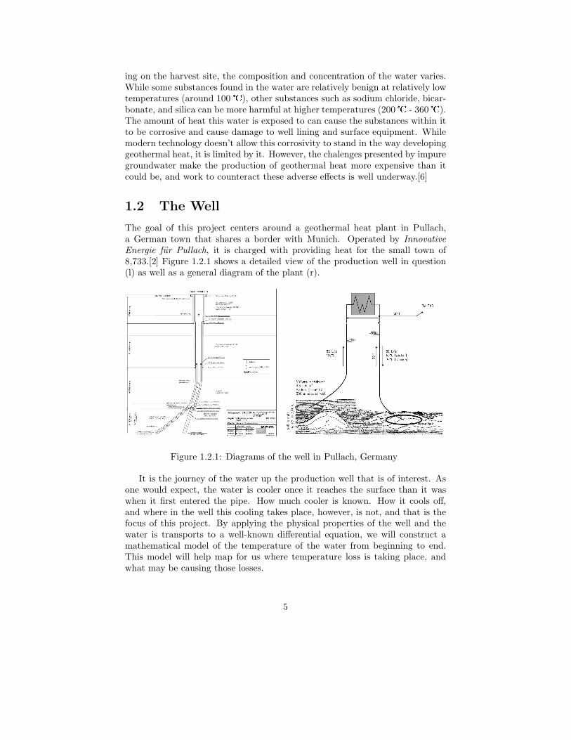
The goal of this project centers around a geothermal heat plant in Pullach,a German town that shares a border with Munich. Operated by InnovativeEnergie fur Pullach, it is charged with providing heat for the small town of8,733.[2] Figure 1.2.1 shows a detailed view of the production well in question(l) as well as a general diagram of the plant (r).

Figure 1.2.1: Diagrams of the well in Pullach, Germany

It is the journey of the water up the production well that is of interest. Asone would expect, the water is cooler once it reaches the surface than it waswhen it first entered the pipe. How much cooler is known. How it cools off,and where in the well this cooling takes place, however, is not, and that is thefocus of this project. By applying the physical properties of the well and thewater is transports to a well-known differential equation, we will construct amathematical model of the temperature of the water from beginning to end.This model will help map for us where temperature loss is taking place, andwhat may be causing those losses.

5

1.3 Derivation of the Heat Equation

On a fundamental level, this project is primarily concerned with heat transferin a vertical pipe. To begin construction of our desired model, we must firstderive a differential equation for heat transfer. In the simplest sense, we treatthe fluid in the pipe as a one dimensional rod of uniform width and length L.Figure 1.3.1 gives a graphic representation of the rod.

Figure 1.3.1: Diagram of 1-dimensional rod with heat flowing through a slice ofwidth ∆x.

1.3.1 Considering Conduction Through a Slice of a 1-D

Rod

We will examine heat flow through the small slice of the rod illustrated above.Table 1.3.1 describes physical properties of the pipe and rod as well as therepresentative variables of those properties.

Property Representative variableHeat flux through the point x at time t φ(x, t)Cross-sectional area of the pipe and slice ATemperature at point x at time t u(x, t)Specific heat at x c(x)Density at x ρ(x)

Table 1.3.1: Physical properties of the pipe

Typically, specific heat and density are considered to be uniform (constant)throughout the pipe, but in general they can vary according to position.

To quantify the heat energy flowing through the designated slice of the, weexamine the pipe’s physical properties, and derive energy from what we know.

6

To that end, heat energy (designated “H.E.”), is given by

H.E. = ρ(x)c(x)u(x, t)A∆x. (1.3.1)

If we examine the units on the right-hand side of (1.3.1), we see that

energy =mass

volume× energy

mass× degrees× degrees× volume

which verifies the equation given for H.E. We then apply the fundamental prin-ciple of conservation of energy (in this case, heat energy), to analyze further theenergy flow through the slice. The principle states that any change in temper-ature over time is due to heat flow across boundaries (in this case, x = x0 andx = x0 +∆x) and any heat generated within the rod. The latter quantity canbe expressed in terms of a new variable, Q(x, t), which gives the rate of heatenergy generated per unit of volume. In terms of units, Q is given by

Q(x, t) =energy

volume× time.

For this slice, the principle of conservation of heat energy can be mathematicallyexpressed as

∂H.E.

∂t≈ A [φ(x, t) − φ(x +∆x, t)] +Q(x, t)A∆x. (1.3.2)

Since we have an explicit definition of H.E., however, the left-hand side of(1.3.2) can be written as

∂H.E.

∂t= ρ(x)c(x)A∆x

∂u

∂t(1.3.3)

since x is fixed and ρ and c do not depend on t.The equation in (1.3.2) is given only as an approximation since some quanti-

ties are assumed to be constant and/or fixed in our slice. We can refine (1.3.2),however, if we consider the case where ∆x becomes infinitely small. To avoid atrivial 0 = 0, we first divide (1.3.2) by ∆x (after substituting in (1.3.3)) beforeapplying our limit. This gives us

ρ(x)c(x)∂u

∂t= lim

∆x→0

φ(x, t) − φ(x +∆x, t)

∆x+Q(x, t) (1.3.4)

or, equivalently,

ρ(x)c(x)∂u

∂t= −∂φ

∂x+Q(x, t). (1.3.5)

Note the use of equality and the fact that A was canceled out. Equation (1.3.5)can be alternatively derived over a larger region of the rod using more generalboundaries x = a and x = b and the fundamental theorem of calculus over theflux between a and b.

We now turn our attention to Fourier’s law of conductivity to complete ourderivation of the heat equation. The following properties of heat flow in generalserve as a premise to the law:

7

1. No energy flows if temperature in a medium is constant.

2. If temperature is not constant or uniform, heat energy flows from warmerregions to cooler regions.

3. Heat energy flow rate is directly proportional to temperature difference.

4. Different materials generate varying rates of heat energy flow (even iftemperature differences are consistent between the materials).

Mathematician Joseph Fourier experimented with these properties and came upwith the formula

φ(x, t) = −K0

∂u

∂x(1.3.6)

known as Fourier’s law of conductivity.[3] The constant K0 illustrates property4 and is known as the thermal conductivity constant of the material in question.The minus sign in (1.3.6) illustrates property 2 since an increase in temperatureto the right (i.e. as x increases) results in great heat energy flow to the left (i.e.as x decreases).

If we substitute the definition heat flux given in (1.3.6) into the principle ofconservation of heat energy given in (1.3.5), we arrive at the partial differentialequation

ρ(x)c(x)∂u

∂t= − ∂

∂x

(

−K0

∂u

∂x

)

+Q(x, t). (1.3.7)

In this model, we are assuming that the material in the rod is uniform, so ρ(x),c(x) and K0 may all be assumed to be constant. Therefore, (1.3.7) can berewritten as

ρc∂u

∂t= K0

∂2u

∂x2+Q(x, t). (1.3.8)

If there are no sources of heat external to our slice (i.e. Q ≡ 0), then we candivide by the constant ρc to gives us

∂u

∂t= κ

∂2u

∂x2(1.3.9)

where

κ =K0

ρc.

Equation (1.3.9) is known as the heat equation.

1.3.2 Looking at Multiple Dimensions

The heat equation given by (1.3.9) works if the medium being considered is one-dimensional and uniform. In general, however, we wish to examine heat flowthrough material that is multidimensional. In those cases, u is a multivariablefunction of each dimension as well as time, and a single partial derivative won’tdo. Additionally, the quantity φ given for flux becomes a vector, and is thereforewritten as φ.

8

To rework the heat equation to reflect these changes, we must look back tothe principle of heat energy conservation, expressed mathematically by (1.3.5).The 1-D partial derivative on the right-hand side is inadequate for φ, since wemust give partial derivatives for all dimensions. Since the number of dimensionsis generally arbitrary, we use the gradient operator ∇ and rewrite (1.3.5) as

ρc∂u

∂t= ∇ · φ+Q (1.3.10)

where (·) is the dot product operator. Note that we are going to assume earlythat our material is uniform and thus ρ and c are constant. With no extrasources of heat (as before), we also have Q = 0.

In multiple dimensions we also must take a second look at Fourier’s law ofconductivity. With u being multidimensional, the single partial derivative seenin (1.3.6) is again inadequate. We replace it with the gradient operator ∇ andget

φ = −K0∇u (1.3.11)

which verifies our earlier assertion that φ is vector-valued. Note that K0 isagain constant.

Subsituting (1.3.11) into (1.3.10) gives

ρc∂u

∂t= K0∇ · (∇u). (1.3.12)

By dividing by ρc and substituting κ as before, we are then left with

∂u

∂t= κ∇2u (1.3.13)

as our multidimensional equation, where ∇2 is the Laplacian operator.1

1.3.3 Examining Convection

When the material being considered is stationary, then the heat equation givenby (1.3.13) is satisfactory. When the material is more fluid and is itself flowing,however, we must examine how heat flows through the material in motion, aprocess known as convection. Suppose, then, that the fluid is moving withaverage velocity V (not necessarily constant). Then the flux vector for thematerial changes to reflect this new property and takes on a term to accountfor the motion of the material affecting the flow of heat energy. Fourier’s law ofconductivity is then rewritten as

φ = −K0∇u + ρcuV . (1.3.14)

As usual, we substitute (1.3.14) into the equation for conservation of heatenergy to arrive at our desired heat equation. Assuming again that Q = 0 and

1The Laplacian can alternatively be designated by a ∆ operator.

9

the material is uniform (i.e., ρ, c, and K0 are constant), we get

ρc∂u

∂t= −∇ · φ = −∇ · (−K0∇u+ ρcuV )

⇒ ρc∂u

∂t= ∇ · (K0∇u)−∇ · (ρcuV )

⇒ ρc∂u

∂t= K0∇2u− ρc∇ · (uV )

⇒ ∂u

∂t= κ∇2u− V · ∇u− u∇ · V

⇒ ∂u

∂t+ V · ∇u = κ∇2u− u∇ · V

where κ = K0

ρc, as before. In many cases, the velocity of the fluid is constant,

and so∇ · V = 0.

This gives us a heat equation that accounts for convection of

∂u

∂t+ V · ∇u = κ∇2u. (1.3.15)

1.4 Sturm-Liouville Theory

As we delve further into our problem with the heat equation, we will encountera special class of differential equations (in particular, boundary-value prob-lems) known as Sturm-Liouville problems (named for mathematicians Charles-Francois Sturm and Joseph Liouville) which have a special set of properties andidentities.

1.4.1 Definitions and Lagrange’s Identity

In general, Sturm-Liouville problems have the following form:

[p(x)y′]′ − q(x)y + λr(x)y = 0 (1.4.1)

a1y(0) + a2y′(0) = 0 (1.4.2)

b1y(1) + b2y′(1) = 0 (1.4.3)

where 0 < x < 1. It is generally assumed that p, p′, q, and r are all continuouson 0 ≤ x ≤ 1, and that p(x) > 0 and r(x) > 0 on the same interval. Analternate way of expressing (1.4.1) is by introducing the linear operator L[y] as

L[y] = − [p(x)y′]′

+ q(x)y (1.4.4)

and then rewrite the differential equation as

L[y] = λr(x)y. (1.4.5)

10

The linear operator defined by (1.4.4) is useful in a number of ways. If weassume the functions u(x) and v(x) satisfy the boundary-value problem definedby (1.4.1), then the operator allows us to compute

∫ 1

0

L[u]vdx =

∫ 1

0

− (pu′)′

v + quv dx. (1.4.6)

Integration by parts of the first term on the right-hand side gives us

∫ 1

0

− (pu′)′

v + quv dx = −pu′v∣

∣

∣

1

0

−∫ 1

0

pu′v′ + quv dx (1.4.7)

= −pu′v∣

∣

∣

1

0

−[

puv′∣

∣

∣

1

0

−∫ 1

0

(pv′)′

u+ quv dx

]

(1.4.8)

= −p (u′v − uv′)∣

∣

∣

1

0

+

∫ 1

0

L[v]u dx. (1.4.9)

If we rearrange the terms in the equality of the left-hand side of (1.4.6) and(1.4.9), then we can produce the equation

∫ 1

0

L[u(x)]v(x) − L[v(x)]u(x) dx = −p(x) [u(x)′v(x) − u(x)v′(x)]∣

∣

∣

1

0

(1.4.10)

which is known as Lagrange’s identity. Furthermore, if we also assume that u(x)and v(x) also satisfy the boundary conditions given by (1.4.2)-(1.4.3), then itcan be shown that (1.4.10) becomes

∫ 1

0

L[u(x)]v(x) − L[v(x)]u(x) dx = 0 (1.4.11)

provided a2 6= 0 and b2 6= 0. It is useful, now, if we define an inner product fortwo functions that satisfy a Sturm-Liouville problem. To that end, using ourfamiliar u and v, we define the following:

(u, v) =

∫ 1

0

u(x)v(x) dx (1.4.12)

which allows us to rewrite (1.4.11) as

(L[u], v)− (u, L[v]) = 0. (1.4.13)

Note that the inner product (1.4.12) is valid if both u and v are real-valuedfunctions. If they are complex functions, then the inner product takes the form

(u, v) =

∫ 1

0

u(x)v(x) dx (1.4.14)

where v(x) is the complex-conjugate of v(x). Note that even if u and v arereal-valued, then (1.4.14) remains valid since v(x) = v(x) for real v.

11

1.4.2 Eigenvalues and Eigenfunctions

In (1.4.1), the constant λ represents an eigenvalue of the differential equation.We now investigate several properties of a Sturm-Liouville problem’s eigenvaluesby way of a few theorems.

Theorem 1.4.1. All eigenvalues of the Sturm-Liouville problem given by (1.4.1)-(1.4.3) are real.

Proof. Suppose λ is a nonzero eigenvalue corresponding to a nonzero eigenfunc-tion φ(x). For this proof, we will allow for the possibility that λ and φ mayboth be complex. To the end, we define the two as follows:

λ := µ+ iν and φ(x) := U(x) + iV (x) (1.4.15)

where µ, ν, U , and V are all real. In the identity (1.4.13), allow both u = φand v = φ. This gives us

(L[φ], φ)− (φ, L[φ]) = 0 ⇒ (L[φ], φ) = (φ, L[φ]).

Using the identities given in (1.4.4) and (1.4.12), we have

(L[φ], φ) = (φ, L[φ]) ⇒ (λrφ, φ) = (φ, λrφ)

⇒∫ 1

0

λrφφ dx =

∫ 1

0

φλrφ dx.

Since r(x) is a real-valued function, we have r = r. From there, we have

λ

∫ 1

0

rφφ dx− λ

∫ 1

0

rφφ dx =(

λ− λ)

∫ 1

0

rφφ dx = 0.

Using the definition of φ given in (1.4.15), we find that

φφ = |φ|2 = U(x)2 + V (x)2

and so(

λ− λ)

∫ 1

0

r(x)[

U(x)2 + V (x)2]

dx = 0. (1.4.16)

Since r(x) and φ(x) are both nonzero, then the integrand in (1.4.16) cannot bezero. We are therefore left with

λ− λ = 0 ⇒ 2iν = 0 ⇒ ν = 0.

Therefore, λ must be real.

As a result of this theorem, solving Sturm-Liouville problems is made simplerbecause we are spared the task of seeking complex eigenvalues. It can also beshown that the eigenfunctions of Sturm-Liouville problems are also strictly real-valued.

This next theorem establishes the principle of orthogonality for the eigen-functions of Sturm-Liouville problems.

12

Theorem 1.4.2. If φ1(x) and φ2(x) are two eigenfunctions of the Sturm-Liouville problem given by (1.4.1)-(1.4.3) that correspond to distinct eigenvaluesλ1 and λ2, repsectively, then

∫ 1

0

r(x)φ1(x)φ2(x) dx = 0.

Proof. From (1.4.4), we know that

L[φ1] = λ1rφ1 and L[φ2] = λ2rφ2. (1.4.17)

Referring back to (1.4.12), if we allow u = φ1 and v = φ2, we have

(L[φ1], φ2)− (φ1, L[φ2]) = 0 ⇒ (λ1rφ1, φ2)− (φ1, λ2rφ2) = 0

⇒ λ1

∫ 1

0

r(x)φ1(x)φ2(x) dx − λ2

∫ 1

0

φ1(x)r(x)φ2(x) dx = 0

⇒ (λ1 − λ2)

∫ 1

0

r(x)φ1(x)φ2(x) dx = 0.

Since λ1 and λ2 are distinct, then λ1 − λ2 6= 0, and so

∫ 1

0

r(x)φ1(x)φ2(x) dx = 0.

The preceding theorem depended on the two eigenvalues being distinct withrespect to the two different eigenfunctions. In the following lemma, we will es-tablish that each eigenvalue of a Sturm-Liouville problem corresponds uniquelyto a certain eigenfunction.

Lemma. The eigenvalues of the Sturm-Liouville problem given by (1.4.1)-(1.4.3)are simple; or, each eigenvalue corresponds to one linearly independent eigen-function.

Proof. Suppose λ is an eigenvalue corresponding to two different linearly inde-pendent eigenfunctions φ1 and φ2. If we compute the Wronskian of φ1 and φ2,we have

W (φ1, φ2)(x) =

∣

∣

∣

∣

φ1(x) φ2(x)φ′1(x) φ′2(x)

∣

∣

∣

∣

= φ1(x)φ′

2(x)− φ′1(x)φ2(x) (1.4.18)

By definition, φ1 and φ2 are linearly independent if and only if the WronskianW (φ1, φ2)(x) is never 0. At the point x = 0, however, we have the following:

W (φ1, φ2)(0) = φ1(0)φ′

2(0)− φ′1(0)φ2(0)

= φ1(0)

(

−a1a2φ2(0)

)

−(

−a1a2φ1(0)

)

φ2(0)

= −a1a2φ1(0)φ2(0) +

a1a2φ1(0)φ2(0)

= 0

13

using both (1.4.2) and the assumption that a2 6= 0. Since the Wronskian is 0at some point, then φ1 and φ2 are not linearly independent, and we arrive ata contradiction to the premise at the beginning of the proof. Therefore, theeigenvalues of a Sturm-Liouville problem are simple.

1.4.3 Singular Sturm-Liouville Problems

With the Sturm-Liouville problems we have worked with so far, we have alwaysassumed regularity. In other words, we have always assumed that the propertiesassociated with p, q, etc. have all held true throughout the problem. But insome physical phenomena, one or more of these properties doesn’t hold, andtypically this occurs on a boundary (i.e. at x = 0 or x = 1). For the differentialequations that are almost of the Sturm-Liouville variety, we classify them assingular Sturm-Liouville problems. These kinds of problems have all the sameproperties as regular Sturm-Liouville problems on the open interval 0 < x < 1,but at least one property fails at either one or both boundaries. Singular Sturm-Liouville problems can also refer to differential equations defined on an openinterval (e.g. 0 < x <∞).

Consider the following differential equation

xy′′ + y′ + λxy = 0 or − (xy′)′

= λxy (1.4.19)

with boundary conditions

y(0) = 0 (1.4.20)

y(1) = 1 (1.4.21)

defined on the interval 0 < x < 1 with λ > 0. Notice that the criteria for beinga Sturm-Liouville problem appear to all be met, except for one. The coefficientr(x) = x must be positive over the closed interval (i.e. 0 ≤ x ≤ 1, yet w haver(0) = 0. Therefore, we can classify this bounday-value problem as a singularSturm-Liouville problem. To solve this problem, we can begin to proceed as wewould for any other problem, but we will have to deal with the singularity atx = 0 eventually. For now, though, we apply elementary methods.

Making the substitution t =√λx, we have y′(x) =

√λy′(t) and y′′(x) =

λy′′(t) by the chain rule. Making those substitutions into (1.4.19) gives us

tλ√λy′′ +

√λy′ + t

λ√λy = 0

which simplifies toty′′ + y′ + ty = 0. (1.4.22)

The differential equation (1.4.22) is easily identifiable as Bessel’s equation oforder 0. The solution in t is given by

y(t) = c1J0(t) + c2Y0(t)

14

with a general solution in x of

y(x) = c1J0

(√λx

)

+ c2Y0

(√λx

)

. (1.4.23)

where c1 and c2 are arbitrary constants and J0 and Y0 represent zero-order Besselfunctions of the first and second time, respectively. The explicit definitions forJ0 and Y0 are very intricate, and are therefore omitted. Turning our attentionnow to the boundary conditions given by (1.4.20)-(1.4.21), we see that J0(0) = 1,yet Y0(x) → −∞ as x→ 0. Because of this, we must choose c1 = 0 and c2 = 0(the trivial solution) so that (1.4.23) can satisfy the boundary conditions.

Obviously, the trivial solution isn’t satisfactory, so we need to find a workaroundso that y(x) can be non-trivial. One common method is to change one or bothboundary conditions to one that is less restrictive. In this case, we will mod-ify (1.4.20), since that is the one which was problematic before. Rather thanrequire y(0) = 0, we will instead require that y and y′ be bounded as x→ 0.

Since both Y0 and Y ′

0 are unbounded as x → 0, then we set c2 = 0. Thisleaves us with

y(x) = c1J0

(√λx

)

. (1.4.24)

Our second boundary condition, given by (1.4.21), gives us

y(1) = c1J0

(√λ)

= 0

which can be shown to have an infinite series of positive roots 0 < λ1 < λ2 <λ3 < · · · , giving us a set of eigenvalues. The corresponding eigenfunctions aregiven by

φn(x) = J0

(

√

λnx)

.

The constants c will be computed in the next section.This example is intended to illustrate how to take a singular Sturm-Liouville

problem can be solved by relaxing certain boundary conditions to the pointwhere intuitive eigenvalues and eigenfunctions can be computed. The use ofthis process, however, leaves open two important questions concerning singularSturm-Liouville problems:

1. What kind of boundary conditions can be allowed in a singular Sturm-Liouville problem?

2. How closely do the properties of the eigenvalues and eigenfunctions of asingular Sturm-Liouville problem mirror those of a regular Sturm-Liouvilleproblem? For example, are the eigenvalues real and are the eigenfunctionsorthogonal?

The answers to these questions depend on the identity

∫ 1

0

L[u]v − L[v]u dx = 0

and under what conditions it holds true for singular Sturm-Liouville problems.[1]

15

1.4.4 Method of Eigenfunction Expansion

In the example in the previous section, we outlined how to solve a singularSturm-Liouville problem, but we didn’t quite finish, since we left the constantsc arbitrary. To compute them numerically, we use a method known as eigen-function expansion.[3]

We begin by recalling Theorem 1.4.2, which said that the eigenfunctions ofa Sturm-Liouville problem are orthogonal. While this problem was singular,it can be shown that this orthogonality extends to Bessel functions as well.Therefore, our eigenfunctions given by (1.4.24) have the property

∫ 1

0

r(x)φm(x)φn(x) dx =

∫ 1

0

xφm(x)φn(x) dx = 0

when m 6= n. Using the superposition principle, we have that

y(x) =

∞∑

n=1

cnφn(x) =

∞∑

n=1

cnJ0

(

√

λnx)

. (1.4.25)

Multiplying both sides of (1.4.25) by xJ0(√λmx

)

and integrating with respectto x from 0 to 1 gives

∫ 1

0

xy(x)J0

(

√

λmx)

dx =

∞∑

n=1

cn

∫ 1

0

xJ0

(

√

λmx)

J0

(

√

λnx)

dx

which, because of orthogonality, quickly reduces to

∫ 1

0

xy(x)J0

(

√

λmx)

dx = cm

∫ 1

0

xJ2

0

(

√

λmx)

dx.

Therefore, we have

cm =

∫ 1

0xy(x)J0

(√λmx

)

dx∫ 1

0xJ2

0

(√λmx

)

dx. (1.4.26)

16

Chapter 2

Boundary Value Problem

Derivation and Solution

2.1 Problem Development

In this model, we examine the temperature of the fluid in a single stage ofthe pipe, where the pipe’s width is uniform throughout the section. We willsolve the steady-state of the problem (i.e. assume ∂T/∂t = 0) and assumethe liquid has Hagen-Poiseuille flow. Additionally, while we consider that thegeothermal properties of the soil surrounding the pipe has an effect on theliquid’s temperature profile, we will assume that the converse does not apply.To this end, we assume that the temperature profile of the liquid along the edgeof the pipe matches that of the surrounding soil. This model will be constructedin a Cartesian coordinate system with axes defined by the centerline of the pipeand its base (x = 0 and z = 0, respectively). We will assume symmetry aboutthe x-axis.

The pipe under consideration has the following physical properties:

Property Representative variable Typical numerical valueWidth R∗ 5 cmLength L∗ 1 km

Flow velocity W ∗ 32 L/s (.032 m/s)

Table 2.1.1: Physical properties of the pipe

To construct the model, we begin with the equation for heat energy of fluidflow in vector form:

ρcp

(

∂T

∂t+ u · ∇T

)

= k∇2T (2.1.1)

whereu = ux+ wz (2.1.2)

17

with x and z being unit vectors. The following table describes other variablesand coefficients in (2.1.1) as well as other variables and coefficients to be intro-duced in this section:

Variable Descriptionρ Density of the fluid in the pipecp The fluid’s specific heat capacityk The fluid’s conductivity constanth Heat transfer coefficientTg Thermal profile of the soil around the pipeκ The fluid’s thermal diffusivity

Table 2.1.2: Variables and coefficients in (2.1.1), etc.

This equation represents the conservation of energy of the fluid in the pipe.The definition in (2.1.2) allows us to expand the gradient in (2.1.1). With

this, and applying the steady-state assumption, (2.1.1) becomes

ρcp

(

∂T

∂t+ uTx + wTz

)

= k∇2T. (2.1.3)

Because we have assumed that the temperature profile of the liquid has nomeasurable effect on the soil around the pipe when in fact the converse is true,we have a Robin boundary condition of

kTx = −h (T − Tg) . (2.1.4)

Within h, we assume that the liquid’s flow is turbulent, and that there is aDittus-Boelter correlation with a Reynolds number Re = 105 and a relativelysmall Prandtl number (for water, this number is 7) which makes h large.

2.1.1 Nondimensionalization

Before proceeding further, we can nondimensionalize a number of variables forwith the substitutions

x⇒ R

z ⇒ L

w ⇒W

u⇒ R

LW

t⇒ L

W

Θ ⇒ 1

TAMB

(T − TAMB)

18

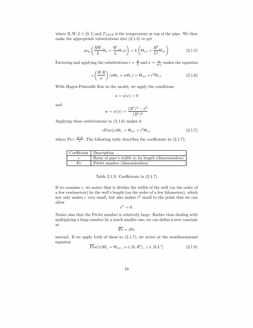
where R,W,L ∈ [0, 1] and TAMB is the temperature at top of the pipe. We thenmake the appropriate substitutions into (2.1.3) to get

ρcp

(

RW

LΘx +

W

LΘzw

)

= k

(

Θxx +R2

L2Θzz

)

(2.1.5)

Factoring and applying the substitutions ǫ = RLand κ = k

ρcpmakes the equation

ǫ

(

WR

κ

)

(uΘx + wΘz) = Θxx + ǫ2Θzz (2.1.6)

With Hagen-Poiseuille flow in the model, we apply the conditions

u = u(x) = 0

and

w = w(x) =(R∗)2 − x2

(R∗)4

Applying these substitutions to (2.1.6) makes it

ǫPew(x)Θz = Θxx + ǫ2Θzz (2.1.7)

where Pe= WRκ

. The following table describes the coefficients in (2.1.7):

Coefficient Descriptionǫ Ratio of pipe’s width to its length (dimensionless)Pe Peclet number (dimensionless)

Table 2.1.3: Coefficients in (2.1.7)

If we examine ǫ, we notice that it divides the width of the well (on the order ofa few centimeters) by the well’s length (on the order of a few kilometers), whichnot only makes ǫ very small, but also makes ǫ2 small to the point that we canallow

ǫ2 → 0.

Notice also that the Peclet number is relatively large. Rather than dealing withmultiplying a large number by a much smaller one, we can define a new constantas

Pe = ǫPe

instead. If we apply both of these to (2.1.7), we arrive at the nondimensionalequation

Pew(x)Θz = Θxx, x ∈ [0, R∗], z ∈ [0.L∗] (2.1.8)

19

with boundary conditions

Θx(0, z) = 0 (2.1.9)

Θ(R∗, z) = Θg(z) (2.1.10)

Θ(x, 0) = Θg(0). (2.1.11)

This can be solved using separation of variables.

2.1.2 Separation of Variables

To begin solving the BVP (2.1.8)-(2.1.11) using separation of variables, we firstdefine Θ(x, z) as a product of two single-variable functions φ(x) and Z(z), i.e.

Θ(x, z) = φ(x)Z(z). (2.1.12)

From (2.1.12), we can see that

Θz = φ(x)Z ′(z) and Θxx = φ′′(x)Z(z).

This turns (2.1.8) into

Pew(x)φ(x)Z ′(z) = φ′′(x)Z(z). (2.1.13)

To separate the variables, we divide both sides of (2.1.13) by w(x)φZ so thateach side of the equation is expressed in terms of only one variable, giving us

PeZ ′(z)

Z(z)=

φ′′(x)

w(x)φ(x). (2.1.14)

We now note that since both sides of (2.1.14) are expressed in terms of differentvariables, then the equality allows us to define each side as the same constant.We therefore define

PeZ ′(z)

Z(z)=

φ′′(x)

w(x)φ(x)= −λ

which can be separated into the system

PeZ ′ + λZ = 0 (2.1.15)

φ′′ + λw(x)φ = 0 (2.1.16)

giving us an eigenvalue problem in x and an amplitude problem in z.Before we solve (2.1.16), we first scale x and introduce the variable

ξ =x

R∗

which has a range of [0, 1]. This turns w(x) into

w(ξ) =(R∗)2 − ξ2(R∗)2

(R∗)4

=1− ξ2

(R∗)2.

20

Additionally, the chain rule tells us that

φ′′(ξ) =d2φ

dξ2=d2φ

dx2

(

dx

dξ

)2

+dφ

dx

d2x

dξ2= φ′′(x)(R∗)2 ⇒ φ′′(x) =

φ′′(ξ)

(R∗)2

where we see that (R∗)2 is a common denominator that can be cancelled. There-fore, the eigenvalue problem we are faced with is

φ′′(ξ) + λ(

1− ξ2)

φ(ξ) = 0 (2.1.17)

with boundary conditions

φ′(0) = 0 (2.1.18)

φ(1) = 0. (2.1.19)

2.2 Finding the Basis Eigenfunctions

We are faced with the task of finding the eigenvalues and eigenfunctions of thefollowing BVP:

φ′′(ξ) + λ(

1− ξ2)

φ(ξ) = 0 (2.2.1)

φ′(0) = 0 (2.2.2)

φ(1) = 0. (2.2.3)

We can quickly recognize this problem as a Sturm-Liouville problem, and so wecan derive the eigenfunctions from an orthogonal basis function ψ that solves

ψ′′(ξ) + µψ(ξ) = 0 (2.2.4)

ψ′(0) = 0 (2.2.5)

ψ(1) = 0 (2.2.6)

2.2.1 Finding the Basis Functions φ

The boundary value problem given by (2.2.4)-(2.2.6) has a general solution of

ψ(ξ) = c1 cos(√µξ) + c2 sin(

√µξ) (2.2.7)

where c1 and c2 are aribitrary constants. To apply (2.2.5), we first compute

ψ′(ξ) = −√µc1 sin(

√µξ) +

õc2 cos(

√µξ)

and then findψ′(0) =

√µc2 = 0 ⇒ c2 = 0 (2.2.8)

because we assume µ > 0. Applying (2.2.6) gives

ψ(1) = c1 cos(√µ) = 0. (2.2.9)

21

To avoid a trivial solution (i.e. c1 = 0), we consider cos(õ) = 0, which gives

us eigenvalues of

µi =π2

4(2i− 1)

2(2.2.10)

where i ∈ Z. Thus, our basis function is given by

ψi(ξ) = cos(√µiξ). (2.2.11)

To compute φ(ξ) from the basis ψ(ξ), we apply the superposition principleto give us

φ(ξ) =

∞∑

i=1

ciψi(ξ). (2.2.12)

2.2.2 Using Eigenfunction Expansion to Find Eigenvec-

tors

To compute the constants ci, we multiply both sides of (2.2.12) by ψj(ξ) andintegrate from 0 to 1 with respect to ξ. This gives us

∫ 1

0

φ(ξ)ψj(ξ)dξ =

∞∑

i=1

ci

∫ 1

0

ψi(ξ)ψj(ξ)dξ. (2.2.13)

Because of the orthogonality relation of the cosine function with itself, we canreduce the right-hand side of (2.2.13) and rewrite it as

∫ 1

0

φ(ξ)ψj(ξ)dξ = cj

∫ 1

0

ψ2

j (ξ)dξ (2.2.14)

which gives us the following formula for ci:

ci =

∫ 1

0φ(ξ)ψi(ξ)dξ∫ 1

0ψ2i (ξ)dξ

. (2.2.15)

With (2.2.15), we can proceed with finding the eigenvalue λ from (2.2.1).

2.2.3 Numerically Computing the Eigenvectors

Multiplying (2.2.15) by ψj(ξ) and then integrating from 0 to 1 with respect toξ gives us the following integral equation:

∫ 1

0

ψj(ξ)φ′′(ξ)dξ +

∫ 1

0

λ(

1− ξ2)

φ(ξ)ψj(ξ) = 0. (2.2.16)

From (2.2.12), we can rewrite the second term of (2.2.16) as

∞∑

i=1

ci

∫ 1

0

λ(

1− ξ2)

ψi(ξ)ψj(ξ)dξ. (2.2.17)

22

The first term, on the other hand, can be rewritten using integration by parts:

∫ 1

0

ψj(ξ)φ′′(ξ)dξ = ψj(ξ)φ

′(ξ)∣

∣

∣

1

0

−∫ 1

0

ψ′

j(ξ)φ′(ξ)dξ

= −[

ψ′

j(ξ)φ(ξ)∣

∣

∣

1

0

−∫ 1

0

ψ′′

j (ξ)φ(ξ)dξ

]

=

∫ 1

0

ψ′′

j (ξ)φ(ξ)dξ.

Using (2.2.4) and (2.2.15), the last integral can be rewritten as

∫ 1

0

ψ′′

j (ξ)φ(ξ)dξ = −µj

∫ 1

0

ψj(ξ)φ(ξ)dξ

= −µj

∫ 1

0

ψ2

j (ξ)dξ

= −1

2µjcj (2.2.18)

Now, with (2.2.17) and (2.2.18), we see that (2.2.16) is equivalent to

−1

2µjcj +

∞∑

i=1

ci

∫ 1

0

λ(

1− ξ2)

ψi(ξ)ψj(ξ)dξ = 0 (2.2.19)

which establishes a relation between the eigenvalues λ and the coefficients c.For computational purposes, we can restrict our sum in (2.2.19) to the first Nterms. Doing so allows us to write (2.2.19) as an algebraic equation with theform

1

2Mc = λBc (2.2.20)

where M is a diagonal matrix of the eigenvalues µ1, µ2, . . . µN , c is a columnvector of the coefficients c1, c2, . . . cN , and B is a matrix with

∫ 1

0

(

1− ξ2)

cos(√µiξ) cos(

√µjξ)dξ (2.2.21)

as its ij-th element.

2.3 Solving for the Nondimensional Θ

Now that we have computed our eigenfunctions φi(ξ), we can turn our attentionback to the nondimensional bounday-value problem in Θ(ξ, z) given in part by

Pe(1− ξ2)Θz = Θξξ (2.3.1)

Θ(ξ, 0) = Θg(0) (2.3.2)

23

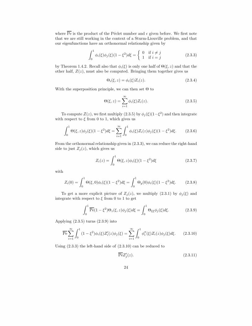
where Pe is the product of the Peclet number and ǫ given before. We first notethat we are still working in the context of a Sturm-Liouville problem, and thatour eigenfunctions have an orthonormal relationship given by

∫ 1

0

φi(ξ)φj(ξ)(1 − ξ2)dξ =

{

0 if i 6= j1 if i = j

(2.3.3)

by Theorem 1.4.2. Recall also that φi(ξ) is only one half of Θ(ξ, z) and that theother half, Z(z), must also be computed. Bringing them together gives us

Θi(ξ, z) = φi(ξ)Zi(z). (2.3.4)

With the superposition principle, we can then set Θ to

Θ(ξ, z) =

∞∑

i=1

φi(ξ)Zi(z). (2.3.5)

To compute Z(z), we first multiply (2.3.5) by φj(ξ)(1−ξ2) and then integratewith respect to ξ from 0 to 1, which gives us

∫ 1

0

Θ(ξ, z)φj(ξ)(1 − ξ2)dξ =

∞∑

i=1

∫ 1

0

φi(ξ)Zi(z)φj(ξ)(1 − ξ2)dξ. (2.3.6)

From the orthonormal relationship given in (2.3.3), we can reduce the right-handside to just Zj(z), which gives us

Zi(z) =

∫ 1

0

Θ(ξ, z)φi(ξ)(1 − ξ2)dξ (2.3.7)

with

Zi(0) =

∫ 1

0

Θ(ξ, 0)φi(ξ)(1 − ξ2)dξ =

∫ 1

0

Θg(0)φi(ξ)(1 − ξ2)dξ. (2.3.8)

To get a more explicit picture of Zj(z), we multiply (2.3.1) by φj(ξ) andintegrate with respect to ξ from 0 to 1 to get

∫ 1

0

Pe(1− ξ2)Θz(ξ, z)φj(ξ)dξ =

∫ 1

0

Θξξφj(ξ)dξ. (2.3.9)

Applying (2.3.5) turns (2.3.9) into

Pe

∞∑

i=1

∫ 1

0

(1− ξ2)φi(ξ)Z′

i(z)φj(ξ) =

∞∑

i=1

∫ 1

0

φ′′i (ξ)Zi(z)φj(ξ)dξ. (2.3.10)

Using (2.3.3) the left-hand side of (2.3.10) can be reduced to

PeZ ′

j(z). (2.3.11)

24

For the right-hand side, however, we must recall the boundary-value problemgoverning φ. Using that, we can rewrite the right-hand side as

−∞∑

i=1

λi

∫ 1

0

(1− ξ2)φi(ξ)Zi(z)φj(ξ)dξ (2.3.12)

where λi is the eigenvalue corresponding to the ith eigenfunction. Applying(2.3.3) gives us

−λjZj(z). (2.3.13)

Bringing (2.3.11) and (2.3.13), we can now rewrite (2.3.10) as

PeZ ′

j(z) = −λjZj(z). (2.3.14)

This ordinary differential equation in Z can easily be solved and has a generalsolution of

Zj(z) = A exp

(

−λj

Pez

)

(2.3.15)

where A is an arbitrary constant. To compute A, we recall the initial conditiongiven by (2.3.2) and compute

Zj(0) = A exp(0) ⇒ A = Zj(0) (2.3.16)

where Zj(0) is given explicitly above. We now have an explicit definition forZi(z) and, consequently, Θ(ξ, z).

25

Chapter 3

Results

With the model constructed, various data were numerically computed and col-lected using Matlab. They gave insight into the temperature profile of the waterin the Pullach well as well as where heat loss takes place. For all computations,an external profile Tg = 1 was used, but this can be easily changed and analyzedaccordingly.

3.1 Temperature Rise in Each Mode

Each φi(ξ) represents a different mode, or section of the pipe. Each mode hasits own width, and therefore its own temperature profile. The Matlab scripteigens.m was used to numerically compute the temperature profile at variousmodes. Figure 3.1.1 shows the temperature profile of the first three modes.The values along the vertical axis show the temperature relative to the thermalprofile of the edge of the well. Mathematically speaking, the temperature of thewater in terms of the temperature along the edge of the well is given by

Ti(ξ) = (1 + φi(ξ))Tg.

From the figure, we see that the profile of the first mode (the one at thebottom of the well), is the most stable, which isn’t surprising since the temper-ature profile immediately below the well should match (or be reasonably closeto) that of the edge of the bottom of the well. From there, the profiles get a bitmore hectic. Moving away from the center of the pipe causes increased variationin the temperature of the water. Figure 3.1.2 shows the profiles of the fourthand fifth modes.

Consistent with the previous figure, the profiles get more hectic and varymore as you move further from the center of the pipe. This time, however,there appears to be some sort of consistency between the profiles. Indeed, aswe plot higher modes, the shapes of the plots continue to look more similar toeach other, although the numbers can vary quite a bit.

26

Figure 3.1.1: Temperature profiles of φ1(ξ), φ2(ξ), and φ3(ξ).

Figure 3.1.2: Temperature profiles of φ4(ξ) and φ5(ξ).

27

The Matlab function nondim.m computes values for the whole model, varyingon the number of modes, the Peclet number, etc. With a low number of modes,we see similar results as with eigens.m: start with some stability and thenquickly see less. But with high numbers of modes, the process of becomingmore “hectic” slows down some, while the numbers do increase. Figure 3.1.3illustrates this with a comparison of N = 10 (left) and N = 5 (right). Note thedifferences in the ranges of their vertical axes.

Figure 3.1.3: Full models for N = 10 (left) and N = 5 (right).

Notice also the shapes of the graphs as you move along the z-axis. Both areexponential, but the N = 10 model has a deeper slope to it, suggesting a higherdrop in temperature. In fact, as N increases, so does this “depth”.

3.2 Variation of the Peclet Number

Recall that the Peclet number is directly proportional to the radius of the well(or, the radius of the current mode of the well) and inversely proportional to thethermal diffusivity of the water travelling in it. While the thermal diffusivity ismore or less constant, the radius is something that can vary significantly. Thus,the Peclet number is itself a moving target. Exploring how the model changesbased on the Peclet number yields some interesting results. Figure 3.1.3 aboveshowed both N = 10 and N = 5 with a Peclet number of 1,000. Figure 3.2.1below shows N = 5 with Peclet numbers of 100 and 500.

What is immediately noticeable is the difference in shape. As z increases,the model loses heat rather quickly for Pe = 100, but this is not the case forneither Pe = 500 nor Pe = 1000. We see a similar result with the same Pecletnumbers when N = 10, as illustrated by Figure 3.2.2.

It is also noteworthy that, in all the models and cases presented, heat tendsto be highest when approaching ξ = 1, before tapering off to 0 (as prescribedby the boundary conditions).

28

Figure 3.2.1: Model for N = 5 with Pe = 100 (left) and Pe = 500 (right).

Figure 3.2.2: Model for N = 10 with Pe = 100 (left) and Pe = 500 (right).

29

Chapter 4

Conclusions

The data shown in the previous chapter is representative of all the data com-puted and collected throughout this project. Going back to the original problem,we now examine the physical applications of our results to the Pullach well.

4.1 Applying our Results

Clearly, heat is lost in the production well as the water makes its 5 km journey tothe Earth’s surface. After looking at the results, the decay of the heat appears tobe exponential in nature, and so it would be expected that a deeper well wouldproduce more lost heat. Consequently, the results could be similar if moremodes were added. While initial temperature may be higher, the resulting heatloss could be greater. However, more research is needed to investigate whetherthere is causality here.

One notable result is that the water appears to become more heated as itnears the edge of the well before tapering off to match the temeperature profileof the well’s immediate surroundings. This is most likely a result of Fourier’slaw of conductivity which says, in part, that heat flows from hot to cold, withthe center of the well being warmer than the earth around it. The buildup ofheat near the edge is likely a result of the larger amount of water being nearthe edge as opposed to near the center.

The Peclet number carries a lot of influence in this model. If we are tointerpret a relatively high Peclet number to indicate a relatively wide well, thenwe can conclude that a narrower well leads to more heat loss. This could againbe a result of Fourier’s law, as the heat energy doesn’t have as far to travelbefore reaching its cold sink as it would in a wider well.

4.2 Future Work

Clearly, there is more to be done in this field. As mentioned previously, it shouldbe looked into whether the number of modes in a well is a factor in how much

30

heat is lost. This could eventually lead to wells with uniform radius from topto bottom, or to wells more resembling cones in the future, or something inbetween. Also, more attention must be paid to the geothermal profile of theearth around the well, and how it and the water can influence each other (asopposed to just the earth influencing the water).

It could very well be that heat loss can be attributed to water seeping out ofthe well while it flows to the surface. Therefore, more research into the mate-rials going into the wells is neceassary. This research can investigate materials’porousness as well as their ability to seal heat within the well.

Finally, the Peclet number showed itself to be an important factor in thismodel. While the radius of the well is a significant part of it, the velocityof the water flow is also significant. Research could therefore be done as towhether artificially speeding up or slowing down water flow has any effect ontemperature and heat loss. In addition, due to the impure nature of the waterbeing extracted, more precise measurements of the water’s thermal diffusivitywould yeild more precise Peclet numbers and therefore better models.

31

Bibliography

[1] William E. Boyce and Richard C. DiPrima. Elementary Differential Equa-tions and Boundary Value Problems. John Wiley & Sons, Inc., seventhedition, 2001.

[2] Bayerisches Landesamt fur Statistik und Datenverarbeitung [BavarianState Office for Statistics and Data Processing]. Fortschreibung desbevolkerungsstandes, 2011.

[3] Richard Habermann. Elementary Applied Differential Equations, WithFourier Series and Boundary Value Problems. Prentice Hall, third edition,1998.

[4] Gerald Katz. Environmental control technology development for geothermalenergy. Journal (Water Pollution Control Federation), 53(10):pp. 1447–1451, 1981.

[5] Erika Laszlo. Geothermal energy: An old ally. Ambio, 10(5):pp. 248–249,1981.

[6] Phillip Wright. Geothermal energy: A sustainable resource of enormous po-tential. JOM Journal of the Minerals, Metals and Materials Society, 50:38–40, 1998. 10.1007/s11837-998-0305-7.

32

Appendix A

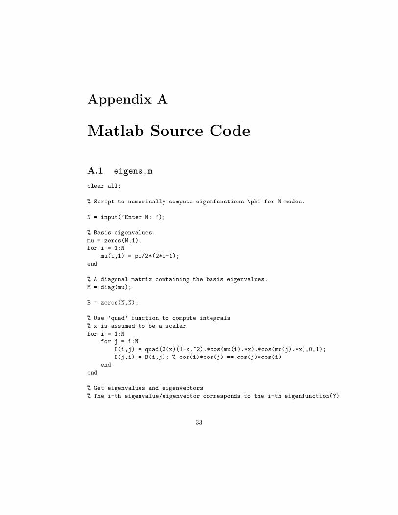
Matlab Source Code

A.1 eigens.m

clear all;

% Script to numerically compute eigenfunctions \phi for N modes.

N = input(’Enter N: ’);

% Basis eigenvalues.

mu = zeros(N,1);

for i = 1:N

mu(i,1) = pi/2*(2*i-1);

end

% A diagonal matrix containing the basis eigenvalues.

M = diag(mu);

B = zeros(N,N);

% Use ’quad’ function to compute integrals

% x is assumed to be a scalar

for i = 1:N

for j = i:N

B(i,j) = quad(@(x)(1-x.^2).*cos(mu(i).*x).*cos(mu(j).*x),0,1);

B(j,i) = B(i,j); % cos(i)*cos(j) == cos(j)*cos(i)

end

end

% Get eigenvalues and eigenvectors

% The i-th eigenvalue/eigenvector corresponds to the i-th eigenfunction(?)

33

[V,D] = eig(0.5*M,B);

% lambda is a column vector made out of the main diagonal of D (which

% contains the needed eigenvalues)

[lambda,ind] = sort(diag(D));

% Sort eigenvectors to correspond with their eigenvalues properly and

% normalize them to create matrix of coefficients.

c = V(:,ind);

for i = 1:N

c(:,i) = c(:,i)/c(1,i);

end

% Eigenfunctions

phi = cell(N,1);

for i = 1:N

phi{i} = @(x)sum(cos(mu.*x).*c(:,i));

end

% Numerically compute eigenfunctions

dx = 1/1000;

x = (0:dx:1)’; % length = 1/dx + 1

% The i-th column corresponds to the i-th eigenfunction

y = zeros(1/dx + 1,N);

for k = 1:N

for l = 1:(1/dx + 1)

y(l,k) = phi{k}(x(l));

end

end

A.2 nondim.m

function [T,x,z,lambda] = nondim(N,L,Pe,Tg)

% Function to numerically compute values for the full model over N modes.

% Sets default values for variables.

if nargin < 4

Tg = 1;

end

if nargin < 3

Pe = 1000;

end

34

if nargin < 2

L = 1;

end

if nargin == 0

N = 10;

end

% Basis eigenvalues.

mu = zeros(N,1);

for i = 1:N

mu(i,1) = pi/2*(2*i-1);

end

% A diagonal matrix containing the basis eigenvalues.

M = diag(mu);

B = zeros(N,N);

% Use ’quad’ function to compute integrals

% x is assumed to be a scalar

for i = 1:N

for j = i:N

B(i,j) = quad(@(x)(1-x.^2).*cos(mu(i).*x).*cos(mu(j).*x),0,1);

B(j,i) = B(i,j); % cos(i)*cos(j) == cos(j)*cos(i)

end

end

% Get eigenvalues and eigenvectors

% The i-th eigenvalue/eigenvector corresponds to the i-th eigenfunction

[V,D] = eig(0.5*M,B);

% lambda is a column vector made out of the main diagonal of D (which

% contains the eigenvalues for \phi)

[lambda,ind] = sort(diag(D));

% Sort eigenvectors to correspond with their eigenvalues properly and

% normalize them to create matrix of coefficients.

c = V(:,ind);

for i = 1:N

c(:,i) = c(:,i)/c(1,i);

end

% Eigenfunctions and amplitude functions.

phi = cell(N,1);

Z = cell(N,1);

35

for i = 1:N

phi{i} = @(x)sum(cos(mu.*x).*c(:,i));

Z{i} = @(z)exp(-lambda(i)./Pe.*z);

end

% Fourier coefficients

a = zeros(N,1);

for i = 1:N

a(i) = Tg.*quad(@(x)sumcosc(x).*(1-x.^2),0,1);

end

% Sub-function for computing coefficients

function y = sumcosc(x)

yy = 0;

for ii = 1:N

yy = yy + cos(mu(ii).*x).*c(ii,i);

end

y = yy;

end

% Numerically compute \Theta.

dx = 1/1000;

x = (0:dx:1)’; % Length = 1/dx + 1

dz = 1/1000;

z = (0:dz:L)’; % Length = L/dz + 1

Theta = zeros(1/dx + 1,L/dz + 1);

for k = 1:(L/dz + 1)

for l = 1:(1/dx + 1)

if mod(k,100) == 0 && l == 1

k

end

Theta(l,k) = theta(x(l),z(k));

end

end

% Subfunction for computing \Theta

function Thet = theta(x,z)

TThet = 0;

for ii = 1:N

TThet = TThet + a(ii)*phi{ii}(x)*Z{ii}(z);

end

Thet = TThet;

36

end

T = Theta;

end

37