Culture: An Empirical Investigation of Beliefs, Work, and Fertility

DISCUSSION PAPER SERIES

ABCD

www.cepr.org

Available online at: www.cepr.org/pubs/dps/DP5089.asp and www.ssrn.com/abstract=776764

www.ssrn.com/xxx/xxx/xxx

No. 5089

CULTURE: AN EMPIRICAL

INVESTIGATION OF BELIEFS, WORK AND FERTILITY

Raquel Fernández and Alessandra Fogli

INTERNATIONAL MACROECONOMICS, LABOUR ECONOMICS and

PUBLIC POLICY

ISSN 0265-8003

CULTURE: AN EMPIRICAL INVESTIGATION OF BELIEFS,

WORK AND FERTILITY

Raquel Fernández, New York University and CEPR Alessandra Fogli, New York University, Minneapolis Fed and CEPR

Discussion Paper No. 5089

May 2005

Centre for Economic Policy Research 90–98 Goswell Rd, London EC1V 7RR, UK

Tel: (44 20) 7878 2900, Fax: (44 20) 7878 2999 Email: [email protected], Website: www.cepr.org

This Discussion Paper is issued under the auspices of the Centre’s research programme in INTERNATIONAL MACROECONOMICS, LABOUR ECONOMICS and PUBLIC POLICY. Any opinions expressed here are those of the author(s) and not those of the Centre for Economic Policy Research. Research disseminated by CEPR may include views on policy, but the Centre itself takes no institutional policy positions.

The Centre for Economic Policy Research was established in 1983 as a private educational charity, to promote independent analysis and public discussion of open economies and the relations among them. It is pluralist and non-partisan, bringing economic research to bear on the analysis of medium- and long-run policy questions. Institutional (core) finance for the Centre has been provided through major grants from the Economic and Social Research Council, under which an ESRC Resource Centre operates within CEPR; the Esmée Fairbairn Charitable Trust; and the Bank of England. These organizations do not give prior review to the Centre’s publications, nor do they necessarily endorse the views expressed therein.

These Discussion Papers often represent preliminary or incomplete work, circulated to encourage discussion and comment. Citation and use of such a paper should take account of its provisional character.

Copyright: Raquel Fernández and Alessandra Fogli

CEPR Discussion Paper No. 5089

May 2005

ABSTRACT

Culture: An Empirical Investigation of Beliefs, Work and Fertility*

We study the effect of culture on important economic outcomes by using the 1970 Census to examine the work and fertility behaviour of women 30-40 years old, born in the US, but whose parents were born elsewhere. We use past female labour force participation and total fertility rates from the country of ancestry as our cultural proxies. These variables should capture, in addition to past economic and institutional conditions, the beliefs commonly held about the role of women in society, i.e. culture. Given the different time and place, only the beliefs embodied in the cultural proxies should be potentially relevant to women’s behaviour in the US in 1970. We show that these cultural proxies have positive and significant explanatory power for individual work and fertility outcomes, even after controlling for possible indirect effects of culture (e.g., education and spousal characteristics). We examine alternative hypotheses for these positive correlations and show that neither unobserved human capital nor networks are likely to be responsible. We also show that the effect of these cultural proxies is amplified the greater is the tendency for ethnic groups to cluster in the same neighbourhoods.

JEL Classification: J13, J21 and Z10 Keywords: cultural transmission, family, female labour force participation, fertility, immigrants, neighbourhoods and networks

Raquel Fernández Department of Economics New York University 269 Mercer St. New York, NY 10003 USA Tel: (1 212) 998 8908 Fax: (1 212) 995 4186 Email: [email protected] For further Discussion Papers by this author see: www.cepr.org/pubs/new-dps/dplist.asp?authorid=116433

Alessandra Fogli Department of Economics New York University 269 Mercer St. New York, NY 10003 USA Tel: (1 212) 998 0872 Email: [email protected] For further Discussion Papers by this author see: www.cepr.org/pubs/new-dps/dplist.asp?authorid=156704

*We thank Oriana Bandiera, Chris Flinn, David Levine, Fabrizio Perri, Jonathan Portes, Frank Vella, and seminar audiences at the SED, NBER, NYU, CERGE at Charles University, University of Cyprus, UC Berkeley, Stanford University, University of Iowa, Essex University, EUI, IGIER, and Pompeu Fabra University.

Submitted 13 May 2005

1. Introduction

As economists, we tend to study how individuals, with a given set of preferences and beliefs,

interact with economic incentives (provided mostly by markets), to produce outcomes. More

recently, we also emphasize the role of institutions, particularly in the longer run and at the

aggregate level.1 Thus, when we seek to explain variations in economic outcomes, we look pri-

marily at differences in components of individual or national budget sets (e.g., at variables such

as prices and incomes and at policies such as tax rates) and at differences in institutions (e.g.,

the extent of property protection or whether a political system is parliamentary or presidential).

This approach leaves out the possibility that preferences and beliefs, broadly speaking, themselves

have a systematic component that reflects past interactions of preferences, beliefs, markets, and

institutions. Variation in this systematic component—which we will call culture—therefore may

also be responsible for observed differences in outcomes.

With a few notable exceptions, the consequences of systematic differences in beliefs and

preferences have not been considered an appropriate topic for modern economic inquiry. In fact,

to attempt to explain differences in economic outcomes by appealing to differences in preferences

(and presumably beliefs) is often considered unscientific at best. As stated by Stigler and Becker

in their influential 1977 article "De Gustibus Non Est Disputandum:"

"We also claim, however, that no scientific behavior has been illuminated by as-

sumptions of differences in tastes. Instead, they along with assumptions of unstable

tastes, have been a convenient crutch to lean on when the analysis has bogged down.

They give the appearance of considered judgement, yet really have only been ad hoc

arguments that disguise analytical failures."

This approach, while sensible when variations in preferences and beliefs cannot be studied

in a rigorous fashion, is unnecessarily narrow if this variation is amenable to empirical analysis.2

1See Acemoglu, Johnson, and Robinson (2004) for the general thesis and a review of this literature. See alsoPersson and Tabellini (2003).

2 It is unclear whether Stigler and Becker regarded their criticism as also applying to differences in beliefs which,in a static framework, are indistinguishable from differences in preferences in their reduced form. Furthermore,to be fair, it is quite likely that the authors would agree that culture can and should be studied. They wouldinterpret culture, however, as arising from a deeper level of preferences (e.g., from a preference to be similar to one’sneighbors), or from costs in processing information that give rise to persistance in behavior even if the environmentchanges. This is, in fact, how the authors think of habits or customs. We have no quarrel with this interpretation,and in this sense we will not be trying to show that individuals differ in their "deeper" preferences, but rather intheir reduced-form appearance.

1

This paper seeks to address this deficiency by attempting to show that systematic variation in

preferences and beliefs (i.e, in culture) matters to important economic phenomena.

Culture is a rather hazy concept.3 Although developing a dynamic model of culture is beyond

the scope of this paper, it is useful to discuss some of the features of culture that are important

to our analysis. To be clear, we do not consider culture to be any more or less "primitive" than

markets or institutions. In our view, all three interact with one another over time and mutually

condition each other. Whether and how a market or institution operates, for example, may

depend on beliefs (e.g. on whether it is considered acceptable to buy and sell individuals as under

slavery, or whether women should count as full citizens and be allowed to vote in a "democracy")

and these beliefs themselves change in response to the experiences afforded by the economy and

the interests it creates.

Beliefs are a fundamental component of culture. These include not simply religious beliefs,

which are not for the most part empirically verifiable, but also beliefs that may be, in principle,

testable. Take, for example, the belief that children are better off if their mother stays home

to take care of them. This is a question about which, even today, people hold very different

beliefs. These beliefs are not based necessarily on scientific studies, but experimenting to obtain

more information is quite costly for any individual woman, and the counterfactual—how her child

will turn out otherwise—is difficult to establish. Beliefs and preferences are transmitted across

generations by the family and by local society (e.g., schools, religious organizations, neighborhood

composition, etc.). Thus, culture tends to evolve slowly over time in society, but can also suddenly

shift as new information (e.g., new anecdotes or changes in neighborhood composition or media

availability) becomes more widely diffused.4 We will not, in any case, attempt to provide a

more abstract and rigorous definition of culture here, but rather attempt to identify, in individual

behavior, something that we can think of as beliefs or norms that operate in a systematic fashion.5

We choose to investigate the effect of culture on important economic decisions by studying

women’s work and fertility decisions. The focus on women is not accidental. Fertility and

women’s participation in the formal labor market vary widely across time and space. The

hypothesis that a significant part of this variation can be explained by different beliefs as to

3As defined by the Merriam-Webster dictionary, culture is a) “the integrated pattern of human knowledge, belief,and behavior that depends upon man’s capacity for learning and transmitting knowledge to succeeding generations”;b) “the customary beliefs, social forms, and material traits of a racial, religious, or social group”.

4Empirically it is difficult to distinguish between beliefs, information, and preference transmission and we willnot attempt to do so.

5For a discussion of social norms (and some definitions) see, for example, Elster (1989).

2

the appropriate role of women in society, i.e. by culture, as opposed to solely economic and

institutional variation, seems particularly apt in this context and the economic importance of

these decisions is incontrovertible.6

A challenge in the analysis of culture is to separate its effects from those due to markets

and institutions. One way around this problem is to study outcomes for women born in one

country (the United States, in our case) but whose parents were born in another country. It

can be argued that these women share similar markets and formal institutions but have possibly

different cultural heritages as reflected in their parents’ country of origin. Furthermore, rather

than use a dummy variable for the woman’s country of ancestry as a proxy for culture (which does

not make explicit why it matters to be of Mexican ancestry, say, relative to Swedish), we take past

labor force participation and fertility variables from the country of ancestry as our cultural proxies.

These variables should reflect, in addition to whatever economic and institutional conditions were

prevalent in the country at that time, the cultural beliefs that then reigned as to the appropriate

role for women in society. While the economic and institutional conditions should no longer be

relevant for the second-generation American women (as neither the country nor the time period is

the same), the beliefs embodied in these variables may still matter if parents and/or neighborhood

transmitted them to the next generation.

We use the 1970 Census to study work and fertility outcomes for women and use 1950 values

of female labor force participation (LFP) and total fertility rates (TFR) in the country of ancestry

as the cultural proxies.7 We find that the cultural proxies are significant to both work and fertility

outcomes. In order to ensure that these results are not driven by parental characteristics that

differ in a systematic fashion by country of origin, we control as well for variables that themselves

are likely to be influenced by culture, such as a woman’s education, or the education and income

of her spouse.8 We also control for local geographic variation in markets and institutions by

including metropolitan standard area fixed effects and we cluster observations at the country-of-

ancestry level. In all cases, we find that culture, as reflected in our proxy variables of LFP or

TFR in 1950, is a quantitatively and statistically significant determinant of women’s work and

6Pencavel’s (1998) study of women’s market work and wages from the mid 1970s to the mid 1990s, for example,concludes that changes in wages can at most account for half of the observed change in work behavior across cohorts.Fernández, Fogli, and Olivetti (2004) present a model of endogenous preference evolution through family experienceand explore the role of these preferences in increasing female labor force participation. See Goldin (1990) for ahistory of women and work in the US.

7Later decades of the Census do not ask for the country of birth of a respondent’s parents and 1950 is as farback as one can go to obtain female LFP and TFR for a non-trivial number of countries.

8Our data set does not permit us to observe the financial and educational backgrounds of parents directly.

3

https://www.researchgate.net/publication/24091879_Mothers_and_Sons_Preference_Formation_and_Female_Labor_Force_Dynamics?el=1_x_8&enrichId=rgreq-de211374d6dfda50bcaa5a39b0707b21-XXX&enrichSource=Y292ZXJQYWdlOzUwMDk1Njc7QVM6MTA2NjIyNjE3NjUzMjUxQDE0MDI0MzIyMjE5MTc=

https://www.researchgate.net/publication/46553019_The_Market_Work_Behavior_and_Wages_of_Women_1975-94?el=1_x_8&enrichId=rgreq-de211374d6dfda50bcaa5a39b0707b21-XXX&enrichSource=Y292ZXJQYWdlOzUwMDk1Njc7QVM6MTA2NjIyNjE3NjUzMjUxQDE0MDI0MzIyMjE5MTc=

https://www.researchgate.net/publication/227466718_Understanding_the_Gender_Gap_An_Economic_History_of_American_Women?el=1_x_8&enrichId=rgreq-de211374d6dfda50bcaa5a39b0707b21-XXX&enrichSource=Y292ZXJQYWdlOzUwMDk1Njc7QVM6MTA2NjIyNjE3NjUzMjUxQDE0MDI0MzIyMjE5MTc=

fertility outcomes. A one standard deviation increase in LFP in 1950 is associated with about a

one week increase in weeks worked per year (or about a 7.5% increase in hours worked) in 1970;

a one standard deviation increase in TFR in 1950 is associated with approximately 0.4 extra

children, a 14% increase in the number of children in 1970.9

The major concern our analysis needs to address is whether there exists some omitted variable

that is driving our results and that is unrelated to culture but correlated with LFP and TFR in

1950 in the country of ancestry. The main suspects for this role are unobserved human capital

or the "quality" of the networks available to these women. Unobserved human capital may

be a culprit if differences in parental education levels lead to differences in unobserved human

capital in ways not captured by the formal education level of their children. Alternatively, if

the human capital of one’s ethnic group is an important input in the formation of own human

capital (as argued by Borjas (1992,1995)), or if it is an input in the ethnic network that helps

individuals find employment, then systematic differences across ethnic groups may be responsible

for our results. We address these concerns in a few ways. We use the General Social Survey

(GSS) to control directly for the parent’s level of education and show that our results are robust

to these additional controls. We also construct measures of ethnic human capital by using the

1940 Census to calculate the average education of immigrants by country of origin. This variable

should proxy both for parental human capital and for the human capital embodied in the ethnic

network available to the woman. We find that this variable is significant in explaining how much

women work (though not fertility) but the effect of the cultural proxy remains robust. We also

construct a similar measure of ethnic human capital for second-generation immigrants from the

same generation as our sample and obtain similar results.

Our most revealing test, however, is related to men. We show that our cultural proxies

are unable to explain men’s work behavior though they have explanatory power for the number

of children men have. This is reassuring since, if female LFP in 1950 were able to positively

and significantly explain the work behavior of the male counterparts of our women (i.e., men

born in the US whose parents were born in a foreign country), this would cast serious doubts as

to whether the cultural variable was primarily capturing attitudes towards women rather than

some unobserved economic difference by country of ancestry. The fertility variable, on the other

hand, is able to capture cultural preferences towards family size which may be shared by men and

9We also used country dummies in our analysis. We show that our cultural proxies are able to explain asignificant portion of the variation in the coefficients of the country dummies.

4

https://www.researchgate.net/publication/24091333_Ethnic_Capital_And_Intergenerational_Mobility?el=1_x_8&enrichId=rgreq-de211374d6dfda50bcaa5a39b0707b21-XXX&enrichSource=Y292ZXJQYWdlOzUwMDk1Njc7QVM6MTA2NjIyNjE3NjUzMjUxQDE0MDI0MzIyMjE5MTc=

women.

The investigation of culture and men rather naturally leads us to examine a related question:

Whose culture is important in deciding a married woman’s work and fertility—her own or her

husband’s? We show that the cultural proxies of both spouses play an important role, though

perhaps surprisingly the husband’s culture seems to be more important in driving his wife’s work

outcomes.10 We also investigate whether variation across country of ancestry in the average

proportion of individuals from the same ancestry in a neighborhood matters for cultural trans-

mission. In particular, is the impact of culture larger for those groups that tend to cluster in

the same neighborhoods? We find that the answer is yes, strengthening our prior that culture is

transmitted both by family and by local society (e.g. neighborhood, schools, church, etc.).

Our paper is organized as follows. The next section contains a brief review of the empirical

literature.11 Section 3 presents our empirical strategy and Section 4 our results. We examine

robustness to sample selection and estimation techniques in Section 5. Section 6 examines

competing explanations. Section 7 investigates whether it is a woman’s or her husband’s culture

that matters for her outcomes and section 8 studies the role of ethnic density in the neighborhood.

Section 9 concludes.

2. A Brief Literature Review

The idea that culture can influence economic outcomes is, of course, not a new one. Max

Weber’s celebrated thesis at the beginning of the 20th century argued that a specific culture—the

"Protestant ethic"—was conducive to capitalist accumulation.12 More recently, culture plays a

central role in Landes’ (1998) explanation for differences in economic growth across countries, and

Putnam (2000) stresses the role of trust, and more generally of "social capital", in facilitating

economic exchange and efficient governance.13

There is little quantitative evidence, however, that demonstrates that culture is a significant

determinant of important economic outcomes. Not surprisingly, the relatively small literature

in this field has often focused either on immigrants or on individuals from different ethnic back-

10This evidence is also in line with Fernández et al (2004). They show that a quantitatively important factorexplaining whether a man’s wife works is whether his own mother worked when he was growing up. This findingholds even after controlling for education, income, and other family background variables. Whether his motherworked or not is probably influenced by her beliefs about women’s role, which may then have been transmitted toher son and thus influenced any household bargaining/decision affecting his wife’s work outcome.11See Bisin and Verdier (2000) for a model of the family and endogenous cultural transmission and Cole, Mailath,

and Postlewaite (1992) for a model of endogenous social norms and how these affect savings and growth.12More recently, Barro and McCleary (2003) examine the effect of religion on economic growth.13See Weil’s (2004) very nice chapter that reviews the research on culture and growth.

5


https://www.researchgate.net/publication/220879623_Bowling_Alone_The_Collapse_and_Revival_of_American_Community?el=1_x_8&enrichId=rgreq-de211374d6dfda50bcaa5a39b0707b21-XXX&enrichSource=Y292ZXJQYWdlOzUwMDk1Njc7QVM6MTA2NjIyNjE3NjUzMjUxQDE0MDI0MzIyMjE5MTc=

grounds to investigate the effect of culture. Using ethnic dummy variables, Reimers (1985) is

an early attempt to examine the role of ethnicity in married women’s labor force participation

in the US. She finds mixed evidence in favor of ethnic background mattering, which perhaps is

not surprising given that ethnic groups vary substantially in the length of time they have been in

the US. Employing a similar strategy, but focusing solely on immigrants which allows them to

ensure a greater degree of homogeneity, Carroll, Rhee, and Rhee (1994) examine whether culture

can help explain different savings rates by comparing saving patterns of immigrants to Canada.

They find no evidence of cultural effects on savings. Their analysis, however, faces important

data limitations: they control only for broad regions of origin and they do not have data on

individual wealth.

Giuliano (2004) and Antecol (2000) both use quantitative home-country variables to study

the effect of culture. Giuliano attempts to show that Western European second-generation

immigrants to the US tend to replicate the family living arrangements of their country of origin.

Her main thesis is that the sexual revolution interacted with different family models in the early

1970s to increase the proportion of individuals who live at home in Southern European countries

but not in Northern ones, and that this differential pattern of behavior is reflected in the behavior

of second-generation individuals in the US. Giuliano shows that individuals of Southern Europe

ancestry tend to have a higher probability of living at home in the US.

Antecol (2000) studies the effect of male and female LFP in the country of ancestry on

the inter-ethnic gender gap in labor force participation rates in the US.14 For first generation

immigrants, labor force participation in the US increases for women and decreases for men as a

function of female LFP in the home country.15 For second-and-higher-generation immigrants,

the total effect of female LFP appears to be positive for both men and women. These results

are interesting, but why culture should produce this pattern is unclear and alternative hypotheses

(e.g., other country characteristics) are not examined. Furthermore, the focus on first-generation

immigrants leaves open the reasonable possibility that these results are the product of systematic

economic differences across countries of origin. The analysis of second-and-higher-generation

immigrants is also problematic since the data set does not permit one to identify the exact

generation and hence some families may have been in the country for many generations whereas

others may be second generation. Our analysis, by using the 1970 census and focusing exclusively

14Antecol (2001) conducts a similar study for the gender wage gap.15The results with respect to male LFP are not reported.

6

https://www.researchgate.net/publication/222829610_An_Examination_of_Cross-Country_Differences_in_the_Gender_Gap_in_Labor_Force_Participation_Rates?el=1_x_8&enrichId=rgreq-de211374d6dfda50bcaa5a39b0707b21-XXX&enrichSource=Y292ZXJQYWdlOzUwMDk1Njc7QVM6MTA2NjIyNjE3NjUzMjUxQDE0MDI0MzIyMjE5MTc=

on second-generation immigrants, avoids both sets of problems.

In addition to the above studies focussing on immigrants, there has also been work using

measures of attitudes towards women’s role within a country. Levine (1993), for example, finds

that attitudes, as reflected in responses to GSS questions, are an important predictor of whether

any particular woman works in a given year, but that the attitude variables are not able to explain

the increase in women’s labor force participation during the 70s and early 80s. Vella (1994) uses

Australian data and likewise finds that attitude variables are important determinants of the extent

of women’s involvement in market work.

There is also a small literature on cultural effects on fertility. Guinnane, Moehling, and

O Grada (2004) have a very interesting study on Irish fertility in the US in 1910. They find

that although Irish fertility fell in the US relative to couples in Ireland, Irish immigrants still

had larger families than the native-born population in the US (conditional on differences in other

observable population characteristics). This points to culture playing a role, both for first and

second generation Irish-Americans. Interestingly, they do not find that to be the case for second

generation German immigrants. Our analysis, which will be based on a much larger set of

countries, will allow us to study whether such a cultural effect exists more generally.

Blau (1992) examines whether (and why) the fertility behavior of first-generation immigrant

women differs from that of the native born in the US. This is a difficult question to analyze as

she must face issues such as who selects into immigration, and the possible disrupted and delayed

fertility behavior that may result from immigration. Interestingly, she finds that the home

country variable (TFR) enters positively and significantly into explaining the fertility behavior

of immigrant women in 1970 and 1980. By examining second-generation women in the US, our

analysis will allow us to focus on questions of cultural transmission with fewer concerns about

selection and disruption due to immigration.

3. The Empirical Strategy, Datasets, and Sample Selection

As discussed in the introduction, our empirical strategy is to isolate the effect of culture from

those of markets and institutions by studying the work and fertility outcomes of women who were

born in and reside in the US, but whose parents were born in another country. Our main data set

is the 1% 1970 Form 2 Metro Sample of the U.S. Census. We use the 1970 Census since this is the

7

https://www.researchgate.net/publication/5191583_The_Fertility_of_Immigrant_Women_Evidence_from_High_Fertility_Source_Countries?el=1_x_8&enrichId=rgreq-de211374d6dfda50bcaa5a39b0707b21-XXX&enrichSource=Y292ZXJQYWdlOzUwMDk1Njc7QVM6MTA2NjIyNjE3NjUzMjUxQDE0MDI0MzIyMjE5MTc=

https://www.researchgate.net/publication/222599720_The_Effect_of_Non-Traditional_Attitudes_on_Married_Women's_Labor_Supply?el=1_x_8&enrichId=rgreq-de211374d6dfda50bcaa5a39b0707b21-XXX&enrichSource=Y292ZXJQYWdlOzUwMDk1Njc7QVM6MTA2NjIyNjE3NjUzMjUxQDE0MDI0MzIyMjE5MTc=

last year in which individuals were explicitly asked where their parents were born.16 The 1970

Census does not provide the country of birth of an individual’s mother when both parents were

born outside U.S. Hence, we use the father’s birthplace to assign a country-of-ancestry culture

to the second-generation women in our sample.

Our main sample consists of married women who are 30-40 years old. Women in this

age range have completed their education but are still far from retirement considerations. We

exclude women living in farms or working in agricultural occupations, as well as those living in

group quarters (e.g. prisons, and other group living arrangements such as rooming houses and

military barracks).17 There are 87,305 women who are born in U.S. and satisfy these criteria.18

About 11% of them have fathers who were born outside U.S. and are thus included in our sample.

From this group we eliminate those who respond to the question about their father’s birthplace

with a continent or a geographical area from which a country cannot be identified.

To study women’s labor outcomes we mainly use either the number of weeks worked in

the previous year or the number of hours worked in the previous week. In the 1970 Census,

information on weeks and hours worked is reported in intervals.19 We compute our measure of

weeks and hours worked by assigning the midpoint of each interval. The Census also asks women

to record the number of children ever born to them. We use the response to this question to

study fertility.

For our cultural proxies we want to use variables that would capture the beliefs as to the

appropriate role of women and, relatedly, the ideal family size, for the woman’s country of ancestry.

Female labor force participation and the total fertility rate of women are a priori good candidates

for this. Ex ante, however, it is not clear for what year we should choose to measure female LFP

and TFR for the country of ancestry. As the women in our sample are 30-40 in 1970 and were

born in U.S., their parents must have been in the US by 1930-1940, depending on the precise age

16 In subsequent decades, individuals were asked to declare their "ancestry" and thus it is impossible to distinguishbetween individuals whose families have been in the US for many generations from those that are second-generationAmericans. Using earlier decades, on the other hand, runs into the problem that we cannot obtain female LFPand TFR for more than a handful of countries prior to 1950.17We exclude the following occupations (based on the 1950 Census definition): farmers (owners and tenants),

farm managers, farm foremen, farm laborers as wage workers, farm laborers as unpaid family workers, and farmservice laborers as self-employed.18We exclude from the sample women born in U.S. outlying areas and territories (American Samoa, Guam, Puerto

Rico, U.S. Virgin Islands, Other US Possessions). We also exclude from the sample women who were born in U.S.but in an unidentified state. Their inclusion does not alter the results.19The number of weeks worked in the previous year are recorded in 6 intervals: 1-13 weeks, 14-26, 27-39, 40-47,

48-49, 50-52. All other observations are coded as N/A and treated as zeros in this work. The number of hoursworked in the previous week are recorded in 8 intervals: 1-14 hours, 15-29, 30-34, 35-39, 40, 41-48, 49-59, 60+. Allother observations are coded as N/A and treated as zeros in this work.

8

of the woman. Thus, on the one hand, it could be argued that the values of the culture proxy

variables around 1930-40 or even a decade or two earlier would best reflect the culture of the

country of ancestry. On the other hand, one could argue that the values that parents and society

transmit are best reflected in what the counterparts of these women are doing in the country of

ancestry in 1970. Of course, in both cases the values of the variables reflects not only culture,

but the economics and institutions of the country over time. The point is, however, that neither

the economy nor the institutions should have particular relevance to explain the work and fertility

outcomes of the women in our sample as they were born and raised in the US. Data limitations, in

any case, do not permit us to use years prior to 1950 since values for neither variable are available

for more than a handful of countries prior to that year. Consequently, we choose female LFP

and TFR in 1950 in the country of ancestry as our benchmark cultural proxies but also explore

1960 and 1970 values as well.

The cross-country data for 1950 female LFP and TFR are from the International Labor

Organization (ILO) and the United Nation’s Demographic Yearbook, respectively. Female LFP

is the rate of economically active population for women over ten years of age.20 The TFR is the

average number of children a hypothetical cohort of women, from the ages of 15 to 49, would have

at the end of their reproductive period if they were subject during their whole lives to the fertility

rates of a given period and if they were not subject to mortality. It is expressed as number of

children per woman.

We conclude our selection by eliminating from our sample all women whose fathers were born

in countries that became centrally-planned economies around World War II.21 The rationale for

doing this is that the parents of our women must have been in the US by 1940. Hence, the

parents did not live through the profound transformations in the economies, institutions, and

cultures that these countries experienced over that period and using data from the 50s and later

would thus not capture the correct culture for these individuals. We also excluded Russia since

the revolution was in 1917 and the parents may or may not have been there for any substantial

length of time thereafter. For robustness, we have also run our regressions with Russia and our

results are unaffected. Lastly, solely in order to be able to make meaningful comparisons across

20The active population includes: persons in "paid" or "unpaid" employment, members of the armed forces(including temporary members) and the unemployed (including first-time job seekers). "Unpaid" employmentincludes: employers, own-account workers and members of producers’ cooperative; unpaid family workers, personsengaged in the production of economic goods and services for own and household consumption, and apprenticeswho receive pay.21We eliminated Albania, Bulgaria, Czechoslovakia, Hungary, Poland, Romania, Yugoslavia, Estonia, Latvia, and

Lithuania.

9

averages of women by country of ancestry, we also eliminated those countries with fewer than 15

observations.22 Since our regressions are all run at the individual level, including these small

number of observations does not affect our results. Our final sample consists of 6774 women and

25 countries of ancestry.

In Table I we report the summary statistics at the country level. Our countries are mainly

European (17 countries), with a few countries in the Americas (Canada, Cuba, and Mexico), some

in Asia (China, Japan, and the Philippines), and some in the Middle East (Syria and Lebanon).

Female LFP in 1950 is on average 24.4 with a standard deviation of 11.4. It varies dramatically by

country: from 7% in Lebanon to over 50% in Turkey. The TFR in 1950 also shows large variation:

from 6.9 children in Turkey and Mexico to 2.1 in Austria. The average across countries is 3.7

with a standard deviation of 1.8. Interestingly, the cross-country correlation of female LFP and

TFR in 1950 is practically zero (0.002).

The women in our sample are on average 35.7 years old, have 3.1 children and worked on

average 15.2 weeks in the previous year and 10.2 hours in the previous week. There is large

dispersion in the number of weeks and hours worked: the standard deviation of weeks worked is

20.9 and the standard deviation of hours worked is 16.3. The standard deviation in the number

of children is 1.8. Comparing the women in our sample with their counterparts whose fathers

were born in U.S., the latter have a similar number of children on average (3.0). Women with

fathers born in the US on average worked more: 18.2 weeks a year and 13.1 hours a week. The

standard deviation is also slightly higher: 21.8 and 18.0 for weeks and hours, respectively. The

summary statistics for the women in our sample are reported in Table A1 of the Appendix.

The differences across work and fertility in 1970 for the women in our sample can also be

seen when we group observations by country of ancestry, as done in Table 1. Women with Cuban

fathers worked 27.6 weeks (15.2 hours) on average, while women with Syrian fathers worked 9.5

weeks (5.1 hours) on average. Women with Mexican fathers on average have 4.2 kids whereas

women from Turkey have 2.2. The standard deviation in work and fertility by country of ancestry

(3.9 and 2.6 for weeks and hours worked, respectively, and 0.4 for children) is considerably smaller

than the standard deviation in these variables across all women. It is also smaller than the

standard deviation by country of ancestry in the levels of 1950 LFP and TFR.

Figure 1 plots the average number of hours worked in the previous week by the women in

our sample by country of ancestry against the logarithm of the female LFP in 1950 in the same

22 Iceland, Luxemburg, Korea, India, Iran, and Jordan.

10

country. Figure 2 plots the average number of children of the women in our sample by country

of father’s birthplace against the logarithm of the TFR in 1950 in that country. The correlation

between hours worked and female LFP is 0.25 (0.06 for weeks) whereas that between children and

TFR is 0.13. From the fertility graph, one can clearly see two groups of countries: one which has

undergone the fertility revolution and another which has yet to do so.

For our analysis to be meaningful, culture should evolve relatively slowly over the time period

in which we are interested. Otherwise, in general, the beliefs transmitted from parents to children

would not be captured by past values of female LFP and TFR. Although we cannot examine the

values for our cultural proxies twenty years earlier to verify this, we can look at them 20 years

later, i.e., in 1970. The rank (Spearman) correlation across countries for female LFP in 1950 and

1970 is 0.93; the rank correlation for those same two decades in TFR is 0.85. Figures 3 and 4

show the evolution of female LFP and TFR for each of our 25 countries (and the US as well) from

1950 to 2000. With the exception of Turkey, which shows a dramatic decrease in female LFP for

several decades, most countries show an increase in female LFP with little change in their relative

ranking. The Pearson and rank correlations for our set of 25 countries between 1950 and 2000

is 0.51 and 0.50, respectively. Over time, TFR has decreased in all countries. The Pearson and

rank correlations in TFR from 1950 to 1995 remain remarkably high: 0.86 and 0.70, respectively.

4. Results

We estimate the following model:

Zisj = β0 + β01Xi + β2 eZj + fs + εisj (4.1)

where Zisj is the work/fertility decision of woman i who resides in the Standard Metropolitan Sta-

tistical Area (SMSA) s and is of ancestry j.23 In Xi we include a set of individual characteristics

which varies with the specification considered, fs is a full set of dummies for the metropolitan area

of residence and eZj is the proxy for culture—our variable of interest—which is assigned by the coun-try of father’s birthplace. Since the key variable on the right-hand side only varies by country of

ancestry, all the standard errors we report are corrected for clustering at the country-of-ancestry

level.

Tables II and III present our main results. In the first column, the amount worked (either

23A SMSA is an area consisting of a large population center and adjacent communities (usually counties) thathave a high degree of economic and social interaction with that center. A total of 117 SMSAs (including not residingin an SMSA) are identified in the data.

11

weeks worked in the previous year or hours worked in the previous week, depending on the table)

by individual i is regressed on the cultural proxy for work–female LFP in 1950 assigned by country

of ancestry–and on a full set of dummies for the woman’s metropolitan area of residence.24 The

coefficient on the cultural variable is positive and strongly significant, indicating that women

whose parents were born in countries where women participated less in the work force tend to

work less themselves.

There may be many reasons for the positive partial correlation above that have little to do

with culture. In particular, women’s parents may differ in a systematic fashion by country of

origin, in a way that affects their daughter’s propensity to work. For example, if higher levels of

education increase the incentives to work, and if it is less costly for a woman to become educated

if her parents come from a high female LFP country (e.g., because these parents are themselves

more educated or because they have higher income or wealth), then this correlation would be

due to the correlation between parental characteristics by country of origin and female education.

This would suggest that, if information on parental characteristics is unavailable, we may want

to control directly for a woman’s level of education. By doing so, we are left however only with

the direct effect of culture on how much a woman works.

The regression results from including a series of female characteristics, in particular the

woman’s age, her age squared, and a set of dummy variables to capture her level of education

(below high school (omitted), high school degree (High School), some college, and at least a college

degree (College +)) are reported in the second column. As expected, more educated women tend

to work more. The direct effect of culture remains positive and statistically significant, albeit

somewhat smaller in magnitude indicating that a woman’s education and female LFP in her

country of ancestry tend to be positively correlated.

It may also be instructive to include the characteristics of a woman’s husband in our regression

analysis. In part, this may allow us to distinguish between the effect of a woman’s education and

that of her husband’s (or of her husband’s income) on her degree of participation in the formal

labor market. How a woman’s desire to work may itself affect her choice of husband is unclear.

On the one hand, if higher levels of male education tend to be associated with a more positive

attitude towards women working, then that may lead to a positive relationship between culture

and male education. On the other hand, if a woman plans to work, she may be less concerned

24We examine hours in addition to weeks as the former may be considered a better variable since it may correspondmore closely to the choices individuals make (how many hour to work rather than a number of weeks).

12

with her husband’s income level and more concerned with other idiosyncratic features.25

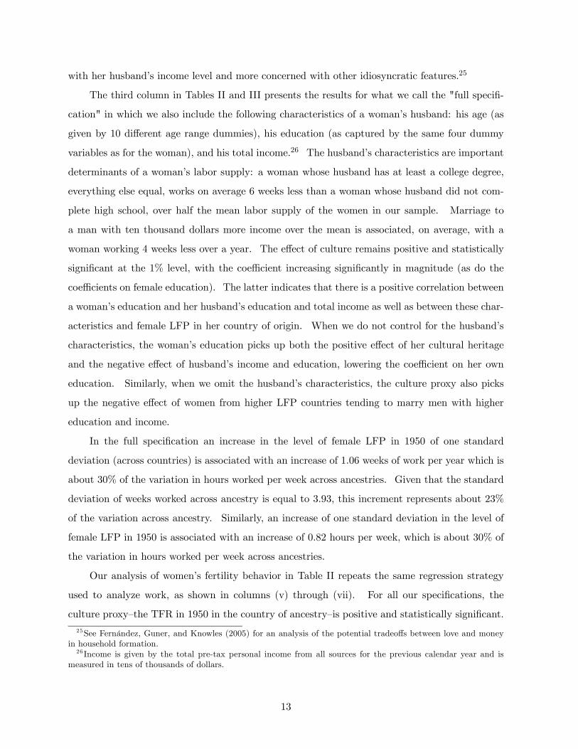
The third column in Tables II and III presents the results for what we call the "full specifi-

cation" in which we also include the following characteristics of a woman’s husband: his age (as

given by 10 different age range dummies), his education (as captured by the same four dummy

variables as for the woman), and his total income.26 The husband’s characteristics are important

determinants of a woman’s labor supply: a woman whose husband has at least a college degree,

everything else equal, works on average 6 weeks less than a woman whose husband did not com-

plete high school, over half the mean labor supply of the women in our sample. Marriage to

a man with ten thousand dollars more income over the mean is associated, on average, with a

woman working 4 weeks less over a year. The effect of culture remains positive and statistically

significant at the 1% level, with the coefficient increasing significantly in magnitude (as do the

coefficients on female education). The latter indicates that there is a positive correlation between

a woman’s education and her husband’s education and total income as well as between these char-

acteristics and female LFP in her country of origin. When we do not control for the husband’s

characteristics, the woman’s education picks up both the positive effect of her cultural heritage

and the negative effect of husband’s income and education, lowering the coefficient on her own

education. Similarly, when we omit the husband’s characteristics, the culture proxy also picks

up the negative effect of women from higher LFP countries tending to marry men with higher

education and income.

In the full specification an increase in the level of female LFP in 1950 of one standard

deviation (across countries) is associated with an increase of 1.06 weeks of work per year which is

about 30% of the variation in hours worked per week across ancestries. Given that the standard

deviation of weeks worked across ancestry is equal to 3.93, this increment represents about 23%

of the variation across ancestry. Similarly, an increase of one standard deviation in the level of

female LFP in 1950 is associated with an increase of 0.82 hours per week, which is about 30% of

the variation in hours worked per week across ancestries.

Our analysis of women’s fertility behavior in Table II repeats the same regression strategy

used to analyze work, as shown in columns (v) through (vii). For all our specifications, the

culture proxy—the TFR in 1950 in the country of ancestry—is positive and statistically significant.

25See Fernández, Guner, and Knowles (2005) for an analysis of the potential tradeoffs between love and moneyin household formation.26 Income is given by the total pre-tax personal income from all sources for the previous calendar year and is

measured in tens of thousands of dollars.

13

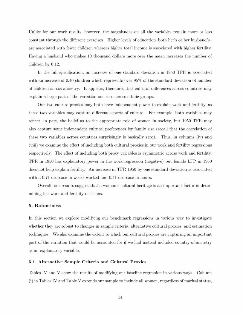
Unlike for our work results, however, the magnitudes on all the variables remain more or less

constant through the different exercises. Higher levels of education—both her’s or her husband’s—

are associated with fewer children whereas higher total income is associated with higher fertility.

Having a husband who makes 10 thousand dollars more over the mean increases the number of

children by 0.12.

In the full specification, an increase of one standard deviation in 1950 TFR is associated

with an increase of 0.40 children which represents over 95% of the standard deviation of number

of children across ancestry. It appears, therefore, that cultural differences across countries may

explain a large part of the variation one sees across ethnic groups.

Our two culture proxies may both have independent power to explain work and fertility, as

these two variables may capture different aspects of culture. For example, both variables may

reflect, in part, the belief as to the appropriate role of women in society, but 1950 TFR may

also capture some independent cultural preferences for family size (recall that the correlation of

these two variables across countries surprisingly is basically zero). Thus, in columns (iv) and

(viii) we examine the effect of including both cultural proxies in our work and fertility regressions

respectively. The effect of including both proxy variables is asymmetric across work and fertility.

TFR in 1950 has explanatory power in the work regression (negative) but female LFP in 1950

does not help explain fertility. An increase in TFR 1950 by one standard deviation is associated

with a 0.71 decrease in weeks worked and 0.41 decrease in hours.

Overall, our results suggest that a woman’s cultural heritage is an important factor in deter-

mining her work and fertility decisions.

5. Robustness

In this section we explore modifying our benchmark regressions in various way to investigate

whether they are robust to changes in sample criteria, alternative cultural proxies, and estimation

techniques. We also examine the extent to which our cultural proxies are capturing an important

part of the variation that would be accounted for if we had instead included country-of-ancestry

as an explanatory variable.

5.1. Alternative Sample Criteria and Cultural Proxies

Tables IV and V show the results of modifying our baseline regression in various ways. Column

(i) in Tables IV and Table V extends our sample to include all women, regardless of marital status,

14

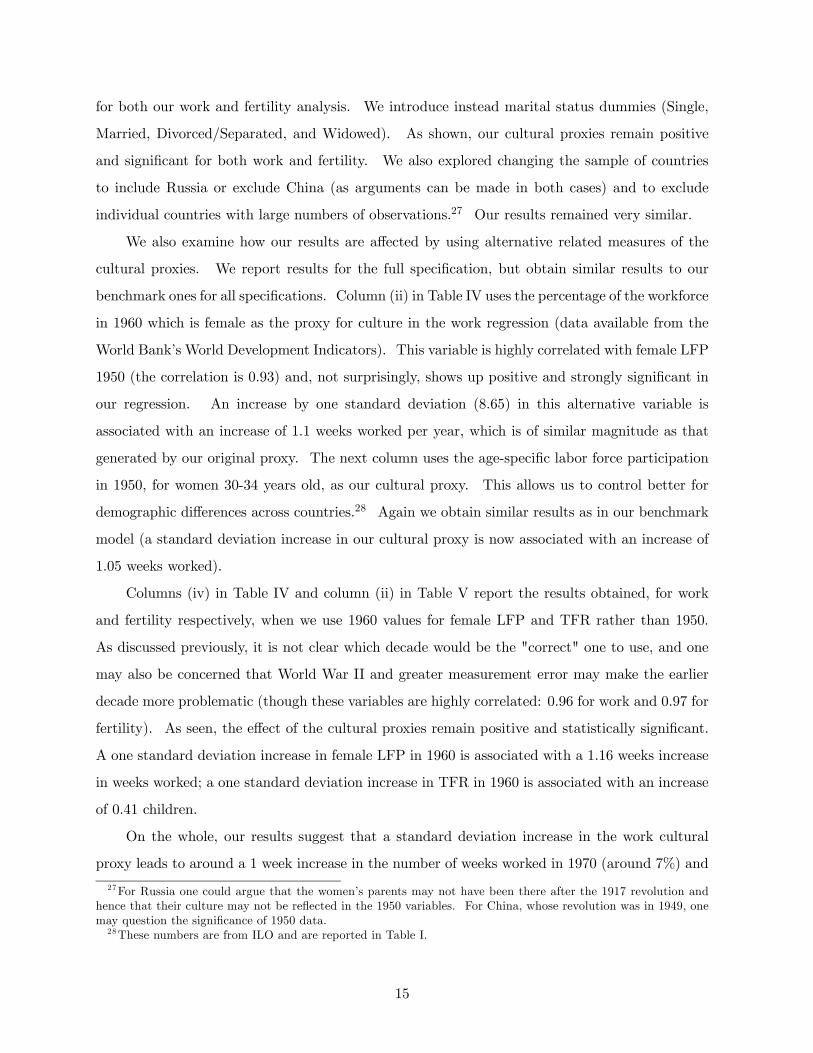
for both our work and fertility analysis. We introduce instead marital status dummies (Single,

Married, Divorced/Separated, and Widowed). As shown, our cultural proxies remain positive

and significant for both work and fertility. We also explored changing the sample of countries

to include Russia or exclude China (as arguments can be made in both cases) and to exclude

individual countries with large numbers of observations.27 Our results remained very similar.

We also examine how our results are affected by using alternative related measures of the

cultural proxies. We report results for the full specification, but obtain similar results to our

benchmark ones for all specifications. Column (ii) in Table IV uses the percentage of the workforce

in 1960 which is female as the proxy for culture in the work regression (data available from the

World Bank’s World Development Indicators). This variable is highly correlated with female LFP

1950 (the correlation is 0.93) and, not surprisingly, shows up positive and strongly significant in

our regression. An increase by one standard deviation (8.65) in this alternative variable is

associated with an increase of 1.1 weeks worked per year, which is of similar magnitude as that

generated by our original proxy. The next column uses the age-specific labor force participation

in 1950, for women 30-34 years old, as our cultural proxy. This allows us to control better for

demographic differences across countries.28 Again we obtain similar results as in our benchmark

model (a standard deviation increase in our cultural proxy is now associated with an increase of

1.05 weeks worked).

Columns (iv) in Table IV and column (ii) in Table V report the results obtained, for work

and fertility respectively, when we use 1960 values for female LFP and TFR rather than 1950.

As discussed previously, it is not clear which decade would be the "correct" one to use, and one

may also be concerned that World War II and greater measurement error may make the earlier

decade more problematic (though these variables are highly correlated: 0.96 for work and 0.97 for

fertility). As seen, the effect of the cultural proxies remain positive and statistically significant.

A one standard deviation increase in female LFP in 1960 is associated with a 1.16 weeks increase

in weeks worked; a one standard deviation increase in TFR in 1960 is associated with an increase

of 0.41 children.

On the whole, our results suggest that a standard deviation increase in the work cultural

proxy leads to around a 1 week increase in the number of weeks worked in 1970 (around 7%) and

27For Russia one could argue that the women’s parents may not have been there after the 1917 revolution andhence that their culture may not be reflected in the 1950 variables. For China, whose revolution was in 1949, onemay question the significance of 1950 data.28These numbers are from ILO and are reported in Table I.

15

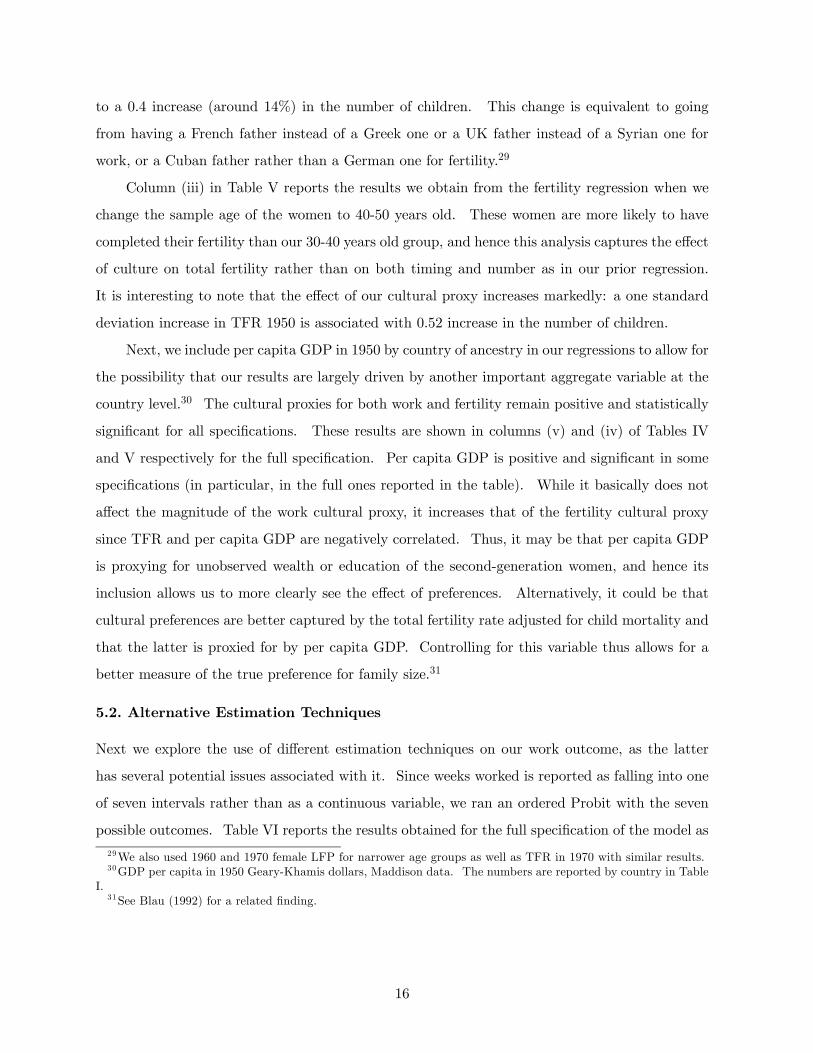
to a 0.4 increase (around 14%) in the number of children. This change is equivalent to going

from having a French father instead of a Greek one or a UK father instead of a Syrian one for

work, or a Cuban father rather than a German one for fertility.29

Column (iii) in Table V reports the results we obtain from the fertility regression when we

change the sample age of the women to 40-50 years old. These women are more likely to have

completed their fertility than our 30-40 years old group, and hence this analysis captures the effect

of culture on total fertility rather than on both timing and number as in our prior regression.

It is interesting to note that the effect of our cultural proxy increases markedly: a one standard

deviation increase in TFR 1950 is associated with 0.52 increase in the number of children.

Next, we include per capita GDP in 1950 by country of ancestry in our regressions to allow for

the possibility that our results are largely driven by another important aggregate variable at the

country level.30 The cultural proxies for both work and fertility remain positive and statistically

significant for all specifications. These results are shown in columns (v) and (iv) of Tables IV

and V respectively for the full specification. Per capita GDP is positive and significant in some

specifications (in particular, in the full ones reported in the table). While it basically does not

affect the magnitude of the work cultural proxy, it increases that of the fertility cultural proxy

since TFR and per capita GDP are negatively correlated. Thus, it may be that per capita GDP

is proxying for unobserved wealth or education of the second-generation women, and hence its

inclusion allows us to more clearly see the effect of preferences. Alternatively, it could be that

cultural preferences are better captured by the total fertility rate adjusted for child mortality and

that the latter is proxied for by per capita GDP. Controlling for this variable thus allows for a

better measure of the true preference for family size.31

5.2. Alternative Estimation Techniques

Next we explore the use of different estimation techniques on our work outcome, as the latter

has several potential issues associated with it. Since weeks worked is reported as falling into one

of seven intervals rather than as a continuous variable, we ran an ordered Probit with the seven

possible outcomes. Table VI reports the results obtained for the full specification of the model as

29We also used 1960 and 1970 female LFP for narrower age groups as well as TFR in 1970 with similar results.30GDP per capita in 1950 Geary-Khamis dollars, Maddison data. The numbers are reported by country in Table

I.31See Blau (1992) for a related finding.

16

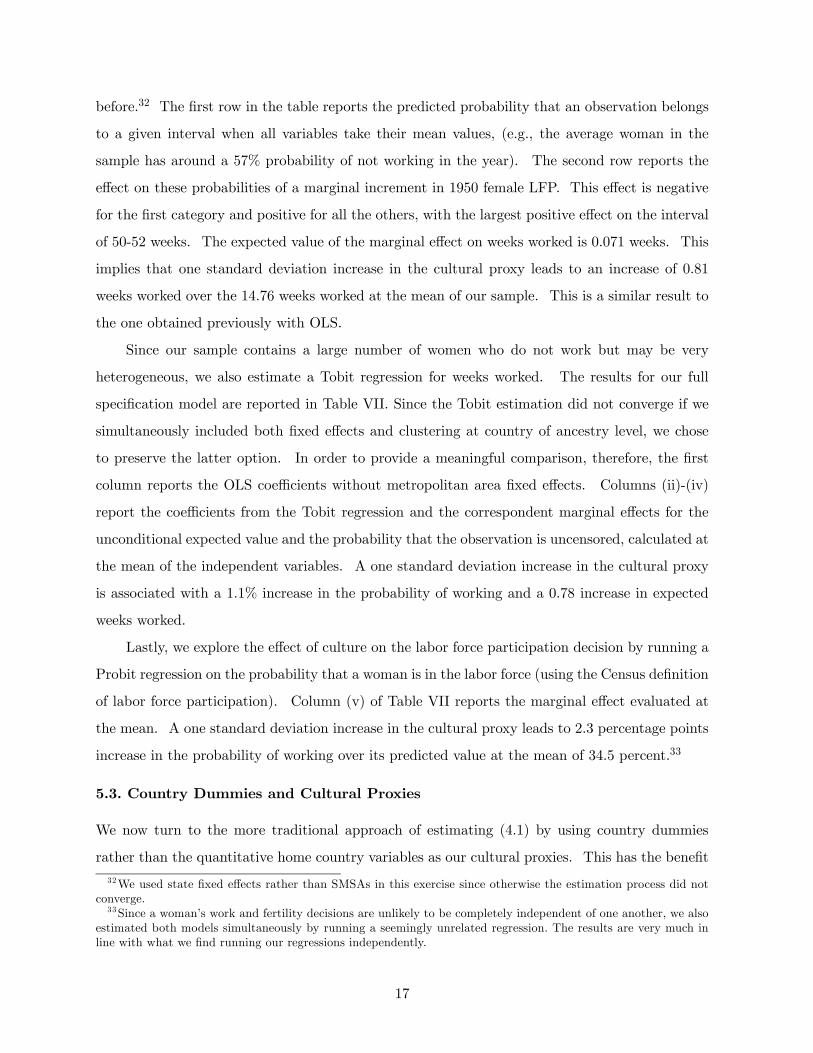
before.32 The first row in the table reports the predicted probability that an observation belongs

to a given interval when all variables take their mean values, (e.g., the average woman in the

sample has around a 57% probability of not working in the year). The second row reports the

effect on these probabilities of a marginal increment in 1950 female LFP. This effect is negative

for the first category and positive for all the others, with the largest positive effect on the interval

of 50-52 weeks. The expected value of the marginal effect on weeks worked is 0.071 weeks. This

implies that one standard deviation increase in the cultural proxy leads to an increase of 0.81

weeks worked over the 14.76 weeks worked at the mean of our sample. This is a similar result to

the one obtained previously with OLS.

Since our sample contains a large number of women who do not work but may be very

heterogeneous, we also estimate a Tobit regression for weeks worked. The results for our full

specification model are reported in Table VII. Since the Tobit estimation did not converge if we

simultaneously included both fixed effects and clustering at country of ancestry level, we chose

to preserve the latter option. In order to provide a meaningful comparison, therefore, the first

column reports the OLS coefficients without metropolitan area fixed effects. Columns (ii)-(iv)

report the coefficients from the Tobit regression and the correspondent marginal effects for the

unconditional expected value and the probability that the observation is uncensored, calculated at

the mean of the independent variables. A one standard deviation increase in the cultural proxy

is associated with a 1.1% increase in the probability of working and a 0.78 increase in expected

weeks worked.

Lastly, we explore the effect of culture on the labor force participation decision by running a

Probit regression on the probability that a woman is in the labor force (using the Census definition

of labor force participation). Column (v) of Table VII reports the marginal effect evaluated at

the mean. A one standard deviation increase in the cultural proxy leads to 2.3 percentage points

increase in the probability of working over its predicted value at the mean of 34.5 percent.33

5.3. Country Dummies and Cultural Proxies

We now turn to the more traditional approach of estimating (4.1) by using country dummies

rather than the quantitative home country variables as our cultural proxies. This has the benefit

32We used state fixed effects rather than SMSAs in this exercise since otherwise the estimation process did notconverge.33Since a woman’s work and fertility decisions are unlikely to be completely independent of one another, we also

estimated both models simultaneously by running a seemingly unrelated regression. The results are very much inline with what we find running our regressions independently.

17

of not requiring the relation between culture and outcomes to be linear in the cultural proxy.

Furthermore, it may allow different features of culture to play a role in work and fertility outcomes

other than those captured in LFP and TFR 1950. It has the previously discussed drawback,

however, of not specifying how culture matters.

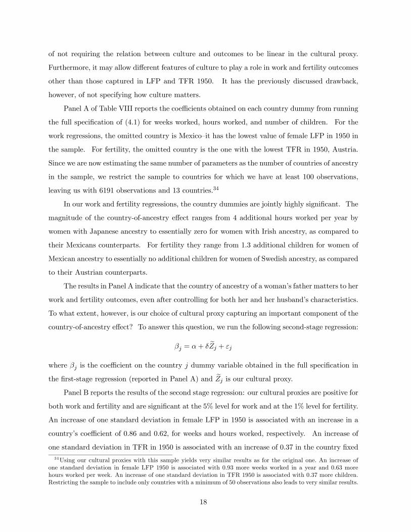
Panel A of Table VIII reports the coefficients obtained on each country dummy from running

the full specification of (4.1) for weeks worked, hours worked, and number of children. For the

work regressions, the omitted country is Mexico—it has the lowest value of female LFP in 1950 in

the sample. For fertility, the omitted country is the one with the lowest TFR in 1950, Austria.

Since we are now estimating the same number of parameters as the number of countries of ancestry

in the sample, we restrict the sample to countries for which we have at least 100 observations,

leaving us with 6191 observations and 13 countries.34

In our work and fertility regressions, the country dummies are jointly highly significant. The

magnitude of the country-of-ancestry effect ranges from 4 additional hours worked per year by

women with Japanese ancestry to essentially zero for women with Irish ancestry, as compared to

their Mexicans counterparts. For fertility they range from 1.3 additional children for women of

Mexican ancestry to essentially no additional children for women of Swedish ancestry, as compared

to their Austrian counterparts.

The results in Panel A indicate that the country of ancestry of a woman’s father matters to her

work and fertility outcomes, even after controlling for both her and her husband’s characteristics.

To what extent, however, is our choice of cultural proxy capturing an important component of the

country-of-ancestry effect? To answer this question, we run the following second-stage regression:

βj = α+ δ eZj + εj

where βj is the coefficient on the country j dummy variable obtained in the full specification in

the first-stage regression (reported in Panel A) and eZj is our cultural proxy.Panel B reports the results of the second stage regression: our cultural proxies are positive for

both work and fertility and are significant at the 5% level for work and at the 1% level for fertility.

An increase of one standard deviation in female LFP in 1950 is associated with an increase in a

country’s coefficient of 0.86 and 0.62, for weeks and hours worked, respectively. An increase of

one standard deviation in TFR in 1950 is associated with an increase of 0.37 in the country fixed34Using our cultural proxies with this sample yields very similar results as for the original one. An increase of

one standard deviation in female LFP 1950 is associated with 0.93 more weeks worked in a year and 0.63 morehours worked per week. An increase of one standard deviation in TFR 1950 is associated with 0.37 more children.Restricting the sample to include only countries with a minimum of 50 observations also leads to very similar results.

18

effect. Furthermore, the adjusted R squares are sizeable, especially for fertility, indicating that

variation in female LFP and in TFR in 1950 explains an important part of the differences in the

country coefficients.35 Hence, using these variables rather than the more "black-box" approach

of a country dummy, appears to be a good strategy.

6. Competing Explanations

The prior section established that our results are robust to a number of alternative variable

definitions, sample selection criteria, and estimation techniques. The main remaining concern

facing our results, therefore, is that the positive correlations that we find between our cultural

proxies and women’s work and fertility outcomes are the result of variables other than culture

and that these are simply correlated with our proxies. The two main suspects are unobserved

differences in human capital, broadly defined, and ethnic networks.

Human capital, in addition to observable formal education, may well have an unobserved

component that depends on the human capital of an individual’s parents. If parental education

varies with country of origin in a way that is correlated with the cultural proxies, this could

explain the observed correlations. Similarly, neighborhood networks, particularly ethnic ones,

may also be a component of unobserved human capital or an input into obtaining a job. We next

turn to examining these issues.

6.1. Parental Education: Results from the GSS

The Census does not contain information about the education of an individual’s parents. Hence,

we turn to an alternative data set, the General Social Survey (GSS), which in addition to pro-

viding data on the working behavior and ethnic origins of a respondent also has information on

a number of spousal and parental characteristics. The GSS is a series of cross sections that have

been collected annually since 1972 (except for a few years) by the National Opinion Research

Center.36 Each cross section contains about 1500 observations, and respondents are asked about

their demographic background, political and social attitudes, and labor market outcomes.

Unfortunately, the GSS does not provide information on the country of birth of a respondent’s

parents, but it does ask "From what countries or part of the world did your ancestors come?"

We use the answer to this question to determine a woman’s ancestry, though we are no longer

35 In addition, it should be noted that the adjusted R squares obtained by using country dummies or our culturalproxies are very similar. In fact, in some cases, the cultural proxies yield higher adjusted R squares.36Davis, Smith and Marsden (1999) describes the content and the sampling frame of the GSS.

19

able to distinguish second-generation Americans from those who have been in the US for longer.

We use observations from the years 1977, 1978, 1980 and 1982, since 1977 is the first year in

which individuals were asked about their birthplace and using one year only would provide too

few observations. In order to increase the sample size we also expand the age range to include all

married women born in the US (and whose ancestors came from elsewhere) and who are between

29 and 50 years of age. For the same reasons as in the Census, we exclude individuals whose

ancestors came from those countries that became centrally planned around World War II (and also

Russia) and, to make meaningful comparisons across country averages, we exclude countries with

fewer than 10 observations. Our final sample consists of 456 women from 9 countries of ancestry:

Canada, Great Britain, France, Germany, Ireland, Italy, Mexico, Norway, and Sweden.37

During the sample years the GSS did not ask individuals how many weeks they worked in

the previous year. We create instead an indicator variable that is equal to one if, during the

week preceding the interview, the respondent was holding a regular job and working at least 40

hours a week; the indicator variable is set equal to zero otherwise. The summary statistics for

the sample are presented in Table A2 in the Appendix. The women in our sample are on average

38 years old, have 2.5 children and about 31% of them hold a job and work at least 40 hours a

week. The women’s fathers on average have around 10 years of schooling and their mothers have

slightly more.

We estimate the following model:

Distj = β0 + β01Xi + β2 eZj + fs + vt + εist

where the dependent variable Distj is the indicator variable previously described that captures

the full-time work decision of a woman residing in region s, interviewed in year t, and of ancestry

j.38 Xi is a vector of controls which varies with the particular specification considered, and fs

and vt are a full set of dummies to capture the region of residence and the year of the interview,

respectively, and eZj is the cultural proxy for ancestry j. As before, the standard errors are

corrected for clustering at the country-of-ancestry level.

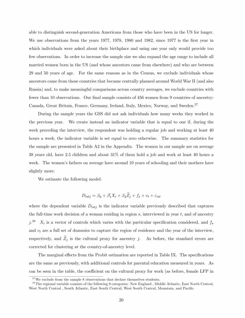
The marginal effects from the Probit estimation are reported in Table IX. The specifications

are the same as previously, with additional controls for parental education measured in years. As

can be seen in the table, the coefficient on the cultural proxy for work (as before, female LFP in

37We exclude from the sample 8 observations that declare themselves students.38The regional variable consists of the following 9 categories: New England , Middle Atlantic, East North Central,

West North Central , South Atlantic, East South Central, West South Central, Mountain, and Pacific.

20

1950) remains basically constant, positive, and statistically significant for all specifications, with

or without parental education. The education of a woman’s father enters negative and marginally

significant in the full specification, whereas the mother’s education is always insignificant. As the

GSS does not report the income of the spouse but only that of the respondent’s and the family,

for our full specification we construct the husband’s income by subtracting the woman’s income

from the family’s total income.39

Table IX allows us to conclude that culture appears to play a quantitatively important role

even after controlling for parental education.40 A one standard deviation increase in female LFP

in 1950 is associated with a 4.4 percentage point increase in the probability that a woman works

full time. Since the predicted value of this probability, calculated at the sample mean, is 28.1

percent, this increase brings the probability of working full time to 32.5 percent.41

A drawback of the GSS analysis is that our sample only includes 9 countries rather than the 25

in our main sample and that our sample size is significantly smaller. An alternative to controlling

for parental human capital directly is to instead use the average education of immigrants who

were in the United States in the 1940s (and whose age makes them likely to be the parents of

the women we observe in the 1970 Census) as a proxy for parental education. This variable also

serves as a measure of the "quality" of the ethnic network that an individual may face. We next

turn to this analysis.

6.2. Ethnic Human Capital

As shown by George Borjas in a number of papers (1992,1995), aggregate ethnic variables may

help explain individual outcomes such as education or earnings. In particular, Borjas has shown

that the earnings of children of immigrants are affected not only by parental earnings (as in the

usual models of intergenerational income mobility), but also by the mean earnings of the ethnic

group in the parents’ generation. In his 1995 paper, he finds that the level of ethnic human

capital (as measured by average wages or average education for immigrant men in the 1940

Census) and neighborhood characteristics help explain the educational attainment and wages of

39Family income is total family income, from all sources in the previous year and before taxes. Respondent’sincome is labor earnings in the previous year before taxes and other deductions. Family and respondent’s incomeson 1972-1993 surveys are in constant dollars (base = 1986). These variables are based on categorical mid-pointsand imputations. For details see GSS Methodological Report No. 64.40We were not able to repeat the same set of exercises for fertility since, once we include the husband’s charac-

teristics, the sample size is reduced and TFR 1950 is no longer significant independently of whether we control forparental education.41The standard deviation of female labor force participation across the 9 countries in the GSS sample is 6.3, with

a mean of 26.4.

21

second generation men aged 18-64 in the 1970 Census. Borjas also used the NLSY which allowed

him to control for parental education directly and found that ethnic human capital still mattered.

Borjas interprets his results as showing that there are ethnic externalities in the human-capital

process.42

In this section we examine the effect of the average education of the immigrant group (ethnic

human capital) in 1940 on a woman’s work and fertility decisions. By including this variable in

our analysis, we will have a proxy both for parental human capital and, to some extent, for the

human capital embodied in the woman’s ethnic network.

To construct a measure of ethnic human capital, we use the 1940 Census to calculate the

average years of education for all individuals not in group quarters who are between the ages

of 25 and 44 and who were born in one of the twenty five countries of our sample. We select

individuals in this age range as it corresponds roughly to the age interval in which we would find

the parents of the women in our sample. We end up with a sample of 26,247 individuals and

many observations per country.43 Across individuals, the average education is 7.9 years; across

countries of ancestry, the average is 7.8 years with a standard deviation of 1.9 years. See Table

1 for the average education of immigrants, reported by country of ancestry.

The results obtained from including this variable (denoted Human Capital 1940) in our

regression analysis are given in Tables X and XI, for work and fertility respectively. Note that

1940 human capital is never significant in explaining fertility, neither on its own nor when combined

with our cultural proxy—TFR 1950. The effect of TFR 1950 remains positive and statistically

significant; its quantitative effect is similar to that found before. Human Capital 1940 does,

however, help to explain the amount worked by women, both on its own (though only in the full

specification in column (v)) and combined with LFP 1950. Note that when we include 1940

human capital, the coefficient on LFP 1950 remains positive and significant though its magnitude

decreases, indicating that countries with higher female LFP also tended to have emigrants with

higher human capital. This could matter, as indicated previously, either because formal education

does not capture all of women’s human capital or because the human capital embodied in ethnic

networks matters to the probability that an individual works, and thus the 1940 human capital

variable captures some component of parental or neighborhood ethnic human capital.

An alternative measure of ethnic network quality would be given by the human capital

42Whether he thinks of these as being strictly economic or having a cultural component, however, is not clear.43All countries have over 75 observations with the exception of Lebanon for which we have only 4.

22

embodied in other second-generation individuals from the same country of ancestry who belong

to a similar age group as the women in our sample. In this case, the network would consist of

individuals within the same generation rather than across generations as previously. Tables XII

and XIII repeat the same exercise as in Tables X and XI, but this time controlling for Human

Capital 1970, i.e., the average years of education of second-generation immigrants from the same

country of ancestry who are between the ages of twenty five and forty five.44 We find a very

similar pattern of results as for 1940 Human Capital, with the exception that human capital in

1970 is not significant when female LFP 1950 is included in the full specification for the work

regression.45

We also explored the robustness of our results to other measures of ethnic human capital

both for 1940 and 1970. In particular, we used average education only of women, only of men

and, for 1940, also only of married women and only of married men. Our results were very similar

across all cases.

6.3. Men and Culture

In this section we conduct what we consider a critical test of the validity of our hypothesis. In

particular, we ask whether our proxy for cultural attitudes towards women working (female LFP

1950) is able to positively and significantly explain how much second-generation men work in

the United States in 1970. If the explanatory power of our proxy is truly coming from culture

rather than from some omitted correlated variable, then the cultural proxy should not have

similar explanatory power for how much men work. That is, unless something like a household

substitution effect is in operation, there is no a priori reason to expect that beliefs as to the proper

role of women in society should explain how much men work.46 As we show below, our hypothesis

passes this test with flying colors. The same asymmetry, however, should not extend necessarily

to our cultural proxy for children. The number of children in the household is common to both

spouses and thus there may be a cultural attitude towards family size that is common for men and

women. Consequently, one may well expect the cultural proxy (TFR 1950) to capture cultural

preferences towards family size and hence help explain the number of children of men and women.

44See Table I for the value of this variable by country. The mean is 12.3 years with a standard deviation of 0.86.45Note that the dependent variable in the work regression is now hours worked. We could not use weeks worked

as human capital 1970 and LFP 1950 are highly correlated (over 0.7) and they both became insignificant (and theadjusted R squared decreased) when they were both included in the same specification for weeks worked.46The cultural proxy could, however, have a negative and significant coefficient if individuals tend to marry others

within their own ancestry and if men whose wives work less tend to work more themselves to increase householdincome. This, however, as we show, is not the case.

23

This is indeed the case, as we show below.

We select the men for our sample with the same procedure used to construct our sample of

women. That is, we select all married men, age 30-40, born in the US, and not living on farms

or group quarters and not working in agriculture. From this group we exclude all men whose

fathers were born in the US (leaving us with approximately 11% of the sample), eliminate those

whose replies were not countries, and exclude the European centrally-planned economies. Lastly,

we drop those countries with fewer than 15 observations. Our final sample of men has 6710

observations and the same 25 countries as for our main sample of women.

In 1970, the men in our sample were working on average 41.3 hours a week (with a standard

deviation of 14.9 hours) and 49.0 weeks a year (with a standard deviation of 7 weeks). As in

the case of women, the individual means are basically the same as those obtained by averaging

observations by country of ancestry, whereas the standard deviations are significantly smaller for

the latter (3.1 and 0.9 for hours and weeks respectively). Interestingly, the men in our sample

(unlike their female counterparts) work slightly more than men whose fathers were born in the

US (the latter worked on average 40.5 hours per week and 48.7 weeks per year with standard

deviations of 16.1 hours and 7.7 weeks respectively).

In order to easily test whether the coefficients on the cultural proxies are significantly different

for men and women, we combine the sample of 6710 men with the sample of 6774 women for a

total of 13,484 individuals and 25 countries. Our regressions now include a dummy variable for

each gender which we in addition interact with all explanatory variables in all specifications.

We report our results both for weeks and for hours worked in Table XIV. We are particu-

larly interested in hours as, especially for men, weeks worked may not capture the intensity of

an individual’s work efforts. The main variables of interest are Female x LFP 1950 and Male x

LFP 1950. Note that when the observation is a woman we use her father’s country of birth to

assign ancestry and if the observation is a man we use his father’s country of birth. As shown in

the table, the culture proxy is never significant in explaining how much men work once individual

characteristics are included in the work regression. As before, however, the culture proxy is posi-

tively and significantly associated with how much women work in all specifications. Furthermore,

we can reject at the 1% and 5% levels for weeks and hours respectively, the hypothesis that the

coefficients on the culture proxy for men and women are equal. It is interesting to note that

a wife’s education (coefficients not shown) has the opposite effect on the work behavior of her

spouse (positive) than a husband’s education has on the work behavior of his spouse (negative).

24

The effect of spouse’s income is negative across genders.

While our ability to reject the hypothesis that the culture proxy variable helps explain how

much men work is not definitive evidence in favor our thesis, it does significantly decrease the

probability that other omitted variables are driving our results. It also points to the fact that,

if there is some omitted variable that is positively correlated to female LFP 1950, it would most

likely have explanatory power for women’s labor supply but not for men’s. It is not easy to

imagine what such a variable might be such that did not also contain a significant component

of culture. For example, this variable may be picking up the possibility that parents from low

female LFP countries invest less in unobserved human capital for their daughters relative to their

sons than parents from high female LFP countries, precisely the type of cultural explanation we

are attempting to explore. That is, although one may conjecture that this asymmetric behavior

may have existed for purely economic reasons in the country of ancestry, the fact that this pattern

is repeated in a different economic and institutional context makes it likely that this behavior also

reflects important beliefs about the role of women.

Lastly, we examine whether the cultural proxy for family size, TFR in 1950, has explanatory

power for men as well as for women. We now use the number of children in the household as the

dependent variable, as this allows us to treat both men and women symmetrically. The results

of this analysis are presented in Table XV.

As shown in the table, the cultural proxy for children is positive and significant for both

women and men. The coefficient is larger for women than for men (the hypothesis that they are

equal can be rejected at the 1% level), which may indicate that women may respond more to the

cultural background of their parents (or perhaps of their neighborhood) than men.47 Interestingly,

unlike for the case of work, the number of children in the household is associated negatively with

the level of the spouse’s education for both genders. The effect of a spouse’s income, however,

is now asymmetric, though this is not surprising given traditional gender roles. A man whose

wife’s total income is high tends to have fewer children; a woman whose husband’s total income

is high tends to have more children.

7. Her or His Culture?

A married woman’s work and fertility outcomes are likely to be influenced not only by the factors

that we have already explored—her age and education, her beliefs as embodied in the cultural

47Whether women and men "assimilate" at a different rate is an interesting question to pursue in future research.

25

proxies, and her husband’s characteristics, but also by the beliefs—by the culture—of her husband.

In this section we wish to explore whether the husband’s cultural beliefs as to the role of women

and family size affect his wife’s work and fertility outcomes. Of course, a woman’s culture and

that of her husband’s are unlikely to be random: A woman who would like to work or would prefer

a larger family is presumably more likely to marry a man who would be in agreement with these

choices. Nonetheless, it is of interest to ask whether it is her culture or her husband’s culture or

both that matter to these outcomes.48

In order to study whose culture matters to a woman’s work and fertility outcomes, we include

cultural proxies for both the woman and her husband, in each case assigned by the country of

birth of each spouses’ father. Note that many women will be married to men whose fathers were

born in the US. To these men, therefore, we must associate US female LFP and TFR in 1950.

In order to not have an asymmetric sample in which the US variables would only appear as a

cultural proxy when associated with a woman’s husband, we expand our sample to include women

whose fathers were born in the US but whose fathers-in-law are foreign born. We follow the same

procedure we described earlier: we drop those women whose father-in-law is from a European

centrally planned economy or from a country for which we have fewer than 15 observations. Our

final sample consists of 12,060 married women and 26 countries (including US).49 In this sample,

32.6% of women are married to men whose father was born in the US (and thus these women’s

father was born elsewhere); 47.6% of the women have fathers born in the US (and hence they are

married to men with foreign born fathers). The remaining 19.7% of women and their husbands

both have fathers born outside the US. Only 13.7% of the couples in our sample share the same

culture (i.e., have fathers born in the same country), though this is due to the fact that we have

omitted those women with US fathers and US fathers-in-law. If we were to restrict our attention

to couples in which neither spouse has a father born in the US, then 69.4% of these share the

same culture.

To study the effect of the two spouses’ cultures, we distinguish between couples who share

identical cultures (i.e., their fathers were born in the same country) from those with different

cultures. We create two dummy variables: Same (for same culture) and Not Same (for different

cultures) and interact these with the cultural proxies. It should be noted that the number of

48Once one leaves the unitary household model, there is no reason to believe that husband and wives necessarilyshare the same preferences over outcomes (see, e.g., Lundberg and Pollak (1996)).49Another way of thinking about our sample selection is that from the universe of married women born in the US

and between the ages of 30-40, we have eliminated those women who have both a US born father and a US bornfather-in-law.

26

https://www.researchgate.net/publication/4902063_Bargaining_and_Distribution_in_Marriage?el=1_x_8&enrichId=rgreq-de211374d6dfda50bcaa5a39b0707b21-XXX&enrichSource=Y292ZXJQYWdlOzUwMDk1Njc7QVM6MTA2NjIyNjE3NjUzMjUxQDE0MDI0MzIyMjE5MTc=

observations for same culture is relatively small (1653). The results of our regression analysis are

reported for the full specification in Table XVI.

The first column in Table XVI reports the results for weeks worked using only the wife’s

cultural proxy for work. As before, it is positive and statistically significant (for Not Same).

The next column uses only the husband’s cultural proxy which is also positive and statistically

significant. The third column uses both proxies. Interestingly, the coefficient on the husband’s

cultural proxy is larger and more significant than that of his wife’s (which is no longer significant).

Furthermore, in this last specification, the coefficient on the cultural proxy when the culture of

the two spouses is the same is significant (at the 10% level) and larger than either of the two

different cultures coefficients.

Columns (iv)-(vi) in Table XVI repeat the same specifications for fertility. The cultural proxy

is positive and significant when it is the wife’s, the husband’s, and when both are simultaneously

included. When the wife and husband share the same culture, the cultural proxy is also positive

and significant, this time in all three specifications. The coefficients for each spouse separately

are basically equal as are the coefficients for each spouse when they are entered jointly in the final

specification. In this last specification, the sum of the coefficients on the wife’s and the husband’s

cultural proxies essentially sum to the coefficient on cultural proxy when the spouses share the

same culture.

We have also experimented with restricting our sample to the subset of women who have

neither a US father nor a US father-in-law.50 The results are similar to the ones above except

that for the work regressions the cultural proxy when the couple shares the same culture is now

much larger, positive, and significant for all three specifications.

8. Cultural Transmission

In this section we briefly explore the role of neighborhood composition in cultural transmission.

An individual’s neighborhood may play an important role in transmitting and preserving a set

of beliefs, independently of the human capital embodied in an individual’s ethnic network. A

neighborhood that has a relatively high proportion of individuals from the same ancestry may

help preserve that country’s culture by punishing behavior that is different than the norm (by,

for example, ostracizing the deviant individual). It may also keep the culture of the country of

ancestry alive by providing role models and diffusing specific beliefs about how individuals, and

50There are 2381 such observations.

27

in particular women, should act. In this section we partially explore the role of neighborhoods

in cultural transmission and preservation by investigating how the propensity of an ethnic group

to cluster in the same neighborhood affects the impact of culture. The hypothesis is that the

greater is the proportion of an ethnic group in a neighborhood, the larger will be the effect of the

cultural proxies on individual behavior. Note that this is a different type of "ethnic externality"

than those explored by Borjas in his work. Here it is not the education of the ethnic group that

is an input into the production of an individual’s human capital, but rather the greater presence

of this group in a community that facilitates the transmission and preservation of a particular set

of beliefs.

To explore the role of ethnic density, we turn to data provided in Borjas (1995). Borjas uses

the 1/100 Neighborhood File of the 1970 US Census to study the effect of ethnicity and neigh-

borhoods on intergenerational transmission. He calculates the extent of residential segregation

for both first and second-generation Americans by estimating the proportion of the respondent’s

neighborhood that is of the same ethnicity and averaging this number across respondents.51 We

use Borjas’ estimates of residential segregation for second-generation Americans to attach an av-

erage ethnic density to each country of ancestry.52 These numbers are reported by country of

ancestry in Table I.

As can be seen in Table I, on average, second-generation Americans typically live in neigh-

borhoods where the density of their own ethnic group is 4.3% with a standard deviation of 4.5%

(i.e., the average second-generation American resides in a neighborhood in which 4.3% of the

community is from the same ethnic group). Mexicans, Italians, and Japanese live in ethnically

dense neighborhoods (respectively, 18.1, 12.1 and 12.6), whereas Turks, French, and Lebanese

live in neighborhoods with low ethnic density (0.3, 0.3, and 0.4, respectively). Note that the

ethnic density number depends both on the extent to which members of an ethnic group cluster

into the same neighborhoods and how large that ethnic group is in the population (since if the

ethnic group is not large, then even if they tended to cluster, this could show up as a low density

number). The rank correlation of the number of observations by country of ancestry in Table I

and ethnic density is 0.5, showing that both elements probably play a role. In any case, from

the perspective of cultural transmission, it may not matter which variable is the source of ethnic

51See Borjas (1995), Table 2.52Borjas does not include Spain, so individuals from this country of ancestry are excluded in the analysis that

follows. He also has separate entries for England, Wales, and Scotland which we aggregate to one U.K. value byweighing each separate density figure by the proportion of U.K. observations in our sample that come from each ofthese three countries.

28

density.

In order to explore the effect of ethnic density, we include density, the cultural proxy, and

density interacted with the culture proxy in our regression analysis both separately and jointly.

Tables XVII and Table XVIII report the effects for hours worked and fertility respectively.53

Across all specifications, density is only significant if the culture proxy variable is also included.

The last column in each table reports the coefficients for the full specification. Note that the

interaction of culture and density is positive and significant. Moreover, the full marginal effects of

female LFP 1950 and TFR 1950 remain positive and significant whereas the full marginal effect of

density is insignificant when evaluated at the mean. A one standard deviation increase in female

LFP 1950 is associated with a 0.76 increase in hours worked (evaluated at the mean of density);

a one standard deviation increase in TFR 1950 is associated with a 0.19 increase in the number

of children.

From the above we conclude that the degree to which ethnic groups cluster in the same

neighborhoods appears to be an important mechanism in maintaining culture: the greater is the

average density of an ethnic group, the greater is the impact of culture on a woman’s work and

fertility outcomes.54

9. Conclusion

This paper argues that culture matters to important economic outcomes, namely, female work and

fertility. We show that female LFP and TFR in 1950 by country of ancestry, our cultural proxies,

are economically and statistically significant in explaining how much women work and how many

children they have. We also examine the most likely suspects that could be responsible for our

results. In particular, we have shown that neither unobserved human capital nor network quality

are likely to be the driving forces. On the other hand, we find that the average propensity of

an ethnic group to cluster in the same neighborhood magnifies the impact of the cultural proxies

on work and fertility, which is consistent with our theory that cultural transmission through

the family and neighborhood matters. Perhaps most convincingly of all, we have shown that

the cultural proxy for female work has no explanatory power for the work behavior of a similar

sample of men (in line with our hypothesis that this variable reflects cultural attitudes towards

women in society), whereas the cultural proxy for fertility is significant in explaining the number

53Similar results are obtained for weeks worked.54Whether this has positive or negative welfare effects depends on one’s view about the validity of the underlying

beliefs.

29

of children they have.

There are, of course, other interpretations of the empirical evidence other than ours of culture.

For example, if household skills are transmitted primarily from mothers to daughters and if these

are higher for mothers who do not work, than the traditional comparative advantage argument

may help explain why the daughters of women from low female LFP countries tend to work less.

This alternative hypothesis, however, would not explain why the impact of the cultural proxy is

stronger the greater is the propensity of the ethnic group to cluster into neighborhoods.

Another hypothesis is that there are varying degrees of discrimination in the US labor market

that (negatively) correlate with female LFP in the country-of-ancestry. We do not think that

such a correlation is very plausible especially since most of our sample consists of women from

European countries of ancestry. Furthermore, we do not see this pattern for men by country of

ancestry. This implies that if discrimination (in hiring) is responsible for the observed pattern of

results, it would have to be faced only by the women and not by the men from these countries,

which seems rather implausible.

We think that our estimates of the quantitative impact of culture are likely to underestimate

its true importance. Indeed, we find it telling that despite the fact that we study the work and

fertility behavior of second-generation immigrants to the US (who are likely never to have set

foot in their father’s country of ancestry), and despite the fact that we control for most of the

indirect effects of culture (a woman’s education and her husband’s age, education, and income),

we nonetheless find the direct effect of our cultural proxies to be significant. We think, therefore,

that culture is likely to play an important role in explaining the large variation across time and

countries in women’s work and fertility. Moreover, there is no reason to believe that culture’s

impact is restricted to the variables we studied. Culture is also likely to play a role in explaining

cross-country variation in other individual economic outcomes such as entrepreneurial activity,

creativity, and physical and human capital accumulation. These, similarly to female labor force

participation and fertility, are all likely to affect aggregate outcomes such as per capita GDP,

growth, or inequality. Culture, therefore, is too important an area for economists to ignore.

30

References

[1] Acemoglu, D., S. Johnson, and J. Robinson (2004), “Institutions as the Fundamental Cause

of Long-Run Growth,” mimeo, MIT, April 2004.

[2] Antecol, H. (2000), “An Examination of Cross-Country Differences in the Gender Gap in

Labor Force Participation Rates”, Labour Economics 7, 409-426.

[3] _______ (2001) “Why Is There Interethnic Variation in the Gender Wage Gap? The

Role of Cultural Factors”,. Journal of Human Resources 36(1), 119-143.

[4] Barro, R. and R. McCleary (2003) “Religion and Economic Growth”, NBER Working Paper

No. 9682.

[5] Bisin, A. and T. Verdier (2000), “Beyond the Melting Pot: Cultural Transmission, Marriage,

and the Evolution of Ethnic and Religious Traits”, Quarterly Journal of Economics, 115(3),

955-988.

[6] Blau, F.D. (1992), “The Fertility of Immigrant Women: Evidence from High Fertility Source

Countries”, in: Borjas, G.J., Freeman, R. (Eds.), Immigration and the Workforce: Economic

Consequences for the United States and Source Areas, University of Chicago Press, Chicago,

93-133.

[7] Borjas, G. (1992), “Ethnic Capital and Intergenerational Mobility”, Quarterly Journal of

Economics, 107 (1), 123-50.

[8] _______ (1995), “Ethnicity, Neighborhoods, and Human-Capital Externalities”, Ameri-

can Economic Review, 85(3), 365-390.

[9] Carroll, C., B. Rhee and C. Rhee (1994), “Are there Cultural Effects on Saving? Some

Cross-Sectional Evidence”, Quarterly Journal of Economics, 109(3), 685-99.

[10] Cole, H., G. Mailath, and A. Postlewaite (1992), “Social Norms, Savings Behavior and

Growth”, Journal of Political Economy, 100, 1092-1125.

[11] Davis, J., T. Smith and P. Marsden (1999), General Social Surveys, 1972-1998: Cumulative

Codebook, Chicago, NORC.

31

https://www.researchgate.net/publication/4901296_Ethnicity_Neighborhoods_and_Human-Capital_Externalities?el=1_x_8&enrichId=rgreq-de211374d6dfda50bcaa5a39b0707b21-XXX&enrichSource=Y292ZXJQYWdlOzUwMDk1Njc7QVM6MTA2NjIyNjE3NjUzMjUxQDE0MDI0MzIyMjE5MTc=

https://www.researchgate.net/publication/4901296_Ethnicity_Neighborhoods_and_Human-Capital_Externalities?el=1_x_8&enrichId=rgreq-de211374d6dfda50bcaa5a39b0707b21-XXX&enrichSource=Y292ZXJQYWdlOzUwMDk1Njc7QVM6MTA2NjIyNjE3NjUzMjUxQDE0MDI0MzIyMjE5MTc=







https://www.researchgate.net/publication/5197654_Religion_and_Economic_Growth?el=1_x_8&enrichId=rgreq-de211374d6dfda50bcaa5a39b0707b21-XXX&enrichSource=Y292ZXJQYWdlOzUwMDk1Njc7QVM6MTA2NjIyNjE3NjUzMjUxQDE0MDI0MzIyMjE5MTc=

https://www.researchgate.net/publication/5197654_Religion_and_Economic_Growth?el=1_x_8&enrichId=rgreq-de211374d6dfda50bcaa5a39b0707b21-XXX&enrichSource=Y292ZXJQYWdlOzUwMDk1Njc7QVM6MTA2NjIyNjE3NjUzMjUxQDE0MDI0MzIyMjE5MTc=



https://www.researchgate.net/publication/24103750_Social_Norms_Savings_Behavior_and_Growth?el=1_x_8&enrichId=rgreq-de211374d6dfda50bcaa5a39b0707b21-XXX&enrichSource=Y292ZXJQYWdlOzUwMDk1Njc7QVM6MTA2NjIyNjE3NjUzMjUxQDE0MDI0MzIyMjE5MTc=

https://www.researchgate.net/publication/24103750_Social_Norms_Savings_Behavior_and_Growth?el=1_x_8&enrichId=rgreq-de211374d6dfda50bcaa5a39b0707b21-XXX&enrichSource=Y292ZXJQYWdlOzUwMDk1Njc7QVM6MTA2NjIyNjE3NjUzMjUxQDE0MDI0MzIyMjE5MTc=

https://www.researchgate.net/publication/24091460_Are_There_Cultural_Effects_on_Saving_Some_Cross-Sectional_Evidence?el=1_x_8&enrichId=rgreq-de211374d6dfda50bcaa5a39b0707b21-XXX&enrichSource=Y292ZXJQYWdlOzUwMDk1Njc7QVM6MTA2NjIyNjE3NjUzMjUxQDE0MDI0MzIyMjE5MTc=

https://www.researchgate.net/publication/24091460_Are_There_Cultural_Effects_on_Saving_Some_Cross-Sectional_Evidence?el=1_x_8&enrichId=rgreq-de211374d6dfda50bcaa5a39b0707b21-XXX&enrichSource=Y292ZXJQYWdlOzUwMDk1Njc7QVM6MTA2NjIyNjE3NjUzMjUxQDE0MDI0MzIyMjE5MTc=

https://www.researchgate.net/publication/46552471_Why_Is_There_Interethnic_Variation_in_the_Gender_Wage_Gap_The_Role_of_Cultural_Factors?el=1_x_8&enrichId=rgreq-de211374d6dfda50bcaa5a39b0707b21-XXX&enrichSource=Y292ZXJQYWdlOzUwMDk1Njc7QVM6MTA2NjIyNjE3NjUzMjUxQDE0MDI0MzIyMjE5MTc=

https://www.researchgate.net/publication/46552471_Why_Is_There_Interethnic_Variation_in_the_Gender_Wage_Gap_The_Role_of_Cultural_Factors?el=1_x_8&enrichId=rgreq-de211374d6dfda50bcaa5a39b0707b21-XXX&enrichSource=Y292ZXJQYWdlOzUwMDk1Njc7QVM6MTA2NjIyNjE3NjUzMjUxQDE0MDI0MzIyMjE5MTc=

https://www.researchgate.net/publication/5067423_Beyond_the_Melting_Pot_Cultural_Transmission_Marriage_and_the_Evolution_of_Ethnic_and_Religious_Traits?el=1_x_8&enrichId=rgreq-de211374d6dfda50bcaa5a39b0707b21-XXX&enrichSource=Y292ZXJQYWdlOzUwMDk1Njc7QVM6MTA2NjIyNjE3NjUzMjUxQDE0MDI0MzIyMjE5MTc=



https://www.researchgate.net/publication/4756101_Institutions_as_the_Fundamental_Cause_of_Long-Run_Growth?el=1_x_8&enrichId=rgreq-de211374d6dfda50bcaa5a39b0707b21-XXX&enrichSource=Y292ZXJQYWdlOzUwMDk1Njc7QVM6MTA2NjIyNjE3NjUzMjUxQDE0MDI0MzIyMjE5MTc=

https://www.researchgate.net/publication/4756101_Institutions_as_the_Fundamental_Cause_of_Long-Run_Growth?el=1_x_8&enrichId=rgreq-de211374d6dfda50bcaa5a39b0707b21-XXX&enrichSource=Y292ZXJQYWdlOzUwMDk1Njc7QVM6MTA2NjIyNjE3NjUzMjUxQDE0MDI0MzIyMjE5MTc=

[12] Elster, J. “Social Norms and Economic Theory,” Journal of Economic Perspectives, 3(4),

1989, 99-117.

[13] Fernández, R., A. Fogli, and C. Olivetti (2004), “Mothers and Sons: Preference Formation

and Female Labor Force Dynamics”, Quarterly Journal of Economics, 119 (4), 1249-1299.

[14] Fernández, R. N. Guner, and J. Knowles (2005, “Love and Money: A Theoretical and Em-

pirical Analysis of Household Sorting and Inequality,” Quarterly Journal of Economics, 120

(1), 273-344.

[15] Giuliano, P.(2004), “On the Determinants of Living Arrangements in Western Europe: Does

Cultural Origin Matter?”, mimeo, U.C. Berkeley.

[16] Goldin, C. (1990), Understanding the Gender Gap: An Economic History of American

Women, New York: Oxford University Press.

[17] Guinnane, T., C. Moehling, and C. O Grada (2002), “The Fertility of the Irish in America

in 1910”, mimeo, Yale University.

[18] ILO (1988), Current International Recommendations on Labour Statistics, Geneva.

[19] Landes, D. (1998), The Wealth and Poverty of Nations, New York, W.W. Norton.

[20] Levine, D. (1993), “The Effect of Non-Traditional Attitudes on Married Women’s Labor

Supply”, Journal of Economic Psychology, 14, 665-679.

[21] Lundberg, S. and R. Pollak (1996), “Bargaining and Distribution in Marriage,” Journal of

Economic Perspectives, 10 (4), 139-158

[22] Maddison, A. (1995), Monitoring The World Economy 1820-1992, Paris, Organisation for

Economic Co-Operation and Development.

[23] Pencavel, J. (1998), “The Market Work Behavior and Wages of Women, 1975-94,” Journal

of Human Resources, 38(4), 771-804.

[24] Persson, T. and G. Tabellini (2003), The Economic Effect of Constitutions, MIT Press:

Cambridge.

[25] Putnam, R. (2000), Bowling Alone: The Collapse and Revival of American Community,

Simon and Schuster.

32



https://www.researchgate.net/publication/24091892_Love_and_Money_A_Theoretical_and_Empirical_Analysis_of_Household_Sorting_and_Inequality?el=1_x_8&enrichId=rgreq-de211374d6dfda50bcaa5a39b0707b21-XXX&enrichSource=Y292ZXJQYWdlOzUwMDk1Njc7QVM6MTA2NjIyNjE3NjUzMjUxQDE0MDI0MzIyMjE5MTc=



https://www.researchgate.net/publication/5012044_The_Fertility_of_the_Irish_in_America_in_1910?el=1_x_8&enrichId=rgreq-de211374d6dfda50bcaa5a39b0707b21-XXX&enrichSource=Y292ZXJQYWdlOzUwMDk1Njc7QVM6MTA2NjIyNjE3NjUzMjUxQDE0MDI0MzIyMjE5MTc=

https://www.researchgate.net/publication/5012044_The_Fertility_of_the_Irish_in_America_in_1910?el=1_x_8&enrichId=rgreq-de211374d6dfda50bcaa5a39b0707b21-XXX&enrichSource=Y292ZXJQYWdlOzUwMDk1Njc7QVM6MTA2NjIyNjE3NjUzMjUxQDE0MDI0MzIyMjE5MTc=







https://www.researchgate.net/publication/4726728_Social_Norms_and_Economic_Theory?el=1_x_8&enrichId=rgreq-de211374d6dfda50bcaa5a39b0707b21-XXX&enrichSource=Y292ZXJQYWdlOzUwMDk1Njc7QVM6MTA2NjIyNjE3NjUzMjUxQDE0MDI0MzIyMjE5MTc=

https://www.researchgate.net/publication/4726728_Social_Norms_and_Economic_Theory?el=1_x_8&enrichId=rgreq-de211374d6dfda50bcaa5a39b0707b21-XXX&enrichSource=Y292ZXJQYWdlOzUwMDk1Njc7QVM6MTA2NjIyNjE3NjUzMjUxQDE0MDI0MzIyMjE5MTc=





https://www.researchgate.net/publication/243779723_Monitoring_the_World_Economy_1820-1992?el=1_x_8&enrichId=rgreq-de211374d6dfda50bcaa5a39b0707b21-XXX&enrichSource=Y292ZXJQYWdlOzUwMDk1Njc7QVM6MTA2NjIyNjE3NjUzMjUxQDE0MDI0MzIyMjE5MTc=

https://www.researchgate.net/publication/243779723_Monitoring_the_World_Economy_1820-1992?el=1_x_8&enrichId=rgreq-de211374d6dfda50bcaa5a39b0707b21-XXX&enrichSource=Y292ZXJQYWdlOzUwMDk1Njc7QVM6MTA2NjIyNjE3NjUzMjUxQDE0MDI0MzIyMjE5MTc=

https://www.researchgate.net/publication/23573672_The_Economic_Effect_of_Constitutions?el=1_x_8&enrichId=rgreq-de211374d6dfda50bcaa5a39b0707b21-XXX&enrichSource=Y292ZXJQYWdlOzUwMDk1Njc7QVM6MTA2NjIyNjE3NjUzMjUxQDE0MDI0MzIyMjE5MTc=

https://www.researchgate.net/publication/23573672_The_Economic_Effect_of_Constitutions?el=1_x_8&enrichId=rgreq-de211374d6dfda50bcaa5a39b0707b21-XXX&enrichSource=Y292ZXJQYWdlOzUwMDk1Njc7QVM6MTA2NjIyNjE3NjUzMjUxQDE0MDI0MzIyMjE5MTc=

https://www.researchgate.net/publication/200033199_The_Wealth_and_Poverty_of_Nations_NY_Norton?el=1_x_8&enrichId=rgreq-de211374d6dfda50bcaa5a39b0707b21-XXX&enrichSource=Y292ZXJQYWdlOzUwMDk1Njc7QVM6MTA2NjIyNjE3NjUzMjUxQDE0MDI0MzIyMjE5MTc=

[26] Reimers, C.(1985), “Cultural Differences in Labor Force Participation Among Married

Women”, American Economic Review Papers and Proceedings, 75(2), 251-255.

[27] Stigler, G. and G. Becker (1977), “De Gustibus Non Est Disputandum”, American Economic

Review, 67(2), 76-90.

[28] Vella, F. (1994), “Gender Roles and Human Capital Investment: The Relationship between

Traditional Attitudes and Female Labour Force Performance”, Economica, 61, 191-211.

[29] Weil, D. (2004), Economic Growth, Addison Wesley

33

https://www.researchgate.net/publication/4889553_Gender_Roles_and_Human_Capital_Investment_The_Relationship_between_Traditional_Attitudes_and_Female_Labour_Market_Performance?el=1_x_8&enrichId=rgreq-de211374d6dfda50bcaa5a39b0707b21-XXX&enrichSource=Y292ZXJQYWdlOzUwMDk1Njc7QVM6MTA2NjIyNjE3NjUzMjUxQDE0MDI0MzIyMjE5MTc=

https://www.researchgate.net/publication/4889553_Gender_Roles_and_Human_Capital_Investment_The_Relationship_between_Traditional_Attitudes_and_Female_Labour_Market_Performance?el=1_x_8&enrichId=rgreq-de211374d6dfda50bcaa5a39b0707b21-XXX&enrichSource=Y292ZXJQYWdlOzUwMDk1Njc7QVM6MTA2NjIyNjE3NjUzMjUxQDE0MDI0MzIyMjE5MTc=

https://www.researchgate.net/publication/4980250_Cultural_Differences_in_Labor_Force_Participation_Among_Married_Women?el=1_x_8&enrichId=rgreq-de211374d6dfda50bcaa5a39b0707b21-XXX&enrichSource=Y292ZXJQYWdlOzUwMDk1Njc7QVM6MTA2NjIyNjE3NjUzMjUxQDE0MDI0MzIyMjE5MTc=

https://www.researchgate.net/publication/4980250_Cultural_Differences_in_Labor_Force_Participation_Among_Married_Women?el=1_x_8&enrichId=rgreq-de211374d6dfda50bcaa5a39b0707b21-XXX&enrichSource=Y292ZXJQYWdlOzUwMDk1Njc7QVM6MTA2NjIyNjE3NjUzMjUxQDE0MDI0MzIyMjE5MTc=

https://www.researchgate.net/publication/4745334_De_Gustibus_Non_Est_Disputandum?el=1_x_8&enrichId=rgreq-de211374d6dfda50bcaa5a39b0707b21-XXX&enrichSource=Y292ZXJQYWdlOzUwMDk1Njc7QVM6MTA2NjIyNjE3NjUzMjUxQDE0MDI0MzIyMjE5MTc=

https://www.researchgate.net/publication/4745334_De_Gustibus_Non_Est_Disputandum?el=1_x_8&enrichId=rgreq-de211374d6dfda50bcaa5a39b0707b21-XXX&enrichSource=Y292ZXJQYWdlOzUwMDk1Njc7QVM6MTA2NjIyNjE3NjUzMjUxQDE0MDI0MzIyMjE5MTc=

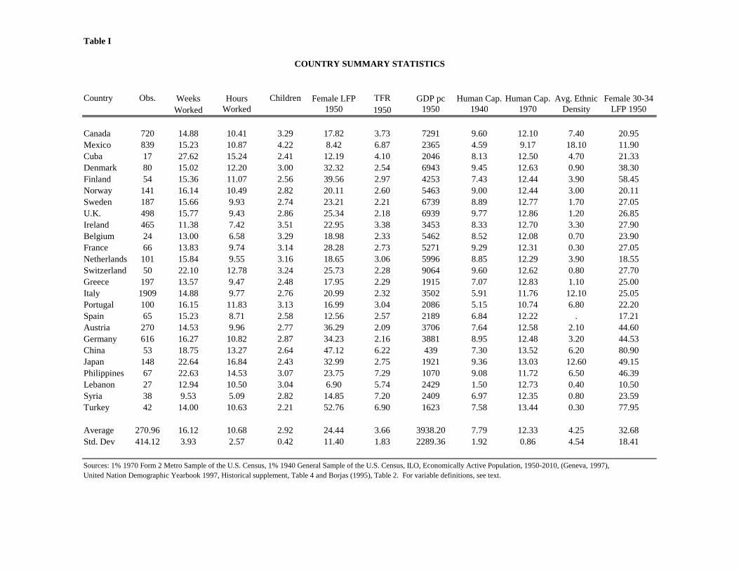
Table I

Country Obs. Weeks Hours Children Female LFP TFR GDP pc Human Cap. Human Cap. Avg. Ethnic Female 30-34Worked Worked 1950 1950 1950 1940 1970 Density LFP 1950

Canada 720 14.88 10.41 3.29 17.82 3.73 7291 9.60 12.10 7.40 20.95Mexico 839 15.23 10.87 4.22 8.42 6.87 2365 4.59 9.17 18.10 11.90Cuba 17 27.62 15.24 2.41 12.19 4.10 2046 8.13 12.50 4.70 21.33Denmark 80 15.02 12.20 3.00 32.32 2.54 6943 9.45 12.63 0.90 38.30Finland 54 15.36 11.07 2.56 39.56 2.97 4253 7.43 12.44 3.90 58.45Norway 141 16.14 10.49 2.82 20.11 2.60 5463 9.00 12.44 3.00 20.11Sweden 187 15.66 9.93 2.74 23.21 2.21 6739 8.89 12.77 1.70 27.05U.K. 498 15.77 9.43 2.86 25.34 2.18 6939 9.77 12.86 1.20 26.85Ireland 465 11.38 7.42 3.51 22.95 3.38 3453 8.33 12.70 3.30 27.90Belgium 24 13.00 6.58 3.29 18.98 2.33 5462 8.52 12.08 0.70 23.90France 66 13.83 9.74 3.14 28.28 2.73 5271 9.29 12.31 0.30 27.05Netherlands 101 15.84 9.55 3.16 18.65 3.06 5996 8.85 12.29 3.90 18.55Switzerland 50 22.10 12.78 3.24 25.73 2.28 9064 9.60 12.62 0.80 27.70Greece 197 13.57 9.47 2.48 17.95 2.29 1915 7.07 12.83 1.10 25.00Italy 1909 14.88 9.77 2.76 20.99 2.32 3502 5.91 11.76 12.10 25.05Portugal 100 16.15 11.83 3.13 16.99 3.04 2086 5.15 10.74 6.80 22.20Spain 65 15.23 8.71 2.58 12.56 2.57 2189 6.84 12.22 . 17.21Austria 270 14.53 9.96 2.77 36.29 2.09 3706 7.64 12.58 2.10 44.60Germany 616 16.27 10.82 2.87 34.23 2.16 3881 8.95 12.48 3.20 44.53China 53 18.75 13.27 2.64 47.12 6.22 439 7.30 13.52 6.20 80.90Japan 148 22.64 16.84 2.43 32.99 2.75 1921 9.36 13.03 12.60 49.15Philippines 67 22.63 14.53 3.07 23.75 7.29 1070 9.08 11.72 6.50 46.39Lebanon 27 12.94 10.50 3.04 6.90 5.74 2429 1.50 12.73 0.40 10.50Syria 38 9.53 5.09 2.82 14.85 7.20 2409 6.97 12.35 0.80 23.59Turkey 42 14.00 10.63 2.21 52.76 6.90 1623 7.58 13.44 0.30 77.95

Average 270.96 16.12 10.68 2.92 24.44 3.66 3938.20 7.79 12.33 4.25 32.68Std. Dev 414.12 3.93 2.57 0.42 11.40 1.83 2289.36 1.92 0.86 4.54 18.41

Sources: 1% 1970 Form 2 Metro Sample of the U.S. Census, 1% 1940 General Sample of the U.S. Census, ILO, Economically Active Population, 1950-2010, (Geneva, 1997),United Nation Demographic Yearbook 1997, Historical supplement, Table 4 and Borjas (1995), Table 2. For variable definitions, see text.

COUNTRY SUMMARY STATISTICS

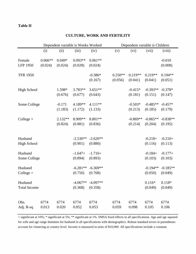
Table II

(i) (ii) (iii) (iv) (v) (vi) (vii) (viii)

Female 0.066** 0.049* 0.093** 0.061** -0.010LFP 1950 (0.024) (0.024) (0.028) (0.024) (0.008)

TFR 1950 -0.386* 0.250** 0.219** 0.219** 0.194**(0.167) (0.056) (0.041) (0.041) (0.051)

High School 1.598* 3.783** 3.651** -0.415* -0.393** -0.378*(0.676) (0.677) (0.643) (0.181) (0.151) (0.147)

Some College -0.171 4.189** 4.111** -0.503* -0.485** -0.457*(1.183) (1.172) (1.133) (0.213) (0.185) (0.179)

College + 2.132** 8.909** 8.801** -0.869** -0.865** -0.838**(0.824) (0.881) (0.836) (0.214) (0.204) (0.195)

Husband -2.530** -2.620** -0.218+ -0.210+High School (0.901) (0.880) (0.116) (0.113)

Husband -1.647+ -1.716+ -0.184+ -0.177+Some College (0.894) (0.893) (0.103) (0.103)

Husband -6.281** -6.369** -0.194** -0.185**College + (0.750) (0.768) (0.050) (0.049)

Husband -4.067** -4.097** 0.116* 0.118*Total Income (0.368) (0.358) (0.049) (0.049)

Obs. 6774 6774 6774 6774 6774 6774 6774 6774Adj. R-sq 0.013 0.020 0.052 0.053 0.059 0.098 0.105 0.106

+ significant at 10%; * significant at 5%; ** significant at 1%. SMSA fixed effects in all specifications. Age and age squared

for wife and age range dummies for husband in all specifications with demographics. Robust standard errors in parentheses

account for clustering at country level. Income is measured in units of $10,000. All specifications include a constant.

CULTURE, WORK AND FERTILITY

Dependent variable is Weeks Worked Dependent variable is Children

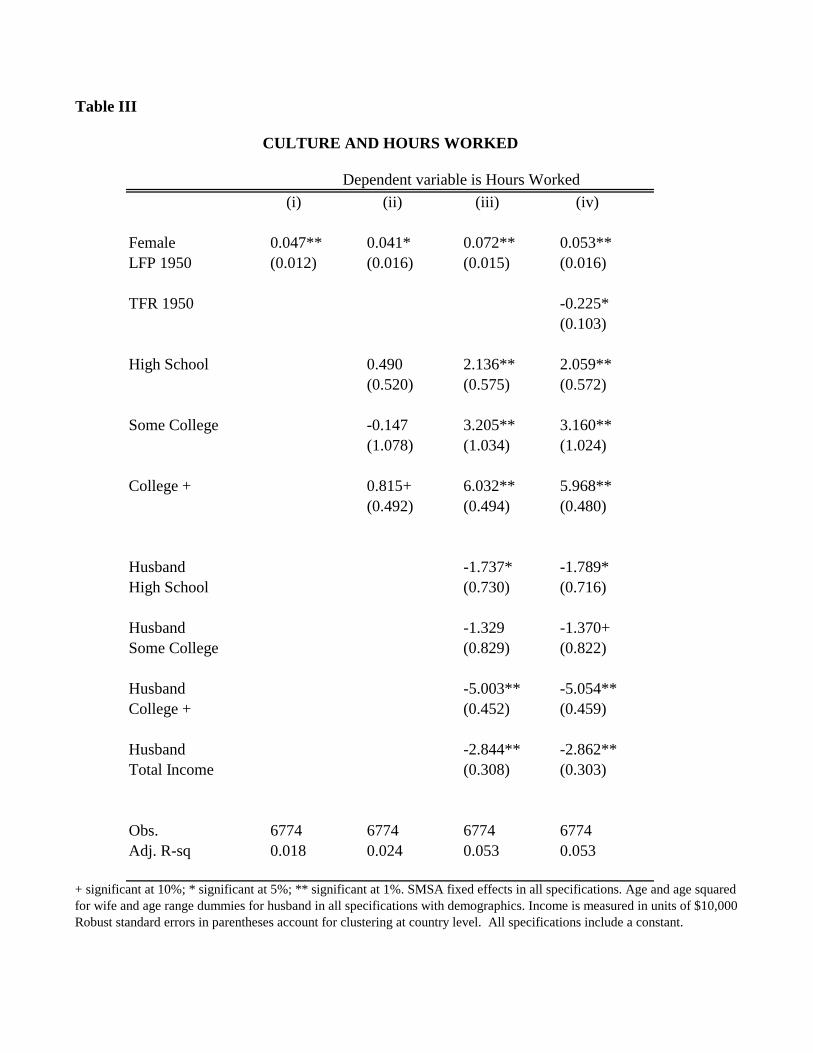
Table III

(i) (ii) (iii) (iv)

Female 0.047** 0.041* 0.072** 0.053**LFP 1950 (0.012) (0.016) (0.015) (0.016)

TFR 1950 -0.225*(0.103)

High School 0.490 2.136** 2.059**(0.520) (0.575) (0.572)

Some College -0.147 3.205** 3.160**(1.078) (1.034) (1.024)

College + 0.815+ 6.032** 5.968**(0.492) (0.494) (0.480)

Husband -1.737* -1.789*High School (0.730) (0.716)

Husband -1.329 -1.370+Some College (0.829) (0.822)

Husband -5.003** -5.054**College + (0.452) (0.459)

Husband -2.844** -2.862**Total Income (0.308) (0.303)

Obs. 6774 6774 6774 6774Adj. R-sq 0.018 0.024 0.053 0.053

+ significant at 10%; * significant at 5%; ** significant at 1%. SMSA fixed effects in all specifications. Age and age squaredfor wife and age range dummies for husband in all specifications with demographics. Income is measured in units of $10,000Robust standard errors in parentheses account for clustering at country level. All specifications include a constant.

Dependent variable is Hours Worked

CULTURE AND HOURS WORKED

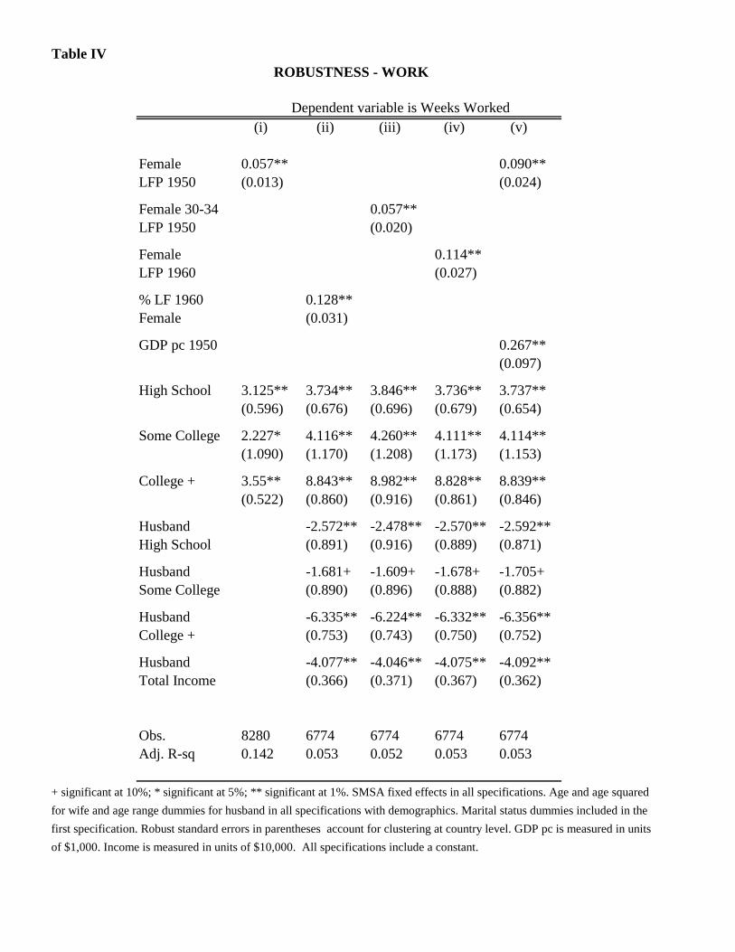
Table IV

(i) (ii) (iii) (iv) (v)

Female 0.057** 0.090**LFP 1950 (0.013) (0.024)

Female 30-34 0.057**LFP 1950 (0.020)

Female 0.114**LFP 1960 (0.027)

% LF 1960 0.128**Female (0.031)

GDP pc 1950 0.267**(0.097)

High School 3.125** 3.734** 3.846** 3.736** 3.737**(0.596) (0.676) (0.696) (0.679) (0.654)

Some College 2.227* 4.116** 4.260** 4.111** 4.114**(1.090) (1.170) (1.208) (1.173) (1.153)

College + 3.55** 8.843** 8.982** 8.828** 8.839**(0.522) (0.860) (0.916) (0.861) (0.846)

Husband -2.572** -2.478** -2.570** -2.592**High School (0.891) (0.916) (0.889) (0.871)

Husband -1.681+ -1.609+ -1.678+ -1.705+Some College (0.890) (0.896) (0.888) (0.882)

Husband -6.335** -6.224** -6.332** -6.356**College + (0.753) (0.743) (0.750) (0.752)

Husband -4.077** -4.046** -4.075** -4.092**Total Income (0.366) (0.371) (0.367) (0.362)

Obs. 8280 6774 6774 6774 6774Adj. R-sq 0.142 0.053 0.052 0.053 0.053


for wife and age range dummies for husband in all specifications with demographics. Marital status dummies included in the

first specification. Robust standard errors in parentheses account for clustering at country level. GDP pc is measured in units

of $1,000. Income is measured in units of $10,000. All specifications include a constant.

ROBUSTNESS - WORK

Dependent variable is Weeks Worked

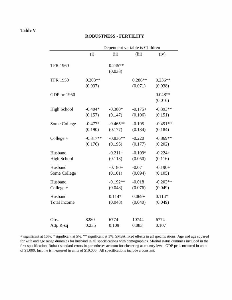
Table V

(i) (ii) (iii) (iv)

TFR 1960 0.245**(0.038)

TFR 1950 0.203** 0.286** 0.236**(0.037) (0.071) (0.038)

GDP pc 1950 0.048**(0.016)

High School -0.404* -0.380* -0.175+ -0.393**(0.157) (0.147) (0.106) (0.151)

Some College -0.477* -0.465** -0.195 -0.491**(0.190) (0.177) (0.134) (0.184)

College + -0.817** -0.836** -0.220 -0.869**(0.176) (0.195) (0.177) (0.202)

Husband -0.211+ -0.109* -0.224+High School (0.113) (0.050) (0.116)

Husband -0.180+ -0.071 -0.190+Some College (0.101) (0.094) (0.105)

Husband -0.192** -0.018 -0.202**College + (0.048) (0.076) (0.049)

Husband 0.114* 0.069+ 0.114*Total Income (0.048) (0.040) (0.049)

Obs. 8280 6774 10744 6774Adj. R-sq 0.235 0.109 0.083 0.107

+ significant at 10%; * significant at 5%; ** significant at 1%. SMSA fixed effects in all specifications. Age and age squaredfor wife and age range dummies for husband in all specifications with demographics. Marital status dummies included in thefirst specification. Robust standard errors in parentheses account for clustering at country level. GDP pc is meaured in unitsof $1,000. Income is measured in units of $10,000. All specifications include a constant.

ROBUSTNESS - FERTILITY

Dependent variable is Children

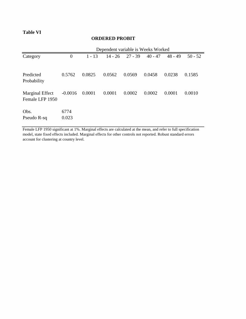
Table VI

Category 0 1 - 13 14 - 26 27 - 39 40 - 47 48 - 49 50 - 52

Predicted 0.5762 0.0825 0.0562 0.0569 0.0458 0.0238 0.1585Probability

Marginal Effect -0.0016 0.0001 0.0001 0.0002 0.0002 0.0001 0.0010Female LFP 1950

Obs. 6774Pseudo R-sq 0.023

Female LFP 1950 significant at 1%. Marginal effects are calculated at the mean, and refer to full specificationmodel, state fixed effects included. Marginal effects for other controls not reported. Robust standard errorsaccount for clustering at country level.


ORDERED PROBIT

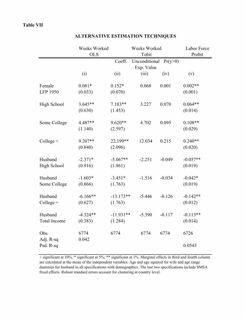
Weeks Worked Labor ForceOLS Probit

Coeff. Unconditional Pr(y>0)Exp. Value

(i) (ii) (iii) (iv) (v)

Female 0.081* 0.152* 0.068 0.001 0.002**LFP 1950 (0.033) (0.070) (0.001)

High School 3.645** 7.183** 3.227 0.070 0.064**(0.630) (1.453) (0.014)

Some College 4.487** 9.620** 4.702 0.095 0.108**(1.140) (2.597) (0.029)

College + 9.207** 22.199** 12.034 0.215 0.240**(0.840) (2.096) (0.020)

Husband -2.371* -5.067** -2.251 -0.049 -0.057**High School (0.916) (1.861) (0.019)

Husband -1.603* -3.451* -1.516 -0.034 -0.042*Some College (0.866) (1.763) (0.019)

Husband -6.166** -13.173** -5.446 -0.126 -0.142**College + (0.627) (1.763) (0.012)

Husband -4.324** -11.931** -5.390 -0.117 -0.113**Total Income (0.383) (1.284) (0.014)

Obs. 6774 6774 6774 6774 6726Adj. R-sq 0.042Psd. R-sq 0.0543

+ significant at 10%; * significant at 5%; ** significant at 1%. Marginal effects in third and fourth column are calculated at the mean of the independent variables. Age and age squared for wife and age rangedummies for husband in all specifications with demographics. The last two specifications include SMSAfixed effects. Robust standard errors account for clustering at country level.

Table VII

ALTERNATIVE ESTIMATION TECHNIQUES

Weeks WorkedTobit

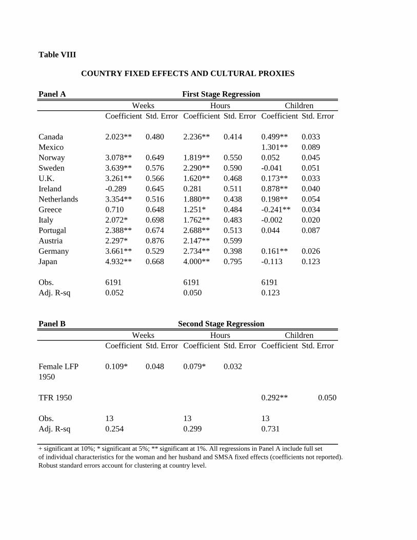
Table VIII

Panel A

Coefficient Std. Error Coefficient Std. Error Coefficient Std. Error

Canada 2.023** 0.480 2.236** 0.414 0.499** 0.033Mexico 1.301** 0.089Norway 3.078** 0.649 1.819** 0.550 0.052 0.045Sweden 3.639** 0.576 2.290** 0.590 -0.041 0.051U.K. 3.261** 0.566 1.620** 0.468 0.173** 0.033Ireland -0.289 0.645 0.281 0.511 0.878** 0.040Netherlands 3.354** 0.516 1.880** 0.438 0.198** 0.054Greece 0.710 0.648 1.251* 0.484 -0.241** 0.034Italy 2.072* 0.698 1.762** 0.483 -0.002 0.020Portugal 2.388** 0.674 2.688** 0.513 0.044 0.087Austria 2.297* 0.876 2.147** 0.599Germany 3.661** 0.529 2.734** 0.398 0.161** 0.026Japan 4.932** 0.668 4.000** 0.795 -0.113 0.123

Obs. 6191 6191 6191Adj. R-sq 0.052 0.050 0.123

Panel B

Coefficient Std. Error Coefficient Std. Error Coefficient Std. Error

Female LFP 0.109* 0.048 0.079* 0.0321950

TFR 1950 0.292** 0.050

Obs. 13 13 13Adj. R-sq 0.254 0.299 0.731

+ significant at 10%; * significant at 5%; ** significant at 1%. All regressions in Panel A include full setof individual characteristics for the woman and her husband and SMSA fixed effects (coefficients not reported).Robust standard errors account for clustering at country level.

Weeks Hours Children

COUNTRY FIXED EFFECTS AND CULTURAL PROXIES

First Stage Regression

Second Stage RegressionWeeks Hours Children

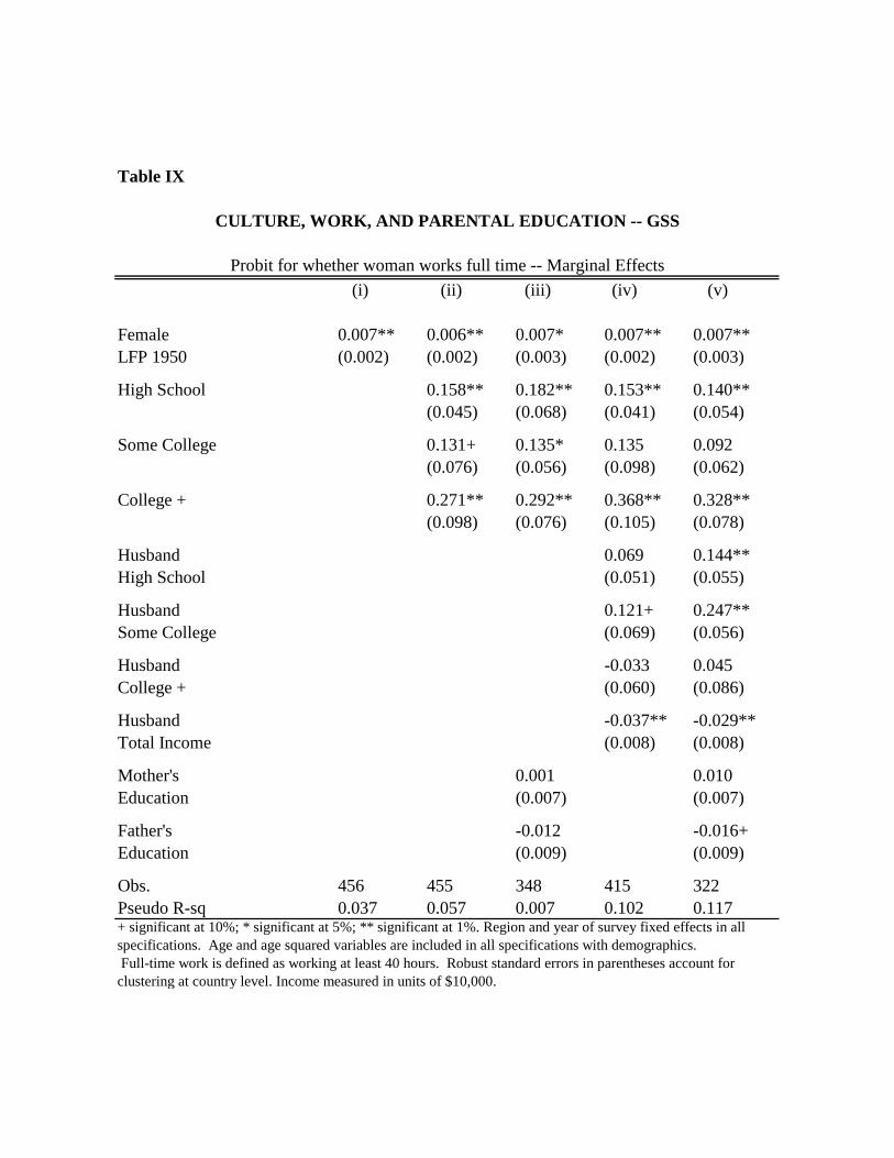
Table IX

(i) (ii) (iii) (iv) (v)

Female 0.007** 0.006** 0.007* 0.007** 0.007**LFP 1950 (0.002) (0.002) (0.003) (0.002) (0.003)

High School 0.158** 0.182** 0.153** 0.140**(0.045) (0.068) (0.041) (0.054)

Some College 0.131+ 0.135* 0.135 0.092(0.076) (0.056) (0.098) (0.062)

College + 0.271** 0.292** 0.368** 0.328**(0.098) (0.076) (0.105) (0.078)

Husband 0.069 0.144**High School (0.051) (0.055)

Husband 0.121+ 0.247**Some College (0.069) (0.056)

Husband -0.033 0.045College + (0.060) (0.086)


Mother's 0.001 0.010Education (0.007) (0.007)

Father's -0.012 -0.016+Education (0.009) (0.009)

Obs. 456 455 348 415 322Pseudo R-sq 0.037 0.057 0.007 0.102 0.117+ significant at 10%; * significant at 5%; ** significant at 1%. Region and year of survey fixed effects in allspecifications. Age and age squared variables are included in all specifications with demographics.Full-time work is defined as working at least 40 hours. Robust standard errors in parentheses account for

clustering at country level. Income measured in units of $10,000.

CULTURE, WORK, AND PARENTAL EDUCATION -- GSS

Probit for whether woman works full time -- Marginal Effects

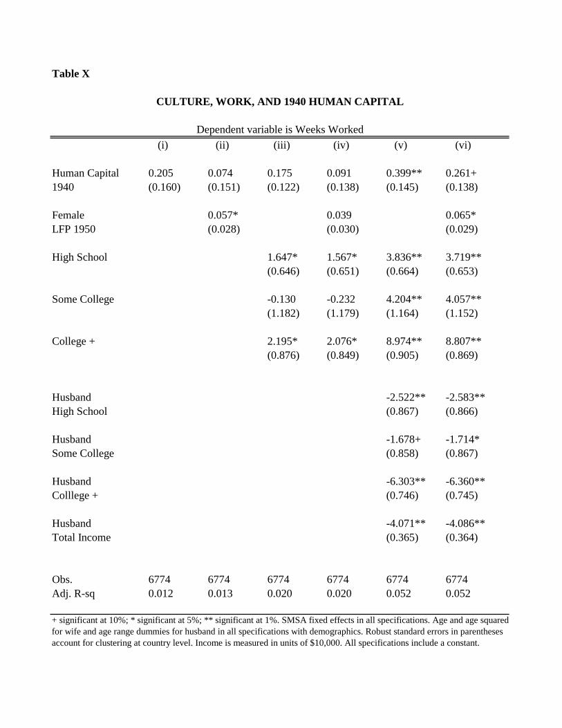
Table X

(i) (ii) (iii) (iv) (v) (vi)

Human Capital 0.205 0.074 0.175 0.091 0.399** 0.261+1940 (0.160) (0.151) (0.122) (0.138) (0.145) (0.138)

Female 0.057* 0.039 0.065*LFP 1950 (0.028) (0.030) (0.029)

High School 1.647* 1.567* 3.836** 3.719**(0.646) (0.651) (0.664) (0.653)

Some College -0.130 -0.232 4.204** 4.057**(1.182) (1.179) (1.164) (1.152)

College + 2.195* 2.076* 8.974** 8.807**(0.876) (0.849) (0.905) (0.869)

Husband -2.522** -2.583**High School (0.867) (0.866)

Husband -1.678+ -1.714*Some College (0.858) (0.867)

Husband -6.303** -6.360**Colllege + (0.746) (0.745)


Obs. 6774 6774 6774 6774 6774 6774Adj. R-sq 0.012 0.013 0.020 0.020 0.052 0.052

+ significant at 10%; * significant at 5%; ** significant at 1%. SMSA fixed effects in all specifications. Age and age squaredfor wife and age range dummies for husband in all specifications with demographics. Robust standard errors in parenthesesaccount for clustering at country level. Income is measured in units of $10,000. All specifications include a constant.

CULTURE, WORK, AND 1940 HUMAN CAPITAL


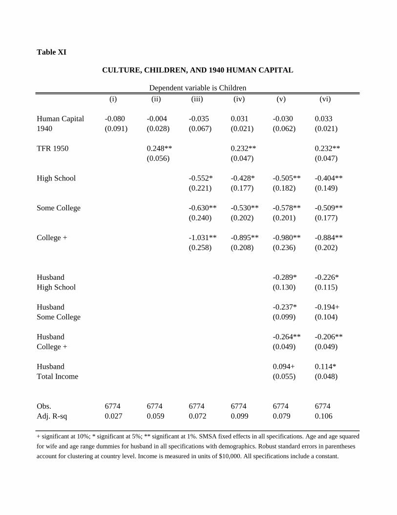
Table XI

(i) (ii) (iii) (iv) (v) (vi)

Human Capital -0.080 -0.004 -0.035 0.031 -0.030 0.0331940 (0.091) (0.028) (0.067) (0.021) (0.062) (0.021)

TFR 1950 0.248** 0.232** 0.232**(0.056) (0.047) (0.047)

High School -0.552* -0.428* -0.505** -0.404**(0.221) (0.177) (0.182) (0.149)

Some College -0.630** -0.530** -0.578** -0.509**(0.240) (0.202) (0.201) (0.177)

College + -1.031** -0.895** -0.980** -0.884**(0.258) (0.208) (0.236) (0.202)


Husband -0.237* -0.194+Some College (0.099) (0.104)

Husband -0.264** -0.206**College + (0.049) (0.049)

Husband 0.094+ 0.114*Total Income (0.055) (0.048)

Obs. 6774 6774 6774 6774 6774 6774Adj. R-sq 0.027 0.059 0.072 0.099 0.079 0.106




CULTURE, CHILDREN, AND 1940 HUMAN CAPITAL


Table XII

(i) (ii) (iii) (iv) (v) (vi)

Human Capital 0.153 -0.224 0.075 -0.292 0.486** 0.1551970 (0.155) (0.234) (0.134) (0.203) (0.136) (0.209)

Female 0.067** 0.065* 0.059*LFP 1950 (0.023) (0.025) (0.026)

High School 0.590* 0.592 2.096** 2.093**(0.491) (0.493) (0.546) (0.547)

Some College 0.000 -0.012 3.169** 3.151**(1.060) (1.060) (1.002) (1.004)

College + 0.973+ 0.969+ 5.985** 5.973**(0.537) (0.528) (0.498) (0.482)


Husband -1.374 -1.358Some College (0.819) (0.826)

Husband -5.044** -5.036**Colllege + (0.471) (0.465)


Obs. 6774 6774 6774 6774 6774 6774Adj. R-sq 0.017 0.018 0.023 0.024 0.052 0.053


CULTURE, WORK, AND 1970 HUMAN CAPITAL


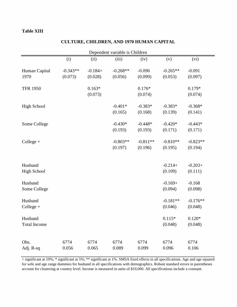
Table XIII

(i) (ii) (iii) (iv) (v) (vi)

Human Capital -0.343** -0.184+ -0.268** -0.096 -0.265** -0.0911970 (0.073) (0.028) (0.056) (0.099) (0.053) (0.097)

TFR 1950 0.163* 0.176* 0.179*(0.073) (0.074) (0.074)

High School -0.401* -0.383* -0.383* -0.368*(0.165) (0.168) (0.139) (0.141)

Some College -0.430* -0.448* -0.420* -0.443*(0.193) (0.193) (0.171) (0.171)

College + -0.803** -0.811** -0.810** -0.823**(0.197) (0.196) (0.195) (0.194)

Husband -0.214+ -0.203+High School (0.109) (0.111)

Husband -0.169+ -0.168Some College (0.094) (0.098)

Husband -0.181** -0.176**College + (0.046) (0.048)

Husband 0.115* 0.120*Total Income (0.048) (0.048)

Obs. 6774 6774 6774 6774 6774 6774Adj. R-sq 0.056 0.065 0.089 0.099 0.096 0.106


CULTURE, CHILDREN, AND 1970 HUMAN CAPITAL


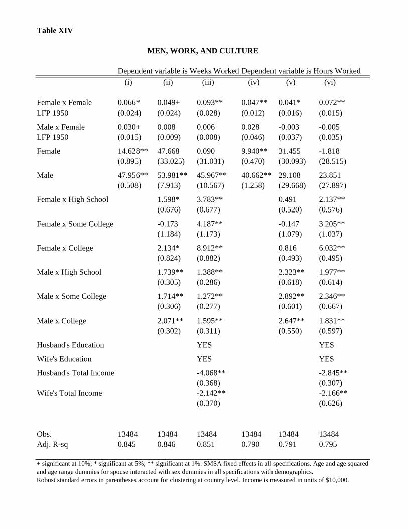
Table XIV

Dependent variable is Weeks Worked Dependent variable is Hours Worked

(i) (ii) (iii) (iv) (v) (vi)

Female x Female 0.066* 0.049+ 0.093** 0.047** 0.041* 0.072**LFP 1950 (0.024) (0.024) (0.028) (0.012) (0.016) (0.015)

Male x Female 0.030+ 0.008 0.006 0.028 -0.003 -0.005LFP 1950 (0.015) (0.009) (0.008) (0.046) (0.037) (0.035)

Female 14.628** 47.668 0.090 9.940** 31.455 -1.818(0.895) (33.025) (31.031) (0.470) (30.093) (28.515)

Male 47.956** 53.981** 45.967** 40.662** 29.108 23.851(0.508) (7.913) (10.567) (1.258) (29.668) (27.897)

Female x High School 1.598* 3.783** 0.491 2.137**(0.676) (0.677) (0.520) (0.576)

Female x Some College -0.173 4.187** -0.147 3.205**(1.184) (1.173) (1.079) (1.037)

Female x College 2.134* 8.912** 0.816 6.032**(0.824) (0.882) (0.493) (0.495)

Male x High School 1.739** 1.388** 2.323** 1.977**(0.305) (0.286) (0.618) (0.614)

Male x Some College 1.714** 1.272** 2.892** 2.346**(0.306) (0.277) (0.601) (0.667)

Male x College 2.071** 1.595** 2.647** 1.831**(0.302) (0.311) (0.550) (0.597)

Husband's Education YES YES

Wife's Education YES YES

Husband's Total Income -4.068** -2.845**(0.368) (0.307)

Wife's Total Income -2.142** -2.166**(0.370) (0.626)

Obs. 13484 13484 13484 13484 13484 13484Adj. R-sq 0.845 0.846 0.851 0.790 0.791 0.795

+ significant at 10%; * significant at 5%; ** significant at 1%. SMSA fixed effects in all specifications. Age and age squaredand age range dummies for spouse interacted with sex dummies in all specifications with demographics.Robust standard errors in parentheses account for clustering at country level. Income is measured in units of $10,000.

MEN, WORK, AND CULTURE

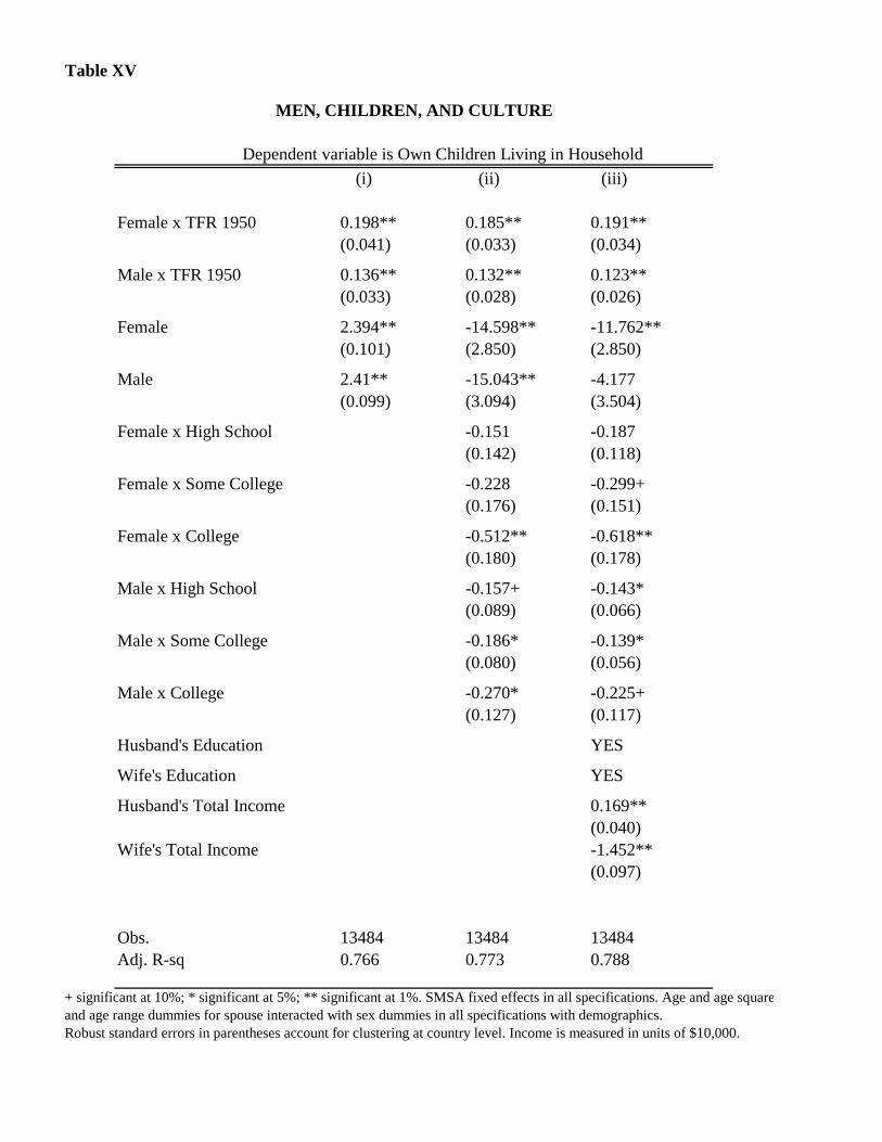
Table XV

Dependent variable is Own Children Living in Household

(i) (ii) (iii)

Female x TFR 1950 0.198** 0.185** 0.191**(0.041) (0.033) (0.034)

Male x TFR 1950 0.136** 0.132** 0.123**(0.033) (0.028) (0.026)

Female 2.394** -14.598** -11.762**(0.101) (2.850) (2.850)

Male 2.41** -15.043** -4.177(0.099) (3.094) (3.504)

Female x High School -0.151 -0.187(0.142) (0.118)

Female x Some College -0.228 -0.299+(0.176) (0.151)

Female x College -0.512** -0.618**(0.180) (0.178)

Male x High School -0.157+ -0.143*(0.089) (0.066)

Male x Some College -0.186* -0.139*(0.080) (0.056)

Male x College -0.270* -0.225+(0.127) (0.117)

Husband's Education YES

Wife's Education YES

Husband's Total Income 0.169**(0.040)

Wife's Total Income -1.452**(0.097)

Obs. 13484 13484 13484Adj. R-sq 0.766 0.773 0.788

+ significant at 10%; * significant at 5%; ** significant at 1%. SMSA fixed effects in all specifications. Age and age squaredand age range dummies for spouse interacted with sex dummies in all specifications with demographics.Robust standard errors in parentheses account for clustering at country level. Income is measured in units of $10,000.

MEN, CHILDREN, AND CULTURE

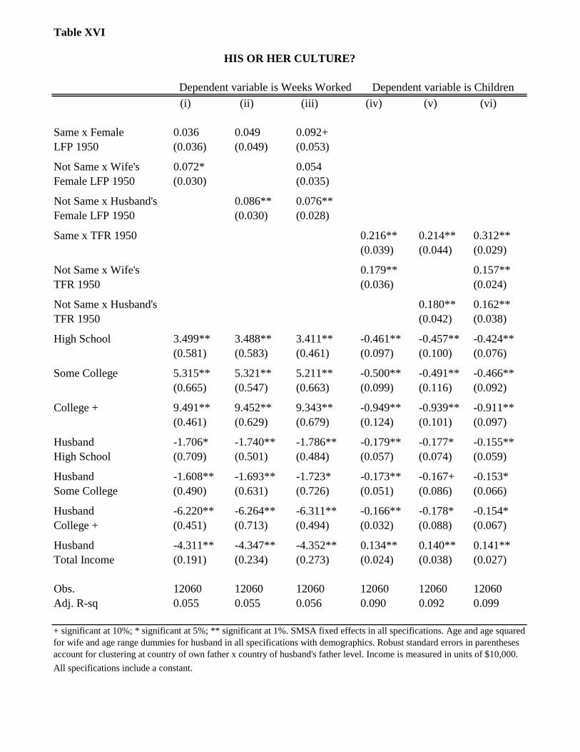
Table XVI

(i) (ii) (iii) (iv) (v) (vi)

Same x Female 0.036 0.049 0.092+LFP 1950 (0.036) (0.049) (0.053)

Not Same x Wife's 0.072* 0.054Female LFP 1950 (0.030) (0.035)

Not Same x Husband's 0.086** 0.076**Female LFP 1950 (0.030) (0.028)

Same x TFR 1950 0.216** 0.214** 0.312**(0.039) (0.044) (0.029)

Not Same x Wife's 0.179** 0.157**TFR 1950 (0.036) (0.024)

Not Same x Husband's 0.180** 0.162**TFR 1950 (0.042) (0.038)

High School 3.499** 3.488** 3.411** -0.461** -0.457** -0.424**(0.581) (0.583) (0.461) (0.097) (0.100) (0.076)

Some College 5.315** 5.321** 5.211** -0.500** -0.491** -0.466**(0.665) (0.547) (0.663) (0.099) (0.116) (0.092)

College + 9.491** 9.452** 9.343** -0.949** -0.939** -0.911**(0.461) (0.629) (0.679) (0.124) (0.101) (0.097)

Husband -1.706* -1.740** -1.786** -0.179** -0.177* -0.155**High School (0.709) (0.501) (0.484) (0.057) (0.074) (0.059)

Husband -1.608** -1.693** -1.723* -0.173** -0.167+ -0.153*Some College (0.490) (0.631) (0.726) (0.051) (0.086) (0.066)

Husband -6.220** -6.264** -6.311** -0.166** -0.178* -0.154*College + (0.451) (0.713) (0.494) (0.032) (0.088) (0.067)

Husband -4.311** -4.347** -4.352** 0.134** 0.140** 0.141**Total Income (0.191) (0.234) (0.273) (0.024) (0.038) (0.027)

Obs. 12060 12060 12060 12060 12060 12060Adj. R-sq 0.055 0.055 0.056 0.090 0.092 0.099

+ significant at 10%; * significant at 5%; ** significant at 1%. SMSA fixed effects in all specifications. Age and age squaredfor wife and age range dummies for husband in all specifications with demographics. Robust standard errors in parenthesesaccount for clustering at country of own father x country of husband's father level. Income is measured in units of $10,000.

All specifications include a constant.

HIS OR HER CULTURE?

Dependent variable is Weeks Worked Dependent variable is Children

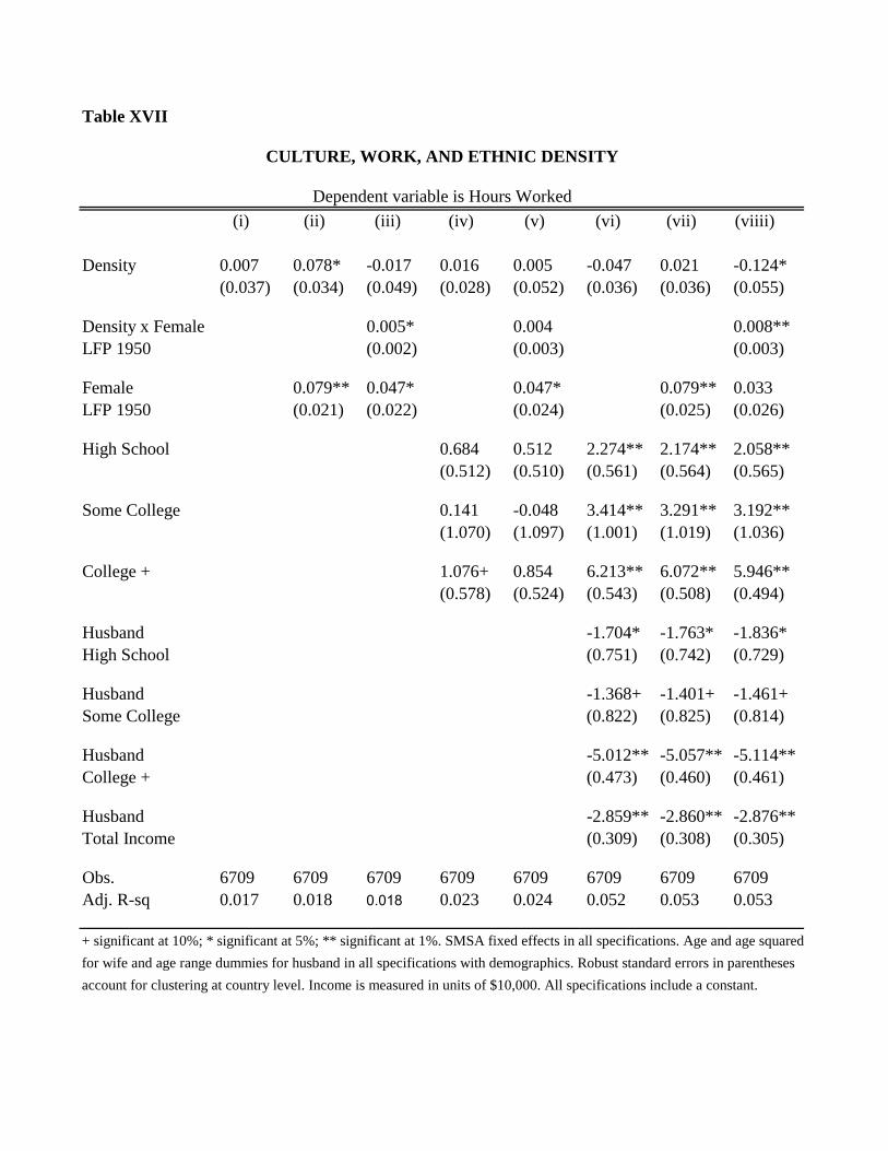
Table XVII

(i) (ii) (iii) (iv) (v) (vi) (vii) (viiii)

Density 0.007 0.078* -0.017 0.016 0.005 -0.047 0.021 -0.124*(0.037) (0.034) (0.049) (0.028) (0.052) (0.036) (0.036) (0.055)

Density x Female 0.005* 0.004 0.008**LFP 1950 (0.002) (0.003) (0.003)

Female 0.079** 0.047* 0.047* 0.079** 0.033LFP 1950 (0.021) (0.022) (0.024) (0.025) (0.026)

High School 0.684 0.512 2.274** 2.174** 2.058**(0.512) (0.510) (0.561) (0.564) (0.565)

Some College 0.141 -0.048 3.414** 3.291** 3.192**(1.070) (1.097) (1.001) (1.019) (1.036)

College + 1.076+ 0.854 6.213** 6.072** 5.946**(0.578) (0.524) (0.543) (0.508) (0.494)

Husband -1.704* -1.763* -1.836*High School (0.751) (0.742) (0.729)

Husband -1.368+ -1.401+ -1.461+Some College (0.822) (0.825) (0.814)

Husband -5.012** -5.057** -5.114**College + (0.473) (0.460) (0.461)

Husband -2.859** -2.860** -2.876**Total Income (0.309) (0.308) (0.305)

Obs. 6709 6709 6709 6709 6709 6709 6709 6709Adj. R-sq 0.017 0.018 0.018 0.023 0.024 0.052 0.053 0.053




CULTURE, WORK, AND ETHNIC DENSITY


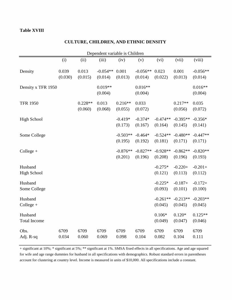
Table XVIII

(i) (ii) (iii) (iv) (v) (vi) (vii) (viii)

Density 0.039 0.013 -0.054** 0.001 -0.056** 0.023 0.001 -0.056**(0.030) (0.015) (0.014) (0.013) (0.014) (0.022) (0.013) (0.014)

Density x TFR 1950 0.019** 0.016** 0.016**(0.004) (0.004) (0.004)

TFR 1950 0.228** 0.013 0.216** 0.033 0.217** 0.035(0.060) (0.068) (0.055) (0.072) (0.056) (0.072)

High School -0.419* -0.374* -0.474** -0.395** -0.356*(0.173) (0.167) (0.164) (0.145) (0.141)

Some College -0.503** -0.464* -0.524** -0.480** -0.447**(0.195) (0.192) (0.181) (0.171) (0.171)

College + -0.876** -0.827** -0.928** -0.862** -0.820**(0.201) (0.196) (0.208) (0.196) (0.193)

Husband -0.275* -0.220+ -0.201+High School (0.121) (0.113) (0.112)

Husband -0.225* -0.187+ -0.172+Some College (0.093) (0.101) (0.100)

Husband -0.261** -0.213** -0.203**College + (0.045) (0.045) (0.045)

Husband 0.106* 0.120* 0.125**Total Income (0.049) (0.047) (0.046)

Obs. 6709 6709 6709 6709 6709 6709 6709 6709Adj. R-sq 0.034 0.060 0.069 0.098 0.104 0.082 0.104 0.111




CULTURE, CHILDREN, AND ETHNIC DENSITY


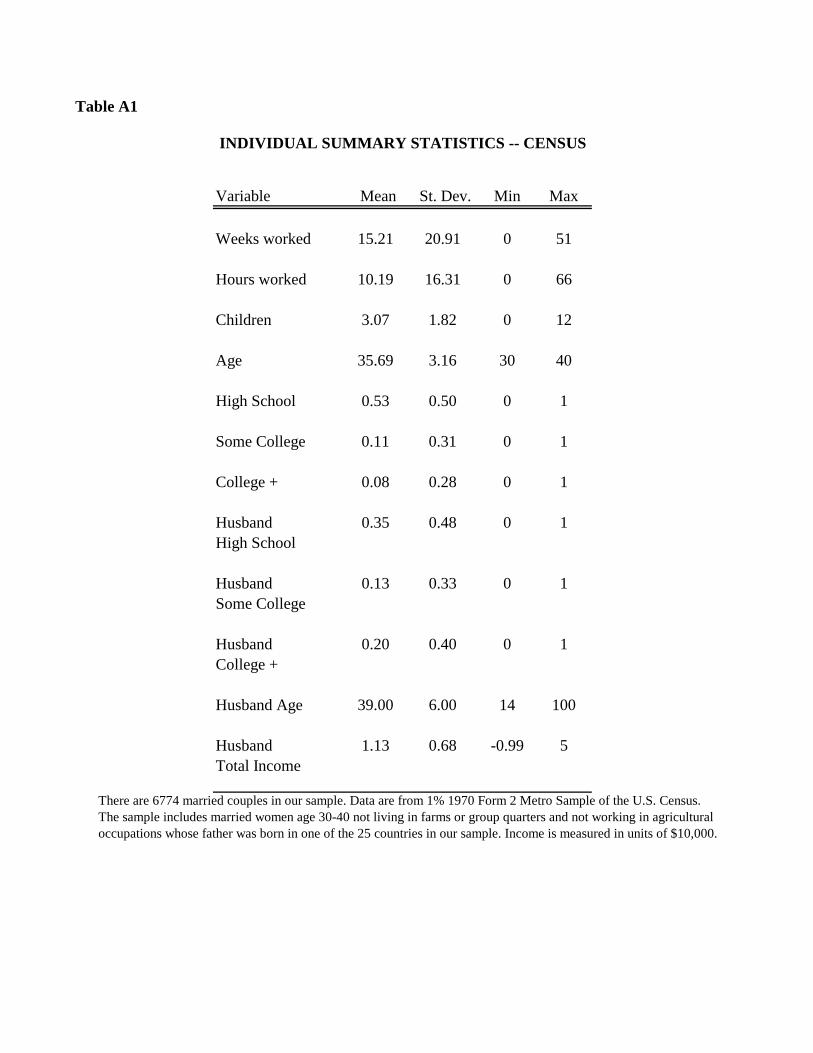
Table A1

Variable Mean St. Dev. Min Max

Weeks worked 15.21 20.91 0 51

Hours worked 10.19 16.31 0 66

Children 3.07 1.82 0 12

Age 35.69 3.16 30 40

High School 0.53 0.50 0 1

Some College 0.11 0.31 0 1

College + 0.08 0.28 0 1

Husband 0.35 0.48 0 1High School

Husband 0.13 0.33 0 1Some College

Husband 0.20 0.40 0 1College +

Husband Age 39.00 6.00 14 100

Husband 1.13 0.68 -0.99 5Total Income

The sample includes married women age 30-40 not living in farms or group quarters and not working in agricultural

INDIVIDUAL SUMMARY STATISTICS -- CENSUS

There are 6774 married couples in our sample. Data are from 1% 1970 Form 2 Metro Sample of the U.S. Census.

occupations whose father was born in one of the 25 countries in our sample. Income is measured in units of $10,000.

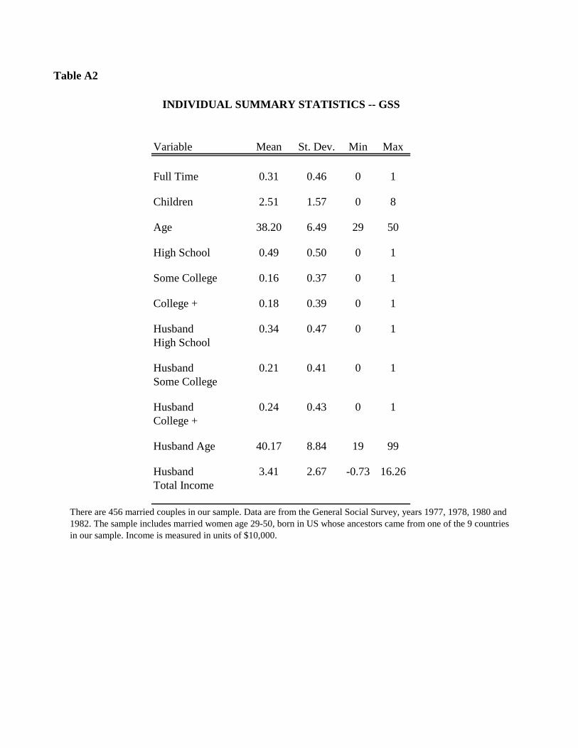
Table A2

Variable Mean St. Dev. Min Max

Full Time 0.31 0.46 0 1

Children 2.51 1.57 0 8

Age 38.20 6.49 29 50

High School 0.49 0.50 0 1

Some College 0.16 0.37 0 1

College + 0.18 0.39 0 1

Husband 0.34 0.47 0 1High School

Husband 0.21 0.41 0 1Some College

Husband 0.24 0.43 0 1College +

Husband Age 40.17 8.84 19 99

Husband 3.41 2.67 -0.73 16.26Total Income

1982. The sample includes married women age 29-50, born in US whose ancestors came from one of the 9 countriesin our sample. Income is measured in units of $10,000.

There are 456 married couples in our sample. Data are from the General Social Survey, years 1977, 1978, 1980 and

INDIVIDUAL SUMMARY STATISTICS -- GSS

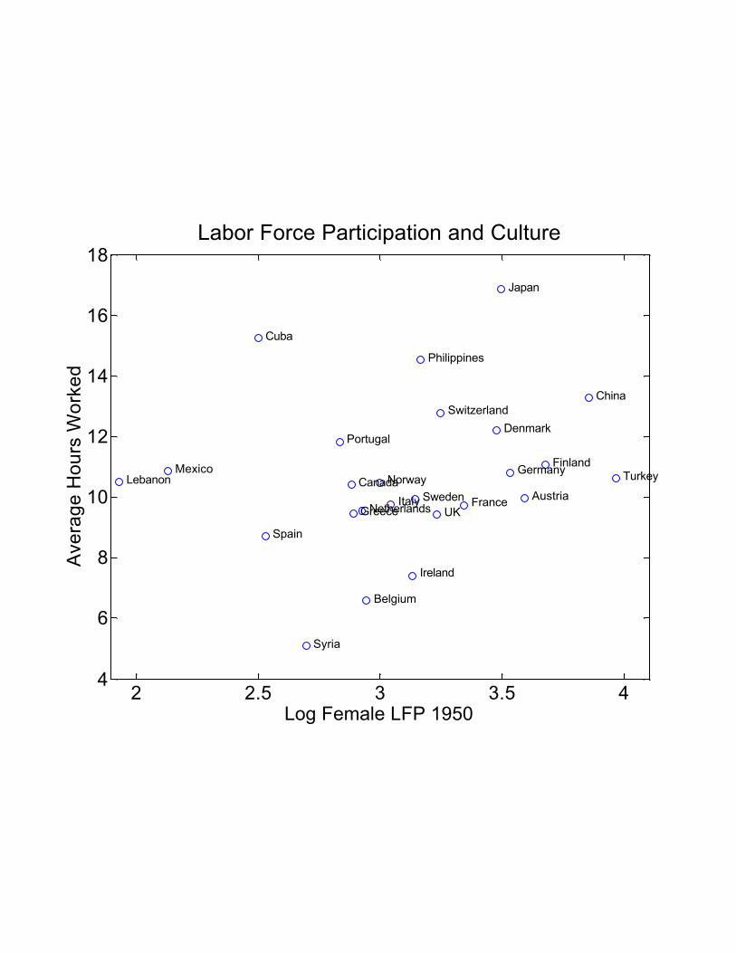
2 2.5 3 3.5 44

6

8

10

12

14

16

18

Canada Mexico

Cuba

Denmark

Finland Norway

Sweden UK

Ireland

Belgium

France Netherlands

Switzerland

Greece Italy

Portugal

Spain

Austria

Germany

China

Japan

Philippines

Lebanon

Syria

Turkey

Log Female LFP 1950

Aver

age

Hou

rs W

orke

d

Labor Force Participation and Culture

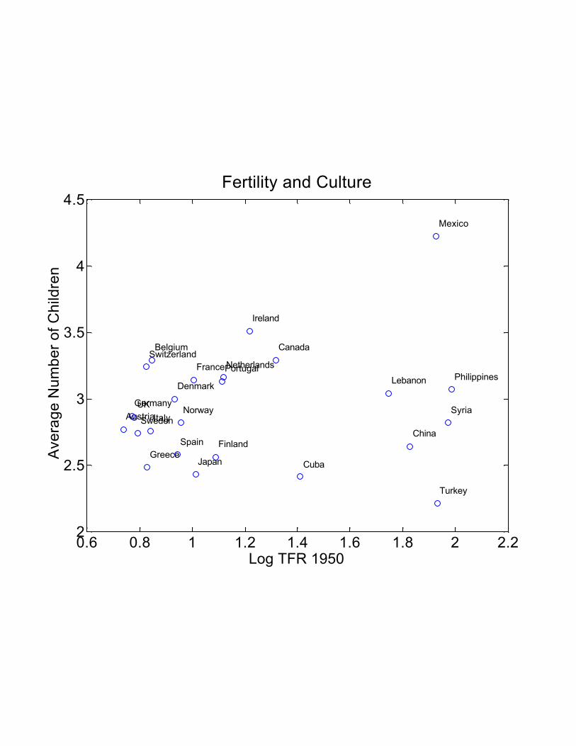
0.6 0.8 1 1.2 1.4 1.6 1.8 2 2.22

2.5

3

3.5

4

4.5

Canada

Mexico

Cuba

Denmark

Finland

Norway Sweden

UK

Ireland

Belgium

France NetherlandsSwitzerland

Greece

Italy

Portugal

Spain

Austria Germany

China

Japan

PhilippinesLebanon

Syria

Turkey

Log TFR 1950

Aver

age

Num

ber o

f Chi

ldre

n

Fertility and Culture

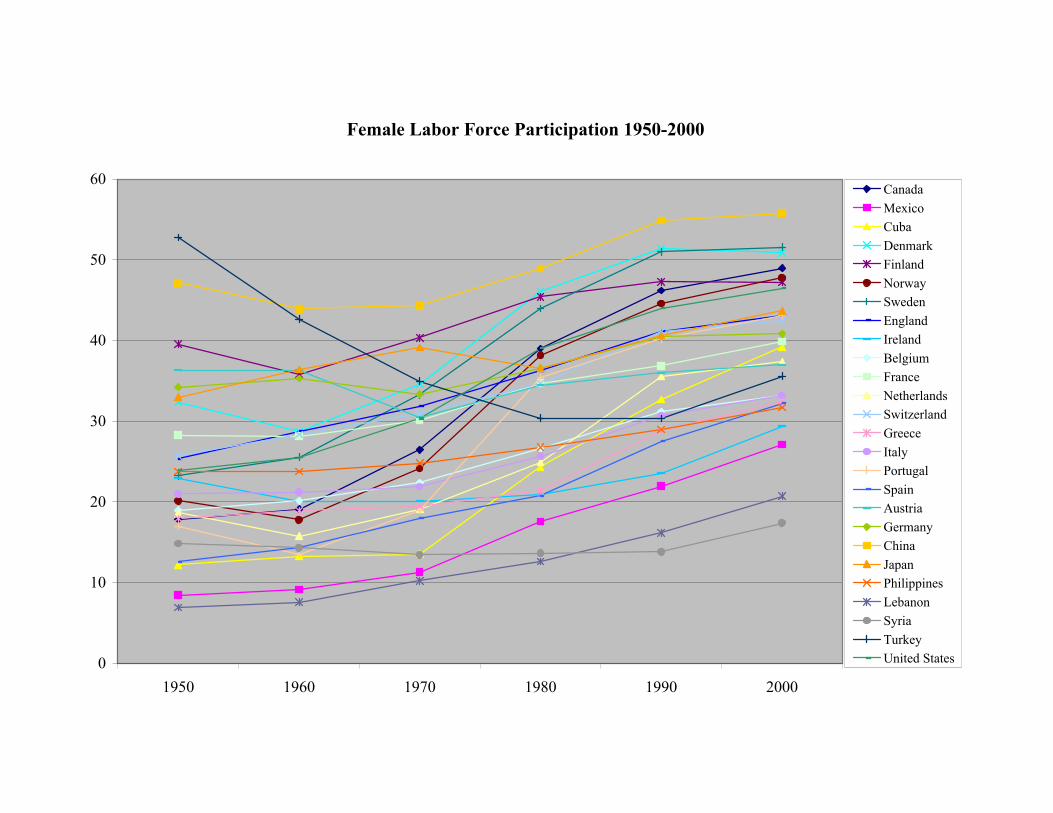
Female Labor Force Participation 1950-2000

0

10

20

30

40

50

60

1950 1960 1970 1980 1990 2000

CanadaMexicoCubaDenmarkFinlandNorwaySwedenEnglandIrelandBelgiumFranceNetherlandsSwitzerlandGreeceItalyPortugalSpainAustriaGermanyChinaJapanPhilippinesLebanonSyriaTurkeyUnited States

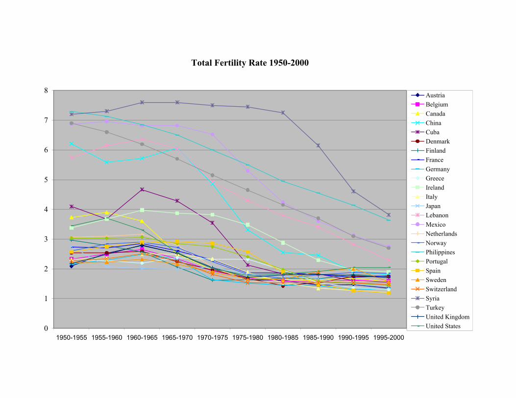
Total Fertility Rate 1950-2000

0

1

2

3

4

5

6

7

8

1950-1955 1955-1960 1960-1965 1965-1970 1970-1975 1975-1980 1980-1985 1985-1990 1990-1995 1995-2000

AustriaBelgiumCanadaChinaCubaDenmarkFinlandFranceGermanyGreeceIrelandItalyJapanLebanonMexicoNetherlandsNorwayPhilippinesPortugalSpainSwedenSwitzerlandSyriaTurkeyUnited KingdomUnited States

Culture: An Empirical Investigation of Beliefs, Work, and Fertility

Documents