Development Economics Slides 5 Debraj Ray Columbia, Fall 2013 Transitions between one equilibrium and another An empirical example Fertility transition in Bangladesh (Munshi-Myaux 2006 JDE) Population: Quick Background Population Landmark Date Achieved Years Taken 1 billion 1804 1 2 billion 1927 123 3 billion 1960 33 4 billion 1974 14 5 billion 1987 13 6 billion 1998 11 7 billion 2011 13 Population growth ) economic development Solow, technical progress Economic development ) population growth demographic transition (phrase hides a lot of detail)

Welcome message from author
This document is posted to help you gain knowledge. Please leave a comment to let me know what you think about it! Share it to your friends and learn new things together.
Transcript

Development Economics
Slides 5
Debraj Ray
Columbia, Fall 2013
Transitions between one equilibrium and another
An empirical example
Fertility transition in Bangladesh (Munshi-Myaux 2006 JDE)
0-0
Population: Quick Background
Population Landmark Date Achieved Years Taken
1 billion 1804 12 billion 1927 1233 billion 1960 334 billion 1974 145 billion 1987 136 billion 1998 117 billion 2011 13
Population growth ) economic development
Solow, technical progress
Economic development ) population growth
demographic transition (phrase hides a lot of detail)
0-1

Geographical Distribution of Population
1650 1750 1800 1850 1900 1960 2008
World pop (m) 545 728 906 1,171 1,608 3,023 6,750
PercentagesEurope 18.3 19.2 20.7 22.7 24.9 20.0 10.8N. America 0.2 0.1 0.7 2.3 5.1 6.8 5.1Oceania 0.4 0.3 0.2 0.2 0.4 0.5 0.5L. America 2.2 1.5 2.1 2.8 3.9 7.3 8.5Africa 18.3 13.1 9.9 8.1 7.4 9.4 14.6Asia 60.6 65.8 66.4 63.9 58.3 56.0 60.4
0-2
Birth and Death Rates (Per Thousand), 1995
Country pc income Birth rate Death rate Pop growth
I.Mali 520 51 20 3.1Malawi 690 51 20 3.1Sierra Leone 750 49 25 2.4Guinea-Bissau 840 43 21 2.2II.Kenya 1,290 45 12 3.3Nigeria 1,400 45 15 3.0Ghana 1,970 42 12 3.0Pakistan 2,170 41 9 3.2III.India 1,220 29 10 1.9Bangladesh 1,290 36 12 2.4
0-3
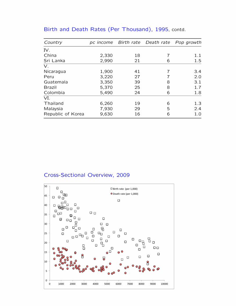
Birth and Death Rates (Per Thousand), 1995, contd.
Country pc income Birth rate Death rate Pop growth
IV.China 2,330 18 7 1.1Sri Lanka 2,990 21 6 1.5V.Nicaragua 1,900 41 7 3.4Peru 3,220 27 7 2.0Guatemala 3,350 39 8 3.1Brazil 5,370 25 8 1.7Colombia 5,490 24 6 1.8VI.Thailand 6,260 19 6 1.3Malaysia 7,930 29 5 2.4Republic of Korea 9,630 16 6 1.0
0-4
Cross-Sectional Overview, 2009
0"
5"
10"
15"
20"
25"
30"
35"
40"
45"
50"
0" 1000" 2000" 3000" 4000" 5000" 6000" 7000" 8000" 9000" 10000"
Birth"rate""(per"1,000)"
Death"rate"(per"1,000)"
0-5
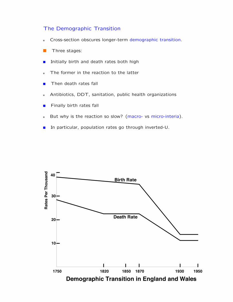
The Demographic Transition
Cross-section obscures longer-term demographic transition.
Three stages:
Initially birth and death rates both high
The former in the reaction to the latter
Then death rates fall
Antibiotics, DDT, sanitation, public health organizations
Finally birth rates fall
But why is the reaction so slow? (macro- vs micro-interia).
In particular, population rates go through inverted-U.
0-6
40
30
20
10
1750 1820 1850 1870 1930 1950
Demographic Transition in England and Wales
Birth Rate
Death Rate
Rate
s Pe
r Tho
usan
d
40
30
20
10
Demographic Transition in Sri Lanka1915 19921925 1937 1950 1955 1965 1975 1980 1985
Birth Rate
Death Rate
Rate
s Pe
r Tho
usan
d
0-7

40
30
20
10
1750 1820 1850 1870 1930 1950
Demographic Transition in England and Wales
Birth Rate
Death Rate
Rat
es P
er T
hous
and
40
30
20
10
Demographic Transition in Sri Lanka1915 19921925 1937 1950 1955 1965 1975 1980 1985
Birth Rate
Death Rate
Rat
es P
er T
hous
and
0-8
Demographic Transition, Sweden
0-9
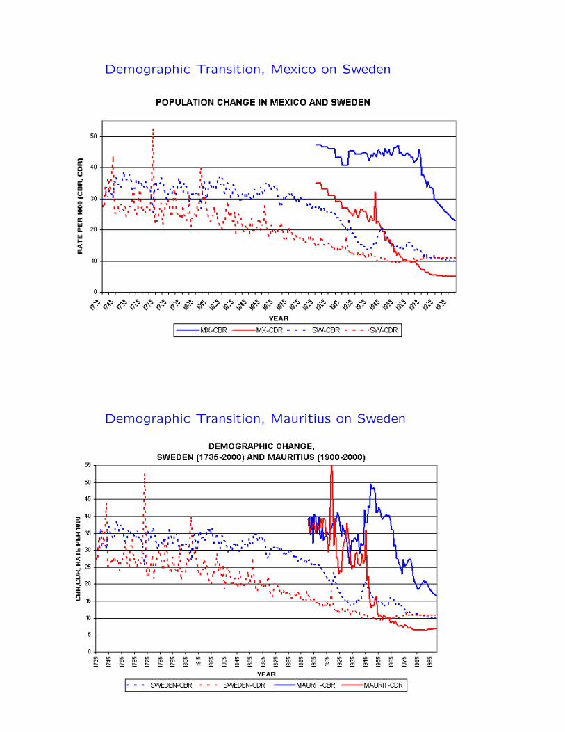
Demographic Transition, Mexico on Sweden
0-10
Demographic Transition, Mauritius on Sweden
0-11

Part of the reason for high birth rates is macro-inertia:
!"
#!"
$!"
%!"
&!"
'!"
(!"
)!"
*!"
+!"
#!!"
%$)"
)('"
+'!"
#!*&"
##('"
#&'!"
#')+"
$!#+"
$$*'"
$''("
$+&#"
%(*)"
&!&+"
&'$%"
&)%%"
'&&&"
(%!&"
)'+("
*#)%"
*)#("
#!$%)"
##&()"
#$+*("
#%)!("
#&$'*"
#)!'+"
$!!%)"
$'!'*"
$)#%%"
%!)$*"
%&)*)"
%()%%"
%**!&"
&'#&!"
(!(%%"
(',"
#'-(&"
"!-#&"
0-12
And micro-inertia has two broad sources:
“Demand” for children (child labor, old-age security)
“Supply” of children (opportunity cost of having them)
0-13
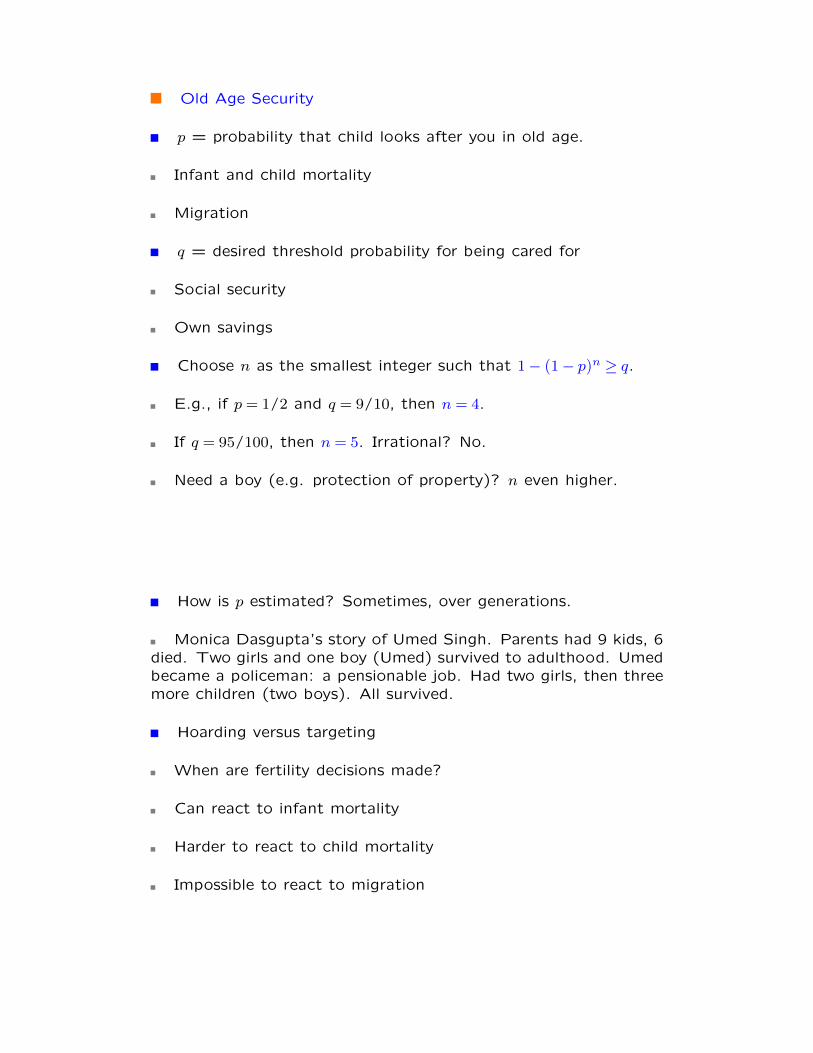
Old Age Security
p = probability that child looks after you in old age.
Infant and child mortality
Migration
q = desired threshold probability for being cared for
Social security
Own savings
Choose n as the smallest integer such that 1� (1� p)n � q.
E.g., if p = 1/2 and q = 9/10, then n = 4.
If q = 95/100, then n = 5. Irrational? No.
Need a boy (e.g. protection of property)? n even higher.
0-14
How is p estimated? Sometimes, over generations.
Monica Dasgupta’s story of Umed Singh. Parents had 9 kids, 6died. Two girls and one boy (Umed) survived to adulthood. Umedbecame a policeman: a pensionable job. Had two girls, then threemore children (two boys). All survived.
Hoarding versus targeting
When are fertility decisions made?
Can react to infant mortality
Harder to react to child mortality
Impossible to react to migration
0-15
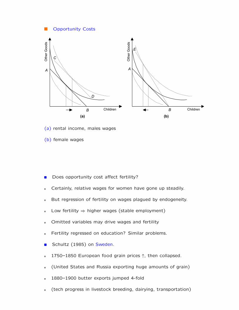
Opportunity Costs
(a) rental income, males wages
(b) female wages
0-16
Does opportunity cost a↵ect fertility?
Certainly, relative wages for women have gone up steadily.
But regression of fertility on wages plagued by endogeneity.
Low fertility ) higher wages (stable employment)
Omitted variables may drive wages and fertility
Fertility regressed on education? Similar problems.
Schultz (1985) on Sweden.
1750–1850 European food grain prices ", then collapsed.
(United States and Russia exporting huge amounts of grain)
1880–1900 butter exports jumped 4-fold
(tech progress in livestock breeding, dairying, transportation)
0-17
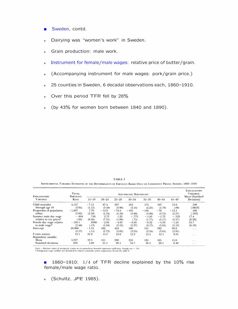
Sweden, contd.
Dairying was “women’s work” in Sweden.
Grain production: male work.
Instrument for female/male wages: relative price of butter/grain.
(Accompanying instrument for male wages: pork/grain price.)
25 counties in Sweden, 6 decadal observations each, 1860–1910.
Over this period TFR fell by 28%
(by 43% for women born between 1840 and 1890).
0-18
1860–1910: 1/4 of TFR decline explained by the 10% risefemale/male wage ratio.
(Schultz, JPE 1985).
0-19

Is Fertility Too High?
Three sources:
I. Incomplete information:
Umed Singh example; may not know that death rates declined.
II. Ex-ante versus ex-post:
“Too many” surviving children ex-post
(sounds cruel, but you get the drift)
III. Externalities:
Private gain/cost versus social gain/cost
0-20
Externality example 1. Education or health subsidies.
0-21
Externality example 2. Children as Lottery Tickets.
Say jobs are available for $1,000 per month.
Queue for such jobs.
Probability of getting job = total number of jobstotal number of job seekers .
An additional child = additional lottery ticket for the family.
But total number of job seekers goes up. Negative externality.
E↵ect is minuscule when one family does this.
But combined overall e↵ect is significant and negative.
) equilibrium fertility is higher than socially optimal.
0-22
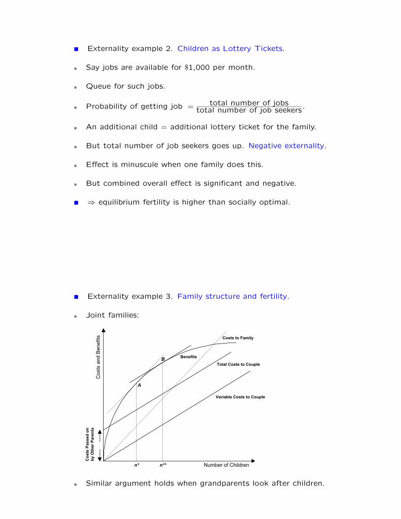
Externality example 3. Family structure and fertility.
Joint families:
Similar argument holds when grandparents look after children.
0-23
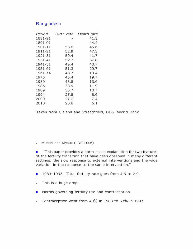
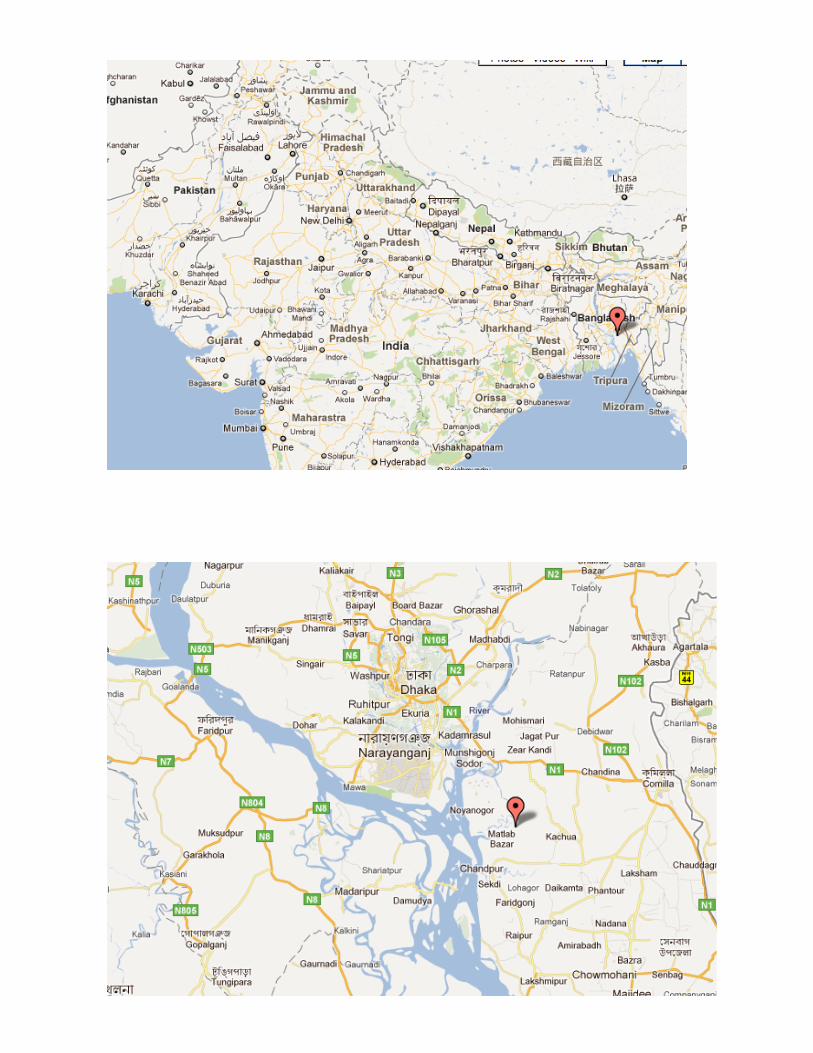
Bangladesh
Period Birth rate Death rate
1881-91 - 41.31891-01 - 44.41901-11 53.8 45.61911-21 52.9 47.31921-31 50.4 41.71931-41 52.7 37.81941-51 49.4 40.71951-61 51.3 29.71961-74 48.3 19.41976 45.4 19.71980 43.8 13.61986 38.9 11.91989 36.7 10.71994 27.8 8.62000 27.2 7.42010 20.8 6.1
Taken from Cleland and Streathfield, BBS, World Bank
Equilibrium Transition? Fertility Decline in Bangladesh
0-24
Munshi and Myaux (JDE 2006)
“This paper provides a norm-based explanation for two featuresof the fertility transition that have been observed in many di↵erentsettings: the slow response to external interventions and the widevariation in the response to the same intervention.”
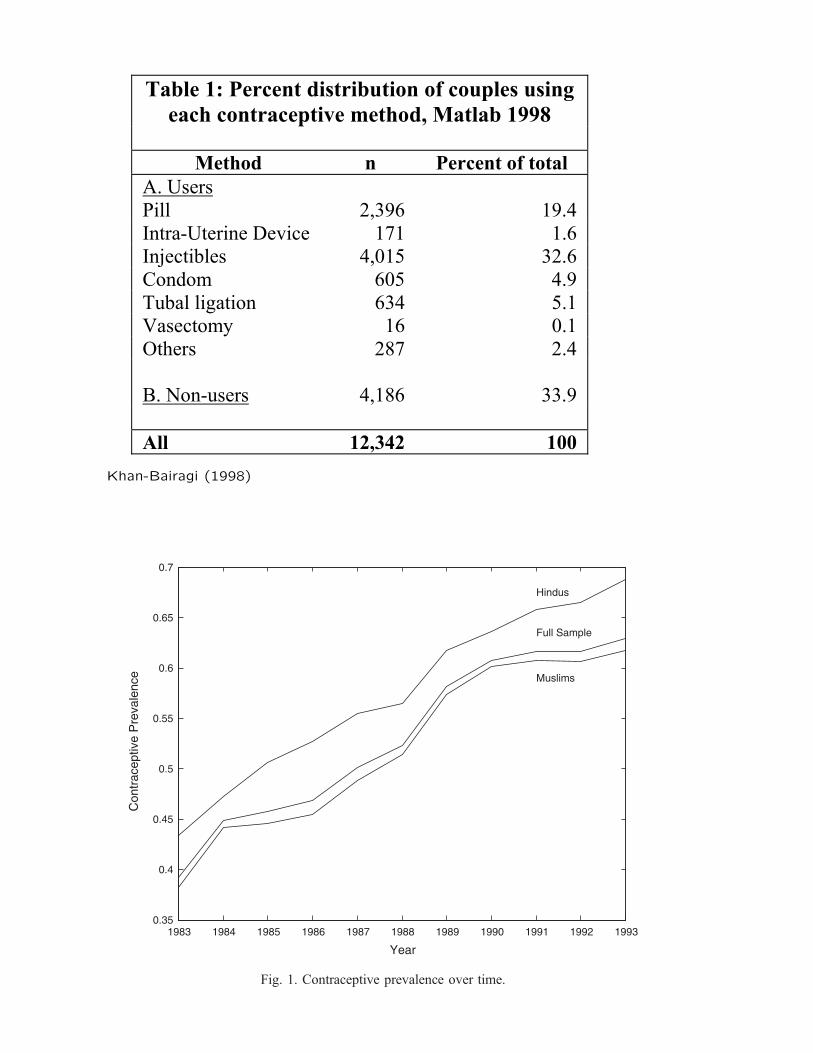
1983–1993: Total fertility rate goes from 4.5 to 2.9.
This is a huge drop.
Norms governing fertility use and contraception.
Contraception went from 40% in 1983 to 63% in 1993.
0-25
0-26
0-27

0-28
Maternal Child HealthFamily Planning (MCH-FP) project
Launched in 1978, 70 villages in Matlab thana, Comilla district.
Intensive family planning program
Community Health Worker (CHW) visited each family once ev-ery 2 weeks since start of the project in 1978.
Contraceptives are provided to them free of cost.
Use goes from from 40% in 1983 to 63% in 1993
TFR from 4.5 to 2.9 children over that period.
0-29
!"#$%&'(")(*+&',-(.(/"0#'&,1"%(1%(2+3+'"01%4(5"#%,$1+67(899:;(<=8>?:@A88(
<%)! #0/0$).! '*)! &+! ,&-.&/*! 0*! 4)$! $&! ?)!:0.)#4! 0-5)*$0(3$).;! JO0*$0-(! *$'.0)*! 12&50.)! *&/)! 0-.0,3$0&-*!3?&'$! :%4! ,&-.&/! '*)! 0*! #0/0$).! MC&#/3-! 3-.! "#3/9! FHHTN;! C&2! )O3/1#)9! -&$! +))#0-(! ,&/+&2$3?#)! .'20-(!0-$)2,&'2*)!0*!3!.0*,&'23(0-(!+3,$&2!0-!,&-.&/!'*3();!C))#0-(!*%4!3?&'$!1'2,%3*0-(!,&-.&/*!12)5)-$*!*&/)!'*)2*;!6$!:&'#.!?)!:&2$%:%0#)!$&!12&?)!.))1)2!0-$&!$%0*!0**')!&+!,'#$'23#!0-%0?0$0&-;!!6$!/34!?)!12)*'/).!$%3$!$%)!$3?&&!&-!+2))!*)O'3#!.0*,'**0&-!%3*!,&-$20?'$).!$&!3!*)-*)!&+!*%3/)!3?&'$!,&-.&/!'*3()a;!!!
,/($3"7.,,8&$(%*&0.,!
73$3!+&2!$%0*!*$'.4!,3/)!+2&/!$%)!E),&2.!R))10-(!84*$)/!MER8N!&+!$%)!>3$#3?!>3$)2-3#!3-.!@%0#.!A)3#$%BC3/0#4! D#3--0-(! M>@ABCDN! D2&^),$! 3-.! :3*! ,&##),$).! 0-! \,$&?)2! FHHY;! <%)! ER8! 0*! 3! /&-$%#4! .3$3! ,&##),$0&-!*4*$)/!3-.! $%)! 2)*1&-.)-$*! 0-,#'.)!3##!/3220).!:&/)-!&+!,%0#.?)320-(!3()! 0-! $%)!IG!*)#),$).!50##3()*!&+!>3$#3?;!!<%)*)!:&/)-!2),)05)! $%)!>@ABCD!0-$)25)-$0&-!?4!6@77E9=;!8'25)4!53203?#)*! 0-,#'.)!+3/0#4!1#3--0-(!*)250,)*9!*)#),$).!.)/&(231%0,!3-.!2)12&.',$05)!1323/)$)2*;!=0B53203$)!3-.!>'#$053203$)!3-3#4*)*!32)!)/1#&4).!+&2!$%0*!*$'.4;!!!
!=(.60$.,!
"!5320).!,&-$23,)1$05)!/)$%&.!/0O!0-!>3$#3?!2)5)3#*!3!'-0P')!+)3$'2)!$%3$!.0++)2*!+2&/!$%)!-3$0&-3#!13$$)2-;!<%)!#32()*$!.0*$0-,$0&-!#0)*!0-!0-^),$0?#)!,&-$23,)1$0&-!?)0-(!$%)!/&*$!12)53#)-$!,&-$23,)1$05)!/)$%&.;!
\-)!/&2)!.0*$0-('0*%0-(!+)3$'2)!&+!>3$#3?! 0*! 0$*!@&-$23,)1$05)!D2)53#)-,)!E3$)! M@DEN!b!XX;F!1)2,)-$! 0-!,&-$23*$!$&!ZG;T!1)2,)-$!3$!$%)!-3$0&-3#!#)5)#!M>0$23!)$!3#9!FHHIN;!=02$%!@&-$2&#!10##*!32)!*),&-.!$&!0-^),$0?#)*!0-!$)2/*!&+! '*3()! 23$)*;! @&-.&/*! 32)! 3#*&! '*).! 3$! 3! %0(%)2! #)5)#! $%3-! :%3$! 0*! +&'-.! 3$! $%)! -3$0&-3#! #)5)#! Ma;H! 1)2,)-$!,&/132).!$&!];H!1)2,)-$N;!=&$%!1)2/3-)-$!/)$%&.*!32)!'*).!3$!3!#)**)2!23$)!$%3-!+&'-.!3$!$%)!-3$0&-3#!#)5)#;![&/)-!3.&1$).!1)2/3-)-$!/)$%&.*!&+!,&-$23,)1$0&-!3$!3!%0(%)2!23$)!$%3-!/)-9!0/1#40-(!3!(2)3$)2!0-,#0-3$0&-!3/&-(!/3#)*!$&!2)$30-!,&-$2&#!&5)2!$%)02!2)12&.',$05)!,313,0$4;!<%)!12).&/0-3-,)!&+!+)/3#)!,&-$23,)1$05)!/)$%&.*!&5)23##!/34!3#*&!?)!*))-!3*!/3#)K*! 2)#',$3-,)! $&:32.*!,&-$23,)1$0&-;![%3$)5)2!%3**#)*!32)! 0-5).! 0-! $%)! 2&'$0-)!123,$0,)!&+!,&-$23,)1$05)!/)$%&.!32)!#32()#4!?&2-)!?4!$%)!:&/)-;!<%0*!0*!,&-*0*$)-$!:0$%!13$2032,%3#!,'#$'2)!-&2/*!$%3$!0/1&*)!(2)3$)2!?'2.)-!&-!:&/)-!0-!$%)!%&'*)%&#.;!!
!>&10(,?9,@(%'(#$,7*.$%*16$*"#,"A,'"6)0(.,6.*#B,(&'3,'"#$%&'()$*+(,8($3"7C,/&$0&1,?DDE,
! ! !/($3"7, #, @(%'(#$,"A,$"$&0,
";!W*)2*! ! !D0##! T9]HX! FH;a!6-$23BW$)20-)!7)50,)! FIF! F;X!6-^),$0?#)*! a9GFZ! ]T;X!@&-.&/! XGZ! a;H!<'?3#!#0(3$0&-! X]a! Z;F!S3*),$&/4! FX! G;F!\$%)2*! TYI! T;a!! ! !=;!c&-B'*)2*! a9FYX! ]];H!! ! !<00, ?FCGHF, ?II,
!<%)! '*)! &+! $%)! 10##9! 0-^),$0?#)*9! ,&-.&/*! 3-.! $'?3#! #0(3$0&-! 0-,2)3*)*!:0$%! $%)! 3()! &+! 3!/3220).!:&/3-;!!
<%)2)! 0*!*&/)!0-,&-*0*$)-,4!0-! $%)*)!2)*'#$*! ! M<3?#)TN;, ,E0*)*!3-.!.),#0-)*!&+!'*)! $3Q)!1#3,)!+2)P')-$#4!/3Q0-(! 0$!.0++0,'#$!$&!0.)-$0+4!3-4!/)$%&.!:0$%!3-4!132$0,'#32!3()!,&%&2$;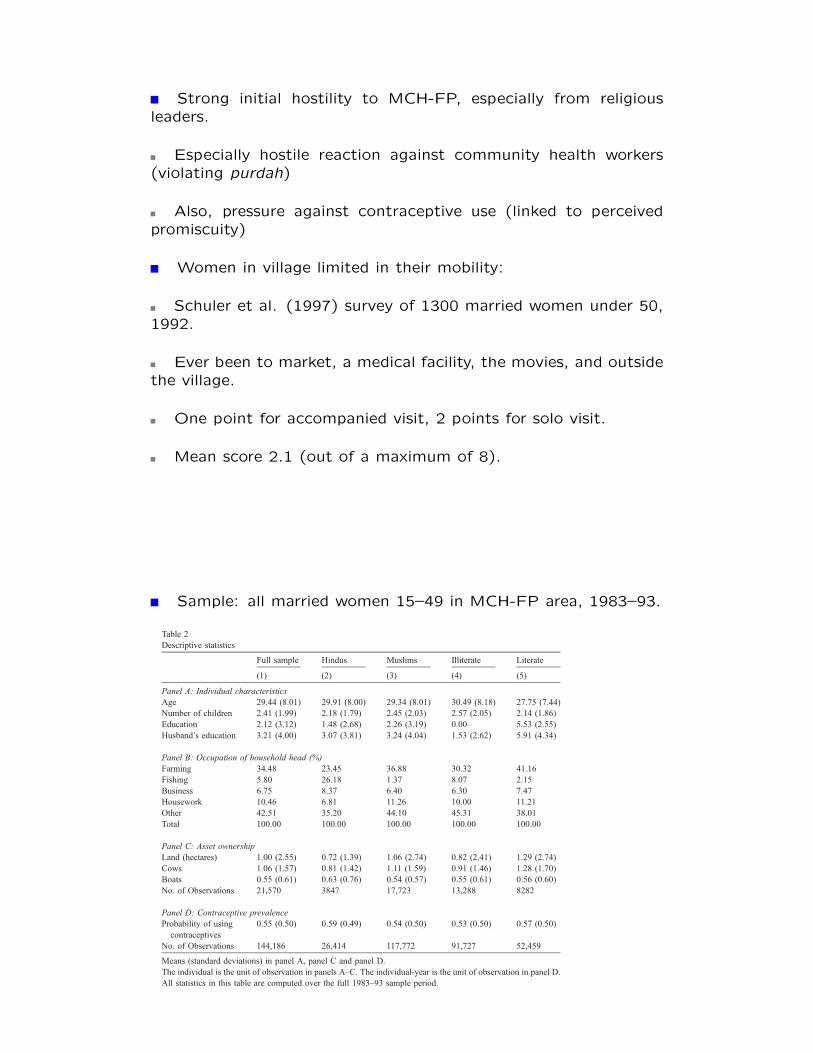
Strong initial hostility to MCH-FP, especially from religiousleaders.
Especially hostile reaction against community health workers(violating purdah)
Also, pressure against contraceptive use (linked to perceivedpromiscuity)
Women in village limited in their mobility:
Schuler et al. (1997) survey of 1300 married women under 50,1992.
Ever been to market, a medical facility, the movies, and outsidethe village.
One point for accompanied visit, 2 points for solo visit.
Mean score 2.1 (out of a maximum of 8).
0-32
Sample: all married women 15–49 in MCH-FP area, 1983–93.
While we could reject the hypothesis that the means across religious groups are equalfor most of the variables in Table 2, these statistics are generally of comparablemagnitude. The two religious groups display qualitatively similar demographiccharacteristics, occupational patterns, and asset ownership, yet we will later see whatappears to be absolutely no interaction, with regard to contraceptive use, within thevillage.
We complete this section by reporting average contraceptive prevalence, for the fullsample as well as for the different groups of women in panel D. Contraceptive prevalenceis roughly 55% over the sample period, and it is about 5 percentage points higher for theHindus and the literate women, relative to their respective comparison groups (thesedifferences are statistically significant).20
Table 2
Descriptive statistics
Full sample Hindus Muslims Illiterate Literate
(1) (2) (3) (4) (5)
Panel A: Individual characteristics
Age 29.44 (8.01) 29.91 (8.00) 29.34 (8.01) 30.49 (8.18) 27.75 (7.44)
Number of children 2.41 (1.99) 2.18 (1.79) 2.45 (2.03) 2.57 (2.05) 2.14 (1.86)
Education 2.12 (3.12) 1.48 (2.68) 2.26 (3.19) 0.00– 5.53 (2.55)
Husband’s education 3.21 (4.00) 3.07 (3.81) 3.24 (4.04) 1.53 (2.62) 5.91 (4.34)
Panel B: Occupation of household head (%)
Farming 34.48 23.45 36.88 30.32 41.16
Fishing 5.80 26.18 1.37 8.07 2.15
Business 6.75 8.37 6.40 6.30 7.47
Housework 10.46 6.81 11.26 10.00 11.21
Other 42.51 35.20 44.10 45.31 38.01
Total 100.00 100.00 100.00 100.00 100.00
Panel C: Asset ownership
Land (hectares) 1.00 (2.55) 0.72 (1.39) 1.06 (2.74) 0.82 (2.41) 1.29 (2.74)
Cows 1.06 (1.57) 0.81 (1.42) 1.11 (1.59) 0.91 (1.46) 1.28 (1.70)
Boats 0.55 (0.61) 0.63 (0.76) 0.54 (0.57) 0.55 (0.61) 0.56 (0.60)
No. of Observations 21,570 3847 17,723 13,288 8282
Panel D: Contraceptive prevalence
Probability of using
contraceptives
0.55 (0.50) 0.59 (0.49) 0.54 (0.50) 0.53 (0.50) 0.57 (0.50)
No. of Observations 144,186 26,414 117,772 91,727 52,459
Means (standard deviations) in panel A, panel C and panel D.
The individual is the unit of observation in panels A–C. The individual-year is the unit of observation in panel D.
All statistics in this table are computed over the full 1983–93 sample period.
20 Annual (December 31) data are used to compute the statistics in panel D. The number of observations in panel
D is larger than the number of observations in the regressions that we report later using annual data because we
compute all the statistics in panel D over the full 1983–93 sample period. In contrast, we must drop the first year
(1983) in the regressions since the lagged decision and lagged contraceptive prevalence are included as regressors.
K. Munshi, J. Myaux / Journal of Development Economics 80 (2006) 1–3822
0-33
A Conceptual Problem
Linear probability model (also tried logit):
yit = A+ �yi,t�1 + �x
v(i)t�1 + ⌘Zit +C
v(i)t + ✏ivt
yi is 0-1 for contraceptive use by couple i, t is time, x is ag-gregate village-level use, v(i) is the village of person i, Z a vectorof individual characteristics (such as age) including individual andtime fixed e↵ects in some specifications.
C
vt is unobserved omitted variable for village v at date t.
At the heart of identification problem (Manski critique)
� can pick up the e↵ects of unobserved C
vt . . .
E.g., economic growth
Village-level success of the MCH-FP program.
0-34
C
v
t
C
vt can be decomposed into three parts.
First component only depends on the village: C
v1 .
Second component only depends on time: Ct2.
Third varies in a village-specific way over time.
Components 1 and 2 dealt with by village and time fixed e↵ects.
The last one screws everything up: identification problem.
0-35

Main Idea in Munshi-Myaux Paper
Inter-religion communication low.
So include own-group and cross-group use separately.
If own-e↵ect strong, then pushes back the Manski critique:
For critique to work, there has to be an omitted variable whichis village-, time- and group-specific.
yit = A+ �myi,t�1 + �mmx
v(i),mt�1 ++�mhx
v(i),ht�1 + ⌘mZit +C
v(i),mt + ✏ivt
where i is m-household, and m and h labels self-explanatory.
Can get spurious e↵ects only if C
v(i),mt and C
v(i),ht orthogonal.
0-36
Muslims, in most of the specifications that we consider in this section. Age and agesquared are included as control variables. The coefficient on the individual’s age ispositive, the coefficient on age squared is negative, and both these coefficients are veryprecisely estimated, without exception.
The first regression in Columns 1–2 of Table 3 considers all villages and we see thatstrong within-religion effects are obtained, while cross-religion effects are entirely absent,both for Hindus and Muslims. While these results are very promising, one cause forconcern is that villages may be predominantly of one religion or the other. In the extremecase, all the within-religion effects could be obtained from villages that consist exclusivelyof households belonging to a particular religion, which would leave no room at all forcross-religion effects. Although we do not see this sort of segregation in the data, somevillages are dominated by a single religion. We consequently proceed to remove allvillages with less than 5% Hindus or Muslims from the sample in Columns 3–4.Thereafter, we discard villages with less than 15% Hindus or Muslims in Columns 5–6.The sample size declines substantially over the course of this exercise, and is less than halfthe size of what we began with. Yet we see that the estimated within-religion and cross-religion effects, for both Hindus and Muslims, remain remarkably stable across thedifferent sample sizes in Table 3.24
Table 3
Partitioning the village by religion
Dependent variable: contraception
All villages More than 5%
Hindus/Muslims
More than 15%
Hindus/Muslims
Annual data
Muslims Hindus Muslims Hindus Muslims Hindus Muslims Hindus
(1) (2) (3) (4) (5) (6) (7) (8)
Lagged contraceptive
prevalence (own group)
0.217
(0.013)
0.161
(0.014)
0.193
(0.016)
0.169
(0.017)
0.207
(0.018)
0.168
(0.020)
0.312
(0.023)
0.246
(0.023)
Lagged contraceptive
prevalence (other group)
0.008
(0.006)
0.009
(0.007)
0.007
(0.011)
0.024
(0.016)
! 0.001
(0.013)
0.019
(0.024)
0.009
(0.011)
0.006
(0.012)
Lagged contraception 0.698
(0.003)
0.712
(0.005)
0.704
(0.004)
0.710
(0.005)
0.706
(0.004)
0.717
(0.006)
0.498
(0.005)
0.517
(0.008)
R2 0.513 0.559 0.520 0.558 0.521 0.565 0.281 0.338
Number of observations 139,875 43,101 79,927 29,771 49,730 20,756 70,787 21,419
Box–Pearson Q statistic 0.000 0.003 0.001 0.002 0.002 0.006 0.003 0.008
Standard errors in parentheses.
Standard errors are robust to heteroskedasticity and correlated residuals within each village-period.
Q ~X12 under H0: no serial correlation. The critical value above which the null is rejected at the 5% significance
level is 3.84.
Columns 1–2: Sample includes all mixed-religion villages.
Columns 3–4: Sample restricted to villages with more than 5% Hindus and Muslims.
Columns 5–6: Sample restricted to villages with more than 15% Hindus and Muslims.
Columns 7–8: Annual data.
24 In a related robustness test, we also verified that the size of the village, measured by the total number of
eligible women, has no effect on the estimated within-religion and cross-religion effects.
K. Munshi, J. Myaux / Journal of Development Economics 80 (2006) 1–3826
All data 6-monthly except last two columns
See paper for other robustness checks: no fisherman, bari-level e↵ects
0-37

Alternative Explanations
Program e↵ects:
Cross-sectional variation: individual fixed e↵ects.
Secular changes: time e↵ects.
But village-specific time e↵ects pose a problem. The CHWvaries from village to village, after all.
That is where the own-religion cross-religion trick plays a role.
Economic growth
Religion and occupation largely uncorrelated except for fisher-men.
Learning about a new technology
Possible, with injectibles. But authors argue against it.
0-38
Related Documents


![arXiv:1808.00659v1 [cs.CR] 2 Aug 2018 · New York University huzh@nyu.edu Yu Hu New York University yh570@nyu.edu Brendan Dolan-Gavitt New York University brendandg@nyu.edu Abstract—Sophisticated](https://static.cupdf.com/doc/110x72/5c64ffa409d3f2826e8c03eb/arxiv180800659v1-cscr-2-aug-2018-new-york-university-huzhnyuedu-yu-hu.jpg)

