CSE-801: Stochastic Systems Analysis and Processing of Random Variables Syed Ali Khayam Syed Ali Khayam School of Electrical Engineering & Computer Science National University of Sciences & Technology (NUST) Pakistan Copyright © Syed Ali Khayam 2008

Welcome message from author
This document is posted to help you gain knowledge. Please leave a comment to let me know what you think about it! Share it to your friends and learn new things together.
Transcript
CSE-801: Stochastic Systems
Analysis and Processing of Random Variables
Syed Ali KhayamSyed Ali KhayamSchool of Electrical Engineering & Computer ScienceNational University of Sciences & Technology (NUST)Pakistan
Copyright © Syed Ali Khayam 2008

What will we cover in this lecture?
In this lecture, we will cover:Functions of a Random VariableMoments of a Random VariableMoments of a Random VariableTransform Domain Methods
Copyright © Syed Ali Khayam 2008 2
F ti f R d V i blFunctions of a Random Variable
Copyright © Syed Ali Khayam 2008 3
Functions of a Random VariableIn practical problems, sometimes you know the distributions of random inputs and the function that maps the inputs to outputs
I h bl t t th d i blIn such problems, we cannot operate on the random variables directly
Instead, we have to work with a function, g(X1, X2,…,Xn), of the , , g( 1, 2, , n),random inputs X1, X2,…,Xn
Copyright © Syed Ali Khayam 2008 4
Functions of a Random Variable
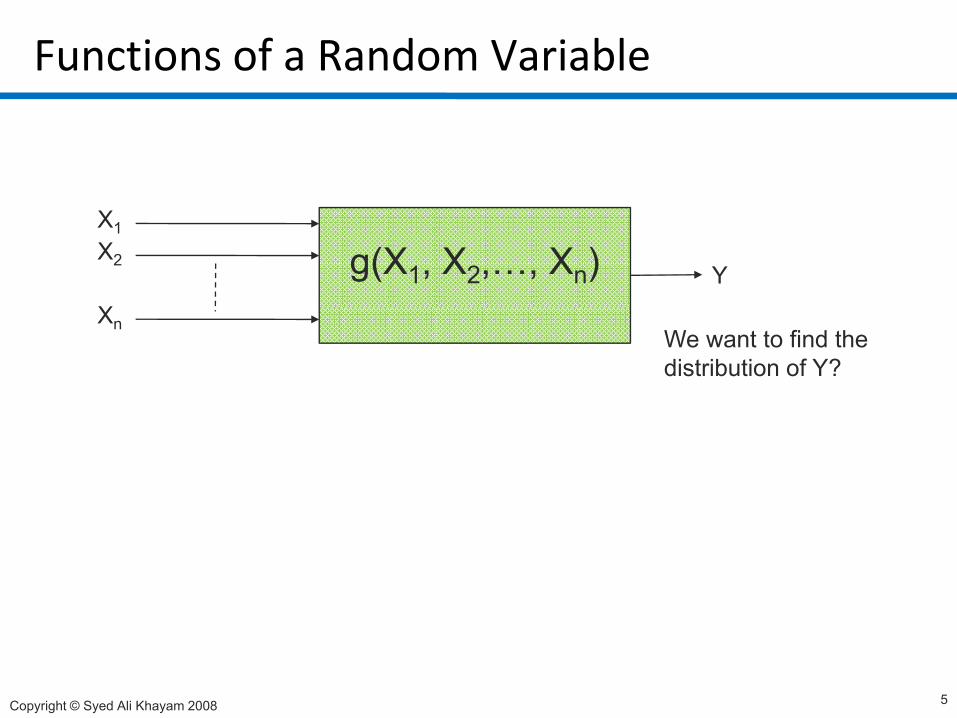
g(X1, X2,…, Xn)X1X2
X
Y
XnWe want to find the distribution of Y?
Copyright © Syed Ali Khayam 2008 5
Functions of a Random Variable
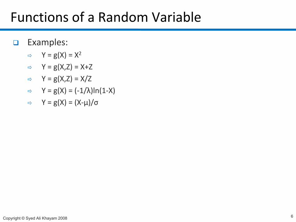
Examples:Y = g(X) = X2
Y = g(X,Z) = X+Z
Y = g(X,Z) = X/Z
Y = g(X) = (-1/λ)ln(1-X)
Y = g(X) = (X-μ)/σ
Copyright © Syed Ali Khayam 2008 6
Functions of a Random VariableTo develop intuition, let us focus on functions of a single random variable
Y g(X) X2 where X~EXP(λ)Y = g(X) = X2, where X~EXP(λ)
Y = g(X) = (X-μ)/σ, where X~N(μ, σ2)
Copyright © Syed Ali Khayam 2008 7
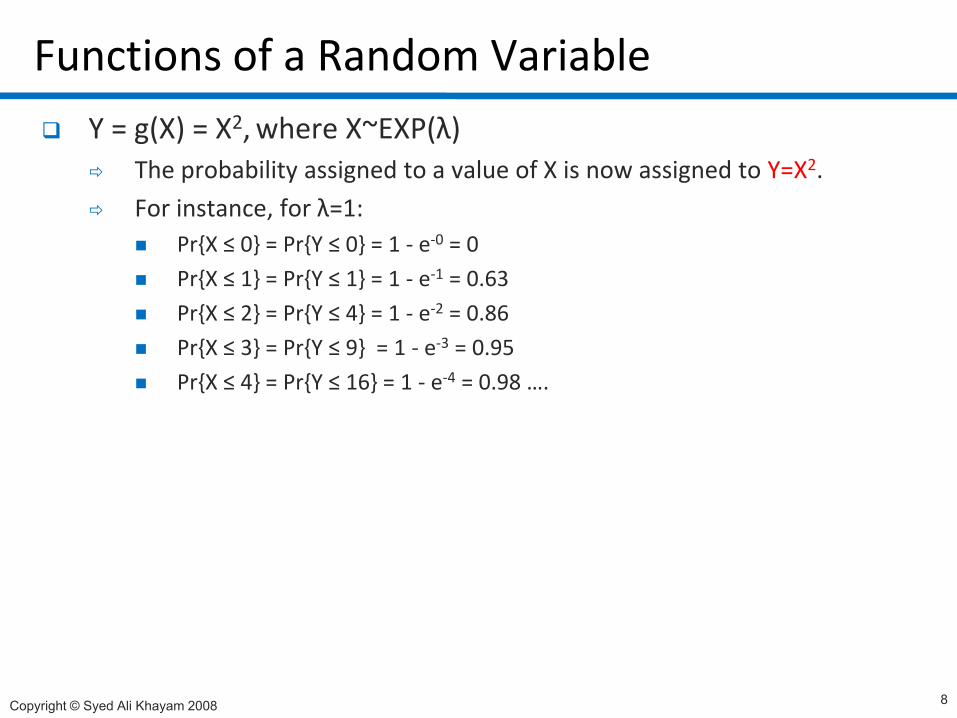
Functions of a Random VariableY = g(X) = X2, where X~EXP(λ)
The probability assigned to a value of X is now assigned to Y=X2.
For instance for λ 1:For instance, for λ=1:Pr{X ≤ 0} = Pr{Y ≤ 0} = 1 - e-0 = 0
Pr{X ≤ 1} = Pr{Y ≤ 1} = 1 - e-1 = 0.63
P {X ≤ 2} P {Y ≤ 4} 1 2 0 86Pr{X ≤ 2} = Pr{Y ≤ 4} = 1 - e-2 = 0.86
Pr{X ≤ 3} = Pr{Y ≤ 9} = 1 - e-3 = 0.95
Pr{X ≤ 4} = Pr{Y ≤ 16} = 1 - e-4 = 0.98 ….
Copyright © Syed Ali Khayam 2008 8
Functions of a Random Variable
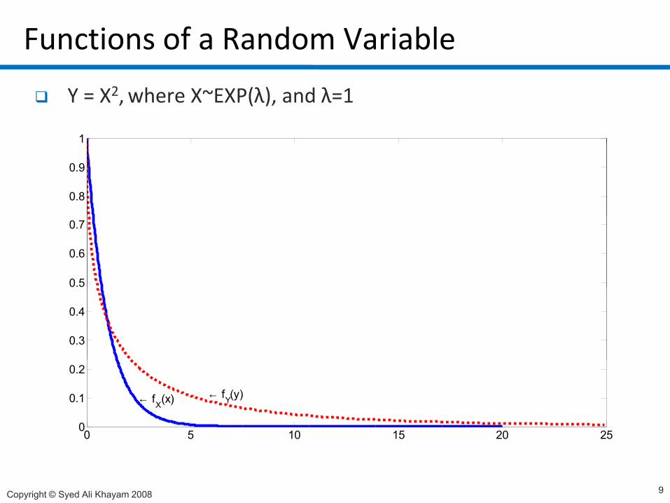
Y = X2, where X~EXP(λ), and λ=1
1
0.8
0.9
0.5
0.6
0.7
0.3
0.4
0 5 10 15 20 250
0.1
0.2
← fX(x) ← fY(y)
Copyright © Syed Ali Khayam 2008
0 5 10 15 20 250
9
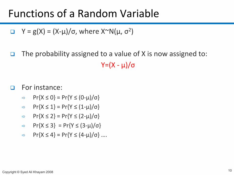
Functions of a Random VariableY = g(X) = (X-μ)/σ, where X~N(μ, σ2)
The probability assigned to a value of X is now assigned to:
Y=(X - μ)/σ
For instance:Pr{X ≤ 0} = Pr{Y ≤ (0-μ)/σ}{ } { ( μ)/ }
Pr{X ≤ 1} = Pr{Y ≤ (1-μ)/σ}
Pr{X ≤ 2} = Pr{Y ≤ (2-μ)/σ}
Pr{X ≤ 3} = Pr{Y ≤ (3 μ)/σ}Pr{X ≤ 3} = Pr{Y ≤ (3-μ)/σ}
Pr{X ≤ 4} = Pr{Y ≤ (4-μ)/σ} ….
Copyright © Syed Ali Khayam 2008 10
Functions of a Random Variable
0.18
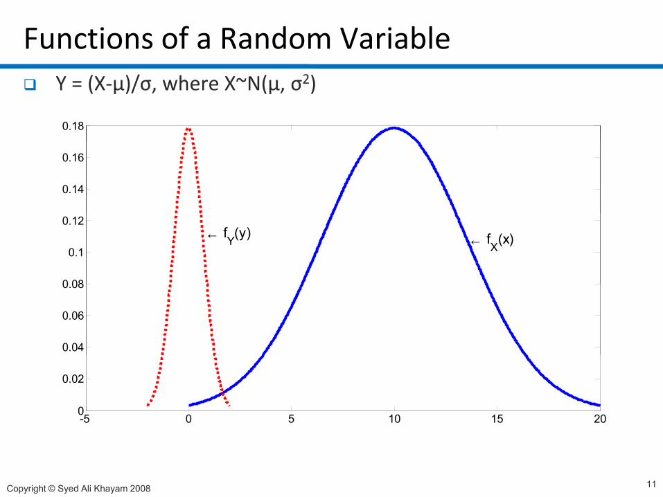
Y = (X-μ)/σ, where X~N(μ, σ2)
0.14
0.16
0 08
0.1
0.12
← fX(x)← fY(y)
0.04
0.06
0.08
-5 0 5 10 15 200
0.02
Copyright © Syed Ali Khayam 2008 11
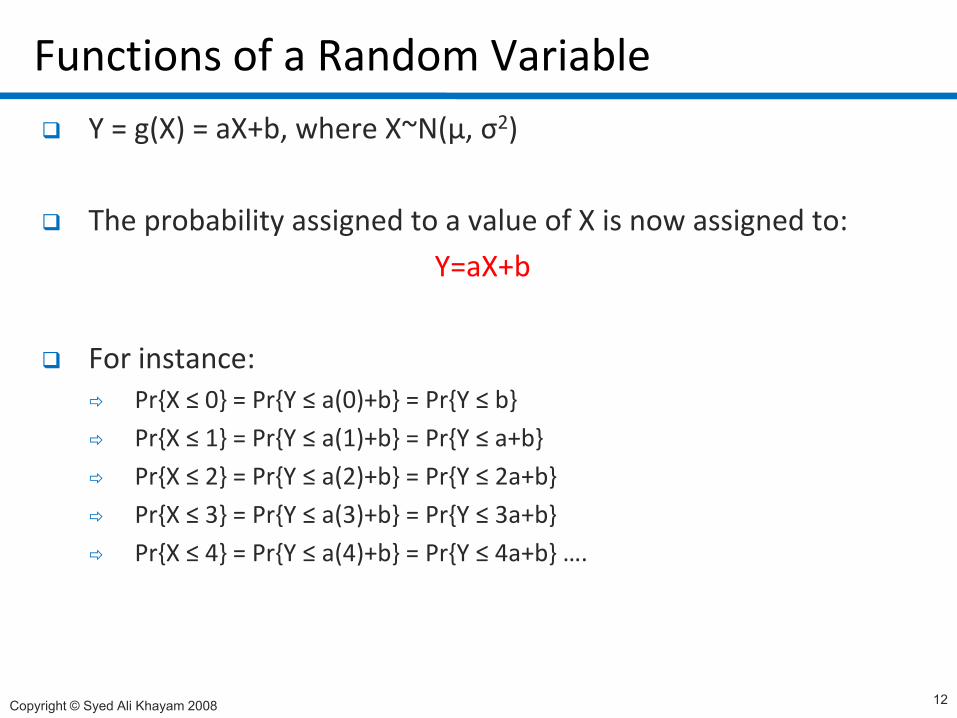
Functions of a Random VariableY = g(X) = aX+b, where X~N(μ, σ2)
The probability assigned to a value of X is now assigned to:
Y=aX+b
For instance:Pr{X ≤ 0} = Pr{Y ≤ a(0)+b} = Pr{Y ≤ b}{ } { ( ) } { }
Pr{X ≤ 1} = Pr{Y ≤ a(1)+b} = Pr{Y ≤ a+b}
Pr{X ≤ 2} = Pr{Y ≤ a(2)+b} = Pr{Y ≤ 2a+b}
Pr{X ≤ 3} = Pr{Y ≤ a(3)+b} = Pr{Y ≤ 3a+b}Pr{X ≤ 3} = Pr{Y ≤ a(3)+b} = Pr{Y ≤ 3a+b}
Pr{X ≤ 4} = Pr{Y ≤ a(4)+b} = Pr{Y ≤ 4a+b} ….
Copyright © Syed Ali Khayam 2008 12
Functions of a Random VariableWe need a mathematical measure of generating pdf and CDF of a function of a rv
To that end, we always start with the CDF of the random inputs and try to determine the CDF of the output
Copyright © Syed Ali Khayam 2008 13
Example1: Functions of a Random Variable
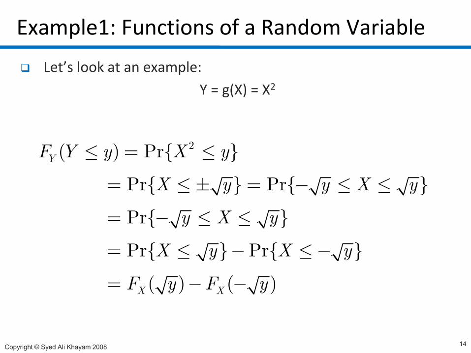
Let’s look at an example:
Y = g(X) = X2
2( ) Pr{ }F Y y X y≤ = ≤( ) Pr{ }
Pr{ } Pr{ }YF Y y X y
X y y X y
≤ = ≤
= ≤ ± = − ≤ ≤
Pr{ }
Pr{ } Pr{ }
y X y
X y X y
= − ≤ ≤
= ≤ − ≤−Pr{ } Pr{ }
( ) ( )X X
X y X y
F y F y
= ≤ − ≤−
= − −
Copyright © Syed Ali Khayam 2008 14
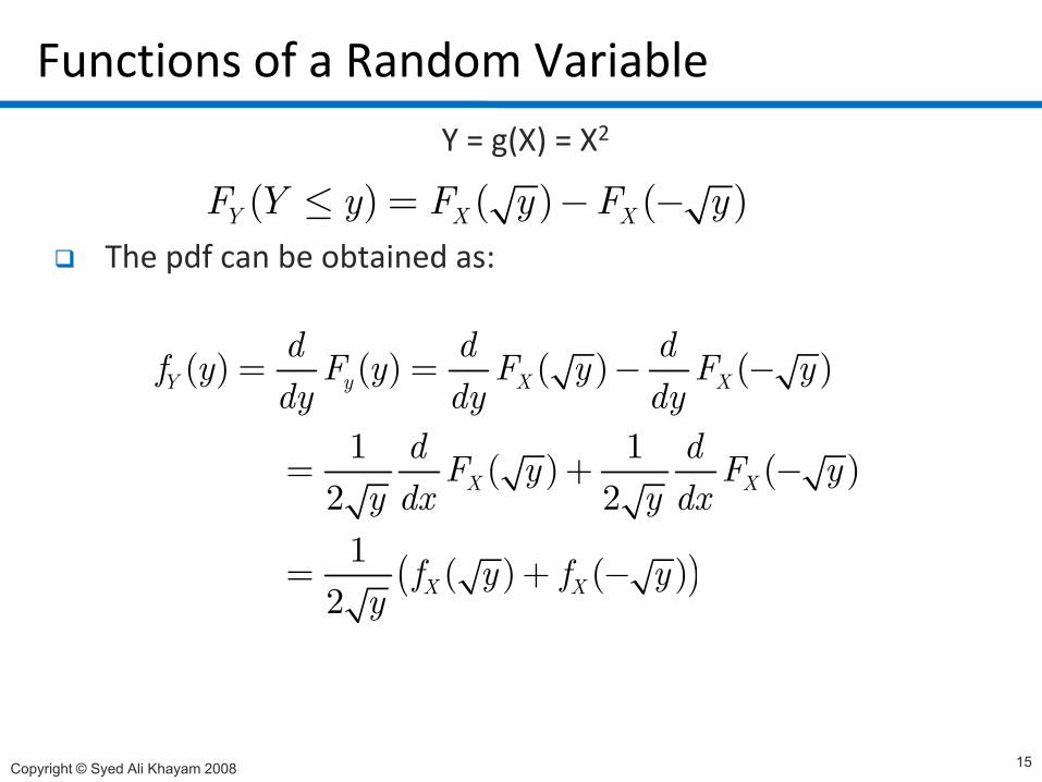
Functions of a Random VariableY = g(X) = X2
( ) ( ) ( )Y X XF Y y F y F y≤ = − −The pdf can be obtained as:
( ) ( ) ( )Y X X
d d d( ) ( ) ( ) ( )
1 1
Y y X Xd d df y F y F y F ydy dy dy
d d
= = − −
( )
1 1( ) ( )2 21 ( ) ( )
X Xd dF y F y
y dx y dx= + −
( )1 ( ) ( )2 X Xf y f yy
= + −
Copyright © Syed Ali Khayam 2008 15
Functions of a Random Variable
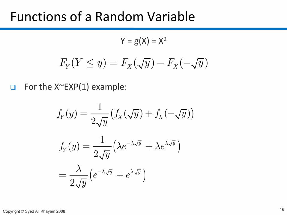
Y = g(X) = X2
( ) ( ) ( )F Y y F y F y≤
For the X~EXP(1) example:
( ) ( ) ( )Y X XF Y y F y F y≤ = − −
( )1( ) ( ) ( )2Y X Xf y f y f yy
= + −2 y
( )1( )2
y yYf y e e
yλ λλ λ−= +
( )2
2y y
y
e ey
λ λλ −= +
Copyright © Syed Ali Khayam 2008
2 y
16
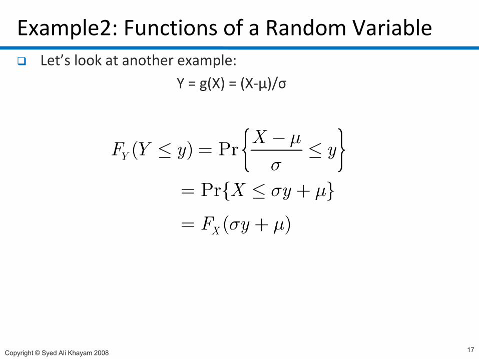
Example2: Functions of a Random VariableLet’s look at another example:
Y = g(X) = (X-μ)/σ
{ }( ) PrYXF Y y yµ−≤ = ≤{ }( ) Pr
Pr{ }
YF Y y y
X yσσ µ
≤ ≤
= ≤ +
( )XF yσ µ= +
Copyright © Syed Ali Khayam 2008 17
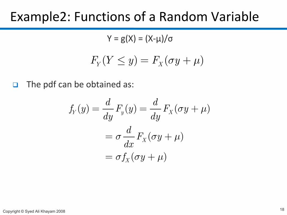
Example2: Functions of a Random VariableY = g(X) = (X-μ)/σ
( ) ( )F Y y F yσ µ≤ = +
The pdf can be obtained as:
( ) ( )Y XF Y y F yσ µ≤ = +
( ) ( ) ( )Y y Xd df y F y F ydy dy
σ µ= = +
( )
( )
Xd F ydxf
σ σ µ= +
( )Xf yσ σ µ= +
Copyright © Syed Ali Khayam 2008 18
Example2: Functions of a Random Variable
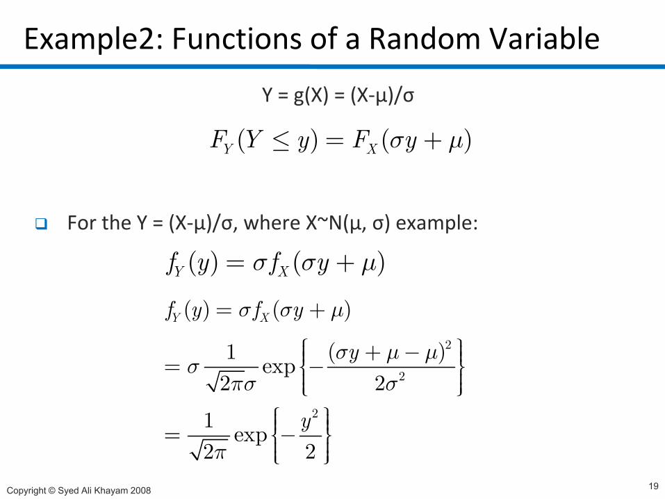
Y = g(X) = (X-μ)/σ
( ) ( )F Y y F yσ µ≤ = +
/
( ) ( )Y XF Y y F yσ µ≤ = +
For the Y = (X-μ)/σ, where X~N(μ, σ) example:
( ) ( )Y Xf y f yσ σ µ= +
2
( ) ( )
( )1
Y Xf y f y
y
σ σ µ
σ µ µ
= +
+ − 2
2
( )1 exp22
1
y
y
σ µ µσσπσ+ = −
Copyright © Syed Ali Khayam 2008
exp22y
π = −
19

Example2: Functions of a Random Variable
( ) ( )Y XF Y y F yσ µ≤ = +
For the Y = (X-μ)/σ, where X~N(μ, σ) example:
( ) ( )f f( ) ( )Y Xf y f yσ σ µ= +
( ) ( )Y Xf y f yσ σ µ= +2
2
( )1 exp22
yσ µ µσσπσ
+ − = − Gaussian rv with zero mean and unit variance: Standard
21 exp22y
π
= −
Copyright © Syed Ali Khayam 2008
variance: Standard Normal Distribution
20
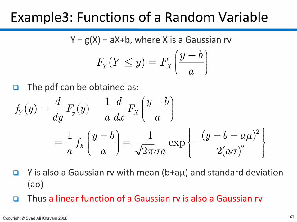
Example3: Functions of a Random VariableY = g(X) = aX+b, where X is a Gaussian rv
( ) y bF Y y F − ≤ =
The pdf can be obtained as:
( )Y XF Y y Fa
≤ =
1( ) ( )Y y Xd d y bf y F y Fdy a dx a
− = = 2
2
( )1 1 exp2( )2X
y b ay bfa a aa
µσπσ
− −− = = − Y is also a Gaussian rv with mean (b+aμ) and standard deviation (aσ)
Copyright © Syed Ali Khayam 2008
Thus a linear function of a Gaussian rv is also a Gaussian rv
21
Expected Value of a Function of a Random Variable
A function of a random variable is also a random variable
So how do we find the expected value of a function g(X) of aSo how do we find the expected value of a function g(X) of a random variable X?
Copyright © Syed Ali Khayam 2008 22
Expected Value of a Function of a Random Variable
How do we find the expected value of a function g(X) of a random variable X?
We can of course find the pdf or pmf of the function and then use the expectation formula to find its mean
However, there is a more direct method for finding the expected value of g(X)expected value of g(X)
Copyright © Syed Ali Khayam 2008 23
Expected Value of a Function of a Random Variable
How do we find the expected value of a function of a random variable?
Recall that expected value is simply a weighted average
Therefore, the expected value of a function g(X) of a discrete random variable X is a weighted average of the values taken by g(X=x)
The weights are the probabilities of these values in X
{ }( ) ( )Pr{ }k kk
E g X g X x X x= = =∑∑
Copyright © Syed Ali Khayam 2008 24
( ) ( )k X kk
g x p x=∑
Expected Value of a Function of a Random Variable
Expected value of a function g(X) of a discrete random variable X is
{ }( ) ( ) ( )k X kk
E g X g x p x=∑
Similarly, for a continuous rv, the expected value is given by
{ }∞
∫{ }( ) ( ) ( )XE g X g x f x dx−∞
= ∫
Copyright © Syed Ali Khayam 2008 25
Detour: “Useful” Properties of Expected ValueFor a constant value c,
l
{ }E c c=
{ } { }E X E XFor a constant value c,
For a sum of functions of random variables Y=X1+X2+…+X ,
{ } { }E cX cE X=
For a sum of functions of random variables Y X1+X2+…+Xn,
{ } ( ) { ( )}n n
k kE Y E g X E g X = = ∑ ∑{ }
1 1k k= = ∑ ∑
Copyright © Syed Ali Khayam 2008 26
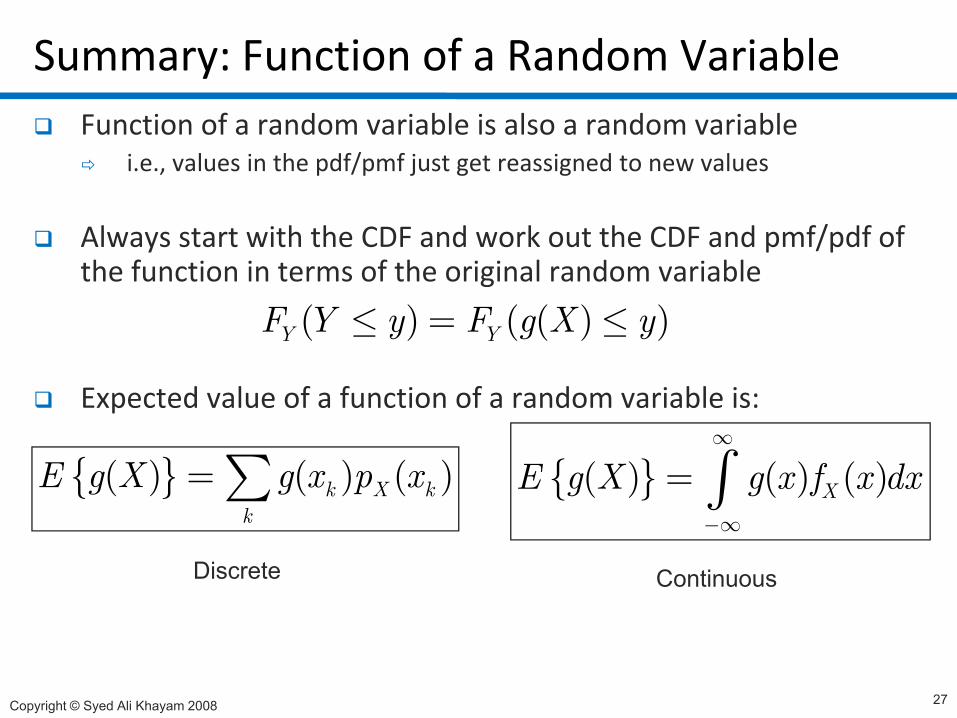
Summary: Function of a Random VariableFunction of a random variable is also a random variable
i.e., values in the pdf/pmf just get reassigned to new values
Always start with the CDF and work out the CDF and pmf/pdf of the function in terms of the original random variable
( ) ( ( ) )F Y F X
Expected value of a function of a random variable is:
( ) ( ( ) )Y YF Y y F g X y≤ = ≤
p
{ }( ) ( ) ( )k X kk
E g X g x p x=∑ { }( ) ( ) ( )XE g X g x f x dx∞
= ∫k −∞
Discrete Continuous
Copyright © Syed Ali Khayam 2008 27
HomeworkTextbook Problems
3.513.533.533.563.58
Copyright © Syed Ali Khayam 2008 28

M t f R d V i blMoments of a Random Variable
Copyright © Syed Ali Khayam 2008 29
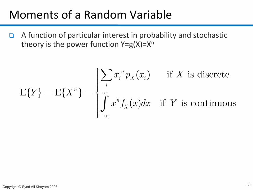
Moments of a Random Variable
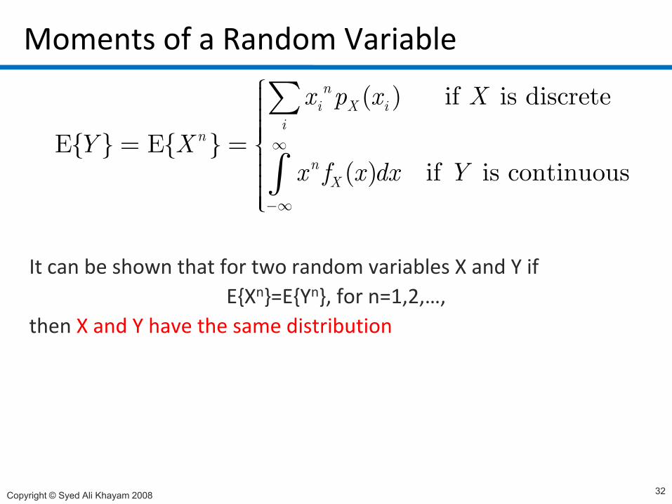
A function of particular interest in probability and stochastic theory is the power function Y=g(X)=Xn
( ) if is discreteni X ix p x X∑
{ } { }( ) if is continuous
in
nX
Y Xx f x dx Y
∞
Ε = Ε = ∫−∞∫
Copyright © Syed Ali Khayam 2008 30
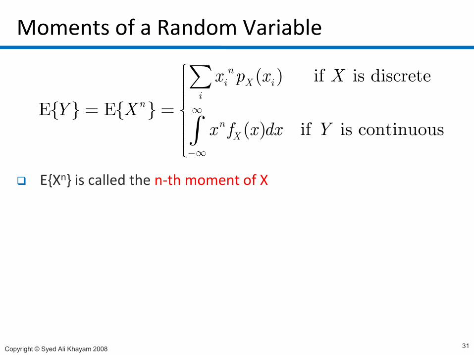
Moments of a Random Variable
( ) if is discreteni X i
i
x p x X∑
{ } { }( ) if is continuous
n
nX
Y Xx f x dx Y
∞
∞
Ε = Ε = ∫
E{Xn} is called the n-th moment of X
−∞
Copyright © Syed Ali Khayam 2008 31
Moments of a Random Variable
( ) if is discrete
{ } { }
ni X i
in
x p x X
Y X ∞
Ε = Ε =
∑{ } { }
( ) if is continuousnX
Y Xx f x dx Y
∞
−∞
Ε = Ε = ∫
It can be shown that for two random variables X and Y if { } { }E{Xn}=E{Yn}, for n=1,2,…,
then X and Y have the same distribution
Copyright © Syed Ali Khayam 2008 32
Representing Variance in terms of Moments
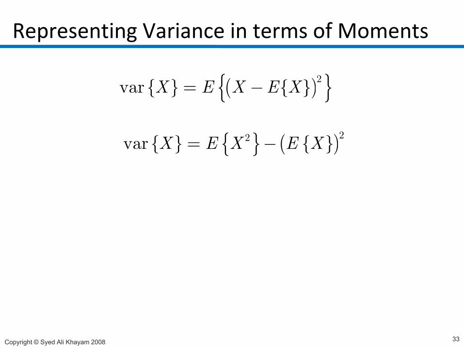
{ } ( ){ }2var { }X E X E X= −{ }
{ } { } { }( )22var X E X E X= −{ } { } { }( )
Copyright © Syed Ali Khayam 2008 33
Representing Variance in terms of Moments
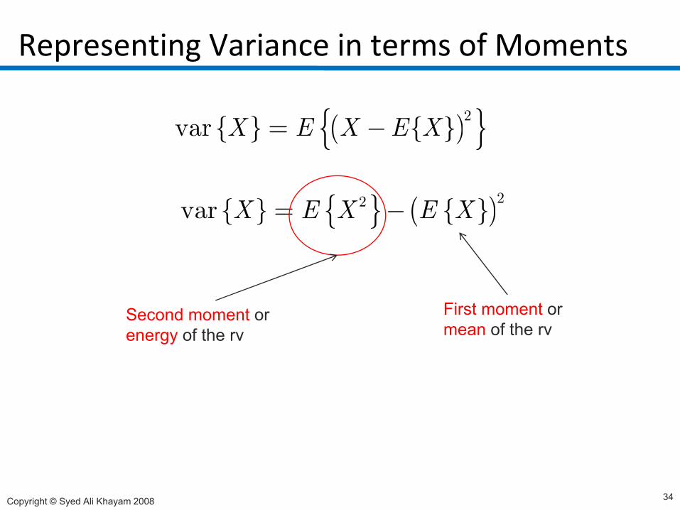
{ } ( ){ }2var { }X E X E X= −{ }
{ } { } { }( )22var X E X E X= −{ } { } { }( )
Second moment or energy of the rv
First moment or mean of the rv
Copyright © Syed Ali Khayam 2008 34
HomeworkTextbook Problems
3.713.743.743.76
Copyright © Syed Ali Khayam 2008 35

T f D i M th dTransform Domain Methods
Copyright © Syed Ali Khayam 2008 36
Transform Domain Methods
In signal processing and communications, it is sometimes beneficial to look at system variables in a transform or frequency domaindomain
Frequency domain representation allows one to simplify the analysis of a given signal or functionanalysis of a given signal or function
We will now cover two transform functions that are commonly used in stochastic literature:
Characteristic FunctionProbability Generating Function
Copyright © Syed Ali Khayam 2008 37
Characteristic Function of a Continuous RV
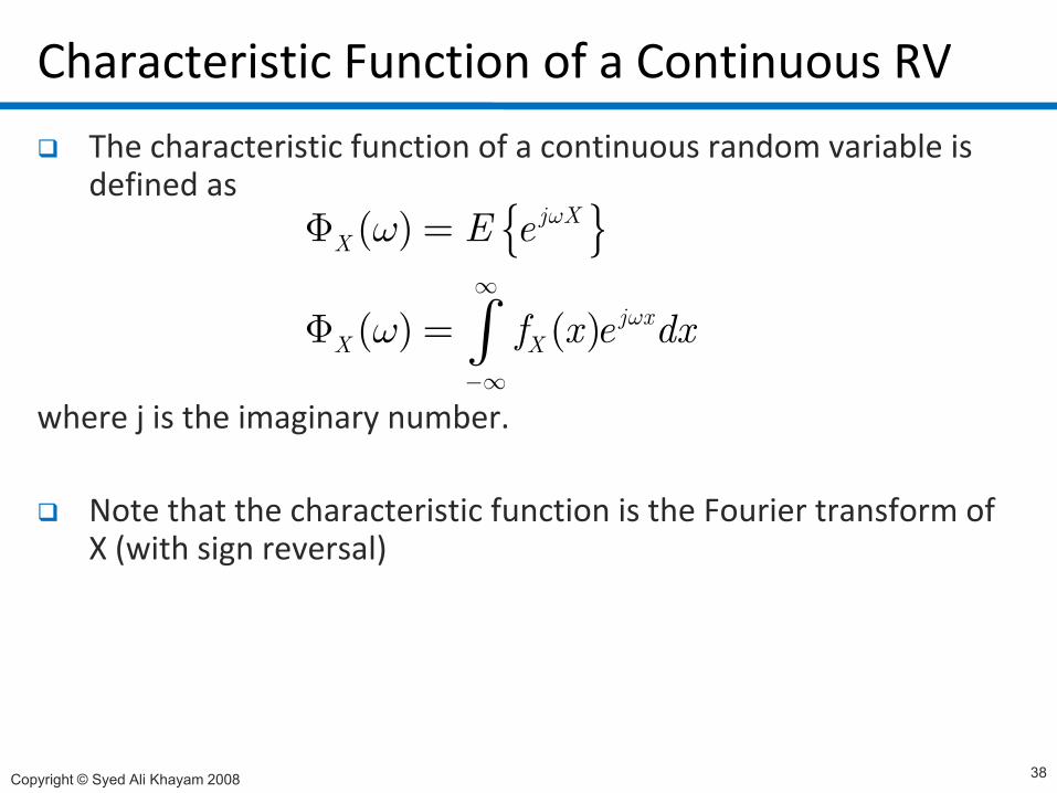
The characteristic function of a continuous random variable is defined as
{ }( ) j XE e ωωΦ = { }( )
( ) ( )
jX
j xX X
E e
f x e dxω
ω
ω∞
Φ =
Φ = ∫where j is the imaginary number.
( ) ( )X Xf x e dxω−∞
Φ ∫
Note that the characteristic function is the Fourier transform of X (with sign reversal)
Copyright © Syed Ali Khayam 2008 38
Characteristic Function of a Continuous RV
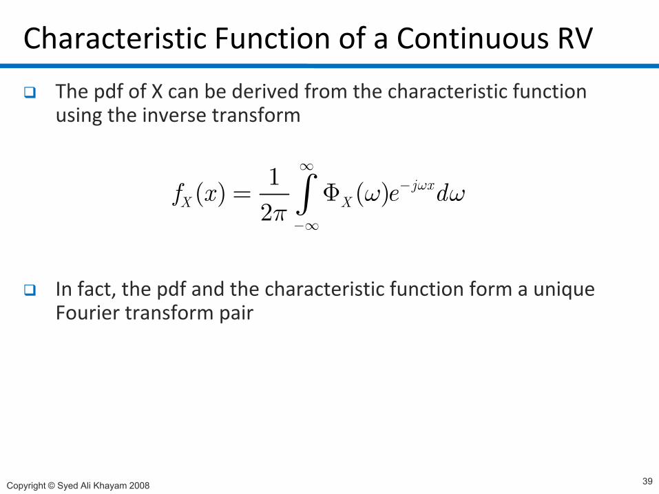
The pdf of X can be derived from the characteristic function using the inverse transform
1( ) ( )2
j xX Xf x e dωω ω
π
∞−= Φ∫
I f h df d h h i i f i f i
2π −∞∫
In fact, the pdf and the characteristic function form a unique Fourier transform pair
Copyright © Syed Ali Khayam 2008 39
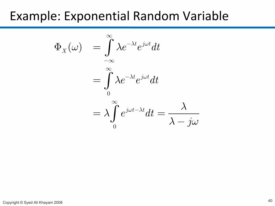
Example: Exponential Random Variable
( ) t j tX e e dtλ ωω λ
∞−Φ = ∫t j te e dtλ ωλ
−∞∞
−= ∫0
j t te dtj
ω λ λλλ
∞−= =
∫
∫0
jλ ω−∫
Copyright © Syed Ali Khayam 2008 40
Characteristic Function of a Discrete RV
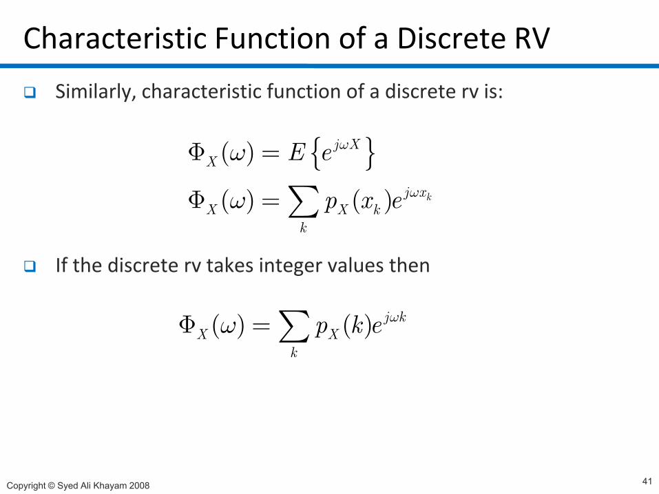
Similarly, characteristic function of a discrete rv is:
{ }j X{ }( )
( ) ( ) k
j XX
j xX X k
E e
p x e
ω
ω
ω
ω
Φ =
Φ =∑If the discrete rv takes integer values then
( ) ( )X X kk
p∑
( ) ( ) j kX X
k
p k e ωωΦ =∑k
Copyright © Syed Ali Khayam 2008 41
Characteristic Function of a Discrete RV
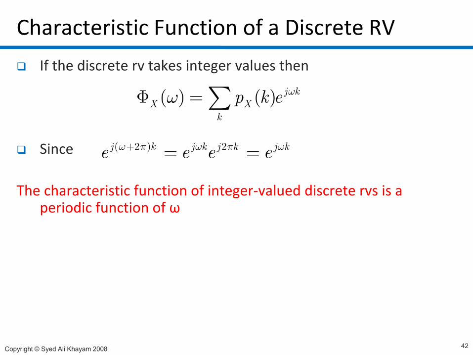
If the discrete rv takes integer values then
( ) ( ) j kX Xp k e
ωωΦ =∑
Since
( ) ( )X Xk
p k eωΦ ∑( 2 ) 2j k j k j k j ke e e eω π ω π ω+ = =Since
The characteristic function of integer-valued discrete rvs is a i di f i f
( )e e e e= =
periodic function of ω
Copyright © Syed Ali Khayam 2008 42
Characteristic Function of a Discrete RV
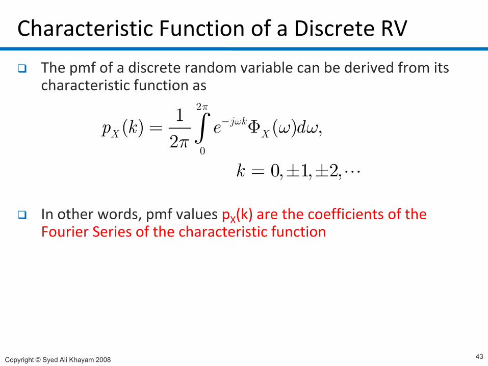
The pmf of a discrete random variable can be derived from its characteristic function as
22
0
1( ) ( ) ,2
j kX Xp k e d
πω ω ω
π−= Φ∫
I h d f l (k) h ffi i f h
0, 1, 2,k = ± ±
In other words, pmf values pX(k) are the coefficients of the Fourier Series of the characteristic function
Copyright © Syed Ali Khayam 2008 43
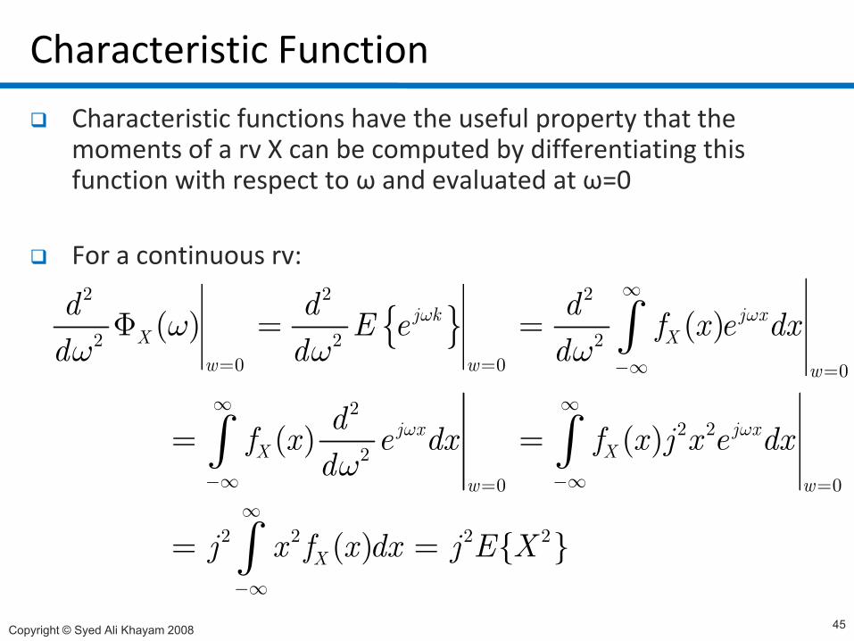
Characteristic Function
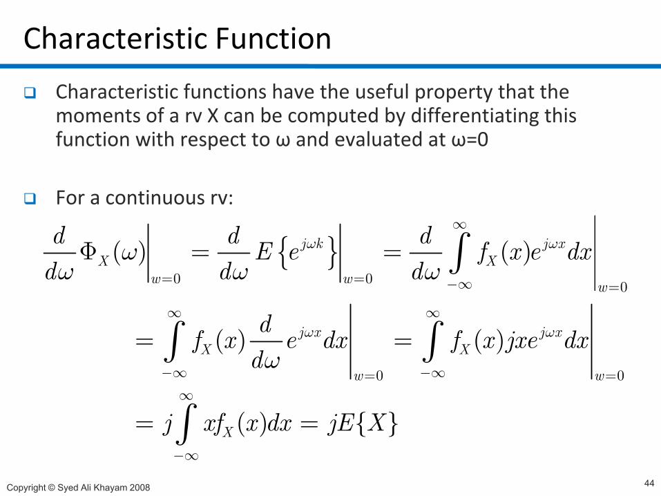
Characteristic functions have the useful property that the moments of a rv X can be computed by differentiating this function with respect to ω and evaluated at ω=0function with respect to ω and evaluated at ω=0
For a continuous rv:
{ }0 0 0
( ) ( )j k j xX X
w w
d d dE e f x e dxd d d
ω ωωω ω ω
∞
= = ∞
Φ = = ∫0 0 0
( ) ( )
w
j x j xX X
df x e dx f x jxe dxd
ω ω
−∞ =
∞ ∞
= =∫ ∫0 0
( ) ( )
( ) { }
w wd
j xf x dx jE X
ω−∞ −∞= =∞
= =
∫ ∫
∫Copyright © Syed Ali Khayam 2008 44
( ) { }Xj xf x dx jE X−∞
= =∫
Characteristic Function
Characteristic functions have the useful property that the moments of a rv X can be computed by differentiating this function with respect to ω and evaluated at ω=0function with respect to ω and evaluated at ω=0
For a continuous rv:
{ }2 2 2
2 2 20 0 0
( ) ( )j k j xX X
w w
d d dE e f x e dxd d d
ω ωωω ω ω
∞
= = ∞
Φ = = ∫0 0 0
22 2
2( ) ( )
w w w
j x j xX X
df x e dx f x j x e dxd
ω ω
= = −∞ =
∞ ∞
= =∫ ∫2
0 0
2 2 2 2
( ) ( )
( ) { }
w wd
j x f x dx j E X
ω−∞ −∞= =∞
= =
∫ ∫
∫Copyright © Syed Ali Khayam 2008 45
( ) { }Xj x f x dx j E X−∞
= =∫
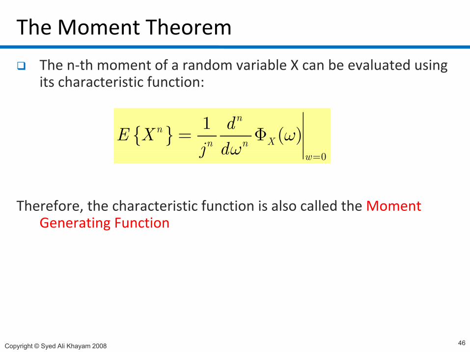
The Moment Theorem
The n-th moment of a random variable X can be evaluated using its characteristic function:
{ } 1 ( )n
nXn n
dE Xj d
ωω
= Φ
Th f h h i i f i i l ll d h M
0wj dω =
Therefore, the characteristic function is also called the Moment Generating Function
Copyright © Syed Ali Khayam 2008 46
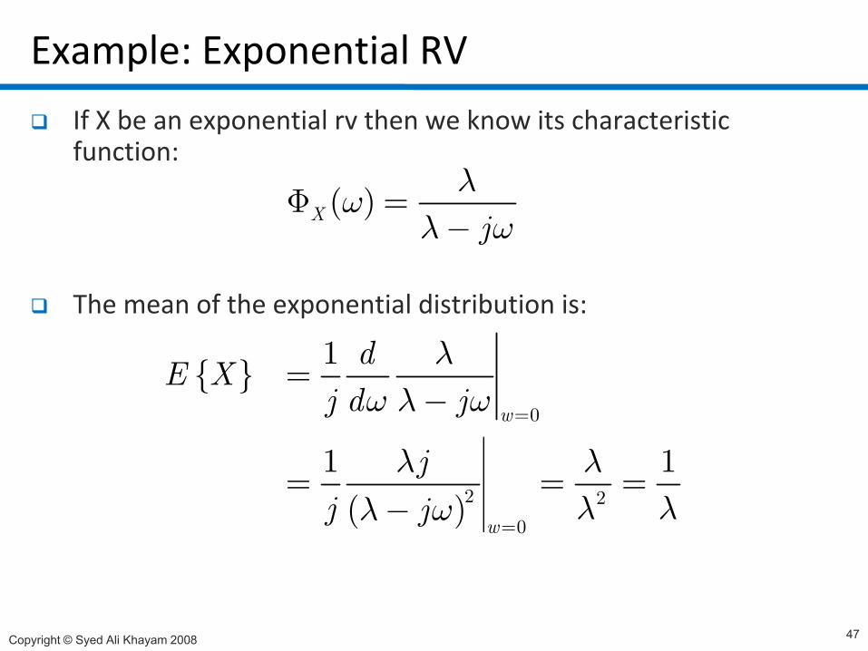
Example: Exponential RV
If X be an exponential rv then we know its characteristic function:
λ( )X jλω
λ ωΦ =
−
The mean of the exponential distribution is:
{ } 1 dE X λ{ }0
1 1w
E Xj d j
j
ω λ ω
λ λ=
=−
( )2 20
1 1
w
jj j
λ λλ λλ ω
=
= = =−
Copyright © Syed Ali Khayam 2008 47
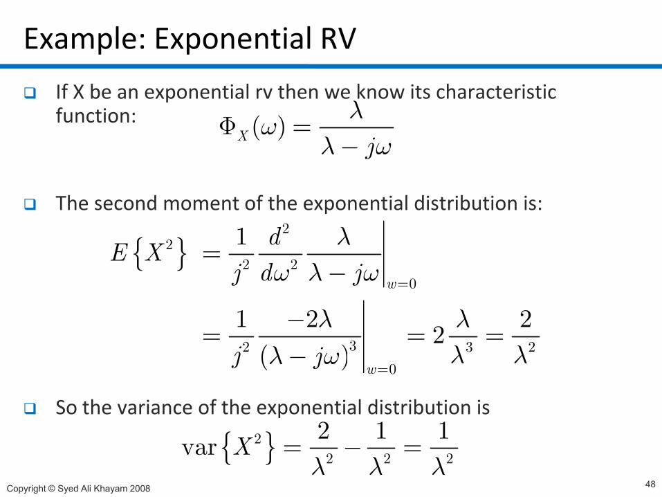
Example: Exponential RV
If X be an exponential rv then we know its characteristic function: ( )X j
λωλ
Φ =
The second moment of the exponential distribution is:
jλ ω−
p
{ }2
22 2
0
1
w
dE Xj d j
λω λ ω =
=−
( )
0
32 3 2
1 2 22
wj j
j jλ λ
λ λλ ω
=
−= = =
So the variance of the exponential distribution is
( )0w
j j λ λλ ω=
−
2 1 1
Copyright © Syed Ali Khayam 2008 48
{ }2 2 2 2
2 1 1var Xλ λ λ
= − =
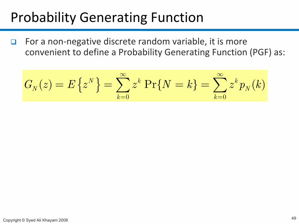
Probability Generating Function
For a non-negative discrete random variable, it is more convenient to define a Probability Generating Function (PGF) as:
{ }0 0
( ) Pr{ } ( )N k kN N
k k
G z E z z N k z p k∞ ∞
= = = =∑ ∑0 0k k= =
Copyright © Syed Ali Khayam 2008 49
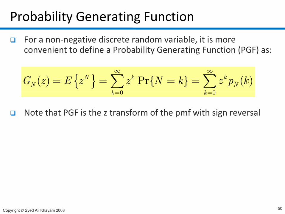
Probability Generating Function
For a non-negative discrete random variable, it is more convenient to define a Probability Generating Function (PGF) as:
{ }0 0
( ) Pr{ } ( )N k kN N
k k
G z E z z N k z p k∞ ∞
= = = =∑ ∑
Note that PGF is the z transform of the pmf with sign reversal
0 0k k= =
Copyright © Syed Ali Khayam 2008 50
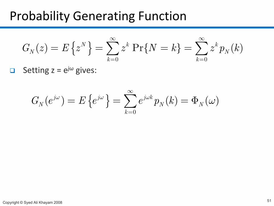
Probability Generating Function
{ }0 0
( ) Pr{ } ( )N k kN N
k k
G z E z z N k z p k∞ ∞
= = = =∑ ∑Setting z = ejω gives:
0 0k k= =
{ }0
( ) ( ) ( )j j j kN N N
k
G e E e e p kω ω ω ω∞
=
= = = Φ∑
Copyright © Syed Ali Khayam 2008 51
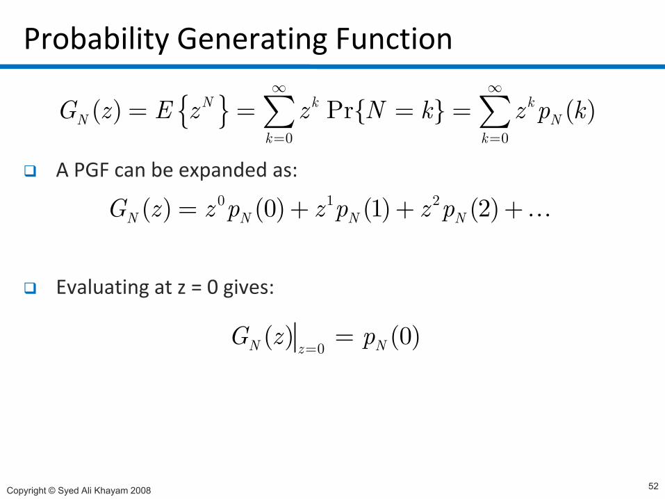
Probability Generating Function
{ }0 0
( ) Pr{ } ( )N k kN N
k k
G z E z z N k z p k∞ ∞
= =
= = = =∑ ∑A PGF can be expanded as:
0 0k k
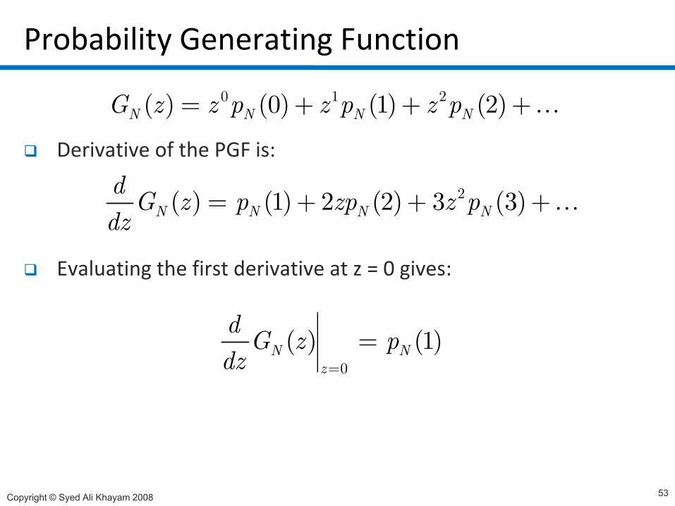
0 1 2( ) (0) (1) (2)N N N NG z z p z p z p= + + +…
Evaluating at z = 0 gives:
( ) (0) (1) (2)N N N NG z z p z p z p+ + +…
Evaluating at z = 0 gives:
0( ) (0)N Nz
G z p= =
Copyright © Syed Ali Khayam 2008 52
Probability Generating Function
D i ti f th PGF i
0 1 2( ) (0) (1) (2)N N N NG z z p z p z p= + + +…
Derivative of the PGF is:
2( ) (1) 2 (2) 3 (3)N N N Nd G z p zp z pd
= + + +…
Evaluating the first derivative at z = 0 gives:
dz
( ) (1)N Nd G z pdz
=0zdz =
Copyright © Syed Ali Khayam 2008 53
Probability Generating Function
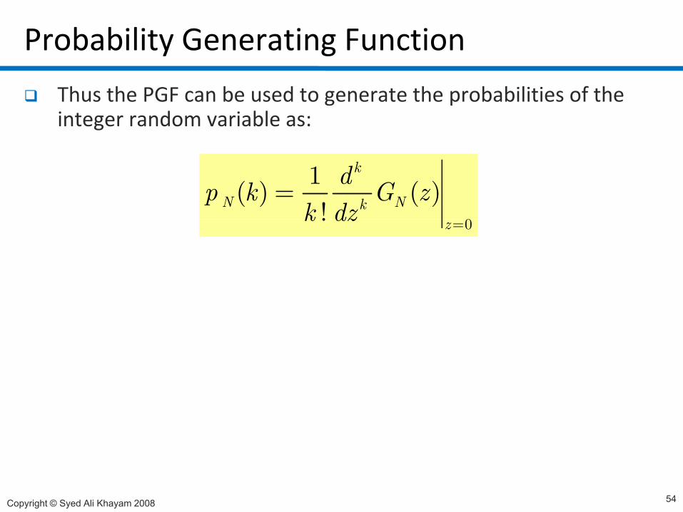
Thus the PGF can be used to generate the probabilities of the integer random variable as:
0
1( ) ( )!
k
N Nk
dp k G zk dz
=0! zk dz =
Copyright © Syed Ali Khayam 2008 54
Probability Generating Function
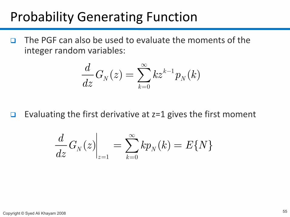
The PGF can also be used to evaluate the moments of the integer random variables:
1
0
( ) ( )kN N
k
d G z kz p kdz
∞−
=
=∑
Evaluating the first derivative at z=1 gives the first moment
1 0
( ) ( ) { }N Nk
d G z kp k E Ndz
∞
= =∑1 0z kdz = =
Copyright © Syed Ali Khayam 2008 55
Probability Generating Function
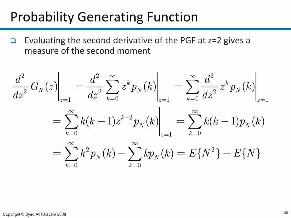
Evaluating the second derivative of the PGF at z=2 gives a measure of the second moment
2 2 2
2 2 2( ) ( ) ( )k kN N N
d d dG z z p k z p kd d d
∞ ∞
= =∑ ∑0 01 1 1
2( 1) ( ) ( 1) ( )
k kz z z
kN N
dz dz dz
k k z p k k k p k
= == = =
∞ ∞−= − = −
∑ ∑
∑ ∑0 01
2 2
( ) ( ) ( ) ( )
( ) ( ) { } { }
N Nk kz
N N
p p
k p k kp k E N E N
= ==∞ ∞
= − = −
∑ ∑
∑ ∑0 0
( ) ( ) { } { }N Nk k
k p k kp k E N E N= =∑ ∑
Copyright © Syed Ali Khayam 2008 56
Example: Poisson Random Variable
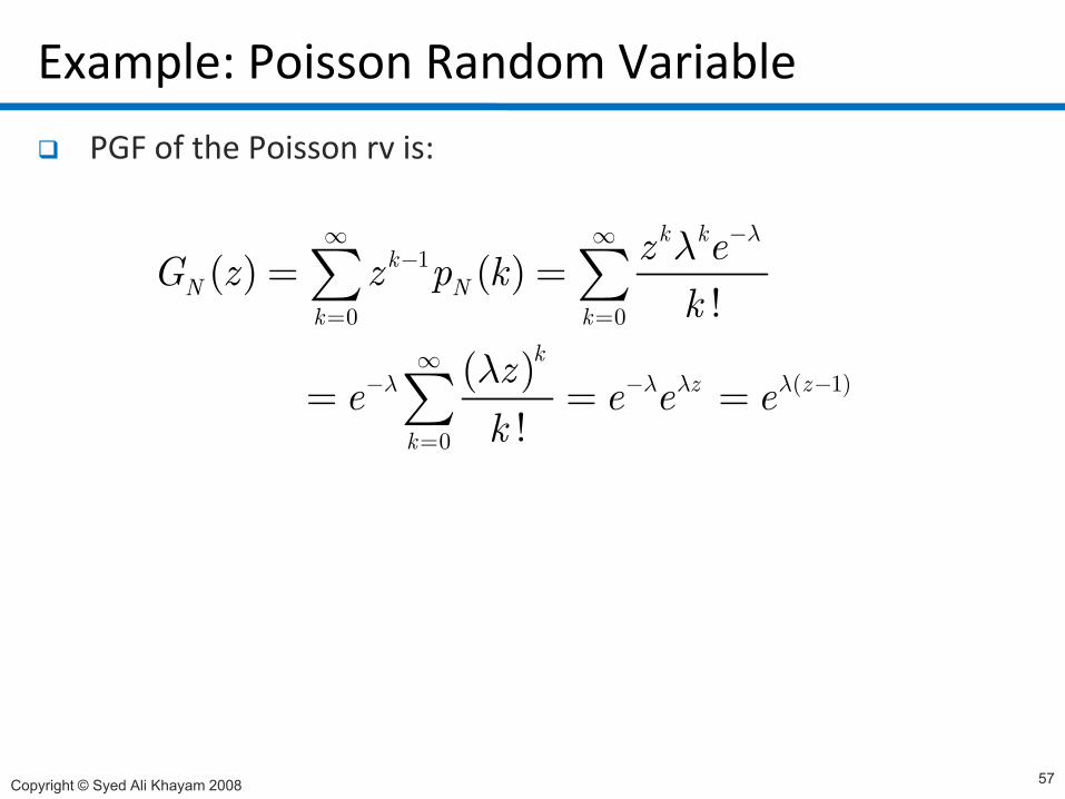
PGF of the Poisson rv is:
k k λ1
0 0
( ) ( )!
k kk
N Nk k
z eG z z p kk
λλ −∞ ∞−
= =
= =∑ ∑( ) ( 1)
0 !
kz z
k
ze e e e
kλ λ λ λλ∞
− − −
=
= = =∑
Copyright © Syed Ali Khayam 2008 57
Example: Poisson Random Variable
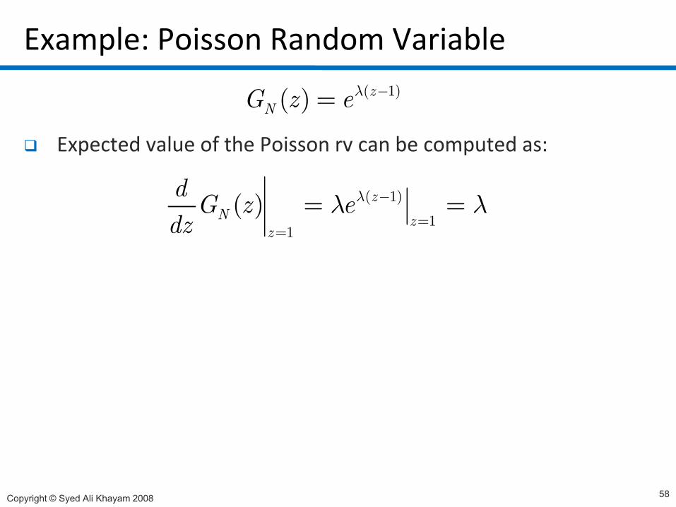
Expected value of the Poisson rv can be computed as:
( 1)( ) zNG z eλ −=
Expected value of the Poisson rv can be computed as:
( 1)
1( ) z
Nd G z ed
λλ λ−= =1
1
( )N zzdz ==
Copyright © Syed Ali Khayam 2008 58
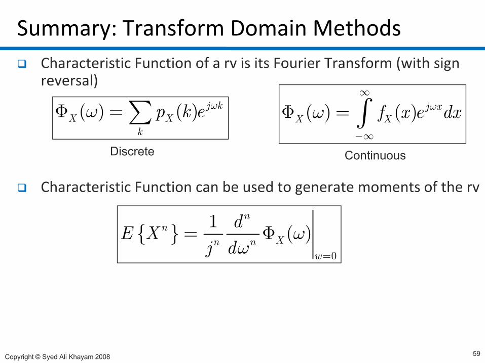
Summary: Transform Domain MethodsCharacteristic Function of a rv is its Fourier Transform (with sign reversal)
j∞
∫( ) ( ) j k∑ ( ) ( ) j xX Xf x e dx
ωω−∞
Φ = ∫( ) ( ) j kX X
k
p k e ωωΦ =∑Discrete Continuous
Characteristic Function can be used to generate moments of the rv
sc e e Continuous
{ }0
1 ( )n
nXn n
w
dE Xj d
ωω =
= Φ0w
Copyright © Syed Ali Khayam 2008 59
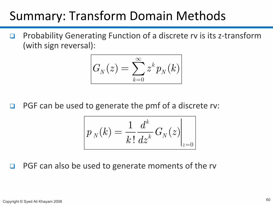
Summary: Transform Domain MethodsProbability Generating Function of a discrete rv is its z-transform (with sign reversal):
∞
0
( ) ( )kN N
k
G z z p k∞
=
=∑
PGF can be used to generate the pmf of a discrete rv:
0
1( ) ( )!
k
N Nkz
dp k G zk dz =
=
PGF can also be used to generate moments of the rv
0z
Copyright © Syed Ali Khayam 2008 60
HomeworkDerive the characteristic function of the Gaussian Random Variable
Textbook Problems3.923.100
Copyright © Syed Ali Khayam 2008 61
Related Documents