CS 355 NOTES - math.purdue.edu

CS 355 NOTES

ARUN DEBRAY

MAY 15, 2014

Contents

1. Pseudorandomness and the Blum-Micali generator: 4/1/14 12. Proof of Security of the Blum-Micali Generator: 4/3/14 43. The Goldreich-Levin Theorem: 4/8/14 64. Commitments: 4/10/14 95. Commitments II: 4/17/14 126. Oblivious Transfer: 4/22/14 147. Oblivious Transfer II: 4/24/14 168. Zero-Knowledge Proofs: 4/29/14 1810. Zero-Knowledge Proofs III: 5/6/14 2111. Zero-Knowledge Proofs IV: 5/8/14 2212. Elliptic Curves: 5/13/14 2513. Elliptic Curves and Pairings: 5/15/14 27

1. Pseudorandomness and the Blum-Micali generator: 4/1/14

“This room is really hot. I’m going to come next time in my bathing suit, I think.”

There will be three homework assignments in this class (though that sometimes means two, the professor will try tomake three this quarter). Please submit them electronically. There are no exams.

The course website is http://crypto.stanford.edu/~dabo/cs355/; this contains all of the relevant papers aswell as the draft of a textbook (which is password-protected).

We will start with pseudorandomness, which is a foundation and important concept within crypto, but also a good,gentle way to introduce crypto-style proofs.

The first thing we’ll do is introduce some notation from crypto and discrete probability, to make sure we’re all onthe same page.

Definition.

• A probability space (Ω,Pr) is a tuple where Ω is a set (which in this class will always be finite) andPr : 2Ω → [0, 1] such that Pr[Ω] = 1 and for all sets F ⊆ Ω, the probability of F can be defined as

Pr[F ] =∑x∈F

Pr[x].

F is called an event, and is said to happen with probability Pr[A].• Two events A and B are independent if Pr[A ∩B] = Pr[A] · Pr[B].

Definition. There are two kinds of random variables:

• A Type I random variable is a function X : Ω→ S, for a finite set S. For a predicate Q : S → 0, 1, we candefine

Pr[Q(X)] =∑y∈Ω

Pr[y].

For example, we could have a random variable that, on the probability space of strings of a given length,returns the sum of their bits, and the predicate could be whether they are even.

– The notation XR← Ω means that X is a uniform random variable on Ω.

1

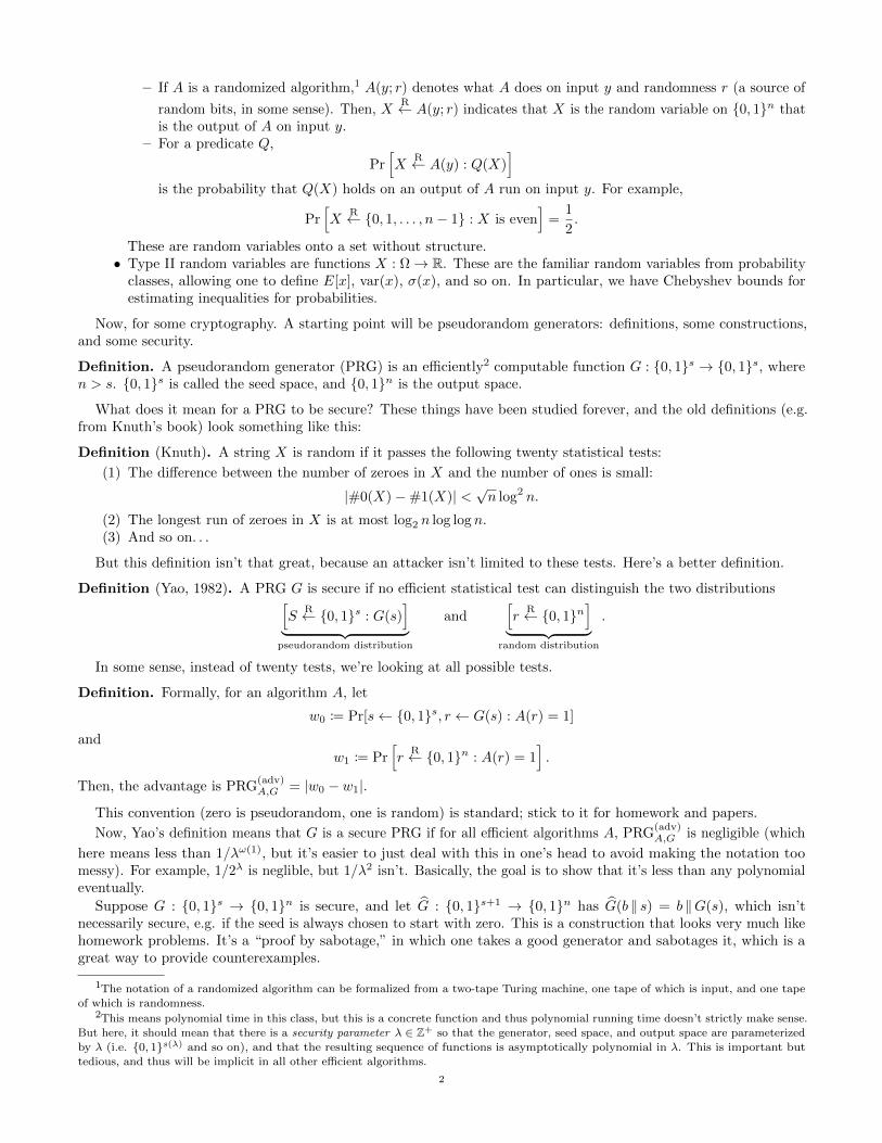
– If A is a randomized algorithm,1 A(y; r) denotes what A does on input y and randomness r (a source of

random bits, in some sense). Then, XR← A(y; r) indicates that X is the random variable on 0, 1n that

is the output of A on input y.– For a predicate Q,

Pr[X

R← A(y) : Q(X)]

is the probability that Q(X) holds on an output of A run on input y. For example,

Pr[X

R← 0, 1, . . . , n− 1 : X is even]

=1

2.

These are random variables onto a set without structure.• Type II random variables are functions X : Ω→ R. These are the familiar random variables from probability

classes, allowing one to define E[x], var(x), σ(x), and so on. In particular, we have Chebyshev bounds forestimating inequalities for probabilities.

Now, for some cryptography. A starting point will be pseudorandom generators: definitions, some constructions,and some security.

Definition. A pseudorandom generator (PRG) is an efficiently2 computable function G : 0, 1s → 0, 1s, wheren > s. 0, 1s is called the seed space, and 0, 1n is the output space.

What does it mean for a PRG to be secure? These things have been studied forever, and the old definitions (e.g.from Knuth’s book) look something like this:

Definition (Knuth). A string X is random if it passes the following twenty statistical tests:

(1) The difference between the number of zeroes in X and the number of ones is small:

|#0(X)−#1(X)| <√n log2 n.

(2) The longest run of zeroes in X is at most log2 n log log n.(3) And so on. . .

But this definition isn’t that great, because an attacker isn’t limited to these tests. Here’s a better definition.

Definition (Yao, 1982). A PRG G is secure if no efficient statistical test can distinguish the two distributions[S

R← 0, 1s : G(s)]

︸ ︷︷ ︸pseudorandom distribution

and[r

R← 0, 1n]

︸ ︷︷ ︸random distribution

.

In some sense, instead of twenty tests, we’re looking at all possible tests.

Definition. Formally, for an algorithm A, let

w0 := Pr[s← 0, 1s, r ← G(s) : A(r) = 1]

and

w1 := Pr[r

R← 0, 1n : A(r) = 1].

Then, the advantage is PRG(adv)A,G = |w0 − w1|.

This convention (zero is pseudorandom, one is random) is standard; stick to it for homework and papers.

Now, Yao’s definition means that G is a secure PRG if for all efficient algorithms A, PRG(adv)A,G is negligible (which

here means less than 1/λω(1), but it’s easier to just deal with this in one’s head to avoid making the notation toomessy). For example, 1/2λ is neglible, but 1/λ2 isn’t. Basically, the goal is to show that it’s less than any polynomialeventually.

Suppose G : 0, 1s → 0, 1n is secure, and let G : 0, 1s+1 → 0, 1n has G(b ‖ s) = b ‖G(s), which isn’tnecessarily secure, e.g. if the seed is always chosen to start with zero. This is a construction that looks very much likehomework problems. It’s a “proof by sabotage,” in which one takes a good generator and sabotages it, which is agreat way to provide counterexamples.

1The notation of a randomized algorithm can be formalized from a two-tape Turing machine, one tape of which is input, and one tape

of which is randomness.2This means polynomial time in this class, but this is a concrete function and thus polynomial running time doesn’t strictly make sense.

But here, it should mean that there is a security parameter λ ∈ Z+ so that the generator, seed space, and output space are parameterizedby λ (i.e. 0, 1s(λ) and so on), and that the resulting sequence of functions is asymptotically polynomial in λ. This is important but

tedious, and thus will be implicit in all other efficient algorithms.

2

Note at this point that we can’t prove that any PRGs exist; in fact, to prove that something is a PRG would implythat P 6= NP, and conversely. That would be neat, but we probably won’t get to it in this course.

Definition. A one-bit PRG is a secure PRG G : 0, 1s → 0, 1s+1.

Today we’re going to assume that one-bit PRGs exist. (It’s a nice theorem that the existence of one-waypermutations exist implies the existence of one-bit PRGs, but that’s a story for next lecture.) Then, we want toproduce a secure PRG GBM that takes a one-bit PRG and expands it into a many-bit PRG, using a constructioncalled the Blum-Micali generator.

We’ll generalize the notation to G : S → R× S, where S is the seed space. For a one-bit PRG, S = 0, 1s andR = 0, 1. Then, the goal is to produce a secure PRG GBM : S → Rn × S for any n > 0.

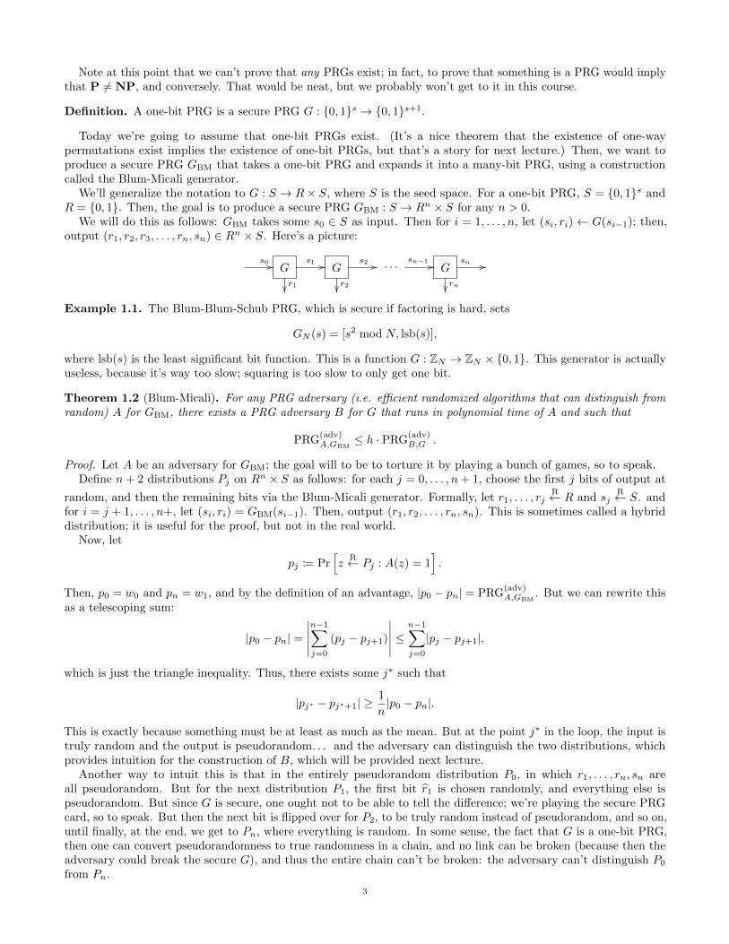
We will do this as follows: GBM takes some s0 ∈ S as input. Then for i = 1, . . . , n, let (si, ri)← G(si−1); then,output (r1, r2, r3, . . . , rn, sn) ∈ Rn × S. Here’s a picture:

s0 // Gr1

s1 // Gs2 //

r2

· · ·sn−1 // G

rn

sn //

Example 1.1. The Blum-Blum-Schub PRG, which is secure if factoring is hard, sets

GN (s) = [s2 mod N, lsb(s)],

where lsb(s) is the least significant bit function. This is a function G : ZN → ZN × 0, 1. This generator is actuallyuseless, because it’s way too slow; squaring is too slow to only get one bit.

Theorem 1.2 (Blum-Micali). For any PRG adversary (i.e. efficient randomized algorithms that can distinguish fromrandom) A for GBM, there exists a PRG adversary B for G that runs in polynomial time of A and such that

PRG(adv)A,GBM

≤ h · PRG(adv)B,G .

Proof. Let A be an adversary for GBM; the goal will to be to torture it by playing a bunch of games, so to speak.Define n+ 2 distributions Pj on Rn × S as follows: for each j = 0, . . . , n+ 1, choose the first j bits of output at

random, and then the remaining bits via the Blum-Micali generator. Formally, let r1, . . . , rjR← R and sj

R← S. andfor i = j + 1, . . . , n+, let (si, ri) = GBM(si−1). Then, output (r1, r2, . . . , rn, sn). This is sometimes called a hybriddistribution; it is useful for the proof, but not in the real world.

Now, let

pj := Pr[z

R← Pj : A(z) = 1].

Then, p0 = w0 and pn = w1, and by the definition of an advantage, |p0 − pn| = PRG(adv)A,GBM

. But we can rewrite thisas a telescoping sum:

|p0 − pn| =

∣∣∣∣∣n−1∑j=0

(pj − pj+1)

∣∣∣∣∣ ≤n−1∑j=0

|pj − pj+1|,

which is just the triangle inequality. Thus, there exists some j∗ such that

|pj∗ − pj∗+1| ≥1

n|p0 − pn|.

This is exactly because something must be at least as much as the mean. But at the point j∗ in the loop, the input istruly random and the output is pseudorandom. . . and the adversary can distinguish the two distributions, whichprovides intuition for the construction of B, which will be provided next lecture.

Another way to intuit this is that in the entirely pseudorandom distribution P0, in which r1, . . . , rn, sn areall pseudorandom. But for the next distribution P1, the first bit r1 is chosen randomly, and everything else ispseudorandom. But since G is secure, one ought not to be able to tell the difference; we’re playing the secure PRGcard, so to speak. But then the next bit is flipped over for P2, to be truly random instead of pseudorandom, and so on,until finally, at the end, we get to Pn, where everything is random. In some sense, the fact that G is a one-bit PRG,then one can convert pseudorandomness to true randomness in a chain, and no link can be broken (because then theadversary could break the secure G), and thus the entire chain can’t be broken: the adversary can’t distinguish P0

from Pn.

3

2. Proof of Security of the Blum-Micali Generator: 4/3/14

“So first, I’m impressed that you all came back. Congratulations.”

The first thing we need to do is provide a full proof of Theorem 1.2, rather than just intuition, but we can alsogeneralize it slightly.

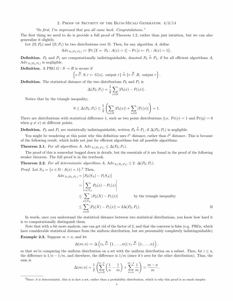
Let (Ω, P0) and (Ω, P1) be two distributions over Ω. Then, for any algorithm A, define

AdvA,(P0,P1) := |Pr [X ← P0 : A(x) = 1]− Pr [x← P1 : A(x) = 1]| .

Definition. P0 and P1 are computationally indistinguishable, denoted P0c≈ P1, if for all efficient algorithms A,

AdvA,(P0,P1) is negligible.

Definition. A PRG G : S → R is secure ifs

R← S, r ← G(s), output rc≈ r R← R, output r

.

Definition. The statistical distance of the two distributions P0 and P1 is

∆(P0;P1) =1

2

∑x∈Ω

|P0(x)− P1(x)| .

Notice that by the triangle inequality,

0 ≤ ∆(P0;P1) ≤ 1

2

(∑x∈Ω

|P0(x)|+∑x∈Ω

|P1(x)|

)= 1.

There are distributions with statistical difference 1, such as two point distributions (i.e. Pr(x) = 1 and Pr(y) = 0when y 6= x) at different points.

Definition. P0 and P1 are statistically indistinguishable, written P0s≈ P1, if ∆(P0;P1) is negligible.

You might be wondering at this point why this definition uses `1 distance, rather than `2 distance. This is becauseof the following result, which holds not just for efficient algorithms but all possible algorithms.

Theorem 2.1. For all algorithms A, AdvA,(P0,P1) ≤ ∆(P0;P1).

The proof of this is somewhat bogged down in details, but the essentials of it are found in the proof of the followingweaker theorem. The full proof is in the textbook.

Theorem 2.2. For all deterministic algorithms A, AdvA,(P0,P1) ≤ 2 ·∆(P0;P1).

Proof. Let SA = x ∈ Ω : A(x) = 1.3 Then,

AdvA,(P0,P1) =∣∣P0(SA)− P(SA)

∣∣=

∣∣∣∣∣ ∑x∈SA

P0(x)− P1(x)

∣∣∣∣∣≤∑x∈SA

|P0(X)− P1(x)| by the triangle inequality

≤∑x∈Ω

|P0(X)− P1(x)| = 2∆(P0;P1).

In words, once you understand the statistical distance between two statistical distributions, you know how hard itis to computationally distinguish them.

Note that with a bit more analysis, one can get rid of the factor of 2, and that the converse is false (e.g. PRGs, whichhave considerable statistical distance from the uniform distribution, but are presumably completely indistinguishable).

Example 2.3. Suppose m > n, and let

∆(m;n) := ∆(r0

R← 1, . . . ,m; r1R← 1, . . . , n

),

so that we’re comparing the uniform distribution on a set with the uniform distribution on a subset. Then, for i ≤ n,the difference is 1/n− 1/m, and elsewhere, the difference is 1/m (since it’s zero for the other distribution). Thus, thesum is

∆(m;n) =1

2

(n−1∑x=0

(1

n− 1

m

)+

m−1∑x=n

1

m

)=m− nm

.

3Since A is deterministic, this is in fact a set, rather than a probability distribution, which is why this proof is so much simpler.

4

Remember this calculation; it’s a very important fact in crypto. Notice that this means that when m is close to n,then the two distributions are indistinguishable, especially when n is large. This is a good way to bridge gaps inproofs (e.g. if you can only show something is secure on a very slightly smaller distribution).

For an application, suppose we’re given a secure PRG G : S → 0, . . . , 2` − 1, and want to construct aG′ : S → 0, 1, . . . , n− 1, where n < 2`.4 Define G′(s) = G(s) mod n. Under what conditions is G′ secure?

Theorem 2.4. For all adversaries A for G′, there exists an adversary B for G such that

Adv(PRG)A,G′ ≤ Adv

(PRG)B,G +

n

2`,

and such that B runs in about the same running time as A.

Thus, for G′ to be secure, we need n/2` to be negligible. In practical terms, this means it should be less than1/2128, so ` ≈ log2 n+ 128.

Proof of Theorem 2.4. First, for notation, define m = 2` and k = bm/nc, so that 0 < m− k/n < n.Then, given an algorithm A attacking G′, construct an algorithm B which, on input x ∈ 0, . . . ,m− 1 outputs

A(x mod n). So why does this break G? Let

p0 := Pr[s

R← S, r ← G(S) mod n : A(r) = 1]

= Pr[s

R← S, r ← G(s) : B(r) = 1],

which is just notation-chasing. And the second term of the advantage is

p1 := Pr[r

R← 0, . . . , n− 1 : A(r) = 1]

= Pr[r

R← 0, . . . , k · n− 1 : A(r mod n) = 1]

= Pr[r

R← 0, . . . , kn− 1 : B(r) = 1].

But this isn’t yet in terms of the advantage of B, because it wasn’t in terms of the distribution on 0, . . . , kn− 1.Instead, we can introduce an intermediate distribution which has the probabilities we like. This is a common trick inthese sorts of proofs. Thus, let

p∗ = Pr[r

R← 0, . . . , n− 1 : B(r) = 1].

Now, we can once again use the triangle inequality:

Adv(PRG)A,G′ = |p1 − p0| = |p1 − p∗ + p∗ − p0|

≤ |p1 − p∗|+ |p∗ − p0|

≤ m− knm

+ Adv(PRG)B,G

≤ n

m+ Adv

(PRG)B,G .

This proof might look somewhat complicated, but it’s in some sense trivial; the only trick is to introduce the newdistribution, and then use the statistical distance. This sort of proof is sometimes known as a hybrid argument.

Now, back to the Blum-Micali generator, and specifically the proof that the construction is secure (in a specificsense mentioned in the theorem statement).

Proof of Theorem 1.2. Let A be a PRG adversary for GBM, and our goal is to build an algorithm B that breaks G.Furthermore, use the notation that r is random and r is pseudorandom for bits r.

For j = 0, . . . , n, pet pj be the following hybrid distribution: let r1, . . . , rjR← R and sj

R← S, and then fori = j + 1, . . . , n, let (ri, si)← G(Si−1). Then, output (r1, . . . , rj , rj+1, . . . , rn, sn). Thus, p0 is entirely pseudorandom

and pn is totally random, and if pj := Pr [z ← Pj : A(z) = 1], then Adv(PRG)A,GBM

= |p0 − pn|.The goal is to show that P0

c≈ P1

c≈ · · ·

c≈ Pn, and thus that P0

c≈ Pn (since it’s an equivalence relation).5

The general idea is illustrated by arguing that A can’t distinguish Pj and Pj+1: specifically, that there exists a Bj

such that |pj − pj−1| = Adv(PRG)Bj ,G

, which is negligible. In other words, if this algorithm is non-negligible, then Bj can

break G.Specifically, on input (r∗, s∗) ∈ R×S, Bj does the following: it generates random bits r1, . . . , rj ∈ R and sets sj+1 :

= s∗. Then, for i = j + 2, . . . , n, let (ri, si)← G(si−1), and output A(z), where z = (r1, . . . , rj , r∗, rj+2, . . . , rn, sn).

4One place this appears is Diffie-Hellman, since the order of the group is prime and therefore not a power of 2.5This is a common enough technique that for experts in crypto, this would be the end of the proof.

5

if (r∗, s∗)R← S, then z

R← Pj+1, because the first j + 1 bits of z are truly random, and the remaining bits arepseudorandom, which is exactly what Pj+1 is. Thus,

Pr[(r∗, s∗)

R← R× S : B(r∗, s∗) = 1]

= pj+1.

In the second case, where (r∗, s∗)← G(s) where sR← S, then z

R← Pj , because the first j bits are truly random, andthe remaining bits are pseudorandom. Thus,

Pr[s

R← S, (r∗, s∗a)← G(s) : B(r∗, s∗) = 1]

= pj .

Thus,

Adv(PRG)A,GBM

= |p0 − pn| = |p0 − p1 + p1 − p2 + · · ·+ Pn−1 − pn|

=

n−1∑i=0

|pi − pi+1|

=

n−1∑i=0

AdvBi,G .

But since G is secure, then each of these must be negligible, and therefore their sum is. Yet we have somethingslightly stronger to prove; if GBM is insecure, we don’t know yet which one of the Bi has non-negligible advantage,which is necessary to complete the proof.

So. . . have the algorithm B choose one of the Bi at random and run it. This breaks G with non-negligibleprobability, as AdvB,G = (1/n) ·AdvA,GBM . This involves writing some conditional probabilities, conditioning on j:

Pr[B = 1] =

n−1∑k=1

Pr[B = 1 | j = k] Pr[k] =

n−1∑k=1

Pr[Bj = 1]1

n,

and then the negligible terms go away.

This proof seems very tedious, but the point is that all of the details have been done once, and now the proofs inclass can be a little more streamlined, with the technical details left to the exercises.

Example 2.5. Blum-Micali generators occur in the real world:

• RC4 was recently declared dead (don’t use it!), but it’s still used by much of the world to encrypt Web traffic.The state of the generator is an array s of length 255, along with two pointers i and j into the array. Then,it outputs s[s[i] + s[j]], and then increments i by 1 and sets j ← j + s[i]. Then, swap s[i] and s[j]. This isviewed as a Blum-Micali generator in that it outputs something, and then a new state.

The specific issue with RC4 is that it leaks the first few bytes (which often are the authentication cookie,which is bad), so if you must use it, let it run for a little while before beginning encryption.• There is another Blum-Micali generator called Trivium.• A bad example, called LCG, the linear combinational generator. Fix a prime p, and a, b ∈ Zp. Then given

some seed s ∈ Zp, let LCG(s) = (lsb(s), as + b mod p). This is completely insecure, and admits a nicegeometrical attack involving lattices: given a few bits of the output (roughly log p), one can reconstruct theseed. Oops.

• Last time, we saw the BBS generator, which changes and fixes this to BBS(s) = (lsb(s), s2 mod N), which isas secure as factoring, where N = pq is an RSA modulus.

3. The Goldreich-Levin Theorem: 4/8/14

“It would be the joke of the century if Dan Bernstein turned out to be an agent of the NSA.”

Recall last week that we introduced the notion of computational indistinguishability of distributions, P0c≈ P1, and

that of statistical indistinguishability P0s≈ P1. Then, we defined a PRG G : S → R to be secure if s R← S : G(S)

c≈

r R← R : r. The Blum-Micali generator accepts PRGs:

G : S → R× S BM−→ GBM : S → Rn × S.

The GGM generator takes a generator that doubles the size of the seed (which can be constructed via Blum-

Micali or other means) G : S → S × S, and will produce a G(d)GGM : S → S(2d). In essence, given some s ∈ S,

G(1) : s 7→ G(s) = (s1, s2), then G(2) : s 7→ (G(s1), G(s2)), which has four elements, and so on.6

Theorem 3.1. If G is a secure PRG, then for any constant d, G(d)GGM is also a secure PRG. Specifically, for all

efficient adversaries A for G(d)GGM there exists an adversary B for G such that

Adv(PRG)

A,G(d)GGM

≤ 2d Adv(PRG)B,G .

Proof. Consider the tree of values produced by GBBM: s1 and s2 from some random s, s3, . . . , s6 from s1 and s2, andso on. But this is computationally indistinguishable from the case where s1 and s2 are chosen by random and pluggedinto the generator for s1 and s2 (for if it were distinguishable, then G wouldn’t be secure, as in the proof from lastlecture). But this is computationally indistinguishable from the case where s3, . . . , s6 are truly random rather thanpseudorandom, and so on.

It turns out one can strengthen this construction to produce a PRF.Of course, nobody uses this generator to actually construct stream ciphers. In the real world, there is exactly one

generator used in the real world, and that is counter mode (e.g. one called ChaCha, which is or will be used at Googleand was effectively pulled out of a hat by Dan Bernstein). This is based on a PRP.

One cute application of PRGs is to derandomize randomized algorithms. This is related to the major open problemin complexity theory as to whether BPP ⊆ P. This almost comes for free with the existence of secure PRGs. KetA(x; r) be a randomized efficient algorithm for some task (e.g. factoring, or graph coloring), and suppose that for allx ∈ I (where I is the input space):

Pr[x

R← R : A(x; r) = “success”]≥ 1

3,

i.e. for at least a third of the r, A finds a solution to the problem x. The power of randomness is that we know thereare many needles in the haystack that work (depending on x, of course), but we don’t know ahead of time which oneswork, and have to try them.

Let G : S → R be a secure PRG. Then, introduce a deterministic algorithm B(x) that, for all s ∈ S, tries A(x;G(s)),and outputs G(s) if the result is successful, and fails if none succeed. This has running time time(B) = time(A)× |S|(where G is assumed to be efficient), so as long as the size of the seed space is polynomial in that of x, then B is alsopolynomial-time if A is. Constructions like this are a good reason to keep seed spaces small.

Claim. If G is a secure PRG, then for all x ∈ I, B(x) will never fail.

Proof. Suppose there is an x ∈ I that makes B fail. This introduces a distinguisher D for G, which breaks the securegenerator. D works as follows: given some r ∈ R,

D(r) =

“random,” if A(x; r) = “success”“pseudorandom,” otherwise.

Thus,

Adv(PRG)D,G ≥ 1

3− 0 =

1

3,

(the latter because when x is bad, D never claims it to be pseudorandom), which is certainly non-negligible.

Notice that this proof depends on x being given to D from somewhere.Now, this is not a proof that BPP ⊆ P; we currently don’t know how to prove the existence of a secure PRG

(which also forces P 6= NP — so this proof isn’t a great way to approach the complexity theory, but it’s still prettyneat). Since we don’t have polynomial-time PRGs, then one might use a partial result, e.g. a PRG that is secureagainst log-space algorithms, which are weaker.6 So this proof works absolutely in this restricted case.

The Goldreich-Levin Theorem. This theorem is a classic result in crypto, allowing one to build PRGs fromweaker assumptions.

Definition.

(1) A one-to-one function f : X → X is called a one-way permutation if:• f is efficiently computable, and

• for all efficient adversaries A for f , Pr[x

R← X : A(f(x)) = x]

is negligible, i.e. f is “hard to invert.”

(2) A function f : X → Y is called a one-way function if:• f is efficiently computable, and

• for all efficient algorithms A for f , Pr[x

R← X : f(A(f(x))) = f(x)]

is negligible.

6Log-space, or L, is a class of deterministic algorithms that are restricted to space logarithmic in the size of the input. L ⊆ P.

7

Examples include cryptographic hash functions, such as SHA-256, f(x) = AES(x, 0), and so on. RSA is an exampleof a one-way permutation (which is slow and has lots of structure, and therefore isn’t the best first example). Bycontrast, one-way permutations are easy to construct: we know of no fast one-way permutations. There are some fromalgebra, though, such as f : 1, . . . , p − 1 → 1, . . . , p − 1 defined as f(x) = gx mod p (which is mathematicallyugly, in that it conflates multiplication and addition, but a bijection anyways). RSA is a bit of a problem, because itdepends on who knows the factorization; it can be formalized to be an OWP, however.

Even though one-way permutation are hard to construct, much of the theory of building PRGs depends on them.

Theorem 3.2 (Goldreich-Levin). Given a one-way permutation f , one can build a secure PRG.

Then, one can use the PRG to build a PRF and therefore a PRP. There is a construction going from OWFs toPRGs, but it’s much, much more complicated. The theoretical result is nice, but this theorem will find lots of otheruses in this course.

Interestingly, in practice it often goes the other way: one tends to start with a PRP, and then use counter mode tobuild a PRG, or the switching lemma to build a PRF.

Definition. Suppose f : X → Y is a one-way function. Then, another function h : X → R is said to be hardcore forf if

xR← X : (f(x), h(x))

c≈x

R← X, rR← R : (f(x), r)

.

In other words, even if f(x) is already given, it’s still not possible for an adversary to distinguish h(x) from random.A typical example is when R = 0, 1, in which case h is also called a hardcore bit.

Theorem 3.3. Let p be prime, g ∈ Z∗p be of prime order q, and f : 1, . . . , p− 1 → Z∗p sending x 7→ gx. Then, if f

is a one-way function,7 then h(x) = lsb(x) is hardcore for f .

Here, lsb(x) denotes the least significant bit of x. Interestingly, the corresponding h′(x) = msb(x), the mostsignificant bit, is not hardcore.

In other words, even given exponentiation, it’s not possible to distinguish the least significant bit from random.The proof is quite nice: given a distinguisher for only the least significant bit from random allows one to recover theentire discrete log.

For another example, called the BBS hardcore bit, one has the following theorem.

Theorem 3.4. Suppose N = pq for large primes p and q, and let f : ZN → ZN send x 7→ xe for some RSA constante 6= 2.8 Then, if f is a one-way permutation, then h(x) = lsb(x) is a hardcore bit for f .

Lemma 3.5. Suppose f : X → X is a one-way permutation and h : X → R is hardcore for f . Then, there exists asecure PRG G : X → X ×R given by G(s) = (f(s), h(s)).

Proof. Since h is hardcore, thens

R← X : (f(s), h(s))

c≈s

R← S, rR← R : (f(s), r)

s≈s

R← X, rR← R : (s, r)

,

the latter equivalence because f is a permutation: if one takes a random element of S and applies f , then the resultis another random element of S.

Notice that the last step implies that this construction doesn’t work for one-way functions. A typical counterexampleis, given a one-way function f , g(x) = [0 ‖ f(x)] is still a one-way function, but the construction given by the lemmaisn’t random.

Now, we can provide two constructions of hardcore bits. The first, the Goldreich-Levin method: supposef : 0, 1n → 0, 1n is an OWP, and define g : 0, 1n × 0, 1n → 0, 1n → 0, 1n as (x, r) 7→ (f(x), r). Then, thecontent of Theorem 3.2 is that if f is a one-way permutation, then the inner product

B(x, y) = 〈x, r〉 =

n∑i=1

xi · ri mod 2

is a hardcore bit for g. This is also known as the Goldreich-Levin bit.

7This is the discrete-log assumption, which is believed to be true but still technically open.8For example, one could choose e = 3 as long as 3 - ϕ(N).

8

Proof sketch for Theorem 3.2. Suppose B(x, r) isn’t hardcore for g. Then, there exists an efficient algorithm D suchthat

Pr [x, r → 0, 1n : D(g(x, r)) = B(x, r)] ≥ 1

2+ ε,

where ε is some non-negligible function. This follows from a few mechanical steps that involve expanding out thedefinition of a hardcore bit.

Let

S =

x | Pr

[r

R← 0, 1n : D(f(x), r) = 〈x, r〉]≥ 1

2+ε

2

.

Then, it’s a bit more mechanical work (some simple combinatorics) to show that |S| > (ε/2) · |X|.Now, fix an x ∈ S; then, D can be thought of as a function in just r. Specifically, there exists a D′ such that

Pr[r

R← 0, 1n : D′(r) = 〈r, x〉]≥ 1

2+ε

2.

Then, a result called the Goldreich-Levin algorithm (which will be presented next lecture) will show that D′ canrecover all such x with this property, even with this slight advantage. (It turns out there are at most O(1/ε2) such x.)

Suppose Pr[D′(r) = 〈r, x〉] = 1; then, it’s trivial to recover x (in some sense, an extreme case of the algorithm). Ifinstead Pr[D′(r) = 〈r, x〉] ≥ 3/4, then one can build a D′′(r) that is perfect in that it can recover x. This is a goodexercise; the general theorem is a little harder.

4. Commitments: 4/10/14

“One of the most important lessons of the Heartbleed bug is that if you ever in the future discover animportant exploit in a popular protocol, the first thing you must do is get a really cool logo.”

Recall that if f : X → X is a one-way permutation, then h : X → 0, 1 is a hardcore bit for f ifx

R← X : (f(x), h(x)

c≈x

R← X, bR← 0, 1 : (f(x), b)

,

or equivalently that for all efficient adversaries A,∣∣∣∣Pr[x

R← X : A(f(x)) = h(x)]− 1

2

∣∣∣∣is negligible.

We then defined the Goldreich-Levin bit: given a one-way permutation f : Zn2 → Zn2 , then we define g : Z2n2 → Z2n

2

by g(x, r) = (f(x), r). Then, Theorem 3.2 is that

h(x) = 〈x, r〉 =

n−1∑i=0

xi · ri mod 2

is hardcore for g.The key to this is not so much the theorem statement but the proof idea: if A is an algorithm such that

Pr [r ← Zn2 : A(r) = 〈x, r〉] > 1

2+ ε,

then there exists an algorithm B that can use A to output a list of o(1/e2) values (by running A on a bunch ofdifferent possible r), where x is one of the values. This is much easier to show when the 1/2 is replaced with 3/4.

This algorithm has applications throughout crypto, and even in learning theory and coding theory! A reinterpretationof the Goldreich-Levin algorithm for coding theory is as follows.

The Hadamard code is a set of code words in Zn2 : specifically, for every x ∈ Zn2 , we have a code word with length2n (i.e. the code words are in Z2n

2 ), in which the ith bit in the code word for x (where i = 1, . . . , 2n) is 〈i, x〉. In effect,this computes the parity function for the bits that select for x. For example, if x = 000, then the code word for x is00000000. If x = 001, then its code word is 01010101. If x = 010, then its code word is 00110011. These sum (mod 2)to the code word for x = 011: 01100110. It turns out that any two code words are orthogonal to each other, and theminimal distance in this code (i.e. between any two words) is very large: 2n/2. This means that it can detect thismany errors (which is a lot, which is good).

We can think of the algorithm A as defining a noisy codeword (A(000), A(001), . . . , A(111)) ∈ Z2n

2 for some x.Then, the Goldreich-Levin algorithm finds all codewords x that match A at 1/2 + ε positions.9 If 3/4 of the code isintact, then there is a unique x; in general, there are o(1/ε2) such x. In summary, the Goldreich-Levin algorithm is alist decoding algorithm for the Hadamard code.

9This procedure is sometimes called list decoding; the idea is that even if almost half of the bits are corrupted, then the original code

can be recovered.

9

There are many generalizations of this; here’s one due to Naslund. Let f : Zq → 0, 1m be a one-way function,and let g(x, a, b) = (f(x), a, b), where q is an n-bit prime and a, b ∈ Zq.

Theorem 4.1 (Naslund). If f is injective,10 then for all i such that 1 ≤ i ≤ n− log2 n, then

Bi(x, a, b) = (ax+ b mod q)|i(i.e. its ith bit) is hardcore for g.

Notice that we have to ignore the highest bits, because they leak information about how far a prime number isfrom a power of 2. This generalization moves from inner products to arbitrary arithmetic mod q. Then, one gets avery similar algorithm, called Naslund’s alorithm, which can recover possible x if

Prr

[D(r) = (ax+ b mod q)|i] ≥1

2+ ε.

Corollary 4.2. if g ∈ Z∗p is of prime order q, then let G = 〈g〉. Then, most bits of the discrete log is hardcore: forall i with 1 ≤ i ≤ n− log2 n, x|i is hardcore for f(x) = gx mod p on 1, . . . , q → G.

Proof. Suppose there exists an i with 1 ≤ i ≤ n− log2 n such that there is an algorithm Ai for which

Pr [x→ 1, . . . , q : A(gx mod p) = x|i] ≥1

2+ ε.

This can be used to build an algorithm B such that for any y ∈ G, B(y) = Dlogg y. Specifically, let hy(a, b) =(ax+ b mod q)|i, where x = Dlogg y.

Note that yagb = gax+b, so Hy(a, b) is the ith bit of ax+ b, but this is also the ith bit of Dlogg(yagb). Then, using

Ai,

Pra,b←Zq

[Ai(y

agb) = hy(a, b)]>

1

2+ ε,

and thus we can recover x = Dlogg y.

This says that the ith bit of the discrete log is as hard to compute as most of the discrete log, for most i. This ispretty remarkable.

Commitments. A trivial motivation for commitments is coin-flipping over the telephone. The original story is:Alice and Bob are getting a divorce, so Bob calls Alice and asks, “hey, how are we splitting up our assets?” Then, theagree that Alice should flip a coin repeatedly and Bob will get the item if he guesses correctly. Of course, this schemeby default doesn’t exactly ensure Bob’s trust in Alice, so is there a better, more fair11 way to handle this?

The idea here is that a sender S has a bit, and then the sender and the receiver execute a protocol (the commitphase) so that R has a commitment. Then, later, S can open the commitment with another protocol, and R canaccept or reject according to the protocol.

The correctness property is that if both S and R follow the protocol correctly, then R accepts iff S opens thecommitment correctly. But there are two security properties and four definitions:

Definition.

• Suppose R is the adversary, and sends m0,m1 to the challenger, and receives commit(mb) and attempts toguess b′ for b (i.e. whether b = 0 or b = 1). Then, the hiding advantage of a commitment scheme A is

Adv(H)A,(S) = |Pr [b′ = 1 | b = 0]− Pr [b′ = 1 | b = 1]| .

Then, a scheme is perfectly hiding (PH) if for any unbounded adversary A, its hiding advantage is negligible;it is computationally hiding if the advantage is negligible for all efficient algorithms A (e.g. no factoring).

• If instead S is the adversary, and R is the challenger, then R sends a m0 and m1 and receives a commitmentfor one of them. Then, S tries to open both of them (i.e. we check if R would accept the commitment beingopened as m0 and would accept it as m1). Then, define the binding advantage of a commitment scheme A

Adv(B)A,R = Pr[A can be successfully opened in 2 ways.

Then, a scheme is perfectly binding (PB) if for any unbounded adversary A, its binding advantage is negligible;it is computationally binding if the advantage is negligible for all efficient algorithms A.

10Sometimes, the notation “one-way permutation” is used to mean an injective one-way function, even if the domain and range are’t

the same.11“Fair” is a problematic word to use here, for a few reasons that we won’t get into. We can think of this as both of them learning the

answer at the same time.

10

Hiding security means that Bob can’t figure out the committed value before it opens, and binding security meansAlice can’t open the commitment in two different ways and have Bob accept either.

It’s an unfortunate fact that there are no commitments that are both perfectly hiding and perfectly binding, thoughthere are perfectly hiding schemes that are computationally binding (which are useful in zero-knowledge proofs) aswell as computationally hiding schemes that are perfectly binding.

For the first construction of such a scheme, which will be computationally hiding, but perfectly binding, letf : X → X be a one-way permutation (or f : X → Y be a collision-resistant hash function in one useful variant) and

let B : X → 0, 1 be a hardcore bit for f . Then, to generate a commitment for a b ∈ 0, 1, S chooses an xR← X,

lets y = f(x), and c = b⊕B(x), and sends [y, c] to the receiver. Then, to open, send x and b to R, who accepts iffy = f(x) and c = b⊕ b(x).

This is trivially perfectly binding: no matter how smart S is, there is exactly one x such that f(x) = y, and x andc determine b, so R accepts only (x, b). In the case where f is a collision-resistant hash function instead of a one-waypermutation, if S can send (x0, b0) and (x1, b1) where b0 6= b1, then x0 6= x1 (since x completely determines b), butf(x0) = y = f(x1) is a collision for f . Thus, this is computationally binding, which seems slightly worse, but is stillreasonable for security and is a much faster algorithm (since one-way functions come from slow algebra).

This scheme is hiding, because b is hardcore: given f(x), b is still uniformly random, so b⊕B(x) is a one-time pad!But the definition of hardcore implies this is (for both kinds of f) computationally binding.

A couple things to note about this:

• This is what is known as a malleable commitment scheme: given commit(b) and some b′, one can computecommit(b⊕b′) (just xoring them). This is a very cool area of research (in terms of computation on commitmentsor, conversely, on finding non-malleable commitment schemes). Malleable schemes aren’t always good; forexample, in an auction, Alice might commit some bid n, and then Eve computes on this commitment toobtain a commitment for n+ 1, thus outbidding Alice without knowing her original bid!

• This commitment scheme looks like symmetric encryption. But don’t take the analogy too far, because

here’s a very bad commitment scheme: suppose S chooses rR← R, and sends to the receiver c← E(pk,m; r),

where E is some public-key encryption system. Then, to open, S sends r, and the receiver verifies thatc = E(pk,m; r).

Assuming that E is semantically secure, then this scheme is computationally hiding. But it’s not binding:public-key encryption may not be committing: there could very well exist (and there do, for some choicesof E) (m0, r0) and (m1, r1) such that E(pk,m0; r0) = E(pk,m1; r1). (Here, m is the plaintext and r is therandomness).

If this is a bit complicated, relax it to a symmetric encryption scheme, in which case S opens the commitmentby revealing K, and R verifies by checking that c = E(k,m). This is once again computationally hiding, butit’s not binding: even the one-time pad gives S multiple options for opening the commitment.

The point is, encryption in general is not committing: to get binding, it’s necessary to have an additionalconstraint of collision-resistance.

Let’s go on to a more complicated commitment scheme; there is a classic result that, given a generator, one canobtain a commitment scheme. This construction will be computationally hiding, but perfectly binding. This is a littlemore general because it depends only on a PRG (since one-way permutations or one-way functions imply PRGs; thus,one can obtain commitments from one-way functions).

Let G : 0, 1n → 0, 13n be a PRG. Then, R chooses a random seed sR← 0, 13n and sends it to S. Then, the

sender chooses sR← 0, 1n. Then, it sends to R the commitment

commit(b) = c(s, b, r) =

G(s), if b = 0G(s)⊕ r, if b = 1.

(1)

Then, to open the commitment, S sends (b, s) to R, which verifies that (1) is true.To show that this is computationally hiding, suppose R is the adversary. Then, because G is secure,

sR← 0, 1n, r R← 0, 13n : (G(s), r)

c≈R

R← 0, 13n, r R← 0, 13n : (R, r)

c≈s← 0, 1n, r R← 0, 13n : (G(s)⊕ r, r)

.

This is because a distinguisher for the latter two distributions can be used to break security for G, so this scheme iscomputationally hiding. Notice that thus far, 3n isn’t necessary: you could just use n; it comes up in binding.

This construction is actually perfectly binding: to win the binding game, the adversary need to find two seedss0, s1 ∈ 0, 1n such that c(s0, 0, r) = c(s1, 1, r). However, this happens iff G(s0) = G(s1)⊕ r, which only happensif G(s0)⊕G(s1) = r. But r is random in 0, 13n, but there are 2n possible values for s0 and s1, i.e. 22n possible

11

values on the left, and 23n possible values on the right. Thus, given a random r, it is extremely unlikely that thereexist s0 and s1 such that S can win the binding game; specifically, the adversary’s advantage, the probability that rhas this property, is 1/2n, which is negligible. This is true no matter the computational power of A, so this scheme isperfectly binding.

5. Commitments II: 4/17/14

“You can earn a lot of money in consulting simply by telling people that symmetric encryption is notbinding.”

Lecture on Tuesday was rescheduled/cancelled because the CSO of Yahoo gave a talk at about the same timeinstead.

Recall that a commitment scheme is a scheme in which Alice has a bit b, and sends commit(b) to Bob. Later, sheopens it by sending more information to Bob; a scheme is hiding if Bob cannot detect b from commit(b) before thescheme is opened, and is binding (both of these were given some computational assumptions on Alice and Bob) ifAlice cannot open a scheme in two different ways with more than non-negligible probability

We saw a few computationally hiding schemes: if f : X → Y is a one-way permutation or collision-resistant hash

function and h : X → 0, 1` is hardcore for f , then commit(b ∈ 0, 1`) is given by choosing xR← X and then sending

(f(x), h(x)⊕ b), and to open it, send (b, x).Here’s a bad commitment scheme: choose a random k ∈ K, fixed for all messages; then, commit(b ∈ 0, 1128)

outputs AES(k, b). This is not good because it gives the same value if the same b is committed twice, so theadversary gains information, so it’s not hiding. If one chooses a new key k for each message, then this is certainlycomputationally hiding, but this commitment can be opened as some different b′ by choosing an arbitrary k′ ∈ Kand setting b′ ← AES−1(k′, c), so (b′, k′) is a valid opening. This is a rookie mistake; the scheme is not binding! Themistake is that symmetric encryption is in general not binding.

We also saw a perfecty binding and computationally hiding commitment scheme that builds from a PRG S → S3.Using something called the Hill construction, PRGs can be made from one-way functions, though this is so ugly thatit would never be used in practice; it’s useful mainly as a conceptual tool.

There are also perfectly hiding commitments, which are thus computationally binding. For example, given a one-waypermutation f : Zn2 → Zn2 , called NOVY (with, apparently, a very cute proof of security). One-way permutationsaren’t exactly natural objects, unlike one-way functions, which are much easier to construct and don’t require algebra(e.g. AES, SHA-256). Another construction begins with a function f : 0, 12n → 0, 1n that is collision-resistant.Finally, the Peterson commitment scheme is based on the discrete logarithm: suppose |G| = p and g and h are

generators of G. Then, commit(b ∈ Z∗p) picks rR← Z∗p, and sends c = gbhr ∈ G. This is perfectly hiding because r is

random, so gr is a random element in G, and it’s computationally binding (open it by sending b and r, and thenverifying), because H : Z∗p × Z∗p → G given by H(x, y) = gxhy is collision-resistant, assuming Dlogg(h) is hard. (Here,it helps that p is prime.)

Another algebraic commitment scheme is based on RSA. Let N = pq and choose e such that gcd(e, ϕ(N)) = 1.

For g ∈ Z∗N a generator, commit(b ∈ 0, 1, . . . , e − 1) chooses an rR← Z∗N and sends c = gbre (mod N). This is

perfectly hiding, because gr is random garbage. Then, it’s opened in the usual way (send enough information toverify); this is computationally binding becayse H : 0, . . . , e− 1 × Z∗N → Z∗N given by H(b, r) = gbre (mod N) iscollision-resistant assuming e

√g (mod N). But this is just the RSA problem, so it’s probably hard.

Notice that these last two were actually variations on the same theme; most commitment schemes are supposedto be fast (and thus symmetric), but these last two have a neat porperty: that they’re homomorphic. Thatmeans that, given commit(b1) and commit(b2), one can compute commit(b1 + b2) (e.g. in the Peterson scheme,

(gb1hr1 , gb2hr2) 7→ gb1+b2hr1+r2+r′ for some r′R← R, and RSA is similar). Until very recently, it was an important

open problem as to whther fully homomorphic encryption exists (i.e. computing on any computable function f);of course, it’s much slower than any of the schemes discussed above. But this has cool theory, e.g. commiting asearch string, running Google’s search algorithm on it, and thus committing the result, even though the state of theart is abysmally slow and doesn’t make this work. Another useful application of this is if one has a proof-checkingalgorithm, it can be used for zero-knowledge proofs (e.g. the algorithm operates on the committed data, in somesense checking if the proof is correct without actually seeing it).

Let’s take a closer look at the perfectly hiding scheme from a collision-resistant hash function (e.g. SHA-256)

H : 0, 1T → 0, 1t. Given some b ∈ 0, 1T , choose some rR← 0, 1T , and send [H(r), r ⊕ b]. This seems perfectly

hiding, because there are lots and lots of different r′ that hash to the same value, but there’s no guarantee that Hdoesn’t leak bits of r: maybe all of the preimages of H(r) start with a 0, in which case the first bit of b is leaked.Thus, this is not a good scheme!

12

The problem is to extract something uniform from the hash function; in other words, given c, r isn’t uniformlyrandom in 0, 1T . The technique of turning nonuniform randnomness into uniform randomness uses a very generaltechnique called an extractor.

Definition. A family H of hash functions X → Y , where |Y | < |X|, is an ε-universal hash function (ε-UHF) for anε ∈ [0, 1] if for all distinct x, x′ ∈ X,

Pr[h

R← H : h(x) = h(x′)]< ε.

This idea was introduced in the theory of data structures (for hash tables), and co-opted into crypto, where itseems the most use these days. The collision-resistance property is very different (the attacker doesn’t know what thehash function is), which makes it possible to explicitly construct universal hash functions information-theoretically;they’re much simpler and definitely not cryptographic hash functions.

Note that ε ≥ 1/ |Y | − 1/ |X|, and we can actually achieve this lower bound.It turns out that since it takes more time to insert into a hash table when there’s a collision. . . so there’s a timing

attack (of course) that allows one to recover the original hash function being used. These are actually some of theoldest timing attacks, from the early 90s or so.

Example 5.1. Let p be prime and X = (Zp)n and Y = Zp. For any t ∈ Zp, let

ht(m0, . . . ,mn−1) =n−1∑j=0

mjtj ,

and let H = ht | t ∈ Zp, giving us a family of p hash functions that are easy to evaluate.

Claim. The H described above is (n− 1)/p-UHF, i.e. if one chooses a random t, the probability that one obtains acollision is negligible.

Proof. The magic word is “roots:” if m 6= m′ and ht(m) = ht(m′), then the two polynomials evaluate to the same

thing at t:n−1∑i=0

miti =

n−1∑i=1

miti.

But two polynomials of degree n− 1 can agree on at most n− 1 points (since their difference is a nonzero polynomialof degree at most n− 1, so it has at most n− 1 roots). Thus, the probability that a collision exists is at most (n− 1)/p(number of roots over the number of possible choices for t).

Intuitively, p n, so the constant factor (n− 1)/p is small.This is a very classic example of UHFs, especially when n = 2 (so everything is linear).Before returning to commitment schemes, let’s diverge again into measures of randomness; there is more than one,

and this is significant. Suppose R is a random variable on a set Ω of size |Ω| = n. Let U be the uniform distributionon Ω.

Definition.

• We say that R is δ-uniform if

δ = ∆(R;U) =1

2

∑x∈Ω

∣∣∣∣Pr[R = x]− 1

n

∣∣∣∣ .This just is the statistical distance from R to U , which makes sense, but isn’t the optimal measure for crypto.• The guessing probability is

γ(R) = maxx∈ΩPr[R = x].

This is a number between 0 and 1. Intuitively, the lower the guessing probability, the more closely a distributionresembles a uniform distribution when one guesses.

• The collision probability is

κ(R) =∑x∈Ω

Pr[R = x]2.

This asks how likely it is that one gets a particular x twice (corresponding to a collision). Notice also thatγ(U) = κ(U) = 1/n.

• − log2 γ(R) is called the min-entropy of R, and − log2 κ(R) is called the Renyi entropy.

13

Notice that κ(R) is the `2 norm of the distribution vector, and γ(R) is the `∞ norm! This means that for anyexponent, there’s a different measure of randomness (e.g. for `3, the tri-collision probability).

It’s a fact that if R is δ-uniform on Ω and |Ω| = n, then

1 + 4δ2

b≤ κ(R) ≤ γ(R) ≤ 1

n+ δ.

This follows from statements such that `2(R) ≤ `1(R), and so on.Now, back to crypto.

Lemma 5.2 (Leftover Hash Lemma). Let H = h : X → Y be a ε-UHF family of hash functions, and let R be a

random variable over X, and choose hR← H be chosen independently of R. Then, (h, h(R)) is δ-uniform over H× Y ,

where

δ <1

2

√|Y | · (κ(R) + ε)− 1.

This specific calculation for δ isn’t so useful, but the fact that this distribution is close to uniform, even if thechosen h is public, is very useful for cosntructing extractors. Effectively, as soon as R has some minimum emtropy,then we can get a close-to-uniform value out. This is helpful for, for example, Diffie-Hellman key exchange, whichallows this to convert a uniform group element into a nearly uniform bit string that can be used as an AES key.

Example 5.3. Suppose R is uniform on S ⊆ Ω, where |s| = 2300, so that κ(R) = 1/ |S| = 2−300. Suppose that H isa collection of functions Ω→ Y that is a 2−100-UHF, and that |Y | = 2100. Then, Lemma 5.2 tells us that (h, h(R)) isδ-uniform for some δ after fiddling with the parameters.

It’s easy to make H as universal as you want; just pick larger and larger primes.

Finally, let’s return to the commitments that we were committed to covering. Let H : 0, 1T → 0, 1t be a

collision-resistant hash function; then, S choses an rR← 0, 1T and an h

R← H, and let c1 ← H(r) and c2 ← h(t)⊕ b(which is the extracted entropy). Then, let commit(b) = (h, c2). This is computed extremely quickly; and then, toopen it, send (r, b) as before. Then, this is perfectly hiding (by Lemma 5.2) and computationally binding (since H iscollision-resistant), but it has no homomorphic properties. This won’t be the last application of the leftover hashlemma.

6. Oblivious Transfer: 4/22/14

“If you ask me how hard it is, I’ll tell you: I think everything is easy. But I don’t even know whereto start.”

The setup for oblivious transfer is a sender S that has messages m1, . . . ,mn and the receiver R receives exactly onemi, but S doesn’t know the value of i. This is a somewhat strange primitive, but ends up being a useful buildingblock in a diverse array of cryptographic protocols. Moreover, it’s a crucial ingredient in something known as StrongPrivate Information Retrieval, e.g. where a database can confirm that Alice has accessed exactly one element, butdoesn’t know which. There’s another protocol called adaptive oblivious transfer which is a slight generalization, butnonetheless useful.

The notion of security for an oblivious transfer is called half simulation. There are two types: security from thesender and security from the receiver.

Definition.

(1) For security for the receiver, the goal is to hide i from a malicious sender. Thus, ViewS(i, (m1, . . . ,mn))denotes what the sender sees when s← m1, . . . ,mn and i is chosen at random. Thus, the view is a randomvariable, and the system is considered to be secure when for all all i 6= j ∈ 1, . . . , n and all m1, . . . ,mn ∈M

ViewS(i, (m1, . . . ,mn))c≈ ViewS(j, (m1, . . . ,mn)).

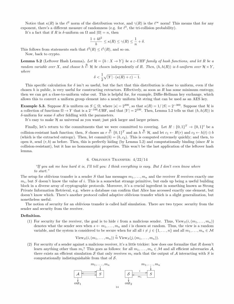
(2) For security of a sender against a malicious receiver, it’s a little trickier: how does one formalize that R doesn’tlearn anything other than mi? This goes as follows: for all m1, . . . ,mn ∈M and all efficient adversaries A,there exists an efficient simulation S that only receives mi such that the output of A interacting with S iscomputationally indistinguishable from that of S.

m1, . . . ,mn

A

////

Soo

out1

m1, . . . ,mn

S

i //

Smi

oo

out214

Then, we require that out1c≈ out2.

This is called half simulation because the simulation security definition is used for one side of the exchange, butnot the other.

It’s an easy exercise that oblivious transfer implies key exchange secure against eavesdropping (and it also impliesa lot more for multi-party computation). But this means that it can’t be built from AES-like techniques, and insteadwe need algebra. A simple construction uses something called blind signatures: given some key-generating algorithm(sx, px) ← KeyGen(), the sender S has a secret key sk and a public key pk, such that (after perhaps some morecommunications), the receiver R signs a message m ∈ M, obtaining σ. Then, it’s required for the signature to beunique, i.e. this σ is the only such one such that V (pk,m, σ) = 1. (Such schemes have been constructed, dependingon factoring being hard, etc.)

This doesn’t really work with existential unforgeability as we have seen it, so it has to be relaxed: given a public keypk, an adversary can make q signature requests for messages m, and this adversary wins if it can output q + 1 validmessage-signature pairs. A system is called unforgeable if it is secure against such games (in the usual probabilisticsense); this is the notion of sender security.

For recipient security, the adversary sends the challenger the public key pk and two messages m0 and m1, whichchooses some b ∈ 0, 1 and signs mb. Then, the adversary tries to guess the value of b; the scheme is secure if theadversary’s advantage ie negligible.

Here are some examples of this.

Example 6.1.

(1) From RSA, let KeyGen choose primes p and q and N ← pq, and lets 3 be the public exponent (so thatgcd(3, ϕ(N)) = 1). Then, the public key is (N, e), and the secret key is (N, 3−1 mod ϕ(N) = d). We alsowant to have a hash function H :M→ ZN lying around. Thus, to turn this into a blind signature scheme,

the receiver chooses an rR← ZN , and then send to S y ← H(m) · r3 ∈ ZN , so it can compute the cube root

z ← y1/3 in ZN . Then, the signature is σ = z/r ∈ ZN .This ends up being consistent, because σ3 = (y1/3/r)3 = y/r3 = H(m). But is it secure? For sender

security, this boils down to the RSA assumption, assuming H is a random oracle. For recipient security, itseems reasonable, but the adversary can choose the public key; specifically, the adversary may choose N suchthat 3 | ϕ(N). This is hard to test (especially compared to whether 2 | ϕ(N), which boils down to p and qbeing odd) — or rather, it seems like it ought to be easy, but lots of work has been spent on it. Nonetheless,there are plenty of protcols created and used based on the assumption that determining whether e | ϕ(N) ishard (for e ≥ 3).

In any case, if 3 | ϕ(N), then the cubes are a strict subgroup of ZN , and in particular, r3 isn’t uniformin ZN . Thus, we might have that H(m) doesn’t have a cube root, in which case S learns this when it failsto compute z. But this means S learns something about the message signed, which is no good (specifically,whether it’s a cubic residue or not).

For reference, this is a forty-year-old security protocol, but was only recently shown to be insecure; this isone of the important points of choosing the right definition!

The way around this is to make the public key contain a zero-knowledge proof that 3 - ϕ(N) (which makesthis protocol, and the oblivious transfer protocol based on that, secure).

(2) There’s another protocol named BLS, which involves dealing with the notion of bilinear maps.

Definition. Let G be a group of prime order and g be a generator for G, and let GT be some other group(called the target group). Then, a bilinear map on G is a map e : G×G→ GT such that:• e is efficiently computable,• e(g, g) 6= 1, and• for all a, b, e(ga, gb) = e(g, g)ab.12

This lends itself nicely to a signature scheme: let p be prime and g generate G, a group of order p. Then,

let αR← Zp, and the secret key is α and the public key is gα. Then, letting H :M→ G be a hash as before,

the signature is S(sk,m) = H(m)α, and verification involves checking that e(gα, H(m)) = e(g, σ) (sincee(ga, h) = e(g, ha)).

Theorem 6.2. The BLS signature is existentially unforgeable if H is a random oracle and the computationalDiffie-Hellman assumption holds in G.

12Interestingly enough, these were discovered by a mathematician who was in jail for being a deserter from the French army in WorldWar II (though he called himself a conscientious objector). This period of his life was so productive he later wrote a letter suggesting that

all mathematicians be required to spend two years in jail!

15

This is all fine, but the point is to turn this into a blindable scheme as follows: the receiver has access tothe public key and some m ∈M. Then, it sends y ← H(m) · gr ∈ G, and the sender responds with z ← yα.The signature thus is σ ← z/(gα)r. Now, no zero-knowledge proof is needed to validate the public key; that gis a generator is as easy as checking g 6= 1 (since p is prime). It’s also a unique signature.

Blind signature schemes are used for anonymous voting systems, anonymous cash, and so on; today, we’ll be usingthem to construct oblivious transfer.

We start with unique blind signaturesMsig parameterized by [n] = 1, . . . , n and a hash H : [n]×Msig → 0, 1`that is a random oracle. Then, after a public key and secret key are chosen, the sender generates n ciphertexts viaσi ← S(sk, i) (where i is in a sense the message sent by the receiver), and then the final ciphertext is ci ← H(i, σi)⊕mi:in a sense, we use the hash as a one-time pad to enode mi. Then, the sender sends pk, c1, . . . , cn to the receiver,which outputs ci ⊕H(i, σi).

This will end up being secure, though this has to be proven. But there’s a very nifty property: this protocol ofasking for messages repeatedly can be repeated over and over. For example, a Netflix user can request a movie, havea one-time penalty of downloading the entire encrypted database, and then each purchase is a quick interaction withthe server.

Recipient security follows from that for the blind signature, but sender security is a little harder. Intuitively,given an efficient adversary A, a trusted T generates a public key and a secret key (pk, sk) via KeyGen, and creates

c1, . . . , cnR← 0, 1` (encryption of garbage), and sends the public key and these c1, . . . , cn to the adversary. Then, the

adversary sends back some blind signature and a random oracle query for H(j, σ). If the verification of the signatureindicates it’s correct, then T indicates mj , and we send cj ⊕mj to the adversary. But if verificaton fails, then wereturn random junk cj . Then, the adversary may output.

The point is, we are able to program the random oracle, and the system is secure if we can produce the same thingthe adversary does in some sense. But we’re toast if the adversary can somehow issue two queries with the same validsignature, since we can’t query the trusted source T , so if this is built on a forgeable scheme, then this can’t work,and in fact this simulation can be used to forge signatures if such an efficient adversary exists.

7. Oblivious Transfer II: 4/24/14

“I don’t understand; a filesystem is just a sequence of bits. Just encrypt it — what more is there tosay?”

Recall that last time, we introduced oblivious transfer, where a sender S has x1, . . . , xn ∈ X and the receiver Rrequests some xi for i ∈ [n]; the system has sender security if R can learn xi and nothing else, and has receiversecurity if S learns nothing abut i. The example we saw was based on blind signatures, and is a very natural protocol:it can be used to build a large number of other cryptogaphic protocols.

For example, here’s a protocol due to Bellare and Micali, which is based on the computational Diffie-Hellmanassumption. Let G be a group of prime order p with a generator g ∈ G. This will be a 1-out-of-2 oblivious transfer,i.e. the sender has two values m0,m1 ∈ 0, 1`, and the receiver has a bit b ∈ 0, 1 (corresponding to whether it asksfor m0 or m1). We also need a hash function H : G→ 0, 1`. Then, here’s how the protocol works:

(1) First, the sender gets a cR← G and sends it to the receiver.

(2) Then, the receiver gets a kR← Zp and generates two ElGamal secret keys yb ← gk and y1−b

R← c/gk¡ so thatR knows the discrete log of one of y0 or y1, but not both (intuitively, this would allow R to compute thediscrete log of c). Then, R sends y0 and y1 to S.

(3) The sender checks that y0 · y1 = c, and aborts if not (since this would destroy sender security).(4) Now, the sender computes a standard ElGamal encryption: it chooses r0, r1 ← Z∗p and sets c0 ← (gr0 , H(yr00 )⊕

m0) and c1 ← (gr1 , H(yr11 )⊕m1) and sends them to the receiver.(5) Finally, the receiver decrypts cb = (v0, v1) (standard ElGamal decryption) and outputs H(vk0 )⊕ v1 = mb.

For recipient security, we have information-theoretic security: the sender sees the same distribution on y0 and y1, nomatter the value of b, so it can’t tell the value of b from them. Sender security is a little more involved, but is similarto a proof we did last time. depending on the computational Diffie-Hellman assumption.

There is a similarly elegant but slightly more complicated protocol in which the sender has information-theoreticsecurity and the receiver has security based on the Diffie-Hellman assumption.13 However, neither this nor theprevious one are efficient enough for the real world.

For this one turns to oblivious transfer with preprocessing. Before any messages are received, the sender buildsmany pairs y0, y1), and the recipient has some bit k and yk (from the same source). Then, the online step is for R to

13Naor, M and Pinkas, B. Efficient oblivious transfer protocols. SODA ’01.

16

send c← b⊕ k to S, which responds with z0 = yc ⊕ x0 and z1 = y1−c ⊕ x1, and the receiver outputs zb ⊕ yk. This isvery fast: three ⊕ computations take nearly no time.14 As for why zb ⊕ yk = yb, this can be seen by a brute-forcechecking of cases: if b = 0, then

zb ⊕ yk = (yc ⊕ x0)⊕ yk = yk ⊕ x0 ⊕ yk = x0.

The case b = 1 is similar. Note also that c can be generated from a hash function starting with some publicly knownvalue.

Recipient privacy is pretty self-evident: S only sees a one-time pad encryption of k, and sender privacy followsbecause R only knows y0 or y1, and the other has one-time pad security.

This leads to a notion called oblivious polynomial evaluation, in which the sender S has some f ∈ Fp[x] and thereceiver has some y ∈ Fp; then, at the end of the protocol, R has f(y); the goal is for the amount of communicationto be o(deg f). This is useful because polynomial oblivious transfer implies 1-out-of-n oblivious transfer: if R hassome i ∈ [n] and S has a1, . . . , an, so it picks a random f of degree n+ 1 such that f(i) = ai for all i ∈ [n] (so thatthe value of f at i doesn’t leak any information about the other values — but this only admits one query), and thuscan overlay this on top of an existing oblivious transfer protocol.

It also implies a comparison protocol, where S has a b ∈ Fp and R has an a ∈ Fp; then, they want to check if they’re

equal, but not leak any more information if they’re not. In this case, S picks some rR← F∗p and lets f(x) = r(x− a);

then, if a = b, then f(b) = 0, and otherwise, its value is random in F∗p. (The specifics of the transfer boil down tothe polynomial evaluation protocol from before.) Often, for p large, one can use Fp instead of F∗p; their statisticaldependence lessens and lessens. This protocol is useful in, for example, password authentication.

This can also be used to determine set membership! Here, the sender has a set A = a1, . . . , an ⊆ Fp, and therecipient has a b ∈ Fp and wants to know if b ∈ A. This might be useful if you want to check if you’re on the no-flylist for the TSA without revealing your identity. This boils down to polynomial evaluation of

f(x) = r ·n∏i=1

(x− ai)

at b, where r is random inZ∗p.Finally, one can use this to make oblivious PRFs F : K × X → Y . The idea is that the sender has a k ∈ K

and the receiver has an x ∈ X, and wants to know F (k, x) without leaking x to S or k to R. One technique is theNaor-Reingold PRF, which is efficient (and doesn’t depend on the polynomial evaluation protocol described above).It leads to a nice protocol for set membership: first, S chooses a k ← K, and then sends F (k, a1), . . . , F (k, an); then,the receiver can determine F (k, b) without k or the sender knowing b, and then determine if the value is in one of theF (k, ai). (Then, this implies set intersection, etc.)

Private Information Retrieval (PIR). This is related to oblivious transfer; here, the sender has some databasex1, . . . , xn ⊆ 0, 1`, and the receiver has an i ∈ [n], and learns xi and possibly other things, but the sender learnsnothing from R (we only care about recipient privacy). Trivially, S could send everything, but the goal is to minimizecommunication. A classic example is a patent database: it’s fine to see other patents than the one extracted, but onemight not want to broadcast which patents they read.

For a warm-up, there’s a more practical but much less cool protocol called two-server PIR, where S1 holdsx1, . . . , xn ∈ Fp and S2 also has a copy of x1, . . . , xn ∈ Fp, and S1 and S2 don’t talk to each other. Then, the recipienttalks to both S1 and S2 an obtains xi and possibly other stuff, and as long as S1 and S2 don’t communicate, we haveprivacy.15

There’s a somewhat trivial, but not as trivial, protocol that takes O(√n) traffic.16 Introduce the matrix

A =

x1,1 · · · x1,√n

.... . .

...x√n,1 · · · x√n,

√n

∈ F√n×√n

p .

Here, the sequence of n elements is represented as a matrix, so the indexing is rearranged slightly (and R is interestedin (i, j)). The naıve idea of asking S1 for the column in question and S2 for the row in question leaks informationabout which row or column the object of interest is in, which isn’t good. But instead, one could obtain that from Aei.

So to mask this, R chooses two vectors v1, v2 ← F√n

p such that v1 + v2 = ei ∈ F√n

p . Then, from the perspective of S1

or S2, these vi are uniformly random. Then, they send back Av1 = u1 and Av2 = u2; then, the recipient adds them

14A similar protocol is done for RSA signature schemes (and can be generalized to others), where the time-intensive computations are

done offline, making signing things much faster or on small devices such as smart cards or watches or whatnot.15You can probably guess how to generalize this to n-server PIR.16In general, when you see something that takes O(

√n) time, space, or traffic, always think about matrices!

17

to get u1 + u2 = A(v1 + v2) = Aei, and so we get the point the recipient is interested in. Since v1 and v2 are bothindependent of i and j, then this is secure. It’s fast from a network standpoint, but matrix multiplication requires theserver to look at every database entry, which seems inefficient. But this is necessary, because if the server doesn’tneed to look at an element, then the user doesn’t need it somehow (which is mitigated by the presence of the otherserver, but only by a factor of 2). Then, 2

√n elements are sent back and forth, which is the correct amount.

It turns out there’s a way to make 2-server PIR work with O( 3√n) communication, and this is the best one can do.

Can we do better than that with 3 servers? It was an open problem for a long time, but in 2009 a better bound of

O(26√

logn log logn) was discovered. This is nε for all ε, so it was quite a surprise. And this might not even be atight bound. Importantly, all of these results are information-theoretic, which can be done because the servers don’tcollude.

However, returning to the single-server case, one can show that a sublinear PIR algorithm implies collision-resistance,and thus we’ll need some complexity assumptions. However, for all ε > 0, there’s an o(nε) protocol using additivelyhomomorphic encryption, and there’s an o(log n) protocol based on an assumption called the φ-hiding assumption.(This assumption is still open, but the professor hopes it’s false.)

Let `1, . . . , `n be the first n primes, so that `n ≈ n lnn. Suppose the sender S has a database x1, . . . , xn ∈ 0, 1(a database of bits, like a theoretician’s view), and the receiver wants to know about some i ∈ [n]. Then:

(1) R chooses p, qR← Primes(λ) (i.e. λ-bit functions), for some λ, and such that p ≡ 1 (mod `i). Then, it sets

N ← pq, and chooses a wR← ZN such that w doesn’t have an `thi root in ZN (i.e. that w(p−1)/`i 6≡ 1 (mod p)).

Then, send N and w to the server.(2) S starts taking powers of w, getting

a← w∏nj=1 `

xjj ∈ ZN ,

in some sense taking exactly the primes such that xn = 1. This is a pretty crazy exponentiation, but S sendsa to R, so there’s not much traffic.

(3) Finally, the receiver calculates a(p−1)/`i mod p, which is 1 iff xi = 1, and otherwise, xi = 0.

Why does this work?

a(p−1)/`i =(w

∏nj=1 `

xjj

)p−1

≡ 1 iff xi = 1,

The communication is 3 elements of ZN , but N = o(n lnn), so there are o(log n) communication bits (which is verylow). As for security, the sender sees n and w. Do they leak information about i? Unfortunately, this involves thestandard trick in crypto: that they don’t.

More formally (and elegantly), the φ-hiding assumption claims that the following two distributions are indistin-

guishable for all ` < λo(1): choose p, q R← Primes(λ) such that p ≡ 1 mod `, and sR← ZN such that s isn’t an `th

residue; then, output (pq, s), compared with the distribution where ` might or might not divide φ(n) (unlike theprevious distribution, where ` | φ(n)), implying the name. This seems suspicious, but is still open.

8. Zero-Knowledge Proofs: 4/29/14

“Now, whenever you think about graph isomorphism, you’re going to think about milk.”

Before discussing interactive proof systems, let’s mention the complexity heirarchy: there are deterministic polynomial-time functions P, and on top of that NP and coNP both containing P, followed by a whole polynomial heirarchy,and PSPACE. There’s more on both ends, but this is what we want for now.

It’s useful to have that if L ∈ NP, then there exists a deterministic polynomial-time algorithm V : Σ∗×Σ∗ → 0, 1such that x ∈ L iff there exists a p ∈ Σ∗ such that V (x, p) = 1. V is said to be a verifier, and p is a short proof thatx ∈ L.

We can extend this model in a number of ways.

(1) What if V is randomized? Specifically, we require that if x ∈ L, Pr[V (x, p) = 1] ≥ 2/3 for some p ∈ Σ∗. Thiscomplexity class is called MA, for Merlin-Arthur (thanks to a scenario where Arthur calls upon his oracleMerlin to answer questions).

(2) What if V can only read the first 3 bits of P? This class is known as PCP, and one of the deepest theoremsin computer science is that PCP = NP, which could take a whole quarter to prove.

(3) What if the prover and verifier are allowed to interact? Here, P and V both share x, but are allowed to sharemessages back and forth, and eventually V emits one of 0 or 1. The class of strings which P can convince Vare in the language is known as IP (interactive proofs).

The last class, IP, is the most useful for crypto, and will be focused upon here.18

Definition. An interactive proof system for an L ⊆ 0, 1∗ is a two-party protocol17 between a probabilisticpolynomial-time verifier V and an infinitely powerful prover P sharing an x ∈ L satisfying the following properties.

(1) Completeness: for all x ∈ L, V always accepts x after interacting with P .(2) Soundness: for all x 6∈ L and all “bad” provers P ∗, V rejects with probability greater than18 1/2 after

interacting with P ∗.

Then, one can formally define IP to be all languages L ⊆ 0, 1∗ that are recognizable by an interactive proof system(i.e., there exist V and P such that the language recognized by them is L). Additionally, define IP(m) to be the set oflanguages in 0, 1∗ which are recognizable by an interactive proof of at most m rounds (P and V can send at mostm messages together).

First, note that NP ⊆ MA, since any deterministic verifier can be superseded by a randomized verifier. But, moreinterestingly, MA ⊆ IP(1), given by the algorithm where P sends a proof, and V checks it. And then it seems thatIP(1) ⊆ IP(2) ⊆ IP(3) ⊆ · · · , but it turns out that MA = IP(m)!

However, if one forces V to be deterministic, then the class of languags recognized is exactly NP, so the fact thatV can be randomized is what makes this very interesting: this is because it reduces to P sending one message to V ,but then this is just polynomial-time verification.

Example 8.1. Let’s look at the problem of graph isomorphism: if G1 = (V1, E1) and G2 = (V2, E2) are graphs,then they’re considered isomorphic if there exists a π : V1 → V2 such that (v1, v2) ∈ E1 iff (π(v1), π(v2)) ∈ E2 for allv1, v2 ∈ V1.

The problem of determining whether two graphs are isomorphic is in NP, and therefore there’s an interactiveproof (where the prover just sends the isomorphism to the verifier; soundness and completeness follow). But graphnon-isomorphism (i.e. proving two graphs aren’t isomorphic) is also in IP, even though it’s believed to not be inNP.19

If P and V are looking at two graphs (G0, G1), then V picks a πR← Sn (i.e. the symmetric group on n elements,

the set of permutations of 1, . . . , n), and a bR← 0, 1, and then sends to P the graph G∗ = Gπb . Then, the prover

sends back a b′ ∈ 0, 1 and the verifier accepts if b = b′. This could be called the “milk game,” inspired by a similartesting experiment where the prover hid one glass of milk from the verifier and asked her to guess what it was.

In the case of an honest prover (completeness), it’s infinitely powerful, so it can determine which of G0 or G1 wasused, so it sends back that particular value of b, and it’s sound, because a bad prover won’t be able to come up withan isomorphism if there isn’t one, so Pr[b = b′] = 1/2.

Here’s a few facts to keep in mind.

• The prover P only needs to be PSPACE, and sometimes, we’ll want more efficient provers.• There’s another formalism called Arthur-Merlin games,20 in which the verifier is only allowed to send random

values to the prover, which then responds; in this case, the verifier is called Arthur, and and the prover iscalled Merlin. This class of problems is called AM∗. Then, there’s a theorem that AM∗ = IP. This is kind ofinteresting; if your questions are random enough, you don’t actually need to think about what to ask.

So, where does IP actually live in the complexity heirarchy? There’s a beautiful result:

Theorem 8.2. IP = PSPACE.

Proof sketch. We’ll start by showing that coNP ⊆ IP, which is already surprising. It’s enough to do this for anNP-complete laguage, e.g. that of 3-colorable graphs. Let G = (V,E) and n = |V |. Then, the goal is to prove that Gis not 3-colorable.

Define a polynomial from G as

PG(x1, . . . , xn) =∏

(u,v)∈E

(xu − xv).

Here, xi ∈ 0, 1, 2 should denote the color of vertex i, so if (x1, . . . , xn) is an invalid coloring, then PG(x1, . . . , xn) = 0,and if (x1, . . . , xn) is valid, PG(x1, . . . , xn) is nonzero. We want to make it exactly equal to 1, so let f(x) =

17This can be formally defined as a set of two Turing machines, each of which can write to tapes read by the other, and so on, but

that’s not the point.18It’s possible to change the bound without any difference, since repeating a randomized algorithm several times decreases the

porbability of a false positive.19Curiously enough, it’s known to be not NP-complete, and generating hard instances for it is difficult; heuristics for it work for many

kinds of graphs.20This was invented by Babai of the University of Chicago in the 1990s, not by King Arthur (and Merlin) of Camelot in the Middle

Ages.

19

(5/4)x2 − (1/4)x4, which was chosen so that f(0) = 0 and f(1) = f(2) = f(−1) = f(−2) = 1. Then, redefine

PG(x1, . . . , xn) =∏

(u,v)∈E

f(xu − xv).

Now, PG(x1, . . . , xn) = 1 iff (x1, . . . , xn) is valid, and is 0 otherwise. Now, define

S =∑

x1∈0,1,2

∑x2∈0,1,2

· · ·∑

xn∈0,1,2

PG(x1, . . . , xn),

which is the number of valid 3-colorings of G (so we want to know whether S = 0).21.Now, we introduce the prover and verifier, which have access to PG and S. Choose a prime p > 4 |V |λ (where λ is

some large security parameter depending on |V |), and define

P1(x) =∑

x2∈0,1,2

∑x3∈0,1,2

· · ·∑

xn∈0,1,2

PG(x, x2, . . . , xn).

Then, deg(P1) < 4n, 4 from f . Then, P sends the coefficients of some polynomial P1 to V (an honest prover would

send over P1), which checks that P1(0) + P1(1) + P2(2) = S, and aborts if this isn’t true, since this is true for P1.

Then, the verifier chooses an rR← Fp and emits 1 if P1(r) = P1(r) and 0 otherwise (since random polynomials are

unlikely to have the same values on large Fp).But how does the verifier compute S1 = P1(r)? Well now, the verifier has P1(r) and the prover and verifier are

trying to compute on the value

S1 =∑

x2∈0,1,2

∑x3∈0,1,2

· · ·∑

xn∈0,1,2

PG(x1, . . . , xn),

so it’s possible for the protocol to just recurse until the verifier can just compute the last two or three summations bybrute-force. Then, it unravels everything, and then verifier is convinced that everything is correct.

Thus, this is a 2n-round Arthur-Merlin protocol, and it’s crucial that the randomness is chosen after the proversends over its answer each time.

The general proof for PSPACE has very similar principles.

This also shows that AM∗ = IP, too.The idea is that for sufficiently large polynomials, if they agree at a random point, they almost certainly agree.

This is an easy way to test whether two polynomials are equal, and comes up again and again in computer science.For example, one might test equality of sets by generating two polynomials whose roots are exatly the elements ineach set, and then checking if the polynomials are equal. Note that this algebraic proof is the only one the professorknows about.

Interactive proof systems are said to be zero-knowledge if the proof doesn’t leak any information to V that itdoesn’t already have.

Definition. A perfect zero-knowledge proof for a language L ⊆ 0, 1∗ is a proof system (P, V ) for L (i.e. itis complete and sound) such that for every probabilistic polynomial-time verifier V ∗, there exists a probabilisticpolynomial-time simulator S∗ such that for all x ∈ L, the following distributions are the same:

transcript(P (x)←→ V ∗(x)) = S∗(x).

This means that anything that V ∗ could have learned from P can be determined from x already, so V ∗ doesn’tlearn anything from P , beyond the fact that x ∈ L. Note that if x 6∈ L, then there’s no restriction; intuitively, ifyou’re trying to prove the false fact that x ∈ L, then something is already going wrong, and information leaking isless of a concern.

The original paper by Goldwasser and Micali is a classic in crypto; yet it was rejected three times (albeit from thesame journal) before being accepted. We’ll write out an example now, but prove that it’s zero-knowledge next time.

Remark. If perfectly hiding commitments exist, then every L ∈ PSPACE (i.e. anything that can be proven interactively)has a zero-knowledge proof.

This was quite a surprise when it was discovered, though the proof boils down to showing that NP has zero-knowledge proofs (e.g. prove that 3-coloring has zero-knowledge proofs, which is easy), and then boost to PSPACE,which also isn’t hard.

21This comes from a class of problems known as #P (called sharp-P), which asks for counting problems, where there’s an integer

answer, rather than just 0, 120

Example 8.3. The example of quadratic reciprocity is very useful in crypto. Fix N = pq and x ∈ Z∗N ; the goal is toprove that x has a square root in Z∗N (which is only true for one-quarter of the elements). Detecting this from theground up is hard (albeit not as hard as factoring), and there’s an easy interactive proof, given by just sending asquare root over. But this isn’t zero-knowledge.

In a zero-knowledge protocol, the prover is defending itself from a malicious verifier, so it’ll use a blinding; it

chooses some rR← ZN and send over a = r2 (mod N). Then, the verifier chooses a b

R← 0, 1, and sends it to P .Then, the prover sends back c← r ·αb ∈ ZN , where α ≡ x2 (mod N), and the verifier checks that c2 = axb (mod N),and accepts if so.

What’s going on is that the prover either sends r, or rα; in the first case, where b = 0, the verifier learns thesquare root of a random square, which isn’t of much use to it. But the blinding in the case b = 1 will make thiszero-knowledge. The fact that b is randomly chosen is there to keep P honest: otherwise, if it were always 1, then Pcould cook up a seed such that every number is “proven” to be a quadratic residue.

10. Zero-Knowledge Proofs III: 5/6/14

Today’s lecture was given by Mark Zhandry, the TA, since Dan Boneh is out of town.Recall that the general setup for a zero-knowledge proof is that there is a statement x to prove and a prover P and

verivier V who exchange messages; eventually, the verifier either accepts or rejects. For this to be a zero-knowledgeproof we require the following.

• The protocol should be complete, i.e. if x is true, then V accepts. More formally,

Pr [P (x)! V (x) : V accepts] = 1,

where P (x)! V (x) symbolizes the interaction between the prover and the verifier.• The protocol should be sound : for all cheating provers P ′, V rejects false statements x with reasonable

probability (usually, but not always, the probability that V accepts in this case is negligible).• The protocol should be, of course, zero-knowledge: in the case where x is true, the verifier learns nothing but

the truth of x. More formally, for all cheating verifiers V ′, there exists a simulator S such that

S(x) ≈ ViewV ′ [P (x)! V ′(x)].

This notation refers to what V ′ learns.

As an example, consider the Chaum-Pedersen proofs that a tuple is actually a DDH tuple (i.e. (g, ga, gb.gc) =(g,X, Y, Z) such that c = ab). Here’s a protocol for proving it:

(1) The prover chooses a random sR← Zq, and sends to the verifier V = gs and W = Xs.

(2) Then, the verifier chooses a tR← Zq and sends it to P .

(3) Next, the prover sends back U = s+ bt.(4) The verifier accepts iff gU = V Y t and XU = WZt.

Why is this a zero-knowledge protocol?

• For completeness, if this is really a DDH tuple, then V Y t = gsgbt = gs+bt = gU , and WZt = gasgabt =ga(s+bt) = gaU = XU .

• For soundness, suppose the prover cheats: V = gs and W = Xs′ for some s′ not necessarily equal to s. Afterreceiving a t, the false prover has to come up with a U that makes the two equations hold, but there is nochoice of s, s, and U that make the equations hold. This is because V Y t = gs+bt = gU , so U = s+ bt andWZt = gas

′gct = gaU , so aU = as′ + ct. Rearranging these a bit, a(s− s′) = (ab− c)t. But the right-hand

side is something nonzero, multiplied by a random element in Zq, so it’s a random element in Zq, so theprobability of the false prover succeeding is negligible (probability 1/q).

• Finally, we should prove that this protocol is zero-knowledge for verifiers that generate t before seeing V

and W . Given some verificiation algorithm V ′, define a simulator S that chooses vR← Zq, and run V ′ to

get t. Then, set V = gv/Y t and W = Xv/Zt, and one can show that the transcript of S provides no extrainformation.22

Now, let’s look at an application of these Chaum-Pedersen proofs, to prove that two ElGamal ciphertexts encryptsome common message. Recall that this involves choosing a secret key sk = z ∈ Zq and pk = h = gx. Then, to

encrypt, Enc(h,m) chooses an rR← Za, and then the ciphertext is (gr, hr ·m), and decrypting Dec(x, c1, c2) sets

c2/cx1 = hr ·m/grx = m.

22The verifier is described as both cheating and honest: this means that it can choose t arbitrarily so long as it does so before seeing V

and W .

21

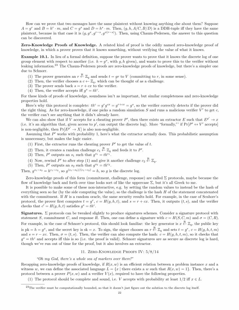
How can we prove that two messages have the same plaintext without knowing anything else about them? SupposeA = gr and B = hr ·m, and C = gs and D = hs ·m. Then, (g, h,A/C,B/D) is a DDH-tuple iff they have the sameplaintext, because in that case it is (g, gx, gr−s, gx(r−s)). Then, using Chaum-Pedersen, the answer to this questioncan be discovered.

Zero-Knowledge Proofs of Knowledge. A related kind of proof is the oddly named zero-knowledge proof ofknowledge, in which a prover proves that it knows something, without verifying the value of what it knows.

Example 10.1. In lieu of a formal definition, suppose the prover wants to prove that it knows the discrete log of onegroup element with respect to another (i.e. h = gx, with g, h given), and wants to prove this to the verifier withoutleaking information.23 The Chaum-Pedersen proofs are zero-knowledge proofs of knowledge, but there’s a simpler onedue to Schnorr.

(1) The prover generates an rR← Zq and sends t = gr to V (committing to r, in some sense).

(2) Then, the verifier chooses a c← Zq, which can be thought of as a challenge.(3) The prover sends back s = r + cx to the verifier.(4) Then, the verifier accepts iff gs = thc.

For these kinds of proofs of knowledge, soundness isn’t as important, but similar completeness and zero-knowledgeproperties hold.

Here’s why this protocol is complete: thc = grgcx = gr+cx = gs, so the verifier correctly detects if the prover didthe right thing. As for zero-knowledge, if one picks a random simulation S and runs a malicious verifier V ′ to get c,the verifier can’t see anything that it didn’t already have.

We can also show that if V accepts for a cheating prover P ′, then there exists an extractor E such that Ep′ → x

(i.e. it’s an algorithm that, given access to p′, can output the discrete log). More “formally,”’ if Pr[P ′ ↔ V ′ accepts]

is non-negligible, then Pr[Ep′ → X] is also non-negligible.

Assuming that P ′ works with probability 1, here’s what the extractor actually does. This probabilistic assumptionis unnecessary, but makes the logic easier.

(1) First, the extractor runs the cheating prover P ′ to get the value of t.

(2) Then, it creates a random challenge c1R← Zq and feeds it to P ′.

(3) Then, P ′ outputs an s1 such that gs1 = thc1 .

(4) Now, rewind P ′ to after step (1) and give it another challenge c2R← Zq.

(5) Then, P ′ outputs an s2 such that gs2 = thc2 .

Then, gs1−s2 = hc1−c2 , so g(s1−s2)/(c1−c2) = h, so g is the discrete log.

Zero-knowledge proofs of this form (commitment, challenge, response) are called Σ protocols, maybe because theflow of knowledge back and forth over time looks sort of like the uppercase Σ, but it’s all Greek to me.

It is possible to make some of these non-interactive, e.g. by setting the random values to instead be the hash ofeverything seen so far (by the side computing the value), so the challenge is the hash H of the statement concatenatedwith the commitment. If H is a random oracle, the same security results hold. For example, in the case of Scnhorr’sprotocol, the prover first computes t = gr, c = H(g, h, t), and s = r + cx. Then, it outputs (t, s), and the verifierchecks that c′ = H(g, h, t) satisfies gs = thc.

Signatures. Σ protocols can be tweaked slightly to produce signatures schemes. Consider a signature protocol withstatement S, commitment C, and response R. Then, one can define a signature with c = H(S,C,m) and σ = (C,R).

For example, in the case of Schnorr’s protocol, this should look familiar: the key generator is xR← Zq, the public key

is pk = h = gx, and the secret key is sk = x. To sign, the signer chooses an rR← Zq and sets t = gr, c = H(g, h, t,m)

and s = r − xc. Then, σ = (t, s). Then, the verifier can also compute the hash: c = H(g, h, t,m), so it checks thatgs = thc and accepts iff this is so (i.e. the proof is valid). Schnorr signatures are as secure as discrete log is hard,though we’ve run out of time for the proof, but it also involves an extractor.

11. Zero-Knowledge Proofs IV: 5/8/14

“Oh my God, there’s a whole sea of markers over there!”

Recapping zero-knowledge proofs of knowledge, if R(x,w) is an efficient relation between a problem instance x and awitness w, we can define the associated language L = x | there exists a w such that R(x,w) = 1. Then, there’s aprotocol between a prover P (x,w) and a verifier V (x), required to have the following properties.

(1) The protocol should be complete and sound, i.e. V accepts with probability at least 1/2 iff x ∈ L.

23The verifier must be computationally bounded, so that it doesn’t just figure out the solution to the discrete log itself.

22

(2) It’s zero-knowledge: for all verification algorithms V ∗ there exists a simulator S such that for all x ∈ L, thetranscript between the prover and the verifier is computationally indistinguishable to S∗(x).

There’s also a much weaker property called honest-verifier zero-knowledge, where the transcripts are only consideredfor honest verifiers. Formally, there exists a simulator S such that for all honest verifiers V ,

trans(P (x)←→ V (x))c≈ S(x).

We also talked about the proof-of-knowledge property: that there exists an extractor E for all provers P ∗ (includingmalicious ones) and x such that [P ∗(x)←→ V (x)] accepts.

As an example, if G is a group such that |G| = p and g, h ∈ G are generators of G, then we had zero-knowledgeproofs of the Diffie-Hellman language L = (g, , gα, hα) : α ∈ Zp, along with the Schnorr protocol for zero-knowledge

proof of knowledge R((g, h), w) = 1 iff gw = h: the prover chooses an rR← Zp and sends u = gr to V ; then, the verifier

computes a cR← [0, . . . , 2128] and sends it back. The prover then sends z ← r + c · w , and the verifier checks that

gz = uhc. This is a special case of a more general concept called a Σ protocol, where (u, r)← P0(sk) (generated from

a secret key using some protocol) is computed by P , which sends u to V ; then, V computes cR← [1, . . . , β] and sends

it to P . Finally, the prover computes a z ← P1(sk, r, c), and sends it to V , which computes T (pk, u, c, z) to determinewhether to accept or reject.

The Fiat-Shamir protocol allows this to be made non-interactive (i.e. P sends only one thing to V , and V sendsnothing to P ). Assuming we have a hash function H, one can compute c ← H(g, h, u) and then send z and u asnormal, and that if one appends m, instead calculating c ← H(g, h, u,m), then the result is a signature scheme(sig(m) = [u, z]), called Schnorr signatures. However, Schnorr patented his algorithm, so a different but relatedalgorithm, called DSA, is the federal standard. This, unlike DSA, has security. . .

Interestingly, this is noticeably shorter than the DSA signature. We have [u, z], where u ∈ G and z ∈ Zp, so if wework mod p, then u has to be about 2000 bits and z has to be about 256 bits, which is quite long. But Schnorr alsoapplied an optimization that allows one to shrink this signature: since the verifier just computes c from u and doesn’tuse the rest of the information, it’s possible to instead send [c, z], which allows the verifier to recompute u = gz/hc

and then recompute c = H(g, h, u,m) and check if c = c. But since z ∈ Zp and c is of size 128, this is going to onlybe about 400 bits, while DSA signatures are longer. Good thing Schnorr’s patent has expired, right? But since it’snot the federal standard, if you use it in a product, you can’t sell it to the government (which is part of why nobodyuses it).

Theorem 11.1. Schnorr signatures are existentially unforgeable under CMA, assuming H is a random oracle andthe discrete log is hard in G.

Proof sketch. Given some forger, consider an honest simulator S, and run it on an honest verifier. Choose somegenerators pk = (g, h) and send them to the forger; then, it sends back a message m, and run S to get (u, c, z), wherec is uniform in [0, . . . , β], and send (u, z) to the forger. Then, we can “program” H (the standard random oracle trick;this is OK, because c is uniform) such that H(g, h, u,m) = c. Then, if the forger can solve this, then it can break thediscrete log problem, and an extractor can (more or less) obtain the discrete log w.

Witness-Indistinguishable Proofs. As usual, suppose there’s a relation R(x,w) and an interactive systemP (x,w)←→ V (x).

Definition. The system (P, V ) is a witness-indistinguishable proof of knowledge if:

• for all (not necessarily honest) verifiers V ∗ and for all w0, w1 such that R(x,w0) = R(x,w1) = 1, then

tran(P (x, r0)←→ V ∗(x))c≈ tran(P (x,w1)←→ V ∗(x)).

• (P, V ) is zero-knowledge.

This is a pretty weak notion of security: this protocol doesn’t uniquely identify the witness, but it does leakinformation about it. Zero-knowledge proofs leak no information about the witness.

Lemma 11.2. All zero-knowledge proofs are witness-indistinguishable.

Proof. By the zero-knowledge property,

tran(P (x,w0)←→ V ∗(x))c≈ S∗(x)

c≈ tran(P (x,w1)←→ V ∗(x)).

Zero-knowledge is a much stronger property than witness indistinguishability. However, we don’t believe (this isactually still open) that zero-knowledge is maintained under parallel composition, whereas witness indistinguishabilityis (i.e. running the protocol in parallel 20 times); this is a simple hybrid argument.

23

Example 11.3. While any zero-knowledge proof is a witness-indistinguishable proof, it’s more interesting to give anexample that isn’t zero-knowledge. Recall that at least four interactions need to happen in any zero-knowledge proof,so consider the following shorter proof, called an OR proof.

We want to satisfy the property that R((g, h0, h1), w) = 1 iff gw = h0 or gw = h1, so consider the following

Schnorr-line protocol: if gw = h0, then choose an r0R← Zp and u0 ← gr0 . Then, inside the simulator, set u1 ← gz/hc1,

c1R← Z∗p, and z1

R← Zp; then, it sends u0 and u1 to the verifier V (g, h0, h1), which sends a cR← Z∗p back to the prover,

which sets c0 = c/c1. Finally, the prover sends z0 ← r0 + wc0, and sends c0, z0, z1 to the verifier, which checks thatfor b = 0, 1, gz0 = ubh

cbb , where c1 ← c/c0.

If instead gw = h1, then switch the order; these are called OR proofs because one or the other of the discrete logsis proved, but not both.

This protocol has lots of properties.

• It’s a proof of knowledge, in which you should extract some witness, because the extractor checks that ifgz = uhc and gz

′= uhc

′, then g(z−z′)/(c−c′) = h, so as long as c 6= c′, then this works. This is thus generalized

to allow the extractor to extract w0 if the prover has w0, or w1 if it has w1. Thus is independent of thewitness, so this works.• It’s also witness-indistinguishable. The transcript is in both cases (u0, u1, c, c0, z0, z1), but this isn’t computa-

tionally distinguishable: u0 and u1 are random elements in G, c is generated by a possibly malicious verifier,c0 is random in Z∗p in either case (though if we have to quotient then it’s slightly more complicated), and z0

and z1 are computed to pass the verification tests, so they’re the same in both cases. Thus, this transcripthas the same distribution in both cases.

• It’s also honest-verifier zero-knowledge, because the transcript can be simulated, where cR← Z∗p instead.

However, it’s not yet zero-knowledge (because it’s only got three rounds). By adding a commitment to c, itbecomes zero-knowledge, but then it’s not a proof of knowledge, because the extractor can’t go back andundo the commitment.

Here’s an “application” to identification protocols, which is sound but more complicated than other protocols forthe same result. However, the idea is still worth knowing for other applications.

An identification protocol is a way for a prover to prove its identity to a verifier (e.g. a car door which unlocks oncea specific person has proven its identity). The goal is to protect against eavesdropping security, where an attacker cansee many honest interactions between a prover and a verifier, but then cannot fool the verifier.

Let w be the secret key, held by the prover, and gw be the public key, held by the verifier. It’s possible to setup this protocol with challenge-response or even just one-time passwords, But there’s a protocol secure againsteavesdropping attacks based on an honest-verifier zero-knowledge proof of knowledge: if one has an attacker than canfool the verifier, then the honest interactions it watched can be simulated, and then the extractor can be used to getthe attacker to break the discrete log.

Active security is more interesting: the attacker can interact with the prover (e.g. a fake ATM in the mall), andthen the attacker can masquerade with the prover as the verifier. One-time passwords aren’t actively secure, becauseone could collect a one-time password and feed it to the verifier. However, challenge-response protocols are securehere (relying on an underlying secure signature scheme).24

Proposition 11.4. Witness indistinguishability implies identification protocols secure against active attackers.

Proof. Consider a proof system where the prover P has (g, h0, h1, w), and the verifier V has (g, h0, h1). Then, theyexecute the witness-indistinguishable OR protocol as before.

Suppose there exists an active attacker that can defeat this protocol; then, we will be able to use it to break thediscrete-log problem. We are given as input g and h = gα, and choose h0 and h1, so the public key is (g, h0, h1)

(which the attacker of course has access to). The trick will be to choose a random bit bR← 0, 1 and a random

rR← Zp, and let hb ← grbb and h1−b ← h, so we know the discrete log of exactly one, but the attacker doesn’t know

which. Then, the attacker makes a number of probes to try and determine the secret key.Since we know one of the discrete logs, we don’t need a simulator, and thus don’t need zero-knowledge.Now, the attacker tries to fool the verifier, but since it’s a proof of knowledge, we can extract a witness. . . and

there’s a 50% probability that it’s a witness for hb, which isn’t particularly helpful (so abort). Otherwise, we get thediscrete log of h, which is α, so the attacker can calculate discrete logs with probability 1/2.

24There’s another variant of challenge-response protocols using encryption, where the verifier sends a random encryption of a messagem, and the prover decrypts this message. It turns out the security property needed is CCA1 (or if that’s confusing, chosen ciphertext

security will do).

24

Notice that witness-indistinguishability is crucial so that the attacker can’t tell which witness is which, so it can’tforce failure. Thus, there’s a three-round active-ID protocol (i.e. secure against active attacks), and the security isbased on the discrete log, and no random oracles.

In the real world, of course, we can build signatures with a two-round protocol. However, without random oracles,we don’t now how to build them on the discrete log, and instead need stronger assumptions. Does the differencematter in practice? Maybe not.

12. Elliptic Curves: 5/13/14

“. . . and there’s no political subtext to labeling Democrats 0 and Republicans 1.”

For an application of proving relations with zero-knowledge, consider ElGamal encryption: suppose we have a publickey pk = (g, h) and |G| = p. Then, let c0 = (gα0 , hα0 · gm0), c1 = (gα1 , hα1 · gm1), and c2 = (gα2 , hα2 · gm2); then, thegoal is to show that m2 = m1 ·m0.

Proving addition (that is, m2 = m1 +m0) is easy, since we already have proof for Diffie-Hellman, so check this on(g, h,

c0[1] · c1[1]

c2[1],c0[0] · c1[0]

c2[0]

),

which forms a DDH tuple iff m2 = m1 +m0, so that the third term is hα0+α1−α2 and the fourth is gα0+α1−α2 , whichuses a Chaum-Pederson proof.

The proof for multiplication is much more involved, but has a nice application to voting protocols. Here, each userchooses a vi ∈ 0, 1, and sends E(pk, v1) = (gαi , hαi · gvi). Then, the center can compute

c∗ =

(n∏i=1

ci[0],

n∏i=1

ci[1]

),

which after decrypting is g∑vi . But since there aren’t that many votes, then the discrete log can be taken, yielding∑

vi, which provides the result.It’s a little uncomfortable that the center can decrypt individual users’ votes, but this can be alleviated by

distributing the key amongst several shared trustees. More problematic is that as is, this protocol has no protectionagainst the user ecrypting 30, or −12, or anything like that to make their vote count more than others’. Thus, alongwith its vote, a user should submit a zero-knowledge proof that its vote is eihter zero or one.

The most efficient way to do this is an OR proof: if c = (gα, hα · gm), one can prove that one of (g, h, c[0], c[1]) or(g, h, c[0], c[1]/g) is a DDH-tuple, so this uses the standard zero-knowledge proof. An alternate proof is to prove thatc is an encryption of m2, and then feed three copies into the multiplication checker. This tests that m2 = m, which isonly true for m = 0 and m = 1.

The History of Elliptic Curves. Moving on to elliptic curves: one could (and many do) spend one’s whole lifestudying elliptic curves. We’ll start with a history of why they’re interesting in general, and then why they’reinteresting for crypto specifically.

Elliptic curves combine all three branches of mathematics: algebra, analysis, and geometry, in a way that needs allof them. The history for algebra starts a pretty long time ago, in the days of Diophantus (in Alexandria, 200 AD).He wrote seven volumes called Arithmetica: they were stored in the Library of Alexandria for centuries, disappeared,and then four volumes popped up again in the Vatican library a millenium later. Probably by accident, someone hadgrabbed books from the Library of Alexandria, when it was burning or maybe earlier. One of these four was then lostat a later date. . .

Diophantus started by asking about rational solutions to the equation x2 +y2 = 1 (first asked by the Pythagoreans),which leads to integer solutions to x2 + y2 = z2. He may have been the first mathematician to think of fractions asnumbers. Then, he generalizes to other conics, e.g. ax2 + by2 + cxy + dx = 0, with a, b, c, d ∈ Z. For ax2 + by2 = 1, if

one has a solution y = ax+ b (i.e. one of its two solutions is rational), then the other root must also be rational. Thismeans that if one intersects the conic with any line through that rational point, then the other intersection are alsorational (though there are some conics without rational points, e.g. x2 + y2 = 3). Thus, there’s an easy map from therational numbers to rational points on conics, and it works in every field.

Then, he looked at problems such as x3 + y3 = z3, or really, what are the rational points on x3 + y3 = 1? Fermatsaid something about this later. Diophantus chose a really arbtrary-looking cubic y(6− y) = x3 − x. More generally,the goal is to understand rational points on curves of type y2 = x3 + ax + b, for a, b ∈ Q (i.e. the zero set off(x, y) = y2 − x3 − ax− b).

There are two special cases of note.25

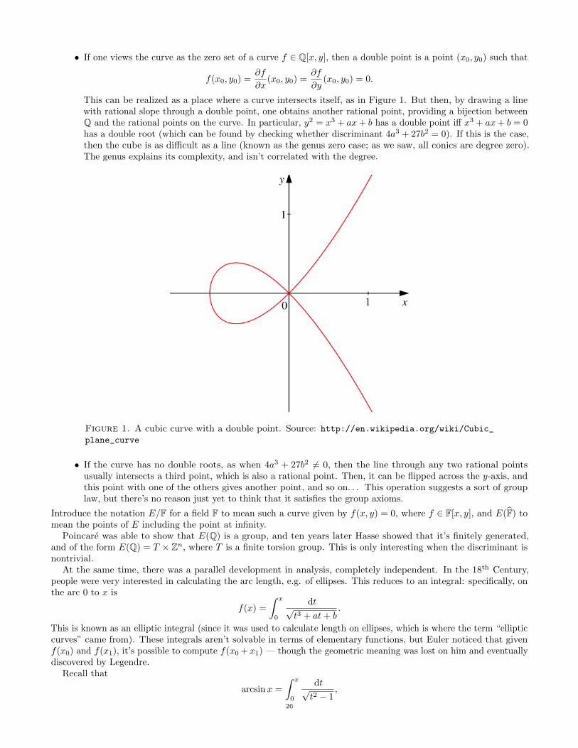
• If one views the curve as the zero set of a curve f ∈ Q[x, y], then a double point is a point (x0, y0) such that

f(x0, y0) =∂f

∂x(x0, y0) =

∂f

∂y(x0, y0) = 0.

This can be realized as a place where a curve intersects itself, as in Figure 1. But then, by drawing a linewith rational slope through a double point, one obtains another rational point, providing a bijection betweenQ and the rational points on the curve. In particular, y2 = x3 + ax+ b has a double point iff x3 + ax+ b = 0has a double root (which can be found by checking whether discriminant 4a3 + 27b2 = 0). If this is the case,then the cube is as difficult as a line (known as the genus zero case; as we saw, all conics are degree zero).The genus explains its complexity, and isn’t correlated with the degree.

Figure 1. A cubic curve with a double point. Source: http://en.wikipedia.org/wiki/Cubic_

plane_curve

• If the curve has no double roots, as when 4a3 + 27b2 6= 0, then the line through any two rational pointsusually intersects a third point, which is also a rational point. Then, it can be flipped across the y-axis, andthis point with one of the others gives another point, and so on. . . This operation suggests a sort of grouplaw, but there’s no reason just yet to think that it satisfies the group axioms.

Introduce the notation E/F for a field F to mean such a curve given by f(x, y) = 0, where f ∈ F[x, y], and E(F) tomean the points of E including the point at infinity.

Poincare was able to show that E(Q) is a group, and ten years later Hasse showed that it’s finitely generated,and of the form E(Q) = T × Zn, where T is a finite torsion group. This is only interesting when the discriminant isnontrivial.

At the same time, there was a parallel development in analysis, completely independent. In the 18th Century,people were very interested in calculating the arc length, e.g. of ellipses. This reduces to an integral: specifically, onthe arc 0 to x is

f(x) =

∫ x

0

dt√t3 + at+ b

.

This is known as an elliptic integral (since it was used to calculate length on ellipses, which is where the term “ellipticcurves” came from). These integrals aren’t solvable in terms of elementary functions, but Euler noticed that givenf(x0) and f(x1), it’s possible to compute f(x0 + x1) — though the geometric meaning was lost on him and eventuallydiscovered by Legendre.

Recall that

arcsinx =

∫ x

0

dt√t2 − 1

,

26

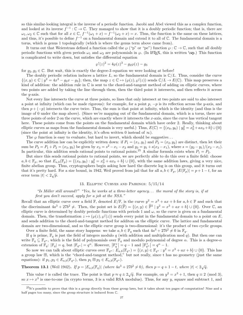
so this similar-looking integral is the inverse of a periodic function. Jacobi and Abel viewed this as a complex function,and looked at its inverse f−1 : C→ C. They managed to show that it is a doubly periodic function; that is, there areω1, ω2 ∈ C such that for all x ∈ C, f−1(ω1 + x) = f−1(ω2 + x) = x. Thus, the function is the same on these lattices,and thus, it’s possible to define f−1 on a fundamental domain and extend it to all of C. The fundamental domain is atorus, which is genus 1 topologically (which is where the genus term above came from).

It turns out that Weierstrass defined a function called the ℘ (“p” or “pe”) function ℘ : C→ C, such that all doublyperiodic functions with given periods ω1 and ω2 are polynomials in ℘. (In LATEX, this is written \wp.) This functionis complicated to write down, but satisfies the differential equation

℘′(z)2 = 4℘(z)3 − g2℘(z)− g3

for g2, g3 ∈ C. But wait, this is exactly the degree-3 equation we were looking at before!The doubly periodic relation induces a lattice L, so the fundamental domain is C/L. Thus, consider the curve

(x, y) ∈ C | y2 = 4x3 − g2x− g3; then, the map z ∈ C 7→ (℘(z), ℘′(z)) sends C/L→ E(C). This map preserves akind of addition: the addition rule in C is sent to the chord-and-tangent method of adding on elliptic curves, wheretwo points are added by taking the line through them, then the third point it intersects, and then reflects it acrossthe y-axis.

Not every line intersects the curve at three points, so lines that only intersect at two points are said to also intersecta point at infinity (which can be made rigorous): for example, for a point p, −p is its reflection across the y-axis, andthen p+ (−p) intersects the curve twice. Thus, the sum is that point at infinity, which is the identity (and thus is theimage of 0 under the map above). (Since we’re mapping out of the fundamental domain, which is a torus, there arethree points of order 2 on the curve, which are exactly where it intersects the x-axis, since the curve has vertical tangenthere. These points come from the points on the fundamental domain which have order 2. Really, thinking aboutelliptic curves as maps from the fundamental domain is very useful.) Thus, E(C) = (x0, y0) | y2

0 = x30 +ax0 + b∪0

(since the point at infinity is the identity, it’s often written 0 instead of ∞).The ℘ function is easy to evaluate, but hard to invert, which should be suggestive. . .The curve addition law can be explicitly written down: if P1 = (x1, y1) and P2 = (x2, y2) are distinct, then let their

sum be P3 = P1 +P2 = (x3, y3) be given by x3 = s2−x1−x2 and y3 = y1 + s(x3−x1), where s = (y2− y1)/(x2−x1).In particular, this addition sends rational points to rational points.25 A similar formula exists when P1 = P2.

But since this sends rational points to rational points, we are perfectly able to do this over a finite field: choosea, b ∈ Fp, so that Ea,b(Fp) = (x0, y0) : y2

0 = x30 + ax0 + b ∪ 0, with the same addition laws, giving a very nice,

finite abelian group. Thus, cryptographers begin asking how hard the discrete log is on this group, and it turns outthat it’s pretty hard. For a size bound, in 1942, Weil proved from jail that for all a, b ∈ Fp, |E(Fp)| = p+ 1− t, for anerror term |t| < 2

√p.

13. Elliptic Curves and Pairings: 5/15/14

“Is Miller still around?” “Yes, he works at a three-letter agency. . . the moral of the story is, if atfirst you don’t succeed, apply for a job at the NSA.”

Recall that an elliptic curve over a field F, denoted E/F, is the curve y2 = x3 + ax + b for a, b ∈ F and such that

the discriminant 4a3 + 27b2 6=. Then, the point set is E(F) = (x, y) ∈ F2 | y2 = x3 + ax + b ∪ 0. Over C, anelliptic curve is determined by doubly periodic functions with periods 1 and ω, so the curve is given on a fundamentaldomain. Then, the transformation z 7→ (℘(z), ℘′(z)) sends every point in the fundamental domain to a point on E,and sends addition to the chord-and-tangent method for additon on the elliptic curve. The lattice and fundamentaldomain are two-dimensional, and so the elliptic curve group is two-dimensional: it’s the product of two cyclic groups.

Over a finite field, the same story happens: we take a, b ∈ Fq such that 4a3 + 27b2 6= 0 in Fq.If q is prime, Fq is just the field of integers modulo q (with addition and multiplication mod q). But then one can

write Fq ⊆ Fqα , which is the field of polynomials over Fq and modulo polynomial of degree α. This is a degree-αextension of Fq: |Fq| = q, but |Fqα | = qα. However,

∣∣F×q ∣∣ = q − 1 and∣∣F×qα ∣∣ = qα − 1.

So now we can talk about elliptic curves over Fqα : Ea,b(Fqα) = (x, y) ∈ Fqα : y2 = x3 + ax+ b ∪ 0. This hasa group law , which is the “chord-and-tangent method,” but not really, since t has no geometry (just the sameequations): if p1, p2 ∈ Ea,b(Fqα), then p1 p2 ∈ Ea,b(Fqα).

Theorem 13.1 (Weil 1942). If p = |Ea,b(Fq)| (where 4a3 + 27b2 6= 0), then p = q + 1− t, where |t| < 2√q.

This value t is called the trace. The point is that p ≈ q ± 2√q. For example, on y2 = x3 + 1, then q ≡ 2 (mod 3),

so x 7→ x3 is one-to-one (in crypto terms, 3 is a valid RSA modulus). Thus, for any y, square and subtract 1, and

25It’s possible to prove that this is a group directly from these group laws, but it takes about ten pages of computation! Nine and a

half pages too many, since the group structure is induced from C.

27

thus there’s one value of x: thus, there’s one x for each y, plus the point at infinity, so p = q + 1. Thus, the trace iszero (sometimes, this is called a trace-zero curve).

Claim. If p = |E(Fq)|, then the sequence |E(Fq)| ,∣∣E(Fq2)

∣∣ , ∣∣E(Fq3)∣∣ , . . . is completely determined by p (once we

have t and q), and is in fact given by a nice generating function. This is useful for generating elliptic curves with agiven number of points: start by brute-forcing the number of points on a curve over Fq, and then extend it to someFqα .

Claim. Suppose that p - q(q − 1) (so we’re ignoring a few degenerate cases) and p is prime (so that E(Fq) is cyclic),and let α > 0 be the smallest integer such that p | qα − 1. Then, when we go to the extension, Z+

p (additive group of

integers mod p) appears twice: Z+p ×Z+

p ⊆ E(Fqα). One can sort of see this as a p× p lattice of order-p points in thisextension. This is no coincidence: it’s the same two-dimensionality as that from the complex numbers.

Now, thinking as cryptographers, here’s a new large group. So, how hard is discrete log? For random a, b ∈ Fq,the best-known discrete-log algorithm runs in time approximately O(

√q) = o(e(1/2) log q). For 128-bit security, one

needs q > 2256, and for 256-bit security, one wants a 512-bit modulus. Compare this to working in F∗q , where the

best algorithm has approximate running time of O(e3√

logn), which grows a lot because of the cube root! For 128-bitsecurity, one needs q > 22048, and for 256-bit security, one needs upwards of 215000, which is icky. Thus, the world ismoving towards elliptic curve cryptography, and specifically a curve called P256 (over 99% of large websites usingelliptic curves). How its parameters were obtained is a matter of great speculation, but we believe it to be secure:someone obtained random numbers and fed them through a SHA-256 hash to get the parameters.26 The discrepancyin eliptic-curve discrete-log and F∗q discrete-log is a twenty-year open problem.

For example, here’s the elliptic Diffie-Hellman protcol. Alice and Bob each respectively choose an aR← 1, . . . , |P256|

and a bR← 1, . . . , |P256|. Then, Alice sends A ← a · P to Bob (this · means repeated doubling), and Bob sends

B ← b · P . Then, each of Alice and Bob has ab · P , so they can apply the key derivation function to it.However, not all curves are strong: if |E(Fq)| = q, then the trace is t = −1. This means that ℘ is invertible, so in

some sense, one can push it back to C, where it goes by the name of division.The equation we saw for elliptic curves is known as the Weierstrass form, but there’s another form called the

Edwards form (discovered as recently as 2007!), given by x2 + y2 = c2(1− x2y2). See Figure 2 for a picture over R.Then, the addition algorithm is very fast and easy; there are no cases:

(x1, y1) (x2, y2) =

(x1y2 + x2y1

c(1 + x1x2y1y2),

y1y2 − x1x2

c(1− x1x2y1y2)

).

Thenm the point at infinity is just (0, c), since the curve itself is bounded.This is currently used in the 25519 curve software, which is used by Google on Android devices. It’s not a major

security cost or anything, just arithmetic simplification.

Pairings. The real power of elliptic curves is that they have additional structure, such as the notion of a pairing.

Definition. Let G0, G1, GT be finite groups of prime order p. Then, a pairing is a map e : G0 ×G1 → GT such that:

(1) e is bilinear, i.e. for all g0 ∈ G0 and g1 ∈ G1 and a, b ∈ Z, e(ga0 , gb1) = e(g0, g1)ab.

(2) e is nondegenerate, i.e. there exist g0 ∈ G0 and g1 ∈ G1 such that e(g0, g1) 6= 1.(3) e must be efficiently computable.

Here, GT stands for “target group;” it’s the output of the pairing.The simplest application is something known as BLS signatures. Suppose one has a hash functionH : 0, 1∗ → G0.

Then, the public key is pk = (g1, gα1 ), and the secret key is α. Then, the signature is sig(m) = H(m)α ∈ G0

(so this is a short signature!), and the verification algorithm, given g1, gα1 , m, and the signature σ tests whethere(g1, σ) = e(gα1 , H(m)), since σ ought to be H(m)α and the pairing is bilinear, so the exponent can be moved around.

Example 13.2. Let p = |E(Fq)|, where p | qα − 1 and α = 6. Then, Zp × Zp ⊆ E(Fqα), so there’s an ω ∈ Fqα suchthat ωp = 1. Thus, let GT = 〈ω〉; then the Weil pairing is the map ep : G×G→ GT . An algorithm due to Miller

allows this pairing to be computed in time o(log3 p).27

26Suppose there were a faster algorithm that worked on one elliptic curve in a million. Then, it is reasonable to try to reverse the hashto get something which leads to a special curve. Maybe this happened. Who knows?

27Weyl came up with his pairing in World War 2, but in the early ’80s, someone published a paper claiming that the pairing is apolynomial with exponential degree, and thus not efficiently computable. So Miller found this algorithm and wrote a paper, but got a lot

of rejections from people who claimed it had no applications. . . and now, of course, it has about 10, 000 citations!

28

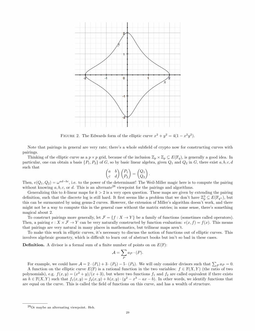
Figure 2. The Edwards form of the elliptic curve x2 + y2 = 4(1− x2y2).

Note that pairings in general are very rate; there’s a whole subfield of crypto now for constructing curves withpairings.

Thinking of the elliptic curve as a p× p grid, because of the inclusion Zp×Zp ⊆ E(Fq), is generally a good idea. Inparticular, one can obtain a basis P1, P2 of G, so by basic linear algebra, given Q1 and Q2 in G, there exist a, b, c, dsuch that (

a bc d

)(P1

P2

)=

(Q1

Q2

).

Then, e(Q1, Q2) = ωad−bc, i.e. to the power of the determinant! The Weil-Miller magic here is to compute the pairingwithout knowing a, b, c, or d. This is an alternate28 viewpoint for the pairings and algorithms.

Generalizing this to k-linear maps for k > 2 is a very open question. These maps are given by extending the pairingdefinition, such that the discrete log is still hard. It first seems like a problem that we don’t have Z3

p ⊆ E(Fqα), butthis can be surmounted by using genus-2 curves. However, the extension of Miller’s algorithm doesn’t work, and theremight not be a way to compute this in the general case without the matrix entries; in some sense, there’s somethingmagical about 2.

To construct pairings more generally, let F = f : X → Y be a family of functions (sometimes called operators).Then, a pairing e : X ×F → Y can be very naturally constructed by function evaluation: e(x, f) = f(x). This meansthat pairings are very natural in many places in mathematics, but trilinear maps aren’t.

To make this work in elliptic curves, it’s necessary to discuss the notion of functions out of elliptic curves. Thisinvolves algebraic geometry, which is difficult to learn out of abstract books but isn’t so bad in these cases.

Definition. A divisor is a formal sum of a finite number of points on on E(F):

A =∑P

aP · (P ).

For example, we could have A = 2 · (P1) + 3 · (P2)− 5 · (P3). We will only consider divisors such that∑P aP = 0.

A function on the elliptic curve E(F) is a rational function in the two variables: f ∈ F(X,Y ) (the ratio of twopolynomials), e.g. f(x, y) = (x2 + y)/(x+ 3), but where two functions f1 and f2 are called equivalent if there existsan h ∈ F(X,Y ) such that f1(x, y) = f2(x, y) + h(x, y) · (y2 − x3 − ax− b). In other words, we identify functions thatare equal on the curve. This is called the field of functions on this curve, and has a wealth of structure.

28Or maybe an alternating viewpoint. Heh.

29