Modular curves - math.purdue.edu

Chapter 2

Modular curves

2.1 The action of SL2(R)We let GL

2

(C) act on the Riemann sphere C [ {1} by fractional linear trans-formations ✓

a bc d

◆· ⌧ 7! a⌧ + b

c⌧ + d

Note that we can identify C[{1} = P1

C. With respect to this, the above actionof GL

2

(C) coincides with the usual action on the projective line by [v] 7! [Av].

Lemma 2.1.1. SL2

(R) acts transitively on the upper half plane H = {⌧ 2 C |Im ⌧ > 0} by fractional linear transformations. The stabilizer of i is SO(2).Therefore, we can identify H = SL

2

(R)/SO(2).

Proof. If

✓a bc d

◆2 SL

2

(R) and ⌧ 2 C, then

Ima⌧ + b

c⌧ + d=

Im ⌧

|c⌧ + d|2 (2.1)

This shows that SL2

(R) preserves H. We have

✓a bc d

◆· i = (ca+ db) + i

c2 + d2

It is now an easy exercise to see that given ⌧ 2 H, we can find a solution to

A · i = ⌧

with A 2 SL2

(R), and that if ⌧ = i, we must have A 2 SO(2).

We can view H as the upper hemisphere of the Riemann sphere P1

C. Theaction of SL

2

(R) extends to the boundary @H = P1

R = R [ {1}. In order to

12

better visualize the action, it useful to note that H has a Riemannian metric,called the hyperbolic or Poincare metric, where the geodesics are lines or circlesmeeting @H at right angles. The action of SL

2

(R) preserves this metric, so ittakes a geodesic to another geodesic.

2.2 The modular group SL2(Z)Let L

⌧

= Z+Z⌧ with ⌧ 2 H as before. We can see that elliptic curves E⌧

= C/L⌧

and E⌧

0 are isomorphic if and only if L⌧

= L⌧

0 .

Lemma 2.2.1.

(a) If (u, v)T , (u0, v0)T 2 B+, then Zu+ Zv = Zu0 + Zv0 if and only if (u, v)T

and (u0, v0)T lie in the same orbit of SL2

(Z).

(b) L⌧

= L⌧

0 if and only ⌧, ⌧ 0 lie in the same orbit under SL2

(Z).Proof. If Zu+Zv = Zu0 +Zv0, there would be change of basis matrix A taking(u, v)T to (u0, v0)T . A is necessarily integral with positive determinant, andthis already ensures that A 2 SL

2

(Z). The converse is easy. (b) follows from(a).

From this lemma, we can conclude that:

Theorem 2.2.2. The set of isomorphism classes of elliptic curves (over C) isparameterized by SL

2

(Z)\H.

At the moment, A1

= SL2

(Z)\H is just a set. In order to give more structure,we need to analyze the action more carefully. First observe that �I acts triviallyon H, so the action factors through � = PSL

2

(Z) = SL2

(Z)/{±I}. Considerthe closed region F ⇢ C bounded by the unit circle and the lines Im z = ±1/2depicted below.

TSF

F

SF

TFT−1

F

STF

Figure 2.1: Fundamental domain

Let S =

✓0 �11 0

◆, T =

✓1 10 1

◆. These act by z 7! �1/z and z 7! z + 1

respectively. S is a reflection about i which interchanges the regions |z| � 1 and|z| 1. They generate a subgroup G ✓ �.

13

Theorem 2.2.3.

(a) The union of translates gF , g 2 G, covers H.

(b) An interior point of F does not lie in any other translate of F under G.

(c) The isotropy group of z 2 F is trivial unless it is one of the points{i, e⇡i/3, e2⇡i/3} marked in the diagram. The isotropy group is hSi, hST i, hTSirespectively.

Proof. The intuition behind this can be understood from the picture. Repeat-edly applying S and T±1 to F gives a tiling of H by hyperbolic triangles. Choose⌧ 2 H, we want to find A0 2 SL

2

(Z) and ⌧ 0 2 F such that A0 · ⌧ 0 = ⌧ . Using(2.1), we can see that {ImA · ⌧ | A 2 SL

2

(Z)} has a maximum M . Choose anA which realizes this maximum. Choose an integer n so that ⌧ 0 = TnA⌧ hasreal part in [�1/2, 1/2]. Observe that Im ⌧ 0 = M . If |⌧ 0| < 1 then �1/⌧ 0 wouldhave imaginary bigger than M which is impossible. It follows that ⌧ 0 2 F , and⌧ lies in its orbit. This proves (a). For the remaining parts, see Serre [Se, pp79].

The set F is called a fundamental domain for the action of G. We can drawa number of useful conclusions.

Corollary 2.2.4. G = PSL2

(Z), i.e. S and T generate PSL2

(Z).

Proof. Let z 2 F be an interior point, and h 2 �. Then hz = gz for some g 2 G.Since z 2 h�1gF , we must have h�1g = I.

Corollary 2.2.5. The nontrivial elements of finite order in � are conjugate toS or (ST )±1.

Proof. A nontrivial element of finite must lie in the isotropy group of somepoint in H. The points in the plane with nontrivial isotropy groups must be atranslate of i or e2⇡i/3. Their isotropy groups must be conjugate to the isotropygroups of one these two points.

Corollary 2.2.6. The action of PSL2

(Z) is properly discontinuous, whichmeans that for every point p 2 H, there is a neighbourhood U such that gU\U =; for all but finitely many g.

We can give A1

the quotient topology where U ✓ A1

is open if and only itspullback to H, under the projection ⇡ : H ! A

1

is open.

Proposition 2.2.7. The topology on A1

is Hausdor↵. In fact, it is homeomor-phic to C

Proof. The first statement follows immediately from the last corollary. Usingthe above results, one can see that A

1

is obtained by gluing the two boundinglines of F and folding the circlular boundary in half. This is easily seen to behomeomorphic to the sphere minus the north pole.

14

A1

has a natural compactification A1

given by adding single point at infinityto make it a sphere. We will follow the convention of the automorphic formliterature and call it a cusp. It is important to keep in mind that this clasheswith the usual terminology in algebraic geometry, that a cusp is a singularityof the form y2 = x3. We will refer the last thing as cuspidal singularity inorder to avoid confusion. We can construct this a quotient as follows. LetH⇤ = H [ Q [ {1} ⇢ P1. The action of � on P1 stabilizes H⇤. On H itcoincides with the standard action, and on @H⇤ = Q [ {1} it consists of asingle orbit. Thus �\H⇤ = A

1

as a set. In order to get the correct topology onthe quotient, one needs a somewhat exotic topology of H⇤. On H it’s the usualone, but on @H⇤ a fundamental system of neighbourhoods of (a translate of) 1are (translates of) strips Im z > n, n 2 N.

2.3 Modular forms

Since A1

has a topology, we can talk about continuous functions on it. We cansee that f : A

1

! C is continuous if and only if it’s pullback ⇡⇤f := f � ⇡is continuous. Let us also declare that a function on an open subset of A

1

isholomorphic or meromorphic if its pullback to H has the same property. Thismeans that such functions correspond to �-invariant functions on H. Beforeconstructing nontrivial examples, we want to relax the condition. We say thatf is automorphic, with automorphy factor �

�

(z), if it satisfies the functionalequation

f(�z) = ��

(z)f(z)

This is very similar to what we did with theta functions. If we have two suchfunctions with the same factor, their ratio would be invariant. Note that forthis to work, we need to impose a consistency condition

��⇠

(z)f(z) = f(�⇠z)

= ��

(⇠z)f(⇠z) = ��

(⇠z)�⇠

(z)f(z)

Cancelling f , leads to a so called cocycle condition on the automorphy factor

��⇠

(z) = ��

(⇠z)�⇠

(z)

As the terminology suggests, ��

does give an element of a certain cohomologygroup. Rather than pursuing this direction, let us look for natural automorphicforms/factors in nature. Given a meromorphic di↵erential form ! = f(z)dz on

H, let us see how it transforms under � =

✓a bc d

◆2 SL

2

(Z). We can see that

! 7! f(� · z)d✓az + b

cz + d

◆= (cz + d)�2f(� · z)dz

15

We say that f(z) is a weakly modular form of weight 2, with respect to �, iff(z)dz is invariant. We say that f is weakly modular of weight 2k if it

f(z) = (cz + d)�2kf

✓az + b

cz + d

◆(2.2)

This means that the tensor f(z)dz⌦k is invariant. More generally, it makessense to consider weakly modular forms of arbitrary integer weight `, satisfying

f(z) = (cz + d)�`f

✓az + b

cz + d

◆

However, when ` is odd, taking � = �I, shows that f = �f , so it’s zero! Naturalnonzero examples do exist for other groups however, as we shall see shortly.

To drop the “weakly”, we impose holomorphy conditions on H but also atinfinity. To understand what the last part means, we first note that by using Sand T , (2.2) is equivalent to

f(z + 1) = f(z)

f(�1/z) = zkf(z)(2.3)

The first condition means that we have a Fourier expansion

f(z) =1X

�1an

e2⇡inz =1X

�1an

qn

where q = e2⇡iz. Note that as z ! i1, q ! 0. So we want to think of q as thelocal parameter at infinity. Then the Fourier series becomes the Laurent seriesin q. f is a modular form of weight 2k if it is holomorphic in H, (2.2) holds,and the Fourier coe�cients a

n

= 0 for n < 0. It is called a cusp form of weight2k if in addition a

0

= 0.

Theorem 2.3.1. The Eisenstein series

G2k

(z) =X

Z2�0

1

(mz + n)2k

is a modular form of weight 2k, when k � 2.

�(z) = (60G4

(z))3 � 27(140G6

(z))2

is a cusp form of weight 12.

Proof. The sum can be seen to converge uniformly on compact sets, so it mustconverge to a holomorphic function on H. One has

G2k

(az + b

cz + d) = (cz + d)2k

X 1

(ma+ ndc)z + (mb+ nd))2k

16

The vectors (ma + ndc,mb + nd) can be seen to run over Z2 � 0. So the rightside can be rewritten as

(cz + d)2kG2k

(z)

as required.We have to check holomorphy at infinity. By uniform convergence, we can

evaluate the limit as z ! 1 term by term. When m 6= 0, have (mz+n)�2k ! 0as z ! 1. Therefore

limz!1

G2k

(z) = 21X

n=1

1

n2k

= 2⇣(2k)

where ⇣ is the Riemann zeta function. Euler gave explicit formulas for the values

⇣(4) =⇡4

90

⇣(6) =⇡6

945

This allows us to evaluate limz!1 �(z) and check that it’s zero.

Corollary 2.3.2.

j(z) = 1728(60G

4

(z))3

�

is weakly modular of weight 0.

Finally, let us consider Jacobi’s theta function. This is a function of twovariables ✓(z, ⌧). We already studied the behaviour in the first, now we considerthe second where we set z = 0.

✓(0, ⌧) =X

n2Zexp(⇡in2⌧)

From this formula, we see that

✓(0, ⌧ + 2) = ✓(0, ⌧)

There is also a somewhat subtler functional equation.

Theorem 2.3.3. We have

✓(0,�1/⌧) =p�i⌧ ✓(0, ⌧)

where the complex square root needs to be handled with the usual care.

Sketch. We need the Poisson summation formula [DM], which tells us that

1X

n=�1f(n) =

1X

n=�1f(n)

17

where f is a rapidly decreasing smooth (aka Schwartz) function, and

f(v) =

Z 1

�1f(u)e�2⇡iuvdu

is its Fourier transform. The Fourier transform of the Gaussian e�⇡u

2⌧ is

⌧�1/2e�⇡v

2/⌧ . Therefore the Poisson summation formula shows that

T (1/y) =pyT (y)

where T (y) = ✓(0, iy). The theorem follows by analytic continuation.

Corollary 2.3.4.

✓(0,�1/⌧)2 = �i⌧✓(0, ⌧)2

The last equation plus the previous periodicity suggests that ✓(0, 1/⌧)2 is amodular form of some kind. In fact, it is a modular form of weight one for asubgroup �(4) to be defined below. See [MT, p 39].

2.4 Modular curves

With the topology of X(1) = A1

constructed earlier, which is homeomorphic toP1, we can construct a sheaf of functions O

X(1)

as follows. Let �(1) = SL2

(Z).Given a �(1)-invariant open set U ⇢ H, let us say that a holomorphic function fon it is modular of weight 2k if (2.2) holds and the negative Fourier coe�cients

vanish when 1 2 U . Given an open set U ⇢ X(1), let f 2 OX(1)

(U) be amodular form on the preimage ⇡�1U \ H of weight 0. We can view f as afunction on U , where the value at z 2 U � {1} is the value at any of thepreimages, and the value at 1 is the zeroth Fourier coe�cient.

Proposition 2.4.1. The ringed space (X(1),OX(1)

) is a Riemann surface.

Sketch. The key point is to show that any point x 2 X(1) has a neighbourhoodD with a homeomorphism z, called a local coordinate or parameter, to a diskin C, such that holomorphic functions on both disks coincide. There are threecases: x = 1, x is an image of one of the fixed points i, e2⇡i/3, or x is anyother point. The first case was essentially done in the last section, q is the localcoordinate at 1. The third case is straight forward. The map ⇡ : H ! X(1) isunramified over x A local coordinate z at a point y 2 H lying over x will give alocal coordinate at x. The map ⇡ is ramified at i and e2⇡i/3 with ramificationindex e = 2 and 3 respectively. ze will give a local coordinate at the image.

It is worth noting that the images of i and e2⇡i/3 are nonsingular, andtherefore no di↵erent from any other point from this point of view. However,these points clearly are special. One way to keep track of this, is the to use thelanguage of orbifolds or stacks. To simplify our story, we won’t do this here.

18

Given an integer N > 0, the principal congruence subgroup of level N of�(1) = SL

2

(Z) is

�(N) = ker�(1) ! SL2

(Z/N) = {M 2 �(1) | M ⌘ I mod N}A congruence group is a subgroup of �(1) containing some �(N). It thereforehas finite index in �(1). Some other important examples are

�1

(N) = {M 2 �(1) | M ⌘✓1 ⇤0 1

◆mod N}

�0

(N) = {M 2 �(1) | M ⌘✓⇤ ⇤0 ⇤

◆mod N}

We have inclusions�(N) ⇢ �

1

(N) ⇢ �0

(N) ⇢ �(1)

We can compute the indices.

Proposition 2.4.2.

(a)

[�(1) : �(N)] = N3

Y✓1� 1

p2

◆

where p runs over primes dividing N .

(b)

[�(1) : �1

(N)] = N2

Y✓1� 1

p2

◆

(c)

[�(1) : �0

(N)] = NY✓

1 +1

p

◆

Proof. We have [�(1) : �(N)] = |SL2

(Z/N)|, [�1

(N) : �(N)| = |Z/N | and[�

0

(N),�1

(N)] = |(Z/N)⇤|. These can be checked to yield the above formulas.

Lemma 2.4.3. �(N) is torsion free once N � 3.

Given such a group, it will act on H⇤, let Y (�0) = �0\H and let X(�0) =�0\H⇤. The points of X(�0)�Y (�0) are called cusps. We write Y (N), Y

1

(N) etc.when the groups are �(N),�

1

(N). A meromorphic function f on H is weaklymodular form of weight 2k, with respect to �0, if (2.2) holds for matrices in �0.

The isotropy group of 1 is a finite index subgroup of h✓1 10 1

◆i so it is of the

form h✓1 n0 1

◆i for some n. This implies that a weakly modular form satisfies

f(z + n) = f(z)

19

So that it has a Fourier expansion in q = e2⇡iz/n. A similar Fourier expansionoccurs at all the other cusps. We say that f is a modular (resp. cusp) form ifit is holomorphic in H and the negative (resp. nonpositive) Fourier coe�cientsat each cusp vanish. When extend this to the case where the domain of f isan invariant open set. Then we can turn Y (�0) ⇢ X(�0) into Riemann surfacesexactly as above. These are called modular curves. We have a holomorphic map

X(�0) ! X(�(1)) = A1

⇠= P1

induced by inclusion �0 ⇢ �(1). This is a branched covering. So we can computethe genus using the Riemann-Hurwitz formula, which says that if Y ! X is adegree d branched covering of compact Riemann surfaces of genus g(Y ) andg(X), then

2g(Y )� 2 = (2g(X)� 2)d+X

y2Y

(ey

� 1)

where ey

is the ramification index which counts the number of sheets which“come together” at y. We will use this to compute for most of the principalcongruence groups. More general formulas can be found in [DS, S].

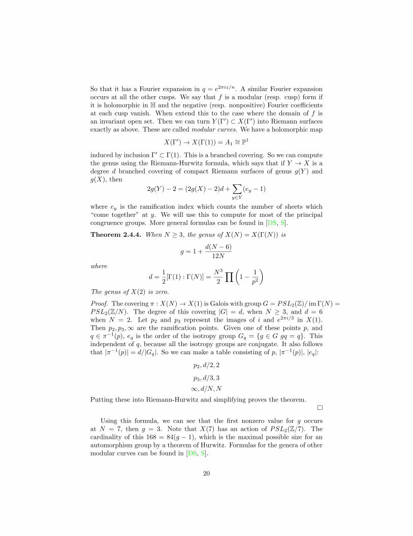
Theorem 2.4.4. When N � 3, the genus of X(N) = X(�(N)) is

g = 1 +d(N � 6)

12N

where

d =1

2[�(1) : �(N)] =

N3

2

Y✓1� 1

p2

◆

The genus of X(2) is zero.

Proof. The covering ⇡ : X(N) ! X(1) is Galois with groupG = PSL2

(Z)/ im�(N) =PSL

2

(Z/N). The degree of this covering |G| = d, when N � 3, and d = 6when N = 2. Let p

2

and p3

represent the images of i and e2⇡i/3 in X(1).Then p

2

, p3

,1 are the ramification points. Given one of these points p, andq 2 ⇡�1(p), e

q

is the order of the isotropy group Gq

= {g 2 G gq = q}. Thisindependent of q, because all the isotropy groups are conjugate. It also followsthat |⇡�1(p)| = d/|G

q

|. So we can make a table consisting of p, |⇡�1(p)|, |eq

|:p2

, d/2, 2

p3

, d/3, 3

1, d/N,N

Putting these into Riemann-Hurwitz and simplifying proves the theorem.

Using this formula, we can see that the first nonzero value for g occursat N = 7, then g = 3. Note that X(7) has an action of PSL

2

(Z/7). Thecardinality of this 168 = 84(g � 1), which is the maximal possible size for anautomorphism group by a theorem of Hurwitz. Formulas for the genera of othermodular curves can be found in [DS, S].

20

2.5 Dimension of spaces of modular forms

Given a smooth curve X and a divisor D, let ⌦1

X

(D) = ⌦1

X

⌦OX

(D). It can beidentified with O

X

(K+D), where K is a canonical divisor. The space of globalsections �(X,⌦1

X

(D)) can be identified with the space of meromorphic 1-forms! satisfying div! +D � 0.

Theorem 2.5.1. Suppose that �0 is a torsion free congruence group. Let X =X(�0) and let D =

Ppi

be the sum of cusps. The space weight 2k modular forms(resp. cusp forms) M

2k

(�0) (resp. S2k

(�0)) is isomorphic to �(X,O(kK+kD))(resp. �(X,O(kK + (k � 1)D)). In particular, S

2

(�0) ⇠= �(X,⌦1

X

)

Proof. Let f(z) 2 M2k

(�0). Then f(z)(dz)⌦k is a �0-invariant holomorphicsection of (⌦1

H)⌦k, so it descends to a holomorphic section of (⌦1

Y (�

0)

)⌦k. We

have to check what happens near a cusp. We have a local coordinate q = e2⇡iz/n.By assumption f can be expanded as

P10

am

qm, with a0

= 0 for a cusp form.We have dz = (n/2⇡i)dq/q. So

f(z)(dz)⌦k =⇣ n

2⇡i

⌘k

(a0

q�k + a1

q1�k + . . .)dq⌦k

So the theorem follows.

Corollary 2.5.2. Suppose that X has genus g with m cusps, then

dimS2k

(�0) =

(g if k = 1

(2k � 1)(g � 1) + (k � 1)m if k > 1

Proof. The first case is an immediate consequence of the theorem. For thesecond, we use Riemann-Roch.

h0(O(kK + (k � 1)D)) = h0(O(kK + (k � 1)D))� h0(O((1� k)K � (k � 1)D)

= deg(kK + (k � 1)D) + 1� g

A product of a modular form of weight 2k and 2` is clearly a modular formof weight 2(k + `). Therefore

Lk

S2k

(�0) is a graded C-algebra.

Corollary 2.5.3. The algebra of modular forms is finitely generated.

Proof. This follows from the standard fact that the algebraM

k

H0(X,O(kE))

is finitely generated, whenever X is a compact Riemann surface and E is divisorwith degE � 0.

We refer to [DS, S] for more general formulas allowing k to be odd and �0 tohave torsion. Using these formulas, one can show that the algebra of modularforms for SL

2

(Z) is generated by the Eisenstein series G4

and G6

.

21

2.6 Moduli interpretation

As we saw, Y (1) parameterizes elliptic curves. While it’s intuitively clear whatthis means, the actual statement requires a bit more precision. Let us define ananalytic family of (compact) complex manifolds to be a (proper) holomorphicsubmersion of complex manifolds f : E ! B. We recall that a submersion ismap such that derivative is surjective on tangent spaces. This implies that fibresE

b

= f�1(b) are complex submanifolds. By an analytic family of elliptic curveswe mean an analytic family of compact complex manifolds f : E ! B with aholomorphic section s : B ! E such that each fibre E

b

is a compact Riemannsurface of genus one. We can regard E

b

as an elliptic curve with origin s(b).

Theorem 2.6.1. Y (1) has the following properties:

(a) The map E ! j(E) gives a bijection between the set of isomorphismclasses of elliptic curves over C and points of Y (1),

(b) Given an analytic family elliptic curves E ! B, the map B ! Y (1), calledthe classifying map, given by b 7! j(E

b

) is holomorphic.

The statement can be strengthened to completely characterize Y (1), but weneed a bit of terminology. Let Ellan(B) be the set of isomorphism classes ofanalytic families of elliptic curves over B, where isomorphism has the obviousmeaning. Given a holomorphic map B0 ! B, the pullback E 7! E ⇥

B

B0

gives a map Ellan(B) ! Ell(B0) which makes it into a contravariant functor.More generally, let M(�) be contravariant functor from the category of complexmanifolds (or schemes or...) to sets; one thinks of elements of M(B) as familiesof objects over B of interest. We say that M is representable by U , or that U isa fine moduli space for M , if there is a natural isomorphism of functors

M(B) ⇠= Hom(B,U)

Yoneda’s lemma, in category theory, tells us that U is completely determinedby this property, and moreover it carries a universal family such that any objectin M(B) is the pullback of it under some map B ! U . Although this is idealscenario for any moduli problem, it fails for Ellan. This is because there existsnontrivial families in Ellan(B) with constant j-invariant. Here is a generalconstruction.

Example 2.6.2. Let E be either Ei

or Eexp(2⇡i/3)

Either curve has a nontrivial

automorphism group G, which is cyclic in both cases. Choose a manifold B onwhich G acts freely, e.g. C⇤. The quotient (E ⇥ B)/G ! B/G is a nontrivialfamily with constant j-invariant.

In spite of this bad news, we do have a natural transformation Ellan(B) !Hom(B, Y (1)), which is universal in an appropriate sense, and which inducesa bijection when B is a point. We say that Y (1) is the coarse moduli space forEllan.

22

The other modular curves have similar interpretations. Let us explain thecharacterizations of Y (N) = Y (�(N)) in a somewhat informal way. GivenE

⌧

= C/Z + Z⌧ , the image of ( 1

N

, ⌧

N

) gives a basis for the N -torsion points inE

⌧

. We refer to this as a level N -structure. If A 2 �(N), then the inducedisomorphism E

⌧

⇠= EA·⌧ takes the above level N -structure of the first curve to

the level structure of the second. In order to make this notion independent ofour representation of E

⌧

as a quotient, we note that the lattice is isomorphicto homology L

⌧

⇠= H1

(E⌧

,Z). Thus a level N -structure is a choice of basis forH

1

(E,Z/NZ) = H1

(E,Z) ⌦ Z/NZ, but not just any basis. The group carriesan intersection pairing

H1

(E,Z/N)⇥H1

(E,Z/NZ) ! Z/N

So now we can say that a level N -structure is a basis for H1

(E,Z/NZ) whichis symplectic in the sense that the matrix of the above pairing is

✓0 1�1 0

◆

Theorem 2.6.3. Y (N) is the coarse moduli space of elliptic curves with levelN -structure. When N � 3 it is a fine moduli space.

Recall that the assumptionN � 3 is precisely the condition to guarantee that�(N) is torsion free. This same condition also allows us to kill the automorphismgroups which created the problem in example 2.6.2.

For the other moduli spaces, we have similar interpretations. Y1

(N) =Y (�

1

(N)) is the coarse moduli space of pairs (E,P ) consisting of an ellipticcurve E and a point P of order N . Y

0

(N) is the moduli space of pairs (E,C)consisting of an elliptic curve and a cyclic subgroup of the group of N -torsionpoints. The projections

Y (N) ! Y1

(N) ! Y0

(N) ! Y (1)

induced by the inclusions

�(N) ⇢ �1

(N) ⇢ �0

(N) ⇢ �

have moduli interpretations. Given E a level N -structure is a pair of N -torsionpoints P,Q satisfying suitable conditions. The map Y (N) ! Y

1

(N) correspondsto the forgetful map (E,P,Q) 7! (E,P ).

2.7 Models over number fields

So far we have considered modular curves as Riemann surfaces, but in fact theyare algebraic curves. This is true of any compact Riemann surface minus a finiteset of points. However, a more natural way to see this is to consider algebraicversions of the moduli problems consider earlier. As a bonus this will show

23

that these curves are naturally defined over number fields and even over ringsof integers. This is very important for applications to number theory. Let usstart with Y (1). We consider the corresponding moduli problem in the algebraicsetting. Given a scheme B, an elliptic curve over it is a smooth proper map isa smooth proper map f : E ! B , with a section, such that the closed fibres off are genus one curves. Let Ell(B) denote the isomorphism classes of ellipticcurves over B. Then Y (1)Z = SpecZ[j] is a coarse moduli scheme for Ell(�),and this gives a model for Y (1) over the integers, i.e. Y (1) is the complexmanifold associated to Y (1)Z ⇥

SpecZ SpecC.Next let us turn to Y (N). We can formulate the definition of level structure

of an elliptic curve over an arbitrary field k. In this case, we need N to beprime to the characteristic. Then a level N -structure is a pair of N -torsionpoints P,Q 2 E(k) such that they generate the group of N -torsion points andsuch that e

N

(P,Q) is a primitive N -root of unity. Here eN

is the Weil pairingwhose definition can be found in [Si]. Note that the condition forces k to containa primitive N -root of unity. More generally, there is a notion of a level structurefor an elliptic curve over a base scheme. This is basically a pair of sections whichinduces a level structure on the closed fibres.

Theorem 2.7.1. There exists a scheme Y (N) defined over Z[1/N, e2⇡i/N ] whichis the coarse moduli space of elliptic curves with level N -structure. It is a finemoduli when N � 3. The set of complex points is the Riemann surface �(N)\Hconsidered before.

See Deligne-Rapoport [DR] for the construction in general. They also give amore general construction which would include the Y

i

(N). Y0

(N) is particularlyinteresting because it is defined over Q. When N is small, Y (N) can be madevery explicit. We have

Y (2) = SpecZ[t,1

t(t� 1)]

Although this is not fine, there is an “almost” universal family called the Leg-endre family

y2z = x(x� z)(x� tz)

in P2

Z. Over a field, this curve has 4 branch points over 0, 1, t,1. Take the firstto be the origin, and the next two to be the level 2-structure.

When N = 3, let R = Z[1/3, e2⇡i/3], then

Y (N) = SpecR[t,1

t3 � 1]

The universal family is given by the elliptic curve

x3 + y3 + z3 = 3txyz

in P2

R

with section [1,�1, 0]. The level 3-structure is given by the sections[�1, 0, 1] and [�1, e2⇡i/3, 0].

24