Credit Risk Evaluation

Credit Risk Evaluation Modeling – Analysis – Management

INAUGURAL-DISSERTATION ZUR ERLANGUNG DER WÜRDE EINES DOKTORS

DER WIRTSCHAFTSWISSENSCHAFTEN DER WIRTSCHAFTSWISSENSCHAFTLICHEN FAKULTÄT DER RUPRECHT-KARLS-UNIVERSITÄT HEIDELBERG

VORGELEGT VON UWE WEHRSPOHN

AUS EPPINGEN

HEIDELBERG, JULI 2002

2

This monography is available in e-book-format at http://www.risk-and-evaluation.com. This monography was accepted as a doctoral thesis at the faculty of economics at Heidelberg University, Ger-many. © 2002 Center for Risk & Evaluation GmbH & Co. KG Berwanger Straße 4 D-75031 Eppingen www.risk-and-evaluation.com

3

Acknowledgements My thanks are due to Prof. Dr. Hans Gersbach for lively discussions and many ideas that con-

tributed essentially to the success of this thesis.

Among the many people who provided valuable feedback I would particularly like to thank

Prof. Dr. Eva Terberger, Dr. Jürgen Prahl, Philipp Schenk, Stefan Lange, Bernard de Wit,

Jean-Michel Bouhours, Frank Romeike, Jörg Düsterhaus and many colleagues at banks and

consulting companies for countless suggestions and remarks. They assisted me in creating the

awareness of technical, mathematical and economical problems which helped me to formulate

and realize the standards that render credit risk models valuable and efficient in banks and

financial institutions.

Further, I gratefully acknowledge the profound support from Gertrud Lieblein and Computer

Sciences Corporation – CSC Ploenzke AG that made this research project possible.

My heartfelt thank also goes to my wife Petra for her steady encouragement to pursue this

extensive scientific work.

Uwe Wehrspohn

4

Introduction

In the 1990ies, credit risk has become the major concern of risk managers in financial institu-

tions and of regulators. This has various reasons:

• Although market risk is much better researched, the larger part of banks’ economic

capital is generally used for credit risk. The sophistication of traditional standard

methods of measurement, analysis, and management of credit risk might, there-

fore, not be in line with its significance.

• Triggered by the liberalization and integration of the European market, new chan-

nels of distribution through e-banking, financial disintermediation, and the en-

trance of insurance companies and investment funds in the market, the competitive

pressure upon financial institutions has increased and led to decreasing credit mar-

gins1. At the same time, the number of bankruptcies of companies stagnated or in-

creased2 in most European countries, leading to a post-war record of insolvencies

in 2001 in Germany3.

• A great number of insolvencies and restructuring activities of banks were influ-

enced by prior bankruptcies of creditors. In the German market, prominent exam-

ples are the Bankgesellschaft Berlin (2001), the Gontard-MetallBank (2002), the

Schmidtbank (2001), and many mergers among regional banks4 to avoid insol-

vency or a shut down by regulatory authorities.

The thesis contributes to the evaluation and development of credit risk management methods.

First, it offers an in-depth analysis of the well-known credit risk models Credit Metrics (JP

Morgan), Credit Risk+ (Credit Suisse First Boston), Credit Portfolio View (McKinsey &

Company) and the Vasicek-Kealhofer-model5 (KMV Corporation). Second, we develop the

Credit Risk Evaluation model6 as an alternative risk model that overcomes a variety of defi-

ciencies of the existing approaches. Third, we provide a series of new results about homoge-

nous portfolios in Credit Metrics, the KMV model and the CRE model that allow to better

1 Bundesbank (2001). 2 Creditreform (2002), p. 4. 3 Creditreform (2002), p. 16. 4 Between 1993 and 2000 1,000 out of 2,800 Volks- und Raiffeisenbanken and 142 out of 717 savings banks ceased to

exist in Germany (Bundesbank 2001, p. 59). All of them merged with other banks so that factual insolvency could be avoided in all cases. Note that shortage of regulatory capital in consequence of credit losses was not the reason for all of these mergers. Many of them were motivated to achieve cost reduction and were carried out for other reasons.

5 We refer to the Vasicek-Kealhofer-model also as the KMV model. 6 Credit Risk Evaluation model is a trademark of the Center for Risk & Evaluation GmbH & Co. KG, Heidelberg. We re-

fer to the Credit Risk Evaluation model also as the CRE model.

5

understand and compare the models and to see the impact of modeling assumptions on the

reported portfolio risk. Fourth, the thesis covers all methodological steps that are necessary to

quantify, to analyze and to improve the credit risk and the risk adjusted return of a bank port-

folio.

Conceptually, the work follows the risk management process that comprises three major as-

pects: the modeling process of the credit risk from the individual client to the portfolio (the

qualitative aspect), the quantification of portfolio risk and risk contributions to portfolio risk

as well as the analysis of portfolio risk structures (the quantitative aspect), and, finally, meth-

ods to improve portfolio risk and its risk adjusted profitability (the management aspect).

The modeling process

The modeling process includes the identification, mathematical description and estimation of

influence factors on credit risk. On the level of the single client these are the definitions of

default7 and other credit events8, the estimation of default probabilities9, the calculation of

credit exposures10 and the estimation of losses given default11. On the portfolio level, depend-

encies and interactions of clients need to be modeled12.

The assessment of the risk models is predominantly an analysis of the modeling decisions

taken and of the estimation techniques applied. We show that all of the four models have con-

siderable conceptual problems that may lead to an invalid estimation, analysis and pricing of

portfolio risk.

In particular, we identify that the techniques applied for the estimation of default probabilities

and related inputs cause systematic errors in Credit Risk+13 and Credit Portfolio View14 if

certain very strict requirements on the amount of available data are not met even if model

assumptions are assumed to hold. If data is sparse, both models are prone to underestimate

default probabilities and in turn portfolio risk.

For Credit Metrics and the KMV model, it is shown that both models lead to correct results if

they are correctly specified. The concept of dependence that is common to both models –

called the normal correlation model – can easily be generalized by choosing a non-normal

7 See section I.A. 8 I.e. of rating transitions, see sections I.B.4, I.B.6.c)(4), I.B.7. 9 See section I.B. 10 Section I.C. 11 Section I.D. 12 See Section II.A. 13 Section I.B.5 14 Section I.B.6

6

distribution for joint asset returns. As one of the main results, we prove for homogenous port-

folios that the normal correlation model is precisely the risk minimal among of all possible

generalizations of this concept of dependence. This implies that even if the basic concept of

dependence is correctly specified, Credit Metrics and the Vasicek-Kealhofer model systemati-

cally underestimate portfolio risk if there is any deviation from the normal distribution of as-

set returns.

Credit Risk+ has one special problem regarding the aggregation of portfolio risk15. It is the

only model whose authors intend to avoid computer simulations to calculate portfolio risk and

attain an analytical solution for the portfolio loss distribution. For this reason, the authors

choose a Poisson approximation of the distribution of the number of defaulting credits in a

portfolio segment. As a consequence each segment contains an infinite number of credits.

This hidden assumption may lead to a significant overestimation of risk in small segments,

e.g. when the segment of very large exposures in a bank portfolio is considered that is usually

quite small. Thus, Credit Risk+ is particularly suited for very large and homogenous portfo-

lios. However, at high percentiles, the reported portfolio losses even always exceed the total

portfolio exposure.

With the Credit Risk Evaluation model, we present a risk model that avoids these pitfalls and

integrates a comprehensive set of influence factors on an individual client’s risk and on the

portfolio risk. In particular, the CRE model captures influences on default probabilities and

dependencies such as the level of country risk, business cycle effects, sector correlations and

individual dependencies between clients. This leads to an unbiased and more realistic estima-

tion of portfolio risk16.

The CRE model also differs from the other models with respect to the architecture, which is

modular in contrast to the monolithic design in other models. This means that the corner-

stones of credit risk modeling such as the description of clients’ default probabilities, expo-

sures, losses given default, and dependencies are designed as building blocks that interact in

certain ways, but the methods in each module can be exchanged and adjusted separately. This

architecture has the advantage that, by choosing appropriate methods in each component, the

overall model may be flexibly adapted to the type and quality of the available data and to the

structure of the portfolio to be analyzed.

15 Section II.A.3.a) 16 Sections I.B.7 and II.A.2

7

For instance, if the portfolio is large and if sufficiently long histories of default data are avail-

able, business cycle effects on default probabilities can be assessed in the CRE model. Other-

wise, more simple methods to estimate default can be applied such as long term averages of

default frequencies etc. Similarly, country risk typically is one of the major drivers of portfo-

lio risk of internationally operating banks. In turn, these banks should use a risk model that

can capture its effect17. Regional banks, on the other hand, might not have any exposures on

an international scale and, therefore, may well ignore country risk.

Moreover, an object-oriented software implementation of the model can directly follow its

conceptual layout. Here, building blocks translate into classes and methods into routines

within the classes. This makes it easy to adapt the software to the model and to integrate new

methods.

It is worth noting that the CRE model contains Credit Metrics and the Vasicek-Kealhofer

model as special cases, if methods in the modules are appropriately specified.

The presentation of our analyses and results follows the modular architecture of the CRE

model. We go through the building blocks separately and only analyze the respective compo-

nent of each model and, if necessary, the restrictions that the choice of a particular model in

one building block imposes upon other components. This structure renders it possible to as-

sess each method in each module individually and to avoid that errors accumulate or offset

each other and make the resulting effect intransparent and difficult to apprehend.

Analysis of portfolio risk structures

After all components of a portfolio model are defined and all relevant input parameters are

estimated, the next step in the credit risk management process entails the quantification of

portfolio risk and of risk contributions to portfolio risk and the analysis of portfolio risk struc-

tures. This step is entirely based upon the portfolio loss distribution and on the concept of

marginal risks. As they are based upon standardized model outputs, all methods to analyze

risk structures are generally valid and independent of the underlying risk model.

We develop a general simulation based approach how the portfolio loss distribution and the

expected loss, the standard deviation, the value at risk, and the shortfall as specific risk meas-

ures can be estimated and supply formulas for confidence intervals around the estimated risk

measures and confidence bands around the loss distribution. We also show that the calculation

17 Sections I.B.7.a)(1) and II.A.5.

8

of value at risk and shortfall may be subject to systematic estimation errors if the number of

simulation runs is not sufficiently large with regard to the required confidence level.

The mere calculation of risk measures for the entire portfolio and portfolio segments is usu-

ally not sufficient in order to capture the complexity of real world portfolio structures and to

localize segments where the risk manager has to take actions. This is due to the fact that dif-

ferent aspects of risk such as segments’ losses given default, their risk contributions, risk ad-

justed returns etc. may lead to very different pictures of the portfolio structure and may also

interact. I.e. a portfolio segment, that appears to be moderately risky if single aspects of risk

are considered in isolation, can gain a high priority if various concepts of risk and return are

evaluated in combination. For this reason, we give an example of a comprehensive portfolio

analysis and the visualization of portfolio risk in a ‘risk management cockpit’.

A complementary approach to improve portfolio quality that does not depend upon the actual

portfolio composition is algorithmic portfolio optimization. We develop a method that mini-

mizes portfolio shortfall under certain side-constraints such as the size of expected returns or

non-negativity of exposures and give an example of an optimization and its effect upon port-

folio composition and marginal risk contributions.

Risk management techniques

When portfolio risk is modeled, measured and decomposed, the risk manager may want to

take action to adjust the portfolio along value at risk, shortfall and return considerations. On

the level of the single client this can be done by adequate, risk adjusted pricing of new credits

and the allocation of credit lines. On the portfolio level, the allocation of economic capital as

well as the setting of risk, exposure and concentration limits, credit production guidelines, and

credit derivatives can be used, for instance, to redirect the portfolio.

The thesis is organized as follows: In the first part, we discuss the credit risk management of a

single client. This includes the modeling and estimation of clients’ risk factors and mainly the

risk adjusted pricing of financial products. In the second part, the focus is on the risk man-

agement of multiple clients. We begin with a detailed description and analysis of various con-

cepts of dependence between clients. Subsequent sections deal with the quantification and

analysis of portfolio risk and with risk management techniques.

9

Introduction 4

The modeling process 5

Analysis of portfolio risk structures 7

Risk management techniques 8

I. The credit risk of a single client 16

A. Definitions of default 16

B. Estimation of default probabilities 17

1. Market factor based estimation of default probabilities: the Merton model 17

a) Main concept 18 b) Assumptions 18 c) Derivation of default probability 20 d) Discussion 22

2. Extensions of Merton’s model by KMV 25

a) Discussion 26

3. Market factor based estimation of default probabilities: the Jarrow-Turnbull models 27

a) Main concept 27 b) Discussion 29

4. Rating based estimation of default probabilities: the mean value model 30

a) Main concept 30 b) Derivation of default probability 31 c) Discussion 32 d) How many rating categories should a financial institution distinguish? 39

5. Rating based estimation of default probabilities: Credit Risk + 40

a) Main concept 41 b) Derivation of default probability 41 c) Discussion 42

Table of contents

10

6. Rating based estimation of default probabilities: Credit Portfolio View 45

a) Main concept 45 b) Derivation of default probability 47 c) Discussion 49

(1) Modeling of macroeconomic processes 49 (2) Relation of default rates to systematic factors 50 (3) Example 53 (4) Conditional transition matrices 60 (5) Example 61 (6) Conclusion 63

7. Rating based estimation of default probabilities: the CRE model 64

a) Main concept and derivation of default probability 64 (1) Country risk 64 (2) Micro economic influences on default risk 66 (3) Macroeconomic influences on default risk 68 (4) Example 71 (5) Conditional transition probabilities 75

C. Exposures 76

a) Roles of counterparties 76 b) Concepts of exposure 77

(1) Present value 78 (2) Current exposure 78 (3) Examples 79 (4) Potential exposure 80 (5) Potential exposure of individual transactions or peak exposure 80 (6) Examples 80 (7) Potential exposure on a portfolio level 82 (8) Example 83 (9) Mean expected exposure 85 (10) Maximum exposure 86 (11) Artificial spread curves 86

c) Overview over applications 87

D. Loss and Recovery Rates 87

1. Influence factors 88

2. Random Recoveries 89

3. Practical problems 91

11

E. Pricing 91

1. Pricing of a fixed rate bond 91

2. Pricing of a European option 97

3. Equity allocation 98

II. The credit risk of multiple clients 101

A. Concepts of dependence 101

1. The normal correlation model 103

a) The Vasicek-Kealhofer model 103 b) Credit Metrics 106 c) Homogenous Portfolios 107

2. The generalized correlation model (CRE model) 112

a) Homogenous Portfolios 119 (1) Portfolio loss distribution 120 (2) Portfolio loss density 126 (3) Comparison of the normal and the generalized correlation model 129 (4) More complex types of homogenous portfolios 133 (5) Speed of convergence 137

b) Estimation of risk index distributions 139 c) Copulas 142

3. Random default probabilities (Credit Risk+ and Credit Portfolio View) 144

a) Credit Risk+ 144 b) Credit Portfolio View 146

4. A brief reference to the literature and comparison of the models applied to homogenous portfolios 146

5. Event driven dependencies (CRE model) 149

B. Time horizons for risk calculations 152

1. A standardized time horizon 152

2. Heterogeneous time horizons 155

C. Quantification of portfolio risk 155

1. Portfolio loss distribution 155

2. Expected loss 161

12

a) Estimation 161 b) Confidence intervals 162

3. Standard deviation 163


4. Value at risk 168

5. Shortfall 171


D. Risk analysis and risk management 173

1. Marginal risks 174

a) Marginal risks conditional to default 174 b) Marginal risks prior to default 175 c) Combinations of exposure and marginal risk 178 d) Expected risk adjusted returns 179 e) Summary 182

2. Credit derivatives 183

3. Portfolio optimization 183

a) Optimization approach 184 b) A portfolio optimization 185

Conclusion 188

Literature 189

13

List of figures Figure 1: Default probability vs. distance to default in Merton’s model .................................24 Figure 2: Deviation of portfolio value at risk dependent on number of rating categories .......34 Figure 3: Distributions of estimated default probabilities in mean value model......................36 Figure 4: Variance of mean value estimator of default probability..........................................38 Figure 5: Frequency of invalid volatility estimations in Credit Risk +....................................43 Figure 6: Bias of estimated default rate volatility in Credit Risk + dependent on number of

periods and number of clients...........................................................................................44 Figure 7: Bias of estimated default rate volatility in Credit Risk + dependent on number of

periods ..............................................................................................................................45 Figure 8: Observed and estimated default frequencies in the German economy 1976-1992...46 Figure 9: Persistence of macroeconomic shocks in Credit Portfolio View..............................50 Figure 10: Logit and inverse logit transformation....................................................................51 Figure 11: Convex transforms and probability distributions....................................................51 Figure 12: Bias of long-term mean default probability in Credit Portfolio View ....................54 Figure 13: Relative error of estimated long-term mean default probability in Credit Portfolio

View..................................................................................................................................54 Figure 14: Bias of estimated regression parameter β0 in Credit Portfolio View......................55 Figure 15: Standard deviation of estimated regression parameter 0β in Credit Portfolio View

..........................................................................................................................................56 Figure 16: Bias of estimated regression parameter β1 in Credit Portfolio View......................56 Figure 17: Standard deviation of estimated regression parameter β1 in Credit Portfolio View

..........................................................................................................................................57 Figure 18: Distributions of estimated parameter values for (β0,β1) in Credit Portfolio View..58 Figure 19: Distributions of long-term mean probabilities of default of estimated processes in

Credit Portfolio View .......................................................................................................59 Figure 20: Conditional and unconditional cumulative default probabilities in Credit Portfolio

View..................................................................................................................................63 Figure 21: Expected values of estimated parameter β0 in the CRE model under correlated

defaults..............................................................................................................................71 Figure 22: Standard deviation of estimated parameter β0 in the CRE model under correlated

defaults..............................................................................................................................72 Figure 23: Expected value of macro parameter β1 in the CRE model under correlated defaults

..........................................................................................................................................72 Figure 24: Standard deviation of estimated parameter β1 in the CRE model under correlated

defaults..............................................................................................................................73 Figure 25: Standard deviation of estimated parameters (β0,β1) in the CRE model dependent on

the size of correlations......................................................................................................73 Figure 26: Distributions of estimated parameter values (β0,β1) in the CRE model under

various correlations...........................................................................................................74 Figure 27: Add-on factor of a portfolio of options on 100 different shares .............................84 Figure 28: Potential exposure of a portfolio of options on 100 different shares ......................85 Figure 29: Beta distributions of recovery rates of public bonds in different seniority classes.89 Figure 30: Portfolio analysis, CAD, and equity allocation.......................................................99 Figure 31: Risk premiums, correlations, portfolio analysis, and regulatory capital

requirements ...................................................................................................................100 Figure 32: Default rates of corporates in Germany for different rating grades......................102 Figure 33: Abstract default threshold for a firm with annual probability of default of 1% ...104 Figure 34: Simulated bivariate normal distributions and marginals.......................................105

14

Figure 35: Loss distributions of homogenous portfolios in the normal correlation model 1 .110 Figure 36: Loss distributions of homogenous portfolios in the normal correlation model 2 .112 Figure 37: An empirical long tail distribution in finance: DAX-returns................................113 Figure 38: Spherical and elliptical distributions.....................................................................114 Figure 39: Densities of normal variance mixture distributions ..............................................117 Figure 40: Tail behavior of normal mixture distributions ......................................................118 Figure 41: Portfolio loss distributions in the generalized correlation model based on finite

mixture distributions.......................................................................................................122 Figure 42: Portfolio loss distributions in the generalized correlation model based on normal

inverse Gaussian distributions ........................................................................................123 Figure 43: Loss distributions resulting from uncorrelated Student-t-distributed risk indices 124 Figure 44: Loss distributions resulting from uncorrelated finite mixture distributed risk

indices.............................................................................................................................125 Figure 45: Portfolio loss densities in the bimixture correlation model ..................................127 Figure 46: Portfolio loss densities in the normal correlation model.......................................128 Figure 47: Trimodal portfolio loss densities in the trimixture correlation model ..................128 Figure 48: The low correlation effect in the finite mixture model .........................................129 Figure 49: Portfolio loss distributions in the normal versus the generalized correlation model

........................................................................................................................................130 Figure 50: Portfolio densities in the normal and the generalized correlation model..............131 Figure 51: Loss distribution of an almost homogenous portfolio in the NIG correlation model

........................................................................................................................................137 Figure 52: The speed of convergence towards the asymptotic portfolio loss distribution in the

generalized correlation model ........................................................................................139 Figure 53: Bivariate distributions with standard normal marginals and different copulas ....143 Figure 54: Loss distribution of a junk bond portfolio according to Credit Risk+..................145 Figure 55: Loss distributions resulting from Credit Risk+, Credit Portfolio View and the

normal correlation model................................................................................................148 Figure 56: Relative deviation of the portfolio loss distributions............................................148 Figure 57: The event risk effect in portfolio risk calculations: country risk ..........................150 Figure 58: Cascading effect of microeconomic dependencies ...............................................151 Figure 59: Influence of the time horizon on the 99.9%-value at risk.....................................153 Figure 60: Term structure of default rates: direct estimates versus extrapolated values........154 Figure 61: Uniform 95%-confidence bands for the portfolio loss distribution dependent on the

number of simulation runs..............................................................................................156 Figure 62: Pointwise 95%-confidence intervals for the portfolio loss distribution dependent on

the number of simulation runs ........................................................................................157 Figure 63: Accuracy of the estimation of the expected portfolio loss dependent on the number

of simulation runs ...........................................................................................................163 Figure 64: The ratio of value at risk and standard deviation of credit portfolios ...................165 Figure 65: Accuracy of the estimation of the standard deviation of portfolio losses dependent

on the number of simulation runs ...................................................................................167 Figure 66: Accuracy of the estimation of the value at risk of portfolio losses dependent on

the number of simulation runs ........................................................................................170 Figure 67: Accuracy of the estimation of the shortfall of portfolio losses dependent on the

number of simulation runs..............................................................................................172 Figure 68: Loss distribution of the example portfolio............................................................174 Figure 69: Exposure distribution and exposure limits............................................................175 Figure 70: Risk and exposure concentrations.........................................................................176 Figure 71: Risk concentrations and concentration limits .......................................................177 Figure 72: Absolute risk contributions and risk limits ...........................................................177

15

Figure 73: Risk versus exposure and risk concentration ........................................................178 Figure 74: Expected risk adjusted return on economic capital...............................................180 Figure 75: Accepted risk versus expected risk adjusted return per exposure unit and

contribution to total risk .................................................................................................182 Figure 76: Marginal VaR before and after optimization ........................................................187 Figure 77: VaR and shortfall efficient frontiers .....................................................................187

List of tables Table 1: Characteristics of simulated distributions of probability estimator in the mean value

model ................................................................................................................................37 Table 2: Characteristics of distribution of long-term mean default rate in Credit Portfolio

View..................................................................................................................................59 Table 3: 10-year cumulative default probabilities extrapolated using Markov assumptions ...61 Table 4: Directly estimated 10-year cumulative default probabilities .....................................62 Table 5: Characteristics of distributions of parameter estimators (β0,β1) in the CRE model

under various correlations ................................................................................................74 Table 6: Typical applications of exposure concepts.................................................................87 Table 7: Mean default recovery rates on public bonds by seniority.........................................88 Table 8: Fair prices of defaultable fixed rate bonds .................................................................96 Table 9: Fair spreads of defaultable fixed rate bonds...............................................................96 Table 10: Commercial margins of defaultable fixed rate bonds ..............................................96 Table 11: Definition of the example: default probabilities and exposures.............................173 Table 12: Definition of the example: relevant interest rates ..................................................180

16

I. The credit risk of a single client

The credit risk of a single client is the basis of all subsequent risk analysis and of portfolio

risk modeling. In this part, we provide a comprehensive account of single credit risk model-

ing.

To clarify the events considered as ‘credit risk’, we start with different definitions of default.

We continue with an in-depth analysis of various methods to assess default probabilities. In

particular, we show the properties and sometimes deficiencies of the estimation techniques

and propose new modeling ideas and estimation methods. The next two sections discuss ex-

posure concepts and models for the loss given default rates or recovery rates, respectively.

Finally, as one of the most important risk management techniques at the level of a single cli-

ent, we give and prove formulas for the risk adjusted pricing of bonds and European options.

A. Definitions of default

While legal definitions of default vary significantly, two main concepts of default can be

distinguished.

The first concept is client orientated, i.e. the status of default is a state of a counterparty such

as insolvency or bankruptcy. The major consequence of this definition is that all business

done with the respective counterparty is affected simultaneously in the event of default. Thus,

all transactions are fully dependent upon each other. It is impossible by definition that, say,

two thirds of a counterparty’s transactions default while the remaining third survives. The

single contracts differ only in the loss conditional to default, but not in the fact of default.

This strong interdependence of the trades implies, firstly, that it is sufficient to trace the cli-

ent’s credit quality and financial prospects to assess the probability of default of each individ-

ual contract and, secondly, it allows the aggregation of credit exposures18 from the single

trades to a total exposure of the client as the relevant input to further risk management tech-

niques.

The aggregation of exposures belonging to the same counterparty is not only useful in expo-

sure limitation, but it is an important simplification in all simulation based portfolio models

because it reduces the number of exposures to be modeled to the number of clients. Taking

into consideration that the consumption of computer resources and calculation time increases

18 See section I.C below.

17

quadratically in the number of exposures in most models, it becomes evident that it is an ad-

vantage to be able to keep the number of exposures small.

This client-orientated definition of default is adequate for derivatives and trading portfolios

and most classical credits.

The second concept of default is transaction orientated. It is, thus, the direct opposite to the

first approach. Here, default occurs if a contract is given notice to terminate19. This definition

of default is particularly suitable if financed objects belong to the same investors, but are ju-

ridically independent. In this context it would not necessarily be justified to assume that all

contracts default simultaneously20. Another application is joint ventures by a number of coun-

terparties. In this situation it is hardly possible to assign the contract to a single client or to

give a precise reason for default as all participants are liable.

All estimation techniques of default probabilities subsequently described can be used with the

first definition of default that puts the focus on the client. The market data based approaches,

however, are specialized on the calculation of individual default probabilities. Hence, they

cannot be applied if the transaction-orientated concept of default is required.

All rating based techniques to estimate default probabilities can be used with both concepts. It

is worth noting, though, that the Credit Risk Evaluation model, in particular, is designed to

handle both concepts simultaneously. It can apply different methods to calculate default prob-

abilities in parallel and can picture specific dependencies between clients and objects21.

B. Estimation of default probabilities

1. Market factor based estimation of default probabilities: the Merton model

To determine whether a company has the ability to generate sufficient cash flow to service its

debt obligations the focus of traditional credit analysis has been on the company’s fundamen-

tal accounting information. Evaluation of the industrial environment, investment plans, bal-

ance sheet data and management skills serve as primary input for the assessment of the com-

19 Sometimes default on a transaction level is defined as the event that a due payment is delayed. This definition has a

problematic implication. Here default is no absorbing state any more as an insolvency or a notice to terminate. The de-layed payment can be made later and the contract survives. Thus, there will be a cluster of observed recoveries after default at 100% since no loss actually occurs if the contract is carried on, whereas in other circumstances, where the delay is due to a more severe credit event, consequences are much more serious.

20 It is, for instance, often observed that residential mortgage loans default up to 10-20 times less frequently than non-residential mortgage loans.

21 See section I.B.7 below.

18

panies likelihood of survival over a certain time horizon or over the life of the outstanding

liabilities.

It is a well-known critique of this approach that financial statement analysis may present a

flawed picture of a firm’s true financial condition and future prospects. Accounting principles

are predominantly backward oriented and conservative in design. Moreover, accounting in-

formation does, therefore, not include a precise concept of future uncertainty. “Creative ac-

counting” might even intend to disguise the firm’s factual situation within certain legal limits.

Finally, a market valuation a firm’s assets is difficult in the absence of actual market related

information.

In his seminal article on credit risk management22 Robert Merton proposes a method to price

a public company’s debt based on the equilibrium theory of option pricing by Black and

Scholes23 24. Supposing that his arguments hold, some of the results can serve as an important

input for the calculation of default probabilities.25

a) Main concept

Under the simplifying assumption26 that all of the company’s liabilities are zero-bonds with

the same maturity, Merton defines the default of the company as being equivalent to the event

that the total value of the firm’s assets is inferior to its obligations at the moment of their ma-

turity. In this case the owners would hand the firm over to the creditors rather than paying

back the debt. The probability of default is, thus, equal to the probability of observing this

event.

b) Assumptions

In order to be able to close the model27 and to derive formulas, Merton makes a number of

technical and fundamental assumptions. The technical assumptions serve above all to facili-

22 Robert Merton (1974) 23 Fisher Black and Myron Scholes (1973) 24 This is why Merton’s model is often referred to as the option pricing approach. 25 The calculation of default probabilities was not proposed by Merton himself in the article quoted above. It is rather an

extension of Merton’s original approach, which has been initiated by KMV Corporation, San Francisco (from now on referred to as “KMV”). For further modifications of Merton’s model by KMV see next chapter.

26 See below. 27 It is a central challenge for the model to deduce the hidden variables. Merton’s interest was to price risky debt. All that

can be concluded from his analyses are the input variables relevant for this purpose. The assumptions made – both technical and fundamental - have to be seen on that background.

For the calculation of default probabilities one further input is needed (the expected return on firm value) whose deriva-tion remains a major concern for the practicability of the model.

19

tate the mathematical presentation and to obtain a tractable formalism and can be considerably

weakened28. They are:

1. The market is “perfect” (i.e. there are no transaction costs nor taxes; all assets can be infi-

nitely divided; any investor believes that he can buy and sell an arbitrary amount of assets

at the market price; borrowing and lending can be done at the same rate of interest; short-

sales of all assets are allowed).

2. The risk free rate is constant29.

3. The company has only two classes of claims: (1) a single and homogeneous class of debt,

precisely of zero-bonds all with the same seniority30 and maturity. (2) The residual claim,

equity.

4. The firm is not allowed to issue any new (senior)31 debt nor pay cash dividends nor repur-

chase shares prior to the maturity of the debt.32

5. The Modigliani-Miller theorem obtains, i.e. the value of the firm is invariant to its capital

structure.33

The fundamental assumptions are:

6. The value of the firm, V, follows an autoregressive process, i.e. all information needed to

predict the future dynamics of the firm value is contained in its past development. The

value of the firm is, particularly, not subject to any exogenous shocks. The assumption

that V specifically follows a geometric Brownian motion

VdzVdtdV σµ +=

is again simplifying34. It implies that the volatility of the returns on firm value is constant

over time and that the distribution of its growth rates is normal.

28 Robert Merton (1974), p.450 29 If interest rates are constant there are no term structure effects so that term structure and risk structure effects on the

price of debt and the probability of default can trivially be separated. 30 For the calculation of default probabilities, it is not necessary that all bonds have the same seniority since equity is al-

ways the most junior claim. It is just relevant for the pricing because a credit’s expected loss usually depends on its seniority.

31 See footnote 30. 32 It would be sufficient that the nominal amounts of debt and of dividend payments were deterministic functions of time. 33 Merton himself shows that the argument holds even without the Modigliani-Miller theorem. However, this case is for-

mally more complex because it leads to non-linear stochastic differential equations. See Merton (1974), p. 460. 34 Here µ is the instantaneous rate of return on the firm per unit time, σ is the instantaneous standard deviation of the re-

turn on the firm per unit time; dz is a standard Brownian motion.

20

7. The value of the firm’s equity, E, (and, hence, debt) is a deterministic function of the

value of the firm and time:

E = F(V,t)

Thus, by Itô’s Lemma, the stochastic differential equation defining the distribution of E is

explicitly given as

EEE EdzEdtdE σµ +=

where σΕ, µΕ and dzE are known functions of V, t, σ, µ and dz. It is essentially implied that

the dynamics of the equity markets are fully induced by the stochastic behavior of asset

values and that there is no further source of uncertainty in the equity markets as for in-

stance by speculation or imperfect aggregation of information.

8. As a necessary condition for the previous supposition to hold35 and as to be able to use the

risk-neutral valuation argument by Black and Scholes to eliminate µ from the stochastic

differential equation defining the behavior of E, Merton assumes that an ideal fully self-

financed portfolio consisting of the firm, equity, and risk-less debt can be constructed and

be valued using a no arbitrage argument.

9. Trading in assets takes place continuously in time so that the mentioned portfolio can be

hedged at each point in time.

10. Total equity value is exactly the sum of all incremental equity values.

c) Derivation of default probability

From the definition of default as the event that the firm value is inferior to the total amount of

debt at maturity of the debt and from the assumption that firm value follows a geometric

Brownian motion, it would be straight forward to calculate the company’s default probability

if the so far hidden variables µ, σ, and V0 were known.

It follows from the distribution of the stochastic process of V that the logarithm of firm value

at time T is normally distributed with mean36

E(ln VT) = ln V0 + (µ − 0.5 σ2) T

and variance

Var (ln VT) = σ2 T.

35 If arbitrage were possible in the market, the price of equity would also depend on the size of the arbitrage opportunity. In this case, Itô’s Lemma would be invalid. For Itô’s Lemma see Øksendal (1998), Theorem 4.1.2.

36 We assume that the present moment is equal to t = 0.

21

Therefore, we have37

( )( ) ( )( )

( )( ) ( )*2

20

20

20

5.0lnln

5.0lnln5.0lnln

lnlndefault

dT

TVD

TTVD

TTVV

DVDV

T

TT

−Φ=

−+−Φ=

−+−

<−+−

=

<=<=

σσµ

σσµ

σσµP

PPP

The remaining task is to assign values to µ, σ, and V0.

From Merton’s analysis σ and V0 can be concluded:

From the above assumptions38 it can be shown that µ drops out of the stochastic differential

equation defining equity value, E. Hence, µ cannot influence equity value, i.e. E is independ-

ent of investors’ risk preferences. Thus, any risk preferences that seem suitable can be as-

sumed without changing the result. It is particularly simplifying to consider investors as risk-

neutral implying that µ is equal to the risk-free rate r and that the discount factor for the risky

investment is equal to e-rT.

Furthermore, observing that at maturity, T, of the debt equity value is equal to

ET = max(0, VT-D),39

the stochastic differential equation defining the distribution of E can be solved using analo-

gous arguments to Black and Scholes (1973) 40

E0 = V0 Φ(d1) – e-rT D Φ(d2).

As already alluded, it is implied by Itô’s Lemma41 that

37 With

( )( ) ( )( ) ( )T

TDV

TDTV

TTVD

dσ

σµ

σσµ

σσµ

2/lnln5.0ln5.0lnln

202

02

0*2

−+

=−−+

=−+−

−=

*2d states how many standard deviations the expected value of ln(VT) is away from the default point ln(D) and is, there-

fore, often named ‘distance to default’. 38 Especially assumption 8. 39 Since if VT ≥ D (with D = total debt), equity holders pay back the debt, and if VT ≤ D, equity holders hand over the com-

pany. Equity has, thus, the same cash flow profile as a European call option with maturity T and strike price D. 40 With

( )

TddT

TrDV

d

σσ

σ

−=

++

=

12

20

1

2/ln

41 The stochastic differential equation defining the distribution of equity value E = F(V,t) is given by

VdzVFdtV

VF

tFrV

VFdF σσ

∂∂+

∂∂+

∂∂+

∂∂= 22

2

2

21

22

( )σσ 1000 dVEE Φ= .

Both equations can simultaneously be solved numerically for V0 and σ.

It should be pointed out, however, that even if all stated assumptions are fulfilled, the stochas-

tic process defining the equity value E is apparently42 heteroskedastic, i.e. equity volatility σE

is not constant but changes over time. It can, therefore, not be taken for granted that σE is

known or that it can be estimated by the 30-day-volatility, which is normally used in the

Black-Scholes model43. Therefore, σ and V appear to remain to a certain degree hidden fun-

damental variables that prevent the model from being fully closed.

This is far more true for the expected return on firm value, µ. Other than in the capital asset

pricing model (CAPM), it cannot directly be calculated from market returns, but has to be

estimated indirectly from the previously estimated firm value process. It does seem unlikely

that this procedure still leads to very precise results.

d) Discussion

If correctly specified, the Merton model is able to compensate for a number of deficiencies of

traditional credit analysis.

It provides a methodology to effectively include the market’s perception of a company into

credit analysis. The information contained in equity markets is inherently future oriented and,

therefore, particularly valuable. Leading to a formula for a company’s default probability, the

model has a clear-cut concept of uncertainty that can serve as input to further credit analysis.

Furthermore, default probabilities can be individually assessed on a day-to-day basis for each

public company. I.e. companies’ risk profiles can, firstly, be evaluated without a long time

lag44 so that possible deteriorations in credit qualities can be quickly anticipated and, sec-

ondly, risk profiles can be compared on a cardinal scale rather than just on an ordinal scale.

The equity volatility follows from the second term where

VF

∂∂ is the option delta Φ(d1). Cf. for Itô’s Lemma to Øksendal

(1998), Theorem 4.1.2. 42 See above. 43 In the Black-Scholes model the equity value is assumed to be homoskedastic, i.e. have constant volatility. An applet

that illustrates the relationship between firm value, debt and default probabilities in the Merton model and also the het-eroskedasticity of the equity price process which induces the mentioned estimation problems is available at http://www.risk-and-evaluation.com/Animation/Merton_Modell.html.

44 This is not necessarily true because the amount of debt drawn by a company is not published on a day-to-day basis but rather parallel to the accounting periods. There might also be unknown undrawn lines of credit that could in reality be used to honor payments and avert a default.

23

There is no estimation error due to averaging between firms as in the rating based approaches

(see below). Since the estimation is merely an evaluation of a stochastic process whose gen-

eral distribution is known by assumption, there is no sampling error involved in the estima-

tion. Having completely tied down default analysis to the purely quantitative analysis of the

firm value process, all errors attributable to judgmental analyses by credit experts are avoided.

Besides the fact that input variables might not be fully known, the main points of criticism

concern the validity of the fundamental assumptions made in the model.

The concept of default that a company goes bankrupt if and only if the total amount of assets

is inferior to the total amount of debt at a certain point in time does explicitly exclude other

reasons of insolvency frequently observed such as temporary liquidity problems, law suits,

criminal acts etc. This narrow definition might lead to a misestimation of the probability of

default.

It is particularly problematical that in order to be able to apply Itô’s Lemma Merton assumes

equity value to be a deterministic function of only asset value and time45. Although surely

strongly influenced by a company’s fundamental economic facts, it is largely uncontested that

equity values are superimposed by speculative tendencies46 and market imperfections that

lead to inefficient aggregation of information.47 Sobehart and Keenan (1999) show that de-

fault probabilities are overestimated if the fraction of equity volatility induced by asset

volatility is overstated48.

The requirement is also violated if a company’s traded equity is not highly liquid so that the

noted price might not be identical to the asset’s actual market price. This quite restricts the

number of companies accessible to analysis even among the public companies.

The supposition that the firm value follows an autoregressive process restricts the assessment

of a company’s creditworthiness solely upon the performance of its stock price. Exogenous

influences such as country risk, fluctuations in the economic environment, business cycle ef-

fects, and productivity shocks that might change the characteristics of the firm value process

are systematically ignored. It becomes clear from this fact that Merton’s model is not an ex-

tension or a generalization of traditional credit analysis but rather disconnected from it. This

45 It is worth noting that Merton apparently assumes this deterministic relationship for ‘fundamental’ technical reasons

rather than for its economic realism. For the suppositions necessary for the validity of Itô’s Lemma confer to Øksendal (1998), Theorem 4.1.2.

46 Equity prices may even contain a bubble component. This is obvious given the recent experience with internet stocks. See Money Magazine April 1999, p. 169 for Yahoo’s P/E ratio of 1176.6.

47 For a detailed discussion of possible influences on equity values confer to Lipponer (2000), p. 66-69. 48 Sobehart and Keenan (1999), p. 22ff. The authors state this fact as a major reason why equity and bond markets lead

to very inconsistent results when it comes to credit analysis.

24

observation is so much more important as imprecisions in distributional assumptions or data

quality are necessarily carried through to the estimation of default probabilities if there is no

plausibility check against other economic variables that contain similar information.49

Defaut probability vs. distance to default (log scale)

1.E-07

1.E-06

1.E-05

1.E-04

1.E-03

1.E-02

1.E-01

1.E+00

0 0.5 1 1.5 2 2.5 3 3.5 4 4.5 5Distance to default

Estim

ated

def

ault

prob

abili

ty (l

og s

cale

)

Figure 1: Default probability vs. distance to default in Merton’s model

Figure 1 shows the “distance to default”50, plotted against the corresponding probability of

default51. It can be seen that the relationship between both variables is almost exponential

implying that small misconceptions of the distance to default can lead to considerable mises-

timations of default probability. A holistic credit analysis would, thus, try to combine market

and accounting related information, if available, to increase precision to a maximum.

Merton’s approach to deduce firm value, V, and firm value volatility, σ, would not be justified

if the differential equation defining the equity value involved the expected return on the firm

value, µ, since µ cannot be directly estimated and is not independent of investors’ (unobserv-

able) risk preferences. The higher the level of risk aversion by investors, the higher µ will be

for any given firm. Merton, therefore, assumes the existence of arbitrageurs who imply that

the self-financed portfolio consisting of the firm, equity, and risk-less debt earns the same

risk-free rate as other risk-free securities, independent of µ. If the portfolio earned more than

this return, arbitrageurs could make a risk-less profit by shorting the risk-free securities and

49 This raises the question where lenders should take position in the trade-off between the error owing to the purely

quantitative Merton approach and the error as a result of biased judgmental analyses of a company’s ‘soft facts’. 50 See footnote 37. 51 See the formula above.

25

using the proceeds to buy the portfolio; if it earned less, they could make a risk-less profit by

doing the opposite, i.e. by shorting the portfolio and buying risk-free securities.52

It is, however, doubtful to take the existence of arbitrageurs for granted in a credit risk con-

text. If equity is a long call option on firm value, the firm’s creditors can be considered to

hold the short position of the same option. The situation of creditors and equity owners in this

case is slightly different from the short and long position of an ordinary call option, though,

because equity holders remain the owners and the managers of the firm in addition to their

long option position. This gives them the opportunity to dispose relatively freely of the firm’s

assets as it serves their interests. Creditors, on the other hand, as holders of the short position

can do little to prevent this until after a default has occurred.53 Creditors are, thus, in a much

weaker position than holders of short positions in an ordinary context and, having to face this

moral hazard problem of their counterparties, are not necessarily ready to function as arbitra-

geurs.

Finally, the equity price stated in financial markets is the price for one share only. It is evident

from many take-over attempts that a company’s total equity value can be very different from

the sum of all incremental equity values.54 Hence, total equity value can be considered as an-

other hidden fundamental variable in the model.

2. Extensions of Merton’s model by KMV

The many technical deficiencies of the Merton model greatly diminished its practicability for

banks and lenders who wished to assess the default probability of their counterparties. This

led KMV Corporation in the early 1980’s to extend the Merton model to a variant, the Va-

sicek-Kealhofer model.55

The Vasicek-Kealhofer model56 has the same conceptual architecture as the Merton approach,

but above all tries to weaken and to adapt the technical assumptions57.

52 By this argument, Merton tries again to draw an analogy to the Black-Scholes analysis. 53 Confer to Sobehart and Keenan (1999), p. 19f. See also footnote 48. 54 For instance the stock value of Mannesmann increased by 100 billion DEM or more than 100% between October 1999

and February 2000 during an unfriendly takeover by Vodafone. 55 Confer to Vasicek (1984). 56 For clarity, we will refer to this model either as the Vasicek-Kealhofer model or the KMV model. 57 Confer to Vasicek (1984), Crosby (1997), Crouhy et al. (2000), and Sellers et al. (2000).

26

While Merton assumes the firm’s liabilities to only consist of two classes, a debt issue matur-

ing on a specific date and equity, KMV allows liabilities to include current liabilities, short-

term debt, long-term debt, convertible debt, preferred stock, convertible preferred stock, and

common equity.58

KMV takes account of dividend payments and cash payments of interest prior to the maturity

of the debt59.

KMV generalizes the concept of default. In the Merton model, default was equivalent to the

firm value being lower than the debt at the moment when the debt had to be repaid. In the

Vasicek-Kealhofer model default can happen even before the maturity of a particular debt

issue.60 Equity, in this context, has no expiration date, but is modeled as a perpetual option.61

In the KMV model, the firm value process is only modeled as a geometric Brownian motion

for the purpose of calculation of the unknown input variables and the distance to default62.63 It

had turned out that the mapping of the distance to default measure to default probabilities via

the lognormal law implied by the geometric Brownian motion led to implausible results.64

Today an empirical distribution is used to assign default probabilities to the stated distances to

default.

a) Discussion

The KMV model is valuable because it rendered the Merton model operational and turned it

into a useful tool for practitioners. Although specialized on public companies65, this is a group

of counterparties that contributes particularly high credit risk to most banks’ total portfolio

due to small headcount and large volumes.66

Very importantly, the KMV model enables risk managers to monitor public companies on a

day-to-day basis and use the estimated default probability67 as early warning information that

58 See for instance Vasicek (1984), p. 5 and 11. 59 Vasicek (1984), p. 6 and 11. 60 Vasicek (1984), p. 5f. 61 Sellers et al. (2000), p. 3. 62 See footnote 37. 63 See Crouhy et al. (2000) 64 See Sellers et al. (2000), p.3, where it is stated that the normal law assigned a AAA rating to half of the North Ameri-

can companies in the KMV database. 65 Around 9500 companies in the U.S., see Sellers et al. (2000), p. 3. 66 This is particularly true for large, internationally operating banks. 67 KMV calls the output of its model an “expected default frequency” or “EDF”.

27

is entirely based on automated and purely quantitative analysis. Once in operation, the model

is unlikely to fail due to human misinterpretation of the actual economic situation.68

However, being an extension of the Merton model, the KMV model inherits all its severe

structural problems.69 Moreover, KMV has so far refused to publish the precise methodology

and the data upon which the empirical distributions are based meaning that the model can be

viewed as the proverbial black box.

This cannot be compensated by the fact that KMV asserts to have done detailed research that

has proved all results.70 The lack of a publicly available test is critical because the relationship

between distance to default and estimated probability of default is so sensitive that small er-

rors in the measuring of the distance to default or in the mapping between both quantities may

lead to significant errors in the resulting default probability.71

3. Market factor based estimation of default probabilities: the Jarrow-Turnbull models

In a series of articles72 beginning in 1995, Robert Jarrow and Stuart Turnbull developed a

number of models under various assumptions and degrees of complexity that based the under-

standing of a trade’s credit risk on the analysis of credit spreads and other relevant market

factors73. Similar to Merton, Jarrow and Turnbull are predominantly interested in the pricing

of financial securities subject to credit risk. They do not put the focus on the calculation of

actual default probabilities.

a) Main concept

While considerably differing in detail, all Jarrow-Turnbull-models have a similar architecture

consisting of four building blocks:

1. A model for market factors that influence the size of credit spreads such as the term

structure of default-free interest rates and an equity market index. The actual shape of

the models varies with the larger context. However, these ‘elementary’ factors are

68 In its public firm model, Moody’s Investors Service identified the capability to act as an early warning system as a ma-

jor goal for a rating system. Cf. Sobehart et al. (2000), p. 5. 69 See above. 70 For a remarkable example of KMV’s marketing activities see Sellers et al. (2000). 71 See Figure 1. 72 Confer to Jarrow et al. (1995), (1997a), (1997b), (2000), Jarrow (2000). 73 This technology is implemented by Kamakura Corporation, Honolulu, USA, as a commercial software package under

the name of Kamakura Risk Manager-Credit Risk System.

28

generally modeled as correlated autoregressive processes such as general Itô-

Processes74, geometric Brownian motions or mean-reversion processes75.

2. The client’s default process. It is supposed to be a binomial process or an exponential

process independent of the development of the previously defined market factors76, or

a Cox process where the intensity is a function of the level of interest rates and the un-

anticipated changes in the equity market index.

3. The recovery rate process. Recovery rates conditional to default are assumed to be a

constant fraction of the bond’s present value prior to default77 or of the bond’s legal

claim value, i.e. its principal plus accrued interest78. Alternatively, recovery rates are

modeled as endogenous variables and are estimated from equity and expected bond

prices79.

4. A model that relates observed credit spreads to expected bond-payoffs and the risk-

free interest rate curve80.

Postulating the absence of arbitrage opportunities and a frictionless market, a risk-neutral

world can be assumed. This implies that expected returns and discount factors are equal for

different investments and can directly be deduced from the default-free interest rate curve81.

Under these conditions the models can be solved and risk-neutral default probabilities be de-

rived.

From the martingale condition, risk-neutral default probabilities, and the market factors, natu-

ral default probabilities could be calculated. However, being merely interested in pricing se-

curities, Jarrow and Turnbull only briefly hint at this possibility82.

Note that Jarrow and Turnbull do not need a clear-cut definition of default as in the Merton

model or in the rating based estimation techniques to derive default probabilities. They merely

require that default is an absorbing state. A firm in default will not come back. Supposing that

the market’s perception of a firm’s financial future and it’s prospects of default are implied in

its credit spread, it is not necessary for the risk manager to further monitor the firm or to give

reasons under what conditions a default could occur.

74 E.g. Jarrow et al. (1995), p. 71; (1997a), p. 275. 75 Jarrow et al. (2000), p. 284. 76 Jarrow et al. (1995), pp. 58, 73; (1997a), p. 273. 77 Jarrow et al. (1995), pp. 58; (1997a), p. 275. 78 Jarrow et al. (2000), p. 288. 79 Jarrow (2000). 80 Jarrow et al. (2000), p. 290f. even introduce a convenience yield compensating for short sale constraints. 81 This is the same argument as in the Merton-model. 82 Jarrow et al. (1997a), p. 292.

29

b) Discussion

The Jarrow-Turnbull-approach is the most important family of models that can make use of

background market factors such as interest rates or equity prices to calculate a client’s default

probability and his credit exposure at the same time and, thus, integrate market and credit risk

to a certain extent. This is especially an advantage if large portfolios of interest rate sensitive

products such as bonds, swaps, and interest rate options need to be valued and hedged.

Being entirely based upon market data, the derived natural probabilities of default can also

serve as early warning information for deteriorations in clients’ credit quality and the general

stability of markets. In addition, the model output could be a valuable point of comparison to

the results of the Merton-model that also employs market data to estimate default probabili-

ties.

Besides the apparent fact that it can only be used for firms with publicly traded bonds, the

approach shares a number of disadvantages with the Merton-model. These are above all the

data constraints and the hidden fundamental variables.

Apart from depending on market and default risk, credit spreads are frequently contaminated

by other disturbing influences such as liquidity problems and especially by recovery rate un-

certainty. This is particularly crucial because whilst recovery data is certainly the least reliable

in credit risk analysis at all it decisively influences both the estimated default probabilities and

security prices83.

The same holds true for liquidity shortages that occur often in bond trading.84 What is more,

combined with the observation that corporate bonds are usually traded in small quantities with

large notionals rather than in large numbers and small notionals such as shares, liquidity prob-

lems indicate that the assumption that arbitrageurs exist and constantly adjust prices to their

accurate level is doubtful.

Here again we have to conclude that it is not an easy task to base the estimation of default

probabilities on market data. If the necessary data can be obtained at all, its quality is not as-

sured. Assumptions are required to close the model that certainly cannot be taken for granted.

Moreover, it is not evident and has been left to future research as to how robustly the model

reacts if assumptions are violated.

83 In most models by Jarrow and Turnbull, it can be shown that for a given credit spread the estimated default probability

also goes to one when the recovery rate tends to one. 84 This is also stated by Jarrow and Turnbull themselves for bonds traded abroad. Jarrow et al. (2000), p. 291.

30

4. Rating based estimation of default probabilities: the mean value model

The third important method to estimate clients’ default probabilities is based upon ratings.

A rating, in its most general definition, is an evaluation of a counterparty’s credit quality. It is,

in particular, an assessment of a client’s probability to fail to meet its obligations in accor-

dance with agreed terms.85 Ratings have been developed since the early 20th century from

investors’ need for more market transparency and independent benchmarking, and from com-

panies’ necessity to open access to capital markets and to reduce refinancing costs.

Ratings present a much broader approach to estimate default probabilities than the purely

market data oriented concepts previously discussed. Ratings typically try to evaluate all in-

formation at hand about a client. For example

• the market data, if available,

• other existing ratings,

• company financial statement information,

• macroeconomic variables that reflect the state of the economy and the company’s spe-

cific industry,

• ‘soft facts’ such as management quality.86

This flexibility, with respect to the possible data basis, is a key advantage of the rating meth-

odology compared to market data based approaches since it allows rating agencies and finan-

cial institutions to include all counterparties into the analysis. These clients can include public

companies such as small and middle sized professionals and even private customers.

a) Main concept

The rating analysis proceeds in three steps:

1. Evaluate all credit quality relevant information related to a customer.

2. As a result of this first investigation, assign each client to a ‘risk group’. A risk group is a

set of counterparties who are assumed to be homogeneous in terms of credit risk, i.e. they

are presumed to have the same default probability and the same probability to migrate

85 See Sobehart et al. (2000), p. 6, and Standard and Poor’s internet site

http://www.standardandpoors.com/ratings/frankfurt/was.htm. 86 Cf. footnote 85.

31

from one risk group to another. From this point all individual features belonging to a cli-

ent are neglected and he is fully reduced to being a member of that specific group.

The definition of a risk group, i.e. a set of clients considered to be homogeneous, is one

criterion in which different models can be distinguished. It can be a rating category such

as AAA, AA to D in Standard and Poor’s notation. This is the case in the mean value

model. It can also be a rating category in combination with the size of the customer as a

large multinational company and a small professional or a private customer despite being

essentially different in their default behavior may be assigned to the same rating category.

Models that try to estimate a counterparty’s default probability against the background of

its macroeconomic environment usually even make a distinction between rating categories

in different sectors and countries because companies with the same risk profile are not

necessarily equally related to the macroeconomy.

3. Finally, default probabilities are estimated for each risk group and a certain time horizon,

usually of a year. It is clear that the probability of a company to get into financial distress

is dependent on the length of the period of time under consideration.

As a second class of output from the rating process, the probability of migrations between risk

groups can be estimated on the same time horizon. Migrations are assumed to reflect credit

quality changes which can lead to changes in credit exposure.87

b) Derivation of default probability

In the mean value model, the estimation of default and migration probabilities is conceptually

very simple. It is assumed that a risk group’s default probability equals its observed historical

average default rate. It is also presumed that the default probability is constant over time, not

influenced by the present position in the business cycle or long term changes in the general

economic situation, and that defaults are serially independent88.

It is worth noting that the mean value model, as any other rating based approach, is open with

respect to the definition of default. Other than the Merton model where default is indirectly

defined as the event when the firm value is lower than the debt value at a certain point in time

meaning that the company is unable to meet its obligations, the mean value model can be di-

rectly related to any explicit concept of default such as bankruptcy or just a missed payment.

87 Some rating agencies such as Moody’s Investors Service also estimate volatilities of default probabilities as a third

kind of output. 88 I.e. defaults in one period are independent of defaults in another period.

32

This is possible because the mean value model does not try to explain or give any reasons

why a default occurs. It merely states the fact and tries to find a statistical relationship be-

tween a counterparty’s credit quality and its financial and economic situation. The statistical

link between the client’s economic position and its probability of distress is purely correlative

in nature, i.e. there is no reason given for the event of default as in the Merton model89, it just

happens that certain features tend to appear simultaneously no matter why.

This is also the motive why counterparties are first assigned to a risk group before default and

migration probabilities are estimated. Since there is no causative linkage implied among the

included variables and the credit event, it is obligatory to observe historical default frequen-

cies as an input for the estimations. If, however, each client is assessed individually, the ob-

ject under consideration ceases90 to exist if a default happens, and the estimations are obso-

lete. Thus, the method requires counterparties to be clustered to a group as an intermediate

step allowing the group to remain in existence even after defaults have been observed and the

relevant input gathered.

The opposite is also true. Since the diversity of possible reasons for default is remarkable, it is

indeed impossible to precisely trace all potential influence factors and statistically model their

relationships so that the event of default can be described for each counterparty. This is so

much more the case if there is no comprehensive indicator of credit quality to which the prob-

lem can be reduced such as highly liquid equity prices or bond spreads. In order to render the

assessment of a client’s credit quality operational, it is, thus, essential to abandon the struc-

tural approach and replace it with a methodology that whilst leading to efficient results, is also

easier to handle for financial institutions and rating agencies.

c) Discussion

Ratings allow non-public companies and private customers to be assessed for credit risk.

While market data based approaches were always restricted to certain segments of counterpar-

ties, ratings allow a financial institution to consistently estimate the default probabilities of its

entire pool of clients. This is the core advantage of the rating methodology.

Moreover, ratings permit the efficient use of information. If market data is available, it can be

included in the analysis as is the case in Moody’s Risk Calc model91. However, the analysis is

89 This is why the Merton model is also called the structural approach, while the mean value model is sometimes referred

to as an ‘ad hoc model’. 90 This is particularly true if default is defined as bankruptcy. Here it is excluded that counterparties come back after a de-

fault. 91 Cf. Sobehart et al. (2000)

33

not limited to market data. All other accessible information can be taken into account to un-

derpin or partially correct the results.

This advantage is also one of the major challenges of the rating methodology. As the relevant

data tends to be rather heterogeneous it can sometimes be extremely difficult to assign a client

to a specific risk group. While financial statement information can well be integrated using

statistical discriminance techniques, this is especially so for so called soft facts including

management quality, diversification within a company or a firm’s competitive position in the

industry. Their evaluation is predominantly based upon expert knowledge and, therefore, less

objective and prone to misconceptions and misunderstandings.

Other possible imprecisions result from the estimation of default probabilities. It is clear that

the assumption that all counterparties within the same risk group have the same probability of

default can only be a rough simplifying approximation. It would be much more intuitive to

suppose that credit qualities are continuously distributed rather than jump from one rating

category92 to the other. By (mis-) interpreting a rating category as homogeneous the better

clients are unduly devalued and their credit risk is overstated and in turn overpriced. On the

other hand, the risk implied by the lower portion of the clients is underestimated and, there-

fore, underpriced.

This general flaw in the rating theory raises arbitrage opportunities for financial institutions

that are in the position to more accurately assess their clients’ credit risk. They can offer

slightly favorable conditions to those counterparties in a rating category who are better than

the stated average and try to win them as clients. Conversely, they can offer the right price to

those below the stated average and maybe lose them as clients, but not expectedly lose

money.

This argument already shows that financial institutions should not distinguish too few rating

categories in order to hold the error within acceptable bounds.93 Figure 2 illustrates the impact

of the estimation error caused by a small number of rating categories on a portfolio level.

92 In this section, we will use the terms ‘risk group’ and ‘rating category’ synonymously. 93 See the detailed discussion below.

34

Deviation of portfolio value at risk dependent on number of rating categories

(Correlations = 20%, default probabilities between 0 - 20%, investment grade < 0.3% default probability, 50% of exposure concentrated in investment grade qualities)

0%

5%

10%

15%

20%

25%

30%

0 2 4 6 8 10 12 14 16 18 20

Number of rating categories

Dev

iatio

n of

por

tfolio

val

ue a

t ris

k re

lativ

e to

tota

l por

tfolio

exp

osur

e

99%-VaR without distinction of speculative and investment grade 99%-VAR with distinction of investment and speculative grade

Figure 2: Deviation of portfolio value at risk dependent on number of rating categories

It shows the deviation of the value at risk94 of the credit loss distribution of a portfolio where

the counterparties’ default probabilities are uniformly distributed between 0 and 20%95. To

make the picture more realistic, it was further assumed that exposures were very uneven, i.e.

that the amount of credit each client had received was a function of its credit quality96. Excel-

lent qualities received up to 600 times more credit than the lowest ones. Since financial insti-

tutions keep most of their assets in good credit qualities, 50% of the total portfolio value were

concentrated in the investment grade including default probabilities of less than 0.3%. To be

able to easily parameterize dependencies among counterparties, the normal correlation model

was used with all correlations being set to 20%97.

Two different concepts of rating categories were distinguished. The first divided the interval

from 0 to 20% in n equal segments, considering the mean of each segment to be its default

probability. Taking account of the unevenly distributed exposures, the second concept made a

distinction between an investment grade for excellent credit qualities with a default probabil-

ity of less than 0.3% and a speculative grade for the rest.

It can be clearly seen that the misestimation of the portfolio value at risk sharply decreases if

the number of rating categories increases. This is due to the fact that the assumption of homo-

geneous rating categories in terms of default probability becomes less simplistic if there are

94 We define the value at risk as a percentile of the portfolio loss distribution, i.e. as the smallest loss that is not ex-

ceeded with a probability of, say, 99%. 95 To avoid simulation errors the portfolio was supposed to consist of an infinite number of counterparties. In this case

the value at risk can be written as an integral with a simple numerical solution. For details see below section II.A.1.c). 96 The exposures were defined by two linear functions ax+b, x being the client’s true probability of default, one for in-

vestment grade qualities making up for 50% of the total portfolio value and one for speculative grade qualities. 97 For an explanation of the normal correlation model, the portfolio approach derived from the Merton model, as known

from Credit Metrics or KMV, see below section II.A.1.

35

more categories. If the number of rating categories tends to infinity, the deviation of the esti-

mated value at risk from the true portfolio value at risk goes to zero.98

However, the practicability of a rating system deteriorates greatly if there are too many cate-

gories. It turns out that the estimation error can be considerably reduced also with a smaller

number of different rating categories if an investment and a speculative grade are distin-

guished. Both grades are not so much defined by credit quality, but rather by exposure con-

centrations. Banks should be able to make subtler distinctions of credit quality in customer

segments to which they have lent large amounts of money no matter how good the clients’

quality is in absolute terms. Large exposures tend to have a strong impact on portfolio risk.

Like a magnifying glass, they sharply intensify misestimations of default probabilities on the

portfolio level. Exposure concentrations are, therefore, the place where an exact assessment of

default probabilities most pays off. In our example, the deviation from the true value at risk

could be reduced to practically zero with just 10 rating categories.

Financial institutions should also try to keep track of the clients’ changes in credit quality.

The assumption of homogeneity of rating categories becomes more and more distorted if an

up or downgrade of a clients’ rating remains undetected, e.g. before the routine check of the

rating. This kind of misspecification in turn biases the estimated default and migration prob-

abilities and leads to an unwanted overlap of rating categories.99 In order to operate a rating

methodology effectively, it is, therefore, essential to implement an efficient early warning

system that, ahead of schedule, hints at clients whose credit quality is about to significantly

change and who should be put on a special watch list.100 101

It is, however, important to be aware of the fact that even if a risk group is perfectly homoge-

neous with a constant default probability, the observed historical default rates of this group

are random. For example, take a rating category consisting of 100 identical and independent

clients all with a default probability of 1%. In this situation the probability to observe exactly

one default is approximately 37% while the probability to observe no default at all or more

than one default is more than 63%.

Hence, being a function of those historical default rates, the estimated default probabilities102

are random, too. Figure 3 shows simulated distributions of estimated default probabilities for

98 This is exactly what is stated by the theory of Riemann integrals. The result is intuitively clear because if the number of

rating categories grows, the categories tend to the case of individually assigned default probabilities. 99 See Kealhofer et al. (1998), p.11f. 100 This is also an insight from the Asian crisis 1997-1998 where rating agencies failed to recognize the upcoming events. 101 See e.g. Sobehart et al. (2000). 102 The estimated default probabilities were said to be the average historical default rates in the mean value model.

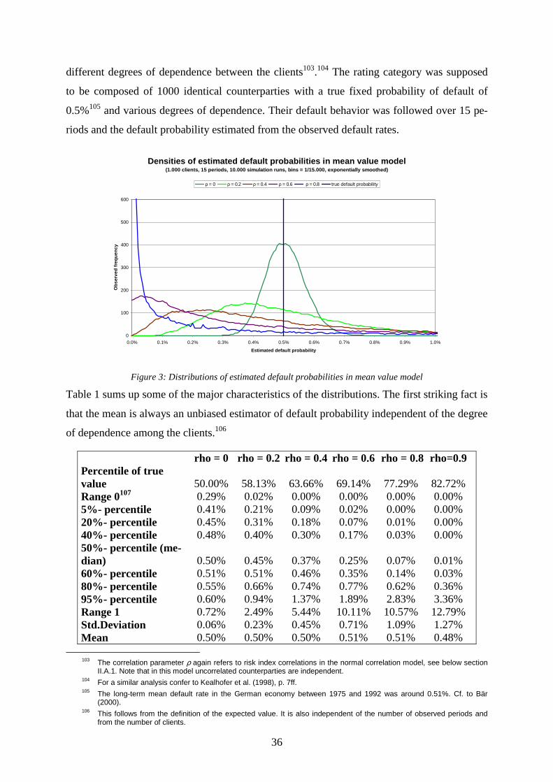
36

different degrees of dependence between the clients103.104 The rating category was supposed

to be composed of 1000 identical counterparties with a true fixed probability of default of

0.5%105 and various degrees of dependence. Their default behavior was followed over 15 pe-

riods and the default probability estimated from the observed default rates.

Densities of estimated default probabilities in mean value model(1.000 clients, 15 periods, 10.000 simulation runs, bins = 1/15.000, exponentially smoothed)

0

100

200

300

400

500

600

0.0% 0.1% 0.2% 0.3% 0.4% 0.5% 0.6% 0.7% 0.8% 0.9% 1.0%

Estimated default probability

Obs

erve

d fre

quen

cy

ρ = 0 ρ = 0.2 ρ = 0.4 ρ = 0.6 ρ = 0.8 true default probability

Figure 3: Distributions of estimated default probabilities in mean value model

Table 1 sums up some of the major characteristics of the distributions. The first striking fact is

that the mean is always an unbiased estimator of default probability independent of the degree

of dependence among the clients.106

rho = 0 rho = 0.2 rho = 0.4 rho = 0.6 rho = 0.8 rho=0.9Percentile of true value 50.00% 58.13% 63.66% 69.14% 77.29% 82.72% Range 0107 0.29% 0.02% 0.00% 0.00% 0.00% 0.00% 5%- percentile 0.41% 0.21% 0.09% 0.02% 0.00% 0.00% 20%- percentile 0.45% 0.31% 0.18% 0.07% 0.01% 0.00% 40%- percentile 0.48% 0.40% 0.30% 0.17% 0.03% 0.00% 50%- percentile (me-dian) 0.50% 0.45% 0.37% 0.25% 0.07% 0.01% 60%- percentile 0.51% 0.51% 0.46% 0.35% 0.14% 0.03% 80%- percentile 0.55% 0.66% 0.74% 0.77% 0.62% 0.36% 95%- percentile 0.60% 0.94% 1.37% 1.89% 2.83% 3.36% Range 1 0.72% 2.49% 5.44% 10.11% 10.57% 12.79% Std.Deviation 0.06% 0.23% 0.45% 0.71% 1.09% 1.27% Mean 0.50% 0.50% 0.50% 0.51% 0.51% 0.48%

103 The correlation parameter ρ again refers to risk index correlations in the normal correlation model, see below section

II.A.1. Note that in this model uncorrelated counterparties are independent. 104 For a similar analysis confer to Kealhofer et al. (1998), p. 7ff. 105 The long-term mean default rate in the German economy between 1975 and 1992 was around 0.51%. Cf. to Bär

(2000). 106 This follows from the definition of the expected value. It is also independent of the number of observed periods and

from the number of clients.

37

Skewness 2,10E-11 1,71E-08 2,22E-07 1,14E-06 4,63E-06 7,31E-06Kurtosis 3,47E-13 2,01E-10 5,31E-09 4,55E-08 2,62E-07 4,38E-07

Table 1: Characteristics of simulated distributions of probability estimator in the mean value model

Conversely, the distributions’ standard deviations, their skewness’, kurtosis’, and ranges, and

the percentile represented by the true default probability do increase with the degree of de-

pendence108.

The case of independent clients is set off against the case of higher correlations because here

the average default rate is normally distributed due to the central limit theorem. This is quite

well indicated by the simulation results since the normal distribution is symmetric around the

mean109 with zero skewness and kurtosis. The instance of independence is the only one where

the average default rate is already a consistent estimator of default probability when the num-

ber of clients tends to infinity110.

If correlations are positive, the standard deviation of the average default rate remains positive

even if the number of clients in this rating category is infinitely large, although it is decreas-

ing in the number of clients. If, however, the number of periods goes to infinity, the default

probability can be consistently estimated no matter how many clients there are.111

107 Range 0 is the 0%-centile, i.e. the smallest simulated value of the average default rate. Equivalently, range 1 is the

100%-centile, i.e. the highest simulated value. 108 An animation that illustrates the dependence of the distribution of the mean default rate on the number of periods of

data available and the correlations between clients is available at http://www.risk-and-evaluation.com/Animation/Mean_Value_Model.gif

109 This is why the mean and the median are identical. 110 This means that the average default rate converges stochastically against the true default probability in the number of

clients. Consistency implies that the precision of the estimation improves if the amount of available data increases, and that

the sampling error diminishes. 111 It is straightforward to show that the standard deviation σ of the average default rate can be directly calculated as

2/1

)1(1

1)1(11

),,,(

−−+−= pp

npp

nmpnm DD ρρσ

where m is the number of periods observed, n is the number of clients, p the true probability of default and ρD = ρD(ρ,p) is the default correlation. In the normal correlation model, ρD is given by

( ) ( ) ( )

( ) ( )( )aa

aaaa

Φ−Φ

ΦΦ−Φ=

1

;,D

ρρ

with Φ(⋅) being the one dimensional cumulative normal distribution function, Φ(⋅,⋅; ρ) the two dimensional cumulative normal distribution function with correlation ρ, and finally with a = Φ-1(p).

If the number of clients n goes to infinity, σ converges monotonously decreasingly to

2/1

)1(1

→ −∞→ ppm

n Dρσ

If, on the other hand, the number of periods m tends to infinity, σ apparently goes to zero. Thus, since the average de-fault rates at single periods are independent and identically distributed by assumption, the overall mean default rate converges stochastically to the true probability of default by the law of large numbers. Note that it would be sufficient that average default rates are uncorrelated and have the same mean. Serial independence is not necessary for con-sistency. Also may dependencies among clients change over time as long as default probabilities remain constant.

However, at least the assumption of serially uncorrelated observations is crucial in the mean value model since other-wise a consistent estimation of default probabilities would be impossible. Together with the hypothesis that default

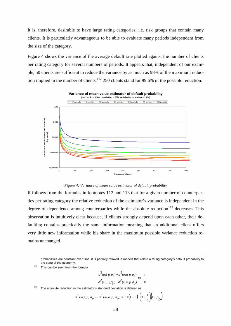
38

It is, therefore, desirable to have large rating categories, i.e. risk groups that contain many

clients. It is particularly advantageous to be able to evaluate many periods independent from

the size of the category.

Figure 4 shows the variance of the average default rate plotted against the number of clients

per rating category for several numbers of periods. It appears that, independent of our exam-

ple, 50 clients are sufficient to reduce the variance by as much as 98% of the maximum reduc-

tion implied in the number of clients.112 250 clients stand for 99.6% of the possible reduction.

Variance of mean value estimator of default probability(def. prob. = 0.5%, correlation = 20% ⇒ ⇒ ⇒ ⇒ default correlation = 1.6%)

0,000001

0,00001

0,0001

0,001

0,01

0 50 100 150 200 250 300 350 400

Number of clients

Varia

nce

of e

stim

ated

def

ault

prob

ilitie

s (lo

g sc

ale)

2 periods 5 periods 10 periods 15 periods 20 periods 25 periods 30 periods

Figure 4: Variance of mean value estimator of default probability

If follows from the formulas in footnotes 112 and 113 that for a given number of counterpar-

ties per rating category the relative reduction of the estimator’s variance is independent in the

degree of dependence among counterparties while the absolute reduction113 decreases. This

observation is intuitively clear because, if clients strongly depend upon each other, their de-

faulting contains practically the same information meaning that an additional client offers

very little new information while his share in the maximum possible variance reduction re-

mains unchanged.

probabilities are constant over time, it is partially relaxed in models that relate a rating category’s default probability to the state of the economy.

112 This can be seen from the formula

npmpm

pnmpm

DD

DD 11

),,,(2

),,1,(2

),,,(2

),,1,(2

−=∞−

−

ρσρσ

ρσρσ.

113 The absolute reduction in the estimator’s standard deviation is defined as

( ) ( )Dn

pppnmpm DD ρρσρσ −−⋅−⋅=−

1

111),,,(),,1,(

22 .

39

Analogously, 5 periods of data diminish the estimator’s variance by 80% of the maximum, 10

periods by 90% and 30 periods by 96.7%.114 Note again that the impact of the number of pe-

riods of available data on the variance is unaffected by the degree of dependence among coun-

terparties.

Table 1 also shows that for a given number of periods and clients in the analysis, the percen-

tile that is represented by the true value of the probability of default increases with the level of

dependence among counterparties.

In case of independence, the true value equals the median of the distribution of the estimator.

Hence, one would expect to have a 50% chance to overestimate or to underestimate the cor-

rect value. If dependencies are rather elevated, though, it is considerably more likely to under-

state the accurate value than to overestimate it. Thus, especially in case of high correlations it

is important to seek to diminish the estimator’s variability.

d) How many rating categories should a financial institution distinguish?

Estimation errors implied by rating systems result from two major sources, the conceptual

imprecision that rating categories are homogeneous and a sampling error from the actual es-

timation of default probabilities.

Although it is simplifying, the assumption of homogeneous categories is necessary in the

mean value model to consistently perform all subsequent estimations. In order to use rating

systems efficiently in this context, one is, therefore, forced to try to simultaneously keep both

errors small.

As we have seen from the discussion, the supposition that all counterparties within one rating

category are equal as far as default probabilities are concerned is less problematical the more

categories there are. With an increasing number of categories the mean default probability

converges to the individual default probability of each counterparty. From this point of view,

many rating categories are good.

On the other hand, we have seen that the sampling error from the estimation of default prob-

abilities resulting from the random nature of observed default frequencies decreases with the

114 The relative reduction of the standard deviation in the number of available periods of data for a given number of clients

in the portfolio is equal to

mDD

DD

pnpn

pnmpn 11

),,,(2

),,,1(2

),,,(2

),,,1(2

−=∞−

−

ρσρσ

ρσρσ .

40

number of clients per group. Hence, from this point of view, many clients per category are

good. This implies, however, that the total number of clients in the portfolio should not be

divided by too large a number of categories.

Both objectives are, thus, completely contradictory. Nevertheless, to optimize results a num-

ber of rules can be set up:

1. there should be at least 50-100 clients per rating category. If there are fewer clients, the

variance of the estimator of default probability increases drastically due to the small num-

ber. This requirement limits the number of categories.

2. use rating categories efficiently. An ‘investment’ grade should be defined for areas of high

exposure concentration. Distinguish more categories within the investment grade than in

the remaining speculative grade. This reduces the estimation error on the portfolio level.

3. if a bank is too small to provide the necessary number of clients, another bank could be

found with a similar structure so that they can pool their data to perform the estimations.

4. to facilitate a closer cooperation between financial institutions, it should be possible to

render the first step in the rating process, i.e. the evaluation of clients’ risk profiles and the

assignment of a risk score, transparent to other banks.

5. not controversial, but also crucial is an effective early warning system to be sure that ac-

tual rating assignments are up to date and exposures are correctly calculated.

6. finally, the rating process should be stable over time to allow the maximum number of

periods of default experience to be included in the analysis.

The number of rating categories that a financial institution should distinguish depends pre-

dominantly on its size and on the structure of its business. Large banks can use more catego-

ries than small banks. Institutions that hand out considerable amounts of money to all risk

grades need more categories than banks with a rather conservative profile.

5. Rating based estimation of default probabilities: Credit Risk +

An important assumption in the mean value model was that default probabilities of each rat-

ing grade are constant over time, only observed default frequencies vary from period to pe-

41

riod. A different approach was chosen in the Credit Risk + model developed by Credit Suisse

Financial Products115 between 1993 and 1996.

a) Main concept

In this model, default probabilities are themselves stochastic. Each period nature is thought to

independently draw a default probability from a probability distribution. Only as a second

step actual defaults occur depending on the sampled default probability. Because default be-

havior is found to differ significantly between industries, the law from which a default prob-

ability is drawn depends on rating category and sector.

The variation of default probabilities is explained by background factors upon which clients

systematically depend116. Their nature is not further specified and remains anonymous. All

necessary information concerning systematic influences on default behavior is assumed to be

contained in the probability law determining the development of default probabilities.

Note that although default probabilities are random in the model, the probability law that con-

trols them is presumed to be constant. It seems paradoxical, but it is essentially the concept of

continuity that is different in Credit Risk + from the mean value model.


There are two main driving forces behind the conceptual architecture of Credit Risk +: firstly,

the analytical derivation of the loss distribution for a portfolio of clients and, secondly, the

mathematical necessity when it comes to estimating the required inputs. Hence, technical rea-

sons have a very high priority in Credit Risk +.

The model supposes default probabilities to follow a gamma law117. The motive for this as-

sumption is the well known compatibility of the gamma distribution to the Poisson distribu-

tion that leads to the desired analytical result for the portfolio loss distribution. The Poisson

law is relevant in the second step of the modeling process. It describes the number of defaults

per period in an industry/rating segment in Credit Risk +118 once the probability of default is

fixed.

115 See Credit Suisse Financial Products (1996). Credit Risk + is mainly an adaptation of the compound Poisson model

frequently used in insurance mathematics. 116 See Credit Suisse Financial Products (1996), p. 20. 117 This choice might surprise at first sight because the gamma law takes values on the whole positive real axis with posi-

tive probability. The probability to draw a default probability that is greater than 1 is negligible in realistic situations, though.

118 For technical details confer to Credit Suisse Financial Products (1996), p. 32ff.

42

The supposition of the Poisson law as the distribution of the number of defaults for a known

probability of default is only justified if defaults are independent. Indeed, if default probabili-

ties are fixed and equal for all clients119, and if counterparties are independent, it can be

shown that the number of defaults in that period follows a Poisson distribution120. If, however,

counterparties are not independent, this implication would be wrong.

The assumption of independent defaults conditional to a given default probability is crucial in

Credit Risk + also for a further cause. The gamma law from which default probabilities are

drawn has two free parameters, both of which are functions of the expected value and the

standard deviation of default probability.121 The expected value can be consistently estimated

by the mean of default frequencies as long as they are serially uncorrelated no matter how

defaults depend upon each other at a certain point in time122. For the standard deviation

things are more difficult. It is a problem to derive an estimator for it if the degree and the ex-

act form of dependence between defaults are not fully specified. In case of independence,

however, all joint distributions of defaults are known.

c) Discussion

In Credit Risk+, the focus is not on the exact modeling and estimation of default probabilities.

The authors do not say much about the estimation of hidden input variables, especially of the

volatility of default probabilities123. This is so much more fundamental as this task is not

selfexplicatory despite the strict assumptions.

In his comparison of Credit Metrics and Credit Risk + Michael Gordy describes a way to es-

timate the standard deviation of default probabilities.124 The estimator is given as

119 This is again the assumption of homogeneity in a risk group that already occurred in the mean value model. Note that

in this context a risk group is defined as a combination of rating and sector. 120 The Poisson approximation of the binomial distribution is an asymptotic result for the number of clients going to infinity.

Hence, it would also be required that the number of clients in a segment is arbitrarily large. This turns out to be a prob-lem in the long run because in Credit Risk + segments are further subdivided by exposure size in order to be able to calculate their loss distributions merely from knowing the distribution of the number of defaults in the segment. In con-sequence, the loss distribution resulting from the portfolio analysis in Credit Risk + can, firstly, take values with positive probability that are larger than the portfolio value and, secondly, the loss distribution is less discontinuous than it would be implied by real exposures because the jumps are filled up with imaginated defaults of small exposures. For further discussion see below section II.A.3.a).

For the estimation of default probabilities and volatilities, exposure size in not relevant, however, so that this problem can be neglected here.

121 See Credit Suisse Financial Products (1996), p. 45. 122 This follows from the law of large numbers. 123 See Credit Suisse Financial Products (1996), p. 12f. Apparently, the authors suppose that practitioners would use re-

sults published by rating agencies. For not publicly rated companies or private customers this might be doubtful. 124 Gordy (2000), p.24.

43

( ) ( ) ( )η

η−

−−=1

1ˆˆˆ pppVpV ,

where )(ˆ pV stands for the estimated variance of p, p for default probability, ( )pV ˆˆ for the es-

timated variance of the observed default frequency in period t, p for the average observed

default frequency, and η for the average number of counterparties in the industry / rating

segment125.

Note that this variance estimator leads to invalid results if

( ) ( )pppV −< 1ˆˆ η

where the estimated variance takes on negative values. Simulation results show that this hap-

pens more frequently the smaller default frequencies and true default volatilities are and the

fewer periods are available for evaluation.126

Simulated frequencies of invalid volatility estimations in Credit Risk +

(10.000 Simulation runs, volatility of default prob. = mean default prob. = dp)

0%

5%

10%

15%

20%

25%

30%

35%

0 100 200 300 400 500 600 700 800 900 1000

Number of counterparties

Sim

ulat

ed fr

eque

ncy

0.5% dp / 10 periods 1% dp / 10 periods 1.5% dp / 10 periods0.5% dp / 15 periods 1% dp / 15 periods 1.5% dp / 15 periods

Figure 5: Frequency of invalid volatility estimations in Credit Risk +

125 Let in be the number of firms in the industry / rating-segment in period i = 1,…, m. Then η is given as

∑==

m

i inm

1

11η

126 Default probabilities were simulated from the gamma law with default volatilities being equal to default probabilities. In this case the density function of the gamma distribution has the simple form

σ

σ

x

exf−

=1

)(

with σ being the volatility of default probabilities. Random variates can be easily generated by inversion of the cumula-tive distribution function. Having drawn a default probability for one period, independent defaults were simulated for the respective number of counterparties. This was repeated for the required number of periods and the results served as input for the estimation of default volatility. The whole procedure was repeated 10.000 times to generate the distri-bution of the estimator.

44

It also turned out that the volatility estimator in Credit Risk + is consistent, but biased in small

samples. The volatility is expected to be largely understated if the number of clients and the

number of periods are small. Having 5 or more periods of data, the estimation error caused by

a small number of clients seems to be minimized if there are at least 200 clients in the indus-

try / rating segment. Due to the decomposition of the portfolio by two criteria, rating and in-

dustry, this implies a financial institution that distinguishes 10 rating grades and has custom-

ers in 15 sectors to have at least 30.000 clients evenly distributed over the risk groups. This is

a harsh requirement since there are always some segments that are only sparsely populated. In

these risk groups a significant estimation error is to be expected.

Expected values of the volatility estimator in Credit Risk +- dependence on number of periods and number of clients -(Mean default probability = 0.5% = true volatility of default prob., 1.000 simulation runs)

-80%

-60%

-40%

-20%

0%

20%

40%

60%

0 50 100 150 200 250 300 350 400 450 500

Number of clients

Rel

ativ

e bi

as o

f exp

ecte

d va

lue

2 periods 5 periods 10 periods 15 periods 20 periods 25 periods 30 periods

Figure 6: Bias of estimated default rate volatility in Credit Risk + dependent on number of periods and number of clients

It is remarkable that for 30 to 50 clients in a segment the default rate volatility is overstated if

there are many periods of data. This is because the components of the estimator that increase

or decrease, resp., in the number of periods and / or clients superimpose so that the estimated

volatility of default reaches a peak if the segment is middle-sized and if the time series is

long.

Figure 7 illustrates that the bias in the estimation of default volatility caused by a small num-

ber of periods of data is slow to disappear. Having observations over 15 periods, the volatility

is still expected to be systematically understated by as much as 5%. Taking into consideration

that default volatility is one of the main risk drivers in Credit Risk +, this result is quite wor-

rying because only very few banks have this long history of observations.

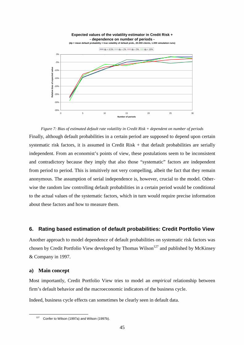
45

Expected values of the volatility estimator in Credit Risk +- dependence on number of periods -

(dp = mean default probability = true volatility of default prob., 20.000 clients, 1.000 simulation runs)

-35%

-30%

-25%

-20%

-15%

-10%

-5%

0%

0 5 10 15 20 25 30

Number of periods

Rel

ativ

e bi

as o

f exp

ecte

d va

lue

dp = 0.5% dp = 2% dp = 5% dp = 10%

Figure 7: Bias of estimated default rate volatility in Credit Risk + dependent on number of periods

Finally, although default probabilities in a certain period are supposed to depend upon certain

systematic risk factors, it is assumed in Credit Risk + that default probabilities are serially

independent. From an economist’s points of view, these postulations seem to be inconsistent

and contradictory because they imply that also those “systematic” factors are independent

from period to period. This is intuitively not very compelling, albeit the fact that they remain

anonymous. The assumption of serial independence is, however, crucial to the model. Other-

wise the random law controlling default probabilities in a certain period would be conditional

to the actual values of the systematic factors, which in turn would require precise information

about these factors and how to measure them.

6. Rating based estimation of default probabilities: Credit Portfolio View

Another approach to model dependence of default probabilities on systematic risk factors was

chosen by Credit Portfolio View developed by Thomas Wilson127 and published by McKinsey

& Company in 1997.

a) Main concept

Most importantly, Credit Portfolio View tries to model an empirical relationship between

firm’s default behavior and the macroeconomic indicators of the business cycle.

Indeed, business cycle effects can sometimes be clearly seen in default data.

127 Confer to Wilson (1997a) and Wilson (1997b).

46

Observed and estimated default frequencies in the German economy 1976-1992

(Source: Statistisches Bundesamt der Bundesrepublik Deutschland, own calculations)

0.0%

0.1%

0.2%

0.3%

0.4%

0.5%

0.6%

0.7%

0.8%

0.9%

1976 1978 1980 1982 1984 1986 1988 1990 1992

Year

Def

ault

freq

uenc

y

observed default frequencies Estimated default frequencies using an AR(1)-model Mean default frequency

Figure 8: Observed and estimated default frequencies in the German economy 1976-1992

Figure 8 shows annual default rates for the entire German economy from 1976 to 1992128.

From 1976 to 1981 default rates are well below average, from 1981 to 1988 they are consid-

erably higher than average and in the period from 1988 to 1992 they sink once again. There-

fore, using the mean value model, default rates are systematically overestimated in good peri-

ods and also heavily understated during recessions. The idea to relate observed default fre-

quencies to macroeconomic data is, thus, well founded in the data.

However, two important adaptations have to be made. Producing different kinds of goods and

services, all industries are not equally integrated into the macroeconomy. Wilson shows that

there are major differences in annual fluctuations of default rates across industries finding

that, for instance, construction is strongly and energy and mining are hardly affected by the

business cycle129. The analysis of companies default behavior should, therefore, take account

of their industry.130

It is also a well known fact that business cycle effects strongly depend upon a firm’s general

financial condition. Firms with a weak market position are hit much harder by a recession

than highly competitive companies. Indeed, a default of an actual AAA-company has never

been observed no matter what the macroeconomic environment was. What is more, the mac-

roeconomic dependence of investment grade companies is hardly detectable. Hence, Wilson

chooses to use an industry’s speculative grade companies as an indicator of that industry’s

128 The data comprises all VAT payers in Germany, i.e. altogether around 4 mio. firms of all sizes, ratings, and industries.

For details confer to Bär (2000), p. 2. 129 Wilson (1997a), p.112f. 130 Wilson does not discuss the case of companies that operate in several industries.

47

economic health. In a further step he then indirectly derives default and migration probabili-

ties of specific rating grades in that industry.

However, Credit Portfolio View goes further. The aim is not only to explain firms’ actual de-

fault behavior, but also to forecast their default probabilities over the whole life of the longest

lasting contract in the bank’s portfolio, this is well over 10-30 years in the future131. It is ar-

gued that some contracts are highly illiquid so that a bank is forced to hold them to maturity,

even if the credit quality of the counterparty deteriorates. In order to capture this kind of con-

tract’s credit risk appropriately, the client’s default probability has to be adapted to its time

horizon.


In order to achieve this, Credit Portfolio View proceeds in three steps132:

1. It begins with a model of the future development of the relevant macroeconomic fac-

tors133. The model is fitted using historical macroeconomic data. By drawing prediction

errors randomly, the macroeconomic development is simulated over the desired time hori-

zon.

2. Secondly, a multi-factor model is chosen to describe the relationship between annual de-

fault rates of speculative grade companies in each industry and macro factors. Again, the

model is fitted using historical data, and future annual default probabilities of speculative

grade companies are simulated by random choice of prediction errors.

3. Finally, the simulation results are used to calculate conditional default and migration

probabilities for each year and rating grade up to the end of the time horizon.

For each country / industry combination three macroeconomic factors are chosen und mod-

eled by univariate autoregressive processes such as AR(p) or ARIMA(p,d,q). All parameters

are estimated with least squares techniques. The vector εmacro,t of estimation errors of the fitted

factor models is assumed to be normally distributed with mean 0 and covariance matrix Σmacro.

Σmacro has to be estimated from historical data. To extend the factors’ historical time series

into the future, error terms εmacro,t are simulated by independent draws from the specified dis-

tribution using standard techniques.

131 Wilson (1997a), p. 113. 132 Wilson (1997a), p. 114 133 This model may include global factors, but it is designed to explain the country (and industry) specific default behavior.

48

To make sure that all simulated future default probabilities take values between 0 and 1, ob-

served speculative default rates are mapped to the whole real axis by the logit transformation

( )

−==

it

ititit p

ppLy

,

,,,

1ln

where pt,i is the observed default rate in period t and sector i and yt,i is the transformed default

rate134. yt,i is then linearly regressed against the explaining macroeconomic variables X1,i,t,…,

Xn,i,t relevant for sector i

tideftinintiiioit XXy ,,,,,,,1,1,, εβββ ++++=

where β0,i, ..., βn,i are unknown parameters. Again, the parameters are estimated with least

squares techniques applied to the transformed default rates135, and error terms are assumed to

be normally distributed with mean 0 and covariance matrix Σdef. Future values of yt,i are simu-

lated by drawing independent error terms from this distribution136 and then retransformed into

default probabilities by the inverse logit function

( ))exp(1

1

,,

1,

ititit y

yLp+

== − .

The last step, the derivation of conditional transition matrices is not well documented in Wil-

son’s publications. It is merely indicated that the ratio of the simulated speculative default

probability pt,i for the future period t to the mean default probability ip , thus,

i

it

pp , ,

serves as an indicator as to what extent transition probabilities might have changed compared

to the long term mean due to the simulated macroeconomic background, from which a condi-

tional annual migration matrix

i

ij

pp

M , is obtained. A Markov assumption137 then yields a t-

year cumulative transition matrix

134 Note that, as in Credit Risk +, defaults are supposed to be independent conditional to a macroeconomic scenario. 135 Cf. to Bär (2000), p. 2 and 12. This estimation technique is also used in McKinsey’s software implementation of Credit

Portfolio View, cf. McKinsey (1999), p. 36. 136 Precisely, Wilson allows for covariances between εmacro and εdef and simulates all errors simultaneously. 137 The Markov assumption means that a firm’s transition probability in period t merely depends upon its actual rating at

the beginning of period t and not on its full migration path in the past.

49

∏=

=

t

j i

ijit p

pMM

1

,, .

c) Discussion

The intention to relate firms’ historic default frequencies to observable systematic risk factors

such as macroeconomic indicators is clearly the main advantage of Credit Portfolio View in

comparison to Credit Risk + or the mean value model.

For a number of reasons, it is, however, doubtful whether this goal really has been achieved.

(1) Modeling of macroeconomic processes

Credit Portfolio View describes the underlying macroeconomic factors by autoregressive

processes, i.e. by processes whose future development is exclusively explained by their own

history.138 Aiming at a long-term prediction of factors and default behavior, this feature is

clearly advantageous with regard to a software implementation for it renders the necessary

simulations extremely easy to carry out as it does not require any further input. For two rea-

sons, autoregressive processes are problematical choices as models for macro factors.

Firstly, from an economist’s standpoint, it is uncertain whether the macroeconomic factors

given as examples by Wilson139 such as the unemployment rate, GDP growth rate, rate of

government spending etc. can well be described relying only upon their own past. Even more

than equity market data these factors strongly depend on factors such as the results of elec-

tions, on political decisions, and the will to carry out reforms. All of those events are contin-

gent in nature and unrelated to the past. This is why it is so difficult to forecast them.

Secondly, the persistence of shocks and extreme values is relatively large in autoregressive

processes. If they are used as a model for macroeconomic factors in a credit risk model, the

effect of an economic crisis will be felt for many years.

Figure 9 compares the conditional mean default probability of speculative grade companies t

years after a crisis with their unconditional mean default probability. In both cases it is as-

sumed that reality functions exactly as Credit Portfolio View supposes and that all parameter

values are known and do not have to be estimated140. It is clearly visible that 30 years after the

138 And white noise. 139 Wilson (1997a), p. 113. 140 The macroeconomic factor is described by the AR(2)-process

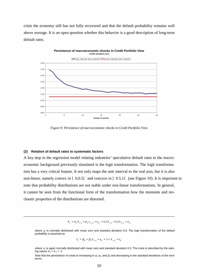
50

crisis the economy still has not fully recovered and that the default probability remains well

above average. It is an open question whether this behavior is a good description of long-term

default rates.

Persistence of macroeconomic shocks in Credit Portfolio View10,000 simulation runs

0.8%

0.9%

1.0%

1.1%

1.2%

1.3%

1.4%

1.5%

1.6%

0 5 10 15 20 25 30

Number of periods

cond. mean def. prob. in period t uncond. mean def. prob. in period t

Figure 9: Persistence of macroeconomic shocks in Credit Portfolio View

(2) Relation of default rates to systematic factors

A key step in the regression model relating industries’ speculative default rates to the macro-

economic background previously simulated is the logit transformation. The logit transforma-

tion has a very critical feature. It not only maps the unit interval to the real axis, but it is also

non-linear, namely convex in [0,0.5] and concave in [0.5,1] (see Figure 10). It is important to

note that probability distributions are not stable under non-linear transformations. In general,

it cannot be seen from the functional form of the transformation how the moments and sto-

chastic properties of the distributions are distorted.

XttXtXtt XXXX εεαα ++=++= −−−− 212211 2.02.0

where εX is normally distributed with mean zero and standard deviation 0.9. The logit transformation of the default probability is assumed as

YtYtt XXY εεββ ++=++= −− 1110 5

where εY is again normally distributed with mean zero and standard deviation 0.3. The crisis is described by the start-ing values X0 = X-1 = -1.

Note that the persistence of crises is increasing in α1,α2, and β1 and decreasing in the standard deviations of the error terms.

51

Logit transform

-6

-4

-2

0

2

4

6

0 0.1 0.2 0.3 0.4 0.5 0.6 0.7 0.8 0.9 1

Inverse logit transform

0

0.1

0.2

0.3

0.4

0.5

0.6

0.7

0.8

0.9

1

-5 -4 -3 -2 -1 0 1 2 3 4 5

Figure 10: Logit and inverse logit transformation

Realistic default probabilities can be assumed to be smaller than 50% even in bad times, thus,

the logit transformation is convex in the relevant area. To see the effect of a convex transform

on a distribution, assume an arbitrary random variable X with expectation µ. Let g(x) be a

convex transform defined in the domain of variation of X. Then there exists a line through the

point (µ,g(µ)) that lies fully below the graph of g (see Figure 11).

Convex transforms and probability distributions

x

y

Figure 11: Convex transforms and probability distributions

Thus,

)()()( µµ −+≥ xcgxg

for all x. If Y = g(X) has finite expectation, it follows from the monotonicity and linearity of

the Lebesgue-integral that141

141 This result is known as Jensen’s inequality.

µ

g(µ)

y=g(µ)+c(x-µ)

y = g(x)

(µ,g(µ))

52

( ) [ ]

)()()()()(

)()()()()()(

01

µµµ

µµ

gxdFxcxdFg

xdFxcgxdFxgxgE

=−+=

−+≥=

=

∞

∞−

=

∞

∞−

∞

∞−

∞

∞−

∫∫

∫∫

Hence, we have

( ) )()( µgxgE ≥ .

Note that there is equality only for deterministic random variables, i.e. if P(X=µ) = 1.

This implies for Credit Portfolio View that the expectations of each period’s transformed de-

fault rates conditional to the actual macroeconomic setting are greater than the transformed

default probabilities. This happens unless the exact conditional default probabilities are ob-

served each period with probability one. Although conditional independence had been as-

sumed142, it follows from the law of large numbers and the central limit theorem that this is

only the case if there are infinitely many speculative grade companies in each industry in the

financial institutions portfolio.

If there is only a finite number of speculative grade companies in each industry, default rates

cannot be understood as default probabilities. The regression against the macroeconomic fac-

tors is then performed with expectations of too high transformation results of observed default

rates. Since a linear regression is unbiased by construction, the estimated regression line will

be above the true regression line, even if the model is correctly specified143. Hence, the values

that are simulated according to the estimated regression line are too, in turn, too high.

Finally note that the inverse logit transformation decreases strictly monotonously. If the simu-

lated values are too high then the retransformed values, i.e. the simulated default probabilities,

are too low due to the decreasing retransformation.

Thus, if there are only a finite number of speculative grade companies in each industry, esti-

mation results, and in consequence simulation results, are biased towards too low probabilities

of default. The default risk is systematically underestimated in Credit Portfolio View.

142 If the model is not exact in that respect that macroeconomic factors don’t fully explain dependencies between clients,

the assumption that one period’s default rates are a consistent estimator of that period’s default probability is generally invalid. Confer to the discussion in footnote 111.

143 I.e. the error occurs even if reality functions exactly as the model supposes.

53

(3) Example

To illustrate this effect, we suppose that the true relationship between the macroeconomy and

firms’ default behavior is exactly as described in Credit Portfolio View. This means, we do

not take account of what was said at the beginning of the discussion and assume that there is

no general modeling error.

We consider an industry whose default behavior depends only on one macroeconomic factor.

Let’s presume that this factor X follows an AR(2)-process, precisely let

Xttt XXX ε1.04.04.0 21 ++= −−

where Xε is i.i.d. standard normally distributed. In order to isolate the systematic estimation

error in the next step, we assume that the parameters of the macroeconomic process are

known so that no further error at this point occurs.

The true regression model that relates transformed default probabilities to the macroeconomic

factor is set as

Ytt XY ε++= −15 .

The error term εY is supposed to be i.i.d. normally distributed with mean zero and known

standard deviation σ = 0.3. Note that only the last period’s realization of the systematic factor

is needed to estimate or predict the present period’s transformed default probability. Again we

assume that the general form of the regression model in known. Only the two parameters β0 =

5 and β1 = 1 are to be estimated.

While the long-term mean probability of default depends on both parameters, β0 certainly has

the dominant influence. Since the inverse logit transformation decreases monotonously, high

values of β0 correspond to low default probabilities.144

In order to fit the model, a historical time series of n periods of unknown default probabilities

and observed default frequencies for various numbers of counterparties in the industry was

simulated upon which the estimations could be based. Having performed the estimations, de-

fault probabilities were simulated for the next n periods. The additional problem of a predic-

tion horizon much longer than the history of observations was avoided.

144 The long-term mean probability of default is increasing in β1.

54

Bias of estimated long-term mean default probability in Credit Portfolio View

(true mean = 0.707%, 5,000 simulation runs, exponentially smoothed)

0.0%

0.1%

0.2%

0.3%

0.4%

0.5%

0.6%

0.7%

0.8%

0 500 1,000 1,500 2,000 2,500 3,000

Number of clients

Estim

ated

mea

n de

faul

t pro

babi

lity

20 periods 25 periods 30 periods true value

Figure 12: Bias of long-term mean default probability in Credit Portfolio View

Estimation error of estimated long-term mean default probability in Credit Portfolio View

(true mean = 0.707%, 5,000 simulation runs, exponentially smoothed)

-100%

-80%

-60%

-40%

-20%

0%

20%

0 500 1,000 1,500 2,000 2,500 3,000

Number of clients

Rela

tive

estim

atio

n er

ror

20 periods 25 periods 30 periods true value

Figure 13: Relative error of estimated long-term mean default probability in Credit Portfolio View

Figure 12 and Figure 13 clearly show that the long-term mean probability of default of the

process is consistently understated, even if there are up to 3,000 speculative145 grade firms in

a particular industry in the bank’s portfolio. This amount is certainly very rare. Especially the

relative estimation error is considerable since the quantity to be estimated is so small.

The picture is even more transparent if we look at the parameter estimates146.

145 Moody’s Investors Service and Standard and Poor’s define a speculative grade company as having a lower rating

grade than Baa or BBB, respectively. This corresponds to a default probability of more than 0.2-0.3%. 146 Note that the bias of parameter estimates does not depend on the length of the prediction period.

55

Bias of estimated regression parameter ββββ0 in Credit Portfolio View 5,000 simulation runs

4

5

6

7

8

9

10

11

12

13

0 200 400 600 800 1,000 1,200 1,400 1,600 1,800 2,000

Number of clients

Mea

n pa

ram

eter

est

imat

e

5 periods 10 periods 15 periods 20 periods 25 periods 30 periods true value

Figure 14: Bias of estimated regression parameter β0 in Credit Portfolio View

As it should be, the expected value of the estimate of 0β does not depend on the length of the

time series of historical observations. This comes from the fact that the AR(2)-process de-

scribing the development of the systematic risk factor is stationary and, therefore, the true

default probabilities and the observed default frequencies are too. Since the estimation of the

regression parameters of the transformed default rates is unbiased the deviation of the ex-

pected value of the parameter estimate of the true parameter value, i.e. the bias, is merely

owed to the non-linearity of the logit transformation. As already mentioned, large values of

0β correspond to low default probabilities.

Albeit the mean of the parameter estimate does not depend upon the number of periods of

data available for analysis, its standard deviation does.

56

Standard deviation of estimated regression parameter ββββ0 in Credit Portfolio View

5,000 simulation runs

0

1

2

3

4

5

6

0 500 1,000 1,500 2,000 2,500 3,000 3,500 4,000 4,500 5,000

Number of clients

5 periods 10 periods 15 periods 20 periods 25 periods 30 periods

Figure 15: Standard deviation of estimated regression parameter 0β in Credit Portfolio View

Having few periods of data and few clients the variation of the estimate is remarkable. With

more than 3,000 clients in the segment, however, its variability almost exclusively depends on

the number of periods in the sample.

If the number of clients is very small, the probability of not observing a default at all is rela-

tively high even if each individual company’s default probability is quite high147. This is why

the volatility of the estimate declines again for a small number of counterparties.

The result is similar if we look at β1.

Bias of estimated regression parameter ββββ1111 in Credit Portfolio View 5,000 simulation runs

0

0.5

1

1.5

2

2.5

3

3.5

4

0 500 1,000 1,500 2,000 2,500 3,000

Number of clients

Mea

n pa

ram

eter

est

imat

e

5 periods 10 periods 15 periods 20 periods 25 periods 30 periods true value

Figure 16: Bias of estimated regression parameter β1 in Credit Portfolio View

147 If there are 50 independent counterparties, each defaulting with 2% probability, the likelihood of observing no default is

36.4%.

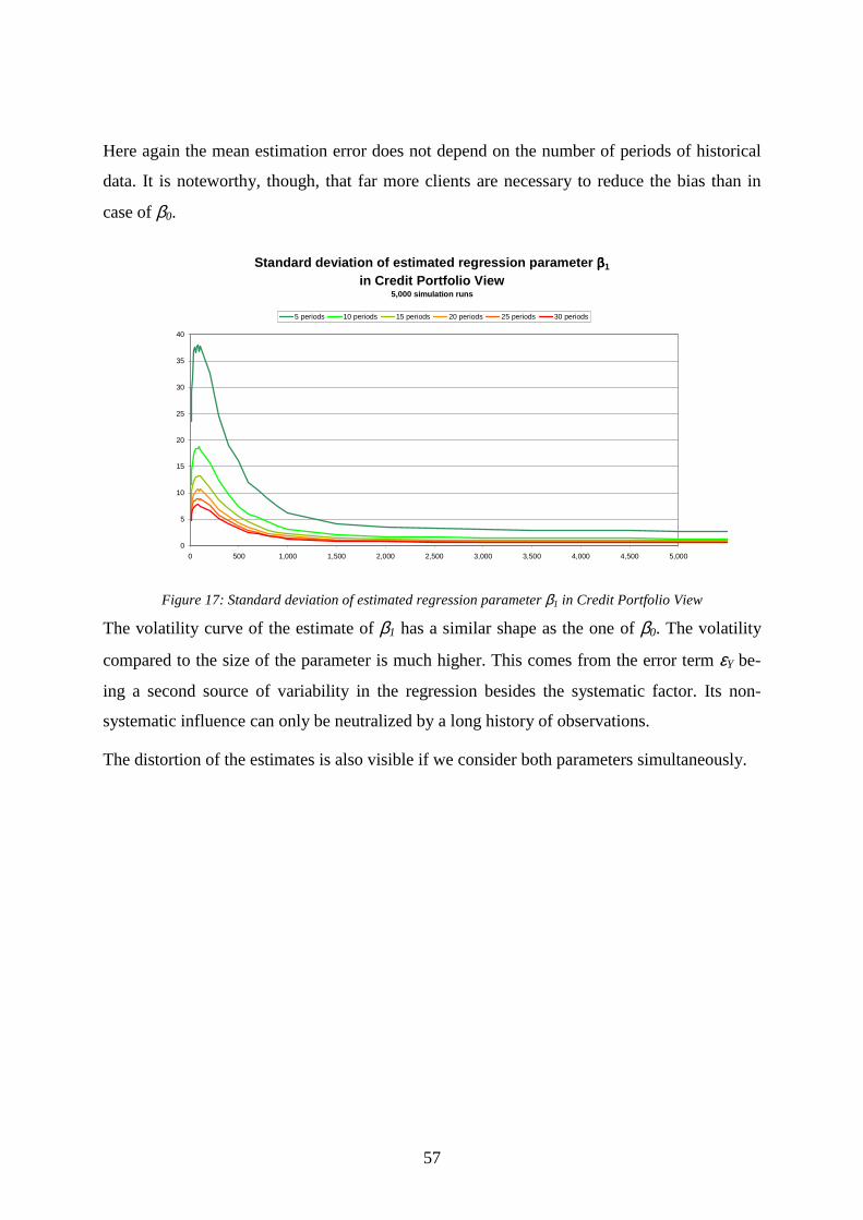
57

Here again the mean estimation error does not depend on the number of periods of historical

data. It is noteworthy, though, that far more clients are necessary to reduce the bias than in

case of β0.

Standard deviation of estimated regression parameter ββββ1 in Credit Portfolio View


0

5

10

15

20

25

30

35

40

0 500 1,000 1,500 2,000 2,500 3,000 3,500 4,000 4,500 5,000

5 periods 10 periods 15 periods 20 periods 25 periods 30 periods

Figure 17: Standard deviation of estimated regression parameter β1 in Credit Portfolio View

The volatility curve of the estimate of β1 has a similar shape as the one of β0. The volatility

compared to the size of the parameter is much higher. This comes from the error term εY be-

ing a second source of variability in the regression besides the systematic factor. Its non-

systematic influence can only be neutralized by a long history of observations.

The distortion of the estimates is also visible if we consider both parameters simultaneously.

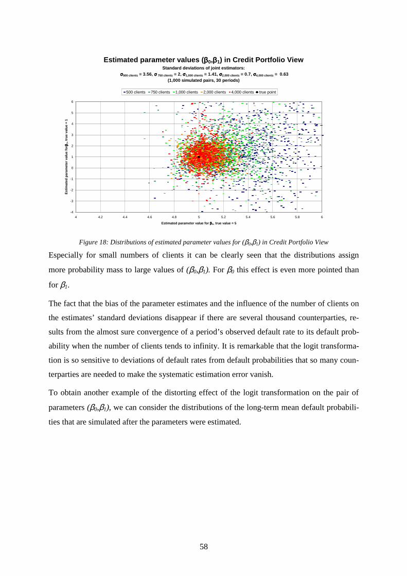
58

Estimated parameter values (ββββ0,ββββ1) in Credit Portfolio ViewStandard deviations of joint estimators:

σσσσ500 clients = 3.56, σσσσ 750 clients = 2, σσσσ1,000 clients = 1.41, σσσσ2,000 clients = 0.7, σσσσ4,000 clients = 0.63 (1,000 simulated pairs, 30 periods)

-4

-3

-2

-1

0

1

2

3

4

5

6

4 4.2 4.4 4.6 4.8 5 5.2 5.4 5.6 5.8 6

Estimated parameter value for ββββ0, true value = 5

Estim

ated

par

amet

er v

alue

for ββ ββ

1, tr

ue v

alue

= 1

500 clients 750 clients 1,000 clients 2,000 clients 4,000 clients true point

Figure 18: Distributions of estimated parameter values for (β0,β1) in Credit Portfolio View

Especially for small numbers of clients it can be clearly seen that the distributions assign

more probability mass to large values of (β0,β1). For β0 this effect is even more pointed than

for β1.

The fact that the bias of the parameter estimates and the influence of the number of clients on

the estimates’ standard deviations disappear if there are several thousand counterparties, re-

sults from the almost sure convergence of a period’s observed default rate to its default prob-

ability when the number of clients tends to infinity. It is remarkable that the logit transforma-

tion is so sensitive to deviations of default rates from default probabilities that so many coun-

terparties are needed to make the systematic estimation error vanish.

To obtain another example of the distorting effect of the logit transformation on the pair of

parameters (β0,β1), we can consider the distributions of the long-term mean default probabili-

ties that are simulated after the parameters were estimated.

59

Distributions of mean probabilities of default of estimated processes in Credit Portfolio View

(2,000 simulation runs, 30 periods, exponentially smoothed, true mean probability of default = 0.707%, bins = 0.01%)

0

20

40

60

80

100

120

140

160

0,0% 0,2% 0,4% 0,6% 0,8% 1,0% 1,2% 1,4%

Mean probability of default of estimated process

Freq

uenc

y500 clients 750 clients 1,000 clients 2,000 clients 4,000 clients true process true mean

Figure 19: Distributions of long-term mean probabilities of default of estimated processes in Credit Portfolio View

The plots displayed in Figure 19 were produced as follows. The true process was constructed

as in the example above. Parameters (β0,β1) were estimated based on a 30-year history of ob-

served data using a sample of 500 to 4,000 speculative grade companies in the industry under

consideration. Then default probabilities were simulated over the next 30 years and their

mean was calculated. This procedure was repeated 2,000 times to yield the distributions of the

long-term mean default probabilities.

500 clients 750 clients 1,000 clients 2,000 clients 4,000 clients true distribu-

tion Expectation 0,58% 0,64% 0,65% 0,69% 0,70% 0,71% Standard deviation 1,07E-02 4,29E-03 1,69E-03 1,10E-03 9,97E-04 6,83E-04 Skewness 3,89E-05 1,95E-06 2,44E-08 5,31E-10 3,98E-10 1,19E-10 Kurtosis 1,57E-05 2,94E-07 8,09E-10 9,80E-12 5,21E-12 6,69E-13 Range 0 0,07% 0,07% 0,18% 0,37% 0,40% 0,53% 5%- percentile 0,20% 0,34% 0,43% 0,53% 0,55% 0,60% 20%- percentile 0,33% 0,48% 0,55% 0,60% 0,62% 0,65% 40%- percentile 0,44% 0,57% 0,62% 0,65% 0,67% 0,69% 50%- percentile 0,50% 0,61% 0,65% 0,68% 0,69% 0,70% 60%- percentile 0,56% 0,65% 0,67% 0,70% 0,71% 0,72% 80%- percentile 0,70% 0,74% 0,75% 0,76% 0,77% 0,76% 95%- percentile 0,98% 0,90% 0,86% 0,87% 0,87% 0,83% Range 1 42,66% 16,23% 4,15% 1,45% 1,31% 0,97%

Table 2: Characteristics of distribution of long-term mean default rates in Credit Portfolio View

The characteristics of the distributions are summed up in Table 2. Three things become ap-

parent. Firstly, the expectation of the long-term mean default probabilities of the estimated

processes is systematically understated. Secondly, the same observation holds true for the

median of the distribution. The median of the true distribution corresponds to the 60%-

60

percentile if there are 4,000 clients in the sample up to the 80%-percentile if there are only

500. Thirdly, the bias decreases and standard deviation, skewness, kurtosis and span of the

simulated distribution converge to the respective characteristics of the true distribution as the

number of clients increases148.

It’s finally worth noting that the systematic estimation error in the regression of default rates

against macroeconomic factors in Credit Portfolio View is not due to the precise functional

form of the logit transformation, but rather to its non-linearity in combination with the estima-

tion techniques used. Any other non-linear transformation would cause a similar effect.

Hence, it would not help very much to replace the logit transformation by a probit transforma-

tion, for instance by the normal cumulative distribution function (cdf) which also only takes

values in the unit interval149. Other than the logit function, the inverse normal cdf is concave

in (0,0.5], so that the mean of the transformed default rates is smaller than their transformed

mean150. The normal cdf itself, that retransforms the regression results, monotonously in-

creases, so that the total estimation result understates the true values of default probabilities

once again.

(4) Conditional transition matrices

Even if default probabilities were correctly predicted, this is not the final step. The estimation

of default probabilities was not done for a specific rating grade, but for all ‘speculative grade’

companies together, i.e. for companies that are known to have different default and transition

probabilities. Thus, individual rating grades need to be adapted to macroeconomic scenarios.

For this purpose Wilson proposes another transformation of the estimated default probabilities

of the speculative grade firms in the respective industry depending on the ratio of the simu-

lated conditional default probabilitiy for a certain period and the estimated long-term mean

default rate.

Having seen that transformations can have a significant impact on the properties of a distribu-

tion and the precision of a model, it is particularly critical that the derivation of conditional

transition matrices is a gap in the documentation of Credit Portfolio View.

148 Note that standard deviation, kurtosis and span are necessarily larger at the estimated distributions because of the

unsystematic estimation uncertainty due to the finite number of periods in the sample that adds variability to the esti-mated distributions.

149 This is proposed in a context not related to Credit Portfolio View by Kim (1999). He suggests the normal cdf as a trans-form of default rates not to avoid estimation errors, but because Credit Metrics uses it to model rating migrations.

150 This is Jensen’s inequality again.

61

Apart from another possible systematic estimation error, this transformation is the third suc-

cessive estimation between macroeconomic risk factors and each specific rating grade’s mi-

gration probability, especially its default probability, where each step increases the variability

of the results. Let’s take an

(5) Example

The future macroeconomic situation becomes more and more independent of the present one

as the prediction horizon increases. Therefore, the simulated long-term mean cumulative

probabilities of default of each rating grade should converge to the historically observed long-

term averages. Using the Markov assumption mentioned above, n-year cumulative default

probabilities can easily be derived from the annual transition matrices published by the rating

agencies by multiplying the respective matrix n times with itself.151 If we compare the out-

come for a 10-year time horizon with the example given by Wilson152 for the German econ-

omy, we see that the results differ greatly.

Rating153 Extrapolation of Moody’s transition ma-

trix154

Wilson’s results

Ratio

AAA 0,47% 1,74% 374% AA 1,35% 4,12% 305% A 3,72% 9,58% 257%

BBB 9,71% 22,63% 233% BB 24,78% 46,75% 189% B 44,96% 69,12% 154%

CCC 68,55% 83,58% 122% Table 3: 10-year cumulative default probabilities extrapolated using Markov assumptions

The deviation is so much more striking as Wilson himself uses a Markov assumption and

Moody’s annual mean transition matrix155 to derive long-term transition matrices. Especially

for investment grade companies, the probabilities derived from Moody’s data only make up

less than half of Wilson’s findings. The transformation of speculative grade default probabili-

ties in rating specific ones is apparently no straightforward exercise. It does not seem

convincing to explain the results by a disastrous economic situation in Germany in 1997.

151 Wilson himself quotes Moody’s transition matrix, Wilson (1997a), p. 113, table A. We used this data for the extrapola-tion in Table 3. Note that Wilson quotes exactly the same matrix as Standard and Poor’s transition matrix in Wilson 1997c, figure 6.

152 Wilson (1997a), p. 117, table B. 153 It is Wilson’s terminology to use Standard and Poor’s notation for Moody’s rating grades (see also footnote 151). 154 See also footnote 151!. 155 It is actually not quite clear from Wilson’s article which rating agencies transition matrix he uses for his example. Note,

however, that Moody’s, Standard and Poor’s, and Fitch’s results are by and large similar.

62

The Markov assumption certainly facilitates the description of firms’ long-term default

behavior considerably. It is, however, not clear how close it is to reality. The Markov assump-

tion implies that there are no systematic consecutive downgrades or upgrades of one specific

company over several years as could be observed with IBM in the 1980’s or SAP in the

1990’s. We, therefore, compare the above results with Standard and Poor’s directly estimated

10-year cumulative default probability156.

Rating Standard and Poor's 10-year cumul. def. prob.

Wilson’s results

Ratio

AAA 0,51% 1,74% 341% AA 0,60% 4,12% 687% A 1,17% 9,58% 819%

BBB 2,89% 22,63% 783% BB 11,80% 46,75% 396% B 31,85% 69,12% 217%

CCC 46,53% 83,58% 180% Table 4: Directly estimated 10-year cumulative default probabilities

It turns out that apart from the AAA rating the deviations between the outcomes are even lar-

ger, with Wilson’s results being on average 4,98 times larger than Standard and Poor’s.

Part of this result seems to be due to the transform of speculative grade default probabilities in

rating specific default probabilities in step 3 of the model. Figure 20 compares n-year condi-

tional and unconditional default probabilities after a severe crisis for speculative grade com-

panies. Albeit the strong persistence of shocks in the model157, the 10-year conditional cumu-

lative default probability is only about 10% larger than the unconditional toe for the same

time horizon. This is considerably less than the deviations stated in Table 3 and Table 4 for

rating specific cumulative default probabilities.

156 Cf. Standard and Poor’s, 2001, p. 16. 157 See Figure 9 above. The process and the crisis scenario used for the analysis in Figure 20 is the same as described in

footnote 140.

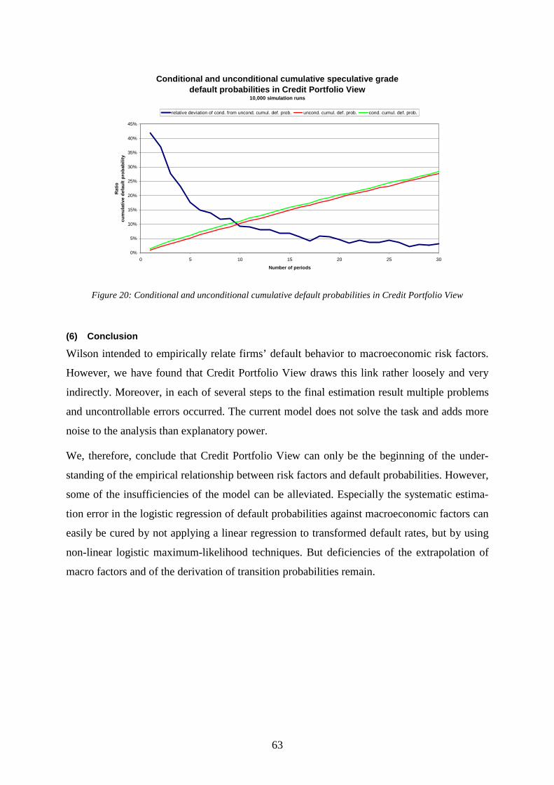
63

Conditional and unconditional cumulative speculative grade default probabilities in Credit Portfolio View


0%

5%

10%

15%

20%

25%

30%

35%

40%

45%

0 5 10 15 20 25 30

Number of periods

Ratio

cum

ulat

ive

defa

ult p

roba

bilit

y

relative deviation of cond. from uncond. cumul. def. prob. uncond. cumul. def. prob. cond. cumul. def. prob.

Figure 20: Conditional and unconditional cumulative default probabilities in Credit Portfolio View

(6) Conclusion

Wilson intended to empirically relate firms’ default behavior to macroeconomic risk factors.

However, we have found that Credit Portfolio View draws this link rather loosely and very

indirectly. Moreover, in each of several steps to the final estimation result multiple problems

and uncontrollable errors occurred. The current model does not solve the task and adds more

noise to the analysis than explanatory power.

We, therefore, conclude that Credit Portfolio View can only be the beginning of the under-

standing of the empirical relationship between risk factors and default probabilities. However,

some of the insufficiencies of the model can be alleviated. Especially the systematic estima-

tion error in the logistic regression of default probabilities against macroeconomic factors can

easily be cured by not applying a linear regression to transformed default rates, but by using

non-linear logistic maximum-likelihood techniques. But deficiencies of the extrapolation of

macro factors and of the derivation of transition probabilities remain.

64

7. Rating based estimation of default probabilities: the CRE model

The last approach to estimate default probabilities of rated companies we would like to pre-

sent is part of the Credit Risk Evaluation model. The CRE model was developed by the author

for the Center for Risk and Evaluation GmbH & Co. KG, Heidelberg.

a) Main concept and derivation of default probability

In order to properly depict the characteristic features of different customer segments, the CRE

model is very flexible in that it allows the use of distinct estimation methods for distinct

groups of clients, which includes firms in different industries and countries and private cus-

tomers.

The CRE model comprehends three empirical influences of client’s default probabilities:

country risk and macro and micro economic influences on clients’ default risk.

(1) Country risk

The default risk of the client’s resident country is an essential factor in the assessment of de-

fault risk because in many cases firms and private customers are prevented from fulfilling

their financial obligations against their own will by purely external reasons.

We define a country’s default as any temporary interruption of money transfers from that

country to the home country of the financial institution that makes the analysis. Disturbances

of money transfers can be due to economical or political reasons such as wars and shortages

of foreign money of the central bank. Numerous such crises could be observed since the

1960’s in Eastern Europe, Asia, Latin and Middle America, and Africa158.

If a financial institution does not make it’s own investigation of country risk, country ratings

and estimates of default probabilities can be obtained from the international rating agencies

such as Moody’s or Standard and Poor’s159.

158 For instance in Argentina, Costa Rica, Iran, Ghana, Guatemala, Indonesia, Uganda, Nicaragua, Zaire, Yugoslavia, Ni-

geria, Panama, Rumania, Uruguay, and others. See UBS (2001), p. 6. 159 Confer to UBS (2001), pp. 5f. Examples for Moody’s and S&P’s country ratings are

Rating Country AAA Germany, France, USA, Switzerland, Austria AA Belgium, Italy, Spain A Greece, Israel

BBB Croatia, Lithuania, Poland, South Africa, Uruguay BB Argentina, Columbia, Mexico B Brazil, Lebanon, Rumania, Turkey, Venezuela

CCC Russia

65

Usually country risk is incorporated into credit risk models in the way that all clients that re-

side in a country are downgraded to the countries’ rating. This means a company in Mexico

(BB) cannot have an A rating, even if it is innovative, competitive, and financially well man-

aged.

This methodology has two disadvantages. Firstly, it cannot further distinguish between clients

who have the same rating as or a higher rating than their country. It is, however, not plausible

that AAA, A, and BB counterparties in Mexico all have the same financial prospects and the

same creditworthiness. Secondly, it does not express the effect that all of a country’s residents

are affected simultaneously by a war or a general financial crisis. This argument shows that

country risk is not only important in terms of default probability, but that it is also a concept

of dependence between counterparties.

For this reason, the state of a country, whether it is financially intact or in default, is treated as

a background factor in the CRE model. A client’s rating is considered as being conditional to

his country being intact. Thus, there can be an A-rated company in a BB country such as

Mexico. If, on the other hand, a country defaults, all clients residing in it automatically de-

fault, too. This setting can incorporate country risk, the differences in credit quality between

risk grades, and the chain reaction declenched by a country default.

The home country of the financial institution that makes the analysis is a special case. This is,

firstly, because its countrymen do not need foreign money to meet their obligations. The

country’s central bank plays no role in this financial relationship. Even if the central bank

runs out of foreign money, clients can pay their liabilities. It is, secondly, because a political

crisis such as a war would directly involve the financial institution, too. This is an exceptional

situation that is not relevant for credit risk management. We, therefore, assume that the bank’s

home country is risk-free and cannot default.

Taking into consideration that countries themselves are strongly interrelated, this understand-

ing can be extended to groups of countries that are closely fraternized with the bank’s home

country. It is, for instance, hardly imaginable that a country that is part of the eurozone can

isolatedly default. Sharing the same currency and exchanging most of their imports and ex-

ports, it is likely that a crisis would quickly spread to the partner countries. For a respective

bank it is, therefore, reasonable to consider the eurozone as its home country.

A segment of customers that needs special attention are big multinational companies that are

well diversified among several countries. If a company has major dependences in other coun-

66

tries, it is entirely possible that it can still meet all of its international obligations even if its

headquarters or another part of it are temporarily cut off. This effect is described in the CRE

model by randomization. This means that if a country defaults occurs, it does not surely

spread to the company, but just with a certain probability.

It is important to note that it is not obligatory to consider country risk in the CRE model. Es-

pecially small regional banks frequently do not have any or very little business abroad. In this

setting, it does not seem necessary to monitor country risk.

(2) Micro economic influences on default risk

If a bank knows its clients’ business relationships and their reasons for default well, it can

take microeconomic influences on default risk into consideration.

Besides the general business risk, companies carry a distinct default risk similar to financial

institutions. The default of a business partner can immediately bring a firm into financial dis-

tress. A prominent example is the evasion of the big construction company Schneider AG in

Germany in 1995. Dozens of smaller construction companies that worked exclusively on the

building sites of the Schneider AG would have had also been drawn into default if the

Deutsche Bank, one of the major creditors of Schneider AG, had not acknowledged its social

responsibility as the leading financial institution in Germany and paid the outstanding debt.

Financial distress can carry over from one company to another mainly for two reasons.

Firstly, a firm can run into liquidity shortages if a relevant part of its short term outstanding

claims cannot be expected to be paid in the near future, if at all. This is a major cause of bank-

ruptcy in the eastern federal states in Germany. Secondly, a firm can loose part of its sales

structure if an important client is lost. It is hit particularly hard, if the market is small and if it

has only a few clients. Both setbacks were the case in the example above. This argument also

shows that economic subjects do not only depend upon each other via systematic risk factors

in the economy as is often said160.

Micro economic influences on default risk can be a valuable tool for the modeling of default

probabilities if a regional economic structure is dominated by only a few large companies.

Industries in which this is frequently the case are the traditional sectors including the steel,

coal, and car industries. For instance, Wolfsburg strongly depends upon Volkswagen, Cler-

mont Ferrand upon Michelin, Longbridge upon Rover, and Bitterfeld upon Leuna and Buna.

A collapse of the major company leads to the sudden unemployment of thousands in the af-

160 Cf. Wilson (1997a,b), Credit Suisse Financial Products (1996)

67

fected region. Many of the dismissed workers will have problems to quickly find a new job so

that mortgage loans and other credits are immediately endangered. Furthermore, many

smaller companies in the area can now only sell fewer goods and might be drawn into the

crises.

Note that similar micro economic relationships can also imply an improvement in a com-

pany’s credit quality if a direct competitor defaults. This phenomenon, however, is probably

of minor weight.

Besides general economic dependencies, an important case of relationships among individual

counterparties is domination due to possession or close financial association. For instance,

companies that belong to the same owner or to the same holding are likely to face financial

difficulties if the holding or the owner defaults. Being obliged to report this kind of affiliation

to the legal banking authorities, banks have well researched data at hand about this special

situation161.

Finally, clients often appear in various roles in a bank’s portfolio. A client can be an obligor

or a trade partner. In this case, his credit risk results from the transactions made with him di-

rectly. On the other hand, the bank can hold a position in a short put option on the client’s

equity. In this case, someone else would be the direct counterparty and the client under con-

sideration is only indirectly involved. However, he originates a credit risk to the bank because

the short put position would drastically increase in value if he defaults. For marginal risk

analysis, pricing, and exposure limitation it makes a great difference whether a client has to

pay and is made responsible for the credit risk that results from his only own transactions or

for the total risk that is incurred by him as a result of direct and indirect financial interactions.

This problem can easily be solved if micro economic relationships are introduced into the

model. Here, the client can be represented by two identical copies that fully depend upon each

other, i.e. they either simultaneously default or survive. Both copies only differ in the amount

of exposure assigned to them and in the stand alone probability of default. The first one corre-

161 See for instance KWG § 19, 2: “1 Im Sinne der §§ 10, 13 bis 18 gelten als ein Kreditnehmer zwei oder mehr natürliche

oder juristische Personen oder Personenhandelsgesellschaften, die insofern eine Einheit bilden, als eine von ihnen unmittelbar oder mittelbar beherrschenden Einfluß auf die andere oder die anderen ausüben kann, oder die ohne Vor-liegen eines solchen Beherrschungsverhältnisses als Risikoeinheit anzusehen sind, da die zwischen ihnen bestehen-den Abhängigkeiten es wahrscheinlich erscheinen lassen, daß, wenn einer dieser Kreditnehmer in finanzielle Schwie-rigkeiten gerät, dies auch bei den anderen zu Zahlungsschwierigkeiten führt. 2 Dies ist insbesondere der Fall bei:

- allen Unternehmen, die demselben Konzern angehören oder durch Verträge verbunden sind, die vorsehen, daß ein Unternehmen verpflichtet ist, seinen ganzen Gewinn an ein anderes abzuführen, sowie in Mehrheitsbesitz stehenden Unternehmen und den an ihnen mit Mehrheit beteiligten Unternehmen oder Personen, (...)

- Personenhandelsgesellschaften und jedem persönlich haftenden Gesellschafter sowie Partnerschaften und jedem Partner und

- Personen und Unternehmen, für deren Rechnung Kredit aufgenommen wird, und denjenigen, die diesen Kredit im eigenen Namen aufnehmen. “

68

sponds to the business done with the client personally, the second stands for the indirect credit

risk he causes. Hence, both sources of risk will remain separated in all subsequent risk

management actions.

Micro economic relationships are modeled by randomization in the CRE model. Given the

default of a client, his business partners fail with certain probabilities. Randomizing weights

can be freely chosen. They can be directly estimated from the bank’s default experience.

Micro economic dependencies between counterparties are typically asymmetric. An employee

usually depends much more on his employer than vice versa. The craftsman is severely af-

fected by the default of the large construction company, while the construction company is

most likely almost independent from the smaller firms that work for it.

It is worth mentioning again that micro economic influences on default risk do not have to be

considered if they are not relevant for the bank’s market segment or if the bank cannot supply

the necessary data.

(3) Macroeconomic influences on default risk

The two influences on default probabilities previously discussed made no explicit use of a

client’s rating. Nevertheless, the rating is a decisive information for the assessment of a coun-

terparty’s future default behavior. In the following, we assume that known cases of default

due to country risk or micro economic relations are left out of the estimation of rating based

default probabilities.

As we already indicated in Figure 8 and the discussion of Wilson’s model, the macroeco-

nomic environment has a significant influence on a portfolio’s default situation. However, the

impact of the current macroeconomic scenario is not the same in all industries and especially

not in all rating grades and customer segments. For instance, a default of a AAA-company has

never been observed within a time horizon of one year, not even in the darkest economic cri-

sis. For this reason, it is impossible to directly estimate systematic influences on the default

probabilities of high grade companies.

Another example is private customers who are not self-employed. They are only indirectly

affected by macroeconomic shocks via their employer. Only if the employing company col-

lapses or if the employee is dismissed, does the economic environment reach the private cus-

tomer.

69

Consequently, it should be possible to not take account of macro factors in the evaluation of

the default behavior of certain customer segments. In the CRE model, the method used to es-

timate default probabilities can, therefore, be independently chosen for each group of clients.

Customer segments can be defined freely by the bank. For high grade firms, for industries that

are not closely integrated into the macroeconomic environment, and for private customers the

mean value model can be used.

In the following, we would like to present the macro model that can be employed in the CRE

model to assess default probabilities of speculative grade firms. The term ‘macro model’ may

be misleading, though, since the CRE model does not contain an explicit prognosis compo-

nent for the development of macroeconomic factors. The forecast of macro factors is a non-

trivial pursuit. Year by year, many highly profiled research institutions in various countries

try in vain to make precise statements about the future unemployment rate, the GDP growth

rate etc. Any attempt to include conjectures about future values of macro factors into a credit

risk model needs to be simplistic and, in fact, misleading.

For this reason, the CRE model employs only values of macro factors that are already observ-

able at the evaluation time to estimate firms’ future default behavior. This approach is in line

with most analyses in the literature, which found that the economic environment influences

the economy’s default situation with a certain time lag162. Hence, the macro data known today

is sufficient to predict a firm’s default behavior over the next 1-3 years. However, it is hardly

possible to make forecasts over longer time horizons. Therefore, the CRE model uses macro

factors only to make short-term predictions of default rates163.

As already mentioned, the impact of the business cycle on firm’s default rates not only de-

pends on their belonging to a certain industry, but also upon their rating. For this reason, the

CRE model does not comprise all speculative grade companies in an industry to a ‘credit risk

indicator’ as in Wilson (1997a) or in Kim (1999) because the inference of rating specific de-

fault probabilities from the indicator is not possible without major additional imprecisions164.

A default has a much greater impact on a client’s or a portfolio’s credit risk than a simple rat-

ing downgrade that leads to a comparably small change in value. Thus, imprecisions particu-

larly need to be avoided in the estimation of default probabilities. The regression of default

162 Cf. the discussion in Bär (2000), Lehment et al. (1997) and others. 163 Long-term prognoses of default probabilities are vague and unreliable at any rate. A simple method to extrapolate one-

year default probabilities to n-year time horizons is to assume defaults to follow a Markov process and multiply the transition matrix n-times with itself.

164 See the discussion of Wilson’s model above.

70

rates against macro factors is, therefore, done for each industry and each speculative grade

rating category separately.

To relate systematic economic factors to firm’s default rates, we propose the following simple

model. Let niYi ,...,1, = be the observed default rates in period i. Let mii XX ,...,1 be the mac-

roeconomic factors explaining the default situation in period i. Taking account of a certain

time lag, mii XX ,...,1 can be observations made in period i - 1 or earlier. The model is then de-

scribed by the equation

Yimimii XXY εβββ ++++= l110

where εYi is an error term with mean zero and unknown, but constant variance σ. We do not

make any distributional assumptions concerning εYi.

The parameters β0,…,βm can be estimated using least squares techniques. This model is

equivalent to the mean value model if β1,…,βm are identically set to zero. All parameter values

can be estimated consistently165.

An important feature of this model is that it does not require the independence of defaults

conditional to a macroeconomic setting166. This is consistent with the larger architecture of

the CRE model since we will assume that sectors can be correlated beyond the macroeco-

nomic influences on default probabilities167. This is a significant advantage with respect to

Credit Risk + where firms in different sectors are necessarily independent and to Credit Port-

folio View where sectors are also independent if the error terms are uncorrelated168.

Due to the direct linear regression, extrapolated values for Yi could respectively be negative or

outside the unit interval. In practice this is not an urgent problem, though, since we don’t in-

tend to simulate error terms. Moreover, it is straightforward to confine Yi to reasonable values

by introducing upper and lower bounds, i.e. if the extrapolated value is negative or below a

certain threshold, the expected default probability is set to the minimal value that is thought

acceptable. However, if the current macroeconomic setting implies an extreme deviation of

estimated default probabilities from their long term mean, this result should be handled with

care because it could indicate that a structural break has occurred and that the validity of the

model needs to be put into question.

165 While the least squares estimator is consistent, it is not necessarily efficient because the error terms are non-normal

and can also be skewed if correlations are positive. Further research has to be done to reduce the variance of the es-timation.

166 This assumption was essential in Credit Portfolio View and Credit Risk+. Without it all estimations are wrong in these models.

167 See section II.A.2 below. 168 A problem which is not discussed in Wilson’s articles.

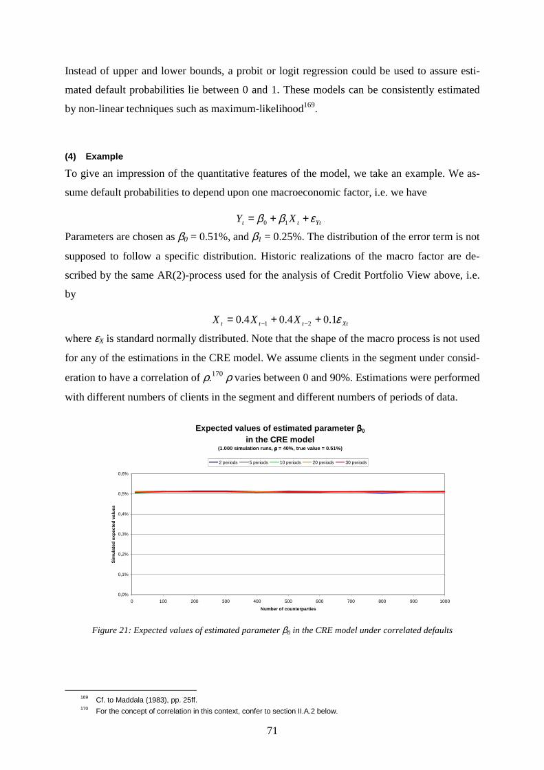
71

Instead of upper and lower bounds, a probit or logit regression could be used to assure esti-

mated default probabilities lie between 0 and 1. These models can be consistently estimated

by non-linear techniques such as maximum-likelihood169.

(4) Example

To give an impression of the quantitative features of the model, we take an example. We as-

sume default probabilities to depend upon one macroeconomic factor, i.e. we have

Yttt XY εββ ++= 10 .

Parameters are chosen as β0 = 0.51%, and β1 = 0.25%. The distribution of the error term is not

supposed to follow a specific distribution. Historic realizations of the macro factor are de-

scribed by the same AR(2)-process used for the analysis of Credit Portfolio View above, i.e.

by

Xtttt XXX ε1.04.04.0 21 ++= −−

where εX is standard normally distributed. Note that the shape of the macro process is not used

for any of the estimations in the CRE model. We assume clients in the segment under consid-

eration to have a correlation of ρ.170 ρ varies between 0 and 90%. Estimations were performed

with different numbers of clients in the segment and different numbers of periods of data.

Expected values of estimated parameter ββββ0 in the CRE model

(1.000 simulation runs, ρρρρ = 40%, true value = 0.51%)

0,0%

0,1%

0,2%

0,3%

0,4%

0,5%

0,6%

0 100 200 300 400 500 600 700 800 900 1000Number of counterparties

Sim

ulat

ed e

xpec

ted

valu

es

2 periods 5 periods 10 periods 20 periods 30 periods

Figure 21: Expected values of estimated parameter β0 in the CRE model under correlated defaults

169 Cf. to Maddala (1983), pp. 25ff. 170 For the concept of correlation in this context, confer to section II.A.2 below.

72

Figure 21 shows the expected estimation results of the mean-value-parameter β0. It is obvious

that the parameter is unbiasedly estimated for any number of counterparties and periods, al-

though defaults are not supposed to be independent, but significantly correlated.

The standard deviation of the estimated parameter value, on the other hand, does depend on

the number of clients and especially on the number of periods of data available, as is to be

expected. However, the informational content in the number of counterparties is quickly ex-

ploited.

Standard deviation of estimated parameter ββββ0 in the CRE model

(1,000 simulation runs, ρρρρ = 40%)

0,0%

0,5%

1,0%

1,5%

2,0%

2,5%

0 100 200 300 400 500 600 700 800 900 1000Number of clients

Estim

ated

sta

ndar

d de

viat

ion


Figure 22: Standard deviation of estimated parameter β0 in the CRE model under correlated defaults

The same observations can be made when we look at the volatility parameter β1.

Expected value of macro parameter ββββ1 in the CRE model

(1,000 simulation runs, ρρρρ

= 40%, true value = 0.25%)

0,00%

0,05%

0,10%

0,15%

0,20%

0,25%

0,30%

0 100 200 300 400 500 600 700 800 900 1000Number of clients

Sim

ulat

ed e

xpec

ted

valu

e

5 periods 10 periods 20 periods 30 periods

Figure 23: Expected value of macro parameter β1 in the CRE model under correlated defaults

73

The estimation is unbiased for any number of clients and periods even if defaults are corre-

lated. Again the parameters standard deviation predominantly depends on the number of peri-

ods.

Standard deviation of estimated parameter ββββ1111

in the CRE model(1,000 simulation runs, ρρρρ = 40%)

0,0%

0,5%

1,0%

1,5%

2,0%

2,5%

3,0%

0 100 200 300 400 500 600 700 800 900 1000Number of counterparties

Estim

ated

sta

ndar

d de

viat

ion


Figure 24: Standard deviation of estimated parameter β1 in the CRE model under correlated defaults

The estimator’s standard deviations are not only related to the number of counterparties and

periods as can be seen in the charts, but also to the degree of correlation among counterpar-

ties. As in the mean value model, standard deviations are relatively large compared to the size

of the respective parameters and increasing in the correlation.

Standard deviation of estimated parameters (ββββ0,ββββ1) in the CRE model dependent on correlations

(300 counterparties, 15 periods, 1,000 simulation runs)

0,0%

0,5%

1,0%

1,5%

2,0%

2,5%

3,0%

0% 10% 20% 30% 40% 50% 60% 70% 80% 90% 100%Correlations

Estim

ated

sta

ndar

d de

viat

ions

β1 β0

Figure 25: Standard deviation of estimated parameters (β0,β1) in the CRE model dependent on the size of corre-lations

74

Figure 26 shows the joint distributions of parameters β0 and β1, clearly illustrating the increas-

ing variability and skewness in the estimation for high correlations171.

Distributions of estimated parameter values (ββββ0,ββββ1) in the CRE model

Standard deviations of joint estimators: σσσσρρρρ = 0 = 0.53%, σσσσ ρρρρ = 0.2 = 1.67%,σσσσρρρρ = 0.4 = 2.76%, σσσσρρρρ = 0.6 = 4.28%, σσσσρρρρ = 0.8 = 7.21%

(1,000 simulated pairs, 30 periods, 500 clients)

-0,25

-0,2

-0,15

-0,1

-0,05

0

0,05

0,1

0,15

0,2

0,25

-1,0% -0,5% 0,0% 0,5% 1,0% 1,5% 2,0% 2,5% 3,0% 3,5% 4,0%Estimated parameter value for ββββ0, true value = 0.51%

Estim

ated

par

amet

er v

alue

for ββ ββ

1, tr

ue v

alue

= 0

.25%

ρ = 0.8 ρ = 0.6 ρ = 0.4 ρ = 0.2 ρ = 0 true value

Figure 26: Distributions of estimated parameter values (β0,β1) in the CRE model under various correlations

Table 5 sums up the main characteristics of the distributions of parameter estimators172. The

similarities to the results in the mean value model are striking. Here again the mean parameter

value is unbiasedly estimated while the uncertainty and also the skewness of the estimation

results increases with correlations. This result holds for both parameters β0 and β1.

β0β0β0β0

ρρρρ

====

0000

ρρρρ

====

0.20.20.20.2

ρρρρ

====

0.40.40.40.4

ρρρρ

====

0.60.60.60.6

ρρρρ

====

0.80.80.80.8

Mean 0,511% 0,514% 0,513% 0,508% 0,527% Std-Dev 0,072% 0,211% 0,383% 0,558% 1,018% Skewness 9,10E-11 9,05E-09 1,10E-07 5,30E-07 6,06E-06 Kurtosis 1,01E-12 1,01E-10 2,23E-09 2,25E-08 8,43E-07

β1β1β1β1

Mean 0,251% 0,259% 0,245% 0,256% 0,260% Std-Dev 0,527% 1,656% 2,738% 4,227% 7,140% Skewness 2,29E-08 3,77E-06 2,62E-05 2,25E-04 5,56E-04 Kurtosis 2,50E-09 5,47E-07 1,17E-05 9,90E-05 7,32E-04 500 clients 30 periods 1,000 simulation runs

Table 5: Characteristics of distributions of parameter estimators (β0,β1) in the CRE model under various corre-lations

171 See also Table 5 below. 172 It should be noted that Table 5 corresponds to Figure 26 and, hence, includes only 1,000 simulation runs. Thus, im-

precisions due to sampling errors may occur, while the general trend seems to be clear.

75

(5) Conditional transition probabilities

The last step in the macro model within the CRE model is the derivation of transition prob-

abilities conditional to the current economic background. Since we have done the estimation

of conditional default probabilities not only for different industries, but also for individual

rating grades, we only have to calculate non-default transition probabilities173.

Similar to Wilson’s approach, we base the derivation of transition probabilities on the ratio of

the estimated conditional default probability to its long-term mean. Precisely, we suggest a

linear transformation of the following form

jn

tnjtj p

ppwp +

−= 1

ˆˆ

for j = 1,…,n, where n is the number of rating grades, np is the estimated long-term mean

default probability of the rating grade under consideration, tnp is the estimated conditional

default probability, jp is the estimated long-term mean probability to migrate from the pre-

sent rating to rating j, tjp is the estimated conditional transition probability, and wj is a sensi-

tivity weight.

Since we have already estimated tnp , we choose nn pw = . The other parameters wj for j =

1,…,n-1, have to be estimated from the bank’s experience. They could, for instance, be chosen

as the least squares estimators of

R∈=

=

+

−−∑

jw

m

ij

n

injij p

ppw min1ˆ !

2

1

π

for grades j = 1,…,n-1, where ijπ is the observed transition frequency to rating j in period i for

i = 1,…,m if there are m periods of data available, and inp is the default probability for period

i interpolated from the estimated values for β0 and β1 above and the observed macroeconomic

factors. Note that for any value of wj the mean of the resulting estimated transition probabili-

ties is equal to jp . This is due to the linear regression model of tnp where the mean of the

estimated default probabilities is always equal to the mean of the observed default frequen-

cies174.

173 Credit Portfolio View, on the other hand, has to derive individual default and transition probabilities from the pool of

speculative grade firms in an industry for all rating grades.

174 XY 10 ββ += is one of the equations to be solved in the least squares estimation.

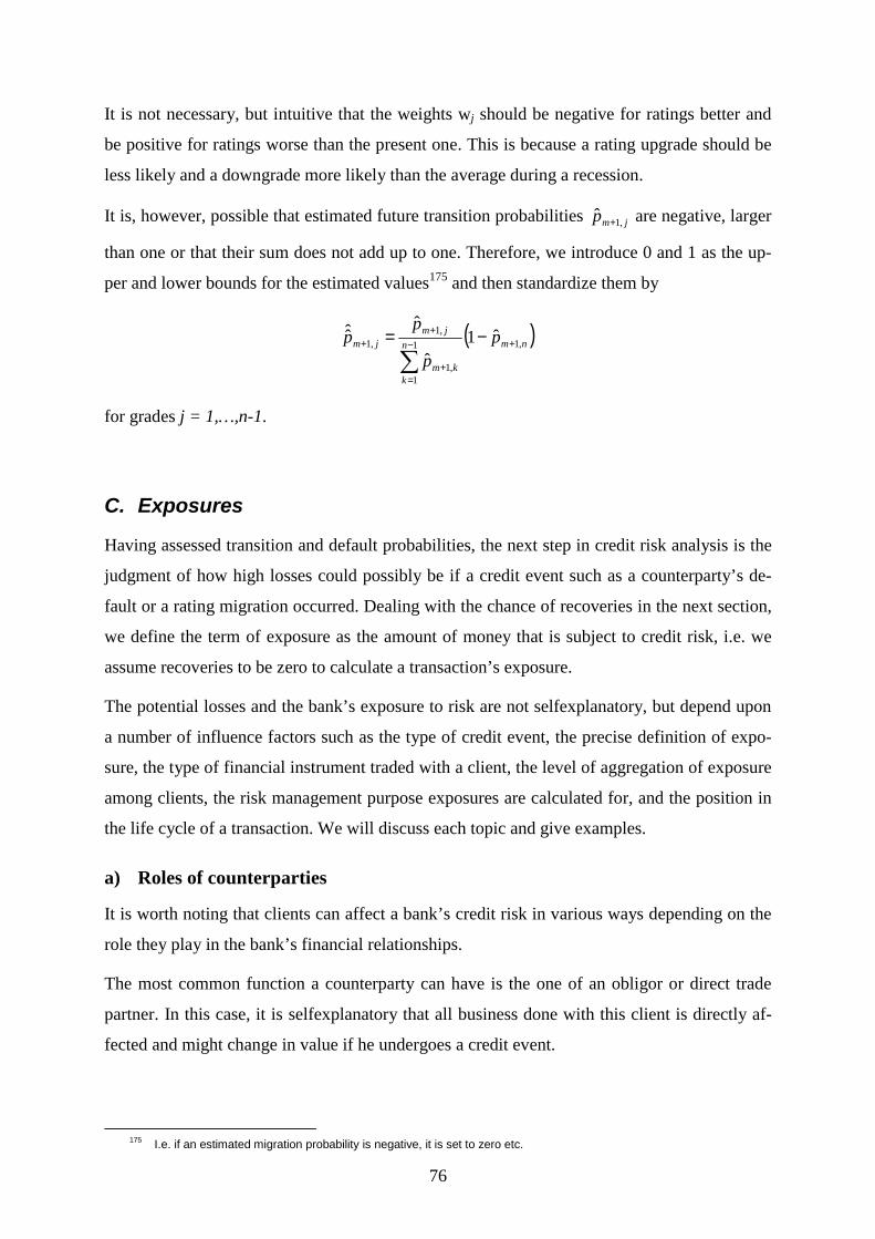
76

It is not necessary, but intuitive that the weights wj should be negative for ratings better and

be positive for ratings worse than the present one. This is because a rating upgrade should be

less likely and a downgrade more likely than the average during a recession.

It is, however, possible that estimated future transition probabilities jmp ,1ˆ + are negative, larger

than one or that their sum does not add up to one. Therefore, we introduce 0 and 1 as the up-

per and lower bounds for the estimated values175 and then standardize them by

( )nmn

kkm

jmjm p

p

pp ,11

1,1

,1,1 ˆ1

ˆ

ˆˆ+−

=+

++ −=

∑

for grades j = 1,…,n-1.

C. Exposures

Having assessed transition and default probabilities, the next step in credit risk analysis is the

judgment of how high losses could possibly be if a credit event such as a counterparty’s de-

fault or a rating migration occurred. Dealing with the chance of recoveries in the next section,

we define the term of exposure as the amount of money that is subject to credit risk, i.e. we

assume recoveries to be zero to calculate a transaction’s exposure.

The potential losses and the bank’s exposure to risk are not selfexplanatory, but depend upon

a number of influence factors such as the type of credit event, the precise definition of expo-

sure, the type of financial instrument traded with a client, the level of aggregation of exposure

among clients, the risk management purpose exposures are calculated for, and the position in

the life cycle of a transaction. We will discuss each topic and give examples.

a) Roles of counterparties

It is worth noting that clients can affect a bank’s credit risk in various ways depending on the

role they play in the bank’s financial relationships.

The most common function a counterparty can have is the one of an obligor or direct trade

partner. In this case, it is selfexplanatory that all business done with this client is directly af-

fected and might change in value if he undergoes a credit event.

175 I.e. if an estimated migration probability is negative, it is set to zero etc.

77

However, an economic subject can also be indirectly related to a bank’s portfolio, for instance

as an issuer of stock or bonds if the bank has bought or sold derivatives that have these securi-

ties as an underlying asset. Here it might happen that the direct counterparty has a steady

credit quality while the value of the derivative considerably alters due to a deterioration or

improvement in the credit worthiness of the issuer of the underlying asset.

Especially short put options on stock and bonds carry an extreme credit risk which is attached

to the indirectly involved counterparty. Put options experience their maximum increase in

value if the value of the underlying asset breaks down. In the case of a default of the counter-

party, a put is sure to be exercised. Hence, a future default of the issuer of the underlying in-

curs an (additional) loss that is equal to the actual value of the underlying asset.

This shows that the often heard statement that liabilities are not subject to credit risk is not

true since it may happen that the size of a liability changes owing to a credit event that might

be caused by an indirect counterparty. The indirect counterparty risk even makes up for 80-

90% of most banks’ default risk in trade portfolios. However, always being a liability towards

the direct counterparty, a short put position does not carry a credit risk with regard to him

because his default would not protect the bank from having to pay its obligations if his posi-

tion is taken by one of his creditors.

This is different in case of long option positions. Here we have two sources of credit risk, one

due to the direct counterparty as long positions are always assets and the second one due to a

deterioration in credit quality of the issuer of the underlying asset which can also be referred

to as a special interest rate or a special equity price risk.176

Although tied to the same probability of default, both types of counterparty risk should be

well distinguished in credit risk management because a client has in general no influence on

the size of the exposure or risk that he entails as an indirect counterparty. If both types of risk

are mixed, his credit line, for instance, could quickly be used up for no reason apparent to

him.

b) Concepts of exposure

A major complication in the calculation of exposures is to find a concept that applies to all

kinds of financial products consistently and can be used to express the consequences of a de-

fault.

176 See for instance Grundsatz 1, § 23 and § 25.

78

Traditionally, credit products such as bonds and loans were accounted for by their book value

and derivatives by their notional. Both concepts have two fundamental disadvantages. Firstly,

they are not related to the actual market situation. Changes in market prices and interest rates

do not affect a swaps principal or a loans book value. They may, however, significantly influ-

ence their market value and their replacement costs. Secondly, both definitions tend to over-

state the instruments’ true potential loss. This is especially striking for derivative products

where the notional often has no direct relationship to a contract’s value.

A first guess for a better measure of exposure in case of default would be the trade’s

(1) Present value

A deal’s present value177 has the advantage that it is no longer static and keeps track of the

development of market prices. However, some derivative positions such as swaps, FRAs, fu-

tures and short option positions can take on negative values. As already mentioned above,

liabilities are not affected by the default risk of the direct counterparty. This means that trades

with negative present values are not in danger of being lost because a creditor in default

would hand the claim on to his own creditors. Hence, we render the measure of exposure

more precise and define the

(2) Current exposure

A transaction’s current exposure C is the positive part of its present value V, thus,

).,0max( VC =

The current exposure is generally used for fixed income products that are relatively stable in

value such as loans and bonds. In addition to that it has many applications in the management

of spot and short term credit risks where no great changes in present value are to be expected

also for more volatile transactions as, for instance, the replacement risk for newly closed

trades.

The replacement risk178 is the risk that a transaction that has been agreed upon will not be

realized. No party has made any payments. In the case that the transaction is canceled, the

resulting loss is equal to the costs caused if the same trade has to be closed again. This is the

177 Although only approximately equal, we use the terms of present value and market value synonymously throughout this chapter. Especially in the examples we will neglect the transactions’ default risk. This leads to a slight overstatement of the resulting exposures. It seems to be a suitable simplification, though, because, being merely an input for limita-tion, equity allocation, and portfolio management, exposures do not need that degree of precision that is required for pricing, for instance.

178 This risk is also known as “Wiedereindeckungsrisiko“.

79

difference between the transactions current present value and the agreed price. Thus, if the

transaction has risen in value, the exposure is positive and it is zero otherwise.

Similar to the replacement risk is the risk that occurs in the same setting if payments had al-

ready been made and the delivery of the security remains outstanding179. Here the exposure is

equal to the present value of the outstanding delivery180.

The third spot risk where the concept of current exposure can be applied is the risk that pay-

ments or deliveries that are due do not occur while the own party has not taken any action

yet181. It is identical to the replacement risk with the difference that it includes transactions

that have already been taken182.

(3) Examples

To illustrate the notions of present value and current exposure, take a long equity call option

position and a long FRA position as examples.

Let us suppose the equity call to mature in 1 year with a strike price of 100 €. The one-year

risk free interest rate is equal to 6% and the actual equity price is 80 € with an annual volatil-

ity of 1. Then, following the Black-Scholes analysis, the option’s present value is equal to

Voption = 26.67 €

and, thus, the current exposure is as well. Note that a long option position is a right to some-

thing without any obligation once the option premium has been paid. In such a case, the pre-

sent value and the current exposure are always identical.

This is different in case of a forward rate agreement (FRA). A long position in a FRA is the

agreement to grant a credit at fixed conditions at some point in the future. Apparently, the

sign of its market value depends on the market conditions. If interest rates go down, a long

FRA position has a positive market value. If interest rate rise, its value is negative.

Let us again suppose the one-year interest rate is equal to 6% and assume that the interest rate

for 15 months is equal to 6.5% in continuous compounding. The FRA was closed 6 months

ago and is the agreement to grant a loan of 100,000 € over a period of three months beginning

in one year from now at the rate of 8.2%. Thus, its present value is equal to

179 In German this risk is also called “Vorleistungsrisiko”. 180 Cf. Grundsatz 1, § 27.1.2. 181 In German this risk is also called “Abwicklungsrisiko”. 182 Cf. Grundsatz 1, § 27.1.1.

80

( ) 61.70000,100 1%625.1%5.625.0%2.8 −=−= ⋅−⋅−⋅ eeVFRA €

and its current exposure is zero.

(4) Potential exposure

While derivatives are relatively stable in value over short terms, this may not be the case if

longer time horizons are considered, which is usually the case in credit risk management. For

this reason, the concept of current exposure is found unsatisfactory for applications such as

portfolio management and exposure limitation. In terms of credit risk it is particularly prob-

lematic if a counterparty defaults when a transaction or a portfolio performs well in value due

to favorable market conditions. Thus, the credit risk increases in times of hausse and de-

creases during a baisse, and, consequently, concepts of potential exposure183 try to capture the

effects of positive market behavior.

(5) Potential exposure of individual transactions or peak exposure

A typical definition of a position’s potential or peak exposure is a possible value that will not

be exceeded with a probability of say 95%, i.e. the transaction’s potential exposure is an up-

per percentile of its value. It can be found by simulation of its underlying market factors or by

analytic formulas depending on the trade’s structure.

(6) Examples

If we consider the equity option already mentioned above, it is implied by the risk neutral

valuation argument and the general distributional assumptions in Black-Scholes’ theory that

the equity value is lognormally distributed with

( ) ( )

−+Ν TTrSST

22

0 ,2

ln~ln σσ

where St is the equity value at time t, r is the risk free interest rate, and σ is the stock’s annual

volatility.

Thus, the option’s potential exposure follows from the normal distributions percentile. The

95%-percentile, for instance, is equivalent to a deviation of 1.64 standard deviations from the

mean. Hence, we have a potential exposure of

183 Notions of potential exposure are often referred to as ‘credit equivalents’.

81

( ) 18.15764.12

lnexp2

0)( =

−

⋅+

−+= −− XTTrSeP tTr

option σσ €

for the option, where X is the strike price. Note that this value is 5.89 times the option’s pre-

sent value or current exposure.

To calculate the 95%-potential exposure of the long FRA position, we make the distributional

assumptions of Black’s interest rate model, i.e. we suppose the underlying forward rate to be

lognormally distributed with

− TTrNr ff

T2

2

0 ,2

ln~ σσ

where ftr is the underlying forward rate at time t, T = 1 is the time to the granting of the

credit, and σ is its annual volatility. We assume σ = 0.05. Since the value of the long FRA

position is increasing if the interest rates decrease, the upper percentile of the value of the

FRA is equal to the respective lower percentile of the forward rate. Thus, we have for the

95%-percentile of the forward rate

%82.764.12

lnexp2

0 =

⋅−−= TTrr ff

T σσ

implying a ‘long term’ interest rate of

( ) %37.6*

*1

2 =−⋅+=T

TTrTrrf

T

with T* being the maturity of the future credit, and a potential exposure for the FRA of

( ) 71.89000,100 1%625.1%37.625.0%2.8 =−= ⋅−⋅−⋅ eePFRA €.

Four things are worth noting. Firstly, the FRA’s potential or peak exposure is positive al-

though its present value is largely negative and its current exposure is zero. This clearly

shows that the definition of potential exposure as a percentile of the assets’ value distributions

somehow captures extreme market movements. The concept of peak exposure can find a

credit risk even though we expect losses most of the time due to market risk, in our example

with a probability of 88.2%.

Secondly and similarly, the notion of potential exposure tends strongly to the opposite direc-

tion from market risk analysis. If it is used for capital adequacy purposes, it is very likely that

82

too much equity is supplied if market and credit risk are added because they cannot always

occur simultaneously by definition of the amount at stake.

Thirdly, the example of the forward rate agreement shows that the calculation of potential

exposure requires more complicated models than the mere valuation of assets. Since the value

of a FRA only depends on expected interest rates which are implied by the spot interest rate

curve, its valuation can already be done if these elementary data are known. The potential

exposure, however, results from a statement about how far future market factors might move

away from their present position. Therefore, it demands distributional assumptions.

Fourthly, as indicated by the example of the equity option, a transaction’s peak exposure can

be relatively large compared to its current exposure even if the current exposure is already

positive, in the illustration it was more than five times the size. Thus, the sum of all potential

exposures can be considerable put side by side with the value of the respective portfolio.

Moreover, since all transactions are treated isolatedly, impossible combinations can occur,

e.g. a put and a call option that depend upon the same underlying asset move inversely in

value. The potential exposure of the sum of both will, therefore, generally tend to be smaller

than the sum of the potential exposures of the individual transactions.

These arguments imply that the concept of potential exposure should not be used in portfolio

management in order to avoid an unnecessary exaggeration of the amount at stake. It can,

however, be used in exposure limitation where diversification within a portfolio is not of in-

terest and where the diversity of financial products in a client’s subportfolio can be supposed

to be small since banks usually do not hedge a portfolio’s market risk on a client level. But

even here the overstatement of the bank’s exposition to risk would be considerable if expo-

sures are aggregated over several levels up to the full portfolio.

(7) Potential exposure on a portfolio level

A much more moderate concept of potential exposure can be obtained if transactions’ changes

in exposition are calculated on a portfolio level. The calculation proceeds in several steps:

1. The total portfolio is segregated into subportfolios containing transactions with a rela-

tively homogenous time to maturity184.

2. The joint development of underlying market factors is simulated.

184 The accuracy of the calculation can be increased if the portfolio is further subdivided by the type of the market factors,

i.e. equity products are separated by interest rate products etc.

83

3. After each simulation run all trades’ individual current exposures are calculated and added

resulting in a distribution of current exposures for the respective subportfolio.

4. The excess of the desired percentile πα of the exposure distribution over the subportfolios

current exposure CPortfolio to the sum ΣPrincipalsof all transactions’ principals times the indi-

vidual transaction’s principal θPrincipal plus the transaction’s present value Vθ

is the estima-

tor of the transaction’s potential exposure Pθ if it is positive. Otherwise it is zero.

+⋅Σ−

=

−

−−

0,max PrPr

θα

θ θπ

VC

P

onAdd

basisonAdd

incipal

factoronAdd

incipals

Portfolio

For high percentiles πα it can be assumed that the add-on factor is positive. Sometimes the

transaction’s present value Vθ is replaced by its current exposure Cθ as the add-on basis

assuring that the sum of add-on and Cθ is positive so that the max-function is not

needed185. The add-on basis θPrincipal varies depending on the type of the trade. For a long

option position it is the underlying asset to be received or delivered, for a swap it is the

notional of the fictitious underlying bond, etc..

(8) Example

As a simple example to illustrate the concept, we take a portfolio consisting of 100 long eq-

uity call options on 100 different shares having a strike of 100 € and a time to maturity of 1

year. We assume that each share presently is traded at 80 € and has an annual volatility of 1.

All shares’ returns are lognormally distributed with a homogenous correlation of ρ.

185 This is, for instance, the case in the legal exposure calculation method prescribed by the banking supervision authori-

ties, cf. Grundsatz 1 § 10.

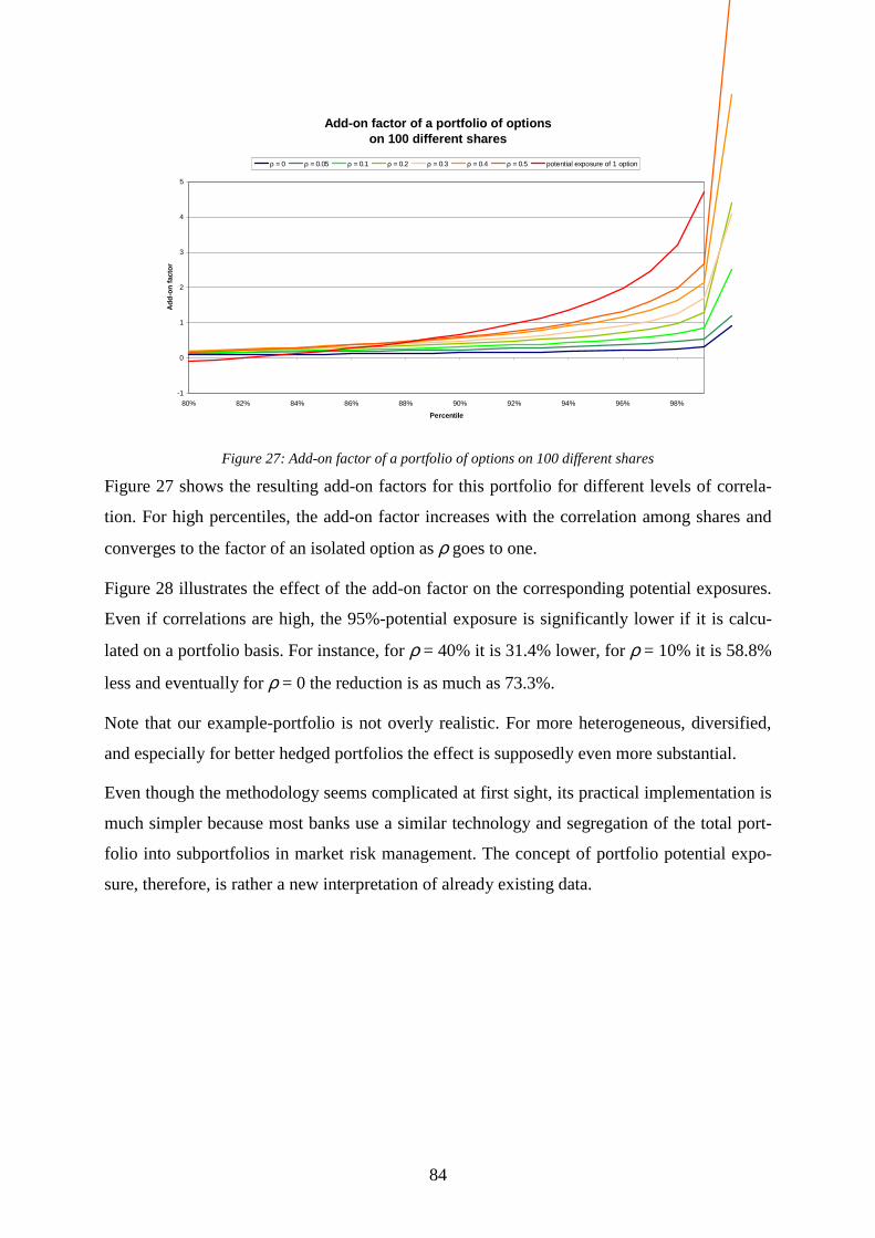
84

Add-on factor of a portfolio of options on 100 different shares

-1

0

1

2

3

4

5

80% 82% 84% 86% 88% 90% 92% 94% 96% 98%

Percentile

Add

-on

fact

orρ = 0 ρ = 0.05 ρ = 0.1 ρ = 0.2 ρ = 0.3 ρ = 0.4 ρ = 0.5 potential exposure of 1 option

Figure 27: Add-on factor of a portfolio of options on 100 different shares

Figure 27 shows the resulting add-on factors for this portfolio for different levels of correla-

tion. For high percentiles, the add-on factor increases with the correlation among shares and

converges to the factor of an isolated option as ρ goes to one.

Figure 28 illustrates the effect of the add-on factor on the corresponding potential exposures.

Even if correlations are high, the 95%-potential exposure is significantly lower if it is calcu-

lated on a portfolio basis. For instance, for ρ = 40% it is 31.4% lower, for ρ = 10% it is 58.8%

less and eventually for ρ = 0 the reduction is as much as 73.3%.

Note that our example-portfolio is not overly realistic. For more heterogeneous, diversified,

and especially for better hedged portfolios the effect is supposedly even more substantial.

Even though the methodology seems complicated at first sight, its practical implementation is

much simpler because most banks use a similar technology and segregation of the total port-

folio into subportfolios in market risk management. The concept of portfolio potential expo-

sure, therefore, is rather a new interpretation of already existing data.

85

Potential exposure of a portfolio of options on 100 different shares

0

50

100

150

200

250

300

350

400

450

80% 82% 84% 86% 88% 90% 92% 94% 96% 98%

Percentile

Pote

ntia

l exp

osur

eρ = 0 ρ = 0.05 ρ = 0.1 ρ = 0.2 ρ = 0.3 ρ = 0.4 ρ = 0.5 potential exposure of 1 option

Figure 28: Potential exposure of a portfolio of options on 100 different shares

(9) Mean expected exposure

Another exposure type is called mean expected exposure. It is defined as the mean of the ex-

pected current exposure of a transaction until maturity or

( )∫=

=T

t

dttVT

M0

)0,)(max(1 E

where T is the time to maturity, V(t) the trade’s present value at time t, and E the expectation

operator. Instead of future market movements the mean expected exposure puts the focus on

the time value of a transaction.

Options, for instance, have a negative time value if market conditions remain unchanged. A

long equity call as in the example above only has a mean expected exposure of 15.64 € com-

pared to a present value of 26.67 €, implying that the mean expected exposure is smaller that

the current exposure. This does not seem convincing for most applications since options and

similar derivatives are explicitly not made for stable markets.

However, the concept of mean expected exposure can well be used for fixed income products

such as bonds, loans, or swaps. This can best be demonstrated by an example. Let’s assume a

flat interest rate curve at 6% and a step-up bond that also pays 6% p.a.. The bonds current

principal is 500,000 € stepping up to 1,000,000 € in 6 months. Principal plus interest will be

repaid in 1 year.

86

As the bond’s interest is conform to the market, it is exactly worth par. Thus, its present value

is equal to

V = 500,000 €.

The mean expected exposure can be calculated as

000,750000,000,1000,5001

2/1

2/1

0

=+= ∫∫== tt

dtdtM €.

For a bond the mean expected exposure seems to be a reasonable concept because, if the bond

defaults in more than 6 months, a much larger amount of money is expected to be lost than its

current exposure.

(10) Maximum exposure

Similar to the mean expected exposure is the maximum exposure. It is defined as

( )( )0,)(max tVMAXTt

E≤

= .

It can well be applied for fixed income products, especially for limitation if a bank wants to

take account of peak exposures and stabilize the employment of credit limits.

(11) Artificial spread curves

For most loans and bonds on the banking books no market prices exist because the secondary

markets for these instruments are highly illiquid as a result of default risk problems which

cause market intransparency. For this reason, usually the trades’ book value is employed for

credit risk management purposes. This leads to valuation inconsistencies, though, because an

instrument’s book value typically deviates from its present or market value. However, if risk-

free interest rates and the client’s default probabilities are known, risk adjusted spread curves

can be derived and the loan’s exposure can be calculated.

Let us take a 2-year loan as an example with a book value or notional of K = 100,000 € and a

fixed interest of r = 10% p.a.. Interest is paid once a year. The client’s first year default prob-

ability has been assessed as p1 = 0.6% and his second year’s was found equal to p2 = 0.4%.

His recovery rate, in case of default, is assumed to be fixed at RR = 50%. The risk-free inter-

est rate is r1 = 4.5% for one and r2 = 5% for two years.

We begin with the calculation of a 2-year risky spread curve. A zero bond that pays out 1 € in

one year and that was closed with the client is worth

87

111111 sr

defaultdefaultno

r eRRppe −−

−

− =

⋅+−⋅

which implicitly defines the 1-year spread s1. Thus, we have

%3.01ln 111 =

⋅+−−=

−NMLNML

defaultdefaultno

RRpps

Analogously the 2-year spread s2 is

( )( ) ( )( )( ) %25.011111ln21

21212 =

⋅−−−+−−−=

−

defaultdefaultno

RRpppps .

We can now value the loan

( ) 95.566,108)1( 22211 =⋅++⋅⋅= ⋅+−−− srsr KereKrV €.

c) Overview over applications

To sum up what was said about the applications of exposure concepts, we give an overview in

Table 6.

Portfolio management Limitation

Equity allocation

Present value O O O Current exposure + O + Peak exposure - + - Portfolio potential exposure ++ ++ ++ Mean expected exposure ++ ++ ++ Maximum exposure - + -

Table 6: Typical applications of exposure concepts

D. Loss and Recovery Rates

One of the major factors of uncertainty in credit risk management is the loss of exposure con-

ditional to default or, conversely, the recovery conditional to default. It is clear that the credit

risk of a contract would be zero even if its default probability is high if its loss conditional to

88

default were zero. On the other hand, its credit risk would reach its maximum if its loss rate

were 100%.

In the following, we will refer to the proportion of the exposure that is lost conditional to de-

fault as loss rate λ, and on the respective recovered proportion as recovery rate r. Both quanti-

ties are related by the equation

r = 1 – λ.

1. Influence factors

Empirical investigations186 have shown that loss and recovery rates are particularly dependant

upon four factors:

1. The concept of default. If the definition of default187 chosen is strict, i.e. if it is an ab-

sorbing state that implies the insolvency of the counterparty or counterparties owning

a contract, recovery rates are lower on average than in case of a weak comprehension

of default where the state is not absorbing. In this second situation many contracts

formerly in default are finally fulfilled and not liquidated prematurely meaning that no

loss occurs at all.

2. The seniority ranking of debt. All kinds of transactions do not have the same priority

or seniority if the assets of a counterparty in insolvency are liquidated and the pro-

ceeds are used to repay the obligations to the counterparty’s creditors. On the contrary,

there is a well defined hierarchy of privileges188 that regulates the sequence in which

claims are satisfied in a liquidation process. The higher a contract’s seniority ranking

is, the higher ceteris paribus is the recovery. Table 7 gives an impression of the effect

of a transaction’s seniority on recovery rates.

SeniorityMean Recovery

(% of face value)Senior secured 63.45%Senior unsecured 47.54%Senior subordinated 38.28%Subordinated 28.29%Junior subordinated 14.66%

Table 7: Mean default recovery rates on public bonds by seniority189

186 Cf. e.g. to Altman et al. (1996), Standard & Poor’s (1992), and Moody’s (1997). All those studies put the focus on US

or multinational companies. We are not aware of a similar study for European companies or for private customers. 187 See above section Definitions of default on page 16. 188 Cf. to Caouette et al. (1998), p. 206, for details. 189 See Moody’s (1997), exhibit 5.

89

3. Instrument type. The impact of the instrument type on recoveries is a consequence of

the instruments’ difference in seniority. Usually, derivative transactions as a whole

have the most junior ranking being only senior to equity. Thus, a company’s share-

holders only receive a recovery if all other of the company’s creditor’s could be paid.

The argument also shows that results as quoted in Table 7 for public bonds can not be

transferred to other product types.

4. Industry of the obligor. A company’s asset structure and especially the assets’ liquida-

tion value strongly depend upon the industrial sector an obligor belongs to. Caouette et

al.190 quote a working paper by Altman and Kishore in which it is found that in the US

the chemical industry (63%) and the public utilities sector (70%) have the highest av-

erage recovery rates while most other industries range around 30-40%. The lodging,

hospital and nursing facilities only have a mean observed recovery rate of 26%.

2. Random Recoveries

Rating agencies usually not only publish mean recovery rates for different seniority classes of

bonds, but also their standard deviation because the uncertainty in recovery rates observed in

different cases is considerable even within the same seniority ranking. However, the knowl-

edge of the recovery rates’ standard deviation renders it possible to take account of this uncer-

tainty and to understand them as a random variable. For convenience rather than for empirical

reasons, the beta distribution is frequently chosen as a model for recovery rates since it can be

fitted by its mean and standard deviation, only takes values between zero and one, and can

easily be simulated by inversion of the cumulative distribution function.

Beta distributions of recovery rates of public bonds in different seniority classes

0

1

2

3

4

5

6

0 0.1 0.2 0.3 0.4 0.5 0.6 0.7 0.8 0.9 1

Recovery Rate

Den

sity

Senior secured Senior unsecured Senior subordinated Subordinated Junior subordinated

Figure 29: Beta distributions of recovery rates of public bonds in different seniority classes191

190 Caouette et al. (1998), p.211. 191 See Moody’s (1997), exhibit 5.

90

Figure 29 gives an impression of the shape of the densities of the resulting beta distributions

of recovery rates if they are fitted with the estimated moments of the distribution192.

Since the seniority ranking is a feature of the single contract, the corresponding recovery rates

cannot be directly used if all transactions belonging to a specific client are considered as one

exposure and a subportfolio that defaults simultaneously. Therefore, an aggregation rule is

required in this situation:

Let X1,…, Xn be the exposures of the single transactions in the subportfolio that is owned by

the counterparty under consideration with expected recovery µi and standard deviation σi for i

= 1,…,n. Let

∑=

= n

jj

ii

X

X

1

α

for i = 1,…,n, be the share of the ith transaction in the exposure of the subportfolio. Then the

mean recovery µ of the subportfolio can be calculated as

∑=

⋅=n

iii

1µαµ

and the standard deviation σ as

∑=

⋅=n

iii

1σασ

since the recoveries can be assumed to be fully dependent because they refer to the same

counterparty.

Note that the resulting distribution would not necessarily be a beta distribution again if the

distributions of the single recovery rates are beta. This is not a serious problem, though, since

the assumption of a beta distribution was arbitrary. Therefore, it is conceptually no difference

if only the resulting distribution is assumed to be beta.

192 The beta distribution with parameters a and b has the density function

11, )1(

)()(

)()(

−−−

Γ⋅Γ

+Γ=

baba xx

ba

baxf .

where ( )⋅Γ is the gamma function. The parameters are related to the mean µ and the standard deviation σ by

( )µ

σ

µµ−

−=

2

21

a and ( ) ( )µσ

µµ−−

−= 1

12

2

b .

91

3. Practical problems

The valuation of assets after a default is not straight forward since for most ‘used’ assets the

market is highly illiquid so that just book values, but no market prices exist. Moreover, a full

settlement after an insolvency usually takes years so that definite results about losses and re-

coveries cannot be obtained quickly. A practical compromise has turned out to be relatively

accurate is to estimate the value of recoveries one month after default193.

Finally, the legal environment can have a major impact on recovery rates. This implies that

the results of recovery studies for the US cannot easily be transferred to European situations

and underlines the need for investigations for countries outside the US.

E. Pricing

An important component in the management of a single client’s credit risk is the correct and

risk adequate pricing of new transactions. The pricing ensures that the client himself pays for

the expected cost that the financial institution has to carry when the transaction is agreed

upon. This includes the refinancing costs and the cost of risk, i.e. the expected loss of the

trade and the costs of provisions for the unexpected loss.

As examples for the general methodology, we will derive pricing formulas for a fixed rate

bond as an interest rate product and for a European equity call option. For simplicity, we will

ignore the possibility of rating transitions and only consider the two states of default and no

default as influences of the client’s credit risk on the value of the product.

1. Pricing of a fixed rate bond

A fixed rate bond is a loan over a certain number of periods of time at a fixed rate. At the end

of each period the accrued interest and an amortization are paid194.

As an example, we take a loan of 1,000 € over five years where 5 annuities are paid at a rate

of 6% plus an amortization of 200 € at the end of each year. The development of the notional

of this bond has the following structure:

193 Cf. Gupton et al. (1997), p. 77. 194 Note that the amortization can be positive or negative. If it is negative, we also speak of a step-up bond.

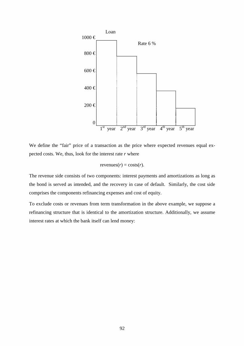
92

Loan 1000 €

800 €

Rate 6 %

600 €

400 €

200 €

0

1st year 2nd year 3rd year 4th year 5th year

We define the “fair” price of a transaction as the price where expected revenues equal ex-

pected costs. We, thus, look for the interest rate r where

revenues(r) = costs(r).

The revenue side consists of two components: interest payments and amortizations as long as

the bond is served as intended, and the recovery in case of default. Similarly, the cost side

comprises the components refinancing expenses and cost of equity.

To exclude costs or revenues from term transformation in the above example, we suppose a

refinancing structure that is identical to the amortization structure. Additionally, we assume

interest rates at which the bank itself can lend money:

93

Loan Theoretical refinancing structure 1000 €

800 €

Rate 6 % 1 year, 4 %

200 €

600 €

2 years, 4.5 % 200 €

400 €

3 years, 5 % 200 €

200 €

4 years, 5.20 % 200 €

0

5 years, 5.50 % 200 €

1st year 2nd year 3rd year 4th year 5th year

For the ease of presentation, we fix the following notation:

• Let pi be the probability that the client defaults in year i for i = 1,…,n, given that he

has not defaulted before. For the example we assume: p1 = 1%, p2 = 1.5%, p3 = 1.2%,

p4 = 1.8%, p5 = 1%.

• Let fir be the bank’s reference interest rate for a straight bond with annual coupon

payments with a maturity at the end of year i for i = 1,…,n. In our example, we have: fr1 = 4%, fr2 = 4.5%, fr3 =5%, fr4 =5.2%, fr5 = 5.5%.

• Let *ir be the risk free interest rate of a zero bond with maturity at the end of year i for

i = 1,…,n. For simplicity we assume *ir = f

ir for i = 1,…,n, in the example.

• Let ci be the bond’s notional capital in year i for i = 1,…,n. In the example, we have c1

= 1000€, c2 = 800 €, …, c5 = 200 €.

• Let ai be the amortization at the end of year i for i = 1,…,n. ai = 200 € for all i in the

example.

• Let RR be the client’s expected recovery rate.

94

• Let q be the fraction of the respective notional195 that has to be ensured by equity. We

assume that q is constant over time. A supposition that can easily be relaxed. For the

moment, we presume q as exogenously given.

• Let re be the return on equity intended by the bank. We assume that the bank invests

its equity in risk-free long term tradable bonds where it receives an annual interest rate

of r* to reduce opportunity costs. For the example, we choose re = 15% and r* = 8%.

• We assume that the counterparty can only default right before an interest payment be-

cause in this situation the default incurs the maximum loss due to the accrued interest.

The following theorem then defines the fair risk premium:

Theorem 1: With the above notation the fair price of a fixed rate bond is given as the solution r of the

equation

( ) ( ) ( ) ( )

( )( ) ( ) ( ) 011

1

111

11

1 1**

*

1

1

1*

1*

=

++

+⋅+−⋅−

++⋅⋅−+

++⋅−

∑ ∑

∑ ∏∏

= =

=

−

==

n

i

i

ji

i

ij

i

fi

ei

n

i

i

ji

i

iij

i

ji

i

iij

ra

rrrrqa

rrcRRpp

racrp

Proof:

Let’s look at the income side first:

At the end of year i two kinds of cash flows are expected: an interest plus an amortization

payment. The probability that the cash flows are carried out as intended is equal to the prob-

ability that the client has not defaulted yet, thus, ( )∏=

−i

jjp

1

1 . Hence, the expected value of the

cash flows in year i is

( )( )∏=

+⋅−i

jiij acrp

1

1 .

This amount has a present value of

195 According to Grundsatz 1 § 6.1.1. the amount of equity to be allocated to compensate for the bond’s default risk is a

fraction of its notional. Alternatively, one could supply equity as a fraction of the bonds present value. In this case, a similar formula as in Theorem 1 would result.

95

( ) ( )∏= +

+⋅−i

ji

i

iij

racrp

1*1

1 .

If the counterparty defaults in year i, the exposure ci(1+r) is put into question. According to

our assumptions a present value of

( )ii

irrcRR*1

1++⋅

can be recovered. The probability that the client defaults in year i equals ( )∏−

=

−1

1

1i

jij pp .

We, therefore, have a total expected revenue of

( ) ( ) ( ) ( )∑ ∏∏=

−

==

++⋅⋅−+

++⋅−

n

i

i

ji

i

iij

i

ji

i

iij

rrcRRpp

racrp

1

1

1*

1* 1

111

1 .

The cost function can be developed analogously:

We look at each part of the refinancing structure separately. For all i, the part with maturity at

the end of year i has the same notional as the respective amortization. The whole amount that

is handed out to the client is refinanced over the capital market. However, a fraction q of the

notional has to be provided in form of equity to compensate for the client’s default risk. Thus,

this fraction has to earn the excess return on equity or the risk premium the bank intends.

Hence, each year for year 1 to i nominal interest payments of ( )( )fi

ei rrrqa +−⋅ * are due.

Discounted and aggregated over the years we have

( )( ) ( )∑= +

⋅+−⋅i

jj

i

fi

ei

rrrrqa

1*

*

11 .

Finally, the amortization has to be paid back each year, ( )ii

i

ra

*1+. Altogether the cost function

is given by

( )( ) ( ) ( )∑ ∑= =

++

+⋅+−⋅

n

i

i

ji

i

ij

i

fi

ei

ra

rrrrqa

1 1**

*

111 .

This completes the proof.

96

Note that we did not need the assumption that markets are efficient or that there exist no arbi-

trage possibilities. Conversely, the result can be used to find arbitrage opportunities and to

avoid arbitrage against the bank and, thus, to make markets more efficient.

In the example, the risk-free fair price is 4.86%. In this case, no equity is necessary to finance

the deal.

Under risk and different values of the recovery rate and the necessary amount of equity, fur-

ther results are:

RR = 90% RR = 60% RR = 30% RR = 0q = 3% 5.19% 5.59% 6% 6.41%q = 5% 5.33% 5.74% 6.14% 6.55%q = 8% 5.55% 5.95% 6.36% 6.77%q = 11% 5.76% 6.16% 6.57% 6.98%

Table 8: Fair prices of defaultable fixed rate bonds

Equivalently to the fair price of a defaultable bond, we can state the fair spread of the bond as

the excess of the fair rate over the risk-free rate:

RR = 90% RR = 60% RR = 30% RR = 0q = 3% 0.33% 0.73% 1% 1.55%q = 5% 0.47% 0.88% 1.28% 1.69%q = 8% 0.69% 1.09% 1.50% 1.91%q = 11% 0.90% 1.30% 1.71% 2.12%

Table 9: Fair spreads of defaultable fixed rate bonds

It is evident that large amounts of equity necessary to compensate for the risk due to regula-

tory requirements, poor diversification of the bond in the portfolio (large values of q) and a

low seniority (small values of RR) can cause the price of the bond to rise sharply. This picture

appears to be even more drastic if we look at the net commercial margin of the bond, i.e. the

excess of the supposed traded rate of 6% over the fair rate:

RR = 90% RR = 60% RR = 30% RR = 0q = 3% 0.81% 0.41% 0% -0.41%q = 5% 0.67% 0.26% -0.14% -0.55%q = 8% 0.45% 0.05% -0.36% -0.77%q = 11% 0.24% -0.16% -0.57% -0.98%

Table 10: Commercial margins of defaultable fixed rate bonds

If expected recoveries are low and / or capital requirements are high, the commercial margin

quickly becomes negative, albeit the relatively high spread of the traded rate over the risk-free

fair rate of 115 basis points.

Note that by defining

97

• the difference between the traded rate and the risk-free rate as the “gross commercial

margin”,

• the difference between the traded rate and the risk carrying rate as the “net commercial

margin”,

• and the difference between the risk carrying fair rate and the risk-free rate as the “fair

risk spread”

the results can be integrated into the standard concept of funds transfer pricing.

2. Pricing of a European option

As a second example for the calculation of risk premiums, we consider a European stock call

option. We assume that the direct counterparty of the option transaction and the issuer of the

underlying stock are not the same. We further suppose that the stock issuing company cannot

default so that standard techniques can be used to price the option in a default-risk-free envi-

ronment196. Finally, we assume that the development of the underlying stock’s market price

and the default behavior of the direct counterparty are stochastically independent.

Additional to the notation above, we define the following abbreviations:

• Let c be the default-free value of the option. For instance, c could be the result of a

Black-Scholes analysis.

• Let T be the maturity of the option.

• Let C be the option’s market value and A be an add-on on the market value so that the

option’s potential exposure197 is given by C + A.

• Let zTr be the risk-free interest rate corresponding to the maturity of the option.

• Let p be the counterparty’s probability of default.

It is straight forward to see that the fair price cd of the defaultable stock option is then given

by

196 If the underlying stock could default, the distributional assumptions that lead, for instance, to the Black-Scholes for-

mula would be inadequate. 197 According to Grundsatz 1 § 10 the amount of equity to be allocated to compensate for the option’s default risk is a

fraction of its potential exposure, thus, a fraction of its market value plus an add-on to take account of a potential in-crease in market value.

98

( ) ( )( ) ( )ACq

rrrcRRppc TzT

Te

d +⋅⋅+

−−+−⋅⋅+−=1

111*

.

If we assume the option’s market value C to equal cd, this formula can be solved for cd as

( ) ( ) ( )( )( ) ( )( )111

1111*

*

−−+⋅++⋅⋅−−+−⋅+⋅⋅+−= TeTz

T

TeTzT

drrqr

AqrrcrRRppc .

Note that for positive p > 0 or q > 0, cd is strictly smaller than c.

If the issuer of the stock cannot default, the same formula can be used for European puts. For

American puts and calls, the formula understates the value of the defaultable option since it

can be exercised early implying that the default probability of the direct counterparty could be

smaller than p.

3. Equity allocation

So far in this chapter, we have assumed that the amount of equity the bank has to supply to

compensate for a contracts default risk is given exogenously.

This is certainly true if the regulatory requirements for equity allocation are used to calculate

risk premiums. In this case, equity is a specific fraction of a quantity that depends on the in-

strument and the type of its underlying asset if the instrument is a derivative. Both, fraction

and base are defined in the Capital Adequacy Directive (CAD) of the European Union and

have been incorporated into national law such as the Grundsatz 1 for Germany.

An alternative approach to determine equity allocation is to use the results of the value at risk

calculation from portfolio analysis. Here, the portfolio value at risk to a specified confidence

level is the total amount of equity necessary for the full portfolio. The fraction qi of transac-

tion i’s exposure (i = 1,…,n) that has to be covered by equity can then be calculated as the

transaction’s marginal value at risk mi relative to the sum of all marginal values at risk times

the portfolio value at risk m relative to the transaction’s exposure Ei, thus,

in

jj

ii E

m

m

mq ⋅=∑

=1

.

Or equivalently a transaction’s economic capital is given as

mm

mEq n

jj

iii ⋅=∑

=1

99

Note that if exposures are small, a client’s marginal value at risk is approximately linear in his

exposure. It is, therefore, in most cases not necessary to calculate marginal values at risk at

the transaction level, but it is sufficient to consider marginal values at risk of clients.

Both methodologies, the portfolio and the regulatory approach, are not equivalent because the

method chosen by the CAD neglects correlations among clients, recovery rates, and the de-

gree of concentration of a client within the portfolio.

As an example, we choose a homogenous portfolio of identical clients where each client’s

exposure is negligible relative to portfolio value. The contract to price is a one period zero

bond. The bank’s reference rate and the risk-free discount rate are set as rf = rz = 4%.

Portfolio Value at Risk, CAD, and equity allocation Recovery rate = 0, 99%-VaR, p = default probability

0%

5%

10%

15%

20%

25%

30%

35%

40%

45%

0% 10% 20% 30% 40% 50% 60% 70% 80% 90% 100%

Correlations

Equi

ty re

quire

d

p = 0.1% p = 0.2% p = 0.3% p = 0.4% p = 0.5% p = 0.8% p = 1% CAD

Figure 30: Portfolio analysis, CAD, and equity allocation

Figure 30 shows the capital requirements that stem from the 99%-VaR in a homogenous port-

folio if recoveries are zero. It is obvious that for low probabilities of default the CAD over-

states the capital requirements to compensate for the 99%-VaR, at least for this highly diversi-

fied type of portfolio. However, it understates capital requirements if correlations and default

probabilities increase implying that speculative grade portfolios tend to be underfunded by the

CAD.

This observation carries over to risk spreads. As stated in Theorem 1, risk premiums depend,

among other things, on the client’s default probability and on the amount of equity necessary

to cover the contract’s default risk. Since banks require a risk premium on the equity they

allocate on top of the market price of a risk-free investment. Thus, risk spreads increase with

equity requirements.

100

Risk premiums, correlations, portfolio analysis,and regulatory capital requirements

Recovery Rate = 0, p = default probability

0.0%

0.2%

0.4%

0.6%

0.8%

1.0%

1.2%

1.4%

1.6%

0% 10% 20% 30% 40% 50% 60% 70% 80% 90%

Correlation

Ris

k pr

emiu

mp = 0.1% p = 0.2% p = 0.3% p = 0.4% p = 0.5% CAD p = 0.1%CAD p = 0.2% CAD p = 0.3% CAD p = 0.4% CAD p = 0.5%

Figure 31: Risk premiums, correlations, portfolio analysis, and regulatory capital requirements

Figure 31 shows that bonds in high quality portfolios are overpriced if a bank uses the CAD

for capital allocation. Conversely, for low quality portfolios where default probabilities and /

or correlations are high risk premiums are too low.

101

II. The credit risk of multiple clients

Portfolio risk takes into account the interaction of individual exposures. In the following, we

present various ways to model dependencies among clients. We generalize the normal correla-

tion model which is used in Credit Metrics and the Vasicek-Kealhofer model and show that it

represents exactly the risk minimal case in the generalized model. Subsequent sections dis-

cuss the concepts of dependence used in Credit Risk+ and Credit Portfolio View. In particu-

lar, it is shown that the aggregation of risks may lead to a systematic overestimation of portfo-

lio risk in heterogeneous portfolios in Credit Risk+. Finally, we suggest the consideration of

event driven dependencies in the CRE model.

The description of dependencies completes the model specific analysis and the modeling

process. The next chapters present model-independent estimation techniques for the portfolio

loss distribution and relevant risk measures. Moreover, we identify the most important charac-

teristics of the estimators, and provide confidence intervals for the results. As the main result

of this section, we show that a systematic error occurs in the value at risk and shortfall estima-

tion if the number of simulations runs is not sufficiently large with regard to the required con-

fidence level.

We conclude with the description of risk analysis and risk management techniques. As an

illustration of their application, a risk management cockpit is constructed, an analysis is per-

formed for an example portfolio, and the subject of credit derivatives is briefly touched. As a

complementary approach to improve portfolio quality that does not depend upon the present

portfolio composition, we develop an algorithmic and fully automizable method that mini-

mizes portfolio shortfall under side-constraints and again perform an example portfolio opti-

mization.

A. Concepts of dependence

A crucial step in the construction of a credit portfolio model is the description of dependen-

cies between clients198. This stage in the modeling process of the portfolio structures is essen-

tial as there is striking empirical evidence that the default behavior of counterparties in real

world portfolios is not independent.

198 If exposures are not tied to single clients, one can also model dependencies between exposures. See also section I.B.

102

Default rates in Germany (Source: Creditreform)

-15%

-10%

-5%

0%

5%

10%

15%

20%

25%

01 02 03 04 05 06 07 08 09 10 11 12

Rating grade

Rel

ativ

e de

viat

ion

from

long

term

mea

n

1998 1999 2000

Figure 32: Default rates of corporates in Germany for different rating grades

This can easily be seen because if defaults were independent observed default rates in large

portfolios could be expected to be identical to their long term mean due to the law of large

numbers. It is obvious from Figure 32 that this is not true. Figure 32 is based on the analysis

of 2.5 million corporates in Germany with rating grades comprising between 12.000 (grade

01) and 538.000 (grade 05) companies.

Besides the clients’ individual characteristics such as probability of default, exposure, loss

given default etc. the modeling of interrelations between clients decisively determines the

resulting portfolio loss distribution and the risk found in the portfolio.

Following the suggestions in the literature, we would like to discuss the following general

concepts of dependence:

• The normal and the generalized correlation model (cf. the Vasicek-Kealhofer model

by KMV, Credit Metrics, and the CRE model).

• Stochastic default probabilities (cf. Credit Portfolio View, Credit Risk +)

• Dependencies due to common exposure to country risk (cf. the CRE model, Credit

Portfolio View)

• Dependencies due to a special relationship between individual clients (cf. the CRE

model)

103

1. The normal correlation model

a) The Vasicek-Kealhofer model

The normal correlation model was the first fully worked out model of dependencies between

clients in a credit portfolio. It was mainly developed by KMV Corporation199 in the mid

1990’s.

Based on Robert Merton’s seminal article on corporate default risk from 1974200, it is as-

sumed that a company defaults if its firm value falls below the face amount of its debt at the

time the debt is due201 because its proprietors are better off if they hand the firm over to the

creditors instead of repaying the debt.

Moreover, in the Merton-model, the firm value follows a geometric Brownian motion. This

supposition allows for a straight forward generalization of Merton’s single firm model to a

portfolio model by assuming the joint firm value processes of a set of n firms to follow a mul-

tivariate geometric Brownian motion with pairwise linear correlations ρij between firm i and

firm j, i, j = 1,…, n, of the logarithmic increments. Still every single firm defaults if its asset

value is inferior to its liabilities at the debt’s maturity, however, default events can now be

dependent due to the correlated asset values.

As a simplification, KMV supposes that all firms’ debts have a standardized time to maturity

of one year. Since the logarithm of the firm value process, i.e. the asset return process, at time

t = 1 is normally distributed with given mean and variance202 and since the linear correlation ρ

is invariant under linear transformations203, we can presume without loss of generality that the

firms’ joint asset return process V1 is normally distributed with mean

Mean(V1) = 0

and variance

===

−

−

1

11

)1(Corr)1(Variance

1,1

,1

21

112

nnn

nn

n

VV

ρρρ

ρρρ

ρ

l

roo

ol

l

.

199 See Kealhofer 1993. 200 See also sections I.C.1. and I.C.2. above. 201 It is also supposed that all of the firm’s liabilities consist of a zero bonds of the same seniority due at the same point in

time. For a full list of assumptions of Merton’s model confer to section I.B.1. 202 See section I.B.1. above. 203 Note that this implies that asset return correlations are time invariant. The time horizon t only enters into the calcula-

tion of portfolio risk through firms’ default probabilities.

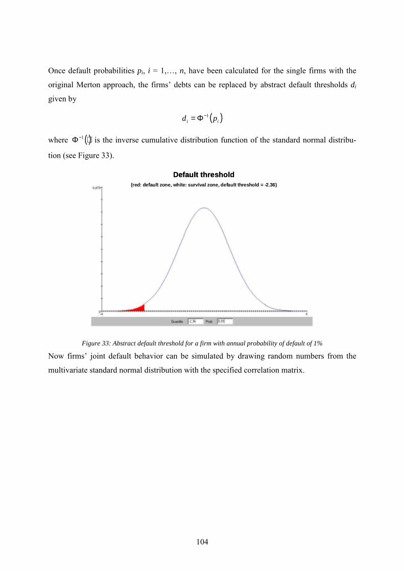
104

Once default probabilities pi, i = 1,…, n, have been calculated for the single firms with the

original Merton approach, the firms’ debts can be replaced by abstract default thresholds di

given by

( )ii pd 1−Φ=

where ( )⋅Φ−1 is the inverse cumulative distribution function of the standard normal distribu-

tion (see Figure 33).

Default threshold(red: default zone, white: survival zone, default threshold = -2.36)

Default threshold(red: default zone, white: survival zone, default threshold = -2.36)

Figure 33: Abstract default threshold for a firm with annual probability of default of 1%

Now firms’ joint default behavior can be simulated by drawing random numbers from the

multivariate standard normal distribution with the specified correlation matrix.

105

Firm 1 Firm 1 Firm 2

Firm

2


Firm

2

Bivariate normal distribution

Simulation results Simulated marginal distributions

ρ = 0

ρ = 0.75

default threshold


Firm

2


Firm

2



ρ = 0

ρ = 0.75


Firm

2


Firm

2




Firm

2


Firm

2


Firm

2


Firm

2



ρ = 0

ρ = 0.75

default threshold

Figure 34: Simulated bivariate normal distributions and marginals

Figure 34 illustrates that firms’ marginal204 asset return distributions always remain un-

changed independent of their correlation. Their joint distribution, however, is distinctly

shaped by the correlation coefficient ρ. Note that firms’ joint default probability, i.e. the prob-

ability that both firms’ sampled asset returns are inferior to the respective default thresholds,

increases sharply with their correlation.

The remaining task is to estimate the asset return correlation matrix. Theoretically, the estima-

tion can be performed based on historical data on firms’ asset value processes using standard

techniques from time-series analysis. In practice, this is much more difficult, though, because

realistic portfolios contain contracts with thousands of clients while the number of correlation

coefficients to be estimated increases quadratically with the number of clients205. For this rea-

son, KMV defines characteristic systematic risk factors for countries and industry sectors.

Each individual firm’s asset return process is regressed against the factor return processes.

Asset return correlations result in turn from regression parameters and factor return correla-

tions206.

204 Note that the marginal distributions do not represent firms’ exact asset value distributions at time t = 1, but rather an

analogous and stochastically equivalent distribution. While keeping the concept of linear correlations between mar-ginal distributions, later generalizations of the KMV-model, such as Credit Metrics or the CRE model, intentionally move away from the concrete interpretation of the distributions as asset value processes.

205 Having n clients, ( )12/ −⋅ nn correlation coefficients are to be estimated. 206 Confer to Lipponer 2000, p. 48f., for details.

106

b) Credit Metrics

A variation of the KMV approach was suggested by Gupton, Finger, and Bhatia in the model

known as Credit Metrics. In Credit Metrics the Vasicek-Kealhofer portfolio model is sepa-

rated from Merton’s option pricing method to calculate default probabilities. Default and also

transition probabilities from one grade to the other are considered as being exogenously given

through company ratings so that the firms’ asset value processes are no longer relevant to fit

the model. This enlarges the applicability of the model from public to all externally or inter-

nally rated companies.

The concept of dependence between counterparties in Credit Metrics is identical to the KMV

approach. The interpretation of the multivariate normal and the marginal distributions as

firms’ joint and marginal asset return distributions is now purely intuitive in the Credit Met-

rics context, so that it would be more correct to rather speak of abstract risk index distribu-

tions. Their main role in the model is to extend the individual firms’ transition probabilities as

given by their ratings to joint transition probabilities for the entire portfolio of firms.

All other changes in Credit Metrics with regard to the KMV portfolio model are technical in

nature and motivated by the lack of actual asset value data. This concerns especially the cal-

culation of correlations between companies’ risk indices since the regression of asset value

processes against systematic factor processes is no longer possible. For public companies

Gupton et al. propose the consideration of equity prices as a proxy for asset values and to use

them to define systematic risk factors for industry sectors and countries207.

Individual firms are mapped to systematic risk factors by their representation in the respective

sectors and countries. Gupton et al. do not tackle the question how a company’s representa-

tion in a certain environment can be measured. However, this gap can be filled by using a

firm’s turnover or profit in a certain market relative to its total turnover or profit as an indica-

tor for its representation in that market.

To avoid the problem that two identical firms are entirely correlated so that they either both

default at once or do not default at all, Gupton et al. introduce the concept of idiosyncratic

risk. A company’s idiosyncratic risk, as being opposed to its systematic risk, signifies the per-

centage of the variance of its risk index that cannot be explained by systematic factors. Gup-

ton et al. do not state how systematic and idiosyncratic risk components can be estimated. For

public companies, however, systematic risk is given as the R2 of the regression of the firms

207 Gupton et al. 1997, p. 92ff.

107

equity returns against the returns of its systematic risk factor. Idiosyncratic risk now can be

calculated as 1 - R2.208

It is a slight imperfection in Credit Metrics that Gupton et al. extend on the one hand the Va-

sicek-Kealhofer model to non-public companies by the use of rating data for default

probabilities, but on the other hand do not provide a means to estimate the risk index

correlations of this type of company. In this version, Credit Metrics does effectively not go

beyond the Vasicek-Kealhofer model.

This problem can be solved if systematic risk factors are chosen that do not involve equity

prices. We suggest the gross value added as a suitable indicator for systematic risk since it has

a number of major advantages:

• It has been calculated by statistical bureaus in all economically important countries for

all relevant industry sectors for many years so that relatively long time series are pub-

licly available.

• It can be calculated for individual companies by subtraction of purchases from turn-

over.

• It is a more basic and stable indicator for economic performance than equity price in-

dices because it is not superimposed by speculative influences.

c) Homogenous Portfolios

For general portfolios the normal correlation model can only be solved to get the portfolio

loss distribution using simulation techniques. For the special case of infinitely large homoge-

nous portfolios an analytic solution exists and the loss distribution is given as a parametric

function.

A homogenous portfolio is defined as consisting only of identical clients in terms of

probabilities of default p, exposure E, risk index correlations209 ρ , and expected loss given

default λ210. Without loss of generality, we assume that all risk index distributions are

208 Note that Gupton et al. define a firm’s systematic risk as the part of the standard deviation of its risk index that is ex-plained by systematic risk factors (p. 100). Though being equivalent to the definition we stated above – it is just the square root of our definition -, it has the drawback that in this setting systematic and idiosyncratic risk usually sum to more than 100%.

209 Risk index correlations ρ have to be non-negative because otherwise the sum of risk indices would have a negative variance v since v is given as

( )12/ −⋅⋅+= nnnv ρ

where n is the number of clients in the portfolio. Thus, for negative ρ the maximum number of clients in a homogenous portfolio is

108

λ210. Without loss of generality, we assume that all risk index distributions are centered and

have variance 1.

Each client’s risk index Xi is then given as

ii ZYX ⋅−+⋅= ρρ 1

with ni ,...,1= if n is the number of clients in the portfolio where Y and Zi are standard nor-

mally distributed.

We can now state

Theorem 2211: In a homogenous portfolio containing n clients each having an exposure of E = 1/n and risk

index correlations 10 <≤ ρ the α-percentile212 of the asymptotic portfolio loss distribution is

given as

( )( ) ( ) ( ) ( )

−−Φ⋅−Φ

Φ⋅==−−

∞→ ραρ

λλραλρα1

1,,;,,,;lim

11 ppLnEpL

n.

Proof: By definition of the model, client i defaults if

( )( )

ρρ

ρρ

−⋅−Φ

≤⇔

Φ≤⋅−+⋅=−

−

1

11

1

YpZ

pZYX

i

ii

for ni ,...,1= .

Hence, client i’s probability of default conditional to Y is given as

−

=ρ

ρ 2n

where x denotes the integer part of x. Since we are interested in asymptotic results for ∞→n , we will only con-

sider non-negative correlations 0≥ρ . 210 Note that we do not assume recovery rates or loss given default rates as being fixed. They may be random with the

same mean (not necessarily the same distribution) being independent from all other random variables in the model such as systematic and idiosyncratic risk factors.

211 A similar version of Theorem 2 was probably first proved by Vasicek 1991. For other proofs or proof concepts see Gersbach / Wehrspohn 2001, Overbeck / Stahl 1999, Finger 1998.

212 The α-percentile of the portfolio loss distribution is defined as

( ) ( ) αα ≥≤= lPlL loss:inf .

( )αL is also called the portfolio value at risk at confidence level α.

109

( )

−⋅−Φ

Φ=−

ρρ

1|defaultsclient

1 YpYiP

because iZ is standard normally distributed for ni ,...,1= .

Moreover, since the idiosyncratic components iZ of clients’ risk indices are stochastically

independent, it follows from the law of large numbers that the percentage of clients defaulting

in the portfolio given Y is equal to their conditional probability of default almost surely213 if

∞→n .

Note that asymptotically the number of defaulting clients goes to infinity as well if the condi-

tional probability is positive. Thus, again by the law of large numbers, the portfolio loss con-

ditional to Y is equal to

( )

−⋅−Φ

Φ⋅=−

ρρ

λ1

|Loss1 Yp

Y

since the individual loss given default rates are stochastically independent and limited with

the same mean λ.

The inverse cumulative loss distribution function can immediately be derived from this ex-

pression for portfolio losses because the systematic risk factor Y is the only remaining random

component in portfolio losses and the conditional portfolio loss given Y is monotonously de-

creasing in Y. The α-percentile of the portfolio loss distribution, therefore, maps one-to-one to

the (1 – α)-percentile of the distribution of Y. The (1 – α)-percentile of Y is given by

( )α−Φ− 11 because Y is standard normally distributed. This completes the proof.

A few special cases are of interest:

• For ρ = 0, we have

( ) ( )( ) pppL ⋅=ΦΦ⋅= − λλλα 1,0,; ,

i.e. the portfolio loss distribution is constant at the expected loss as a direct consequence

of the law of large numbers. This is due to the fact that in the normal correlation model

uncorrelated risk indices are automatically independent. This is a very special feature of

213 I.e. with probability 1.

110

the normal distribution, though, that does not carry over to the more general case that we

will discuss in the next section.

• For ρ > 0, we have

( ) λλραα

=→

,,;lim1

pL ,

i.e. for any positive dependencies in the model, the loss distribution converges in the con-

fidence level α towards the loss of the entire portfolio.

• For 1→ρ the loss distribution converges towards the discontinuous step function l given

by

−≤

=else,

1if,0λ

α pl .

Figure 35 illustrates the loss distributions of homogenous portfolios for various correlations

and a default probability of 0.5%. Again, it is obvious that the degree of dependence between

clients, i.e. the size of correlations in this model, very strongly influences portfolio risk, espe-

cially for high confidence levels α.

Loss distributions of homogenous portfolios in the normal correlation model

(λ = 1, p = 0.5%)

0%

10%

20%

30%

40%

50%

60%

70%

80%

90%

100%

0,00010,0010,010,11

Confidence level α

Loss

in p

erce

nt o

f por

tfolio

exp

osur

e

ρ = 0 ρ = 0.1 ρ = 0.2 ρ = 0.3 ρ = 0.4 ρ = 0.5ρ = 0.6 ρ = 0.7 ρ = 0.8 ρ = 0.9 ρ = 0.99 ρ = 0.999

0 0.9 0.99 0.999 0.9999

α = 99.5%

Figure 35: Loss distributions of homogenous portfolios in the normal correlation model 1

We express another interesting feature of homogenous portfolios as

Theorem 3:

Assume a homogenous portfolio as in Theorem 2. Let 21 ρρ < . Then there exists a confidence

level *α such that

111

( ) ( )( ) ( )( ) ( ) *

12

*12

*12

if,,;,,; if,,;,,; if,,;,,;

ααλραλραααλραλραααλραλρα

>>==<<

pLpLpLpLpLpL

Theorem 3 states that increasing correlations and, thus, increasing dependencies and concen-

trations in the portfolio imply lower portfolio risk for low confidence levels α and higher

portfolio risk for high confidence levels in terms of the respective percentiles of the loss dis-

tribution214. In other words, high correlations reduce portfolio risk most of the time, but also

increase the probability of extreme losses.

Proof:

Since ( )⋅Φ is monotonously increasing, the statement ( ) ( )λραλρα ,,;,,; 12 pLpL>=<

is equivalent to

( ) ( ) ( ) ( ) ( ) ( )11

11

1

2

12

1

2 ;1

11

1:; ρα

ραρ

ραρ

ρα Fpp

F =−

−Φ⋅−Φ

>=<

−−Φ⋅−Φ

=−−−−

with ( ) ( )12 ;; ραρα FF = if and only if

( ) ( ) ( )1;011

111:

2112

112* ∈

⋅−−⋅−Φ⋅−−−

Φ−==−

ρρρρρρ

ααp

.

The theorem then follows from215

( ) ( )( ) ( )( ) ( )1*

*11

1*1

2

22

* ;11

111

1; ρα

αϕρρ

αϕρρ

ρα FF ′=−Φ

⋅−

>−Φ

⋅−

=′−−

because ( )ρα ;F is continuous in α for all 10 <≤ ρ .

In other words, ( )1;ραF and ( )2;ραF intersect only in 0=α , 1=α and *αα = and for the

slope we have ( ) ( )1*

2* ;; ραρα FF ′>′ in *α , which implies that ( ) ( )12 ;; ραρα FF < for

214 See above footnote 212. 215 Here ( )⋅ϕ is the standard normal density function. It was used that for a continuous invertible function

yxYXf v,: → we have ( )( ) ( )( )yffyf

11 1

−−

′=

′.

112

*αα < and ( ) ( )12 ;; ραρα FF > for *αα > . The theorem then follows from the monotonicity

of ( )⋅Φ .

Note that *α is increasing in 1ρ and 2ρ and that

( ) ( ) p−===→→

1,lim,lim 21*

121*

1

*

21max ρραρραα

ρρ.

Figure 36 gives a visual example of Theorem 3 and its implications.

Loss distributions of homogenous portfolios in the normal correlation model

(λ = 1, p = 0.5%)

0,001

0,01

0,1

1

0,00010,0010,010,11

Confidence level α

Loss

rela

tive

to p

ortfo

lio e

xpos

ure

ρ = 0 ρ = 0.1 ρ = 0.2 ρ = 0.3 ρ = 0.4 ρ = 0.5ρ = 0.6 ρ = 0.7 ρ = 0.8 ρ = 0.9 ρ = 0.99 ρ = 0.999

0 0.9 0.99 0.999 0.9999

α = 99.5%

Figure 36: Loss distributions of homogenous portfolios in the normal correlation model 2

2. The generalized correlation model (CRE model)

While being economically intuitive, a major drawback of the normal correlation model is the

somewhat arbitrary choice of the multivariate normal distribution to describe the joint move-

ments of clients’ individual risk indices. Historical reasons certainly were dominant in this

selection because normal distributions appear as finite dimensional marginal distributions of

the log-returns of the geometric Brownian motion, the standard model of continuous stochas-

tic processes. This is used for example in the classic Black-Scholes-Merton model and is also

by far the best understood continuous multivariate distribution.

In the present discussion, however, a typical criticism of the normal distribution is that it is

not well adapted to the specific features of much financial data. This assessment refers espe-

cially to the phenomenon that many empirical distributions have long tails, i.e. that large de-

113

viations from the mean of a distribution are observed much more frequently than one would

expect if the underlying distribution were normal.

1

10

100

1000

-0.04 -0.02 0 0.02 0.04

Häuf

igkeit

Logarithmische Returns DAX

Freq

uenc

y

A long tail distribution in finance: daily DAX-returns

DAX-returns (logarithmic)

blue: normal distribution red: normal inverse gauss distribution

1

10

100

1000

-0.04 -0.02 0 0.02 0.04

Häuf

igkeit

Logarithmische Returns DAX

Freq

uenc

y

A long tail distribution in finance: daily DAX-returns

DAX-returns (logarithmic)

blue: normal distribution red: normal inverse gauss distribution

Figure 37: An empirical long tail distribution in finance: DAX-returns

Figure 37 gives an example of the normal and a long tail distribution fitted to the same finan-

cial data, daily DAX-returns from January 1, 1991 to November 30, 2000. It is apparent that

the long tail distribution216 is much better adapted to the frequency of extreme returns than the

normal distribution while both distributions are quite similar in the region of small deviations

from the mean.

In the normal correlation model, two things were fundamental: the marginal distributions that

were needed to calculate clients’ default and transition thresholds and the correlation matrix

of clients’ risks indices. In order to extend the model, note that a multivariate distribution is in

general not uniquely determined by its marginal distributions and its correlation structure.

However, exceptions in that respect are spherical and elliptical distributions.

A distribution D is called spherical217 if it is invariant under orthogonal transformations, i.e. if

for a random vector nX R∈ with DX ~ and any orthogonal map nnU ×∈ R the equation

( ) ( )UXX L=L

holds218. If D has a density d than this definition is equivalent to saying that d is constant on

spheres.219

216 We chose the normal inverse gauss distribution in the example, a family of distributions where the length of the tails

can be continuously adapted due to a further parameter besides mean and covariance matrix. See below for details. 217 Or ‘spherically symmetric’.

114

Let S be the family of all spherical distributions. A distribution D is called elliptical220 if it is

an affine linear transformation of a spherical distribution221, i.e. if for a random vector nX R∈ with DX ~ and a random vector nY R∈ with ( ) S∈YL there exists nR∈µ and

nnA ×∈ R such that

YAX ⋅+= µ .

The best known example of spherical or elliptical distributions, respectively, is the family of

multivariate normal distributions so prominent in the normal correlation model. Figure 38

shows plots of densities and their contours of the bivariate normal distribution for correlations

0=ρ (the spherical case) and for %75=ρ (an elliptical case).

The bivariate normal distribution

Contours

Densitiesρρρρ = 0 ρρρρ = 75%

Spherical and elliptical distributionsThe bivariate normal distribution

Contours

Densitiesρρρρ = 0 ρρρρ = 75%

Spherical and elliptical distributions

Figure 38: Spherical and elliptical distributions

218 ( )XL denotes the law of X. The expression denotes that the distributions of X and of UX are equal. 219 Fang et al. 1989, definition 2.1., p. 29. 220 Or ‘elliptically symmetric’. 221 Fang et al. 1989, definition 2.2., p. 31.

115

Elliptical distributions are an interesting generalization of the normal distribution in the corre-

lation model because a multivariate elliptical distribution is uniquely determined by its uni-

variate marginals, its mean and its covariance matrix since the type of all marginals is the

same222.

Not all symmetric univariate distributions are possible as marginal distributions of an ellipti-

cal distribution in nR for any N∈n . It can be shown, however, that a univariate distribution

D is the marginal distribution of a spherical distribution in nR for any N∈n if and only if it

is a variance mixture of centered normals223. Hence224, D can be defined by its density func-

tion

( )sdWs

xs

xf ∫∞

−=

0

2

2exp1

21)(π

where the weight or mixing distribution W only takes values on ),0( ∞ , i.e. a variance mixture

of normals is a normal distribution with random variance. This definition immediately implies

that a random variable DX ~ can be written as

YwX ⋅=

where Y is standard normally distributed, Ww ~ , and Y and w are stochastically independent.

Example 1

A well known example of a normal variance mixture is the Student-t distribution with n de-

grees of freedom. Here the mixing distribution w is given as

ϑnw =

where 2~ nχϑ .

Example 2

A more flexible family of mixture distributions is the generalized hyperbolic distribution. The

one-dimensional centered and symmetric version of the generalized hyperbolic distribution

has three free parameters λ, α, δ and is defined by its Lebesgue-density

( ) ( ) ( )( ) ( )222/1

2/2/12,,a,,; xxxgh +−⋅= −− δαδδαλδαλ λλ K

222 Cf. Embrechts et al. 1999, p. 11. 223 Fang et. al, 1989, theorem 2.21, p. 48. Note that there exist univariate distributions that are no variance mixtures of

normals that can be marginals of spherical distributions for some, but not all N∈n . 224 Note that any mixture of normals has a density with respect to Lebesgue measure.

116

with

( )( )δλδπ

αδαλλ

λ K⋅⋅=

2,,a

2/1

where ( )⋅λK is a modified Bessel function of the third kind with index λ and R∈x . Alterna-

tively, the generalized hyperbolic distribution can be defined by its mixing distribution. This

is the generalized inverse Gauss distribution with density

( ) ( )( )

+−⋅= − xx

xxgig ψχψχχψχψ λ

λ

λ

21exp/,; 1

2/

K

for 0>x and 2δχ = and 2αψ = .

The generalized hyperbolic distribution is continuous in its parameters and has the normal and

the t-distribution as limiting cases:

For ∞→δα , , 2σαδ → and any given λ, the generalized hyperbolic distribution converges

towards ( )2,0 σN .225

On the other hand, for 0=α , νδ = and 2/νλ −= it is equal to the t-distribution with ν

degrees of freedom.226

Example 3

An interesting special case of the generalized hyperbolic distribution is the normal inverse

Gauss distribution (NIG). It is obtained for 2/1−=λ and has the inverse Gauss distribution

( )

+

+−⋅⋅⋅

= ψχψχπχχψ x

xxxig

21exp

2,; 3

as mixing distribution.

The NIG is particularly interesting as an alternative for the normal distribution in the correla-

tion model because it is not only infinitely divisible227, but also closed under convolution.

Hence, similar to the normal distribution, it generates a Lévy-motion whose finite dimen-

sional marginals are all NIG-distributed228. Therefore, the intuitive interpretation in the Va-

225 Cf. Prause 1999, p. 3. 226 Cf. Prause 1999, p. 5. 227 As is any generalized hyperbolic distribution. Cf. Barndorff-Nielsen and Halgreen 1977. 228 Cf. Eberlein et al. 1998, p. 6f., who use the Lévy-motion generated by the NIG instead of the classical geometric

Brownian motion to model financial price processes.

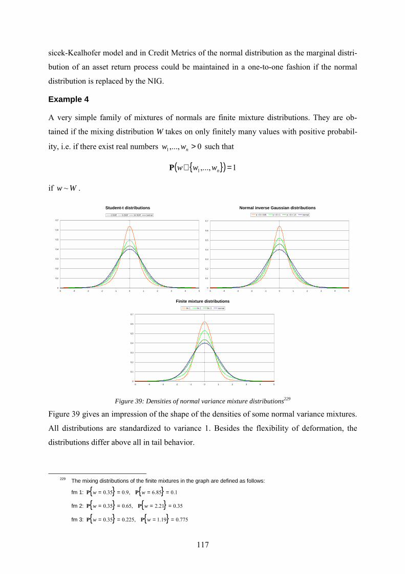
117

sicek-Kealhofer model and in Credit Metrics of the normal distribution as the marginal distri-

bution of an asset return process could be maintained in a one-to-one fashion if the normal

distribution is replaced by the NIG.

Example 4

A very simple family of mixtures of normals are finite mixture distributions. They are ob-

tained if the mixing distribution W takes on only finitely many values with positive probabil-

ity, i.e. if there exist real numbers 0,...,1 >nww such that

( ) 1,...,1 =∈ nwwwP

if Ww ~ .

Student-t distributions

0

0,1

0,2

0,3

0,4

0,5

0,6

0,7

-5 -4 -3 -2 -1 0 1 2 3 4 5

3 DOF 5 DOF 10 DOF normal

Normal inverse Gaussian distributions

0

0,1

0,2

0,3

0,4

0,5

0,6

0,7

-5 -4 -3 -2 -1 0 1 2 3 4 5

α = δ = 0,65 α = δ = 1 α = δ = 1,5 normal

Finite mixture distributions

0

0,1

0,2

0,3

0,4

0,5

0,6

0,7

-5 -4 -3 -2 -1 0 1 2 3 4 5

fm 1 fm 2 fm 3 normal

Figure 39: Densities of normal variance mixture distributions229

Figure 39 gives an impression of the shape of the densities of some normal variance mixtures.

All distributions are standardized to variance 1. Besides the flexibility of deformation, the

distributions differ above all in tail behavior.

229 The mixing distributions of the finite mixtures in the graph are defined as follows:

fm 1: 1.085.6,9.035.0 ==== ww PP

fm 2: 35.021.2,65.035.0 ==== ww PP

fm 3: 775.019.1,225.035.0 ==== ww PP

118

Tail behavior of normal mixture distributions

-18

-16

-14

-12

-10

-8

-6

-4

-2

0

-8 -6 -4 -2 0 2 4 6 8

log-

dens

ity

finite mixture NIG: a = d = 0,661 t: 3 DOF normal

Figure 40: Tail behavior of normal mixture distributions

Figure 40 shows that NIG and t-distributions have exponentially decreasing tails while tails of

finite mixture distributions and the normal distribution decrease of order230 ( )2xeO − .

However, interpreting the illustration above, we can prove the following

Theorem 4 and definition:

Let f be the density function of a distribution F with expectation µ and variance 2σ . We say

that F has long tails compared to the normal distribution if and only if

( )( ) 1lim

2,

>∞→ x

xfx

σµϕ

where 2,σµϕ is the density of the normal distribution with expectation µ and variance 2σ .

Let D be a normal variance mixture with non-degenerate mixing distribution. Then D has

long tails compared to the normal distribution.

Proof:

Without loss of generality, we can assume that .1and0 2 == σµ Let W be the mixing distri-

bution of D and Ww ~ . Then there exists an s > 1 such that 0: >≥= swp P .

Let f be the density of D. Then we have

230 A function f is of order ( )( )xgO if and only if

( )( ) 0lim ≠=

∞→

cxg

xf

x, i.e. ( )⋅O describes the asymptotic expansion of f.

119

( )( ) ( ) ∞==

⋅

⋅=

⋅⋅>

−

∞→−

−

∞→∞→∞→

sx

xx

sx

xxxe

sp

es

epx

sx

sp

xxf 11

2

2

22

2

2

limlim

1

limlimϕ

ϕ

ϕ.

We say that a model defines a representation of the generalized correlation model, if its risk

index distribution is a variance mixture of normals. According to the choice of the risk index

distribution in the generalized correlation model, we will also speak of the Student-t-

correlation model, the finite mixture correlation model etc. The normal correlation model is

just a special case in this framework. It is obtained for cw ≡ for some constant c > 0.

To better understand the impact of the choice of clients’ risk index distributions on the result-

ing portfolio risk, we look at

a) Homogenous Portfolios

because we can derive analytic loss distributions for this special class of portfolios making it

particularly convenient to compare the results.

As in the normal correlation model, we define a homogenous portfolio as consisting only of

identical clients in terms of probabilities of default p, exposure E, risk index correlations231

ρ , and expected loss given default λ232. Without loss of generality, we may assume that all

risk index distributions are centered and have variance 1.

Let D be the distribution of risk indices. We assume that D is a mixture of normals with mix-

ing distribution W, such that

DXw ~⋅

if

( )1,0~and~ NXWw .

In the generalized correlation model, in a homogenous portfolio each client’s risk index Xi is

then given as

( )ii ZYwX ⋅−+⋅⋅= ρρ 1

231 See above footnote 209. 232 Again we do not assume recovery rates or loss given default rates as being fixed. They may be random with the same

mean (not necessarily the same distribution) being independent from all other random variables in the model such as systematic and idiosyncratic risk factors.

120

with ni ,...,1= if n is the number of clients in the portfolio where Y and Zi are standard nor-

mally distributed.

To facilitate the exposition of the results,

• let F be the cumulative distribution function of D,

• let Φ be the cumulative distribution function of the standard normal distribution,

• let L be the loss distribution of the portfolio under consideration, i.e. the cumulative dis-

tribution function of portfolio losses.

We begin with the derivation of the portfolio loss distribution of homogenous portfolios in the

generalized correlation model, then calculate the density of the portfolio loss distribution and

compare the results for the normal and generalized correlation model. Finally, we show how

the approach can be extended to more complex forms of homogenous portfolios.

(1) Portfolio loss distribution

Theorem 5: In the generalized correlation model, in a homogenous portfolio containing n clients each hav-

ing an exposure of E = 1/n and risk index correlations 10 << ρ the asymptotic portfolio loss

distribution is given as

( ) ( )( )

( ) ( )

⋅Φ⋅−⋅−

Φ−=

≤==

−−

∞→

ρλρ

λρλρ

wlwpF

lnEplLplL

w

n

/11

Loss,,,;lim,,;

11

E

P

where ( )⋅wE is the expectation functional with respect to w.

Proof: The first part of the proof is similar to the proof of Theorem 2.

By definition of the model, client i defaults if

( ) ( )( )

ρρ

ρρ

−⋅⋅⋅−

≤⇔

≤⋅−+⋅⋅=−

−

1

11

1

wYwpF

Z

pFZYwX

i

ii

for ni ,...,1= .

Hence, client i’s probability of default conditional to w and Y is given as

121

( )

−⋅⋅⋅−

Φ=−

ρρ

1,|defaultsclient

1

wYwpF

YwiP




in the portfolio given w and Y is equal to their conditional probability of default with probabil-

ity one if ∞→n .

Note that asymptotically the number of defaulting clients goes to infinity as well if the condi-

tional probability is positive. Thus, again by the law of large numbers, the portfolio loss con-

ditional to w and Y is equal to

( )

−⋅⋅⋅−

Φ⋅=−

ρρ

λ1

,|Loss1

wYwpF

Yw

since the individual loss given default rates are stochastically independent and limited with

the same mean λ.

The unconditional portfolio loss distribution is, therefore, given as

( )

( ) ( )

( ) ( )

( ) ( )

( ) ( )

( ) ( )

⋅Φ⋅−⋅−

Φ−=

⋅Φ⋅−⋅−

≤−=

⋅Φ⋅−⋅−

≤−=

⋅Φ⋅−⋅−

≥=

Φ≤−⋅

⋅⋅−=

≤

−⋅⋅⋅−

Φ⋅=≤

−−

−−

−−

−−

−−

−

ρλρ

ρλρ

ρλρ

ρλρ

λρ

ρ

ρρλ

wlwpF

ww

lwpFY

wlwpF

Y

wlwpF

Y

lw

YwpF

lw

YwpFl

w

w

/11

|/1

1

/11

/1

/1

1Loss

11

11

11

11

11

1

E

PE

P

P

P

PP

122

The portfolio loss distribution is particularly easy to calculate for finite mixture distributions

because in this case the expectation functional ( )⋅wE is reduced to a simple sum. Let the mix-

ing distribution W be a probability distribution on kww ,...,1 with ii pww ==P for

ki ,...,1= . Then the portfolio loss distribution can be written as

( ) ( ) ( )∑

=

−−

⋅Φ⋅−⋅−

Φ⋅−=k

i i

ii w

lwpFpplL

1

11 /11,,;

ρλρ

λρ .

Portfolio loss distributions(ρρρρ = 20%, p = 0.5%, λλλλ = 100%)

0%

10%

20%

30%

40%

50%

60%

70%

80%

90%

100%

1E-100,0000000010,000000010,00000010,0000010,000010,00010,0010,010,11Confidence level

Loss

in p

erce

nt o

f por

tfolio

exp

osur

e


0 1 - 1E-101 - 1E-90.999999990.99999990.9999990.999990.99990.9990.990.9

Figure 41: Portfolio loss distributions in the generalized correlation model based on finite mixture distributions

Figure 41 shows the loss distributions for a homogenous portfolio resulting from the finite

mixture distributions in Figure 39. Note that the loss distributions in the generalized correla-

tion model dominate the loss distribution in the normal correlation model at high confidence

levels, in the example at confidence levels above 92.5% (fm 1), 84.8% (fm 2), and 79.9% (fm

3). We will prove this as a general result in Theorem 9 below.

For more complex mixing distributions the portfolio loss distribution can be calculated using

numerical techniques or Monte Carlo integration.

123

Portfolio loss distributions NIG with shape parameter δδδδ

====

αααα

(correlations = 20%, default probabilities = 0.5%)

0%

10%

20%

30%

40%

50%

60%

0,00010,0010,010,11

Confidence level

Loss

in p

erce

nt o

f por

tfolio

exp

osur

eδ = 10 δ = 8 δ = 6 δ = 4 δ = 2 δ = 1 δ = 0.8 δ = 0.5

0 0.99990.9990.990.9

Figure 42: Portfolio loss distributions in the generalized correlation model based on normal inverse Gaussian distributions

It is a very important feature of the generalized correlation model that clients with uncorre-

lated risk indices are still dependent in their default behavior. We state this fact as


ing an exposure of E = 1/n and risk index correlations 0=ρ , the asymptotic portfolio loss

distribution is given as

( )

( )( )

( )( )

=≤=>

>

Φ≤−

<

Φ≤

= −

−

−

−

2/and2/1if2/and2/1if

2/if

10

/1

2/if/

,0,; 1

1

1

1

λλ

λλ

λλ

λ

lplp

llpFw

ll

pFw

plL P

P

Proof: If risk indices are uncorrelated, client i defaults if

( )( )w

pFZ

pFZwX

i

ii1

1

−

−

≤⇔

≤⋅=.

Along the same lines as in Theorem 5 one can show that the portfolio loss distribution is then

given as

124

( )

( ) ( )

( ) ( ) λ

λ

λ

/

/

Loss

11

11

1

lwpF

lw

pF

lw

pFl

−−

−−

−

Φ⋅≤=

Φ≤=

≤

Φ⋅=≤

P

P

PP

which is equivalent to the formulation in the theorem since ( ) 0/1 <Φ− λl if 2/λ<l ,

( ) 0/1 >Φ− λl if 2/λ>l , and ( ) 0/1 =Φ− λl if 2/λ=l .

Theorem 6 states that – other than in the normal correlation model233 where 0=ρ implies

1Loss =⋅= λpP – uncorrelated risk indices imply in the generalized correlation model a

constant portfolio loss distribution only for p = ½.

For default probabilities p < ½ the loss distribution is not constant, but only takes values be-

tween 0 and λ/2. On the other hand, for default probabilities p > ½ the loss distribution is not

constant either, and only takes values between λ/2 and λ.

2 degrees of freedom

0%

10%

20%

30%

40%

50%

60%

70%

80%

90%

100%

0,000010,00010,0010,010,11Confidence level

Loss

in p

erce

nt o

f por

tfolio

exp

osur

e

p = 0,01 p = 0,1 p = 0,4 p = 0,5 p = 0,6 p = 0,7

0 0.999990.9990.990.9 0.9999


0%

10%

20%

30%

40%

50%

60%

70%

80%

90%

100%


Loss

in p

erce

nt o

f por

tfolio

exp

osur

e

p = 0,01 p = 0,1 p = 0,4 p = 0,5 p = 0,6 p = 0,7

0 0.999990.9990.990.9 0.9999


0%

10%

20%

30%

40%

50%

60%

70%

80%

90%

100%


Loss

in p

erce

nt o

f por

tfolio

exp

osur

e

p = 0,01 p = 0,1 p = 0,4 p = 0,5 p = 0,6 p = 0,7

0 0.999990.9990.990.9 0.9999


0%

10%

20%

30%

40%

50%

60%

70%

80%

90%

100%


Loss

in p

erce

nt o

f por

tfolio

exp

osur

e

p = 0,01 p = 0,1 p = 0,4 p = 0,5 p = 0,6 p = 0,7

0 0.999990.9990.990.9 0.9999

Figure 43: Loss distributions resulting from uncorrelated Student-t-distributed risk indices234

Figure 43 shows that loss distributions remain above or below λ/2 for the respective prob-

abilities of default. If the number of the degrees of freedom of the Student-t-distribution tends

233 The result for the normal correlation model follows from the theorem for 1≡w . In this case Φ=F . 234 The loss given default rate λ is set to 100%.

125

to infinity, i.e. if the t-distributed risk indices converge towards normally distributed risk indi-

ces, the portfolio loss distributions become more and more flat and converge towards

( ) λλ ⋅≡ pplL ,0,; as we would expect from Theorem 6.

If the mixing distribution of the risk index distributions is discrete, as is the case at finite mix-

tures of normals, then the resulting portfolio loss distribution is also discrete if risk index cor-

relations are zero (Figure 44). However, if the mixing distribution converges to a constant, the

loss distribution again converges towards ( ) λλ ⋅≡ pplL ,0,; .

Pw = 0.1 = 0.7, Pw = 3.1 = 0.3

0%

10%

20%

30%

40%

50%

60%

70%

80%

90%

100%

0% 10% 20% 30% 40% 50% 60% 70% 80% 90% 100%

Confidence level

Loss

in p

erce

nt o

f por

tfolio

exp

osur

e

p = 0,01 p = 0,1 p = 0,4 p = 0,501 p = 0,6 p = 0,7

Pw = 0.3 = 0.7, Pw = 2.63 = 0.3

0%

10%

20%

30%

40%

50%

60%

70%

80%

90%

100%

0% 10% 20% 30% 40% 50% 60% 70% 80% 90% 100%

Confidence level

Loss

in p

erce

nt o

f por

tfolio

exp

osur

e

p = 0,01 p = 0,1 p = 0,4 p = 0,501 p = 0,6 p = 0,7

Pw = 0.7 = 0.7, Pw = 1.7 = 0.3

0%

10%

20%

30%

40%

50%

60%

70%

80%

90%

100%

0% 10% 20% 30% 40% 50% 60% 70% 80% 90% 100%

Confidence level

Loss

in p

erce

nt o

f por

tfolio

exp

osur

e

p = 0,01 p = 0,1 p = 0,4 p = 0,501 p = 0,6 p = 0,7

Pw = 0.95 = 0.7, Pw = 1.12 = 0.3

0%

10%

20%

30%

40%

50%

60%

70%

80%

90%

100%

0% 10% 20% 30% 40% 50% 60% 70% 80% 90% 100%

Confidence level

Loss

in p

erce

nt o

f por

tfolio

exp

osur

e

p = 0,01 p = 0,1 p = 0,4 p = 0,501 p = 0,6 p = 0,7

Figure 44: Loss distributions resulting from uncorrelated finite mixture distributed risk indices235

In the remaining case of perfect risk index correlations 1=ρ the differences between the

models disappear. Here clients’ risk indices are given as

YwXX i ⋅==

so that all clients default simultaneously if

( )pFYwX 1−≤⋅= .

However, since FYw ~⋅ is

235 The mixing distribution is a two-point distribution that is standardized to have expectation 1. The loss given default rate λ is set to 100%.

126

( ) ( ) ppYpFYw =Φ≤=≤⋅ −− 11 PP

independent of F.

(2) Portfolio loss density

In the previous section, we considered the asymptotic portfolio loss distribution of homoge-

nous portfolios for an infinite number of clients in the portfolio. Due to the increasing number

of clients, each single client’s exposure converges to zero relative to the total portfolio expo-

sure. Therefore, homogenous portfolios asymptotically do not contain exposure concentra-

tions on specific clients or exposure point masses. This is a necessary condition for the portfo-

lio loss distribution to have a Lebesgue density.

In the next theorem, we derive the portfolio loss density for risk index correlations 10 << ρ .


ing an exposure of E = 1/n and risk index correlations 10 << ρ , the density dL of the asymp-

totic portfolio loss distribution is given as

( ) ( )( )( ) ( )

⋅Φ⋅−⋅−

⋅Φ

⋅⋅−

=−−

− ρλρ

ϕλϕρλ

ρλρ

wlwpF

lplL wd

/1/

11,,;

11

1 E

where ϕ is the standard normal density.

Proof: The portfolio loss density is defined as the first derivative of the cumulative distribution func-

tion of portfolio losses. Thus, we have

( ) ( )

( ) ( )

( ) ( ) ( ) ( )( )

⋅

Φ⋅

⋅−⋅

⋅−⋅

⋅Φ⋅−⋅−

−=

⋅Φ⋅−⋅−

Φ−=

=

−

−−

−−

λλϕρρ

ρλρ

ϕ

ρλρ

λρλρ

1/

111

/1

/11

,,;,,;

1

11

11

lww

wlwpF

wlwpF

ldd

plLld

dplL

w

w

d

E

E

since the standard normal density is continuous and integrable so that we may derive within

the expectation functional wE .

127

Figure 45 shows loss densities for a model where the risk index distribution is a bi-mixture

defined by its mixing distribution 5.08.1and5.02.0 ==== ww PP for various default

probabilities and risk index correlations.

Risk index correlations = 1%

0

2

4

6

8

10

12

14

16

0% 10% 20% 30% 40% 50% 60%Loss in percent of portfolio exposure

Den

sity

p = 0,2 p = 0,23 p = 0,27 p = 0,3


0

1

2

3

4

5

6

7


Den

sity

p = 0,2 p = 0,23 p = 0,27 p = 0,3


0

1

2

3

4

5

6


Den

sity

p = 0,2 p = 0,23 p = 0,27 p = 0,3


0

1

2

3

4

5

6

7

8

9

10


Den

sity

p = 0,2 p = 0,23 p = 0,27 p = 0,3

Figure 45: Portfolio loss densities in the bimixture correlation model

Note that the density function is not necessarily unimodal. The number of modes varies with

default probabilities, risk index correlations and also with the type of mixing distribution.

We formulate this observation as

Theorem 8: In the generalized correlation model, the number of modes of the asymptotic portfolio loss

distribution of a homogenous portfolio with risk index correlations 10 << ρ , is smaller or

equal to the cardinality of the support of the mixing distribution of the risk index distribution.

Proof: It can be shown by derivation of the portfolio loss density of the normal correlation model236,

that the portfolio loss distribution is unimodal in this model (see also Figure 46). The theorem

then follows immediately from the fact that the portfolio loss distribution in the generalized

correlation model is the convex combination of loss distributions in the normal correlation

model.

236 The portfolio loss density of the normal correlation model is obtained by setting cw ≡ for some constant c in Theorem

8.

128


0

10

20

30

40

50

60

70

80

90

0% 2% 4% 6% 8% 10% 12%

Loss in percent of portfolio exposure

Den

sity

p = 0,02 p = 0,04 p = 0,06 p = 0,08


0

5

10

15

20

25

30

35

40

45

50

0% 2% 4% 6% 8% 10% 12%


Den

sity

p = 0,02 p = 0,04 p = 0,06 p = 0,08


0

10

20

30

40

50

60

0% 2% 4% 6% 8% 10% 12%


Den

sity

p = 0,02 p = 0,04 p = 0,06 p = 0,08


0

50

100

150

200

250

300

0% 2% 4% 6% 8% 10% 12%


Den

sity

p = 0,02 p = 0,04 p = 0,06 p = 0,08

Figure 46: Portfolio loss densities in the normal correlation model

Figure 47 gives an example of trimodal loss densities in the trimixture correlation model.

Portfolio loss densities in the trimixture correlation modelRisk index correlations = 0.1%

0

5

10

15

20

25

30

35

40

0% 5% 10% 15% 20% 25% 30% 35% 40% 45%


Den

sity

p = 0,2 p = 0,23 p = 0,27 p = 0,3

Figure 47: Trimodal portfolio loss densities in the trimixture correlation model237

We saw in the previous section, that the portfolio loss distribution is discrete for zero correla-

tions in the finite mixture correlation model while it is Lebesgue absolutely continuous for

237 The distributions differ only in the clients’ default probability p and share the mixing distribution

3/178.1,3/11,3/12.0 ====== www PPP . The modes of the original loss densities in the convex combi-nations are well visible and well separated.

129

positive risk index correlations. We would, therefore, expect that loss densities degenerate in

this model if risk index correlations go to zero, a phenomenon that is illustrated by Figure 48.

Portfolio loss densitiesRisk index correlations = 0.0001%

0

500

1000

1500

2000

2500

0% 10% 20% 30% 40% 50% 60% 70% 80% 90% 100%


Den

sity

p = 0,05 p = 0,1 p = 0,4 p = 5,01 p = 0,6 p = 0,7

Cumulative portfolio loss distributionsRisk index correlations = 0%

0%

10%

20%

30%

40%

50%

60%

70%

80%

90%

100%

0% 10% 20% 30% 40% 50% 60% 70% 80% 90% 100%

Confidence level

Loss

in p

erce

nt o

f por

tfolio

exp

osur

e

p = 0,05 p = 0,1 p = 0,4 p = 0,501 p = 0,6 p = 0,7

Figure 48: The low correlation effect in the finite mixture model238

For extremely low correlations, the loss density develops peaks at the discontinuity points of

the loss distribution. The relative size of the peaks is approximately equal to the size of the

point masses at the discontinuity points.

(3) Comparison of the normal and the generalized correlation model

So far the replacement of the normal distribution by a general distribution, determined by its

marginal distributions and a correlation structure, was rather intuitively motivated as a general

topic in the correlation model and by the fact that all of these distributions have long tails, a

feature frequently found in finance (see section II.A.2 above). The next theorem gives a fun-

damental reason as to why the choice of the normal distribution as the distribution of risk in-

dices might cause structural problems in the correlation model and why it should be carefully

overthought. The theorem also shows that the analysis of homogenous portfolios can be ex-

tremely helpful in the understanding of the economic and model theoretic consequences of

allegedly natural mathematical assumptions.

Theorem 9:

Let ( )λρ,,;1 pLN ⋅− and ( )λρ,,;1\ pL NG ⋅− be the inverse cumulative distribution functions of the

asymptotic portfolio loss distributions of a homogenous portfolio with risk index correlations

10 << ρ in the generalized correlation model with a normal and a non-normal risk index dis-

tribution, respectively. Then there exists a confidence level *α such that

( ) ( )λραλρα ,,;,,; 11\ pLpL NNG

−− >

238 The actual model displayed in the charts is a bimixture model with mixing distribution

3.04.2and7.04.0 ==== ww PP .

130

for all confidence levels *αα > and 21≠p .

Alternatively: Let ( )λρ,,; pLN ⋅ and ( )λρ,,;\ pL NG ⋅ be the cumulative distribution functions

of the asymptotic portfolio loss distributions of the same homogenous portfolio with risk in-

dex correlations 10 << ρ in the generalized correlation model with a normal and a non-

normal risk index distribution, respectively. Then there exists a portfolio loss *l such that

( ) ( )λρλρ ,,;,,;\ plLplL NNG <

for all portfolio losses *ll > .

Theorem 9 states that for high confidence levels the normal correlation model reports less risk

in any homogenous portfolio than any other correlation model (see Figure 49). I.e. at the high

confidence levels risk managers are interested in, the normal correlation model is not robust

against misspecifications in the risk index distribution.

Normal versus Student-t correlation modeln = degrees of freedom

0,000001

0,00001

0,0001

0,001

0,01

0,1

1

0,00010,0010,010,11Confidence level

Loss

rela

tive

to p

ortfo

lio e

xpos

ure

n = 2 n = 4 n = 6 n = 8 n = 10 n = 30 Normal

0 0.99990.9990.990.9

Normal versus hyperbolic correlation model NIG with shape parameter δδδδ

0,000001

0,00001

0,0001

0,001

0,01

0,1

1

0,0010,010,11Confidence level

Loss

rela

tive

to p

ortfo

lio e

xpos

ure

Normal δ = 10 δ = 8 δ = 6 δ = 4 δ = 2 δ = 1 δ = 0.8 δ = 0.5

0 0.9990.990.9

Normal versus finite mixture correlation model

0%

1%

10%

100%


Loss

rela

tive

to p

ortfo

lio e

xpos

ure


0 0.999990.9990.9990.990.9

Figure 49: Portfolio loss distributions in the normal versus the generalized correlation model

Proof:

Let ( )λρ,,;, pL Nd ⋅ and ( )λρ,,;\, pL NGd ⋅ be the portfolio loss densities in the correlation

model with a normal and a non-normal risk index distribution. We show that a portfolio loss *l exists so that ( ) ( )λρλρ ,,;,,; \,, plLplL NGdNd < for all portfolio losses *ll > (see Figure

131

50). This implies that ( ) ( )λρλρ ,,;,,;\ plLplL NNG < and, thus, the second version of the

theorem because ( ) ( ) λλρλρ == ,,;1,,;1\ pLpL NNG .

Portfolio loss densities in the normal and the generalized correlation model

(p = 0.5%, ρρρρ = 20%, λλλλ = 100%)

-8

-7

-6

-5

-4

-3

-2

-1

0

1

2

0% 2% 4% 6% 8% 10% 12% 14% 16% 18% 20%


log-

dens

ity

finite mixture normal

Figure 50: Portfolio densities in the normal and the generalized correlation model

Theorem 7 implies that

( )( )

( ) ( )

( ) ( )

( ) ( ) ( ) ( )

( )[ ] ( )[ ]

( ) ( ) ( ) ( )

Φ⋅Φ⋅−⋅−⋅Φ⋅−⋅+

−Φ⋅=

Φ⋅−−Φ⋅+

⋅Φ⋅−⋅−

⋅−=

Φ⋅−−Φ

⋅Φ⋅−⋅−

=

=

−−−−

=

−−

−−−−

−−

−−

2

1

:

1111

:

2121

211211

11

11

,

\,

/12/12

21exp

/121/1

21exp

/1

/1

,,;,,;

T

T

W

W

WNd

NGd

plwpFlw

pFpww

lpw

lwpF

lp

wlwpF

plLplL

λρλρ

ρ

ρλρ

ρλρ

ρλρ

ϕ

ρλρ

ϕ

λρλρ

E

E

E

The statement ( ) ( )λρλρ ,,;,,; \,, pxlLplL NGdNd < is equivalent to ( )

( ) 1,,;,,;

,

\, >λρλρ

plLplL

Nd

NGd .

Note that the term 1T is constant for given w.

132

( ) ( ) ( ) ( )( ) ( ) ( )( )pwpFlw

plwpFlwT111

11112

/12

/12/12−−−

−−−−

Φ⋅−⋅Φ⋅−⋅=

Φ⋅Φ⋅−⋅−⋅Φ⋅−⋅=

λρ

λρλρ

Since ( ) λλ →∞→Φ− ll for/1 and ( ) ∞→→− xx for0exp , the theorem holds if

( ) ( ) ( ) ( ) 00 1111 >Φ⋅>=>Φ⋅− −−−− pwpFpwpF PP . (*)

Let [ ]maxmin ;: wwSS w == be the support of the mixing distribution W.

Let p < ½ . If ∞=maxw , (*) holds trivially because ( ) 01 <Φ− p .

If ∞<maxw , it follows from the continuity and symmetry of F that

( ) ( )

( )

( )pwlpwll

pdwWwll

pdwWdzwz

wlpF

l

1max

max

0

1

~::0inf

:0inf

1:0inf

0

0

−

−

Φ⋅==

=

Φ<>

=

Φ<=

=

<=

∫

∫ ∫

>

>

R

R

ϕ

since the mixing distribution W is non-degenerate by assumption and l < 0.

Hence, there exists Sw ∈~

such that 0~

max >

≥≥ wwwP and

( ) ( ) 011 >Φ⋅> −− pwpFP .

The case p > ½ can be solved with an analogous argument.

It is worth noting that Theorem 9 also proves that the property of tail dependence, that some

multivariate distributions show, is not relevant for a specific correlation model to detect

higher portfolio risk at high percentiles than the normal correlation model239.

Tail dependence is an asymptotic measure of dependence of bivariate distributions that is of-

ten used to describe dependence of extremal events.

239 This corrects Nyfeler 2000, p. 50ff., Frey and McNeil 2001, p. 16, and Frey et al. 2001, p. 5ff., who found in simulation

experiments that the multivariate t-distribution as risk index distribution led to higher portfolio risk than the normal dis-tribution and claimed this observation to the tail dependence property of the t-distribution.

133

Definition:240

Let X and Y be random variables with distribution functions 1F and 2F . The coefficient of

upper tail dependence of X and Y is

( ) ( ) λααα

=>> −−

−→

11

121

|lim FXFYP

provided a limit ]1,0[∈λ exists. If ]1,0(∈λ , X and Y are said to be asymptotically depend-

ent in the upper tail. If 0=λ , X and Y are said to be asymptotically independent.

Theorem 9 states that the normal correlation model is risk minimal among all correlation

models with elliptical risk index distributions. It can, however, be shown that some multivari-

ate elliptical distributions are tail independent as, for instance, the logistic distributions and

the symmetric hyperbolic distributions that also include the NIG241.

(4) More complex types of homogenous portfolios

In order to be able to use the comparatively simple and computationally easy to handle loss

distributions of homogenous portfolios as a proxy for the loss distributions of nearly homoge-

nous real world portfolios it would be desirable to relax some of the structural assumptions on

the homogeneity of the portfolios made in the theorems above. Indeed, even retail portfolios,

where exposure concentrations on individual addresses are rare and sectorial distinctions of

counterparties are negligible, usually do contain clients with heterogeneous probabilities of

default.

In this section, we, therefore, want to present analytic and semi-analytic solutions for ho-

mogenous portfolios that allow for clients to have different default probabilities.

With the notation of the previous sections, we define an ‘almost homogenous portfolio’ H as

the union of sub-portfolios hjH j ,...,1, = ,

h

jjHH

1=

= ,

where the sub-portfolios jH are homogenous with exposures E, risk index correlations242 ρ ,

probabilities of default jp and expected losses given default jλ for hj ,...,1= . We assume

that all clients in H have the same risk index correlations ρ and exposures E. Types of clients

240 See Schmidt (2002), p. 302, definition 1.1 or Embrechts et al. (1999), p. 18, definition 7. 241 See Schmidt (2002), p. 324f., theorem 6.6 and theorem 6.8. 242 See above footnote 209.

134

differ only by default probability jp and expected loss given default jλ . Moreover, each type

of client is represented by a homogenous sub-portfolio jH containing jn clients for

hj ,...,1= .

Without loss of generality, we may assume that all clients’ risk index distributions are cen-

tered and have variance 1.

Let D be the distribution of risk indices. We assume that D is a mixture of normals with mix-

ing distribution W, such that

DXw ~⋅

if

( )1,0~and~ NXWw .

In the generalized correlation model, in an almost homogenous portfolio each client’s risk

index Xi is then given as

( )ii ZYwX ⋅−+⋅⋅= ρρ 1

with Ni ,...,1= if ∑=

=h

jjnN

1

: is the number of clients in portfolio H where Y and Zi are stan-

dard normally distributed. Note that all clients in H depend on the same single systematic risk

factor Y, even if they are in different sub-portfolios.

For ease of exposition, we assume in the following that hjnn j ,...,1for, == .

Generalizing Theorem 2 we derive an analytic solution for the asymptotic inverse portfolio

loss distribution in the normal correlation model, i.e. for the case 1≡w .

Theorem 10: In the normal correlation model, in an almost homogenous portfolio containing n clients each

having an exposure of E = 1/n and risk index correlations of 10 <≤ ρ the α-percentile of the

asymptotic portfolio loss distribution is given as

( )( ) ( )( ) ( )

∑=

−−

−−

∞→

−−Φ⋅−Φ

Φ⋅=

=

h

j

jj

hhhhn

p

ppLnEppL

1

11

111

111

11

,...,,,,...,;,...,,,,,...,;lim

ραρ

λ

λλραλλρα

135

Proof: We closely follow the lines of the proof of Theorem 2. By definition of the normal correlation

model, client i in sub-portfolio jH defaults if

( )( )

ρρ

ρρ

−⋅−Φ

≤⇔

Φ≤⋅−+⋅=−

−

1

11

1

YpZ

pZYX

ji

jii

for ni ,...,1= and hj ,...,1= .

Hence, client i’s probability of default conditional to Y is given as

( )

−⋅−Φ

Φ=−

ρρ

1|defaultsclient

1 YpYi jP




in each sub-portfolio given Y is equal to their conditional probability of default almost surely

one if ∞→n .

Asymptotically the number of defaulting clients in each sub-portfolio goes to infinity as well,

if the conditional default probability is positive. Thus, again by the law of large numbers, the

loss conditional to Y in sub-portfolio jH is equal to

( )

−⋅−Φ

Φ⋅=−

ρρ

λ1

|in Loss1 Yp

YH jjj

since the individual loss given default rates in jH are stochastically independent and limited

with the same mean jλ for hj ,...,1= .

The loss in the entire portfolio H conditional to Y is then given as

( ) ( )∑∑

=

−

=

−⋅−Φ

Φ⋅==h

j

jj

jj

YpYHYH

1

1h

1 1|in Loss|in Loss

ρρ

λ

because all clients in H depend exclusively on the same systematic risk factor Y.

The inverse cumulative loss distribution function can again immediately be derived from this

expression for portfolio losses because the systematic risk factor Y is the only remaining ran-

136

dom component in portfolio losses and the conditional portfolio loss given Y is monotonously

decreasing in Y. The α-percentile of the portfolio loss distribution, therefore, maps one-to-one

to the (1–α)-percentile of the distribution of Y. The (1–α)-percentile of Y is given by

( )α−Φ− 11 because Y is standard normally distributed. This completes the proof.

Thus, in the normal correlation model, in almost homogenous portfolios the α-percentile of

the loss distribution of the entire portfolio is just the sum of the α-percentiles of the loss dis-

tribution of the sub-portfolios. This means that the portfolio value at risk, which is a percen-

tile of the portfolio loss distribution for a specific value of α, can be calculated separately for

all sub-portfolios and then be aggregated over the sub-portfolios by simple addition.

Moreover, the calculation of the percentile function only requires the solving of the normal

cumulative distribution function, a feature that is provided by virtually all spreadsheet calcu-

lators such as Lotus 1-2-3 and Microsoft Excel.

This makes the percentile function of almost homogenous portfolios an excellent basis for the

quick, easy, and approximate, but also methodologically precise calculation of a bank’s port-

folio credit risk as it is, for instance, essential for the computation of regulatory capital re-

quirements. See Gersbach/Wehrspohn (2001) on how the impact of heterogeneous exposures

and correlation and diversification effects between loosely connected sectors can be incorpo-

rated into the percentile function by an adjusted correlation assumption and a modified aggre-

gation rule for sub-portfolio risks.

This analytic solution of the percentile function of the portfolio loss distribution in almost

homogenous portfolios was implemented by the author in the ‘New Basel Capital Accord

Calculator – January 2001’ which was published by Computer Sciences Corporation on the

website http://www.creditsmartrisk.com.

In the generalized correlation model for non-constant mixing distributions W there is no

closed form analytic solution of the percentile function of the loss distribution of almost ho-

mogenous portfolios. However, one can show analogously to Theorem 10 and Theorem 5 that

the loss of portfolio H conditional to the systematic factors w and Y is given as

( ) ( )∑∑

=

−

=

−⋅⋅⋅−

Φ⋅==h

j

jj

jj w

YwpFYwHYwH

1

1h

1 1,|in Loss,|in Loss

ρρ

λ .

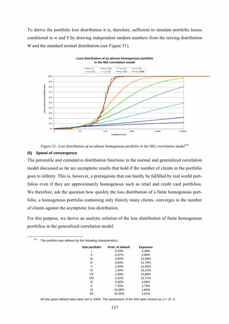
137

To derive the portfolio loss distribution it is, therefore, sufficient to simulate portfolio losses

conditional to w and Y by drawing independent random numbers from the mixing distribution

W and the standard normal distribution (see Figure 51).

Loss distribution of an almost homogenous portfolio in the NIG correlation model

0%

10%

20%

30%

40%

50%

60%

70%

80%

90%

100%

0,000010,00010,0010,010,11

Confidence level

Loss

in p

erce

nt o

f por

tfolio

val

ue

ρ = 0 ρ = 0,05 ρ = 0,2 ρ = 0,4ρ = 0,6 ρ = 0,8 ρ = 0,99 ρ = 0,9999

0 0.999990.99990.9990.990.9

Figure 51: Loss distribution of an almost homogenous portfolio in the NIG correlation model243

(5) Speed of convergence

The percentile and cumulative distribution functions in the normal and generalized correlation

model discussed so far are asymptotic results that hold if the number of clients in the portfolio

goes to infinity. This is, however, a prerequisite that can hardly be fulfilled by real world port-

folios even if they are approximately homogenous such as retail and credit card portfolios.

We therefore, ask the question how quickly the loss distribution of a finite homogenous port-

folio, a homogenous portfolio containing only finitely many clients, converges in the number

of clients against the asymptotic loss distribution.

For this purpose, we derive an analytic solution of the loss distribution of finite homogenous

portfolios in the generalized correlation model.

243 The portfolio was defined by the following characteristics:

Sub-portfolio Prob. of default ExposureI 0,33% 0,48%II 0,47% 3,96%III 0,65% 12,94%IV 0,83% 12,79%V 1,04% 21,55%VI 1,20% 15,21%VII 1,59% 10,86%VIII 2,02% 10,71%IX 3,30% 4,56%X 7,25% 2,73%XI 10,68% 1,60%XII 20,20% 2,61%

All loss given default rates were set to 100%. The parameters of the NIG were chosen as α = δ = 3.

138


ing an exposure of E = 1/n and risk index correlations 10 <≤ ρ the portfolio loss distribution

is given as

( ) ( ) ( ) ( )∑ ∫ ∫=

−−−

⋅⋅

−⋅⋅⋅−

Φ−⋅

−⋅⋅⋅−

Φ⋅

=

≤=

+

k

m

mnm

n

dwWdYYw

YwpFw

YwpFmn

nknp

nkL

0

11

11

1

Loss,/1,;

ϕρ

ρρ

ρ

ρ

R R

P

where ( )⋅ϕ is the standard normal density function and nk ,...,0∈ is the number of default-

ing clients in the portfolio.

Proof: In the generalized correlation model, in a homogenous portfolio client i defaults if

( )( )

ρρ

ρρ

−⋅⋅⋅−

≤⇔

≤⋅−⋅+⋅⋅=−

−

1

11

1

wYwpF

Z

pFZwYwX

i

ii

for ni ,...,1= .

Hence, client i’s probability of default conditional to Y and w is given as

( )

−⋅⋅⋅−

Φ=−

ρρ

1,|defaultsclient

1

wYwpF

YwiP


The conditional probability given w and Y that k of n clients default in the portfolio is then

simply defined by the binomial distribution

( ) ( )knk

wYwpF

wYwpF

kn

Ywnk

−−−

−⋅⋅⋅−

Φ−⋅

−⋅⋅⋅−

Φ⋅

=

=

ρρ

ρρ

11

1,|Loss

11

P

because clients are conditionally independent by assumption given w and Y.

This directly implies the loss distribution as stated in the theorem.

139

Figure 52 shows the loss distributions from Theorem 11 for various numbers of clients and

the asymptotic loss distributions for the normal and the NIG correlation model.

Normal correlation model(p = 0.5%, ρρρρ = 20%)

0%

10%

20%

30%

40%

50%

60%

70%

80%

90%

100%

1,E-081,E-071,E-061,E-051,E-041,E-031,E-021,E-011,E+00Confidence level

Loss

in p

erce

nt o

f por

tfolio

val

ue

Asymptotic PLD 1.000 clients 500 clients 100 clients 50 clients 10 clients

0 0.999990.99990.9990.990.9 0.99999990.999999 1 - 1E-8

NIG correlation model(p = 0.5%, ρρρρ = 20%, αααα = δδδδ = 2)

0%

10%

20%

30%

40%

50%

60%

70%

80%

90%

100%

1,E-081,E-071,E-061,E-051,E-041,E-031,E-021,E-011,E+00Confidence level

Loss

in p

erce

nt o

f por

tfolio

val

ue

Asymptotic PLD 1.000 clients 500 clients 100 clients 50 clients 10 clients

0 0.999990.99990.9990.990.9 0.99999990.999999 1 - 1E-8

Figure 52: The speed of convergence towards the asymptotic portfolio loss distribution in the generalized correlation model

It can be seen well that an increasing number of clients in the portfolio increases diversifica-

tion and reduces risk at all confidence levels. However, 500 clients seem to be sufficient to

fully exploit diversification effects and to approximately reach the asymptotic portfolio loss

distribution.

As a consequence, in many real world portfolios the lack of size in terms of numbers of cli-

ents cannot be the reason why analytic loss distributions for homogenous portfolios should

not be used for the calculation of portfolio risk. It is rather the lack of homogeneity within the

portfolio. Note, however, that all results discussed so far can be generalized to portfolios con-

sisting only of homogenous segments if the (heterogeneous) dependencies between the seg-

ments can be simulated. The over-all loss distribution is then merely a mixture of the analytic

loss distributions of the homogenous sub-portfolios. The previous section on almost homoge-

nous portfolios gave a simple example of how such a generalization could look like.

b) Estimation of risk index distributions

As we have shown in the previous sections, the choice of the risk index distribution signifi-

cantly influences the resulting loss distribution of a given portfolio. To control this type of

model risk it is, therefore, essential to employ a quantitative technique to estimate the risk

index distributions in dependence on the available risk index data.

A general approach to the estimation of risk index distributions could, for instance, make use

of non-parametric kernel smoothers. For simplicity, however, we supply a parametric estima-

140

tion technique244 under the assumption that the actual risk index distribution is an element of

the family of symmetric centered normal inverse Gaussian distributions.

Let d be the number of risk indices in the portfolio. For observations ni ,...,1= , let

( )miii xxx ,...,1= be a m-dimensional vector of realized values of these risk indices. The m-

dimensional symmetric centered NIG has the density

( ) ( ) ( ) ( )( )( ) 4/112

122/12

1

exp2

2,,,,; +−

−+

+

∆′+

∆′+

=∆ m

m

xx

xxmxnig

δ

δααδ

παδµδα δK

where ( ) 2/1+δK is the modified Bessel function of the third kind, 0, >δα , mR∈µ and

mm×∈∆ R is a positive definite matrix with determinant 1|| =∆ . Expectation and variance of

( )∆,,,,~ µδαmnigX can be shown to be given as

µ=XE

and

( ) ∆=Σ=αδ:XVar ,

i.e. ∆ is identical to the distribution’s covariance matrix Σ normed to have a determinant of

1:

m/1|| ΣΣ=∆

The estimation of the unknown parameters ∆,,, µδα proceeds in two steps. The first step

follows a method of moments approach245, i.e. we estimate the sample mean mR∈µ and the

sample covariance matrix mm×∈Σ Rˆ using standard techniques and get an estimate for ∆ as

m/1|ˆ|

ˆˆΣ

Σ=∆ .

To derive the remaining parameters δα and , a maximum likelihood approach can be used.

Standardizing the observations mix R∈ , ni ,...,1= , to iii xxy 1: −∆′= the log-likelihood func-

tion has the form

244 This approach was developed by Eberlein and Prause 1998 and Prause 1999. 245 Cf. Prause 1999, p. 108.

141

( ) ( ) ( ) ( )∑=

+

++−++

+++=n

iiim ymymnx

1

222/)1( ln

41ln

2ln

212ln,;L δδα

πααδδδα K

The log-likelihood function can be directly maximized using numerical techniques or first

derivatives can be calculated and set to zero.

With the abbreviation

( ) ( )( )x

xxλ

λλ K

KR 1: +=

and

( )( ) ( )xx

x λλλ RK −=′ln

the first derivatives are

( )∑=

+ ++−

++=n

iimi yymn

1

22/)1(

2

21L

dd δαδδα

R

and

[ ] ( )∑=

+− +

+−+=

n

iid

i

yy

n1

22/)1(2

1Ldd δα

δαδαδ

δR .

To verify that it is indeed a maximum which has been achieved and not some other stationary

point, second-order derivatives have to be examined.

With

( ) ( ) ( ) ( )( )x

xxxx 2

212:

λ

λλλλ K

KKKS ++ −=

and

( )( ) ( ) ( )2ln

xxxxx λλ

λλ −−=″ RSK

they are given as

( ) ( ) ( ) ( )∑=

++

+−

+

++−+−=

n

iim

i

imi y

y

yydn

1

22/)1(2

22/)1(2

22

2 1Ldd δα

δα

δαδ

ααS

R

142

( ) ( )∑=

++

+−

+

+−=

n

iim

i

im yy

yn

1

22/)1(2

22/)1(

2 2L

ddd δααδ

δα

δαδδα

SR

( ) ( )( )( ) ( )( )∑

∑

=

−−+

=+

−

++++−

+++−=

n

iiiim

n

iimi

yyy

yyn

1

2/3222/1222/)1(

1

22/)1(

122222

2

2

Ldd

δδδδα

δαδδαδδ

R

S

c) Copulas

A possibility to further generalize the correlation model beyond elliptic risk index distribu-

tions is not only to specify a model by one-dimensional margins of risk index distributions

and their linear correlations, but to employ copula functions246 to directly describe the

multivariate distribution of risk indices.

All information about the individual behavior and the dependence of real-valued random vari-

ables nXX ,...,1 is fully contained in their joint distribution function

( ) nnn xXxXxx ≤≤= ,...,,...,F 111 P

The objective to separate the joint distribution function into a part that expresses the marginal

distributions and another part that defines their dependence structure has led to the concept of

copula functions.

Definition:

A copula is the distribution function of a random vector in nR with uniform-(0, 1) marginals.

Let ( ) FXXX n ~...,,1= with continuous marginal distributions nFF ...,,1 . Then the copula C

of X is given as the joint distribution of ( ) ( )( )nn XFXF ...,,11 because ( ) ( )1,0~ UXF ii for

ni ...,,1= due to the percentile transformation:

( ) ( ) ( ) ( ) ( ) ( ) ( )( )nn

nnnn

nnn

xFxFCxFXFxFXF

xXxXxxF

,...,,...,

,...,,...,

11

1111

111

=≤≤=≤≤=

PP

The copula C of F is, thus, given as

246 For details on copula functions confer to Nelson 1999, Embrechts et al. 1999, or Embrechts et al. 2001.

143

( ) ( ) ( )( )nnn uFuFFuuC 11

111 ...,,...,, −−= .

If the joint distribution function F has continuous margins then the copula function C is

uniquely determined. It is intuitive to consider C as the dependence structure of F because C

is invariant under increasing continuous transformations of the marginals nFF ...,,1 .

Theorem 12247:

If ( )nXX ...,,1 has copula C and nTT ...,,1 are increasing continuous functions, then

( ) ( )( )nn XTXT ...,,11 also has copula C.

Bivariate normal copula

-4

-3

-2

-1

0

1

2

3

4

-4 -3 -2 -1 0 1 2 3 4

Bivariate nig-copula αααα = δδδδ = 0.25

-4

-3

-2

-1

0

1

2

3

4

-4 -3 -2 -1 0 1 2 3 4

x

y

Bivariate student-t-copula

1 degree of freedom

-4

-3

-2

-1

0

1

2

3

4

-4 -3 -2 -1 0 1 2 3 4

x

y

Figure 53: Bivariate distributions with standard normal marginals and different copulas

Figure 53 illustrates the effect of the copula function on the shape of the joint distribution.248

It clearly shows that the bivariate joint distribution is not uniquely determined by the mar-

ginals and their correlation. Note that only the bivariate normal distribution is elliptic while

both the NIG- and the t-copula induce a star-shaped joint distribution.

To demonstrate the effect of the copula on clients’ joint default probability if the joint distri-

bution is interpreted as the distribution of risk indices in analogy to the correlation model. The

5% default threshold is indicated in the graphs. Of the 1,000 sample points in each chart, 19

imply a joint default in the normal-correlation-model, 23 in the chosen NIG-correlation-

model, and 26 in the t-copula-correlation-model.

247 Cf. Embrechts et al. 2001, p. 5, theorem 1.6. 248 All marginal distributions are standard normal with correlation ρ = 0.6.

144

Although being a very desirable generalization of the correlation model described in the pre-

vious sections, the copula-correlation-model as we might call it, has two major drawbacks

which presently diminish its practical use significantly: firstly, the estimation of a high-

dimensional copula is a serious problem, especially if the available data is scarce249. Sec-

ondly, the concept of (linear) correlation, so inherent to the correlation model, is not entirely

defined on the level of the copula function, but also depends on the chosen marginals. For this

reason, it is sometimes difficult to find the correct parameterization of the copula to get the

desired risk index correlations. At this point, additional research has to be done to possibly

replace the concept of correlation by a more suitable and easy to handle measure of depend-

ence.

3. Random default probabilities (Credit Risk+ and Credit Portfolio View)

A more direct concept of dependence than in the correlation model is found in Credit Risk+

and Credit Portfolio View. Here it is explicitly assumed that clients’ default probabilities are

not constant, but vary as a function of some random systematic risk factors, and that clients

are independent conditional to the systematic factors.

a) Credit Risk+

In Credit Risk+ systematic risk factors are modeled as hidden variables that induce clients’

default probabilities to be gamma distributed with a given mean and variance250. In order to

be able to compute the portfolio loss distribution analytically, the authors of the model as-

sume that systematic risk factors only refer to the clients in a specific sector while risk factors

of different sectors are independent by supposition. Note that this presumption implies that

clients in different sectors are independent as well, a problematic concealed structural deci-

sion for a portfolio model. Only clients who are at least partially represented in the same in-

dustrial sectors appear to be dependent in their default behavior251.

Also for the sake of analytical solubility, the architects of the model sort clients into relatively

homogenous groups where all counterparties have the same default probability and volatility

and similar exposures. They also assume the number of clients defaulting in each group to be

Poisson distributed if a certain default probability is given.

249 See Embrechts et al. 1999, p. 3, for references. 250 See above section I.B.5 and CSFP 1996. 251 Hence, in order to have a certain basic dependence between all, say, corporate clients, a common sector would have

to be created where all corporate clients are represented. However, if such an approach is used, the definition of sec-tors in the model would deviate from firms’ industrial sectors and become somewhat artificial and difficult to quantify.

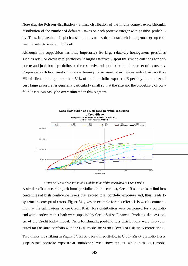
145

Note that the Poisson distribution - a limit distribution of the in this context exact binomial

distribution of the number of defaults - takes on each positive integer with positive probabil-

ity. Thus, here again an implicit assumption is made, that is that each homogenous group con-

tains an infinite number of clients.

Although this supposition has little importance for large relatively homogenous portfolios

such as retail or credit card portfolios, it might effectively spoil the risk calculations for cor-

porate and junk bond portfolios or the respective sub-portfolios in a larger set of exposures.

Corporate portfolios usually contain extremely heterogeneous exposures with often less than

3% of clients holding more than 50% of total portfolio exposure. Especially the number of

very large exposures is generally particularly small so that the size and the probability of port-

folio losses can easily be overestimated in this segment.

Loss distribution of a junk bond portfolio according to CreditRisk+

Comparison: CRE model for different correlations ρρρρ(portfolio value = 130.512.072 EUR)

0

50.000.000

100.000.000

150.000.000

200.000.000

0,00010,0010,010,11

Confidence level

Loss

ρ = 0 ρ = 10% ρ = 20% ρ = 30% ρ = 40% ρ = 50%ρ = 60% ρ = 70% ρ = 80% ρ = 90% Credit Risk + Limit percentile

0 0.99990.9990.990.9

Figure 54: Loss distribution of a junk bond portfolio according to Credit Risk+

A similar effect occurs in junk bond portfolios. In this context, Credit Risk+ tends to find loss

percentiles at high confidence levels that exceed total portfolio exposure and, thus, leads to

systematic conceptual errors. Figure 54 gives an example for this effect. It is worth comment-

ing that the calculations of the Credit Risk+ loss distribution were performed for a portfolio

and with a software that both were supplied by Credit Suisse Financial Products, the develop-

ers of the Credit Risk+ model. As a benchmark, portfolio loss distributions were also com-

puted for the same portfolio with the CRE model for various levels of risk index correlations.

Two things are striking in Figure 54. Firstly, for this portfolio, in Credit Risk+ portfolio losses

surpass total portfolio exposure at confidence levels above 99.35% while in the CRE model

146

the maximum portfolio loss is always given by total portfolio exposure as it should be in a

framework where the portfolio exposure is not subject to risk itself.

Secondly, the portfolio loss distribution produced by Credit Risk+ is much more continuous

than the portfolio loss distribution resulting from the CRE model. This effect is again a con-

sequence of the assumed Poisson approximation in Credit Risk+ because it implies that not

only the large, but also the small individual exposures in the portfolio can default in an arbi-

trarily large number. Hence, the big jumps in the portfolio loss distribution caused by the de-

fault of a large exposure will be filled up.

It is worth noting, though, that these conceptual pitfalls in Credit Risk+ have their origin in a

number of decisions that were exclusively made for analytical tractability of the model. All of

them could easily be avoided if computer simulations were allowed to solve the model.

b) Credit Portfolio View

As already described in section I.B.6.b) above, in Credit Portfolio View a segment’s condi-

tional probability of default252 given a macroeconomic situation and a random shock is

( )τεθε

++=

XXp

exp11,|

where X is a vector of macroeconomic factors, ε a standard normal random innovation, θ a

parameter vector and τ a scalar parameter.

4. A brief reference to the literature and comparison of the models ap-plied to homogenous portfolios

The discussion in the previous sections has shown that there are numerous differences be-

tween the leading credit portfolio models in terms of relevant input factors and their estima-

tion and of modeling assumptions. Also sometimes conceptual errors and imprecisions may

occur in one model, but not in the others. As a consequence, it is highly likely that the models

will lead to very different results even if they are applied to the same portfolio.

However, there is a major current in the literature253 that intends to place the models within

the same mathematical framework and tries to show that the models lead to practically

equivalent results, if the input parameters are harmonized properly implying “that relative

252 At this point, we ignore the unpublished derivation of conditional transition probabilities for different rating grades and

industrial sectors and consider all speculative grade companies in the same sector as one segment. 253 See for instance Koyluoglu and Hickman 1998 and Gordy 2000.

147

‘theoretical correctness’ need not rank among a user’s model selection criteria, which might

then consist primarily of practical concerns…”254.

Koyluoglu and Hickman find a common mathematical framework in the fact that clients’ de-

faults are conditionally independent in all models given the respective set of systematic risk

factors. This conceptual phenomenon is a general feature of all structural risk models, though,

not only of credit risk models, that does not give any hint concerning a model’s ‘theoretical

correctness’.

What is more, calculation results can sometimes be subject to interpretation errors. For in-

stance, Koyluoglu and Hickman calculate the distributions of conditional default probabilities

given the respective set of systematic risk factors for a standardized type of firm255 with the

normal correlation model, Credit Risk+ and Credit Portfolio View. To compare the resulting

distributions, they defined a ‘tail-agreement statistics’

( )( ) ( )

( ) ( )∫∫

∫∞∞

∞

−

−−=Ξ

zz

zz

xxgxxf

xxgxfgf

dd

d||1,

where f and g are density functions of two distributions of conditional default probabilities to

be compared and z defines the beginning of the ‘tail’256. Koyluoglu and Hickman define the

tail as the area more than two standard deviations above the mean of the distributions of con-

ditional default probabilities, i.e. z = p + 2σ and get

ΞΞΞΞNCM vs. CPV 94.90%NCM vs. CR+ 93.38%CPV vs. CR+ 88.65%

which they take as an indication for the similarity of the models257.

To see that this conclusion might be misleading for the standard portfolio statistics such as

value at risk and shortfall and be due to the ‘tail-agreement statistics’ used for the comparison,

note that in homogenous portfolios with a total exposure of 1 the distribution of conditional

254 Koyluoglu and Hickman 1998, p. 18. 255 They consider firms with an unconditional default probability p = 1.16% and a standard deviation of the conditional de-

fault probability of σ = 0.9%. They chose these parameter values to match Moody’s ‘All Corporate’ default experience for 1970-1995, as reported in Carty and Lieberman 1996. See Koyluoglu and Hickman 1998, p. 12ff.

256 Koyluoglu and Hickman 1998, p. 18. 257 Koyluoglu and Hickman 1998, p. 14f.

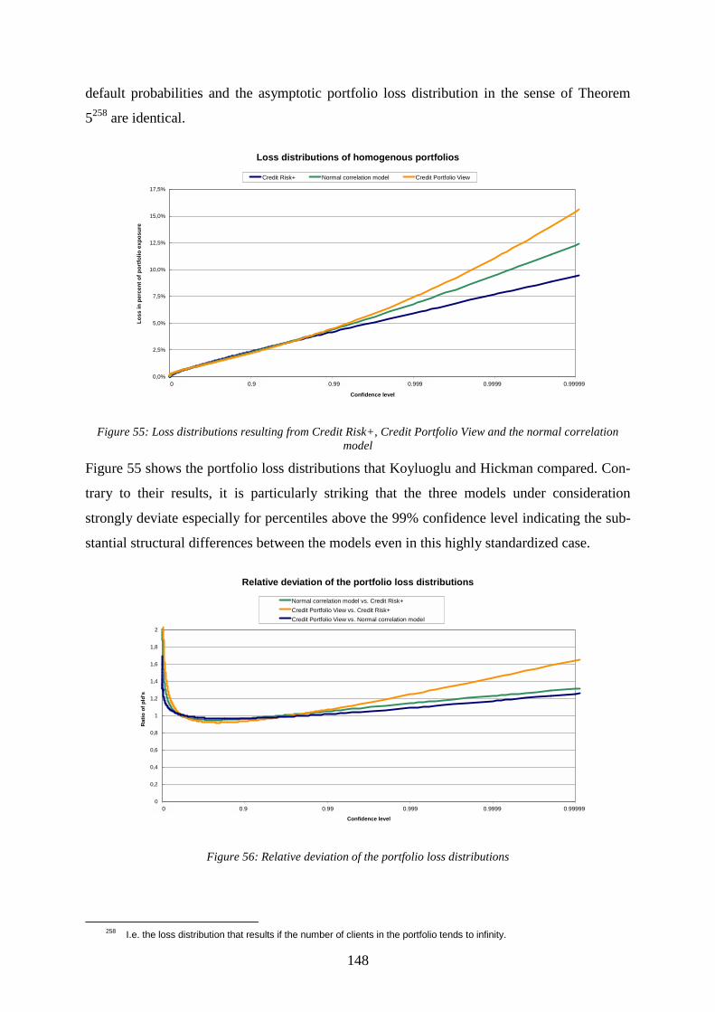
148

default probabilities and the asymptotic portfolio loss distribution in the sense of Theorem

5258 are identical.

Loss distributions of homogenous portfolios

0,0%

2,5%

5,0%

7,5%

10,0%

12,5%

15,0%

17,5%

0,000010,00010,0010,010,11

Confidence level

Loss

in p

erce

nt o

f por

tfolio

exp

osur

e

Credit Risk+ Normal correlation model Credit Portfolio View

0 0.999990.99990.9990.990.9

Figure 55: Loss distributions resulting from Credit Risk+, Credit Portfolio View and the normal correlation model

Figure 55 shows the portfolio loss distributions that Koyluoglu and Hickman compared. Con-

trary to their results, it is particularly striking that the three models under consideration

strongly deviate especially for percentiles above the 99% confidence level indicating the sub-

stantial structural differences between the models even in this highly standardized case.

Relative deviation of the portfolio loss distributions

0

0,2

0,4

0,6

0,8

1

1,2

1,4

1,6

1,8

2

0,000010,00010,0010,010,11

Confidence level

Rat

io o

f pld

's

Normal correlation model vs. Credit Risk+Credit Portfolio View vs. Credit Risk+Credit Portfolio View vs. Normal correlation model

0 0.999990.99990.9990.990.9

Figure 56: Relative deviation of the portfolio loss distributions

258 I.e. the loss distribution that results if the number of clients in the portfolio tends to infinity.

149

At the 99.9% confidence level, that was chosen as the standard measure of credit portfolio

risk by the Basel Committee for Banking Supervision259, we find the following relative devia-

tions between the loss distributions (Figure 56):

99.9%-VaR 99.9%-ShortfallCPV vs. NCM 9.07% 12.90%NCM vs. CR+ 14.37% 18.43%CPV vs. CR+ 24.73% 33.71%

and, thus, a divergence of from 9% to almost 25% between the 99.9%-values at risk and a

12.9% to 33.7% discrepancy between the 99.9%-shortfalls.

This evidence clearly shows that superficial mathematical similarities between models do not

at all imply resemblance from the risk managers point of view.

5. Event driven dependencies (CRE model)

A complementary concept of dependence between clients in credit portfolios is event driven.

Examples could be country risk and microeconomic risks between individual counterparties.

Event driven dependencies occur if a client’s ability to repay a credit or any other obligation

is directly affected if a certain incident arises or not260.

For instance, creditors who are resident abroad can only serve their debts if international

money transfers are not interrupted for reasons such as political or economic crises or the lo-

cal central bank’s lack of foreign currencies. The probability of the disruption of a country’s

international money transfers is typically measured by the countries rating as it is supplied by

the international rating agencies such as Moody’s, Standard & Poor’s and Fitch’s.

The other canonical illustration for event driven risks is microeconomic dependency between

individual clients. Take for example a firm who has only one customer. An insolvency of its

single purchaser would certainly not leave the firm unaffected, but force it to quickly find one

or more new clients to avoid default itself.

259 See BCBS 2001. 260 For details see also section I.B.7.a)(2) above.

150

The event risk effect in portfolio risk calculations

0%

5%

10%

15%

20%

0,00010,0010,010,11

Confidence level

Loss

in p

erce

nt o

f por

tfolio

exp

osur

e

including country risk ignoring country risk

0 0.99990.9990.990.9

Figure 57: The event risk effect in portfolio risk calculations: country risk

Figure 57 demonstrates the effect of the inclusion of country risk in the calculation of portfo-

lio risk. In the example, 10% of all clients in an otherwise homogenous portfolio261 lodge

abroad. The probability of an interruption of money transfers is set to 0.2%. Due to the homo-

geneity of the portfolio, the loss distribution is not discontinuous, but steeply rises before

0.2% to incorporate the additional loss caused by country risk.

Opposite to risk index correlations or random default probabilities, it is a characteristic feature

of event risks that they can model asymmetric dependencies between portfolio components.

In case of country risk an interruption of money transfers between a country and the rest of

the world simultaneously affects all clients who lodge in that country. An insolvency of a cli-

ent in that country, however, usually does not affect the country’s ability to transfer money.

Although a counterparty’s ability to participate in international business decisively depends

on the quality of his home country, this is not true vice versa.

In case of microeconomic dependencies between firms, dependencies may be positive in both

directions and of different size. Moreover, since clients can affect each other in this setting,

the influence of microeconomic dependencies on portfolio risk can be modeled in several

rounds leading to a cascading effect. In round 0 portfolio risk is calculated as if no microeco-

nomic dependencies were present in the portfolio finding a certain number of defaults. In

round 1 the consequences of these defaults are analyzed. Due to individual dependencies of

clients who are not in insolvency so far (in the model) on defaulted business partners some of

261 Clients’ individual default probability is p = 0.5% with correlations of ρ = 20% in the normal correlation model.

151

the still intact clients will be drawn into the crisis and default in turn. Round 2 proceeds simi-

larly and investigates the effect of these new collapses and so on.

Probability of contamination ππππ = 25%

0%

5%

10%

15%

20%

25%

30%


Loss

in p

erce

nt o

f por

tfolio

exp

osur

e

n = 0 n = 1 n = 2 n = 3 n = 4 n = 5 n = 6 n = infinity

0 0.999990.99990.9990.990.9


0%

5%

10%

15%

20%

25%

30%

35%

40%


Loss

in p

erce

nt o

f por

tfolio

exp

osur

e


0 0.999990.99990.9990.990.9


0%

5%

10%

15%

20%

25%

30%

35%

40%

45%

50%


Loss

in p

erce

nt o

f por

tfolio

exp

osur

e


0 0.999990.99990.9990.990.9


0%

10%

20%

30%

40%

50%

60%

70%


Loss

in p

erce

nt o

f por

tfolio

exp

osur

e


0 0.999990.99990.9990.990.9

Figure 58: Cascading effect of microeconomic dependencies

Figure 58 gives an impression of the cascading effect of microeconomic dependencies on a

homogenous portfolio262. For the first few rounds, the effect is significant even for small

probabilities of contamination increasing drastically with the contamination probability.

However, note that independent of the contamination probability the total cascading effect

converges towards a limiting distribution if the number n of rounds tends to infinity.

262 Clients are assumed to have a default probability of 0.5% and risk index correlations of 20% in the normal correlation

model. The portfolio was constructed so that each client affects exactly one other client, e.g. client 1 affects client 2, client 2 affects client 3 and so on. We define the contamination probability as the probability that a defaulting clients draws another clients who is related to him into insolvency as well.

Then, given a proportion of 0a of defaulting clients in the portfolio, round n leads to an additional fraction of

( )∑−⋅⋅==

+

n

iinn aaa

01 1π

of defaulting clients. The total cascading effect 1+nc is then

∑=+

=+

1

01

n

iin ac .

152

B. Time horizons for risk calculations

Bank portfolios usually comprise of credits and trades of strongly heterogeneous maturities. It

is, therefore, not a matter of course to choose a single time horizon for portfolio risk calcula-

tions. Depending on the characteristics of the portfolio under consideration and the purpose of

the risk analysis, a standardized time horizon for the entire portfolio or individual maturities

for the single exposures and positions may be appropriate. Estimation of economic capital

requirements puts the focus on a continuously renewing portfolio and, therefore, selects a

normalized time frame for the entire portfolio. Conversely, e.g. the valuation of basket credit

derivatives fixes a portfolio consisting of specific exposures and asks for potential losses until

the maturity of the last position in the portfolio. In this context, a heterogeneous time scheme

that is adapted to the maturity of the single exposures in the basket is suitable.

1. A standardized time horizon

If a portfolio analysis is performed in order to compute economic capital requirements an arti-

ficial, standardized time horizon for all portfolio components independent of their actual re-

maining time to maturity applies for two reasons:

Firstly, the fundamental concept of portfolio risk, all widely used risk measures such as ex-

pected loss, value at risk, shortfall and standard deviation are based upon, tracks the variation

of portfolio losses within a certain amount of time. Hence, a standardized time frame is im-

manent to this notion of risk.

Secondly, portfolio structures are much more stable than isolated portfolio components. For

instance, a six months money market loan ceases to exist after half a year. The total quantity

of six months credits will habitually hardly have changed, though, because firms and financial

institutions have a permanent need of short term finance. Figuratively speaking, the portfolio

of a constantly operating bank can be seen as a lake that permanently changes its water, but

remains more or less steady over time.

The choice of a standardized time horizon implicitly assumes that the portfolio manager is not

predominantly interested in the single client’s credit risk, even if it is possible to break down

total portfolio risk to the level of a single client’s risk contribution263, but mainly in the risk

level of the portfolio as a whole. For that reason, the practical supposition is made that a client

who leaves the portfolio because his trades and credits have expired or because his position

263 See below section II.D.1.

153

has been sold is always replaced by another client of approximately the same type, i.e. of the

same credit worthiness, exposure, country, sector etc.

Following the accounting period and the rating update scheme, most banks choose a one-year

time frame for their portfolio risk calculations. However, if the appropriate input data is used,

e.g. default and transition probabilities, exposures, other intervals are possible. Figure 59 puts

on view how the 99.9%-value at risk increases with the time horizon for various one-year

probabilities of default.

Influence of the time horizon on the 99.9%-value at risk(homogenous portfolio in the normal correlation model, ρρρρ = 20%)

0%

10%

20%

30%

40%

50%

60%

70%

80%

90%

100%

0 1 2 3 4 5 6 7 8 9 10

Time horizon

99.9

%-v

alue

at r

isk

in p

erce

nt o

f por

tfolio

exp

osur

e

p = 0.1% p = 0.5% p = 1% p = 2% p = 5%

Figure 59: Influence of the time horizon on the 99.9%-value at risk

In order to be able to consider long time horizons, it is essential to be capable of providing the

corresponding default probabilities. In the exhibit, we chose one-year default probabilities p

and extrapolated them to arbitrary time horizons assuming that clients’ defaults follow a

Markov process, i.e. that the probability to go into bankruptcy in the time interval from t to

t+1 is constant at 1

pp = provided that a client did not default until time t. A client’s probabil-

ity tp to default in the time interval between 0 and t then is

( ) tt

pp1

11 −−= .

In reality, this Markov assumption, that greatly facilitates the derivation of long term default

probabilities, is only a very rough approximation of clients’ true default processes as a com-

parison of the resulting probabilities with directly estimated probabilities, e.g. by rating agen-

cies, reveals.

154

Long term investment grade default rates (Moody's direct estimates versus extrapolated one-year dp's)

0,0%

0,5%

1,0%

1,5%

2,0%

2,5%

3,0%

3,5%

4,0%

1 3 5 7 9 11 13 15

Time horizon

Def

ault

rate

AAA - Moody's AA - Moody's A - Moody's BBB - Moody's Inv. - Moody'sAAA - extra. AA - extra. A - extra. BBB - extra. Inv. - extra.

Long term speculative grade default rates (Moody's direct estimates versus extrapolated one-year dp's)

0%

10%

20%

30%

40%

50%

60%

70%

80%

90%

100%

1 3 5 7 9 11 13 15

Time horizon

Def

ault

rate

BB - Moody's B - Moody's CCC - Moody's Spec.grade - Moody'sBB - extra. B - extra. CCC - extra. Spec.grade - extra.

Figure 60: Term structure of default rates: direct estimates versus extrapolated values

Figure 60 compares Moody’s estimates264 of long term default rates with the respective ex-

trapolated values. The extrapolated default probabilities turn out to be consistently and con-

siderably lower than the directly estimated values for investment grade ratings up to BB while

they are significantly higher for speculative grade firms. Note that this deviation inevitably

carries over to the calculation of portfolio risk.

This example shows that long time horizons should only be chosen very carefully because the

direct estimation of long term default rates, which is also essential to calibrate extrapolation

techniques, requires an increasingly long history of default experience. Otherwise the preci-

sion of portfolio risk calculations would suffer to a great extent.

264 See Moody’s 2000, p. 16, table 11.

155

2. Heterogeneous time horizons

A very different situation is given if the portfolio does not permanently renew itself, but is a

fixed set of gradually expiring exposures. This is, for instance, the case of basket credit de-

rivatives. Here, a financial institution sells the losses coming off a certain portfolio of expo-

sures, usually except a ‘first loss piece’ that still has to be carried by the vendor of the deriva-

tive.

A typical way to value this kind of credit derivative is to calculate the basket’s expected ex-

cess loss over the first loss piece until maturity of the last position in the basket, i.e. the ex-

pected shortfall corresponding to the first loss piece. Here a standardized time horizon would

apparently distort the results. Instead, risk calculations have to be performed successively

over multiple periods until the last maturity has been reached which includes in each step only

those exposures that don’t have expired or defaulted before. Note, however, that the difficul-

ties in estimating long term default probabilities, that were described in the previous section,

naturally remain the same in this context.

C. Quantification of portfolio risk

Having specified the clients’ default probabilities, exposures, recovery rates and interdepend-

encies and the relevant time horizon for each position and the entire portfolio, the portfolio

model is fully defined. The next task is the quantification and analysis of portfolio risk

through the portfolio loss distribution and various risk measures, which focus on certain char-

acteristics of the loss distribution.

We begin the section with a discussion of the calculation of the portfolio loss distribution and

the construction of confidence intervals. We will then define risk measures based upon the

previously derived loss distribution, show how they can be estimated and used in practice and

discuss the properties of the estimators.

1. Portfolio loss distribution

The main result of the quantitative portfolio risk analysis is the calculation of the portfolio

loss distribution or, more precisely, of the cumulative portfolio loss distribution function, i.e.

of the function

( ) xx ≤= lossportfolioL P .

156

The loss distribution contains all information about portfolio risk at the aggregate level and is

also a central component of the analysis of the composition of portfolio risk.

In most portfolio models, the analytical calculation of the loss distribution is tremendously

difficult due to the complex interrelations of portfolio components. However, the loss distri-

bution can be approximately derived through Monte-Carlo-simulation techniques. Here, n

random portfolio losses nXX ,...,1 are drawn as independent realizations from the portfolio

loss distribution and the empirical loss distribution function is calculated as

( ) ∑≤

=xXi

ini

Xn

x:

1L .

Note that ( )xnL depends on the simulated random portfolio losses nXX ,...,1 and is, there-

fore, random itself. Nonetheless, the empirical loss distribution function can be used to esti-

mate the portfolio loss distribution because it uniformly converges towards the true portfolio

loss distribution with probability one:

Theorem 13 (Glivenko-Cantelli):

Let nXX ,...,1 be independent realizations of the random variable X with cumulative distribu-

tion function ( )xL . Let ( )xnL be a realization of the empirical distribution function implied

by nXX ,...,1 . Then

( ) ( ) 10|LL|suplim =

=−

+∞<<∞−∞→xxn

xnP .

Uniform 95%-confidence bands for the portfolio loss distribution(dp = 0.5%, ρρρρ = 30%)

0%

5%

10%

15%

20%

25%

30%

35%

40%

0,00010,0010,010,11

Probability to exceed the stated loss

Loss

in p

erce

nt o

f por

tfolio

exp

osur

e

PLD 1000 runs 10000 runs100000 runs 1000000 runs 10000000 runs

0 0.99990.9990.990.9

Figure 61: Uniform 95%-confidence bands for the portfolio loss distribution dependent on the number of simu-lation runs

157

Figure 61 shows the portfolio loss distribution of a homogenous portfolio in the normal corre-

lation model265 and uniform confidence bands for the empirical loss distribution dependent on

the number of simulation runs266. The confidence bands can be interpreted that with a prob-

ability of 95% the entire empirical loss distribution will be within the region between the up-

per and the lower band. It is evident from the exhibit that the probability of small portfolio

losses can well be estimated even with a small number of draws from the loss distribution.

Conversely, in order to get a good fit at high percentiles of the loss distribution, a compara-

tively large number of simulation runs is necessary.

We get a qualitatively similar, but quantitatively more moderate result, if we do not look at

uniform confidence bands, i.e. at the supreme of the deviations of the empirical from the true

loss distribution over all x, but at the pointwise deviation of ( )xnL from ( )xL .

Pointwise 95%-confidence intervals for the portfolio loss distribution(dp = 0.5%, ρρρρ = 30%)

0%

5%

10%

15%

20%

25%

30%

35%

40%

0,00010,0010,010,11

Confidence level

Loss

in p

erce

nt o

f por

tfolio

exp

osur

e

PLD 100 runs 1000 runs 10000 runs 100000 runs

0 0.99990.9990.990.9

Figure 62: Pointwise 95%-confidence intervals for the portfolio loss distribution dependent on the number of simulation runs

Here, the focus is not at the entire loss distribution at once, but rather at every percentile of

the distribution separately. The confidence intervals state that a given percentile of the em-

pirical loss distribution will lie in the specified range with a probability of 95%. It may hap-

pen, though, that an empirical distribution function is inside the confidence intervals for some

x while it is outside for others.

265 We assume that the portfolio exposure is split among an infinite number of clients. See above Theorem 2. 266 The asymptotic portfolio loss distribution is absolutely continuous with respect to Lebesgue-measure so that the statis-

tic

( ) ( ) ||sup xLxLd nx

n −=∈ R

has a Kolmogorov-Smirnov-distribution, which can be used to calculate the confidence bands.

158

We see that the pointwise convergence of the empirical loss distribution to the true one occurs

much faster than the uniform convergence especially in the tail of the distribution. The exact

speed of convergence for the case of continuous loss distributions is stated in the next theo-

rem.

We begin with a definition.

Definition: Let

( ) ( ) ( )nXXX ≤≤≤ ...21

be the order statistic of the random draws from the loss distribution, and let

( ) ( )

( ) ∈

=+

−

elseif

:L1pn

pnn X

pnXp

N

be the empirical inverse cumulative portfolio loss distribution function267 for 10 << p .

Theorem 14 (Bassi, Embrechts, Kafetzaki) 268:

Assume that the true portfolio loss distribution L is continuous with density ( )xf and inverse

cumulative distribution function ( )p1L− for 10 << p . Then

( ) ( ) ( )( )( )

⋅−−

−−

pfnppppn 12

1

L1;L~L N

for large n if ( )( ) 0L 1 >− pf .

Thus, the pointwise estimation of the portfolio loss distribution is not only consistent in n as

was already implied by Theorem 13, but the stochastic convergence is of order

nO 1 .

However, the variance of the percentile estimator ( )pn−L does not only crucially depend on

the number of simulation runs n, but also on the value of the density of the loss distribution at

the true percentile ( )p1L− . Since the likelihood p−1 of extremely large portfolio losses is

typically very small in credit risk management with equally small values of ( )( )pf 1L− , this

implies that the efficiency of the pointwise estimation of the portfolio loss distribution usually

267 np is defined as the largest integer npm ≤ . 268 See Bassi et al. 1998, p. 117.

159

declines in p for values of p close to 1 leading to larger confidence intervals for a given num-

ber of simulation runs (see Figure 62).

In the above examples, we assumed that the portfolio loss distribution is known and continu-

ous and, in order to illustrate the natural variation in simulation results, we derived analytic

confidence bands and confidence intervals that comprise the simulated loss distribution with a

given probability.

In practical applications, we have the opposite situation that the true loss distribution is un-

known and usually discontinuous. In this case, pointwise (random) confidence intervals for

the true loss distribution can be calculated from the simulated loss distribution.

For any ( )1,0∈p the p-percentile of a general loss distribution can be estimated through the

inverse empirical cumulative loss distribution defined above. Let the random variable Y = 0 if

a random draw from the loss distribution is smaller than or equal to ( )p1L− . By definition269

of the p-percentile,

pqY ≥== 0P .

If the loss distribution is continuous, pq = for all p. If, on the other hand, the loss distribu-

tion has discrete parts, there may be some p so that pq > . These are the portfolio losses x

where the loss distribution L has point masses, namely the discontinuity points of L. Since we

do not know the true loss distribution, the exact value of q is unknown in these cases.

Nevertheless, we can conclude that the number of random draws from the loss distribution

that are smaller than or equal to ( )p1L− is binomially distributed with parameters q and n, if

the experiment is repeated n times. Hence, a confidence interval for ( )p1L− with confidence

level α can be constructed by choosing indices j and k so that

( ) ( ) ( ) ( )∑−

=

−− ≥−

=<≤

11 1

k

ji

inikj qq

kn

XpLX αP

with ( ) ( ) ( )knj XpLX <≤ − . These confidence intervals would be exact if we knew the value of

q. We can use these exact confidence intervals that use the unknown parameter q to derive

approximate and slightly conservative confidence intervals that are dependent on p and α

alone.

269 The p-percentile is defined as ( ) pxxp ≥≤=

−loss:inf:L

1 P .

160

For large270 n the binomial distribution can be approximated by the normal distribution since

( )( )xx

qnq

nqYn

ií

nΦ=

≤−

−∑=

∞→ 1lim 1P

due to the central limit theorem. With

( )( )az

a

a1

2/11−Φ=−−= α

and functions

( )

+∈

=else1

if:,

pnpnpn

npcN

( ) ( ) ( ) ( )( ) ( )

−⋅−∈−⋅−⋅−

=else1

1if1:,

pnpzpcpnpzpnpzpc

npda

aa N

( ) ( ) ( ) ( )( ) ( )

+−⋅+∈−⋅−⋅+

=else11

1if1:,

pnpzpcpnpzpnpzpc

npea

aa N

symmetric confidence intervals for ( )p1L− with confidence level α are implied from

( )( ) ( ) ( )( ) α≥<≤ −nqenqd XpLX ,

1,P .

Note that ( ) ( )npcpn ,L =− is a consistent estimator of ( )p1L− due to Theorem 13. Moreover,

the standard deviation ( )pnp −1 of the asymptotic normal distribution of ∑=

n

iiY

1

falls strictly

monotonously in 2/1≥p so that

( ) ( )qnqpnp −≥− 11

for 2/1≥p . Conservative symmetric confidence intervals for ( )p1L− with confidence level α

are, hence, given as

( )( ) ( ) ( )( ) α≥<≤ −npenpd XpLX ,

1,P .

270 As a rule of thumb, the approximation works well if ( ) 91 >− pnp .

161

For 2/1<p the calculation of confidence intervals is less problematic because this part of the

portfolio loss distribution is much less relevant for risk management purposes. In addition,

loss distributions are usually more continuous in the region of low losses than in the tail. This

means that the above approximation is unlikely to largely underestimate confidence intervals

when used for values of 2/1<p . With

( ) ( )( )

+⋅−∈⋅⋅−=

else12/2/if2/:,

nzpcnznzpcnpg

a

aa N

( ) ( )( )

+⋅+∈⋅⋅+=

else12/2/if2/:,

nzpcnznzpcnph

a

aa N

conservative confidence intervals can be obtained for 2/1<p as

( )( ) ( ) ( )( ) α≥<≤ −nphnpg XpLX ,

1,P .

In order to condense and to interpret the information contained in the portfolio loss distribu-

tion, risk measures are defined that are entirely based upon the previously calculated loss dis-

tribution and are conceptually identical in all risk models. In the following sections we define

and discuss the expected loss, the portfolio standard deviation, the value at risk, and the short-

fall.

2. Expected loss

The expected portfolio loss is the most elementary risk measure. It is defined as the expected

value of the portfolio loss distribution. The most important characteristic of the expected loss

is that it is always the sum of the expected losses of the portfolio components and, thus, can-

not be diversified. This is why it can be considered as the basic risk of a portfolio that has to

be covered by risk premiums under all circumstances, if the financial institution does not want

to expect a loss from its portfolio that is not accessible to risk management otherwise.

a) Estimation

Let nXX ,...,1 be the simulated independent draws from the portfolio loss distribution. Then

the expected loss µ can be unbiasedly and consistently estimated through the arithmetic mean

of the simulated loss distribution:

162

( ) ∑=

=n

iin X

nXX

11

1,...,µ

and we have

(unbiasedness) ( )[ ] [ ] µµ == ∑=

n

iin X

nXX

11

1,...,ˆ EE

and

(consistency) ( ) 0|,...,ˆ|lim 1 =>−∞→

εµµ nnXXP

for all 0>ε .

b) Confidence intervals

It follows from the central limit theorem, that ( )nXX ,...,ˆ 1µ is asymptotically normally dis-

tributed with mean µ and standard deviation

( )n

nn

Xn

XX

n

ii

σσσσ µ === ∑=

2

1

2ˆ

11ˆ

where Xσ is the standard deviation of the portfolio loss distribution. Xσ can be consistently

estimated as

( )( )∑=

−−

=n

iniX XXX

n 1

21,...,ˆ

11ˆ µσ

(see section II.C.3.a) below).

Upper and lower limits of confidence intervals at the confidence level α for the expected loss

then are

( ) µµ σµ ˆ1 ˆ,...,ˆCI ⋅±= an zXX

with

( ) ( )aza a1and2/11 −Φ=−−= α .

163

Analytically calculated expected loss and confidence intervals

0,0%

0,1%

0,2%

0,3%

0,4%

0,5%

0,6%

0,7%

0 10.000 20.000 30.000 40.000 50.000 60.000 70.000 80.000 90.000 100.000

Simulation runs

Loss

in p

erce

nt o

f por

tfolio

exp

osur

eLower 95%-CI Expected Loss Upper 95%-CI Span

Expected loss estimated from simulation results and confidence intervals

0,0%

0,1%

0,2%

0,3%

0,4%

0,5%

0,6%

0,7%

0 10.000 20.000 30.000 40.000 50.000 60.000 70.000 80.000 90.000 100.000

Simulation runs

Loss

in p

erce

nt o

f por

tfolio

exp

osur

e

Lower 95%-CI Expected Loss Upper 95%-CI Span True value

Figure 63: Accuracy of the estimation of the expected portfolio loss dependent on the number of simulation runs

Figure 63 shows the analytic and simulated results for the expected loss and confidence bands

for the estimator at the 95%-confidence level for a homogenous portfolio with default prob-

ability 0.5% and risk index correlations of 30% in the normal correlation model. The span is

defined as the difference between the upper and the lower bound of the confidence interval.

To get the simulated values of the expected loss and its confidence intervals in the right chart,

the distribution of the estimator was simulated 1,000 times and the mean, the 2.5%-percentile

and the 97.5%-percentile were plotted271.

It is evident from the exhibits that the simulation results are well in line with the analytic solu-

tion and that the estimation of the expected loss is unbiased for all numbers of simulation

runs. Note as well that the span of the confidence intervals decreases strictly monotonously in

the number of simulation runs as would be expected from the consistency of the estimator, but

that the increase in precision from an additional run declines rapidly.

3. Standard deviation272

The portfolio standard deviation is another widely used risk measure. It is defined as the stan-

dard deviation of the portfolio loss distribution. Other than the expected loss, the size of the

portfolio standard deviation changes with the composition of the portfolio even if the portfo-

lio’s expected loss is held constant. Hence, by considering clients’ marginal contributions to

the portfolio standard deviation, the standard deviation can be used to analyze the portfolio

structures and to localize components that are well diversified in the portfolio and others

where risk is particularly concentrated.

271 Two simulations were performed sequentially. First, a sample of n points was drawn from the portfolio loss distribution

and the expected value was estimated as described above. Then, this was repeated 1,000 times in order to obtain 1,000 independent estimates for the expected loss as an empirical proxy for the distribution of the estimator.

272 On the applicability of the portfolio standard deviation in credit risk management confer to Wehrspohn 2001.

164

One of the major advantages of the standard deviation that founded its popularity among prac-

titioners is that it is analytically computable in elementary portfolio models such as the Va-

sicek-Kealhofer model273. In more complicated models such as the CRE model where several

influences on the clients’ credit risk superimpose one another such as country risk, sectorial

correlations and individual dependencies with other clients, the analytical calculation of the

portfolio standard deviation is considerably more complicated and no longer practicable. Be-

low we show how the standard deviation and confidence intervals can be estimated based on

the simulation results.

A second great advantage of the portfolio standard deviation is that it expresses a feature of

the entire loss distribution. This is particularly valuable if it comes to the calculation of the

individual clients’ contributions to total portfolio risk because for a client with positive prob-

ability of default and positive exposure his marginal standard deviation is also positive. This

is not necessarily the case with a client’s marginal value at risk or shortfall which much

stronger depend on the specific simulation results and the number of simulation runs per-

formed since they only consider a specific percentile or the tail of the loss distribution, respec-

tively.

However, in all credit risk models, the standard deviation has the important drawback that it

cannot be interpreted easily. This is a decisive difference between the application of portfolio

standard deviation in the risk management of, say, equity portfolios as compared to the risk

management of credit portfolios. In popular equity portfolio models such as the capital asset

pricing model (CAPM), the distribution of portfolio returns is always a normal distribution so

that there is a constant ratio between portfolio standard deviation and any value at risk to a

constant confidence level. For example, no matter how the portfolio is composed, the 99%-

value at risk is always 2.32 standard deviations above the mean in a normally distributed set-

273 In general, the portfolio variance is the sum of the variances and covariances of the portfolio components and can be

written as

( ) ( )∑∑∑∑= == =

−−==k

i

k

jjjiiji

defij

k

i

k

jij pppp

1 11 1

22 11ηηρσσ

where k is the number of clients in the portfolio, ip is the default probability of client i for ki ,...,1= , iη his exposure,

and defijρ the default correlation between client i and j. In the Vasicek-Kealhofer model the default correlation def

ijρ can be directly computed as

( ) ( )( )( ) ( )jjii

jiijjidefij

pppp

pppp

−−

−ΦΦΦ=

−−

11

,, 112 ρ

ρ .

Here ( )ρ,,2 ⋅⋅Φ is the bivariate normal cumulative distribution function and ijρ the risk index correlation between cli-ent i and j.

165

ting. The portfolio standard deviation and portfolio value at risk are, therefore, exchangeable

in their informational content so that the standard deviation inherits the interpretability of the

value at risk.

In credit portfolio management things are different. Here the portfolio loss distribution does

not have a fixed shape, but permanently substantially changes with the composition of the

portfolio and the quantitative and qualitative structure of the risk factors. As a consequence,

the relationship between standard deviation and portfolio value at risk is not predetermined. It

is not even monotonous, meaning the value at risk may decrease while the standard deviation

increases.

Densities of loss distributions of highly diversified portfolios(Correlations = 0.2, p = default probability, EL = Expected Loss, 99%-VaR)

0

10

20

30

40

50

60

70

80

90

100

0% 1% 2% 3% 4% 5% 6% 7% 8% 9% 10%

Loss in percent of portfolio value

p=0.01 p=0.02 p=0.03 p=0.04 EL p = 0.01 EL p = 0.02EL p = 0.03 EL p = 0.04 VaR p = 0.01 VaR p = 0.02 VaR p = 0.03 VaR p = 0.04

σ34.3

σ15.3

σ09.3

σ22.3

Densities of loss distributions of highly diversified portfolios(Correlations = 0.2, p = default probability, EL = Expected Loss, 99%-VaR)

0

10

20

30

40

50

60

70

80

90

100

0% 1% 2% 3% 4% 5% 6% 7% 8% 9% 10%

Loss in percent of portfolio value

p=0.01 p=0.02 p=0.03 p=0.04 EL p = 0.01 EL p = 0.02EL p = 0.03 EL p = 0.04 VaR p = 0.01 VaR p = 0.02 VaR p = 0.03 VaR p = 0.04

σ34.3

σ15.3

σ09.3

σ22.3

Figure 64: The ratio of value at risk and standard deviation of credit portfolios

Figure 64 shows the ratio of the 99%-value at risk to the portfolio standard deviation in ho-

mogenous portfolios in the normal correlation model. In this example, the ratio decreases

while the clients’ default probability increases. Hence, even in the highly idealized case of the

normal correlation model, the standard deviation cannot be used as a proxy for the value at

risk and is a rather blurred measure for the variability and the width of a distribution than a

clear-cut measure of portfolio risk.

a) Estimation

Let nXX ,...,1 be the simulated independent draws from the portfolio loss distribution. Then

the portfolio variance 2σ can be unbiasedly and consistently estimated through the variance

of the simulated loss distribution. Let

166

( ) ∑=

==n

iin X

nXX

11

1,...,ˆˆ µµ

be the mean of the simulated loss distribution. Then

( ) ( )∑=

−−

=n

iin X

nXX

1

21

2 ˆ1

1,...,ˆ µσ

and we have

(unbiasedness)

( )[ ] [ ] [ ]

( )

( ) 22222

22

1

22

2

1

21

2

11

11

ˆ1

1,...,ˆ

σµσµσ

µσµσ

µσ

=−−+−

=

+−

+−

=

−

−=

∑

∑

=

=

nnnn

nn

n

nXn

XX

n

i

n

iin EEE

It is mere algebra to show that the variance of the estimator 2σ is given as

( )( ) ( )( )( ) ( )

( )( )1

311

2

ˆ,...,ˆ4

22

441

2

−−−

−+

−−=

−=

nnn

nnnn

XX n

σκκσσσ EVar

where κ is the kurtosis of the portfolio loss distribution defined as

( )4µκ −= XE .

Then

( )( ) 0,...,ˆlim 12 =

∞→ nnXXσVar

implying

(consistency) ( ) 0|,...,ˆ|lim 21

2 =>−∞→

εσσ nnXXP

for all 0>ε . Due to the concavity of the square-root-transformation, the portfolio standard

deviation can be consistently estimated with a small sample bias ( )( ) σσ <nXX ,...,ˆE 1 .


It follows from the central limit theorem, that ( )nXX ,...,ˆ 12σ is asymptotically normally dis-

tributed with mean 2σ . The variance of the estimator was already calculated in the previous

section. Note that for large n the variance approximately simplifies to

167

( )( )n

XX n

4

12 ,...,ˆ σκσ −≈Var

and that the kurtosis κ of the portfolio loss distribution can be consistently estimated as

( ) ( )∑=

−=n

iin X

nXX

1

41 ˆ1,...,ˆ µκ

from the simulation results.

Upper and lower limits of two-sided confidence intervals for the portfolio standard deviation

at the confidence level α then are

( )n

za

222 ˆˆˆCI σκσσ

−⋅±=

with

( ) ( )aza a1and2/11 −Φ=−−= α .

Standard deviation

0,0%

0,2%

0,4%

0,6%

0,8%

1,0%

1,2%

1,4%

1,6%

1,8%

2,0%

0 10.000 20.000 30.000 40.000 50.000 60.000 70.000 80.000 90.000 100.000

Simulation runs

Loss

in p

erce

nt o

f por

tfolio

exp

osur

e

Lower 95%-CI Standard deviation Upper 95%-CI Span

Standard Deviation

0,0%

0,2%

0,4%

0,6%

0,8%

1,0%

1,2%

1,4%

1,6%

1,8%

2,0%

0 10.000 20.000 30.000 40.000 50.000 60.000 70.000 80.000 90.000 100.000

Simulation runs

In p

erce

nt o

f por

tfolio

exp

osur

e

Lower 95%-CI Standard deviation Upper 95%-CI Span True value

Figure 65: Accuracy of the estimation of the standard deviation of portfolio losses dependent on the number of simulation runs

Figure 65 shows the analytic and simulated results for the portfolio standard deviation and

confidence bands for the estimator at the 95%-confidence level for a homogenous portfolio

with default probability 0.5% and risk index correlations of 30% in the normal correlation

model. The span is defined as the difference between the upper and the lower bound of the

confidence interval. To get the simulated values of the portfolio standard deviation and its

confidence intervals in the right chart, the distribution of the estimator was simulated 1,000

times and the mean, the 2.5%-percentile and the 97.5%-percentile were plotted274.


and the standard deviation was estimated as described above. Then, this was repeated 1,000 times in order to obtain 1,000 independent estimates for the standard deviation as an empirical proxy for the distribution of the estimator.

168

Similar to the estimation of expected portfolio losses, it is evident from the exhibits that the

simulation results are well in line with the analytic solution and that the estimation of the port-

folio standard deviation is consistent. Note that the small sample bias of the estimation al-

ready disappears after a few thousand simulation runs. The span of the confidence intervals

decreases strictly monotonously in the number of simulation runs as should be expected from

the consistency of the estimator, though the increase in precision from an additional run de-

clines rapidly.

4. Value at risk

The portfolio value at risk is the most important risk measure in modern credit risk manage-

ment. It is defined at a percentile of the portfolio loss distribution at a certain confidence level

of, say, 99% or 99.9%. It is popular for two main reasons. Firstly, the value at risk can be in-

terpreted as the smallest portfolio loss that will not be exceeded with a given probability.

Through the corresponding confidence level, it can, thus, be used to define a certain risk pol-

icy that may, for instance, be reflected in the amount of economic capital a financial institu-

tion supplies to cover its portfolio risk. In this application, the value at risk states the most

economical way to allocate bank-owned capital and still reach a predefined security level.

Secondly, as the portfolio standard deviation, the value at risk reflects the portfolio structure

and changes with its composition also for a given expected loss. For this reason, the value at

risk can be used to calculate risk and risk contributions at all portfolio levels consistently.

From a theoretical point of view, the value at risk has recently been criticized because it is no

coherent risk measure in the sense of Artzner et al.275 since it is not sub-additive. For exam-

ple, we may have for two portfolios 21 and PP

( ) ( ) ( )2121 PVaRPVaRPPVaR +>∪ .

As an example, assume two exposures 21 and EE with identical loss distributions

( ) ( )

( ) %1100loss%11loss

%980loss

======

i

i

i

EEE

PPP

for 2,1=i . Suppose further that losses from both exposures are dependent in the following

way

275 Artzner et al., 1998, definition 2.4, p.7.

169

( ) ( ) ( ) ( ) ( ) ( ) %11lossAND100loss

%1100lossAND1loss%980lossAND0loss

21

21

21

=========

EEEE

EE

PP

P

Then the 99%-values at risk of two portfolios 21 and PP that only contain exposures 21 or EE ,

respectively, are

( ) ( ) 121 == PVaRPVaR .

The 99%-value at risk of the joint portfolio 21 PP ∪ , however, is

( ) ( ) ( )2121 2101 PVaRPVaRPPVaR +=>=∪ .

The non-sub-additivity of the value at risk measure implies that a bank – theoretically – could

manipulate its risk statement and reduce the reported risk by dividing the total bank portfolio

into several smaller sub-portfolios and adding up the resulting component risks. In real world

situations this procedure has no significance.

95%-Value at Risk

0,0%

1,0%

2,0%

3,0%

4,0%

5,0%

6,0%

0 10.000 20.000 30.000 40.000 50.000 60.000 70.000 80.000 90.000 100.000

Simulation runs

Loss

in p

erce

nt o

f por

tfolio

exp

osur

e

Lower 95%-CI 95%-Value at Risk Upper 95%-CI Span

95%-Value at Risk

0%

1%

2%

3%

4%

5%

6%

0 10.000 20.000 30.000 40.000 50.000 60.000 70.000 80.000 90.000 100.000

Simulation runs

Loss

in p

erce

nt o

f por

tfolio

exp

osur

e

Lower 95%-CI 95%-Value at Risk Upper 95%-CI Span True value

99%-Value at Risk

0,0%

2,0%

4,0%

6,0%

8,0%

10,0%

12,0%

0 10.000 20.000 30.000 40.000 50.000 60.000 70.000 80.000 90.000 100.000

Simulation runs

Loss

in p

erce

nt o

f por

tfolio

exp

osur

e


99%-Value at Risk

0%

2%

4%

6%

8%

10%

12%

0 10.000 20.000 30.000 40.000 50.000 60.000 70.000 80.000 90.000 100.000

Simulation runs

Loss

in p

erce

nt o

f por

tfolio

exp

osur

e

Lower 95%-CI 99%-Value at Risk Upper 95%-CI Span True value

170

99.5%-Value at Risk

0,0%

2,0%

4,0%

6,0%

8,0%

10,0%

12,0%

14,0%

16,0%

0 10.000 20.000 30.000 40.000 50.000 60.000 70.000 80.000 90.000 100.000

Simulation runs

Loss

in p

erce

nt o

f por

tfolio

exp

osur

e


99.5%-Value at Risk

0%

2%

4%

6%

8%

10%

12%

14%

16%

0 10.000 20.000 30.000 40.000 50.000 60.000 70.000 80.000 90.000 100.000

Simulation runs

Loss

in p

erce

nt o

f por

tfolio

exp

osur

e

Lower 95%-CI 99,5%-Value at Risk Upper 95%-CI Span True value

99.9%-Value at Risk

0,0%

5,0%

10,0%

15,0%

20,0%

25,0%

0 10.000 20.000 30.000 40.000 50.000 60.000 70.000 80.000 90.000 100.000

Simulation runs

Loss

in p

erce

nt o

f por

tfolio

exp

osur

e


99.9%-Value at Risk

0%

5%

10%

15%

20%

25%

0 10.000 20.000 30.000 40.000 50.000 60.000 70.000 80.000 90.000 100.000

Simulation runs

Loss

in p

erce

nt o

f por

tfolio

exp

osur

e

Lower 95%-CI 99,9%-Value at Risk Upper 95%-CI Span True value

Figure 66: Accuracy of the estimation of the value at risk of portfolio losses dependent on the number of simu-lation runs

The methodology of the estimation of the value at risk and its confidence intervals was al-

ready stated in section II.C.1. above. Figure 66 gives an example of analytic and simulated

results for the portfolio value at risk at various confidence levels and confidence bands for the

estimator at the 95%-confidence level for a homogenous portfolio with default probability

0.5% and risk index correlations of 30% in the normal correlation model. To obtain the simu-

lated values of the value at risk and its confidence intervals in the right charts, the distribution

of the estimator was simulated 1,000 times and the mean, the 2.5%-percentile and the 97.5%-

percentile were plotted 276.

The main difference to the estimation of expected loss is that the value at risk-estimator is

consistent (as was also shown in section II.C.1), but not unbiased for high percentiles and low

numbers of simulation runs. While the 95%- and 99%-value at risk may already be unbiasedly

estimated if 10.000-20.000 simulation runs were performed, the 99.9%-value at risk requires

at least 50.000 runs. This shows that the choice of the number of simulation runs is not only

relevant for variance reduction in the estimation, but also for the elimination of estimation-

biases.


and the value at risk was estimated as described above. Then, this was repeated 1,000 times in order to obtain 1,000 independent estimates for the value at risk as an empirical proxy for the distribution of the estimator.

171

5. Shortfall

The portfolio shortfall is a risk measure that is derived from the value at risk. It is defined as

the expected portfolio loss under the condition that the portfolio loss is larger than the value at

risk.

The shortfall has gained popularity among researchers because it can be shown that it is co-

herent in the sense of Artzner et al.277. Particularly, other than the value at risk from which it

is derived, it is sub-additive. For two portfolios 21 and PP it is always

( ) ( ) ( )2121 PSPSPPS +≤∪ .

In practice, banks use the shortfall to assess the consequences of the case that is left open by

the value at risk, i.e. of the large losses that occur only with 1%- or 0.1%-probability and may

seriously weaken the financial structure of a bank.

A second important application of the shortfall is the valuation of basket credit derivatives. In

a basket credit derivative a bank sells the credit risk of a portfolio of exposures, but usually

keeps a so called ‘first loss piece’. This means that the vendor of the credit derivative still has

to cover losses up to a certain level himself, while the buyer of the credit derivative only pays

for losses in excess of the first loss piece. The value of the credit derivative then is the ex-

pected shortfall of the basket portfolio of the first loss piece.

a) Estimation

Let nXX ,...,1 be the simulated independent draws from the portfolio loss distribution. The

portfolio shortfall αS at the confidence level α can be consistently estimated by the respective

conditional mean of the empirical loss distribution. Let

( ) ( ) ( )nXXX ≤≤≤ ...21

be the order statistic of the random draws from the loss distribution, and let

( )

+∈

=else1

if:,

npnn

ncα

αα

N.

Then the shortfall-estimator can be written as

( ) ( ) ( )( )∑

>−−=

n

nciin X

ncnXXS

,1 1,

1,...,ˆα

α α.

277 Artzner et al., 1998, p. 20ff.

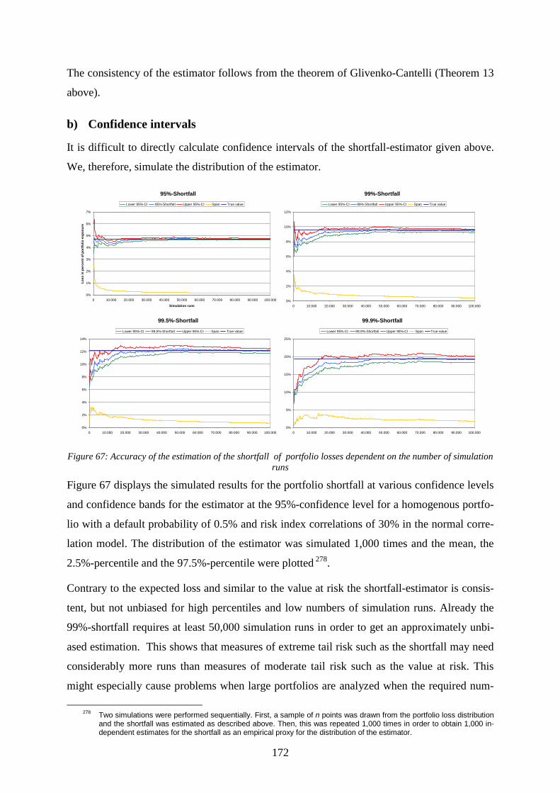
172

The consistency of the estimator follows from the theorem of Glivenko-Cantelli (Theorem 13

above).


It is difficult to directly calculate confidence intervals of the shortfall-estimator given above.

We, therefore, simulate the distribution of the estimator.

95%-Shortfall

0%

1%

2%

3%

4%

5%

6%

7%

0 10.000 20.000 30.000 40.000 50.000 60.000 70.000 80.000 90.000 100.000

Simulation runs

Loss

in p

erce

nt o

f por

tfolio

exp

osur

e

Lower 95%-CI 95%-Shortfall Upper 95%-CI Span True value

99%-Shortfall

0%

2%

4%

6%

8%

10%

12%

0 10.000 20.000 30.000 40.000 50.000 60.000 70.000 80.000 90.000 100.000

Lower 95%-CI 99%-Shortfall Upper 95%-CI Span True value

99.5%-Shortfall

0%

2%

4%

6%

8%

10%

12%

14%

0 10.000 20.000 30.000 40.000 50.000 60.000 70.000 80.000 90.000 100.000

Lower 95%-CI 99,5%-Shortfall Upper 95%-CI Span True value

99.9%-Shortfall

0%

5%

10%

15%

20%

25%

0 10.000 20.000 30.000 40.000 50.000 60.000 70.000 80.000 90.000 100.000

Lower 95%-CI 99,9%-Shortfall Upper 95%-CI Span True value

Figure 67: Accuracy of the estimation of the shortfall of portfolio losses dependent on the number of simulation runs

Figure 67 displays the simulated results for the portfolio shortfall at various confidence levels

and confidence bands for the estimator at the 95%-confidence level for a homogenous portfo-

lio with a default probability of 0.5% and risk index correlations of 30% in the normal corre-

lation model. The distribution of the estimator was simulated 1,000 times and the mean, the

2.5%-percentile and the 97.5%-percentile were plotted 278.

Contrary to the expected loss and similar to the value at risk the shortfall-estimator is consis-

tent, but not unbiased for high percentiles and low numbers of simulation runs. Already the

99%-shortfall requires at least 50,000 simulation runs in order to get an approximately unbi-

ased estimation. This shows that measures of extreme tail risk such as the shortfall may need

considerably more runs than measures of moderate tail risk such as the value at risk. This

might especially cause problems when large portfolios are analyzed when the required num-

278 Two simulations were performed sequentially. First, a sample of n points was drawn from the portfolio loss distribution and the shortfall was estimated as described above. Then, this was repeated 1,000 times in order to obtain 1,000 in-dependent estimates for the shortfall as an empirical proxy for the distribution of the estimator.

173

ber of simulation runs cannot be performed within an acceptable amount of time. It is left for

future research to develop more efficient estimators of shortfall risk that overcome these diffi-

culties.

D. Risk analysis and risk management

Having quantified portfolio risk under several respects on the aggregate level for the portfolio

as a whole, for a proactive risk management, i.e. for a risk management that methodically

seeks opportunities and pitfalls and acts early, it is essential

• to understand and visualize portfolio structures,

• to compare portfolio components as to their contribution of risk and positive occasion

to the portfolio,

• and to receive some hints by what actions portfolio risk can be reduced and how its

composition from the risk management’s point of view and its profitability can be im-

proved.

In the subsequent sections, we will describe the concepts of marginal risks and expected risk

adjusted returns. We will also show how they can be combined with the portfolio’s exposure

distribution to construct further risk measures, to define various types of limits, and to display

the results in a ‘risk management cockpit’. A risk management cockpit is a set of graphical

visualizations that summarize the results and outline the portfolio components that need the

risk manager’s immediate attention. Finally, we state an algorithm how the portfolio shortfall

can be minimized conditional to the portfolio’s expected risk adjusted return.

To illustrate the notion of risk contributions and the analysis and risk management techniques,

we analyze successively an example portfolio in the whole section. The example portfolio is

almost homogenous279 in the normal correlation model. It comprises clients in ten rating

grades who have the following default probabilities and exposures:

RatingI II III IV V VI VII VIII IX X

Default Probability 0,03% 0,05% 0,09% 0,30% 0,50% 1,20% 3,10% 6,00% 7,50% 10,00%

Unsecured Exposure 24 5 12 17 28 18 11 19 7 5

Table 11: Definition of the example: default probabilities and exposures

279 See above section II.A.2.a)(4).

174

Losses given default are set to 100%. Risk index correlations are assumed to equal 20%. For

simplicity, but without real loss in generality, it is assumed that the only type of financial

products consists in one year zero bonds280. The rating grades are defined as the portfolio seg-

ments of interest.

Portfolio Loss Distribution

6,21

% =

95%

-VaR

10,3

5% =

99%

-VaR

12,2

2% =

99.

5%-V

aR

16,8

2% =

99.

9%-V

aR

23,7

0% =

99.

99%

-VaR 30

,69%

= 9

9.99

9%-V

aR

0%

8%

16%

24%

32%

40%

0,000010,00010,0010,010,11

Confidence Level

Loss

in p

erce

nt o

f por

tfolio

val

ue

0 90% 99,9%99% 99,99% 99,999%

Figure 68: Loss distribution of the example portfolio

1. Marginal risks

For any risk measure, a portfolio segment’s marginal risk is defined as its contribution to the

total value of the risk measure for the entire portfolio. Thus, for instance, a segment’s mar-

ginal 99%-value at risk is calculated as follows:

• Calculate the 99%-value at risk V1 for the entire portfolio.

• Remove the segment from the portfolio.

• Recalculate the 99%-value at risk V2 for the remaining portfolio.

• The segment’s marginal 99%-value at risk is then the difference V1 - V2 of both values.

a) Marginal risks conditional to default

The simplest concept of risk contributions are marginal risks conditional to default of a speci-

fied portfolio segment. In this case, the segment’s risk contribution is identical with its (unse-

cured281) exposure, i.e. its absolute loss given default.

280 The types of financial products that are traded by a bank affects only the methodology how the fair risk premium is to

be calculated. It does not affect the calculation of expected risk adjusted returns and the risk management techniques. 281 In many models it is assumed that an exposure’s secured part cannot be lost, even in case of default of the creditor. In

practice, however, it frequently occurs that the value of securities turns out to be much lower than expected. In conse-

175

Exposure distribution and exposure limits

24

5

12

17

28

18

11

19

7

5

0

5

10

15

20

25

30

I II III IV V VI VII VIII IX X

Segment

Expo

sure

Exposure limit

worse

better

Figure 69: Exposure distribution and exposure limits

Figure 69 shows the exposure distribution of the example portfolio and indicates a possible

exposure limit. Note that since a segment’s exposure is its marginal risk conditional to de-

fault, the results are independent of clients’ default probabilities. Exposure limits are, there-

fore, equivalent to the statement

“I don’t want to lose more than X € if one segment defaults.”

In the example, segment 1 and segment 5 exceed the set limit. As a consequence, the risk

manager would have to inform the bank’s management that exposures in both segments

should be reduced.

b) Marginal risks prior to default

Marginal risks prior to default or simply marginal risks have many more facets than mere ex-

posures. It is important to note that a segment’s marginal risk does not only depend upon

creditworthiness and exposure of the segment itself, but very importantly also on the other

components of the portfolio if the portfolio standard deviation, the value at risk or the short-

fall are used as basic risk measures in the analysis. The concept of marginal risk is, therefore,

suited to analyze the risk structure of a portfolio and to localize areas of high risk concentra-

tions and others that are better diversified in the portfolio.

quence, many banks account for the entire exposure as a client’s or a segment’s marginal risk conditional to default. For the same reason, the loss given default on the unsecured exposure usually is set to 100% in this analysis.

176

Risk and exposure contributions relative to respective total

0,60

%

0,20

%

0,80

% 3,17

%

7,99

% 10,3

7% 12,9

8%

35,6

2%

15,2

2%

13,0

6%

16,4

4%

3,42

%

8,22

%

11,6

4%

19,1

8%

12,3

3%

7,53

%

13,0

1%

4,79

%

3,42

%

0%

5%

10%

15%

20%

25%

30%

35%

40%


Segment (= rating grade)

Con

trib

utio

n re

lativ

e to

tota

l ris

k

99%-marginal Value at Risk Exposure

Figure 70: Risk and exposure concentrations

Figure 70 compares segments’ concentrations282 of exposures and of the 99%-marginal values

at risk. It is evident that risk and exposure concentration greatly differ for almost all segments.

Risk concentrations are much lower than exposure concentrations particularly for segments

with high creditworthiness283. For instance, segment 1 contributed 16.44% to portfolio expo-

sure and even exceeded an exposure limit, but only 0.6% to portfolio risk due to its extremely

low probability of default. The opposite is true for segments with low creditworthiness. Seg-

ment 8 represents 13.01% of portfolio exposure, but not less than 35.62% of total portfolio

risk. In other words, approximately 1/8th of portfolio exposure may stand for 1/3rd of portfolio

risk.

282 In this analysis it is assumed that the set of all segments is a partition of the total portfolio. A segment’s risk concentra-

tions in the portfolio is then defined as its marginal risk divided by the sum of all marginal risks. Exposure concentra-tions are defined respectively. Note that the concept of risk concentrations can also be used to distribute economic capital to portfolio components. This is particularly so because they sum up to 1.

283 Segments are identical with rating grades in the example.

177

Risk contributions relative to total risk and concentration limits

0,60

%

0,20

%

0,80

% 3,17

%

7,99

% 10,3

7% 12,9

8%

35,6

2%

15,2

2%

13,0

6%

0%

5%

10%

15%

20%

25%

30%

35%

40%

I II III IV V VI VII VIII IX XSegment

Ris

k co

ntrib

utio

n re

lativ

e to

tota

l ris

k

99%-marginal Value at Risk

Concentration limit

worse

better

Figure 71: Risk concentrations and concentration limits

Similar to losses given default also risk concentrations can be limited. Here, the limit corre-

sponds to the conviction

“I don’t want to concentrate more than X% of the total portfolio risk in one segment.”

Note that segment 1 and 5, that surpassed the exposure limit, are both far away from going

beyond the concentration limit. On the other hand, exposure should be reduced in segment 8

in favor of other segments.

Complementary to risk concentrations, absolute marginal risks can be compared and limited

(Figure 72).

Absolute risk contributions

0,09

0,03 0,

12

0,48

1,20

1,56

1,96

5,37

2,29

1,97

0

1

2

3

4

5

6


Con

trib

utio

n re

lativ

e to

tota

l ris

k


risk limit

worse

better

Figure 72: Absolute risk contributions and risk limits

178

Absolute risk contributions may, however, increase with the size of the portfolio. This is par-

ticularly true for the portfolio standard deviation as basic risk measure, which monotonously

increases in portfolio exposure if default correlations are positive284. Less systematically,

similar effects can occur if other risk measures are used. Limits to risk contributions are,

therefore, much more difficult to interpret and have to be adjusted from time to time if the

size of the portfolio changes.

c) Combinations of exposure and marginal risk

So far only simple risk measures were considered. However, sometimes it can be helpful to

combine risk measures to get a more complete picture of the situation.

Risk versus exposure + contribution to total risk 99%-marginal value at risk by segment

0,6%

0,2%

0,8%

3,2%

8,0%

13,0%

13,0%

35,6%

15,2%

13,1%

0

5

10

15

20

25

30

0% 10% 20% 30% 40%

Risk per exposure unit

Expo

sure


low impact - low risk - area

HIGH impact - HIGH risk - area

low impact - HIGH risk - area

HIGH impact - low risk - area

contribution to total risk

risk limit

exposure limit

Figure 73: Risk versus exposure and risk concentration

Figure 73 displays three quantities at a time: on the axies the segments’ absolute exposure

versus their marginal risk contribution per exposure unit. The size of the bubbles indicates the

risk concentration in each segment.

The segments of interest for the risk manager can be identified in several ways. Firstly, by the

size of the bubbles. This analysis boils down to the same result as Figure 71.

Secondly, segments can be compared by absolute exposure and exposure limits can be ap-

plied. We see even more clearly than in Figure 69 that segment 1 and 5 are well above the set

limit.

284 Positive default correlations are the standard case in all of the quoted portfolio models.

179

Thirdly, segments can be contrasted by risk per exposure unit. Particularly, risky segments

can be ruled out by the definition of risk limits. In our example, segment 10 clearly is in ex-

cess of the outlined limit.

Fourthly, all three features can be evaluated simultaneously. For this the chart can be divided

in four quadrants. The lower left quadrant contains the small exposures that are subject to

relatively low risks. Segments in this sector are inconspicuous. Moreover, limits and credit

production could even be increased in the particular segments285.

The upper left and the lower right quadrants correspond to the yellow traffic light. They com-

prise of respectively large exposures of relatively low risks and small, but risky exposures.

Segments in these areas do not need urgent action, but they need close attention. This is more

immediate if a segment represents a large risk-concentration in the portfolio. Segments 6 and

9 certainly need to be watched more carefully than segments 1 or 4. In this context, the report-

ing of risk-concentrations does not only supply an information that is valuable in itself, but it

helps to prioritize the risk manager’s monitoring activities and the establishment of both a

watch list and an early warning system. In practice, the detection of imminent problems of

segments in this area can lead to some action such as the reduction of individual limits, the

hint to the bank’s sales unit not to produce more exposure in the respective segments or the

sale of parts of a segment’s risk with the help of a credit derivative.

The upper right quadrant contains the explosives in the portfolio. It comprises the large and

risky exposures where serious losses for the bank can be expected at any moment. Segments

in this area require immediate action such as the instant reduction of exposure limits prevent-

ing the production of new credits in the respective areas, the selling of risk via credit deriva-

tives and the obligation of the affected clients to supply additional securities or guaranties.

d) Expected risk adjusted returns

Limit management in the sense of limit supervision is reactive by definition. A methodical

risk analysis and a functioning early warning system as discussed in the previous section are

already much more proactive because they frequently indicate which limits should be rede-

fined and supply background information that has a certain relevance for the management of a

bank’s credit production.

In order to establish a full-fledged proactive risk management that systematically seeks oppor-

tunities and tries to increase a bank’s profitability at the same time as to improve the portfolio

285 In practice, the size of the limits may vary with the segment, of course, although not symbolized in our example.

180

structure it is necessary to also include the segments’ expected risk adjusted return into the

examination.

A contract’s expected risk adjusted return is defined as the contract’s market interest rate less

its fair risk premium286 for a target return on equity that is equal to the long term risk free rate.

If the return on equity equals the long term risk free rate, the credit’s expected risk adjusted

return on economic capital287 can be zero and the long term risk free rate is still earned on the

economic capital, i.e. the credit has a net profitability of zero. A segment’s risk adjusted re-

turn then simply is the average of the risk adjusted returns of all contracts belonging to the

segment weighted with each contract’s contribution to the segment’s total exposure.

Refinance Rate Long Term Risk Free Rate Target Return on Equity4,75% 8,50% 25%

RatingI II III IV V VI VII VIII IX X

Market Rates 5,00% 5,10% 5,25% 5,90% 6,35% 7,80% 11,25% 12,00% 12,40% 12,60%

Table 12: Definition of the example: relevant interest rates

Table 12 states the values of the relevant interest rates for the analysis in our example. Market

rates refer to a one-year zero bond with a counterparty having rating 1-10. Our bank can lend

one-year-money at the refinance rate. Equity is invested at the long term risk free rate.

Granted loans are intended to earn the difference to the target return on equity288.

Expected risk adjusted return on economic capital

58,29%

50,10%

40,60%

29,67%

24,96%

20,47%17,70%

2,00%

-2,57%

-9,62%

-20%

-10%

0%

10%

20%

30%

40%

50%

60%

70%


Expe

cted

risk

adj

uste

d re

turn

on

capi

tal


RAROC limit

better

worse

stopp loss limit

destruction limit

Figure 74: Expected risk adjusted return on economic capital

286 For the calculation of the fair risk premium see above section I.E.1. 287 The economic capital is defined as the capital that is supplied by the bank to cover the contract’s risk. We suppose

that the 99%-marginal value at risk is used to calculate economic capital instead of regulatory approaches. 288 See section I.E.1 above for more details on the role of the interest rates and all calculations. Particularly, we assume

that on the one hand the whole credit volume is refinanced by leverage capital and that on the other hand the entire equity is invested at the long term risk free rate so that lent out money only has to earn the difference between target return on equity and the long term risk free rate.

181

Figure 74 shows the results for the expected risk adjusted return on economic capital

(RAROC) for the example portfolio in the various segments and three types of limits. The

RAROC limit marks the level of RAROC where the bank meets the target return on equity

exactly. The stop loss limit stands for a RAROC of zero. Finally, the destruction limit is equal

to the negative long term risk free rate.

As a consequence, four different areas can be distinguished in this chart. Firstly, a portfolio

segment with a RAROC above the RAROC limit earns a higher return on equity than the in-

tended target return. These segments are most profitable and, therefore, of particular interest

for a proactive risk management. In our example, segment 1 to 7 belong to this group.

Secondly, segments with a RAROC between the RAROC limit and the stop loss limit still

increase the bank’s return on equity above the long term risk free rate, although their profit-

ability is too low to meet the target return on equity. It is still better to invest in segments in

this area than to stop granting credits at all if counterparties in the first group are not available

as creditors. Segment 8 falls in this area in the example.

Thirdly, below the stop loss limit, but above the destruction limit the RAROC is negative im-

plying that the bank’s return on equity is reduced below the long term risk free rate, but still

remains positive. Since a safe profit is lost it is not worthwhile investing in segments in this

area. Segment 9 embodies this group in the example.

Fourthly, below the destruction limit, a segment’s RAROC is so low that it fully absorbs the

payoff of the investment of equity at the long term risk free rate. In this area, the bank expects

to lose money from business with the respective segments, segment 10 in the example, and

should immediately stop producing new contracts.

In the example, additional business with segment 9 and especially segment 10 is not desirable.

Instead, credit production should be directed to segment 1 to 7 and, perhaps, segment 8 if nec-

essary.

Once again, the expected risk adjusted return on capital is not the whole story since the size of

accepted risk necessary to produce a certain RAROC may vary significantly between portfo-

lio segments. It is, therefore, valuable to plot the expected risk adjusted return per exposure

unit against the accepted risk per exposure unit (see Figure 75).

182

RAROC versus risk + contribution to total risk 99%-marginal value at risk by segment

0,6%

0,2%

0,8%

8,0%13,0%

13,0%

35,6%

15,2%

13,1%

3,2%

-30%

-20%

-10%

0%

10%

20%

30%

40%

50%

60%

70%

0% 10% 20% 30% 40%

Risk per exposure unit

RA

RO

C p

er e

xpos

ure

unit


contribution to total risk

risk limit

RAROC limit

stopp loss limit

destruction limit

constant return / risk ratio on lines

worse

better

Figure 75: Accepted risk versus expected risk adjusted return per exposure unit and contribution to total risk

In the exhibit, RAROC, risk and risk concentration are combined showing that segment 10

misses several limits at a time. Conversely, segments 1 to 5 appear particularly favorable from

the point of view of satisfying all three criteria simultaneously. Segments 6 and 7 are still

above the RAROC limit, but carry a medium sized risk per exposure unit and already repre-

sent considerable risk concentrations in the portfolio.

e) Summary

It has become clear from the discussion above that credit portfolio analysis is a multidimen-

sional task. Being unobtrusive or even positive from one point of view, a segment may be less

or even undesirable from another.

In the example, segment 1, having the highest credit worthiness, has the most favorable

RAROC, carries very little risk per exposure unit and represents only a small risk concentra-

tion in the portfolio so that one would want to enlarge business in that area. Unfortunately,

segment 1 already exceeds the exposure limit, though, so that additional credit production is

impossible here. Although less pronounced, the same argument holds true for segment 5.

On the other hand, segments 8 to 10 are so risky and so little profitable that credit granting

should be avoided in this area. This is especially so as a result of the poor RAROC of seg-

ments 9 and 10, the additionally enormous risk concentration in segment 8 and the surpassing

of the risk limit by segment 10.

This analysis leads to the following actions:

• Stop credit production in segments 1, 5, 8, 9, 10.

183

• Reduce risk in segments 8 and 10.

• Increase credit production in segments 2, 3, 4, 6, and 7, particularly in segments 2, 3,

and 4, less so in segments 6 and 7.

2. Credit derivatives

It is a typical problem for a credit portfolio manager that there are portfolio segments where

risk is undesirably strongly concentrated or surpasses risk limits so that he would like to re-

duce risk in the respective areas to rebalance the portfolio. In this situation, credit derivatives

can be applied. ‘Credit derivative’ is an umbrella term for all kinds of insurance contracts

against losses from credit risks. They enable a bank to transfer the credit risk from a specific

contract or a portfolio of contracts to another bank or a group of banks.

We don’t want to discuss the design and application of credit derivatives in detail. We rather

want to state two essential prerequisites for the successful appliance of credit derivatives in

the interbank risk trade.

Firstly, in order to sell the risk of the right portfolio components, a risk manager has to have

the necessary implements to quantitatively analyze the portfolio he is responsible for.

Secondly and more importantly, the quantitative and qualitative structure of the sub-portfolio

whose risk is to be transferred has to be transparent for all parties that participate in the credit

derivative so that the contract can be objectively valued. This is particularly true for the as-

sessment of default probabilities of counterparties in the sub-portfolio. The risk selling bank

has to make its internal rating results accessible for the risk taking bank and also has to prove

that its rating methodology is conceptually sound so that an objective benchmark price for the

derivative can be calculated. This transparence requirement is a central side condition when a

new internal rating scheme is implemented.

3. Portfolio optimization

A complementary approach to improve portfolio quality is algorithmic portfolio optimization

under certain constraints such as non-negativity of exposures, the size of expected returns or

others. This was long an unsolved problem because the standard approach of minimizing port-

folio variance under side-constraints was difficult to apply to credit portfolios due to the lack

of interpretability of portfolio variance (or standard deviation). However, in their 1999 semi-

184

nal paper Stanislav Uryasev and Tyrell Rockafellar289 proposed a methodology to minimize

portfolio shortfall290 under the respective side-constraints.

a) Optimization approach

Indicate clients (or portfolio segments of interest291) by i for ni ...,,1= . Let

( ) nnXXX 01,..., ≥⊂Ω∈= R be the vector of clients’ exposures in the portfolio chosen out of a

certain subset n0≥⊂Ω R . In the sense of the optimization problem, X is a decision vector re-

flecting the composition of the credit portfolio. Let ( ) nnYYY R∈= ,...,1 be a random vector

that stands for the uncertainties of the future value of the exposures. For ease of exposition we

assume in the following that the distribution of Y is continuous with density ( )Yp . In prac-

tice, the distribution of Y need not be known analytically, but is being simulated in accor-

dance with the portfolio model used292. Let ( ) R∈YXf , be the portfolio loss associated with

the exposure vector X and the random ‘creditworthiness’ vector Y. For given X, the distribu-

tion of ( )YXf , is the portfolio loss distribution.

Let further

( ) ( ) ( )( )∫≤

=≤=Ψα

ααYXf

dYYpYXfPX,

,:,

be the probability that ( )YXf , does not exceed a given threshold α.

For a given confidence level ( )1,0∈β the β-VaR and the β-shortfall are

( ) ( ) βααβ ≥Ψ∈= ,:min XXVaR R

and

( ) ( ) ( )( ) ( )

∫>−

=XVaRYXf

dYYpYXfXSβ

ββ,

,1

1 .

289 Rockafellar and Uryasev 1999. 290 Minimization of portfolio shortfall is not equivalent to minimization of portfolio value at risk. The shortfall always domi-

nates the respective value at risk. 291 In practice, it may be difficult to do a portfolio optimization at the client level because single clients’ exposures usually

cannot be modified easily without the respective client’s agreement. For this reason, it is rather more practicable to consider portfolio segments at an intermediate level of aggregation in the portfolio where exposures can be more freely adapted.

292 Note in particular, that the methodology suggested by Rockafellar and Uryasev is independent of the actual portfolio model that is used by a financial institution to assess portfolio risk. The only place where the portfolio model enters in is the simulation of clients’ future creditworthiness.

185

The key to the optimization approach of Rockafellar and Uryasev is the characterization of

optimal shortfall and the corresponding value at risk in terms of the function βF defined as

( ) ( )[ ] ( )∫∈

+−−

+=nY

dYYpYXfXFR

αβ

ααβ ,1

1, .

The relationship between optimal shortfall, corresponding value at risk and the function βF is

captured in the following

Theorem 15 (Rockafellar and Uryasev 1999):

Minimizing the β-shortfall of the loss associated with X over all Ω∈X is equivalent to

minimizing ( )αβ ,XF over all ( ) R×Ω∈α,X , in the sense that

( )( )

( )αβαβ ,minmin,

XFXSXX R×Ω∈Ω∈

= .

A pair ( )** ,αX achieves the second minimum if and only if *X achieves the first minimum

and ( )** XVaRβα = .

According to the theorem, it is sufficient to do the minimization of the β-shortfall with the

function βF that does not contain the β-VaR, which often is mathematically troublesome to

handle, instead of using the β-shortfall directly. The theorem also states that the value at risk

corresponding to the optimal β-shortfall is automatically given as one of the calculation re-

sults, quasi as a byproduct of the optimization.

In practice, the distribution of Y in βF can be approximated by a sampled empirical distribu-

tion due to the theorem of Glivenko-Cantelli. With simulation results mYY ,...,1 the approxima-

tion βF~ of βF can be defined as

( ) ( ) ( )[ ]∑=

+−−

+=m

jjYXf

mXF

1,

11,~ αβ

ααβ .

b) A portfolio optimization

As an example, we consider a heterogeneous portfolio of 10,000 clients293 in n = 20 segments

with a total portfolio exposure of € 1,000 in the normal correlation model294. Risk index cor-

293 Individual default probabilities, exposures and segment adherence were assigned randomly.

186

relations were set to 30%. The portfolio loss distribution was sampled m = 2,000 times295.

Exposures and losses were aggregated per segment in each simulation run so that the optimi-

zation can be performed at the segment level296. The coefficients of the random vector

( ) nnjjj YYY R∈= ,...,1 signify which fraction of the portfolio exposure in the respective segment

was lost in simulation run j for j = 1, …, m. The portfolio loss function f then simply is

( ) YXYXf t=,

so that the optimization problem can be stated as

( ) ( ) [ ]∑=

+

∈Ω∈∈Ω∈−

−+=

m

jj

t

XXYX

mXF

1,, 11min,~min αβ

αααβα RR

.

With ( )mUUU ,...,1= this is the same as

( ) ∑=∈∈∈ −

+m

jjUX

Ummn

1,, 11minβ

αα RRR

subject to

0,

,

≥

−≥Ω∈

j

tj

UYXU

Xα

for j = 1, …, m, so that the task is reduced to a linear optimization problem297.

The feasibility set n0≥⊂Ω R was specified as a linear return-constraint298

∑=⋅≥

n

ii

t XXr1

θ

where ( ) nnrrr R∈= ,...,1 is the vector of expected returns per exposure unit in each segment

for fixed values of 0>θ and the trivial constraint

0≥iX

294 The normal correlation model was used as a pure default model so that rating migrations other than to default were ig-nored.

295 The optimization was performed with an own implementation of the simplex algorithm. It turned out that the algorithm could not handle problems with more than about 2,000 constraints, thus, limiting the number of simulation runs (see below). 2,000 runs are, however, too few to precisely forecast the 95%-shortfall. Optimization results are, therefore, rather illustrative in nature. A serious implementation would need a high-end linear solver such as IBM-OSL or CPLEX.

296 We suppose that the composition of the segments remains unchanged by the optimization. 297 Note that the simplex algorithm assumes non-negativity of all variables so that the number of non-trivial constraints is

approximately equal to the number of simulation runs. 298 Other possible linear constraints are exposure limits or exposure concentration limits. Risk or risk concentration limits

usually are non-linear in nature.

187

for i = 1, …, n.

Marginal VaR before and after optimisation

0%

10%

20%

30%

40%

50%

60%

0 20 40 60 80 100 120

Marginal exposure

Mar

gina

l VaR

in p

erce

nt o

f mar

gina

l exp

osur

eMarginal VaR before optimisation Marginal VaR after optimisation

Figure 76: Marginal VaR before and after optimization

Figure 76 shows the segments’ marginal values at risk before and after optimization of the

95%-portfolio shortfall. It is particularly striking that after the optimization the number of

small exposures with high marginal risks has decreased substantially. Note moreover that one

segment has an exposure of zero after the optimization and has completely dropped out of the

portfolio.

VaR and shortfall efficient frontiers

8,0%

6,5%

5,5%

5,0%

4,7%

4,6%

4,5%

4,6%

5,0%

5,5%

6,2%

7,0%

8,4%

10,0%

12%

14%

17%

20%

15,0%

11,3%

9,4%

8,2%

7,6%

7,5%

7,4%

7,5%

8,0%

8,6%

9,8%

11,6%

14,0%

17,2%

21,2%

26,0%

31,0%

35,6%

11,3% 20,8%

0%

1%

2%

3%

4%

5%

6%

7%

0% 5% 10% 15% 20% 25% 30% 35% 40%

Risk in percent of portfolio exposure

Expe

cted

retu

rn

VaR efficient frontier shortfall efficient frontier VaR before optimisationshortfall before optimisation original portfolio return

Figure 77: VaR and shortfall efficient frontiers

188

Figure 77 illustrates the efficient frontiers299 of the example portfolio for different values of

the minimum expected return θ . It turns out that the optimization had a remarkable effect on

the portfolio shortfall and also on the portfolio value at risk by reducing risk by more than

half in both cases. Overall, the optimization greatly improved portfolio quality both from the

point of view of portfolio structure and total portfolio risk.

Conclusion

The discussion has shown that credit risk modeling and management is a complex task where

many different aspects play an important role and where many errors can be committed. The

analysis has identified some of these errors, particularly in the estimation of default probabili-

ties and the concepts of dependence among clients. Most importantly, the thesis proposes so-

lutions for some of the deficiencies of current risk models.

Moreover, the entire risk management process has been assessed and methods for portfolio

analysis and management have been described in detail. We are convinced that some of our

results can help financial institutions to avoid some of the pitfalls of credit risk modeling and

management and to improve the quality of their risk management methods and in turn the

credit risk quality of their portfolios.

299 Only the portfolio shortfall was optimized. The values for the value at risk just correspond to the respective shortfalls

and may not be optimal for a value at risk criterion. Experiments with various portfolios also showed that the value at risk efficient frontier is not necessarily convex. Moreover, we also found examples where the portfolio value at risk effi-cient frontier did not even fall into a part that was monotonously decreasing and another that was increasing in the ex-pected return. In practice, the VaR-efficient frontier can take a great variety of shapes.

189

Literature

Altman, Edward I. and V.M. Kishore, 1996, “Almost everything you wanted to know about

recoveries and defaulted bonds,” Financial Analysts Journal, pp. 57-63

Artzner, Phillippe and Freddy Delbaen and Jean-Marc Eber and David Heath, 1998, “Coher-

ent measures of risk,” Working Paper Strassburg University

Bär, Tobias, 2000, “Predicting business failure rates: empirical macroeconomic models for 16

German industries,” Working Paper, McKinsey & Co.

Barndorff-Nielsen, Ole E. and O. Halgreen, 1977, “Infinite divisibility of the hyperbolic and

generalized inverse Gaussian distributions”, Zeitschrift für Wahrscheinlichkeitstheorie und

verwandte Gebiete 38, pp. 309-312

Basel Committee on Banking Supervision, 2001, “Potential modification to the Committee’s

proposals,” http://www.bis.org

Bassi, Franco and Paul Embrechts and Maria Kafetzaki, 1998, “Risk management and quan-

tile estimation,” in: ‘A practical guite to heavy tails: statictical techniques and applications,’

edited by Robert J. Adler, Raisa E. Feldman, Murad S. Taqqu, p. 110-130.

BIS, 1996, “Amendment to the capital accord to incorporate market risks”, Basle Committee

on Banking Supervision, Bank for International Settlement, Basle

Black, Fisher and Myron Scholes, 1973, “The pricing of options and corporate liabilities,”

Journal of Political Economy, pp. 637-659

Caouette, John B. and Edward I. Altman and Paul Narayanan, 1998, “Managing credit risk:

the next great financial challenge,” John Wiley & Sons.

Carty, Lea and Dana Lieberman, 1996, “Corporate bond defaults and default rates 1938-

1995,” Moody’s Investors Service Global Credit Research

Credit Suisse Financial Products (1996), “Credit Risk +, a credit risk management frame-

work,” Working Paper

Creditreform, 2002, „Insolvenzen in Europa 2001 / 2002“, Creditreform Research Report

Crosby, Peter J., 1997, “Modeling default risk,” Working Paper, KMV Corporation,

http://www.kmv.com

190

Crouhy, Michael; Dan Galai and Robert Mark, 2000, „A comparative analysis of current

credit risk models,“ Journal of Banking & Finance 24, pp. 59-117

Deutsche Bundesbank, 2001, “Bankbilanzen, Bankenwettbewerb und geldpolitische Trans-

mission,” Monatsbericht September 2001, pp. 51-70

Eberlein, Ernst and Karsten Prause, 1998, “The generalized hyperbolic model: financial de-

rivatives and risk measures,” Working paper Nr. 56, University of Freiburg

Embrechts, Paul and Alexander McNeil and Daniel Straumann, 1999, “Correlation and de-

pendence in risk management: properties and pitfalls,” Working paper, ETH Zurich

Embrechts, Paul and Filip Lindskog and Alexander McNeil, 2001, “Modelling dependence

with copulas and applications to risk management,” Working Paper, ETH Zürich

Fang, Kai-Tai and Samuel Kotz and Kai-Wang Ng, 1989, “Symmetric multivariate and re-

lated distributions,” Monographs on Statistics and Applied Probability 36

Federal Reserve System Task Force Report, 1998, “ Credit risk models at major US banking

institutions: Current state of the art and implications for assessments of capital adequacy,”

Working Paper, US Federal Reserve System, Washington, DC

Finger, Christopher C., 1999, “Conditional approaches for Credit Metrics portfolio distribu-

tions,” Credit Metrics Monitor April 1999, pp. 14-33

Frey, Rüdiger and Alexander McNeil, 2001, “Modelling dependent defaults,” Working Paper,

Swiss Banking Institute and ETH Zurich

Frey, Rüdiger and Alexander McNeil and Mark Nyfeler, 2001, “Modelling dependent de-

faults: asset correlations are not enough!,” Working paper, ETH Zurich

Gersbach, Hans and Uwe Wehrspohn, 2001, “Die Risikogewichte der IRB-Ansätze: Basel II

und schlanke Alternativen,” RiskNEWS Special Edition 11.2001, pp. 3-32

Gersbach, Hans and Uwe Wehrspohn, 2001, “Lean IRB approaches and transition design: the

Basel II proposal,“ Working Paper, Heidelberg University and Computer Sciences Corpora-

tion

Gesetz über das Kreditwesen – KWG, 1998, In der Neufassung der Bekanntmachung vom 9.

September 1998 (BGBl. I S. 2776) zuletzt geändert durch Art. 1 des Gesetzes zur Änderung

des Einführungsgesetzes zur Insolvenzordnung und anderer Gesetze (EGInsOÄndG) vom 19.

Dezember 1998 (BGBl. I S. 3836).

191

Gordy, Michael, 2000, “A comparative anatomy of credit risk models,” Journal of Banking

and Finance 24, pp. 119-149

Grundsatz 1 über die Eigenmittel der Institute – Grundsatz 1, Bekanntmachung Nr. 1/69 vom

20. Januar 1969 (BAnz. Nr. 17 vom 25. Januar 1969), zuletzt geändert durch die Bekannt-

machung vom 29. Oktober 1997 (BAnz. S. 13555), Deutsche Bundesbank

Gupton, Greg M., Christopher C. Finger, Mickey Bhatia, 1997, “Credit Metrics – Technical

Document,” Working Paper, JP Morgan

Jarrow, Robert A. and Stuart M. Turnbull and D. Lando, 1997b, “A Markov model for the

term structure of credit risk spreads,” Review of Financial Studies 10, pp. 481-523

Jarrow, Robert A. and Stuart M. Turnbull, 1995, “Pricing derivatives on financial securities

subject to credit risk,” Journal of Finance 50, pp. 53-85

Jarrow, Robert A. and Stuart M. Turnbull, 1997a, “An integrated approach to the hedging and

pricing of eurodollar derivatives,” Journal of Risk and Insurance 64, pp. 271-299

Jarrow, Robert, 2000, “Default parameter estimation using market prices,” Working Paper

Jarrow, Robert A. and Stuart M. Turnbull, 2000, “The intersection of market and credit risk,”

Journal of Banking & Finance 24, pp. 271-299

Kealhofer, Stephen, 1993, “Portfolio management of default risk,” Working paper, KMV

Corporation, http://www.kmv.com

Kealhofer, Stephen, Sherry Kwok and Wenglong Weng, 1998, “Uses and abuses of bond de-

fault rates,” Working Paper, KMV Corporation, http://www.kmv.com

Kim, Jongwoo, 1999, “A way to condition the transition matrix on wind,” Working Paper,

Riskmetrics Group

Koyluoglu, H. Ugur and Andrew Hickman, 1998, “A generalized framework for credit risk

portfolio models,” Working paper, Oliver, Wyman & Company and Credit Suisse Financial

Products

Lehment, Harmen and Christoper Blevins and Espen Sjøvoll, 1997, “Gesamtwirtschaftliche

Bestimmungsgründe der Insolvenzentwicklung in Deutschland,” Institut für Weltwirtschaft an

der Universität Kiel, Kieler Arbeitspapier Nr. 842

192

Lipponer, Alexander, 2000, “Kreditportfoliomanagement: Die Bedeutung von Korrelationen

für die Bewertung von Kreditausfallrisiken,“ Dissertation Universität Heidelberg

Maddala, G.S., 1983, „Limited-dependent and qualitative variables in econometrics,” Econo-

metric Society monograps in quantitative econometrics 3, Cambridge University Press

McKinsey & Company, 1999, “Credit Portfolio View,” Technische Dokumentation

Merton, Robert C., 1974, “On the pricing of corporate debt: the risk structure of interest

rates,” Journal of Finance 39, pp. 449-470

Moody’s Investor’s Service, 1997, “Corporate bond defaults and default rates,” Moody’s Spe-

cial Reports

Moody’s Investor’s Service, 2000, “Ratings performance 2000,” Moody’s Special Reports

Nelson, R. B., 1999, An introduction to copulas, Springer, New York

Nyfeler, Mark A., 2000, „Modelling dependencies in credit risk management,“ Diploma The-

sis, ETH Zurich

Øksendal, Bernt, 1998, “Stochastic differential equations: an introduction with applications,”

Springer-Verlag

Overbeck, Ludger and Gerhard Stahl, 1998, “Stochastische Methoden im Risikomanagement

von Kreditportfolios,” in: Andreas Oehler (ed.), “Credit Risk und Value-at-risk Alternativen,”

pp. 77-110, Schäffer-Poeschel, Stuttgart

Prause, Karsten, 1999, “The generalized hyperbolic model: estimation, financial derivatives,

and risk measures”, Dissertation University of Freiburg

Rockafellar, Tyrell and Stanislav Uryasev, 1999, “Optimisation of conditional value at risk,”

Working Paper University of Florida, http://www.ise.ufl.edu/uryasev

Schmidt, Rafael, 2002, “Tail dependence for elliptically contoured distributions,” Mathemati-

cal Methods of Operations Research, 55, pp. 301-327

Sellers, Martha; Oldrich Alfons Vasicek and Allen Levinson, 2000, “The KMV EDF credit

measure and probabilities of default,” Working Paper, KMV Corporation,

http://www.kmv.com

193

Sobehart, J.R. and S.C. Keenan, 1999, “Equity Market Value and Its Importance for Credit

Analysis; Facts and Fiction,” Research Report 2-7-7-99, Moody’s Risk Management Ser-

vices, http://www.moodys.com

Sobehart, Jorge R. and Roger M. Stein, 2000, “Moody’s public firm risk model: a hybrid ap-

proach to modeling short term default risk,” Working paper, Moody’s Investors Service,

http://www.moodys.com

Standard & Poor’s, 1991-1992, “Corporate bond defaults study,” Parts 1-3, Credit Week,

(September 15 and 16, and December 21, 1992

Standard & Poor’s, 1996, CreditWeek, (April 15, 1996), pp. 44-52

Standard and Poor’s, 2001, “Ratings performance 2000”

UBS (Union Bank of Switzerland), 2001, “Morning News, January 16, 2001”

Vasicek, Oldrich Alfons, 1984, “Credit Valuation,” Working Paper, KMV Corporation,

http://www.kmv.com

Vasicek, Oldrich Alfons, 1991, “Limiting loan loss probability distribution,” Working Paper,

KMV Corporation, http://www.kmv.com

Wehrspohn, Uwe and Hans Gersbach, 2001, “Die Risikogewichte der IRB-Ansätze: Basel II

und schlanke Alternativen,” RiskNEWS Special Edition 11.2001, pp. 3-32

Wehrspohn, Uwe, 2001, “Kreditrisikomodelle der nächsten Generation,” RiskNEWS 05.2001

Wehrspohn, Uwe, 2001, “Standardabweichung und Value at Risk als Maße für das Kreditrisi-

ko,” Die Bank, August 2001, pp. 582-588

Wehrspohn, Uwe, 2002, „Bestimmung von Ausfallwahrscheinlichkeiten – Das kanonische

Verfahren: Mittlere Ausfallhäufigkeiten,“ RiskNEWS 05.2002, pp. 7-18

Wehrspohn, Uwe, 2002, „Bestimmung von Ausfallwahrscheinlichkeiten – Marktdatenbasierte

Verfahren,“ RiskNEWS 07.2002

Wilson, Thomas C., 1997a, “Portfolio credit risk (I),” Risk 9, pp. 111-117

Wilson, Thomas C., 1997b, “Portfolio credit risk (II),” Risk 9, pp. 56-62

Wilson, Thomas C., 1997c, “Measuring and managing credit portfolio risk – Part 1: Model-

ling Systemic default risk,” The Journal of Lending and Credit Risk Management, reprint

194

Wilson, Thomas C., 1997d, “Measuring and managing credit portfolio risk – Part 1: Portfolio

loss distributions,” The Journal of Lending and Credit Risk Management, reprint

Wilson, Thomas C., 1998, “Portfolio credit risk,” FRBNY Economic Policy Review, reprint

195

Uwe Wehrspohn

is managing partner at the Center for Risk & Evaluation, a

consulting firm specializing in risk management strategies,

methodology and technology based in Heidelberg and Eppingen.

He also holds a research and teaching position at the University of

Heidelberg.

Uwe Wehrspohn has studied mathematics, economics and

theology in Montpellier, St. Andrews, Munich and Heidelberg. He then worked for several years as a

senior consultant at the Competence Center Controlling and Risk Management of Computer Sciences

Corporation in Europe.

CRE Center for Risk & Evaluation GmbH & Co. KG

Berwanger Straße 4 D-75031 Eppingen Germany Tel. +49 7262 20 56 12 Mobile +49 173 66 18 784 Fax + 49 7262 20 69 176 Email [email protected] www.risk-and-evaluation.com

Credit Risk Evaluation

Documents