Does Credit Risk Impact Liquidity Risk? Evidence from Credit ...

Munich Personal RePEc Archive

Does Credit Risk Impact Liquidity Risk?

Evidence from Credit Default Swap

Markets

Hertrich, Markus

September 2015

Online at https://mpra.ub.uni-muenchen.de/67837/

MPRA Paper No. 67837, posted 12 Nov 2015 14:21 UTC

1

Hertrich, International Journal of Applied Economics, 12(2), September 2015, 1-46

Does Credit Risk Impact Liquidity Risk?

Evidence from Credit Default Swap Markets

Markus Hertrich

Department of Finance, University of Basel, Peter Merian-Weg 6, CH-4052 Basel, Switzerland.

Email: [email protected]

Institute for Finance, University of Applied Sciences Northwestern Switzerland, Peter Merian-

Weg 86, CH-4052 Basel, Switzerland. Email: [email protected]

Abstract: During the recent financial crisis that erupted in mid-2007, credit default swap spreads

increased by several hundred basis points, accompanied by a liquidity shortage in the U.S.

financial sector. This period has both evidenced the importance that liquidity has for investors

and underlined the need to understand the linkages between credit markets and liquidity. This

paper sheds light on the dynamic interactions between credit and liquidity risk in the credit default

swap market. Contrary to the common belief that illiquidity leads to a credit risk deterioration in

financial markets, it is found that in a sample of German and Swiss companies, credit risk is more

likely to be weakly endogenous for liquidity risk than vice versa. The results suggest that a

negative credit shock typically leads to a subsequent liquidity shortage in the credit default swap

market, in the spirit of, for instance, the liquidity spiral posited by Brunnermaier (2009), and

extends our knowledge about how credit markets work, as it helps to explain the amplification

mechanisms that severely aggravated the recent crisis and also indicates which macro-prudential

policies would be suitable for preventing a similar financial crisis in the future.

Keywords: financial crisis, credit default swap, credit risk, liquidity risk, endogeneity, macro-

prudential policy

JEL classifications: E37, E61, G14, G32, G38

1. Introduction

The recent financial crisis that erupted in mid-2007, less than a decade after the LTCM hedge

fund collapsed in the aftermath of the Russian crisis in 1998 owing to highly illiquid financial

markets, has again evidenced the importance that liquidity has for investors. In this period, credit

default swap (CDS) spreads increased by several hundred basis points (bps), accompanied by a

liquidity shortage in the U.S. financial sector. As a by-product of illiquidity, investors incurred

increasing and accelerating losses: Some investors were forced to close trading positions in a

period when prices of risky assets were falling sharply. These "fire sales" exemplify how fire

sales trigger contagion effects by endogenously generating sales of assets (see, e.g., Cifuentes et

al. (2005) or Cont and Wagalath (2012)) and therefore emphasizes the importance of giving

ample consideration to liquidity in credit markets and credit risk models, especially in periods of

financial turmoil.

Given the importance that the size of the CDS market and the value of CDS spreads have for

gauging the health and the stability of the financial sector, it is crucial to understand the dynamic

mailto:[email protected]

2


interactions between liquidity and credit risk in CDS markets.1 For policy-makers, investors, and

the field of financial market research, this is an important question as endogenous risk factors

may reinforce each other, especially in periods of financial turmoil. The recent crisis is an

example where we observed both illiquid financial markets and rising CDS spreads and where a

small shock (i.e., relatively small losses on subprime assets) triggered a severe financial crisis.

To better understand the amplification mechanisms that played a significant role during this

period, it is important to understand how these two risk factors are related to each other. It

remains, however, an open question whether liquidity shortage causes credit risk to increase2 or

whether the reverse causality holds.3 Also when managing fixed-income portfolios, monitoring

and modeling liquidity risk and how it interacts with credit risk is essential when it comes to

meeting regulatory capital requirements. If risks reinforce each other in periods of adverse market

conditions, portfolio managers risk being underfunded. To date, most risk models either do not

include liquidity as a risk factor or treat it as an exogenous variable. However, the inclusion of

liquidity as an exogenous variable in credit risk models is still controversial.

This study contributes to the existing literature on the dynamic relationship between liquidity and

credit risk in several ways. First, it is the first study to analyze the dynamic interactions between

both risk factors in the CDS market at the company level. In the present paper it is analyzed

whether it is reasonable to treat liquidity as (weakly) exogenous in the time series sense

(Hamilton, 1994) with respect to credit risk or vice versa. The findings indicate that for 38.6% of

the German and Swiss companies analyzed in this study, credit risk is (weakly) endogenous for

liquidity, while the reverse causality only holds in 4.5% of the cases. The results therefore suggest

that a negative credit shock typically leads to a subsequent liquidity shortage in the CDS market,

in the spirit of the liquidity spiral posited by Brunnermaier (2009), the amplification mechanism

related to model uncertainty in Krishnamurthy (2010), or the banking model developed by Bolton

et al. (2011), where asymmetric information about asset quality triggers early asset sales, but

contrary to the model in He and Xiong (2012), where companies having to roll over maturing

debt face rising credit spreads when liquidity in the bond market deteriorates, or the model in

Easley and O'Hara (2010), where a negative liquidity shock arises from investors with incomplete

preferences over portfolios. The findings of this paper thus extend our knowledge about how

credit markets work, as they help to explain the amplification mechanisms that severely

aggravated the recent crisis and also indicate which macro-prudential policies might be suitable

for preventing a similar financial crisis in the future.

Second, this study is one of the few studies that analyzes non-U.S. company CDS data on a daily

basis, instead of CDS indices and which includes the most recent period since the financial crisis.

Despite intensive research in the field of CDSs, most studies concentrate on the U.S. market using

lower frequency data and analyze a period before the recent financial crisis erupted in 2007 (Díaz

et al., 2013). Hence, the insights into micro-level effects complement previous studies and include

a period of special interest.

Third, before analyzing the relation between credit and liquidity risk in a multivariate context,

this study first empirically establishes in a systematic way what univariate time series properties

the proxies for these risk factors exhibit; i.e., the CDS bid-ask spread and the CDS mid-rate,

1 In the following, the focus is on the credit derivative market and CDS contracts, as these instruments are considered

a good and readily available indicator of credit risk (Hull et al., 2004). 2 See, e.g., Szegö (2008) for an illustration of a vicious circle that having been triggered by a liquidity shortage,

causes financial institutions to go bankrupt. 3 See, e.g., Brunnermaier (2009) for a liquidity spiral where an increase in a company's leverage ratio induces fire

sales, which then cause liquidity to dry up.

3


which is a commonly used proxy variable for the CDS spread. As CDSs have only recently gained

popularity, few stylized facts exist for CDS data. This contrasts with the variety of stylized facts

that exist for equity data. The present study contributes towards filling this gap. The need to

identify the univariate properties of the risk-factor proxies is important for, e.g., investors wanting

to construct liquidity-adjusted investment portfolios or policy-makers seeking to design adequate

macro-prudential policies.

Fourth, as a by-product of assessing the robustness of the results by including exogenous

explanatory variables suggested by finance theory and variables that have been proven to be

important in explaining the variation in CDS spreads in empirical studies, further insights into

the factors that determine both changes in CDS spreads and in CDS bid-ask spreads are gained.

Here the contribution of this paper is manifold. Previously, only Gündüz et al. (2007) and Meng

and ap Gwilym (2008) have analyzed the determinants of the CDS bid-ask level. This paper is

therefore the first study to analyze which factors explain the changes in the CDS bid-ask spread

and contributes to the existing literature on liquidity in financial markets in general and CDS

markets in particular. At the same time, it is analyzed which factors determine CDS spread

changes, which accords with the work of Collin-Dufresne et al. (2001), Ericsson et al. (2009) and

Corò et al. (2013), among others, and complements these studies.

The present study is structured as follows. In Section 2.1, both liquidity and liquidity risk are

defined, the distinction between endogenous and exogenous liquidity risk is assessed and an

overview of recent papers that deal with the relation between credit and liquidity risk is presented.

In Section 2.2, the used liquidity risk proxy, the absolute bid-ask spread, is introduced. That

section concludes with the definition of the used credit risk proxy, the CDS mid-rate. In Section

3, the methodology that is used to analyze the dynamic relationship between credit and liquidity

risk is described; i.e., the Granger causality test and an extension of it, a vector autoregression

(VAR) model with exogenous variables. After this section, the data sample is described and a

subsample of it is presented in Section 4. In the empirical Section 5, first, the order of integration

and the degree of autocorrelation of the used data sample is analyzed; and second, the Granger

causality test is motivated by analyzing the cross-correlation between the used credit risk and

liquidity risk proxy. Third, the dynamic relationship between both risk factors is analyzed; i.e., it

is analyzed whether credit risk and/or liquidity risk can be treated as exogenous by applying the

Granger causality test methodology. The robustness of the reported results is assessed in Section

5.4. Finally, Section 6 summarizes the findings of this paper and concludes.

2. Credit Risk and Liquidity Risk

2.1 Theoretical Background and Literature Review

2.1.1 Liquidity and Liquidity Risk

In line with the general definition of liquidity in the economic literature, liquidity is defined as

the ease with which an asset can be traded. Therefore, assuming that investors have a preference

for liquidity, more liquid assets are priced higher and exhibit lower trading costs. The costs

associated with liquidity include direct trading costs (e.g., commissions, fees and taxes), the bid-

ask spread, i.e., the direct costs of a round trip, the price impact when trading a large amount of

assets, and the costs incurred when a deal cannot be executed immediately and has to be split up

into smaller transactions.

4


Liquidity is linked to liquidity risk following the reasoning of Nikolaou (2009) and the

assumption that investors have a preference for liquidity. Assuming that liquidity is stochastic (in

line with, e.g., Amihud et al., 2005), liquidity risk then relates to the probability of not being able

to trade an asset (Williamson, 2008).4 Liquidity risk will therefore be higher, the higher the

probability is that an asset cannot be traded. This probability includes the probability of incurred

trading costs different than previously expected and the effect of systematic liquidity risk (de

Jong and Driessen, 2013), i.e., the degree of commonality between an asset's liquidity and

market-wide liquidity, among others. If this probability approaches one, liquidity risk is at its

maximum and the market becomes illiquid. Hence, liquidity is negatively related to liquidity risk.

Indeed, in the liquidity-adjusted capital asset pricing model (CAPM) of Acharya and Pedersen

(2005), illiquid assets both demand a higher return and also have higher liquidity risk.5 Their

empirical results document that assets, whose liquidity is positively correlated with market

liquidity, require a premium, consistent with the notion of a "flight-to-liquidity" in periods of

illiquid markets. In addition, Lin et al. (2012) analyze the relationship between the bid-ask spread

and liquidity risk for U.S. stocks from 2001 to 2005. They find a strong positive relationship

between both variables. Their findings are rationalized with the market maker's optimal inventory

level that becomes riskier, the larger the liquidity risk is. As a consequence, the market maker

will demand a liquidity premium and therefore a higher bid-ask spread.6 The high negative

correlation between liquidity and liquidity risk is also supported by the findings in Bongaerts et

al. (2012) for U.S. corporate bonds in the period from 2005 to 2008.

In sum, this means that the proposed liquidity proxy, the bid-ask spread, is in general small and

stable, whenever both markets are highly liquid and liquidity risk is low. Therefore, liquidity risk

is proxied by the bid-ask spread, which is in line with Düllmann and Sosinka (2007), van

Landschoot (2008), Berndt and Obreja (2010) or de Jong and Driessen (2012), among others.

2.1.2 Exogenous vs. Endogenous Liquidity Risk

Following the definition in Bangia et al. (2002), exogenous liquidity risk is defined as that

liquidity risk component that is common to all market makers and that only depends on the market

structure. Consequently, any individual's transaction has no impact on liquidity. Endogenous

liquidity risk, in contrast, refers to the component that is under the control of the market maker

and therefore varies with the size of the trading position (see Figure 3 in Bangia et al. (2002) for

a graphical explanation). The bid-ask spread essentially represents exogenous liquidity. In the

following, therefore, it is analyzed whether exogenous liquidity risk is (weakly) exogenous with

respect to credit risk.

2.1.3 Relationship between Credit Risk and Liquidity Risk

Before reviewing the literature about the relationship between credit risk and liquidity risk, credit

risk is defined as the probability of a loss triggered by the default of a debtor. Following the

reasoning in Section 2.1.1, notice that exposure to credit risk is maximum when the probability

4 Other studies, however, define liquidity risk simply as the change in liquidity (see Beber et al. (2009), among

others). 5 Chordia et al. (2000), Huberman and Halka (2001), Brockman and Chung (2002) and Lee et al. (2006), among

others, document a negative relationship between the bid-ask spread and market liquidity in stock markets. Hence,

an increase in illiquidity, and therefore liquidity risk, is associated with higher bid-ask spreads. 6 See, e.g., Amihud and Mendelson (1991) for empirical evidence from the U.S. government bond market or Collin-

Dufresne (2001) and Chen et al. (2007) for empirical evidence from the U.S. corporate bond market.

5


of a loss due to a debtor's default converges to one. In this case, the proxy for credit risk (see

Section 2.2.2), the CDS mid-rate, is maximum.

Despite the substantial research which investigates the factors that determine changes in credit

risk and liquidity (and therefore indirectly changes in liquidity risk), there are only a few studies

which empirically analyze how both risk factors are related to each other over time.7 It therefore

remains an open question how these risk factors dynamically interact. No theoretical model is

unanimously accepted as answering how these variables should interact in sign, magnitude and

causality over time (Imbierowicz and Rauch, 2014). Cherubini and Della Lunga (2001), for

instance, use the fuzzy measure method to introduce liquidity risk in the Merton model (Merton,

1974). Using a corporate bond as the underlying, they show that whenever liquidity risk increases,

so does credit risk. According to their example, as bonds and CDSs are closely related, the

correlation between the CDS bid-ask spread and the CDS mid-rate should be positive. This result

is in line with Boss and Scheicher (2002), who find a positive relationship between credit risk

and liquidity risk in the European corporate bond market. Moreover, Ericsson and Renault (2006)

develop a structural bond valuation model that predicts a positive relationship between illiquidity

and credit risk. As a consequence, any increase in illiquidity should be accompanied by an

increase in credit risk proxies. Analyzing the U.S. corporate bond market, they find that the level

of (market) liquidity spreads are positively correlated with credit risk.

To summarize the previous paragraph, given that during the recent financial crisis rising CDS

spreads were accompanied by a liquidity shortage in the U.S. financial sector and due to the

similarity between bonds and CDSs, a similar linkage is expected for CDSs, whereby credit

spreads should be positively related to illiquidity and liquidity risk. At this point, however, the

following observation becomes relevant: Traditional asset classes, such as bonds and equities,

are assets which in partial equilibrium, as with the conventional CAPM or the liquidity-adjusted

CAPM of Acharya and Pedersen (2005), are in positive net supply, in which case illiquidity

depresses asset prices and increases expected returns. In a recent study, Bongaerts et al. (2011)

analyze liquidity risk in derivatives, which are assets that in equilibrium are in zero net supply,

and identify factors that determine the sign and the magnitude of the liquidity premium, which is

the ex-ante return of an asset in excess of the ex-ante return of a more liquid benchmark asset

(Ilmanen, 2011). Their equilibrium asset pricing model implies that the expected liquidity

premium is earned by the credit protection seller and that liquidity risk is economically small, but

significant. In their model, allowing for short sales, illiquid assets may exhibit higher prices than

liquid assets, depending on the short-seller's risk aversion, his amount of wealth, or his investment

horizon. Hence, the relationship between both risk factors may well contradict the

aforementioned hypothesis, in line with Acharya and Johnson (2007), among others, who find a

negative relationship between CDS bid-ask spreads and CDS spreads, or the aforementioned

study by Beber et al. (2009), who find a negative relationship between credit quality and liquidity

for Euro-area central government bonds from April 2003 to December 2004.

But how important is liquidity risk and the liquidity premium for CDS contracts? Tang and Yan

(2007) analyze CDS data for non-sovereign U.S. bond issuers from June 1997 to March 2006 and

document an average liquidity premium of 13.2 bps or 11% of the CDS spread, which, accords,

grosso modo, with the estimated 13% (5.6 bps) in Lin et al. (2011), among others, who analyze

CDS data from around the world in the period from July 2002 to February 2005. Bühler and

Trapp (2009), who analyze CDS data from June 2001 to June 2007 before the financial crisis

erupted, find that 4% of the CDS spread was due to illiquidity. If this result is combined with the

7 See, e.g., Imbierowicz and Rauch (2014) for a detailed literature review of the relevant articles that address this

topic.

6


evidence in Mayordomo et al. (2014), who report that from January 1, 2004 to before August 9,

2007, the average CDS mid-rate for a sample of highly liquid CDS contracts of European blue

chip companies was 31 bps and increased to 105 bps in the period after August 9, 2007 until

March 2010, ceteris paribus, a liquidity premium of 4.2 bps in the second period results.

Compared to other asset classes, this liquidity premium is small (see, e.g., Hibbert et al. (2009),

Chen et al. (2010), Ilmanen (2011) or Ang (2014)). However, it is still controversial whether

illiquid assets should in general trade at a discount, which contradicts the predictions of Amihud

and Mendelson's model (1986). Ang et al. (2010), for instance, document that there is no

conclusive evidence that average returns increase, when different asset classes become less

liquid.8

2.2 Risk Measures

2.2.1 Liquidity Risk Proxy: The CDS Bid-Ask Spread

As liquidity is not directly observable and a multi-dimensional concept, it is proxied by a variable

that describes this measure to a large degree in terms of the costs associated with a round trip, the

absolute bid-ask spread, following Düllmann and Sosinka (2007), Chen et al. (2010), and Annaert

et al. (2013), among others. This is the cost incurred when executing a trade in addition to fees

and taxes and is a good approximation of the associated costs, such as adverse selection costs,

inventory costs and processing costs.9 Given the reasons mentioned in Subsection 2.1.1, the

absolute bid-ask spread also proxies for liquidity risk and is defined for each company in the

sample as follows:

𝐵𝐴𝑆𝑡 = 𝐴𝑡 − 𝐵𝑡 (1)

where 𝐴𝑡 and 𝐵𝑡 are the corresponding (lowest) CDS ask and (highest) CDS bid prices of the

respective company at time 𝑡.

The selection of this proxy is motivated as follows: As many studies use CDS spreads as the price

of credit risk, using this spread as a proxy for the price of liquidity and liquidity risk is a consistent

approach. But compared to other liquidity measures, it has additional desirable properties.

Fleming (2003), for instance, compares different commonly-used liquidity measures for U.S.

Treasury securities and finds that the bid-ask spread is the best performing proxy for liquidity

risk in terms of consistency with the market participants' view about liquidity. In addition,

different studies show that the bid-ask spread is highly correlated with alternative liquidity

measures such as the trading volume and the effective spread, which include additional

information on traded prices and volume. This has been documented for the stock market by

Chordia et al. (2000) and Lee et al. (2006), among others. Hence, by assuming that equity and

CDS markets are similar with respect to this feature (in line with, e.g., Das and Hanouna (2009))

the proposed liquidity measure also proxies other metrics. Huberman and Halka (2001) also

conclude that alternative liquidity proxies should be correlated with each other, whenever there

is a systematic liquidity component or if the liquidity measures are close substitutes. Therefore,

the final decision of which proxy to use is less important.

2.2.2 Credit Risk Proxy: The CDS Mid-Rate

8 See also the aforementioned study by Bongaerts et al. (2011).

9 A detailed overview of why bid-ask spreads are observed in financial markets at all and its three cost components

can be found in Gourieroux and Jasiak (2001), Minguet (2003), Stoll (2003) or Hasbrouck (2007), among others.

7


Credit risk is measured by the price of credit risk, namely the CDS mid-rate, defined as the mean

value of the bid and the ask price for each company in the sample:

𝑀𝐼𝐷𝑡 = 𝐴𝑡+𝐵𝑡2 (2)

where 𝐴𝑡 and 𝐵𝑡 are the corresponding (lowest) CDS ask and (highest) CDS bid prices of the

respective company at time 𝑡.

This study uses CDS data instead of the credit spread, as compared to corporate bond spreads,

CDS spreads have two advantages. First, CDS spreads provide a relatively pure pricing of the

default risk of the underlying entity and are typically traded on standardized terms. In contrast to

this, bond spreads are more likely to be affected by differences in contractual arrangements and

crucially depend on the chosen risk-free benchmark (see, for example, Hull et al. (2004),

Houweling and Vorst (2005) or Ericsson et al. (2009)). Second, as shown by Blanco et al. (2005),

CDS spreads are a useful indicator for assessing credit risk and tend to respond more quickly to

changes in credit conditions in the short run than credit spreads, partly due to the absence of

funding and short-sale restrictions in the derivatives market and the important non-default

component in bond yields (see, e.g., Chen et al. (2007), Chen et al. (2010) and Huang and Huang

(2012)). Even for the recent episode of sharply rising credit spreads, the study by Chiaramonte

and Casu (2011), for example, provides empirical support for the suitability of this measure as a

proxy for credit risk.

3. Methodology

In the empirical Section 5, this paper analyzes whether liquidity risk changes are (weakly)

exogenous in the time series sense (Hamilton, 1994) with respect to credit risk changes, i.e.,

whether lagged changes in liquidity do not Granger-cause credit risk changes in a bivariate VAR

model. As the conventional Granger causality test is restricted to stationary time series, using the

stationarity test of Kwiatkowski et al. (1992), abbreviated by KPSS, this paper first tests in

Section 5.1 whether the bid-ask spread and the mid-rate are stationary. This is important when

testing for causality: Toda and Phillips (1993), for instance, show that testing for causality among

stochastically trending, non-cointegrated variables using the standard critical values

overestimates the likelihood of causality.

After determining the order of integration of the data, this paper proceeds with the Granger

causality analysis in a bivariate VAR. In the following, it is assumed that both the changes in the

bid-ask spread (∆𝐵𝐴𝑆𝑡) and the mid-rate (∆𝑀𝐼𝐷𝑡) are (weakly) stationary. To ensure that any

serial correlation in the residuals has been removed, the VAR allows for a maximum of seven

lags. The optimal number of lags 𝑝 is determined by minimizing the value of the Akaike

information criterion.10 After choosing 𝑝, the following unrestricted reduced form of the VAR(𝑝)

is estimated by ordinary least squares (OLS) for each company in the sample, equation by

equation:

𝑌𝑡 = 𝜇 + ∑ Φ𝑖𝑝𝑖=1 ∙ 𝑌𝑡−𝑖 + 𝜀𝑡, for 𝑡 = −𝑝 + 1, −𝑝 + 2, … , 𝑇, (3)

10 To check for the sensitivity of the optimal lag length 𝑝, the Schwarz (BIC) and the Hannan-Quinn (HQC)

information criterion are used as well. The results are, however, similar.

8


with 𝑌𝑡 = (∆𝐵𝐴𝑆𝑡∆𝑀𝐼𝐷𝑡), 𝜇 = (𝜇1𝜇2), where Φ𝑖 = (φ11,𝑖 φ12,𝑖φ21,𝑖 φ22,𝑖) is a 2x2 coefficient matrix, where 𝜀𝑡 =(𝜀1𝑡𝜀2𝑡) ~𝑊𝑁(0, Σ𝜀) is a bivariate white noise process with the disturbance variance-covariance

matrix Σ𝜀 and 𝑇 is the number of observations. Before proceeding with the Granger causality test,

the model assumptions and properties are checked, i.e., the residuals are tested for

autocorrelation, conditional heteroskedasticity and non-normality using the corresponding

multivariate test statistics, i.e., the multivariate Portmanteau test for serial correlation, the

multivariate ARCH-LM test and the multivariate Jarque-Bera test, respectively. The exact

formulas of the multivariate tests can be found in Lütkepohl and Krätzig (2004), among others.

In Equation 3, ∆𝑀𝐼𝐷 does not Granger-cause ∆𝐵𝐴𝑆 (∆𝑀𝐼𝐷 𝐺𝑟𝐶⇏ ∆𝐵𝐴𝑆) iff the coefficient

matrices Φ𝑖 are lower triangular for all 𝑖s. This implies that the 1-period-ahead forecast of ∆𝐵𝐴𝑆

only depends on lagged values of itself. Analogously, ∆𝐵𝐴𝑆 does not Granger-cause ∆𝑀𝐼𝐷

(∆𝐵𝐴𝑆 𝐺𝑟𝐶⇏ ∆𝑀𝐼𝐷) iff the coefficient matrices Φ𝑖 are upper triangular for all 𝑖s, implying that the

1-period-ahead forecast of ∆𝑀𝐼𝐷 only depends on lagged values of itself. To test for Granger

causality, an F-test with the following null hypothesis for ∆𝑀𝐼𝐷 𝐺𝑟𝐶⇏ ∆𝐵𝐴𝑆 is conducted:

𝐻0: 𝜑12,1 = 𝜑12,2 = ⋯ = 𝜑12,𝑝 = 0

and the corresponding null hypothesis for ∆𝐵𝐴𝑆 𝐺𝑟𝐶⇏ ∆𝑀𝐼𝐷:

𝐻0: 𝜑21,1 = 𝜑21,2 = ⋯ = 𝜑21,𝑝 = 0

The significance level is set to 5%. As the CDS time series exhibit heteroskedasticity, the standard

errors are corrected by the Newey-West heteroskedasticity-consistent (HC) estimator (Newey

and West, 1987).

The test statistic asymptotically equals

𝑆 = 𝑇∙(𝑅𝑆𝑆𝑟−𝑅𝑆𝑆𝑢)𝑅𝑆𝑆𝑢 ~ 𝛸𝑝2 (4)

where 𝑅𝑆𝑆𝑟 and 𝑅𝑆𝑆𝑢 denote the residual sum of squares of the corresponding restricted and

unrestricted VAR equation, respectively.

The VAR(𝑝) is interpreted using the orthogonalized impulse response functions. For this purpose,

the process in Equation 3 is written as a multivariate moving average process of infinite order

(see, e.g., Lütkepohl (2007)):

𝑌𝑡 = 𝑐 + 𝛹(𝐿) ∙ 𝜀𝑡 (5)

with 𝛹(𝐿) ≔ ∑ 𝛹𝑖∞𝑖=0 ∙ 𝐿𝑖 = [Φ(L)]−1 and 𝑐 = (𝑐1𝑐2), where 𝐿 denotes the lag operator.

In a next step, the Cholesky decomposition is applied to the disturbance variance-covariance

matrix Σ𝜀 and a lower triangular matrix 𝑃 is defined, such that Σ𝜀 = 𝑃 ∙ 𝑃𝑇. The following

bivariate white noise residuals are obtained, which have unit variance:

𝜗𝑡 = 𝑃−1 ∙ 𝜀𝑡 (6)

9


The orthogonalized impulse response functions are obtained by combining Equation 5 with

Equation 6:

𝑌𝑡 = 𝑐 + Θ(𝐿) ∙ 𝜔𝑡 (7)

with Θ(𝐿): = ∑ Θ𝑖∞𝑖=0 ∙ 𝐿𝑖 = 𝛹(𝐿) ∙ 𝑃 and 𝜔𝑡 = 𝑃−1 ∙ 𝜀𝑡. The element θ12,𝑖 (θ21,𝑖) of the 2x2

coefficient matrix Θ𝑖 = (θ11,𝑖 θ12,𝑖θ21,𝑖 θ22,𝑖) represents the effect of a unit innovation in the second

(first) variable that occurred 𝑖 periods ago on the first (second) variable in 𝑌𝑡.

To analyze the "long-run" effects, the cumulated responses over 𝑛 periods are estimated as well:

Γ𝑛 = ∑ Θ𝑖∞𝑖=0 (8)

with Γ𝑖 = (γ11,𝑖 γ12,𝑖γ21,𝑖 γ22,𝑖) a 2x2 coefficient matrix.

To check for the sensitivity of the results with respect to the inclusion of exogenous explanatory

variables, the VAR(𝑝) is subsequently extended with 𝑘 exogenous explanatory variables which

according to theoretical models and empirical studies determine changes in the CDS bid-ask

spread and/or CDS mid-rate:

𝑌𝑡 = 𝜇 + ∑ Φ𝑖𝑝𝑖=1 ∙ 𝑌𝑡−𝑖 + 𝐵𝑇 ∙ 𝑋𝑡 + 𝜀𝑡, for 𝑡 = −𝑝 + 1, −𝑝 + 2, … , 𝑇, (9)

where 𝑋𝑡 denotes the 𝑘 𝑥 1 vector of exogenous variables at time 𝑡 and 𝐵 the 𝑘 𝑥 2 coefficient

matrix. This VAR(𝑝) model then is known as the VARX(𝑝) model. To see whether omitted

variables may have biased the initial parameter estimates and how robust these estimates are, the

Granger causality test statistic of the VARX(𝑝) model is calculated as well.

4. Data

The sample consists of daily senior single-name 5-year CDS bid and ask prices denominated in

euros and quoted in basis points per year of the contract's notional amount, from August 24, 2007

to June 1, 2010, for 14 Swiss and 34 German companies. The period under consideration starts

shortly before Lehman Brothers collapsed which spurred the subsequent financial crisis, and ends

during the recent financial crisis. As the initial sample included CDS time series that were not

available at the beginning of the sampling period (namely, the data of Swiss Life and

Rheinmetall) and as some data included a lot of zero changes (namely, the data of IKB and

MAN), they are excluded from the final data sample. Therefore, the final number of Swiss and

German companies is reduced to 13 and 31, respectively (see Tables A.1 and A.2 in Appendix A

for a list of the companies in this study). These tables also include the respective industry sector

to which these companies belong, according to the global industry classification standard

published by MSCI Barra.

This paper uses CDSs with a maturity of five years, as the 5-year CDS contracts are the most

liquid contracts (Blanco et al., 2005). This paper uses daily data, as the focus of this study is on

the short-run relationship between credit risk and liquidity risk, where imbalances between

demand and supply impact liquidity and liquidity risk. In addition, using a relatively higher

frequency than previous studies reduces the risk of aliasing (Popescu, 2011), which may arise

10


when investors react to news faster than the sampling interval and can lead to spurious

correlations in the innovations (Phillips, 1973). The data source is the Credit Market Analytics

(CMA) database obtained from the data provider Thomson Reuters Datastream.11 CMA collects

data from the largest and most active buy-side investors; i.e., global investment banks, hedge

funds and asset managers. Although the CDS market is an OTC market and therefore lacks

transparency, using data from a large number of investors and with blue chip companies as the

reference entity should mitigate this problem and should be sufficiently representative for the

CDS market in general.

To see whether the data exhibit some peculiarities and/or large outliers, the daily bid-ask spread

and the mid-rate are plotted in Figures 1 and 2, respectively.12 Since the plots of the other

companies in the sample are qualitatively similar, in Figures 1 and 2, the liquidity risk proxy (the

CDS bid-ask spread) is plotted for only four Swiss and four German representative companies.

The figures of the other companies in the sample are available from the author upon request.

In general, the daily CDS bid-ask spread is relatively stable and low over the sample period

(Figures 1 and 2). There are, however, periods where the bid-ask spread suddenly exhibits large

spikes and becomes more volatile, as in spring 2008, after the investment bank Bear Stearns had

to be rescued and signed a merger agreement with JP Morgan Chase on March 16, 2008 or even

more pronounced around the end of 2008, after the investment bank Lehman Brothers filed for

Chapter 11 bankruptcy protection on September 15, 2008.

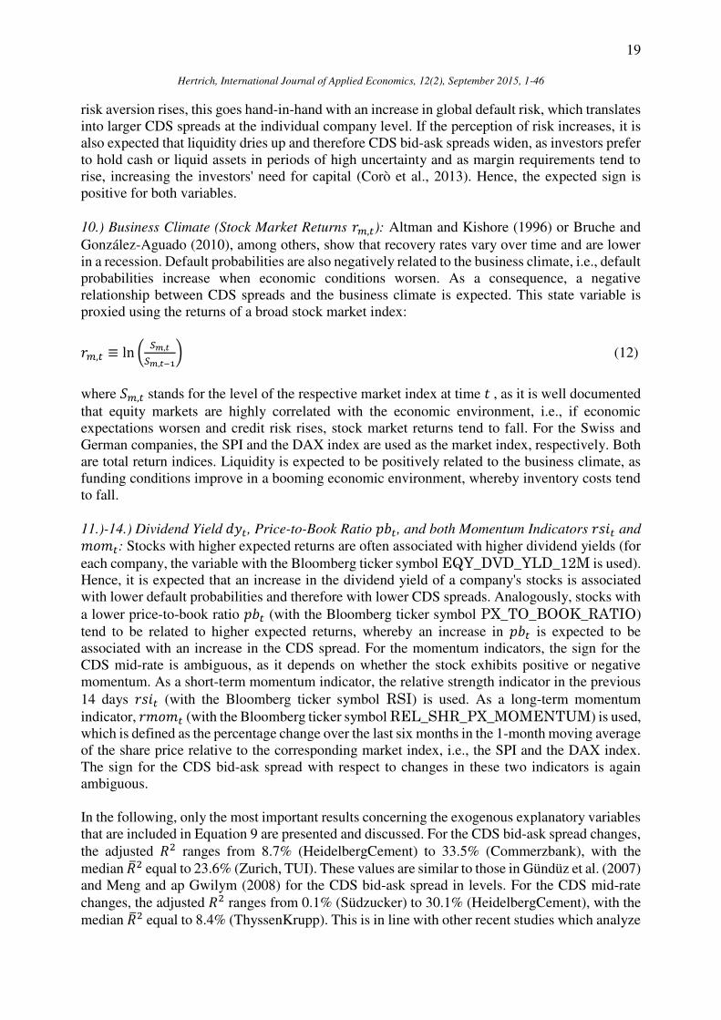
A closer look at the bid-ask spread changes (the first differences) in Figures 3 and 4 reveals that

the data exhibit volatility clustering, especially in the aforementioned periods.

In Figures 5 and 6, the credit risk proxy (the CDS mid-rate) is plotted for the Swiss and the

German companies, respectively. In general, the mid-rate is less volatile than the bid-ask spread

(compare Figures 1 or 2 with Figures 5 or 6) and larger in absolute value, as it is the mean of two

positive prices, as opposed to the absolute value of the difference between the two. In the case of

UBS (panel 4 in Figure 5), Merck and VW (panels 2 and 4 in Figure 6), the CDS mid-rate even

rises above 300 bps in some periods. In addition, there are periods where the time series seem to

be non-stationary (for example, in spring 2008 or around the end of 2008 in Figures 5 or 6, where

soaring mid-rates are observed, which also become more volatile) and periods where this is not

the case. The stationarity test results in Section 5.1 supports this conjecture.

Assuming conservatively that approximately 4% of the CDS spread compensates for liquidity

risk (Bühler and Trapp, 2009), there are periods where the liquidity risk premium was between

10-16 bps (Figures 5 and 6), but could well be as large as 33-52 bps, for example, by applying

the estimates in Lin et al. (2011).

This section concludes with the plot of the daily changes (first differences) of the mid-rate of the

corresponding four Swiss and German companies in Figures 7 and 8, respectively. As it is the

case with the changes in the bid-ask spread, the changes in the mid-rate exhibit volatility clusters.

Compared to the changes in the bid-ask spread, however, the changes in the mid-rate are more

pronounced (compare Figures 3 and 4 with Figures 7 and 8, respectively).

11 For a detailed description of this database and a comparison of this database with five alternative major sources,

please refer to the study of Mayordomo et al. (2014). 12 The computations in this paper were performed using the software package R (version 3.0.0).

11


5. Empirical Results

5.1 Univariate Time Series Properties: Order of Integration and Autocorrelation Bid-Ask Spread Stationarity: As the correct critical values of the KPSS test depend on the

deterministic component and in accordance with Figures 1, 2, 5 and 6, first it is checked whether

a time trend is present in both the bid-ask spread and the mid-rate (these figures are not included

in this paper).13 Based on these figures, an intercept is included under the null hypothesis of level

stationarity. Table B.1 in Appendix B reveals that the levels of the bid-ask spread are non-

stationary according to the KPSS test, whereas the changes are stationary (Table B.2 in Appendix

B). This finding accords with, for example, Chordia et al. (2000), Blanco et al. (2005) and Corò

et al. (2013), among others, but contrasts with Hasbrouck and Seppi (2001), Tang and Yan

(2007), Acharya and Johnson (2007) or Pires et al. (2010). The results for the other companies in

the sample (results not included) are similar to the presented results.

To date, there is no consensus as to whether the CDS bid-ask spread should be stationary or not.

In view of this, and in accordance with the test results and in order to exclude the possibility of

spurious results (see, e.g., the aforementioned study by Toda and Phillips (1993)), in the

following it is assumed that the bid-ask spread is integrated of order 1. Also the fact that both the

bid-ask spread and the mid-rate are time series that are bounded from zero supports this decision,

as in this case conventional unit root tests reject the null hypothesis of a unit root too often, even

asymptotically, and more adequate unit root tests in the spirit of Cavaliere and Xu (2014) are

required. Accordingly, the asymptotic power of conventional stationarity tests should also be

lower than when dealing with unbounded time series.

As is evident, the bid-ask spread exhibits a large number of zero changes and may better be

described by a discrete time series with more frequent zero changes (see Figures 1, 2, 3, 4 and

Table B.3 in Appendix B) than what is generally assumed in conventional time series tests, which

may bias the results. For instance, the simulation study by Annaert et al. (2004), who analyze

how commonly used normality tests detect deviations from normality, indicates that if a given

time series, which under the null hypothesis follows a geometric Brownian motion, is rounded to

the nearest cent (this corresponds to a tick size of 1 cent for equities), the Jarque-Bera test, for

instance, will be biased if the discreteness of the data is ignored.14 There are, however, only a few

studies that emphasize this potential problem; see Huberman and Halka (2001), among others.

Mid-Rate Stationarity: The KPSS test for the mid-rate in levels and for the first differences in

Tables B.1 and B.2 in Appendix B indicates that the mid-rate is integrated of order 1. In both

cases, an intercept is included under the null hypothesis. The KPSS test results accords with the

test results in the rest of the sample (test results not included). As a robustness check, other unit

root tests are applied that support this result (test results not included).

These results accord with the time series properties of the CDS spreads data in Blanco et al.

(2005), Greatrex (2009) or Norden and Weber (2009), among others. Mayordomo et al. (2014)

analyze a similar period than in the present study, namely the period after August 9, 2007 until

13 To save space, some figures and test results have been omitted in the text, but most of them are part of a separate

supplement. 14 In addition, the discreteness of the data may require alternative central limit theorems, see, e.g., Chapter 5 in Judge

et al. (1985).

12


March 29, 2010,15 and use a sample that includes one Swiss and 13 German companies which

are also contained in this study. They also conclude that the CDS mid-rates in their sample are

best described by a unit-root process, except for Commerzbank.16 Hence, in the following, this

study assumes that the mid-rate has a unit root.

Concluding this section, in the following, it is assumed that the time series in the used data sample

are all integrated of order 1. To complement the univariate time series properties, this study also

applies the unit root test developed by Zivot and Andrews (1992) that allows for a single break

in the intercept, the trend or both. The test results do support the null hypothesis of a unit root in

the original time series (the test statistics of both the cointegration test and the unit root test

allowing for a single break are part of a separate supplement). In addition, also a cointegration

analysis is performed to analyze whether the bid-ask spread and the mid-rate are cointegrated.

The test results, however, reject this hypothesis.17

Bid-Ask Spread and Mid-Rate Autocorrelation: Using the Ljung-Box test, it is further analyzed

whether the changes in the bid-ask spread (∆𝐵𝐴𝑆) and the mid-rate (∆𝑀𝐼𝐷) are serially

correlated. As the sample is sufficiently large (there are in total 723 observations), 20 lags are

used. The test results in Table B.4 in Appendix B clearly reject the null hypothesis of serially

uncorrelated time series. Therefore, when performing the causality tests in Sections 5.3 and 5.4,

more than one lag of the variables ∆𝐵𝐴𝑆 and ∆𝑀𝐼𝐷 are included.

5.2 Cross-Correlation between Credit Risk and Liquidity Risk

In this section, the Granger causality analysis in Sections 5.3 and 5.4 is motivated by analyzing

the correlation between the bid-ask spread changes and the mid-rate changes for up to 25 leads

and lags by means of the cross-correlation function (CCF):

𝜌∆𝐵𝐴𝑆,∆𝑀𝐼𝐷(𝑖) = 𝛾∆𝐵𝐴𝑆,∆𝑀𝐼𝐷(𝑖)𝜎∆𝐵𝐴𝑆∙𝜎∆𝑀𝐼𝐷 (10)

for 𝑖 = 0, ±1, ±2, … ± 25. 𝛾∆𝐵𝐴𝑆,∆𝑀𝐼𝐷(𝑖) denotes the cross-covariance function between ∆𝐵𝐴𝑆

and ∆𝑀𝐼𝐷 at lead or lag ±𝑖 and 𝜎∆𝐵𝐴𝑆 and 𝜎∆𝑀𝐼𝐷 denote the corresponding standard deviations.

The CCF measures the strength and the direction of the correlation between both time series. It

is shown that there are significant leads and lags of the bid-ask spread changes and/or the mid-

rate changes to help predict the next periods' realizations.

As seen in Section 5.1, the data are both difference-stationary and exhibit a large degree of

persistence. In addition, it is assumed that the cross-covariance 𝛾∆𝐵𝐴𝑆,∆𝑀𝐼𝐷(𝑖) between the bid-

ask spread changes and the mid-rate changes only depends on the time difference, such that the

CCFs can be calculated. At lag 0, the CCF displays the contemporaneous correlation between the

changes in the bid-ask spread and the mid-rate. At a negative lag 𝑖 < 0, the CCF measures the

correlation between the bid-ask spread changes at time 𝑡, ∆𝐵𝐴𝑆𝑡, and the mid-rate changes at a

date before time 𝑡 (∆𝑀𝐼𝐷𝑡+𝑖 [ = ∆𝑀𝐼𝐷𝑡−|𝑖|]). Analogously, at a positive lag 𝑖 > 0, the CCF

15 They do not explicitly state the exact start and end date. Given their information and the number of observations,

it is assumed that they analyze the period from September 14, 2007 to March 29, 2010. 16 For the Commerzbank mid-rate, however, the KPSS test and several unit root tests in R indicate that the data are

non-stationary. 17 Also in this case, the conventional cointegration tests suffer from size distortions (Cavaliere, 2006). However, as

the distance to the lower bound is large, the standard methods are still appropriate.

13


measures the correlation between the bid-ask spread changes at time 𝑡 (∆𝐵𝐴𝑆𝑡) and the mid-rate

changes at a date after time 𝑡 (∆𝑀𝐼𝐷𝑡+𝑖).

In Figures 9 and 10, the CCFs for ∆𝐵𝐴𝑆 and ∆𝑀𝐼𝐷 for the four Swiss and four German

companies in the sample are plotted. In each figure, the corresponding 95% confidence interval

is included. For the Swiss companies (Figure 9), there are significant correlation coefficients

between both measures at lag 1 or 2 with alternating and varying signs, except for ABB (panel 1

in Figure 9). In the case of ABB, only a contemporaneous correlation between ∆𝐵𝐴𝑆 and ∆𝑀𝐼𝐷

can be detected. For Nestlé (panel 2 in Figure 9), the second lag coefficient (𝑖 = 2) is negative

and significantly different from zero, indicating that the changes in the bid-ask spread two periods

ago help to predict the changes in the mid-rate in period zero. For Roche (panel 3 in Figure 9),

the changes in the mid-rate in the previous periods (𝑖 < 0) help to predict the change in the bid-

ask spread in the following period, although with alternating and varying signs. For UBS,

predictability is detected for both variables (panel 4 in Figure 9), but again with varying and

alternating signs.

The results for the German companies (Figure 10) reveal a different picture. Ignoring significant

coefficients at higher leads and lags, these data only exhibit a contemporaneous correlation

among both measures, except for VW. For VW (panel 4 in Figure 10), the first lag coefficient

(𝑖 = −1) is positive and significant, indicating that the changes in the mid-rate one period ago

help to predict the changes in the bid-ask spread in period zero. For the other three German

companies, the correlation at lag 0 is shown to be both significantly different from zero and

positive. Only the magnitude of the contemporaneous cross-correlation differs across companies.

For Deutsche Bank, Merck, Siemens and VW, the cross-correlation coefficient approximately

equals 0.22, 0.4, 0.3 and 0.16, respectively.

Concluding this section, notice that the results in this section suggest that analyzing the lead-lag

relationship between the changes in the bid-ask spread and the changes in the mid-rate in order

to identify whether liquidity risk changes are endogenous with respect to credit risk changes or

not, and vice versa, is a worthwhile exercise.

5.3 Granger Causality Test: Testing Credit Risk and Liquidity Risk for Exogeneity

In this section, it is finally tested whether liquidity changes are weakly exogenous in the time

series sense (Hamilton, 1994) with respect to credit risk changes. This is done following the

methodology described in Section 3. Section 5.1 showed that in the present data sample both the

bid-ask spread and the mid-rate are integrated of order 1 and that they are both not cointegrated.

As a consequence, first differences are used to perform the Granger causality test. The causality

test results for the null hypothesis that changes in the bid-ask spread do not Granger-cause

changes in the mid-rate (∆𝐵𝐴𝑆 𝐺𝑟𝐶⇏ ∆𝑀𝐼𝐷) and vice versa (∆𝑀𝐼𝐷 𝐺𝑟𝐶⇏ ∆𝐵𝐴𝑆) are given in Tables

1 and 2 for the Swiss and German companies, respectively.

The Granger causality test shows that the changes in the CDS mid-rate (∆𝑀𝐼𝐷) Granger-cause

the changes in the CDS bid-ask spread (∆𝐵𝐴𝑆) for approximately 46% of the Swiss companies

(Table 1) and 35% of the German companies (Table 2) at the 5% significance level (or 39% in

total). The number increases to approximately 54% and 52%, respectively, if a significance level

of 10% (or 52% in total) is chosen. In contrast, the changes in the bid-ask spread are significant

at the 5% significance level only for Kabel Deutschland (Table 2) and at the 10% significance

level for Swiss Re (Table 1), Bayer and Munich Re (Table 2). For Swiss Re, Kabel Deutschland

and Munich Re, even a feedback relationship is detected. It is interesting that in this sample a

14


feedback relationship for two of the three most important reinsurance companies in the world is

found.18 This may deserve further investigation, as Jarrow (2011) argues that counterparty risk

in the CDS market may be mitigated by introducing the requirement of 100% of the notional

amount as collateral, which is the standard practice in reinsurance contracts, meaning that this

industry exhibits special features that may in part explain this phenomenon. These results also

extend previous findings in Breitenfellner and Wagner (2012), among others, who find that

liquidity proxies are only relevant for CDS spread changes for financial companies. First, a

reverse Granger causality is detected in this sample, second, it is found that also for financial

companies the used liquidity proxy does not Granger-cause CDS spread changes (see Tables 1

and 2 below for the relevant companies, and Tables A.1 and A.2 in Appendix A for the assigned

industry classification of these companies).

It is interesting to observe that UBS, the bank that had to be rescued by the Swiss National Bank

in October 2008, is the sole bank in this sample, where credit risk changes are not (weakly)

endogenous with respect to liquidity risk changes. However, also Commerzbank has been bailed

out by the German government in January 2009, where the reported results imply that credit risk

changes are (weakly) endogenous with respect to liquidity risk changes.

In sum, these results indicate that credit risk shocks are followed by a subsequent liquidity

shortage in the CDS market. However, liquidity shocks in general do not Granger-cause credit

risk changes. Hence, in this sample liquidity or liquidity risk seems to be rather (weakly)

exogenous than endogenous for credit risk changes. Consequently, these findings support

previous ad hoc assumptions that liquidity is (weakly) exogenous with respect to credit risk

changes, but also show that in credit markets, credit risk might be endogenous with respect to

liquidity risk, in the spirit of, e.g., the liquidity spiral posited by Brunnermaier (2009).

For the companies that experienced no change in credit rating,19 the results show that credit risk

is endogenous with respect to liquidity risk in 58% (or 67% at the 10% significance level) of the

cases, compared to 31% (or 47% at the 10% significance level) in the case of the companies that

suffered a credit rating change. This is consistent with the findings in Beber et al. (2009), who

disentangle the effect of a flight-to-quality from the effect of a flight-to-liquidity for Euro-area

government bonds in periods of heightened uncertainty. They document that in these periods

investors' demand for liquid assets dominates the demand for credit quality. Although their

sample analyzes a different environment than in the present study, the empirical results in this

analysis indicate that a credit shock widens the bid-ask spread substantially in the subsequent

days, consistent with the market microstructure literature view that in times of heightened

uncertainty bid-ask spreads rise. This effect is more pronounced among the companies with a

stable credit rating, whereas there's no difference between high- and low-rated companies,

meaning that the credit rating per se is of secondary relevance in determining changes in liquidity,

which may deserve additional research.

To provide further information about the relationship between credit risk and liquidity risk, the

orthogonalized impulse response functions (IRFs) are displayed in Figures 11-18 for 𝑖 =0, 1, … , 10 steps ahead. Focusing on the corresponding panels 2 and 3 in each figure, the graphical

results in panel 2 in all the figures show that positive innovations in credit risk on the previous

day (∆𝑀𝐼𝐷 > 0) are followed by a deterioration of liquidity (∆𝐵𝐴𝑆 > 0) on the following day.

18 According to the gross premiums written in 2011, Munich Re is the largest reinsurance company in the world,

followed by Swiss Re and Hannover Rück. 19

These are Credit Suisse, Swisscom, Allianz, Bayer, E.ON, EnBW, Fresenius, Hannover Rück, Lanxess, Munich

Re, Siemens and Südzucker.

15


As a consequence, the coefficient at lag 1 is positive and in most cases significantly different

from zero, but numerically small. As expected, the credit risk innovations do not have a

sustainable effect on the equation system, as in most cases the effect fades away after the second

or third day. The response of credit risk to a liquidity risk innovation, however, is different. In

most cases, the response is not significantly different from zero (panel 3 in all the figures).

Resuming this section, the presented results imply that credit risk and illiquidity are positively

correlated. This result is in line with the findings of Cherubini and DellaLunga (2001), Boss and

Scheicher (2002), and Ericsson and Renault (2006), among others (see Section 2.1.3 for more

details). To be more specific, it seems that in the short run credit risk changes are more likely to

induce CDS market liquidity to dry-up than vice versa. This is interesting, as this observation

indicates that a liquidity shortage may be preceded by credit risk shocks, in the spirit of the

liquidity spiral in Brunnermaier (2009). Hence, a deterioration in credit risk, as was observed

during the beginning of the current financial crisis, may trigger a liquidity crisis in the CDS

market. This linkage may be one of the amplifying mechanisms that aggravated and propagated

the initial credit shocks in the subprime market. Brunnermaier (2009), for instance, describes an

economic balance sheet mechanism that shows how unexpected and initially small losses

(implying higher credit risk) can initiate a loss spiral, as highly levered companies may be forced

to sell assets to hold constant, e.g., a target leverage ratio, which may cause margins to rise, as

asymmetric-information frictions emerge. Hence, according to the microstructure literature, bid-

ask spreads rise. This loss spiral is expected to be more pronounced in relatively illiquid markets

and in periods of heightened uncertainty. This spiral then may cause the CDS market to become

illiquid. The breakdown of the CDS market may also have real effects on the economy, as CDS

contracts may enhance financial market efficiency by offering insurance against the default of

fixed-income instruments. Jaccard (2013), among others, develops a macroeconomic model that

shows how credit shocks can lead to a liquidity shortage with real effects on the macroeconomy.

Alternatively, the information amplification mechanism in Caballero and Krishnamurthy (2008)

and Krishnamurthy (2010), among others, may well describe the observed increase in the CDS

bid-ask spreads during the recent financial crisis, as it is well documented that in this period

investors started to put into question the standard CDS pricing models, after investors had

suffered unexpectedly large losses on CDS contracts and therefore closed investment positions

in the CDS market and sought more liquid assets, with the consequence that CDS bid-ask spreads

widened, consistent with the microstructure literature view that bid-ask spreads widen when the

risk of adverse selection increases. The banking model developed by Bolton et al. (2011), where

asymmetric information about asset quality (a real shock in the form of a lower quality of the

risky assets) triggers early asset sales, thereby deteriorating liquidity, also accords with the

findings of this paper.

For the other companies in the sample, where no significant lead-lag relationship between credit

risk shocks and liquidity is detected, alternative explanations, such as the model in Easley and

O'Hara (2010), where illiquidity arises from uncertainty (i.e., investors having incomplete

preferences over portfolios) or the model in He and Xiong (2012), where companies that have to

roll over maturing debt face rising credit spreads, in a market environment where liquidity in the

bond market is deteriorating, may describe the observed increase in both the CDS bid-ask spreads

and the CDS spreads during the recent financial crisis.

To sum up, the findings of this paper imply that credit risk might be (weakly) endogenous with

respect to liquidity risk, which has important consequences for the asset pricing and the risk

management literature. For example, a liquidity-enhanced CAPM or a value-at-risk model that

16


includes illiquidity as an additional variable should treat liquidity as endogenous and control for

the interaction between credit and liquidity risk, which contradicts the standard practice until

now. Also for policy-makers, the indication that a negative credit shock may cause a liquidity

shortage in the CDS market should be taken into account when setting capital requirements for

financial institutions. In addition, when pricing derivatives that are related to assets with credit

risk the results in this study imply that liquidity risk may be an important factor to include and to

control for its interaction with credit risk.

5.4 Model Extension

If an important variable that is correlated with one of the dependent variables and one of the

included regressors is omitted, a spurious Granger causality among the endogenous variables

may be found, as the effect of omitted variables is contained in the innovations (see, e.g.,

Lütkepohl (2007)). Therefore, in the following, the robustness of the reported causality test

results are analyzed, with a special focus on the changes in the CDS mid-rate. For the changes in

the CDS bid-ask spread, most of the commonly used explanatory variables are not available from

Bloomberg and Datastream. To gain additional insights, however, this study checks how the

included financial and macroeconomic explanatory variables that determine the changes in the

CDS mid-rate impact the CDS bid-ask spread. As previously commented, there are only two

studies that analyze the determinants of the CDS bid-ask spreads. Hence, the results of this study

add to the strand of literature that analyzes liquidity in CDS markets.

To control for potential omitted variables bias, the VAR(𝑝) model is extended by introducing

variables suggested by finance theory and variables that have been proven to be important in

explaining the variation in CDS spreads in empirical studies. The data is obtained from

Bloomberg and covers the same period as before. The extended VAR(𝑝) model (denominated as

VARX(𝑝) model) includes some of the key variables that in the Merton-type structural models

for default determine credit spreads. These are the risk-free interest rate, the degree of leverage

and the volatility of the firm's assets' value. In more general models, additional state variables are

included to capture the stochastic volatility of the firm's assets' value or the randomness of the

risk-free interest rate.20 Therefore, the VARX(𝑝) model includes commonly used state variables,

such as the slope of the yield curve, the TED spread, the default yield spread, an index of stock

market option-implied volatility, and the returns of a broad stock market index as a proxy for the

business climate. Moreover, the VARX(𝑝) model also includes variables that are commonly

associated with expected returns; i.e., the dividend yield, the price-to-book ratio and two

momentum indicators (one short-term and one long-term indicator) of the companies in the

sample, since Collin-Dufresne et al. (2001) and Campbell and Taksler (2003), among others,

show that credit spreads are partly determined by equity-related variables. Since both the changes

in the CDS bid-ask spread and the CDS mid-rate are analyzed, the first differences of these

variables are taken in order to be consistent with this strand of literature. In the following, the

exogenous variables are described and it is explained what their expected impact on the changes

in the CDS bid-ask rate and in the CDS mid-rate is. Table C.1 in Appendix C summarizes the

expected signs for all the included exogenous explanatory variables.

1.) Risk-Free Interest Rate 𝑟𝑡𝑓: A higher risk-free interest rate 𝑟𝑡𝑓

raises the discount rate and

therefore reduces the value of bonds. Hence, for a given firm value, if the interest rate rises, the

distance to default increases. Given that in the Merton model the firm value process grows with

20 In the original Merton model, no state variables are necessary, as the risk-free rate is assumed to be constant over

time.

17


the risk-neutral interest rate, the expected growth rate of the firm's value will also adjust

accordingly. Hence, for a given notional amount, the risk-neutral default probability will fall

(Longstaff and Schwartz, 1995). Therefore, CDS spreads should in general fall with a higher risk-

free interest rate 𝑟𝑡𝑓. This conjecture has been empirically proven in Skinner and Townend (2002)

and Ericsson and Renault (2006), among others. The (short-term) risk-free interest rate is proxied

by the 3-month EUR LIBOR interest rate,21 following the practice of derivative traders, among

others. For the CDS bid-ask spread, this paper conjectures that higher risk-free interest rates, as

a proxy for the inventory costs associated with holding overnight positions, cause bid-ask spreads

to widen, in line with Bessembinder (1994), among others.

2.) Leverage and Firm Value (Stock Returns 𝑟𝑡): In the structural framework, default is triggered

whenever the leverage ratio equals or falls below one. Consequently, the larger the firm value is

for a given debt level, the larger the distance to default, which is an inverse representation of the

default probability. Hence, CDS spreads should rise, whenever the leverage ratio increases. As

in the structural framework total firm value equals total debt plus equity, this implies that the

return on equity should be negatively related to CDS spreads.22 As accounting data are not

available at a daily frequency, changes in the firm's financial health are proxied by the company's

continuously compounded equity returns, following, e.g., Blanco et al. (2005):

𝑟𝑡 ≡ ln ( 𝑆𝑡𝑆𝑡−1) (11)

where 𝑆𝑡 stands for the stock price of the reference entity at time 𝑡. Some studies, however,

linearly interpolate low-frequency data to obtain higher frequency data, see Collin-Dufresne

(2001) or Greatrex (2009), among others. Given that this paper works with daily data, this

approach makes little sense. The expected negative relationship between equity returns and credit

spreads is supported by the empirical findings in Ericsson and Renault (2006), among others.

With reference to the CDS bid-ask spread, a higher leverage ratio (or lower stock returns) is

expected to cause CDS liquidity to worsen (see Section 2.1.3), consistent with the empirical

evidence from U.S. bond markets provided by Hong and Warga (2000). Indeed, Brunnermaier

and Pedersen (2009) report that positive stock returns increase the availability of capital that

market makers use to fund their trading positions, thereby lowering the bid-ask spread.

3.)-5.) Asset Volatility (Stock Volatility 𝜎𝑡): In the structural framework, the volatility 𝜎 of the

firm's assets equals the volatility of the sum of debt and equity. This variable is proxied by the

historical short-term and long-term equity return volatility 𝜎𝑡30 and 𝜎𝑡360, i.e., the volatility of

each company's stock returns for the most recent 30 and 360 trading days.23 Cremers et al. (2008)

show empirically that the individual stock option-implied volatility is an important determinant

of credit spreads. Therefore also the implied volatility 𝜎𝑡𝑖𝑚𝑝 of each company's stock options with

a time to maturity of three months is included, following Pires et al. (2010) and Hibbert et al.

(2011), among others. In the structural framework, since the value of debt equals risk-free debt

plus a short position in a credit put option with an exercise price equal to the face value of debt,

credit spreads should rise with volatility, because the short put price decreases when volatility

21 It can be argued that for 5-year CDS contracts, the risk-free interest rate 𝑟𝑡𝑓

should instead be a long-term interest

rate, e.g., the expected return on a default-free 5-year zero coupon bond. The present study, however, follows the

standard practice in this strand of literature. 22

As changes in the debt value should be transmitted one to one to the equity value. In addition, lower stock returns

suggest that a firm's future business is expected to worsen, whereby default risk would rise. 23

This implies that it is assumed that the volatility of debt approximately equals minus two times the covariance

between debt and equity.

18


rises. This is also intuitive, as the larger the volatility becomes, the more likely it is that the firm's

asset value will fall below its debt value, meaning that the probability of default is positively

related to volatility. For the CDS bid-ask spread, a positive relationship is expected as well, since

Stoll (2000), among others, finds a positive relationship between bid-ask spreads and the level of

stock market volatility. In the following, the state variables that are included in the VARX(𝑝)

model are motivated and described.

6.) Slope of the Yield Curve 𝑠𝑙𝑡: It is commonly accepted that the level and the slope of the yield

curve explain a large portion of the bond return variability. This conjecture has been analyzed

and empirically proven for U.S. bonds by Litterman and Scheinman (1991). Although the slope

does not enter the equation of the firm value process in the Merton model, the risk-free interest

may well depend on the characteristics of the yield curve. If an increase in the slope causes the

expected future risk-free rate to rise, CDS spreads may decrease (see the previous reasoning for

the risk-free interest rate). Hence, a negative relationship between the slope of the yield curve 𝑠𝑙𝑡

and the CDS mid-rate may be expected. This conjecture is supported by the empirical findings in

Ericsson and Renault (2006), among others. In addition, a steeper yield curve is commonly

interpreted as the expectation of a booming economy. As a consequence, the recovery rate is

expected to rise and the default probability to fall. Hence, CDS spreads should fall. Fama and

French (1989), among others, find that default spreads widen when overall economic conditions

worsen. For the CDS bid-ask spread, this paper conjectures that a better economic outlook is

associated with lower funding costs, in the spirit of Brunnermaier and Pedersen (2009), among

others. Hence, the CDS bid-ask spread should be negatively related to the slope of the yield curve.

The slope of the yield curve 𝑠𝑙𝑡 is proxied by the yield difference between the 10-year constant

maturity EMU government bond yield and the 1-year constant maturity EMU government bond

yield.

7.) TED Spread 𝑡𝑒𝑑𝑡: Due to its relevance in integrated global financial markets, the U.S. TED

spread is used, i.e., the 3-month USD LIBOR interest rate minus the 3-month U.S. Treasury Bill

rate, as a proxy for funding illiquidity (Brunnermaier, 2009). As already mentioned, this paper

expects that an increase in funding illiquidity is accompanied by an increase in both the CDS

mid-rate and the CDS bid-ask spread. Hence, a positive sign is expected for the impact of this

variable on both aforementioned CDS variables.

8.) Default Yield Spread 𝑑𝑠𝑝𝑟𝑒𝑎𝑑𝑡: This paper also controls for the portion of credit risk that is

related to aggregate (market) default risk. This risk factor is proxied by the spread between

Moody's Baa Corporate Bond Yield Index and Moody's Aaa Corporate Bond Yield Index. In line

with the reasoning in Section 2.1.3, a positive relationship between this variable and the level of

CDS spreads is expected. Hence, changes in both of these variables should also be positively

correlated. As mentioned in the theoretical part of this chapter (Section 2.1.3), the expected sign

on the liquidity risk proxy is ambiguous. However, due to the argumentation in Section 2.1.3,

this paper conjectures a positive sign, i.e., that an increase in systematic credit risk is related to a

decrease in liquidity.

9.) Stock Market Option-Implied Volatility 𝑣𝑑𝑎𝑥𝑡: In periods of financial turmoil, risk aversion

rises and a "flight-to-quality" is expected, i.e., an increase in the demand for more liquid assets,

which has been documented by Longstaff (2004) for U.S. Treasury bonds, among others. Option-

implied volatility indices are commonly used as risk aversion measures. For the option-implied

volatility of European stock markets, the DAX Volatility Index (VDAX index) is used, which

measures the implied volatility of DAX index options. It is quoted in percentage points per annum

and represents the expected movements in the stock market over the next 30-day period. If global

19


risk aversion rises, this goes hand-in-hand with an increase in global default risk, which translates

into larger CDS spreads at the individual company level. If the perception of risk increases, it is

also expected that liquidity dries up and therefore CDS bid-ask spreads widen, as investors prefer

to hold cash or liquid assets in periods of high uncertainty and as margin requirements tend to

rise, increasing the investors' need for capital (Corò et al., 2013). Hence, the expected sign is

positive for both variables.

10.) Business Climate (Stock Market Returns 𝑟𝑚,𝑡): Altman and Kishore (1996) or Bruche and

González-Aguado (2010), among others, show that recovery rates vary over time and are lower

in a recession. Default probabilities are also negatively related to the business climate, i.e., default

probabilities increase when economic conditions worsen. As a consequence, a negative

relationship between CDS spreads and the business climate is expected. This state variable is

proxied using the returns of a broad stock market index:

𝑟𝑚,𝑡 ≡ ln ( 𝑆𝑚,𝑡𝑆𝑚,𝑡−1) (12)

where 𝑆𝑚,𝑡 stands for the level of the respective market index at time 𝑡 , as it is well documented

that equity markets are highly correlated with the economic environment, i.e., if economic

expectations worsen and credit risk rises, stock market returns tend to fall. For the Swiss and

German companies, the SPI and the DAX index are used as the market index, respectively. Both

are total return indices. Liquidity is expected to be positively related to the business climate, as

funding conditions improve in a booming economic environment, whereby inventory costs tend

to fall.

11.)-14.) Dividend Yield 𝑑𝑦𝑡, Price-to-Book Ratio 𝑝𝑏𝑡, and both Momentum Indicators 𝑟𝑠𝑖𝑡 and 𝑚𝑜𝑚𝑡: Stocks with higher expected returns are often associated with higher dividend yields (for

each company, the variable with the Bloomberg ticker symbol EQY_DVD_YLD_12M is used).

Hence, it is expected that an increase in the dividend yield of a company's stocks is associated

with lower default probabilities and therefore with lower CDS spreads. Analogously, stocks with

a lower price-to-book ratio 𝑝𝑏𝑡 (with the Bloomberg ticker symbol PX_TO_BOOK_RATIO)

tend to be related to higher expected returns, whereby an increase in 𝑝𝑏𝑡 is expected to be

associated with an increase in the CDS spread. For the momentum indicators, the sign for the

CDS mid-rate is ambiguous, as it depends on whether the stock exhibits positive or negative

momentum. As a short-term momentum indicator, the relative strength indicator in the previous

14 days 𝑟𝑠𝑖𝑡 (with the Bloomberg ticker symbol RSI) is used. As a long-term momentum

indicator, 𝑟𝑚𝑜𝑚𝑡 (with the Bloomberg ticker symbol REL_SHR_PX_MOMENTUM) is used,

which is defined as the percentage change over the last six months in the 1-month moving average

of the share price relative to the corresponding market index, i.e., the SPI and the DAX index.

The sign for the CDS bid-ask spread with respect to changes in these two indicators is again

ambiguous.

In the following, only the most important results concerning the exogenous explanatory variables

that are included in Equation 9 are presented and discussed. For the CDS bid-ask spread changes,

the adjusted 𝑅2 ranges from 8.7% (HeidelbergCement) to 33.5% (Commerzbank), with the

median �̅�2 equal to 23.6% (Zurich, TUI). These values are similar to those in Gündüz et al. (2007)

and Meng and ap Gwilym (2008) for the CDS bid-ask spread in levels. For the CDS mid-rate

changes, the adjusted 𝑅2 ranges from 0.1% (Südzucker) to 30.1% (HeidelbergCement), with the

median �̅�2 equal to 8.4% (ThyssenKrupp). This is in line with other recent studies which analyze

20


the determinants of CDS spread changes, see Ericsson et al. (2009) and Corò et al. (2013), among

others.

When including the previously presented exogenous explanatory variables, the causal structure

remains qualitatively unchanged (compare Tables 1 and 2 with Tables C.2 and C.3 in Appendix

C). A plot of both the orthogonalized and the cumulative orthogonalized IRFs (this figures are

available from the author upon request) reveals that the dynamic interaction between credit risk

and liquidity risk and the VARX(𝑝) coefficients remain essentially unchanged. This observation

supports the main conclusions of this paper. In both the VAR model as well as in the VARX

model the results indicate that new information is quickly reflected in the CDS bid-ask spreads

and in the CDS mid-rates, as in most cases, only the respective first autoregressive lags are

significant.

Apart from the corresponding lags of the CDS bid-ask spread changes and the CDS mid-rate

changes, the most relevant explanatory variables are the changes in the stock returns (∆𝑟𝑡), the

changes in the long-term equity return volatility (∆𝜎𝑡360), the changes in the slope of the yield

curve (∆𝑠𝑙𝑡), the changes in the TED spread (∆𝑡𝑒𝑑𝑡), the changes in the default yield spread

(∆𝑑𝑠𝑝𝑟𝑒𝑎𝑑𝑡) and the changes in the market stock returns (∆𝑟𝑚,𝑡). In general, the relevance of the

other explanatory variables is negligible. Therefore, in the following, only the results for the most

relevant exogenous explanatory variables are presented and also only for the relevant equation in

the VARX model.

In general, the coefficient for the changes in the stock returns (∆𝑟𝑡) of the reference entity is in

line with the expected sign. Higher stock returns are accompanied by a decrease in both the CDS

bid-ask spreads and the CDS mid-rates. This observation accords with the aforementioned

hypothesis that a higher company value decreases the default probability and increases the

availability of capital that market makers can use to fund their trading positions.

Changes in the long-term volatility (∆𝜎𝑡360) are, in general, a relevant explanatory variable for

the changes in the CDS mid-rate only. The coefficients are in line with the expected sign, i.e.,

higher asset volatility (proxied by the stock volatility) increases the probability of default and

therefore CDS mid-rates tend to increase.

For the slope of the yield curve, the results indicate that a steeper yield curve (∆𝑠𝑙𝑡 > 0) precedes

a decrease in the CDS mid-rate. This finding is in line with the corresponding hypothesis in Table

C.1 and the findings in Abid and Naifar (2006), among others, who analyze CDSs from different

countries. It also accords with Ericsson et al. (2009) and in part with the results in Breitenfellner

and Wagner (2012), but is contrary to the findings of, for example, Collin-Dufresne et al. (2001)

and Oliveira et al. (2012) for Eurozone government credit spreads or Di Cesare and Guazzarotti

(2010), who analyze CDS contracts for U.S. non-financial firms and find that an increase in the

slope of the yield curve is followed by an increase in the CDS mid-rate.

Interestingly, the coefficients for the changes in the TED spread (∆𝑡𝑒𝑑𝑡 > 0), an important proxy

variable for the degree of funding illiquidity, contradicts the conjectured sign, as an increase in

the TED spread is in general accompanied by a decrease in the CDS mid-rate.

The importance of the systematic credit risk component, proxied by the changes in the default

yield spread (∆𝑑𝑠𝑝𝑟𝑒𝑎𝑑𝑡), accords with the findings in Di Cesare and Guazzarotti (2010), among

others, who document that subsequent to the financial crisis the relevance of a common credit

risk factor has increased. In the sample of this study, this variable is significant for both the CDS

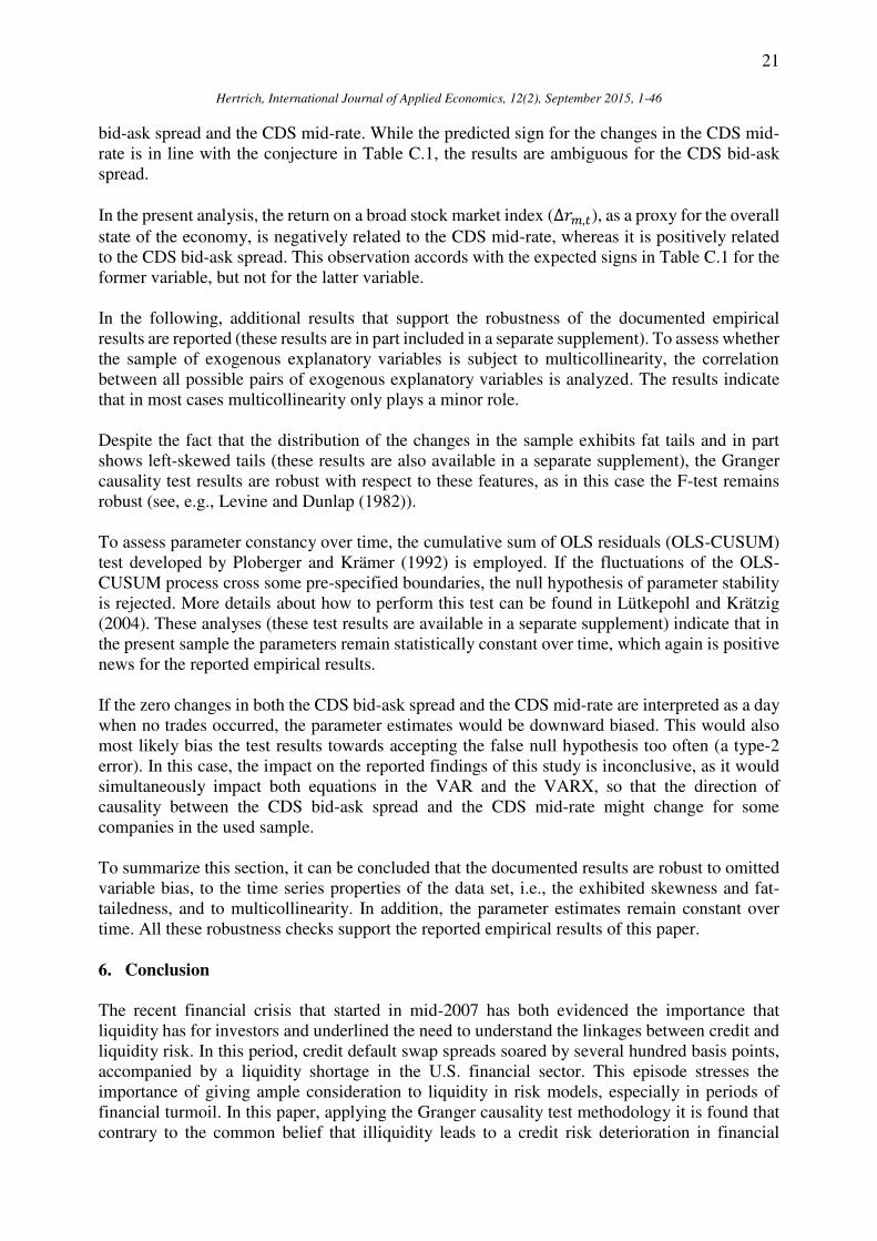
21


bid-ask spread and the CDS mid-rate. While the predicted sign for the changes in the CDS mid-

rate is in line with the conjecture in Table C.1, the results are ambiguous for the CDS bid-ask

spread.

In the present analysis, the return on a broad stock market index (∆𝑟𝑚,𝑡), as a proxy for the overall

state of the economy, is negatively related to the CDS mid-rate, whereas it is positively related

to the CDS bid-ask spread. This observation accords with the expected signs in Table C.1 for the

former variable, but not for the latter variable.

In the following, additional results that support the robustness of the documented empirical

results are reported (these results are in part included in a separate supplement). To assess whether

the sample of exogenous explanatory variables is subject to multicollinearity, the correlation

between all possible pairs of exogenous explanatory variables is analyzed. The results indicate

that in most cases multicollinearity only plays a minor role.

Despite the fact that the distribution of the changes in the sample exhibits fat tails and in part

shows left-skewed tails (these results are also available in a separate supplement), the Granger

causality test results are robust with respect to these features, as in this case the F-test remains

robust (see, e.g., Levine and Dunlap (1982)).

To assess parameter constancy over time, the cumulative sum of OLS residuals (OLS-CUSUM)

test developed by Ploberger and Krämer (1992) is employed. If the fluctuations of the OLS-

CUSUM process cross some pre-specified boundaries, the null hypothesis of parameter stability

is rejected. More details about how to perform this test can be found in Lütkepohl and Krätzig

(2004). These analyses (these test results are available in a separate supplement) indicate that in

the present sample the parameters remain statistically constant over time, which again is positive

news for the reported empirical results.

If the zero changes in both the CDS bid-ask spread and the CDS mid-rate are interpreted as a day

when no trades occurred, the parameter estimates would be downward biased. This would also

most likely bias the test results towards accepting the false null hypothesis too often (a type-2

error). In this case, the impact on the reported findings of this study is inconclusive, as it would

simultaneously impact both equations in the VAR and the VARX, so that the direction of

causality between the CDS bid-ask spread and the CDS mid-rate might change for some

companies in the used sample.

To summarize this section, it can be concluded that the documented results are robust to omitted

variable bias, to the time series properties of the data set, i.e., the exhibited skewness and fat-

tailedness, and to multicollinearity. In addition, the parameter estimates remain constant over

time. All these robustness checks support the reported empirical results of this paper.

6. Conclusion

The recent financial crisis that started in mid-2007 has both evidenced the importance that

liquidity has for investors and underlined the need to understand the linkages between credit and

liquidity risk. In this period, credit default swap spreads soared by several hundred basis points,

accompanied by a liquidity shortage in the U.S. financial sector. This episode stresses the

importance of giving ample consideration to liquidity in risk models, especially in periods of

financial turmoil. In this paper, applying the Granger causality test methodology it is found that

contrary to the common belief that illiquidity leads to a credit risk deterioration in financial

22


markets, for 39% of the German and Swiss companies in the used data sample, credit risk is

weakly endogenous for liquidity risk. The results show that in the short run credit risk changes

are more likely to induce CDS market liquidity to dry-up than vice versa. This finding implies

that a deterioration in credit risk, as was observed during the beginning of the current financial

crisis, may trigger a liquidity crisis in the CDS market, in the spirit of the liquidity spiral in

Brunnermaier (2009) or the information amplification mechanism in Caballero and

Krishnamurthy (2008) and Krishnamurthy (2010). These linkages may be one of the amplifying

mechanisms that aggravated and propagated the initial credit shocks in the subprime market, with

real effects on the macroeconomy. Alternatively, some companies in the used sample, where no

significant lead-lag relationship between credit risk changes and liquidity changes is detected,

the observed increase in both the CDS bid-ask spreads and the CDS spreads during the recent

financial crisis might be the result of investors that have incomplete preferences over portfolios

(Easley and O'Hara, 2010), or due to companies that have to roll over maturing debt and face

rising credit spreads when liquidity in the market has previously deteriorated (He and Xiong,

2012).

The findings of this paper imply that, for instance, a liquidity-enhanced CAPM or a value-at-risk

model that includes liquidity should treat liquidity as endogenous and control for the interaction

between credit and liquidity risk, contrary to the standard practice until now. In addition, for

policy-makers, the indication that a negative credit shock may cause a liquidity shortage in the

CDS market should be taken into account when setting capital requirements for financial

institutions. A better understanding of the market for credit risk is also crucial for policy-makers

when it comes to designing new macro-prudential policies. The empirical evidence in this paper

has the policy implication that policy-makers should cushion credit shocks during periods of

heightened uncertainty to prevent a liquidity shortage in, e.g., credit markets. In view of the

importance of CDS spreads as a strategic financial variable in the investment decision process,

the capacity to control CDS spreads could therefore be used to prevent rapid surges in CDS

market illiquidity and their consequent negative impact on financial markets in the future.

As the current crisis has shown that CDS contracts are also prone to the default of the CDS seller,

which accords with the observation of Hibbert et al. (2009) that counterparty risk becomes

especially relevant in periods of financial distress, in future research, the impact of counterparty

credit risk on the CDS spread should be assessed and the former should be disentangled from the

latter, applying the CDS valuation model proposed by Hull and White (2001), which explicitly

takes into account this additional risk factor.

Furthermore, by applying the valuation approach in Walker (2012), the analysis in this paper

could be extended to illiquid CDS contracts, whereby we could gain additional insights about the

dynamic relationship between credit risk and liquidity. In this respect, using intraday CDS data

may also extend our knowledge about how liquidity impacts credit markets and how credit

markets work in general.

The fact that discreteness is more pronounced in the case of CDS data than it is in the case of, for

example, equities necessitates the use of other testing procedures, as some studies demonstrate

that the standard testing procedures in time series analysis are biased when plugging in discrete

data (Annaert et al., 2004). Therefore, applying alternative causality tests for discrete time series

(e.g., using the Granger causality test for high-frequency data developed by de Jong and Nijman

(1997)) may be a natural extension of the present paper.

23


References

Abid, F. and N. Naifar. 2006. "The Determinants of Credit Default Swap Rates: An Explanatory

Study." International Journal of Theoretical and Applied Finance, 9 (1), 23-42.

Acharya, V. V. and T. C. Johnson. 2007. "Insider Trading in Credit Derivatives." Journal of

Financial Economics, 84 (1), 110-141.

Acharya, V. V. and L. H. Pedersen. 2005. "Asset Pricing with Liquidity Risk." Journal of


Altman, E. I. and V. M. Kishore. 1996. "Almost Everything You Wanted to Know about

Recoveries on Defaulted Bonds." Financial Analysts Journal, 52 (6), 57-64.

Amihud, Y. and H. Mendelson. 1986. "Asset Pricing and the Bid-Ask Spread." Journal of


Amihud, Y. and H. Mendelson. 1991. "Liquidity, Maturity, and the Yields on U.S. Treasury

Securities." Journal of Finance, 46 (4), 1411-1425.

Amihud, Y., H. Mendelson and L. H. Pedersen. 2005. "Liquidity and Asset Prices."

Foundations and Trends in Finance, 1 (4), 269-364.

Ang, A. 2014. "Illiquid Asset Investing." In: Asset Management. Oxford: Oxford University

Press, pp. 410-441.

Ang, A., W. N. Goetzmann and S. M. Schaefer. 2010. "The Efficient Market Theory and

Evidence: Implications for Active Investment Management." Foundations and Trends in

Finance, 5 (3), 157-242.

Annaert, J., M. D. Ceuster, P. van Roy and C. Vespro. 2013. "What Determines Euro Area

Bank CDS Spreads?" Journal of International Money and Finance, 32 (C), 444-461.

Annaert, J., A. G. Claes and M. De Ceuster. 2004. "Does the Compass Rose Pattern Matter for

Testing Normality?" In: van Straelen, R., Kesenne, S., Reyns, C. (Eds.), Kwantitatief

Bekeken. Antwerp: Garant Uitgevers, pp. 207-218.

Bangia, A., F. Diebold, T. Schuermann and J. Stroughair. 2002. "Modeling Liquidity Risk,

with Implications for Traditional Market Risk Measurement and Management." In: Figlewski, S.

and R. Levich (Eds.), Risk Management: The State of the Art. Amsterdam: Kluwer Academic

Publishers, pp. 1-13.

Beber, A., M. W. Brandt and K. A., Kavajecz. 2009. "Flight-to-Quality or Flight-to-Liquidity?

Evidence from the Euro-Area Bond Market." Review of Financial Studies, 22 (3), 925-957.

Berndt, A. and I. Obreja. 2010. "Decomposing European CDS Returns." Review of Finance,

14 (2), 189-233.

Bessembinder, H. 1994. "Bid-Ask Spreads in the Interbank Foreign Exchange Markets." Journal

of Financial Economics, 35 (3), 317-348.

24


Blanco, R., S. Brennan and I. W. Marsh. 2005. "An Empirical Analysis of the Dynamic

Relation between Investment-Grade Bonds and Credit Default Swaps." Journal of Finance, 60

(5), 2255-2281.

Bolton, P., T. Santos, J. A. Scheinkman. 2011. "Outside and Inside Liquidity." Quarterly

Journal of Economics, 126 (1), 259-321.

Bongaerts, D., F. de Jong and J. Driessen. 2011. "Derivative Pricing with Liquidity Risk:

Theory and Evidence from the Credit Default Swap Market." Journal of Finance, 66 (1), 203-

240.

Bongaerts, D., F. de Jong and J. Driessen. 2012. "An Asset Pricing Approach to Liquidity

Effects in Corporate Bond Markets." Working Paper, available at SSRN 1762564.

Boss, M. and M. Scheicher. 2002. "The Determinants of Credit Spread Changes in the Euro

Area." BIS Papers 12, 181-199.

Breitenfellner, B. and N. Wagner. 2012. "Explaining Aggregate Credit Default Swap Spreads."

International Review of Financial Analysis, 22 (C), 18-29.

Brockman, P. and D. Y. Chung. 2002. "Commonality in Liquidity: Evidence from an Order-

Driven Market Structure." Journal of Financial Research, 25 (4), 521-539.

Bruche, M. and C. González-Aguado. 2010. "Recovery Rates, Default Probabilities, and the

Credit Cycle." Journal of Banking and Finance, 34 (4), 754-764.

Brunnermaier, M. K. 2009. "Deciphering the Liquidity and Credit Crunch 2007-2008." Journal

of Economic Perspectives, 23 (1), 77-100.

Brunnermeier, M. K. and L. H. Pedersen. 2009. "Market Liquidity and Funding Liquidity."

Review of Financial Studies, 22 (6), 2201-2238.

Bühler, W. and M. Trapp. 2009. "Time-Varying Credit Risk and Liquidity Premia in Bond and

CDS Markets." Working Paper 09-13, Center for Financial Research.

Caballero, R. J. and A. Krishnamurthy. 2008. "Collective Risk Management in a Flight to

Quality Episode." Journal of Finance, 63 (5), 2195-2230.

Campbell, J. Y. and G. B. Taksler. 2003. "Equity Volatility and Corporate Bond Yields."

Journal of Finance, 58 (6), 2321-2349.

Cavaliere, G. 2006. "Cointegrated Limited Time Series." In: Atti della XLIII Riunione Scientifica

(Università di Torino, 14-16 Giugno). pp. 451-454.

Cavaliere, G. and F. Xu. 2014. "Testing for Unit Roots in Bounded Time Series." Journal of

Econometrics, 178 (2), 259-272.

Chen, L., D. Lesmond and J. Wei. 2007. "Corporate Yield Spreads and Bond Liquidity."


25


Chen, R.-R., F. J. Fabozzi and R. Sverdlove. 2010. "Corporate Credit Default Swap Liquidity

and its Implications for Corporate Bond Spreads." Journal of Fixed Income, 20 (2), 31-57.

Cherubini, U. and G. Della Lunga. 2001. "Liquidity and Credit Risk." Applied Mathematical

Finance, 8 (2), 79-95.

Chiaramonte, L. and B. Casu. 2011. "Are CDS Spreads a Good Proxy of Bank Risk? Evidence

from the Financial Crisis." Bancaria, 11, 82-98.

Chordia, T., R. Roll and A. Subrahmanyam. 2000. "Commonality in Liquidity." Journal of


Cifuentes, R., G. Ferrucci and H. S. Shin. 2005. "Liquidity Risk and Contagion." Journal of

the European Economic Association, 3 (2-3), 556-566.

Collin-Dufresne, P., R. S. Goldstein and J. S. Martin. 2001. "The Determinants of Credit

Spread Changes." Journal of Finance, 56 (6), 2177-2207.

Cont, R. and L. Wagalath. 2012. "Fire Sales Forensics: Measuring Endogenous Risk." Working

Paper, available at SSRN 2051013.

Corò, F., A. Dufour and S. Varotto. 2013. "Credit and Liquidity Components of Corporate

CDS Spreads." Journal of Banking and Finance, 37 (12), 5511-5525.

Cremers, M., J. Driessen, P. Maenhout and D. Weinbaum. 2008. "Individual Stock-Option

Prices and Credit Spreads." Journal of Banking and Finance, 32 (12), 2706-2715.

Das, S. and P. Hanouna. 2009. "Hedging Credit: Equity Liquidity Matters." Journal of

Financial Intermediation, 18 (1), 112-123.

de Jong, F. and J. Driessen. 2012. "Liquidity Risk Premia in Corporate Bond Markets."

Quarterly Journal of Finance, 2 (2), 1250006-1-1250006-1-34.

de Jong, F. and J. Driessen. 2013. "The Norwegian Government Pension Fund's Potential for

Capturing Illiquidity Premiums." Occasional Papers, Network for Studies on Pensions, Aging

and Retirement.

de Jong, F. and T. Nijman. 1997. "High Frequency Analysis of Lead-Lag Relationships between

Financial Markets." Journal of Empirical Finance, 4, 259-277.

Di Cesare, A. and G. Guazzarotti. 2010. "An Analysis of the Determinants of Credit Default

Swap Spread Changes Before and During the Subprime Financial Turmoil." Working Paper 749,

Bank of Italy, Economic Research Department.

Díaz, A., J. Groba and P. Serrano. 2013. "What Drives Corporate Default Risk Premia?

Evidence from the CDS Market." Journal of International Money and Finance, 37 (C), 529-563.

Düllmann, K. and A. Sosinka. 2007. "Credit Default Swap Prices as Risk Indicators of Listed

German Banks." Financial Markets and Portfolio Management, 21 (3), 269-292.

26


Easley, D. and M. O'Hara. 2010. "Liquidity and Valuation in an Uncertain World." Journal of


Ericsson, J., K. Jacobs and R. Oviedo. 2009. "The Determinants of Credit Default Swap

Premia." Journal of Financial and Quantitative Analysis, 44 (1), 109-132.

Ericsson, J. and O. Renault. 2006. "Liquidity and Credit Risk." Journal of Finance, 61 (5),

2219-2250.

Fama, E. F. and K. R. French. 1989. "Business Conditions and Expected Returns on Stocks

and Bonds." Journal of Financial Economics, 25 (1), 23-49.

Fleming, M. J. 2003. "Measuring Treasury Market Liquidity." Economic Policy Review, 9 (3),

83-108.

Gourieroux, C. and J. Jasiak. 2001. "Financial Econometrics." Princeton: Princeton University

Press.

Greatrex, C. A. 2009. "Credit Default Swap Market Determinants." Journal of Fixed Income,

18 (3), 18-32.

Gündüz, Y., T. Lüdecke and M. Uhrig-Homburg. 2007. "Trading Credit Default Swaps via

Interdealer Brokers." Journal of Financial Services Research, 32 (3), 141-159.

Hamilton, J. D. 1994. "Time Series Analysis." Princeton: Princeton University Press.

Hasbrouck, J. 2007. "Empirical Market Microstucture." Oxford: Oxford University Press.

Hasbrouck, J. and D. Seppi. 2001. "Common Factors in Prices, Order Flows, and Liquidity."

Journal of Financial Economics, 59 (3), 383-411.

He, Z. and W. Xiong. 2012. "Rollover Risk and Credit Risk." Journal of Finance, 67 (2), 391-

430.

Hibbert, A. M., I. Pavlova, J. Barber and K. Dandapani. 2011. "Credit Spread Changes and

Equity Volatility: Evidence from Daily Data." Financial Review, 46 (3), 357-383.

Hibbert, J., A. Kirchner, G. Kretzschmar, R. Li and A. McNeil. 2009. "Liquidity Premium:

Literature Review of Theoretical and Empirical Evidence." Research Report, Barrie+Hibbert.

Hong, G. and A. Warga. 2000. "An Empirical Study of Bond Market Transactions." Financial

Analysts Journal, 56 (2), 32-46.

Houweling, P. and T. Vorst. 2005. "Pricing Default Swaps: Empirical Evidence." Journal of

International Money and Finance, 24 (8), 1200-1225.

Huang, J.-Z. and M. Huang. 2012. "How Much of the Corporate-Treasury Yield Spread is Due

to Credit Risk?" Review of Asset Pricing Studies, 2 (2), 153-202.

27


Huberman, G. and D. Halka. 2001. "Systematic Liquidity." Journal of Financial Research, 24

(2), 161-178.

Hull, J. 2006. "Options, Futures and Other Derivatives," 6th Edition. Upper Saddle River:

Pearson Prentice Hall.

Hull, J., M. Predescu and A. White. 2004. "The Relationship between Credit Default Swap

Spreads, Bond Yields, and Credit Rating Announcements." Journal of Banking and Finance, 28

(11), 2789-2811.

Hull, J. C. and A. White. 2001. "Valuing Credit Default Swaps II: Modeling Default

Correlations." Journal of Derivatives, 8 (3), 12-21.

Ilmanen, A. 2011. "Expected Returns." Chichester: John Wiley & Sons.

Imbierowicz, B. and C. Rauch. 2014. "The Relationship between Liquidity Risk and Credit

Risk in Banks." Journal of Banking and Finance, 40 (C), 242-256.

Jaccard, I. 2013. "Liquidity Constraints, Risk Premia, and the Macroeconomic Effects of

Liquidity Shocks." Working Paper 1525, European Central Bank.

Jarrow, R. A. 2011. "The Economics of Credit Default Swaps." Annual Review of Financial

Economics, 3 (1), 235-257.

Judge, G. G., W. E. Griffiths, R. C., Hill, H. Lütkepohl and T.-C. Lee. 1985. "The Theory

and Practice of Econometrics." New York: John Wiley & Sons.

Krishnamurthy, A. 2010. "Amplification Mechanisms in Liquidity Crises." American

Economic Journal: Macroeconomics, 2 (3), 1-30.

Kwiatkowski, D., P. Phillips, P. Schmidt and Y. Shin. 1992. "Testing the Null Hypothesis of

Stationarity Against the Alternative of a Unit Root." Journal of Econometrics, 54 (1), 159-178.

Lee, J.-H., S.-Y. Lin, W.-C. Lee and C.-Y. Tsao. 2006. "Common Factors in Liquidity:

Evidence from Taiwan's OTC Stock Market." International Review of Financial Analysis, 15 (4),

306-327.

Levine, D. W. and W. P. Dunlap. 1982. "Power of the F-Test with Skewed Data: Should One

Transform or Not?" Psychological Bulletin, 92 (1), 272-280.

Lin, H., S. Liu and C. Wu. 2011. "Dissecting Corporate Bond and CDS Spreads." Journal of

Fixed Income, 20 (3), 7-39.

Lin, Y.-M., S.-J. You and M.-S. Huang. 2012. "Information Asymmetry and Liquidity Risk."

International Review of Business Research Papers, 8 (1), 112-131.

Litterman, R. and J. Scheinkman. 1991. "Common Factors Affecting Bond Returns." Journal

of Fixed Income, 1 (1), 54-61.

28


Longstaff, F. A. 2004. "The Flight-to-Liquidity Premium in U.S. Treasury Bond Prices." Journal

of Business, 77 (3), 511-526.

Longstaff, F. A. and E. S. Schwartz. 1995. "A Simple Approach to Valuing Risky Fixed and

Floating Rate Debt." Journal of Finance, 50 (3), 789-819.

Lütkepohl, H. 2007. "New Introduction to Multiple Time Series Analysis." Heidelberg: Springer.

Lütkepohl, H. and M. Krätzig, (Eds.). 2004. "Applied Time Series Econometrics." Cambridge:

Cambridge University Press.

Mayordomo, S., J. I. Peña and E. Schwartz. 2014. "Are All Credit Default Swap Databases

Equal?" European Financial Management, 20 (4), 677-713.

Meng, L. and O. ap Gwilym. 2008. "The Determinants of CDS Bid-Ask Spreads." Journal of

Derivatives, 16 (1), 70-80.

Merton, R. C. 1974. "On the Pricing of Corporate Debt: The Risk Structure of Interest Rates."


Minguet, A. 2003. "Microstructure des Marchés d'Actions: Une Approche Empirique." Paris:

Economica.

Newey, W. and K. West. 1987. "A Simple, Positive Semi-Definite, Heteroskedasticity and

Autocorrelation Consistent Covariance Matrix." Econometrica, 55 (3), 703-708.

Nikolaou, K. 2009. "Liquidity (Risk) Concepts: Definitions and Interactions." Working Paper

1008, European Central Bank.

Norden, L. and M. Weber. 2009. "The Co-Movement of Credit Default Swap, Bond and Stock

Markets: An Empirical Analysis." European Financial Management, 15 (3), 529-562.

Oliveira, L., J. D. Curto and J. P. V. Nunes. 2012. "The Determinants of Sovereign Credit

Spread Changes in the Euro-Zone." Journal of International Financial Markets, Institutions and

Money, 22 (2), 278-304.

Phillips, P. 1973. "The Problem of Identification in Finite Parameter Continuous Time Models."

Journal of Econometrics, 1 (4), 351-362.

Pires, P., J. P. Pereira and L. Martins. 2011. "The Complete Picture of Credit Default Swap

Spreads - A Quantile Regression Approach." Working Paper, ISCTE Business School-Lisbon.

Ploberger, W. and W. Krämer. 1992. "The CUSUM Test with OLS Residuals." Econometrica,

60 (2), 271-285.

Popescu, F. 2011. "Robust Statistics for Describing Causality in Multivariate Time-Series." In:

Popescu, F., Guyon, I., Talbot, N. (Eds.), Causality in Time Series. Vol. 5. JMLR: Workshop and

Conference Proceedings, pp. 30-64.

29


Skinner, F. S. and T. G. Townend. 2002. "An Empirical Analysis of Credit Default Swaps."

International Review of Financial Analysis, 11 (3), 297-309.

Stoll, H. R. 2000. "Friction." Journal of Finance, 55 (4), 1479-1514.

Stoll, H. R. 2003. "Market Microstructure." In: Constantinides, G., Harris, M., Stulz, R. (Eds.),

Corporate Finance. Vol. 1, Part A of Handbook of the Economics of Finance. Amsterdam:

Elsevier, Ch. 9, pp. 553-604.

Szegö, G. 2008. "Crash 2008." Rivista di Politica Economica, 98 (1), 3-37.

Tang, D. Y. and H. Yan. 2007. "Liquidity and Credit Deafult Swap Spreads." Meetings Paper,

AFA 2007 Chicago.

Toda, H. Y. and P. C. Phillips. 1993. "The Spurious Effect of Unit Roots on Vector

Autoregressions." Journal of Econometrics, 59 (3), 229-255.

Van Landschoot, A. 2008. "Determinants of Yield Spread Dynamics: Euro versus US Dollar

Corporate Bonds." Journal of Banking and Finance, 32 (12), 2597-2605.

Walker, M. B. 2012. "Modelling the Bid and Ask Prices of Illiquid CDSs." International Journal

of Theoretical and Applied Finance, 15 (6), 1250045-1-250045-37.

Williamson, S. D. 2008. "Liquidity Constraints." In: Durlauf, S. N., Blume, L. E. (Eds.), The

New Palgrave Dictionary of Economics, 2nd Edition. Basingstoke: Palgrave Macmillan.

Zivot, E. and D. Andrews. 1992. "Further Evidence on the Great Crash, the Oil-Price Shock,

and the Unit-Root Hypothesis." Journal of Business and Economic Statistics, 10 (3), 251-270.

30


Figure 1: The Bid-Ask Spread for ABB, Nestlé, Roche and UBS

Notes: The figure shows the daily bid-ask spread (𝐵𝐴𝑆) denominated in euros and quoted in basis points (bps) per

year of the contract's notional amount for a representative subsample of four Swiss companies; i.e., ABB, Nestlé,

Roche and UBS. The sample period is from August 24, 2007 to June 1, 2010. Data source: Datastream.

Figure 2: The Bid-Ask Spread for Deutsche Bank, Merck, Siemens and VW

Notes: The figure shows the daily bid-ask spread (𝐵𝐴𝑆) denominated in euros and quoted in basis points (bps) per

year of the contract's notional amount for a representative subsample of four German companies; i.e., Deutsche Bank

(DBank), Merck, Siemens and VW. The sample period is from August 24, 2007 to June 1, 2010. Notice that for

graphical convenience, the y-axis for Merck and VW differs from the y-axis in the other two panels. Data source:

Datastream.

31


Figure 3: Changes in the Bid-Ask Spread for ABB, Nestlé, Roche and UBS

Notes: The figure shows the changes (first differences) in the daily bid-ask spread (∆𝐵𝐴𝑆) denominated in euros and

quoted in basis points (bps) per year of the contract's notional amount, from August 24, 2007 to June 1, 2010, for a

representative subsample of four Swiss companies; i.e., ABB, Nestlé, Roche and UBS. Data source: Datastream.

Figure 4: Changes in the Bid-Ask Spread for Deutsche Bank, Merck, Siemens and VW

Notes: The figure shows the changes (first differences) in the daily bid-ask spread (∆𝐵𝐴𝑆) denominated in euros and


representative subsample of four German companies; i.e., Deutsche Bank (DBank), Merck, Siemens and VW. Notice

that for graphical convenience, the y-axis for Merck and VW differs from the y-axis in the other two panels. Data

source: Datastream.

32


Figure 5: The Mid-Rate for ABB, Nestlé, Roche and UBS

Notes: The figure shows the daily mid-rate (MID) denominated in euros and quoted in basis points (bps) per year of

the contract's notional amount, from August 24, 2007 to June 1, 2010, for a representative subsample of four Swiss

companies; i.e., ABB, Nestlé, Roche and UBS. Notice that for graphical convenience, the y-axis for UBS differs

from the y-axis in the other three panels. Data source: Datastream.

Figure 6: The Mid-Rate for Deutsche Bank, Merck, Siemens and VW

Notes: The figure shows the daily mid-rate (MID) denominated in euros and quoted in basis points (bps) per year of

the contract's notional amount, from August 24, 2007 to June 1, 2010, for a representative subsample of four German

companies; i.e., Deutsche Bank (DBank), Merck, Siemens and VW. Notice that for graphical convenience, the y-

axis for Merck and VW differs from the y-axis in the other two panels. Data source: Datastream.

33


Figure 7: Changes in the Mid-Rate for ABB, Nestlé, Roche and UBS

Notes: The figure shows the changes (first differences) of the daily mid-rate (∆𝑀𝐼𝐷) denominated in euros and


representative subsample of four Swiss companies; i.e., ABB, Nestlé, Roche and UBS. Notice that for graphical

convenience, the y-axis for Roche and UBS differs from the y-axis in the other two panels. Data source: Datastream.

Figure 8: Changes in the Mid-Rate for Deutsche Bank, Merck, Siemens and VW

Notes: The figure shows the changes (first differences) in the daily mid-rate (∆𝑀𝐼𝐷) denominated in euros and


representative subsample of four German companies; i.e., Deutsche Bank (DBank), Merck, Siemens and VW. Data

source: Datastream.

34


Figure 9: Cross-Correlation between Changes in Credit Risk and Liquidity Risk for ABB,

Nestlé, Roche and UBS

Notes: The figure shows the cross-correlation function (CCF) for the changes in the bid-ask spread ∆𝐵𝐴𝑆 and the

changes in the mid-rate ∆𝑀𝐼𝐷 for ABB, Nestlé, Roche and UBS with the corresponding 95% confidence interval.

At lag 0, the CCF displays the contemporaneous correlation between changes in the bid-ask spread and the mid-rate.

At a negative lag 𝑖 < 0, the CCF measures the correlation between ∆𝐵𝐴𝑆𝑡 and ∆𝑀𝐼𝐷𝑡+𝑖 ( = ∆𝑀𝐼𝐷𝑡−|𝑖|), at a

positive lag 𝑖 > 0, the CCF measures the correlation between ∆𝐵𝐴𝑆𝑡 and ∆𝑀𝐼𝐷𝑡+𝑖. The sample period is from

August 24, 2007 to June 1, 2010. Data source: Datastream.

Figure 10: Cross-Correlation between Changes in Credit Risk and Liquidity Risk for

Deutsche Bank, Merck, Siemens and VW

Notes: The figure shows the cross-correlation function (CCF) for the changes in the bid-ask spread ∆𝐵𝐴𝑆 and the

changes in the mid-rate ∆𝑀𝐼𝐷 for Deutsche Bank (DBank), Merck, Siemens and VW with the corresponding 95%

confidence interval. At lag 0, the CCF displays the contemporaneous correlation between changes in the bid-ask

spread and the mid-rate. At a negative lag 𝑖 < 0, the CCF measures the correlation between ∆𝐵𝐴𝑆𝑡 and ∆𝑀𝐼𝐷𝑡+𝑖 ( = ∆𝑀𝐼𝐷𝑡−|𝑖|), at a positive lag 𝑖 > 0, the CCF measures the correlation between ∆𝐵𝐴𝑆𝑡 and ∆𝑀𝐼𝐷𝑡+𝑖. Notice

that for graphical convenience, the y-axis for Merck and Siemens differs from the y-axis in the other two panels. The

sample period is from August 24, 2007 to June 1, 2010. Data source: Datastream.

35


Figure 11: Orthogonalized Impulse Response Functions for ABB

Notes: The figure shows the orthogonalized impulse response functions 10 steps ahead with the corresponding

bootstrapped confidence bands of the daily bid-ask spread changes ∆𝐵𝐴𝑆𝐴𝐵𝐵 and the mid-rate changes ∆𝑀𝐼𝐷𝐴𝐵𝐵 in

response to a unit change in each of these (presumably) endogenous variables. Notice that for graphical convenience,

the y-axis in panel 4 differs from the y-axis in the other three panels. Data source: Datastream.

Figure 12: Orthogonalized Impulse Response Functions for Nestlé


bootstrapped confidence bands of the daily bid-ask spread changes ∆𝐵𝐴𝑆𝑁𝑒𝑠𝑡𝑙é and the mid-rate changes ∆𝑀𝐼𝐷𝑁𝑒𝑠𝑡𝑙é

in response to a unit change in each of these (presumably) endogenous variables. Notice that for graphical

convenience, the y-axis in panel 4 differs from the y-axis in the other three panels. Data source: Datastream.

36


Figure 13: Orthogonalized Impulse Response Functions for Roche


bootstrapped confidence bands of the daily bid-ask spread changes ∆𝐵𝐴𝑆𝑅𝑜𝑐ℎ𝑒 and the mid-rate changes ∆𝑀𝐼𝐷𝑅𝑜𝑐ℎ𝑒



Figure 14: Orthogonalized Impulse Response Functions for UBS


bootstrapped confidence bands of the daily bid-ask spread changes ∆𝐵𝐴𝑆𝑈𝐵𝑆 and the mid-rate changes ∆𝑀𝐼𝐷𝑈𝐵𝑆 in


the y-axis in panel 4 differs from the y-axis in the other three panels. Data source: Datastream.

37


Figure 15: Orthogonalized Impulse Response Functions for Deutsche Bank


bootstrapped confidence bands of the daily bid-ask spread changes ∆𝐵𝐴𝑆𝐷𝐵𝑎𝑛𝑘 and the mid-rate changes ∆𝑀𝐼𝐷𝐷𝐵𝑎𝑛𝑘



Figure 16: Orthogonalized Impulse Response Functions for Merck


bootstrapped confidence bands of the daily bid-ask spread changes ∆𝐵𝐴𝑆𝑀𝑒𝑟𝑐𝑘 and the mid-rate changes ∆𝑀𝐼𝐷𝑀𝑒𝑟𝑐𝑘



38


Figure 17: Orthogonalized Impulse Response Functions for Siemens


bootstrapped confidence bands of the daily bid-ask spread changes ∆𝐵𝐴𝑆𝑆𝑖𝑒𝑚𝑒𝑛𝑠 and the mid-rate changes ∆𝑀𝐼𝐷𝑆𝑖𝑒𝑚𝑒𝑛𝑠 in response to a unit change in each of these (presumably) endogenous variables. Notice that for

graphical convenience, the y-axis in panel 4 differs from the y-axis in the other three panels. Data source: Datastream.

Figure 18: Orthogonalized Impulse Response Functions for VW


bootstrapped confidence bands of the daily bid-ask spread changes ∆𝐵𝐴𝑆𝑉𝑊 and the mid-rate changes ∆𝑀𝐼𝐷𝑉𝑊 in


the y-axis in panel 4 differs from the y-axis in the other three panels. Data source: Datastream..

39


Table 1: Granger Causality Test for the Swiss Companies

∆𝐵𝐴𝑆 𝐺𝑟𝐶⇏ ∆𝑀𝐼𝐷 ∆𝑀𝐼𝐷 𝐺𝑟𝐶⇏ ∆𝐵𝐴𝑆

ABB 0.330 1.006

Adecco 1.029 1.445

Clariant 1.053 2.346**

CS 1.192 2.228**

Holcim 1.159 3.061***

Nestlé 1.059 1.097

Novartis 1.128 0.987

Roche 0.208 6.154***

Swisscom 0.816 2.389**

SwissRe 2.022** 2.517**

Syngenta 0.955 0.667

UBS 1.410 1.187

Zurich 0.954 1.780*

Notes: The table displays the value of the F-test statistic of the Granger causality test in the bivariate 𝑉𝐴𝑅(𝑝) for the

null hypothesis that changes in the bid-ask spread do not Granger-cause changes in the mid-rate (∆𝐵𝐴𝑆 𝐺𝑟𝐶⇏ ∆𝑀𝐼𝐷)

and vice versa (∆𝑀𝐼𝐷 𝐺𝑟𝐶⇏ ∆𝐵𝐴𝑆) for the 13 Swiss companies in the sample. * / ** / *** denotes significance at the

10%, 5% and 1% significance level, respectively. Data source: Bloomberg, Datastream.

40


Table 2: Granger Causality Test for the German Companies


Allianz 0.918 2.084*

BASF 0.615 0.345

Bayer 2.142* 1.338

BMW 0.427 0.834

Commerzbank 1.041 2.992***

Continental 1.316 3.539***

Daimler 0.330 1.379

DBank 0.500 1.814*

DPost 0.682 1.836*

DTelekom 0.450 1.273

EnBW 1.321 1.036

E.ON 0.758 2.456**

Fresenius 2.213** 4.254***

HannoverRück 1.465 2.658**

HeidelbergCement 0.793 0.536

Henkel 1.330 1.290

Lanxess 0.268 1.337

Linde 1.653 1.660

Lufthansa 1.065 1.802*

Merck 1.118 1.478

Metro 0.869 2.066*

Munich Re 2.130* 2.687**

Porsche 0.922 1.697

ProSiebenSat.1 1.624 1.287

RWE 1.716 2.067**

Siemens 0.502 2.238**

Südzucker 0.511 1.411

ThyssenKrupp 0.568 4.099***

TUI 0.591 2.272**

VW 0.449 2.143**

Notes: The table displays the value of the F-test statistic of the Granger causality test in the bivariate 𝑉𝐴𝑅(𝑝) for the

null hypothesis that changes in the bid-ask spread do not Granger-cause changes in the mid-rate (∆𝐵𝐴𝑆 𝐺𝑟𝐶⇏ ∆𝑀𝐼𝐷)

and vice versa (∆𝑀𝐼𝐷 𝐺𝑟𝐶⇏ ∆𝐵𝐴𝑆) for the 31 German companies in the sample. * / ** / *** denotes significance at

the 10%, 5% and 1% significance level, respectively. Data source: Bloomberg, Datastream.

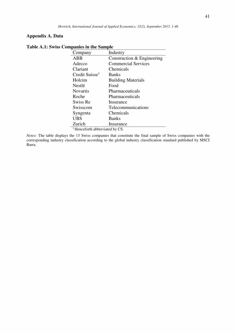
41


Appendix A. Data

Table A.1: Swiss Companies in the Sample

Company Industry

ABB Construction & Engineering

Adecco Commercial Services

Clariant Chemicals

Credit Suisse1 Banks

Holcim Building Materials

Nestlé Food

Novartis Pharmaceuticals

Roche Pharmaceuticals

Swiss Re Insurance

Swisscom Telecommunications

Syngenta Chemicals

UBS Banks

Zurich Insurance 1 Henceforth abbreviated by CS.

Notes: The table displays the 13 Swiss companies that constitute the final sample of Swiss companies with the

corresponding industry classification according to the global industry classification standard published by MSCI

Barra.

42


Table A.2: German Companies in the Sample

Company Industry

Allianz Insurance

BASF Chemicals

Bayer Chemicals

BMW Auto Manufacturers

Commerzbank Banks

Continental Auto Parts & Equipment

Daimler Auto Manufacturers

Deutsche Bank1 Banks

Deutsche Post Transportation

Deutsche Telekom Telecommunications

E.ON Electric

Energie Baden-Württemberg2 Electric

Fresenius Healthcare-Services

Hannover Rück Insurance

HeidelbergCement Building Materials

Henkel Household Products/Wares

Kabel Deutschland Telecommunications

Lanxess Chemicals

Linde Construction & Engineering

Lufthansa Airlines

Merck Pharmaceuticals

Metro Food

Munich Re Insurance

Porsche Auto Manufacturers

ProSiebenSat.1 Media

RWE Electric

Siemens Miscellaneous Manufacturing

Südzucker Food

ThyssenKrupp Iron/Steel

TUI Leisure Time

VW Auto Manufacturers 1 Henceforth abbreviated by DBank. 2 Henceforth abbreviated by EnBW.

Notes: The table displays the 31 German companies that constitute the final sample of German companies with the

corresponding industry classification according to the global industry classification standard published by MSCI

Barra.

43


Appendix B. Univariate Time Series Properties

Table B.1: Stationarity Test for the Bid-Ask Spread and the Mid-Rate

𝐵𝐴𝑆 𝑀𝐼𝐷

ABB 1.84*** 1.59***

Nestlé 2.10*** 3.08***

Roche 1.75*** 2.05***

UBS 1.38*** 1.92***

DBank 1.36*** 2.92***

Merck 1.70*** 1.65***

Siemens 1.75*** 1.81***

VW 1.76*** 2.17***

Notes: The table displays the value of the KPSS test statistic under the null hypothesis that both the bid-ask spread

(𝐵𝐴𝑆) and the mid-rate (𝑀𝐼𝐷) are level stationary for the eight companies in the subsample. The Newey-West

estimator is used to estimate 𝜎2 and the lag truncation parameter is set equal to 3 ∙ √𝑇/13, where 𝑇 is the number of

observations. * / ** / *** denotes significance at the 10%, 5% and 1% significance level, respectively. Data source:

Datastream.

Table B.2: Stationarity Test for the Changes in the Bid-Ask Spread and the Mid-Rate

𝐵𝐴𝑆 𝑀𝐼𝐷

ABB 0.03 0.13

Nestlé 0.03 0.12

Roche 0.04 0.26

UBS 0.03 0.07

DBank 0.02 0.04

Merck 0.05 0.24

Siemens 0.04 0.16

VW 0.04 0.11

Notes: The table displays the value of the KPSS test statistic under the null hypothesis that both the changes in the

bid-ask spread (∆ 𝐵𝐴𝑆) and the mid-rate (∆ 𝑀𝐼𝐷) are level stationary for the eight companies in the subsample. The

Newey-West estimator is used to estimate 𝜎2 and the lag truncation parameter is set equal to 3 ∙ √𝑇/13, where 𝑇 is

the number of observations. * / ** / *** denotes significance at the 10%, 5% and 1% significance level, respectively.

Data source: Datastream.

44


Table B.3: Number of Zero Changes in the Bid-Ask Spread

Total No.

of Zeros

Rel. No. of

Zeros (in %)

ABB 259 35.87

Nestlé 317 43.91

Roche 245 33.93

UBS 237 32.83

DBank 244 33.80

Merck 315 43.63

Siemens 308 42.66

VW 208 28.81

Notes: The table displays the total number (No.) of zero changes in the bid-ask spread (column 2) and the same

number relative (Rel.) to the total number of observations (column 3) for the eight companies in the subsample. Data

source: Datastream.

Table B.4: Autocorrelation Test for the Changes in the Bid-Ask Spread and the Mid-Rate

∆𝐵𝐴𝑆 ∆𝑀𝐼𝐷

ABB 186.80*** 52.88***

Nestlé 123.20*** 32.17***

Roche 134.30*** 61.12***

UBS 139.40*** 86.16***

DBank 125.80*** 62.35***

Merck 116.70*** 82.75***

Siemens 113.60*** 35.82***

VW 183.60*** 78.03***

Notes: The table displays the value of the Ljung-Box test statistic under the null hypothesis that both the changes in

the bid-ask spread (∆𝐵𝐴𝑆) and the mid-rate (∆𝑀𝐼𝐷) are serially uncorrelated for the eight companies in the

subsample. * / ** / *** denotes significance at the 10%, 5% and 1% significance level, respectively. Data source:

Datastream.

45


Appendix C. Empirical Results with Exogenous Variables

Table C.1: Exogenous Explanatory Variables and Expected Sign

Variable Description Sign ∆𝐵𝐴𝑆 Sign ∆𝑀𝐼𝐷 𝑟𝑡𝑓 Risk-Free Rate + - 𝑟𝑡 Stock Returns - - 𝜎𝑡30 Historical Stock Volatility (30 Days) + + 𝜎𝑡360 Historical Stock Volatility (360 Days) + + 𝜎𝑡𝑖𝑚𝑝

Option-Implied Volatility (Stock) + + 𝑠𝑙𝑡 Slope of the Yield Curve - - 𝑡𝑒𝑑𝑡 TED Spread + + 𝑑𝑠𝑝𝑟𝑒𝑎𝑑𝑡 Default Yield Spread + + 𝑟𝑚,𝑡 Stock Market Returns - - 𝑣𝑑𝑎𝑥𝑡 Option-Implied Volatility (DAX) + + 𝑑𝑦𝑡 Dividend Yield n.a. - 𝑝𝑏𝑡 Price-to-Book Ratio n.a. - 𝑟𝑠𝑖𝑡 Short-Term Momentum n.a. n.a. 𝑟𝑚𝑜𝑚𝑡 Long-Term Momentum n.a. n.a.

Notes: The table displays the expected sign for the impact of the used exogenous explanatory variables (column 1,

"Variable") on the changes of both the CDS bid-ask spread (column 3, "Sign ∆𝐵𝐴𝑆") and the CDS mid-rate (column

4, "Sign ∆𝑀𝐼𝐷"), respectively, assuming that the corresponding exogenous variable rises. Rows with a "n.a." value

denote the cases, where the expected sign is ambiguous. In the column 2 ("Description"), the exogenous variables

are briefly explained.

Table C.2: Granger Causality Test for the Swiss Companies with Exogenous Variables


ABB 0.391 0.768

Adecco 1.402 1.227

Clariant 0.904 2.137*

CS 0.704 1.876*

Holcim 1.492 2.926***

Nestlé 1.101 0.826

Novartis 0.933 0.902

Roche 0.232 6.884***

Swisscom 0.855 1.944*

SwissRe 1.796* 2.106**

Syngenta 0.778 0.628

UBS 1.451 1.181

Zurich 1.210 1.694

Notes: The table displays the value of the F-test statistic of the Granger causality test in the bivariate 𝑉𝐴𝑅𝑋(𝑝) for

the null hypothesis that changes in the bid-ask spread do not Granger-cause changes in the mid-rate

(∆𝐵𝐴𝑆 𝐺𝑟𝐶⇏ ∆𝑀𝐼𝐷) and vice versa (∆𝑀𝐼𝐷 𝐺𝑟𝐶⇏ ∆𝐵𝐴𝑆) for the 13 Swiss companies in the sample. * / ** / *** denotes

significance at the 10%, 5% and 1% significance level, respectively. Data source: Bloomberg, Datastream.

46


Table C.3: Granger Causality Test for the German Companies with Exogenous Variables


Allianz 1.010 1.794*

BASF 0.670 0.171

Bayer 2.153* 1.509

BMW 1.065 1.123

Commerzbank 0.843 2.672**

Continental 2.092* 2.513**

Daimler 0.348 1.454

DBank 0.437 1.545

DPost 0.700 1.929*

DTelekom 0.507 1.287

EnBW 1.377 1.352

E.ON 0.792 2.475**

Fresenius 2.341** 4.037***

HannoverRück 1.379 2.416**

HeidelbergCement 0.726 0.508

Henkel 1.388 1.271

Lanxess 0.250 1.265

Linde 1.710 1.576

Lufthansa 0.936 1.678

Merck 1.166 1.489

Metro 0.991 1.871*

Munich Re 2.218* 2.645**

Porsche 1.049 1.597

ProSiebenSat.1 1.590 0.933

RWE 1.706 1.959*

Siemens 0.390 1.876*

Südzucker 0.563 1.192

ThyssenKrupp 0.599 3.842***

TUI 0.718 2.208**

VW 0.496 2.345**

Notes: The table displays the value of the F-test statistic of the Granger causality test in the bivariate 𝑉𝐴𝑅𝑋(𝑝) for

the null hypothesis that changes in the bid-ask spread do not Granger-cause changes in the mid-rate

(∆𝐵𝐴𝑆 𝐺𝑟𝐶⇏ ∆𝑀𝐼𝐷) and vice versa (∆𝑀𝐼𝐷 𝐺𝑟𝐶⇏ ∆𝐵𝐴𝑆) for the 31 German companies in the sample. * / ** / *** denotes

significance at the 10%, 5% and 1% significance level, respectively. Data source: Bloomberg, Datastream.

Does Credit Risk Impact Liquidity Risk? Evidence from Credit ...

Documents