Cranfield University Panagiotis Giannakakis Design space ...

Cranfield University

Panagiotis Giannakakis

Design space exploration and

performance modelling of advanced

turbofan and open-rotor engines

SCHOOL OF ENGINEERING

EngD Thesis

Cranfield University

School of Engineering

EngD Thesis

2013

Panagiotis Giannakakis

Design space exploration and performance

modelling of advanced turbofan and

open-rotor engines

Supervisor: Dr. P. Laskaridis & Prof. R. Singh

This thesis is submitted in partial fullfillment of the requirements for the

degree of Doctor of Engineering

c©Cranfield University, 2013. All rights reserved. No part of this

publication my be reproduced without written permission of the

copyright holder.

This work is dedicated to

all the members of my family,

and to my patient Marie.

Acknowledgements

First of all, I would like to thank my supervisor Dr. Panagiotis Laskaridis for

all the time, ideas and effort he has put in my project. Our long discussions

instigated many of the themes presented here.

I would like to express my gratitude to Prof. Riti Singh for providing his

insightful views throughout the course of this project. I also wish to thank

Prof. Pericles Pilidis for teaching me gas turbine performance, for his trust

and his advice in technical and personal level.

The financial support of the Boeing Commercial Aircraft Company and the

invaluable advice of its engineers are gratefully acknowledged.

I am very thankful to Prof. Anestis Kalfas, who was always there to support,

advise and motivate me. I wish to extend my gratitude to all the teachers that

inspired and shaped me as an engineer and person throughout my studies.

Special thanks to all the staff of the Cranfield University Library for providing

us with such a high quality of services. Thanks are also due to all the staff

of the Department of Power and Propulsion for their valuable services and

support.

Thanks are due to Konstantinos Kyprianidis for our interesting and stimulat-

ing discussions on the topics of engine performance, simulation and prelimi-

nary design. I owe a lot to Periklis Lolis, who provided his preliminary design

and weight code, and dedicated a lot of time and patience to help me realise

the turbofan design exploration study. The propeller part of this thesis would

not exist without the invaluable contributions of Georgios Iosifidis and Ioannis

Goulos, who embarked with me in this exciting trip in the fundamentals of

propeller aerodynamics. I would also like to thank Jan Janikovic, Georgios

Doulgeris and Theoklis Nikolaidis for our fruitful and interesting interactions,

within the code development activities of the department.

I had the chance to work with many MSc students and gain through them

much experience and knowledge. Many thanks to Egoitz Rodriguez, Chinmay

Beura, Iker Manzanedo, Devaiah Nalianda, Benjamin Bruni, Alfonso Ortal

Sevilla, Ilektra Kanaki, Jessica Gridel, Alicia Sanchez-Ortega and Steve Owen.

Many thanks to my colleagues Devaiah, Domenico, Eduardo and my tolerant

officemate Alice, for sharing our thoughts and worries, and for making this

personal research journey a bit less lonely.

I owe my fullest gratitude to my housemates Pavlos, Alekos, Peri, Giorgos

and Fanis for being a real family to me and for all the moments we shared

together. A big thank you to my friends in Cranfield, Asteris, Avgoustinos,

Elias and Yiannis for lightening up my life there and for giving me so many

nice memories. Because of my housemates and friends I will always think

about the time in Cranfield in a sweet nostalgic tone.

I am deeply grateful to my old friends Sotos, Dionysis, Alexandros, Apostolis,

and Teo for honouring me all these years with their support, camaraderie and

care.

Finally, special thanks to my colleagues in YYPV, Snecma, for their warm

welcome and for their understanding during the writing up of this thesis.

Abstract

This work focuses on the current civil engine design practice of increasing overall pres-

sure ratio, turbine entry temperature and bypass ratio, and on the technologies required in

order to sustain it. In this context, this thesis contributes towards clarifying the following

gray aspects of future civil engine development:

• the connection between an aircraft application, the engine thermodynamic cycle and

the advanced technologies of variable area fan nozzle and fan drive gearbox.

• the connection between the engine thermodynamic cycle and the fuel consumption

penalties of extracting bleed or power in order to satisfy the aircraft needs.

• the scaling of propeller maps in order to enable extensive open-rotor studies similar

to the ones carried out for turbofan engines.

The first two objectives are tackled by implementing a preliminary design framework,

which comprises models that calculate the engine uninstalled performance, dimensions,

weight, drag and installed performance. The framework produces designs that are in

good agreement with current and near future civil engines. The need for a variable area

fan nozzle is related to the fan surge margin at take-off, while the transition to a geared

architecture is identified by tracking the variation of the low pressure turbine number of

stages. The results show that the above enabling technologies will be prioritised for long

range engines, due to their higher overall pressure ratio, higher bypass ratio and lower

specific thrust. The analysis also shows that future lower specific thrust engines will suffer

from higher secondary power extraction penalties.

A propeller modelling and optimisation method is created in order to accomplish the

open-rotor aspect of this work. The propeller model follows the lifting-line approach and

is found to perform well against experimental data available for the SR3 prop-fan. The

model is used in order to predict the performance of propellers with the same distribution

of airfoils and sweep, but with different design point power coefficient and advance ratio.

The results demonstrate that all the investigated propellers can be modelled by a common

map, which separately determines the ideal and viscous losses.

i

ii

Contents

Abstract i

Table of Contents ii

List of Figures vi

List of Tables xiii

Nomenclature xiii

1 Introduction 1

1.1 Research scope . . . . . . . . . . . . . . . . . . . . . . . . . . . . . . . . . 1

1.2 Literature overview . . . . . . . . . . . . . . . . . . . . . . . . . . . . . . . 2

1.2.1 Variable area fan nozzle . . . . . . . . . . . . . . . . . . . . . . . . 2

1.2.2 Geared turbofan architecture . . . . . . . . . . . . . . . . . . . . . 2

1.2.3 More electric technologies . . . . . . . . . . . . . . . . . . . . . . . 2

1.2.4 Open-rotor configuration . . . . . . . . . . . . . . . . . . . . . . . . 3

1.3 Project aim and objectives . . . . . . . . . . . . . . . . . . . . . . . . . . . 4

1.4 Thesis structure . . . . . . . . . . . . . . . . . . . . . . . . . . . . . . . . . 4

2 Advanced turbofan design space exploration 7

2.1 Introduction . . . . . . . . . . . . . . . . . . . . . . . . . . . . . . . . . . . 7

2.2 Engine Efficiency Fundamentals . . . . . . . . . . . . . . . . . . . . . . . . 8

2.3 Low pressure system enabling technologies . . . . . . . . . . . . . . . . . . 13

2.4 Numerical methods and models used . . . . . . . . . . . . . . . . . . . . . 15

2.4.1 Engine model - TURBOMATCH . . . . . . . . . . . . . . . . . . . 15

2.4.2 Engine preliminary design and weight estimation tool . . . . . . . . 17

2.4.3 Installed performance calculation . . . . . . . . . . . . . . . . . . . 17

2.4.4 Optimisation method . . . . . . . . . . . . . . . . . . . . . . . . . . 19

2.5 Engine design principles . . . . . . . . . . . . . . . . . . . . . . . . . . . . 19

2.6 Engine thermodynamic design approach . . . . . . . . . . . . . . . . . . . 21

iii

2.7 Uninstalled performance study . . . . . . . . . . . . . . . . . . . . . . . . . 23

2.7.1 Model configuration and assumptions . . . . . . . . . . . . . . . . . 23

2.7.2 Uninstalled performance results . . . . . . . . . . . . . . . . . . . . 24

2.7.2.1 The TET ratio between take-off and climb . . . . . . . . . 29

2.7.2.2 Design space limits for the selection of OPR . . . . . . . . 30

2.8 LP system enabling technologies study . . . . . . . . . . . . . . . . . . . . 33

2.8.1 Variable area fan nozzle . . . . . . . . . . . . . . . . . . . . . . . . 33

2.8.2 Gearbox study . . . . . . . . . . . . . . . . . . . . . . . . . . . . . 34

2.8.2.1 Design assumptions . . . . . . . . . . . . . . . . . . . . . 34

2.8.2.2 Gearbox baseline results . . . . . . . . . . . . . . . . . . . 37

2.8.2.3 The effect of component efficiencies . . . . . . . . . . . . . 41

2.8.2.4 The effect of OPR . . . . . . . . . . . . . . . . . . . . . . 42

2.9 Installed performance results . . . . . . . . . . . . . . . . . . . . . . . . . . 44

2.9.1 Validation . . . . . . . . . . . . . . . . . . . . . . . . . . . . . . . . 45

2.9.2 Optimum specific thrust . . . . . . . . . . . . . . . . . . . . . . . . 45

2.9.3 TET limitation . . . . . . . . . . . . . . . . . . . . . . . . . . . . . 46

2.9.4 HPC delivery temperature limitation . . . . . . . . . . . . . . . . . 46

2.9.5 Variable area fan nozzle . . . . . . . . . . . . . . . . . . . . . . . . 47

2.9.6 Gearbox . . . . . . . . . . . . . . . . . . . . . . . . . . . . . . . . . 47

2.9.7 Exchange rates . . . . . . . . . . . . . . . . . . . . . . . . . . . . . 48

2.9.7.1 Overall pressure ratio . . . . . . . . . . . . . . . . . . . . 49

2.9.7.2 Turbine entry temperature and Variable area fan nozzle . 49

2.9.7.3 Improved installation technology and lower specific thrust 50

2.9.8 Some possible design paths . . . . . . . . . . . . . . . . . . . . . . . 51

2.9.8.1 Short range engine . . . . . . . . . . . . . . . . . . . . . . 51

2.9.8.2 Long range engine . . . . . . . . . . . . . . . . . . . . . . 51

2.10 Conclusions . . . . . . . . . . . . . . . . . . . . . . . . . . . . . . . . . . . 52

3 Secondary power extraction effects 59

3.1 Introduction . . . . . . . . . . . . . . . . . . . . . . . . . . . . . . . . . . . 59

3.2 Engine Core Efficiency Analysis . . . . . . . . . . . . . . . . . . . . . . . . 60

3.2.1 Shaft power off-takes . . . . . . . . . . . . . . . . . . . . . . . . . . 61

3.2.2 Bleed air off-takes . . . . . . . . . . . . . . . . . . . . . . . . . . . . 62

3.3 Engine Total Efficiency Analysis . . . . . . . . . . . . . . . . . . . . . . . . 63

3.3.1 Constant Specific Thrust . . . . . . . . . . . . . . . . . . . . . . . . 63

3.3.2 Constant Bypass Ratio . . . . . . . . . . . . . . . . . . . . . . . . . 64

3.4 Validation . . . . . . . . . . . . . . . . . . . . . . . . . . . . . . . . . . . . 65

3.5 Future Engines Penalties . . . . . . . . . . . . . . . . . . . . . . . . . . . . 69

3.6 Resizing Methods Comparison . . . . . . . . . . . . . . . . . . . . . . . . . 72

iv

3.7 Conclusions . . . . . . . . . . . . . . . . . . . . . . . . . . . . . . . . . . . 74

4 Propeller modelling method development 77

4.1 Introduction . . . . . . . . . . . . . . . . . . . . . . . . . . . . . . . . . . . 77

4.2 Propeller fundamentals . . . . . . . . . . . . . . . . . . . . . . . . . . . . . 77

4.3 Analysis methods . . . . . . . . . . . . . . . . . . . . . . . . . . . . . . . . 79

4.4 Lifting-line method development . . . . . . . . . . . . . . . . . . . . . . . . 81

4.4.1 Coordinate systems . . . . . . . . . . . . . . . . . . . . . . . . . . . 81

4.4.2 Blade-element velocity analysis . . . . . . . . . . . . . . . . . . . . 84

4.4.3 Wake geometry definition . . . . . . . . . . . . . . . . . . . . . . . 86

4.4.4 Biot-Savart law . . . . . . . . . . . . . . . . . . . . . . . . . . . . . 88

4.4.5 Vortex induced velocity calculation . . . . . . . . . . . . . . . . . . 90

4.4.6 Calculation of circulation . . . . . . . . . . . . . . . . . . . . . . . . 92

4.4.7 Blade-element performance . . . . . . . . . . . . . . . . . . . . . . . 97

4.4.8 Compressibility effects . . . . . . . . . . . . . . . . . . . . . . . . . 100

4.5 Method verification and validation . . . . . . . . . . . . . . . . . . . . . . 104

4.5.1 Case description . . . . . . . . . . . . . . . . . . . . . . . . . . . . . 104

4.5.2 Model configuration . . . . . . . . . . . . . . . . . . . . . . . . . . 106

4.5.3 Results . . . . . . . . . . . . . . . . . . . . . . . . . . . . . . . . . . 108

4.6 Conclusions . . . . . . . . . . . . . . . . . . . . . . . . . . . . . . . . . . . 116

5 The development of a scalable propeller map representation 119

5.1 Introduction . . . . . . . . . . . . . . . . . . . . . . . . . . . . . . . . . . . 119

5.2 Propeller map scaling literature . . . . . . . . . . . . . . . . . . . . . . . . 120

5.3 SR3 prop-fan map . . . . . . . . . . . . . . . . . . . . . . . . . . . . . . . 122

5.3.1 The Mach number effect . . . . . . . . . . . . . . . . . . . . . . . . 126

5.4 Design and optimisation . . . . . . . . . . . . . . . . . . . . . . . . . . . . 130

5.4.1 The propeller design problem . . . . . . . . . . . . . . . . . . . . . 130

5.4.2 Method selection . . . . . . . . . . . . . . . . . . . . . . . . . . . . 130

5.4.3 Optimisation problem formulation . . . . . . . . . . . . . . . . . . . 132

5.4.4 Optimisation results . . . . . . . . . . . . . . . . . . . . . . . . . . 134

5.4.4.1 Step 1: optimise twist and pitch with constant chord . . . 134

5.4.4.2 Step 2: optimise twist, pitch and chord . . . . . . . . . . . 135

5.5 Results analysis to devise a map scaling technique . . . . . . . . . . . . . . 138

5.5.1 Step 1: optimise twist and pitch with constant chord . . . . . . . . 140

5.5.2 Step 2: optimise twist, pitch and chord . . . . . . . . . . . . . . . . 141

5.5.3 The Mach number effect for different designs . . . . . . . . . . . . . 143

5.5.4 Discussion . . . . . . . . . . . . . . . . . . . . . . . . . . . . . . . . 148

5.6 Conclusions . . . . . . . . . . . . . . . . . . . . . . . . . . . . . . . . . . . 150

v

6 Conclusions & Future work 153

6.1 Summarising the key elements . . . . . . . . . . . . . . . . . . . . . . . . . 153

6.1.1 Advanced turbofan design space exploration . . . . . . . . . . . . . 153

6.1.2 Secondary power extraction effects . . . . . . . . . . . . . . . . . . 156

6.1.3 Propeller modelling method development . . . . . . . . . . . . . . . 158

6.1.4 The development of a scalable propeller map representation . . . . 159

6.2 Author’s contribution . . . . . . . . . . . . . . . . . . . . . . . . . . . . . . 161

6.3 Future work . . . . . . . . . . . . . . . . . . . . . . . . . . . . . . . . . . . 163

References 165

vi

List of Figures

2.1 Schematic representation of a turbofan engine. The main power conversions

are also shown. The term core power describes the mainstream product

of the core, while the secondary power extraction consists of bleed air and

shaft power. . . . . . . . . . . . . . . . . . . . . . . . . . . . . . . . . . . . 8

2.2 Variation of transmission efficiency with bypass ratio, fan and turbine effi-

ciency. . . . . . . . . . . . . . . . . . . . . . . . . . . . . . . . . . . . . . . 10

2.3 Variation of propulsive efficiency with specific thrust. . . . . . . . . . . . . 11

2.4 Engine schematic showing the definition of nacelle dimensions . . . . . . . 18

2.5 Engine configuration schematic showing the definition of OPR, T3 and

TET. The bypass and core nozzles are designated by BPN and CN re-

spectively. . . . . . . . . . . . . . . . . . . . . . . . . . . . . . . . . . . . 23

2.6 Baseline uninstalled SFC design map, also showing the variation of opti-

mum FPR (white lines). . . . . . . . . . . . . . . . . . . . . . . . . . . . . 25

2.7 The effect of OPR and component efficiencies on the optimum value of FPR. 27

2.8 The relation between specific thrust (ST) and FPR (η = 90% OPR = 30).

The plotted points represent results for the full range of TET and BPR. . . 28

2.9 The uninstalled SFC design map, using the specific thrust as a design

parameter. . . . . . . . . . . . . . . . . . . . . . . . . . . . . . . . . . . . . 29

2.10 The relation between specific thrust (ST) and the ratio of TET between

ToC and TO. The plotted points represent results for the full range of TET

and BPR. . . . . . . . . . . . . . . . . . . . . . . . . . . . . . . . . . . . . 30

2.11 The effect of specific thrust (through the definition of TET and BPR) on

the location of the TO point on the fan map (η = 90% OPR = 30). . . . . 31

2.12 The effect of component efficiencies and OPR on the maximum T3 and on

the uninstalled SFC. One continuous line for each increased level of OPR

splits the design space in the right region where there is an SFC benefit

and in the left where the SFC deteriorates. SFC benefit relative to OPR=30. 32

2.13 The relation between OPR, specific thrust, component efficiencies and max-

imum T3. The plotted points represent results for the full range of TET

and BPR. . . . . . . . . . . . . . . . . . . . . . . . . . . . . . . . . . . . . 32

vii

2.14 (a) The relation between FPR and the surge margin parameter for different

component efficiencies and OPR, for the full range of TET and BPR. (b)

The impact of varying the fan nozzle area at take-off on the fan surge

margin parameter. (c) The required fan nozzle area increase at take-off in

order to keep a safe fan margin. The results by Jackson can be found in

[17]. (d) The impact of the fan nozzle area increase on the ratio of TET at

take-off to the TET at mid-cruise. . . . . . . . . . . . . . . . . . . . . . . . 35

2.15 The relation between TET, BPR and the number of LPT stages (η =

85% OPR = 30). . . . . . . . . . . . . . . . . . . . . . . . . . . . . . . . . 37

2.16 The relation between TET, BPR and the LPT enthalpy drop as predicted

by the simulation framework and by the equation (η = 85% OPR = 30). . 39

2.17 The relation between TET, BPR and the LPT mean blade speed as pre-

dicted by the equation for a constant density term or by the simulation

framework with a real varying density term (η = 85% OPR = 30). . . . . . 41

2.18 The effect of increased component efficiency on the number of stages (OPR

= 30). . . . . . . . . . . . . . . . . . . . . . . . . . . . . . . . . . . . . . . 42

2.19 The effect of increased OPR on the LPT enthalpy drop and mean blade

speed (η = 85%). . . . . . . . . . . . . . . . . . . . . . . . . . . . . . . . . 43

2.20 The effect of increased OPR on the number of stages (η = 85%). . . . . . . 43

2.21 The short range design map for different OPR and component efficiencies.

Square: baseline optimum. Diamond: increased TET optimum. Circle:

Geared increased TET optimum. Continuous lines: iso ST [m/s] at ToC.

Dotted lines: iso number of LPT stages. Dash-dot lines: iso TET [K] at TO. 55

2.22 The long range design map for different OPR and component efficiencies.

Square: baseline optimum. Diamond: increased TET optimum. Triangle:

Geared optimum. Circle: Geared increased TET optimum. Continuous

lines: iso ST [m/s] at ToC. Dotted lines: iso number of LPT stages. Dash-

dot lines: iso TET [K] at TO. . . . . . . . . . . . . . . . . . . . . . . . . . 56

2.23 The relation between the specific thrust and the fan tip diameter for the

short and long range engine (η = 90% OPR = 40). . . . . . . . . . . . . . 57

2.24 SFC and range factor (K) exchange rates for different missions and com-

ponent efficiencies. The short and long range mission baseline engines

correspond to the square symbols of Fig. 2.21a and Fig. 2.22a respectively.

The low weight and drag case corresponds to: -50% drag and -35% weight

for the SR and -45% for the LR. . . . . . . . . . . . . . . . . . . . . . . . . 58

3.1 Enthalpy-entropy diagram at the core exit with and without off-takes. . . . 61

viii

3.2 Variation of shaft power off-take penalties with bypass ratio. Resizing with

constant bypass ratio. Shaft power extracted from the HP spool. TET =

1650 [K]. Predictions made with Eq. 3.6 and Eq. 3.19. . . . . . . . . . . . 66

3.3 Variation of bleed air penalties with bypass ratio. Resizing with constant

bypass ratio. Bleed air extracted from the HPC delivery. TET = 1650 [K].

Predictions made with Eq. 3.13 and Eq. 3.19. . . . . . . . . . . . . . . . . 66

3.4 Variation of shaft power off-take penalties with specific thrust. Resizing

with constant specific thrust. Shaft power extracted from the HP spool.

TET = 1650 [K]. Predictions made with Eq. 3.6 and Eq. 3.17. . . . . . . . 67

3.5 Variation of bleed air penalties with specific thrust. Resizing with constant

specific thrust. Bleed air extracted from the HPC delivery. TET = 1650

[K]. Predictions made with Eq. 3.13 and Eq. 3.17. . . . . . . . . . . . . . . 67

3.6 Installed SFC prediction error throughout the whole range of BPR and

TET. Resizing with constant bypass ratio. 0.85 [kg/s] bleed air extracted

from the HPC delivery. The term installed SFC includes only the secondary

power extraction penalty; no other installation effect is included. . . . . . . 68

3.7 SFC penalty prediction throughout the whole range of Specific Thrust and

TET. Resizing with constant bypass ratio. 500 [kW] of shaft power ex-

tracted from the HP spool. . . . . . . . . . . . . . . . . . . . . . . . . . . . 70

3.8 SFC penalty prediction of Eq. 3.19 and Eq. 3.6 for different specific thrusts

and non-dimensional power factors. Resizing with constant bypass ratio.

Shaft power extracted from the HP spool. BPR = 6. . . . . . . . . . . . . 71

3.9 Propulsive efficiency gain when resizing with constant bypass ratio. 500

[kW] of shaft power extracted from the HP spool. . . . . . . . . . . . . . . 72

3.10 Transmission efficiency gain when resizing with constant specific thrust.

500 [kW] of shaft power extracted from the HP spool. . . . . . . . . . . . . 73

3.11 SFC benefit of engine resizing with constant bypass ratio relative to the

constant specific thrust method. 500 [kW] of shaft power extracted from

the HP spool. . . . . . . . . . . . . . . . . . . . . . . . . . . . . . . . . . . 74

4.1 Coordinate systems used. XY Z: global cartesian system. rφZ: global

cylindrical system. scn: local blade-element system. V0: flight velocity. Ω:

propeller rotational speed. . . . . . . . . . . . . . . . . . . . . . . . . . . . 82

4.2 Local blade element coordinate system in the cn plane. s: spanwise unit

vector. c: chordwise unit vector. n: normalwise unit vector . . . . . . . . . 82

4.3 Panair input and output data. . . . . . . . . . . . . . . . . . . . . . . . . . 85

4.4 The modelling of the blade with a bound vortex and of the wake with a set

of trailing vortex filaments. . . . . . . . . . . . . . . . . . . . . . . . . . . . 87

4.5 The resulting non-contracted prescribed wake geometry. . . . . . . . . . . . 88

ix

4.6 The Biot-Savart law, giving the velocity ~w induced by a straight vortex

segment ~lAB with a finite core radius as given by Leishman [127]. . . . . . 89

4.7 The discretisation of the blade and the wake. The blade is depicted with

grey background. . . . . . . . . . . . . . . . . . . . . . . . . . . . . . . . . 90

4.8 The relation between bound and trailing vortex circulation. . . . . . . . . . 91

4.9 Blade-element aerodynamic performance described by the flow velocity in

the cn plane and the lift and drag forces. . . . . . . . . . . . . . . . . . . . 94

4.10 Overview of the blade circulation calculation process. . . . . . . . . . . . . 97

4.11 Efficiency prediction results from Rohrbach et al [105] using the Borst

corrections. Prediction for the SR3 propeller, J = 3.06 and CP = 1.695.

Unrealistic change of curvature after Mach = 0.80. . . . . . . . . . . . . . . 102

4.12 The SR3 blade/spinner/nacelle geometry as reconstructed by the developed

code. . . . . . . . . . . . . . . . . . . . . . . . . . . . . . . . . . . . . . . . 106

4.13 Grid independency study for the propeller modelling parameters. Operat-

ing conditions: M=0.8, J=3.06, Pitch=58.50. All parameters are set to

the values of table 4.4. . . . . . . . . . . . . . . . . . . . . . . . . . . . . . 109

4.14 Grid independency study for the nacelle/spinner modelling parameters.

Operating conditions: M=0.8, J=3.06, Pitch=58.50. All parameters are

set to the values of table 4.4. . . . . . . . . . . . . . . . . . . . . . . . . . . 110

4.15 The SR3 blade/spinner/nacelle/wake grid as discretised by the developed

code according to the settings given in table 4.4. . . . . . . . . . . . . . . . 110

4.16 The effect of blade deformations on the power coefficient and efficiency. . . 111

4.17 The effect of Mach number on the lift coefficient CL for the NACA-16-204

airfoil. . . . . . . . . . . . . . . . . . . . . . . . . . . . . . . . . . . . . . . 112

4.18 Comparison of Mach number profile predicted by PAN AIR with test data

extracted from Egolf et al [117]. Measurements taken at plane Z/Lref =

0.09 for Mref=0.8. Lref=12.25 inches. . . . . . . . . . . . . . . . . . . . . . 112

4.19 Validation of the power coefficient and efficiency predicted by the lifting-

line method against experimental data extracted from Stefko and Jeracki

[148] for M=0.2. . . . . . . . . . . . . . . . . . . . . . . . . . . . . . . . . . 114

4.20 Validation of the power coefficient and efficiency predicted by the lifting-

line method against experimental data extracted from Jeracki et al [150]

for M=0.6. . . . . . . . . . . . . . . . . . . . . . . . . . . . . . . . . . . . . 115

4.21 Validation of the power coefficient predicted by the lifting-line method

against experimental data extracted from Rohrbach et al [105] for M=0.8.

The predictions by Hanson et al [83] have also been added as a comparison

base. . . . . . . . . . . . . . . . . . . . . . . . . . . . . . . . . . . . . . . . 115

x

4.22 Validation against the ideal efficiency and measured real efficiency quoted

by Jeracki et al [150]. The no-induced prediction represents the predicted

efficiency if the induced velocities are set to zero. The ideal efficiency

represents the efficiency with zero drag. CP=1.7, J=3.06. . . . . . . . . . . 116

5.1 A full performance map for the SR3 propeller at low speed conditions

M=0.2. The contours represent the real or ideal efficiency, while the iso-

pitch-angle lines are depicted in dashed style. . . . . . . . . . . . . . . . . 123

5.2 The variation of the angle of attack at the 3/4 blade radius for the SR3

propeller at low speed conditions M=0.2. The angles are in degrees, while

the iso-pitch-angle lines are depicted in dashed style. . . . . . . . . . . . . 124

5.3 Simplified blade element performance. The schematic assumes a straight

blade with zero induced velocities, zero drag and no effect of nacelle. . . . . 125

5.4 An alternative CT performance map for the SR3 propeller at low speed

conditions M=0.2. The contours represent the thrust coefficient, while the

iso-pitch-angle lines are depicted in dashed style. . . . . . . . . . . . . . . . 126

5.5 A full performance map for the SR3 propeller at high speed conditions

M=0.6-0.8. The contours represent the efficiency, while the iso-pitch-angle

lines are depicted in dashed style. . . . . . . . . . . . . . . . . . . . . . . . 127

5.6 The effect of flight Mach number on propeller efficiency for different oper-

ating power advance ratios and power coefficients. . . . . . . . . . . . . . . 128

5.7 The variation of helical mach number at the 3/4 of the blade radius for

different flight mach numbers and advance ratios. . . . . . . . . . . . . . . 129

5.8 The variation of relative efficiency with helical mach number at 0.75R for

different operating advance ratios and power coefficients. The relative effi-

ciency is defined as the efficiency divided by the maximum efficiency for a

given advance ratio and power coefficient. . . . . . . . . . . . . . . . . . . 129

5.9 The optimum distribution of twist for different design advance ratios J .

The blade chord distribution is held constant. Design Mach number equal

to 0.8. . . . . . . . . . . . . . . . . . . . . . . . . . . . . . . . . . . . . . . 136

5.10 The change in the lift coefficient distribution for different design power

coefficients CP and advance ratios J . The blade chord distribution is held

constant. Design Mach number equal to 0.8. . . . . . . . . . . . . . . . . . 136

5.11 The change in the propeller efficiency for different design power coefficients

CP and advance ratios J . The blade chord distribution is held constant.

Design Mach number equal to 0.8. . . . . . . . . . . . . . . . . . . . . . . . 137

5.12 The optimum distribution of twist and chord for different design CP and

J . The blade chord distribution is optimised. Design Mach number equal

to 0.8. . . . . . . . . . . . . . . . . . . . . . . . . . . . . . . . . . . . . . . 139

xi

5.13 The change in the lift coefficient distribution for different design CP and

J . The blade chord distribution is optimised. Design Mach number equal

to 0.8. . . . . . . . . . . . . . . . . . . . . . . . . . . . . . . . . . . . . . . 139

5.14 The change in the propeller efficiency for different design power coefficients

CP and advance ratios J . The blade chord distribution is optimised. Design

Mach number equal to 0.8. . . . . . . . . . . . . . . . . . . . . . . . . . . . 140

5.15 The change in the ideal efficiency and viscous losses map for different design

power coefficients CP . The blade chord distribution is held constant. Mach

= 0.2. . . . . . . . . . . . . . . . . . . . . . . . . . . . . . . . . . . . . . . 141

5.16 The variation of the efficiency map, for different design power coefficients

CP and advance ratios J . The blade chord distribution is held constant.

Mach = 0.2. . . . . . . . . . . . . . . . . . . . . . . . . . . . . . . . . . . . 142

5.17 The change in the ideal efficiency and viscous losses map for different design

power coefficients CP . The blade chord distribution is optimised. Mach =

0.2. . . . . . . . . . . . . . . . . . . . . . . . . . . . . . . . . . . . . . . . . 143

5.18 The variation of the lift coefficient in the relative coordinates map, for

different design power coefficients CP . The map uses the CL at the 0.75R

point as typical of the blade performance. The blade chord distribution is

optimal. Mach = 0.2. . . . . . . . . . . . . . . . . . . . . . . . . . . . . . . 144

5.19 The variation of viscous losses as a function of the operating [email protected]

and the operating advance ratio, for different design power coefficients CP .

The blade chord distribution is optimal. Mach = 0.2. . . . . . . . . . . . . 144

5.20 The variation of CL and the viscous losses in the relative coordinates map,

for different design power coefficients CP . The blade chord distribution is

optimal. Mach = 0.2. . . . . . . . . . . . . . . . . . . . . . . . . . . . . . . 145

5.21 The scalable ideal efficiency and viscous losses maps for the SR3 prop-fan.

Mach = 0.2. . . . . . . . . . . . . . . . . . . . . . . . . . . . . . . . . . . . 145

5.22 The mach number correction curve for four different design conditions.

Each propeller operates at the design power coefficient and advance ratio.

The twist and chord are optimal. . . . . . . . . . . . . . . . . . . . . . . . 147

5.23 The effect of the operating CL on the mach number correction curve.

The CL at the 0.75R is used. The CPdes = 1.13 propeller operates at

(CP = 1.58, J = 2.80), while the CPdes = 1.70 propeller operates at

(CP = 2.72, J = 2.89). The CL = 0.36 curve represents the results of

Fig. 5.22. The twist and chord of each design are optimal. . . . . . . . . . 147

5.24 The change of the relative efficiency contours plotted using the relative CPand J for two different design power coefficients. The relative efficiency is

defined as the efficiency of each point divided by the maximum efficiency

of the map. . . . . . . . . . . . . . . . . . . . . . . . . . . . . . . . . . . . 149

xii

List of Tables

2.1 Engine thermodynamic specifications . . . . . . . . . . . . . . . . . . . . . 24

2.2 Basic preliminary design code assumptions . . . . . . . . . . . . . . . . . . 36

2.3 Installed performance calculation assumptions . . . . . . . . . . . . . . . . 44

2.4 Low weight and drag case assumptions . . . . . . . . . . . . . . . . . . . . 44

2.5 Range factor engine parameters exchange rates . . . . . . . . . . . . . . . . 57

3.1 Engine specifications . . . . . . . . . . . . . . . . . . . . . . . . . . . . . . 65

4.1 SR3 blade geometry definition. Source: Rohrbach et al [105]. . . . . . . . . 104

4.2 SR3 spinner geometry definition. Rref = 0.1105. Source: Stefko and

Jeracki [148]. . . . . . . . . . . . . . . . . . . . . . . . . . . . . . . . . . . 105

4.3 SR3 nacelle geometry definition. Rref = 0.1105. Source: Stefko and Jeracki

[148]. . . . . . . . . . . . . . . . . . . . . . . . . . . . . . . . . . . . . . . . 105

4.4 Model configuration. . . . . . . . . . . . . . . . . . . . . . . . . . . . . . . 107

5.1 The optimum pitch angle for each optimisation case at constant chord.

Design Mach number equal to 0.8. . . . . . . . . . . . . . . . . . . . . . . . 135

5.2 The optimum pitch angle for each optimisation case when the chord distri-

bution is also optimised. Design Mach number equal to 0.8. . . . . . . . . 138

xiii

xiv

Nomenclature

Roman Symbols

A blade element surface [m2]

Af fan inlet area [m2]

B propeller blade pitch angle [degrees]

CD propeller blade element drag coefficient

CD,a afterbody drag coefficient

CD,c nacelle cowl drag coefficient

CDf propeller blade element friction drag coefficient

CDpr propeller blade element pressure drag coefficient

CF circulation solution process total correction factor

CFL circulation solution process lift correction factor

CFφ circulation solution process angle of attack correction factor

CFV circulation solution process velocity correction factor

c propeller blade element chord length [m]

CL propeller blade element lift coefficient

CLa propeller blade element lift coefficient slope

CP propeller power coefficient

CT propeller thrust coefficient

CV nozzle velocity coefficient

xv

D used as scalar denotes the propeller tip diameter [m]

da afterbody diameter [m]

dc nacelle cowl diameter [m]

Da afterbody drag [N]

Dc nacelle cowl drag [N]

Dn total nacelle drag [N]

~D drag [N]

~e unit vector

~F blade element total force vector

~GC∗

Biot-Savart geometric coefficient vector corresponding to the total circulation

of a blade element

~GC Biot-Savart geometric coefficient vector

gw wake azimuthal angle grading parameter

h specific enthalpy [J/kg]

h0 total specific enthalpy [J/kg]

(h/t)f fan inlet hub/tip ratio

(h/t)lpt low-pressure turbine inlet hub/tip ratio

J propeller advance ratio

Kr Walsh and Fletcher range factor [kg/N]

L propeller blade element lift force [N]

La afterbody length [m]

Lb bypass duct inner line length [m]

Lc nacelle cowl length [m]

LD

length to diameter ratio

M Mach number

xvi

Me Engine weight [kg]

Mh propeller blade helical Mach number

mnac nacelle weight [kg]

d cartesian distance

N number of blade elements

n propeller rotational speed [1/s]

NB number of propeller blades

Nlpt,stages number of low-pressure turbine stages

NWP number of points on a wake filament

NWT number of wake turns

P power [W]

Pcp core power [W]

P ∗cp core power after the extraction of off-takes [W]

Ppo shaft power off-takes extracted [W]

PRbs booster pressure ratio

PRf fan pressure ratio

PRhpc high-pressure compressor pressure ratio

Q torque [Nm]

rf,t fan inlet tip radius [m]

rlpt,m low-pressure turbine inlet mean radius [m]

rlpt,t low-pressure turbine inlet tip radius [m]

~rBE,(i) ith blade element position vector

T thrust [N]

T1 fan inlet total temperature [K]

xvii

T2 booster inlet total temperature [K]

T3 high-pressure compressor outlet temperature [K]

Uf,t fan inlet tip blade speed [m/s]

Ulpt,m low-pressure turbine inlet mean blade speed [m/s]

~U vector of free stream velocity seen by a blade element

~u vector of nacelle induced velocity seen by a blade element

V0 free stream velocity [m/s]

Vc cold jet velocity [m/s]

Vf,ax fan inlet axial velocity [m/s]

Vh hot jet velocity [m/s]

Vlpt,ax low-pressure turbine inlet axial velocity [m/s]

Vm mean jet velocity [m/s]

Vf,rel,t fan inlet tip relative velocity [m/s]

~V vector of total velocity seen by a blade element

W25 high-pressure compressor inlet mass flow [kg/s]

Wb bleed air mass flow [kg/s]

Wbs booster inlet mass flow [kg/s]

Wcl cooling flow [kg/s]

Wc cold, bypass stream mass flow rate [kg/s]

Wf fan inlet mass flow [kg/s]

Wff fuel flow [kg/s]

Wh hot, core stream mass flow rate [kg/s]

Win engine inlet mass flow [kg/s]

Wlpt low-pressure turbine inlet mass flow [kg/s]

xviii

X X coordinate value

Y Y coordinate value

Z Z coordinate value

Greek Symbols

α unit vector component coefficient or cn plane angle of attack [degrees]

β ratio of bleed air mass flow upon core mass flow

∆β blade geometry station twist angle [degrees]

∆hb bleed air enthalpy increase through the core [J/kg]

∆hbs booster enthalpy difference [J/kg]

∆hcp enthalpy produced by the core [J/kg]

∆h∗cp enthalpy produced by the core after the extraction of off-takes [J/kg]

∆hf fan enthalpy difference [J/kg]

∆hlpt low-pressure turbine enthalpy difference [J/kg]

∆p/p relative total pressure loss [%]

η0 engine total efficiency

η∗0 engine total efficiency after the extraction of off-takes

ηco engine core efficiency

η∗co engine core efficiency after the extraction of off-takes

ηf fan isentropic efficiency

ηis,t turbine isentropic efficiency

ηlpt low-pressure turbine isentropic efficiency

ηp,bs booster polytropic efficiency

ηp,c compressor polytropic efficiency

ηp,f fan polytropic efficiency

xix

ηpr engine propulsive efficiency

η∗pr engine propulsive efficiency after the extraction of off-takes

ηprop propeller efficiency

ηtr engine transmission efficiency

η∗tr engine transmission efficiency after the extraction of off-takes

Γ Circulation

γ heat capacity ratio

κi interference drag factor

κnac nacelle weight per square meter of surface [kg/m2]

Λ blade geometry station sweep angle [degrees]

Ω propeller rotational speed [rad/s]

ωlp low-pressure spool rotational speed [rad/s]

φaz wake element azimuthal angle [rad]

φh blade element helix angle [rad]

ρ density [kg/m3]

ρf fan inlet density [kg/m3]

ρlpt low-pressure turbine inlet density [kg/m3]

θB blade element free velocity cn plane angle of attack [degrees]

V∞ propeller axial free stream velocity [m/s]

Subscripts

0 used with enthalpy denotes the total conditions

3 high pressure compressor outlet station

4 combustor outlet station

a air

xx

B corresponding to bound vorticity

c chordwise component

f free velocity component including free stream and nacelle induced velocities

g gas products

i blade element index

j index of a wake filament point

k trailing vortex filament radial index

l propeller blade number index

m mean or mean-line value

n normalwise component

op optimum

s spanwise component

t circulation solution process iteration number

TR corresponding to trailing vorticity

Acronyms

ACARE Advisory Council for Aeronautics Research in Europe

AF propeller blade activity factor

BE blade element

BPR bypass ratio

far fuel air ratio

FB fuel burn [kg]

FCV fuel calorific value [J/kg]

FPR fan pressure ratio

HPC high-pressure compressor

xxi

HP high-pressure

HPT high-pressure turbine

LP low pressure

LPT low pressure turbine

mCR mid-cruise

OPR overall pressure ratio

PR pressure ratio

SFC specific fuel consumption [kg/N/s]

SLS sea level static

ST specific thrust at ToC (unless otherwise specified) [m/s]

TET turbine entry temperature, here used as combustor outlet temperature [K]

ToC top-of-climb

TO take-off

VFN variable area fan nozzle

xxii

Chapter 1

Introduction

1.1 Research scope

The motivation for this research project stems from the pursuit for a more sustainable and

environmentally friendly air transport. The goals set for 2020 by the Advisory Council

for Aeronautics Research in Europe (ACARE) are a typical example of this turn towards

a greener direction. According to ACARE, aircraft fuel consumption and CO2 emissions

should be reduced by 50%, noise by 50% and NOx emissions by 80% until 2020 [1].

This work focuses on civil aero engine design and its impact on the installed specific fuel

consumption.

The aero industry has until now followed the evolutionary path of increasing engine

thermodynamic cycle temperatures and pressures, whilst also increasing the engine diam-

eter for a given thrust. The first practice improves the thermal efficiency of the engine,

while the second increases the propulsive efficiency. Many excellent references [2–4] writ-

ten by industry experts, detail the limits gradually being reached by following the above

design practice and list the following principal technologies as the means to keep engine

design on a continuously improving path:

1. Variable area fan nozzle

2. Geared turbofan architecture

3. More electric technologies

4. Open-rotor configuration

The scope of this thesis is to contribute towards understanding many gray aspects of

these technologies, including why they are required, for which application, under which

conditions, what is their impact and how can they be accurately modelled.

1

1. Introduction

1.2 Literature overview

Although the details of the literature review will be given within each chapter, this section

aims to set the context for each of the technologies under investigation and to identify -

at a top level - the gap this thesis endeavours to fill.

1.2.1 Variable area fan nozzle

Low fan pressure ratio engines will suffer from fan surge during take-off, due to the

unchoking of the bypass nozzle that controls the fan running line [4]. A variable area fan

nozzle could be used to provide an adequate surge margin and act as a technology that

enables the design of low fan pressure ratio engines. Many different publications converge

towards a low limit of 1.45, below which the variable nozzle would be required [3–8].

Although the above limit is well known, the conditions and application requirements that

lead engine design towards it are not always clear.

From another point of view, Kyritsis investigated the off-design benefits of using a

VFN, as well as the benefits of achieving a smaller and hotter core by opening the VFN

at take-off [9]. His study was focused on a specific engine thermodynamic cycle and it

would be interesting to expand his analysis to the entire turbofan design space.

1.2.2 Geared turbofan architecture

Following the current design trends, future engines will feature a lower specific thrust,

higher diameter for a given thrust, and at the same time, a smaller and hotter engine

core. The low-pressure shaft of these engines will have to rotate at lower rpm in order to

avoid excessive fan tip compressibility losses. The lower LP spool rpm could compromise

the efficiency of the LPT, increase its number of stages [10], or make it impossible to pass

the LP shaft through the core [3]. A gearbox connecting the fan and the LPT would allow

the two components to run at their optimal speeds and thus achieve higher efficiencies,

lower number of stages and a lower LP spool diameter.

Although a lot of knowledge exists inside the design offices of engine manufacturers,

there is still no publicly available study that connects the thermodynamics of the cycle

with the need for a gearbox, and identifies which aircraft application is more likely to be

the first requiring its introduction.

1.2.3 More electric technologies

An aircraft engine provides the aircraft with primary propulsive power and secondary

power to drive the aircraft subsystems. The secondary power comes in the form of com-

pressed bleed air and shaft power and impacts negatively the performance of the engine [4].

2

1.2. Literature overview

More electric technologies come to replace bleed air extraction with an equivalent shaft

power extraction, which is used to drive separate compressors that provide the cabin with

pressurised air in a more efficient way [11]. Many modern studies have investigated the

potential benefits of different conventional and more electric configurations [11–16].

Nonetheless, there is still no formally proven and unique answer as to whether sec-

ondary power extraction induces or not greater penalties for certain engine designs. For

example, will an engine with a low specific thrust suffer from greater off-take penalties

relative to a high specific thrust engine? Answering such a kind of question could poten-

tially indicate whether the more electric technologies should be prioritized for a long or

short range application.

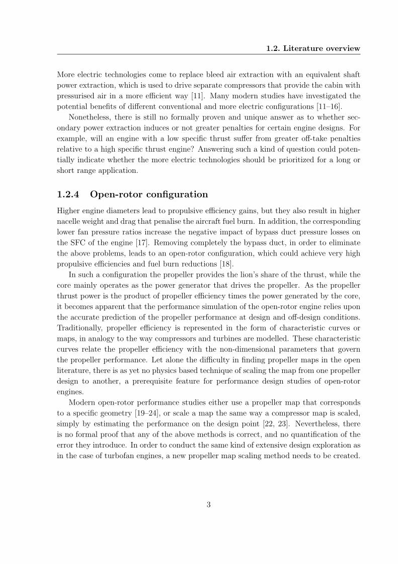
1.2.4 Open-rotor configuration

Higher engine diameters lead to propulsive efficiency gains, but they also result in higher

nacelle weight and drag that penalise the aircraft fuel burn. In addition, the corresponding

lower fan pressure ratios increase the negative impact of bypass duct pressure losses on

the SFC of the engine [17]. Removing completely the bypass duct, in order to eliminate

the above problems, leads to an open-rotor configuration, which could achieve very high

propulsive efficiencies and fuel burn reductions [18].

In such a configuration the propeller provides the lion’s share of the thrust, while the

core mainly operates as the power generator that drives the propeller. As the propeller

thrust power is the product of propeller efficiency times the power generated by the core,

it becomes apparent that the performance simulation of the open-rotor engine relies upon

the accurate prediction of the propeller performance at design and off-design conditions.

Traditionally, propeller efficiency is represented in the form of characteristic curves or

maps, in analogy to the way compressors and turbines are modelled. These characteristic

curves relate the propeller efficiency with the non-dimensional parameters that govern

the propeller performance. Let alone the difficulty in finding propeller maps in the open

literature, there is as yet no physics based technique of scaling the map from one propeller

design to another, a prerequisite feature for performance design studies of open-rotor

engines.

Modern open-rotor performance studies either use a propeller map that corresponds

to a specific geometry [19–24], or scale a map the same way a compressor map is scaled,

simply by estimating the performance on the design point [22, 23]. Nevertheless, there

is no formal proof that any of the above methods is correct, and no quantification of the

error they introduce. In order to conduct the same kind of extensive design exploration as

in the case of turbofan engines, a new propeller map scaling method needs to be created.

3

1. Introduction

1.3 Project aim and objectives

The aim of this project is to perform an exploration of the advanced turbofan design

space in order to identify the technologies required for different aircraft applications,

and to develop a propeller modelling approach that will enable the same exercise to be

conducted for an open-rotor configuration.

The work can be split into the following individual objectives:

1. the creation of an engine preliminary optimisation framework, which is able to cal-

culate the uninstalled performance, dimensions, weight, and installed performance.

The framework will be used in order to explain how the requirements of a given

aircraft application lead to the selection of a thermodynamic cycle.

2. establishing the link between the engine thermodynamic cycle and the requirement

for a variable area fan nozzle or a fan drive gearbox. Within the developed engine

optimisation framework, this connection will be then used in order to find whether

these enabling technologies should be prioritised for one aircraft application relative

to another.

3. the derivation of algebraic expressions that calculate the fuel consumption penalty

due to bleed and power extraction and the study of the thermodynamic cycle pa-

rameters effect. This entails answering the question whether future engines will

face higher penalties and intensify thereby the demand for more efficient secondary

power systems.

4. the creation of a propeller modelling method able to accurately model the perfor-

mance of prop-fan geometries. This capability will enable the generation and study

of full propeller maps for a given geometry.

5. the study of how the propeller map is affected when its design point changes, and the

creation of a generic propeller representation. This will allow the same map to be

used within extensive design parametric analyses, putting this way the foundations

for future open-rotor design exploration studies.

1.4 Thesis structure

The thesis starts by tackling objectives 1 and 2 within chapter 2. This chapter begins with

a brief account of engine efficiency and losses with the aim of identifying the parameters

driving them. Already existing studies concerning the need for a variable area nozzle or a

fan drive gearbox are reviewed. The method section presents the individual modules of the

preliminary optimisation framework and sets up the design exercise. The results section

4

1.4. Thesis structure

starts with the uninstalled performance results, continues with the relation between the

cycle parameters and the enabling technologies and concludes by the integration of all the

above in an installed performance analysis.

Chapter 3 deals with the secondary power off-takes study of objective 3. The analysis

starts by deriving formulas that calculate the effect of extracting bleed or power off-takes

on the core, transmission and propulsive efficiency of the engine. The equations are

subsequently validated by comparing their results against calculations conducted with

an engine simulation model. The chapter ends with a discussion on the thermodynamic

parameters that drive the efficiency penalties and the evolution of the penalties for future

engine designs.

Chapter 4 presents the development of a propeller modelling method in order to ac-

complish the objective 4. The literature survey covers the fundamentals of propeller

performance and reviews the available modelling methods. The development of the se-

lected approach is then described in detail. The chapter ends with the validation of the

method against experimental data and another higher fidelity method.

Chapter 5 starts by reviewing existing propeller map scaling approaches and by iden-

tifying their shortcomings. The propeller modelling method developed in chapter 4 is

then used in order to generate a full propeller map and use it to study the variations of

efficiency with the map parameters. A propeller optimisation framework is then set up

in order to calculate the optimal blade geometry for different design point specifications.

A full propeller map is then generated for each of the optimal geometries. The maps are

analysed and compared in order to devise a map scaling technique and accomplish this

way the objective 5.

The final chapter 6 summarises the most important findings of each technical part of

this work, identifies the novelty and the contribution to knowledge and ends with some

potential future work directions.

5

1. Introduction

6

Chapter 2

Advanced turbofan design space

exploration

2.1 Introduction

The work described in this chapter aims to demonstrate how a given aircraft applica-

tion leads to the selection of an optimum thermodynamic cycle, and to identify which

enabling technologies are required in order to implement it. The enabling technologies

under investigation include the installation of a fan drive gearbox and the use of a variable

area fan nozzle. It goes without saying that the presented topics have been extensively

treated within the design offices of the engine manufacturers, whose wealth of knowledge

on the topic is unrivalled. Nonetheless, their design choices are often driven by non-

thermodynamic factors and by underlying assumptions which are not always visible to

the academic reader. The presented analysis treats the subject from a clean sheet ther-

modynamic design perspective, in order to cast light to some of the current and future

design trends of the advanced turbofan engine.

The chapter starts by laying the foundations of engine losses and their dependencies to

the thermodynamic cycle parameters. Although seeming trivial, this topic is often a source

of misconceptions and is vital for the analysis to follow. The next step involves reviewing

the studies available on the literature showing the current trends of turbofan design, the

limits being reached and the required new technologies. The method description starts

by the presentation of the thermodynamic design framework used for the generation of

results. This framework combines an optimisation method with tools that calculate the

engine uninstalled performance, dimensions, weight, drag and installed performance. The

method description ends with the formulation of the optimisation design problem, which

also details the assumptions made for the case studies to follow. The case studies start

from the optimisation of the uninstalled engine performance, in order to identify the

7

2. Advanced turbofan design space exploration

effects of the main thermodynamic variables. The generated thermodynamic cycle data

are then fed into the engine design and weight tool, which calculates the dimensions of

the engine, the number of stages for each component and the engine weight. At this stage

the analysis establishes the relation between the thermodynamic cycle parameters and

the need for a variable area fan nozzle and a fan drive gearbox. The final stage of the

analysis involves the calculation of the installed performance for a short and a long range

aircraft mission. This calculation enables the positioning of the optimum engine designs

on the created design space maps, in order to demonstrate whether the industry trends

lead or not to the introduction of the aforementioned enabling technologies.

2.2 Engine Efficiency Fundamentals

The main power conversions that take place within a gas turbine aero-engine are depicted

in the schematic representation shown in Fig. 2.1. Although the schematic shows a

turbofan arrangement, the principles described apply also to turbojet and turboprop

engines.

Core

Fuel Power Power deliveredto the nozzles

Thrust

ThrustPower

Fan

Core Power

LPT

Bleed Air

Secondary Shaft Power

Figure 2.1: Schematic representation of a turbofan engine. The main power conversions

are also shown. The term core power describes the mainstream product of the core, while

the secondary power extraction consists of bleed air and shaft power.

Power enters the core of the engine in the form of fuel, which is burned inside the

combustor. The core translates the fuel power into hot gas thermal power at the core

exit (denoted as core power in Fig. 2.1), which is the mainstream product of the core. A

lower amount of power is extracted from the core as bleed air and secondary shaft power,

which comprise the total secondary power off-takes of the engine. At this point the core

efficiency can be defined as the ratio of mainstream core power over the power provided by

the fuel. The core efficiency, which corresponds to the thermal efficiency of a turboshaft

engine, depends on the engine overall pressure ratio and turbine entry temperature, and

on the isentropic efficiencies and pressure losses of the core components. It is common

8

2.2. Engine Efficiency Fundamentals

knowledge that for an ideal engine, the core efficiency always increases for an increasing

overall pressure ratio (OPR), while an optimum OPR exists if the component isentropic

efficiencies are lower than 100%. A different lower optimum value of OPR exists for the

maximisation of the core specific power. These optimum OPR values depend on the

turbine entry temperature (TET) and on the efficiency and pressure losses of the core

components.

On the other hand, the effect of TET is a source of many misconceptions. It is a

commonly held belief that the TET has no effect on the efficiency of an ideal engine,

while it has a positive effect for a non-ideal engine. At the same time, an increase in

TET always increases the specific power of the core and hence decreases its mass flow and

size for a given power requirement. According to Birch [2], under constant technology

level, after a certain value of TET, the resulting smaller core size and the increasing cool-

ing requirement completely counteract the efficiency amelioration. Nonetheless, the pure

thermodynamic effect of TET is considered always positive in terms of core efficiency.

This widespread statement regarding the effect on efficiency has been proven wrong sub-

sequently by Wilcock [25], Guha [26] and Kurzke [27]. The existence of this common

misconception originates from the simplifications made mainly for teaching purposes, in-

cluding constant heat capacities CP or the non-taking into account of the fuel mass flow.

Without these simplifications, the calculations result in the clear existence of an optimum

TET, which maximises the core efficiency and that is present even without the losses

induced by cooling bleeds or by smaller core components. The most sound explanation

has been given by Kurzke [27], who attributed the existence of the optimum TET in the

non-linear relation between the fuel injected in the combustor and the increase in temper-

ature. As the temperature increases, one has to introduce disproportionally higher fuel,

which finally leads to the deterioration of the engine core efficiency. Most surprisingly,

in the extreme case where the components are ideal, the TET is found to have always

a negative impact on core engine efficiency, a trend completely opposed to the common

knowledge. Nonetheless, it must be underlined that high TETs will always be used as a

way to decrease the core size and reduce its weight.

Kurzke’s finding has been confirmed by the author and the problem has been identified

in the combustor balance. The correct combustor balance as reported by Guha [26] is given

by Eq. 2.1, where the subscript g corresponds to ”gas” (air plus combustion products)

and the subscript a corresponds to ”air”. This non-linear relation between the enthalpy

at the combustor exit and the fuel air ratio is the reason for the existence of the TET

optimum. If the term (1 + far) is neglected, the result changes dramatically and no

TET optimum exists any more. Surprisingly, this term was neglected in the in-house

performance code (Turbomatch), and this was also the case with the excellent textbook

of Walsh and Fletcher [28]. Turbomatch has been corrected in order to capture correctly

this very important effect.

9

2. Advanced turbofan design space exploration

far · FCV = (1 + far) · hg04 − ha03 (2.1)

0 10 20 30 40 500.7

0.75

0.8

0.85

0.9

0.95

1

Bypass ratio

tr

f lpt = 0.86

f lpt = 0.79

f lpt = 0.72

Figure 2.2: Variation of transmission efficiency with bypass ratio, fan and turbine effi-

ciency.

Part of the hot gas power generated by the core is transmitted to the bypass propulsive

nozzle through the low-pressure turbine, fan, and bypass duct, whereas the remaining

power is transferred to the core nozzle. This power transfer is described by the so-called

transmission efficiency, which is defined as the ratio of power delivered to the propulsive

nozzles over the power generated by the core. The transmission efficiency is a function

of the engine bypass ratio, the low-pressure turbine and fan isentropic efficiencies, the

bypass and core duct pressure losses, while Guha [29] found that it also depends lightly

on the specific thrust of the engine. For the calculation of the transmission efficiency

many similar analytical expressions can be found in the literature [30–32]. Equation 2.2

is the one given in [32] and used for the analysis.

ηtr =1 +BPR

1 +BPR/(ηfηlpt)(2.2)

Figure 2.2 shows the variation of transmission efficiency with bypass ratio for different

sets of fan and low-pressure turbine isentropic efficiencies. The efficiency reduces as the

bypass ratio increases due to the higher amount of energy that is transmitted via the

higher losses path of the fan, low-pressure turbine, and bypass duct. At the one extreme,

in the case of a turbojet engine with BPR = 0, the transmission efficiency is equal to

10

2.2. Engine Efficiency Fundamentals

0 50 100 150 200 250 300

0.65

0.7

0.75

0.8

0.85

0.9

0.95

1

Specific Thrust [m/s]

pr

Figure 2.3: Variation of propulsive efficiency with specific thrust.

one. At the other extreme, when BPR →∞, all the energy is transferred to the bypass

stream and therefore ηtr → ηfηlpt.

Finally, as shown in Fig. 2.1, the power that reaches the propulsive nozzles is converted

into thrust power by the expansion of the air and hot gases into the atmosphere. This last

power conversion is described by the propulsive efficiency of the engine, which is defined as

the ratio of the thrust power produced over the power delivered to the propulsive nozzles.

ηpr =1

1 + ST/(2V0)(2.3)

The propulsive efficiency of a turbojet is given by Eq. 2.3, the derivation of which can

be found in many textbooks [33]. A graphical representation of Eq. 2.3 is shown in Fig.

2.3, where one can readily observe that as ST → 0, ηpr → 1. Equation 2.3 establishes the

unique dependence of propulsive efficiency on the engine specific thrust. This is a rather

intuitive result, if one considers that: 1) the propulsive efficiency represents the losses of

kinetic energy ejected in the atmosphere without producing thrust, 2) the specific thrust

is essentially equal to the increase in jet velocity as shown later by Eq. 2.6 and Eq. 2.7.

A similar expression can be derived for the case of separate flow turbofans, if one

assumes an optimum ratio of cold to hot jet velocities as shown by Eq. 2.4. Guha [34] has

proven that - for zero bypass duct pressure losses - the optimum ratio Vc/Vh equals the

product of the fan and low pressure turbine isentropic efficiencies. Equations 2.5-2.7 are

taken from the same reference [34] and define the kinetic energy in the nozzles, the mean

jet velocity and the specific thrust. Equation 2.5 makes the assumption of full expansion

at the nozzle exit, i.e. the static pressure is equal to the ambient and no pressure thrust

11

2. Advanced turbofan design space exploration

component exists. Combining Eqs. 2.4-2.7 leads to Eq. 2.8, which is the expression of

propulsive efficiency for a separate flow turbofan engine that has an optimum velocity

ratio. This assumptions seems to be a valid one according to the optimisation results

reported by Jackson [17] and Kyritsis [9]. It becomes apparent that in the case of a

turbofan engine, the propulsive efficiency is also affected by BPR and the low pressure

component efficiencies. However, their impact is much lesser relative to the impact of ST,

which remains the driving parameter. It is also observed that when ηfηlpt → 1, the BPR

drops from the equation and the expression reduces to Eq. 2.3. The performance results

by Bruni [35] also confirm the dominance of the ST factor, relative to the BPR term. In

general, the Eq. 2.3 could be used even for the case of a turbofan engine, within an error

of 0-5%.

This discussion comes to clarify another common misconception regarding the relation

between propulsive efficiency and BPR, also discussed by Refs. [2, 7, 29]. It is the ST

and not the BPR, which drives the propulsive efficiency. The two are interrelated only if

the core characteristics remain constant. For example, the BPR could be increased inde-

pendently from ST if the TET was increased, leaving the propulsive efficiency completely

unaffected. (VcVh

)op

= ηfηlpt (2.4)

Pnozzles = 1/2 ·Wh

(V 2h − V 2

0

)+ 1/2 ·BPR ·Wh

(V 2c − V 2

0

)(2.5)

Vm =1

1 +BPR

[BPR +

1

ηfηlpt

]Vc (2.6)

ST =T

Wh +Wc

= Vm − V0 (2.7)

ηpr =ST · V0

1/2 · (ST + V0)2 ·

(

1

(ηfηlpt)2 +BPR

)(1 +BPR)(

1

(ηfηlpt)+BPR

)2

︸ ︷︷ ︸

BPR term

−1/2 · V 20

(2.8)

Having defined the efficiencies of the aforementioned power transformations, the total

engine efficiency can now be expressed as the product of their individual efficiencies:

η0 = ηcoηtrηpr =PcorePfuel

PnozzlesPcore

PthrustPnozzles

=PthrustPfuel

(2.9)

12

2.3. Low pressure system enabling technologies

2.3 Low pressure system enabling technologies

After having explained the parameters driving engine efficiency, it becomes now clear why

engine design has followed a path of increasing TET, OPR and decreasing specific thrust.

Modern engines have take-off TETs in the order of 2000 K, maximum OPR which exceeds

50 and bypass ratios higher than 10 [29, 36]. Specific thrust values are more difficult to

quote as they are not usually reported by the engine manufacturers.

According to Refs. [27, 36, 37], no further core efficiency benefits are expected from

the increase of TET further than 2000 K. A further increase of around 3.5% is expected

for the core efficiency, mainly through the increase of OPR [6, 27]. The authors of Refs.

[2, 4, 17, 36] support that significant benefits can only arise from propulsive efficiency

gains, if the specific thrust is further reduced. According to Jackson [17] and Birch [2] this

could deliver an efficiency benefit close to 10% but only if the installation losses are kept

under control. On the other hand, Young [38] claims that in the case of medium to long

range aircraft, the specific thrust is not expected to reduce much further than the current

levels. Each of the above studies has been done under a different set of assumptions

and conducted at different times. Therefore it would be interesting to test the above

statements under a common set of assumptions for short and long range missions, with

current and future levels of technology.

Two low pressure system technologies are widely accepted as enablers of low specific

thrust designs. The first is the variable area fan nozzle (VFN), which is required in order

to control the fan surge at take-off conditions, from which suffer low fan pressure ratio

(FPR) engines. According to the analysis of Guha [34] low FPRs directly result from

a choice of a low specific thrust. Many different studies converge to the low limit FPR

value of 1.45, under which a VFN would be required [3–8]. Jackson [17] also calculated the

required percentage of fan nozzle area increase for a wide range of FPR values. Kyritsis

[9] investigated how a VFN can be further used in order to optimise the off-design engine

operation, or in order to enable a smaller and hotter core design. He studied the impact

on a specific engine design and found that none of the two options results in interesting

fuel benefits. Nonetheless, it would be interesting to expand this study on the whole of

the engine design space and test whether there is a design region when this variable cycle

technique brings significant fuel savings.

Contrary to the case of variable fan nozzles, there is no unique converged answer for

the introduction of a fan drive gearbox. Some authors relate the introduction of gearbox

to a bypass ratio greater than 10 [29, 36], while others for BPRs higher than 17 [30].

Zimbrick supported that a gearbox would be required in order to keep the number of low

pressure turbine stages below 6 [8]. References [4, 6, 37] introduce the gearbox for engines

which have an FPR lower than 1.4, while references [3, 7, 39] relate it to the specific

thrust of the engine, claiming a lowest ST value of 100 m/s for an ungeared configuration.

13

2. Advanced turbofan design space exploration

The assumptions underlying the aforementioned claims are not given, but two main

lines of thought recur in the literature. The first dictates that the gearbox should be

introduced to avoid an exceedingly high number of LPT stages, which could possibly

increase the weight, cost and length of the engine. The second perspective focuses on

the fact that a core must be flexible enough in order to accommodate a whole family

of engines [40]. Jacquet highlights the importance of the LP shaft diameter which must

pass through the core, and constitutes the parameter driving the growth capability of the

engine [41]. For constant fan power, the torque increases as the rotational speed decreases.

A higher torque sizes a higher diameter LP shaft, which becomes increasingly difficult to

fit through the HP shaft. Lower rotational speeds result from the constant fan tip speed

assumption, which keeps the aerodynamic losses under control, when the diameter of the

fan increases. Under a constant core assumption, the diameter of the fan can increase if

a growth version of the engine is sought and that is how the engine growth capability is

related to the flexibility of the core, and the LP shaft diameter. According to Borradaile

[3] a core which has been designed for an engine of given specific thrust, immediately

poses a torque limit on the LP shaft, which could only be overcome by introducing a

gearbox or an aft-fan configuration.

The analysis by Kurzke is the only one existing in the open literature, which clearly

describes its ground rules [36]. This study compares the characteristics of a conventional

and a geared configuration, as the bypass ratio increases under a constant core assumption.

Both the problem of increasing LPT stages number and LP shaft torque are demonstrated

and the author concludes that at a BPR of 10 the two configurations are equal, with

the geared architecture becoming more appealing as the BPR increases further. Kurzke

clearly connects the use of a gearbox with BPR or specific thrust. It is reminded that

under constant core conditions the two parameters are directly linked. Thus, it is unclear

which of the two parameters is the one driving the phenomena, or whether the core

characteristics have any influence. Furthermore, the aim of the paper is to compare the

two configurations under the same thermodynamic cycle parameters. However, a geared

configuration is expected to have a lower specific thrust optimum [5] and therefore a

further propulsive efficiency benefit to unlock.

The work presented in this chapter aims to extend Kurzke’s study and to fill the

aforementioned gaps. Nevertheless, it has been chosen not to follow a constant core

assumption, as this would require the selection of a core size according to some given

engine family strategy. Such a selection could only be performed correctly within the

preliminary design office of an engine manufacturer and is outside the scope of this work.

Thus, the current analysis will mainly focus on the number of LPT stages aspect and its

connection to the thermodynamic cycle characteristics.

14

2.4. Numerical methods and models used

2.4 Numerical methods and models used

2.4.1 Engine model - TURBOMATCH

The performance simulation is conducted using the Turbomatch code, developed in Cran-

field University. This code is based on the equations of mass continuity and energy bal-

ance, combined with characteristic curves or ”maps” that describe the performance of

the individual components. The set of the above non-linear equations is solved using an

iterative Newton-Raphson solver. More details on Turbomatch can be sought in [42].

The code has been upgraded by the author on the following aspects:

Convergence robustness

• The component maps have been ”smoothed” in order to increase the accuracy

of the interpolations.

• The non-linear Newton-Raphson solver has been upgraded by adding the back-

tracking capability, which improves the global convergence as described by

Press et al [43]. This change was essential in order to avoid the numerous

convergence problems encountered with the initial version of the code, which

made the integration with an optimiser very difficult.

• In extreme cases, where one of the nozzles has barely enough pressure ratio

to eject the fluid to the atmosphere, convergence problems can still occur.

To tackle these problems the author added the capability of automatically

adjusting the off-design steps requested by the user in order for them to be

small enough for the solver to converge.

• The ability of convergence even outside the component maps was introduced.

Before this change, if the solution tried to move outside the limits of a compo-

nent map, the code would immediately intervene in the solution proposed by

the solver and move the solution inside the allowed space. This could easily

lead to singular Jacobian problems for solutions that lied close to the limits of

the maps. Furthermore, this new capability allows the illustration of the fan

surge problems from which suffer the low FPR fans.

• A solver guess has been added for the intake mass flow. Previously, the intake

mass flow was only known when the first compressor of the flowpath was cal-

culated. This meant that the initial mass flow at the intake had to be taken

from the previous numerical step, in order to calculate the momentum drag.

This numerical lag between the intake mass flow and the rest of the variables

was found to lead to convergence problems.

15

2. Advanced turbofan design space exploration

• The turbine mass flow guess has been replaced by the turbine non-dimensional

enthalpy drop, which corresponds to its pressure ratio. This modification al-

lowed the solutions to lie in the choked region of the turbine map where the

mass flow is constant.

The above convergence related modifications have an important impact on the robust-

ness of the code. Before the modifications, the lowest achievable idle thrust was about 20%

of the maximum take-off thrust, in the case of a separate flow turbofan engine. Moreover,

in order to achieve this idle thrust, the user had to specify many small off-design steps

from maximum take-off until idle. Getting closer to idle, these steps could be even less

than 10 K of TET. After the aforementioned stability improvements, the lowest possible

thrust can be as low as 7%, achievable with only one step from maximum take-off.

Features enrichment and improvements

• The capability of using the engine thrust as a power setting handle has been

added. This allows the automatic adaptation of the engine TETs in order to

satisfy the given thrust requirements. Previously, the user could only define a

TET and calculate the thrust as a result. This meant that the TET had to be

iterated by the user until the desired thrust value was achieved. In order to

automate the process and enable the execution of thousands of optimisation

cases, this task has been taken on by the code solver, which automatically

calculates the required TET.

• A propeller component has been added in order to incorporate the findings on

propeller modelling as described in chapters 4 and 5.

• The capability of defining the compressor polytropic efficiency has been added.

This allowed the fair comparison between compressors of different pressure

ratios as described by Saravanamuttoo et al [44]. The same process has not

been introduced for turbines as their pressure ratio shows much lower variation.

Furthermore, in the turbine case an additional iteration would be required,

which would unnecessarily increase the complexity as described by Kyritsis [9].

• The combustor balance has been updated in order to take into account the

injected fuel flow as described in section 2.2. This change resulted in optimum

TETs lower by 200K, a result with significant impact on engine design and

lifing considerations.

• The capability of programming one engine variable as a function of another

was introduced. This improvement allowed the scheduling of bleed valves or

variable stator vanes as a function of the power setting of the engine.

16

2.4. Numerical methods and models used

2.4.2 Engine preliminary design and weight estimation tool

The preliminary design tool is fed with the engine thermodynamic parameters generated

by Turbomatch, conducts a preliminary sizing of the main components and estimates the

weight of the engine. The tool has been created in Cranfield University by Lolis and

a detailed description and validation can be found in his PhD thesis [45]. Apart from

the engine thermodynamic data, the design code requires the definition of certain de-

sign assumptions for each component. These design assumptions include the definition

of component input and output Mach numbers, hut to tip ratios, aerodynamic loadings

and geometrical choices, like constant hub, tip or meanline. The whole engine meridional

design is calculated by the code including the component number of stages, diameters,

lengths, rotational speeds and the variation of aerodynamic and thermodynamic param-

eters within the component. The code has been validated by Lolis, achieving almost

identical designs when compared to current engines and providing consistent weight pre-

dictions. The interaction between Turbomatch and the design code has been completely

automated by Lolis, thereby giving the capability of running efficiently a large number of

engine design studies.

2.4.3 Installed performance calculation

Having calculated the engine weight for each one of the engine thermodynamic cycles, two

more elements are required before the calculation of the installed performance. The engine

nacelle weight and drag. The nacelle weight is calculated using Eq. 2.10, as proposed by

Jackson [17].

mnac = κnac · (2 · Lc · dc + Lb · da + 2 · La · da) (2.10)

The coefficient κnac represents the nacelle weight per square meter of nacelle surface

and Jackson calculated it equal to 24.88[kg/m2] for an engine similar to the RR Trent

892. The explanation of the individual variables is given by Fig. 2.4. As shown in Eq.

2.10, Jackson multiplied by 2 every surface which is exposed to the atmosphere. In order

to simplify the calculation and without losing much accuracy, this has not been taken

into account for the case of the afterbody (described by the length La). Thus the two last

terms collapse into one which equals to (Lb + La) · da. This term can then be calculated

if the length of the fan module is subtracted from the total engine length. The diameters

dc and da are taken equal to the fan and booster inlet tip diameters respectively.

Engine drag is the last required element and it is calculated using the method suggested

by Walsh and Fletcher [28], also used by Jackson [17]. According to this approach, the

nacelle drag can be calculated as the sum of the cowl and afterbody drag by Eq. 2.11-

2.13. The factor κi represents the interference drag and according to Jackson it is taken

17

2. Advanced turbofan design space exploration

Figure 2.4: Engine schematic showing the definition of nacelle dimensions

equal to 1.2. According to Walsh and Fletcher [28] the drag coefficient CD takes a value

between 0.002-0.003. The value 0.003 is used by Jackson, while the low limit of 0.002 is

chosen for this study. It must be highlighted that the velocity used for the calculation

of the afterbody drag (Eq. 2.12) is not the free stream one, but the one ejected by the

bypass nozzle. Finally, the cowl length to diameter ratio depends on the type of cowl and

its technology. A long cowl would have values from 1.5 to 1.8, while an aggressive short

cowl could have values even below 1 [17].

Dc = κi ·1

2· ρ · V 2

0 · CD,c ·[π ·(L

D

)c

· d2c

](2.11)

Da = κi ·1

2· ρ · V 2

c · CD,a · (π · La · da) (2.12)

Dn = Dc +Da (2.13)

Knowing the uninstalled engine SFC, weight and drag, the installed performance can

now be calculated using the range factor Kr introduced by Walsh and Fletcher [28], Eq.

2.14. The engine fuel burn FB is calculated using Eq. 2.15. The range factor is effectively

an installed expression for the specific fuel consumption, expressed as total engine related

mass divided by the installed engine thrust. Contrary to the uninstalled SFC, this ex-

pression takes into account the engine weight and drag variation. The equation considers

that the required thrust at mid-cruise remains constant as the engine parameters vary and

thus represents more accurately the case of re-engining a fixed aircraft. This approach

would give somewhat conservative predictions if the aircraft was changing in relation to

the efficiency to the engine.

18

2.5. Engine design principles

Kr =Me + FB

TmCR −Dn

(2.14)

FB = TmCR · SFCmCR ·Range

V0

(2.15)

2.4.4 Optimisation method

The purpose of this section is not to describe in detail different optimisation algorithms

but to justify the selection of the optimisation method used within the created engine

optimisation framework. For further information the reader can refer to several good

textbooks on this topic [46, 47]. The nature of the engine design problem falls into

the category of non-linear constrained optimisation. The method selected is a Genetic

Algorithm developed in Cranfield by Rogero [48] and used later on also by Celis [49].

The reason for starting the optimisation with a genetic algorithm emerges from the fact

that the non-linear equations governing the design of the engine do not have a solution for

any given set of design variables [50]. For instance, increasing too much the fan pressure

ratio for a given set of (TET, OPR, BPR) can lead to a core nozzle pressure ratio which

is lower than one, and hence to a non-feasible solution. Furthermore, gradient methods

require that the function to be optimised is smooth enough for the determination of

the gradients [51]. As seen in section 2.4.1, the prediction of engine performance relies

a lot on the interpolation of characteristic curves and on iterative methods with given

tolerances. At this moment, the tolerance of Turbomatch is in the order of 5×10−4. This

tolerance is adequate for engine simulation, but it is quite large if Turbomatch has to be

used by another numerical method, such as an optimiser. Therefore, the discontinuities

present on the characteristic curves and the inadequate convergence tolerance are potential

sources of problems for gradient based methods. On the other hand, Genetic Algorithms

have been successfully used in previous engine simulation studies at Cranfield University

[48, 49, 52–54]. After experimenting with a gradient based approach included in Matlab

and the GA optimiser available in the department, the latter has been chosen mainly due

to its robustness and accurate results.

2.5 Engine design principles

During the preliminary design phase the engine thermodynamic cycle parameters are

chosen in order to comply with the requirements of the following three major mission

points [55, 56].

• hot-day take-off (TO) The requirements of the airframe manufacturer for a given

runway length and a minimum climb rate pose a thrust requirement for the engine

19

2. Advanced turbofan design space exploration

at this point. The highest engine temperatures and spool speeds are usually en-

countered at this point and that is why the mechanical design of the engine takes

place here.

• Top-of-climb (ToC) At this point the fan experiences its highest non-dimensional

mass flow and speed. Minimum time to cruise and air traffic control restrictions

impose a thrust requirement for this point too.

• Mid-cruise (mCR) For civil aircraft the figure of merit is normally the mission

block fuel. The greatest part of the fuel is burned at cruise and thus the SFC at a

typical mid-cruise point constitutes an important performance metric.

The thermodynamic design point can be located either at top-of-climb [49, 55, 57] or

at mid-cruise [51, 58]. In the first case the design points must be located in such a way on

the component maps that the optimum component efficiencies occur at mid-cruise [57].

In the second case a margin must be allowed for the increased aerodynamic speed of the

top-of-climb condition [58].

In order to fully define the thermodynamic design of a two-spool separate exhausts

turbofan, where the design point is located at mid-cruise, the following thermodynamic

parameters must be chosen [9]:

1. Bypass ratio at mCR

2. Fan pressure ratio at mCR

3. HP/LP pressure ratio split at mCR

4. Overall pressure ratio at mCR

5. Engine mass flow at mCR

6. Combustor outlet temperature at mCR

7. Combustor outlet temperature at ToC

8. Combustor outlet temperature at TO

The designed engine has to satisfy the following set of constraints, coming either from

airframe requirements or technological limitations:

1. a mid-cruise nominal net thrust TmCR

2. a hot-day take-off nominal net thrust TTO

3. a top-of-climb nominal net thrust of TToC

20

2.6. Engine thermodynamic design approach

4. a maximum fan diameter of df imposed by the airframer

5. a hot-day take-off maximum turbine entry temperature TETTO

6. a hot-day take-off maximum high-pressure compressor exit temperature of T3,TO

The fan diameter can be calculated at top-of-climb if typical values of the hub-tip ratio

and inlet Mach number are assumed. The thrust at the take-off and top-of-climb points

can be replaced by the ratios of thrust relative to the mid-cruise point, which do not

depend on engine size but only on its thermodynamic parameters. Although traditionally

only the maximum take-off TET is taken into account, according to Karanja [40] an eye

must be kept at the levels of TET at climb and cruise in order to control the creep life of

the engine. The compressor delivery temperature limit is imposed by the requirement for

uncooled compressor blades, with an approximate limit of 990 [K] for nickel alloy blades

[29]. Finally, the figure of merit can either be the engine specific fuel consumption, if

only the uninstalled performance is optimised, or the mission block fuel in the case where

the optimum installed performance is sought. In the context of this work the installed

performance optimisation is optimised using the aforementioned range factor Kr presented

in section 2.4.3.

2.6 Engine thermodynamic design approach

The selection of the thermodynamic parameters that define the engine cycle is normally

conducted either by extensive parametric studies or numerical optimisation. Parametric

studies give a physical insight on the phenomena that govern the engine performance,

but they are not suitable for cases with more than 2-3 design variables and numerous

design constraints. This is true especially when only one parameter is varied while all

the others are constant at a non-optimum value [29]. Numerical optimisation can then

be employed to find an optimum solution that satisfies all the design constraints [59].

Nonetheless, numerical optimisation results must always be critically filtered, otherwise

they are just numbers coming out of a black box. Both the aforementioned approaches

have their merits, and within the context of this thesis a combination of the two will be

implemented.

To begin with, it must be noted that contrary to formal definitions, the turbine entry

temperature (TET) signifies the combustor outlet temperature. That is the temperature

before the mixing of the nozzle guide vanes cooling flow. The method used here for the

thermodynamic cycle design is essentially similar to the approaches of Jackson [17] and

Guha [29]. A typical mid-cruise point of given thrust is used as the engine design point.

This choice is based on the fact that the engine off-design performance is calculated using

component characteristic curves, interpolation and a numerical solver process, which at

21

2. Advanced turbofan design space exploration

the moment is not accurate enough. On the other hand, the design point calculation

uses no iterative process and thus achieves by default a very high accuracy. Thus this

selection avoids the interaction of the engine off-design iterative process with the optimiser

and enables a more robust and accurate optimisation. For a parametric variation of the

design point turbine entry temperature, overall pressure ratio and bypass ratio, the fan

pressure ratio is optimised for minimum design point SFC. The optimisation of the fan

pressure ratio leads to an optimal ratio of velocities between the bypass and core nozzle as

described by Guha [34]. This technique, also used by Jackson [17], intrinsically assumes

that the FPR does not have an important impact on the fan weight. By using this design

approach the main design variables have been essentially reduced to 3 (TET, OPR, BPR)

and a clear graphical representation of the design space is enabled.

Kyritsis proved that the engine performance does not depend on its actual size, as

long as there is no constant absolute demand for power or bleed off-takes [9]. Therefore,

it has been decided not to include any normal off-takes and thereby avoid the iteration of

inlet mass flow in order to match a given design point thrust. This technique simplified

significantly the optimisation task. The effect of off-takes will be separately treated in

chapter 3.

Having optimised the design point FPR for the given values of TET, OPR and BPR,

the off-design conditions of ToC and TO can be now calculated using the thrust ratios

(independent of design point thrust). These thrust ratios are automatically matched by

Turbomatch using its internal iteration process that calculates the required off-design

TETs. At this point the engine performance is known at all the three major design points

for the given set of TET, OPR and BPR. An extensive variation of these three parameters

unfolds the design space, where the benefits in SFC can be juxtaposed with the different

engine design constraints, identifying this way the optimum feasible solution. The process

can be repeated for different thermodynamic assumptions, notably for different component

efficiencies. Nevertheless, the final optimal solution can not be identified yet, as at this

point only the uninstalled performance is known.

The next step involves the calculation of engine enabling technologies using the pro-

duced uninstalled thermodynamic results. Plotting the fan surge margin at take-off for

each engine design allows to identify the need for a variable fan nozzle. At this point, the

engine mass flow is scaled to provide the required design point thrust and the performance

results are passed on the preliminary design code in order to calculate the number of LPT

stages, the dimensions of the engine and its weight. The dimensions of the engine are

subsequently used in order to calculate the engine drag and finally the range factor Kr

for a specified aircraft mission. This installed performance calculation is then repeated

for long and short range missions. The data generation process is now completed and

the analysis of the design space can be conducted. Tracing the installed performance on

design space maps, enables the selection of an engine respecting the design constraints

22

2.7. Uninstalled performance study

and allows the quantification of the impact of the aforementioned technologies.

2.7 Uninstalled performance study

2.7.1 Model configuration and assumptions

The baseline engine model employs a two-spool separate flow turbofan configuration as

shown in Fig. 2.5. The basic thermodynamic design assumptions are shown in table

2.1. The polytropic efficiency is used for the compressors in order to isolate the effect

of technology level from the effect of pressure ratio variations. On the other hand, the

same approach is not followed for the turbines, because this capability is not supported

by Turbomatch and its implementation would require additional iterations within the

turbine module. The same approach was followed by Kyritsis [9]. This gives a somewhat

pessimistic view of the turbine efficiency, which however does not give unrealistic results,

because turbines have significantly lower pressure ratios relative to compressors. The

nozzles are assumed to have an ideal velocity coefficient CV as the characteristic curve

available in Turbomatch gave unexpectedly low values. Jackson [17] also assumed an

almost ideal value of 0.999.

Figure 2.5: Engine configuration schematic showing the definition of OPR, T3 and TET.

The bypass and core nozzles are designated by BPN and CN respectively.

The fan module is modelled as a simple compressor component, as Turbomatch does

not support a separated hub/tip modelling. In order to conserve the OPR as the fan

pressure ratio varies during the optimisation, the model automatically adjusts the pressure

ratio of the booster (LPC) and the HPC, by conserving their relative ratio of PR at the

value shown in table 2.1. The additional optimisation of the pressure ratio split between

23

2. Advanced turbofan design space exploration

the two compressors would require studying the impact of compressor pressure ratio on

its polytropic efficiency, while also taking into account the variation of HPT stages. For

example, the HPC pressure ratio could be limited in order to have only one HPT stage,

limiting this way the number of expensive HPT parts. As the above considerations are

outside the scope of this thesis, the simplifying assumption of constant pressure ratio split

is made.

The relative cooling mass flow Wcl/W25 is considered constant as the OPR and TET

vary. This essentially means that the cooling technology is adjusted in order to maintain a

constant metal temperature, or that the maximum allowable metal temperature changes.

A varying cooling mass flow would move the optimum results towards lower OPR and

TET but its calculation falls outside the scope of this work.

Finally, table 2.1 shows the specifications of the three major design points. The two

mid-cruise thrusts correspond to typical short range and long range aircraft and they will

be used for the sizing calculations of the installed performance study, later on. The thrust

ratios come from the airframe requirements and constitute typical short and long range

values.

Table 2.1: Engine thermodynamic specifications

Parameter Value Parameter Value

mid-cruise 35kft/0.8M/ISA Wcl/W3 10 [%]

top-of-climb 35kft/0.8M/ISA+10 ηp,c 0.85/0.90/0.95

take-off SLS/ISA+15 ηis,t 0.85/0.90/0.95

Short range TmCR 20 [kN] PRHPC/PRLPC 11

Long range TmCR 65 [kN] CV 1.0

TToC/TmCR 1.325 Bypass duct ∆p/p 1.5 [%]

TTO/TmCR 6.05 Burner ∆p/p 4.0 [%]

2.7.2 Uninstalled performance results

Figure 2.6 shows the variation of the optimum FPR with design point (mCR) TET and

BPR, while also illustrating the impact of the aforementioned parameters on the non-

installed cruise SFC. The main observations stemming from this figure are the following:

• For a constant BPR the optimum FPR increases as the TET increases.

The optimum FPR corresponds to the FPR which leads to an optimum ratio of jet

velocities Vc/Vh = ηfηlpt. Under constant BPR conditions the mass flows of the two

24

2.7. Uninstalled performance study

streams are fixed. If the FPR also remained constant, the total fan power would stay

the same and the same would apply for the LP turbine. Thus the turbine enthalpy

drop would also be fixed. At the same time, the increase in TET would increase

the specific power of the core, and thus for the same core mass flow more enthalpy

would be available at core exit. At constant turbine power this increased enthalpy

would translate to an increased core nozzle velocity. However, the bypass stream

jet velocity would be the same as it is fixed by the FPR, and thus the jet velocity

ratio would decrease away from its optimum value. Its a natural consequence that

the FPR has to increase in order to increase the cold jet velocity, decrease its hot

counterpart and bring back the velocity ratio at its optimum value.

1200 1400 1600 1800 2000

5

10

15

20

25

30

TET [K]

BPR

d = 90% & OPR = 30

1.2

1.3

1.45

1.6

1.85SF

C [g

/kN

/s]

13

14

15

16

17

18

19

20

Figure 2.6: Baseline uninstalled SFC design map, also showing the variation of optimum

FPR (white lines).

• For a constant TET the optimum FPR decreases as the BPR increases.

With a fixed TET the specific enthalpy at the core exit is constant (enthalpy for

unit mass). For a fixed FPR, the LPT enthalpy drop depends only on the ratio of

LPT and fan mass flows, i.e. on the bypass ratio. For higher BPR the fan mass

flow increases while the LPT mass flow is constant and thus the LPT turbine has

to work harder and its enthalpy drop increases. This drops the velocity of the core

nozzle and thus for fixed cold velocity (fixed FPR) unbalances the optimality of the

velocity ratio. Therefore, the FPR has to be reduced in order to increase the velocity

ratio to its optimal value. In reality, the LPT mass flow would not remain constant

and it would adjust up or down in order to give a fixed thrust value. The direction

of the LPT mass flow change would depend on whether or not the optimum BPR

25

2. Advanced turbofan design space exploration

value has been exceeded or not. If the increase in BPR improves the efficiency then

for the same thrust a smaller core would be needed and thus the LPT mass flow

would decrease, together with a decrease in the fan mass flow, in order to keep the

desired BPR value.

• For a constant BPR there is an optimum TET which minimises SFC. The

existence of an optimum TET for a given BPR results from the trade-off between

propulsive and core efficiency (the transmission efficiency being fixed by the constant

BPR). For the given OPR and component efficiencies, the increase in the TET

leads to an initial improvement of the core efficiency, until approximately a TET

of about 1800 K. For higher component efficiencies or lower OPR this optimum

TET would move towards lower values. In the extreme case where ideal component

efficiencies were considered, the increase in TET would only have a negative impact

on the efficiency for the reasons discussed in section 2.2. Concerning the propulsive

efficiency, an increase of TET under constant BPR conditions leads to an increase

in FPR and jet velocities and thus to a decrease of propulsive efficiency. For higher

BPR the optimum TET, moves to the right due to the positive effect of reduced

FPR and jet velocities.

• For a constant TET there is an optimum BPR which minimises SFC. This

time the trade-off takes place between the propulsive and the transmission efficiency.

As the BPR increases the FPR and jet velocities decrease and the propulsive effi-

ciency improves. At the same time more energy travels through the bypass system

and thus the transmission efficiency decreases. The transmission efficiency being of

secondary importance, the optimum BPR presents quite high values. An increase

in TET leads to increased jet velocities and thus the optimum BPR is moved to

higher values.

The aforementioned analysis was conducted under constant OPR and component effi-

ciency conditions. The effect of altering these conditions is treated by Fig. 2.7a and 2.7b,

for which the following statements can be made:

• An increase in the OPR leads to decreased optimum FPR values. This

statement stems from the current design trends of civil aircraft engines, but it is

not necessarily correct according to the strict thermodynamic theory. In theory,

there is an value of OPR which maximises the specific work output of the core. If

the baseline value of OPR is lower than this value, the increase of OPR leads to

an increase in specific work, while the opposite applies if the baseline value lies on

the right of the value that maximises the specific work. Civil aircraft engines are

designed for maximum efficiency and thus the OPR is always close to the value

that maximises the efficiency and on the right of the maximum specific work point.

26

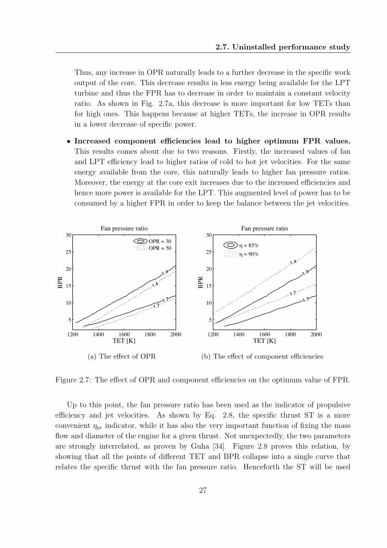
2.7. Uninstalled performance study

Thus, any increase in OPR naturally leads to a further decrease in the specific work

output of the core. This decrease results in less energy being available for the LPT

turbine and thus the FPR has to decrease in order to maintain a constant velocity

ratio. As shown in Fig. 2.7a, this decrease is more important for low TETs than

for high ones. This happens because at higher TETs, the increase in OPR results

in a lower decrease of specific power.

• Increased component efficiencies lead to higher optimum FPR values.

This results comes about due to two reasons. Firstly, the increased values of fan

and LPT efficiency lead to higher ratios of cold to hot jet velocities. For the same

energy available from the core, this naturally leads to higher fan pressure ratios.

Moreover, the energy at the core exit increases due to the increased efficiencies and

hence more power is available for the LPT. This augmented level of power has to be

consumed by a higher FPR in order to keep the balance between the jet velocities.

1200 1400 1600 1800 2000

5

10

15

20

25

30

TET [K]

BPR

Fan pressure ratio

1.4

1.7

1.4

1.7

OPR = 30OPR = 50

(a) The effect of OPR

1200 1400 1600 1800 2000

5

10

15

20

25

30

TET [K]

BPR

Fan pressure ratio

1.4

1.7

1.4

1.7

d = 85%d = 90%

(b) The effect of component efficiencies

Figure 2.7: The effect of OPR and component efficiencies on the optimum value of FPR.

Up to this point, the fan pressure ratio has been used as the indicator of propulsive

efficiency and jet velocities. As shown by Eq. 2.8, the specific thrust ST is a more

convenient ηpr indicator, while it has also the very important function of fixing the mass

flow and diameter of the engine for a given thrust. Not unexpectedly, the two parameters

are strongly interrelated, as proven by Guha [34]. Figure 2.8 proves this relation, by

showing that all the points of different TET and BPR collapse into a single curve that

relates the specific thrust with the fan pressure ratio. Henceforth the ST will be used

27

2. Advanced turbofan design space exploration

analogously to FPR, as done in Fig. 2.9a, which corresponds to the analysis of Fig. 2.6.

It must be underlined that throughout this chapter the term ST refers to the specific

thrust at the top-of-climb point, as it is this point that sizes the fan diameter. It can be

observed from Fig. 2.9a that there is an optimum value of ST which is around 75 m/s, a

value which according to Guha [60] is much lower than the currently applied levels of ST.

This difference is due to the effect of drag and weight, not captured by the uninstalled

SFC, as explained in section 2.4.3.

1 1.2 1.4 1.6 1.80

50

100

150

200

250

Fan pressure ratio

ST [m

/s]

Figure 2.8: The relation between specific thrust (ST) and FPR (η = 90% OPR = 30).

The plotted points represent results for the full range of TET and BPR.

Figure 2.9a shows another interesting aspect concerning the choice of TET. Following

a constant ST line (e.g. ST = 150m/s) the engine soon reaches a point where a further

increase in TET does not bring any benefits. Under constant ST conditions, the propul-

sive efficiency is fixed and the trade-off takes place between the core and transmission

efficiencies. As the TET increases the core efficiency increases before it reaches an op-

timum value at about 1800-1900K. Results proving this statement can be found in the

aforementioned works of Guha [26], Wilcock et al. [25] and Kurzke [27]. At the same

time, for higher TETs the BPR increases in order to conserve a fixed value of ST. This

increase in BPR brings about a degradation of the transmission efficiency. The ensemble

of the above effects leads to the existence of an optimum TET very close to the currently

used values. The phenomenon is accentuated if higher component efficiencies are used,

as shown in Fig. 2.9b. The higher component efficiencies significantly decrease the TET

value that optimises the core efficiency and hence from an efficiency point of view, in-

creased TETs are completely uneconomical. Nonetheless, high TETs can still be used

28

2.7. Uninstalled performance study

as a means to decrease the core size and weight. These results confirm the observations

made by Guha [29], and are completely opposed to the widely held belief that from an

efficiency point of view, high TETs are always beneficial.

1200 1400 1600 1800 2000

5

10

15

20

25

30

TET [K]

BPR

d = 90% & OPR = 30

50

75

100

150

200 SFC

[g/k

N/s]

13

14

15

16

17

18

19

20

(a) Baseline map

1200 1400 1600 1800 2000

5

10

15

20

25

30

TET [K]BP

R

d = 95% & OPR = 30

50

75

100

150

200 SFC

[g/k

N/s]

11

12

13

14

15

16

17

18

19

20

(b) The effect of component efficiencies

Figure 2.9: The uninstalled SFC design map, using the specific thrust as a design param-

eter.

2.7.2.1 The TET ratio between take-off and climb

This short section deals with the TET ratio between take-off and climb/cruise and its

variation throughout the design space. Jackson [7] stated that the lower the specific

thrust the higher the TET at ToC relative to the ones observed at TO. This observation

is confirmed by the results shown in Fig. 2.10, covering different TET, BPR, OPR and

component efficiencies. There is a clear relation between ST and the ratio of TET,

although there is some scatter of the points in the two extremities. This scatter is due to

the variation of the fan efficiency for the extreme values of ST. As shown by Fig. 2.11, at

very low ST the fan operating point at TO is above the surge line (see section 2.8.1), while

at very high ST it moves towards the right extreme where the efficiency start degrading

faster. Especially the points above the surge line are completely unrepresentative, as the

fan efficiency results from extreme extrapolations.

The clear relation between the specific thrust and the TET ratio can be explained

by the connection of ST to the jet velocities. A low ST leads to low jet velocities and

a higher amount of thrust produced by the mass flow component. The higher the mass

flow component of the thrust, the higher the sensitivity to the increases of Mach number

and altitude. The sensitivity to Mach stems from the stronger component of momentum

drag, which is proportional to the inlet mass flow of the engine. The sensitivity to the

29

2. Advanced turbofan design space exploration

increase of altitude comes from the decrease in the air density, which directly impacts the

mass flow and hence the thrust. Under constant TET between ToC and TO, and a fixed

thrust at ToC, a higher thrust lapse rate leads to a higher thrust at TO. However, the

thrust at TO is also fixed by aircraft requirements and thus the TET has to fall at TO

in order to keep the thrust constant. That is the reason why lower ST, leads to TETs at

climb which are closer to the ones at TO, or even higher. This conclusion shows another

important impact of ST on engine design, operation and finally cost. Low ST engines, will

experience much higher temperatures at climb and cruise (for a fixed maximum take-off

temperature) and thus a significantly higher amount of their life will be consumed due

to creep. At the same time, the cooling flow will probably have to be sized for the ToC

point, if the maximum TET moves there. Alternatively, the design might choose to lower

the temperatures at every operating point, or even to choose a higher ST, degrading this

way the propulsive efficiency. The final decision, would depend on all the aforementioned

aspects and is an answer that depends on the strategy and characteristics of the engine

manufacturer.

0 100 200 300 400 500 600

0.9

1

1.1

1.2

1.3

ST [m/s]

TET

@TO

/ TE

T @

MCL

d = 85% & OPR = 30d = 85% & OPR = 40d = 90% & OPR = 30

Figure 2.10: The relation between specific thrust (ST) and the ratio of TET between ToC

and TO. The plotted points represent results for the full range of TET and BPR.

2.7.2.2 Design space limits for the selection of OPR

The overall pressure ratio (OPR) is selected in a way that optimises the efficiency of the

core. The optimum OPR depends on the TET of the engine, according to the principle

that a higher TET leads to a higher optimal OPR. Increasing the OPR further would

degrade the core efficiency, unless a higher TET was employed. Figure 2.12 illustrates

30

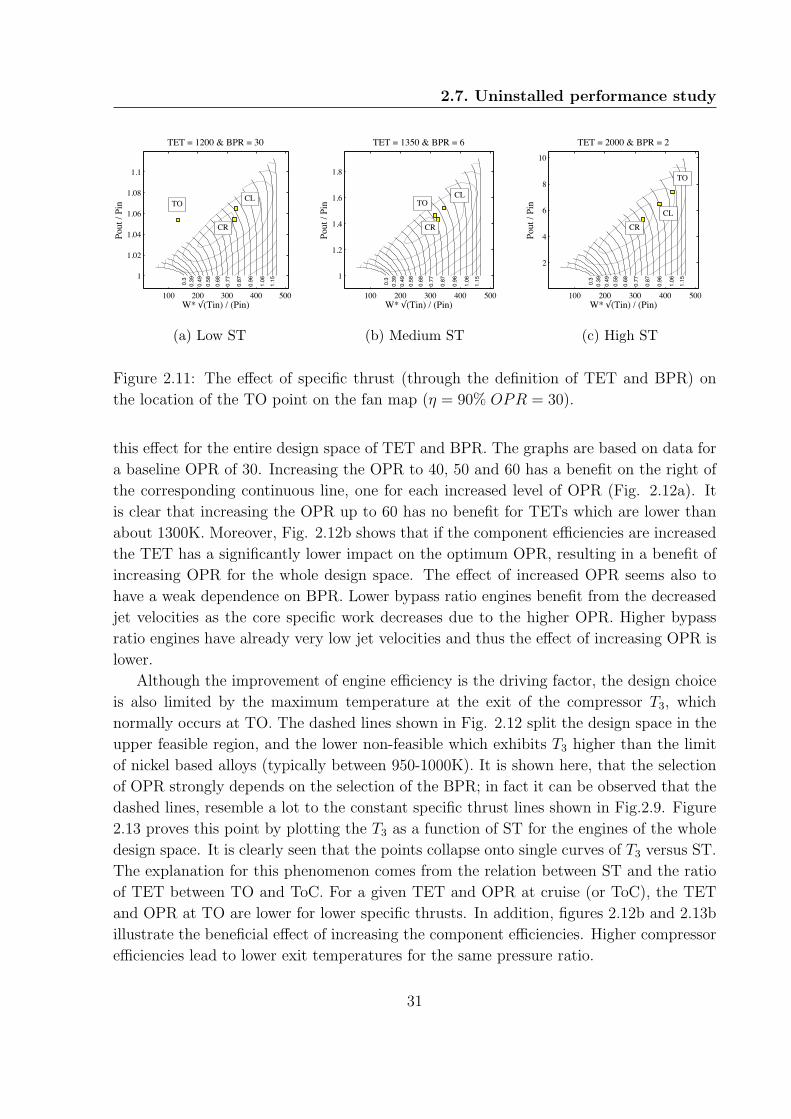
2.7. Uninstalled performance study

100 200 300 400 500

1

1.02

1.04

1.06

1.08

1.1

W* 3(Tin) / (Pin)

Pout

/ Pi

n

TET = 1200 & BPR = 30

0.3

0.39

0.49

0.58

0.68

0.77

0.87

0.96

1.06

1.15

CR

TO CL

(a) Low ST

100 200 300 400 500

1

1.2

1.4

1.6

1.8

W* 3(Tin) / (Pin)

Pout

/ Pi

n

TET = 1350 & BPR = 6

0.3

0.39

0.49

0.58

0.68

0.77

0.87

0.96

1.06

1.15

TOCL

CR

(b) Medium ST

100 200 300 400 500

2

4

6

8

10

W* 3(Tin) / (Pin)

Pout

/ Pi

n

TET = 2000 & BPR = 2

0.3

0.39

0.49

0.58

0.68

0.77

0.87

0.96

1.06

1.15

TO

CR

CL

(c) High ST

Figure 2.11: The effect of specific thrust (through the definition of TET and BPR) on

the location of the TO point on the fan map (η = 90% OPR = 30).

this effect for the entire design space of TET and BPR. The graphs are based on data for

a baseline OPR of 30. Increasing the OPR to 40, 50 and 60 has a benefit on the right of

the corresponding continuous line, one for each increased level of OPR (Fig. 2.12a). It

is clear that increasing the OPR up to 60 has no benefit for TETs which are lower than

about 1300K. Moreover, Fig. 2.12b shows that if the component efficiencies are increased

the TET has a significantly lower impact on the optimum OPR, resulting in a benefit of

increasing OPR for the whole design space. The effect of increased OPR seems also to

have a weak dependence on BPR. Lower bypass ratio engines benefit from the decreased

jet velocities as the core specific work decreases due to the higher OPR. Higher bypass

ratio engines have already very low jet velocities and thus the effect of increasing OPR is

lower.

Although the improvement of engine efficiency is the driving factor, the design choice

is also limited by the maximum temperature at the exit of the compressor T3, which

normally occurs at TO. The dashed lines shown in Fig. 2.12 split the design space in the

upper feasible region, and the lower non-feasible which exhibits T3 higher than the limit

of nickel based alloys (typically between 950-1000K). It is shown here, that the selection

of OPR strongly depends on the selection of the BPR; in fact it can be observed that the

dashed lines, resemble a lot to the constant specific thrust lines shown in Fig.2.9. Figure

2.13 proves this point by plotting the T3 as a function of ST for the engines of the whole

design space. It is clearly seen that the points collapse onto single curves of T3 versus ST.

The explanation for this phenomenon comes from the relation between ST and the ratio

of TET between TO and ToC. For a given TET and OPR at cruise (or ToC), the TET

and OPR at TO are lower for lower specific thrusts. In addition, figures 2.12b and 2.13b

illustrate the beneficial effect of increasing the component efficiencies. Higher compressor

efficiencies lead to lower exit temperatures for the same pressure ratio.

31

2. Advanced turbofan design space exploration

1200 1400 1600 1800 2000

5

10

15

20

25

30

TET [K]

BPR

d = 90%

OPR benefit

T3 > 950K

T3 > 950KOPR = 40

OPR = 50

OPR = 40, 50, 60

OPR = 30

(a)

1200 1400 1600 1800 2000

5

10

15

20

25

30

TET [K]BP

R

d = 95%

OPR benefitin the wholedesign space

T3 > 950KOPR = 40

OPR = 50 T3 > 950K

T3 > 950K

OPR = 60

(b)

Figure 2.12: The effect of component efficiencies and OPR on the maximum T3 and on

the uninstalled SFC. One continuous line for each increased level of OPR splits the design

space in the right region where there is an SFC benefit and in the left where the SFC

deteriorates. SFC benefit relative to OPR=30.

0 100 200 300 400800

850

900

950

1000

1050

1100

1150

ST [m/s]

T3 [K

]

d = 90%

OPR = 30

OPR = 40

OPR = 50

(a)

0 100 200 300 400700

800

900

1000

1100

1200

ST [m/s]

T3 [K

]

d = 95%

OPR = 50

OPR = 30

OPR = 40

OPR = 60

(b)

Figure 2.13: The relation between OPR, specific thrust, component efficiencies and max-

imum T3. The plotted points represent results for the full range of TET and BPR.

32

2.8. LP system enabling technologies study

It is thus concluded that the increase of OPR, albeit beneficial for efficiency, must be

accompanied by high compressor efficiencies, while it is also affected by the selection of

the specific thrust of the engine. In a multi-design point code like the one described by

Schutte [61], it would be possible not to include OPR as a design variable, but set instead

the maximum value of T3, which coupled with the selection of ST leads to a level of OPR.

2.8 LP system enabling technologies study

2.8.1 Variable area fan nozzle

Using simple assumptions and basic expressions that relate the bypass nozzle throat Mach

number with its pressure ratio, Jackson [17] proved that low fan pressure ratio engines

experience an increase of their pressure ratio at take-off. This results from the unchoking

of the bypass nozzle that controls the operating point of the fan, limiting its mass flow

capacity and leading it at surge as depicted in Fig. 2.11a. The lower the fan pressure ratio,

the lower the nozzle pressure ratio and Mach number and hence the lower its mass flow

capacity at take-off. This is illustrated by Fig. 2.14a which shows the relation between

the fan Z parameter and its design pressure ratio, for engines of different TET, BPR,

OPR and component efficiencies. The fan Z parameter is equal to 1 when the operating

point is on the surge line, or 0.8 for a surge margin of 20%. Figure 2.14a confirms the

unique dependency of the fan surge margin on its design point pressure ratio.

The fan operating point can be controlled by varying the bypass nozzle area. Opening

the fan nozzle area increases the mass flow capacity and lowers the fan running line away

from surge. This is shown by Fig. 2.14b where the relation between the surge margin

and fan pressure ratio is repeated for different nozzle areas. Setting a Z parameter limit

of about 0.82 (Fig. 2.14b) leads to a correlation between the fan pressure ratio and the

required bypass nozzle area, as shown by Fig. 2.14c. The results of Jackson [17] are also

depicted and good agreement is found between the two studies, although they are based

on different engine configurations and assumptions. This is a strong indication that the

required bypass nozzle area increase is only a function of the design point fan pressure

ratio. As shown earlier, the fan pressure ratio is in turn strongly related to the specific

thrust of the engine and therefore the required area increase could also be related with

ST without a great loss of accuracy. Thus, the variation of the required area variation as

an enabling technology has been established for the whole design space.

Having established the required area increase as a technology which enables lower

FPRs, the next step considers its use for the achievement of variable cycle benefits. Kyrit-

sis [9] proved that an increase of fan nozzle area at take-off leads to lower turbine entry

temperatures under a fixed take-off thrust requirement. This lower TET results from the

higher engine BPR and optimised fan efficiency achieved by opening the fan area. The

33

2. Advanced turbofan design space exploration

effect of increased fan nozzle area on the ratio of TET between take-off and top-of-climb

is depicted in Fig. 2.14d. The points of Fig. 2.10 were fitted by a curve and the process

has been repeated for an area increase of 10 and 20 %. The transition to 10 and 20%

was introduced at the specific thrusts which correspond to the respective values of fan

pressure ratio as read from Fig. 2.14c.

It can be extracted from Fig. 2.14d, that for an engine with an ST of about 130

m/s, the 10% area increase reduces the ratio of TET from 1.083 to 1.05, bringing the

TET at take-off closer to the one at ToC and mCR. For a hypothetical engine having a

TET of 1800K at TO this would be translated in an increase in the ToC and mCR TET

by approximately 50K. However, it must be underlined that this TET benefit strongly

depends on the variations of fan efficiency as the area increases and the operating point

moves on the fan map. In a similar single engine study, Kyritsis found that TET in flight

increases by approximately 15K if the nozzle area is opened by 15% at take-off [9]. It is

concluded that the use of increased fan nozzle area at take-off is analogous to increasing

the take-off TET limit of the engine, as it allows higher in-flight TETs.

2.8.2 Gearbox study

2.8.2.1 Design assumptions

In order to proceed with the gearbox study, the thermodynamic analysis has to be ex-

tended by a preliminary design which translates the ”pure” thermodynamic cycles in a

real engine design. The most crucial design assumptions are listed in table 2.2, with most

of the values being taken from the recommendations of Walsh and Fletcher [28].

The fan diameter is calculated using a given inlet Mach number and hub/tip ratio. The

rotational speed of the low pressure spool is determined by a chosen fan tip Mach and the

calculated tip diameter. The two compressors are designed for constant hub diameter and

given inlet Mach numbers. The rotational speed of the high pressure spool is defined by

the structural integrity of the high pressure turbine, given as a maximum AN2 criterion.

The high pressure turbine is designed for given inlet and outlet Mach numbers, a constant

mean diameter and a typical aerodynamic loading. The same applies for the low pressure

turbine, with the only difference being the constant hub configuration. This choice results

in a simple design, which is realistic for engines with low number of stages, but leads to a

somewhat pessimistic evaluation as the number of stages increases. In reality, the number

of stages would be partially controlled by using an increasing hub diameter, upto the

point that the design constraints are not violated.

34

2.8. LP system enabling technologies study

1 1.2 1.4 1.6 1.80.8

1

1.2

1.4

1.6

1.8

Fan pressure ratio

Fan

Z @

TO

d=85% & OPR=30d=85% & OPR=50d=90% & OPR=30

(a)

1.1 1.2 1.3 1.4 1.5 1.6 1.70.4

0.5

0.6

0.7

0.8

0.9

Fan pressure ratioFa

n Z

@TO

30%

40%50%

60%

20%

10%

0%

(b)

1 1.2 1.4 1.6 1.8ï10

0

10

20

30

40

50

60

70

Fan pressure ratio

Byp

ass a

rea

incr

ease

[%]

Simulation resultsCurve fitJackson

(c)

0 50 100 150 2000.95

1

1.05

1.1

1.15

ST [m/s]

TET

@TO

/ TE

T @

MCL

10%

20%

0%

(d)

Figure 2.14: (a) The relation between FPR and the surge margin parameter for different

component efficiencies and OPR, for the full range of TET and BPR. (b) The impact

of varying the fan nozzle area at take-off on the fan surge margin parameter. (c) The

required fan nozzle area increase at take-off in order to keep a safe fan margin. The results

by Jackson can be found in [17]. (d) The impact of the fan nozzle area increase on the

ratio of TET at take-off to the TET at mid-cruise.

35

2. Advanced turbofan design space exploration

Table 2.2: Basic preliminary design code assumptions

Parameter Value

Fan inlet axial Mach 0.6

Fan h/t 0.32

Fan tip Mach 1.6

Booster configuration constant hub

Booster inlet Mach 0.5

HPC configuration constant tip

HPC inlet Mach 0.5

HPT configuration constant mean

HPT inlet Mach 0.1

HPT outlet Mach 0.45

HPT AN2 50 · 106 [rpm2m2]

HPT Aero Loading 2.8

LPT configuration constant hub

LPT inlet Mach 0.45

LPT outlet Mach 0.40

LPT Aero Loading 2.5

36

2.8. LP system enabling technologies study

2.8.2.2 Gearbox baseline results

The preliminary design code uses the thermodynamic data presented in the section 2.7.2,

together with the design assumptions presented in the previous section and calculates

the full engine configuration design, including the number of the low pressure turbine

stages, which is the goal here. The results are shown in Fig. 2.15 for an OPR of 30 and

component efficiencies equal to 90%. It is shown that the number of LPT stages increases

for increasing bypass ratio or increasing turbine entry temperature. The analysis that

follows attempts to shed some light on these trends.

1200 1400 1600 1800 2000

5

10

15

20

25

30

TET [K]

BPR

LPT stages

46

8

11

15

Figure 2.15: The relation between TET, BPR and the number of LPT stages (η =

85% OPR = 30).

Using a simplified approach, the number of LPT stages can be calculated from the

total enthalpy drop of the turbine and the chosen aerodynamic loading, which is equal to

the ratio of the enthalpy drop per stage divided by the square of the mean blade speed. For

the shake of simplicity, it is assumed that the enthalpy drop is equally divided between

the stages and that the turbine uses a constant mean diameter configuration. Having

made these assumptions, the number of stages can be calculated if the total enthalpy

drop is divided by the enthalpy drop per stage, which is equal to the aerodynamic loading

multiplied by the square of the mean blade speed (Eq. 2.16).

Nlpt,stages =∆hlpt(

∆hlptU2lpt,m

)stage

U2lpt,m

(2.16)

37

2. Advanced turbofan design space exploration

The per stage aerodynamic loading being a design choice, it remains to be clarified

how the thermodynamic cycle affects the total enthalpy drop of the turbine, and its mean

blade speed. The low pressure spool power balance, given by Eq. 2.17, equates the

turbine power with the power needed to drive the fan and the booster. By assuming

that the injected fuel flow is negligible and by dividing by the common LPT and booster

mass flow, the Eq. 2.18 is derived. The enthalpy differences for the two compressors

are determined by their pressure ratios, for given polytropic efficiencies, as shown by Eq.

2.19. The booster pressure ratio can be calculated from the overall pressure ratio, and

the assumption for a given pressure ratio split between the booster and the HPC, Eq.

2.20. Furthermore, the booster inlet temperature T2 can be calculated from the fan inlet

temperature T1, the fan pressure ratio and polytropic efficiency. The low pressure turbine

enthalpy difference is then calculated by Eq. 2.21, which is a function of the fan pressure

ratio PRf , the bypass ratio and the overall pressure ratio.

∆hlpt ·Wlpt = ∆hf ·Wf + ∆hbs ·Wbs (2.17)

∆hlpt = (BPR + 1) ·∆hf + ∆hbs (2.18)

∆hlpt = CP · (BPR + 1) · T1 ·

PRγ − 1γηp,ff − 1

+ CP · T2 ·

PRγ − 1γηp,bsbs − 1

(2.19)

OPR = PRf · PRbs · PRhpc = PRf · PR2bs ·

PRhpc

PRbs

⇒ PRbs =

√√√√√ OPR

PRfPRhpc

PRbs

(2.20)

∆hlpt = CPT1 · (BPR + 1)

(PR

γ−1γηp,f

f − 1

)+

CPT1 · PRγ−1γηp,f

f

( OPR

PRfPRhpcPRbs

) γ−12γηp,bs

− 1

(2.21)

The results of Eq. 2.21 are compared with the rigorous cycle calculations, Fig. 2.16,

and they show exceptionally good agreement both in trend and absolute values. In this

graph the turbine entry temperature is used instead of the fan pressure ratio, with higher

TETs corresponding to higher FPRs. It is therefore seen that under constant component

efficiencies and OPR, the FPR and BPR are the factors driving the enthalpy drop in

the LPT. The higher the FPR the higher the fan work and the higher the enthalpy drop

38

2.8. LP system enabling technologies study

demanded by the turbine. As the BPR increases under constant FPR, the fan work

increases, the turbine mass flow falls and it has to compensate by increasing its enthalpy

drop. As a matter of fact, the re-arrangement of variables from FPR-BPR to TET-BPR,

shown in Fig. 2.16, indicates that the effect of FPR and BPR is better captured in a

single dominant parameter of TET. Generally, higher turbine entry temperatures, reduce

the core mass flow and thus increase the LPT enthalpy drop for the same fan power. This

conclusion explains the increase in the number of LPT stages as the TET increases in

Fig. 2.15.

1200 1400 1600 1800 2000

5

10

15

20

25

30

TET [K]

BPR

LPT enthalpy drop [J/kg]

200000

250000

300000

350000400000450000

500000

550000600000

650000

(a) Simulation results

1200 1400 1600 1800 2000

5

10

15

20

25

30

TET [K]

BPR

LPT enthalpy drop [J/kg]200000

250000

300000

350000

400000450000500000550000

600000650000

(b) Equation 2.21 results

Figure 2.16: The relation between TET, BPR and the LPT enthalpy drop as predicted

by the simulation framework and by the equation (η = 85% OPR = 30).

The strong BPR dependence is however still not clear and the explanation will be

sought in the calculation of the mean blade speed. The fan tip radius can be readily

calculated from Eq. 2.22, if the fan mass flow, inlet axial velocity and hub/tip ratio are

known. The tip radius is then used in Eq. 2.23, together with the chosen relative tip

velocity Vf,rel,t in order to calculate the rotational speed of the low pressure spool. The

low pressure turbine inlet tip radius can be calculated by Eq. 2.24, if the turbine inlet

mass flow, Mach number and hub/tip ratio are known. It can then be used in order to

calculate the inlet mean radius, as shown by Eq. 2.25. The final low pressure turbine

mean blade speed is calculated as the product of the LP spool rotational speed and the

turbine inlet mean radius (Eq. 2.26), which combined with Eq. 2.23 and Eq. 2.25 results

in the final Eq. 2.27.

39

2. Advanced turbofan design space exploration

Wf = ρfVf,axAf = ρfVf,axπr2f,t

(1− (h/t)f

2)⇒ rf,t =

√Wf

ρfVf,axπ(1− (h/t)f

2) (2.22)

ωlp =Uf,trf,t

=

√V 2f,rel,t − V 2

f,ax√Wf

ρfVf,axπ(1− (h/t)f

2)(2.23)

rlpt,t =

√Wlpt

ρlptVlpt,axπ(1− (h/t)lpt

2) (2.24)

rlpt,m =1

2

(1 +

1

(h/t)lpt

)√Wlpt

ρlptVlpt,axπ(1− (h/t)lpt

2) (2.25)

Ulpt,m = rlpt,m · ωlp (2.26)

Ulpt,m =1

2

(1 +

1

(h/t)lpt

)︸ ︷︷ ︸

Design term

√√√√√√ 1

BPR

ρfρlpt

(1− (h/t)f

2)(1− (h/t)lpt

2) Vf,axVlpt,ax·(V 2f,rel,t − V 2

f,ax

)︸ ︷︷ ︸

Design term

(2.27)

Three distinct terms are apparent in Eq. 2.27. A term which depends only on the

design choices of velocities and hub/tip ratios, which is considered unaffected by thermo-

dynamic cycle variations. A second term which depends on the density ratio between the

fan and low pressure turbine inlet, which for this level of analysis will be considered con-

stant. A last dominant term of BPR, which decreases the blade speed as BPR increases.

In a real rigorous calculation, the velocity at the inlet of the low pressure turbine is deter-

mined by a choice of Mach number and thus depends on the variation of static pressures

and temperatures. Furthermore, the density at the inlet of the LPT also depends on the

static temperature and pressure at this point. Nonetheless, as shown in the comparative

Fig. 2.17, Eq. 2.27 correctly captures the dominant effect of BPR. However, Fig. 2.17a

shows that there is also a secondary effect of TET, which affects the density and velocity

at the inlet of the turbine.

To sum up, under constant component efficiencies and OPR, the bypass ratio and the

fan pressure ratio are the two dominant thermodynamic cycle parameters that drive the

number of low pressure turbine stages. Higher bypass ratios lead to lower mean turbine

blade speeds, lower enthalpy drop per stage and thus, for a given total enthalpy drop,

higher number of stages. Higher fan pressure ratios result in higher fan work, increased

40

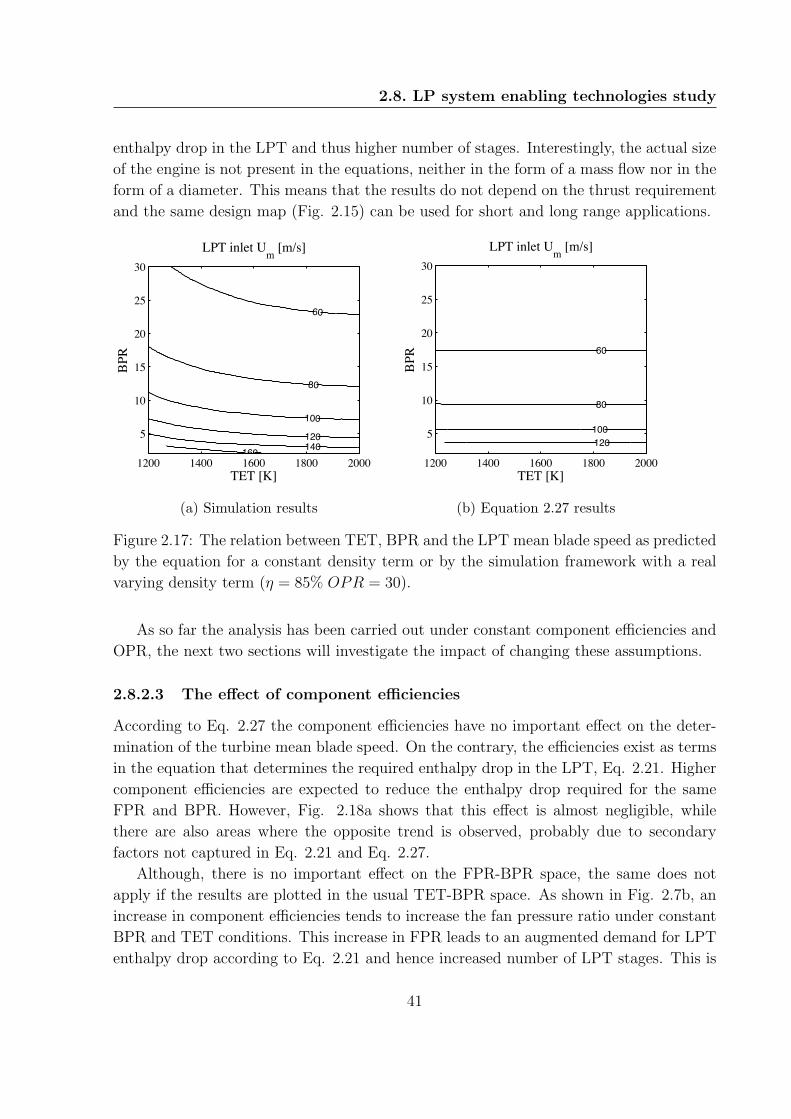
2.8. LP system enabling technologies study

enthalpy drop in the LPT and thus higher number of stages. Interestingly, the actual size

of the engine is not present in the equations, neither in the form of a mass flow nor in the

form of a diameter. This means that the results do not depend on the thrust requirement

and the same design map (Fig. 2.15) can be used for short and long range applications.

1200 1400 1600 1800 2000

5

10

15

20

25

30

TET [K]

BPR

LPT inlet Um [m/s]

60

80

100

120140160

(a) Simulation results

1200 1400 1600 1800 2000

5

10

15

20

25

30

TET [K]

BPR

LPT inlet Um [m/s]

60

80

100120

(b) Equation 2.27 results

Figure 2.17: The relation between TET, BPR and the LPT mean blade speed as predicted

by the equation for a constant density term or by the simulation framework with a real

varying density term (η = 85% OPR = 30).

As so far the analysis has been carried out under constant component efficiencies and

OPR, the next two sections will investigate the impact of changing these assumptions.

2.8.2.3 The effect of component efficiencies

According to Eq. 2.27 the component efficiencies have no important effect on the deter-

mination of the turbine mean blade speed. On the contrary, the efficiencies exist as terms

in the equation that determines the required enthalpy drop in the LPT, Eq. 2.21. Higher

component efficiencies are expected to reduce the enthalpy drop required for the same

FPR and BPR. However, Fig. 2.18a shows that this effect is almost negligible, while

there are also areas where the opposite trend is observed, probably due to secondary

factors not captured in Eq. 2.21 and Eq. 2.27.

Although, there is no important effect on the FPR-BPR space, the same does not

apply if the results are plotted in the usual TET-BPR space. As shown in Fig. 2.7b, an

increase in component efficiencies tends to increase the fan pressure ratio under constant

BPR and TET conditions. This increase in FPR leads to an augmented demand for LPT

enthalpy drop according to Eq. 2.21 and hence increased number of LPT stages. This is

41

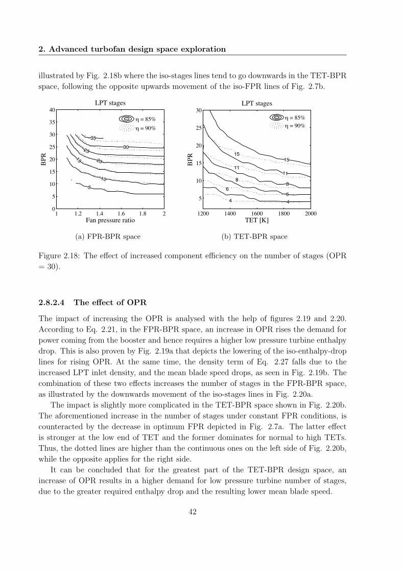
2. Advanced turbofan design space exploration

illustrated by Fig. 2.18b where the iso-stages lines tend to go downwards in the TET-BPR

space, following the opposite upwards movement of the iso-FPR lines of Fig. 2.7b.

1 1.2 1.4 1.6 1.8 20

5

10

15

20

25

30

35

40

Fan pressure ratio

BPR

LPT stages

510

15 20

2530

35

d = 85%d = 90%

(a) FPR-BPR space

1200 1400 1600 1800 2000

5

10

15

20

25

30

TET [K]

BPR

LPT stages

46

8

11

15

4

6

8

11

15

d = 85%d = 90%

(b) TET-BPR space

Figure 2.18: The effect of increased component efficiency on the number of stages (OPR

= 30).

2.8.2.4 The effect of OPR

The impact of increasing the OPR is analysed with the help of figures 2.19 and 2.20.

According to Eq. 2.21, in the FPR-BPR space, an increase in OPR rises the demand for

power coming from the booster and hence requires a higher low pressure turbine enthalpy

drop. This is also proven by Fig. 2.19a that depicts the lowering of the iso-enthalpy-drop

lines for rising OPR. At the same time, the density term of Eq. 2.27 falls due to the

increased LPT inlet density, and the mean blade speed drops, as seen in Fig. 2.19b. The

combination of these two effects increases the number of stages in the FPR-BPR space,

as illustrated by the downwards movement of the iso-stages lines in Fig. 2.20a.

The impact is slightly more complicated in the TET-BPR space shown in Fig. 2.20b.

The aforementioned increase in the number of stages under constant FPR conditions, is

counteracted by the decrease in optimum FPR depicted in Fig. 2.7a. The latter effect

is stronger at the low end of TET and the former dominates for normal to high TETs.

Thus, the dotted lines are higher than the continuous ones on the left side of Fig. 2.20b,

while the opposite applies for the right side.

It can be concluded that for the greatest part of the TET-BPR design space, an

increase of OPR results in a higher demand for low pressure turbine number of stages,

due to the greater required enthalpy drop and the resulting lower mean blade speed.

42

2.8. LP system enabling technologies study

1 1.2 1.4 1.6 1.8 20

5

10

15

20

25

30

Fan pressure ratio

BPR

LPT enthalpy drop [J/kg]

200000

300000

400000500000

OPR = 30OPR = 50

(a)

1 1.2 1.4 1.6 1.8 20

5

10

15

20

Fan pressure ratioBP

R

LPT inlet Um [m/s]

80

100

80100

140

OPR = 30OPR = 50

(b)

Figure 2.19: The effect of increased OPR on the LPT enthalpy drop and mean blade

speed (η = 85%).

1 1.2 1.4 1.6 1.8 20

5

10

15

20

25

30

35

40

Fan pressure ratio

BPR

LPT stages

510

20

5

10

10

20

OPR = 30OPR = 50

(a) FPR-BPR space

1200 1400 1600 1800 2000

5

10

15

20

25

30

TET [K]

BPR

LPT stages

46

8

11

15

15

11

86

4

OPR = 30OPR = 50

(b) TET-BPR space

Figure 2.20: The effect of increased OPR on the number of stages (η = 85%).

43

2. Advanced turbofan design space exploration

2.9 Installed performance results

The title installed performance comprises all the previously analysed results in order to

create a design space map that shows the position of the optimum short and long range

engines and the technologies required to implement them. The preliminary design code

has already calculated the weight of the engine and its dimensions, which are subsequently

used in order to estimate its drag (see section 2.4.3). Table 2.3 lists the assumptions used

in the installed performance analysis as discussed in section 2.4.3, with typical ranges for

short and long range missions. A set of higher technology specifications is given in table 2.4

corresponding to a technology improvement typically taking place within approximately

20 years [10, 17, 62–67].

Table 2.3: Installed performance calculation assumptions

Parameter Value

Short range 3000 km

Long range 14000 km

Drag coefficient CD 0.002

Drag interference factor κi 1.2

Nacelle density factor κnac 24.88 kg/m2

Cowl L/D ratio 1.5

Table 2.4: Low weight and drag case assumptions

Parameter Value

Drag coefficient CD 0.001

Drag interference factor κi 1.2

Nacelle density factor κnac 20 kg/m2

Cowl L/D ratio 1

Fan & LPT weight -50%

Other components weight -15%

The design space maps for the short and long range missions are depicted in Fig. 2.21

and 2.22 respectively. Each sub-figure shows the variation of the range factor Kr in the

TET-BPR design space, for given component efficiencies and OPR. The sub-figures 2.21d

and 2.22d add the case of improved installation technology, according to the assumptions

44

2.9. Installed performance results

of table 2.4. The continuous lines represent the lines of equal specific thrust, the dashed

lines show the number of LPT stages required and the dash-dot lines the TET at take-off

conditions. The requirement for variable fan area as function of FPR, shown in Fig. 2.14c,

has been translated into a function of ST using Fig. 2.8. This results in a requirement

for 10% fan nozzle area increase for engines with ST lower than 130 m/s and 20% for

the ones with ST lower than 80 m/s. Only the iso-stages line of 7 and 8 LPT stages are

depicted, as after this threshold the number of LPT parts would be excessively high and

a geared configuration would be possibly required.

As a preliminary step of this results analysis, table 2.5 presents the sensitivity of

the range factor to the variation of SFC, drag and weight for the short and long range

mission. The baseline reference values correspond to the square points of Fig. 2.21a and

2.22a for the short and long range engine respectively. As expected, the SFC dominates

the installed performance, with a higher impact for the long range mission where the vast

majority of the fuel is consumed at cruise. The weight has the second greatest influence,

especially for the short range mission where the exchange rate is almost three times higher

than the long range one. The influence of drag is much less, possibly due to optimistic

assumptions in the calculation of nacelle drag.

2.9.1 Validation

The square point on Fig. 2.21a represents the baseline optimum, typical of engines cur-

rently in service in the short range market. With a bypass ratio around 5 and a diameter

around 1.5m (Fig. 2.23), it is not far from the data published in Janes for the CFM

and V2500 engines [62]. Furthermore, Fig. 2.21d shows that in the advanced installation

technology case, the resulting optimum bypass ratio of about 8 (circle point) and the

corresponding optimum diameter of about 1.7m are not far from the claimed values of

the new LEAP engine [62].

Similarly, for the long range baseline case of Fig. 2.22a (square point), the bypass

ratio of about 7 and the diameter of 3m are again not far from the values of the current

GE90 and RR Trent 892 engines [17, 62].

In both short and long range engines, the turbine entry temperature is selected in

order to have a good compromise and agreement with the published bypass ratios [62]

and the estimated current and future levels of TET [6, 8, 29, 36, 37, 62].

Hence, it can be claimed that the used models and assumptions lead to realistic solu-

tions and can be safely used in order to extract further conclusions.

2.9.2 Optimum specific thrust

The first observation that can be made for 2.21a, is that the optimum short range ST

is around 260 m/s, which is much lower than the uninstalled optimum of 75 m/s (Fig.

45

2. Advanced turbofan design space exploration

2.9a). This significant difference between the two solutions is attributed to the inclusion

of the engine weight and drag effects, which penalise higher diameter solutions. Secondly,

it is readily observed from all the sub-cases of Fig. 2.21 that the optimum ST does not

depend on the engine OPR or component efficiencies. It is only a function of the installed

performance characteristics, which include the mission range and the variation of the

engine weight and drag with ST. As seen in sub-figure 2.21d, a lower optimum ST can be

attained only when the installation technology is improved.

Along the same lines, Fig. 2.22a shows that the optimum specific thrust for the

baseline long range engine is significantly lower, with a value of 180 m/s. The corre-

sponding advanced installation technology optimum falls to 142 m/s according to Fig.

2.22d. These significantly lower values of optimum ST are readily explained by the range

factor exchange factors of table 2.5, which show the higher important of SFC for long

range applications.

The above observations confirm the statements by Young [38] and Guha [29] regard-

ing the optimisation of ST, which should be done independently from the other engine

parameters and in close cooperation with the aircraft manufacturer.

2.9.3 TET limitation

Having chosen the specific thrust following the installed performance considerations, the

design can then move on an iso-ST line in compliance with the constraints of TET.

Applying a limit on the maximum TET at take-off immediately fixes the design point

BPR. This is why the core of the engine is sized at take-off. The diameter is fixed by

the selection of specific thrust and then the maximum allowable temperature gives the

maximum allowable BPR and thus the minimum possible core size. The same limit on

BPR can be applied by the top-of-climb temperature if it is higher than the take-off one,

or if it is high enough to compromise the creep life of the engine.

2.9.4 HPC delivery temperature limitation

According to the analysis presented in section 2.7.2.2, a limitation on the high pressure

compressor delivery temperature must also be taken into account. With the optimum

specific thrust being defined by the installed performance, the only way to control the

T3 at take-off is via the overall pressure ratio for a given level of component efficiencies.

Figures 2.12a and 2.21a show that current short range engines do not face an important

restriction (the current levels of OPR being about 30), but a future increase of OPR up

to 40 can only be brought about with a parallel increase of their compressor efficiency

(Fig. 2.12b). On the other hand, a future amelioration of the installation technology

would further decrease the optimum ST, relieving this way the HPC exit temperatures at

take-off as shown by Fig. 2.12.

46

2.9. Installed performance results

The long range engines are located closer to the T3 limit due to their higher overall

pressure ratios. Figure 2.12a shows that with a polytropic efficiency of 90% and using the

optimum ST of 180 m/s (Fig. 2.22a), the attained level of T3 would be higher than 950

K but still lower than 1000 K. This is an indication that current long range engines have

probably compressor polytropic efficiencies higher than 90% or cruise OPR less than 40.

In fact, these hypotheses are confirmed by the Trent 892 model of Jackson [17], which

employs polytropic efficiencies of 92%, 92.5% and 88.6% for the fan hub, IPC and HPC

respectively. With this set of efficiencies and with a cruise OPR level of 33 (versus 40

assumed here) Jackson’s model generates a T3 of 910 K at take-off. This value is already

very close to the limit, proving the point that long range engines OPR is probably limited

by the T3 at take-off.

Once more, a possible future increase of OPR from 40 to 50 will be enabled by higher

polytropic efficiencies, better materials and the lower optimum levels of specific thrust

due to better installation technology.

2.9.5 Variable area fan nozzle

The results of Fig. 2.21 show that no variable fan nozzles are needed for the short

range engine, even for the decreased optimum ST of 215 m/s (Fig. 2.21d). A geared

configuration would probably result in a more aggressive relation between weight and

diameter with the optimum translated towards lower ST. For example, if one follows the

iso-TET@TO line of 2000 K up to the value of BPR equal to 13 (maximum value claimed

in Janes for the GTF of Pratt & Whitney), they would end up with a design much closer

to the requirement for variable fan nozzle.

On the other hand, the inherently lower ST long range engines are much closer to the

limit of fixed geometry nozzle. According to Fig. 2.22d, the next generation of long range

engines will most probably need the introduction of such a technology in order to ensure

the safe operation of the fan at take-off.

The impact of the variable area fan nozzle on the selection of the optimum solution

will be commented in section 2.9.7 with the help of the calculated performance exchange

rates.

2.9.6 Gearbox

Figure 2.21a shows that the baseline short range engines are well inside the conventional

turbofan design area, with a number of LPT stages below 8. A higher design turbine

entry temperature, a higher OPR (Fig. 2.21b) or a higher level of component efficiencies

(Fig. 2.21c) would not change the optimum ST but they would move the iso-stages

lines downwards, compressing this way the available conventional turbofan area. The

explanation of these trends has already been given in section 2.8.2. Finally, the lower

47

2. Advanced turbofan design space exploration

optimum ST enabled by a low drag and weight installation would position the optimum

design to the limit of the non-geared space (square point Fig. 2.21d) or even slightly

inside the geared configuration area if the TET is also increased (circle point Fig. 2.21d).

In reality the circle point of Fig. 2.21d could be still implemented without a gearbox if the

number of stages was reduced to 7-8, 7 being the value claimed for the LEAP engine [68].

A possible way of achieving this is indicated by Eq. 2.26, which shows that an increase

of the mean LPT radius could lead to a higher blade speed and a consequent decrease in

the number of stages.

The schematic of GE-90 published in Janes [62] clearly shows the implementation of

this practice, with the LPT inlet radius being significantly higher than the HPT exit. If

a fictitious GE-90 engine was approximately positioned on the design map of Fig. 2.22a,

using a value of TET at take-off equal to 1865 K and BPR equal to 8.1 as claimed in

Janes [62], the resulting number of stages would be about 8. In reality the engine has

only 6 stages, difference which is attributed in this study’s design assumption of a hub

radius which is constant and equal to the exit of the HPT.

Notwithstanding the above simplifying assumption regarding the LPT radius, it is

evident from Fig. 2.22 that long range engines are much closer to the limit of non-geared

configurations. This is not the result of a size effect between high and low thrust engines,

but the outcome of the lower optimum specific thrusts inherent in long range applications.

Figure 2.22d clearly illustrates that if the installation technology improves, the new long

range optimum will move well inside the geared configuration space. This effect will be

slightly delayed for three spool configurations which tend to have an inherently lower

number of stages in the LPT (according to Jackson [17] the RR Trent 892 has 5 LPT

stages versus the 6 of the GE-90).

In closing, it must be reminded that the geared configuration itself is likely to have

a more aggressive relation between the engine diameter and its weight. This means that

the engine weight would increase slower with diameter for a geared configuration than

for a conventional. This argument is based on Riegler’s argument [10] that for the same

thermodynamic cycle, a geared configuration would have an LPT 40% lighter. Another

proof that this argument might be correct is the higher diameters proposed by Pratt &

Whitney relative to the ones proposed for the LEAP engines for the same applications

[68]. This line of thought leads to the conclusion that a geared configuration will probably

have a lower optimum ST, unlocking this way a further SFC benefit by better restraining

the installation losses.

2.9.7 Exchange rates

This exchange rate analysis attempts to quantify all the design trends mentioned in the

previous sections. Figure 2.24 shows the percentage change of SFC and Kr for given

48

2.9. Installed performance results

changes of OPR, TET, installation technology and specific thrust. The results are re-

peated for the short and long range engine, for component efficiencies of 90 and 95 percent.

The short range baseline engine corresponds to the square point of Fig. 2.21a and the long

range on the square point of Fig. 2.22a. The specific thrust and diameter are considered

constant for all the step changes apart from the last which considers the reduction of

specific thrust. As shown in Fig. 2.24, the improvement of component efficiencies brings

in its own a significant improvement of performance and this a proof that engine design

will definitely attempt to follow this path. Finally, with the drag playing a negligible role,

the differences between the SFC and the Kr can be explained using the variation in SFC

and weight and the exchange rates shown in table 2.5.

2.9.7.1 Overall pressure ratio

For all the cases of Fig. 2.24, the increase of OPR leads to a decrease in SFC with a lesser

decrease in Kr due to the variations of engine weight. The SFC improvement is higher

for the short range engine due to the lower baseline OPR of 30. This occurs because

the curve between OPR and SFC demonstrates an asymptotic trend as OPR increases.

Hence, a delta applied on a low OPR has a greater impact than the same delta applied on

a higher OPR. Along the same lines, the improvement is higher for high efficiencies than

for low, due to the shifting of the optimum OPR towards higher values as the efficiencies

increase [27].

Regarding the installed performance, the preliminary design code predicts slight re-

ductions of weight for the short range engine, while the opposite occurs for the long range.

Although more investigation is required, this effect could be probably attributed to the

lower fan weight as the OPR increases and the core gets bigger with a constant fan diam-

eter. In the long range case, the opposite effect of increasing core size and engine length

dominates, the weight increases and this widens the gap between SFC and Kr.

In summary, an increase of 25% in OPR can improve the SFC by 1-3% for a short

range engine and by about 1% for a long range one. Depending on the variations of engine

weight this can be translated in an improvement of fuel burn by 1-1.5% for the short range

engine and up to 1% for the long range one.

2.9.7.2 Turbine entry temperature and Variable area fan nozzle

An increase of TET by 100 K brings at all cases an SFC improvement and an approxi-

mately equal or even higher improvement of fuel burn (proportional to Kr). This happens

due to the reduction of weight due to the smaller size of the hotter engine core. The SFC

improvement is lower for the higher efficiencies case due to the lower levels of the optimum

TET, as described in section 2.2. Similarly, the SFC improvement is higher for the long

range engine due to its higher OPR, which shifts the optimum TET towards higher values

49

2. Advanced turbofan design space exploration

[27]. The beneficial reduction of weight is more evident in the short range case, where the

Kr improves more than the SFC. This happens because of the higher impact of engine

weight on the short range fuel burn as proven by table 2.5.

As a general comment, the exchange rates of TET confirm the arguments of Kurzke

[27], concerning the limited prospects of further TET increases. Especially if the com-

ponent efficiencies continue to increase, the positive impact of TET will be extinguished

or even reversed. This can be aggravated more if the negative effects of small size and

higher cooling flows are taken into account.

In the light of the above observations, the benefits of introducing a variable area fan

nozzle as a means of achieving a smaller and hotter core does not seem appealing. It

has been shown in section 2.8.1 that a VFN could help increase the cruise TET by 15-

50K. According to Fig. 2.24 this can bring a maximum Kr improvement of 1% which

could easily reduce to zero if the aforementioned negative effects are taken into account.

Considering the added complexity of a variable nozzle, its introduction is not justified

from the results shown here.

2.9.7.3 Improved installation technology and lower specific thrust

The effect of improving the installation technology by reducing the engine drag and weight

is immediately apparent from all the cases of Fig. 2.24. Without changing the engine

cycle - hence SFC being constant - this technology step can deliver a fuel reduction of up

to 13 and 7 percent for the short and long range engines respectively. This is why all the

engine manufacturers invest a lot in composite and lightweight materials.

Moreover, this technology improvement can unlock a further 4.5 to 6.5 percent SFC

improvement through a lower optimum specific thrust. The low value of 4.5% corresponds

to the long range which already has a low ST and thus is less affected by the technology

step change. The exact Kr potential of the 4.5-6.5% SFC improvement depends on the

weight characteristics of the engine. Figure 2.24 demonstrates that it is easier to release

this SFC potential in the long range case where efficiency is more important than en-

gine weight. Based on the assumptions of this study, the reduction of ST could bring

a maximum Kr reduction of 1.7 and 2.5 percent for the short and long range engines

respectively.

The potential benefits of lighter geared configuration also become apparent. If a geared

configuration could ”soften” the relation between engine diameter and weight, the gap

between SFC and Kr would further diminish. The exact amount of this potential can

only be quantified with a more detailed engine design investigation, which is outside the

scope of this work.

50

2.9. Installed performance results

2.9.8 Some possible design paths

2.9.8.1 Short range engine

Starting from the baseline square point of Fig. 2.21a, the design will certainly go towards

higher component efficiencies and lower installation losses. This is justified by the sig-

nificant exchange rates shown in Fig. 2.24 for these two step changes, delivering a fuel

decrease of up to 23%. The thermal efficiency will be then improved by increasing the

OPR, with the T3 being under control due to the higher compressor efficiencies. This

would bring another 1.7% of fuel reduction. The specific thrust would be decreased mov-

ing to the new optimum of 215 m/s, reducing thereby the fuel by 1.2% (square point Fig.

2.21d). At this point the design is at the edge of the conventional non-geared design. A

further increase in TET would be probably avoided, as it would lead to negligible fuel

reductions (Fig. 2.24b) and would move the design towards the more complex geared

configuration (circle point of Fig. 2.21d). The fuel burn difference between the baseline

engine and the final one, could reach the total of 25.9%. In a most likely scenario where

only half of the component and installation improvement were achieved, this fuel reduc-

tion would reduce down to 14.4%, which is close to the claimed improvement between the

LEAP and the CFM56 engines [62, 68].

2.9.8.2 Long range engine

Following the same process for the long range engine, and starting again from the square

point of Fig. 2.22a, the improved efficiencies and installation technology deliver a fuel

decrease up to 19%. The increase of OPR would bring a fuel burn reduction of 0.8%

and the new optimum ST of 142 m/s another 1.5%. At this point the solution lies in

the triangle point of Fig. 2.22d, well inside the geared configuration space. A higher

TET could potentially lead to a maximum improvement of 0.8%, which however could

compromise the creep life of the engine.

At this point it would be quite interesting to contemplate the scenario where a geared

configuration were to be avoided at all cost. In that case the design would have to move

to a significantly lower TET at the square point of Fig. 2.22d. This would result in a

fuel burn about 2% worse, but with a TET lower by 200 K and without the need for

a gearbox. The fuel burn increase of 2% could be even smaller, if the reduced cooling

requirement and the lower component size effects were taken into account. To sum up,

if all the aforementioned improvements were introduced, the final engine (circle point in

Fig. 2.22d) would have a fuel burn 22.1% lower than the baseline. Once again, in the

most likely scenario where only half the improvement of efficiencies and installation were

to take place, the reduction would reduce to 12.6%. If no gearbox were to be used, the

maximum benefit would reduce to 19.3% and the most likely to 9.8%; i.e. a difference

of 2.8% between the conventional and the geared configuration. This difference would be

51

2. Advanced turbofan design space exploration

a bit higher, if the geared configuration resulted in a lower weight for the circle point of

2.22d, relative to the weight calculated here using the non-geared assumptions.

2.10 Conclusions

The aim of this chapter was to create a design space that shows the position of the

optimum short and long range engines and to demonstrate which low pressure system

technologies are required for their implementation.

An extensive literature review was conducted in order to clarify the parameters that

drive engine efficiency, understand the current design trends and the enabling technologies

required. The variable area fan nozzles and the geared architecture are the two technolo-

gies identified as the natural extension of the current design trends of turbofan engines.

An analysis and optimisation framework was set up, comprising models that predict the

engine performance, the dimensions and weight, the drag, and the installed performance.

The engine performance model has been updated in order to correctly simulate the com-

bustor balance, which results in the existence of a turbine entry temperature optimum.

The principles of engine preliminary design were studied and translated into a numerical

problem formulation using the created optimisation framework. The analysis was focused

on a two-spool turbofan configuration for a short and a long range mission.

The uninstalled performance analysis established and clarified the relations between

the specific thrust, the bypass ratio, the turbine entry temperature, the overall pressure

ratio, the component efficiencies and the optimum value of the fan pressure ratio. The

specific thrust was found as the parameter dominating the design, for it defines the fan

pressure ratio, the propulsive efficiency, the engine diameter and the relation between

the in-flight and the take-off turbine entry temperature. A lower specific thrust results

in a cooler engine at take-off for a fixed value of turbine entry temperature at top-of-

climb. ”Relieving” the engine power setting at take-off also allows higher overall pressure

ratios to be used at top-of-climb, improving thereby the engine thermal efficiency, without

reaching excessive temperatures at the exit of the high-pressure compressor.

The requirement for a variable area fan nozzle was connected with the design fan

pressure ratio of the engine. A relation was also found to exist between the required area

increase and the fan pressure ratio, confirming this way the results of Jackson [17]. The

strong relation between the fan pressure ratio and the engine specific thrust results in a

law that defines the required area increase according to the specific thrust. Engines with

specific thrust lower than 130 m/s require a nozzle area increase of 10%, while an increase

of 20% is needed for engines with specific thrust lower than 80 m/s. The variable area fan

nozzle can also be used in order to achieve the same take-off thrust with a lower turbine

entry temperature, enabling this way the design of engines with cores smaller and hotter

by up to 50 K.

52

2.10. Conclusions

The gearbox study related the number of low pressure turbine stages to the thermody-

namic cycle characteristics. The fan pressure ratio and the bypass ratio are the dominant

parameters. Increased bypass ratios increase the number of stages, due to the lower tur-

bine blade speeds and the higher required turbine enthalpy drop. Increased fan pressure

ratios increase the number of stages due to the higher fan work that increases the required

turbine enthalpy drop. Increased overall pressure ratio and component efficiencies com-

press the conventional turbofan design space by increasing the number of stages needed

for the same turbine entry temperature and bypass ratio. No size effect is found to exist

and thus two engines sharing the same cycle and design but with different thrusts will

have the same number of low pressure turbine stages.

The installed performance integrates all the results in order to create the final design

space maps. The results showed good agreement against current and near future engines

of the short and long range market. The optimum specific thrust is determined only by the

installation characteristics and it is lower for engines with longer range, lower weight and

lower drag. Having defined the specific thrust through the installed performance trade-

offs, the limits of turbine entry temperature subsequently impose the minimum allowable

engine core size. The optimum value of specific thrust, also fixes the maximum allowable

design overall pressure ratio with respect to the compressor exit temperature restrictions

at take-off.

The created design space maps show that the variable area fan nozzle will be probably

required for the next generation of long range engines, due to their low optimum specific

thrust. The gearbox will be also probably needed for both short and long range engines, as

the lower specific thrust, higher overall pressure ratio and improved component efficiencies

are pushing the conventional turbofan to its limits. The long range engines have the

priority as they feature higher overall pressure ratios and lower specific thrusts.

Only mediocre improvements in thermal efficiency can be achieved by increasing the

overall pressure ratio and turbine entry temperature relative to today’s levels, confirming

the statements of Kurzke [27, 36]. Increasing the overall pressure ratio by 25% can deliver

a fuel burn improvement of 1.7 and 0.8 percent for the short and long range engines

respectively. Increasing the TET by 100 K leads to almost no improvement for the short

range and to a 0.8% improvement for the long range engine. The OPR benefit increases

for higher component efficiencies, while the opposite happens with TET. The above trends

mean that there is probably no benefit in using the variable area fan nozzle in order to

achieve a smaller and hotter core design.

In an extreme scenario the turbine entry temperatures could even decrease by 200 K

relative to today’s levels, in order to decrease the bypass ratio and avoid completely the

introduction of a gearbox. This scenario could result in an engine with potentially lower

maintenance costs, lower cooling requirements and lower component size effects, without

an excessive efficiency penalty as long as its weight is controlled.

53

2. Advanced turbofan design space exploration

Future fuel reductions are most likely to be sought by improvements of component

efficiencies, reduced engine weight and drag, and lower specific thrusts.

54

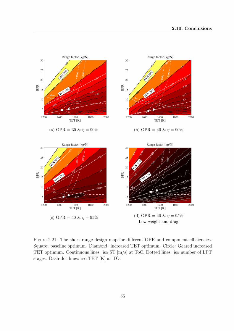
2.10. Conclusions

1200 1400 1600 1800 2000

5

10

15

20

25

30

TET [K]

BPR

Range factor [kg/N]

78

VFN 20

%0.6

0.5

VFN 10%

0.40.35

0.330.32

0.31

80

130

260

1900

2000

(a) OPR = 30 & η = 90%

1200 1400 1600 1800 2000

5

10

15

20

25

30

TET [K]BP

R

Range factor [kg/N]

87

VFN 20

%

VFN 10%

0.6

0.5

0.4

0.35

0.33

0.31

0.3

80

130

260

1900 20

00

(b) OPR = 40 & η = 90%

1200 1400 1600 1800 2000

5

10

15

20

25

30

TET [K]

BPR

Range factor [kg/N]

VFN 20

%

VFN 10%

0.6

0.5

0.4

0.35 0.3

0.28

80

130

260

1900 20

00

87

0.27

(c) OPR = 40 & η = 95%

1200 1400 1600 1800 2000

5

10

15

20

25

30

TET [K]

BPR

87

VFN 20

%

VFN 10%

Range factor [kg/N]

0.4

0.35

0.3

0.28

0.26

0.250.245

0.235

1900

2000

80

130

215

260

0.24

(d) OPR = 40 & η = 95%Low weight and drag

Figure 2.21: The short range design map for different OPR and component efficiencies.

Square: baseline optimum. Diamond: increased TET optimum. Circle: Geared increased

TET optimum. Continuous lines: iso ST [m/s] at ToC. Dotted lines: iso number of LPT

stages. Dash-dot lines: iso TET [K] at TO.

55

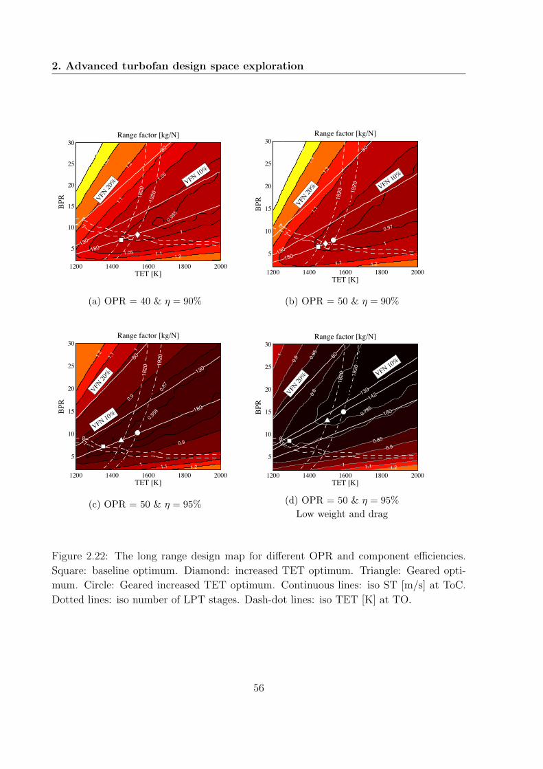
2. Advanced turbofan design space exploration

1200 1400 1600 1800 2000

5

10

15

20

25

30

TET [K]

BPR

Range factor [kg/N]

87

VFN 20

% VFN 10%

1.6

1.4 1.2

1.1

1.05

1.05 1.1 1.2

1

0.985

80

130180

1820

1920

(a) OPR = 40 & η = 90%

1200 1400 1600 1800 2000

5

10

15

20

25

30

TET [K]

BPR

Range factor [kg/N]

87

VFN 20

% VFN 10%

1.6

1.4

1.2

1.1

1.1 1.2

1

0.97

80

130180

1820 19

20

(b) OPR = 50 & η = 90%

1200 1400 1600 1800 2000

5

10

15

20

25

30

TET [K]

BPR

Range factor [kg/N]

87

VFN 20

%

VFN 10%

1.2

1.1

1

0.9

0.87

0.858

0.9

1 1.1 1.2

80

130

180

1820

1920

(c) OPR = 50 & η = 95%

1200 1400 1600 1800 2000

5

10

15

20

25

30

TET [K]

BPR

Range factor [kg/N]

87

VFN 20

% VFN 10%

1

0.9 0.8

50.

8

0.785

0.850.9

1 1.1 1.2

80

130142

180

1820 19

20

(d) OPR = 50 & η = 95%Low weight and drag

Figure 2.22: The long range design map for different OPR and component efficiencies.

Square: baseline optimum. Diamond: increased TET optimum. Triangle: Geared opti-

mum. Circle: Geared increased TET optimum. Continuous lines: iso ST [m/s] at ToC.

Dotted lines: iso number of LPT stages. Dash-dot lines: iso TET [K] at TO.

56

2.10. Conclusions

Table 2.5: Range factor engine parameters exchange rates

Delta parameter Delta Kr SR Delta Kr LR

-1% SFC -0.68% -0.89%

-1% Drag -0.01% -0.02%

-1% Weight -0.33% -0.13%

0 100 200 300 400 500 6000

1

2

3

4

5

6

7

8

ST [m/s]

Fan

diam

eter

[m]

T = 86 kN

T = 26 kN

Figure 2.23: The relation between the specific thrust and the fan tip diameter for the

short and long range engine (η = 90% OPR = 40).

57

2. Advanced turbofan design space exploration

-15 -14 -13 -12 -11 -10 -9 -8 -7 -6 -5 -4 -3 -2 -1 0

Baseline OPR +25%

TET +100K

Low drag & weight

ST -20%

Del

ta [%

]

Delta SFC Delta K

(a) Short range & η = 90%

-15 -14 -13 -12 -11 -10 -9 -8 -7 -6 -5 -4 -3 -2 -1 0

ETA +5pt

OPR +25%

TET +100K

Low drag & weight

ST -20%

Del

ta [%

]

Delta SFC Delta K

(b) Short range & η = 95%

-15 -14 -13 -12 -11 -10 -9 -8 -7 -6 -5 -4 -3 -2 -1 0

Baseline OPR +25%

TET +100K

Low drag & weight

ST -20%

Del

ta [%

]

Delta SFC Delta K

(c) Long range & η = 90%

-15 -14 -13 -12 -11 -10 -9 -8 -7 -6 -5 -4 -3 -2 -1 0

ETA +5pt

OPR +25%

TET +100K

Low drag & weight

ST -20%

Del

ta [%

]

Delta SFC Delta K

(d) Long range & η = 95%

Figure 2.24: SFC and range factor (K) exchange rates for different missions and com-

ponent efficiencies. The short and long range mission baseline engines correspond to the

square symbols of Fig. 2.21a and Fig. 2.22a respectively. The low weight and drag case

corresponds to: -50% drag and -35% weight for the SR and -45% for the LR.

58

Chapter 3

Secondary power extraction effects

3.1 Introduction

Aircraft engines are not merely a source of propulsive power but they also provide for

the secondary power needs of the aircraft. Power is extracted from the engine core in

the form of compressed air and shaft power in order to satisfy the requirements of the

pneumatic, hydraulic, electric and cabin pressurization aircraft systems. The extraction

of secondary power imposes an increase of about 1-4% in fuel consumption [4]. This

chapter investigates how this fuel efficiency penalty varies for different engine designs by

relating the main engine thermodynamic parameters with the magnitude of the penalty.

The analysis presented here essentially complements the results presented in the previous

chapter by adding the engine size effect of given bleed and power off-takes.

The effects of secondary power extraction were brought under investigation after the

1970s oil crises. The replacement of conventional secondary systems by one globally

optimized all-electric system was contemplated in several studies published in the past

[69–71]. Concerns were also focused on whether secondary power extraction would be

heavier a burden for future high bypass ratio engines, due to their smaller engine cores

[28, 69, 72].

Matching the engine for normal off-takes, which remain proportionally constant along

the flight envelope, is a common practice to reduce the associated penalties [4, 73]. How-

ever there is still no single answer as to whether higher bypass ratio engines would suffer

greater penalties than today’s engines [4, 28, 69, 74]. Peacock stressed that the way the

engine is resized to accommodate the off-takes plays a significant role in answering that

question. The required resizing of the engine can be carried out either by keeping a con-

stant diameter and specific thrust, while allowing the core size to float [75], or by keeping

the bypass ratio constant and vary the size of the whole engine [76]. In that context,

Peacock argued that if the first resizing method was employed no greater penalties would

59

3. Secondary power extraction effects

be imposed for higher bypass ratio engines, contrary to the second method where the

penalties would increase.

Nowadays, secondary power extraction is still a current issue of research and discussion

due to the continuous pursuit for more efficient aircraft/engines [12, 13]. Researchers

continue to investigate the efficiency of different secondary power systems configurations

[11, 14–16], and how this affects the whole aircraft performance [77].

This work aims to identify how secondary power extraction penalties relate to dif-

ferent engine thermodynamic designs. This entails testing the hypothesis that future

engines with lower specific thrusts will suffer greater fuel efficiency penalties. An ana-

lytical method is used in order to derive expressions that relate the size of the off-take

penalties to the design parameters of the engine. The analysis is based on the fundamen-

tals of gas turbine aero engine efficiency and thermodynamics, and applies to the cruise

design point of the engine, where fuel consumption is of utmost importance. The derived

equations include design parameters that are known in the early preliminary design stages,

and their validity is tested against Turbomatch. The conducted analysis offers physical

insight on the parameters that drive the off-take penalties and has also been used to study

the differences between the two resizing methods mentioned before. Finally, the devel-

oped analytical relations constitute a fast calculation tool in the hands of aircraft, engine,

and secondary systems designers; any change in the characteristics of the engine and the

secondary power systems can be translated to a fuel burn change, and subsequently, by

applying the Breguet equation [32], to an aircraft range change.

3.2 Engine Core Efficiency Analysis

The determination of the secondary power extraction penalties is based upon estimating

the changes in the individual efficiencies when bleed air or shaft power are taken off the

engine. The enthalpy-entropy diagram will be used as a basis for the analysis, in order

to determine the changes in the core efficiency. It is emphasized that the analysis applies

to the design point of the engine, where the turbine entry temperature, overall pressure

ratio and component efficiencies are kept constant.

The starting point will be a clean engine with zero bleed and shaft power off-takes.

Then, shaft power and bleed air will be taken off the engine, with everything else kept

constant. This will result in a reduction in thrust, which, for constant fuel inflow, will be

translated to an equivalent reduction in efficiency. Therefore, to keep the thrust constant

at its design value the engine has to be resized, and the reduction in efficiency will then

be manifested as an increase in fuel flow.

60

3.2. Engine Core Efficiency Analysis

3.2.1 Shaft power off-takes

Figure 3.1 shows how the extraction of shaft power affects the enthalpy-entropy diagram.

The pressure ratio of the high-pressure turbine has to increase to cope with the increased

demand in power and thus, everything else kept constant, the pressure at the exit of the

core will fall. Consequently, the enthalpy produced by the core will also fall from ∆hcp to

∆h∗cp according to Eq. 3.1.

h05

h*5

h04

s*5s5

h*05

h*CP

Burner exit

Core exit

Core exit withoff takes

Ambientpressure

s4

h [kJ/kg]

s [kJ/kgK]

h5

hCP

h*05

Figure 3.1: Enthalpy-entropy diagram at the core exit with and without off-takes.

∆h∗cp = ∆hcp −∆h∗05 − (h∗5 − h5) (3.1)

where ∆h∗cp represents the enthalpy produced by the core when secondary shaft power

is extracted and ∆h∗05 the enthalpy extracted as secondary power. If the losses due to the

expansion to higher ambient temperature (h∗5 − h5) are assumed equal to zero, Eq. 3.1

can be written in power terms as:

P ∗cp = Pcp − Ppo (3.2)

where Ppo = Wh∆h∗05 is the extracted shaft power. With the fuel flow kept constant,

the above power drop will result in an equivalent drop in the efficiency of the core as

61

3. Secondary power extraction effects

described by Eq. 3.3, or by Eq. 3.4, relative to the clean engine efficiency.

η∗co =P ∗cp

WffFCV=Pcp − PpoWffFCV

(3.3)

η∗coηco

= 1− PpoPcp

(3.4)

The power produced by the core of the clean engine (Pcp) can be calculated by rear-

ranging Eq. 2.9 for a given thrust power (Thrust[kN ]× Flight V elocity[m/s]).

Pcp =T · V0

ηtrηpr(3.5)

Expressions 2.2, 2.3, 3.4, and 3.5 can now be combined to calculate the decrease in

core efficiency.

η∗coηco

= 1− Ppo · ηtr · ηprT · V0

= 1− 2 · Ppo · (BPR + 1)

T · [BPR/(ηfηlpt) + 1] · (2V0 + ST )(3.6)

3.2.2 Bleed air off-takes

A similar approach is followed for the case of bleed air extraction. First the change in the

power required by the high-pressure turbine (HPT) is calculated, assuming that air mass

flow of Wb is taken off the core, at a point in the compressor where the total air enthalpy

increase is equal to ∆hb. The power balance for the high-pressure spool, assuming no

mechanical shaft losses, will then be:

(Wh −Wb)∆h∗hpt = (Wh −Wb)(h04 − h∗05) = (Wh −Wb)∆hhpc +Wb∆hb (3.7)

⇒ ∆h∗hpt = (h04 − h∗05) = ∆hhpc +Wb

(Wh −Wb)∆hb = ∆hhpc +

β

(1− β)∆hb (3.8)

Where β is the ratio of bleed air mass flow upon the core mass flow of the engine,

Wb/Wh. It follows from the clean engine high-pressure spool power balance that ∆hhpc is

equal to ∆hhpt, and hence the turbine power can be expressed as:

∆h∗hpt = (h04 − h∗05) = ∆hhpt +β

(1− β)∆hb (3.9)

The power produced by the core can now be calculated as:

∆h∗cp = (h04 − h5)−∆h∗hpt − (h∗5 − h5) (3.10)

62

3.3. Engine Total Efficiency Analysis

which combined with Eq. 3.9, and by assuming that (h∗5 − h5) ≈ 0 becomes,

∆h∗cp = ∆hcp −β

(1− β)∆hb (3.11)

where ∆hcp = (h04 − h5) −∆hhpt. The expression can now be multiplied by the new

core mass flow (Wh−Wb), and after some algebraic manipulations be expressed in power

terms as:

P ∗cp = (1− β)Pcp −Wb∆hb (3.12)

One can immediately observe that Eq. 3.12 is equivalent to Eq. 3.2. Consequently,

the bleed air efficiency penalty can be calculated if Eq. 3.12 is divided by the new fuel

energy (1− β)WffFCV and by following the same procedure as for the derivation of Eq.

3.6.

η∗coηco

= 1− 2 ·Wb∆hb · (BPR + 1)

(1− β) · T · [BPR/(ηfηlpt) + 1] · (2V0 + ST )(3.13)

The relative bleed air mass flow β can be calculated from the thrust, bypass ratio and

specific thrust of the engine as follows:

β =Wb

Wh

=Wb

Win/(BPR + 1)=Wb · ST · (BPR + 1)

T(3.14)

3.3 Engine Total Efficiency Analysis

In the previous sections equations 3.6 and 3.13 were derived in order to calculate the

core efficiency penalty when extracting shaft power and bleed air respectively. They can

now be coupled with the changes in transmission and propulsive efficiency to estimate

the total efficiency decrease. The analysis depends on the way the engine is resized to

accommodate the secondary power extraction and keep the design point thrust constant.

The first option is to keep the diameter and specific thrust of the engine constant, while

the size of the core is allowed to increase, and the second to keep the bypass ratio constant

and resize the whole engine. The derivation of the equations for both cases follows.

3.3.1 Constant Specific Thrust

A constant specific thrust will result in a constant propulsive efficiency, while the increase

in the core size will cause an equal decrease in the bypass ratio and hence the transmission

efficiency will improve, in accordance with Eq. 2.2. To keep the design thrust constant,

the increase in core size will be assumed equal to the total decrease in efficiency. This

can be justified as follows: for constant core size, and thus constant fuel energy input, the

63

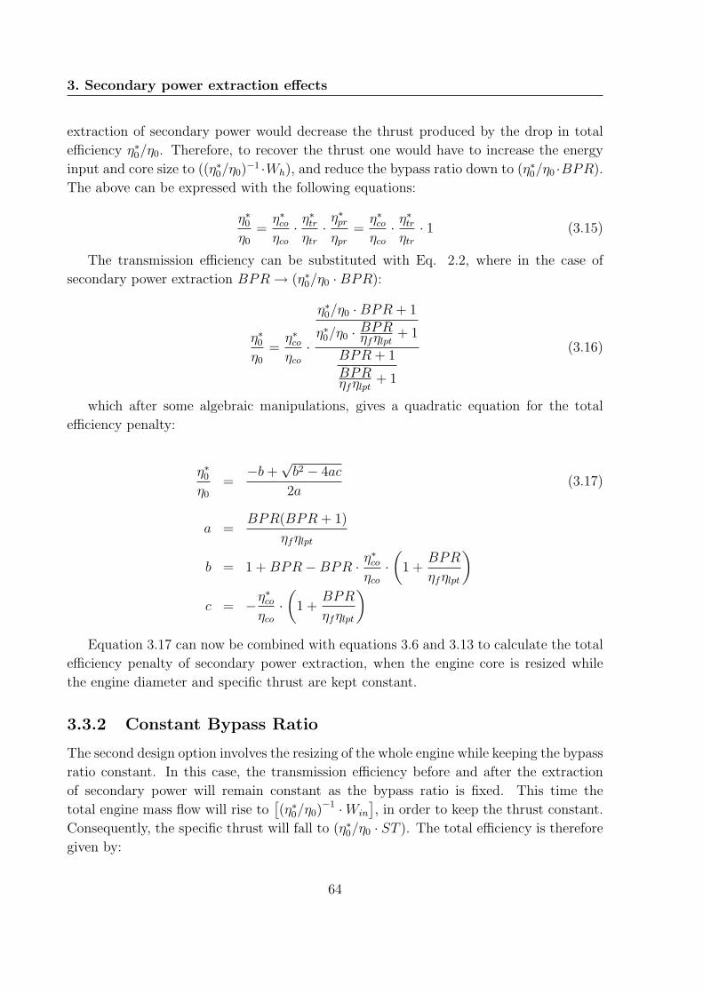
3. Secondary power extraction effects

extraction of secondary power would decrease the thrust produced by the drop in total

efficiency η∗0/η0. Therefore, to recover the thrust one would have to increase the energy

input and core size to ((η∗0/η0)−1 ·Wh), and reduce the bypass ratio down to (η∗0/η0 ·BPR).

The above can be expressed with the following equations:

η∗0η0

=η∗coηco· η∗tr

ηtr· η∗pr

ηpr=η∗coηco· η∗tr

ηtr· 1 (3.15)

The transmission efficiency can be substituted with Eq. 2.2, where in the case of

secondary power extraction BPR→ (η∗0/η0 ·BPR):

η∗0η0

=η∗coηco·

η∗0/η0 ·BPR + 1

η∗0/η0 · BPRηfηlpt + 1

BPR + 1BPRηfηlpt + 1

(3.16)

which after some algebraic manipulations, gives a quadratic equation for the total

efficiency penalty:

η∗0η0

=−b+

√b2 − 4ac

2a(3.17)

a =BPR(BPR + 1)

ηfηlpt

b = 1 +BPR−BPR · η∗co

ηco·(

1 +BPR

ηfηlpt

)c = −η

∗co

ηco·(

1 +BPR

ηfηlpt

)Equation 3.17 can now be combined with equations 3.6 and 3.13 to calculate the total

efficiency penalty of secondary power extraction, when the engine core is resized while

the engine diameter and specific thrust are kept constant.

3.3.2 Constant Bypass Ratio

The second design option involves the resizing of the whole engine while keeping the bypass

ratio constant. In this case, the transmission efficiency before and after the extraction

of secondary power will remain constant as the bypass ratio is fixed. This time the

total engine mass flow will rise to[(η∗0/η0)

−1 ·Win

], in order to keep the thrust constant.

Consequently, the specific thrust will fall to (η∗0/η0 · ST ). The total efficiency is therefore

given by:

64

3.4. Validation

Table 3.1: Engine specifications

Parameter Value Parameter Value

T [kN] 50 TET [K] 1200-2000

Mach 0.8 Alt [m] 10668

V0 [m/s] 237 ηf 0.9

OPR 40 ηlpt 0.86

BPR 2-50 ηhpt 0.88

Bypass ∆p/p [%] 1.5 ηhpc 0.86

Burner ∆p/p [%] 5.0 Ppo [kW] 0, 250, 500

∆hb [kJ/kg] 588 Wb [kg/s] 0, 0.425, 0.85

η∗0η0

=η∗coηco

η∗prηpr

=η∗coηco·

1

1 + η∗0/η0 · ST2V0

1

1 + ST2V0

(3.18)

which after some algebra gives:

η∗0η0

= − V0

ST+

V0

ST

√1 +

2ST

V0

η∗coηco

(1 +

ST

2V0

)(3.19)

3.4 Validation

The derived equations have been tested against numerical simulations for the engine spec-

ifications described in Table 3.1. The engine configuration resembles the one depicted in

Fig. 2.1, with a single-spool core which comprises a high-pressure compressor, a burner,

and a high-pressure turbine, followed by a low-pressure turbine driving a fan. The numer-

ical simulations have been conducted with Turbomatch. In a manner similar to [34], the

fan pressure ratio of each point on the graphs (representing a different engine) has been

optimised for minimum specific fuel consumption. At the same time the engine mass flow

has also been iterated in order to give a constant net thrust of 50 [kN].

Figures 3.2-3.5 compare the results of Eq. 3.6, 3.13, 3.17, and 3.19 with the simulation

results of Turbomatch for a TET = 1650 [K]. The SFC penalty shown in the figures is

calculated as[(η∗0/η0)

−1 − 1]· 100%. The results include shaft power and bleed air off-

takes and both the resizing methods described earlier. In all the cases the equations give

very good agreement with the simulation data for the whole range of bypass ratio. The

65

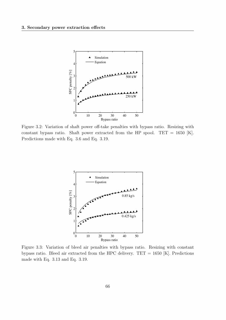
3. Secondary power extraction effects

0 10 20 30 40 500

1

2

3

4

5

Bypass ratio

SFC

pen

alty

[%]

SimulationEquation

500 kW

250 kW

Figure 3.2: Variation of shaft power off-take penalties with bypass ratio. Resizing with

constant bypass ratio. Shaft power extracted from the HP spool. TET = 1650 [K].

Predictions made with Eq. 3.6 and Eq. 3.19.

0 10 20 30 40 500

1

2

3

4

5

Bypass ratio

SFC

pen

alty

[%]

SimulationEquation

0.425 kg/s

0.85 kg/s

Figure 3.3: Variation of bleed air penalties with bypass ratio. Resizing with constant

bypass ratio. Bleed air extracted from the HPC delivery. TET = 1650 [K]. Predictions

made with Eq. 3.13 and Eq. 3.19.

66

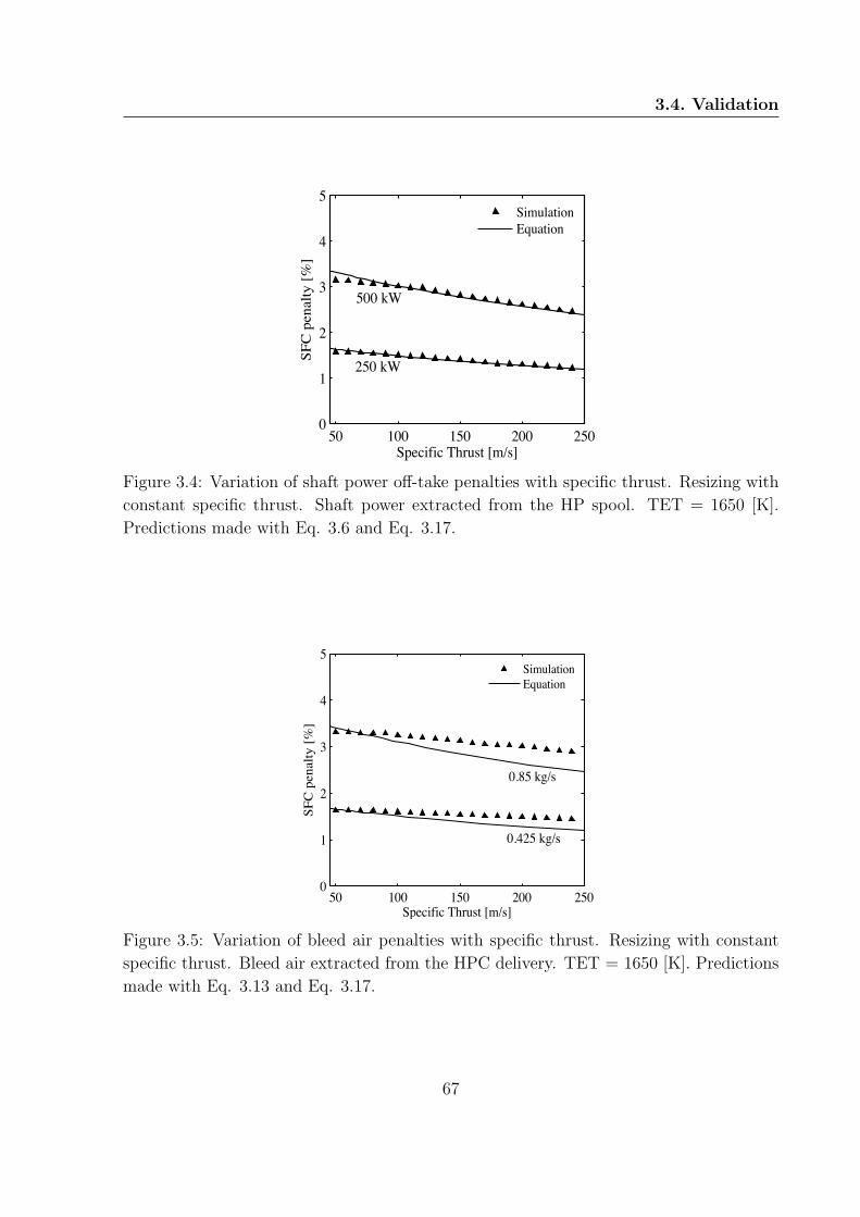
3.4. Validation

50 100 150 200 2500

1

2

3

4

5

Specific Thrust [m/s]

SFC

pen

alty

[%]

SimulationEquation

250 kW

500 kW

Figure 3.4: Variation of shaft power off-take penalties with specific thrust. Resizing with

constant specific thrust. Shaft power extracted from the HP spool. TET = 1650 [K].

Predictions made with Eq. 3.6 and Eq. 3.17.

50 100 150 200 2500

1

2

3

4

5

Specific Thrust [m/s]

SFC

pen

alty

[%]

SimulationEquation

0.85 kg/s

0.425 kg/s

Figure 3.5: Variation of bleed air penalties with specific thrust. Resizing with constant

specific thrust. Bleed air extracted from the HPC delivery. TET = 1650 [K]. Predictions

made with Eq. 3.13 and Eq. 3.17.

67

3. Secondary power extraction effects

1200 1400 1600 1800 2000

10

20

30

40

50

TET [K]

Byp

ass

ratio

0.4

0.2

0.2

0

0

0.2

0.2

0.2

0.4

0.4

Installed SFC prediction error [%]

Figure 3.6: Installed SFC prediction error throughout the whole range of BPR and TET.

Resizing with constant bypass ratio. 0.85 [kg/s] bleed air extracted from the HPC delivery.

The term installed SFC includes only the secondary power extraction penalty; no other

installation effect is included.

worst accuracy occurs in the case of the bleed air off-takes, where there is a deviation of

up to 17%. This, however, can be mainly attributed to the approximate determination

of the bleed enthalpy ∆hb, as Turbomatch returns the bleed temperature instead of the

enthalpy. It has to be underlined here that a penalty prediction error of 20% corresponds

approximately to an installed SFC prediction error of less than 0.5% (note here that the

term installed SFC does not include any other installation penalties apart from the ones

of secondary power extraction). For instance, if the real penalty is equal to 2% and the

predicted value is equal to 2.4% (i.e. 20% error), then the predicted installed SFC will be

(1.024 ∗ SFCbare) instead of (1.02 ∗ SFCbare). This translates to an installed SFC error

of (1.024 − 1.020)/1.020 ∗ 100% = 0.4%. Figure 3.6 shows the installed SFC prediction

error for the whole design space of bypass ratio and turbine entry temperature for the

worst-accuracy scenario of 0.85 kg/s bleed air. Even at the extremes of the design space

the error lies below 0.5%.

Therefore, Eq. 3.6 and 3.13 combined with Eq. 3.17 and 3.19 can be used to predict

the SFC penalty of shaft power and bleed air off-takes at the design point of the engine,

for engines that range from a turbojet to an open rotor.

68

3.5. Future Engines Penalties

3.5 Future Engines Penalties

The derived expressions are not only a useful tool for the determination of installed SFC

during the preliminary design phases but they also provide insight on how the extraction

of secondary power affects the performance of different engine designs. Whether future

engine designs such as ultra high bypass ratio engines or open rotors will face increasing

fuel consumption penalties is a question that can be approached using the developed

theory.

The first conclusion that can be drawn from the thermodynamic treatment of the

problem is the primary effect of secondary power on the core efficiency of the engine. Sec-

ondary power reduces the core efficiency, as the definition of core efficiency (Eq. 2.9) does

not include it as useful power output. Furthermore, Eq. 3.4 shows that for a given power

off-take the core efficiency penalty increases as the power produced by the core decreases.

The demand for core power does not come from the core per se, but from the demand for

a certain thrust. That is the reason why the propulsive and transmission efficiencies of the

engine dominate the magnitude of the penalty. For a given thrust requirement, the higher

the propulsive and transmission efficiencies, the lower the demand for core power as shown

by Eq. 3.5. Along these lines, the core efficiency and its drivers, i.e. the engine overall

pressure ratio and the turbine entry temperature, do not directly affect the penalty, but

they only have an indirect effect by defining the bypass ratio. More specifically, for a given

specific thrust the selection of overall pressure ratio and turbine entry temperature fixes

the value of bypass ratio, which in turn affects the transmission efficiency, and hence the

efficiency penalty. This finding comes to confirm Codner’s conclusions [74] about the lack

of relationship between the core characteristics and the secondary power SFC penalties.

Another way to justify the above is the following: by improving the core efficiency an

equal reduction in fuel needed is achieved for both the secondary and mainstream core

power, as they are both produced with the same efficiency; therefore the ratio between the

two, and thus the penalty, remains constant. The actual size of the core in terms of mass

flow has no effect either. For instance, if the TET and core specific power were increased,

the size of the core would decrease but the power produced by the core would remain

constant, as this is fixed by the thrust requirement and the propulsive and transmission

efficiencies. Therefore, the TET and actual size of the core would have no direct effect on

the penalty.

In addition to the primary effect on the core efficiency, the inclusion of secondary power

in the design point of the engine will also have a secondary effect either on the transmission

or the propulsive efficiency, depending on the resizing method employed. If the engine

is resized by keeping constant the specific thrust and diameter, while the core mass flow

is increased and the bypass ratio decreased, a transmission efficiency benefit will arise,

as shown by Eq. 2.2. On the other hand, if the engine is resized with constant bypass

69

3. Secondary power extraction effects

ratio and increased diameter, the specific thrust will fall and therefore the propulsive

efficiency will increase, as shown by Eq. 2.3. According to Peacock [4] it is this propulsive

efficiency gain that decreases the penalties for higher specific thrust engines. Following

this argument one could assume that if the engine was resized with constant specific thrust,

hence without any propulsive efficiency gain, the penalty would be constant for different

specific thrust engines. However, it has been shown in the thermodynamic analysis that

the propulsive efficiency gain is only a secondary effect, which is added on the primary

effect of the core efficiency drop. Even without any propulsive efficiency benefit the

penalty is higher for lower specific thrust engines as they have a smaller core and therefore

a higher core efficiency penalty (Fig. 3.4 and 3.5).

1200 1400 1600 1800 2000

100

200

300

400

TET [K]

Spec

ific

Thru

st [m

/s]

1.4

1.6

1.82

2.42.8

3.2

Bypass ratioSFC penalty [%]

375

15

10

Figure 3.7: SFC penalty prediction throughout the whole range of Specific Thrust and

TET. Resizing with constant bypass ratio. 500 [kW] of shaft power extracted from the

HP spool.

The variation of the penalty throughout the whole design space of TET and specific

thrust is shown in Fig. 3.7, for OPR = 40, resizing with constant bypass ratio, and

500 [kW] power extraction from the HP shaft. For a given TET as the specific thrust

decreases, the propulsive efficiency improves, the core power decreases and hence the

penalty increases. Similarly, for a given specific thrust as TET and hence bypass ratio

increases, the transmission efficiency falls, the core power increases and therefore the

penalty decreases. However, one can observe that this effect is weaker than the one of

specific thrust and it wanes completely after a bypass ratio of about 10, as after this point

the transmission efficiency decrease rate flattens out (Fig. 2.2).

Equations 3.6 and 3.13 reveal another cause of higher secondary power penalties for

future engines, also mentioned by Peacock [4]. More fuel-efficient aircraft/engine designs

70

3.5. Future Engines Penalties

will lead to lighter scaled-down aircraft with lower thrust requirements and, according to

Eq. 3.6 and 3.13, higher SFC penalties. Moreover, it is very likely that future engines

will face higher demands for secondary power due to the increased comfort offered to the

passengers. Equation 3.6 shows that the effects of the thrust and off-take power demand

can be combined into one non-dimensional power factor defined asPpoT · V0

. The power

factor can increase either by increasing the size of off-takes or by decreasing the required

thrust power.

0.1 0.3 0.5 0.7 0.9 1.1 1.3 1.5 1.70

1

2

3

4

5

6

7

0.010.03

0.050.07

0.09

P po

T · V 0

ST/V0

SFC

pena

lty [%

]

dfdlpt = 0.81

dfdlpt = 0.7

Figure 3.8: SFC penalty prediction of Eq. 3.19 and Eq. 3.6 for different specific thrusts

and non-dimensional power factors. Resizing with constant bypass ratio. Shaft power

extracted from the HP spool. BPR = 6.

Figure 3.8 shows the combined effect of the non-dimensional power factor and specific

thrust on the level of the penalties. The specific thrust has been non-dimensionalized

with the flight velocity. As shown earlier, bypass ratio has a lesser effect and can be

neglected, but the effect of transmission efficiency is still taken into account through

different fan and low-pressure turbine efficiencies. According to Fig. 3.8 lower specific

thrusts, higher fan and turbine efficiencies, and higher power factors lead to higher SFC

penalties. Furthermore, the higher the power factor, the more dependent is the penalty

on specific thrust. Figure 3.8 can be used as a map that approximately identifies the SFC

penalty for every engine and power off-take. It can also be used for the case of bleed air

off-takes ifWb∆hb1− β is used in the place of Ppo.

To conclude, it can be argued that future engines will suffer greater secondary power

SFC penalties due to:

71

3. Secondary power extraction effects

1200 1400 1600 1800 20000

50

100

150

200

250

TET [K]

Spec

ific

Thru

st [m

/s]

0.20.25

0.30.350.4

0.45

0.5

0.55

0.6pr benefit [%]

Figure 3.9: Propulsive efficiency gain when resizing with constant bypass ratio. 500 [kW]

of shaft power extracted from the HP spool.

1. Lower thrust requirements due to more efficient aircraft/engines.

2. Higher demand for secondary power.

3. Lower required core power for a given thrust, due to the more efficient conversion of

core power into thrust power achieved by engines with low specific thrust and high

fan and low-pressure turbine efficiencies.

However in absolute terms, the fuel needed for a given demand in secondary power will

remain constant unless improvements in core efficiency drive it down.

Altough the present study focuses on design point performance, a comment should

be made here with respect to the off-design performance of future engines. The higher

(secondary power)/(core power) ratio of future engines will also cause greater vertical

movements of the compressor running lines when the operating conditions or secondary

power requirements vary. This will affect the compressor surge margins and will also

cause a variation of component efficiencies. These effects should not be disregarded, but

a further off-design study is required in order to quantify them.

3.6 Resizing Methods Comparison

As described earlier, the two engine resizing methods only differ with respect to the

secondary effect of propulsive or transmission efficiency gains. This section investigates

72

3.6. Resizing Methods Comparison

the magnitude and variation of these gains, while it also compares the two methods in

terms of SFC.

1200 1400 1600 1800 2000

10

20

30

40

50

TET [K]

Byp

ass

ratio

0.02

0.04

0.060.080.10.12

tr benefit [%]

Figure 3.10: Transmission efficiency gain when resizing with constant specific thrust. 500

[kW] of shaft power extracted from the HP spool.

When the engine is resized with constant bypass ratio, the inlet mass flow increases and

a propulsive efficiency benefit accrues. As shown in Fig. 3.9, this benefit ranges from 0.6%

to 0.2% and decreases as the clean engine specific thrust falls. This happens because for

an increase in mass flow x, the decrease in specific thrust is ∆ST = ST (1− 1/x), which

decreases when ST falls resulting in a lower propulsive efficiency gain.

On the other hand, when the engine is resized by keeping a constant diameter and

allowing the core mass flow to increase and therefore the bypass ratio to decrease, a

transmission efficiency gain is attained. Figure 3.10 shows that this benefit is much lower

than the one achieved with the previous resizing method and depends only on bypass

ratio. The benefit decreases as the bypass ratio increases and diminishes after a bypass

ratio of 10. This behaviour is attributed to the steep variation of ηtr for low bypass ratios,

which flattens out after a bypass ratio of 10 (Fig. 2.2).

Figure 3.11 shows the SFC benefit of the constant BPR method relative to the constant

ST one. The relative benefit decreases: a) for lower STs following the trend shown in

Fig. 3.9; b) for BPRs lower than 10 according to Fig. 3.10. However, the constant

BPR method will result in a larger engine and consequently these small SFC benefits will

diminish as the weight and drag penalties come into play.

73

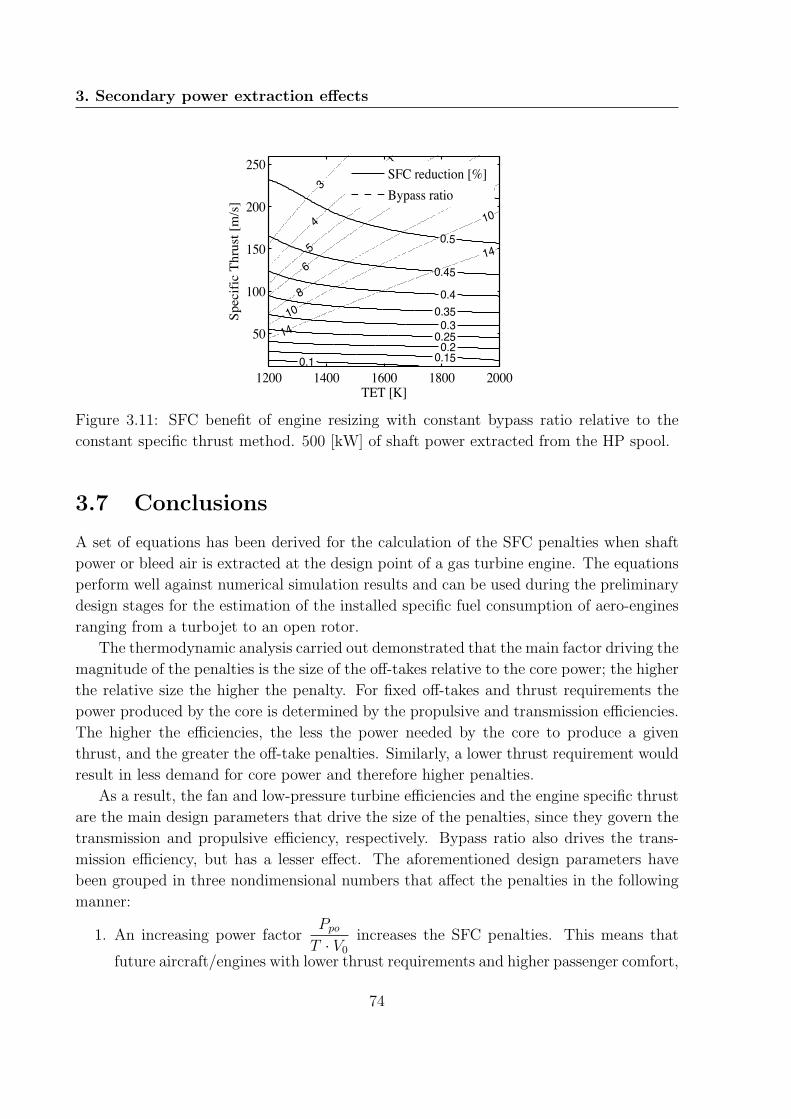
3. Secondary power extraction effects

1200 1400 1600 1800 2000

50

100

150

200

250

TET [K]

Spec

ific

Thru

st [m

/s]

0.1 0.150.20.250.30.350.4

0.45

0.5

0.543

4

56

8

8

10

10

14

14

SFC reduction [%]Bypass ratio

Figure 3.11: SFC benefit of engine resizing with constant bypass ratio relative to the

constant specific thrust method. 500 [kW] of shaft power extracted from the HP spool.

3.7 Conclusions

A set of equations has been derived for the calculation of the SFC penalties when shaft

power or bleed air is extracted at the design point of a gas turbine engine. The equations

perform well against numerical simulation results and can be used during the preliminary

design stages for the estimation of the installed specific fuel consumption of aero-engines

ranging from a turbojet to an open rotor.

The thermodynamic analysis carried out demonstrated that the main factor driving the

magnitude of the penalties is the size of the off-takes relative to the core power; the higher

the relative size the higher the penalty. For fixed off-takes and thrust requirements the

power produced by the core is determined by the propulsive and transmission efficiencies.

The higher the efficiencies, the less the power needed by the core to produce a given

thrust, and the greater the off-take penalties. Similarly, a lower thrust requirement would

result in less demand for core power and therefore higher penalties.

As a result, the fan and low-pressure turbine efficiencies and the engine specific thrust

are the main design parameters that drive the size of the penalties, since they govern the

transmission and propulsive efficiency, respectively. Bypass ratio also drives the trans-

mission efficiency, but has a lesser effect. The aforementioned design parameters have

been grouped in three nondimensional numbers that affect the penalties in the following

manner:

1. An increasing power factorPpoT · V0

increases the SFC penalties. This means that

future aircraft/engines with lower thrust requirements and higher passenger comfort,

74

3.7. Conclusions

and hence higher off-takes, will face increased SFC penalties.

2. Future engines are expected to have a decreased specific thrust factorST

V0

, which

will improve the propulsive efficiency, reduce the core power required for a given

thrust, and increase the off-take penalties.

3. An increasing transmission efficiency factor ηfηlpt reduces the core power required

for a given thrust and increases the off-take penalties.

The secondary-power SFC penalties are not high enough to affect the aforementioned

future trends; in other words, the benefits arising from reduced specific thrust and im-

proved transmission efficiency would outweigh the increased secondary-power penalties.

Reducing the power factor appears to be the only way to improve the situation for future

engines. This could be achieved by designing more efficient secondary systems, possibly

within the context of an all-electric aircraft. The characteristics of the core (TET, OPR,

core component efficiencies and pressure losses) do not directly affect the relative penal-

ties, although they influence the absolute fuel needed for the provision of secondary power.

In light of this, improvements in core efficiency should be further pursued to reduce the

fuel burned for secondary systems and primary propulsive power.

When redesigning an engine to include the secondary power extraction in the design

point, two methods exist to conduct the resizing:

1. Resize the whole engine by keeping the bypass ratio constant.

2. Resize the core by keeping the diameter and specific thrust constant.

Each method has a different secondary effect on the size of the penalties. The first

method results in a propulsive efficiency benefit, accruing from the higher mass flow and

lower specific thrust of the resized engine. The second method results in a lesser transmis-

sion efficiency benefit due to the lower bypass ratio of the resized engine. Although, the

first method results in a better SFC the higher size of the engine is expected to increase

its weight and drag and therefore eliminate or even reverse the fuel consumption benefit.

75

3. Secondary power extraction effects

76

Chapter 4

Propeller modelling method

development

4.1 Introduction

This chapter aims to develop a propeller performance modelling methodology suitable

for the study of high speed prop-fans. This model constitutes the first step towards the

implementation of an open-rotor simulation capability of equal maturity to the simulation

of turbofans. The created tool will be used in the next chapter in order to devise a

propeller map scaling technique, required for the integrated open-rotor engine performance

prediction.

The chapter starts by identifying the main parameters that govern the propeller per-

formance with a detailed analysis of the different sources of losses. This is followed by

an extensive review of the different modelling approaches, leading to the selection of the

lifting-line theory appropriately adapted for the simulation of advanced high speed prop-

fan blades. The next sections detail the step by step development of the model, while

special emphasis is given to the treatment of compressibility effects and the modelling

of the propeller wake. The validity of the method is tested against experimental data

and another higher fidelity numerical approach. The test case used for the validation is a

swept prop-fan geometry designed by NASA and Hamilton Standard in the ’70s.

4.2 Propeller fundamentals

The non-dimensional parameters most commonly used for the definition of propeller per-

formance are the power coefficient CP , the advance ratio J , the flight Mach number M0,

the thrust coefficient CT , and the propeller efficiency ηprop, the last two being traditionally

the dependent variables [78]. The operating Reynolds number also affects the propeller

77

4. Propeller modelling method development

performance but its effect is usually considered secondary and it is not taken into account

[79]. This is a good assumption if the the Reynolds number at the 0.75 radius is higher

than 7× 105, which is the case most of the times for full-scale propellers. The power and

thrust coefficients are simply the non-dimensional forms of the power used and the thrust

generated by the propeller and are defined according to Eq. 4.1 and Eq. 4.2 respectively.

As shown by Eq. 4.3, the advance ratio is defined as the distance the propeller covers in

one revolution divided by the propeller diameter. The propeller efficiency is defined as

the ratio of thrust power upon input power and can be calculated by Eq. 4.4. Finally, a

last parameter commonly used is the propeller disk loading, which - as shown by Eq. 4.5 -

is defined as the ratio of the power input divided by the square of the propeller diameter.

The disk loading is analogous to the fan pressure ratio of turbofan engines [80] and it

shows the amount of kinetic energy imparted to the air as it passes through the propeller

disk.

CP =P

ρ · n3 ·D5(4.1)

CT =T

ρ · n2 ·D4(4.2)

J =V0

n ·D (4.3)

ηprop =T · V0

P=CT · JCP

(4.4)

P/D2 =CPJ3· ρ · V0

2 (4.5)

Propeller maps are usually presented as contour plots of efficiency as a function of

CP and J . For each different Mach number a different contour plot is required. For the

benefit of easier digitization and numerical interpolation, sometimes efficiency is replaced

by CT [81].

It is useful at this point to make some comments on the losses impacting the propeller

efficiency. An understanding of the losses breakdown will set the basis and the require-

ments for the selection of a propeller analysis method. For a propeller that measures 80%

of efficiency, the 20% of losses can be broken down as follows. The axial and swirl momen-

tum imparted to the air as it passes through the propeller disk represent approximately

3 and 7 percent units [82]. These momentum losses are higher the higher the loading

of the propeller. As a notion these losses can be related to the propulsive efficiency of

a jet engine, where the losses increase for higher jet velocities. For a finite number of

blades there is also a 5% ”tip-loss” connected to the reduction of lift near the blade edges,

due to the presence of the tip vortices and the propeller wake [80]. This phenomenon

78

4.3. Analysis methods

corresponds to the induced drag of finite wings, and is aggravated as the loading increases

(due to stronger vortices) and as the number of blades decreases. All the aforementioned

losses, which so far account for 15% out of the 20% of total losses, are ideal losses [83].

This means that they are present even at the ideal condition of zero drag and hence zero

viscous losses. Finally, viscous losses account for 5% of the total and can exceed the value

of 7% as the Mach number increases [80]. This loss breakdown shows the importance of

accurately modelling the ideal performance of the propeller, which must then be coupled

with a reliable source of airfoil drag polars to account for the viscous losses.

4.3 Analysis methods

Wald [84] gives a very concise account of the historical evolution of propeller analysis

methods. The beginning was made with the axial momentum theory by Rankine [85] and

Froude [86], which, albeit their simplicity, only account for the axial momentum losses.

Furthermore, these methods do not take into account the actual blade geometry since

they model the propeller as an actuator disk. According to the propeller loss analysis

presented in the previous section, these methods can only represent 3 percent units of

the total losses. The Axial Momentum theory was extended by the General Momentum

theory that is also capable of calculating the swirl induced velocity component [87–89].

A different path was followed by Drzewiecki, who developed the first blade-element

theory [90]. This theory is the base of almost every modern preliminary propeller analysis

method [79]. The fundamental assumption of this theory is that the blade is discretised in

2D ”strips” or ”blade elements” whose performance is independent of one another. The

angle of attack of each blade element can be calculated by knowing the free-stream velocity

components, which result from the axial flight velocity and the rotational propeller speed.

This angle of attack is then used as an input to a 2D airfoil database to read the blade

element lift and drag coefficients, and calculate the lift and drag forces. The integration

of these forces along the blade will yield the total propeller performance. This method

accounts for the actual blade geometry and is able to calculate the viscous drag losses.

However, the viscous losses contribute only 5-7 percent units to the total losses figure.

The prediction of such methods falls far from the truth, as in reality the blade elements

are not independent [91]. Hence, the blade-element model needs to be coupled to another

theory that is capable of calculating the induced velocities.

The Wright brothers are deemed as the first who coupled the two aforementioned

modelling approaches and created the combined Blade-Element Momentum theory (BEM)

[84], which was then described in detail by Glauert [89]. This method is able to describe

the sum of momentum losses and viscous drag losses that amount to 15-17 percent units

of the total losses. With the addition of the Prandtl tip loss function [89, 92], this method

has survived until today due to its simplicity and its fairly good results [84, 87, 93, 94].

79

4. Propeller modelling method development

Nonetheless, albeit the correction introduced by the Prandtl tip loss function, the BEM

method still assumes an averaged wake flow and is not able to accurately model the effect

of the exact propeller wake. Furthermore, the method is not capable to calculate the

velocity outside the defined flow stream-tube, or simulate the time-dependent performance

of the rotor [95]. These shortcomings could limit future extension of the method to the

field of noise estimation.

As described earlier, similarly to wings, there is a sheet of trailing vorticity shed in the

wake of the blade, with the strongest vortices being at the tip of the blade [96]. Betz was

the first to prove that for lightly-loaded optimum propellers the wake assumes the form of

a rigid helical surface [92]. Prandtl calculated the induced velocity field produced by such

a wake by approximating the wake by a set of equally spaced semi-infinite lamina and

produced what is known as the Prandtl Tip Loss function [92]. The first exact algebraic

solution to the wake defined by Betz was given by Goldstein in 1929 [97], who solved

the potential flow equation problem by using Bessel functions. Theodorsen extended the

applicability of the method to high loadings but used an electrical analogy of the helical

wake, and a set of experiments to calculate the induced velocities [98]. These methods

have been widely used until today for the design and performance prediction of straight

blade single [84, 99–106] and contra-rotating propellers [22, 23, 107–109].

The advent of high-speed prop-fans which feature highly swept blades brought to the

surface the main limitation of the Goldstein methods. For the case of straight blades one

needs only to consider the effect of the trailing wake vorticity on the induced velocity, as

the vorticity ”bound” to the straight blades induces no velocity [84, 110]. However that

is not the case for swept blades, as it will be shown in the next sections when the method

development will be described. Hamilton Standard, the company who designed the SR

prop-fan family in the ’70s, identified that problem after designing the SR1 and SR2

propellers using a Goldstein method [80, 82, 103]. The modelling efforts by NASA [111–

114] and ONERA [115] led to the same conclusion regarding the unsuitability of Goldstein

based methods for the simulation of swept blades. Both NASA [114] and ONERA [115]

found that neglecting the effect of bound vorticity displaces inboard the maximum loading

of the blade.

Hamilton standard decided to design the rest of the SR family propellers by using the

curved lifting-line method [100, 101, 105, 116] and the same approach was followed by

NASA [117, 118] and by ONERA [115, 119–121]. This method is regarded as the extension

of Prandtl’s lifting-line wing method [122] to the case of swept propeller blades. According

to its fundamental principle the blade is replaced by a curved vortex filament which

passes through the quarter chord point of every section. As the circulation varies from

one blade element to the next, trailing vortices spring from the blade-element boundaries

according to the vortex theorems stated by Helmholtz [96]. These trailing vortices follow

approximately a helical trajectory, which can be prescribed [123] or calculated freely

80

4.4. Lifting-line method development

[124, 125]. The influence of the bound and trailing vortices on the blade is calculated by

using the law of Biot-Savart [126, 127]. The approach is therefore capable of handling

correctly the effect of bound and trailing vorticity, while taking into account a more

realistic wake geometry.

Despite the development of more advanced lifting-surface, Euler and CFD techniques,

the lifting-line approach is still used today during the propeller preliminary design stages,

and in order to predict the propeller global performance [121, 128]. Furthermore, higher

complexity methods do not always give higher fidelity results, an argument confirmed

by Burger [129], who compared a lifting-surface and a lifting-line method. As this work

focuses on the global performance of propellers, which represents a brick in the whole

engine performance prediction, the lifting-line method has been chosen. This choice is also

based on the experience gained by working with the Goldstein and Theodorsen methods

within the MSc theses of Iosifidis [130] and Sanchez-Ortega [131], which confirmed the

aforementioned shortcomings of these approaches. The details of the developed lifting-

line approach will be presented in the next sections, while the validation of the method

against experimental data and higher order methods will prove that not much accuracy

has been sacrificed.

4.4 Lifting-line method development

4.4.1 Coordinate systems

Before presenting the details of the method it is crucial to first lay the foundations by

discussing the coordinate systems used for the analysis. Figure 4.1 presents the global

coordinate systems used. The first system is a cartesian XYZ orthogonal system that is

fixed on the base of the pitch change mechanism and rotates with the propeller. This

choice has been made instead of an inertial system, as in this way the unsteady flow

problem is converted to a steady one. In this work the Z-axis, which is the axis of rotation,

is also parallel to the direction of flight as no angle of attack is considered. The X-axis

is aligned to the pitch change mechanism that passes through the middle of the base of

the blade and together with the Y-axis define the plane of rotation. The cartesian XYZ

system is used for the input of the geometry and also as the common base of reference

for the calculations. The corresponding cylindrical rφZ system is used when needed to

facilitate the calculations by exploiting the symmetry of the geometry.

Apart from these global coordinate systems, another local one is defined at each blade

element. As shown in Figs. 4.1 and 4.2 the s-axis is tangent to the meanline of the blade

and points from the hub to the tip. The c-axis is parallel to the chord, perpendicular

to the s-axis and points from the trailing edge to the leading edge of the airfoil. Finally

the n-axis is normal to the other two and is a result of their cross product. The local

81

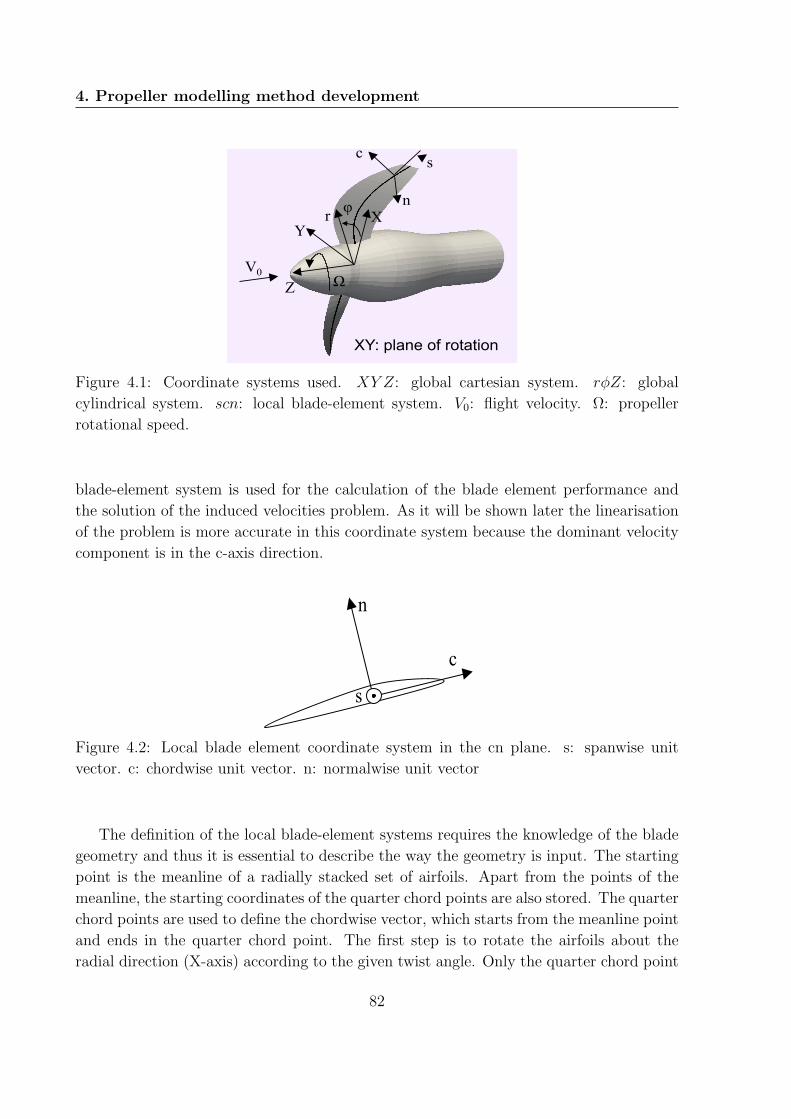
4. Propeller modelling method development

X

Z

Y

n

s c

Ω V0

XY: plane of rotation

r φ

Figure 4.1: Coordinate systems used. XY Z: global cartesian system. rφZ: global

cylindrical system. scn: local blade-element system. V0: flight velocity. Ω: propeller

rotational speed.

blade-element system is used for the calculation of the blade element performance and

the solution of the induced velocities problem. As it will be shown later the linearisation

of the problem is more accurate in this coordinate system because the dominant velocity

component is in the c-axis direction.

c

n

s

Figure 4.2: Local blade element coordinate system in the cn plane. s: spanwise unit

vector. c: chordwise unit vector. n: normalwise unit vector

The definition of the local blade-element systems requires the knowledge of the blade

geometry and thus it is essential to describe the way the geometry is input. The starting

point is the meanline of a radially stacked set of airfoils. Apart from the points of the

meanline, the starting coordinates of the quarter chord points are also stored. The quarter

chord points are used to define the chordwise vector, which starts from the meanline point

and ends in the quarter chord point. The first step is to rotate the airfoils about the

radial direction (X-axis) according to the given twist angle. Only the quarter chord point

82

4.4. Lifting-line method development

coordinates are affected by this rotation as the meanline coincides with the rotation axis.

The next step is to sweep back along the extended chord line. This geometry definition

method is equivalent to the one used by Hamilton Standard for the design of the SR1

propeller [104]. The final step is to rotate the blade along the pitch change mechanism

axis by the desired pitch angle. In this starting position the coordinates of the meanline

and quarter chord line are known in the XYZ system. This geometry definition method

can be used if the geometry is given as a table of chord, twist and sweep angle. If the

exact 3D geometry is known, the exact XYZ coordinates of the meanline and quarter

chord points can be given.

By knowing the coordinates of the meanline and quarter chord points for each blade

station, the local blade-element unit vectors can be defined as follows. The spanwise unit

vector is the difference between two adjacent meanline points (outboard minus inboard).

The chordwise unit vector, as mentioned earlier, is the difference between the quarter

chord point and the meanline point. The normalwise unit vector is the product vector of

the two others and should point from the pressure side to the suction side of the airfoil.

All the vectors should be divided by the scalar value of their magnitude to ensure that

they have unit length. Their magnitude is defined as the square root of the sum of squares

of the unit components. The above definitions are reflected on the Eqs. 4.6-4.8, which

define the unit vectors for the center of each blade element i.

~es,(i) =αsX ,(i)d· ~eX +

αsY ,(i)d· ~eY +

αsZ ,(i)d· ~eZ (4.6)

αsX ,(i) = Xm,(i+1) −Xm,(i)

αsY ,(i) = Ym,(i+1) − Ym,(i)αsZ ,(i) = Zm,(i+1) − Zm,(i)

d =√α2sX ,(i)

+ α2sY ,(i)

+ α2sZ ,(i)

~ec,(i) =αcX ,(i)d· ~eX +

αcY ,(i)d· ~eY +

αcZ ,(i)d· ~eZ (4.7)

αcX ,(i) = X1/4c,(i) −Xm,(i)

αcY ,(i) = Y1/4c,(i) − Ym,(i)αcZ ,(i) = Z1/4c,(i) − Zm,(i)

d =√α2cX ,(i)

+ α2cY ,(i)

+ α2cZ ,(i)

83

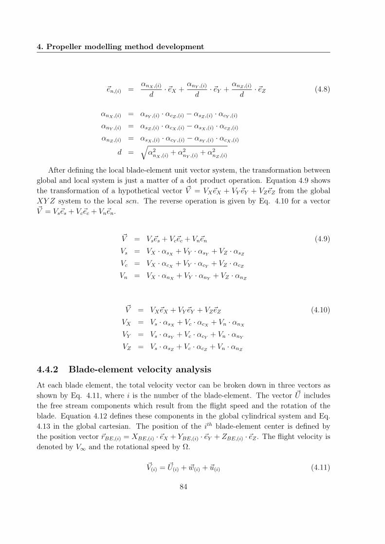
4. Propeller modelling method development

~en,(i) =αnX ,(i)d· ~eX +

αnY ,(i)d· ~eY +

αnZ ,(i)d· ~eZ (4.8)

αnX ,(i) = αsY ,(i) · αcZ ,(i) − αsZ ,(i) · αcY ,(i)αnY ,(i) = αsZ ,(i) · αcX ,(i) − αsX ,(i) · αcZ ,(i)αnZ ,(i) = αsX ,(i) · αcY ,(i) − αsY ,(i) · αcX ,(i)

d =√α2nX ,(i)

+ α2nY ,(i)

+ α2nZ ,(i)

After defining the local blade-element unit vector system, the transformation between

global and local system is just a matter of a dot product operation. Equation 4.9 shows

the transformation of a hypothetical vector ~V = VX~eX + VY ~eY + VZ~eZ from the global

XY Z system to the local scn. The reverse operation is given by Eq. 4.10 for a vector~V = Vs~es + Vc~ec + Vn~en.

~V = Vs~es + Vc~ec + Vn~en (4.9)

Vs = VX · αsX + VY · αsY + VZ · αsZVc = VX · αcX + VY · αcY + VZ · αcZVn = VX · αnX + VY · αnY + VZ · αnZ

~V = VX~eX + VY ~eY + VZ~eZ (4.10)

VX = Vs · αsX + Vc · αcX + Vn · αnXVY = Vs · αsY + Vc · αcY + Vn · αnYVZ = Vs · αsZ + Vc · αcZ + Vn · αnZ

4.4.2 Blade-element velocity analysis

At each blade element, the total velocity vector can be broken down in three vectors as

shown by Eq. 4.11, where i is the number of the blade-element. The vector ~U includes

the free stream components which result from the flight speed and the rotation of the

blade. Equation 4.12 defines these components in the global cylindrical system and Eq.

4.13 in the global cartesian. The position of the ith blade-element center is defined by

the position vector ~rBE,(i) = XBE,(i) · ~eX + YBE,(i) · ~eY + ZBE,(i) · ~eZ . The flight velocity is

denoted by V∞ and the rotational speed by Ω.

~V(i) = ~U(i) + ~w(i) + ~u(i) (4.11)

84

4.4. Lifting-line method development

~U(i) =(−Ω ·

√X2BE,(i) + Y 2

BE,(i)

)· ~eφ + (−V∞) · ~eZ (4.12)

~U(i) =(Ω · YBE,(i)

)· ~eX +

(−Ω ·XBE,(i)

)· ~eY + (−V∞) · ~eZ (4.13)

The vector ~u describes the velocity components induced by the presence of a spinner

and a nacelle. This velocity variation can be calculated by using a panel method which

solves the potential flow equation [132] for a given spinner/nacelle geometry. Panel meth-

ods are extensively used in the industry as routine design tools for three-dimensional flows

[133]. This work uses the publicly available code Panair, developed by Boeing, which has

been extensively tested and validated in several cases for subsonic and supersonic flows

[133]. A similar approach has been followed by Mikkelson et al [82] for the modelling

of the SR1 and SR2 prop-fans. The schematic in Fig. 4.3 shows the way the code is

used for the purposes of this work. The code requires the input of the flow velocity, the

coordinates of the grid points that represent the nacelle geometry and the coordinates

of the off-body points where the induced velocity needs to be calculated. The output

includes the velocity vector ~u components at each off-body point which can then be used

as an input in the lifting line method. For this work the off-body points of interest are

the lifting-line points which are located at the quarter chord line of the blade.

¼ chord line (x,y,z)

0,1 0,3 0,5 0,7 0,9 1,1 -10

0

10

20

30

40

50

r/R

u [m

/s]

ux uy uz

PANAIR input

X

Z Y

V0

PANAIR

Body grid (x,y,z)

Figure 4.3: Panair input and output data.

The last vector ~w is the velocity induced by the trailing vortices of the wake and

the bound vortices of the blades on each point of the blade. For simplicity henceforth

it will be called vortex induced velocity. This induced velocity depends on the geometry

of the wake, the geometry of the blades and on the operating conditions. Its calculation

is the topic of the following sections. It has to be underlined here that in reality the

nacelle induced and the vortex induced velocities interact with each other; i.e. the two

85

4. Propeller modelling method development

calculations should be coupled in an iterative process. However for prop-fan applications

this coupling is commonly omitted without a significant loss in accuracy [117].

4.4.3 Wake geometry definition

As mentioned in the literature review presented in section 4.3, the lifting line theory

hypothesizes the existence of two types of vortices. Bound vortices that pass through

the quarter chord line of the blades and corresponding trailing vortices that spring from

the blade-element boundaries and constitute the wake of the propeller (Fig. 4.4). It is

essential for the set-up and solution of the problem that a decision is made regarding the

wake geometry. There are three main approaches:

1. The rigid wake which has been followed by Goldstein [97]. According to this method

the wake assumes the shape of a rigid screw surface which follows a constant helix

angle at every radius. This assumption neglects the influence of the induced velocity

in the wake and can lead to significant inaccuracies at high loading conditions [113].

Furthermore, the wake is assumed to be non-contracted, i.e. there is no change in

the radial position of the trailing vortices. This can again lead to inaccuracies when

a static performance prediction is sought. The advantages of the method lies in the

fact that the wake is defined a priori and remains constant throughout the entire

iteration process [87].

2. The prescribed wake method. This method allows each helix to have a different

angle by taking into account the local induced velocity [119]. It can also take into

account the contraction by applying a set of correlations derived from experimental

data [123], most notably the ones produced by Landgrebe [117, 123]. After the

vortex is shed the helix angle remains constant [134]. It is evident that in this case

the wake must be updated in each iteration as it is affected by the current value of

the induced velocities. According to Young, 2-3 iteration are enough for the wake

to assume its final shape [123].

3. The free wake method. This technique does not prescribe the wake geometry but it

allows its real time calculation [124, 125]. It requires a much higher computational

time than the other two methods and it is commonly used to calculate the static

performance of propellers, where the contraction is significant. Alternatively it can

be used to calibrate a prescribed wake model. At normal speed conditions it does

not offer a higher accuracy advantage relative to the prescribed wake method as

reported by Gur and Rosen [87].

This work focuses on the propeller global performance prediction for Mach greater

than 0.2 which is a typical end-of-runway speed. The details of the wake geometry and

86

4.4. Lifting-line method development

Bound vortex line at ¼ chord

Trailing vortex filaments springing from the bound vortex segment

boundaries

Figure 4.4: The modelling of the blade with a bound vortex and of the wake with a set

of trailing vortex filaments.

the more complicated and resource demanding static performance prediction are outside

the scope of work and therefore the selection of a free-wake model is not justified. The

author has selected the prescribed wake formulation as presented by Egolf et al [117] for

a similar prop-fan application. According to this model the local helix angle of the ith

filament is calculated by Eq. 4.14 where only the axial induced velocity is taken into

account. Furthermore the speeds under which a prop-fan normally operates allow the

omission of the wake contraction without a significant loss of accuracy. This is a common

assumption used widely in the literature [118, 119, 134]. Nevertheless, the selection of

a prescribed wake approach allows for future implementations of contraction prediction

correlations, similar to Refs. [117] and [123].

tan(φh,(i)) =V∞ + wZ,(i)

Ω ·√X2W,(i) + Y 2

W,(i)

(4.14)

Each vortex filament is segmented into straight vortices according to the geometric law

described by Eq. 4.15. Equation 4.15 is a simple geometric series that gives the azimuthal

angle of each vortex filament point in the cylindrical system. Two points define a straight

segment.

φaz,(j) = NWT · 2π ·(

j − 1

NWP − 1

)gw(4.15)

In Eq. 4.15 NWT is the number of turns a wake vortex filament is allowed to develop

for, NWP the number of points the vortex filament is split into and j = 1..NWP the current

filament point. Normally 4 wake turns are sufficient, while the number of wake points

has to be adjusted to give less than 2.5 for the first segment [127]. The parameter gw

87

4. Propeller modelling method development

controls the grading of the grid and can take a value around 1.6. This way the first vortex

segments that have the greatest impact on the performance calculations will be smaller

than the vortex segments further from the blade.

The radius of each filament is kept constant and equal to the radius of the point on the

bound vortex where the trailing filament springs from. The last coordinate to be defined

is the Z which is given by Eq. 4.16 for the point j of the filament i. Equation 4.16 is

consistent with the helix angle definition of Eq. 4.14. The result of this wake definition

is shown in Fig. 4.5.

ZW,(i,j) =φaz,(j)

Ω·(V∞ + wZ,(i)

)(4.16)

Figure 4.5: The resulting non-contracted prescribed wake geometry.

It is evident from Eq. 4.16 that the wake geometry depends on the variation of induced

velocity along the blade radius. However this velocity is not known when the calculation

begins and stems from the wake geometry itself. It is for this reason that the calculation

requires a number of iterations, where for each calculation of induced velocities the wake

geometry is updated. For the initial definition of the wake the induced velocities can be

assumed to be zero, and hence the wake starts as a rigid helix surface.

4.4.4 Biot-Savart law

After the position of the bound and trailing vortices is defined, their influence can be

calculated by using the law of Biot-Savart [127]. This law gives the velocity ~w induced at

a point P by a vortex segment ~lAB that has a constant circulation of Γ, as shown by Fig.

4.6 for a straight vortex segment.

~w =Γ

4π

h

(r2nc + h2n)1/n

(cos θ1 − cos θ2)~lAB × ~r1|~lAB × ~r1|

(4.17)

~r1 = ~rP − ~rA, ~r2 = ~rP − ~rB, ~lAB = ~rB − ~rA (4.18)

88

4.4. Lifting-line method development

Γ

B

A

P

wx

wy

wz

θ1

θ2

h

r1

r2

Vortex core

Figure 4.6: The Biot-Savart law, giving the velocity ~w induced by a straight vortex

segment ~lAB with a finite core radius as given by Leishman [127].

h = r1sinθ1 = r2sinθ2 (4.19)

cos θ1 =~lAB · ~r1|~lAB| · |~r1|

, cos θ2 =~lAB · ~r2|~lAB| · |~r2|

(4.20)

where rp, rA and rB are the position vectors of the points P, A and B in the global XY Z

system.

After all the wake segments are defined as described in the previous sections, the set

of equations 4.17-4.20 can be used to find the velocity induced by each segment of bound

and trailing vorticity. Some remarks should be made about the use of a ”vortex core” in

Eq. 4.17. If the Biot-Savart law is used without a vortex core (rc = 0) Eq. 4.17 results in

an infinite induced velocity when h → 0. This behaviour of the Biot-Savart law results

from its irrotational flow nature which is unrealistic as we move closer to the vortex core.

Leishman [127] describes the salient points of different vortex core models and Eq. 4.17,

which is taken from there, uses the Vatistas model. The parameter n in Eq. 4.17 defines

the velocity profile in the vortex core according to the Vatistas method. In the context

of this work the vortex core modelling is only a tool of de-singularisation and a more

detailed treatment of vortex dynamics falls outside the scope of work. Szymendera [135]

reports that different vortex core modelling choices have negligible effect on the global

performance and therefore the author made the choice of n = 2 without any further

investigation. The vortex core radius rc is calculated using the Lamb-Oseen model as

described by Ananthan et al [136].

Finally, an important observation can be made for Eq. 4.17. The induced velocity is

equal to the product of the circulation of the vortex segment Γ with a vector geometric

89

4. Propeller modelling method development

coefficient ~GC, which is only a function of the geometry of the segment that in turn stems

from the geometry of the wake. Therefore Eq. 4.17 can be conveniently rearranged to

give Eq. 4.21.

~w = Γ · ~GC (4.21)

4.4.5 Vortex induced velocity calculation

The calculation of the vortex induced velocity at any blade element of the lifting line can

be conducted, starting from the simple Eq. 4.21. At this point the segmentation of the

blade and wake must be recapitulated with the help of Fig. 4.7. Each one of the NB blades

is modelled as a bound vortex that is split into N blade elements. These elements have

constant circulation and are bounded by N + 1 points. From these points spring N + 1

trailing vortex filaments that are split into NWP − 1 straight vortex segments (according

to the discretisation of the wake as given by Eq. 4.15). The circulation is constant along

the length of a trailing vortex filament and is equal to the circulation difference between

the two bound vortex segments adjacent to the origin of the filament (Fig. 4.8).

1

2

N

…

1 2 … NWP-1

…

…

…

Bla

de e

lem

ents

i =

1 ...

N

Trai

ling

vorte

x fil

amen

ts k

= 1

... N

+1

1

2

…

N+1

Filament segments j = 1 ... NWP-1

…

…

…

…

Figure 4.7: The discretisation of the blade and the wake. The blade is depicted with grey

background.

The first step is the calculation of the velocity induced by the trailing vorticity. The

velocity induced on the ith blade element, by the jth segment, of the kth trailing filament,

of the lth blade is:

90

4.4. Lifting-line method development

Leading edge Γi-1 Γi Γi+1

Γi-1- Γi Γi- Γi+1

Bound vortex segment

Trailing filament

Trailing edge

Figure 4.8: The relation between bound and trailing vortex circulation.

~wTR,(i,j,k,l) = ΓTR,(k) · ~GCTR,(i,j,k,l) (4.22)

where ΓTR is the circulation of the trailing filament. Then the total induced velocity from

the kth trailing filament of all the blades is:

~wTR,(i,k) = ΓTR,(k) ·NB∑l=1

NWP−1∑j=1

~GCTR,(i,j,k,l) = ΓTR,(k) · ~GCTR,(i,k) (4.23)

Therefore the velocity induced by all the trailing vortex filaments is given by:

~wTR,(i) =N+1∑k=1

ΓTR,(k) · ~GCTR,(i,k) (4.24)

From Fig. 4.8 the trailing circulation of the kth filament can be defined as ΓTR,(k) =

Γ(k−1)−Γ(k), where Γ(k) is the circulation of the i = k blade element. In the special cases

where k = 1 or k = N + 1⇒ Γ(k) = 0. Hence Eq. 4.24 can be rewritten as:

~wTR,(i) =N+1∑k=1

(Γ(k−1) − Γ(k)

)· ~GCTR,(i,k) (4.25)

which can then be regrouped in terms of Γ(k) to give:

~wTR,(i) =N∑k=1

Γ(k) ·[~GCTR,(i,k+1) − ~GCTR,(i,k)

]=

N∑k=1

Γ(k) · ~GC∗TR,(i,k) (4.26)

91

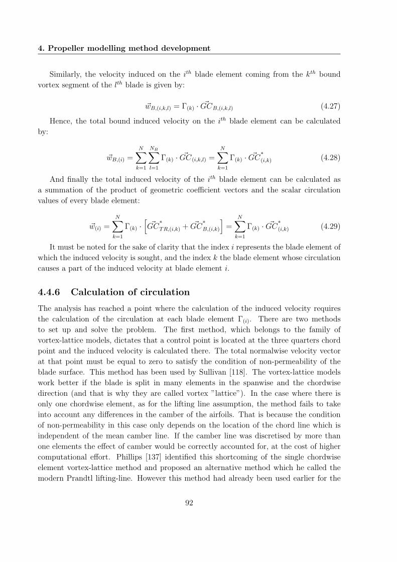
4. Propeller modelling method development

Similarly, the velocity induced on the ith blade element coming from the kth bound

vortex segment of the lth blade is given by:

~wB,(i,k,l) = Γ(k) · ~GCB,(i,k,l) (4.27)

Hence, the total bound induced velocity on the ith blade element can be calculated

by:

~wB,(i) =N∑k=1

NB∑l=1

Γ(k) · ~GC(i,k,l) =N∑k=1

Γ(k) · ~GC∗(i,k) (4.28)

And finally the total induced velocity of the ith blade element can be calculated as

a summation of the product of geometric coefficient vectors and the scalar circulation

values of every blade element:

~w(i) =N∑k=1

Γ(k) ·[~GC∗TR,(i,k) + ~GC

∗B,(i,k)

]=

N∑k=1

Γ(k) · ~GC∗(i,k) (4.29)

It must be noted for the sake of clarity that the index i represents the blade element of

which the induced velocity is sought, and the index k the blade element whose circulation

causes a part of the induced velocity at blade element i.

4.4.6 Calculation of circulation

The analysis has reached a point where the calculation of the induced velocity requires

the calculation of the circulation at each blade element Γ(i). There are two methods

to set up and solve the problem. The first method, which belongs to the family of

vortex-lattice models, dictates that a control point is located at the three quarters chord

point and the induced velocity is calculated there. The total normalwise velocity vector

at that point must be equal to zero to satisfy the condition of non-permeability of the

blade surface. This method has been used by Sullivan [118]. The vortex-lattice models

work better if the blade is split in many elements in the spanwise and the chordwise

direction (and that is why they are called vortex ”lattice”). In the case where there is

only one chordwise element, as for the lifting line assumption, the method fails to take

into account any differences in the camber of the airfoils. That is because the condition

of non-permeability in this case only depends on the location of the chord line which is

independent of the mean camber line. If the camber line was discretised by more than

one elements the effect of camber would be correctly accounted for, at the cost of higher

computational effort. Phillips [137] identified this shortcoming of the single chordwise

element vortex-lattice method and proposed an alternative method which he called the

modern Prandtl lifting-line. However this method had already been used earlier for the

92

4.4. Lifting-line method development

case of prop-fans by Egolf et al. [117], and this is the one selected by the author. As

the original method described by Egolf contained some ambiguities, the method will be

redeveloped here with all the assumptions stated at every step.

The 2D lift at a blade element can be calculated by using the well known law of

Kutta-Joukowski [96], as shown in Eq. 4.30.

L(i) = ρVcn,(i)Γ(i) (4.30)

where ρ is the air density and Vcn,(i) the total velocity at the ith blade element in the cn

local blade element plane. The spanwise component Vs,(i) is not needed as it does not

participate in the generation of lift. Another way to calculate the lift at the blade element

is by using the lift coefficient definition:

L(i) =1

2ρc(i)V

2cn,(i)CL,(i) (4.31)

where c(i) is the chord of the blade element i and CL,(i) the lift coefficient of the element.

Equations 4.30 and 4.31 are two independent ways of calculating the blade-element lift.

If equated they provide the boundary condition needed for the determination of the cir-

culation of each blade element, Eq. 4.32.

Γ(i) =1

2c(i)Vcn,(i)CL,(i) (4.32)

Equation 4.32 takes into account the effect of camber by using the appropriate CL for

each airfoil. The equation applied to every blade element i = 1..N gives a system of N

non-linear equations for the determination of the circulation of each blade element. It can

be solved either by using strong under-relaxation as suggested by Tremmel et al [134], or

by a convenient linearisation as done by Egolf et al [117] and Young [123]. The second

method has been chosen as it is faster and can be corrected for non-linear effects by using

a fast iterative scheme. Figure 4.9 will be used as reference for the analysis.

It is readily seen from Fig. 4.9 that for small angles of attack the greatest component

of the velocity Vcn will lie on the chordwise axis, i.e. Vcn ' Vc. Furthermore, one can

assume that for high speed applications the vortex induced velocities have a much lower

contribution than the free stream and nacelle induced ones and thus Vc ' Vf,c, where

Vf,c = Uc + uc. This way the velocity vector does not depend any more on the value

of circulation. To compensate for the error introduced by the above simplifications the

velocity Vf,c must be corrected by a correction factor CFV,(i,t−1), where (t− 1) represents

the previous iteration step. The calculation of all the correction factors will be given every

time a simplification is introduced. The final expression for the velocity Vcn,(i) is:

Vcn,(i) = Vf,c,(i) + CFV,(i,t−1) (4.33)

93

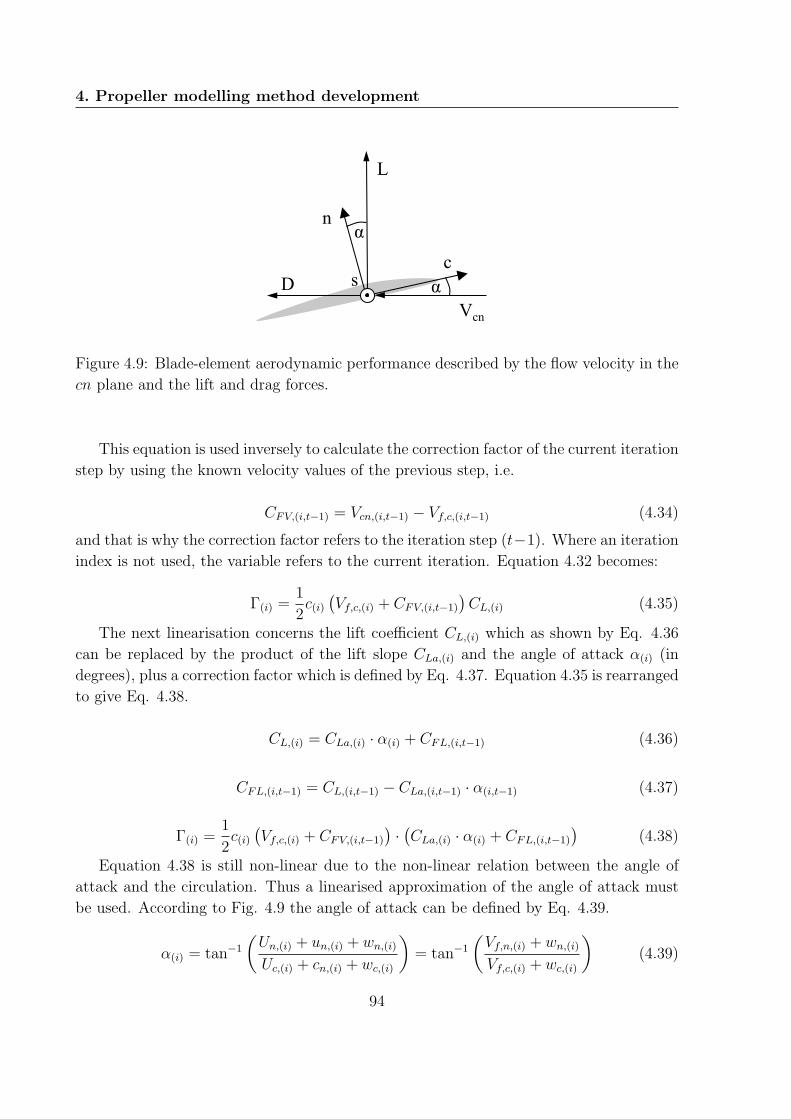
4. Propeller modelling method development

c

n

s Vcn

α D

L

α

Figure 4.9: Blade-element aerodynamic performance described by the flow velocity in the

cn plane and the lift and drag forces.

This equation is used inversely to calculate the correction factor of the current iteration

step by using the known velocity values of the previous step, i.e.

CFV,(i,t−1) = Vcn,(i,t−1) − Vf,c,(i,t−1) (4.34)

and that is why the correction factor refers to the iteration step (t−1). Where an iteration

index is not used, the variable refers to the current iteration. Equation 4.32 becomes:

Γ(i) =1

2c(i)(Vf,c,(i) + CFV,(i,t−1)

)CL,(i) (4.35)

The next linearisation concerns the lift coefficient CL,(i) which as shown by Eq. 4.36

can be replaced by the product of the lift slope CLa,(i) and the angle of attack α(i) (in

degrees), plus a correction factor which is defined by Eq. 4.37. Equation 4.35 is rearranged

to give Eq. 4.38.

CL,(i) = CLa,(i) · α(i) + CFL,(i,t−1) (4.36)

CFL,(i,t−1) = CL,(i,t−1) − CLa,(i,t−1) · α(i,t−1) (4.37)

Γ(i) =1

2c(i)(Vf,c,(i) + CFV,(i,t−1)

)·(CLa,(i) · α(i) + CFL,(i,t−1)

)(4.38)

Equation 4.38 is still non-linear due to the non-linear relation between the angle of

attack and the circulation. Thus a linearised approximation of the angle of attack must

be used. According to Fig. 4.9 the angle of attack can be defined by Eq. 4.39.

α(i) = tan−1

(Un,(i) + un,(i) + wn,(i)Uc,(i) + cn,(i) + wc,(i)

)= tan−1

(Vf,n,(i) + wn,(i)Vf,c,(i) + wc,(i)

)(4.39)

94

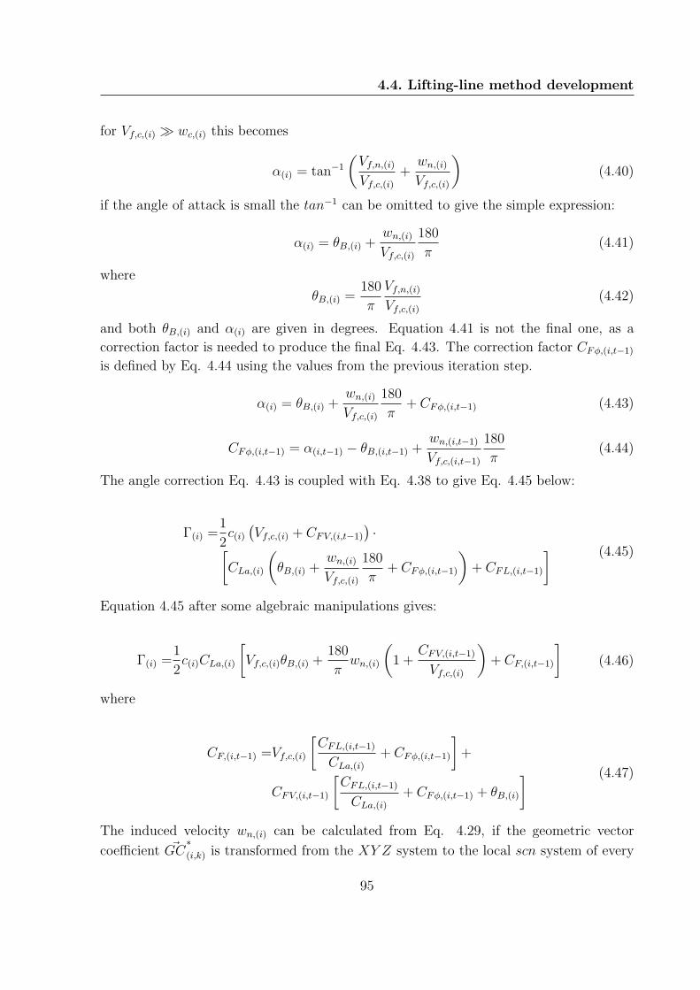
4.4. Lifting-line method development

for Vf,c,(i) wc,(i) this becomes

α(i) = tan−1

(Vf,n,(i)Vf,c,(i)

+wn,(i)Vf,c,(i)

)(4.40)

if the angle of attack is small the tan−1 can be omitted to give the simple expression:

α(i) = θB,(i) +wn,(i)Vf,c,(i)

180

π(4.41)

where

θB,(i) =180

π

Vf,n,(i)Vf,c,(i)

(4.42)

and both θB,(i) and α(i) are given in degrees. Equation 4.41 is not the final one, as a

correction factor is needed to produce the final Eq. 4.43. The correction factor CFφ,(i,t−1)

is defined by Eq. 4.44 using the values from the previous iteration step.

α(i) = θB,(i) +wn,(i)Vf,c,(i)

180

π+ CFφ,(i,t−1) (4.43)

CFφ,(i,t−1) = α(i,t−1) − θB,(i,t−1) +wn,(i,t−1)

Vf,c,(i,t−1)

180

π(4.44)

The angle correction Eq. 4.43 is coupled with Eq. 4.38 to give Eq. 4.45 below:

Γ(i) =1

2c(i)(Vf,c,(i) + CFV,(i,t−1)

)·[

CLa,(i)

(θB,(i) +

wn,(i)Vf,c,(i)

180

π+ CFφ,(i,t−1)

)+ CFL,(i,t−1)

] (4.45)

Equation 4.45 after some algebraic manipulations gives:

Γ(i) =1

2c(i)CLa,(i)

[Vf,c,(i)θB,(i) +

180

πwn,(i)

(1 +

CFV,(i,t−1)

Vf,c,(i)

)+ CF,(i,t−1)

](4.46)

where

CF,(i,t−1) =Vf,c,(i)

[CFL,(i,t−1)

CLa,(i)+ CFφ,(i,t−1)

]+

CFV,(i,t−1)

[CFL,(i,t−1)

CLa,(i)+ CFφ,(i,t−1) + θB,(i)

] (4.47)

The induced velocity wn,(i) can be calculated from Eq. 4.29, if the geometric vector

coefficient ~GC∗(i,k) is transformed from the XY Z system to the local scn system of every

95

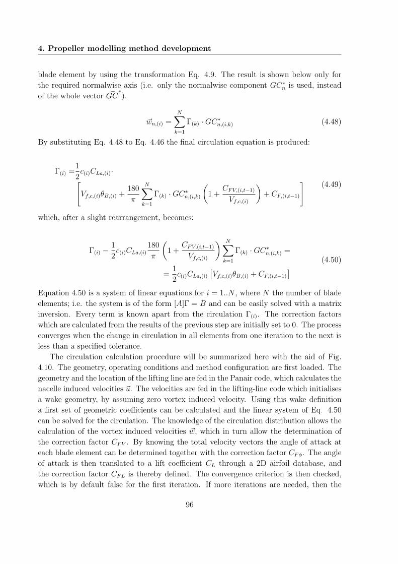
4. Propeller modelling method development

blade element by using the transformation Eq. 4.9. The result is shown below only for

the required normalwise axis (i.e. only the normalwise component GC∗n is used, instead

of the whole vector ~GC∗).

~wn,(i) =N∑k=1

Γ(k) ·GC∗n,(i,k) (4.48)

By substituting Eq. 4.48 to Eq. 4.46 the final circulation equation is produced:

Γ(i) =1

2c(i)CLa,(i)·[Vf,c,(i)θB,(i) +

180

π

N∑k=1

Γ(k) ·GC∗n,(i,k)(

1 +CFV,(i,t−1)

Vf,c,(i)

)+ CF,(i,t−1)

](4.49)

which, after a slight rearrangement, becomes:

Γ(i) −1

2c(i)CLa,(i)

180

π

(1 +

CFV,(i,t−1)

Vf,c,(i)

) N∑k=1

Γ(k) ·GC∗n,(i,k) =

=1

2c(i)CLa,(i)

[Vf,c,(i)θB,(i) + CF,(i,t−1)

] (4.50)

Equation 4.50 is a system of linear equations for i = 1..N , where N the number of blade

elements; i.e. the system is of the form [A]Γ = B and can be easily solved with a matrix

inversion. Every term is known apart from the circulation Γ(i). The correction factors

which are calculated from the results of the previous step are initially set to 0. The process

converges when the change in circulation in all elements from one iteration to the next is

less than a specified tolerance.

The circulation calculation procedure will be summarized here with the aid of Fig.

4.10. The geometry, operating conditions and method configuration are first loaded. The

geometry and the location of the lifting line are fed in the Panair code, which calculates the

nacelle induced velocities ~u. The velocities are fed in the lifting-line code which initialises

a wake geometry, by assuming zero vortex induced velocity. Using this wake definition

a first set of geometric coefficients can be calculated and the linear system of Eq. 4.50

can be solved for the circulation. The knowledge of the circulation distribution allows the

calculation of the vortex induced velocities ~w, which in turn allow the determination of

the correction factor CFV . By knowing the total velocity vectors the angle of attack at

each blade element can be determined together with the correction factor CFφ. The angle

of attack is then translated to a lift coefficient CL through a 2D airfoil database, and

the correction factor CFL is thereby defined. The convergence criterion is then checked,

which is by default false for the first iteration. If more iterations are needed, then the

96

4.4. Lifting-line method development

Read Input Prescribe wake geometry

Biot-Savart induced velocities

CFV

PANAIR nacelle flow

Calculate angle of attack

CFφ

YES

End calculations

NO

2D airfoil data CL à CFL

Update wake & CF

Γ(t ) −Γ(t−1) ≤ Tolerance

Calculate [A]Γ = B

Biot-Savart GC

Update wake? NO

Update CF

YES

Figure 4.10: Overview of the blade circulation calculation process.

wake geometry is updated by taking into account the new velocity field as described in

section 4.4.3 and the new geometric coefficients are calculated. The newly calculated

factors are also used to update the system of Eq. 4.50. The wake geometry does not need

to be updated more than approximately 3 times as further updates have a minor effect on

the results and consume excessive computational resources. If the process converges the

code passes to the final stage, which is the calculation of the lift and drag forces, which

are then translated to thrust, torque and efficiency, as described in the next section.

4.4.7 Blade-element performance

The lift and drag forces in Fig. 4.9 can be calculated by using a 2D airfoil database. This

database relates the angle of attack and Mach number of the flow with a lift and drag

coefficient CL and CD, which can then be used to calculate the lift L and drag D. The

2D airfoil database used in this analysis is the one reported in References [99], [138] and

[139]. This is probably the only one existing in the public domain which at the same time

is so extensive. It contains CL and CD data for the NACA-16 and NACA-65 families,

which are the ones commonly used in high-speed propellers. It covers Mach numbers

upto 1.6 and angles of attack from -4. to +8 degrees. The data do not include the post-

stall performance, therefore the performance prediction at operating conditions where a

97

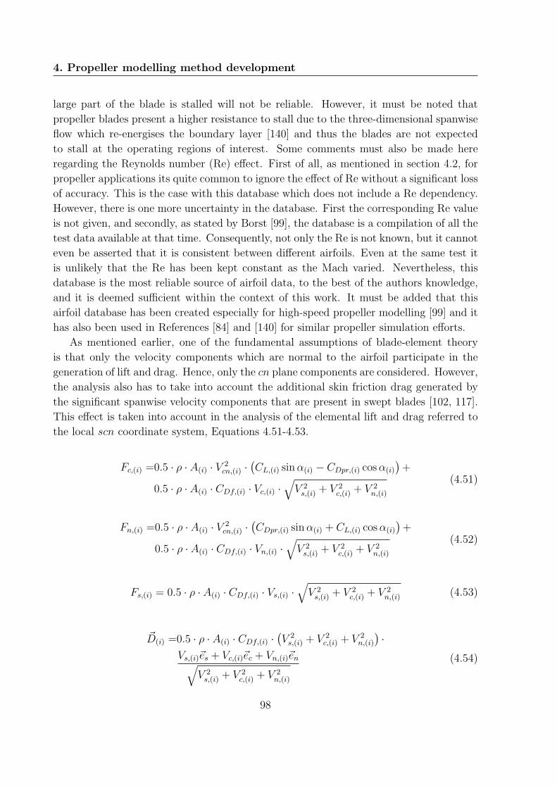
4. Propeller modelling method development

large part of the blade is stalled will not be reliable. However, it must be noted that

propeller blades present a higher resistance to stall due to the three-dimensional spanwise

flow which re-energises the boundary layer [140] and thus the blades are not expected

to stall at the operating regions of interest. Some comments must also be made here

regarding the Reynolds number (Re) effect. First of all, as mentioned in section 4.2, for

propeller applications its quite common to ignore the effect of Re without a significant loss

of accuracy. This is the case with this database which does not include a Re dependency.

However, there is one more uncertainty in the database. First the corresponding Re value

is not given, and secondly, as stated by Borst [99], the database is a compilation of all the

test data available at that time. Consequently, not only the Re is not known, but it cannot

even be asserted that it is consistent between different airfoils. Even at the same test it

is unlikely that the Re has been kept constant as the Mach varied. Nevertheless, this

database is the most reliable source of airfoil data, to the best of the authors knowledge,

and it is deemed sufficient within the context of this work. It must be added that this

airfoil database has been created especially for high-speed propeller modelling [99] and it

has also been used in References [84] and [140] for similar propeller simulation efforts.

As mentioned earlier, one of the fundamental assumptions of blade-element theory

is that only the velocity components which are normal to the airfoil participate in the

generation of lift and drag. Hence, only the cn plane components are considered. However,

the analysis also has to take into account the additional skin friction drag generated by

the significant spanwise velocity components that are present in swept blades [102, 117].

This effect is taken into account in the analysis of the elemental lift and drag referred to

the local scn coordinate system, Equations 4.51-4.53.

Fc,(i) =0.5 · ρ · A(i) · V 2cn,(i) ·

(CL,(i) sinα(i) − CDpr,(i) cosα(i)

)+

0.5 · ρ · A(i) · CDf,(i) · Vc,(i) ·√V 2s,(i) + V 2

c,(i) + V 2n,(i)

(4.51)

Fn,(i) =0.5 · ρ · A(i) · V 2cn,(i) ·

(CDpr,(i) sinα(i) + CL,(i) cosα(i)

)+

0.5 · ρ · A(i) · CDf,(i) · Vn,(i) ·√V 2s,(i) + V 2

c,(i) + V 2n,(i)

(4.52)

Fs,(i) = 0.5 · ρ · A(i) · CDf,(i) · Vs,(i) ·√V 2s,(i) + V 2

c,(i) + V 2n,(i) (4.53)

~D(i) =0.5 · ρ · A(i) · CDf,(i) ·(V 2s,(i) + V 2

c,(i) + V 2n,(i)

)·

Vs,(i)~es + Vc,(i)~ec + Vn,(i)~en√V 2s,(i) + V 2

c,(i) + V 2n,(i)

(4.54)

98

4.4. Lifting-line method development

In the above equations, A(i) is the area of the blade element i, CDpr is the pressure

drag coefficient and CDf the friction drag coefficient. This distinction between pressure

and friction drag is made for the following reason. The pressure drag is only a result

of the flow in the 2D cn plane, while the friction drag must also take into account the

spanwise velocity component. Hence, the friction drag acts in the direction of the total

velocity vector, while the pressure drag acts in the direction of the velocity ~Vcn that lies

in the cn plane. This concept is represented by Eq. 4.54 which defines the friction drag

vector. The term in the second line of the equation is the total velocity vector divided

by its magnitude in order to give a unit vector. The spanwise force Fs includes the

projection of the total friction drag to the spanwise direction, while the projections to the

chordwise and normalwise axes are included as additional terms in the calculation of the

force components Fc and Fn, Eq. 4.51 and Eq. 4.52. A last point must be made regarding

the pressure and friction drag coefficients. The available airfoil database only gives a total

drag coefficient CD without differentiating between pressure and friction drag. According

to Egolf et al [117] the friction drag coefficient CDf can be approximated by the total

drag coefficient for zero angle of attack; i.e. CDf = CD(α = 0). Then the pressure drag

coefficient can be given by, CDpr = CD − CDf .

~F(i) = Fs,(i) · ~es + Fc,(i) · ~ec + Fn,(i) · ~en (4.55)

~F(i) = FX,(i) · ~eX + FY,(i) · ~eY + FZ,(i) · ~eZ (4.56)

The element force analysis results in the final definition of the total force vector in

the local scn system (Eq. 4.55), which can then be translated to the global XY Z system

(Eq. 4.56) by using Eq. 4.10. The element thrust is then equal to the Z component of

the force vector (Eq. 4.57), while the torque is calculated by the external product of the

force and position vector, projected to the Z axis (Eq. 4.58). The position vector refers to

the center (in the spanwise direction) of the blade element located on the quarter chord

line of the blade.

T(i) = FZ,(i) (4.57)

Q(i) =(~F(i) × ~rBE,(i)

)· ~eZ = FX,(i) · rBE,Y,(i) − FY,(i) · rBE,X,(i) (4.58)

The total thrust and torque can now be calculated by Eq. 4.59 and Eq. 4.60 by a

simple summation of the thrust of all the blade elements times the number of blades M .

The propeller power is then given by Eq. 4.61 and the efficiency by Eq. 4.62, where

Ω is the propeller rotational speed in [rad/s] and V0 is the flight velocity in [m/s]. The

calculation of the propeller performance has been completed.

99

4. Propeller modelling method development

T = NB ·N∑i=1

T(i) (4.59)

Q = NB ·N∑i=1

Q(i) (4.60)

P = Q · Ω (4.61)

ηprop =T · V0

P(4.62)

4.4.8 Compressibility effects

As confirmed by the literature survey of section 4.3, lifting-line methods similar to the

one developed in the previous sections are the current state-of-the-art for prop-fan prelim-

inary analysis and design. One of the very fundamental assumptions in the development

of the lifting-line approach, is the hypothesis of a potential, incompressible flow [96]. This

hypothesis, which is shared with the panel methods, leads to a convenient linear differ-

ential equation that describes the flow under investigation. The greatest advantage of a

linear differential equation is that, if a set of solutions is known, any linear combination

of this solution is also a solution [132]. The effect of a single straight vortex segment is

an elementary solution (or singularity), which combined with the effect of all the other

vortex segments through a simple summation gives the total flow velocities solution (see

section 4.4.5).

Contrary to the lifting-line, which is strictly incompressible, the panel methods have

been extended to compressible subsonic and supersonic applications without losing their

linearity. The difference between subsonic and supersonic was described by Von Karman

[141]. For subsonic flows the effect of a singularity, such as a vortex segment, is felt in

the whole computational domain, while for supersonic flows it is only affecting regions

within its aft Mach cone. This is what Von Karman called the ”zone of action”, while

what is outside is called the ”zone of silence”. From a mathematical perspective the equa-

tion of the subsonic problem is of the elliptic type, while the supersonic flow equation is

hyperbolic [137]. Unfortunately, a propeller usually operates in a completely transonic

flow, where the hub Mach number is close to 0.8 and the tip close to 1.2. Anderson [96]

explicitly states that a linearised solution is not valid in this range of Mach number. This

is confirmed by Nixon (in Morino’s edition [133]), who suggests that even the most prim-

itive representation of the flow still requires a non-linear equation. From a mathematical

perspective a transonic equation is of a mixed elliptic/hyperbolic type. Non-linear equa-

tions can only be solved by discretising the whole fluid volume and by solving with partial

100

4.4. Lifting-line method development

differences or other relevant methods that belong to the domain of CFD but not in the

group of panel methods.

Despite the aforementioned difficulties, a few works where found in the literature

that attempted to add some transonic capability to a linear propeller simulation method.

The works will be commented in approximately chronological order. Davidson in 1953

[142] proposed a linearised solution to the potential problem for ducted fans. Wells [143]

extended his work to the case of unducted propellers. There are three main problems with

their approach. First the authors do not justify the linearisation of an equation which

normally is not allowed to be linearised. Secondly, they did not report any results to

prove the modelling reliability and fidelity of their approach. And thirdly, their approach

follows the Goldstein [97] method, and thus it is only applicable to straight blades with

rigid helical wakes. This assumption is not adequate for the case of prop-fan modelling

as discussed in sections 4.3 and 4.4.3.

A different path was followed by Borst [99] who proposed two corrections applied

to his baseline Goldstein/Theodorsen method. The same corrections were applied later

by Egolf [117] and Rohrbach [105] to a lifting-line method. The first correction is an

application of the ”zones of silence” concept to the calculation of induced velocities as

presented in sections 4.4.4 and 4.4.5. According to Borst, when summing the influence of

every single vortex segment, one must only take into account the vortex segments which

are inside the ”zone of action”. This is tested simply by checking whether the signal that

was emitted from the location of the segment had the time to reach the current location

of the blade element. As a result, the initial segments of a trailing vortex filament are

likely to be outside the zone of action and therefore have no effect on the velocity. The

second modification suggested by Borst was the application of a correction factor within

the Mach cone of the tip of the blade. This was implemented by using results from a

supersonic potential calculation conducted for a fixed wing flying with a constant speed

along the span as reported by Evvard [144]. The estimated correction factors where

applied on the lift and drag coefficients. The supersonic calculation by Evvard already

includes the concept of hyperbolic flow and ”zones of silence” and therefore it appears that

the two corrections overlap. Furthermore, the calculation by Evvard was dealing with a

completely supersonic flow of a wing and its applicability to a rotating transonic propeller

is not justified. Finally, the combination of the ”zones of silence” concept with the strictly

incompressible Biot-Savart law is quite dubious. Therefore, the two modifications can

only be seen as ”engineering corrections”, which attempt to model some real phenomena,

but in a way that is not formally proven or justified. The concerns over validity of the

correction are confirmed by the results from both studies [105] and [117]. The predictions

seem unrealistic as they present a reversal of curvature in the efficiency-Mach curve after a

Mach number of 0.80 (Fig. 4.11). This happens because of the de-activation of the vortex

segments located close to the blade and outside the ”zones of action”, with a parallel

101

4. Propeller modelling method development

reduction in ideal losses. At this point it is worth drawing the attention of the reader to

the fact that Reference [105] was written by Hamilton Standard which is the company

that designed the SR family of prop-fans. This fact highlights that the task of prop-fan

modelling is far from being trivial.

0.6 0.65 0.7 0.75 0.8 0.85 0.976

77

78

79

80

81

82

Flight Mach

Prop

elle

r Effi

cien

cy [%

]

Figure 4.11: Efficiency prediction results from Rohrbach et al [105] using the Borst cor-

rections. Prediction for the SR3 propeller, J = 3.06 and CP = 1.695. Unrealistic change

of curvature after Mach = 0.80.

The work of Hanson (also working in Hamilton Standard) in the 80s [83, 145, 146] is

the most complete found by the author, and the only one that has a formal mathematical

and physical formulation. Hanson built a lifting-surface method based on the linear

wave equation in order to produce unsteady results for noise calculations. The method

could also work in steady state for aerodynamic calculations and Hanson claimed that his

prop-fan performance prediction was the most accurate at that time. The use of a linear

equation was justified by using a criterion found in Bisplinghoff et al [147] and reproduced

below:

AR3 · δ ·[ln(ARδ1/3

)]2 1 (4.63)

where AR is the blade aspect ratio and δ the thickness ratio. By using the values AR =

3 and δ = 0.02, which are typical of a prop-fan blade, Hanson calculated a value of

AR3δ[ln(ARδ1/3

)]2equal to 0.023. This value satisfies the criterion of Eq. 4.63 and

justifies the use of a linearised theory. Indeed the results at high Mach number looked

promising but this was not the case for the low Mach number predictions. The theory

assumed that the blades travel on a rigid helical wake and therefore did not take into

102

4.4. Lifting-line method development

account the effect of induced velocities on the wake. This effect introduced an important

non-linearity to the flow which was not captured by the model. An attempt to rectify

the problem was made through a coupling with a momentum theory but the results as

reported by Hanson et al [83] were still unsatisfactory. Nevertheless, the high speed results

will be kept as a reference base for the validation of this work. Another very interesting

finding of his work, and more specifically of Reference [146], is the justification of using a

simple lifting-line theory. By using a formal mathematical approach Hanson proved that

the effect of modelling the blade with a single lifting line (thus neglecting the chordwise

variations) cancels out with the effect of the incompressibility hypothesis. According to

Hanson [146] this is the reason that lifting-line methods have been so successful in the

design of prop-fans.

The most recent work found in the literature relative to the treatment of compressibil-

ity is the approach of Szymendera [135], which was also followed by Burger [129]. In this

case, Szymendera assumed that each vortex segment performs an independent motion

away from the control point which is located on the blade-element. He then performed

a simple Prandtl-Glauert transformation of the domain to capture the stretching of the

space due to compressibility as described in Anderson [96]. However, the treatment of

each vortex segment as a separate flow was not justified by the author, and his results for

the compressible case were less accurate than without the compressibility modification.

Therefore, the suggested approach does not seem reliable.

Following this literature survey, it has been decided to follow a completely incompress-

ible approach for the calculation of the vortex induced velocities; i.e. no modification is

required to what has already been presented in the previous sections. This decision is

based on: 1) the complexity of implementing Hanson’s method which seems as the most

well formulated, 2) the unsatisfactory results of the same method at take-off conditions, 3)

the last argument of Hanson [146] regarding the suitability of simple lifting-line methods.

As mentioned earlier, the high speed results of Hanson et al [83] will be kept as a compar-

ison base for the validation of the method implemented. This will permit the evaluation

of the error introduced by using a simpler modelling approach instead of a higher fidelity

one. At the same time, it must be reminded that a part of the compressibility effects

is captured through the airfoil database which includes the lift and drag coefficients as

functions of Mach number. Furthermore, it must also be underlined that PANAIR models

the compressible subsonic flow around the spinner/nacelle, although it has been decided

to limit the input Mach number to 0.7. This has been done in order to ensure that the

code operates in the Mach number domain suitable for linear potential theory (the upper

limit being 0.7-0.8).

103

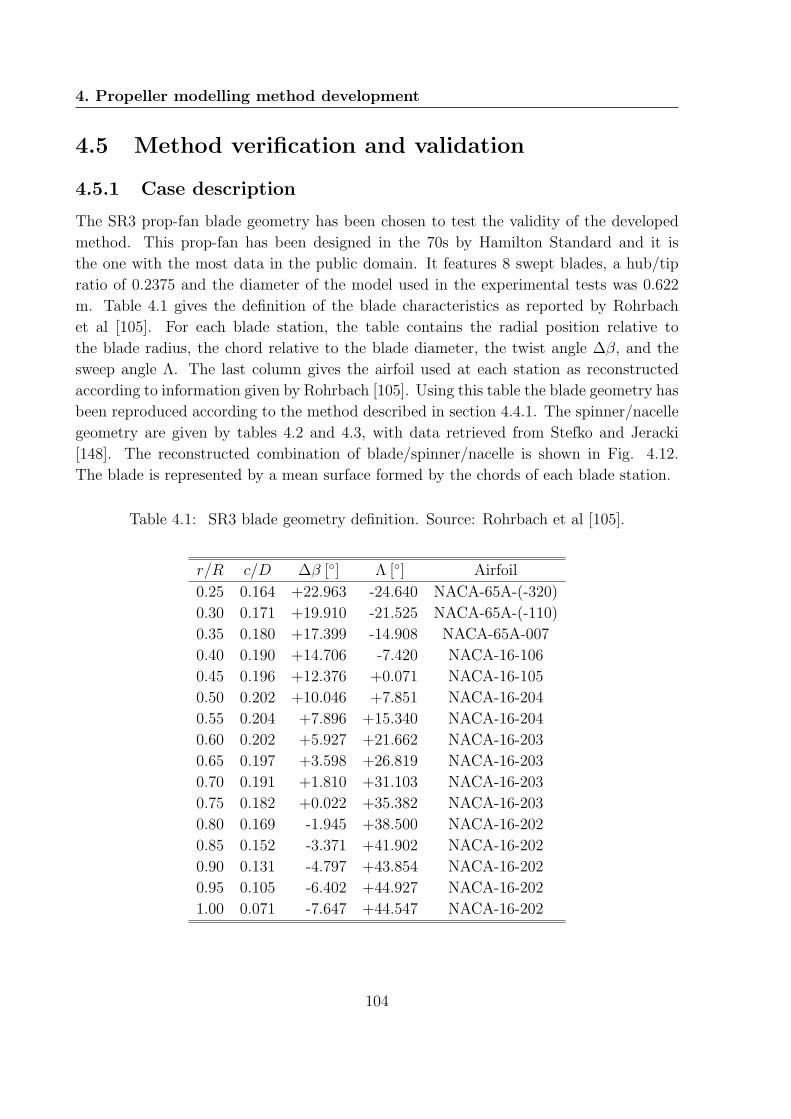
4. Propeller modelling method development

4.5 Method verification and validation

4.5.1 Case description

The SR3 prop-fan blade geometry has been chosen to test the validity of the developed

method. This prop-fan has been designed in the 70s by Hamilton Standard and it is

the one with the most data in the public domain. It features 8 swept blades, a hub/tip

ratio of 0.2375 and the diameter of the model used in the experimental tests was 0.622

m. Table 4.1 gives the definition of the blade characteristics as reported by Rohrbach

et al [105]. For each blade station, the table contains the radial position relative to

the blade radius, the chord relative to the blade diameter, the twist angle ∆β, and the

sweep angle Λ. The last column gives the airfoil used at each station as reconstructed

according to information given by Rohrbach [105]. Using this table the blade geometry has

been reproduced according to the method described in section 4.4.1. The spinner/nacelle

geometry are given by tables 4.2 and 4.3, with data retrieved from Stefko and Jeracki

[148]. The reconstructed combination of blade/spinner/nacelle is shown in Fig. 4.12.

The blade is represented by a mean surface formed by the chords of each blade station.

Table 4.1: SR3 blade geometry definition. Source: Rohrbach et al [105].

r/R c/D ∆β [] Λ [] Airfoil

0.25 0.164 +22.963 -24.640 NACA-65A-(-320)

0.30 0.171 +19.910 -21.525 NACA-65A-(-110)

0.35 0.180 +17.399 -14.908 NACA-65A-007

0.40 0.190 +14.706 -7.420 NACA-16-106

0.45 0.196 +12.376 +0.071 NACA-16-105

0.50 0.202 +10.046 +7.851 NACA-16-204

0.55 0.204 +7.896 +15.340 NACA-16-204

0.60 0.202 +5.927 +21.662 NACA-16-203

0.65 0.197 +3.598 +26.819 NACA-16-203

0.70 0.191 +1.810 +31.103 NACA-16-203

0.75 0.182 +0.022 +35.382 NACA-16-203

0.80 0.169 -1.945 +38.500 NACA-16-202

0.85 0.152 -3.371 +41.902 NACA-16-202

0.90 0.131 -4.797 +43.854 NACA-16-202

0.95 0.105 -6.402 +44.927 NACA-16-202

1.00 0.071 -7.647 +44.547 NACA-16-202

104

4.5. Method verification and validation

Table 4.2: SR3 spinner geometry definition. Rref = 0.1105. Source: Stefko and Jeracki

[148].

x/Rref r/Rref x/Rref r/Rref

0.000 0.000 1.207 0.598

0.081 0.119 1.264 0.597

0.138 0.168 1.322 0.595

0.253 0.246 1.379 0.597

0.368 0.310 1.437 0.606

0.598 0.410 1.494 0.619

0.828 0.497 1.552 0.636

1.057 0.568 1.609 0.654

1.092 0.577 1.667 0.673

1.149 0.591 2.184 0.857

Table 4.3: SR3 nacelle geometry definition. Rref = 0.1105. Source: Stefko and Jeracki

[148].

x/Rref r/Rref x/Rref r/Rref

2.199 0.860 3.136 0.999

2.216 0.866 3.214 1.000

2.239 0.873 3.366 0.999

2.262 0.881 3.596 0.990

2.285 0.888 3.825 0.975

2.308 0.895 4.055 0.956

2.331 0.902 4.285 0.933

2.354 0.908 4.515 0.911

2.377 0.915 4.745 0.894

2.400 0.920 4.975 0.883

2.423 0.926 5.205 0.874

2.446 0.931 5.251 0.873

2.561 0.946 5.297 0.871

2.676 0.970 5.400 0.871

2.791 0.982 5.417 0.865

2.906 0.990 8.659 1.046

105

4. Propeller modelling method development

X

Z Y

X

Y

Z

Figure 4.12: The SR3 blade/spinner/nacelle geometry as reconstructed by the developed

code.

4.5.2 Model configuration

The set-up of the numerical model is given in table 4.4. The choice of the grid parameters is

a result of a grid parametric study as shown in figures 4.13-4.14. The choice of 20 spanwise

blade stations is in line with what is reported by Burger [129], while the respective grading

parameter was chosen to give a denser distribution close to the blade tip. Traumel [134]

suggested that only the first turn of the wake needs to be accounted for, while the rest of

the wake can be taken into account by approximative methods. This statement is in part

confirmed by Fig. 4.13b which shows that after two turns the result does not change. This

is logical, as it is the wake segments closest to the blade that have the greatest impact

on the performance. However, it has been decided to include four wake turns in order

to accommodate cases where the advance ratio is low and therefore the wake segments

are closer to the blades for the same number of turns. Once more, the wake azimuthal

grading factor was set to 1.6, resulting in smaller segments close to the blades where the

greatest accuracy is needed. For the same reason the wake points number has to be kept

over 100 as shown by Fig. 4.13c; the smaller the wake vortex segments, the greater the

accuracy of the induced velocities calculation. This wake configuration results in a first

wake azimuthal angle less than 1 degree as recommended by Traumel [134] and Leishman

[127].

Section 4.4.3 discussed the importance of taking into account the induced velocities

in the calculation of the wake geometry. In section 4.4.8 this was also confirmed by the

work of Hanson [83], who attempted to couple his high-fidelity code with a momentum

model in order to capture this effect. Figure 4.13d is another proof that this statement

106

4.5. Method verification and validation

Table 4.4: Model configuration.

Parameter Value

Number of blade grid spanwise stations 20

Wake turns 4

Number of wake azimuthal points 100

Blade radial grading parameter 1.2

Wake azimuthal grading parameter 1.6

Number of wake updates 3

Number of nacelle grid axial points 50

Number of nacelle grid azimuthal points 10

Nacelle azimuthal grading parameter 1.6

Circulation convergence tolerance 10−10

holds true. A set-up with zero wake updates results in a wake that assumes a rigid

helix form, where the vortex induced velocities are not taken into account. This leads to

vortex segments that are closer to the blades, induce higher velocities and result in a lower

efficiency. As soon as the wake is updated to account for the induced velocities, the vortex

segments start moving further from the blades due to their own induced velocities and the

efficiency increases. As shown in Fig. 4.13d two to three wake updates are enough to have

an accurate prediction, result identical to what was reported by Young [123]. Regarding

the spinner/nacelle grid, Fig. 4.14a shows that at least 50 axial elements are needed,

with a grading value of 1.6 that results in a denser grid close to the spinner nose. Due

to the axi-symmetric shape of the spinner/nacelle only a quadrant needs to be modelled,

with at least 10 azimuthal elements as shown by Fig. 4.14b. The resulting grid for the

combination of blade, wake, spinner and nacelle is shown in Fig. 4.15.

A last point needs to be underlined here regarding the model set-up for the simula-

tion of the SR3 prop-fan. The blades used in the experimental tests are not completely

rigid and present some elastic deformation in their twist angles; i.e. the blades tend to

”detwist”. This was reported by many studies in the open literature [80, 82, 83, 105, 111,

112, 149]. Bober et al [149] calculated the deformation for an operating point where the

prop-fan rotated at 8440 rpm using a finite element analysis. The produced distribution of

detwist along the blade was then used at other speeds, scaled by the square of rotational

speed. As it will be shown in the next section, this detwisting effect has an important

impact on performance and therefore it has to be taken into account for the comparison

with the SR3 data. The results of Bober et al [149] were retrieved from Bober and Chang

[111] and fitted by the curve given in Eq. 4.64. This curve is used in the model in order

107

4. Propeller modelling method development

to compare with the experimental data in the next sections.

detwist =[−2.8964(r/R)2 + 5.4457(r/R)− 0.959

]· (RPM/8440)2 (4.64)

4.5.3 Results

The first set of results presented in figure 4.16 verifies the modelling of the detwisting

deformations effect. Figure 4.16a and Fig. 4.16b represent low Mach number conditions

(M=0.2), while Fig. 4.16c and Fig. 4.16d depict the effect at high Mach conditions

(M=0.8). Bober et al [111] reported that for the same conditions as Fig. 4.16c, an increase

of CP between 0.22 and 0.36 was observed for a rigid blade relative to a deformable one.

Figure 4.16c shows a difference between 0.197 and 0.235. The effect is in the same order of

magnitude but slightly under-predicted. The uncertainties in the actual aerodynamic and

deformations modelling approach of Bober and Chang [111] do not allow further comments

and the result is found satisfactory. According to Fig. 4.16d the increase in efficiency for

the deformed blade is 3.2%, which again is in line with the 4% reported by Bober and

Chang [111]. An interesting observation can be made if one studies the same effect for

low Mach number this time. As shown by Fig. 4.16a and Fig. 4.16b the deformations

impact is much lower for low Mach numbers. This can be explained by observing the

change in the slope of the CL−angle curves for increasing Mach number (Fig. 4.17). The

higher the Mach number the higher the slope of the curve and thus a change in angle of

attack results in a higher change in performance for high Mach conditions. A detwisting

deformation under constant advance ratio J , i.e. constant free stream velocity vector,

results in a change in the blade angle and thus in the angle of attack. This change in the

angle of attack is then translated to a lower change in CP for lower Mach numbers and a

higher CP change for high Mach numbers.

The next step consists in verifying the accurate modelling of the flow around the

spinner and nacelle. Egolf et al [117] quoted measured values of Mach number in the

plane Z/Lref = 0.09 for an operating Mach number Mref = 0.8. The parameter Z

represents the axial distance from the nose of the spinner. Figure 4.18 shows that PAN

AIR is matching well the experimental data, especially in the high power outboard region

of the blade. The inboard areas are less important because they are less loaded and thus

affect less the performance.

The developed code was subsequently used in order to produce data in the form of

propeller maps. These maps consist of lines of constant pitch angle, for different advance

ratios. Each different advance ratio results in a different power coefficient and propeller

efficiency. First the predicting capability for low Mach performance is compared in Fig.

4.19a and Fig. 4.19b against experimental data extracted from Stefko and Jeracki [148].

Both the power coefficient and efficiency compare very well with the test data, with higher

108

4.5. Method verification and validation

0 5 10 15 20 25 300.78

0.782

0.784

0.786

0.788

0.79

0.792

0.794

Blade spanwise stations number

Prop

elle

r Effi

cien

cy

(a) Number of blade spanwise stations

0 2 4 6 80.788

0.7885

0.789

0.7895

0.79

Wake turns numberPr

opel

ler E

ffici

ency

(b) Number of wake turns calculated

0 50 100 1500.787

0.788

0.789

0.79

0.791

0.792

Wake points number

Prop

elle

r Effi

cien

cy

(c) Number of wake points calculated

0 1 2 3 4 50.78

0.782

0.784

0.786

0.788

0.79

Wake updates number

Prop

elle

r Effi

cien

cy

(d) Number of wake updates

Figure 4.13: Grid independency study for the propeller modelling parameters. Operating

conditions: M=0.8, J=3.06, Pitch=58.50. All parameters are set to the values of table

4.4.

109

4. Propeller modelling method development

0 10 20 30 40 50 60 700.787

0.7875

0.788

0.7885

0.789

0.7895

0.79

Nacelle axial points number

Prop

elle

r Effi

cien

cy

(a) Number of nacelle axial points

0 2 4 6 8 10 12 140.78

0.782

0.784

0.786

0.788

0.79

Nacelle azimuthal points number

Prop

elle

r Effi

cien

cy

(b) Number of nacelle azimuthal pointsper quadrant

Figure 4.14: Grid independency study for the nacelle/spinner modelling parameters. Op-

erating conditions: M=0.8, J=3.06, Pitch=58.50. All parameters are set to the values of

table 4.4.

Figure 4.15: The SR3 blade/spinner/nacelle/wake grid as discretised by the developed

code according to the settings given in table 4.4.

110

4.5. Method verification and validation

1 1.5 20.2

0.4

0.6

0.8

1

1.2

Advance ratio J

Pow

er c

oeffi

cien

t Cp

deformedrigid

(a) Power coefficientM=0.2, Pitch=41.9

1 1.5 20.5

0.55

0.6

0.65

0.7

0.75

0.8

0.85

0.9

Advance ratio J

Prop

elle

r effi

cien

cy

deformedrigid

(b) EfficiencyM=0.2, Pitch=41.9

3 3.5 40.5

1

1.5

2

2.5

3

Advance ratio J

Pow

er c

oeffi

cien

t Cp

deformedrigid

(c) Power coefficientM=0.8, Pitch=60.4

3 3.5 40.7

0.72

0.74

0.76

0.78

0.8

0.82

0.84

Advance ratio J

Prop

elle

r effi

cien

cy

deformedrigid

(d) EfficiencyM=0.8, Pitch=60.4

Figure 4.16: The effect of blade deformations on the power coefficient and efficiency.

111

4. Propeller modelling method development

ï2 0 2 4 60

0.2

0.4

0.6

0.8

1

Angle of attack [degrees]

C L

M = 0.3M = 0.86

Figure 4.17: The effect of Mach number on the lift coefficient CL for the NACA-16-204

airfoil.

0.2 0.4 0.6 0.8 10.7

0.75

0.8

0.85

0.9

0.95

1

Relative radius ï r/Lref

Rela

tive

Mac

h ï

M/M

ref

PAN AIR predictionExperimental data

Figure 4.18: Comparison of Mach number profile predicted by PAN AIR with test data ex-

tracted from Egolf et al [117]. Measurements taken at plane Z/Lref = 0.09 for Mref=0.8.

Lref=12.25 inches.

112

4.5. Method verification and validation

discrepancies occurring in the low advance ratios of the CP − J lines. In this operating

region the angles of attack are the highest and flow separation is very likely. As discussed

in 4.4.7 the airfoil data do not predict well the stalled operating regime, which can partly

explain the observed discrepancies. As shown by Fig. 4.20a and Fig. 4.20b the code also

matches very well the experimental data extracted from Jeracki et al [150] for M = 0.6.

However, this time the calculated angles had to be reduced by 1.5-2 degrees due to the

deformation effects which are higher for higher Mach numbers.

The predicted performance at the high speed condition M = 0.8 is compared in

Fig. 4.21 against experimental data from Rohrbach et al [105]. The predictions of the

compressible lifting-surface code by Hanson [83] are also shown. Both the developed

method and the Hanson code predict well the shape of the 59.3 iso-pitch line. The 57.3

is better predicted by the Hanson code, while the 60.5 is matched better by the developed

code. Similarly to the case of M = 0.6, there is a under-prediction of the pitch angles

by around 2 degrees. Hanson [83] reported that according to the experience of Hamilton

Standard these two degrees are attributed to the flexibility of the blade retention system.

Thus their effect is not included in the detwisting model of Eq. 4.64, which only includes

the deformations of the blade. The different predictions between the developed code

and the one by Hanson can either be due to different deformation models or due to the

differences in the aerodynamic modelling. As mentioned earlier, Hanson’s method better

captures the linear compressibility effects but lacks accuracy regarding the non-linear

impact of the induced velocities. These are better captured by the developed code, which

however does not model the effect of compressibility on the calculation of the induced

flow. The similar accuracies between the two approaches justifies the earlier selection

regarding the modelling of compressibility, as discussed in section 4.4.8. With the respect

to the propeller global performance prediction, a simple incompressible lifting-line method

is equally good with a higher-fidelity compressible lifting-surface model.

A way to partially eliminate the effect of deformations and focus on the effect of

compressibility is to predict the performance at given power coefficient and advance ratio;

i.e. leave the pitch angle out of the equation. Figure 4.22 attempts to perform this exercise

and compare against the ideal and measured real efficiencies quoted by Jeracki et al [150].

The ideal efficiency is the efficiency of the propeller for zero drag conditions, while the

no-induced efficiency is the efficiency with all the induced velocities set to zero; i.e. only

the viscous drag losses are taken into account. This is done in order to isolate the different

modelling features and check separately their predictive capability. The first conclusion

that can be drawn from Fig. 4.22 is that the ideal efficiency is very well predicted. That

shows that the wake modelling and the calculation of the induced velocities are quite

accurate. It must be underlined here that the value of the ideal efficiency is shown to be

constant because the impact of compressibility is not accounted for. In this case, as stated

by Mikkelson et al [80], the ideal efficiency is only a function of the power coefficient and

113

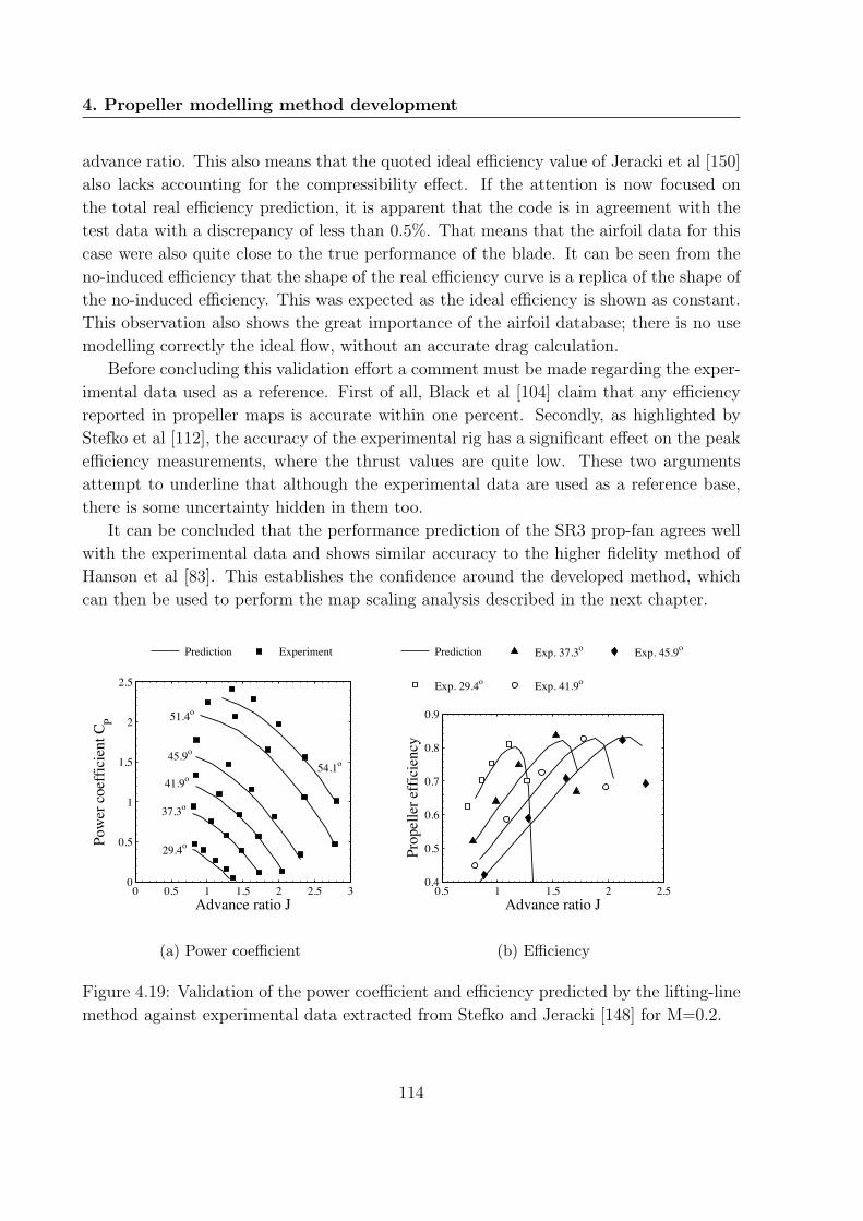
4. Propeller modelling method development

advance ratio. This also means that the quoted ideal efficiency value of Jeracki et al [150]

also lacks accounting for the compressibility effect. If the attention is now focused on

the total real efficiency prediction, it is apparent that the code is in agreement with the

test data with a discrepancy of less than 0.5%. That means that the airfoil data for this

case were also quite close to the true performance of the blade. It can be seen from the

no-induced efficiency that the shape of the real efficiency curve is a replica of the shape of

the no-induced efficiency. This was expected as the ideal efficiency is shown as constant.

This observation also shows the great importance of the airfoil database; there is no use

modelling correctly the ideal flow, without an accurate drag calculation.

Before concluding this validation effort a comment must be made regarding the exper-

imental data used as a reference. First of all, Black et al [104] claim that any efficiency

reported in propeller maps is accurate within one percent. Secondly, as highlighted by

Stefko et al [112], the accuracy of the experimental rig has a significant effect on the peak

efficiency measurements, where the thrust values are quite low. These two arguments

attempt to underline that although the experimental data are used as a reference base,

there is some uncertainty hidden in them too.

It can be concluded that the performance prediction of the SR3 prop-fan agrees well

with the experimental data and shows similar accuracy to the higher fidelity method of

Hanson et al [83]. This establishes the confidence around the developed method, which

can then be used to perform the map scaling analysis described in the next chapter.

0 0.5 1 1.5 2 2.5 30

0.5

1

1.5

2

2.5

Advance ratio J

Pow

er c

oeffi

cien

t CP

Prediction Experiment

29.4o

54.1o

37.3o

41.9o

45.9o

51.4o

(a) Power coefficient

0.5 1 1.5 2 2.50.4

0.5

0.6

0.7

0.8

0.9

Advance ratio J

Prop

elle

r effi

cien

cy

Prediction

Exp. 29.4o

Exp. 37.3o

Exp. 41.9o

Exp. 45.9o

(b) Efficiency

Figure 4.19: Validation of the power coefficient and efficiency predicted by the lifting-line

method against experimental data extracted from Stefko and Jeracki [148] for M=0.2.

114

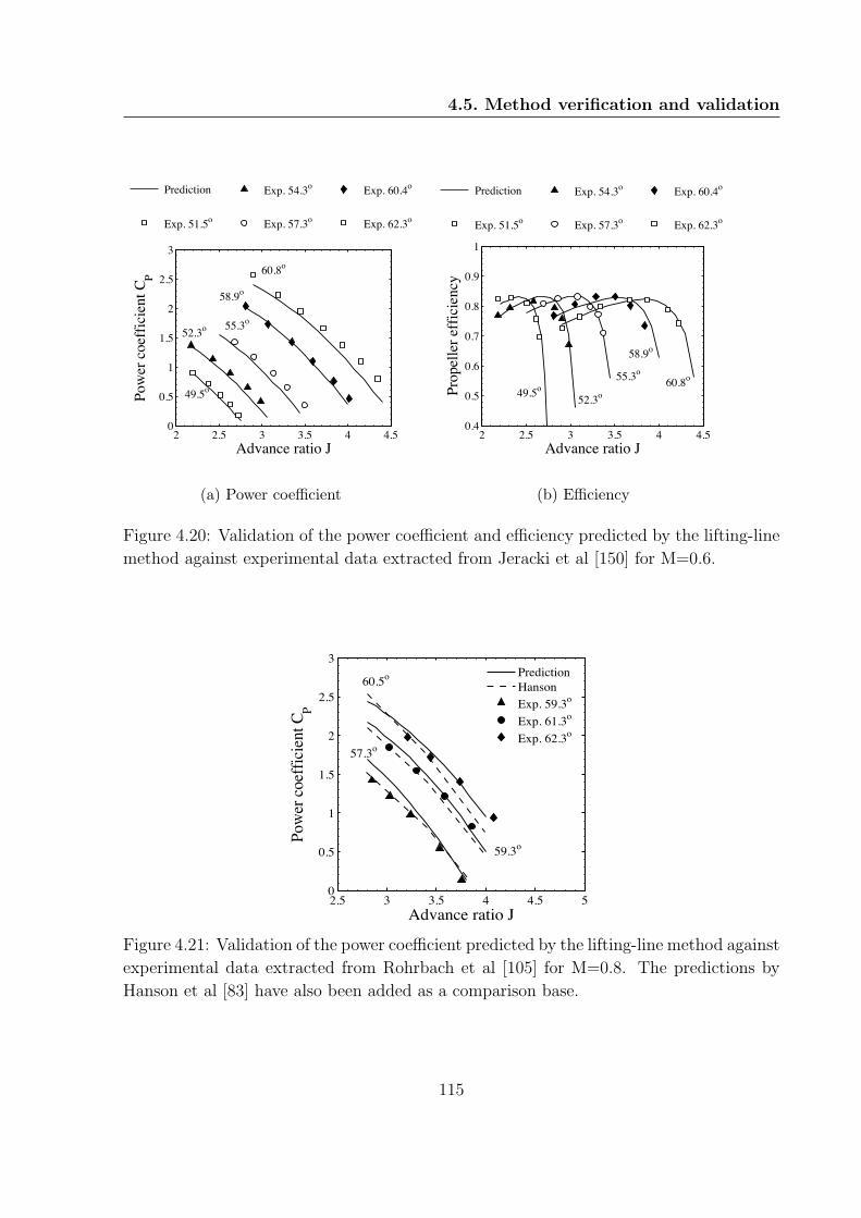
4.5. Method verification and validation

2 2.5 3 3.5 4 4.50

0.5

1

1.5

2

2.5

3

Advance ratio J

Pow

er c

oeffi

cien

t CP

Prediction

Exp. 51.5o

Exp. 54.3o

Exp. 57.3o

Exp. 60.4o

Exp. 62.3o

49.5o

52.3o

58.9o

60.8o

55.3o

(a) Power coefficient

2 2.5 3 3.5 4 4.50.4

0.5

0.6

0.7

0.8

0.9

1

Advance ratio JPr

opel

ler e

ffici

ency

Prediction

Exp. 51.5o

Exp. 54.3o

Exp. 57.3o

Exp. 60.4o

Exp. 62.3o

52.3o

55.3o

58.9o

60.8o

49.5o

(b) Efficiency

Figure 4.20: Validation of the power coefficient and efficiency predicted by the lifting-line

method against experimental data extracted from Jeracki et al [150] for M=0.6.

2.5 3 3.5 4 4.5 50

0.5

1

1.5

2

2.5

3

Advance ratio J

Pow

er co

effic

ient

CP

PredictionHansonExp. 59.3o

Exp. 61.3o

Exp. 62.3o

60.5o

59.3o

57.3o

Figure 4.21: Validation of the power coefficient predicted by the lifting-line method against

experimental data extracted from Rohrbach et al [105] for M=0.8. The predictions by

Hanson et al [83] have also been added as a comparison base.

115

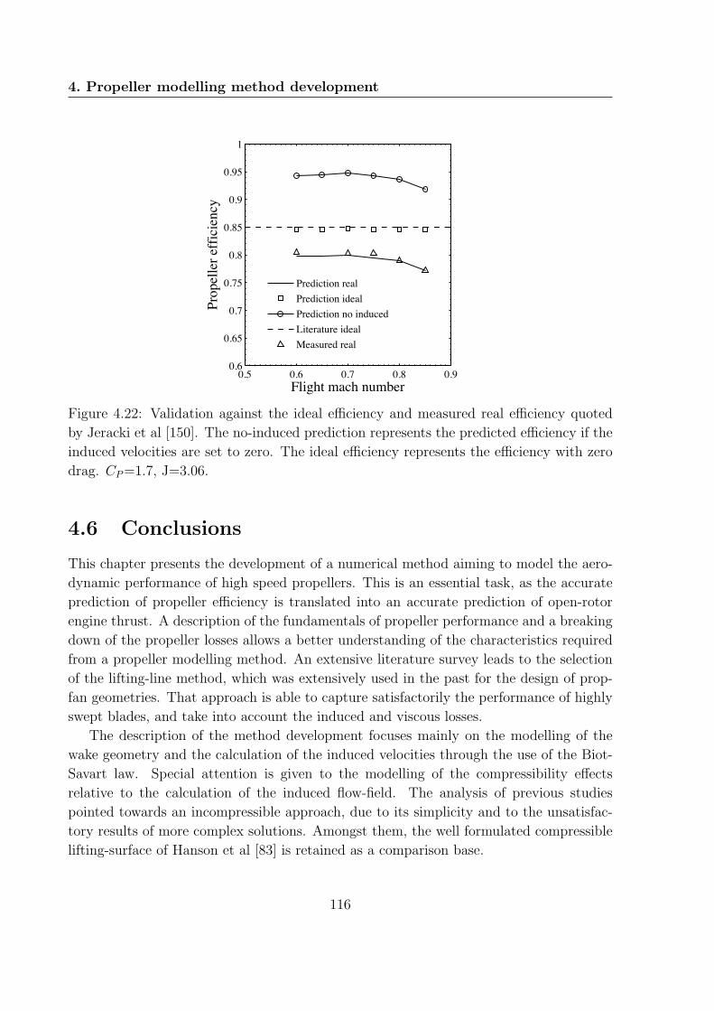
4. Propeller modelling method development

0.5 0.6 0.7 0.8 0.90.6

0.65

0.7

0.75

0.8

0.85

0.9

0.95

1

Flight mach number

Prop

elle

r effi

cien

cy

Prediction realPrediction idealPrediction no inducedLiterature idealMeasured real

Figure 4.22: Validation against the ideal efficiency and measured real efficiency quoted

by Jeracki et al [150]. The no-induced prediction represents the predicted efficiency if the

induced velocities are set to zero. The ideal efficiency represents the efficiency with zero

drag. CP=1.7, J=3.06.

4.6 Conclusions

This chapter presents the development of a numerical method aiming to model the aero-

dynamic performance of high speed propellers. This is an essential task, as the accurate

prediction of propeller efficiency is translated into an accurate prediction of open-rotor

engine thrust. A description of the fundamentals of propeller performance and a breaking

down of the propeller losses allows a better understanding of the characteristics required

from a propeller modelling method. An extensive literature survey leads to the selection

of the lifting-line method, which was extensively used in the past for the design of prop-

fan geometries. That approach is able to capture satisfactorily the performance of highly

swept blades, and take into account the induced and viscous losses.

The description of the method development focuses mainly on the modelling of the

wake geometry and the calculation of the induced velocities through the use of the Biot-

Savart law. Special attention is given to the modelling of the compressibility effects

relative to the calculation of the induced flow-field. The analysis of previous studies

pointed towards an incompressible approach, due to its simplicity and to the unsatisfac-

tory results of more complex solutions. Amongst them, the well formulated compressible

lifting-surface of Hanson et al [83] is retained as a comparison base.

116

4.6. Conclusions

The numerical method is configured in order to simulate the performance of the well-

documented SR3 prop-fan geometry, created by Hamilton Standard in 1970s. The selec-

tion of the model configuration parameters is conducted by using an extensive sensitivity

analysis. In addition to setting up the model, this analysis sheds light to many interest-

ing modelling aspects. Most notably, the results confirm the selection of the prescribed

wake model against the rigid helical one, which would lead in a severe under-prediction

of efficiency. Furthermore, the effect of blade deformations is proven to induce a reduc-

tion in the power coefficient of about 0.22, especially at high mach numbers. The nacelle

modelling using the public domain potential flow code PAN AIR, is found to predict well

the flow around the SR3 spinner and nacelle, especially in the high power blade region.

Having verified the code set-up, the modelling of deformations and the accuracy of the

nacelle prediction, the code is validated against experimental data. At low Mach number

(M=0.2) the predictions show very good agreement with the test data, both for the power

coefficient and the efficiency. At M=0.6 the agreement is still very good but the pitch

angle is under-predicted by 2 degrees due to the increased effect of the deformations.

This effect is attributed to the elastic behaviour of the blade retention system, which

was not captured by the implemented modelling. At M=0.8 the agreement is not as

good, due to the combined effect of deformations and compressibility. Nevertheless, the

prediction is in the same order of accuracy as the higher fidelity compressible lifting-surface

method of Hanson et al [83]. This result further reinforces the choice for an incompressible

calculation of the induced velocities. In an attempt to reduce the effect of deformations,

a last validation exercise is conducted with constant power coefficient and advance ratio.

This time the agreement with the experimental data is excellent throughout the whole

Mach number range, proving the suitability of the code for the performance predictions

required in the context of this work.

117

4. Propeller modelling method development

118

Chapter 5

The development of a scalable

propeller map representation

5.1 Introduction

The aim of this chapter is to devise a propeller map representation approach able to

capture the performance of different propeller designs. This can also be achieved by the

method developed in the previous chapter if the geometry of the propeller is known.

However, this is not the case during the early stages of engine parametric studies and

design space explorations. Normally at this early phase the designer has access to a limited

set of maps which correspond to specific propeller geometries. The effect of varying the

propeller design is captured by scaling and interpolating between the existing maps, with

the design space being limited by the availability of data. For the scaling to be generic,

it must be physics based and should only use global propeller design parameters that can

be available at the preliminary design phases. The generation of such a generic scaling

method is the ultimate objective of this chapter.

The chapter begins with a literature survey that details previous attempts to give a

generic propeller representation within the context of an engine design study. The lifting-

line method described in the previous chapter is used in order to produce a complete

propeller map in the conventional form described in section 4.2. At this point, the focus

turns to selecting a convenient way of capturing the effect of Mach number. Subsequently,

the propeller model is used within a sequential quadratic programming framework in order

to optimise the blade twist and chord distribution for different sets of design parameters.

A complete propeller performance map is then generated for each one of the optimised

designs. The generated maps are analysed with the sole purpose of identifying a propeller

performance representation method that is scalable between different propeller designs.

119

5. The development of a scalable propeller map representation

5.2 Propeller map scaling literature

As described in section 4.2 the traditional representation of propeller performance consists

of tables or graphs that give the efficiency or thrust coefficient as a function of advance

ratio and power coefficient. The effect of compressibility is then captured either by ad-

ditional data tables for each Mach number [79], or with a correlation which corrects the

efficiency as a function of Mach [81]. This data pack is repeated for different propeller

geometries that cover a wide range of ”prime geometry variables” as mentioned in Wain-

auski et al [79]. These variables can include the tip speed, diameter, horsepower, blade

number, integrated lift coefficient and activity factor just to mention the most important

ones. It must be noted here that the integrated lift coefficient represents the average

section design lift coefficient weighted by the radius cubed, while the activity factor is a

measure of the solidity and chord of the blade [79]. Designers can then interpolate in this

bulky set of data in order to perform trade-off studies between the different parameters

[151].

Borst [99] noted that in order to cover the necessary range, numerous maps of coherent

characteristics would be required and therefore suggested a more convenient process.

More specifically, he recommended the use of propeller theory in order to minimise the

required amount of data. In doing so, he separated the ideal and viscous losses and

modelled the blade in a simplified way by assuming that the performance at the 3/4 of

the radius represents the performance of the whole blade. This helped him understand

the different loss sources and how they change for different designs. For example, the

viscous losses are connected to the aerodynamic efficiency of the airfoil section which is

equal to CL/CD. This in turn depends on the lift coefficient CL of the section. For given

operating conditions, power can be produced either by higher lift coefficients or by higher

blade chords. This means that for a given power, the higher the blade chord the lower

the required lift coefficient [148]. Borst formulated this relationship as shown in Eq. 5.1,

where NB is the number of blades. He then used a propeller simulation code to produce

his results and populate graphs that depict this relation. These graphs were contour

plots where the x-axis was the advance ratio J (representing the operating conditions),

the y-axis the ”loading factor” CPNB ·AF

and the contours the ratio CL/CD representing the

viscous losses.

CL = f

(CP

NB · AF

)⇒ CL/CD = f

(CP

NB · AF

)(5.1)

It must be noted here that CP is the operating power coefficient and not the design

one. The design power coefficient is implicitly taken into account by the activity factor

AF ; i.e. a propeller of higher power would eventually (but not necessarily) have a higher

activity factor. Hence, the selection of the activity factor is left on the user of the method,

as according to Borst’s approach this is the parameter that distinguishes one propeller

120

5.2. Propeller map scaling literature

from the other. To summarize, by using the aforementioned graph of Eq. 5.1, the designer

can estimate the CL/CD ratio for a given number of blades, activity factor, advance ratio

and power coefficient (the last two representing the operating conditions).

After having estimated the viscous losses through the calculation of CL/CD the fi-

nal efficiency is calculated according to a second graph given by Borst. This graph uses

advance ratio, power coefficient and CL/CD as the independent variables and the pro-

peller efficiency as the dependent. More precisely, a different graph corresponds to each

value of CL/CD, and this is repeated also for different blade numbers. By this second

graphical correlation, Borst essentially adds the effect of ideal losses which only depend

on the advance ratio and power coefficient as discussed in section 4.5.3. Following Borst’s

approach a designer could model the performance of propellers of different activity factors

and different blade numbers.

However, to the best of the author’s knowledge the method has never been used in

the public domain. Some possible explanations can be given by carefully examining the

salient features of the method. First of all, the selection of the activity factor as the main

design parameter is not convenient for engine design studies. The main parameters used

interchangeably in this kind of studies is the power coefficient or the disk loading P/D2,

supplemented by the advance ratio. These parameters can readily be calculated by the

definition of macroscopic variables such as the propeller diameter, rotational speed, flight

speed and the power supplied. If one wanted to use Borst’s approach, they should be able

to relate the changes in the design power coefficient or advance ratio to the changes in

activity factor. Secondly, the method uses the aerodynamic efficiency as a parameter in

the graphs. This was possible because the graphs were populated by simulation results,

where these variables are conveniently available in the output file. However, if one wanted

to use the method in conjunction with a measured set of data, he would only have in hand

the efficiency, power/thrust coefficient and advance ratio. Thus the method would not be

applicable to maps already existing in the public domain in the aforementioned format.

Thirdly, the method does not seem to take into account the effect of flight Mach number

and the associated compressibility effects. Finally, although the number of required graphs

has been greatly reduced, the second set of graphs still requires a set of data equal to:

(number of different blade numbers) × (number of different CL/CD). Notwithstanding its

disadvantages this work was the first attempt to use a physics-based map representation

by separating the induced and viscous losses and it was one of the studies that instigated

the method presented later in this chapter.

The propeller method by S.B.A.C. [152], albeit being computational and not relevant

to map scaling, supplied useful ideas towards the development of a scalable map. This

approach consists in simple calculations conducted for the 3/4 radius point of the blade.

The method itself is not very accurate, as it is based on approximative solutions of the

Goldstein equation and on the performance of a single blade point. Nevertheless, the

121

5. The development of a scalable propeller map representation

important element is that once again the method splits the ideal and viscous efficiencies

and calculates a total efficiency as their product. This technique, together with the

selection of the 3/4 point as representative of the whole blade performance, will be retained

as useful elements for the subsequent developments.

As the open-rotor concept has been historically connected to the level of fuel prices,

there was no continuous development of the modelling methodology [79]. Nowadays, the

simulation capability is being reinvented and references [19–24] are modern studies on the

topic. Hendricks [20] implemented the open-rotor capability in the NPSS code simply by

adding a given map corresponding to a specific geometry. This method was then used

by the studies [19, 21, 24]. Seitz [22, 23] followed a more generic approach by using a

Theodorsen design code, to calculate the design point efficiency and with this scale a

given map. However, Seitz never proved the suitability of his method and the error it

introduces. It seems that the know-how and the ideas developed by Borst and S.B.A.C.

were not taken on-board by contemporary researchers. It this gap in the development of

propeller map representation methods that this chapter aims to fill.

5.3 SR3 prop-fan map

Before studying the effect of different designs, it is essential to study the variation within a

map of a given design. More specifically, the method developed in the previous chapter is

used in order to produce complete performances maps for the SR3 propeller. As shown in

Fig. 5.1a, the map is in the form of efficiency contours, with the advance ratio and power

coefficient being the independent variables and the flight Mach number being constant

(M=0.2 in this case). The iso-pitch-angle lines, which are also depicted, are not used for

the performance calculations but are useful in explaining the different phenomena taking

place.

As one observes from Fig. 5.1a, the efficiency of a constant pitch angle line increases

until an optimum is reached and then decreases. This variation can be explained by

studying the effect of advance ratio on the ideal and viscous losses. Starting from the

ideal losses, lower advance ratio means that the wake helical vortices will be closer to

the blades and therefore impact more their performance. Furthermore, a decrease in

advance ratio also leads to an increase in the power coefficient, which in turn intensifies

the strength of the trailing vortices and increases the ideal losses. Figure 5.1b depicts the

variation of ideal efficiency and confirms these arguments. It must be reminded here that

the ideal efficiency is the efficiency of the propeller calculated by setting the drag to zero.

In summary, the ideal losses increase monotonously as the advance ratio decreases. This

means that the effect of non-optimal distribution of loading reported by Mikkelson et al

[80] seems to have a negligible impact, or else a region of optimum ideal efficiency would

occur.

122

5.3. SR3 prop-fan map

1 2 3 4

0.5

1

1.5

2

2.5

Efficiency ï M=0.2

Advance ratio J

Pow

er c

oeff

icie

nt C

P 0.2

0.3

0.4

0.5

0 6

0.6

0.7

0.70.8

0.80.8340o

48o52o

56o

60o62o

(a) Efficiency

1 2 3 4

0.5

1

1.5

2

2.5

Ideal efficiency ï M=0.2

Advance ratio J

Pow

er c

oeff

icie

nt C

P

0.4

0.5

0.6

0.7

0.8

0.9

0 9

0.9540o

48o

52o56o

60o

62o

(b) Ideal efficiency

Figure 5.1: A full performance map for the SR3 propeller at low speed conditions M=0.2.

The contours represent the real or ideal efficiency, while the iso-pitch-angle lines are

depicted in dashed style.

The presence of an optimum efficiency is thus expected to be due to the viscous losses

behaviour, explained hereafter. The aforementioned increase in the power coefficient for

a decreasing advance ratio, comes about due to an increase in the angle of attack seen

by the blade elements. This results from the increased rotational speed Ω and peripheral

velocity, which rise for a decreasing advance ratio when the flight speed V0 is kept constant

(as it is fixed by the flight Mach number). The variation of the angle of attack is confirmed

by the results shown in Fig. 5.2. The points of the graph falling in the region where the

angle is higher than 8 degrees represent operating conditions where the blade stall starts

expanding and thus are less accurate. The rising angle of attack results in a variation in

the aerodynamic efficiency of the blades (L/D), which reaches an optimum value as the

angle increases and then decreases.

In addition to the angle of attack effect there is also the effect of rising compressibility

losses due to the higher Mach number seen by the airfoils for decreasing advance ratio.

This is explained clearly by examining the Eq. 5.2 that gives the definition of helical Mach

number for a given r/R ratio of the blade radius. This variable is a simple vector sum of

the axial and rotational Mach numbers and it gives an approximation of the total Mach

number seen the blade element at that radius (it is not 100% accurate, as it neglects the

effect of induced velocities and blade sweep). It is clear from Eq. 5.2 that a decrease in J

leads to a monotonous increase in Mh, which in turn aggravates the compressibility losses

and decreases the efficiency.

Thus, it can be concluded that it is the viscous losses variation that leads to the

123

5. The development of a scalable propeller map representation

1 2 3 4

0.5

1

1.5

2

2.5

Angle of attack @0.75R ï M=0.2

Advance ratio J

Pow

er c

oeffi

cien

t CP

0

24

68

1012

1416

40o48o

52o56o

60o62o

Figure 5.2: The variation of the angle of attack at the 3/4 blade radius for the SR3

propeller at low speed conditions M=0.2. The angles are in degrees, while the iso-pitch-

angle lines are depicted in dashed style.

presence of an optimum in the efficiency variation at constant pitch angle.

Mh = M ·√

1 +( rR

π

J

)2

(5.2)

The same logic applies if one tries to explain the variation of efficiency for constant

advance ratio J when the pitch angle varies. This time the wind angle of attack is fixed

by the advance ratio and the blade pitch angle is the one varying. On the other hand,

the effect of varying the advance ratio at constant CP is more complicated to explain and

the simplified blade element of Fig. 5.3 will be used as an aid. This figure represents the

performance of a simplified case, where the blade is straight, there is no drag, no induced

velocities and no effect of nacelle. Under these conditions no transformation of coordinate

systems is required and the free-stream flight speed and rotational velocity directly define

the angle of attack for a given pitch angle B.

Equation 5.3 gives the definition of the power coefficient of the element i, with the

power being replaced by the product of torque and rotational speed. Then, the torque

is replaced by the appropriate component of the element lift, which is calculated by the

definition of the lift coefficient CL as shown in Eq. 5.4. Then the angle φ and the total

velocity Vcn are calculated by the axial and rotational velocity components as shown in

Eq. 5.5. Finally, by introducing the definition of the advance ratio J (Eq. 4.3) and after

some algebraic manipulations, Eq. 5.6 is derived.

124

5.3. SR3 prop-fan map

c n

s

V cn α

L

α B

φ

Ωr

V0

Z Y

X

φ

T

Qr

Figure 5.3: Simplified blade element performance. The schematic assumes a straight

blade with zero induced velocities, zero drag and no effect of nacelle.

CP,(i) =P(i)

ρ · n3 ·D5=

Ω ·Q(i)

ρ · n3 ·D5(5.3)

CP,(i) =Ω

ρ · n3 ·D5· 1

2ρc(i)CL,(i) · V 2

cn,(i) · sinφ(i) · r(i) (5.4)

CP,(i) =Ω

ρ · n3 ·D5· 1

2ρc(i)CL,(i)

[V 2

0 +(Ωr(i)

)2] · sin [tan−1

(V0

Ωr(i)

)]· r(i) (5.5)

CP,(i) =πMc(i)V

20

D3· CL,(i) · sin

[tan−1

(J

r(i)Rπ

)]·[1 +

(r(i)R

π

J

)2]· r(i) (5.6)

The first term of Eq. 5.6 is constant, the second is the lift coefficient CL and the

terms three and four depend on the advance ratio. More specifically, term three increases

with increasing advance ratio, while term four decreases. Amongst them, term three

is more powerful and dominates. Thus the ensemble of terms three and four increases

with advance ratio. This means that for a constant power coefficient, when the advance

ratio increases, the increase of the advance ratio term will need to be compensated by

a corresponding decrease of the lift coefficient. This is confirmed by Fig. 5.2 which

shows that for constant power coefficient, the angle of attack falls when the advance ratio

increases. At the same time the pitch angle increases in order to follow the blade element

φ angle increase. More precisely, the increase of advance ratio leads to a decrease in the

Ωr velocity component and a corresponding increase in the angle φ, as shown in Fig. 5.3.

For a constant angle of attack this would lead to a parallel increase of the pitch angle; i.e.

125

5. The development of a scalable propeller map representation

the increasing φ would ”push” the pitch angle B towards the axial direction. In this case

the angle of attack decreases, a fact which slightly abates the increasing pitch effect.

Finally, Fig. 5.4 shows an alternative representation of performance using the thrust

coefficient CT in the place of efficiency. As seen in the figure, the variation of CT is more

”linear” and therefore more adapted for computerisation and interpolation. However,

within the context of this chapter the efficiency map is preferred as it facilitates the

explanation of the different phenomena.

1 2 3 4

0.5

1

1.5

2

2.5

Thrust coefficient ï M=0.2

Advance ratio J

Pow

er c

oeffi

cien

t CP

0.1

0.2

0.3

0.4

0.5

0.60.7

0.8

40o48o

52o56o

60o62o

Figure 5.4: An alternative CT performance map for the SR3 propeller at low speed condi-

tions M=0.2. The contours represent the thrust coefficient, while the iso-pitch-angle lines

are depicted in dashed style.

5.3.1 The Mach number effect

Having established the performance representation for a single flight Mach number, the

next step is to investigate the effect of different flight speeds. This has been traditionally

taken into account either by multiple maps, one for each Mach, or by using a correlation

that corrects the efficiency in function with the Mach number. The first solution offers

potentially higher accuracy at the cost of larger data tables, while the second offers the

opposite. However, the difference in accuracy between the two methods has never been

tested before.

Figures 5.5a and 5.5b show the efficiency map of the SR3 propeller for Mach numbers

equal to 0.6 and 0.8 respectively. The comparison between these maps and the one shown

earlier in Fig. 5.1a illustrates that the efficiency contours are compressed towards the high

advance ratio region. This means that the efficiency in the lower advance ratio region gets

126

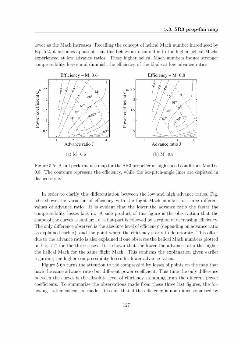
5.3. SR3 prop-fan map

lower as the Mach increases. Recalling the concept of helical Mach number introduced by

Eq. 5.2, it becomes apparent that this behaviour occurs due to the higher helical Machs

experienced at low advance ratios. These higher helical Mach numbers induce stronger

compressibility losses and diminish the efficiency of the blade at low advance ratios.

1 2 3 4

0.5

1

1.5

2

2.5

Efficiency ï M=0.6

Advance ratio J

Pow

er c

oeff

icie

nt C

P 0.4

0.5

0.6

0.7

0.8

0.825

0.7

48o52o

56o

60o62o

(a) M=0.6

1 2 3 4

0.5

1

1.5

2

2.5

Efficiency ï M=0.8

Advance ratio J

Pow

er c

oeff

icie

nt C

P

0.4

0.5

0.6

0.7

0.8

0.82550o

54o

58o

61o

(b) M=0.8

Figure 5.5: A full performance map for the SR3 propeller at high speed conditions M=0.6-

0.8. The contours represent the efficiency, while the iso-pitch-angle lines are depicted in

dashed style.

In order to clarify this differentiation between the low and high advance ratios, Fig.

5.6a shows the variation of efficiency with the flight Mach number for three different

values of advance ratio. It is evident that the lower the advance ratio the faster the

compressibility losses kick in. A side product of this figure is the observation that the

shape of the curves is similar; i.e. a flat part is followed by a region of decreasing efficiency.

The only difference observed is the absolute level of efficiency (depending on advance ratio

as explained earlier), and the point where the efficiency starts to deteriorate. This offset

due to the advance ratio is also explained if one observes the helical Mach numbers plotted

in Fig. 5.7 for the three cases. It is shown that the lower the advance ratio the higher

the helical Mach for the same flight Mach. This confirms the explanation given earlier

regarding the higher compressibility losses for lower advance ratios.

Figure 5.6b turns the attention to the compressibility losses of points on the map that

have the same advance ratio but different power coefficient. This time the only difference

between the curves is the absolute level of efficiency stemming from the different power

coefficients. To summarize the observations made from these three last figures, the fol-

lowing statement can be made. It seems that if the efficiency is non-dimensionalised by

127

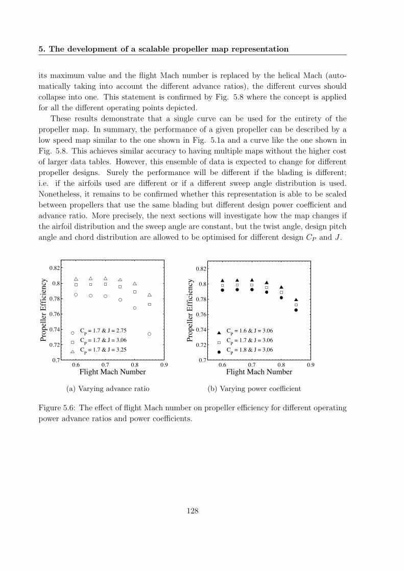
5. The development of a scalable propeller map representation

its maximum value and the flight Mach number is replaced by the helical Mach (auto-

matically taking into account the different advance ratios), the different curves should

collapse into one. This statement is confirmed by Fig. 5.8 where the concept is applied

for all the different operating points depicted.

These results demonstrate that a single curve can be used for the entirety of the

propeller map. In summary, the performance of a given propeller can be described by a

low speed map similar to the one shown in Fig. 5.1a and a curve like the one shown in

Fig. 5.8. This achieves similar accuracy to having multiple maps without the higher cost

of larger data tables. However, this ensemble of data is expected to change for different

propeller designs. Surely the performance will be different if the blading is different;

i.e. if the airfoils used are different or if a different sweep angle distribution is used.

Nonetheless, it remains to be confirmed whether this representation is able to be scaled

between propellers that use the same blading but different design power coefficient and

advance ratio. More precisely, the next sections will investigate how the map changes if

the airfoil distribution and the sweep angle are constant, but the twist angle, design pitch

angle and chord distribution are allowed to be optimised for different design CP and J .

0.6 0.7 0.8 0.90.7

0.72

0.74

0.76

0.78

0.8

0.82

Flight Mach Number

Prop

elle

r Effi

cien

cy

CP = 1.7 & J = 2.75CP = 1.7 & J = 3.06CP = 1.7 & J = 3.25

(a) Varying advance ratio

0.6 0.7 0.8 0.90.7

0.72

0.74

0.76

0.78

0.8

0.82

Flight Mach Number

Prop

elle

r Effi

cien

cy

CP = 1.6 & J = 3.06CP = 1.7 & J = 3.06CP = 1.8 & J = 3.06

(b) Varying power coefficient

Figure 5.6: The effect of flight Mach number on propeller efficiency for different operating

power advance ratios and power coefficients.

128

5.3. SR3 prop-fan map

0.6 0.7 0.8 0.9 10.5

0.6

0.7

0.8

0.9

1

1.1

Flight Mach Number

Hel

ical

Mac

h N

umbe

r @0.

75R

CP = 1.7 & J = 2.75CP = 1.7 & J = 3.06CP = 1.7 & J = 3.25

Figure 5.7: The variation of helical mach number at the 3/4 of the blade radius for

different flight mach numbers and advance ratios.

0.6 0.8 1 1.2

0.85

0.9

0.95

1

Helical Mach Number @0.75R

Rela

tive

Prop

elle

r Effi

cien

cy

CP = 1.7 & J = 3.06CP = 1.7 & J = 3.25CP = 1.7 & J = 2.75CP = 1.6 & J = 3.06CP = 1.8 & J = 3.06

Figure 5.8: The variation of relative efficiency with helical mach number at 0.75R for

different operating advance ratios and power coefficients. The relative efficiency is defined

as the efficiency divided by the maximum efficiency for a given advance ratio and power

coefficient.

129

5. The development of a scalable propeller map representation

5.4 Design and optimisation

5.4.1 The propeller design problem

Before starting the propeller design exercise, the design problem must first be briefly de-

scribed. That is the problem of selecting all the parameters that define the geometry of

the propeller, as described by numerous studies conducted by Hamilton Standard and

NASA [82, 104, 112, 148, 150]. To begin with, the number of blades is normally selected

as high as possible in order to minimise the ideal losses. However, after a certain number

the blades encounter an efficiency loss due to choking at the propeller hub [112]. Further-

more, a higher number of blades is also translated in a higher propeller weight and cost.

The thickness to chord ratio of the airfoils is normally selected as the lowest allowed by

the stress limits, aeroelastic response considerations and fabrication state-of-the-art [82].

According to Stefko and Jeracki [148] the design lift coefficient of the airfoils is selected

in a way that maximises the aerodynamic efficiency for a given power and minimises the

drag. Finally, the selection of the sweep angle distribution aims to achieve subcritical

Mach numbers along the blade and reduce the compressibility losses [104]. However, dur-

ing the design of the SR3 prop-fan the sweep was varied in a way that reduces the emitted

noise [101].

All the aforementioned design parameters belong to the sphere of propeller design

and fall outside the context of this work. In the context of whole engine design, this

work focuses only on the variation of macroscopic design parameters. These macroscopic

parameters are the design power coefficient and design advance ratio, which are directly

related to the power, shaft speed, diameter restriction and flight speed of the engine.

For each set of macroscopic design parameters the propeller performance is optimised

by selecting the values of the propeller twist angle and chord distribution. The twist

distribution is mainly connected to the ideal performance, whilst the chord distribution

affects the viscous drag losses [106]. The blade characteristics described in the previous

paragraph are considered constant and related to the specific propeller design.

In summary, within the context of this chapter a propeller of given blading is taken and

its design power coefficient and advance ratio are varied. The twist and chord distributions

are redesigned in order to minimise the ideal and viscous losses for the new propeller.

The new propeller geometry is used in order to generate a complete performance map

and study how this has changed relative to the baseline design.

5.4.2 Method selection

There are two main approaches to conduct the propeller design exercise. The first is the

fastest but more old fashioned, as it is based on the theories of Goldstein and Theodorsen.

This approach has been used in the studies by Davidson [109], McKay [108] and Adkins

130

5.4. Design and optimisation

et al. [106]. The method is based on the optimality condition first stated by Betz [92] and

subsequently used by Goldstein [97], which says that an ideal propeller generates a wake

of rigid helical shape. As described by Wald [84], this rigid wake requires a constant wake

displacement velocity, which is the only unknown variable in the optimisation problem (at

least at its simplest version). The wake displacement velocity is the velocity with which

the rigid helix travels backwards. This variable, coupled with a specified lift coefficient

distribution, is iterated in order to match a specified design power coefficient. After

the power coefficient is matched, the method gives automatically the twist and chord

distribution. The distribution of lift coefficient should be chosen in a way that optimises

the L/D at each airfoil station. The method gives a clear vision of the physics involved

and more specifically, it shows the independence between the optimisation of the ideal

losses and the viscous losses. This fact was also described by Adkins et al. [106] and

by Borst [99], who reported that the ideal losses are minimised through the selection of

twist, while the viscous losses via the selection of the chord or L/D of each section.

Although this method is extremely fast (it takes less than a few seconds), it inherits

all the shortcomings of the Goldstein approach. The greatest among them, it cannot

handle correctly swept blades. Mikkelson et al. [80] mentioned this problem for the swept

SR1 propeller, which was designed using a Goldstein approach. According to them, the

designed twist resulted in a non-optimal loading distribution and the blade needed to be

retwisted. They finally had to turn to a lifting-line method, similar to the one developed

in the previous chapter. The transition to lifting-line methods comes at the cost of higher

computational requirements. The method is not able to ”reverse engineer” the optimum

distribution of twist and chord by imposing a rigid wake and an optimisation method is

required.

Chang and Sullivan [153] chose a gradient based penalty method to translate the

constrained optimisation problem to a sequence of corresponding unconstrained ones.

This optimisation method adds a penalty term to the objective function that corresponds

to the violation of the constraint specified. At each different step of the solution the weight

of the penalty term is increased and in the end the unconstrained problem converges

towards the constrained. Chang and Sullivan used this method to optimise the twist of a

swept blade for a given pitch angle, under the constraint of a specified power coefficient.

The authors also proved that their approach is consistent with the traditional Goldstein

method when the propeller blades are straight.

Cho and Lee [154] used a gradient based optimisation technique similar to the one

of Chang and Sullivan [153], which was once more coupled with a lifting-line code. In

addition to optimising the twist they also calculated the optimal distribution of chord.

Interestingly, they did the optimisation in two steps: first they optimised the twist and

then the chord. Although the authors did not comment on this choice, it can be assumed

that it is due to the independence of the two figures of merit; i.e. the ideal and viscous

131

5. The development of a scalable propeller map representation

losses. Another interesting finding of their work concerns the selection of the number

of blade elements. They reported that around 10 elements are enough for the result to

converge to an optimum, while more elements would increase the numerical difficulty of

the problem and they could also result in a ”wiggly” variation of twist and chord.

Gur and Rosen [93] proposed a combination of three optimisation methods in order

to achieve a high optimisation robustness and also produce a smooth variation of twist

and chord. In the first stage a genetic algorithm was used in order to bring the solution

closer to the global optimum. The authors argued that this algorithm could not handle

well multiple constraints and also produced non-smooth results. Thus, they decided to

add a linear simplex method at the second stage. This time, the smoothness of the design

variation was achieved by constraining the second derivative of twist and chord at each

blade element. The smoother result of the simplex method was finally input to a gradient

based method which climbed the rest of the hill to reach the optimum value. As with

the two previous cases, Gur and Rosen also used penalty functions, but contrary to the

others based their predictions to a simpler blade-element/momentum propeller model.

However, it has to be noted that they limited their study to low speed straight blades.

The use of three consecutive optimisation techniques was justified due to the high number

of variables used in this study, which optimised in parallel the aerodynamics, acoustics

and structural integrity. Within this chapter, the optimisation problem is limited to the

aerodynamic design of twist and chord and thus such a hybrid scheme would lead to

unnecessary excessive evaluations.

The design method chosen for this work follows the approach of references [153] and

[154], by coupling the developed lifting-line method with a gradient based optimiser. More

specifically the author chose the Sequential Quadratic Programming method available in

the non-linear optimisation toolkit of the Matlab platform. This approach was preferred

to the classic Goldstein one, firstly because it can take advantage of the higher fidelity

lifting-line method and secondly because in future developments it could also incorporate

disciplines other than aerodynamics, as done by Gur and Rosen [93].

5.4.3 Optimisation problem formulation

According to what was discussed in sections 5.4.1 and 5.4.2, the optimisation problem

can be stated as follows. For a given blade geometry, optimise the pitch angle and the

twist/chord distributions in order to achieve optimum propeller efficiency for a given flight

Mach number, advance ratio and power coefficient. As discussed in section 5.4.1 the rest

of the blade characteristics falls in the domain of hardcore propeller design and are not

relevant to the global performance investigations of this work.

The given blade geometry includes:

• the number of blades

132

5.4. Design and optimisation

• the blade hub to tip ratio

• the sweep angle distribution

• the selection of airfoils

The non-linear optimisation problem is thus formulated as:

Maximise the objective function

ηprop(B, ~∆β,~c) (5.7)

Subject to the constraints

CP ( ~B,∆β,~c)− CP,des = 0

0 ≤ B ≤ 90

−45 ≤ ∆βi ≤ +45, i = 1..(N + 1)

0 ≤ ci ≤ R, i = 1..(N + 1)

∣∣∣∣d2(∆βi)

dr2

∣∣∣∣ ≤ C1, i = 1..(N − 1)

∣∣∣∣d2(ci)

dr2

∣∣∣∣ ≤ C2, i = 1..(N − 1)

Where B is the blade pitch angle, ~∆β = [∆β1,∆β2, ...∆βN+1]T the design vector of

twist, ~c = [c1, c2, ...cN+1]T the design vector of chord, r the local blade radius, R the blade

tip radius and N is the number of blade elements (it is reminded that N blade elements

are bounded by N + 1 blade geometry points). The advance ratio J is an input of the

lifting-line method, while the power coefficient CP is an output and hence it has to be

added as an equality constraint. The constraints in the second derivatives ensure a smooth

variation of the twist and chord of the blade, as done by Gur and Rosen [93]. Experience

with the model showed that the values of C1 = 100 and C2 = 3 give satisfactory results.

In order to isolate the different effects and especially the ideal and viscous losses,

the optimisation exercise will be carried out in two phases. In the first phase only the

twist and pitch will be optimised, which are expected to have an impact only in the ideal

performance. This phase corresponds to the work carried out by Chang and Sullivan

[153], who only optimised the ideal efficiency. The second phase also adds the chord

133

5. The development of a scalable propeller map representation

distribution in the set of variables and solves the entirety of the design problem. This

stepped approach is expected to give a better visibility and insight into the phenomena

taking place. The results of the two steps are given in the next sections.

5.4.4 Optimisation results

The baseline geometry is that of the SR3 prop-fan as described in section 4.5.1. Following

the recommendation of Cho and Lee [154] the twist and chord are optimised for 10 blade

points (which define 9 blade elements). The effect of the nacelle is deactivated in order

to speed up the optimisation process, with no important effect on the final conclusions of

the study. Following a common practice of propeller design, the twist at the 0.75 blade

radius is set equal to zero. In order to do that, the pitch angle is ”freed” to accommodate

any variation of power, instead of varying uniformly the twist of all the blade stations.

Had the blade been straight, this would not be required as the pitch would simply be set

equal to the final optimal twist angle at the 0.75 blade radius. This angle would then be

set as the design pitch and subsequently be subtracted from all the blade station twists,

setting the angle at 0.75R automatically to zero.

5.4.4.1 Step 1: optimise twist and pitch with constant chord

As mentioned earlier during the first step of the study the chord distribution is kept the

same to the baseline blade. The five cases optimised are shown in the table 5.1. The

design Mach number for all the cases is equal to 0.8. The power coefficient CP and the

advance ratio J represent the chosen design conditions for each case, while the pitch is

the result of the optimisation process. The first observation is that the pitch increases

for increasing CP or increasing J . These trends will be more easily explained by first

examining the variation of optimal twist in Fig. 5.9 for different design advance ratios. It

is seen that there is no significant variation of the twist distribution, especially at the more

important outboard blade region. The same trend is identified for different design power

coefficients, although not shown here. This essentially means that the blade geometry is

the same for the different design conditions, the chord distribution also being constant.

The geometry being constant, the propeller just has to change its operating point on

the map. Therefore, for this case the explanations for the variations in performance have

already been given in section 5.3. An increase in CP under constant J leads to an increase

in the pitch angle and a parallel increase in the lift coefficient as shown by Fig. 5.10a.

This means that the increase in the power has to be achieved by an increase in the lift

coefficient as the chord of the blade cannot change. On the other hand, an increase in the

design advance ratio leads to a decrease of the lift coefficient as proven by Eq. 5.6 and

shown in Fig. 5.10b. As explained in section 5.3, the increase in advance ratio aligns the

velocity component closer to the axial direction, while the increase in the lift coefficient

134

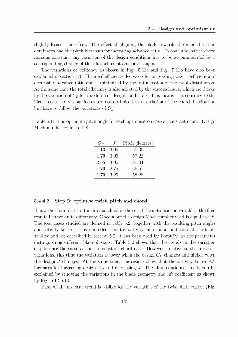
5.4. Design and optimisation

slightly lessens the effect. The effect of aligning the blade towards the axial direction

dominates and the pitch increases for increasing advance ratio. To conclude, as the chord

remains constant, any variation of the design conditions has to be accommodated by a

corresponding change of the lift coefficient and pitch angle.

The variations of efficiency as shown in Fig. 5.11a and Fig. 5.11b have also been

explained in section 5.3. The ideal efficiency decreases for increasing power coefficient and

decreasing advance ratio and is minimized by the optimisation of the twist distribution.

At the same time the total efficiency is also affected by the viscous losses, which are driven

by the variation of CL for the different design conditions. This means that contrary to the

ideal losses, the viscous losses are not optimised by a variation of the chord distribution

but have to follow the variations of CL.

Table 5.1: The optimum pitch angle for each optimisation case at constant chord. Design

Mach number equal to 0.8.

CP J Pitch [degrees]

1.13 3.06 55.36

1.70 3.06 57.22

2.55 3.06 61.04

1.70 2.75 55.57

1.70 3.25 58.26

5.4.4.2 Step 2: optimise twist, pitch and chord

If now the chord distribution is also added in the set of the optimisation variables, the final

results behave quite differently. Once more the design Mach number used is equal to 0.8.

The four cases studied are defined in table 5.2, together with the resulting pitch angles

and activity factors. It is reminded that the activity factor is an indicator of the blade

solidity and, as described in section 5.2, it has been used by Borst[99] as the parameter

distinguishing different blade designs. Table 5.2 shows that the trends in the variation

of pitch are the same as for the constant chord case. However, relative to the previous

variations, this time the variation is lower when the design CP changes and higher when

the design J changes. At the same time, the results show that the activity factor AF

increases for increasing design CP and decreasing J . The aforementioned trends can be

explained by studying the variations in the blade geometry and lift coefficient as shown

by Fig. 5.12-5.13.

First of all, no clear trend is visible for the variation of the twist distribution (Fig.

135

5. The development of a scalable propeller map representation

0.2 0.4 0.6 0.8 1ï30

ï20

ï10

0

10

20

30

Relative radius r/R

Twist

[deg

rees

]

CP = 1.7 & J = 2.75CP = 1.7 & J = 3.06CP = 1.7 & J = 3.25

Figure 5.9: The optimum distribution of twist for different design advance ratios J . The

blade chord distribution is held constant. Design Mach number equal to 0.8.

0 0.2 0.4 0.6 0.8 10

0.2

0.4

0.6

0.8

1

1.2

1.4

Relative radius r/R

Lift

coef

ficie

nt C

L

CP = 1.13 & J = 3.06CP = 1.70 & J = 3.06CP = 2.55 & J = 3.06

(a) Varying design power coefficients CP

0 0.2 0.4 0.6 0.8 10.1

0.2

0.3

0.4

0.5

0.6

0.7

0.8

Relative radius r/R

Lift

coef

ficie

nt C

L

CP = 1.7 & J = 2.75

CP = 1.7 & J = 3.06

CP = 1.7 & J = 3.25

(b) Varying design advance ratio J

Figure 5.10: The change in the lift coefficient distribution for different design power

coefficients CP and advance ratios J . The blade chord distribution is held constant.

Design Mach number equal to 0.8.

136

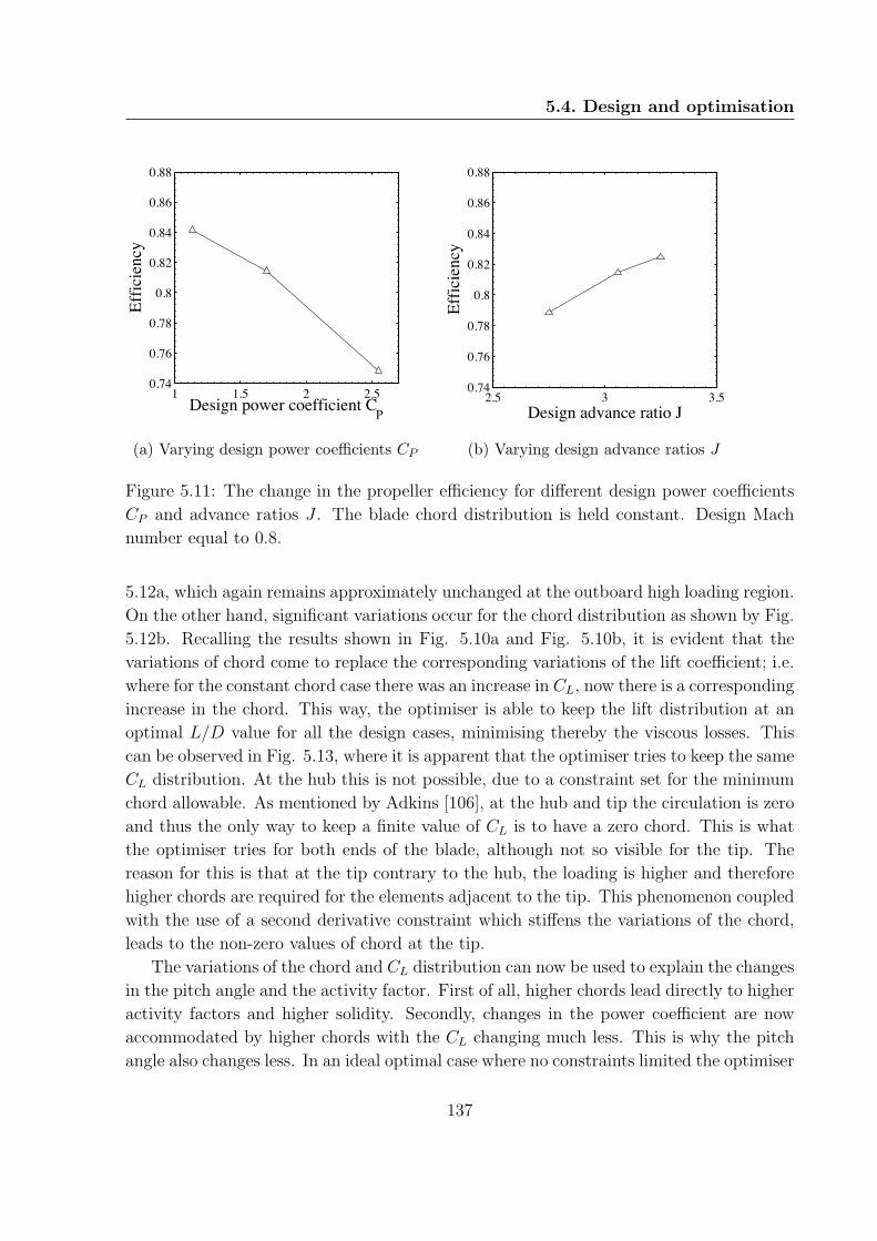
5.4. Design and optimisation

1 1.5 2 2.50.74

0.76

0.78

0.8

0.82

0.84

0.86

0.88

Design power coefficient CP

Effic

ienc

y

(a) Varying design power coefficients CP

2.5 3 3.50.74

0.76

0.78

0.8

0.82

0.84

0.86

0.88

Design advance ratio J

Effic

ienc

y(b) Varying design advance ratios J

Figure 5.11: The change in the propeller efficiency for different design power coefficients

CP and advance ratios J . The blade chord distribution is held constant. Design Mach

number equal to 0.8.

5.12a, which again remains approximately unchanged at the outboard high loading region.

On the other hand, significant variations occur for the chord distribution as shown by Fig.

5.12b. Recalling the results shown in Fig. 5.10a and Fig. 5.10b, it is evident that the

variations of chord come to replace the corresponding variations of the lift coefficient; i.e.

where for the constant chord case there was an increase in CL, now there is a corresponding

increase in the chord. This way, the optimiser is able to keep the lift distribution at an

optimal L/D value for all the design cases, minimising thereby the viscous losses. This

can be observed in Fig. 5.13, where it is apparent that the optimiser tries to keep the same

CL distribution. At the hub this is not possible, due to a constraint set for the minimum

chord allowable. As mentioned by Adkins [106], at the hub and tip the circulation is zero

and thus the only way to keep a finite value of CL is to have a zero chord. This is what

the optimiser tries for both ends of the blade, although not so visible for the tip. The

reason for this is that at the tip contrary to the hub, the loading is higher and therefore

higher chords are required for the elements adjacent to the tip. This phenomenon coupled

with the use of a second derivative constraint which stiffens the variations of the chord,

leads to the non-zero values of chord at the tip.

The variations of the chord and CL distribution can now be used to explain the changes

in the pitch angle and the activity factor. First of all, higher chords lead directly to higher

activity factors and higher solidity. Secondly, changes in the power coefficient are now

accommodated by higher chords with the CL changing much less. This is why the pitch

angle also changes less. In an ideal optimal case where no constraints limited the optimiser

137

5. The development of a scalable propeller map representation

and the CL was exactly constant, the pitch would be expected to also remain constant.

Regarding the variation of design advance ratio, the changes are more pronounced relative

to the constant chord case, as seen from tables 5.1 and 5.2. It was explained in the previous

section that there are two effects that contribute to the change of the pitch angle. The

one is the aligning of the blade towards the axial direction as the advance ratio increases

and the other is the parallel decrease in the angle of attack, which has an opposing but

lesser impact. Figure 5.13 proved that the lift coefficient and thus the angle of attack are

kept approximately constant for the optimal chord case. Therefore, the second abating

factor affecting the pitch angle, is eliminated and the variation of pitch becomes more

pronounced.

Figures 5.14a and 5.14b show the variation of efficiency for different design CP and J ,

in relation to the constant chord results showed in the previous section. It can be seen

that the trends are the same as before, but this time the efficiencies are higher. This is

normal, as this time the optimiser also minimises the viscous losses. Finally, it can be

seen from Fig. 5.14a that the initial chord distribution was closer to the optimal for the

CP = 1.7, J = 3.06 case, and that is why the distance between the constant chord and

the optimal chord efficiencies is the lowest.

Table 5.2: The optimum pitch angle for each optimisation case when the chord distribu-

tion is also optimised. Design Mach number equal to 0.8.

CP J Pitch [degrees] AF

1.13 3.06 56.24 178

1.70 3.06 57.00 271

2.55 3.06 59.16 439

1.70 2.75 54.66 326

5.5 Results analysis to devise a map scaling tech-

nique

Having optimised the blade for the different design cases, the next step consists in gener-

ating a propeller map for each one of them. The produced maps will then be analysed in

order to identify how they change according to the design. To be consistent with the maps

produced earlier for the baseline SR3 prop-fan, the effect of the nacelle will be reactivated.

The maps will be produced for the low speed Mach number of 0.2 and the effect of Mach

will be studied in a separate section. It must be noted here that in order to facilitate the

138

5.5. Results analysis to devise a map scaling technique

0 0.2 0.4 0.6 0.8 1ï40

ï30

ï20

ï10

0

10

20

30

Relative radius r/R

Twis

t [de

gree

s]

CP = 1.70 & J = 2.75CP = 1.13 & J = 3.06CP = 1.70 & J = 3.06CP = 2.55 & J = 3.06

(a) Twist

0.2 0.4 0.6 0.8 1ï0.2

ï0.1

0

0.1

0.2

0.3

Relative radius r/RC

hord

/Dia

met

er

CP = 1.70 & J = 2.75

CP = 1.13 & J = 3.06

CP = 1.70 & J = 3.06

CP = 2.55 & J = 3.06

(b) Chord

Figure 5.12: The optimum distribution of twist and chord for different design CP and J .

The blade chord distribution is optimised. Design Mach number equal to 0.8.

0.2 0.4 0.6 0.8 1 1.2

0.4

0.5

0.6

0.7

0.8

Relative radius r/R

Lift

coef

ficie

nt C

L

CP = 1.70 & J = 2.75

CP = 1.13 & J = 3.06

CP = 1.70 & J = 3.06

CP = 2.55 & J = 3.06

Figure 5.13: The change in the lift coefficient distribution for different design CP and J .

The blade chord distribution is optimised. Design Mach number equal to 0.8.

139

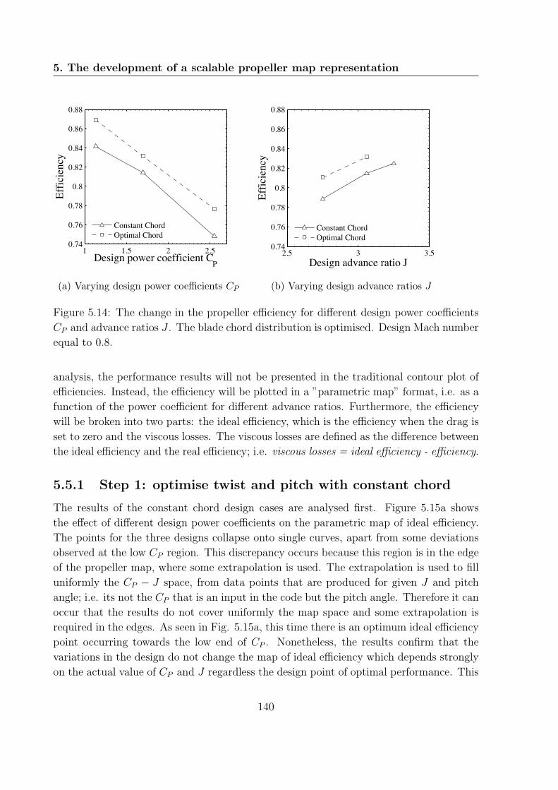
5. The development of a scalable propeller map representation

1 1.5 2 2.50.74

0.76

0.78

0.8

0.82

0.84

0.86

0.88

Design power coefficient CP

Effic

ienc

y

Constant ChordOptimal Chord

(a) Varying design power coefficients CP

2.5 3 3.50.74

0.76

0.78

0.8

0.82

0.84

0.86

0.88

Design advance ratio JEf

ficie

ncy

Constant ChordOptimal Chord

(b) Varying design advance ratios J

Figure 5.14: The change in the propeller efficiency for different design power coefficients

CP and advance ratios J . The blade chord distribution is optimised. Design Mach number

equal to 0.8.

analysis, the performance results will not be presented in the traditional contour plot of

efficiencies. Instead, the efficiency will be plotted in a ”parametric map” format, i.e. as a

function of the power coefficient for different advance ratios. Furthermore, the efficiency

will be broken into two parts: the ideal efficiency, which is the efficiency when the drag is

set to zero and the viscous losses. The viscous losses are defined as the difference between

the ideal efficiency and the real efficiency; i.e. viscous losses = ideal efficiency - efficiency.

5.5.1 Step 1: optimise twist and pitch with constant chord

The results of the constant chord design cases are analysed first. Figure 5.15a shows

the effect of different design power coefficients on the parametric map of ideal efficiency.

The points for the three designs collapse onto single curves, apart from some deviations

observed at the low CP region. This discrepancy occurs because this region is in the edge

of the propeller map, where some extrapolation is used. The extrapolation is used to fill

uniformly the CP − J space, from data points that are produced for given J and pitch

angle; i.e. its not the CP that is an input in the code but the pitch angle. Therefore it can

occur that the results do not cover uniformly the map space and some extrapolation is

required in the edges. As seen in Fig. 5.15a, this time there is an optimum ideal efficiency

point occurring towards the low end of CP . Nonetheless, the results confirm that the

variations in the design do not change the map of ideal efficiency which depends strongly

on the actual value of CP and J regardless the design point of optimal performance. This

140

5.5. Results analysis to devise a map scaling technique

result comes to confirm the observation made in section 5.3 regarding the ideal efficiency

map as shown in Fig. 5.1b.

Having in mind that the chord was kept constant and the viscous losses where not

re-optimised for each design, the results shown in Fig. 5.15b are not unexpected. The

variation of viscous losses in the parametric map is the same for all three designs. Only

the operating point of the propeller changes, with the losses being increased or decreased

according to the location of the new point on the map. This is also justified if one recalls

that the three optimised designs have the same chord and approximately the same twist

distributions. Hence, they are essentially the same blade operating at a different point.

The efficiency parametric map of Fig. 5.16a concludes this argument by showing the same

exactly performance variation for the three design CP , while Fig. 5.16b proves that the

same applies for different design advance ratios J .

0

0.5

1

J=1.15

0

0.5

1

Idea

l Effi

cien

cy

J=2.29

0 1 2 3 40

0.5

1

J=3.59

Power Coefficient CP

1.13 1.70 2.55

Design CP

(a) Ideal efficiency

0

0.2

0.4J=1.15

0

0.2

0.4

Visc

ous l

osse

s

J=2.29

0 1 2 3 40

0.2

0.4J=3.59

Power Coefficient CP

1.13 1.70 2.55Design CP

(b) Viscous losses

Figure 5.15: The change in the ideal efficiency and viscous losses map for different design

power coefficients CP . The blade chord distribution is held constant. Mach = 0.2.

5.5.2 Step 2: optimise twist, pitch and chord

The next step consists in analysing the map generated for propellers of which the distribu-

tion of chord has also been optimised. Figure 5.17a shows that the ideal efficiency is still

unaffected. There is a slight divergence of the points for low CP and for high CP at the

lowest advance ratio. Once more the explanation can be sought in the extrapolation tak-

ing place in these regions, as mentioned earlier. Furthermore, this graph is another proof

141

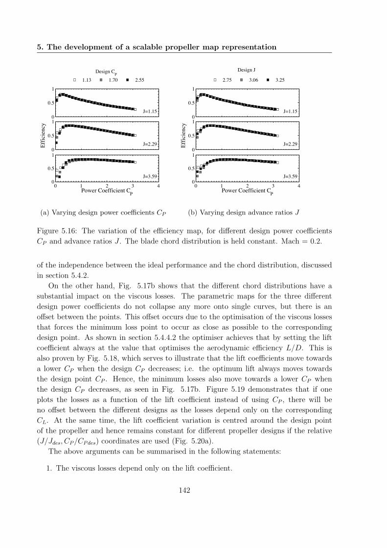
5. The development of a scalable propeller map representation

0

0.5

1

J=1.15

0

0.5

1

Effic

ienc

y

J=2.29

0 1 2 3 40

0.5

1

J=3.59

Power Coefficient CP

1.13 1.70 2.55Design CP

(a) Varying design power coefficients CP

0

0.5

1

J=1.15

0

0.5

1

Effic

ienc

y

J=2.29

0 1 2 3 40

0.5

1

J=3.59

Power Coefficient CP

2.75 3.06 3.25

Design J

(b) Varying design advance ratios J

Figure 5.16: The variation of the efficiency map, for different design power coefficients

CP and advance ratios J . The blade chord distribution is held constant. Mach = 0.2.

of the independence between the ideal performance and the chord distribution, discussed

in section 5.4.2.

On the other hand, Fig. 5.17b shows that the different chord distributions have a

substantial impact on the viscous losses. The parametric maps for the three different

design power coefficients do not collapse any more onto single curves, but there is an

offset between the points. This offset occurs due to the optimisation of the viscous losses

that forces the minimum loss point to occur as close as possible to the corresponding

design point. As shown in section 5.4.4.2 the optimiser achieves that by setting the lift

coefficient always at the value that optimises the aerodynamic efficiency L/D. This is

also proven by Fig. 5.18, which serves to illustrate that the lift coefficients move towards

a lower CP when the design CP decreases; i.e. the optimum lift always moves towards

the design point CP . Hence, the minimum losses also move towards a lower CP when

the design CP decreases, as seen in Fig. 5.17b. Figure 5.19 demonstrates that if one

plots the losses as a function of the lift coefficient instead of using CP , there will be

no offset between the different designs as the losses depend only on the corresponding

CL. At the same time, the lift coefficient variation is centred around the design point

of the propeller and hence remains constant for different propeller designs if the relative

(J/Jdes, CP/CPdes) coordinates are used (Fig. 5.20a).

The above arguments can be summarised in the following statements:

1. The viscous losses depend only on the lift coefficient.

142

5.5. Results analysis to devise a map scaling technique

2. The lift coefficient is always at the optimal value at the design point.

3. Hence the minimum losses will always move to the design point.

Therefore, if the coordinates of the viscous losses map are non-dimensionalised by

dividing them with their design values, the viscous losses will always stay constant and

centred at the point J/Jdes = 1 and CP/CPdes = 1. This is illustrated by Fig. 5.20b,

where the relative CP is used and all the points collapse onto single curves. Although not

shown here, the same principle applies for different design advance ratios according to the

analysis in section 5.4.4.2.

In conclusion, a propeller of whichever design power coefficient and advance ratio,

which is based on the same blading characteristics, can be described by a single set of two

maps. One that describes the variation of ideal efficiency as a function of the absolute

values of advance ratio and power coefficient, and one that determines the viscous losses

as a function of the same coordinates divided by their design point values. It remains

to be seen in the next section, whether these different designs also share the same Mach

number efficiency correction.

0

0.5

1

J=1.15

0

0.5

1

Idea

l Effi

cien

cy

J=2.29

0 1 2 3 40

0.5

1

J=3.59

Power Coefficient CP

1.13 1.70 2.55Design CP

(a) Ideal efficiency

0

0.2

0.4J=1.15

0

0.2

0.4

Visc

ous l

osse

s

J=2.29

0 1 2 3 40

0.2

0.4J=3.59

Power Coefficient CP

1.13 1.70 2.55Design CP

(b) Viscous losses

Figure 5.17: The change in the ideal efficiency and viscous losses map for different design

power coefficients CP . The blade chord distribution is optimised. Mach = 0.2.

5.5.3 The Mach number effect for different designs

In order to test the impact of Mach number on propeller efficiency, each propeller design

is operated at its design power coefficient and advance ratio while the Mach number

143

5. The development of a scalable propeller map representation

0

1

2J=1.15

0

1

2

C L @0.

75R J=2.29

0 1 2 3 40

1

2J=3.59

Power Coefficient CP

1.13 1.70 2.55Design CP

Figure 5.18: The variation of the lift coefficient in the relative coordinates map, for

different design power coefficients CP . The map uses the CL at the 0.75R point as typical

of the blade performance. The blade chord distribution is optimal. Mach = 0.2.

0

0.2

0.4

J=1.15

0

0.2

0.4

Visc

ous l

osse

s

J=2.29

0 0.5 1 1.50

0.2

0.4

J=3.59

CL @0.75R

1.13 1.70 2.55Design CP

Figure 5.19: The variation of viscous losses as a function of the operating [email protected] and

the operating advance ratio, for different design power coefficients CP . The blade chord

distribution is optimal. Mach = 0.2.

144

5.5. Results analysis to devise a map scaling technique

0

1

2

J=1.15

0

1

2

C L @0.

75R

J=2.29

0 0.5 1 1.5 2 2.50

1

2J=3.59

CP / CPdes

1.13 1.70 2.55Design CP

(a) CL

0

0.2

0.4

J=1.15

0

0.2

0.4

Visc

ous l

osse

s

J=2.29

0 0.5 1 1.5 2 2.50

0.2

0.4J=3.59

CP / CPdes

1.13 1.70 2.55Design CP

(b) Viscous losses

Figure 5.20: The variation of CL and the viscous losses in the relative coordinates map,

for different design power coefficients CP . The blade chord distribution is optimal. Mach

= 0.2.

1 2 3 40

0.5

1

1.5

2

2.5Ideal Efficiency

Advance ratio J

Pow

er c

oeffi

cien

t CP

0.4

0.5

0.6

0.7

0.75

0.8

0.8

0.85

0.85

0.9 0.9

(a) Ideal efficiency map

0.2 0.4 0.6 0.8 1 1.2 1.40

0.2

0.4

0.6

0.8

1

1.2

Viscous Losses

J / Jdes

C P / C Pd

es

0.075

0.075

0.20.4

0.6

(b) Viscous losses map

Figure 5.21: The scalable ideal efficiency and viscous losses maps for the SR3 prop-fan.

Mach = 0.2.

145

5. The development of a scalable propeller map representation

gradually increases. The aim is to verify whether the single curve of Fig. 5.8 can be used

for all the prop-fan designs. Figure 5.22 shows the results for the five different designs of

table 5.2, each one operating at their design point conditions. It is confirmed that the

points collapse on a single curve, which can be used to describe the correlation between

Mach number and efficiency regardless of the blade design point CP and J . This was

expected as the five designs studied share the same blade characteristics (except for the

twist and chord distributions), and thus their airfoils are expected to show the same

behaviour with Mach number.

The effect of varying both the operating advance ratio and power coefficient was in-

vestigated in section 5.3.1. The first was incorporated in the definition of helical Mach

number, while the second was found not to affect the results. This was somewhat un-

expected as a higher power coefficient leads to higher angles of attack, which are more

sensitive to increases in Mach number. However, the variations of power coefficient used

in section 5.3.1 were quite close to the design point conditions. It was found as part of

this design study, that the relation with Mach number is also a function of the angle of

attack seen by the airfoils, if the propeller is operated far from its design point. The

design point conditions used for Fig. 5.22 correspond approximately to a [email protected] equal

to 0.36 (as observed from Fig. 5.13). This time the value of 0.60 was tested for the cases

of CPdes = 1.13 and CPdes = 1.70 (for both cases Jdes = 3.06). The desired CL was

achieved by appropriately adjusting the values of the operating advance ratio and power

coefficient. The final values used are indicated in the caption of Fig. 5.23. Figure 5.23

shows that the points collapse again on a single curve, which nonetheless is different to

the one corresponding to the design conditions. As expected, the higher CL curve is more

sensitive to an increase of Mach number and the efficiency starts deteriorating faster.

The above observation leads to the conclusion that for an accurate modelling of the

Mach number effect, a different curve is required for each CL. This entails that an

additional graph similar to Fig. 5.20a is required, in order to relate the operating CP and

J with an operating CL, which can then be translated to a Mach number correction. Thus,

in total four maps would be required to describe the ensemble of propellers that have a

different design point (CP , J), but are based on the same baseline blade characteristics.

Alternatively, instead of using a Mach number correction, a different Fig. 5.21b could be

used for each Mach number, improving this way the accuracy by sacrificing some more

computing resources. As proven by Fig. 5.23 these maps are still independent of propeller

design CP and J . Furthermore, the latter method is also preferred when existing propeller

test data are used, as these do not include an indication of the operating lift coefficient.

This would have to be modelled by a simulation code, which however would necessitate

the knowledge of the propeller geometry.

146

5.5. Results analysis to devise a map scaling technique

0.6 0.8 1 1.20.8

0.85

0.9

0.95

1

Helical Mach Number @0.75R

Rela

tive

Prop

elle

r Effi

cien

cy

CP = 1.70 & J = 3.06CP = 1.13 & J = 3.06CP = 2.55 & J = 3.06CP = 1.70 & J = 2.75

Figure 5.22: The mach number correction curve for four different design conditions. Each

propeller operates at the design power coefficient and advance ratio. The twist and chord

are optimal.

0.6 0.8 1 1.20.8

0.85

0.9

0.95

1

Helical Mach Number @0.75R

Rela

tive P

rope

ller E

ffici

ency

CL = 0.36CL = 0.60CL = 0.60 & CPdes = 1.13CL = 0.60 & CPdes = 1.70

CL

Figure 5.23: The effect of the operating CL on the mach number correction curve. The

CL at the 0.75R is used. The CPdes = 1.13 propeller operates at (CP = 1.58, J = 2.80),

while the CPdes = 1.70 propeller operates at (CP = 2.72, J = 2.89). The CL = 0.36 curve

represents the results of Fig. 5.22. The twist and chord of each design are optimal.

147

5. The development of a scalable propeller map representation

5.5.4 Discussion

The propeller map representation developed in this chapter is superior to the one used

by Seitz [22, 23], while it improves Borst’s approach [99], the principles of which are used

as a basis. Seitz used an efficiency contour map, which used the relative coordinates

of CP/CPdes and J/Jdes. The design point efficiency was predicted using the design

technique formulated by Davidson [109]. The calculated efficiency was used to scale

all the efficiencies of the map by multiplying with the ratio of calculated design point

efficiency divided by the map design point efficiency.

The first shortcoming identified in this approach is the approximate accounting of the

blade sweep, stemming from the fact that the method by Davidson is based on the Gold-

stein/Theodorsen modelling. The second disadvantage is the requirement for a design

code that calculates the design point efficiency for each different propeller design. Alter-

natively, the method would require that such a code was used to produce a design point

map that relates the design point efficiency with the design point power coefficient and

advance ratio. The third and last disadvantage comes from the map scaling per se. The

implemented scaling assumes that the shape of the efficiency contours remain unchanged

as the design point efficiency changes. It has been shown in section 5.5.2 that the use

of the (CP , J) coordinates results in the ideal efficiency contours being constant between

different designs (Fig. 5.17a). On the other hand, as illustrated by Fig. 5.20b, the

relative coordinates (CP/CPdes, J/Jdes) result in constant viscous losses contours. This

implies that the total efficiency contours, being the difference of the two previous efficiency

terms, are not constant in either coordinate system. Figure 5.24 proves this argument

by showing the difference between the relative efficiency contours of two propellers which

have different design point power coefficients. The relative efficiency is defined as the

efficiency defined by its maximum value on the map. In order to facilitate the comparison

the same contours are plotted in both sub-figures. It is evident that not only the location

of the maximum efficiency changes, but also the efficiency varies more rapidly for the

higher power coefficient design. It can be concluded that the approach followed by Seitz

does not reflect the physical phenomena taking place and can lead to high inaccuracies.

Contrary to Seitz’s approach, the method proposed by Borst identifies correctly the

different phenomena and devises a map representation in the form of a set of graphs that

can generically model a family of prop-fans. The method developed in this chapter is

based on the same principles and at the same time enhances the following points:

1. The activity factor design parameter has been replaced by the design point power

coefficient and advance ratio. Contrary to the activity factor, these parameters can

be calculated from variables readily available during the preliminary thermodynamic

design of the whole engine.

2. The Mach number can be taken into account either by multiple viscous losses map

148

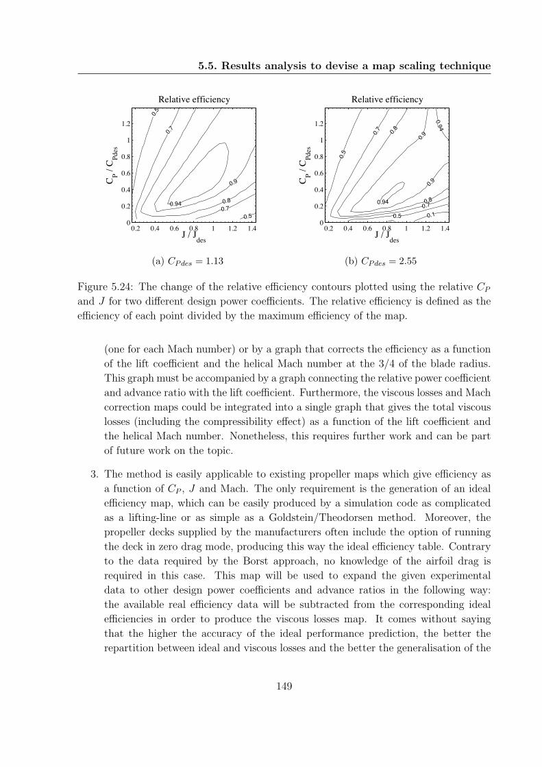
5.5. Results analysis to devise a map scaling technique

0.2 0.4 0.6 0.8 1 1.2 1.40

0.2

0.4

0.6

0.8

1

1.2

Relative efficiency

J / Jdes

C P / C Pd

es

0.5

0.5

0.7

0.70.8

0.9

0.94

(a) CPdes = 1.13

0.2 0.4 0.6 0.8 1 1.2 1.40

0.2

0.4

0.6

0.8

1

1.2

Relative efficiency

J / Jdes

C P / C Pd

es

0.10.5

0.5

0.7

0.7

0.8

0.8

0.9

0.9

0.94

0.94

(b) CPdes = 2.55

Figure 5.24: The change of the relative efficiency contours plotted using the relative CPand J for two different design power coefficients. The relative efficiency is defined as the

efficiency of each point divided by the maximum efficiency of the map.

(one for each Mach number) or by a graph that corrects the efficiency as a function

of the lift coefficient and the helical Mach number at the 3/4 of the blade radius.

This graph must be accompanied by a graph connecting the relative power coefficient

and advance ratio with the lift coefficient. Furthermore, the viscous losses and Mach

correction maps could be integrated into a single graph that gives the total viscous

losses (including the compressibility effect) as a function of the lift coefficient and

the helical Mach number. Nonetheless, this requires further work and can be part

of future work on the topic.

3. The method is easily applicable to existing propeller maps which give efficiency as

a function of CP , J and Mach. The only requirement is the generation of an ideal

efficiency map, which can be easily produced by a simulation code as complicated

as a lifting-line or as simple as a Goldstein/Theodorsen method. Moreover, the

propeller decks supplied by the manufacturers often include the option of running

the deck in zero drag mode, producing this way the ideal efficiency table. Contrary

to the data required by the Borst approach, no knowledge of the airfoil drag is

required in this case. This map will be used to expand the given experimental

data to other design power coefficients and advance ratios in the following way:

the available real efficiency data will be subtracted from the corresponding ideal

efficiencies in order to produce the viscous losses map. It comes without saying

that the higher the accuracy of the ideal performance prediction, the better the

repartition between ideal and viscous losses and the better the generalisation of the

149

References

[1] Advisory Council for Aeronautics Research in Europe (ACARE). European aero-
nautics: A vision for 2020, January 2001.
[2] N. T. Birch. 2020 vision: the prospects for large civil aircraft propulsion. Aeronau-
tical Journal, 104(1038):347–352, 2000.
[3] J. A. Borradaile. Towards the optimum ducted uhbr engine. In Proceedings of
24th AIAA/ASME/SAE/ASEE Joint Propulsion Conference and Exhibit, number
AIAA-88-2954, Boston, Massachusetts, July 1988.
[4] N. J. Peacock and J. H. R. Sadler. Advanced propulsion systems for large subsonic
transports. Journal of Propulsion and Power, 8(3), May-June 1992.
[5] D. L. Daggett, S. T. Brown, and R. T. Kawai. Ultra-efficient engine diameter study.
Technical Report CR-2003-212309, NASA, 2003.
[6] M. T. Tong. An assessment of the impact of emerging high-temperature materials
on engine cycle performance. In Proceedings of the ASME Turbo Expo, number
GT2010-22361, Glasgow, Scotland, June 2010. ASME.
[7] A. J. B. Jackson. Some future trends in aero engine design for sub-sonic transport.
Journal of Engineering for Power, 98:281–289, April 1976.
[8] R. A. Zimbrick and J. L. Colehour. An investigation of very high bypass ratio
engines for subsonic transports. In Proceedings of 24th AIAA/ASME/SAE/ASEE
Joint Propulsion Conference and Exhibit, Boston, Massachusetts, July 1988.
[9] V. E. Kyritsis. Thermodynamic preliminary design of civil turbofans and variable
geometry implementation. PhD thesis, Cranfield University, School of Engineering,
Dept of Power and Propulsion, 2006.
[10] C. Riegler and C. Bichlmaier. The geared turbofan technology - opportunities,
challenges and readiness status. Technical report, MTU Aero Engines GmbH, 2008.
165
[11] P. Laskaridis. Performance Investigations and Systems Integration for the More
Electric Aircraft. PhD thesis, Power and Propulsion Dept., Cranfield University,
2004.
[12] M. A. Dornheim. Electric cabin: The 787 generates at least four times more elec-
tricity than normal. traditionally bleed-powered systems now use volts, 28 March
2005.
[13] B. Sweetman. Unlaunched a350 jet takes shape very publicly. Aviation Week Show
News, Paris Air Show 2005, 13 June 2005.
[14] P. Laskaridis. Effects of engine parameters on secondary power extraction and
evaluation of engine performance penalties. In AIAA 19th International Symposium
on Air Breathing Engines (ISABE), number ISABE-2009-1275, Montreal, Canada,
2009.
[15] R. Slingerland and S. Zandstra. Bleed air versus electric power off-takes from a
turbofan gas turbine over the flight cycle. In AIAA 7th Aviation Technology, In-
tegration and Operations Conference (ATIO), number AIAA 2007-7848, Belfast,
Northern Ireland, 2007.
[16] R. Gandolfi, L. F. Pellegrini, and S. de Oliveira. More electric aircraft analysis
using exergy as a design comparison tool. In AIAA 48th Aerospace Sciences Meeting
Including the New Horizons Forum and Aerospace Exposition, number AIAA 2010-
809, Orlando, Florida, 2010.
[17] A. J. B. Jackson. Optimisation of aero and industrial gas turbine design for the
environment. PhD thesis, School of Engineering, Cranfield University, 2009.
[18] R. D. Hager and D. Vrabel. Advanced turboprop project. Technical Report SP-495,
NASA, 1988.
[19] M. T. Tong, D. R. Thurman, and M. D. Guynn. Conceptual design study of an
advanced open-rotor propulsion system. In Proceedings of the 20th International
Symposium on Air Breathing Engines, number ISABE-2011-1311, Goteberg, Swe-
den, September 2011. AIAA.
[20] E. S. Hendricks. Development of an open rotor cycle model in npss using a multi-
design point approach. In Proceedings of ASME Turbo Expo, number GT2011-46694,
Vancouver, Canada, June 2011. ASME.
[21] M. D. Guynn, J. J. Berton, E. S. Hendricks, M. T. Tong, J. W. Haller, and D. R.
Thurman. Initial assessment of open rotor propulsion applied to an advanced
166
single-aisle aircraft. In 11th AIAA Aviation Technology, Integration, and Oper-
ations (ATIO) Conference, Virginia Beach, VA; United States, September 2011.
NASA.
[22] A. Seitz, D. Schmitt, and S. Donnerhack. Emission comparison of turbofan and open
rotor engines under special consideration of aircraft and mission design aspects. The
Aeronautical Journal, 115(1168):351–360, June 2011.
[23] A. Seitz. Advanced Methods for Propulsion System Integration in Aircraft Concep-
tual Design. PhD thesis, Technische Universitat Munchen, 2011.
[24] C. A. Perullo, J. C. M. Tai, and D. N. Mavris. Effects of advanced engine technology
on open rotor cycle selection and performance. In Proceedings of ASME Turbo Expo,
number GT2012-69331, Copenhagen, Denmark, June 2012. ASME.
[25] R. C. Wilcock, J. B. Young, and J. H. Horlock. Gas properties as a limit to gas
turbine performance. In Proceedings of the ASME Turbo Expo, number GT-2002-
30517, 2002.
[26] A. Guha. Effects of internal combustion and non-perfect gas properties on the opti-
mum performance of gas turbines. Proceedings of the Inst. of Mechanical Engineers,
Part C: J. Mechanical Engineering Science, 217:1085–1099, 2003.
[27] J. Kurzke. Achieving maximum thermal efficiency with the simple gas turbine cycle.
In Proceedings of the 9th CEAS European Propulsion Forum: ”Virtual Engine - A
challenge for integrated computer modelling”, Roma, Italy, October 2003.
[28] P. P. Walsh and P. Fletcher. Gas turbine performance. Blackwell Science, 2nd
edition, 2004.
[29] A. Guha. Optimization of aero gas turbine engines. Aeronautical Journal,
105(1049):345–358, 2001.
[30] H. W. Bennett. Aero engine development for the future. Proceedings of the Inst. of
Mechanical Engineers, Part A: Power and Process Engineering, 197:149–157, July
1983.
[31] E. Schwartz and C. Hall. Assessment of future aircraft technologies on engine noise
and fuel consumption. In AIAA 18th International Symposium on Air Breathing
Engines (ISABE), number ISABE-2007-1142, Beijing, China, 2007.
[32] L. R. Jenkinson, P. Simpkin, and D. Rhodes. Civil jet aircraft design. Arnold, 1999.
167
[33] G. C. Oates. Aerothermodynamics of Gas Turbine and Rocket Propulsion. AIAA
Education Series, Washington, DC, revised and enlarged edition edition, 1988.
[34] A. Guha. Optimum fan pressure ratio for bypass engines with seperate or mixed
exhaust streams. Journal of Propulsion and Power, 17(5), 2001.
[35] B. G. Bruni. Performance investigations of turbofan aero engines. Master’s thesis,
School of Engineering, Cranfield University, 2010.
[36] J. Kurzke. Fundamental differences between conventional and geared turbofans. In
Proceedings of ASME Turbo Expo, number GT2009-59745. ASME, 2009.
[37] R. E. Owens, K. L. Hasel, and D. E. Mapes. Ultra high bypass turbofan technologies
for the twenty-first century. In Proceedings of 26th AIAA/ASME/SAE/ASEE Joint
Propulsion Conference, number AIAA-90-2397, Orlando, Florida, July 1990.
[38] P. H. Young. The future shape of medium and long-range civil engines. Aeronautical
Journal, February 1979.
[39] G. L. Wilde. Future large civil turbofans and powerplants. Aeronautical Journal,
82:281–299, July 1978.
[40] D. J. Karanja and R. A. Harvey. Optimization studies for the pw305 turbofan. In
Proceedings of 26th AIAA/ASME/SAE/ASEE Joint Propulsion Conference, num-
ber AIAA 90-2520, Orlando, Florida, 1990.
[41] J-M. Jacquet and D. L. Seiwert. Methodology for commercial engine/aircraft opti-
mization. In Proceedings of 29th AIAA/SAE/ASME/ASEE Joint Propulsion Con-
ference and Exhibit, number AIAA 93-1807, Monterey, CA, 1993.
[42] Cranfield University. The turbomatch scheme, October 1999.
[43] W. H. Press, S. A. Teukolsky, W. T. Vetterling, and B. P. Flannery. Numerical
Recipes in Fortran 90. Cambridge University Press, 1996.
[44] H. I. H. Saravanamuttoo, G. F. C. Rogers, and H. Cohen. Gas turbine theory.
Prentice Hall, 5th edition, 2001.
[45] P. Lolis. Preliminary gas turbine weight estimation methods. PhD thesis, Cranfield
University, 2013.
[46] L. Davis, editor. Handbook of genetic algorithms. Van Nostrand Reinhold, New
York, US, 1991.
168
[47] M. Gen and R. Cheng. Genetic algorithms and engineering optimization. John
Wiley and Sons Inc., Chichester, UK, 2000.
[48] J. M. Rogero. A genetic algorithms-based optimisation tool for the preliminary
design of gas turbine combustors. PhD thesis, School of Engineering, Cranfield
University, 2002.
[49] C. Celis. Evaluation and optimisation of environmentally friendly aircraft propulsion
systems. PhD thesis, School of Engineering, Cranfield University, 2010.
[50] T. Gronstedt. Advanced solvers for general high performance transient gas tur-
bine simulation tools. In 14th International Symposium on Air Breathing Engines,
Florence, Italy, September 1999.
[51] M. W. Whellens, R. Singh, and P. Pilidis. Genetic algorithm based optimisation
of intercooled recuperated turbofan design. In Proceedings of 41st AIAA Aerospace
Sciences Meeting and Exhibit, number AIAA 2003-1210, Reno, Nevada, January
2003. AIAA.
[52] A. Gulati. An optimisation tool for gas turbine engine diagnostics. PhD thesis,
School of Engineering, Cranfield University, 2001.
[53] S. Sampath. Fault diagnostics for advanced cycle marine gas turbine using genetic
algorithms. PhD thesis, School of Engineering, Cranfield University, 2003.
[54] M. W. Whellens. Multidisciplinary optimisation of aero-engines using genetic algo-
rithms and preliminary design tools. PhD thesis, School of Engineering, Cranfield
University, 2003.
[55] P. Jeschke, J. Kurzke, R. Schaber, and C. Riegler. Preliminary gas turbine design
using the multidisciplinary design system mopeds. In Proceedings of the ASME
Turbo Expo, number GT-2002-30496, Amsterdam, The Netherlands, June 2002.
[56] V. E. Kyritsis and P. Pilidis. Performance evaluation for the application of variable
turbine-cooling-bleeds in civil turbofans. In Proceedings of the ASME Turbo Expo,
number GT2007-27224, Montreal, Canada, May 2007.
[57] V. E. Kyritsis and P. Pilidis. Principles of thermodynamic preliminary design of civil
turbofan engines. In Proceedings of the ASME Turbo Expo, number GT2009-58815,
Orlando, Florida, June 2009. ASME.
[58] J. Kurzke. Preliminary design. Lecture Series 2002-2003, Aero-engine design: a
state of the art. von Karman Institute for Fluid Dynamics, April 2003.
169
[59] J. Kurzke. Gas turbine cycle design methodology: A comparison of parameter
variation with numerical optimization. Journal of Engineering for Gas Turbines
and Power, 121, January 1999.
[60] S. Kawada. Calculation of induced velocity by helical vortices and its application
to propeller theory. Technical Report 172, Aeronautical Research Institute, Tokyo
Imperial University, 1939.
[61] J. S. Schutte. Simultaneous multi-design point approach to gas turbine on-design
cycle analysis for aircraft engines. PhD thesis, Georgia Institute of Technology,
[62] B. Gunston. Jane’s: Aero-engines. Jane’s Information Group, 2010.
[63] D. Riordan. Environmentally friendly engine nacelle technology devel-
opment. http://flygreen.info/wp-content/uploads/2012/10/bombardier_
driordan_ppt_w2.pdf, 2012 (Accessed on 28/04/2013).
[64] S. Lott. One giant leap. http://www.aero-mag.com/features/19/20121/1206/,
2012 (Accessed on 28/04/2013).
[65] A. Schonland. The foundation behind the leap-x. http://airinsight.com/2011/
01/31/the-foundation-behind-the-leap-x/, 2011 (Accessed on 28/04/2013).
[66] Low density materials. http://www.rolls-royce.com/about/technology/
material_tech/low_density_materials.jsp, Accessed on 28/04/2013.
[67] Leap-x, a trailblazer for tomorrow’s aero-engines. http://www.safran-group.com/
IMG/pdf/EN_mag5_p8-9-2.pdf, 2009 (Accessed on 28/04/2013).
[68] E. S. Arvai. Comparing the new technology narrow-body engines: Gtf vs leap
maintenance costs. http://airinsight.com/2011/11/09/, 2011 (Accessed on
13/03/2013).
[69] A. G. Hoffman, I. G. Hansen, R. F. Beach, R. M. Plencher, R. P. Dengler, K. S.
Jefferies, and R. J. Frye. Advanced secondary power system for transport aircraft.
Technical Report 2463, NASA, May 1985.
[70] G.E. Tagge, L. A. Irish, and A. R. Bailey. Systems study for an integrated digi-
tal/electric aircraft (idea). Technical Report NASA CR 3840, Boeing Commercial
Airplane Company, 1985.
[71] M. J. Cronin, A. P. Hays, F. B. Green, N. A. Radovcich, C. W. Helsley, and W. L.
Rutchik. Integrated digital/electric aircraft concepts study. Technical Report NASA
CR 3841, Lockheed California, 1985.
170
[72] R. I. Jones. Considerations of the all electric (accessory) engine concept. Pro-
ceedings of the Institution of Mechanical Engineers, Part G: Journal of Aerospace
Engineering, 209, 1995.
[73] R. I. Jones. The more electric aircraft—assessing the benefits. Proceedings of the
Institution of Mechanical Engineers, Part G: Journal of Aerospace Engineering,
216(5):259–269, 2002.
[74] G. Codner. The implication of advanced engines for the airframe systems of trans-
port aircraft. Master’s thesis, Aircraft Design Dept., Cranfield University, 1988.
[75] G. B. Toyne and G. S. Hodges. ’all-electric’ accessory drive systems: Implications
on engine design and performance. In In Auxiliary Power Systems Meeting, volume
AGARD CP-352, Copenhagen, 1983.
[76] H. M. Helm. Study of a zero bleed engine and a new secondary power system for
large aircraft. Technical Report RR-PNR-92634, Rolls-Royce plc., 1999.
[77] T. R. Ensign. Sensitivity studies of electric systems on business jet range. In
AIAA 46th Aerospace Sciences Meeting and Exhibit, number AIAA 2008-147, Reno,
Nevada, 2008.
[78] R. D. Archer and M. Saarlas. An Introduction to Aerospace Propulsion, chapter 3,
pages 68–127. Prentice Hall, 1996.
[79] H. S. Wainauski, C. Rohrbach, and T.A. Wynosky. Prop-fan performance termi-
nology. In Proceedings of Aerospace Technology Conference and Exposition, number
871838, Long Beach, California, October 1987. Society of Automotive Engineers.
[80] D. C. Mikkelson, G. A. Mitchell, and L. Bober. Summary of recent nasa propeller
research. Technical Report TM-83733, NASA, 1984.
[81] R. Worobel and M. G. Mayo. Advanced general aviation propeller study. Technical
Report CR-114289, NASA, April 1971.
[82] D. C. Mikkelson, B. J. Blaha, G. A. Mitchell, and J. E. Wikete. Design and perfor-
mance of energy efficient propellers for mach 0.8 cruise. Technical Report 770458,
Society of Automotive Engineers, 1977.
[83] D. B. Hanson, C. J. McColgan, R. M. Ladden, and R. J. Klatte. Unified aeroacous-
tics analysis for high speed turboprop aerodynamics and noise. Technical Report
CR-185193, NASA, 1991.
171
[84] Q. R. Wald. The aerodynamics of propellers. Progress in Aerospace Sciences, 42:85–
128, 2006.
[85] W. J. M. Rankine. On the mechanical principles of the action of propellers. Trans
Inst Naval Architects (British), 6(13), 1865.
[86] R. E. Froude. Trans Inst Naval Architects, 30:390, 1889.
[87] O. Gur and A. Rosen. Comparison between blade-element models of propellers.
The Aeronautical Journal, 112(1138):689–704, December 2008.
[88] A. Rosen and O. Gur. Novel approach to axisymmetric actuator disk modeling.
AIAA Journal, 46(11):2914–2925, November 2008.
[89] H. Glauert. Aerodynamic Theory: A General Review of Progress, volume IV, chapter
Airplane Propellers, pages 169–310, 341–344. Julius Springer, 1935.
[90] S. Drzewiecki. Theorie generale de l’helice. Gauthier-Villars et cie., Paris, France,
1920.
[91] G. J. D. Zondervan. A review of propeller modelling techniques based on euler
methods. Technical Report LR-797, Delft University of Technology, November 1995.
[92] A. Betz and L. Prandtl. Schraubenpropeller mit geringstem energieverlust. Tech-
nical report, Goettinger Nachrichten, 1919.
[93] O. Gur and A. Rosen. Optimization of propeller based propulsion system. Journal
of Aircraft, 46(1):95–106, 2009.
[94] M. A. Takallu and D. M. Dunham. A hybrid method of prediction for propeller
performance. In Proceedings of 28th AIAA Aerospace Sciences Meeting, number
AIAA-90-0440, Reno, Nevada, January 1990. AIAA.
[95] W. Z. Stepniewski and C. N. Keys. Rotary-Wing Aerodynamics, chapter 4 - Vortex
Theory, pages 141–159. Dover Publications, 1984.
[96] J. D. Anderson. Fundamentals of Aerodynamics, pages 668–674. McGraw-Hill
International Edition, 4th edition, 2007.
[97] S. Goldstein. On the vortex theory of screw propellers. In Proceedings of the
Royal Society, volume 123 of A, Containing Papers of a Mathematical and Physical
Character, pages 440–465, 1929.
[98] Theodore Theodorsen. Theory of Propellers. McGraw-Hill Publications in Aero-
nautical Science, April 1954.
172
[99] H. V. Borst. Summary of propeller design procedures and data volume i: Aerody-
namic design and installation. Technical Report 73-34A, USAAMRDL, 1973.
[100] C. Rohrbach. A report on the aerodynamic design and wind tunnel test of a prop-fan
model. In Proceedings of 12th AIAA/SAE Propulsion Conference, number AIAA-
76-667, Palo Alto, California, July 1976. AIAA.
[101] F. B. Metzger and C. Rohrbach. Aeroacoustic design of the prop-fan. In Proceed-
ings of the 5th AIAA Aeroacoustics Conference, number AIAA-79-0610, Seattle,
Washington, March 1979. AIAA.
[102] Y. Sandak and A. Rosen. Aeroelastically adaptive propeller using blades’ root
flexibility. The Aeronautical Journal, pages 411–418, August 2004.
[103] R. J. Jeracki and G. A. Mitchell. Low and high speed propellers for general aviation
- performance potential and recent wind tunnel test results. Technical Report TM-
81745, NASA, 1981.
[104] D. M. Black, R. W. Menthe, and H. S. Wainauski. Aerodynamic design and perfor-
mance testing of an advanced 30o swept, eight bladed propeller at mach numbers
from 0.2 to 0.85. Technical Report CR-3047, NASA, 1978.
[105] C. Rohrbach, F. B. Metzger, D. M. Black, and R. M. Ladden. Evaluation of wind
tunnel performance testings of an advanced 45 swept eight-bladed propeller at mach
numbers from 0.45 to 0.85. Technical Report CR-3505, NASA, 1982.
[106] C. N. Adkins and R. H. Liebeck. Design of optimum propellers. Journal of Propul-
sion and Power, 10(5):676–682, September-October 1994.
[107] M. Olausson, R. Avellan, N. Sorman, F. Rudebeck, and L. Eriksson. Aeroacoustics
and performance modeling of a counter-rotating propfan. In Proceedings of ASME
Turbo Expo, number GT2010-22543, Glasgow, Scotland, June 2010. ASME.
[108] B. G. McKay. Ideal optimization of counterrotating propellers. In Proceedings of
24th ASME, SAE, ASEE Joint Propulsion Conference, number AIAA-1988-2801,
Boston, MA, July 1988.
[109] R. E. Davidson. Optimization and performance calculation of dual-rotation pro-
pellers. Technical Report TM-1948, NASA, 1981.
[110] W. F. Phillips and D. O. Snyder. Modern adaptation of prandtl’s classic lifting-line
theory. Journal of Aircraft, 37(4):662–670, July-August 2000.
173
[111] L. Bober and L. Chang. Factors influencing the predicted performance of advanced
propeller designs. Technical Report TM-82676, NASA, 1981.
[112] G. L. Stefko, L. J. Bober, and H. E. Neumann. New test techniques and analytical
procedures for understanding the behavior of advnaced propellers. Technical Report
TM-83360, NASA, 1983.
[113] L. J. Bober. Advanced propeller aerodynamic analysis. Technical report, NASA,
1980.
[114] L. J. Bober and G. A. Mitchell. Summary of advanced methods for predicting
high speed propeller performance. In Proceedings of 18th AIAA Aerospace Sciences
Meeting, number AIAA-80-0225, Pasadena, California, January 1980. AIAA.
[115] J. M. Bousquet. Etude de l’aerodynamique des helices pour avions rapides. In
Proceedings of Advanced Technology for Aero Gas Turbine Components AGARD
Conference, number CP-421. AGARD, 1987.
[116] W. A. Campbell, H. S. Wainauski, and P. R. Bushnell. A report on high speed
wind tunnel testing of the large scale advanced prop-fan. In Proceedings of
AIAA-88-2802, Boston, Massachusetts, July 1988. AIAA.
[117] T. A. Egolf, O. L. Anderson, D. E. Edwards, and A. J. Landgrebe. An analysis for
high speed propeller-nacelle aerodynamic performance prediction, volume i: Theory
and application. Technical Report CR-169450, NASA, 1988.
[118] J. P. Sullivan. The effect of blade sweep on propeller performance. In Proceedings of
the 10th AIAA Fluid and Plasma Dynamics Conference, number AIAA-1977-716,
Albuquerque, New Mexico, June 1977. AIAA.
[119] J. M. Bousquet. Theoretical and experimental analysis of highspeed propeller aero-
dynamics. In Proceedings of 22nd AIAA/ASME/SAE/ASEE Joint Propulsion Con-
ference and Exhibit, Huntsville, Alabama, June 1986.
[120] J. M. Bousquet. Methodes aerodynamiques utilisees en france pour l’etude des
helices pour avions rapides. In Proceedings of Aerodynamics and Acoustics of Pro-
pellers AGARD Conference, number CP-366. AGARD, 1984.
[121] J. M. Bousquet and P. Gardarein. Recent improvements in propeller aerodynamic
computations. In Proceedings of 18th AIAA Applied Aerodynamics Conference,
number AIAA-2000-4124. AIAA, 2000.
174
[122] L. Prandtl. Application of modern hydrodynamics to aeronautics. Technical Report
TR-116, NACA, 1923.
[123] C. Young. The prediciton of helicopter rotor hover performance using a prescribed
wake analysis. Technical Report CP 1341, Aeronautical Research Council, 1976.
[124] R. D. Clark and C. A. Leiper. The free wake analysis. a method for the prediction of
helicopter rotor hovering performance. Journal of the American Helicopter Society,
15(1):3–11, 1970.
[125] C. S. Chen, H. R. Velkoff, and C. Tung. Free-wake analysis of a rotor in hover. In
Proceedings of 19th AIAA Fluid Dynamics, Plasma Dynamics and Lasers Confer-
ence, number AIAA-87-1245, Honolulu, Hawaii, June 1987. AIAA.
[126] K. Karamcheti. Principles of Ideal-Fluid Aerodynamics. Krieger, 1980.
[127] J. G. Leishman. Principles of Helicopter Aerodynamics. Cambridge University
Press, 2nd edition, 2006.
[128] S. Bechet, C. A. Negulescu, V. Chapin, and F. Simon. Integration of cfd tools in
aerodynamic design of contra-rotating propeller blades. In CEAS 2011 The Inter-
national Conference of the European Aerospace Societies, 2011.
[129] C. Burger. Propeller performance analysis and multidisciplinary optimization using
a genetic algorithm. PhD thesis, Auburn University, Auburn, Alabama, 2007.
[130] G. Iosifidis. Single-rotation advanced performance modelling. Master’s thesis,
School of Engineering, Cranfield University, 2011.
[131] A. Sanchez-Ortega. Performance modelling of advanced propellers. Master’s thesis,
Cranfield University, School of Engineering, 2011.
[132] L. L. Erickson. Panel methods - an introduction. Technical Paper 2995, NASA,
1990.
[133] L. Morino, editor. Computational Methods in Potential Aerodynamics. Springer-
Verlag, 1985.
[134] M. Tremmel, D. B. Taulbee, and J. R. Sonnenmeier. Numerical determination of
circulation for a swept propeller. Journal of Aircraft, 38(6):1085–1092, November-
December 2001.
[135] C. J. Szymendera. Computational free wake analysis of a helicopter rotor. Master’s
thesis, The Pensylvania State University, Dept of Aerospace Engineering, May 2002.
175
[136] S. Ananthan, J. G. Leishman, and M. Ramasamy. The role of filament stretching in
the free-vortex modeling of rotor wakes. In Proceedings of the 58th Annual Forum
and Technology Display of the American Helicopter Society International, Montreal,
Canada, June 2002. American Helicopter Society.
[137] A. F. Donovan and H. R. Lawrence, editors. Aerodynamic Components of Aircraft
at High Speeds, volume Volume VII High Speed Aerodynamics and Jet Propulsion.
Princeton University Press, 1957.
[138] E. Sand, D. A. Elliott, and H. V. Borst. Summary of propeller design procedures
and data volume iii: hub, actuator and control designs. Technical Report 73-34C,
USAAMRDL, Fort Eustis, VA, November 1973.
[139] C. M. Maksymiuk and S. A. Watson. A computer program for estimating the
aerodynamic characteristics of naca 16-series airfoils. Technical Report TM-85696,
NASA, 1983.
[140] O. Gur and A. Rosen. Propeller performance at low advance ratio. Journal of
Aircraft, 42(2):435–441, March-April 2005.
[141] T. Von Karman. Supersonic aerodynamics - principles and applications. Journal of
the Aeronautical Sciences, 14(7), 1947.
[142] R. E. Davidson. Linearized potential theory of propeller induction in a compressible
flow. Technical Note 2983, NACA, 1953.
[143] V. L. Wells. Propellers in compressible flow. In Proceedings of 14th Congress of
the International Council of the Aeronautical Sciences, pages 697–707, Toulouse,
France, September 1984. ICAS, American Institute of Aeronautics and Astronautics.
[144] J. C. Evvard. Distribution of wave drag and lift in the vicinity of wing tips at
supersonic speeds. Technical Report TN-1382, NACA, July 1947.
[145] D. B. Hanson. Compressible helicoidal surface theory for propeller aerodynamics
and noise. AIAA Journal, 21(6):881–889, June 1983.
[146] D. B. Hanson. Compressible lifting surface theory for propeller performance calcu-
lation. Journal of Aircraft, 22(1), January 1985.
[147] R. L. Bisplinghoff, H. Ashley, and R. L. Halfman. Aeroelasticity. Dover Publications,
1996.
[148] G. L. Stefko and R. J. Jeracki. Wind-tunnel results of advanced high- speed pro-
pellers at takeoff, climb, and landing mach numbers. Technical Report TM-87030,
NASA, November 1985.
176
[149] L. J. Bober, D. S. Chaussee, and P. Kutler. Prediction of high speed propeller flow
fields using a three-dimensional euler analysis. Technical Report TM-83065, NASA,
[150] R. J. Jeracki, D. C. Mikkelson, and B. J. Blaha. Wind tunnel performance of four
energy efficient propellers designed for mach 0.8 cruise. Technical Report TM-79124,
NASA, 1979.
[151] R. M. Plencher, P. Senty, and T.J. Wickenheiser. Propeller performance and weight
predictions appended to the navy/nasa engine program. Technical Report TM-
83458, NASA, 1983.
[152] S.B.A.C. Standard method of propeller performance estimation. Technical report,
Society of British Aircraft Constructors Ltd., 1943.
[153] L. K. Chang and J. P. Sullivan. Optimization of propeller blade twist by an ana-
lytical method. AIAA Journal, 22(2):252–255, February 1984.
[154] J. Cho and S. C. Lee. Propeller blade shape optimization for efficiency improvement.
Computers & Fluids, 27(3):407–419, 1998.
[155] P. Giannakakis, P. Laskaridis, and P. Pilidis. Effects of offtakes for aircraft
secondary-power systems on jet engine efficiency. Journal of Propulsion and Power,
27(5), 2011.
177
Related Documents