1 Crack Propagation Analysis of Mode--I Fracture in Pultruded Composites using Micromechanical Constitutive Models Rami Haj--Ali andRani El--Hajjar School of Civil and Environmental Engineering Georgia Institute of Technology, Atlanta, GA 30332--0355 [email protected], [email protected] ABSTRACT An experimental and analytical study is carried out to characterize the fracture behavior of fiber reinforced plastic (FRP) pultruded composites. The composite material system used in this study consists of roving and continuous filament mat (CFM) layers with E--glass fiber and polyester matrix. Eccentrically loaded single--edge--notch--tension ESE(T) fracture toughness specimen were cut from a thick pultruded plate, with the roving orientation trans- verse to the loading direction. Three--dimensional (3D) micromechanical constitutive mod- els for the CFM and roving layers are developed. The micromodels can generate the effec- tive nonlinear behavior while recognizing the in--situ response at the fiber and matrix levels. The ability of the proposed micromodels to predict the effective elastic properties as well as the nonlinear response under multi--axial stress states is verified and compared to the stress-- strain response from a series of off--axis tests. The micromodels are implemented in a finite element (FE) code with a cohesive layer to model the nonlinear fracture behavior of a pul- truded composite material with different crack configurations. The properties for the cohe- sive layer were calibrated from one ESE(T) specimen with a crack to width ratio, a/W of 0.5. Good prediction is demonstrated for a range of notch sizes and geometries. The use of cohe- sive elements with nonlinear micromodels is effective in modeling the transverse mode--I crack growth behavior in pultruded composites.

Welcome message from author
This document is posted to help you gain knowledge. Please leave a comment to let me know what you think about it! Share it to your friends and learn new things together.
Transcript

1
Crack Propagation Analysis of Mode--I Fracture in PultrudedComposites using Micromechanical Constitutive Models
Rami Haj--Ali and Rani El--Hajjar
School of Civil and Environmental Engineering
Georgia Institute of Technology, Atlanta, GA 30332--0355
[email protected], [email protected]
ABSTRACT
An experimental and analytical study is carried out to characterize the fracture behavior
of fiber reinforced plastic (FRP) pultruded composites. The compositematerial systemused
in this study consists of roving and continuous filamentmat (CFM) layers with E--glass fiber
and polyester matrix. Eccentrically loaded single--edge--notch--tension ESE(T) fracture
toughness specimen were cut from a thick pultruded plate, with the roving orientation trans-
verse to the loading direction. Three--dimensional (3D)micromechanical constitutivemod-
els for the CFM and roving layers are developed. The micromodels can generate the effec-
tive nonlinear behavior while recognizing the in--situ response at the fiber and matrix levels.
The ability of the proposed micromodels to predict the effective elastic properties as well as
the nonlinear response under multi--axial stress states is verified and compared to the stress--
strain response from a series of off--axis tests. The micromodels are implemented in a finite
element (FE) code with a cohesive layer to model the nonlinear fracture behavior of a pul-
truded composite material with different crack configurations. The properties for the cohe-
sive layer were calibrated from one ESE(T) specimenwith a crack towidth ratio, a/W of 0.5.
Good prediction is demonstrated for a range of notch sizes and geometries. The use of cohe-
sive elements with nonlinear micromodels is effective in modeling the transverse mode--I
crack growth behavior in pultruded composites.

2
INTRODUCTION
Pultrusion is a manufacturing process whereby different types of fiber reinforcements
are guided from a creel, impregnated with resin, drawn through a preform block through a
heated die for curing. Pultruded composite structural members can have a general constant
cross--sectional profile similar to standard profiles found in metallic frames, e.g. I--shapes,
tubes, and angles. Pultruded composites are thick heterogeneousmaterials that can combine
various forms of reinforcement systems repeated through the thickness of the member, such
as roving, continuous filamentmats (CFM),woven fabrics, and braided preforms. Currently
CFM and roving reinforcements are widely used. The CFM layer consists of relatively long
and swirled filaments that are randomly oriented in the plane of the layer. TheCFM is usual-
ly used for multi--directional secondary reinforcement and to provide material continuity in
transition regions of the cross--section, e.g. near the web--flange junction in an I--shape pul-
truded member.
Production of pultruded composites may result in a number of manufacturing defects
such asmatrixmicrocracks and voids. Voids andmicrocracks can grow and coalesce to form
a crack on the macroscopic level and may cause catastrophic failure. The anisotropic nature
of pultruded composites also results in anisotropic fracture properties. A crack propagating
transverse to the roving direction is restrained by the bridging effect of the unidirectional
roving fibers. The unidirectional roving layer is the major reinforcement system used in the
cross--section. This makes the transverse direction have the lowest fracture toughness.
Stress based failure criteria have been proposed to determine the strength of notched
composites. Some of these criteria are evaluated pointwise while others are determined us-
ing average variables or a characteristic length. Whitney and Nussimer (1974) proposed a
failure criterion based on the average stress distribution calculated from the edge of the hole
to a given characteristic distance. The distance from the edge is considered as a material
property and does not depend on the size of the notch. A second related criterion is based

3
on assuming failure to occur when the stress at a distance away from the notch reaches the
strength of the unnotched material. The proposed criteria were applied to graphite/epoxy
and glass/epoxy laminated composites with straight cracks and used to explain the reduction
in strength of composites with larger hole sizes. Sih et al. (1975) proposed a strain energy
density failure criterion to predict fracture in unidirectional composites subject to off--axis
loading.
Despite limitations such as the violation of self--similar crack growth in various lami-
nates, Linear Fracture Mechanics (LFM) has been successfully applied to study failure in
different composite systems (Parhizgar et al., 1982 and Konish et al., 1972). Waddoups et
al. (1971) used a stress intensity factor (SIF) calculated based on amodified crack size. The
larger effective crack length is determined based on equating the intense energy region ahead
of the crack to amaterial dependent characteristic length. Holdsworth et al. (1974) usedLFM
to predict the fracture of notched plates and box--section beams made from Chopped Strand
Mat (CSM)with glass fibers and polyester resin. An effective crack size approachwas used,
similar toWaddoups et al. (1971). The effective crack lengthwas determined based onmodi-
fying the initial diameter of the notched holes. Mandell et al. (1974) used hybrid finite ele-
ment (FE) analysis to show that the SIF can be strongly dependent on the degree of material
anisotropy for various specimen geometries. The SIF change between isotropic and aniso-
tropic cases is relatively constant for varying crack lengths in a given geometry. Sih et al.
(1965) used a complex variable approach to derive the general equations of crack--tip stress
fields in anisotropic bodies. The material constants were found to have an effect on the
crack--tip stresses. Kanninen et al. (1977a, 1977b) reviewed the applicability of fractureme-
chanics in composite materials and advocated the merging of a micromechanical failure
analysis with a macromechanical analysis. The material was considered heterogeneous
where microstructural effects are predominant and as a homogenous anisotropic continuum
where it is not.

4
Pultruded materials and structures may exhibit nonlinear material behavior when sub-
jected to multi--axial loading. The primary causes of this behavior are the soft response of
the polymeric matrix and the presence of voids and microcracks. These nonlinear effects
are enhanced due to geometric and material discontinuities at the structural level. Cracks
in the pultruded structure can add to this nonlinear response. Thus, there exists a need for
nonlinear constitutive models capable of predicting the effective response under a general
multi--axial state of loading. This will allow studying the effect of nonlinearity on the frac-
ture process.
This study presents a combined modeling approach using micromechanical constitutive
and cohesive fracture models for the crack propagation analysis in thick--section pultruded
composites. The first part of this paper introduces new 3D--micromechanical constitutive
models for pultruded composites to generate the effective nonlinear multi--axial response
based on in situmatrix and fiber properties. The proposedmicromodels are derived and cali-
brated for an E--glass/Polyester fiber reinforced plastic (FRP) pultruded composite. Predic-
tion of the nonlinearmaterial response is then verified by testing a series of off--axis coupons
cut from a monolithic pultruded plate. The second part is an investigation of the through--
thickness mode--I fracture along the roving direction (transverse fracture) in the pultruded
material system. Test results in the form of load versus notch mouth opening displacement
(NMOD) from eccentrically loaded single--edge--notch tension ESE(T) and single--edge--
notch tension SEN(T) specimenwere used to calibrate and verify the proposed fracturemod-
eling approach.
PULTRUDED COMPOSITE MATERIAL SYSTEM
The pultruded composite material modeled in this study consists of a resin system rein-
forced with unidirectional roving and continuous filament mats. The roving layers are rein-
forcedwith unidirectional fiber bundles that can be distributed in designated locationswithin
the medium. Figure 1(a) shows a side view cross--section illustrating the layered nature of

5
this composite. Figure 1(b) shows a top view of a sectioned coupon exposing the CFM and
roving layers. The CFM and roving layers can have different thicknesses throughout the
cross--section. The material is idealized as a perfectly bonded layered system consisting of
roving and CFM layers. In addition to these constituents, there is an appreciable number of
voids spread inside the pultruded section. These voids tend to concentrate at the center of
the section. Matrix burn--out tests were conducted for E--glass/Vinylester pultruded com-
posites to determine the fiber volume fractions (FVFs) in the unidirectional roving andCFM
layers (Haj--Ali et al., 2002a). Similar burn--out tests were conducted for the E--glass/poly-
ester system. The calculated FVF values for the layers are: 0.407 for the roving and 0.305
for theCFM. These are averageFVFvalues over all the roving andCFMlayers, respectively.
The total average of E--glass FVF in the material (from both the roving and CFM volumes)
is 0.34.
NESTED MICROMECHANICAL CONSTITUTIVE FRAMEWORK
Nonlinear 3D micromechanical models are proposed to generate the effective response
for the roving and CFM layers. The two micromodels explicitly recognize the response of
the fiber and matrix constituents. The nonlinear micromechanical formulation, calibration,
and verification of these micromodels for E--glass/Vinylester composite materials were re-
ported by Haj--Ali et al. (2002a, 2002b). A similar 3D micromechanical framework is pro-
posed and integrated with FE fracture models for the fracture analysis of pultruded compos-
ites. The proposed modeling approach is schematically illustrated in Figure 2. It describes
a number of nested micromodels for each of the composite systems that exist within the
thickness of the cross--section. This approach is integrated with plane--strain or plane--stress
2D continuum finite element models by adding the appropriate constraints to the overall for-
mulation. The nonlinear response of the pultruded structure is sampled at material points
(Gaussian integration points) for each element in the FE model. The homogenized equiva-
lent continuum is generated for a periodic sequence of two alternating layers through the

6
thickness of each section. This level of the model is referred to as the sublaminate model.
It employs the 3D lamination theory to generate a nonlinear continuum response for theCFM
and the roving layers. The homogenization is performed at each material point in the thick-
ness directionwhich is the the third axis in the localmaterial orientation system attachedwith
each finite element, as shown in Figure 2. In the case where a plane stress state exists, the
CFM and roving 3Dmicromodels will be constrained to have zero out--of--plane overall av-
erage stress.
A general nonlinear sublaminatemodel was derived byHaj--Ali and Pecknold (1996) for
laminated composites. The current sublaminatemodel is used to generate an equivalent con-
tinuum response for roving and CFM layers. This is done using in--plane and out--of--plane
applied patterns of stress and strain. The 3D lamination theory is usedwith the same assump-
tions of Pagano (1974) and Sun and Li (1988). The stress and strain vectors for each layer
are partitioned into in--plane and out--of--plane components:
σi= σ11 σ22 τ12 , σo= σ33 τ13 τ23 (1)
εi= ε11 ε22 γ12 , εo= ε33 γ13 γ23 (2)
where the overbars indicate homogenized sublaminate quantities.
The assumption of a perfect bond between adjacent layers requires displacement conti-
nuity which leads to the continuous in--plane strains ( Á11, Á22, γ12 ) across their interface.
The traction continuity across the interface requires that the out--of--plane stresses
( σ33, τ13, τ23 ) to be continuous across the interface. As a result, the in--plane strains and
out--of--plane stresses are the same throughout the sublaminate for an applied hybrid in--
plane strain and out--of--plane stress. This is expressed by:

7
σo= σ(C)o = σ
(R)o (3)
εi= ε(C)
i= ε(R)
i (4)
where (C) and (R) denote CFM and roving layers, respectively.
The complementary stress and strain components may differ in the roving and CFM lay-
ers. The homogenized in--plane stresses and out--of--plane strains are taken as the weighted
averages, using the relative CFM and roving thickness, tC and tR, respectively, as:
σi=1
( tC+ tR ) tC σ(C)
i+ tR σ
(R)
i (5)
εo= 1( tC+ tR )
tC ε(C)o + tR ε(R)o (6)
Equations (3) to (6), along with the constitutive stress--strain relations for each layer,
characterize the sublaminate model. The roving and CFM sequence information is not pre-
served in this procedure. In the casewhere this sequence is important, the sublaminatemodel
is not used. Instead, the response of each layer is sampled several times through its cross
section. The section response is generated by numerical integration in a ply--by--ply ap-
proach.
MICROMECHANICAL MODEL FOR THE ROVING LAYERS
The unidirectional roving layer is idealized as a doubly periodic array of fibers with rec-
tangular cross--section embedded in the matrix. The long fibers are aligned in the x1 direc-
tion. The other cross--section directions are referred to as the transverse directions. A rectan-
gular unit cell geometry is proposed and shown in Figure 2. The traction and displacement
continuity between the subcells are approximated by using the average stress and strain com-
8
ponents of the four subcells. This approach makes the average stress and strain vectors as
the state variables.
The notation for the stress and strain vectors, defined for the 4--cell model are:
Á(α)i= [ Á11, Á22, Á33, γ12, γ13, γ23 ]
T
i = 1, .., 6
α = 1, .., 4
σ(α)i= [ σ11, σ22, σ33, τ12, τ13, τ23 ]
T
(7)
where (α) denotes a subcell number and (i) denotes a stress or strain component.
The relative volumes of the four subcells are:
v1 = h b ; v4 = (1− h) (1− b)v2 = (1− h) b ; v3 = h (1− b) ; (8)
Compatibility in the axial direction dictates that the average axial strains are the same
in all subcells. Therefore, the longitudinal (mode--1) micromechanical relations are:
Á(1)1= Á(2)
1= Á(3)
1= Á(4)
1= Á(R)
1
v1 σ(1)1+ v2 σ
(2)1+ v3 σ
(3)1+ v4 σ
(4)1= σ(R)1
(9)
Traction continuity along interfaces with normals in the x2 direction, yields the follow-
ing relations in terms of the stress components:
σ(1)2= σ(2)
2
σ(3)2= σ(4)
2
σ(1)4= σ(2)
4
σ(3)4= σ(4)
4
σ(1)6= σ(2)
6
σ(3)6= σ(4)
6
(a)
(b)
(c)
(10)

9
The corresponding strain compatibility relations are:
v1v1+ v2
Á(1)2+
v2v1+ v2
Á(2)2= Á(R)
2
v3v3+ v4
Á(3)2+
v4v3+ v4
Á(4)2= Á(R)
2
(a)
(11)
v1v1+ v2
Á(1)4+
v2v1+ v2
Á(2)4= Á(R)
4
v3v3+ v4
Á(3)4+
v4v3+ v4
Á(4)4= Á(R)
4
(b)
Traction continuity consideration for interfaces with normals in the x3 direction, yields
the following conditions for out--of--plane stress components:
σ(1)3= σ(3)
3
σ(2)3= σ(4)
3
σ(1)5= σ(3)
5
σ(2)5= σ(4)
5
σ(1)6= σ(3)
6
σ(2)6= σ(4)
6
(a)
(b)
(c)
(12)
The corresponding strain compatibility relations are:
v1v1+ v3
Á(1)3+
v3v1+ v3
Á(3)3= Á(R)
3
v2v2+ v4
Á(2)3+
v4v2+ v4
Á(4)3= Á(R)
3
(a)
(13)

10
v1v1+ v3
Á(1)5+
v3v1+ v3
Á(3)5= Á(R)
5
v2v2+ v4
Á(2)5+
v4v2+ v4
Á(4)5= Á(R)
5
(b)
Finally, the transverse strain compatibility relation cannot be exactly satisfied for all
components. Instead, the average overall relation is used in the form:
v1 Á(1)6+ v2 Á
(2)6+ v3 Á
(3)6+ v4 Á
(4)6= Á(R)
6 (14)
Equations (8) to (14) define the micromodel for the roving, along with the constitutive
stress--strain relations for the fiber and matrix subcells.
MICROMECHANICAL MODEL FOR THE CFM LAYERS
The CFM layers include reinforcement mats of long swirl filaments that are randomly
distributed in the plane of the layer. Therefore, the CFM effective medium is an in--plane
isotropic one. An in--plane stiffness equation for such a medium was derived by Tsai and
Pagano (1968), by integrating the stiffness of a unidirectional lamina over all possible in--
plane orientations. Christensen andWaals (1972) derived the effective stiffness of amedium
with complete 3D random orientation of fibers dispersed in the matrix. The same approach
was used to a medium with in--plane random reinforcement. Their result was the same as
Tsai and Pagano.
A simplified CFM micromodel is introduced to generate the effective nonlinear stress--
strain response due to thematrix softening. This requires the knowledge of the average stress
and strain in the constituents. The effective properties of theCFMmodel compareswellwith
those generated from the equations of Tsai and Pagano (1968) for a practical range of FVF.
TheCFMmodel generates the 3D equivalent response for theCFM layer by aweighted aver-
age of two simplified unit cell (UC) models. The first is a matrix--mode UC, which is mod-
eled with fibers completely surrounded by a matrix phase and equally resisting the applied

11
stresses. The second UC model is a fiber--mode, where the fibers are not shielded by the
matrix.
The two parts of the CFMmodel can be combined to form a one 4--cell model. The ma-
trix--mode layer (part--A) is composed of subcells (1) and (2), while the fiber--mode layer
(part--B) is composed of subcells (3) and (4). The out--of--plane thickness direction is taken
in the x3 axis. The formulation is presented in terms of average stress and strains of subcells
A and B for convenience. The fiber volume fractions within these parts is the same as the
CFM. This introduces the following relations:
v1v1+ v2
= h= vfCv4
v3+ v4= ξ= vfC (15)
Part (A) and (B) can be considered as general orthotropic layers in a sublaminate model.
This allows using the equations (3) and (4) for out--of--plane traction and displacement conti-
nuity. These are written for the CFM as:
σ(A)o = σ
(B)o = σ
(C)o
ε(A)i= ε(B)
i= ε(C)i
(16)
The homogenized in--plane stresses and out--of--plane strains are taken asweighted aver-
ages, using the FVF in the CFM as the weighting factor:
σ(C)
i =1v vA σ(A)
i+ vB σ
(B)
i
ε(C)o = 1v vA ε
(A)o + vB ε
(B)o
(17)

12
Next, the average relations within the two parts are considered. In the matrix--mode of
mode of the stresses in the fiber and matrix are the same, while the average strain is the vol-
ume average of the two:
σ(A)= σ(1)= σ(2)
ε(A)= 1vA v1 ε
(1)+ v2 ε(2)
(18)
The analogous relations for the fiber--mode part--B cell are:
σ(3)o = σ(4)o = σ
(B)o
ε(3)i= ε(4)
i= ε(B)i
σ(B)
i =1vB v3 σ(3)i + v4 σ
(4)
i
ε(B)o = 1vB v3 ε(3)o + v4 ε
(4)o
(19)
Equations (15) to (19) define the micromechanical relations in terms of the average
stresses and strains in the subcells. These relations are used in an incremental form along
with the nonlinear constitutive relations for the four matrix and fiber subcells.
NUMERICAL IMPLEMENTATION OF THE CONSTITUTIVE MODELS
The proposed micromodels are implemented as a nested set of nonlinear constitutive
models in a displacement--based FE code (Abaqus, 1998). A plane--strain constraint is im-
posed on the top level sublaminatemodel to force a zero out--of--plane strain for the effective
continuum. This is in order to use the constitutive models with 2D FE fracture simulations.
The fiber subcells are linearwhile thematrix is considered as nonlinear using the I2 plasticity
with the Ramberg--Osgood nonlinear uniaxial representation. The previous micromechani-
cal relations are implemented in an incremental form. Initially, linearized (tangential) rela-
tions are used to predict the incremental strains at all fiber andmatrix subcells in both roving

13
andCFMmicromodels. For a given finite strain increment, the tangential stresses and strains
are likely to violate the nonlinear constitutive relations in the matrix subcells. In order to
satisfy the actual stress--strain relationships as well as the approximate traction and compati-
bility constraints, a stress update algorithm is needed. Both stiffness--based and compliance--
based correction schemes have been developed for the different levels of the micromodels.
The stress update algorithm at a given level usually consists of two steps: a predictor step,
which may be a tangential or a trial elastic predictor, followed by a correction step, in which
the trial elastic state is adjusted in order to arrive at accurate stress values. Using a predictor
step alone, without subsequent corrections, may lead to unacceptable accumulation of error.
EFFECTIVE MECHANICAL PROPERTIES
The CFM and roving micromodels are calibrated by assuming the same linear and non-
linear in--situ properties for their fiber and matrix subcells. These are taken from known or
assumed values. In addition the FVFs for the CFMand roving layers are needed to complete
the linear calibration. Coupon testswere performed to calibrate and characterize the off--axis
stiffness and the nonlinear stress--strain behavior of pultruded composites. These coupons
were cut 12.7 mm (0.5 in.) thick plates with different off--axis angles for the roving (00, 150,
300, 450, 600, and 900). These were subject to both tension and compression loading. The
coupon tests used to calibrate and verify the micromodel were conducted according to
ASTMD3039 (2000). Table 1 shows typical mechanical properties of the E--glass fiber and
the polyester resin. The computed effectivemoduli and Poisson’s ratios of the pultrudedma-
terial, from the roving/CFM sublaminate model, are reported in Table 2. The predicted val-
ues from the present analytical model compare favorably with those obtained experimental-
ly. The lower experimental values of stiffness are due to opening of existing voids and
microcracks under tensile load. The experimental results, in the form of elastic modulus for
the off--axis coupons, are presented in Figure 3. The prediction of the model is plotted by
the solid line. The model provides a good prediction of the stiffness in compression when

14
comparedwith stiffness fromoff--axis tests. The stiffness fromoff--axis tension tests is lower
than those obtained from compressive tests. This decrease is more pronounced as the off--
axis angle increases. The difference in stiffness can be attributed to material imperfections
such as existing voids andmicrocracks and the presence of fillers in thematrix. These imper-
fections are not accounted for in the current formulation. This explains the upper bound
curve predicting the stiffness for different off--axis angles.
NONLINEAR STRESS--STRAIN RESPONSE
Transverse tension coupons (° = 900) were used to calibrate the nonlinear matrix behav-
ior. TheRamberg--Osgood in--situ parameters for thematrix constituents are calibrated from
the overall nonlinear behavior of the transverse coupons. Figure 4 illustrates the pronounced
nonlinear stress--strain response of this material for a tensile load applied in the transverse
direction. The matrix Ramberg--Osgood stress--strain relationship is calibrated by varying
its parameters until the overall effective response is matched. A lower bound biased calibra-
tion was performed on the experimental results from the tension tests. Once this nonlinear
response is calibrated, the nonlinear calibration of the proposed micromodels is complete.
The model calibration in the solid line and the extension of the linear response illustrate the
need for a nonlinear material model. The larger nonlinearity in tension is expected because
of the opening of existing voids andmicrocracks under tensile load. The stress--strain results
from roving off--axis angles (°= 00, 150, 30o, 450, 600, and 900) tests were examined in order
to verify the micromodel prediction for both the stress--strain response and the initial stiff-
ness. Figure 5 shows the ability of themodel to predict the stress--strain response for general
in--plane multi--axial states of applied stress. The last point in the plotted results is the ulti-
mate failure point. Nonlinearity exists even in the 00 directionwhich corresponds to the stif-
fest response of the material in this mode. This is due to the relatively low overall FVF in
the testedmaterial. The stress--strain curves for the 450, 600, and 900 off--axis tests are high-
ly nonlinear. The nonlinear prediction capability of the model compares very well with the

15
test results. These results reinforce the validity of the proposed nonlinear micromechanical
formulation for these pultruded materials.
FRACTURE TESTS
The experimental part of this study consists of fracture tests onESE(T) and SEN(T) spec-
imen that were conducted in accordance to the ASTME1922 standard test method for trans-
laminar fracture toughness of laminated polymer matrix composite materials. The SEN(T)
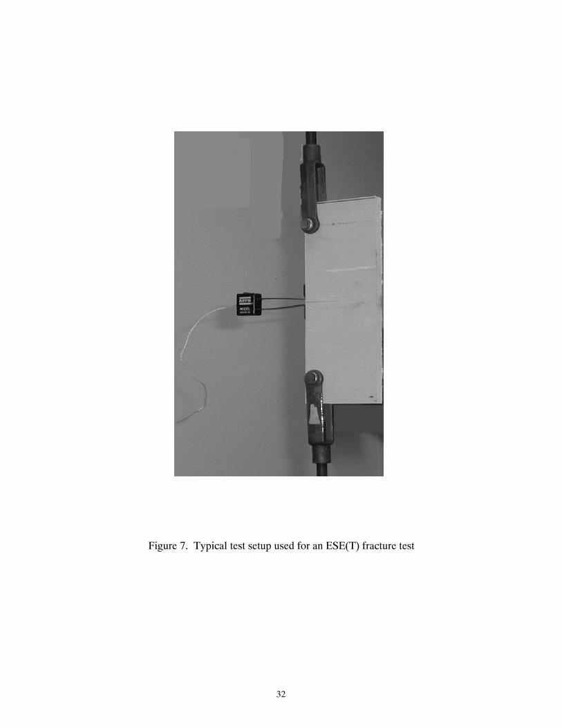
specimenwere also used to verify themodeling approach. The geometry of theESE(T) spec-
imen is shown in Figures 6 and 7. The load is applied through a pin clevis connected through
a threaded rod. The design allows the specimen to rotate freely in order to achieve a pin load-
ing condition. A clip gage attached to the specimen using knife edges is used in order tomea-
sure theNMOD. All tested specimenwere cut fromonemonolithic pultruded platewith 12.7
mm (0.5 in.) in thickness. The tests was performed in displacement control mode at a rate
of 1 mm/min. The load was applied using an MTS 810 servo--hydraulic test system with a
222.41 kN (50--kip) capacity. The accuracy of the recorded data is as follows: the load is
within 0.22 kN (50 lbf ) and the notch mouth opening displacement (NMOD) is within
3.3x10⁻² mm (1.3x10⁻³ in) .
Samples were sectioned and coated with a thin layer of gold using a sputter coater for
SEM fractography. The SEMmicrographs were taken after the fracture of an ESE(T) speci-
men with a∕W= 0.5. Figure 8 shows the fracture surface ahead of the notch tip in a region
with a roving bundle. The fiber in the roving bundle appear to be clear of the adheringmatrix.
Further a uniform fracture is seen in the CFM layer ahead of the notch. Figure 9 shows a
manufacturing defect (void) in the notch region area.
COHESIVE LAYER FRACTURE MODEL
Acohesive fracture type analysis combinedwith a nonlinear constitutivematerialmicro-
model is proposed to study the behavior before and after the onset of crack propagation. The

16
FE analysis was performed for all ESE(T) and SEN(T) specimen. A fracture surface (cohe-
sive layer) is introduced at the center and finely meshed with further refinement around the
notch tip. Uniform displacements are applied at the remote node where the resultant force
from the pin loading is assumed to act. The use of a specified crack path a priori is justified
because of self--similarmode--I crack growth. This is verified from repeated tests conducted
in this study. A linear traction separation law is used to simulate the creation of traction free
surfaces by ramping the nodal forces to zerowith continued loading. TheABAQUS implicit
finite element code is used with 4--node continuum plane strain elements (CPE4). A conver-
gence study was initially performed to determine an adequate mesh size. The ESE (T) aver-
agemodel size includes approximately 3000 elements and 3200 nodes. The SEN(T) average
model size is 4500 elements and 5000 nodes.
A traction based failure criterion is used to initiate the traction--separation failure criteri-
on for the crack growth process. The failure criterion for 2D fracturemodels includes normal
and shear stress components:
f = σnσfn 2+ τ1
τf1 2 (20)
where σn is the normal stress component, and τ1 is the shear stress. The normal and shear
stresses are σfn and τf1respectively. Only the normal stress contribution is considered for
the current mode of fracture. In addition to the failure criterion parameters, crack--growth
parameters are also needed. These are used to specify themanner inwhich the traction across
the failed interface is ramped to zero. The parameters of the traction separation curve are
a function of continued opening displacement or pseudo time. This can be correlated to the
apparent strain energy release rate. The parameters used in the calibration procedure for
crack growth are illustrated in Figure 2. The distance Lc from the crack tip is where the fail-
ure criterion is evaluated. The traction is reduced to zero as a function of the time after de-
bonding failure occurs. If the stresses are removed too rapidly, numerical convergence diffi-

17
culties may arise. The release time and the distance Lc are calibrated from one ESE(T)
load--NMOD experimental data for a ratio of a∕W= 0.5.
The experimental load--NMODused for this calibration is shown in Figure 10. The cohe-
sive normal failure stress, σfn is 82.7 MPa (12 ksi). It is chosen to have a close value to the
unnotched uniaxial tensile strength in the transverse direction. The time at which interface
tractions are ramped to zero when the criterion is met is tf = 0.03 (relative time in relation
to the total applied displacement at the end of the analysis, t = 1.0), and the distance from
the current crack tip at which the failure criterion is evaluated, Lc = 0.0028 mm (0.07 in).
The calibrated parameters for the cohesive model are used to predict the response and
crack growth of other ESE(T) geometries and crack sizes. This modeling approach was also
verified on a range of SEN(T) specimen.
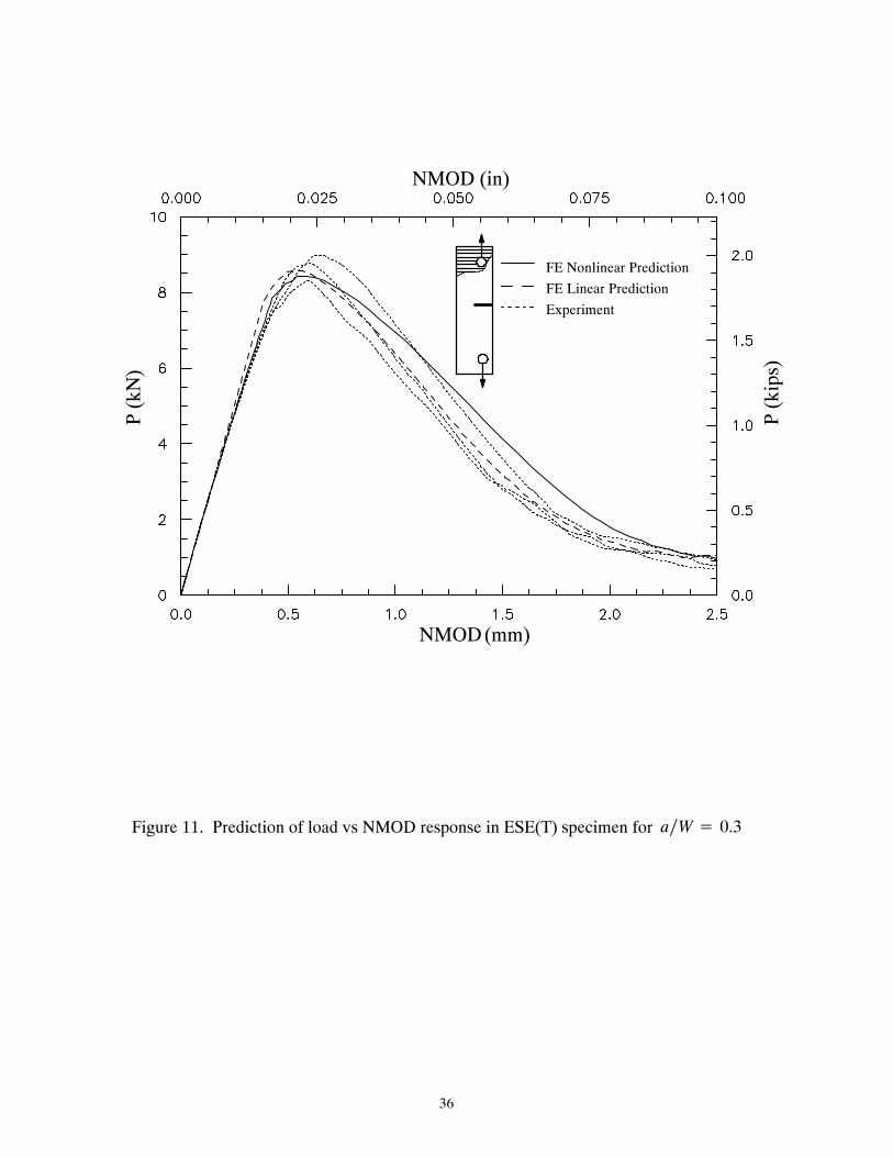
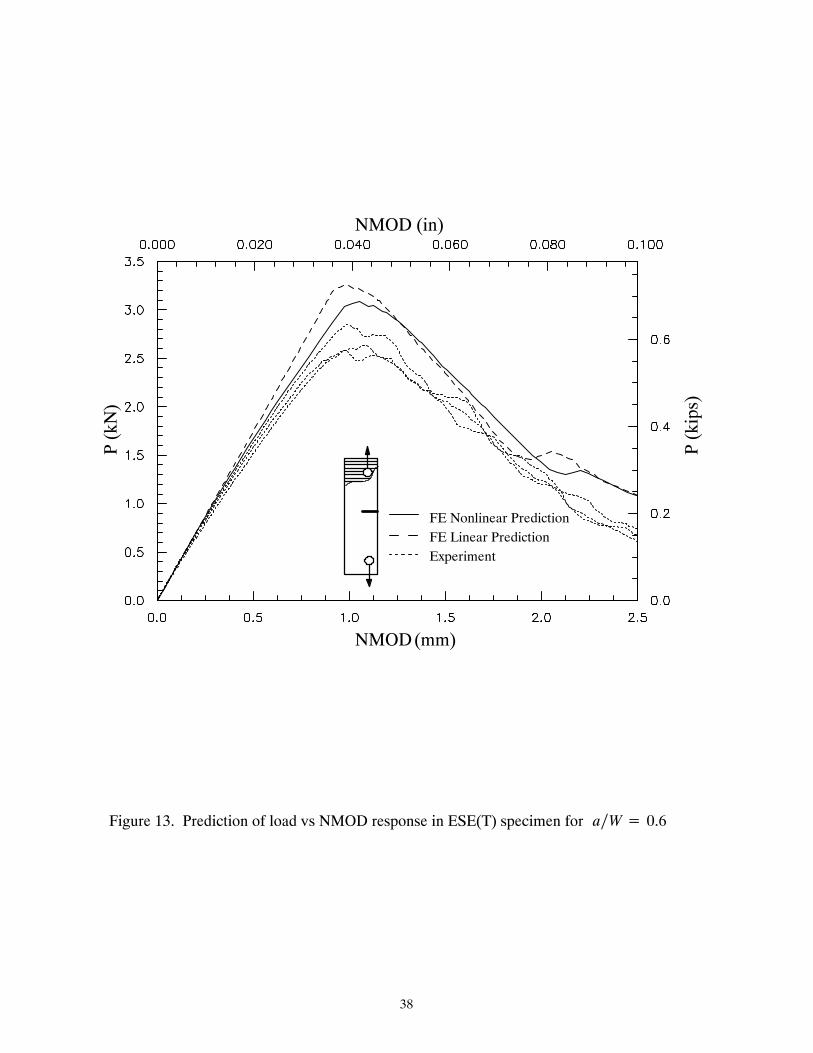
The predicted load--NMOD results from the nonlinear micromodels with the cohesive
FE are shown in Figures 11 -- 14 for ESE(T) specimen with a/W=0.3, 0.4, 0.6 and 0.7. The
initial effective linear and some nonlinear responses are captured by these analyses (The lin-
ear prediction is also plotted in Figure 5 to illustrate the nonlinearity effects). Good predic-
tion is demonstrated by the combined fracture modeling approach for all ESE(T) coupons.
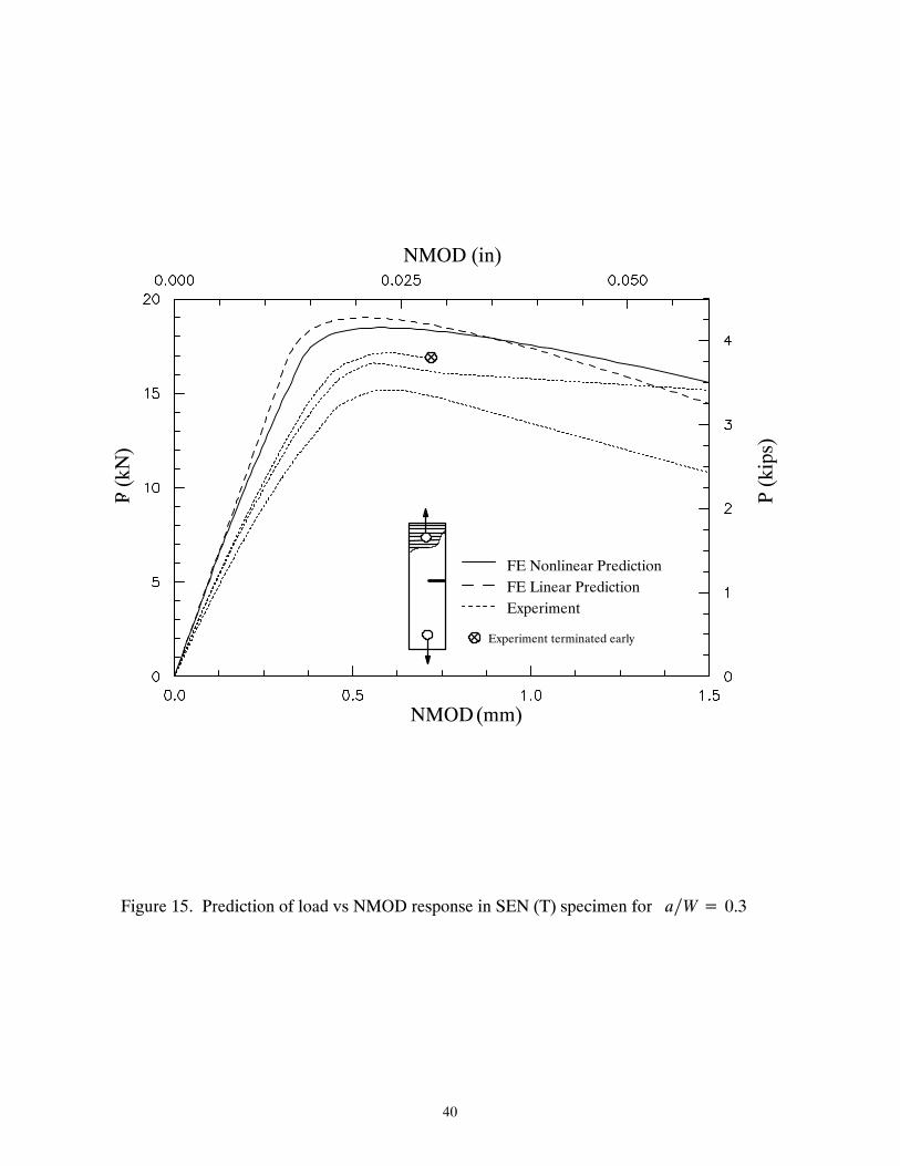
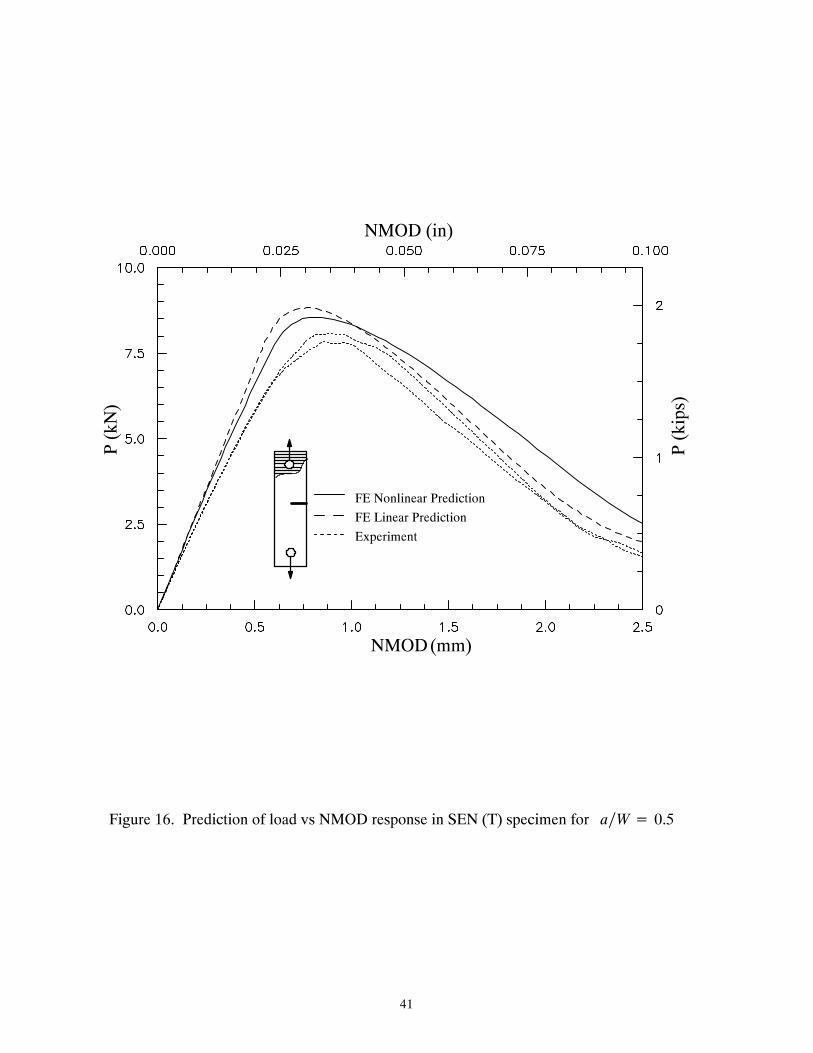
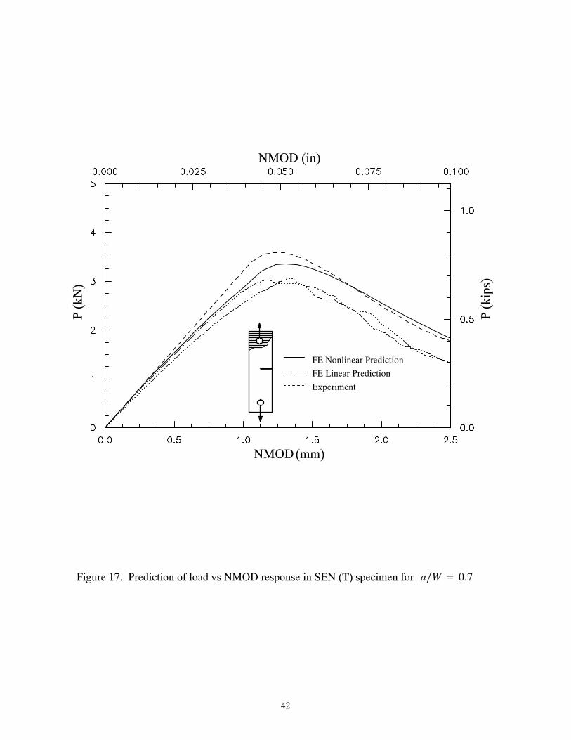
Figures 15 -- 17 show the predicted response for the SEN(T) fracture geometries. The same
calibrated parameters, from ESE(T) with a∕W= 0.5 are used in the SEN(T) case. Good
prediction is also shown for the SEN(T) fracture response. The predicted load--NMOD re-
sponse from the combined FE and the nonlinear micromodels better match the experimental
datawhen comparedwith the FEmodels with homogenized linear properties. The predicted
maximum loads from the nonlinearmodels are higher than the experimental data for the larg-
er a/W values. This may be attributed to an added softening from a larger damaged zone.
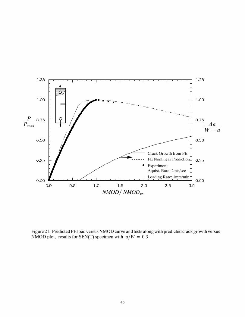
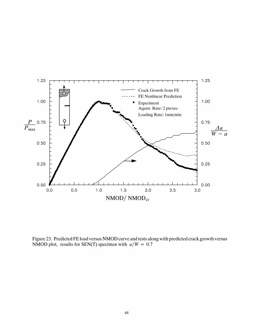
Crack growth data from the ESE(T) and SEN(T) models are extracted from the FE analysis
and plotted in Figures 18 -- 23. The NMOD is normalized by the NMOD at maximum load.
The crack growth curves are plotted on the right y--axis and the loading curves are plotted

18
on the left y--axiswith the common normalizedNMODon the x--axis. It is interesting to note
that some crack growth occurs before the maximum applied load, e.g. for ESE(T) and
SEN(T) with small a∕W= 0.3, Figures 18 and 21.
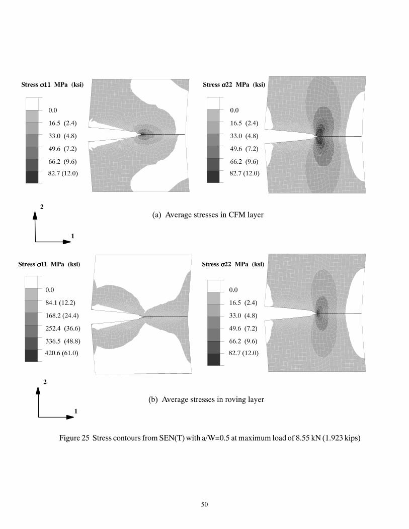
The combined use of micromechanical constitutive models allow plotting the average
deformations at the CFM and roving layers while monitoring the crack growth. Axial and
transverse stress contours are plotted for different loading levels for the roving andCFM lay-
ers. Figure 24 and 25 show the stresses in the homogenized roving and CFM layers for both
the ESE(T) and SEN(T) coupons, respectively. The stresses in the roving layers are not as
close to their ultimate strength value. Damage is more wide--spread in the CFM layers.
THERMOELASTIC STRESS ANALYSIS
A thermoelastic stress analysis (TSA) techniquewas used to confirm the fracturemodel-
ing in pultruded plates. Under adiabatic and reversible conditions in isotropicmaterials, the
application of a small cyclic loadwill induce small variations in temperature that are propor-
tional to the sum of principal stresses. In an in--plane transversely isotropic compositemate-
rial under plane stress conditions, the thermoelastic response is directly related to the sum
of the in--plane principal strain components. Therefore, the TSA method can be applied to
verify the stress singularity ahead of the notch and to compared with results from the FE
model in the linear range. ADeltaThermDT1500 thermoelasticitymeasurement systemwas
used to acquire the thermal measurements. The DeltaTherm’s infrared array detector syn-
chronized with the applied cyclical loading enables the detection of the thermoelastic effect
(change in stresses). The system has a thermal resolution of about 1 mK for image exposure
times of one minute or less (DeltaTherm 2001).
The tested coupons were coated with flat black paint to improve the surface emissivity.
The load was monotonically applied in 2.22 kN (0.5 kip) increments and held. During the
hold time of 5 minutes, a cyclic sinusoidal load was applied. The cyclic load had an ampli-
tude of 0.2 kips and a frequency of 6Hz. Data from the images were averaged by allowing

19
an exposure time of 5 minutes. Time effects during the hold period and for the cyclic load
applicationwere not considered significant because of thematerial effects and due to the sig-
nal integration that is synchronized only with the applied cyclic loading. This was verified
from the consistent ultimate load levels compared to those from fully static tests with no in-
terruptions. Direct temperature measurements were performed on another set of coupons
that were not interrupted with cyclic loadings. The exposure time was deemed not enough
for damage detection during the tests. The contour image from the TSA measurement is
shown in terms of camera relative units as shown in Figure 26. TSA results were compared
with FE predictions along the crack line in Figure 27. This shows that the normalized stress
curvesmergewith the singular stress field near the notch tip.While the objective of this study
is to model the propagating crack, achieving an exact singularity at the tip may not be crucial
since the fracture criterion is not localized and does not directly deal with the exact order of
the singularity.
CONCLUSIONS
Nonlinear 3D micromechanical models for pultruded composite materials are proposed
and used to analyze the fracture parallel to the roving direction in a polymeric matrix pul-
truded composite. The ESE (T) and SEN(T) geometries are modeled with these micromo-
dels and the results are compared from records of fracture toughness tests. Limited stable
crack propagation is shown to occur before attaining themaximum load. The proposed com-
bination of material and FE fracture models is capable of modeling crack progression. The
proposed models can also be used to study material and structural parameters that can affect
the fracture in pultruded composite materials and structures. The model can be extended to
study fracture when the load is applied at other angles to the roving direction.
The nature of production of this composite and the toughness in this direction derived
primarily from the resistance in the CFM layers. The proposed modeling framework is a
nestedmulti--scale approach that can include different micromodels for the layers within the

20
cross--section of the composite. This makes it a valuable tool in the prediction of other con-
figurations and layups of this material.
ACKNOWLEDGEMENT
This work was supported byNSF, through the Civil andMechanical Systems (CMS)Di-
vision, and under grant number 9876080.

21
REFERENCES
1. ABAQUS, Hibbitt, Karlsson and Sorensen, Inc. User’s Manual, Version 5.8, 1998.
2. ASTM E 1922, (1997), “Standard Test Method for Translaminar Fracture Toughness of
Laminated Polymer Matrix Composites.”, Annual Book of ASTM standards.
3. ASTMD 3039/D 3039M, (2000), “Standard Test Method for Tensile Properties of Poly-
mer Matrix Composite Materials.”, Annual Book of ASTM standards.
4. Christensen, R.M., andWaals, F. M., (1972), ‘‘Effective Stiffness of RandomlyOriented
Fibre Composites,“ J. Composite Materials, Vol. 6, pp. 518--532.
5. DeltaTherm Operation Manual, Stress Photonics Inc. Madison, WI, 2001.
6. Haj--Ali, R., M. and, Kilic, H., (2002a), In Press, ”Nonlinear Behavior of Pultruded FRP
composites,” Composites Journal Part B: Engineering.
7. Haj--Ali, R., M. and, Kilic, H., (2002b) ”Nonlinear Constitutive Models for Pultruded
FRP Composites, ” In press, Mechanics of Materials Journal.
8. Haj--Ali, R.M., and Pecknold, D.A., (1996), ‘‘ HierarchicalMaterialModels withMicro-
structure for Nonlinear Analysis of Progressive Damage in Laminated Composite Struc-
tures”, Structural Research Series No. 611, UILU--ENG--96--2007, Department of Civil En-
gineering, University of Illinois at Urbana--Champaign.
9. Holdsworth, A.W.,Owen,M. J.,Morris, S., (1974), “Macroscopic Fracture ofGlassRein-
forced Polyester Resin Laminates“, J. Composite Materials, Vol. 8, p. 177.
10. Kanninen, M. F., Rybicki, E. F., and Brinson, H. F., (1977a), “A Critical Look at current
applications of fracture mechanics to the failure of Fiber--Reinforced Composites,” Com-
posites, Vol. 8, pp. 17--22.

22
11. Kanninen, M. F., Rybicki, E. F., and Griffith,W. I., (1977b), “Preliminary Development
of a Fundamental AnalysisModel for Crack Growth in a Fiber Reinforced CompositeMate-
rial,”CompositeMaterials: Testing andDesign,ASTMSTP617,AmericanSociety forTest-
ing and Materials., pp. 53--69.
12. Konish, H. J., Swedlow, J. L., and Cruse, T. A., (1972), “Experimental Investigation of
Fracture in an Advanced Fiber Composite,” J. of Comp. Mat., 6, pp. 114--124.
13. Konish Jr., H. J., Swedlow, J. L., Cruse, T.A.,(1973), ”Fracture Phenomena inAdvanced
Fiber Composite Materials”, AIAA Journal, Vol.11, No. 3, pp.40--43.
14. Mandell, J. F.,McGarry, F. J.,Wang, S. S., and Im, J., “Stress Intensity Factors forAniso-
tropic Fracture Test Specimens of Several Geometries,” J. of Comp. Mat., 8, pp. 106--116.
15. Pagano, N. J., (1974), ”Exact Moduli of Anisotropic Laminates,” Mechanics of Com-
posite Materials, Sendeckyj, G. P., (Ed.), Academic Press, pp. 23--44.
16. Parhizgar, S., Zachary, L. W., and Sun, C. T., (1982), “Application of the Principles of
Linear Fracture Mechanics to the Composite Materials,” International Journal of Fracture,
20, pp. 3--15.
17. Sih. G. C., Chen, E. P., Huang, S. L., and,McQuillen, E. J., (1975), “Material Character-
ization on the Fracture of Filament Reinforced Composites,” J. of CompositeMaterials, Vol.
9, pp. 167--186.
18. Sih, G. C., Paris, P. C., Irwin, G. R., (1965), “On Cracks in Rectilinearly Anisotropic
Bodies”, International Journal of Fracture Mechanics, Vol. 1, No.3, pp. 189--203.
19. Tsai, S., W., Pagano, N. J., “Invariant Properties of Composite Materials,” Composite
Materials Workshop, Technomic Publishing Co., 1968.
20. Waddoups, E.M., Eisenmann, J. R., and Kaminiski, B. E., (1971), “Macroscopic Frac-

23
tureMecchanics of Advanced CompositeMaterials.” J. CompositeMaterials, Vol. 5, p. 446.

24
E ν
Fiber (E--glass)
Matrix(Polyester + Fillers)
10500 0.25
0.30
(ksi)β τon
(ksi)
630 4.0 6.02.0
Table 1. Elastic properties and matrix nonlinear Ramberg--Osgood parameters,fiber volume fraction in: roving layers = 0.407 , CFM layers = 0.305
-- -- --

25
Micromodel
E1 ν13
Experimental 2.484
0.295
E2(Msi)
ν23G12
1.444 0.507
2.730 1.641 0.609 0.319
E3
1.130
G13
0.377
G23
0.357
ν12
0.273
2.627 1.582(--)(+)
Table 2. Predicted and experimental cross--section elastic properties
0.2830.291Experimental 0.520--
------
----
----
----

26
Figure 1. Cross--sectional view transverse to the unidirectional roving in a pultruded composite plate
12.7mm(0.5in)
Roving Layer
CFM Layer
Protective Veil
(b) Sectioned coupon cut across the thickness
(a) Side view
Roving Layers
CFM Layer

27
Multi ---Scale 3D Modelfor Pultruded Composites
Roving
CFM
3
2
Roving Unit Cell ModelCFM Unit Cell Model
fiberbundles
IdealizedRoving Layer
fiber
fiber
(1) (1)
fiber
matrix
matrix
matrixmatrix
matrix
(3) (3)(4)
(2) (2)
(4)
ε
σ
ε
σ
ε
σ
fibermatrixfibermatrix
1− h
1− b
h
b1 1
h 1− h
1− b
b
ε
σ
ξb
MaterialPoint
2D---Finite Element
X2
X3
X1orX2
X3
Figure 2. A framework for 3D nonlinear analysis of pultruded composite structures.
tft − tcr
1
00
T/Tcr
Cohesive Layer Parameters
IdealizedCFM Layer
Structural or Component Level
Predeterminedcrack path

28
Angle, °0
Exx
(ksi)
Exx
(MPa)
Micromodel Prediction12.7 mm (1/2”) compression coupons12.7 mm (1/2”) tension coupons
Figure 3. Prediction of off--axis elastic stiffness of coupons in tension and compression.
°

29
Strain, ⁄ (%)
Stress,″(M
Pa)
Stress,″
(ksi)
°
MicromodelCalibration
Linear Prediction
Tension Tests
Compression Test
Figure 4. Calibration of nonlinear behavior from transverse coupons in tension and compression (°= 900)
TensionTests
Micromodel(Calibration)
CompressionTest
Micromodel (Linear)

30
Strain, ⁄ (%)
Stress,″(M
Pa)
Stress,″
(ksi)
MicromodelPrediction
Tension Tests
Figure 5. Axial stress--strain response for different E--glass/polyester off--axis tests
θ= 0o
θ= 15o
θ= 30o
θ= 45o
θ= 60o
°

31
6.35 mm (0.5”) Dia.
63.5 mm (2.5”)
254mm(10”)
31.7mm(1.25”)
Notch Length(Varies)
Pin LoadingClevis
AttachedKnife Edges
Clip Gage toMeasure NMOD
Figure 6. ESE(T) test specimen and experimental setup
12.7mm (0.5”)
32
Figure 7. Typical test setup used for an ESE(T) fracture test

33
Notch Tip
Roving Bundle
Figure 8. Roving area ahead of the notch tip

34
Voids
Notch Tip
Roving Bundle
Figure 9. Manufacturing defect (void) in the notch region

35
Figure 10. Load vs. NMOD used for calibration of cohesive layer parameters fromESE(T) specimen for a∕W= 0.5
NMOD(mm)
NMOD (in)
P(kN)
P(kips)
FE Nonlinear CalibrationFE Linear PredictionExperiment
36
Figure 11. Prediction of load vs NMOD response in ESE(T) specimen for a∕W= 0.3
NMOD(mm)
NMOD (in)
P(kN)
P(kips)
FE Nonlinear PredictionFE Linear PredictionExperiment

37
Figure 12. Prediction of Load vs NMOD response in ESE(T) specimen for a∕W= 0.4
NMOD(mm)
NMOD (in)
P(kN)
P(kips)
FE Nonlinear PredictionFE Linear PredictionExperiment
38
Figure 13. Prediction of load vs NMOD response in ESE(T) specimen for a∕W= 0.6
NMOD(mm)
NMOD (in)
P(kN)
P(kips)
FE Nonlinear PredictionFE Linear PredictionExperiment

39
Figure 14. Prediction of load vs NMOD response in ESE(T) specimen for a∕W= 0.7
NMOD(mm)
NMOD (in)
P(kN)
P(kips)
FE Nonlinear PredictionFE Linear PredictionExperiment
40
Figure 15. Prediction of load vs NMOD response in SEN (T) specimen for a∕W= 0.3
NMOD(mm)
NMOD (in)
P(kN)
P(kips)
FE Nonlinear PredictionFE Linear PredictionExperiment
Experiment terminated early
41
Figure 16. Prediction of load vs NMOD response in SEN (T) specimen for a∕W= 0.5
NMOD(mm)
NMOD (in)
P(kN)
P(kips)
FE Nonlinear PredictionFE Linear PredictionExperiment
42
Figure 17. Prediction of load vs NMOD response in SEN (T) specimen for a∕W= 0.7
NMOD(mm)
NMOD (in)
P(kN)
P(kips)
FE Nonlinear PredictionFE Linear PredictionExperiment

43
Figure 18. PredictedFE load versusNMODcurve and tests alongwith predicted crack growth versusNMOD plot, results for ESE(T) specimen with a∕W= 0.3
NMOD∕ NMODcr
∆aW− a
PPmax
FE Nonlinear Prediction
Experiment
Crack Growth from FE
Aquist. Rate: 2 pts/secLoading Rate: 1mm/min

44
Figure 19. PredictedFE load versusNMODcurve and tests alongwith predicted crack growth versusNMOD plot, results for ESE(T) specimen with a∕W= 0.5
NMOD∕ NMODcr
∆aW− a
PPmax
FE Nonlinear Prediction
Experiment
Crack Growth from FE
Aquist. Rate: 2 pts/secLoading Rate: 1mm/min

45
Figure 20. PredictedFE load versusNMODcurve and tests alongwith predicted crack growth versusNMOD plot, results for ESE(T) specimen with a∕W= 0.7
NMOD∕ NMODcr
∆aW− a
PPmax
FE Nonlinear Prediction
Experiment
Crack Growth from FE
Aquist. Rate: 2 pts/secLoading Rate: 1mm/min
46
Figure 21. PredictedFE load versusNMODcurve and tests alongwith predicted crack growth versusNMOD plot, results for SEN(T) specimen with a∕W= 0.3
NMOD∕ NMODcr
∆aW− a
PPmax
FE Nonlinear Prediction
Experiment
Crack Growth from FE
Aquist. Rate: 2 pts/secLoading Rate: 1mm/min
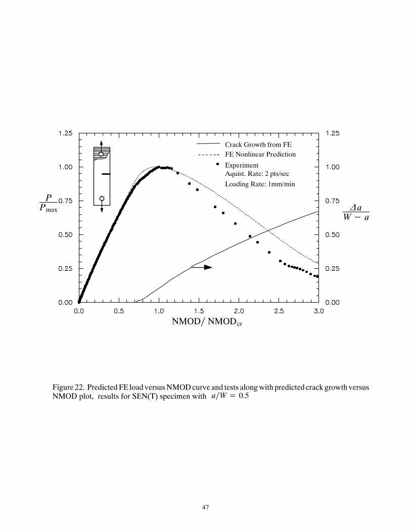
47
Figure 22. PredictedFE load versusNMODcurve and tests alongwith predicted crack growth versusNMOD plot, results for SEN(T) specimen with a∕W= 0.5
NMOD∕ NMODcr
∆aW− a
PPmax
FE Nonlinear Prediction
Experiment
Crack Growth from FE
Aquist. Rate: 2 pts/secLoading Rate: 1mm/min
48
Figure 23. PredictedFE load versusNMODcurve and tests alongwith predicted crack growth versusNMOD plot, results for SEN(T) specimen with a∕W= 0.7
NMOD∕ NMODcr
∆aW− a
PPmax
FE Nonlinear Prediction
Experiment
Crack Growth from FE
Aquist. Rate: 2 pts/secLoading Rate: 1mm/min

49
0.0
16.5 (2.4)
33.0 (4.8)
49.6 (7.2)
66.2 (9.6)
82.7 (12.0)
Stress ″″″″ΝΝΝΝΝΝΝΝ MPa (ksi)
0.0
16.5 (2.4)
33.0 (4.8)
49.6 (7.2)
66.2 (9.6)
82.7 (12.0)
Stress ″″″″22 MPa (ksi)
0.0
16.5 (2.4)
33.0 (4.8)
49.6 (7.2)
66.2 (9.6)
82.7 (12.0)
Stress ″″″″22 MPa (ksi)
0.0
84.1 (12.2)
168.2 (24.4)
252.4 (36.6)
336.5 (48.8)
420.6 (61.0)
Stress ″″″″11 MPa (ksi)
(a) Average stresses in CFM layer
(b) Average Stresses in roving layer
Figure 24 Axial and transverse stress contours from ESE(T) with a/W=0.5 at maximum loadof 4.32 kN (0.971 kips)
2
1
2
1
50
0.0
16.5 (2.4)
33.0 (4.8)
49.6 (7.2)
66.2 (9.6)
82.7 (12.0)
Stress ″″″″ΝΝΝΝΝΝΝΝ MPa (ksi)
0.0
16.5 (2.4)
33.0 (4.8)
49.6 (7.2)
66.2 (9.6)
82.7 (12.0)
Stress ″″″″22 MPa (ksi)
0.0
16.5 (2.4)
33.0 (4.8)
49.6 (7.2)
66.2 (9.6)
82.7 (12.0)
Stress ″″″″22 MPa (ksi)
0.0
84.1 (12.2)
168.2 (24.4)
252.4 (36.6)
336.5 (48.8)
420.6 (61.0)
Stress ″″″″11 MPa (ksi)
(a) Average stresses in CFM layer
(b) Average stresses in roving layer
Figure 25 Stress contours from SEN(T) with a/W=0.5 at maximum load of 8.55 kN (1.923 kips)
2
1
2
1

51
Figure 26. TSA image of SEN(T) speciemen with a∕W= 0.3
Pultruded Single Edge Notch SpecimenLoad Level = 2.22 ± 0.89 kN (0.5 ±0.2 kips)Frequency = 6 Hz
--838.
--859.
667.
1419.
2171.
2923.
5180.
8189.
TSA Signal

52
Distance from the Notch Tip, mm
Distance from the Notch Tip, in
NormalizedStress(TSASignal) NormalizedOpening Stress fromFE
Normalized TSA Signal
Figure 27. Verification of stress pattern from TSA and FE on SEN(T) speciemen with
TSA test with::Load = 0.6 kips with amplitude = 0.2 kips
a∕W= 0.3
Related Documents