Cosmology from string theory

arX

iv:0

704.

0928

v3 [

hep-

ph]

26

Oct

200

7

Cosmology from String Theory

Luis Anchordoqui,1 Haim Goldberg,2 Satoshi Nawata,1 and Carlos Nunez3

1Department of Physics,

University of Wisconsin-Milwaukee, Milwaukee, WI 53201

2Department of Physics,

Northeastern University, Boston, MA 02115

3 Department of Physics,

University of Swansea, Singleton Park, Swansea SA2 8PP, UK

(Dated: April 2007)

AbstractWe explore the cosmological content of Salam-Sezgin six dimensional supergravity, and find a

solution to the field equations in qualitative agreement with observation of distant supernovae,

primordial nucleosynthesis abundances, and recent measurements of the cosmic microwave back-

ground. The carrier of the acceleration in the present de Sitter epoch is a quintessence field slowly

rolling down its exponential potential. Intrinsic to this model is a second modulus which is au-

tomatically stabilized and acts as a source of cold dark matter, with a mass proportional to an

exponential function of the quintessence field (hence realizing VAMP models within a String con-

text). However, any attempt to saturate the present cold dark matter component in this manner

leads to unacceptable deviations from cosmological data – a numerical study reveals that this

source can account for up to about 7% of the total cold dark matter budget. We also show that

(1) the model will support a de Sitter energy in agreement with observation at the expense of a

miniscule breaking of supersymmetry in the compact space; (2) variations in the fine structure

constant are controlled by the stabilized modulus and are negligible; (3) “fifth” forces are carried

by the stabilized modulus and are short range; (4) the long time behavior of the model in four

dimensions is that of a Robertson-Walker universe with a constant expansion rate (w = −1/3).

Finally, we present a String theory background by lifting our six dimensional cosmological solution

to ten dimensions.

1

I. GENERAL IDEA

The mechanism involved in generating a very small cosmological constant that satisfies’t Hooft naturalness is one of the most pressing questions in contemporary physics. Re-cent observations of distant Type Ia supernovae [1] strongly indicate that the universe isexpanding in an accelerating phase, with an effective de-Sitter (dS) constant H that nearlysaturates the upper bound given by the present-day value of the Hubble constant, i.e.,H <∼ H0 ∼ 10−33 eV. According to the Einstein field equations, H provides a measure ofthe scalar curvature of the space and is related to the vacuum energy density ρvac throughFriedmann’s equation, 3 M2

PlH2 ∼ ρvac, where MPl ≃ 2.4 × 1018 GeV is the reduced Planck

mass. However, the “natural” value of ρvac coming from the zero-point energies of knownelementary particles is found to be at least ρvac ∼ TeV4. Substitution of this value of ρvac intoFriedmann’s equation yields H >∼ 10−3 eV, grossly inconsistent with the set of supernova(SN) observations. The absence of a mechanism in agreement with ’t Hooft naturalnesscriteria then centers on the following question: why is the vacuum energy needed by theEinstein field equations 120 orders of magnitude smaller than any “natural” cut-off scale ineffective field theory of particle interactions, but not zero?

Nowadays, the most popular framework which can address aspects of this question isthe anthropic approach, in which the fundamental constants are not determined throughfundamental reasons, but rather because such values are necessary for life (and hence intel-ligent observers to measure the constants) [2]. Of course, in order to implement this idea ina concrete physical theory, it is necessary to postulate a multiverse in which fundamentalphysical parameters can take different values. Recent investigations in String theory haveapplied a statistical approach to the enormous “landscape” of metastable vacua present inthe theory [3]. A vast ensemble of metastable vacua with a small positive effective cosmo-logical constant that can accommodate the low energy effective field theory of the StandardModel (SM) have been found. Therefore, the idea of a string landscape has been used toproposed a concrete implementation of the anthropic principle.

Nevertheless, the compactification of a String/M-theory background to a four dimen-sional solution undergoing accelerating expansion has proved to be exceedingly difficult.The obstruction to finding dS solutions in the low energy equations of String/M theoryis well known and summarized in the no-go theorem of [4]. This theorem states that ina D-dimensional theory of gravity, in which (a) the action is linear in the Ricci scalarcurvature (b) the potential for the matter fields is non-positive and (c) the massless fieldshave positive defined kinetic terms, there are no (dynamical) compactifications of the form:ds2

D = Ω2(y)(dx2d+ gmndyndym), if the d dimensional space has Minkowski SO(1, d−1) or dS

SO(1, d) isometries and its d dimensional gravitational constant is finite (i.e., the internalspace has finite volume). The conclusions of the theorem can be circumvented if some of itshypotheses are not satisfied. Examples where the hypotheses can be relaxed exist: (i) onecan find solutions in which not all of the internal dimensions are compact [5]; (ii) one maytry to find a solution breaking Minkowski or de Sitter invariance [6]; (iii) one may try toadd negative tension matter (e.g., in the form of orientifold planes) [7]; (iv) one can evenappeal to some intrincate String dynamics [8].

Salam-Sezgin six dimensional supergravity model [9] provides a specific example wherethe no-go theorem is not at work, because when their model is lifted to M theory theinternal space is found to be non-compact [10]. The lower dimensional perspective of this,is that in six dimensions the potential can be positive. This model has perhaps attracted

2

the most attention because of the wide range of its phenomenological applications [11]. Inthis article we examine the cosmological implications of such a supergravity model duringthe epochs subsequent to primordial nucleosynthesis. We derive a solution of Einstein fieldequations which is in qualitative agreement with luminosity distance measurements of TypeIa supernovae [1], primordial nucleosynthesis abundances [12], data from the Sloan DigitalSky Survey (SDSS) [13], and the most recent measurements from the Wilkinson MicrowaveAnisotropy Probe (WMAP) satellite [14]. The observed acceleration of the universe isdriven by the “dark energy” associated to a scalar field slowly rolling down its exponentialpotential (i.e., kinetic energy density < potential energy density ≡ negative pressure) [15].Very interestingly, the resulting cosmological model also predicts a cold dark matter (CDM)candidate. In analogy with the phenomenological proposal of [16], such a nonbaryonic matterinteracts with the dark energy field and therefore the mass of the CDM particles evolves withthe exponential dark energy potential. However, an attempt to saturate the present CDMcomponent in this manner leads to gross deviations from present cosmological data. Wewill show that this type of CDM can account for up to about 7% of the total CDM budget.Generalizations of our scenario (using supergravities with more fields) might account for therest.

II. SALAM-SEZGIN COSMOLOGY

We begin with the action of Salam-Sezgin six dimensional supergravity [9], setting tozero the fermionic terms in the background (of course fermionic excitations will arise fromfluctuations),

S =1

4κ2

∫d6x

√g6

[R − κ2(∂Mσ)2 − κ2eκσF 2

MN − 2g2

κ2e−κσ − κ2

3e2κσG2

MNP

]. (1)

Here, g6 = det gMN , R is the Ricci scalar of gMN , FMN = ∂[MAN ], GMNP = ∂[MBNP ] +κA[MFNP ], and capital Latin indices run from 0 to 5. A re-scaling of the constants: G6 ≡ 2κ2,φ ≡ −κσ and ξ ≡ 4 g2 leads to

S =1

2G6

∫d6x

√g6

[R − (∂Mφ)2 − ξ

G6

eφ − G6

2e−φF 2

MN − G6

6e−2φG2

MNP

]. (2)

The length dimensions of the fields are: [G6] = L4, [ξ] = L2, [φ] = [g2MN ] = 1, [A2

M ] = L−4,and [F 2

MN ] = [G2MNP ] = L−6.

Now, we consider a spontaneous compactification from six dimension to four dimension.To this end, we take the six dimensional manifold M to be a direct product of 4 Minkowskidirections (hereafter denoted by N1) and a compact orientable two dimensional manifold N2

with constant curvature. Without loss of generality, we can set N2 to be a sphere S2, or aΣ2 hyperbolic manifold with arbitrary genus. The metric on M locally takes the form

ds26 = ds4(t, ~x)2 + e2f(t,~x)dσ2, dσ2 =

r2c (dϑ2 + sin2 ϑdϕ2) for S2

r2c (dϑ2 + sinh2 ϑdϕ2) for Σ2 ,

(3)

where (t, ~x) denotes a local coordinate system in N1, rc is the compactification radius of N2.We assume that the scalar field φ is only dependent on the point of N1, i.e., φ = φ(t, ~x).We further assume that the gauge field AM is excited on N2 and is of the form

Aϕ =

b cos ϑ (S2)b cosh ϑ (Σ2) .

(4)

3

This is the monopole configuration detailed by Salam-Sezgin [9]. Since we set the Kalb-Ramond field BNP = 0 and the term A[MFNP ] vanishes on N2, GMNP = 0. The fieldstrength becomes

F 2MN = 2b2e−4f/r4

c . (5)

Taking the variation of the gauge field AM in Eq. (2) we obtain the Maxwell equation

∂M

[√g4√

gσe2f−φF MN

]= 0. (6)

It is easily seen that the field strengths in Eq. (5) satisfy Eq. (6).With this in mind, the Ricci scalar reduces to [17]

R[M ] = R[N1] + e−2fR[N2] − 42f − 6(∂µf)2 , (7)

where R[M ], R[N1], and R[N2] denote the Ricci scalars of the manifolds M, N1, and N2;respectively. (Greek indices run from 0 to 3). The Ricci scalar of N2 reads

R[N2] =

+2/r2

c (S2)−2/r2

c (Σ2).(8)

To simplify the notation, from now on, R1 and R2 indicate R[N1] and R[N2], respectively.The determinant of the metric can be written as

√g6 = e2f√g4

√gσ, where g4 = det gµν and

gσ is the determinant of the metric of N2 excluding the factor e2f . We define the gravitationalconstant in the four dimension as

1

G4≡ M2

Pl

2=

1

2 G6

∫d2σ

√gσ =

2πr2c

G6. (9)

Hence, by using the field configuration given in Eq. (4) we can re-write the action in Eq. (2)as follows

S =1

G4

∫d4x

√g4

e2f [R1 + e−2fR2 + 2(∂µf)2 − (∂µφ)2] − ξ

G6

e2f+φ − G6b2

r4c

e−2f−φ

. (10)

Let us consider now a rescaling of the metric of N1: gµν ≡ e2fgµν and√

g4 = e4f√g4. Such atransformation brings the theory into the Einstein conformal frame where the action givenin Eq. (10) takes the form

S =1

G4

∫d4x

√g4

[R[g4] − 4(∂µf)2 − (∂µφ)2 − ξ

G6e−2f+φ − G6b

2

r4c

e−6f−φ + e−4fR2

]. (11)

The four dimensional Lagrangian is then

L =

√g

G4

[R − 4(∂µf)2 − (∂µφ)2 − V (f, φ)

], (12)

with

V (f, φ) ≡ ξ

G6

e−2f+φ +G6b

2

r4c

e−6f−φ − e−4fR2 , (13)

where to simplify the notation we have defined: g ≡ g4 and R ≡ R[g4].

4

Let us now define a new orthogonal basis, X ≡ (φ + 2f)/√

G4 and Y ≡ (φ − 2f)/√

G4,so that the kinetic energy terms in the Lagrangian are both canonical, i.e.,

L =√

g[

R

G4

− 1

2(∂X)2 − 1

2(∂Y )2 − V (X, Y )

], (14)

where the potential V (X, Y ) ≡ V (f, φ)/G4 can be re-written (after some elementary algebra)as [18]

V (X, Y ) =e√

G4Y

G4

[G6b

2

r4c

e−2√

G4X − R2e−√

G4X +ξ

G6

]. (15)

The field equations are

Rµν −1

2gµνR =

G4

2

[(∂µX∂νX − gµν

2∂ηX ∂ηX

)

+(∂µY ∂νY − gµν

2∂ηY ∂ηY

)− gµνV (X, Y )

], (16)

2X = ∂X V , and 2Y = ∂Y V . In order to allow for a dS era we assume that the metric takesthe form

ds2 = −dt2 + e2h(t)d~x 2, (17)

and that X and Y depend only on the time coordinate, i.e., X = X(t) and Y = Y (t). Thenthe equations of motion for X and Y can be written as

X + 3hX = −∂X V (18)

andY + 3hY = −∂Y V , (19)

whereas the only two independent components of Eq. (16) are

h2 =G4

6

[1

2(X2 + Y 2) + V (X, Y )

](20)

and

2h + 3h2 =G4

2

[−1

2(X2 + Y 2) + V (X, Y )

]. (21)

The terms in the square brackets in Eq. (15) take the form of a quadratic function of

e−√

G4 X . This function has a global minimum at e−√

G4 X0 = R2 r4c/(2 G6 b2). Indeed, the

necessary and sufficient condition for a minimum is that R2 > 0, so hereafter we onlyconsider the spherical compactification, where e−

√G4 X0 = M2

Pl/(4πb2). The condition forthe potential to show a dS rather than an AdS or Minkowski phase is ξb2 > 1. Now, weexpand Eq. (15) around the minimum,

V (X, Y ) =e√

G4 Y

G4

K +

MX2

2(X − X0)

2 + O((X − X0)

3) , (22)

where

MX ≡ 1√π brc

(23)

5

and

K ≡ M2Pl

4πr2cb

2(b2ξ − 1) . (24)

As shown by Salam-Sezgin [9] the requirements for preserving a fraction of supersymmetry(SUSY) in spherical compactifications to four dimension imply b2ξ = 1, corresponding towinding number n = ±1 for the monopole configuration. Consequently, a (Y -dependent)dS background can be obtained only through SUSY breaking. For now we will leave openthe symmetry breaking mechanism and come back to this point after our phenomenologicaldiscussion. The Y -dependent physical mass of the X-particles at any time is

MX(Y ) =e√

G4 Y/2

√G4

MX , (25)

which makes this a varying mass particle (VAMP) model [16], although, in this case, thedependence on the quintessence field is fixed by the theory. The dS (vacuum) potentialenergy density is

VY =e√

G4 Y

G4K . (26)

In general, classical oscillations for the X particle will occur for

MX > H =

√G4ρtot

3, (27)

where ρtot is the total energy density. (This condition is well known from axion cosmol-ogy [19]). A necessary condition for this to hold can be obtained by saturating ρ with VY

from Eq. (26) and making use of Eqs. (23) to (27), which leads to ξb2 < 7. Of course, aswe stray from the present into an era where the dS energy is not dominant, we must checkat every step whether the inequality (27) holds. If the inequality is violated, the X-particleceases to behave like CDM.

In what follows, some combination of the parameters of the model will be determined byfitting present cosmological data. To this end we assume that SM fields are confined to N1

and we denote with ρrad the radiation energy, with ρX the matter energy associated withthe X-particles, and with ρmat the remaining matter density. With this in mind, Eq. (19)can be re-written as

Y + 3 H Y = −∂Veff

∂Y, (28)

where Veff ≡ VY + ρX and H is defined by the Friedmann equation

H2 ≡ h2 =1

3M2Pl

[1

2Y 2 + Veff + ρrad + ρmat

]. (29)

(Note that the matter energy associated to the X particles is contained in Veff .)It is more convenient to consider the evolution in u ≡ − ln(1 + z), where z is the redshift

parameter. As long as the oscillation condition is fulfilled, the VAMP CDM energy densityis given in terms of the X-particle number density nX [20]

ρX(Y, u) = MX(Y ) nX(u) = C e√

G4Y/2 e−3u , (30)

6

where C is a constant to be determined by fitting to data. Along with Eq. (26), these definefor us the effective (u-dependent) VAMP potential

Veff(Y, u) ≡ VY + ρX = A e√

G4Y + C e√

G4Y/2 e−3u , (31)

where a A is just a constant given in terms of model parameters through Eqs. (22) and (24).Hereafter we adopt natural units, MPl = 1. Denoting by a prime derivatives with respect

to u, the equation of motion for Y becomes

Y ′′

1 − Y ′2/6+ 3 Y ′ +

∂uρ Y ′/2 + 3 ∂Y Veff

ρ= 0 , (32)

where ρ = Veff + ρrad + ρmat. Quantities of importance are the dark energy density

ρY =1

2H2 Y ′2 + VY , (33)

generally expressed in units of the critical density (Ω ≡ ρ/ρc)

ΩY =ρY

3H2, (34)

and the Hubble parameter

H2 =ρ

3 − Y ′2/2. (35)

The equation of state is

wY =

[H2 Y ′2

2− VY

] [H2 Y ′2

2+ VY

]−1

. (36)

We pause to note that the exponential potential VY ∼ eλY/MPl , with λ =√

2. Asymptotically,this represents the crossover situation with wY = −1/3 [22], implying expansion at constantvelocity. Nevertheless, we will find that there is a brief period encompassing the recent past(z <∼ 6) where there has been significant acceleration.

Returning now to the quantitative analysis, we take ρmat = Be−3u and ρrad =10−4 ρmat e−u f(u) [21] where B is a constant and f(u) parameterizes the u-dependentnumber of radiation degrees of freedom. In order to interpolate the various thresholdsappearing prior to recombination (among others, QCD and electroweak), we adopt a conve-nient phenomenological form f(u) = exp(−u/15) [23]. We note at this point that solutionsof Eq. (32) are independent by an overall normalization for the energy density. This is alsotrue for the dimensionless quantities of interest ΩY and wY .

With these forms for the energy densities, Eq. (32) can be integrated for various choicesof A, B, and C, and initial conditions at u = −30. We take as initial condition Y (−30) = 0.Because of the slow variation of Y over the range of u, changes in Y (−30) are equivalentto altering the quantities A and C [24]. In accordance to equipartition arguments [24, 25]we take Y ′(−30) = 0.08. Because the Y evolution equation depends only on energy densityratios, and hence only on the ratios A : B : C of the previously introduced constants, wemay, for the purposes of integration and without loss of generality, arbitrarily fix B andthen scan the A and C parameter space for applicable solutions. In Fig. 1 we show a samplequalitative fit to the data. It has the property of allowing the maximum value of X-CDM

7

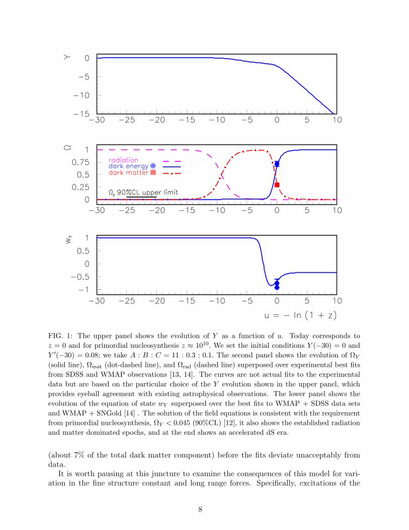
FIG. 1: The upper panel shows the evolution of Y as a function of u. Today corresponds to

z = 0 and for primordial nucleosynthesis z ≈ 1010. We set the initial conditions Y (−30) = 0 and

Y ′(−30) = 0.08; we take A : B : C = 11 : 0.3 : 0.1. The second panel shows the evolution of ΩY

(solid line), Ωmat (dot-dashed line), and Ωrad (dashed line) superposed over experimental best fits

from SDSS and WMAP observations [13, 14]. The curves are not actual fits to the experimental

data but are based on the particular choice of the Y evolution shown in the upper panel, which

provides eyeball agreement with existing astrophysical observations. The lower panel shows the

evolution of the equation of state wY superposed over the best fits to WMAP + SDSS data sets

and WMAP + SNGold [14] . The solution of the field equations is consistent with the requirement

from primordial nucleosynthesis, ΩY < 0.045 (90%CL) [12], it also shows the established radiation

and matter dominated epochs, and at the end shows an accelerated dS era.

(about 7% of the total dark matter component) before the fits deviate unacceptably fromdata.

It is worth pausing at this juncture to examine the consequences of this model for vari-ation in the fine structure constant and long range forces. Specifically, excitations of the

8

electromagnetic field on N1 will, through the presence of the dilaton factor in Eq. (2), seem-ingly induce variation in the electromagnetic fine structure constant αem = e2/4π, as wellas a violation of the equivalence principle through a long range coupling of the dilaton tothe electromagnetic component of the stress tensor. We now show that these effects areextremely negligible in the present model. First, it is easily seen using Eqs. (2) and (3)together with Eqs. (8)-(15), that the electromagnetic piece of the lagrangian as viewed fromN1 is

Lem = −2π

4e−

√G4X f 2

µν , (37)

where fµν denotes a quantum fluctuation of the electromagnetic U(1) field. (Fluctuations ofthe U(1) background field are studied in the Appendix). At the equilibrium value X = X0,the exponential factor is

e−√

G4X0 =M2

Pl

4πb2, (38)

so that we can identify the electromagnetic coupling (1/e2) ≃ M2Pl/b

2. This shows thatb ∼ MPl. We can then expand about the equilibrium point, and obtain an additional factorof (X − X0)/MPl. This will do two things [26]: (a) At the classical level, it will induce avariation of the electromagnetic coupling as X varies, with ∆αem/αem ≃ (X − X0)/MPl;(b) at the quantum level, exchange of X quanta will induce a new force through coupling tothe electromagnetic component of matter.

Item (b) is dangerous if the mass of the exchanged quanta are small, so that the forceis long range. This is not the case in the present model: from Eq. (22) the X quanta havemass of O(MXMPl) ∼ MPl/(rcb), so that if rc is much less than O(cm), the forces will playno role in the laboratory or cosmologically.

As far as the variation of αem is concerned, we find that ρX/ρmat = (C/B)eY/√

2, so that

ρX ≃ 3 × 10−120e−3uM4Ple

Y/√

2

=1

4M

2X(X − X0)

2eY√

2M2Pl . (39)

This then gives,√〈(X − X0)2〉 ≡ ∆Xrms ≈ 10−60e−3u/2MPle

Y/(2√

2)/MX . (40)

During the radiation era, Y ≃ const ≃ 0 (see Fig. 1), so that during nucleosynthesis(u ≃ −23) ∆Xrms/MPl ≃ 10−45/MX , certainly no threat. It is interesting that such a smallvalue can be understood as a result of inflation: from the equation of motion for the X field,it is simple to see that during a dS era with Hubble constant H , the amplitude ∆Xrms isdamped as e−3Ht/2. For 50 e-foldings, this represents a damping of 1032. In order to make thenumbers match (assuming a pre-inflation value ∆Xrms/MPl ∼ 1) an additional damping of∼ 1013 is required from reheat temperature to primordial nucleosynthesis. With the e−3u/2

behavior, this implies a low reheat temperature, about 106 GeV. Otherwise, one may justassume an additional fine-tuning of the initial condition on X.

As mentioned previously, the solutions of Eq. (32), as well as the quantities we are fittingto (ΩY and wY ), depend only on the ratios of the energy densities. From the eyeball fit in

Fig. 1 we have, up to a common constant, ρordinary matter ≡ ρmat ∝ 0.3 e−3u and VY ∝ 11 e√

2Y .We can deduce from these relations that

VY (now)

ρmat(now)=

11

0.3e√

2Y (now) ≃ 36 e√

2Y (now) . (41)

9

Besides, we know that ρmat(now) ≃ 0.3ρc(now) ≃ 10−120 M4Pl. Now, Eqs. (22) and (24) lead

to

VY (now) = e√

2Y (now) M4Pl

8π r2c b2

(b2ξ − 1) (42)

so that from Eqs. (41) and (42) we obtain

1

8π r2c b2

(b2ξ − 1) ≃ 10−119 . (43)

It is apparent that this condition cannot be naturally accomplished by choosing large valuesof rc and/or b. There remains the possibility that SUSY breaking [27] or non-perturbativeeffects lead to an exponentially small deviation of b2ξ from unity, such that b2ξ = 1 +O(10−119) [29]. Since a deviation of b2ξ from unity involves a breaking of supersymmetry,a small value for this dimensionless parameter, perhaps (1 TeV/MPl)

2 ∼ 10−31, can beexpected on the basis of ’t Hooft naturalness. It is the extent of the smallness, of course,which remains to be explained.

III. THE STRING CONNECTION

We now briefly comment on how the six dimensional solution derived above reads inString theory. To this end, we use the uplifting formulae developed by Cvetic, Gibbons andPope [10]; we will denote with the subscript “cgp” the quantities of that paper and with“us” quantities in our paper. Let us more specifically look at Eq. (34) in Ref. [10], wherethe authors described the six dimensional Lagrangian they uplifted to Type I String theory.By simple inspection, we can see that the relation between their variables and fields with

the ones we used in Eq. (2) is φ|cgp = −2φ|us, F2|cgp =√

G6F2|us, H3|cgp =√

G6/3G3|us, and

g2|cgp = ξ/(8G6)|us. Our six dimensional background is determined by the (string frame)

metric ds26 = e2f

[− dt2 + e2hdx2

3 + r2c dσ2

2], the gauge field Fϑϕ = −b sin ϑ, and the t-

dependent functions h(t), f(t) =√

G4 (X − Y )/4, and φ(t) =√

G4 (X + Y )/2. Identifyingthese expressions with those in Eqs. (47), (48) and (49) of Ref. [10] one obtains a full TypeI or Type IIB configuration, consisting of a 3-form (denoted by F3),

F3 =8G6 sinh ρ cosh ρ

ξ cosh2 2ρdρ ∧

(dα −

√ξ

8G6b cos ϑdϕ

)∧(dβ +

√ξ

8G6b cos ϑdϕ

)

−√

2G6b√ξ cosh 2ρ

sin ϑdθ ∧ dϕ ∧cosh2 ρ

dα −

√ξ

8G6b cos ϑdϕ

− sinh2 ρ

dβ +

√ξ

8G6b cos ϑdϕ

, (44)

a dilaton (denoted by φ)

e2φ =e2φ

cosh(2ρ), (45)

and a ten dimensional metric that in the string frame reads

ds2str = eφ ds2

6 + dz2 +4G6

ξ

dρ2 +

cosh2 ρ

cosh 2ρ

dα −

√ξ

8G6b cos ϑdϕ

2

10

+sinh2 ρ

cosh 2ρ

dβ +

√ξ

8G6

b cos ϑdϕ

2 , (46)

where ρ, z, α, and β denote the four extra coordinates. It is important to stress that thoughthe uplifted procedure decribed above implies a non-compact internal manifold, the metricin Eq. (46) can be interpreted within the context of [7] (i.e., 0 ≤ ρ ≤ L, with L ≫ 1 aninfrared cutoff where the spacetime smoothly closes up) to obtain a finite volume for theinternal space and consequently a non-zero but tiny value for G6.

IV. CONCLUSIONS

We studied the six dimensional Salam-Sezgin model [9], where a solution of the formMinkowski4 ×S2 is known to exist, with a U(1) monopole serving as background in the two-sphere. This model circumvents the hypotheses of the no-go theorem [4] and then when liftedto String theory can show a dS phase. In this work we have allowed for time dependenceof the six-dimensional moduli fields and metric (with a Robertson-Walker form). Timedependence in these fields vitiates invariance under the supersymmetry transformations.With these constructs, we have obtained the following results:

(1) In terms of linear combinations of the S2 moduli field and the six dimensional dilaton,the effective potential consists of (a) a pure exponential function of a quintessence field(this piece vanishes in the supersymmetric limit of the static theory) and (b) a part whichis a source of cold dark matter, with a mass proportional to an exponential function of thequintessence field. This presence of a VAMP CDM candidate is inherent in the model.

(2) If the monopole strength is precisely at the value prescribed by supersymmetry, themodel is in gross disagreement with present cosmological data – there is no accelerativephase, and the contribution of energy from the quintessence field is purely kinetic.However, a miniscule deviation of O(10−120) from this value permits a qualitative matchwith data. Contribution from the VAMP component to the matter energy density can beas large as about 7% without having negative impact on the fit. The emergence of aVAMP CDM candidate as a necessary companion of dark energy has been a surprisingaspect of the present findings, and perhaps encouraging for future exploration ofcandidates which can assume a more prominent role in the CDM sector.

(3) In our model, the exponential potential VY ∼ eλY/MPl , with Y the quintessence fieldand λ =

√2. The asymptotic behavior of the scale factor for exponential potentials

eh(t) ≈ t2/λ2

, so that for our case h ≈ ln t, leading to a conformally flat Robertson-Walkermetric for large times. The deviation from constant velocity expansion into a briefaccelerated phase in the neighborhood of our era makes the model phenomenologicallyviable. In the case that the supersymmetry condition (b2ξ = 1) is imposed, and there isneither radiant energy nor dark matter except for the X contribution, we find for largetimes that the scale parameter eh(t) ≈

√t, so that even in this case the asymptotic metric

is Robertson-Walker rather than Minkowski. Moreover, and rather intriguingly, the scaleparameter is what one would find with radiation alone [28].

In sum, in spite of the shortcomings of the model (not a perfect fit, requirement of a tinydeviation from supersymmetric prescription for the monopole embedding), it has provideda stimulating new, and unifying, look at the dark energy and dark matter puzzles.

11

Acknowledgments

We would like to thank Costas Bachas and Roberto Emparan for valuable discussions.The research of HG was supported in part by the National Science Foundation under GrantNo. PHY-0244507.

V. APPENDIX

In this appendix we study the quantum fluctuations of the U(1) field associted to thebackground configuration. We start by considering fluctuations of the background field A0

M

in the 4 dimensional space, i.e,AM → A0

M + ǫ aM , (47)

where A0M = 0 if M 6= ϕ and aM = 0 if M = ϑ, ϕ. The fluctuations on A0

M lead to

FMN → F 0MN + ǫ fMN . (48)

Then,FMNF MN = gML gNP [F 0

MNF 0LP + ǫ F 0

MN fLP + ǫ2fMN fLP ] . (49)

The second term vanishes and the first and third terms are nonzero because F 0MN 6= 0 in

the compact space and fMN 6= 0 in the 4 dimensional space. If the Kalb-Ramond potentialBNM = 0, then the 3-form field strength can be written as

GMNP = κA[M FNP ] =κ

3![AM FNP + AP FMN − AN FMP ] . (50)

Now we introduce notation of differential forms, in which the usual Maxwell field and fieldstrenght read

A1 = AMdxM and F2 = FMN dxM ∧ dxN ; (51)

respectively. (Note that dxM ∧ dxN is antisymmetrized by definition.) With this in mindthe 3-form reads

G3 = κA1 ∧ F2 = κAMFNP dxM ∧ dxN ∧ dxP . (52)

Substituting Eqs. (47) and (48) into Eq. (52) we obtain

G3 = κ[(A0

M + ǫaM )(F 0NP + ǫfNP ) dxM ∧ dxN ∧ dxP

]. (53)

The background fields read

A01 = b cos ϑ dϕ, F 0

2 = −b sin ϑ dϑ ∧ dϕ , (54)

and the fluctuations on the probe brane become

a1 = aµdxµ, f2 = fdxµ ∧ dxν , with f = ∂µaν − ∂µaν . (55)

All in all,

G3

κ= A0

ϕF 0ϑϕ dϕ ∧ dϑ ∧ dϕ + ǫA0

ϕfµν dϕ ∧ dxµ ∧ dxν + ǫF 0ϑϕaµ dϑ ∧ dϕ ∧ dxµ

+ ǫ2aµfζνdxµ ∧ dxζ ∧ dxν . (56)

12

Using Eq. (54) and the antisymmetry of the wedge product, Eq. (56) can be re-written as

G3

κ= ǫ

[b cos ϑfµνdϕ ∧ dxµ ∧ dxν − baµ sin ϑdϑ ∧ dϕ ∧ dxµ + ǫaµfζνdxµ ∧ dxζ ∧ dxν

]. (57)

From the metricds2 = e2αdx2

4 + e2β(dϑ2 + sin ϑ2dϕ2) (58)

we can write the vielbeins

ea = eαdxa, eϑ = eβdϑ, eϕ = eβ sin ϑdϕ,

dxa = e−αea, dϑ = e−βeϑ, dϕ =e−β

sin ϑeϕ (59)

where β ≡ f +ln rc. (Lower latin indeces from the beginning of the alphabet indicate coordi-nates associted to the four dimensional Minkowski spacetime with metric ηab.) Substitutinginto Eq. (57) we obtain

G3

κ= ǫ

[bcos ϑ

sin ϑe−2α−βfabe

ϕ ∧ ea ∧ eb − be−α−2βaaeϑ ∧ eϕ ∧ ea + ǫe−3αaafcbe

a ∧ ec ∧ eb], (60)

where fab = ∂aab − ∂baa. Because the three terms are orthogonal to each other straightfor-ward calculation leads to

G23 = κ2ǫ2(b2 cot2 ϑ e−4α−2βf 2

ab + b2e−2α−4βa2a) + O(ǫ4) . (61)

Then, the 5th term in Eq. (2) can be written as

SG3= − 1

2G6

∫d4x

G6

6e4α+2β√η4e

−2φ∫

dϑdϕ sin ϑ[(

κ2ǫ2b2 cot2 ϑe−4α−2β)f 2

ab

+(κ2ǫ2b2e−2α−4β

)a2

a

], (62)

whereas the contribution from the 4th term in Eq. (2) can be computed from Eq. (49)yielding

SF2= − 1

2G6

∫d4x

√η42πe2β−φG6ǫ

2f 2ab

= −∫

d4x√

η4πe2f−φr2cǫ

2f 2ab . (63)

Thus,

SG3+ SF2

= −∫

d4x

[1

4 g2f 2

ab +m2

2a2

a

], (64)

where the four dimensional effective coupling and the effective mass are of the form

1

g2= 4 ǫ2√η4

[πe2f−φr2

c +1

12κ2b2e−2φ

∫dϑdϕ sinϑ cot2 ϑ

]→ ∞ (65)

and

m2 =2

3πκ2b2ǫ2e2α−2β−2φ . (66)

13

For the moment we let∫

dϑdϕ sin ϑ cot2 ϑ = N , where eventually we set N → ∞. Nowto make quantum particle identification and coupling, we carry out the transformationaa → gaa [30]. This implies that the second term in the right hand side of Eq. (64) vanishes,yielding

fab = ∂a(gab) − ∂b(gaa) = ∂ag ab − ∂bg aa + g ∂aab − g ∂baa = gfab + a ∧ dg (67)

and consequently to leading order in N

1

g2f 2

ab =1

g2[g2f 2

ab + (a ∧ dg)2 + 2 g ab fab ∂ag] . (68)

If the coupling depends only on the time variable,

1

g2f 2

ab → f 2ab +

(g

g

)2

a2a + 2

g

gai f ti (69)

where g = ∂tg and lower latin indices from the middle of the alphabet refer to the branespace-like dimensions. If we choose a time-like gauge in which at = 0, then the term(g/g) ai f

ti can be written as (1/2)(g/g)(d/dt)(ai)2, which after an integration by parts

gives −(1/2)[(d/dt)(g/g)]a2i ; with g ∼ e−φ, the factor in square brackets becomes −φ. Since

φ =√

G4(X + Y ), the rapidly varying X will average to zero, and one is left just with thevery small Y , which is of order Hubble square. For the term (g/g)2(ai)

2, the term (X)2

also averages to order Hubble square, implying that the induced mass term is of horizonsize. These “paraphotons” carry new relativistic degrees of freedom, which could in turnmodify the Hubble expansion rate during Big Bang nucleosynthesis (BBN). Note, however,that these extremely light gauge bosons are thought to be created through inflaton decayand their interactions are only relevant at Planck-type energies. Since the quantum gravityera, all the paraphotons have been redshifting down without being subject to reheating, andconsequently at BBN they only count for a fraction of an extra neutrino species in agreementwith observations.

[1] A. G. Riess et al. [Supernova Search Team Collaboration], Astron. J. 116, 1009 (1998)

[arXiv:astro-ph/9805201]; S. Perlmutter et al. [Supernova Cosmology Project Collaboration],

Astrophys. J. 517, 565 (1999) [arXiv:astro-ph/9812133]; N. A. Bahcall, J. P. Ostriker, S. Perl-

mutter and P. J. Steinhardt, Science 284, 1481 (1999) [arXiv:astro-ph/9906463].

[2] S. Weinberg, Phys. Rev. Lett. 59, 2607 (1987).

[3] R. Bousso and J. Polchinski, JHEP 0006, 006 (2000) [arXiv:hep-th/0004134]; L. Susskind

arXiv:hep-th/0302219; M. R. Douglas, JHEP 0305, 046 (2003) [arXiv:hep-th/0303194];

N. Arkani-Hamed and S. Dimopoulos, JHEP 0506, 073 (2005) [arXiv:hep-th/0405159];

M. R. Douglas and S. Kachru, arXiv:hep-th/0610102.

[4] J. M. Maldacena and C. Nunez, Int. J. Mod. Phys. A 16, 822 (2001) [arXiv:hep-th/0007018];

G. W. Gibbons, “Aspects of Supergravity Theories,” lectures given at GIFT Seminar on The-

oretical Physics, San Feliu de Guixols, Spain, 1984. Print-85-0061 (CAMBRIDGE), published

in GIFT Seminar 1984:0123.

[5] G. W. Gibbons and C. M. Hull, arXiv:hep-th/0111072.

14

[6] P. K. Townsend and M. N. R. Wohlfarth, Phys. Rev. Lett. 91, 061302 (2003) [arXiv:hep-

th/0303097]. See also, N. Ohta, Phys. Rev. Lett. 91, 061303 (2003) [arXiv:hep-th/0303238].

[7] S. B. Giddings, S. Kachru and J. Polchinski, Phys. Rev. D 66, 106006 (2002) [arXiv:hep-

th/0105097].

[8] S. Kachru, R. Kallosh, A. Linde and S. P. Trivedi, Phys. Rev. D 68, 046005 (2003) [arXiv:hep-

th/0301240].

[9] A. Salam and E. Sezgin, Phys. Lett. B 147, 47 (1984).

[10] M. Cvetic, G. W. Gibbons and C. N. Pope, Nucl. Phys. B 677, 164 (2004) [arXiv:hep-

th/0308026].

[11] See e.g., J. J. Halliwell, Nucl. Phys. B 286, 729 (1987); Y. Aghababaie, C. P. Burgess,

S. L. Parameswaran and F. Quevedo, JHEP 0303, 032 (2003) [arXiv:hep-th/0212091];

Y. Aghababaie, C. P. Burgess, S. L. Parameswaran and F. Quevedo, Nucl. Phys. B 680,

389 (2004) [arXiv:hep-th/0304256]; G. W. Gibbons, R. Guven and C. N. Pope, Phys. Lett.

B 595, 498 (2004) [arXiv:hep-th/0307238]; Y. Aghababaie et al., JHEP 0309, 037 (2003)

[arXiv:hep-th/0308064].

[12] K. A. Olive, G. Steigman and T. P. Walker, Phys. Rept. 333, 389 (2000) [arXiv:astro-

ph/9905320]; R. Bean, S. H. Hansen and A. Melchiorri, Nucl. Phys. Proc. Suppl. 110, 167

(2002) [arXiv:astro-ph/0201127].

[13] M. Tegmark et al. [SDSS Collaboration], Phys. Rev. D 69, 103501 (2004) [arXiv:astro-

ph/0310723].

[14] D. N. Spergel et al. [WMAP Collaboration], arXiv:astro-ph/0603449.

[15] J. J. Halliwell, Phys. Lett. B 185, 341 (1987); B. Ratra and P. J. E. Peebles, Phys. Rev. D

37, 3406 (1988); P. G. Ferreira and M. Joyce, Phys. Rev. Lett. 79, 4740 (1997) [arXiv:astro-

ph/9707286]; P. G. Ferreira and M. Joyce, Phys. Rev. D 58, 023503 (1998) [arXiv:astro-

ph/9711102]; E. J. Copeland, A. R. Liddle and D. Wands, Phys. Rev. D 57, 4686 (1998)

[arXiv:gr-qc/9711068].

[16] D. Comelli, M. Pietroni and A. Riotto, Phys. Lett. B 571, 115 (2003) [arXiv:hep-ph/0302080];

U. Franca and R. Rosenfeld, Phys. Rev. D 69, 063517 (2004) [arXiv:astro-ph/0308149].

[17] R. M. Wald, “General Relativity,” (University of Chicago Press, Chicago, 1984).

[18] A similar expression was derived by J. Vinet and J. M. Cline, Phys. Rev. D 71, 064011 (2005)

[arXiv:hep-th/0501098].

[19] J. Preskill, M. B. Wise and F. Wilczek, Phys. Lett. B 120, 127 (1983).

[20] M. B. Hoffman, arXiv:astro-ph/0307350.

[21] This assumption will be justified a posteriori when we find that ρX ≪ ρmat.

[22] E. J. Copeland, A. R. Liddle and D. Wands, op. cit. in Ref. [15].

[23] L. Anchordoqui and H. Goldberg, Phys. Rev. D 68, 083513 (2003) [arXiv:hep-ph/0306084].

[24] U. J. Lopes Franca and R. Rosenfeld, JHEP 0210, 015 (2002) [arXiv:astro-ph/0206194].

[25] P. J. Steinhardt, L. M. Wang and I. Zlatev, Phys. Rev. D 59, 123504 (1999) [arXiv:astro-

ph/9812313].

[26] S. M. Carroll, Phys. Rev. Lett. 81, 3067 (1998) [arXiv:astro-ph/9806099].

[27] Y. Aghababaie, C. P. Burgess, S. L. Parameswaran and F. Quevedo, op. cit. in Ref. [15].

[28] This comes from a behavior Y ≃ −√

2u (compatible with the equations of motion), when

combined with the e−3u in Eq. (30).

[29] Before proceeding, we remind the reader that the requirements for preserving a fraction of

SUSY in spherical compactifications to four dimensions imply b2ξ = 1, corresponding to

the winding number n = ±1 for the monopole configuration. In terms of the Bohm-Aharonov

15

argument on phases, this is consistent with usual requirement of quantization of the monopole.

The SUSY breaking has associated a non-quantized flux of the field supporting the two sphere.

In other words, if we perform a Bohm-Aharonov-like interference experiment, some phase

change will be detected by a U(1) charged particle that circulates around the associated Dirac

string. The quantization of fluxes implied the unobservability of such a phase, and so in our

cosmological set up, the parallel transport of a fermion will be slightly path dependent. One

possibility is that the non-compact ρ coordinate (in the uplift to ten dimensions, see Sec. III) is

the direction in which the Dirac string exists. Then the cutoff necessary on the physics at large

ρ will introduce a slight (time-dependent) perturbation on the flux quantization condition. We

are engaged at present in exploring possibilities along this line.

[30] This is because the definition of the propagator with proper residue for correct Feyman rules

in perturbation theory, and therefore also the couplings, needs to be consistent with the form

of the Hamiltonian =∑

k ω(k)a†kak, with [a, a†] = 1. This in turn implies that the kinetic term

in the Lagrangian has the canonical form, (1/4)f2ab, with the usual expansion of the vector

field aa.

16