Correlation functions in optics and quantum optics

SPIE Student Chapter DSU, Optical Science Center for Applied Research,

Delaware State University, Dover, DE

Luis A. Orozco www.jqi.umd.edu

Correlation functions in optics and quantum optics

1. Some history

Some history:

•  Auguste Bravais (1811-63), French, physicist, also worked on metheorology.

•  Francis Galton (1822-1911), English, statistician, sociologist, psicologist, proto-genetisist, eugenist.

•  Norbert Wiener (1894-1964), United States, mathematician interested in noise....

Correlation of a set of data without noise: •  Think of data as two column vectors, such

that their mean is zero. •  Each point is (xi,yi) •  The correlation function C is the internal

product of the two vectors normalized by the norm of the vectors.

C =xi

i∑ yi

x2ii∑ y2i

i∑

⎛

⎝⎜

⎞

⎠⎟

1/2 =!x • !y!x !y

=!X •!Y

If yi=mxi (assuming the mean of x is zero and the mean of y is zero)

C =xi

i∑ yi

x2ii∑ y2i

i∑

⎛

⎝⎜

⎞

⎠⎟

1/2 =xi

i∑ mxi

x2ii∑ m2x2i

i∑

⎛

⎝⎜

⎞

⎠⎟

1/2

C =m x2i

i∑

m2 x2ii∑ x2i

i∑

⎛

⎝⎜

⎞

⎠⎟

1/2 =m!x • !xm !x !x

= ±1

C acquires the extreme values

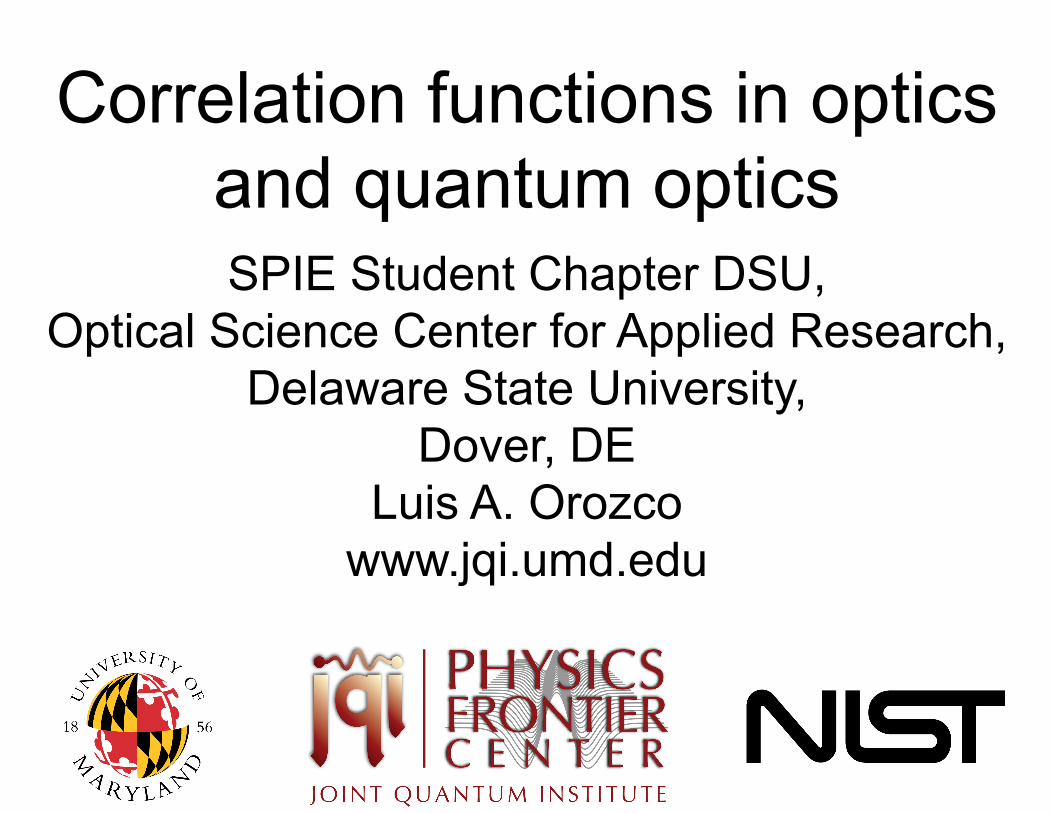
C is the internal product between the output data vector (y) and the value of the expected (fit) function (f(x)) with the input data (x)

C =f (xi )

i∑ yi

f (xi )2

i∑ yi

2

i∑

⎛

⎝⎜

⎞

⎠⎟

1/2 =

!f • !y!f !y

=!F •!Y

Note that there is no reference to error bars or uncertainties in the data points

This correlation coefficient can be between two measurements or a measurement and a prediction… •  C is bounded : -1<C+1 •  C it is cos(φ) where φ is in some abstract

space. •  Correlation does not imply causality!

Think of your data as vectors, it can be very useful.

176

178

180

182

184

186

188

190

192

0 500 1000 1500

Freq

uenc

y sh

ift (a

rb. u

nits

)

distance (tens of microns)

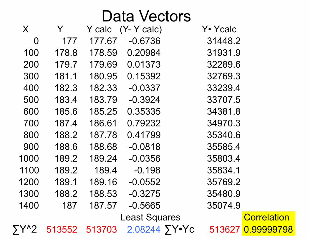
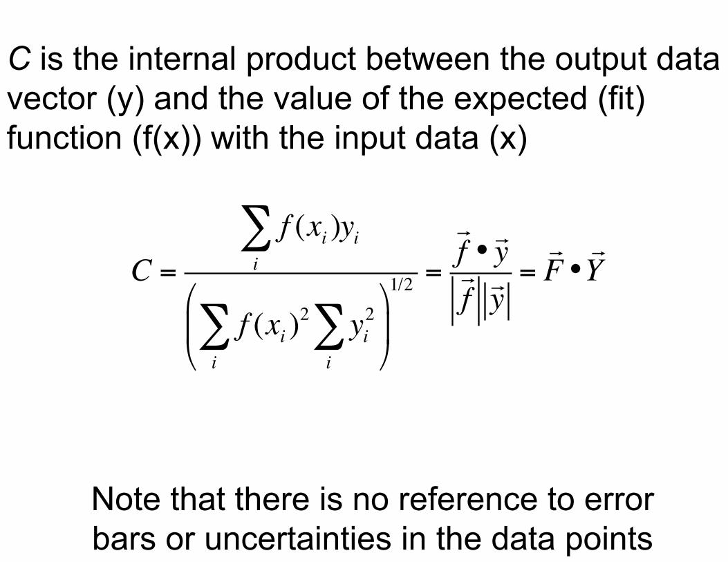
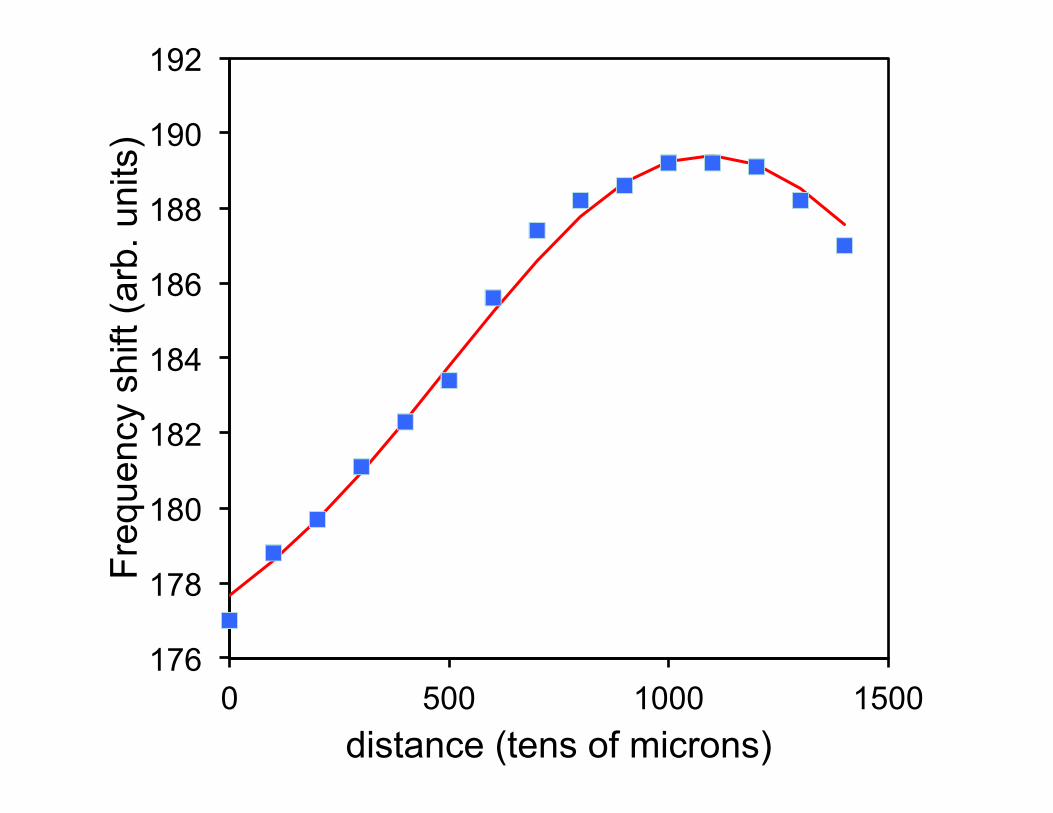
X Y Y calc (Y- Y calc) Y• Ycalc0 177 177.67 -0.6736 31448.2

100 178.8 178.59 0.20984 31931.9200 179.7 179.69 0.01373 32289.6300 181.1 180.95 0.15392 32769.3400 182.3 182.33 -0.0337 33239.4500 183.4 183.79 -0.3924 33707.5600 185.6 185.25 0.35335 34381.8700 187.4 186.61 0.79232 34970.3800 188.2 187.78 0.41799 35340.6900 188.6 188.68 -0.0818 35585.4

1000 189.2 189.24 -0.0356 35803.41100 189.2 189.4 -0.198 35834.11200 189.1 189.16 -0.0552 35769.21300 188.2 188.53 -0.3275 35480.91400 187 187.57 -0.5665 35074.9

Least Squares Correlation∑Y^2 513552 513703 2.08244 ∑Y•Yc 513627 0.99999798

Data Vectors

Correlations are not limited to a single spatial or temporal point.

In continuous functions, such as a time series, the

correlation depends on the difference between the two comparing times.

The correlation can depend on real distance, angular distance or on any other parameter that characterizes

a function or series.

Beyond equal indices (time, position, …)

C(n)=

C(τ)=

Resembles the convolution between two functions

Cross correlation (two functions) Autocorrelation (same function)

The correlation function contains averaging, and you could think of it as some monent over a distribution:

C(τ)=<x(t)x(t+τ)>

Where the probability density has to satisfy the properties of a positivity, integral equal to one…

Now let us think on what happens when the

measurement has signal and noise.

If you only have noise, there are formal problems to find the power spectral density, it is not a simple

Fourier transform.

The Wiener–Khinchin-Kolmogorov theorem says that the power spectral density of noise is the Fourier

transform of its autocorrelation.

Correlation functions in Optics (Wolf 1954)

t

t

Modern coherence theory began in 1954 when Wolf found that the mutual coherence function in free space satisfies the wave equations

The cross spectral density (the Fourier Transform of the correlation) also satisfies the Helmhotz equation:

Then, knowledge of W(0) the cross spectral density (matrix for vector fields) in the source plane allows in principle the calculation of the cross-spectral density function everywhere in the halfspace z>0.

With the associated diffraction integrals

Correlation measurements

The study of optical noisy signals uses correlation functions.

Photocurrent with noise: <F(t) F(t+τ) > <F(t) G(t+τ)>

For optical signals the variables usually are: Field and Intensity, but they can be cross correlations as well.

G(1)(τ) = <E(t)* E(t+τ)> field-field

G(2)(τ) = <I(t) I(t+τ)> intensity-intensity

H(τ) = <I(t) E(t+τ)> intensity-field

How do we measure these functions?

•  Correlation functions tell us something about fluctuations.

•  The correlation functions have classical limits.

•  They are related to conditional measurements. They give the probability of an event given that something has happened.

Mach Zehnder or Michelson Interferometer Field –Field Correlation

)()()(

)(*

)1(

tItEtE

gτ

τ+

=

ττωτπ

ω dgixpeF )()(21)( )1(∫=

Spectrum:

This is the basis of Fourier Spectroscopy

Handbury Brown and Twiss

Can we use intensity fluctuations, noise, to measure the size of a star? Yes. They were radio astronomers and had done it around 1952,

Flux collectors at NarrabriR.Hanbury Brown: The Stellar Interferometer at Narrabri ObservatorySky and Telescope 28, No.2, 64, August 1964

Narrabri intensity interferometerwith its circular railway trackR.Hanbury Brown: BOFFIN. A Personal Story of the Early Daysof Radar, Radio Astronomy and Quantum Optics (1991)

Hanbury Brown and Twiss; Intensity Intensity correlation

2)2(

)(

)()()(

tItItI

gτ

τ+

=

Correlations of the intensity at τ=0

It is proportional to the variance

Intensity correlations (bounds)

The correlation is maximal at equal times (τ=0) and it can not increase.

)()()()(2 22 ττ ++≤+ tItItItICauchy-Schwarz

How do we measure them? Build a “Periodogram”. The photocurrent is proportional to the intensity I(t)

ni

M

i

N

ni

j

i

IItItI

ItIItI

+= =∑∑→+

→+

→

0 0)()(

)()(

τ

τ

•  Discretize the time series. •  Apply the algorithm on the vector. •  Careful with the normalization.

•  The photon is the smallest fluctuation of the intensity of the electromagnetic field, its variance.

•  The photon is the quantum of energy of

the electromagnetic field. With energy ħω at frequency ω.

Quantum optics

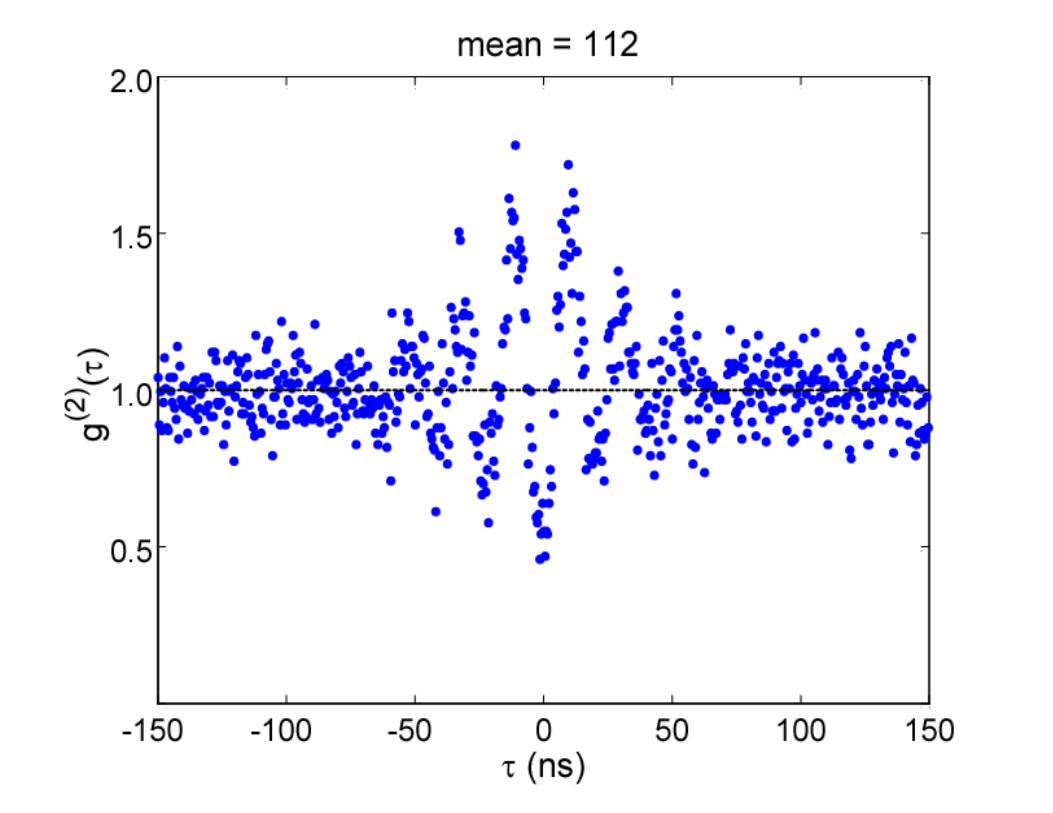
Another form to measure the correlation with with the waiting time distribution of the photons. Store the time separation between two consecutive pulses (start and stop). •  Histogram the separations •  If the fluctuations are few you get after

normalization g(2)(τ). •  Work at low intensities (low counting

rates).

time

Intensity (photons)

An important point about the quantum calculation of g(2)(τ)

The intensity operator I is proportional to the number of photons, but the operators have to be normal (:) and time (T) ordered: All the creation operators do the left and the annihilation operators to the right (just as a photodetector works). The operators act in temporal order.

Quantum Correlations (Glauber):

At equal times (normal order) :

Conmutator : a+a = a a+ −1

a+a+a a = a+(a a+ −1) a = a+a a+a − a+a

a+a+a a = n2 − n where n = a+a

The correlation requires detecting two photons, so if we detect one, we have to take that into

consideration in the accounting.

In terms of the variance of the photon number:

The classical result says:

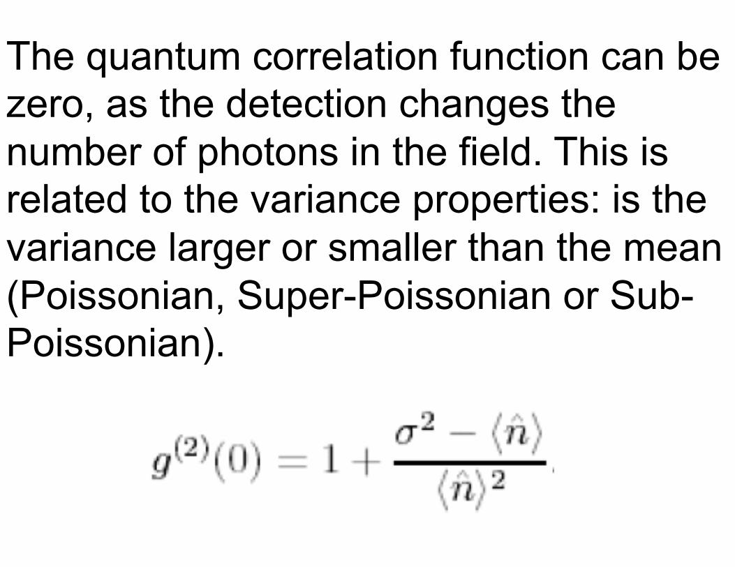
The quantum correlation function can be zero, as the detection changes the number of photons in the field. This is related to the variance properties: is the variance larger or smaller than the mean (Poissonian, Super-Poissonian or Sub-Poissonian).

At equal times the value gives: g(2)(0)=1 Poissonian

g(2)(0)>1 Super-Poissonian g(2)(0)<1 Sub-Poissonian

The slope at equal times:

g(2)(0)>g(2)(0+) Bunched

g(2)(0)<g(2)(0+) Antibunched

Classically we can not have Sub-Poissonian nor Antibunched.

Quantum Correlations (Glauber):

If we detect a photon at time t , g(2)(τ) gives the probability of detecting a second photon after a time τ .

g(2)(τ ) =: I (τ ) :

c

: I :

Correlation functions as conditional measurements in quantum optics.

•  The detection of the first photon gives the initial state that is going to evolve in time.

•  This may sound as Bayesian probabities.

•  g(2)(τ) Hanbury-Brown and Twiss.

Quantum regression theorem

•  The correlation functions can be calculated using the master equation with the appropriate initial and boundary conditions (Lax 1968).

•  This is reminiscent of the propagation of the correlations using the wave equation for the electromagnetic (Wolf 1954, 1955)

Optical Cavity QED

Quantum electrodynamics for pedestrians. No need for renormalization. One or a finite

number of modes from the cavity.

ATOMS + CAVITY MODE

Dipolar coupling between the atom and the mode of the cavity:

El electric field associated with one photon on average in the cavity with volume: Veff is:

!vEdg ⋅

=

effv VE

02εω!

=

SIGNAL

PD

EMPTY CAVITY

LIGHT

C1=g2

κγC=C1N

g≈κ ≈γ

Coupling

Spontaneous emission

Cavity decay Cooperativity for

one atom: C1

Cooperativity for N atoms: C

y

x Excitation

-2Cx 1+x2 Atomic polarization:

Transmission x/y= 1/(1+2C)

Steady State

Jaynes Cummings Dynamics Rabi Oscillations

Exchange of excitation for N atoms:

Ng≈Ω

2g Vacuum Rabi Splitting

Two normal modes

Entangled

Not coupled

0

0.1

0.2

0.3

0.4

0.5

0.6

0.7

0.8

0.9

1

-30 -20 -10 0 10 20 30Frequency [MHz]

Sca

led

Tran

smis

sion

Transmission doublet different from the Fabry Perot resonance

7 663 536 starts 1 838 544 stops

Classically g(2)(0)> g(2)(τ) and also |g(2)(0)-1|> |g(2)(τ)-1|

antibunched

Non-classical

How to correlate fields and intensities?

Detection of the field: Homodyne detection

Source, has to have at least two photons

Conditional Measurement: Only measure when we know there is a photon.

).(ˆ

:)(ˆ)0(ˆ:)(Η τξ

ττ Γ+=

A

BA

The Intensity-Field correlator.

Condition on a Click Measure the correlation function of the Intensity and

the Field:<I(t) E(t+τ)>

Normalized form: hθ(τ) = <E(τ)>c /<E>

From Cauchy Schwartz inequalities:

21)0(0 0 ≤−≤ h

1)0(1)( 00 −≤− hh τ

Photocurrent average with random conditioning

Conditional photocurrent with no atoms in the cavity.

After 1 average

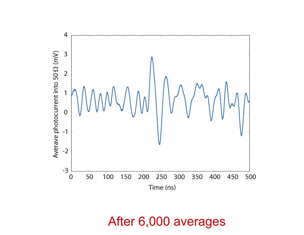
After 6,000 averages

After 10,000 averages

After 30,000 averages

After 65,000 averages

Flip the phase of the Mach-Zehnder by 146o

Monte Carlo simulations for weak excitation:

Atomic beam N=11

This is the conditional evolution of the field of a fraction of a photon [B(t)] from the

correlation function. hθ(τ) = <E(τ)>c /<E>

The conditional field prepared by the click is:

A(t)|0> + B(t)|1> with A(t) ≈ 1 and B(t) << 1

We measure the field of a fraction of a photon!

Fluctuations are very important.

,]1)([)2cos(4)0,( 00

ττπντν dhFS −= ∫∞

!

The fluctuations of the electromagnetic field are measured by the spectrum of squeezing.

Look at the noise spectrum of the photocurrent.

F is the photon flux into the correlator.

Spectrum of Squeezing from the Fourier Transform of h0(t)

Classical g(2) Non-classical h Squeezing

N=13; 1.2n0

Thanks