Quantum nonlinear optics: applications to quantum ...

Louisiana State UniversityLSU Digital Commons

LSU Doctoral Dissertations Graduate School

2009

Quantum nonlinear optics: applications toquantum metrology, imaging, and informationRyan GlasserLouisiana State University and Agricultural and Mechanical College, [email protected]

Follow this and additional works at: https://digitalcommons.lsu.edu/gradschool_dissertations

Part of the Physical Sciences and Mathematics Commons

This Dissertation is brought to you for free and open access by the Graduate School at LSU Digital Commons. It has been accepted for inclusion inLSU Doctoral Dissertations by an authorized graduate school editor of LSU Digital Commons. For more information, please [email protected].

Recommended CitationGlasser, Ryan, "Quantum nonlinear optics: applications to quantum metrology, imaging, and information" (2009). LSU DoctoralDissertations. 850.https://digitalcommons.lsu.edu/gradschool_dissertations/850

QUANTUM NONLINEAR OPTICS:APPLICATIONS TO QUANTUM METROLOGY, IMAGING, AND INFORMATION

A Dissertation

Submitted to the Graduate Faculty of theLouisiana State University and

Agricultural and Mechanical Collegein partial fulfillment of the

requirements for the degree ofDoctor of Philosophy

in

The Department of Physics and Astronomy

byRyan Glasser

B.S. in Physics, University of California Los Angeles, 2005May 2009

Acknowledgments

There are quite a few people who have made this work both possible as well as enjoyable.

Every professor I have worked for and with since my undergraduate career has been an

absolutely wonderful mentor. At UCLA, James Rosenzweig and Gil Travish both showed me

that it was possible to be a good physicist and a fun person simultaneously. This has proved

to help make me a more well-rounded person, which I value tremendously.

I would also like to thank Dr. Phil. I thought my previous bosses would be the only

awesome bosses I would have as a physicist. You certainly proved me wrong.

Then there is my advisor, Jon Dowling. I cannot thank you enough for everything. You

have given me the opportunity to attend countless program reviews and conferences, which

has helped me learn the ropes of being a physicist. Thank you so much for sending me off

to work in a couple of labs, to get my theorist hands dirty. You have been the absolute

best person I can ever imagine working for. I sincerely thank you for all of the experiences

you have given me the opportunity to undertake. I have learned so much from you that no

acknowledgement would ever be sufficient. You are both a great physicist and a sincere, good

person.

I would also like to thank John Howell and his graduate students, Ryan Camacho, Ben

Dixon and Curtis Broadbent. My time spent in your lab in Rochester was an absolute

pleasure. Ben and Ryan, it was wonderful working with both of you while I was there. I

sincerely hope that our career paths may cross again. John, your students think as highly

of you as I do of Dowling, and my short time in your group showed me why. Thank you for

allowing me to work with you and your students, I would happily do it again.

I would also like to thank Jerome Luine, with whom I worked setting up a lab at Northrop

Grumman. I had an absolutely great time working out there with you. I only wish that

I would have been able to stay a little longer so we could have seen some down converted

ii

photons! Thank you for letting me help in the lab. I think STRL is a great idea, and certainly

consists of a wonderful group of people, yourself included.

My friends have certainly helped make this work more enjoyable. All the Barstow kids, I

completely forget about work when I’m with you and have the best of times. Eric, I wish you

would have come out to graduate school at LSU with me. We could have had a repeat of our

fun times from UCLA. Jack, you have shaped my life immensely. I will never forget the good

times we’ve had. I would also like to thank all of my friends from graduate school. Sean, Bill,

and Jeff (big and skinny), as well as many others (you know who you are), have made my

experience in Baton Rouge amazing. We have certainly had some crazy times around ”the

hood.” I came to LSU not knowing anyone, and am leaving knowing so many smart, fun,

solid people. My life over the last four years would have been significantly less fun if you all

were not in it. So, thank you.

I would like to thank my family. All of you have been so incredibly supportive of everything

I have done. Uncle Ron, it’s always great to have a person to talk physics with around the

holidays! Grandma, I cannot imagine having a cooler person for a grandmother.

Finally, I would like to thank my parents, Tom and Sue Glasser. Momo and Dado, you

are the best mother and father a person could ever ask for. You both have hands-down

been the biggest influences in my life. Because of you I strive to be a better person every

day. Your unconditional support in every aspect of my life has made me who I am today. I

cannot possibly thank you enough for everything. I feel blessed to have my parents as my

best friends in the world. I love you both more than anything. This thesis is dedicated to

the both of you.

iii

Table of Contents

ACKNOWLEDGMENTS . . . . . . . . . . . . . . . . . . . . . . . . . . . . . . . . . . . . . . . . . . . . . . . . . ii

ABSTRACT . . . . . . . . . . . . . . . . . . . . . . . . . . . . . . . . . . . . . . . . . . . . . . . . . . . . . . . . . . . . . . vi

1 INTRODUCTION . . . . . . . . . . . . . . . . . . . . . . . . . . . . . . . . . . . . . . . . . . . . . . . . . . . . . 1

1.1 Nonclassical Light and Entanglement . . . . . . . . . . . . . . . . . . . . . . 1

1.2 Metrology, Imaging, and Information . . . . . . . . . . . . . . . . . . . . . . 5

1.2.1 Interferometry and the Shot-Noise Limit . . . . . . . . . . . . . . . . 5

1.2.2 Imaging and the Rayleigh Diffraction Limit . . . . . . . . . . . . . . 7

1.2.3 Information and Cryptography . . . . . . . . . . . . . . . . . . . . . 8

2 QUANTUM STATE REPRESENTATIONS OF LIGHT . . . . . . . . . . . . . . . . 11

2.1 Fock or Number States . . . . . . . . . . . . . . . . . . . . . . . . . . . . . . 11

2.1.1 N00N States . . . . . . . . . . . . . . . . . . . . . . . . . . . . . . . . 13

2.2 Coherent States . . . . . . . . . . . . . . . . . . . . . . . . . . . . . . . . . . 14

2.3 Applications of Quantum States to Interferometry, Imaging and Cryptography 15

2.3.1 Beyond the Shot-Noise and Rayleigh Limits . . . . . . . . . . . . . . 15

2.3.2 Quantum Key Distribution . . . . . . . . . . . . . . . . . . . . . . . . 17

3 OPTICAL NONLINEARITY IN CRYSTALS AND ATOMIC VAPOR . 22

3.1 Second-Order Nonlinear Processes in Nonlinear Crystals . . . . . . . . . . . 22

3.1.1 Spontaneous Parametric Down Conversion . . . . . . . . . . . . . . . 23

3.1.2 Optical Parametric Amplification and Fluorescence . . . . . . . . . . 30

3.2 Nonlinear Processes in Atomic Vapor . . . . . . . . . . . . . . . . . . . . . . 34

3.2.1 Four-Wave Mixing . . . . . . . . . . . . . . . . . . . . . . . . . . . . 34

3.2.2 Coherent Population Trapping and Electromagnetically Induced Trans-parency . . . . . . . . . . . . . . . . . . . . . . . . . . . . . . . . . . 37

4 STIMULATED PARAMETRIC DOWN CONVERSION IN NONLIN-EAR CRYSTALS . . . . . . . . . . . . . . . . . . . . . . . . . . . . . . . . . . . . . . . . . . . . . . . . . . . . . . 41

4.1 Single-Photon Seeded Nonlinear Crystals . . . . . . . . . . . . . . . . . . . . 41

4.2 Coherent State Seeded Nonlinear Crystals . . . . . . . . . . . . . . . . . . . 44

4.3 Entangled-State Seeded Nonlinear Crystals . . . . . . . . . . . . . . . . . . . 47

4.3.1 Post-Selection Applications of the Output State . . . . . . . . . . . . 51

4.3.2 Quantum Key Distribution Scheme Based on Stimulated ParametricDown Conversion . . . . . . . . . . . . . . . . . . . . . . . . . . . . . 54

4.4 N00N State-Seeded Nonlinear Crystals . . . . . . . . . . . . . . . . . . . . . 56

4.5 ChARM and Stimulated Parametric Down Conversion . . . . . . . . . . . . 58

4.5.1 Realistic Experimental Setup and Improvements . . . . . . . . . . . . 65

4.5.2 Calculated Spontaneous Parametric Down Conversion Rates . . . . . 67

iv

5 MULTI-SPATIAL MODE ENTANGLEMENT, ENTANGLED IMAGE TRANS-FER, AND NONLOCAL DOUBLE SLIT INTERFERENCE IN FOUR-WAVE MIXING . . . . . . . . . . . . . . . . . . . . . . . . . . . . . . . . . . . . . . . . . . . . . . . . . . . . . . . 725.1 Joint Quadrature Squeezing Via Four-Wave Mixing . . . . . . . . . . . . . . 735.2 Multi-Spatial-Mode Entanglement in Four-Wave Mixing . . . . . . . . . . . . 755.3 Entangled Image Transfer via Four-Wave Mixing . . . . . . . . . . . . . . . . 775.4 Nonlocal Double Slit Interference Via Two Warm Rubidium Vapor Cells . . 82

6 ALL-OPTICAL ZERO TO PI ONLY PHASE SHIFT . . . . . . . . . . . . . . . . . . 876.1 Coherent Population Trapping Via Optical Pumping in Cesium Vapor . . . . 876.2 Optical Faraday Rotation and the Pi-Only Phase Shift . . . . . . . . . . . . 896.3 Experimental Setup . . . . . . . . . . . . . . . . . . . . . . . . . . . . . . . . 916.4 Results . . . . . . . . . . . . . . . . . . . . . . . . . . . . . . . . . . . . . . . 95

7 CONCLUSIONS . . . . . . . . . . . . . . . . . . . . . . . . . . . . . . . . . . . . . . . . . . . . . . . . . . . . . . . 98

REFERENCES . . . . . . . . . . . . . . . . . . . . . . . . . . . . . . . . . . . . . . . . . . . . . . . . . . . . . . . . . . . 101

VITA . . . . . . . . . . . . . . . . . . . . . . . . . . . . . . . . . . . . . . . . . . . . . . . . . . . . . . . . . . . . . . . . . . . . . 108

v

Abstract

The fields of quantum and nonlinear optics have given rise to a variety of nonclassical states

of light that have been proven to surpass certain limitations set by classical physics. Namely,

certain squeezed and entangled states have been shown to beat the shot-noise limit when

making precision phase measurements in interferometry, as well as write lithographic patterns

that are smaller than classically allowed by the Rayleigh diffraction limit. Additionally, single-

photon sources and entangled photon pairs have given rise to provably secure quantum key

distribution for cryptography.

Producing these quantum states of light has proven a difficult task. Nonlinear crystals,

when pumped by a laser, produce pairs of single photons via the process of spontaneous

parametric down conversion (SPDC). This process is mediated by the second order nonlinear

susceptibility of the material. When pumped in a high gain regime, these crystals give rise

to optical parametric amplification, which is a viable source of squeezed light. The vast

majority of research in this area has focused on crystals that are seeded by vacuum in their

two modes.

This dissertation concerns the field of quantum nonlinear optics. It is an investigation

into the processes that occur when nonlinear materials interact with the electromagnetic

field on the single photon level. I have focused on seeding nonlinear crystals with quantum

states of light, including single photons and entangled states. This process results in various

states directly applicable to interferometry, imaging, and cryptography. Another application

investigated is an absolute radiance measurement via stimulated parametric down conversion

resulting from non-vacuum seeding of a nonlinear crystal.

Additionally, other nonlinear processes, including four-wave mixing, nonlinear magneto-

optical effects and coherent population trapping in warm atomic vapor involving quantum

states of light are investigated. The process of seeding third-order nonlinear interactions,

vi

such as in atomic vapors, gives rise to a variety of interesting, nonclassical phenomena such

as entangled image transfer and nonlocal imaging. Strong analogies between SPDC and four-

wave mixing are drawn. I also experimentally show an all optical pi-only phase shift of one

light beam via another in warm Cesium vapor.

vii

Chapter 1Introduction

1.1 Nonclassical Light and Entanglement

Nonclassical states of light have been studied in depth both experimentally and theoretically

since the emergence of quantum electronics [1]. Much interesting physics has resulted from

this, including the field of quantum optics [2]. Quantum states of light are applicable to

a variety of systems including interferometric, lithographic and cryptographic applications

[4, 5, 6, 7, 8, 9, 10, 11, 12]. In particular, various types of squeezed light are able to surpass

some limitations set by classical physics. Two important examples of this are the ability

to make phase measurements beyond the shot-noise limit, as well as the ability to write

lithographic patterns that are smaller than classically allowed by the Rayleigh limit. Squeezed

light proves to be a promising tool that has many potential real-world applications that go

beyond the classical physics realm [19, 14, 15, 16, 17, 18, 19, 20].

Another extremely important concept in quantum optics is that of entanglement. This

dates back to the Einstein-Podolsky-Rosen paper written in 1935 [21]. The idea is that two

systems, particles for example, become entangled such that if we make a measurement on one

of the systems, we immediately reveal to ourselves the state of the other system regardless

of its distance (spatially or temporally) to us. This ”spooky action at a distance” caused

much concern to EPR, and rightfully so. At first glance, this strange phenomenon appears

to violate causality by passing information between two points faster than the speed of light

(that is, immediately). This is however untrue, as one is unable to communicate or share any

information between the two points without the need of classical communication. Despite

this fact, entanglement retains many ”spooky” and interesting qualities. For example, one

may exploit entanglement to create a provably secure cryptographic key [11]. Additionally,

1

certain entangled states have been shown to also beat the shot-noise limit in interferometry,

as well as the Rayleigh limit in lithography [22, 23, 24, 25].

As one might expect, creating these quantum states of light is not a simple task. The most

commonly used methods available with today’s technology are via nonlinear crystals or alkali

vapor. When discussing single photon type experiments, nonlinear crystals are the backbone

of almost every quantum optics experiment around the globe today. As we will see, the

majority of experiments involving these crystals utilizes an unseeded, low gain limit which

induces a process known as spontaneous parametric down conversion [26, 27, 28, 29, 30, 31].

However, much interesting and new physics arises when we input nonclassical and entangled

light into these crystals, as well as when we look in a higher gain regime [32, 33, 34, 35, 36,

37, 38, 39, 40].

Alkali vapor cells, for example containing Rubidium or Cesium, are also frequently used

to create nonclassical states of light [41, 42, 43, 44, 45, 46, 47, 48]. Many nonlinear effects

may take place when these gases interact with light, such as coherent population trapping,

electromagnetically induced transparency, slow light, and squeezed light production. The

four-wave mixing process in particular has been shown to produce squeezed twin beams, as

well as allow for the creation of entangled images between the output beams.

One of the most intuitive ways to view an electromagnetic field is to look at its phase

space diagram. This is a simple pictorial view of the what we will see are the dimensionless

position and momentum of the state of the electromagnetic field. The phase space diagram

pictorially shows the uncertainty a given state has in the two quadratures depicted. The

uncertainty principle requires that the uncertainty in both quadratures obeys the inequality

〈(∆X1)2〉〈(∆X2)2〉 ≥ 1/16 [2]. A minimum uncertainty state is a state whose uncertainty is

such that the equality holds in the previous sentence’s equation. The vacuum state |0〉 is a

minimum uncertainty state about the center of the phase space diagram, with quadrature

uncertainties 〈(∆X1)2〉 = 〈(∆X2)2〉 = 1/4. It contains equal uncertainty in both quadratures,

and is thus depicted as a filled in circle. The most classical state of light, the coherent state

2

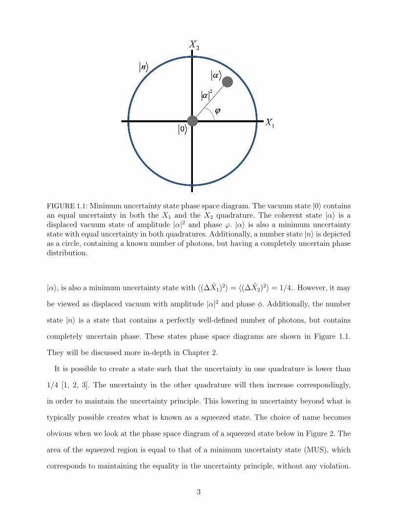
FIGURE 1.1: Minimum uncertainty state phase space diagram. The vacuum state |0〉 containsan equal uncertainty in both the X1 and the X2 quadrature. The coherent state |α〉 is adisplaced vacuum state of amplitude |α|2 and phase ϕ. |α〉 is also a minimum uncertaintystate with equal uncertainty in both quadratures. Additionally, a number state |n〉 is depictedas a circle, containing a known number of photons, but having a completely uncertain phasedistribution.

|α〉, is also a minimum uncertainty state with 〈(∆X1)2〉 = 〈(∆X2)2〉 = 1/4.. However, it may

be viewed as displaced vacuum with amplitude |α|2 and phase φ. Additionally, the number

state |n〉 is a state that contains a perfectly well-defined number of photons, but contains

completely uncertain phase. These states phase space diagrams are shown in Figure 1.1.

They will be discussed more in-depth in Chapter 2.

It is possible to create a state such that the uncertainty in one quadrature is lower than

1/4 [1, 2, 3]. The uncertainty in the other quadrature will then increase correspondingly,

in order to maintain the uncertainty principle. This lowering in uncertainty beyond what is

typically possible creates what is known as a squeezed state. The choice of name becomes

obvious when we look at the phase space diagram of a squeezed state below in Figure 2. The

area of the squeezed region is equal to that of a minimum uncertainty state (MUS), which

corresponds to maintaining the equality in the uncertainty principle, without any violation.

3

FIGURE 1.2: Displaced squeezed vacuum state |ξ〉 in a phase space diagram. Uncertainty inthe X1 quadrature is reduced, thus increasing uncertainty in the X2 quadrature.

These states are very nonclassical, and have many interesting characteristics. We may also

view squeezing between two separate optical beams [1, 2, 3, 47]. Defining the quadrature

operators X1a, X2a for beam ”a” (probe beam) and X1b, X2b for beam ”b” (conjugate), we

can realize the joint quadrature operators:

X1+ = (X1a + X1b)/√

2 and X2− = (Y2a − Y2b)/√

2. (1.1)

When these quadratures are observed to have noise fluctuations below the shot-noise limit

(SNL), they are entangled (or inseparable). When two beams are produced by way of non-

linear, parametric processes, they can exhibit squeezing in joint quadratures, such as photon

number difference between the two modes. Much of the work to produce these twin beams

has been in nonlinear crystals enclosed in resonant cavities [49, 50, 51, 52, 53]. Due to

the presence of the cavity, the output beams are typically macroscopic, yet contain pho-

ton number difference squeezing between the two modes. Another consequence of the re-

strictions set by the resonant cavity are that the output modes are typically single-spatial

mode, thus not allowing for pixel and image entanglement. However, neglecting the cavity,

4

the process involved in these crystal experiments, resulting from the χ(2) nonlinearity, is

parametric down conversion. The interaction Hamiltonian for this process, again neglect-

ing the resonator, is HI = [−εa†b† + ε∗ab], which leads to the unitary evolution operator

S(η) = exp [−ηa†b† + η∗ab] [2]. This is a three wave process, where we have assumed an

undepleted pump such that ε and η are complex numbers rather than operators.

We see that this process produces pairs of photons due to the presence of the operators a

and b. The photon number correlations between these two modes are perfect. Entanglement in

this type of setup is inherently multi-spatial-mode because of the phase-matching conditions

involved. In order to extend this toward a macroscopic beam, these crystals are typically

placed in a resonator in order to increase the effective nonlinearity. However, due to inherent

effects when including the resonant cavity, the multi-spatial-mode entanglement is lost and

one is left with single-spatial-mode twin beams. Due to the Hamiltonian mentioned earlier,

the twin beams will exhibit strong intensity correlations.

As mentioned, entanglement is another key concept in nonlinear and quantum optics.

Strictly speaking, a state is entangled if the state vector describing it is inseparable. For

example, using bra-ket notation such that |1〉a corresponds to one photon in mode a, the

two-mode state (|2〉a|0〉b + |0〉a|2〉b)/√

2 is entangled. Until a measurement is made on one

of the two modes a and b, we must describe the state of the system as having either two

photons in mode a and none in mode b, or vice versa. Entangled states such as this give rise

to improvements beyond those set by classical physics in the fields of interferometry, imaging

and cryptography.

1.2 Metrology, Imaging, and Information

1.2.1 Interferometry and the Shot-Noise Limit

Applications of nonclassical light allow for extremely useful improvements in a variety of

fields. Interferometry, the metrological study of phase, is limited classically by the shot-noise

limit. To understand this, I will take the example of a Mach-Zehnder interferometer, as seen

in Figure 1.3.

5

This is a two-mode device consisting of a beam splitter, two mirrors, a path length dif-

ference between the two arms corresponding to a phase difference, another beam splitter

and detectors. If we input classical light, such as a coherent state (a laser), we obtain the

shot-noise limit which says that the minimum value of the phase difference we measure goes

as ∆φ = 1/√n, where n is the mean number of photons in the input coherent state. This

way of viewing the SNL results from the Poissonian statistics of coherent light, which will be

discussed further in Section 2.1. While it may seem that one can just continue increasing the

number of photons indefinitely, other considerations eventually come into play which limit

the sensitivity, such as radiation pressure.

The other method of seeing how the SNL arises is by viewing it as resulting from vacuum

fluctuations. The example with coherent light results in the SNL when either one or both

of the input ports contains a laser input. However, it has been shown that any time one of

the two input ports is left empty (that is, vacuum input only), the SNL again is the limiting

factor on phase uncertainty [15]. This results in the SNL with any input state, regardless

of how nonclassical it is, so long as one input port remains vacuum. We can now see that

in order to obtain phase information beyond that allowed by the SNL, we must input a

nonclassical state into the interferometer, as well as make sure not to leave either input port

in the vacuum state.

Nonclassical light has a direct application to interferometry in that it can go beyond

the SNL and reach the Heisenberg Limit (HL) ultimate phase sensitivity of ∆φ = 1/N ,

where N is the number of photons input to the interferometer. Squeezed light input into an

interferometer will result not in the HL, but will still be better than the SNL. A variety of

other states have been shown to exhibit phase sensitivity measurements with sensitivities

between the SNL and HL, which is still of much interest due to possible incorporation into

future LIDAR schemes and gravity wave interferometry, such as LIGO [19, 16, 23, 24, 25].

There are however, specific, maximally entangled path states, called N00N states, that do

in fact reach the HL [4, 22, 29, 30]. These are difficult to produce efficiently, though I have

6

theoretically shown a method to create N = 4 N00N states at a relatively high rate which

is discussed in Section 4.3 [36].

FIGURE 1.3: Mach-Zehnder interferometer. This is a two-mode device. However, in thisdiagram one input is left as vacuum. ϕ is a path length difference between the two arms.

1.2.2 Imaging and the Rayleigh Diffraction Limit

One key goal of classical lithography is to write ever smaller diffraction patterns. Clas-

sically, interferometric lithography fringe patterns are limited by the Rayleigh diffraction

limit, which states that laser light of wavelength λ exhibits deposition patterns that scale

as 1 + cos 2φ, where φ = kx and k = 2π/λ. Here φ is the phase shift corresponding to the

path length difference between the two modes of the interferometer and x is the dimension

along the substrate [4]. Thus, the classical method to produce smaller fringes is to decrease

the wavelength of the light being used to write the interference pattern. This suffers from

the limitation that it quickly becomes difficult to work with materials when using very short

wavelengths, such as x-rays.

Nonclassical states have been shown to beat this Rayleigh diffraction limit [29, 30]. For

example, specific states discussed in section 2.2, can write interferometric lithographic pat-

terns that scale as 1 + cos 2Nφ, where N is the total number of photons input into the

interferometer. This allows for writing smaller lithographic patterns at a given wavelength,

7

which will reduce the requirement to move to ever shorter wavelengths to increase fringe

density.

FIGURE 1.4: Interference patterns in imaging. The blue fringes correspond to the Rayleighlimit at a given wavelength. The red fringes then correspond to interference with a quantumstate allowing two times the fringes per cycle.

Another useful application of nonclassical light to imaging is image transfer. Photode-

tectors that are easily available today are much more efficient at visible wavelengths than

say, the far infrared. Due to the correlations produced via nonlinear interactions, images

and information about photon number at one wavelength may transferred to another. These

processes occur in stimulated parametric down conversion as well as stimulated four-wave

mixing [32, 33, 34, 35, 36, 37, 38, 39, 40]. Section 4.5 discusses an experiment that allows

for exactly this kind of photon number information transfer from an infrared source to the

visible region.

1.2.3 Information and Cryptography

Secure transmission of information via cryptographic methods has been around for centuries.

In general, cryptography requires a method of encrypting a message, as well as a method

to decrypt it. The standard scheme involves a party, Alice, encrypting a message via some

algorithm, sending it over an insecure line in which an eavesdropper, Eve, may try to view

the encrypted message, and the receiving party who is to decrypt and recover the original

8

message, Bob. There exists a multitude of cryptography schemes, though many are extremely

easy to break given decent computing power.

Public-key cryptography has become extremely common since the birth of computers. In

this type of cryptography, the encryption method is well known and publicly released such

that many people can encrypt messages. The decryption method is kept secret and only

supposed to be known by the intended receiver of the encrypted message. RSA, which is

a public-key cryptographic algorithm used largely for secure transformation of information

across computers, is not provably (mathematically) secure. The security of the encrypted

message produced via the RSA protocol relies on the mathematical difficulty of factoring a

large number into its constituent primes. Though extremely difficult and needing very large

time frames, factorizing into primes and therefore decrypting a RSA encrypted message is

possible. In fact, in 1994 Shor proved that a quantum computer can factor large numbers

into their prime constituents in polynomial rather than exponential time [55].

On the other hand, a provably (mathematically) secure method of creating and sending

secure messages is the one-time pad. A key used to encrypt a message is used just once, as

well as once to decrypt the message. If the key is truly random, as long as the message to

be encrypted, and only shared between the encrypting and decrypting parties, then the one-

time pad method is completely secure and impossible to be broken. Quantum key distribution

(QKD) schemes, as discussed in section 2.3.3, can reliably create completely random one-time

pads between two parties [6, 7, 8, 11, 56, 57].

Most of the QKD schemes discussed will rely on two parties sharing a random string

of bits. This is called the key and will be used as the one-time pad. The message to be

encrypted is also to be written in binary. The first party encrypts the message by adding the

message and the key base two. They then send the encrypted message to the second party.

This person then decrypts the cryptotext by again adding it to the shared key base two.

The result is the original unencrypted message. This is easily seen by taking the following

9

example. Alice takes her message and adds it to the random key that her and Bob privately

share, resulting in the cryptotext:

message→ 1000110111010

+

key → 0110010101110

cryptotext→ 11100100010100

She then sends the cryptotext to Bob, who then adds it to the privately shared, random key,

base two:

cryptotext→ 1110100010100

+

key → 0110010101110

message→ 1000110111010

Thus, Bob has retrieved the original unencrypted message. Any eavesdropper who may obtain

the cryptotext will see nothing but a random string of bits, due to the fact that the key was

generated randomly to encrypt it.

10

Chapter 2Quantum State Representations of Light

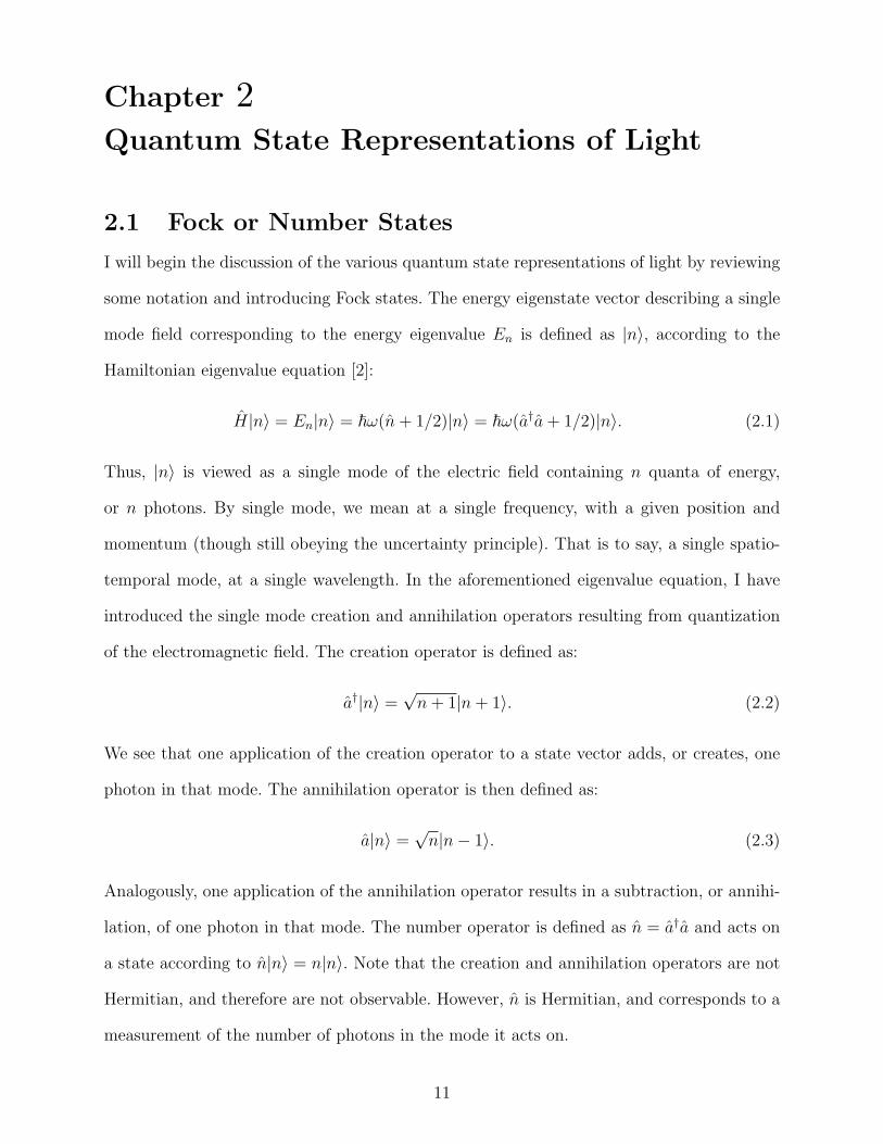
2.1 Fock or Number States

I will begin the discussion of the various quantum state representations of light by reviewing

some notation and introducing Fock states. The energy eigenstate vector describing a single

mode field corresponding to the energy eigenvalue En is defined as |n〉, according to the

Hamiltonian eigenvalue equation [2]:

H|n〉 = En|n〉 = ~ω(n+ 1/2)|n〉 = ~ω(a†a+ 1/2)|n〉. (2.1)

Thus, |n〉 is viewed as a single mode of the electric field containing n quanta of energy,

or n photons. By single mode, we mean at a single frequency, with a given position and

momentum (though still obeying the uncertainty principle). That is to say, a single spatio-

temporal mode, at a single wavelength. In the aforementioned eigenvalue equation, I have

introduced the single mode creation and annihilation operators resulting from quantization

of the electromagnetic field. The creation operator is defined as:

a†|n〉 =√n+ 1|n+ 1〉. (2.2)

We see that one application of the creation operator to a state vector adds, or creates, one

photon in that mode. The annihilation operator is then defined as:

a|n〉 =√n|n− 1〉. (2.3)

Analogously, one application of the annihilation operator results in a subtraction, or annihi-

lation, of one photon in that mode. The number operator is defined as n = a†a and acts on

a state according to n|n〉 = n|n〉. Note that the creation and annihilation operators are not

Hermitian, and therefore are not observable. However, n is Hermitian, and corresponds to a

measurement of the number of photons in the mode it acts on.

11

One can immediately see why this Fock state notation is frequently called number state

notation. These terms will be used interchangeably throughout this dissertation. Note that

the annihilation operator acting on vacuum is zero, a|0〉 = 0, number states are orthogonal,

such that 〈m|n〉 = δmn, and form a complete basis set,∞∑n=0

|n〉〈n| = 1. Additionally, the

creation and annihilation operators obey the bosonic commutation relation such that [a, b†] =

δab. Notationally, I will discuss multimode states which are defined as

|n〉1|m〉2|p〉3 ≡ |n〉|m〉|p〉 ≡ |n,m, p〉. (2.4)

This means there are n photons in mode 1,m photons in mode 2 and p photons in mode 3. The

different modes may be of different frequency or be spatially separated, et cetera. Number

states have a perfectly well-defined number of photons in a given mode, and therefore have

complete phase uncertainty. This can be seen in Figure 1.1. The blue circle is the phase

space diagram for a number state and in reality would be infinitely thin, corresponding to

a well-defined number n, but having a phase distributed from 0 to 2π. This results from

the number-phase uncertainty relation ∆n∆φ ≥ 1, which requires uncertainty in either the

number or phase to increase, as the other decreases.

Quadrature operators associated with the quantized electromagnetic field may now be

defined as [1, 2, 3]:

X1 =1

2(a+ a†) and X2 =

1

2i(a− a†). (2.5)

These may be viewed as dimensionless position and momentum operators, and obey the

uncertainty relation:

〈(∆X1)2〉〈(∆X2)2〉 ≥ 1

16. (2.6)

When the equality in this relationship is met, the state is said to be a minimum uncertainty

state (MUS). If the uncertainty in one quadrature is lower than in the other quadrature,

but the equality is still held, we have a squeezed state. The quadrature whose uncertainty

12

is lower than 1/4, while maintaining a MUS, is the squeezed quadrature. This is evidence of

nonclassical light. It should be noted that the vacuum state |0〉 is a MUS.

2.1.1 N00N States

Using our knowledge of the Fock state basis and entanglement, we are free to introduce

maximally path entangled states known as N00N states. A N00N state is a multimode

entangled state defined as [4]:

|N00N〉 =1√2

(|N, 0〉+ |0, N〉). (2.7)

Thus, N00N states have either N photons in mode 1 and no photons in mode 2, or zero

photons in mode 1 and N photons in mode 2. When discussing these states, the various modes

are differentiated by the fact that they are spatially separated. This is how we arrive at they

description ”maximally path entangled.” In a Mach-Zehnder interferometer, for example,

a N00N state existing between the two beam splitters would correspond to a state where

N photons are in the upper path and none in the lower path, or vice versa. We have no

knowledge of which path the photons are in until we make a measurement on one of the two

modes. A measurement causes the state to collapse and gives us full knowledge of where the

photons are. These states are directly applicable to and show enhancements beyond classical

limits in interferometry and imaging, as discussed in section 2.3.

Creating N00N states with N = 2 is almost a trivial task [58]. This can be done by

inputting one photon into each mode of a beam splitter. This can be easily calculated using

the standard 50:50 beam splitter transformations [2]:

a†1 →1

2(a†3 + ia†4) , a†2 →

1

2(ia†3 + a†4), (2.8)

along with the input |1〉|1〉. The output from the beam splitter will be the N00N state:

|2, 0 : 0, 2〉 ≡ i√2

(|2〉|0〉+ |0〉|2〉). (2.9)

However, creating N00N states with N ≥ 3 is a much more difficult task, with essentially no

efficient schemes existing [59, 60]. I have developed a scheme to create N = 4 N00N states

13

with a large relative efficiency compared to other existing schemes, as will be discussed in

section 4.3 [36].

2.2 Coherent States

A specific kind of minimum uncertainty state containing equal uncertainties in phase and

amplitude (number) is the coherent state. The coherent state may be defined as the state

resulting from an application of the displacement operator on the vacuum, or as the right

eigenstate of the annihilation operator. Using the latter, the coherent state |α〉 is defined as

a|α〉 = α|α〉. Normalized, the coherent state written in a number state basis is [2]:

|α〉 = exp(−1

2|α|2)

∞∑n=0

αn√n!|n〉. (2.10)

The expectation value of the number operator n with regard to a coherent state is

〈α|n|α〉 = |α|2. This means that the average number of photons in the coherent state is

n = |α|2. We can arrive at the shot-noise limit by examining the statistics of the coher-

ent state. Coherent states exhibit Poissonian statistics, which can be seen by taking the

probability amplitude for a measurement and detecting n photons, resulting in

|〈n|α〉|2 = e−|α|2 |α|2n

n!= e−n

nn

n!. (2.11)

Additionally, the photon number uncertainty is ∆n =√n. Thus, we arrive at the very

important equation:

∆n

n=

1√n, (2.12)

which states that the fractional uncertainty in total photon number in a coherent state

decreases as total average photon number increases. Using the number-phase uncertainty

relation of ∆n∆φ ≥ 1, we obtain the shot-noise limit:

∆n =√n ⇒ ∆φ =

1√n, (2.13)

since ∆φ = 1/∆n.

14

Unlike Fock states, coherent states are overcomplete and not orthogonal. This can be seen

by noting that [2]:

|〈β|α〉|2 = e−|β−α|2 6= 0 and

∫|α〉〈α|d2α = π, (2.14)

where |β〉 and |α〉 are two different coherent states. These states are, however, the best

approximation of light emitted from a single-mode laser. That is, only one resonant frequency

inside the resonant cavity containing the lasing material. Coherent states are MUS in which

each quadrature has equal uncertainty, similar to the vacuum state. They have a nonzero

average photon number n as mentioned, thus they can be viewed as displaced vacuum states

(as in Figures 1.1 and 1.2, the vacuum is centered around zero, corresponding to average

photon number of zero). These coherent states are thus the most classical of any quantum

state representations of light and give rise to many classical limitations in interferometry

and imaging.

2.3 Applications of Quantum States to

Interferometry, Imaging and Cryptography

In this section I will discuss more in depth how quantum states of light can be used to

beat classical limitations in interferometry and imaging, as well as discuss quantum key

distribution using number states.

2.3.1 Beyond the Shot-Noise and Rayleigh Limits

As mentioned previously, the shot-noise limit can be viewed as arising from either the Pois-

sonian statistics of coherent (laser) light, or from leaving an input beam splitter port as

vacuum. The latter gives rise to the same fluctuations as coherent light due to vacuum fluc-

tuations. An intuitive way to understand this is by the realization that the vacuum state is a

coherent state of average photon number n = 0, thus containing the same uncertainty. Either

of these scenarios results in a minimum detectable phase of ∆φ = 1/√n in an interferometer.

Though the shot-noise limit has been known for quite some time, the Heisenberg limit of

∆φ = 1/N is the true physical limit for phase estimation. Caves showed in 1981 that the SNL

15

could be surpassed by inputting squeezed light into both input ports of an interferometer

[15]. It has since been shown that a variety of other quantum states can beat the SNL and

approach the HL [19, 16, 23, 24, 25, 22, 29, 30].

N00N states, in particular, achieve exactly the Heisenberg limit. If a N00N state exists in

two arms, and a phase shift is given to one of them, the resulting state is [4]:

1√2

(|N, 0〉+ eiNφ|0, N〉). (2.15)

Before looking at phase estimation, we see that this gives rise to interference patterns, given

an N photon absorbing material at the plane of interference, that scale N times smaller

than would be used with coherent light. One way to see where this N -fold improvement

comes from is by realizing that a coherent state would only pick up a phase shift of eiφ in

the same interferometer. The need for an N photon absorbing material is given by the fact

that we need to measure the number of photons at the interference plane of interest. Taking

the N00N state in equation 2.15, and impinging it on an N-photon absorbing material after

passing through a 50:50 beam splitter results in interference patterns scaling as [4]:

〈N00N | d†N dN

N !|N00N〉 = 1 + cos 2Nφ, (2.16)

where d is the dosing operator, corresponding to the sum of the two modes at the interference

plane. For example, the |ψ〉 = 1√2(|2, 0〉 + e2iφ|0, 2〉) N00N state requires a measurement of

〈ψ|d†2d2|ψ〉, and will achieve interference patterns scaling as 1 + cos 4φ, twice that allowed

by the Rayleigh limit. This is the direct application of quantum states of light to lithography

by beating the classical Rayleigh diffraction limit.

Looking back at phase estimation, one can use either linear error propagation or Fisher

information and show that N00N states achieve the HL of ∆φ = 1/N , where N is the total

number of photons in the N00N state [61]. One way to visualize this phenomena is to examine

the interference pattern of the N00N state in Figure 1.4. The minimum detectable phase can

be viewed as related to the slope of the interference patterns. The N00N state pattern

16

has steeper slopes which in turn leads to a lower minimum detectable phase difference.

This can provide a huge improvement in interferometric systems, such as in LIDAR (light

detection and ranging), if efficient schemes are invented for N00N states of large N . It has

also been shown though that N00N states are susceptible to losses, resulting in decreasing

phase sensitivity [62, 63]. However, more robust number and path-entangled states have been

shown to beat the SNL in the presence of loss [64]. These states contain a nonzero number of

photons in both modes, such that 1√2(|N,M〉+ |M,N〉). A comparison of this state may be

made to a N00N state with number of photons corresponding to the difference between the

two modes, N −M . A simple way of understanding how this state may be more robust to

losses than a N00N state in an interferometer is straightforward. If a photon in a N00N state

is detected anywhere in the interferometer before we make the appropriate measurement,

path information is gained about the entangled state. A detection, or loss, of one photon

in the N00N state case allows for the realization that all N photons were in that mode.

However, in the |N,M : M,N〉 case, a single photon detection will not result in complete

path information, so long as N,M ≥ 1.

It is relatively simple to create an N = 2 N00N state [58]. However, creating larger N

N00N states is more difficult, particularly if one desires a high rate of production. The

entanglement-seeded OPA scheme presented in chapter 4 obtains an N = 4 N00N state

with relatively high probabilities compared to previous schemes [36]. Additionally, a scheme

is shown that allows for creation of the |N,M : M,N〉 states, by utilizing two nonlinear

crystals and non-vacuum seeding.

2.3.2 Quantum Key Distribution

Quantum key distribution was first realized by Bennett and Brassard in 1984 with their

now famous BB84 protocol [56]. There have since been many developments in the field of

QKD, both with respect to the BB84 protocol, as well as the realization of various other

QKD schemes involving different quantum states [6, 7, 8, 11, 57]. The security of all QKD

protocols, while varying somewhat in the specific details, relies on a few axioms of quantum

17

mechanics. Namely, any measurement of a quantum system will disturb it, one cannot mea-

sure a quantum state simultaneously in incompatible bases, and it is impossible to perfectly

clone a quantum state (the ”no-cloning” theorem) [65]. Thus, any attempt by an eavesdrop-

per to gain knowledge of the quantum system used for QKD will alter it and essentially

set off an alarm telling us that an eavesdropper is present. Note that the BB84 protocols

random key generation relies on the incompatible bases concept, specifically non-orthogonal

polarizations.

Quantum key distribution schemes involving entangled states were first realized by Ekert

in 1992 and differed in a couple key areas from the BB84 protocol [57]. While the BB84

scheme’s security (identification of a possible eavesdropper) relied on publicly comparing a

subset of the key, and thus shortening it, the Ekert protocol’s security does not. Additionally,

the BB84 protocol involved one party, Alice, sending single photons which she prepared to the

other party, Bob. Ekert’s protocol involved a central entity sending one part of an entangled

state to Alice and the other to Bob. Of course this central entity can be Alice, who would

just send one mode to Bob and store the other mode where she is. In Ekert’s example he used

the maximally entangled spin singlet state 1√2(| ↑, ↓〉+ | ↓, ↑〉). The central entity would send

the first mode to Alice and the second to Bob. Due to the fact that the state is entangled,

neither Alice nor Bob (or anyone for that matter) knows which state their mode is in until a

measurement is made. However, if measured in the same basis, the entangled state collapses

into either | ↑, ↓〉 or | ↓, ↑〉, with 50% probability.

The protocol goes as follows [57]. Alice has a polarizer with three possible bases for mea-

surement, 0, 45 and 90. Bob has a polarizer with three possible bases for measurement,

two of which are the same as Alice’s, 45, 90 and 135. The central source sends out the

entangled state, one mode to Alice and the other to Bob. Each of them picks, at random, a

basis in which to make their measurement. They then record which spin their particle was in

after the measurement. Alice and Bob then communicate classically over a public line and

tell each other which basis each measurement was made in. Every measurement with which

18

they randomly chose the same basis (1/3 of the time), they will know they have perfectly

anticorrelated measurements of spin, given no eavesdropper. This discussion was made in

order to show that Bell inequality violations may be used to test for eavesdroppers.

An eavesdropper, Eve, may attempt to interfere with the protocol in order to gain infor-

mation about the key. She may place herself between the central source and, say Bob, and

measure his particle before it makes it to him. However, she must also randomly choose a

basis for her measurement. If she picks an incompatible basis relative to Alice’s randomly

chosen basis, her measured spin will be random and not anticorrelated with Alice’s. Eve

would then send another particle to Bob with the spin she measured. Bob then continues the

protocol (without knowing Eve was interfering) and randomly chooses a basis and makes his

measurement. However, if Eve chose an incompatible basis with Alice, even if Bob chose the

same as Alice, Bob’s measured spin will be random rather than anticorrelated with Alice’s.

The security of the system, corresponding to the ability to detect Eve’s presence, relies on

violating a Bell inequality [66]. Alice and Bob publicly compare the results of the measure-

ments in which they did not randomly choose the same basis. They calculate the function

[67]:

S = C[A0 , B45 ]− C[A0 , B135 ] + C[A90 , B45 ] + C[A90 , B135 ], (2.17)

where C[A0 , B45 ] is the correlation coefficient when Alice measures in the 0 basis and

Bob measures in the 45 basis, et cetera. Classically, S ≤ 2. However, quantum mechanics

and the correlations resulting from the entangled state allow for S ≤ 2√

2. Thus, given

perfect experimental conditions neglecting losses, Alice and Bob will achieve S = 2√

2 if

no eavesdropper is present, and less than 2 if Eve was interfering. There exist purification

and error correction schemes to compensate for realistic, lossy systems. Thus, the protocol

is secure and Alice and Bob can detect the presence of an eavesdropper.

Time-energy entangled QKD schemes have also been developed [6, 7]. The primary method

for generating keys via this scheme is via parametric down conversion (SPDC) in nonlinear

19

crystals. This process will be described in-depth in section 3.1.1. The important concept

relating to time-energy QKD is that pairs of photons are created almost simultaneously in

this process, though time between creation of pairs is typically much larger (can be made to

be arbitrarily large by changing experimental parameters such as pump beam power). The

time-energy entanglement existing between the photon pair is discretized, allowing for more

than 10 bits of information per photon [8]. Multiple time-energy QKD schemes have been

recognized, though I will focus on an experiment by Howell [8], since the security of a QKD

scheme resulting from my work is analogous.

The process for generating a key is as follows [8]. Alice creates a pair of time-energy entan-

gled down converted photons, sends one to Bob and keeps one for herself. They then choose,

independently and randomly, to measure their respective photons either directly or after

passing it through a Mach-Zehnder interferometer (in which one arm’s path length is sub-

stantially longer than the other). The reason for Alice and Bob each using a Mach-Zehnder

interferometer is related to the security of the system. Once all measurements are made,

Bob publicly announces to Alice at what time his photons arrived that he sent through

his Mach-Zehnder interferometer. The two interferometers together form a Franson inter-

ferometer [68], and will exhibit fringes when examining coincidence measurements between

the two Mach-Zehnder interferometers. Alice uses Bob’s announced times, along with her

measured interferometer photon arrival times, to create and view the Franson interference

fringes. Visibilities of up to nearly 100% have been demonstrated, corresponding to lack of

an eavesdropper’s presence. Franson interferometers are discussed more in depth in section

3.1.1.

In order to create the one-time pad key, the resulting leftover photons, which did not pass

through either Mach-Zehnder interferometer, are privately time-binned by Alice and Bob

independently. A classical syncronization beam, for example with a period of 64 ns in [8],

is used to determine the initial bin size. They publicly announce to one another which time

bin periods they measured a photon (again a directly measured photon, having not passed

20

through an interferometer). Due to the extremely closely related down converted photon

generation times, they are able to privately time-bin the photons into a subsection of the

initial (64 ns) bin period. These bins have periods on the order of 48 ps experimentally [8],

though theoretically can be smaller. Now that Alice and Bob know in which outer time bin

periods they both measured a photon, they can create a key using an alphabet corresponding

to each of the smaller (ps) time-bins. For simplicity, consider the following example. The outer

time bin is divided into three smaller time bins. Of the smaller time bins, a photon measured

in the first bin will correspond to a 1, in the second will correspond to a 2, and the third a 3.

Due to the fact that Alice and Bob know in which outer time bin they both measure a photon,

as well as the (nearly) simultaneous arrival times of the down converted photons, they can

create a key corresponding to which smaller time bin they measured each photon in. If Alice

and Bob both say they measured a photon in outer time bin one , then if Alice secretly

knows she measured it in smaller time bin two, she knows Bob also measured his photon

in smaller time bin two. This then results in a shared bit of information. By making many

of these measurements, they are able to create a one-time pad. A QKD scheme resulting

from entanglement-seeded optical parametric amplifiers which is similar to this time-energy

entangled QKD scheme is discussed in section 4.3.2.

21

Chapter 3Optical Nonlinearity in Crystals and AtomicVapor

The field of nonlinear optics deals with processes resulting from the interaction of light with

materials whose optical properties change depending on the intensity of the light [1]. The

processes which I will describe are spontaneous parametric down conversion and optical

parametric amplification in nonlinear crystals, as well as coherent population trapping and

four-wave mixing in atomic vapor. In order to understand how these processes occur, we must

describe the dipole moment per unit volume, or polarizability, of a material with regards to

an applied light field. The response in standard optics is linear, such that P (t) = χ(1)E(t).

However, expanding this out in a power series in the field strength such that

P (t) = χ(1)E(t) + χ(2)E2(t) + χ(3)E3(t) + . . . , (3.1)

we may investigate nonlinear optics. Here, χ(2) and χ(3) are the second and third order

nonlinear susceptibilities, respectively. Second-order nonlinear optical processes are three-

wave processes which involve three photons. Only materials that are not centrosymmetric

exhibit a nonzero second-order susceptibility. Third-order nonlinear processes are four-wave

processes involving four photons. These processes are capable of producing nonclassical light,

such as intensity squeezed and entangled light [46, 47].

3.1 Second-Order Nonlinear Processes in Nonlinear

Crystals

Nonlinear crystals are crystals which are not centrosymmetric, and therefore exhibit a

nonzero second-order susceptibility χ(2). Typical crystals used for second-order nonlinear

processes include Beta Barium Borate (BBO), Lithium Iodate (LiIO3), Silver Gallium Sul-

fide (AgGaS2), Silver Gallium Selenide (AgGaSe2) and numerous others. Typical values of

the χ(2) susceptibility are on the order of 10−7 → 10−9 cmstatvolt

[1].

22

FIGURE 3.1: Second order nonlinear processes: second-harmonic generation, sum-frequencygeneration, and difference-frequency generation.

Processes associated with the second order susceptibility involve three waves. The first

discovered experimentally was second harmonic generation, in which two pump photons are

upconverted into a single photon at twice the frequency [69]. This process, for example, is

used frequently to create 532nm lasers. In the ChARM experiment in section 4.5, we were

using a diode pumped solid state laser which produced single mode 532nm laser light. This

device used a Neodymium doped Yttrium Orthovanadate, or vanadate (Nd : Y V O4), diode

laser at 1064nm and frequency doubled it (via second harmonic generation) in a Lithium

TriBorate (LBO) nonlinear crystal.

Subsequent second-order nonlinear processes discovered include sum-frequency generation,

difference-frequency generation, spontaneous parametric down conversion, and special cases

of these including optical parametric amplification and oscillation [1]. These processes are

summed up in Figure 3.1. I will be focusing on spontaneous parametric down conversion in

section 3.1.1, optical parametric amplification in section 3.1.2, and stimulated parametric

down conversion in chapter 4.

3.1.1 Spontaneous Parametric Down Conversion

The process of spontaneous parametric down conversion (SPDC) involves a photon at a

given frequency ωp being down converted into two photons of lower energy ωs and ωi, named

the signal and idler respectively, mediated by the nonzero second-order susceptibility. This

three-wave process conserves energy such that ωp = ωs + ωi. When the two down converted

photons are at the same frequency, such that 2ωp = ωs = ωi, we have degenerate SPDC,

which will be discussed first.

23

The interaction Hamiltonian describing the collinear degenerate SPDC case is [2]:

HI = i~[ei(ωp−2ωs)ta†pa2s − e−i(ωp−2ωs)tapa

†2s ]. (3.2)

Assuming a strong, undepleted pump, which is to say that we are using a strong laser to

pump the crystal and can therefore ignore the loss of pump photons in the crystal due to

down conversion, we may write the pump photons’ operator instead as a complex number

such that ap → ζ. Finally, considering the aforementioned energy conservation requirement,

the time dependency drops out and we are left with the interaction Hamiltonian:

HI = i~[ζ∗a2s − ζa†2s ]. (3.3)

This leads directly to the unitary time-evolution operator for degenerate SPDC:

S(η) = eηa2s−η∗a

†2s , (3.4)

where η = reiφ = ζt is the complex squeezing parameter. Here, the time dependence t is

accounted for in the complex squeezing parameter since it is an interaction time, depending

on the length of the nonlinear crystal involved. This depends on the χ(2) nonlinearity, pump

power, and crystal length. The interaction time is accounted for by this method (essentially

the crystal length, since the interaction time depends on how long the crystal is).

The time-evolution operator transforms the signal (or idler) mode according to the trans-

formations [1, 3]:

a0 → S(η)a0S†(η) = a cosh r + a†eiφ sinh r (3.5)

a†0 → S(η)a†0S†(η) = a† cosh r + ae−iφ sinh r, (3.6)

where I have used the subscript 0 to denote the mode after the transformation (which would

correspond to the transformed mode after the interaction with the crystal and pump beam).

The time-evolution operator acting on the vacuum input signal (or idler) mode creates the

single-mode squeezed vacuum state, expanded out in the Fock state basis [2]:

S(η)|0〉 =1√

cosh r

∞∑n=0

[(2n)!]12

2nn!einφ tanh rn|2n〉. (3.7)

24

We can immediately see that only even numbers of photons exist in the output signal (or

idler) mode. This results directly from the a†2 term in the evolution operator. This single-

mode squeezed vacuum is essentially a generalization of the two-mode squeezed vacuum,

discussed next. By controlling the crystal cut, the phase-matching conditions are altered

such that when pumped in one direction, the crystal will down convert photons (the a†

terms), while when pumped at half the frequency in the opposite direction, it will result

in up conversion (the a terms). Since we are focusing on down conversion throughout this

dissertation, we will be concerned with the a† terms.

In general, down converted pump photons may produce signal and idler photons of different

frequencies, in different spatial modes (non-collinear). The interaction Hamiltonian for the

nondegenerate SPDC case is [2]:

HI = i~[ei(ωp−ωs−ωi)ta†pasai − e−i(ωp−ωs−ωi)tapa†sa†i ]. (3.8)

Again taking the undepleted pump approximation, as well as conserving energy, we obtain

the simplified interaction Hamiltonian:

HI = i~[ζ∗asai − ζa†sa†i ]. (3.9)

We then obtain the evolution operator for non degenerate SPDC,

S(ξ) = eξ∗asai−ξa†sa†i , (3.10)

where ξ = reiφ is the two-mode squeezing parameter. I will now relabel the mode operators

such that a corresponds to the signal mode, and b corresponds to the idler mode, for visual

simplicity. Similar to the single-mode squeezing evolution operator, the two-mode squeezing

evolution operator transforms the input signal and idler modes according to [2, 3, 36]:

a0 → S(ξ)a0S†(ξ) = a cosh r + b†eiφ sinh r (3.11)

a†0 → S†(ξ)a†0S(ξ) = a† cosh r − be−iφ sinh r (3.12)

b0 → S(ξ)b0S†(ξ) = b cosh r + a†eiφ sinh r (3.13)

b†0 → S†(ξ)b†0S(ξ) = b† cosh r − ae−iφ sinh r (3.14)

25

Here I have again relabeled the mode operators with the subscript 0, in order to differentiate

the input from the output, or transformed, mode operators.

Application of the two-mode squeezing operator to the two-mode squeezed vacuum results

in the two-mode squeezed vacuum state [2]:

S(ξ)|0, 0〉 =1

cosh r

∞∑n=0

(−eiφ)n tanhn r|n, n〉. (3.15)

We immediately see that the number of photons is the same in each of the two output modes.

In fact, the variance of the number difference between the two modes is easily shown to be:

∆(na − nb) =√

(∆na)2 + (∆nb)2 − 2(〈nanb〉 − 〈na〉〈nb〉) = 0. (3.16)

This is the origin of the number correlations between photons in the two modes. If we measure

one photon in the signal mode, we know that exactly one photon exists in the idler mode.

Similarly, if we measure n photons in the signal mode, we know there are exactly n in the

idler.

The spontaneous parametric down conversion regime corresponds to when the gain r is

sufficiently small such that we can neglect all terms in the two-mode squeezed vacuum except

for |0, 0〉 and |1, 1〉. This is easily achievable experimentally due to the fact that the second

order susceptibility is so small. There are two types of SPDC, Type I and Type II. Type

I SPDC corresponds to the case when the two created photons have parallel polarizations,

whereas Type II SPDC produces signal and idler photons that are orthogonally polarized

to one another. Energy conservation, along with the phase-matching condition ~kp = ~ks + ~ki,

determines which type of SPDC will occur given a specific crystal cut.

Due to the fact that many photon pairs, each at different frequencies, can satisfy the

phase-matching and energy conservation conditions, the output modes of a SPDC crystal

contain a spectrum of photons. Experimentally, typical pump beams are gaussian, which

results in uncertainties with regards to the position and momentum correlations between the

down converted photons. This will result in the SPDC state containing information about

26

FIGURE 3.2: Schematic of Type I SPDC. The pump beam is incident on a nonlinear crystal.The output contains a spectrum of pairs of down converted photons that each satisfy thephase-matching conditions. Pinholes are typically used to select out specific down convertedpairs such that the photon number correlations may be taken advantage of.

the pump and input beam profiles and will be discussed in Chapter 5 when making analogies

between four-wave mixing and parametric down conversion [37, 38, 46]. I will be assuming

an infinite plane wave pump, as well as a thin crystal, in order to simplify the output states

and view more directly the various degrees of entanglement exhibited between the down

converted photons. Now, again due to the fact that many pairs of photons are produced at

different frequencies, I will typically be assuming that pinholes and interference filters are

used in order to pick out two specific modes. This is how we arrive at the biphoton state

|1, 1〉, with one photon in each of the two specific states we are interested in. A diagram of

Type I SPDC, without pinholes or filters, is shown in Figure 3.2.

Assuming a monochromatic pump perpendicular to the face of the nonlinear crystal, as

well as the paraxial approximation, the output SPDC state can be written [37, 38]:

|SPDC〉 = |0〉s|0〉i + κ

∫d~ki

∫d~ksWp(~ki + ~ks)|1〉s|1〉i. (3.17)

Here κ is a constant, ~ks and ~ki are the wave vectors of the signal and idler respectively, and

Wp is the pump’s angular spectrum. This equation has immediate consequences which allow

for transfer of images between all of the modes involved in the SPDC process. This will be

further discussed in chapters 4 and 5. However, now I will be discussing the simplified output

state of SPDC, in which I consider filtering out only two correlated modes from the entire

27

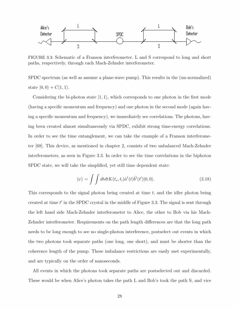
FIGURE 3.3: Schematic of a Franson interferometer. L and S correspond to long and shortpaths, respectively, through each Mach-Zehnder interferometer.

SPDC spectrum (as well as assume a plane-wave pump). This results in the (un-normalized)

state |0, 0〉+ C|1, 1〉.

Considering the bi-photon state |1, 1〉, which corresponds to one photon in the first mode

(having a specific momentum and frequency) and one photon in the second mode (again hav-

ing a specific momentum and frequency), we immediately see correlations. The photons, hav-

ing been created almost simultaneously via SPDC, exhibit strong time-energy correlations.

In order to see the time entanglement, we can take the example of a Franson interferome-

ter [68]. This device, as mentioned in chapter 2, consists of two unbalanced Mach-Zehnder

interferometers, as seen in Figure 3.3. In order to see the time correlations in the biphoton

SPDC state, we will take the simplified, yet still time dependent state:

|ψ〉 =

∫ ∫dtdtK(ts, ti)a

†(t)b†(t′)|0, 0〉. (3.18)

This corresponds to the signal photon being created at time t, and the idler photon being

created at time t′ in the SPDC crystal in the middle of Figure 3.3. The signal is sent through

the left hand side Mach-Zehnder interferometer to Alice, the other to Bob via his Mach-

Zehnder interferometer. Requirements on the path length differences are that the long path

needs to be long enough to see no single-photon interference, postselect out events in which

the two photons took separate paths (one long, one short), and must be shorter than the

coherence length of the pump. These imbalance restrictions are easily met experimentally,

and are typically on the order of nanoseconds.

All events in which the photons took separate paths are postselected out and discarded.

These would be when Alice’s photon takes the path L and Bob’s took the path S, and vice

28

versa. Only the events where the signal and idler both took either the short or long path are

saved. By using the time-dependent state in the previous paragraph, along with standard

beam splitter operators, one can show that interference will occur between the short and

long paths of the interferometers when looking at coincidence time measurements between

Alice and Bob’s detection events. The two-photon rate of detection is then [70]:

R = 1 + cosφe−δτ2∆2

, (3.19)

where δτ is the path length difference between Alice and Bob’s interferometers (each of the

arms), and ∆ is the spectral bandwidth of the filters used to pick out the biphoton state

from the SPDC process. This equation shows that there will be interference in an envelope.

When the path length differences between each path of the two interferometers is zero, 100%

fringe visibility is obtained. This interference is a fourth-order interference, which clearly

shows there exists time correlations between the two photons created via SPDC.

A similar kind of correlation is also present in the biphoton state |1, 1〉. Due to the phase-

matching condition, the directions of the photons produced are well-defined and correlated.

Note there will be some uncertainty in each photons direction of propagation due to spatial

considerations of the pump, finite size of the pinholes used to select the biphotons, finite

bandwidth of the filters used for the same purpose, among other experimental non-idealities.

However, once the state is post-selected into the biphoton state, the correlations in spatial

modes (that is to say, direction) are still strong. A variety of experiments have shown inter-

ference patterns with respect to this kind of correlation with visibilities higher than allowed

classically. For most of the discussions in this dissertation, it suffices to take the output state

in perfectly well-defined modes, neglecting experimental imperfections.

I mentioned previously that creating an N = 2 N00N state is a relatively simple process

[2, 58]. To see how this is done, we consider the biphoton output of a Type I SPDC crystal.

Neglecting the vacuum contribution, since it will contribute nothing to photon counting

measurements at the output, we will take the SPDC output state |ψ〉 = |1, 1〉. This two-

29

mode state input to a 50 : 50 beam splitter will result in:

1√2

(|2, 0〉+ |0, 2〉), (3.20)

with 100% probability. This does not generalize to higher order outputs, which is part of the

problem when trying to efficiently create larger number N00N states.

Until now, I have been focusing on Type I SPDC. Type II SPDC offers the possibility of

post-selecting out states that are polarization entangled [71, 72, 73]. In Type II SPDC, down

converted photons emerge in two cones, one with extraordinary polarization and the other

ordinary. By placing pinholes and/or interference filters at the two points where the cones

intersect, we are selecting out the state:

1√2

(|H,V 〉+ |V,H〉), (3.21)

where |H,V 〉 corresponds to one horizontally polarized photon in the first mode, and one

vertically polarized photon in the second mode. This is due to the fact that since we are

looking at the point where the cones overlap, we are unable to say which of the two points

contains a horizontally polarized photon, and which contains a vertically polarized photon.

This type of entanglement will not be discussed much further, nor Type II SPDC in general.

We now see that the process of spontaneous parametric down conversion produces biphoton

states that exhibit various kinds of entanglement and numerous correlations. The focus of

much of the rest of this dissertation will utilize the spatial, temporal, and energy correlations

discussed in this section. The major concept behind this is the idea that ”by measuring one

mode, I obtain specific information about the state of the other mode,” with regards to

number of photons in particular. This time-energy entanglement has many applications,

such as to QKD, and can be used in various non-vacuum input to nonlinear crystals schemes

which I will discuss in chapter 4 [32, 33, 34, 35, 36, 37, 38, 39, 40].

3.1.2 Optical Parametric Amplification and Fluorescence

The processes of optical parametric amplification and fluorescence (or generation) are other

χ(2) processes, and are intimately related to spontaneous parametric down conversion [5, 9,

30

10, 12, 19, 14, 15, 16, 17, 19, 20, 28, 35]. Essentially, optical parametric fluorescence is a

nonlinear crystal operating in the high gain regime, as opposed to the low gain regime in

which SPDC dominates and any terms higher than |1, 1〉 may be neglected. The interaction

is the same as that which takes place in SPDC, namely [2, 36]:

a0 → S(ξ)a0S†(ξ) = a cosh r + b†eiφ sinh r (3.22)

a†0 → S(ξ)a†0S†(ξ) = a† cosh r + be−iφ sinh r (3.23)

b0 → S(ξ)b0S†(ξ) = b cosh r + a†eiφ sinh r (3.24)

b†0 → S(ξ)b†0S†(ξ) = b† cosh r + ae−iφ sinh r. (3.25)

Unlike the SPDC case, the high gain requires that we do not neglect the higher order terms

in the output state. The output, again in the Fock basis, will be:

S(ξ)|0, 0〉 =1

cosh r

∞∑n=0

(−eiφ)n tanhn r|n, n〉. (3.26)

Now, the gain of the OPA, r, depends on the pump amplitude, length of the nonlinear crystal,

and effective nonlinearity of the crystal. This is the case when the initial signal and idler

modes are vacuum. Thus, this can be viewed as an amplification of vacuum fluctuations;

hence the term fluorescence or generation.

When one of the signal or idler modes is seeded with a state other than vacuum (that is to

say, an input light field at the frequency of the signal for example), the state will be amplified

due to energy transfer from the pump. This is the case of optical parametric amplification [9].

We have seen that pump photons down convert into photonic modes that satisfy the phase-

matching and energy conservation conditions. However, polarization also plays an important

role, and will lead to a discussion on phase-sensitive and phase-insensitive amplifiers. Let us

take the example of a crystal cut for a degenerate Type II parametric interaction, such that

the signal and idler modes are perpendicularly polarized with respect to one another, but are

the same frequency. If we pump the optical parametric amplifier (OPA) with a beam that is

polarized parallel with respect to the signal (and therefore perpendicular to the idler), only

31

the signal mode will be excited. As we shall see, this will result in a phase-insensitive amplifier.

However, if the pump is polarized at 45 with respect to both the signal and idler modes,

both modes will be excited and will result in a phase-sensitive amplifier. These two processes

produce fundamentally different outputs, namely that the phase-sensitive amplification case

can result in a lower than classically allowed noise floor. Note that in future chapters I will

use the term OPA when discussing a high-gain system regardless of what is seeding the signal

and idler modes. SPDC will be used to denote the specific scenario when we neglect all but

the vacuum and biphoton outputs of a pumped nonlinear crystal.

Since we are now dealing with a large number of photons in the signal and/or idler (de-

pending on the polarization of the pump and which crystal cut is involved), we can evaluate

the number of photons in, for example, the signal mode a, which is:

na = a†a = a†a cosh2 r + bb† sinh2 r + (a†b†eiφ + abe−iφ) cosh r sinh r. (3.27)

This corresponds to an intensity measurement of mode a [9].

Looking first at the case in which the pump and signal are polarized parallel to one another,

the output signal intensity is [9]:

a†a = a†a cosh2 r + sinh2 r = na cosh2 r + sinh2 r, (3.28)

due to the fact that the idler mode is not excited. Alternatively, the fact that the idler mode

is initially vacuum necessarily makes the terms 〈n, 0|a†b†|n, 0〉 and 〈n, 0|ab|n, 0〉 go to zero

and sinh2 r〈n, 0|bb†|n, 0〉 = sinh2 r, since 〈n|m〉 = δm,n for both modes. Even for weak input

signals, n 1, so we may neglect the sinh2 r term, which shows we obtain an amplification

of the input signal by a gain factor of g = cosh2 r. There is no phase information about the

pump or signal and idler modes, and thus no dependence of the amplification on the relative

phase. It is then straightforward to show that we will obtain a noise figure, defined as [9]:

N =(signal − to− noise)in(signal − to− noise)out

(3.29)

32

of N = 2− 1/g, which in the high gain (g) limit approaches a decrease in the signal-to-noise

ratio by a factor of two. As a matter of fact, this result holds for any sort of phase-insensitive

amplifier, including strictly classical amplifiers.

A phase-sensitive amplifier may be realized by taking the previous example, but pumping

with a beam that is polarized at 45 with respect to both the signal and idler, rather than

perpendicular to one of the two. In this case, both the signal and idler modes are excited,

resulting in a different scenario. Making use of the identities 2 sinh r cosh r = sinh 2r and

cosh2 r+sinh2 r = cosh 2r, along with the approximation that n 1, we arrive at an output

intensity of [9]:

〈N〉 = n cosh 2r + n sinh 2r cosφ. (3.30)

This depends on the phase φ, which is the relative phase difference between the pump, and

the signal and idler modes together. Hence, we have phase-sensitive amplification. Looking at

the φ = 0 quadrature, we see an amplification of g = e2r, while in the other φ = π quadrature

we see a deamlification of g =−2r. In this particular case under the assumption of n 1,

the noise figure goes to one, corresponding to noiseless amplification. However, in reality,

we are neglecting the sinh2 r term, which is amplification of the vacuum. This is because we

are looking at high gain values and thus not looking at only the quantum case of SPDC, in

which vacuum fluctuations and creation of single photons must be accounted for. This noise

will become important in chapter 4 when I discuss quantum seeding of optical parametric

amplifiers, particularly when examining the low gain regime. This is, however, in a sense the

most noiseless amplification possible. In addition, the photon number correlations existing

between the two output modes will prove to be useful, even when accounting for vacuum

amplification.

It is easy to see that SPDC, as discussed in the previous section, is a low gain limit of an

OPA. Taking the general output state from an OPA, namely:

S(ξ)|0, 0〉 =1

cosh r

∞∑n=0

(−eiφ)n tanhn r|n, n〉, (3.31)

33

the n = 0 term corresponds to vacuum and the n = 1 term corresponds to the biphoton

SPDC output state. In the previous section, I showed that inputting the SPDC output state

into a balanced beam splitter produced the N = 2 N00N state. However, if we input the

more general OPA output state into a 50 : 50 beam splitter, we will obtain the state:

|ψ〉 =∞∑n=0

n∑m=0

Cmn|2n− 2m〉|2m〉. (3.32)

For n = 1, we obtain the N = 2 N00N state. However, every n ≥ 2 output state will contain

N00N state terms, as well as intermediate states with less photons in each mode than the

N. This provides another difficulty in obtaining N00N states larger than N = 2.

3.2 Nonlinear Processes in Atomic Vapor

Interactions between lasers and atomic vapor give rise to numerous interesting physical

phenomena [1]. Typically alkali atoms are used, such as Rubidium (Rb) or Cesium (Cs), due

to their one outer shell electron. Most of these interactions consist of probing the atomic

transitions of the fine structure sublevels with beams at the appropriate frequencies. Dipole

allowed and unallowed transitions between the sublevels allow for various system structures,

such as lambda, vee and double lambda schemes. I will discuss two processes which relate

to my research, namely four-wave mixing which is a χ(3) process and coherent population

trapping, which is the physical basis for a variety of effects, including electromagnetically

induced transparency [1, 41, 42, 43, 44, 45, 46, 47, 74, 75, 76, 77, 78].

3.2.1 Four-Wave Mixing

In the previous section, I discussed second-order nonlinear processes involving the χ(2) suscep-

tibility. The next highest order nonlinear susceptibility is χ(3), which mediates four-photon

interactions. The most general of these interactions is four-wave mixing (4WM) involving

four distinct modes of different frequency, spatial direction and various polarizations. Due

to the fact that the third-order susceptibility is a fourth-order tensor containing 81 terms,

a large number of interaction possibilities exist [1]. Two examples of these are depicted in

34

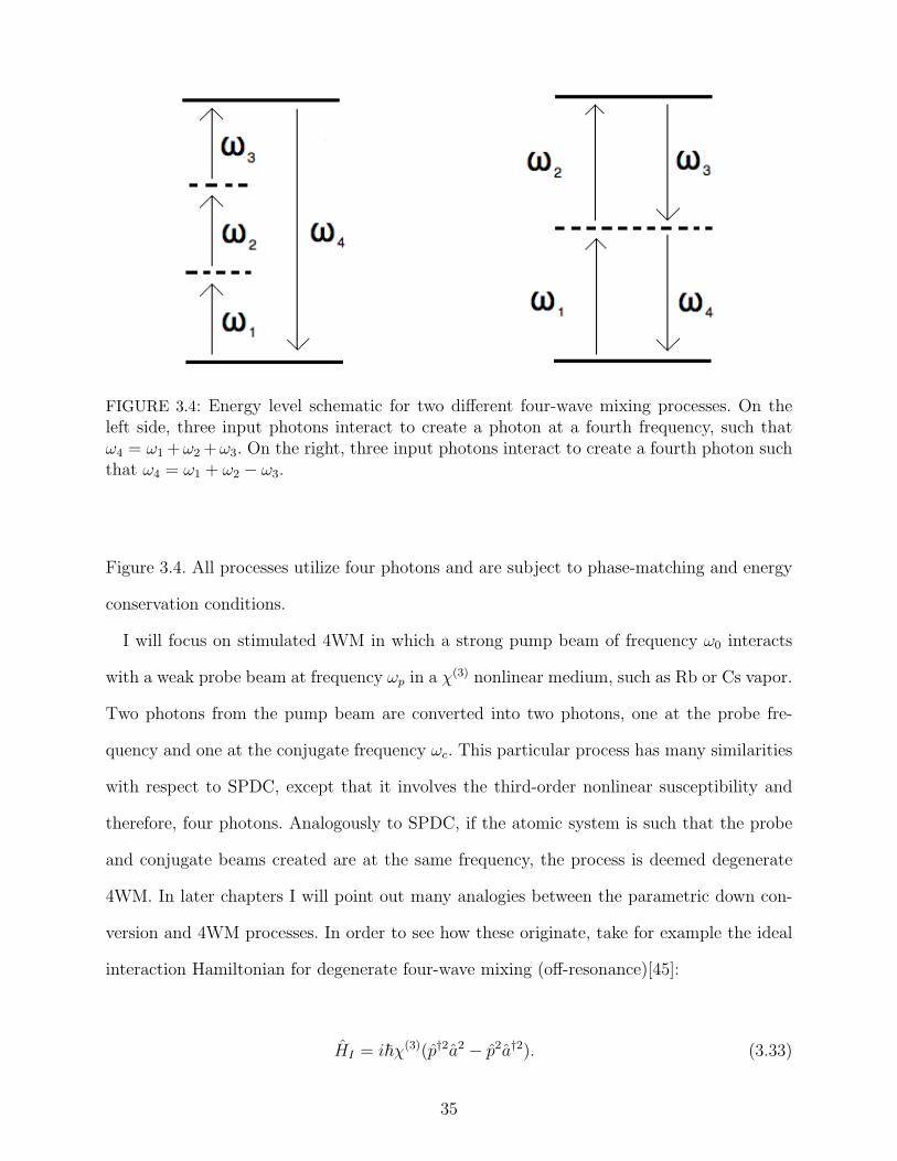
FIGURE 3.4: Energy level schematic for two different four-wave mixing processes. On theleft side, three input photons interact to create a photon at a fourth frequency, such thatω4 = ω1 +ω2 +ω3. On the right, three input photons interact to create a fourth photon suchthat ω4 = ω1 + ω2 − ω3.

Figure 3.4. All processes utilize four photons and are subject to phase-matching and energy

conservation conditions.

I will focus on stimulated 4WM in which a strong pump beam of frequency ω0 interacts

with a weak probe beam at frequency ωp in a χ(3) nonlinear medium, such as Rb or Cs vapor.

Two photons from the pump beam are converted into two photons, one at the probe fre-

quency and one at the conjugate frequency ωc. This particular process has many similarities

with respect to SPDC, except that it involves the third-order nonlinear susceptibility and

therefore, four photons. Analogously to SPDC, if the atomic system is such that the probe

and conjugate beams created are at the same frequency, the process is deemed degenerate

4WM. In later chapters I will point out many analogies between the parametric down con-

version and 4WM processes. In order to see how these originate, take for example the ideal

interaction Hamiltonian for degenerate four-wave mixing (off-resonance)[45]:

HI = i~χ(3)(p†2a2 − p2a†2). (3.33)

35

Making the undepleted pump approximation again, we replace the pump beam mode’s op-

erator p with a complex number and obtain the interaction Hamiltonian:

HI = i~(ζ∗a2 − ζa†2). (3.34)

We immediately see that this is exactly equation 3.3 for degenerate collinear SPDC, with

the exception that ζ contains χ(3) in place of the χ(2) term. Similar extensions may be made

to nondegenerate 4WM and nondegenerate SPDC. These quantum mechanical similarities

give rise to the analogies that will be drawn between these two processes.

FIGURE 3.5: Schematic of a double-lambda type scheme. This will give rise to nondegeneratefour-wave mixing, with photon number correlations existing between the output probe andconjugate beams. The pump beam is at frequency ω0, the probe is at frequency ωp and theconjugate beam is at frequency ωc.

I will be considering the more general nondegenerate stimulated 4WM in which ωp 6=

ωc. As mentioned, two pump photons interact with the medium to create two photons in

other modes, one probe (ωp) and one conjugate (ωc). This process draws many analogies to

stimulated parametric down conversion. First, the probe and conjugate (named this since

its field is the conjugate of the probe) are analogous to the signal and idler modes in PDC.

Secondly, the probe and conjugate beams are subject to energy conservation and phase-

matching conditions relative to the pump beam, just as in PDC. Thirdly, in chapter 5 I will

be describing a scheme which involves seeding the 4WM process with a probe beam, while

leaving the input conjugate mode as vacuum, similar to previously described non-vacuum

36

seeding of nonlinear crystal processes. Lastly, strong photon number correlations arise from

the 4WM process, just as between the signal and idler output modes of PDC [47].

Due to the fact that one four-wave mixing event produces exactly one probe and one con-

jugate photon, analogous to one down conversion event (though involving two pump photons

rather than one), strong correlations arise between the output modes. Many experiments uti-

lize 4WM in optical fibers in order to produce photon pairs, rather than nonlinear crystals.

However, in a more macroscopic sense, intensity difference squeezing has been shown between

the output probe and conjugate beams produced via 4WM in atomic vapor [47, 46]. It should

be noted that the output beams are narrowband due to the fact that the 4WM process relies

on the photons having frequencies very near atomic resonances. This is one difference from

the SPDC process, in which the output contains a large spectrum of down converted photon

pairs. Regardless, when looking at the joint quadratures between the probe and conjugate

beams, corresponding to the intensity difference between the two modes, squeezing of up to

8dB below the shot-noise limit has been experimentally demonstrated [48].

More recently, the spatial-mode properties of the resulting probe and conjugate beams have

been investigated. Due to the photon number correlations between the probe and conjugate

photons produced in the 4WM process, various spatial modes contain photon pairs similar

to the output spatial modes of parametric down conversion [47, 48, 46]. Armed with the

information about 4WM discussed in this chapter, I will describe in more depth the resulting

correlations and their applications, as well as discuss the multi-spatial mode entanglement

produced via 4WM in chapter 5 [47, 46].

3.2.2 Coherent Population Trapping and ElectromagneticallyInduced Transparency

An important process involving optical beams and atomic vapors that needs to be explained

to understand the experiment I performed at the University of Rochester (discussed in chap-

ter 6) is coherent population trapping [79, 80, 81, 82]. The general idea behind this is that

atoms in the vapor can be coherently prepared by a coherent beam (laser) into quantum

37

states such that interference between certain state amplitudes can result in modification of

the atomic response to the beam [2, 44, 82]. An exemplary process resulting from this is

electromagnetically induced transparency (EIT) [44, 82]. In EIT, atoms that are normally

absorbing to light of a certain frequency become transparent to it, due to the presence of an

optical beam.

The physical process behind such phenomena as EIT is coherent population trapping

(CPT) [44]. In CPT, the electrons in an atomic ensemble are, in a sense, forced into specific

energy levels from which they are unable to escape. Optical pumping, the process of pump-

ing an atomic vapor with circularly polarized light in order to induce coherent population

trapping due to hyperfine selection rules, will be discussed in chapter 6 [78]. EIT is a simple

example utilizing CPT, involving a three-level lambda-type system, as shown in Figure 3.6.

FIGURE 3.6: Lambda scheme for EIT. The strong control beam is at frequency ωc and theprobe is at ωp. δ13 and δ23 are the probe and control detunings from the state |3〉, respectively.

Qualitatively, the presence of only one of either the control or probe beam will result in

absorption and reemission, resulting in the system being opaque to either beam. However,

if both beams are present and the two detunings sum up to the difference between states

|1〉 and |2〉, quantum interference of the states’ probability amplitudes results in a dark

state [44, 82, 79]. That is, state |3〉 is no longer reachable and the system is in a coherent

superposition of states |1〉 and |2〉 only. Thus, the beams will no longer be absorbed and the

38

material is now transparent at these frequencies. This is an example of coherent population

trapping because we can see that the electrons are ”trapped” in states |1〉 and |2〉.

In order to see how this works more in depth, we will look at the interaction Hamiltonian

for a 3-level atomic system interacting with a beam at frequency ωp and ωc as depicted in

Figure 3.6. The frequency for the |2〉 → |3〉 transition is ω2 and the frequency for the |1〉 → |3〉

transition is ω1. The detunings from these transitions will be defined as δ13 = ω1 − ωp and

δ23 = ω2 − ωc. The interaction Hamiltonian for the three level system interacting with the

two beams is then [82]:

HI =−~2

0 0 Ωp

0 −2(δ13 − δ23) Ωc

Ωp Ωc −2δ13

(3.35)

where Ωp and Ωc are the Rabi frequencies resulting from the probe and control beams,

respectively. When the detunings are equal, such that δ13 = δ23 ≡ δ, the eigenvalues of the

interaction Hamiltonian matrix are [82]:

0 and λ+−

= δ ±√δ2 + Ω2

p + Ω2c. (3.36)

The eigenvector corresponding to the 0 eigenvalue is then [82]:

|CPT 〉 = Ωc|1〉 − Ωp|2〉. (3.37)

We immediately see that there is no probability amplitude (or presence) of state |3〉. Thus, the

atomic system is trapped in a superposition of states |1〉 and |2〉, which is known as coherent

population trapping. This is then called a dark state since |3〉 is inaccessible, thus not allowing

for absorption at frequencies that would normally be absorbing. Electromagnetically induced

transparency corresponds to the case when we have a strong control beam near one resonance,

and a weak probe beam near the other resonance. The weak probe beam may be swept in

frequency around the resonance. Absorption will occur slightly off-resonance, and will result

in a large increase in transmission very near and on-resonance. This results in a dramatic

change in the index of refraction for the probe beam in the vicinity of the resonance.

39

Coherent population trapping gives rise to a variety of interesting physical phenomena.

As mentioned, EIT is a striking example of this. Additionally, due to EIT, other physical

effects occur, such as slow light [43]. This results from the large, sharp change in absorption

of the atomic system at resonance. However, EIT as discussed here is mainly to show how

CPT works as a physical basis for such phenomena. In chapter 6, CPT plays a vital role

in the all-optical pi-only phase shift experiment I performed with Professor John Howell’s

group at the University of Rochester. In the experiment, CPT was set up in order to increase

the effective nonlinear effect we were investigating, as well as allow for less absorption of our

signal beam.

40

Chapter 4Stimulated Parametric Down Conversion inNonlinear Crystals

Spontaneous parametric down conversion in nonlinear crystals occurs when the crystal is

pumped with a laser, while the signal and idler input modes are left as vacuum [2]. This

process has resulted in a variety of interesting phenomena, such as biphoton creation, time-

energy entangled photons, polarization entangled photons, and practical quantum key dis-

tribution schemes [6, 7, 8, 11, 22, 29, 31, 57, 58, 71, 72, 73]. However, when the signal or

idler input is seeded with a state other than vacuum, other interesting things occur. This

process, stimulated parametric down conversion, is a less common research topic relative

to spontaneous parametric down conversion. This chapter will cover schemes in which the

input modes are seeded with single photons, coherent states and entangled states. The en-

tangled states under consideration will be low and high N00N states. These quantum seeded

processes are at the heart of quantum nonlinear optics. That is, quanta of light interacting

nonlinearly with materials.

4.1 Single-Photon Seeded Nonlinear Crystals

Seeding a nonlinear crystal in one mode with one photon was first investigated due to the

idea that it may be a realization of quantum cloning [32, 33, 35]. Due to the no-cloning

theorem we know that perfect cloning of a quantum state is impossible. However, a state

may be cloned along with the introduction of some noise into the system. The single-photon

seeded parametric down conversion process is an example of this concept.

De Martini introduced the idea of a ”quantum-injected optical parametric amplifier” in

1998 [35, 83] The general setup involves two nonlinear crystals, as seen in Figure 4.1 [32].

The first crystal is pumped with a laser and produces down converted photon pairs. One of

the photons is detected and serves as a trigger to determine when a single photon is injected

41

FIGURE 4.1: Schematic for a quantum injected OPA setup. Crystal 1 is pumped by a laserto produce down converted photon pairs. The detector serves as a trigger for a single photonbeing injected into crystal 2. Not shown is the pump laser also pumping the second crystalto induce down conversion.

into the second crystal. In the actual experimental setup, the nonlinear crystals are cut for

Type II down conversion. The interaction Hamiltonian corresponding to this process is [32]:

HI = ξ(a†v b†h − a

†hb†v) + ξ∗(av bh − ahbv), (4.1)

whose first order Taylor series expansion gives the evolution operator we are interested in,

S(ξ) = −iξt(a†v b†h− a

†hb†v). If we seed the signal mode (a) with a single photon with horizontal

polarization, we obtain the output state:

ψ = −iξt(|1, 1〉a|0, 1〉b −√

2|0, 2〉a|1, 0〉b). (4.2)

Notationally, |m,n〉a corresponds to m photons in the vertically polarized mode a, and n

photons in the horizontally polarized mode a. By examining the far right kets, we immediately

see that the vertically polarized photon in mode a has been cloned, such that there are

now two vertically polarized photons in that specific mode. However, the vacuum has also

been amplified, as is evident in the far left ket, where we see one photon is placed into

the horizontally polarized mode a, such that we obtain only one photon in that mode.

Additionally, the zeroth order term, in which we we will be left with the input state at the

42

output, corresponds to no down conversion event occuring. Both of these factors may be

viewed as consequences of the no-cloning theorem, and introduce additional noise to the

amplification/cloning process.

The factor of√

2 in front of the cloned, or amplified part of the output state is of large

significance. This is evidence of stimulated parametric down conversion resulting from the

fact that there is a seed photon in that specific mode. Being twice as likely to occur relative

to amplification of the vacuum, resulting in only one photon in horizontal mode a, it is

immediately upon inspection due to the seed photon. This stimulated parametric down

conversion is the optimal cloning process allowed by the no-cloning theorem. To see this,

simply consider the fidelity. Fidelity in this sense is defined as the probability that a measured

photon in the mode we are considering is the same as the injected, seeding photon. That

is to say, the fidelity of the cloning process. It is easily seen that the fidelity in this case

is F = 56, since 2

3of the photons in mode a are horizontally polarized, while only 1

3of the

photons are vertically polarized, resulting in a 50% probability of measuring a horizontally

polarized photon. This fidelity is the maximum allowed for a single photon cloning device

[32].

Considering the case of a crystal cut for Type I down conversion, we again have the

evolution operator :

S(ξ) = eξ∗ab−ξa†b† . (4.3)

Expanding this in a Taylor series out to first order, we obtain:

S(ξ) = 1− ξa†b† + ξ∗ab. (4.4)

Now, seeding the signal mode a with a single photon, the act of down conversion will corre-

spond to

S|1, 0〉 = Sa†|0, 0〉 = (1− ξa†b† + ξ∗ab)a†|0, 0〉, (4.5)

43

leading to the (unnormalized) state:

|ψ〉 = |1, 0〉 − ξ√

2|2, 1〉. (4.6)

Again, we see the effect of stimulated parametric down conversion by the presence of the√

2

in the second term. Also, the photon in the signal mode is cloned, but not perfectly, as is

evident by the first term with only the input photon in it, corresponding to no amplification

or down conversion at all. The interaction time is accounted for in ξ, as defined in chapter

3.

It should be noted that inputting a photon into the signal mode means that photon must

be at the correct frequency and spatial region corresponding to that specific mode. If this

is not met, the photon will be in a different mode, and there would be no stimulated down

conversion into that specific mode, only spontaneous. We would then be left with the output

state:

|ψ〉 = |0, 0〉|1〉 − ξ|1, 1〉|1〉. (4.7)

There is no amplification or cloning of the input photon since it is not in the signal or idler

mode. Also, the absence of the√

2 shows that the spontaneous parametric down conversion

event output state has a smaller probability amplitude than the stimulated analogue.

In this section we have seen that seeding a nonlinear crystal with a single photon results

in a very different output than the unseeded case. The output state has a larger first order

contribution due to the stimulated parametric down conversion process. Additionally, this is

the best possible single-photon cloning device allowed by the no-cloning theorem [32]. Now,

I will discuss seeding nonlinear crystals with other states besides single photons.

4.2 Coherent State Seeded Nonlinear Crystals

Though coherent states may be considered the most classical of all quantum states, they

prove to produce interesting results when used to seed nonlinear crystals [84, 85, 86]. When

taking a specific case of coherent-state seeding, it has been shown to increase both the

two-photon counts output from the crystal, as well as the corresponding visibility [34].

44

Traditionally, there has been a trade-off of two important factors with respect to OPAs

and SPDC. Take for example the down conversion process in which we obtain the biphoton

output state. One desirable outcome is a high production rate of the biphoton state. While

this is inherently difficult just due to the small value of the second-order polarizability, it can

be increased with larger gain values in an OPA. However, with an increase in the gain (and

consequently two-photon absorption rates), comes a decrease in visibility, defined as [34]:

V =Imax − IminImax + Imin

, (4.8)

due to the presence of higher order terms in the output being present. A visibility of V = 1 is

ideal, corresponding to Imin = −Imax. For the two-photon state the visibility saturates at V =

20% in an unseeded OPA, rather than zero as one may initially think [87]. However, coherent-

state seeding has been shown to increase the visibility dramatically, while maintaining high

count rates of two-photon states. Additionally, the visibility of the two-photon coincidence

rates corresponding to the degenerate process, when unseeded, is:

V =1 + sinh2 r

1 + 3 sinh2 r, (4.9)

which approaches 1/3 in the high gain limit [34].

The scheme proposed by Agarwal involves seeding both the signal and idler modes of

an OPA with the same coherent state |α〉, with α = |α|eiθ. Thus, we will be dealing with

frequency degenerate signal and idler modes in this process. The output mode operators

from the crystal are then given by:

a0 → cosh r(a+ α) + eiφ sinh r(b† + α∗) (4.10)

b0 → cosh r(b+ α) + eiφ sinh r(a† + α∗), (4.11)

which is similar to the unseeded nonlinear crystal case, except with the presence of the

coherent state’s complex amplitude. This state is then used as the input into a Mach-Zehnder

interferometer. It goes through one 50:50 beam splitter transformation, corresponding to an

45

application of:

50 : 50 B.S. =1√2

1 i

i 1

(4.12)

then a phase shift in one mode, corresponding to an application of:

Phase Shift =

1 0

0 eiψ

, (4.13)

and finally another 50:50 beam splitter. In the high gain limit, the visibility goes to [34]:

V →14

+ |α|2(1 + cos (φ− 2θ)) + |α|4(1 + cos (φ− 2θ))2

34

+ 3|α|2(1 + cos (φ− 2θ)) + |α|4(1 + cos (φ− 2θ))2. (4.14)

We see that this visibility depends on the relative phase between the pump and seed coherent

beams. For realistic gain values of r ≈ 2.5, almost 100% visibility can be reached when the

seed beam’s intensities are close to that of the number of spontaneously produced down

conversion photons. Additionally, the rate of two-photon counts from this coherent-state

seeded process can easily reach orders of magnitude improvements over the SPDC rate in

a similar, unseeded scheme. For example, when the phase shift corresponding to the phase

difference between the two modes is zero, the two photon coincidence counts go as [34]:

〈a†b†ba〉 = 2 sin4 r[1 + 4|α|2(1 + cos (φ− 2θ)) + 2|α|4(1 + cos (φ− 2θ))2], (4.15)

which may be much larger than the unseeded, spontaneous parametric down conversion case

which is:

〈a†b†ba〉 = 2 sinh4 r + sinh2 r. (4.16)

Thus, for coherent state seeding in both modes, the visibility and rate of two photon coin-

cidence counts resulting from the stimulated parametric down conversion may be increased

far beyond the spontaneous parametric down conversion case.

46

4.3 Entangled-State Seeded Nonlinear Crystals

We have now seen the effects of seeding a nonlinear crystal with vacuum, a single photon,

and a coherent state. All of these produce interesting results with various outputs. However,

rather than seeding a nonlinear crystal setup with either vacuum modes or coherent states,

we will now assume an entangled number state input to realize the scheme I researched [36].

The scheme involves two nonlinear crystals, for a total of four input modes A, B, C and D,

which are seeded in two of the modes with the N00N state:

(|2, 0〉+ |0, 2〉)/√

2. (4.17)

These two modes are then fed into the dual OPA scheme as modes B and C, leaving vacuum

input in modes A and D, as seen in Figure 4.2. Notationally,

|n〉A|m〉B|p〉C |q〉D ≡ |n,m, p, q〉. (4.18)

With this notation it is transparent that the inner two modes contain the entangled-state

input. Thus, the total input state may be written as

|input〉 ∝ |0, 2, 0, 0〉+ |0, 0, 2, 0〉, (4.19)

where I drop the consecutive mode labels A, B, C, and D. By assuming an entangled input

one is naturally led to various questions about the output state. First and foremost, is

the output state entangled? Due to amplification, has the degree of entanglement from the

input state deteriorated, or has the path entanglement been retained? Also, what are the

applications of the output state and with what probabilities does a given state occur?

On the far left of Figure 4.2 is a relatively weak pump beam pumping a nonlinear crystal

in the low-gain regime in order to produce spontaneous parametric downconversion. This

output state, taken initially to be |1, 1〉, is then incident on a beamsplitter, which leads

to the maximally spatially entangled state (|2, 0〉 + |0, 2〉)/√

2. I am neglecting the vacuum

contribution in order to investigate the effects of the N=2 N00N state seeding in the scheme.

47

FIGURE 4.2: Schematic of the entanglement-seeded dual nonlinear crystal scheme. The farleft crystal is pumped to produce SPDC. The |1, 1〉 output is incident on a 50:50 beamsplitter, resulting in the |2, 0〉 + |0, 2〉 state. This state is then input into one mode each oftwo nonlinear crystals. These crystals are to be cut for Type I SPDC, and are identical. Notshown is a shared pump that will pump both OPA I and II.

This state is then incident into one mode of each of the two OPAs. The other two modes

are left as vacuum state inputs. I then assume that OPA I and OPA II are pumped by the

same high power laser in order to achieve parametric amplification. Note that the pumps for

all three of the nonlinear crystals are to be phase locked. Additionally, the two OPAs are to

be cut for Type I SPDC, and be oriented exactly the same. Realistically, one would imagine

using one large crystal, and just pumping spatially separated portions of it to allow for two

separate parametric interactions. All four modes are amplified, resulting in entanglement

between modes B and C. I have drawn photodetectors at modes A and D which are to be

used in heralded production of specific states.

Armed with the total input state and the squeezing operator transformations from previous

chapters, one can now calculate the output of the scheme. I carry out the calculation by

rewriting the input state in terms of the creation operators corresponding to the appropriate

modes, which initially contain photons.

48

The state is then subject to the two OPA transformations S1(ξ) and S2(ξ). It should be

clear that both OPAs are assumed to have the same complex squeezing parameter ξ, which

experimentally means they have the same χ(2) nonlinearity, are the same length, and cut to

have the same phase matching condition (more simply, they are identical). S1(ξ) corresponds

to OPA I, while S2(ξ) corresponds to OPA II. The mode operators a, b, c, and d correspond to

modes A, B, C, and D respectively. Due to the unitarity of the two-mode squeezing operator

we are able to resolve the identity and apply the operators to the input state, thus resulting

in the output state:

|output〉 =1

2(S1b†S†1S1b†S†1S1S2|0, 0, 0, 0〉+

S2c†S†2S2c

†S†2S2S1|0, 0, 0, 0〉). (4.20)

Each of the two-mode squeezing operators transforms only two of the input modes. S1

acts only on modes A and B while S2 acts on modes C and D. Additionally, the two unitary

operators commute with one another due to the fact that the different mode operators com-

mute. The calculation is carried out by utilizing the transformations in equations 3.11-3.14,

as well as then realizing that we have two squeezing operators acting on vacuum resulting

in:

S(ξ)|0, 0〉 =1

cosh r

∞∑n=0

(−eiϕ tanh r)n|n, n〉. (4.21)

The total output state is then:

|output〉 = C(r)∞∑

n=0

∞∑m=0

(−eiϕ tanh r)n+m

×(√

(n+ 1)(n+ 2)|n, n+ 2,m,m〉+√

(m+ 1)(m+ 2)|n, n,m+ 2,m〉). (4.22)

Here, ϕ is the phase associated with the two OPAs, n is the index resulting from the two-

mode squeezing due to S1 and m the index corresponding to the squeezing induced by S2.

The constant C(r) depends only on the gain of the OPAs as C(r) = 12(cosh r)−4.

The first thing to note about this output state is that we immediately see the effect of stim-

ulated parametric down conversion. The factors of√

(n+ 1)(n+ 2) and√

(m+ 1)(m+ 2)

49

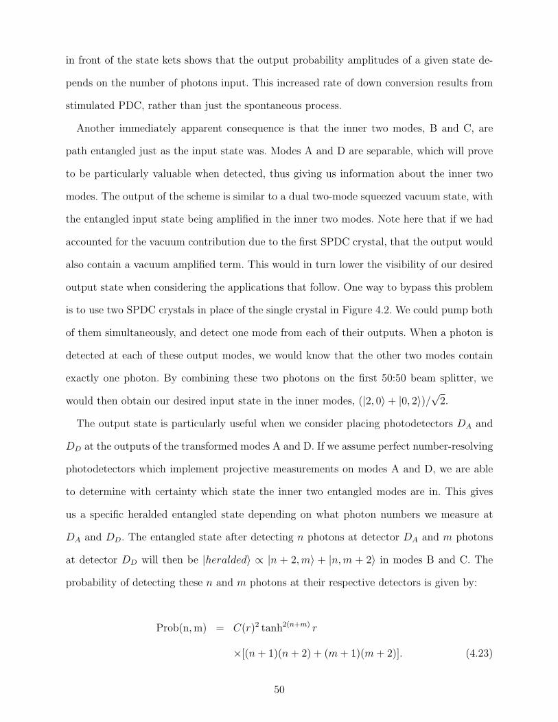
in front of the state kets shows that the output probability amplitudes of a given state de-

pends on the number of photons input. This increased rate of down conversion results from

stimulated PDC, rather than just the spontaneous process.

Another immediately apparent consequence is that the inner two modes, B and C, are

path entangled just as the input state was. Modes A and D are separable, which will prove

to be particularly valuable when detected, thus giving us information about the inner two

modes. The output of the scheme is similar to a dual two-mode squeezed vacuum state, with

the entangled input state being amplified in the inner two modes. Note here that if we had

accounted for the vacuum contribution due to the first SPDC crystal, that the output would

also contain a vacuum amplified term. This would in turn lower the visibility of our desired

output state when considering the applications that follow. One way to bypass this problem

is to use two SPDC crystals in place of the single crystal in Figure 4.2. We could pump both

of them simultaneously, and detect one mode from each of their outputs. When a photon is

detected at each of these output modes, we would know that the other two modes contain

exactly one photon. By combining these two photons on the first 50:50 beam splitter, we

would then obtain our desired input state in the inner modes, (|2, 0〉+ |0, 2〉)/√

2.

The output state is particularly useful when we consider placing photodetectors DA and

DD at the outputs of the transformed modes A and D. If we assume perfect number-resolving

photodetectors which implement projective measurements on modes A and D, we are able

to determine with certainty which state the inner two entangled modes are in. This gives

us a specific heralded entangled state depending on what photon numbers we measure at

DA and DD. The entangled state after detecting n photons at detector DA and m photons

at detector DD will then be |heralded〉 ∝ |n + 2,m〉 + |n,m + 2〉 in modes B and C. The

probability of detecting these n and m photons at their respective detectors is given by:

Prob(n,m) = C(r)2 tanh2(n+m) r

×[(n+ 1)(n+ 2) + (m+ 1)(m+ 2)]. (4.23)

50

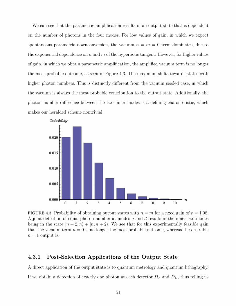
We can see that the parametric amplification results in an output state that is dependent

on the number of photons in the four modes. For low values of gain, in which we expect

spontaneous parametric downconversion, the vacuum n = m = 0 term dominates, due to

the exponential dependence on n and m of the hyperbolic tangent. However, for higher values

of gain, in which we obtain parametric amplification, the amplified vacuum term is no longer

the most probable outcome, as seen in Figure 4.3. The maximum shifts towards states with

higher photon numbers. This is distinctly different from the vacuum seeded case, in which

the vacuum is always the most probable contribution to the output state. Additionally, the

photon number difference between the two inner modes is a defining characteristic, which

makes our heralded scheme nontrivial.

FIGURE 4.3: Probability of obtaining output states with n = m for a fixed gain of r = 1.08.A joint detection of equal photon number at modes a and d results in the inner two modesbeing in the state |n + 2, n〉 + |n, n + 2〉. We see that for this experimentally feasible gainthat the vacuum term n = 0 is no longer the most probable outcome, whereas the desirablen = 1 output is.

4.3.1 Post-Selection Applications of the Output State

A direct application of the output state is to quantum metrology and quantum lithography.

If we obtain a detection of exactly one photon at each detector DA and DD, thus telling us

51

that n = m = 1, we know with certainty the entangled inner modes are in the state:

|inner〉 = (|3, 1〉+ |1, 3〉)/√

2. (4.24)

If this state (in modes B and C) is then incident on a beam splitter, using the transformations

[2],

b† → b† + eiθc†√2

, c† → b† − eiθc†√2

, (4.25)

and for θ = π we obtain the N = 4 N00N state:

|4, 0 : 0, 4〉 = (|4, 0〉+ |0, 4〉)/√

2 (4.26)

As discussed earlier, if this state is used to measure a path-length difference in a Mach-

Zehnder interferometer, it achieves a doubling in sensitivity compared to the standard shot-

noise limit [22]. We can easily see this since a coherent state with average photon number

n = 4 will reach the shot-noise limited phase-sensitivity of:

∆φ =1√n

=1√4

=1

2. (4.27)

However, since N00N states reach the Heisenberg limit, this four photon N00N state will

achieve a phase-sensitivity of:

∆φ =1

N=

1

4. (4.28)

Regarding use as a source for quantum lithography, proposed by Boto et al [4], 4-photon

N00N states are predicted to achieve interference patterns of the form 1 + cos(8φ), where

the phase φ corresponds to translation along the substrate at the interference plane [4].

This corresponds to a four-fold improvement in resolution compared to the classical case, for

which the pattern is of the form 1 + cos(2φ).

Optimizing the gain r such that we obtain the highest probability of obtaining a measured

output state of n = m = 1 gives a quantatative prediction for how often the desired state

for quantum metrology and lithography will be heralded. The optimal value is r = 0.66.

52

FIGURE 4.4: Probabilities of obtaining n and m photon states for fixed r = 1.08. The mostlikely joint photodetection at detectors DA and DD is when each mode contains only onephoton. The vacuum n = m = 0 term is the top diagonal term, and is not visible becausethe n = m = 1 term is more probable. A joint photodetection of n = m = 1 leads to theentangled state |3, 1〉+ |1, 3〉 between modes b and c, which when incident on a beam splitterleads to the N = 4 N00N state |4, 0〉+ |0, 4〉.

However, we are also able to find values of gain such that the n = m = 1 output state is more

likely to occur than the vacuum or any other n = m output. This is due to the output state

dependence on the number of photons in the modes, which is different from standard two-

mode squeezed vacuum, as previously mentioned. In spontaneous PDC, the most probable

outcome is always the vacuum contribution. Figure 4.4 shows the probabilities of obtaining

a measurement of n and m at the two detectors. The diagonal values are where n = m. The

inability to see the n = m = 0 term is due to the entanglement-seeding of the two OPAs.

The value of gain in this plot is r = 1.08, which is easily obtainable experimentally [20, 87].

Comparing the probabilities of obtaining the N = 4 N00N state to that of a typical linear

optics based scheme [59], we find that the dual OPA scheme produces the desired state more

53

frequently. In Reference [59] the N = 4 N00N state is probabilistically produced 3/64 of the

time. Our state produces the same state at approximately 5 times that rate. This is due to

the fact that the linear optical scheme relies on an input state of |3, 3〉, whereas our scheme

requires that each crystal produces the state |1, 1〉, which is much more likely for OPAs. Also,

our scheme is able to minimize vacuum contributions and shift the maximum probability to

higher photon number, as mentioned before, and as seen in Figure 4.3 and Figure 4.4.

4.3.2 Quantum Key Distribution Scheme Based on StimulatedParametric Down Conversion

One immediate consequence of the photon number difference in the two inner modes of the

output state applies to quantum cryptography. We imagine detecting n photons at DA and

m photons at DD. If we have perfect number resolving detectors, any time we measure n = m

we have the inner mode entangled state:

(|n+ 2, n〉+ |n, n+ 2〉)/√

2 (4.29)

To begin the QKD protocol, photodetector measurements at DA and DD are announced

publicly, while photon number measurements afterwards on modes B and C by two par-

ties (Alice and Bob) will be perfectly correlated. The time-energy entanglement of the two

modes results in a violation of the classical separability bound of the joint time and energy

uncertainties (∆EB,C)2(∆tB,C)2 ≥ ~2 [6, 8]. This type of entanglement is exploited to create

a one-time pad. A setup analogous to the experiment carried out by Howell’s group can

then be implemented [8]. In their scheme arrival times of photon pairs created from SPDC,

which are highly correlated, are used to create a cryptographic key. A time-bin setup is used

in order to ensure that detections at both Alice and Bob’s positions are due to the same

SPDC pair. This discretization of continuous-variable entanglement has been implemented

experimentally [8].

In my scheme, the number difference between the two modes, as well as the time-energy

entanglement is exploited, in order to create a key. After the values measured at DA and

54

DD are publicly announced, one of each of the remaining modes is sent to Alice, and the

other to Bob. Each of them then makes a photon number measurement on the mode they

have received. The analogy to Howell’s experiment is that Alice and Bob must implement

a time-bin system in order to ensure that the measurements they are making are on modes

produced from the same event.

For simplicity, consider only the cases when detectors DA and DD measure one photon

each, such that n = m = 1. The state will then be (|3, 1〉 + |1, 3〉)/√

2. Alice and Bob must

decide (publicly) beforehand that if, for example, Alice makes a measurement resulting in

one photon, and thus Bob the three photons, the resulting bit will be zero. If Alice makes a

measurement and obtains the three photon state, and Bob the single photon, the resulting

bit will be a one. The measurement outcomes of which mode (and correspondingly which

person) contains the single or three photon state, will be completely random from run-to-run.

Repeating the process many times will then result in a shared string of bits, corresponding

to a one-time pad key. Note here that noise-free photon number-resolving detectors with up

to 88% efficiency have been experimentally demonstrated at NIST [88]. However, imperfect

photodetectors have also been shown to provide useful reconstruction of photon-number

distributions as well [89].

The security of the system is established in a manner analogous to Howell’s experiment;

namely, Alice and Bob’s measurement devices must consist of a Franson interferometer

[68, 70]. This detection scheme requires that Alice and Bob each use an unbalanced Mach-

Zehnder interferometer. Each time they choose to make a measurement using the Franson

interferometer, they will be able to see coincidence fringes between their photon counts,

exactly the same as in Section 2.3.2. It has been shown that the Franson fringe visibility

corresponds to a Bell-type inequality, which allows for detection of an eavesdropper if there

is a reduction in the fringe visibility [8, 68]. The events in which Alice and Bob choose not

to make measurements with their interferometers may then be used to create the one-time

pad.

55

4.4 N00N State-Seeded Nonlinear Crystals

We have seen that N00N states reach the Heisenberg limit when used interferometrically to

measure phase differences between two paths, which is more sensitive than the classical shot-

noise limit. These states also write lithographic patterns that scale as 1+cos 2Nφ, where N is

the number of photons in the N00N state, which oscillate faster than allowed by the classical

Rayleigh diffraction limit. However, in real world situations, specifically in interferometry,

N00N states have been shown to be very sensitive to losses [62, 63]. N00N states perform

worse than the shot-noise limit when any significant amount of loss is present, which would

certainly be the case in a realistic interferometric scheme through the atmosphere.

Due to this sensitive dependence on loss, other states have been investigated in order

to find a more robust two-mode state that will still beat the shot-noise limit. Recently, a

colleague of mine has introduced states of the form 1√2(|M,M ′〉 + |M ′,M〉), (which we call

the MM’ state), which have been shown to be more robust than N00N states when loss

is present, while still beating the shot-noise limit [64]. Effectively, these states achieve the

equivalent phase sensitivity of a N00N state where N in the N00N state corresponds to the

photon number difference between the two modes in the MM’ state (|M-M’|). Qualitatively,

one can understand the N00N state sensitivity on loss by realizing that a loss of one photon

effectively corresponds to a measurement of a photon in the given mode, thus giving us

essentially full information about the state. If a photon is lost from one mode, we know that

the state is such that the N photons are in that mode, and zero photons are in the other

mode. However, in the MM’ state, as long as M ≥ 1 and M ′ ≥ 1, a loss of one photon will

not give full information about the state of the system, since each mode has at least one

photon in it.

I have realized a MM’ state generator scheme, involving two optical parametric amplifiers

and a N00N state input. Though it is difficult to create N00N states of large N , once an

efficient scheme is developed to create them, the setup that follows will effectively allow

them to be converted into the more robust MM’ states. The setup of the scheme is similar

56

FIGURE 4.5: Scheme for creating MM’ states. Two optical parametric amplifiers are seededsuch that a maximally path-entangled N00N state is input into modes B and C, while modesA and D are left as vacuum input. Not shown is the laser which is to pump both of thenonlinear crystals. Detectors DA and DD are present at the output of modes A and D, whichallow for heralded creation of states of the form |M,M ′〉+ |M ′,M〉.

to that of the previous section. Figure 4.5 shows a diagram of the scheme. The inner two

modes, B and C, are seeded with a N00N state while the outer two modes A and D are left

as vacuum. Similar to the previous section’s calculation, we assume the two OPAs have the

same squeezing parameter ξ = reiφ, and are both pumped with a phase-locked laser. OPA

I transforms modes A and B while OPA II transforms modes C and D. The total input is

then:

|input〉 =1√2

(|0, N, 0, 0〉+ |0, 0, N, 0〉). (4.30)

The optical parametric amplifiers then transform the four modes, and we are left with the

output state:

|output〉 =1√

2(N !)

N∑k=0

∞∑n=0

∞∑m=0

CN,kCm,n

×[κn|n− k, n− k +N,m,m〉+ κm|n, n,m− k +N,m− k〉]. (4.31)

57

We can see that the N00N state in the inner modes is amplified by each of the two OPAs,

but by different amounts corresponding to the sums over n and m. The factors out front are:

CN,k =N !

(N − k)!k!(cosh r)N−k(e−iφ sinh r)k (4.32)

Cm,n =1

cosh2 r(eiφ tanh r)n+m (4.33)

and

κn =

√(n− k +N)!√

(n− k)!. (4.34)

Now, if we again have detectors DA and DD at the output of modes A and D, respectively,

we may again obtain a heralded state. If we obtain a measurement of m′ photons at mode

A and n′ photons at mode D, the heralded output state in the inner two modes is then:

|heralded〉 ∝ |N + n′,m′〉+ |n′, N +m′〉. (4.35)

If, for example, we obtain a measurement of n′ = m′ ≡M ′, we can simply relabel the photon

numbers such that N +m′ →M to realize the heralded state is of the form:

|heralded〉 ∝ |M,M ′〉+ |M ′,M〉. (4.36)

Thus, if we detect n′ = m′ photons at the output of modes A and D, we are left with

a MM’ state in the inner modes B and C. This state may then be used for more practical

interferometry, and will beat the shot-noise limit so long as M 6= M ′. The larger the difference

in photon number between the two modes, the larger the shot-noise limit will be violated.

Thus, I have shown that if a N00N state scheme is created to effectively produce N00N

states, this scheme will straightforwardly convert them into the more robust MM’ states.

4.5 ChARM and Stimulated Parametric Down

Conversion

I began the setup of ChARM, the Correlated pHoton Absolute Radiometric Measurement

experiment, while at Northrop Grumman Aerospace Systems with the help of Dr. Jerome

58

Luine. ChARM is set to be an extension of a previous experiment done at NIST [39, 40].

The core of the experiment relies on stimulated parametric down conversion, and has a

significant application to radiometry, specifically on-satellite systems where calibration is

currently necessary.

We have seen that seeding nonlinear crystals with non-vacuum inputs will increase rates

of down converted photons. We will now examine some benefits of this in more depth. Using

the formula for spectral radiance [40]:

L(λ) =hc2

λ5〈n〉, (4.37)

where h is Planck’s constant, c is the speed of light, λ is the wavelength of light, and n is

the average number of photons per mode being measured. This quantity is a measure of the

amount of light emitted from a source at a given wavelength. In the quantum mechanical

sense, we can view the expectation value of n as the number of photons in that specific mode.

That is, the number of photons emitted in the given spatial mode at the wavelength λ we

are looking at.

Now, looking again at down conversion, we again use the output mode operators resulting

from transformations of the input modes:

a→ S(ξ)a0S†(ξ) = a0 cosh r + b†0e

iφ sinh r (4.38)

a† → S(ξ)a†0S†(ξ) = a†0 cosh r + b0e

−iφ sinh r (4.39)

b→ S(ξ)b0S†(ξ) = b0 cosh r + a†0e

iφ sinh r (4.40)

b† → S(ξ)b†0S†(ξ) = b†0 cosh r + a0e

−iφ sinh r. (4.41)

Calculating the average number of photons in each output mode straightforwardly results

in:

〈a†a〉 = 〈na〉 = na = 〈a†0a0〉 cosh2 r + 〈b0b†0〉 sinh2 r = na0 cosh2 r + (1 + nb0) sinh2 r (4.42)

〈b†b〉 = 〈nb〉 = nb = 〈b†0b0〉 cosh2 r + 〈a0a†0〉 sinh2 r = nb0 cosh2 r + (1 + na0) sinh2 r, (4.43)

59

by way of the fact that [a†, a] = 1 and [b†, b] = 1. Here na0 and nb0 correspond to the number

of photons input to the signal and idler modes (a and b), respectively. Now if we have no

photons input to either mode a or b, then the output number of photons in mode a will be

[40]:

na(nb0 = 0) = (0) cosh2 r + (1 + 0) sinh2 r = sinh2 r, (4.44)

which corresponds to amplification of the vacuum due to spontaneous parametric down

conversion. Now, if we again have no input into mode a, but now do have an input source

of photons into mode b, then the output number of photons, again in mode a, will be [40]:

na(nb0 6= 0) = (0) cosh2 r + (1 + nb0) sinh2 r = (1 + nb0) sinh2 r. (4.45)

Here we again see the effect of stimulated down conversion by way of the fact that the output

depends on the number of photons input to the system. Taking the ratio of the number of

output photons in mode a when mode b has a nonzero input to the output number of photons

in mode a when there is no input into mode b, we arrive at the formula [40]:

na(nb0 6= 0)

na(nb0 = 0)=

(1 + nb0) sinh2 r

sinh2 r= 1 + nb0 . (4.46)

Now, this ratio allows us to calculate the number of photons input into mode b by measuring

the output number of photons in mode a. To do this, we simply measure the number of

photons output in mode a with the input source into mode b turned off, as well as with it

turned on. Then, taking this ratio and subtracting one, we arrive at the total number of

input photons into mode b by measuring its down converted pair’s photon mode. From the

equation for spectral radiance, as long as we know the wavelength of the light in mode b,

we are able to calculate the input source’s (to that mode) radiance. This process shows that

a nonzero seed in one mode will increase the rate of down conversion, which we saw in the

first section in this chapter. Thus, this may be viewed as an increase in the gain factor by

having a nonzero seed, which we are measuring over a period of time. Then, without the seed

60

source, we are measuring the gain of the spontaneous down conversion process. This ratio is

what gives us the radiance of the source that I mentioned previously in this paragraph.

In order to see how this ties together with stimulated down conversion, consider the two-

photon seeded case. We have an input of:

|input〉 = |0, 2〉 =1√2!b†2|0, 0〉. (4.47)

Using the procedure mentioned in section 4.1 (using the Taylor series expanded version of

the evolution operator corresponding to the Type I down conversion regime), we see that

the output will then be:

|output〉 =1√2!Sb†2|0, 0〉 =

1√2!

(1− ξa†b† + ξ∗ab)b†2|0, 0〉 = |0, 2〉 −√

3ξ|1, 3〉. (4.48)

Now, consider the case corresponding to three photons input into mode b, such that:

|input〉 = |0, 3〉 =1√3!b†3|0, 0〉. (4.49)

Similarly, we will then obtain an output state of:

|output〉 =1√3!Sb†3|0, 0〉 =

1√3!

(1− ξa†b† + ξ∗ab)b†3|0, 0〉 = |0, 2〉 −√

4ξ|1, 4〉. (4.50)

Finally, recall that unseeded, spontaneous parametric down conversion corresponding to this

thought experiment will produce the output state |output〉 = |0, 0〉 − ξ|1, 1〉. Now we will

consider photon count measurements at the output mode a in each of the three scenarios

(two, three and no photon seeds in mode b). Due to the fact that the vacuum state in each

of the three outputs will not result in a photon count, these terms may all be neglected.

Thus, we are left with the three states that would correspond to the state we measure when

detecting a photon in mode a:

vacuum input: ξ|1, 1〉

two-photon input:√

3ξ|1, 3〉

three-photon input:√

4ξ|1, 4〉

61

We see that in each case, we are measuring one photon in mode a. However, the effective

gain is increased with the addition of each additional photon seeded into mode b, regardless

of the fact that we measure only mode a at the output. This increase in the down conversion

rate due to stimulated emission is the basis for the ChARM experiment. The second-order

susceptibility in front of each term is the same, so long as we use the same crystal, and will

therefore cancel when we look at the ratio of measurements taken with the input to mode

b turned off and on. Thus, we are left with the number of photons input into mode b (plus

one, as in the equation), which as mentioned can then easily be converted to the radiance of

the input source into that specific mode.

In order to see clearly that this method works, we will consider the examples above and

measurements of photon number in mode a in each case. Measuring the number of photons

in mode a at the output of the unseeded crystal case, we obtain:

(〈0, 0| − ξ∗〈1, 1|)na(|0, 0〉 − ξ|1, 1〉) = (〈0, 0| − ξ∗〈1, 1|)a†a(|0, 0〉 − ξ|1, 1〉) = |ξ|2. (4.51)

Measuring the number of photons in mode a when we have two input photons into mode b,

we see:

(〈0, 2| −√

3ξ∗〈1, 3|)a†a(|0, 2〉 −√

3ξ|1, 3〉) = 3|ξ|2 (4.52)

Taking the ratio of the measurement with two photons input to vacuum input and subtracting

one, we find:

3|ξ|2

|ξ|2− 1 = 3− 1 = 2. (4.53)

Thus, the ratio of the measurements minus one gives us the total number of photons input

into mode b, simply by measuring mode a. In precisely the same manner, the case of mea-

suring photon number in the output of mode a when three photons are input to mode b, we

arrive at:

(〈0, 3| −√

4ξ∗〈1, 4|)a†a(|0, 3〉 −√

4ξ|1, 4〉) = 4|ξ|2. (4.54)

62

Again taking the ratio and subtracting one, we obtain:

4|ξ|2

|ξ|2− 1 = 4− 1 = 3. (4.55)

This again shows that by taking the ratio of the measurements and subtracting one we arrive

at the number of photons input to mode b.

There are a couple of advantages to making a radiance measure with this method. The

first is that no calibration source is needed whatsoever [40]. In a typical device used to

measure radiance, a blackbody source is needed in order to obtain an absolute radiance

measure of the source of interest. However, due to the fact that down conversion results in

perfect photon number correlations between the two output modes, we know that anytime

we count one photon in mode a, we have exactly one photon in mode b. So, when we make

the measurements with the input seed on and off, then calculate the ratio, we obtain an

absolute measurement of the number of input photons into the specific mode. There is

no need for a calibrated source to compare the radiance measurement to. One important

application of this benefit is to on-board satellite radiance measurement systems. Since it is

extremely difficult (if not impossible) to fix an apparatus on a satellite, calibrated sources

used in measurement devices on satellites must be very stable. If the source changes over

time in an unknown manner, this can lead to incorrect absolute measurements of a source the

satellite is measuring. However, if a stimulated parametric down conversion system is used,

as in ChARM, the need for a calibrated source disappears, likely increasing the stability and

lifetime of the measurement device on the satellite.

Another advantage of ChARM relates to the energy conservation and phase-matching

conditions imposed by down conversion. The down conversion process requires that ωp =

ωs + ωi. If we know the wavelength we are interested in of the source, in say the idler

mode, then we know at what wavelength we need to measure the corresponding signal mode.

Additionally, the spatial correlations between the signal and idler will determine where we

are to measure the specific wavelength in space. Thus, by moving our detector spatially, we

63

FIGURE 4.6: Simplified experimental setup for the ChARM experiment. A nonlinear crystalis pumped by a laser. One of the input modes (signal) is seeded with a source whose radianceis to be determined. A single photon counting module is placed at the output of the idlermode. Photon counts will be made with the signal source turned on and off.

are changing the signal mode we are measuring (that is, its wavelength) and are now able

to measure the radiance of the source at a different wavelength, again subject to the energy

conservation requirement. The advantage resulting from these constraints and correlations

is that we can measure the radiance of the idler source at wavelengths that are difficult to

measure, by measuring the corresponding signal mode at a wavelength that may be more

accessible. For example, we may have a pump and crystal setup such that when we are

measuring a signal mode of wavelength 725nm, the idler is out in the infrared at 4000nm.

Detectors in the visible are typically better and more efficient than IR detectors, thus allowing

for a more accurate measurement.

The NIST experiment was able to measure the absolute radiance of a source at wavelengths

out to just under 4.8µm with an accuracy of about 3% [40]. ChARM will be implemented

to hopefully reach uncertainties down to below 0.5% out to wavelengths approaching 18µm.

Initially, ChARM will utilize three separate nonlinear crystals, along with three different

wavelength pump beams, to reach these long wavelengths. A single-photon counting mod-

ule will be used to detect photons in the signal output mode in each different setup. The

experimental setup as shown in Figure 4.6 will be discussed more in the following section.

64

4.5.1 Realistic Experimental Setup and Improvements

The experimental setup of ChARM involves four major components. These are the nonlinear

crystal, the pump laser, the source to be measured and a single photon counting detector. One

major difficulty in making the ChARM measurement will be the geometry of the experiment.

Since we are trying to measure the down converted photons at one given wavelength at a

time, the spatial placement of the single photon counting detector is extremely important.

Moreover, the spatial overlap of the source beam (beam whose radiance is to be determined)

with the pump beam is both difficult to align as well as a major source of error if improperly

setup. A photon from the source beam will only contribute to stimulated down conversion if

it overlaps spatially with the pump beam inside the crystal, is of the appropriate polarization,

and will only stimulate into the specific spatial signal and idler output modes. Thus, overlap

of the two beams inside the length of the crystal must be maximized, as in [40].

The general experimental setup for ChARM is shown in Figure 4.6. The setup is such

that the angle the source beam and the pump beam make with one another is as constant

as possible. The pump laser and the source beams will meet at the input crystal face. In

order to maximize down conversion rates at various wavelengths, the crystal will be mounted

on a 6-axis mount. Each different wavelength to be measured will require a different input

angle of the pump relative to the input crystal face. Additionally, the photon counting

detector at the output idler mode will also need to be varied in position (angle) each time

a different wavelength is being examined. This allows for a single crystal to be used for a

variety of radiance measurements at different wavelengths by simply tilting the crystal and

repositioning the detector.

Another consideration taken into the experimental design is the bandwidth of the source

to be measured. This bandwidth will effectively determine the angular range of output stim-

ulated down conversion photons. In order to make an accurate measurement, we will need

to place a narrow linewidth filter after the source, before it enters the nonlinear crystal.

Additionally, a pinhole will be placed in the the output idler mode’s path to select out the

65

appropriate spatial mode before the single photon counting detector. Due to the fact that

all optics to be used are not ideal, there will be losses associated with each one. In order

to stimulate down conversion into the appropriate modes, the source must also be polarized

parallel to the output signal and idler modes. Hence the need for a half-wave plate before

the filter in the source’s path prior to the crystal. In order to compensate for the losses due

to the optics before the crystal, we will make measurements of the ”source” as if it were

produced at the very last optic before it enters the nonlinear crystal. In order to determine

the absolute accuracy of ChARM’s measurements, we must make a standard radiometric

measurement with a known source. To do this we will place the known source at the position

of the last optic before the crystal input face. This will give us an absolute measure of the

radiance of the ”source” as mentioned, namely the source being the output from the last

optic. Thus, we will only need to measure the losses coming from the optics after the crystal,

which should improve the overall accuracy of the measurement.

The crystals we will be using are Lithium Iodate (LiIO3), Silver Gallium Sulfide (AgGaS2)

and Silver Gallium Selenide (AgGaSe2). LiIO3 will allow us to make measurements of the

source’s radiance at wavelengths from 2.5µm to 4.5µm. AgGaS2 will allow for wavelengths

from 5µm to 9µm, and AgGaSe2 from 10µm to 18µm. A 532nm laser will be used to pump

the Lithium Iodate crystal, while a 1550nm laser will pump the Silver Gallium Selenide

crystal and frequency doubled to 725nm to pump the Silver Gallium Sulfide crystal.

The pump beam for the Lithium Iodate experiments is a Verdi V6 diode-pumped solid-

state laser. A diode laser is used to pump a vanadate (NdYVO4) crystal which is used as the

gain medium to produce 1064nm laser light. Then a Lithium Triborate (LBO) crystal is used

for second harmonic generation, resulting in single-mode 532nm laser light. The laser head

is cooled by being placed on a plate stand through which chilled water at 18C circulates.

The output laser operates from 10mW up to a maximum of 6W . The beam is very nearly

Gaussian, with an M2 value of less than 1.1. The 1550nm laser to be used for the Silver

Gallium crystals is similar in spec and also single-mode.

66

4.5.2 Calculated Spontaneous Parametric Down ConversionRates

One important theoretical contribution I made to ChARM was to calculate the expected

rate of spontaneous parametric down conversion events in the various setups involved. This

was done to decide the appropriate sizes of the crystals we would end up needing to order.

Larger crystals are more expensive, but too small of crystals may not produce enough down

conversion events. Though at first a seemingly trivial task, it proved to be quite the opposite.

There has been research looking into rates of spontaneous parametric down conversion.

However, until recently these have all considered a total rate of down conversion efficiency

[90]. That is, the overall rate and/or probability of a photon in the pump beam being down

converted into two other photons, regardless of which two modes they are down converted

into. While this may be useful when comparing various general SPDC setups, in which

different crystals and pumps are used, it only serves to give an estimate of the rate of total

down conversion into all of the various modes allowed by the phase-matching conditions. In

our experiment, we are concerned only with the rate of down conversion in the specific idler

mode that we are measuring, and therefore, its corresponding signal mode. Modes at other

spatial and frequency locations are not nearly as important, as we are not measuring them.

Recently, a group in Singapore published a paper discussing absolute emission rates of

down conversion into single transverse Gaussian modes [91]. This is precisely what we are

interested in when discussing down conversion rates in ChARM. We have a Gaussian pump

beam and assume the output modes we are looking at to be Gaussian. They found that the

absolute rate was [91]:

R =4χ(2)2PpLω

2p

3π2npnsniε0c2W 2p (1 + cos θ2

s + cos θ2i )(ni cos θi − ns cos θs)

S, (4.56)

where Pp is the pump power, L is the crystal length, ns is the signal mode’s index of refraction,

Wp is the pump beam waist size, θi is the angle the idler mode makes relative to the pump,

and S is the ”spectral integral.” The waists of all three modes are assumed to be the same for

67

simplicity. The spectral integral contains dependence regarding the walk-off of the beams. It

depends on the walk-off parameter [91]:

Ξ =L

2[sin2 θsW 2s

+sin2 θiW 2i

− (sin 2θsW 2s

− sin 2θiW 2i

)2/(4

W 2p

+cos2 θsW 2s

+cos2 θiW 2i

)]1/2 (4.57)

I have written two Mathematica notebooks, one to calculate the walk-off parameter and

the other to then calculate the total rate of SPDC into a given mode using the equations

derived in [91]. Using these, along with a LabView program written by Migdall at NIST

[92], and our specific experimental setups, I calculated the rates of spontaneous parametric

down conversion we will expect to see in ChARM. The parameters that were varied are the

angles between the signal and the pump beam as well as the idler and the pump beam,

the indices of refraction of the signal, idler and pump modes at the given wavelengths and

angles of propagation, and finally, the angle between the pump and the input face of the

crystal. I made calculations at the various wavelengths (and thus, various modes) for each

nonlinear crystal to be used in the experiment. Again, in order to look at various wavelengths

corresponding to different modes, we see that the angle between the pump beam and the

input face of the crystal is rotated. Additionally, I varied the crystal length of the two Silver

Gallium crystals in order to find a (monetarily) realistic size that would still produce down

conversion rates of ≥ 100, 000s−1. A size of 5mm in length for both crystals seems to produce

sufficient rates for the ChARM experiment. These spontaneous parametric down conversion

rates are listed in the following four figures.

68

FIGURE 4.7: Relevant data for LiIO3 SPDC rate calculation. ”d” is the effective nonlinearityand ”Theta tilt” is the angle between the pump beam and the input face of the crystal.Pump wavelength is 532nm, power is 6W, and beam waist is 1.125mm.

69

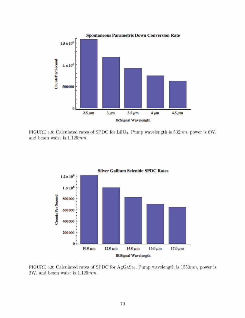
FIGURE 4.8: Calculated rates of SPDC for LiIO3. Pump wavelength is 532nm, power is 6W,and beam waist is 1.125mm.

FIGURE 4.9: Calculated rates of SPDC for AgGaSe2. Pump wavelength is 1550nm, power is2W, and beam waist is 1.125mm.

70

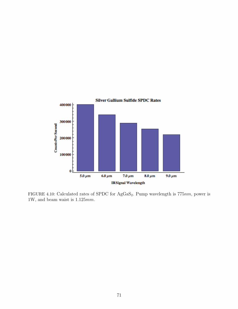
FIGURE 4.10: Calculated rates of SPDC for AgGaS2. Pump wavelength is 775nm, power is1W, and beam waist is 1.125mm.

71

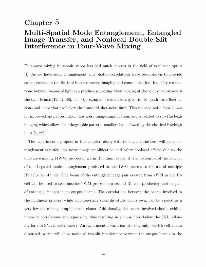
Chapter 5Multi-Spatial Mode Entanglement, EntangledImage Transfer, and Nonlocal Double SlitInterference in Four-Wave Mixing

Four-wave mixing in atomic vapor has had much success in the field of nonlinear optics

[1]. As we have seen, entanglement and photon correlations have been shown to provide

enhancements in the fields of interferometry, imaging and communication. Intensity correla-

tions between beams of light can produce squeezing when looking at the joint quadratures of

the twin beams [45, 47, 48]. The squeezing and correlations give rise to quadrature fluctua-

tions and noise that are below the standard shot-noise limit. This reduced noise floor allows

for improved optical resolution, less noisy image amplification, and is related to sub-Rayleigh

imaging which allows for lithographic patterns smaller than allowed by the classical Rayleigh

limit [4, 22].

The experiment I propose in this chapter, along with its slight variations, will show en-

tanglement transfer, low noise image amplification and other nonlocal effects due to the

four-wave mixing (4WM) process in warm Rubidium vapor. It is an extension of the concept

of multi-spatial mode entanglement produced in one 4WM process to the use of multiple

Rb cells [45, 47, 48]. One beam of the entangled image pair created from 4WM in one Rb

cell will be used to seed another 4WM process in a second Rb cell, producing another pair

of entangled images in its output beams. The correlations between the beams involved in

the nonlinear process, while an interesting scientific study on its own, can be viewed as a

very low noise image amplifier and cloner. Additionally, the beams involved should exhibit

intensity correlations and squeezing, thus resulting in a noise floor below the SNL, allow-

ing for sub-SNL interferometry. An experimental variation utilizing only one Rb cell is also

discussed, which will show nonlocal two-slit interference between the output beams in the

72

4WM process, resulting from the large quadrature entanglement produced.

Examining the ideal interaction Hamiltonian for off-resonant nondegenerate four-wave

mixing [45]:

HI = ~χ(3)(α2a†b† + α∗2ab), (5.1)

we are able to immediately see some various effects that will be discussed in this chapter,

by noticing how similar the Hamiltonian is to the down conversion process [2]. Note that

this interaction Hamiltonian is ideal, neglecting losses and assumes the undepleted pump

approximation. We see a slight difference from the down conversion Hamiltonian by the

presence of α2 rather than just α, which is due to the fact that two pump photons contribute

to the interaction. This Hamiltonian also neglects a cavity, so we are dealing with 4WM

in a vapor cell that is not inside a resonant cavity such that the pump beam only makes

one pass through the cell. Additionally, this Hamiltonian is a good approximation for the

non-degenerate 4WM process when the pump beam(s) is not precisely on-resonance with

the atomic transitions, such that we may neglect spontaneous emission and allow the atomic

medium to be characterized by its third-order nonlinear susceptibility χ(3).

5.1 Joint Quadrature Squeezing Via Four-Wave

Mixing

We have seen that squeezed light exhibits quadrature fluctuations below that of coherent,

or laser light. Due to the uncertainty principle, if one quadrature is squeezed below that of

a minimum uncertainty state (such as a coherent state, or the vacuum), the other quadra-

ture’s fluctuations increase. However, it is also possible for squeezing to exist between joint

quadratures of two light beams. Defining the quadrature operators Xa, Ya for beam ”a”

(probe beam) and Xb, Yb for beam ”b” (conjugate), we can realize the joint quadrature

operators [47, 48]:

X+ = (Xa + Xb)/√

2 (5.2)

Y− = (Ya − Yb)/√

2. (5.3)

73

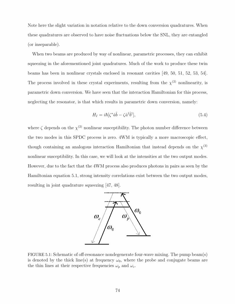
Note here the slight variation in notation relative to the down conversion quadratures. When

these quadratures are observed to have noise fluctuations below the SNL, they are entangled

(or inseparable).

When two beams are produced by way of nonlinear, parametric processes, they can exhibit

squeezing in the aforementioned joint quadratures. Much of the work to produce these twin

beams has been in nonlinear crystals enclosed in resonant cavities [49, 50, 51, 52, 53, 54].

The process involved in these crystal experiments, resulting from the χ(2) nonlinearity, is

parametric down conversion. We have seen that the interaction Hamiltonian for this process,

neglecting the resonator, is that which results in parametric down conversion, namely:

HI = i~[ζ∗ab− ζa†b†], (5.4)

where ζ depends on the χ(2) nonlinear susceptibility. The photon number difference between

the two modes in this SPDC process is zero. 4WM is typically a more macroscopic effect,

though containing an analogous interaction Hamiltonian that instead depends on the χ(3)

nonlinear susceptibility. In this case, we will look at the intensities at the two output modes.

However, due to the fact that the 4WM process also produces photons in pairs as seen by the

Hamiltonian equation 5.1, strong intensity correlations exist between the two output modes,

resulting in joint quadrature squeezing [47, 48].

FIGURE 5.1: Schematic of off-resonance nondegenerate four-wave mixing. The pump beam(s)is denoted by the thick line(s) at frequency ω0, where the probe and conjugate beams arethe thin lines at their respective frequencies ωp and ωc.

74

5.2 Multi-Spatial-Mode Entanglement in Four-Wave

Mixing

Entanglement produced in a SPDC type of setup is inherently multi-spatial-mode because

of the phase-matching conditions involved [92]. In order to extend this toward a macroscopic

beam and increase the gain, these crystals are typically placed in a resonator in order to

increase the effective nonlinearity. This device is called an optical parametric oscillator, due

to the resonant cavity [49, 50, 51, 52, 53]. However, due to effects when including the resonant

cavity, the multi-spatial-mode entanglement is lost and one is typically left with single-

spatial-mode twin beams [54]. Still, the twin beams will exhibit strong intensity correlations

when measuring the whole of each beam.

Recently, this single-spatial-mode problem has been overcome by use of another nonlin-

ear process, 4WM [46]. Lett’s group showed that the entanglement between the probe and

conjugate beams produced by the 4WM process in warm Rubidium vapor was multi-spatial-

mode and thus had the ability to contain entangled images. That is, subsections of each

beam contain photon number correlations with one another. Therefore, one can envision the

output beams containing an image, where individual parts of the image are correlated spatial

mode-to-spatial mode. It should be noted that due to the different energy level transitions,

the probe and conjugate beams are at different frequencies, separated by the ground state

sublevel energy difference. This process involves the conversion of two pump photons into one

probe and one conjugate photon, where the probe is the beam which seeds the Rb vapor. The

input conjugate mode was left as vacuum. Homodyne detection of the probe and conjugate

(output) beams was performed, with local oscillators produced in the same Rb cell, but at a

different spatial location. Joint quadrature squeezing was seen between the resulting probe

and conjugate beams. The multi-spatial-mode aspect of the process was demonstrated by

placing various images on the beam that produces the local oscillators and seeing squeezing

below the SNL.

75

Being multi-spatial mode, the 4WM process allows for imaging schemes. Entangled im-

ages have been produced via this process [46]. Rather than seeding both input modes with

vacuum, a beam with an image is input into the probe mode. Due to the photon number

correlations produced in the process, along with the multi-spatial mode aspect, the output

probe and conjugate beams both contain the input image (though the conjugate is just

that, the conjugate of the image). Again by making homodyne measurements on the output

modes, it has been shown that the various spatial modes of the images in the output beams

are entangled with one another. This process may be thought of as analogous to the stimu-

lated parametric down conversion process, where we introduce a non-vacuum seed. However,

we are now utilizing the multi-spatial mode aspect in order to produce images. One benefit

of the 4WM variation is that the gain is much larger than in parametric down conversion.

The next section describes a proposed experiment to utilize the multi-spatial mode entan-

glement in the 4WM process as seen in Figure 5.2.

FIGURE 5.2: Diagram of the entangled image transfer scheme.

76

5.3 Entangled Image Transfer via Four-Wave Mixing

Combining previous research involving seeded nonlinear optical effects with the 4WM in Rb

vapor work mentioned in the previous section leads to an interesting image transfer concept

[36, 46]. We have already seen that the single-photon seeded stimulated PDC process is an

example of the best possible quantum cloner [32, 33]. Another way to view these seeded PDC

schemes is as an amplifier [35, 83]. The input state is amplified in the sense that photons

in the same mode are added to the input (regardless of the input state). This proposed

experiment is a 4WM analogue of this, also allowing for imaging due to its multi-spatial

mode property.

The idea is to take one beam of the multi-spatial-mode entangled twin beams produced

in the 4WM process and using it to seed another 4WM process. This is then a realization

of image amplification and cloning (or transfer) of the seeding beam. Due to the seeding

of the second Rb cell with the entangled image, the two output beams produced will be

entangled, and both contain the original image from the first 4WM process. Additionally,

by measurement of the second output probe beam, and conditional readjustment of the

second cell’s pump beam, we should be able to obtain degenerate twin beams exhibiting

joint quadrature squeezing. These degenerate twin beams would be the conjugate beam

from the first cell and the conjugate beam from the second cell.

A schematic of the scheme is shown in Figure 5.2. First, the pump beam is split in order to

pump the first and second Rb cells, as well as create the local oscillators (LOs, as I will discuss

soon). The first Rb cell is pumped at the pump frequency and seeded with a probe beam

containing an image. The input conjugate beam will remain vacuum. As we have seen, the

output conjugate and probe beams will contain the entangled image from the probe seed [46].

The output probe beam will then be used to seed the second Rb cell, which is also pumped at

the pump frequency. The output (from the second cell) probe and conjugate beams will then

contain an entangled image resulting from the image of the probe seed. By examining the

three images produced we can see that this is a realization of image amplification and transfer.

77

This may be viewed as the amplification and/or transfer of the original entangled image to

the second output probe and conjugate beams. This initial experiment is a realization of low

noise image amplification and transfer, as we will be transferring the image on the initial

seed beam to three other beams. One nice aspect of this is that the two conjugate beams

produced, one from the first cell and one from the second, both contain the same image since

they are both conjugate beams. Additionally, they are frequency degenerate, so they will be

able to interfere with one another.

In order to show that entanglement exists between the first cell’s conjugate output beam

and the second cell’s output beams, homodyne detection will be necessary. This will be done

by producing local oscillators in the first Rb cell by splitting off part of the pump beam and

routing it into a spatially separated (from the 4WM beams) region of the first Rb cell, as

in [46]. The probe and conjugate beams produced from this interaction will then serve as

the local oscillators for the homodyne detection setups. The first conjugate beam and the

LO at its frequency will be mixed on a beam splitter, while varying the LOs phase with

a piezoelectric actuated mirror. Photodetectors will measure the intensity difference at the

two output ports. A homodyne measurement of the other beam we are interested in (the

conjugate beam produced at the second Rb cell) will be performed by mixing it with the LO

at its frequency (same as the first conjugate beam) at another beam splitter, and recording

the intensity difference at the output ports. Finally, the intensity sum and difference of

the two homodyne measurement outputs will be measured by spectrum analyzers. If we

perform homodyne measurements (and sum/difference measurement) on both of the beams

produced at the second Rb cell, we would immediately see squeezing and sub-shot noise

joint quadrature fluctuations. Placing multiple images on the beam that produces the LOs

and repeating the measurement procedure would provide proof of the multi-spatial-mode

structure of the resulting correlations.

It is likely that in order to see squeezing and show that the entanglement has been amplified

to contain both conjugate beams, we would need to use feedback. First we would perform the

78

measurement process described above with the conjugate beams produced from both cells. If

the joint quadrature noise is above the SNL, we would need to adjust the pump power at the

second cell in order to minimize spontaneous emission and maximize the stimulated emission

due to the probe seeding. Proper adjustment and reapplication of the measurement on the

two conjugates should provide sub-shot noise fluctuations on their joint quadratures. This

process can be repeated with the first cell’s conjugate beam and the second cell’s probe beam,

in order to show an entanglement transfer to all three beams. The degree of entanglement

will likely be decreased between the final output beams and the beams produced from the

first Rb cell. This is again in analogy with the cloning and entanglement amplification due

to stimulated parametric down conversion, in which the entanglement decreased due to noise

arising from vacuum amplification. However, due to the fact that the two conjugate beams

are frequency degenerate, and contain the same image, useful applications still abound even

if the entanglement between them is minimal.

The experiment should initially show the amplification of an entangled image. That is,

the image from the initial probe beam, which is transferred to the first probe and conjugate

beams which are entangled (after the first Rb cell) to be amplified in the sense that the image

will be imprinted on the final probe and conjugate beams (after the second Rb cell). Thus,

the image from one seed beam and transferred it to a total of three beams. The application

of this would be related to the ”no-noiseless amplification” theorem, which is essentially the

(semi) classical analogue to the quantum ”no-cloning” theorem. Previous work with quantum

seeding of optical parametric amplifiers and nonlinear crystals, such as single-photon seeded

nonlinear crystals, are examples of the nearest quantum schemes to perfect cloning as we

saw in chapter 4 (though not perfect, as mandated by the no-cloning theorem) [32, 33, 36].

This non-vacuum seeding of Rb vapor and amplification of the image on the seeding beam

is, in a sense, an extension of my previous quantum-seeding theory to 4WM [36]. Namely,

the noise added in the image amplification process is expected to be minimal (again nonzero,

as mandated by the no-noiseless amplification theorem).

79

Additionally, one should be able to show that the entanglement between the first probe and

conjugate beams will be transferred to the probe and conjugate beams produced in the second

Rb cell. This will likely be a more difficult task, and require careful feedback measurements

of the final output probe. In the low-gain limit this process mimics the parametric down

conversion scenario. If a single photon is input in the probe mode, it is analogous to the

single-photon seeded dual crystal schemes, in which the various output modes from the two

crystals are entangled (pending a down conversion event occurring) [35, 83]. This can be

seen immediately by noting the similarities between the interaction Hamiltonians for the

parametric down conversion and 4WM processes. A calculation may be carried out in an

analogous manner to that in section 4.1. We take the input to the second Rb cell to be a

single photon in the signal mode a. The output would then be:

|1, 0〉+ ξ2√

2|2, 1〉, (5.5)

where ξ depends on the χ(3) nonlinear susceptibility, interaction time and pump beam power.

Thus, we can see that again the input signal mode photon is cloned in a similar manner to

the stimulated down conversion process. The detection of an output photon in mode a of

the state in equation 5.5 gives us knowledge about the state in the conjugate mode b. Due

to the multi-spatial mode aspect of this process, We may then draw a conclusion about

which spatial mode the conjugate photon to the signal seed photon is in. In this sense, we

are transferring the correlations to multiple beams. Additionally, if one can extend this to

show macroscopic squeezing between the two conjugate beams produced in the experiment,

it should be straightforward to input these beams into an interferometer and show sub shot-

noise phase estimation. This is due to the advantageous fact that the two conjugate beams

are necessarily frequency degenerate in the setup. Beating the shot-noise limit is an extremely

desirable result which is applicable to LIDAR and other sensor systems as we have seen [22].

A direct contingency that would apply if unexpected results are obtained such as not

being able to show macroscopic joint quadrature squeezing between the two conjugate beams

80

produced would be back to imaging. The transfer of the image to two frequency degenerate

beams will still be an example of very low noise amplification. In a sense, this is a macroscopic

version of ideal (not perfect) cloning. An additional application for entangled images and

entangled image transfer is to quantum key distribution [8]. We saw in chapter 4 that spatial

entanglement along with time-energy entanglement can be used on the single photon level to

produce large alphabet QKD [6, 7, 8]. Macroscopic, many-spatial-mode entanglement would

likely allow for higher key distribution rates, and may even allow for the future possibility

of multi-user QKD. This would be realized as an extension of spontaneous parametric down

conversion QKD experiments to the large quadrature entanglement produced in seeded 4WM

experiments.

Another proposed experiment is discussed in the next section, involving a nonlocal double

slit setup as seen in Figure 5.3.

FIGURE 5.3: Diagram of the nonlocal double slit experiment. Superposition of masks one andtwo is a double slit. Coincidence detection of probe and conjugate beam intensities will resultin a double slit interference pattern. This will result from the strong intensity correlationsbetween the various spatial modes of the two output beams.

81

5.4 Nonlocal Double Slit Interference Via Two Warm

Rubidium Vapor Cells

Due to the multi-spatial mode structure of the output probe and conjugate beams produced

via the 4WM process, a variety of imaging experiments may be constructed. Additionally, the

entanglement between the two output beams may be exploited, once again, in an analogous

way with respect to stimulated down conversion. The main point behind the proposed exper-

iments in this section will be to further explore the similarities between down conversion in

nonlinear crystals and 4WM in atomic vapor. However, they also have various applications

to sub-shot noise imaging, again similar to applications of down conversion, though in a

higher gain regime.

To begin the discussion on these various imaging schemes, let us review some interesting

properties of spontaneous and stimulated parametric down conversion. This is done in order

to gain some intuition about the 4WM process’s analogous properties and applications.

It has been shown that the angular spectrum and intensity profile of the pump beam is

transferred to the signal and idler beams in the SPDC process [94]. The simplest way to see

this is by the realization that a pump photon with a given ~k will down convert into specific

spatial modes only, as allowed by the phase-matching and energy conservation conditions as

controlled by the crystal cut [92]. We discussed this very briefly in section 4.5 when trying

to understand the importance of the various geometries in the ChARM experiment design

and setup. Mathematically, we may see this by examining slightly less ideal derived output

state of the SPDC process, in which we assume the pump beam has some spatial variation

or angular spectrum [94]:

|ψ〉 = |0〉|0〉+ C

∫d~ks

∫d~kiΦ(~ks, ~ki)sinc

1

2(ωs + ωi − ωp)t|1〉|1〉 (5.6)

where the function Φ is defined as:

Φ(~ks~ki) =

∫d~qpv(~qp)(

ωpωsωin2pn

2sn

2i

)1/2

3∏m=1

sinc1

2(ks + ki − kp)mLm. (5.7)

82

Here, C is a constant, ~q is the transverse component of the pump wave vector, nm is the

refractive index of the corresponding mode in the crystal, Lm is the length of the crystal in

the given direction, and v(~qp) is the angular spectrum of the pump beam. Though this may be

simplified by making various approximations, the important thing to note is that the angular

spectrum of the pump beam is transferred to the output signal and idler modes. Note that

this SPDC output state is more complicated than the assumed output in previous sections.

This is because in the previous sections we were not concerned with the spatial profile of

the pump by assuming it was spatially uniform, and assumed it was an infinite plane wave.

The equation above is applicable when discussing the multi-spatial mode property of the

SPDC output, as we are able to manipulate it by placing images on the pump. The previous

chapters’ SPDC outputs were sufficient for the discussions therein, as we were concerned

only with certain aspects of the SPDC process, such as photon number correlations between

two single modes.

Coincidence count measurements between the signal and idler output modes of the afore-

mentioned state results in fourth-order interference patterns. By making a coincidence mea-

surement, which is proportional to:

〈ψ|a†b†ab|ψ〉, (5.8)

it can be shown that the angular spectrum of the pump again appears (more precisely, its

Fourier transform). An experiment was then done to show exactly this effect [94]. The group

placed a double slit in the pump’s path before the crystal, then made coincidence detection

measurements at the output signal and idler modes. By varying the position of the detectors

in these modes, they were able to see a double slit interference pattern when coincidence

counting between the signal and idler beam output positions. This is related to the previous

section on 4WM in that it is an example of image transfer from one beam to a pair of

entangled ”beams” (beams here being single photons since we’re in the down conversion

regime).

83

This SPDC image transfer can be compared to the previous section’s discussion about

entangled image creation from 4WM. The placement of an image on the pump beam in the

4WM experiment showed that the image was transferred to each of the probe and conjugate

beams. In order to understand the analogy on a deeper level, I will discuss the image transfer

process in stimulated parametric down conversion.

In spontaneous PDC, the coincidence counting measurements show fourth-order image

formation. Due to the presence of the vacuum, as well as the fact that it is a spontaneous

process, there is no second-order image formed on either the single signal or idler output

individually [94]. This can be qualitatively understood by recalling that the pump photons

can down convert spontaneously into any signal and idler mode biphoton pair that meet the

phase-matching conditions. Thus, if we make a measurement of only say, the signal mode

output, and vary the detector spatially, no double slit image will be formed. This is because

all of those different spatial modes may meet the phase-matching conditions, and no single

spatial mode is preferentially down converted into unlike the stimulated down conversion

case. The stimulated PDC process results in a slightly different scenario however [37, 38]. An

image placed on the input signal beam or the pump beam can be transferred to the output

idler beam. In order to see this, consider the second-order correlation function of the idler

beam at the output, which corresponds to its intensity distribution:

Ii = 〈E−i E+i 〉, (5.9)

where E+i is the electric field operator for the idler mode, which is a function of the idler

mode’s spatial and angular distributions. Defining the pump and signal beams’ transverse

field distributions at the input of the crystal as Wp and Ws, respectively, one acquires the

result for the output idler beam intensity distrubution [37, 38]:

Ii ∝∫dr|Wp(r)|2 + |

∫drWpW

∗s (r)ei|ri−r|

2 ki2z |2. (5.10)

Here, r is the transverse direction of the corresponding mode, z is the distance of the beam

from the crystal, ki is the idler mode’s wave-vector. We immediately see the factors con-

84

tributing to the image transfer Wp and W ∗s . If we assume SPDC is small in comparison to

the stimulated down conversion term, we may neglect the first term in equation 5.5. Thus,

we are left with the idler beam containing the image on the pump and/or the conjugate

of the image on the seeding signal beam. If the pump beam contains no image and has a

uniform field distribution, then the Wp term is a constant and the idler beam only contains

the conjugate of an image on the signal seed beam. Conversely, if the signal seed beam is

uniform (containing no image), then the output idler beam contains only the spatial infor-

mation of the image on the pump beam. Again, this may be understood qualitatively by

realizing that the stimulated parametric down conversion process makes down conversion

events into the stimulated modes occur with a higher probability amplitude than by the

spontaneous process. This result was shown in section 4.1, with this imaging setup being a

prime example of an application of stimulated PDC.

Experiments done to show these effects have been performed [37, 38, 95]. A double slit

was placed in the pump beam’s path before the crystal, while leaving the signal seed with

constant field distribution. The double slit interference pattern was observed at the output

of the idler beam mode by varying the detector’s transverse position around that mode.

Additionally, a constant field distribution pump, with a double slit placed in the signal

beam’s input path was also shown to produce double slit interference in the output signal

and idler modes. The group that performed the experiment also showed that the idler beam

output was indeed the conjugate of the signal seed’s input image.

The seeded 4WM process is analogous to the described stimulated parametric down con-

version process. The ”signal” beam corresponds to the probe beam in the 4WM case, whereas

the ”idler” then corresponds to the conjugate beam. Again, the idler and conjugate output

beams contain the conjugate of an image placed on the input signal or probe beams. The

multi-spatial mode structure of the output beams in 4WM, as shown in [46], allows for this

analogy to be made, as well as creating the entangled images between the output beams.

85

Due to the strong correlations between the output beams in both the PDC and 4WM

processes, one can also show nonlocal double slit interference. In the PDC case, the signal

and idler inputs are left as vacuum, and a pump beam with no image is used. A single slit is

placed at the output of the signal beam mode. A wire, thinner than the single slit, is placed in

the corresponding idler beam’s output mode such that the superposition of the two apertures

forms a double slit. It is important to note however, that no double slit is present in either

one of the two output modes, but rather the superposition of the images in both modes

forms the double slit. Hence, the double slit is nonlocal. Photon counting measurements at

the output of one of the two modes (signal or idler) shows no double-slit interference pattern

whatsoever. However, when looking again at the fourth-order interference term, or rather the

coincidence counts between the two modes, one recovers a double-slit interference pattern

[95].

We saw earlier that Figure 5.3 shows a simplified diagram of an analogous 4WM experiment

to show nonlocal double-slit interference. A Rb vapor cell is pumped and a weak probe seed

is input. The output probe and conjugate modes will then contain a nonlocal double slit

image. Mask 1 is placed in the output probe beam, and Mask 2 is placed in the output

conjugate beam. Intensity difference measurements, corresponding to a macroscopic version

of coincidence counting in the SPDC case, are then made. Due to the multi-spatial mode

structure, as well as the fact that the output modes are entangled with each other, will result

in a double-slit interference pattern when making the intensity difference measurement. One

can also show that the probe or conjugate mode alone does not contain the double-slit

interference pattern, and thus, it is a truly nonclassical and nonlocal effect.

86

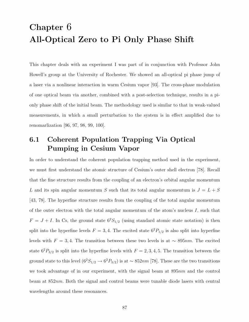
Chapter 6All-Optical Zero to Pi Only Phase Shift

This chapter deals with an experiment I was part of in conjunction with Professor John

Howell’s group at the University of Rochester. We showed an all-optical pi phase jump of

a laser via a nonlinear interaction in warm Cesium vapor [93]. The cross-phase modulation

of one optical beam via another, combined with a post-selection technique, results in a pi-

only phase shift of the initial beam. The methodology used is similar to that in weak-valued

measurements, in which a small perturbation to the system is in effect amplified due to

renomarlization [96, 97, 98, 99, 100].

6.1 Coherent Population Trapping Via Optical

Pumping in Cesium Vapor

In order to understand the coherent population trapping method used in the experiment,

we must first understand the atomic structure of Cesium’s outer shell electron [78]. Recall

that the fine structure results from the coupling of an electron’s orbital angular momentum

L and its spin angular momentum S such that its total angular momentum is J = L + S

[43, 78]. The hyperfine structure results from the coupling of the total angular momentum

of the outer electron with the total angular momentum of the atom’s nucleus I, such that

F = J + I. In Cs, the ground state 62S1/2 (using standard atomic state notation) is then

split into the hyperfine levels F = 3, 4. The excited state 62P1/2 is also split into hyperfine

levels with F = 3, 4. The transition between these two levels is at ∼ 895nm. The excited

state 62P3/2 is split into the hyperfine levels with F = 2, 3, 4, 5. The transition between the

ground state to this level (62S1/2 → 62P3/2) is at ∼ 852nm [78]. These are the two transitions

we took advantage of in our experiment, with the signal beam at 895nm and the control

beam at 852nm. Both the signal and control beams were tunable diode lasers with central

wavelengths around these resonances.

87

In our experiment, we set up an atomic dark state via coherent population trapping by

pumping the atomic system with a nearly vertically polarized signal beam at 895nm [43, 78].

Vertically polarized light may be written in the circular polarization basis as:

|V 〉 =|σ+〉 − |σ−〉√

2i. (6.1)

Thus, when we are optically pumping the Cs vapor with vertically polarized light, the right-

hand circular polarization will pump the system into a coherent superposition of the de-

generate ground state Zeeman sublevels, as discussed more in depth in the next section

[78, 79, 80, 81, 82]. This results in the system having its electrons trapped in the ground

state due to the allowed and not allowed transitions. This is then a dark state in which the

atoms are now transparent to light at 895nm, due to the coherent population trapping. An

energy level diagram showing this is seen in Figure 6.1. This dark state due to coherent pop-

FIGURE 6.1: Diagram showing CPT in Cs vapor pumped by vertically polarized light. σ+

and σ− are the left and right-hand polarization components, respectively.

ulation trapping resulting from the two circular polarization components of the signal beam

is the starting point for our experiment. The system is setup in this way, then perturbed via

methods described in the following section.

88

6.2 Optical Faraday Rotation and the Pi-Only Phase

Shift

An atomic system such as Cesium may have its degenerate Zeeman sublevels split via different

methods [43, 74, 75, 78]. A static external magnetic field applied to the system will split the

hyperfine levels into 2F + 1 Zeeman sublevels, denoted ml. An additional method that may

be used to split these hyperfine sublevels is an electric field. A laser will induce the AC Stark

effect, which is the electric field analogue to the Zeeman splitting from a magnetic field [43, 74,

75, 78]. The sublevels will be preferentially shifted (split) depending on the polarization of the

applied field. Left-hand polarized light will preferentially shift the sublevels with ∆ml = +1,

whereas right-hand polarized light preferentially shifts the sublevels with ∆ml = −1.

When circularly polarized light interacts with a system containing these nondegenerate

Zeeman sublevels, the selection rule ∆ml = ±1 applies [78]. As mentioned, left-hand circu-

larly polarized light, |σ+〉, pumps the atomic population into the transitions with ∆ml = +1,

whereas right-hand circularly polarized light, |σ−〉, cycles the transitions with ∆ml = −1.

This preferential shift of atomic state populations results in a change in index of refraction

between left and right-hand circularly polarized light. Thus, linearly polarized light such

as in equation 6.1, passing through this system will obtain a polarization rotation due to

the different indices of refraction the circularly polarized components see, due to the pref-

erential shift in nondegenerate Zeeman sublevels induced by the other, circularly polarized

beam. This rotation and resulting phase shift of one optical beam via another is known as

an optical Faraday rotation [74].

The general idea behind our experiment was to set up a dark state between the degenerate

Zeeman sublevels in Cs vapor with one nearly vertically polarized laser. These levels are split

with a small applied magnetic field. Then, another beam is overlapped in the Cs cell with

the first beam. This additional beam then has its polarization varied from completely left-

handed to completely right-handed, resulting in various polarization rotations in the first

beam, thus imparting a phase change in it. Then, by applying a post-selection similar to a

89

FIGURE 6.2: Diagram of the D1 and D2 lines in Cesium, with the signal and control beamstuned to them, respectively.

weak-valued measurement, we obtain a complete pi-phase shift of the initial beam due to the

second applied beam, though at the cost of the initial beam’s intensity. Figure 6.2 shows the

fine and hyperfine structure of Cs in our experiment. The signal beam is tuned slightly to

the red of the D1 line transition at 895nm. The control beam probes the D2 line transition

at 852nm.

In order to see the pi-only cross-phase modulation phase shift, we start by taking the input

state of the signal beam to be nearly vertically polarized:

|ψ〉1 =eiδ|σ+〉 − e−iδ|σ−〉√

2i. (6.2)

Here, δ is a measure of how far from purely vertically polarized the signal beam input is. The

beam then acquires a phase shift inside the Cs cell via the interaction with the atomic vapor

and the control beam, as previously described. The phase shift is denoted as φ, resulting in

the state:

|ψ〉2 =ei(δ+φ)|σ+〉 − e−i(δ+φ)|σ−〉√

2i. (6.3)

Writing |σ+〉 and |σ−〉, the left and right-hand circularly polarized light components respec-

tively, in the linearly polarized basis, we acquire the state:

|ψ〉2 =ei(δ+φ) − e−i(δ+φ)

2i|H〉+

ei(δ+φ) + e−i(δ+φ)

2|V 〉 = sin (δ + φ)|H〉+ cos (δ + φ)|V 〉. (6.4)

90

After leaving the Cs cell, this state is then incident on a polarizer that is very close to

orthogonal with respect to the nearly vertically polarized input state |ψ〉1. This acts as a

post-selection on the state |ψ〉2 state, selecting out the horizontal component only. Formally,

this acts as the operation of applying |H〉〈H|ψ2〉. Due to the fact that 〈H|V 〉 = 0, we are

left with the state:

|ψ〉3 = sin (δ + φ)|H〉, (6.5)

with a probability amplitude of P = sin2 (δ + φ), corresponding to the probability of a

photon emerging from the system in this state. Renormalizing the state such that:

|C|2〈ψ|ψ〉2 = 1, (6.6)

we obtain a normalization constant of C = | sin (δ + φ)|, resulting in the normalized final

output state:

|ψ〉f =sin (δ + φ)

| sin (δ + φ)||H〉. (6.7)

Thus, the output state contains coefficients of ±1 only, with no other values allowed. Hence,

any photon that makes it through the post-selection process is horizontally polarized, and

contains a complete pi-only phase shift. Now that we are armed with the physical basis for

the process resulting in the pi-only phase shift, we may discuss the experimental setup and

procedures.

6.3 Experimental Setup

The major components of the experiment described here are two lasers, a Cesium vapor cell,

two crossed polarizers, and a Mach-Zehnder interferometer. A diagram of the experimental

setup is shown in Figure 6.3. The signal beam, at 895nm, is set to nearly vertical polarization

by use of a polarizer, then sent into a Mach-Zehnder interferometer by first splitting the beam

at a 50:50 beam splitter. One arm contains a Cesium vapor cell heated to 70C. The cell is

surrounded by a solenoid in order to cancel any residual magnetic fields that may be present.

91

The other arm contains a piezo-actuated mirror in order to induce a phase shift relative to

the two arms, allowing for interference fringes to be formed when recombining the two arms

of the interferometer on another beam splitter, and looking at the balanced output signal

from the two paths. A half-wave plate is also present in this arm in order to rotate the

polarization of the signal beam to be horizontal in this path, thus allowing for the beams in

the two paths to interfere with one another.

After passing through the Cs vapor cell, the signal beam passes through another polarizer.

This is set to be almost completely orthogonal to the first polarizer, allowing only horizontally

polarized light to pass through. A control laser at 852nm is used as the phase-shift inducing

beam. This beam is first passed through an acousto-optic modulator in order to pulse it. This

allowed us to see the effect of the control beam on the system by having it alternate from

being present and turned off. It was then passed through a quarter-wave plate in order to

control its degree of circular polarization. This beam is then also input on the initial beam

splitter and passed through the Cs cell, overlapping spatially with the signal beam. This

induces the slight polarization rotation in the signal beam, as discussed in previous sections.

Filters are placed in both arms of the interferometer in order to remove the control beam

before the final beam splitter.

The intensity at the photodetectors corresponds to:

I = I0|ψf ± ψc|2, (6.8)

where ψf is the state in the free space path of the interferometer and ψc is the state of

the beam in the Cesium cell path. The total intensity is reduced by a factor of P resulting

from the post-selection process. However, the light that does pass through the post-selection

polarizer is completely out of phase with the initial input beam (it obtains only a pi-phase

shift). Thus, we can monitor the complete constructive and destructive interference resulting

from the pi-only phase shift by sweeping the phase of the free space beam with the piezo-

actuated mirror. We see that the above equation will correspond to a change from complete

92

constructive to complete destructive interference (and vice versa) when measuring the dif-

ference photocurrents at the output modes due to the fact that the coefficients of the states

may only take on values of ±1.

FIGURE 6.3: Detailed diagram of the actual experimental setup. Aom is an acousto-opticalmodulator, pbs is a polarizing beam splitter, 50:50 is a balanced beam splitter, pol is apolarizer, and λ/2 and λ/4 are half and quarter-wave plates, respectively.

The general experimental procedure is as follows. First we aligned the interferometer and

balanced photodetector without the Cs cell in the setup. We then aligned and focused the

signal and control beams such that they overlapped throughout the length of the Cs cell.

Then, we went off resonance with the signal beam (in order to allow it to pass through

the Cs cell) and changed its polarization via wave plates to be nearly vertical before the

Cs cell. The polarizer after the Cs cell was then set to be nearly orthogonal to the first

polarizer, in order to minimize the transmitted signal from it. We then changed the laser

frequency to correspond to the 895nm D1 line resonance of Cs. At this point, some signal

beam was still transmitted through the cell due to the presence of residual magnetic fields.

We then changed the magnetic field due to the solenoid surrounding the cell to cancel out

93

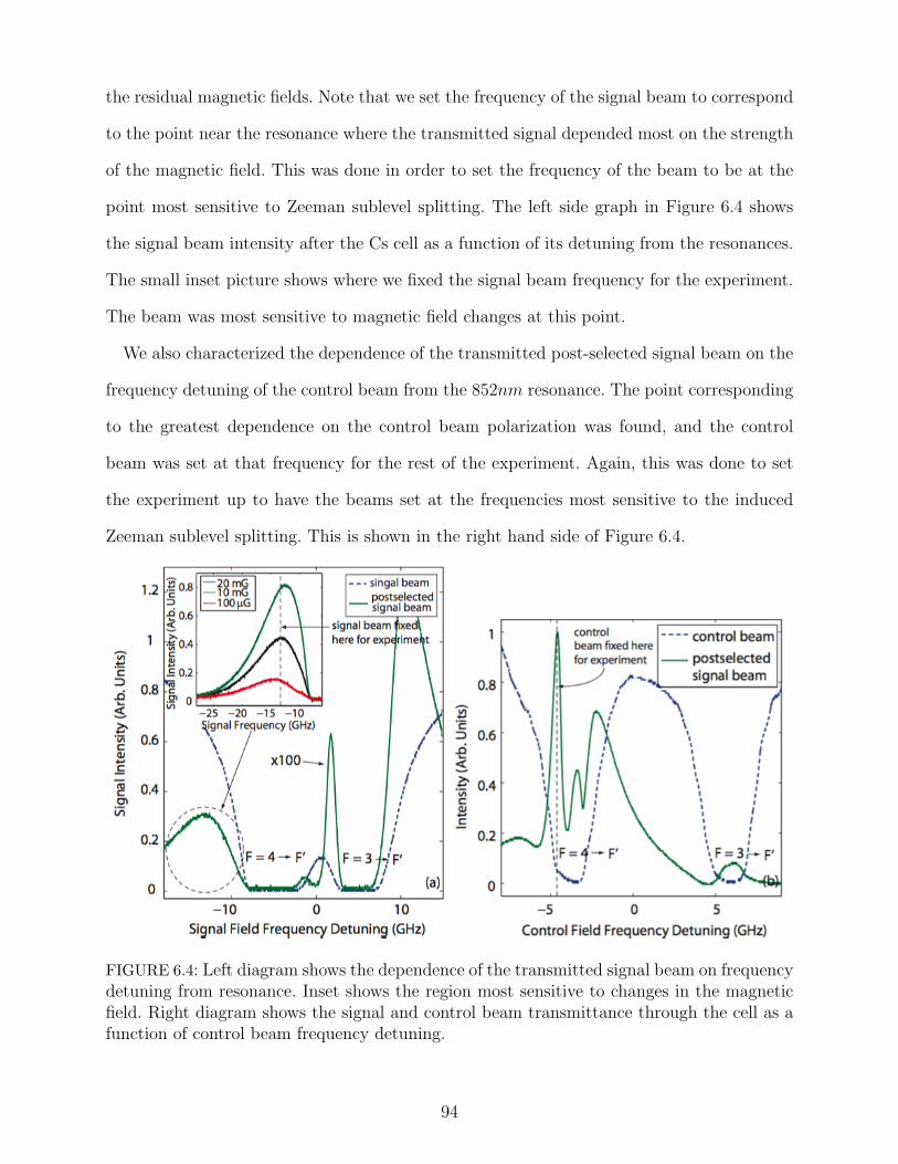
the residual magnetic fields. Note that we set the frequency of the signal beam to correspond

to the point near the resonance where the transmitted signal depended most on the strength

of the magnetic field. This was done in order to set the frequency of the beam to be at the

point most sensitive to Zeeman sublevel splitting. The left side graph in Figure 6.4 shows

the signal beam intensity after the Cs cell as a function of its detuning from the resonances.

The small inset picture shows where we fixed the signal beam frequency for the experiment.

The beam was most sensitive to magnetic field changes at this point.

We also characterized the dependence of the transmitted post-selected signal beam on the

frequency detuning of the control beam from the 852nm resonance. The point corresponding

to the greatest dependence on the control beam polarization was found, and the control

beam was set at that frequency for the rest of the experiment. Again, this was done to set

the experiment up to have the beams set at the frequencies most sensitive to the induced

Zeeman sublevel splitting. This is shown in the right hand side of Figure 6.4.

FIGURE 6.4: Left diagram shows the dependence of the transmitted signal beam on frequencydetuning from resonance. Inset shows the region most sensitive to changes in the magneticfield. Right diagram shows the signal and control beam transmittance through the cell as afunction of control beam frequency detuning.

94

6.4 Results

The experiment was then run by varying the polarization of the control beam from |σ+〉 to

|σ−〉. The balanced photodetector signal was recorded, in which we were able to very clearly

see a phase shift of pi only. As the polarization of the control beam was changed, the signal

beam’s amplitude decreased, until the point where it crosses a phase singularity resulting

from the post-selection polarizer, at which point it crosses over to a phase shift of pi. The

experiment was repeated for various control beam powers, from 660µW to 15µW . As seen in

Figure 6.5, a pi-only phase shift is very clearly demonstrated for every control beam power.

This shows that the resulting pi-only phase shift is independent of the control beam power,

hinting toward the possibility of a single-photon induced pi-only phase shift [101, 102].

FIGURE 6.5: Pi-only phase shift of the signal beam for various control beam powers. As thequarter wave plate in the control beam’s path was changed, the transmitted signal beam’sintensity lowered, then crossed over a phase singularity resulting in a complete pi-only phaseshift.

A typical example of the signal output we would see when looking at the oscilloscope

measuring the post-selected signal beam is shown in Figure 6.6. We see that when the

95

FIGURE 6.6: Pi-phase shift of the signal beam resulting from the presence of the controlbeam. The control beam is pulsed with the acousto-optic modulator so that we can see thepost-selected signal with and without the presence of the control. When the control beam ison, the phase of the signal is shifted by 180.

control beam is turned on, the phase of the post-selected signal beam is 180 shifted relative

to when the control beam is turned off. The on and off sections of the oscilloscope figure are

simply the times when the control beam pulse is present in the cell and overlapping with the

signal beam, and when a pulse is not present, respectively. Varying the polarization of the

control beam would result in the amplitude in the central portion of the figure decreasing.

A simple, yet extremely powerful graph showing the fact that the the signal beam obtains

only a pi-phase shift, and no other values is seen in Figure 6.7. This shows that while we

varied the control beam’s quarter wave plate, the phase of the post-selected signal beam

stayed constant until it reached the singularity, then immediately crossed over and obtained

a pi-phase shift. We made more measurements around the phase singularity in order to more

precisely show that the phase does not vary any between zero and pi.

This experiment shows an all-optical pi-only phase shift of one beam due to the presence

of another beam in a Cesium vapor cell. The control beam imparts a small phase shift on the

signal beam due to an optical Faraday rotation. Then, due to post-selection by way of nearly

orthogonal polarizers, the signal beam at the output obtains a pi-phase shift. The intensity

of the signal beam is reduced due to the post-selection, but the resulting phase shift is always

96

only pi. Additionally, we showed that this effect is independent of the intensity of the control

beam.

FIGURE 6.7: Pi-phase shift of the signal beam resulting from the optical Faraday rotationinduced by the control beam. The transmitted signal phase is shown for various quarter waveplate settings corresponding to different polarizations of the control beam.

97

Chapter 7Conclusions

The fields of quantum and nonlinear optics have given rise to many physical phenomena that

allow for improvements beyond limitations set by classical physics. One such improvement

specific quantum states allow for are creating interference patterns smaller than allowed by

the Rayleigh diffraction limit. This has applications primarily in imaging, where we may use

light at a longer wavelength to produce ever smaller patterns. Quantum states of light also

allow for phase measurements with much greater precision than allowed by the shot-noise

limit, allowing for improved sensitivity in interferometric measurements. Maximally path-

entangled states such as N00N states in fact reach the Heisenberg limit of ∆φ = 1/N , rather

than the shot-noise limit of ∆φ = 1/√n. Additionally, a variety of quantum states may be

used to create completely secure keys for use in cryptography. Various schemes utilize single

photons and nonorthogonal bases, while others make use of entanglement and time-energy

correlations created by various nonlinear optical phenomena.

We have seen various methods for creating squeezed and quantum states of light. One of

these methods is by the interaction of light with a crystal exhibiting a nonzero second-order

nonlinear susceptibility χ(2). When one of these nonlinear crystals is pumped with a laser and

unseeded in its signal and idler modes, spontaneous parametric down conversion occurs. This

results in perfect photon number correlations in these two output modes, as well as spatial

and temporal correlations between them. These correlations may be exploited to allow for

sub-Rayleigh imaging, sub-shot-noise limit phase estimation, and quantum key distribution.

Stimulated parametric down conversion results when a nonlinear crystal is seeded in one

or both of its signal and idler input modes. This process results in an increased rate of

down conversion relative to the spontaneous process. When a quantum state is input into

the signal and/or idler modes, the state is amplified. Photon number entangled light input

98

to these modes will be amplified in number, and may be exploited to create higher N N00N

states with relatively high efficiency compared to other linear optical schemes. The output

may also be used for quantum key distribution based on time-energy entanglement. I have

also shown a scheme I created that will convert N00N states into heralded MM’ states via

two optical parametric amplifiers and the use of number-resolving detectors. These states

are more robust to losses in interferometry than N00N states, while still able to beat the

shot-noise limit. Additionally, the stimulated parametric down conversion process may be

used to measure the absolute radiance of the source input to one of the crystal’s signal or

idler modes, by measuring the photon counts at the other mode’s output.

Another nonlinear process that may be used to create nonclassical states is via the in-

teraction of light with alkali vapor. Various effects may occur, such as four-wave mixing,

coherent population trapping, electromagnetically induced transparency, and optical Fara-

day rotations. Four-wave mixing is a χ(3) process, and involves four photons rather than three

as in the parametric down conversion case. The output probe and conjugate beams exhibit

joint quadrature squeezing due to photon number correlations resulting from the process.

This process is also multi-spatial mode, which allows for various imaging setups. When the

process is seeded with an image on the probe beam, entangled images are produced due to

the photon number correlations between the output probe and conjugate beams, as well as

their multi-spatial mode structure. This in turn allows for the transfer of entangled images

to a number of different beams by way of multiple four-wave mixing interactions, though the

degree of entanglement will decrease due to added noise. Additionally, nonlocal double slit

interference may be seen due again to the multi-spatial mode structure and photon number

correlations.

There are a number of analogies that may be drawn between the parametric down con-

version and four-wave mixing processes. This may be seen immediately upon examination

of their ideal interaction Hamiltonians. Both result in strong photon number correlations

between their output modes. They are also both multi-spatial mode, allowing for image

99

transfer and amplification. When seeded with non-vacuum inputs, both processes become

stimulated allowing for increased gains and amplification or cloning of states and images.

Another interesting effect that occurs in alkali vapor via an interaction with coherent light

is coherent population trapping. Quantum interference between probability amplitudes of

various atomic levels may result in the vapor becoming transparent to light at wavelengths

which it would normally absorb. When a signal beam in a vapor cell sets the system up in this

state, this effect may be exploited to induce a pi-only phase shift by the presence of another

light beam overlapping the signal inside the cell. The pi-only phase shift then results from

post-selection of specific output states, though at the cost of lowering the signal amplitude.

This effect was shown to be independent of the phase-shift inducing beam’s power, thus

hinting toward the possibility of a single photon induced pi-phase shift of an optical beam.

All of the effects discussed in this dissertation involve interactions between photons and

materials whose optical properties change resulting from interactions with the light. These

processes result in various effects such as creation of quantum and squeezed states of light,

quantum state and image cloning, image transfer and exploitation of entanglement, and

pi-only phase shifts.

100

References

[1] Boyd R. Nonlinear Optics. Academic Press; 2003.

[2] Gerry C, Knight P. Introductory Quantum Optics. Cambridge University Press; 2005.

[3] Drummond P, Ficek Z. Quantum Squeezing. Springer; 2004.

[4] Boto A, Kok P, Abrams D, Braunstein S, Williams C, Dowling J. Quantum Interfer-ometric Optical Lithography: Exploiting Entanglement to Beat the Diffraction Limit.Phys. Rev. Lett. 2000; 85:2733.

[5] Kleinman, D. Theory of Optical Parametric Noise. Phys. Review. 1968; 174:1027.

[6] Ali-Khan I, Howell J. Experimental demonstration of high two-photon time-energy en-tanglement. Phys. Rev. A. 2006; 73:031801.

[7] Tittel W, Zbinden H, Gisin N. Quantum Cryptography Using Entangled Photons inEnergy-Time Bell States. Phys. Rev. Lett. 2000; 84:4737.

[8] Ali-Khan I, Broadbent C, Howell J. Large-Alphabet Quantum Key Distribution UsingEnergy-Time Entangled Bipartite States. Phys. Rev. Lett. 2007; 98:060503.

[9] Levenson J, Bencheikh K, Lovering D, Vidakovic P, Simonneau C. Quantum noise in op-tical parametric amplification: a means to achieve noiseless optical functions. QuantumSemiclass. Opt. 1997; 9:221.

[10] Yuen H. Generation, Detection, and Application of High-Intensity Photon-Number-Eigenstate Fields. Phys. Rev. Lett. 1986; 56:2176.

[11] Jennewein T, Simon C, Weihs G, Weinfurter H, Zeilinger A. Quantum Cryptographywith Entangled Photons. Phys. Rev. Lett. 2000; 84:4729.

[12] Agarwal G, Chan K, Boyd R, Cable H, Dowling J. Quantum states of light producedby a high-gain optical parametric amplifier for use in quantum lithography. J. Opt. Soc.Am. B. 2007; 24:270.

[13] Grangier P, Slusher R, Yurke B, LaPorta A. Squeezed-light-enhanced polarization in-terferometer. Phys. Rev. Lett. 1987; 59:2153.

[14] Yuen H. Two-photon coherent states of the radiation field. Phys. Rev. A. 1976; 13:2226.

[15] Caves C. Quantum-mechanical noise in an interferometer. Phys. Rev. D. 1981; 23:1693.

[16] Aytur O, Kumar P. Pulsed twin beams of light. Phys. Rev. Lett. 1990; 65:1551.

[17] Heidmann A, Horowicz R, Reynaud S, Giacobino E, Fabre C, Camy G. Observation ofQuantum Noise Reduction on Twin Laser Beams. Phys. Rev. Lett. 1987; 59:2555.

[18] Levenson J, Abram I, Rivera T, Fayolle P, Garreau J, Grangier P. Quantum opticalcloning amplifier. Phys. Rev. Lett. 1993; 70:267.

101

[19] Slusher R, Grangier P, LaPorta A, Yurke B, Potasek M. Pulsed Squeezed Light. Phys.Rev. Lett. 1987; 59:2566.

[20] Levenson J, Abram I, Rivera T, Grangier P. Reduction of quantum noise in opticalparametric amplification. J. Opt. Soc. Am. B. 1993; 10:2233.

[21] Einstein A, Podolsky B, Rosen N. Can Quantum-Mechanical Description of PhysicalReality Be Considered Complete? Phys. Review. 1935; 47:777.

[22] Dowling J. Quantum optical metrology - the lowdown on high-N00N states. Cont. Phys.2008; 49:125.

[23] Holland M, Burnett K. Interferometric detection of optical phase shifts at the Heisenberglimit. Phys. Rev. Lett. 1993; 71:1355.

[24] Kapale K, Didomenico L, Lee H, Dowling J. Quantum Interferometric Sensors. 2005;2:225.

[25] Pezze L, Smerzi A. Mach-Zehnder Interferometry at the Heisenberg Limit with coherentand squeezed-vacuum light. Arxiv:quant-ph/0705.4631. 2007.

[26] Rubin M. Transverse correlation in optical spontaneous parametric down-conversion.Phys. Rev. A. 1996; 54:5349.

[27] Joobeur A, Saleh B, Larchuk T, Teich M. Coherence properties of entangled light beamsgenerated by parametric down-conversion: Theory and experiment. Phys. Rev. A. 1996;53:4360.

[28] Harris S, Oshman M, Byer R. Observation of Tunable Optical Parametric Flourescence.Phys. Rev. Lett. 1967; 18:732.

[29] Nagata T, Okamoto R, O’Brien J, Sasaki K, Takeuchi S. Beating the Standard QuantumLimit with Four-Entangled Photons. Science. 2007; 316:726.

[30] Walther P, Pan J, Aspelmeyer M, Ursin R, Gasparoni S, Zeilinger A. De Broglie wave-length of a non-local four-photon state. Nature. 2004; 429:158.

[31] Kwiat P, Vareka W, Hong C, Nathel H, Chiao R. Correlated two-photon interference ina dual-beam Michelson interferometer. Phys. Rev. A. 1990; 41:2910.

[32] Lamas-Linares A, Simon C, Howell J, Bouwmeester D. Experimental Quantum Cloningof Single Photons. Science. 2002; 296:712.

[33] Simon C, Weihs G, Zeilinger A. Optimal Quantum Cloning via Stimulated Emission.Phys. Rev. Lett. 2000; 84:2993.

[34] Kolkiran A, Agarwal G. Quantum interferometry using coherent beam stimulated para-metric down-conversion. Opt. Express. 2008; 16:6479.

[35] Caminati M, De Martini F, Perris R, Sciarrino F, Secondi V. Entanglement, EPR cor-relations and mesoscopic quantum superposition by the high-gain quantum injectedparametric amplification. arXiv:quant-ph/0609100. 2006.

102

[36] Glasser R, Cable H, Dowling J, De Martini F, Sciarrino F, Vitelli C. Entanglement-seeded, dual, optical parametric amplification: Applications to quantum imaging andmetrology. Phys. Rev. A. 2008; 78:012339.

[37] Ribeiro P, Caetano D, Almeida M, Huguenin J, Coutinho dos Santos B, Khoury A.Observation of Image Transfer and Phase Conjugation in Stimulated Down-Conversion.Phys. Rev. Lett. 2001; 87:133602.

[38] Ribeiro P, Padua S, Monken C. Image and coherence transfer in the stimulated down-conversion process. Phys. Rev. A. 1999; 60:5074.

[39] Migdall, A. Absolute Quantum Efficiency Measurements Using Correlated Photons:Toward a Measurement Protocol. IEEE Transactions on Instrumentation and Measure-ment. 2001; 50:478.

[40] Migdall A, Datla R, Sergienko A, Orszak J, Shih Y. Measuring absolute infrared spec-tral radiance with correlated visible photons: technique verification and measurementuncertainty. Applied Opt. 1998; 37:3455.

[41] Pack M, Camacho R, Howell J. Transients of the electromagnetically-induced-transparency-enhanced refractive Kerr nonlinearity: Theory. 2006; 74:013812.

[42] Li Yong-qing, Xiao M. Electromagnetically induced transparency in a three-level Λ-typesystem in rubidium atoms. Phys. Rev. A. 1995; 51:R2703.

[43] Budker D, Gawlik W, Kimball D, Rochester S, Yashchuk V, Weis A. Resonant nonlinearmagneto-optical effects in atoms. Rev. of Mod. Phys. 2002; 74:1153.

[44] Harris S. Electromagnetically Induced Transparency. Physics Today. July 1997; 36.

[45] Slusher R, Yurke B, Grangier P, LaPorta A, Walls D, Reid M. Squeezed-light generationby four-wave mixing near an atomic resonance. J. Opt. Soc. Am. B. 1987; 4:1453.

[46] Boyer V, Marino A, Pooser R, Lett P. Entangled Images from Four-Wave Mixing. Sci-ence. 2008; 321:544.

[47] McCormick C, Boyer V, Arimondo E, Lett P. Strong relative intensity squeezing byfour-wave mixing in rubidium vapor. Opt. Lett. 2007; 32:178.

[48] McCormick C, Marino A, Boyer V, Lett P. Strong low-frequency quantum correlationsfrom a four-wave-mixing amplifier. Phys. Rev. A. 2008; 78:043816.

[49] Wu L, Xiao M, Kimble H. Squeezed states of light from an optical parametric oscillator.J. Opt. Soc. Am. B. 1987; 4:1465.

[50] Stothard D, Ebrahimzadeh M, Dunn M. Low-pump-threshold continuous-wave singlyresonant optical parametric oscillator. 1998; 23:1895.

[51] Brosnan S, Byer R. Optical parametric oscillator threshold and linewidth studies. IEEEJ. Quant. Elec. 1979; 15:415.

103

[52] Drummond P, Reid M. Correlations in nondegenerate parametric oscillation. II. Belowthreshold results. Phys. Rev. A. 1990; 41:3930.

[53] Reid M, Drummond P. Quantum Correlations of Phase in Nondegenerate ParametricOscillation. Phys. Rev. Lett. 1988; 60:2731.

[54] Pooser R, Pfister O. Particle-number scaling of the phase sensitivity in realistic Bayesiantwin-mode Heisenberg-limited interferometry. Phys. Rev. A. 2004; 69:043616.

[55] Shor P. Polynomial-Time Algorithms for Prime Factorization and Discrete Logarithmson a Quantum Computer. J. Sci. Statist. Comput. 1997; 26:1484.

[56] Bennett C, Brassard G. Quantum Cryptography: Public key distribution and coin toss-ing. Proc. IEEE Int. Conf. on Computers, Systems and Signal Processing. 1984; 175.

[57] Bennett C. Quantum cryptography using any two nonorthogonal states. Phys. Rev.Lett. 1992; 68:3121.

[58] Hong C, Ou Z, Mandel L. Measurement of subpicosecond time intervals between twophotons by interference. Phys. Rev. Lett. 1987; 59:2044.

[59] Lee H, Kok P, Cerf N, Dowling P. Linear optics and projective measurements alonesuffice to create large-photon-number path entanglement. Phys. Rev. A. 2002; 65:030101.

[60] Cable H, Dowling J. Efficient Generation of Large Number-Path Entanglement UsingOnly Linear Optics and Feed-Forward. Phys. Rev. Lett. 2007; 99:163604.

[61] Durkin G, Dowling J. Local and Global Distinguishability in Quantum Interferometry.Phys. Rev. Lett. 2007; 99:070801.

[62] Gilbert G, Hamrick M, Weinstein Y. Practical quantum interferometry using photonicN00N states. Proc. SPIE. 2007; 6573:65730K

[63] Rubin M, Kaushik S. Loss-induced limits to phase measurement precision with maxi-mally entangled states. Phys. Rev. A. 2007; 75:053805.

[64] Huver S, Wildfeuer C, Dowling J. Entangled Fock states for robust quantum opticalmetrology, imaging, and sensing. Phys. Rev. A. 2008; 78:063828.

[65] Bouwmeester D, Ekert A, Zeilinger A. The Physics of Quantum Information. Springer.2000.

[66] Bell J. On the problem of hidden variables in quantum mechanics. Rev. Mod. Phys.1966; 38:447.

[67] Clauser J, Horne M, Shimony A, Holt R. Proposed Experiment to Test Local Hidden-Variable Theories. Phys. Rev. Lett. 1969; 23:880.

[68] Franson J. Bell inequality for position and time. Phys. Rev. Lett. 1989; 62:2205.

[69] Franken P, Hill A, Peters C, Weinreich G. Generation of Optical Harmonics. Phys. Rev.Lett. 1961; 7:118.

104

[70] Howell J. Franson Interference: Space-like separated method for determining time-timecorrelations of entangled photons:http://www.pas.rochester.edu/ howell/mysite2/Tutorials/Franson%20Interference.pdf

[71] Kim Y, Kulik S, Shih Y. High-intensity pulsed source of space-time and polarizationdouble-entangled photon pairs. Phys. Rev. A. 2000; 62:011802.

[72] Aspelmeyer M, Bohm H, Gyatso T, Jennewein T, Kaltenbaek R, Lindenthal M, Molina-Terriza G, Poppe A, Resch K, Taraba M, Ursin R, Walther P, Zeilinger A. Long-DistanceFree-Space Distribution of Quantum Entanglement. Science. 2006; 301:621.

[73] Sergienko A, Shih Y, Rubin M. Experimental evaluation of a two-photon wave packetin type-II parametric downconversion. J. Opt. Soc. Am. B. 1995; 12:859.

[74] Cho D, Choi J, Kim J, Park Q-Han. Optically induced Faraday effect using three-levelatoms. Phys. Rev. A. 2005; 72:012821.

[75] Park C, Noh H, Lee C, Cho D. Measurement of the Zeeman-like ac Stark shift. Phys.Rev. A. 2001; 63:032512.

[76] Harris S, Hau L. Nonlinear Optics at Low Light Levels. Phys. Rev. Lett. 1999; 82:4611.

[77] Kang H, Zhu Y. Observation of Large Kerr Nonlinearity at Low Light Intensities. Phys.Rev. Lett. 2003; 91:093601.

[78] Steck D. Cesium D Line Data. Los Alamos National Laboratory, Theoretical Division.2003.

[79] Lu B, Burkett W, Xiao M. Nondegenerate four-wave mixing in a double-Λ system underthe influence of coherent population trapping. Opt. Lett. 1998; 23:804.

[80] Stahler M, Wynands R, Knappe S, Kitching J, Hollberg L, Taichenachev A, YudinV. Coherent population trapping resonances in thermal 85Rb vapor: D1 versus D2 lineexcitation. Opt. Lett. 2002. 27:1472.

[81] Ling H, Li Y, Xiao M. Coherent population trapping and electromagnetically inducedtransparency in multi-Zeeman-sublevel atoms. Phys. Rev. A. 1996; 53:1014.

[82] Fleischhauer M, Imamoglu A, Marangos J. Electromagnetically induced transparency:Optics in coherent media. Rev. Mod. Phys. 2005; 77:633.

[83] De Martini F. Amplification of Quantum Entanglement. Phys. Rev. Lett. 1998; 81:2842.

[84] Agarwal G, Tara K. Nonclassical properties of states generated by the excitations on acoherent state. Phys. Rev. A. 1991; 43:492.

[85] Li Y, Jing H, Zhan M. Simultaneous creations of discrete-variable entangled state andsingle-photon-added coherent state. Arxiv:quant-ph/0610137. 2006.

[86] Ono T, Hofmann H. Quantum enhancement of N-photon phase sensitivity by interfero-metric addition of down-converted photon pairs to weak coherent light. Arxiv:quant/ph-0708.2809. 2008.

105

[87] Sciarrino F, Vitelli C, De Martini F, Glasser R, Cable H, Dowling J. Experimental sub-Rayleigh resolution by an unseeded high-gain optical parametric amplifier for quantumlithography. Phys. Rev. A. 2008; 77:012324.

[88] Rosenberg D, Lita A, Miller A, Nam S. Noise-free high-efficiency photon-number-resolving detectors. Phys. Rev. A. 2005; 71:061803.

[89] Lee H, Yurtsever U, Kok P, Hockney G, Adami C, Braunstein S, Dowling J. TowardsPhotostatistics from Number Resolving Photodetectors. J. Mod. Opt. 2004; 51:1517.

[90] Byer R, Harris S. Power and Bandwidth of Spontaneous Parametric Emission. Phys.Review. 1968; 168:1064.

[91] Ling A, Lamas-Linares A, Kurtsiefer C. Absolute emission rates of Spontaneous Para-metric Down Conversion into single transverse Gaussian modes. Phys. Rev. A. 2008;77:043834.

[92] Boeuf N, Branning D, Chaperot I, Dauler E, Guerin S, Jaeger G, Muller A, MigdallA. Calculating Characteristics of Non-collinear Phase-matching in Uniaxial and BiaxialCrystals. http://physics.nist.gov/Divisions/Div844/facilities/cprad/cprad.html 1999

[93] Camacho R, Dixon B, Glasser R, Jordan A, Howell J. Realization of an All-Optical Zeroto π Cross-Phase Modulation Jump. Phys. Rev. Lett. 2009; 102:013902.

[94] Monken C, Ribeiro P, Padua S. Transfer of angular spectrum and image formation inspontaneous parametric down-conversion. Phys. Rev. A. 1998; 57:3123.

[95] Fonseca E, Ribeiro P, Padua S, Monken C. Quantum interference by a nonlocal doubleslit. Phys. Rev. A. 1999; 60:1530.

[96] Ritchie N, Story J, Hulet R. Realization of a measurement of a ”weak value”. Phys.Rev. Lett. 1991; 66:1107.

[97] Pryde G, O’brien J, White A, Ralph T, Wiseman H. Measurement of Quantum WeakValues of Photon Polarization. Phys. Rev. Lett. 2005; 94:220405.

[98] Hosten O, Kwiat P. Observation of the Spin Hall Effect of Light via Weak Measurements.Science. 2008; 319:787.

[99] Aharonov Y, Albert D, Vaidman L. How the result of a measurement of a componentof the spin of a spin-1/2 particle can turn out to be 100. Phys. Rev. Lett. 1988; 60:1351.

[100] Duck I, Stevenson P, Sudarshan E. The sense in which a ”weak measurement” of aspin-1/2 particle’s spin component yields a value 100. Phys. Rev. D. 1989; 40:2112.

[101] Harris S, Yamamoto Y. Photon Switching by Quantum Interference. Phys. Rev. Lett.1998; 81:3611.

[102] Yan M, Rickey E, Zhu Y. Observation of absorptive photon switching by quantuminterference. Phys. Rev. A. 2001; 64:041801.

106

[103] O’Sullivan-Hale M, Ali-Khan I, Boyd R, Howell J. Pixel Entanglement: Experimen-tal Realization of Optically Entangled d=3 and d=6 Qudits. Phys. Rev. Lett. 2005;94:220501.

107

Vita

Ryan T. Glasser was born in May 1982, in Redlands, California, to Thomas D. Glasser

and Susan C. Glasser. He earned a bachelor of science degree in physics with a minor in

mathematics at the University of California, Los Angeles, in May 2005. In August of 2005

he came to Louisiana State University to pursue a Doctor of Philosophy degree in physics.

He is specializing in quantum optics, under the advisement of Prof. Jonathan Dowling. He

is currently a doctoral candidate expecting to graduate in May 2009.

108