Correlated Errors in the Parameters Estimation of the ARFIMA Model: A Simulated Study

Communications in Statistics—Simulation and Computation®, 35: 789–802, 2006Copyright © Taylor & Francis Group, LLCISSN: 0361-0918 print/1532-4141 onlineDOI: 10.1080/03610910600716928

Time Series Analysis

Correlated Errors in the Parameters Estimation of theARFIMAModel: A Simulated Study

M. R. SENA Jr.1, V. A. REISEN2, AND S. R. C. LOPES3

1Department of Statistics, Federal University of Pernambuco,Recife, Brazil2Department of Statistics, Federal University of Espírito Santo,Vitória, Brazil3Department of Statistics, Federal University of Rio Grande do Sul, PortoAlegre, Brazil

Processes with correlated errors have been widely used in economic timeseries. The fractionally integrated autoregressive moving-average processes—ARFIMA(p� d� q)—(Hosking, 1981) have been explored to model stationary and nonstationary time series with long-memory property. This work uses the MonteCarlo simulation method to evaluate the performance of some parametric andsemiparametric estimators for long and short-memory parameters of the ARFIMAmodel with conditional heteroskedastic (ARFIMA-GARCH model). The comparisonis based on the empirical bias and the mean squared error of each estimator.

Keywords Fractional differencing; Long memory and GARCH models.

Mathematics Subject Classification 62M10; 62M15.

1. Introduction

Recently, the analysis of time series with long memory has been widely arguedin the literature. Since the ARFIMA�p� d� q� model was introduced by Grangerand Joyeux (1980) and Hosking (1981), many estimation methods of the memoryparameter d have been proposed and some corrections of the estimators havebeen suggested to improve their statistical properties. Amongst the usually so-called parametric approaches we mention the works of Fox and Taqqu (1986),Dahlhaus (1989), and Sowell (1992) which are estimation methods based on themaximum likelihood theory. Among the semiparametric approaches we cite theworks of Geweke and Porter-Hudak (1983), Robinson (1994, 1995), Reisen (1994),

Received February 27, 2004; Accepted November 23, 2005Address correspondence to V. A. Reisen, Department of Statistics, Federal University

of Espírito Santo, Vitória, Brazil; E-mail: [email protected]

789

790 Sena et al.

and Lobato and Robinson (1996). Bootstrap estimation procedures for d has beenthe focus of Franco and Reisen (2004) and references therein. The estimationmethods for memory parameters of seasonal fractionally ARMA models have beendiscussed and investigated empirically by Reisen et al. (2006a,b). In this article, theauthors have also presented the invertibility and casual parameters conditions of themodel.

The main goal of this article is to evaluate, through a simulation study, thebias and the robustness of six estimation methods for the fractional differencingparameter d in ARFIMA processes with heteroskedastic errors. This research topichas recently received considerable attention in a variety of studies in time series andeconometric areas. Ling and Li (1997), Henry (2001a,b), and Jensen (2004) haveprovided a good survey of the literature. The ARFIMA-GARCH model and itsparameter estimators have been considered in Ling and Li (1997). The authors havederived some sufficient conditions for stationarity and ergodicity, and an algorithmfor approximate maximum likelihood estimation has been also presented. Henry(2001a) has focused his research on the estimation of the memory parameter ofa time series with long-memory conditional heteroskedasticity (ARFIMA-GARCHmodel) by using the average periodogram estimator suggested in Robinson (1994).In this context, Henry (2001a) has shown that the average periodogram estimatorremains consistent. This semiparametric memory parameter estimation method isalso considered here. The choice of the optimal bandwidth for some semiparametricestimation methods, under a general form of the errors such as GARCH errors, hasbeen the focus of Henry (2001b). The author has derived optimal bandwidths andhas shown asymptotically that the estimators considered in his work are not affectedby conditional heteroskedasticity property of the innovations.

Jensen (2004) has given contributions based on Bayesian approach toestimate the memory parameter in long-memory stochastic volatility processes. Anapplication of the useful ARFIMA-GARCH model in inflation data has been thefocus of Baillie et al. (1996).

The results reported here increase our understanding of the finite sampleproperties of some fractional memory parameter estimators of the ARFIMA modelwith heteroscedastic errors. The plan of this article is as follows. Section 2 outlinesthe use of ARFIMA model with GARCH errors. Section 3 presents a summary onthe estimation methods for the parameter d. Section 4 discusses the set-up of theMonte Carlo experiment and the results. Some conclusions are drawn in Sec. 5.

2. The ARFIMA Model with GARCH Errors

Let �Xt�t∈Z be a time series presented in a set of information available at an instantt − 1. If �t−1 is a set of evaluated available information at an instant t − 1, we canrepresent �Xt�t∈Z by the form

Xt = g��t−1� b�+ �t� (2.1)

where g�· � ·� is a function, b is a vector of the parameters to be estimated, and�t is a random perturbation. Equation (2.1) is sufficiently general and it has beenstudied and shaped by many authors. The most common specification for it is the

Parameters Estimation of the ARFIMA Model 791

autoregressive AR�p� model and the moving average MA�q� model that can be mixedto have the ARMA�p� q� model, described hereof by

�����Xt − � = ����t� t ∈ Z� (2.2)

where � is the backward operator such that �kXt = Xt−k, ���� = 1−∑pj=1 �j�

j ,��� = 1−∑q

i=1 �i�i, p and q are positive integers, is the mean of the process,

and ��t�t∈Z is a white noise process with zero mean and constant variance 2� .

���� and ��� are polynomials with all roots outside the unit circle and share nocommon factors.

Studies in economic time series have shown that the dependent variable—returns in the interest rates, for instance—presents significant autocorrelation, evenfor lags largely separated in time. Time series with this behavior is said to havelong-memory property and it may be modeled by the ARFIMA�p� d� q� modeldescribed as

�����1−��d�Xt − � = ����t� t ∈ Z� (2.3)

where d is a real number.When d ∈ �−0�5� 0�5�, the ARFIMA�p� d� q� process is said to be invertible and

stationary and its spectral density function fX�·� ·� is given by

fX�w� �� = fU �w� ��

[2 sin

(w

2

)]−2d

� w ∈ �−�� ��� (2.4)

where fU �w� �� is the spectral density function of an ARMA�p� q� process and �and � are the unknown parameter vectors of the ARMA and ARFIMA models,respectively. Hosking (1981), Beran (1994), and Reisen (1994) have described theARFIMA models with more details. Engle (1982) has defined the process conditionalautoregressive heteroskedastic (ARCH) when �t is of the form

�t = zt t� (2.5)

where zt is an independent and identically distributed process with E�zt� = 0 andVar�zt� = 1 and t, varying in time, is a function of the set �t−1. By definition,the variables �t are not autocorrelated, for any t ∈ Z, but its conditional variancedepends on time, opposing to what is assumed for the usual least squares estimationmethod. The ARCH�s� model or its generalization GARCH�s� r� model can besummarized here, through the form of the innovation variance for the time t,according to Eq. (2.1) and with the assumption that �t��t−1 ∼ � �0� 2

t �, where

2t = �0 +

s∑i=1

�i�2t−i +

r∑j=1

�j 2t−j� (2.6)

where s and r are positive integers, �i ≥ 0, for i ∈ �0� 1� � � � � s�, and �j ≥ 0, forj ∈ �1� 2� � � � � r�.

Bollerslev (1986) has shown that a GARCH process is stationary if ��1�+��1� < 1, where ��1� = ∑s

i=1 �i and ��1� = ∑rj=1 �j , whenever E��t� = 0, Var��t� =

�0/�1− ��1�− ��1�� and the innovation process is not autocorrelated. We remark

792 Sena et al.

here that if one excludes the last sum in Eq. (2.6), one has the simplest model, anARCH�s� model.

The combination of models in expressions (2.3), (2.5), and (2.6) yields to theARFIMA �p� d� q�-GARCH�r� s� model. Under the parameter conditions for ����,���, ��1�, and ��1�, as previously described, the ARFIMA�p� d� q�-GARCH�r� s�process is stationary and invertible if −0�5 ≤ d ≤ 0�5, see Theorem 2.3 in Lingand Li (1997). The authors have also demonstrated the condition for ergodicityand derived the existence of higher-order moments. To estimate the parameters,an algorithm for approximate maximum likelihood (ML) estimation has been alsopresented by the authors.

The autocorrelation function of ARFIMA�p� d� q�-GARCH�r� s� modelbehaves asymptotically with the similar form of the stationary ARFIMA model.This means that the dependency between observations decays hyperbolically as afunction of d. Based on this autocorrelation behavior, we are here interested instudying the estimation of the parameter d for some parameter order specificationsof the ARFIMA�p� d� q�-GARCH�r� s� model. This empirical study will providean evidence whether the memory estimators are robust or not under conditionalheteroskedasticity. It is worth noting that all estimation methods focused here havebeen previously implemented to the estimation of the stationary and non stationaryARFIMA processes see, for instance, Lopes et al. (2004) and Reisen et al. (2001a)for an overview.

3. Estimation of d

We consider six estimators for the parameter d and provide a summary of eachmethod below. The first four approaches are based on the linear regression methodbuilt from Eq. (2.4) and are considered semiparametric methods. The averagedperiodogram estimator also belongs to the semiparametric class. The remaining twoestimators are the parametric methods proposed by Fox and Taqqu (1986) andSowell (1992).

The first estimator, denoted hereafter by d̂Per , has been proposed by Gewekeand Porter-Hudak (1983). They use the periodogram function I�·� as an estimatorfor the spectral density function, presented in Eq. (2.4). The number of regressorsused in the regression equation is a function of the sample size n and it is denotedhere by g�n� = n�, for 0 < � < 1.

The second estimator, denoted by d̂Per S , has been proposed by Reisen (1994).The author has made a modification in the regression equation, substituting theperiodogram function by its smoothing version based on the Parzen lag window. Inthis estimator the function g�n� = n�, for 0 < � < 1, is also chosen to represent thenumber of regressors in the regression equation. The truncation point in the Parzenlag window is denoted by m = n�, for 0 < � < 1. The appropriate choices of � and� values had been investigated by Geweke and Porter-Hudak (1983) and Reisen(1994), respectively, among several other authors.

The third estimator, denoted hereafter by d̂Lob, has been considered byRobinson (1994) and Lobato and Robinson (1996). It is a weighted average of thelogarithm of the periodogram function. This estimator is based on a number offrequencies � and on a constant q ∈ �0�0� 1�0�. Lobato and Robinson (1996) havepresented a Monte Carlo simulated experiment to investigate the sensitivity on thechoice of � and q values.

Parameters Estimation of the ARFIMA Model 793

The fourth estimator, denoted by d̂Rob, has been introduced by Robinson(1995). This method is also a modified version of the Geweke and Porter-Hudak’sestimator. This estimator regresses ln�I�wj�� on ln�2 sin�wj/2��

2, for j = l� l+1� � � � � g�n�, where l is the smallest truncated point that tends to infinity smootherthan g�n�. Robinson (1995) has developed some asymptotic results for d̂Rob, whend ∈ �0�0� 0�5�, and has showed that this estimator is asymptotically less efficient thanthe Gaussian maximum likelihood estimator and in this situation the efficiency isconsidered to be zero. The number of regressors g�n� can take different forms andits appropriate choice has been studied by several authors, such as Robinson (1995),Hurvich et al. (1998), and Hurvich and Deo (1999), to name just a few.

The fifth estimator, hereafter denoted by d̂Fox, is a parametric procedure thathas been considered by Fox and Taqqu (1986), based on the work of Whittle (1953).The estimates are obtained by minimizing the finite and discrete form given by

�n��� =12n

n−1∑j=1

{ln fX�wj� ��+

I�wj�

fX�wj� ��

}� (3.1)

where � denotes the vector of unknown parameters and fX�w� �� is the spectraldensity function (see Dahlhaus, 1989; Fox and Taqqu, 1986).

The ML estimator (see Sowell, 1992) is the sixth method focused here. Assumingthat the process �Xt� is Gaussian, the log-likelihood function may be expressed as

�n��� = −12log det T�fX�w� ���−

12X′T�fX�w� ���

−1X� (3.2)

where � is the parameter vector and T is the variance–covariance matrix of theprocess �Xt�t∈Z with �j� k�th element given by

Tjk�fX�w� ��� =12�

∫ �

−�fX�w� �� exp�iwjk�dw�

see for example Beran (1994, Sec. 5.3). The ML estimates are obtained bymaximizing (3.2), that is, �̂ = argmax�n���. Following the estimator notationsadopted here the ML fractional estimator is denoted by d̂ML.

Fractional integration has been applied in models like GARCH, including theFIGARCH model by Chung (1999), the FIEGARCH model by Baillie et al. (1994),and the FIAPARCH model by Tse (1998). All of them have in common somevariations in the estimation process through the maximization of the likelihoodfunction. The comparison among parameter estimation procedures have been widelystudied and they are sources of research for several authors. However, it is notour main goal. This article focuses on the robustness of the estimators for thefractional parameter d, in view of violating the normality assumption for theinnovation process and also in the study of how they are affected by the existenceof heteroskedastic errors.

4. Monte Carlo Simulation Study

In order to investigate the robustness of the estimators described previously,in the context of ARFIMA models with GARCH errors, a number of Monte

794 Sena et al.

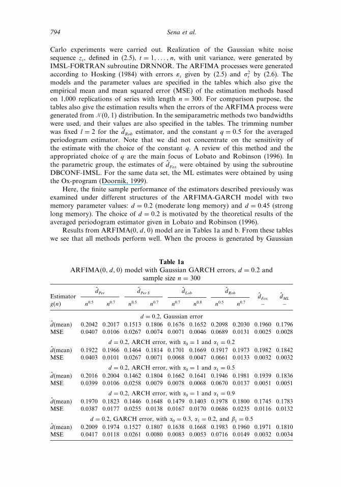
Carlo experiments were carried out. Realization of the Gaussian white noisesequence zt, defined in (2.5), t = 1� � � � � n, with unit variance, were generated byIMSL-FORTRAN subroutine DRNNOR. The ARFIMA processes were generatedaccording to Hosking (1984) with errors �t given by (2.5) and 2

t by (2.6). Themodels and the parameter values are specified in the tables which also give theempirical mean and mean squared error (MSE) of the estimation methods basedon 1,000 replications of series with length n = 300. For comparison purpose, thetables also give the estimation results when the errors of the ARFIMA process weregenerated from � �0� 1� distribution. In the semiparametric methods two bandwidthswere used, and their values are also specified in the tables. The trimming numberwas fixed l = 2 for the d̂Rob estimator, and the constant q = 0�5 for the averagedperiodogram estimator. Note that we did not concentrate on the sensitivity ofthe estimate with the choice of the constant q. A review of this method and theappropriated choice of q are the main focus of Lobato and Robinson (1996). Inthe parametric group, the estimates of d̂Fox were obtained by using the subroutineDBCONF-IMSL. For the same data set, the ML estimates were obtained by usingthe Ox-program (Doornik, 1999).

Here, the finite sample performance of the estimators described previously wasexamined under different structures of the ARFIMA-GARCH model with twomemory parameter values: d = 0�2 (moderate long memory) and d = 0�45 (stronglong memory). The choice of d = 0�2 is motivated by the theoretical results of theaveraged periodogram estimator given in Lobato and Robinson (1996).

Results from ARFIMA(0� d� 0� model are in Tables 1a and b. From these tableswe see that all methods perform well. When the process is generated by Gaussian

Table 1aARFIMA�0� d� 0� model with Gaussian GARCH errors, d = 0�2 and

sample size n = 300

d̂Per d̂Per S d̂Lob d̂RobEstimator d̂Fox d̂ML

g�n� n0�5 n0�7 n0�5 n0�7 n0�7 n0�8 n0�5 n0�7 – –

d = 0�2, Gaussian errord̂(mean) 0�2042 0�2017 0�1513 0�1806 0�1676 0�1652 0�2098 0�2030 0�1960 0�1796MSE 0�0407 0�0106 0�0267 0�0074 0�0071 0�0046 0�0689 0�0131 0�0025 0�0028

d = 0�2, ARCH error, with �0 = 1 and �1 = 0�2d̂(mean) 0�1922 0�1966 0�1464 0�1814 0�1701 0�1669 0�1917 0�1973 0�1982 0�1842MSE 0�0403 0�0101 0�0267 0�0071 0�0068 0�0047 0�0661 0�0133 0�0032 0�0032

d = 0�2, ARCH error, with �0 = 1 and �1 = 0�5d̂(mean) 0�2016 0�2004 0�1462 0�1804 0�1662 0�1641 0�1946 0�1981 0�1939 0�1836MSE 0�0399 0�0106 0�0258 0�0079 0�0078 0�0068 0�0670 0�0137 0�0051 0�0051

d = 0�2, ARCH error, with �0 = 1 and �1 = 0�9d̂(mean) 0�1970 0�1823 0�1446 0�1648 0�1479 0�1403 0�1978 0�1800 0�1745 0�1783MSE 0�0387 0�0177 0�0255 0�0138 0�0167 0�0170 0�0686 0�0235 0�0116 0�0132

d = 0�2, GARCH error, with �0 = 0�3, �1 = 0�2, and �1 = 0�5d̂(mean) 0�2009 0�1974 0�1527 0�1807 0�1638 0�1668 0�1983 0�1960 0�1971 0�1810MSE 0�0417 0�0118 0�0261 0�0080 0�0083 0�0053 0�0716 0�0149 0�0032 0�0034

Parameters Estimation of the ARFIMA Model 795

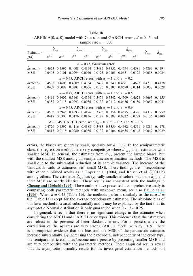
Table 1bARFIMA�0� d� 0� model with Gaussian and GARCH errors, d = 0�45 and

sample size n = 300

d̂Per d̂Per S d̂Lob d̂RobEstimator d̂Fox d̂ML

g�n� n0�5 n0�7 n0�5 n0�7 n0�7 n0�8 n0�5 n0�7 – –

d = 0�45, Gaussian errord̂(mean) 0�4623 0�4592 0�4008 0�4394 0�3487 0�3552 0�4594 0�4581 0�4869 0�4194MSE 0�0405 0�0101 0�0294 0�0070 0�0125 0�0105 0�0631 0�0128 0�0038 0�0024

d = 0�45, ARCH error, with �0 = 1 and �1 = 0�2d̂(mean) 0�4595 0�4608 0�4009 0�4384 0�3479 0�3540 0�4661 0�4627 0�4770 0�4178MSE 0�0409 0�0092 0�0281 0�0066 0�0126 0�0107 0�0670 0�0114 0�0038 0�0028

d = 0�45, ARCH error, with �0 = 1 and �1 = 0�5d̂(mean) 0�4491 0�4605 0�3961 0�4394 0�3474 0�3542 0�4509 0�4628 0�4663 0�4155MSE 0�0387 0�0115 0�0293 0�0086 0�0132 0�0112 0�0636 0�0150 0�0057 0�0041

d = 0�45, ARCH error, with �0 = 1 and �1 = 0�9d̂(mean) 0�4502 0�3945 0�4393 0�4196 0�3325 0�3354 0�4575 0�4396 0�4377 0�3959MSE 0�0418 0�0300 0�0176 0�0136 0�0189 0�0188 0�0722 0�0229 0�0136 0�0100

d = 0�45, GARCH error, with �0 = 0�3, �1 = 0�2, and �1 = 0�5d̂(mean) 0�4729 0�4592 0�4116 0�4388 0�3483 0�3559 0�4662 0�4551 0�4884 0�4178MSE 0�0413 0�0118 0�0280 0�0086 0�0132 0�0106 0�0654 0�0148 0�0049 0�0029

errors, the biases are generally small, specially for d = 0�2. In the semiparametricclass, the regression methods are very competitive where d̂Per S is an estimator withsmaller MSE. In general, the estimates from d̂Lob present the largest biases, butwith the smallest MSE among all semiparametric estimation methods. The MSE issmall due to the substantial reduction of its sample variance. The increase of thebandwidth leads to estimates with small MSE. These findings are in accordancewith other published works as in Lopes et al. (2004) and Reisen et al. (2001a,b)among others. The estimator d̂Fox has typically smaller absolute bias than d̂ML andtheir MSE are nearly identical. These results are consistent with the findings inCheung and Diebold (1994). These authors have presented a comprehensive analysiscomparing both parametric methods with unknown mean, see also Baillie et al.(1996). When d = 0�45 (Table 1b), the methods perform similarly to the case d =0�2 (Table 1a) except for the average periodogram estimator. The absolute bias ofthis later method increased substantially and it may be explained by the fact that itsasymptotic Normal distribution is only guarantied when 0 < d < 0�25.

In general, it seems that there is no significant change in the estimates whenconsidering the ARCH and GARCH error types. This evidences that the estimatorsare robust in the presence of heteroskedastic errors. For a process where thecorrelation of the squares are very strong (ARCH model with �1 = 0�9), thereis an empirical evidence that the bias and the MSE of the parametric estimatesincrease substantially. By increasing the bandwidth, independently of the error type,the semiparametric estimates become more precise by presenting smaller MSE andare very competitive with the parametric methods. These empirical results revealthat the asymptotic normality results for the investigated estimation methods still

796 Sena et al.

hold for heteroskedastic errors. Similar findings using the average periodogram andparametric estimators are, respectively, in Henry (2001a) and Baillie et al. (1996).

Reisen et al. (2001a) have studied the robustness of these estimators when theerrors come from a non normal distribution. Their empirical investigation haveevidenced that the estimators have no influence with the violation of normalityassumption, and have called the attention of the good performance of theparametric estimator d̂Fox under correct model specification.

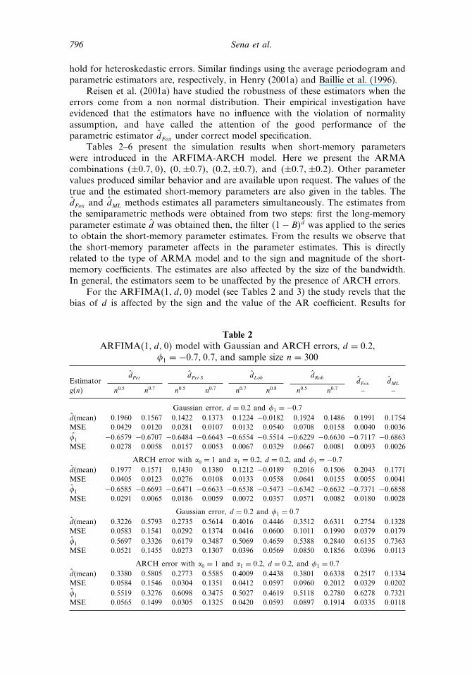
Tables 2–6 present the simulation results when short-memory parameterswere introduced in the ARFIMA-ARCH model. Here we present the ARMAcombinations �±0�7� 0�, �0�±0�7�, �0�2�±0�7�, and �±0�7�±0�2�. Other parametervalues produced similar behavior and are available upon request. The values of thetrue and the estimated short-memory parameters are also given in the tables. Thed̂Fox and d̂ML methods estimates all parameters simultaneously. The estimates fromthe semiparametric methods were obtained from two steps: first the long-memoryparameter estimate d̂ was obtained then, the filter �1− B�d̂ was applied to the seriesto obtain the short-memory parameter estimates. From the results we observe thatthe short-memory parameter affects in the parameter estimates. This is directlyrelated to the type of ARMA model and to the sign and magnitude of the short-memory coefficients. The estimates are also affected by the size of the bandwidth.In general, the estimators seem to be unaffected by the presence of ARCH errors.

For the ARFIMA�1� d� 0� model (see Tables 2 and 3) the study revels that thebias of d is affected by the sign and the value of the AR coefficient. Results for

Table 2ARFIMA�1� d� 0� model with Gaussian and ARCH errors, d = 0�2,

�1 = −0�7� 0�7, and sample size n = 300

d̂Per d̂Per S d̂Lob d̂RobEstimator d̂Fox d̂ML

g�n� n0�5 n0�7 n0�5 n0�7 n0�7 n0�8 n0�5 n0�7 – –

Gaussian error, d = 0�2 and �1 = −0�7d̂(mean) 0�1960 0�1567 0�1422 0�1373 0�1224 −0�0182 0�1924 0�1486 0�1991 0�1754MSE 0�0429 0�0120 0�0281 0�0107 0�0132 0�0540 0�0708 0�0158 0�0040 0�0036�̂1 −0�6579 −0�6707 −0�6484 −0�6643 −0�6554 −0�5514 −0�6229 −0�6630 −0�7117 −0�6863MSE 0�0278 0�0058 0�0157 0�0053 0�0067 0�0329 0�0667 0�0081 0�0093 0�0026

ARCH error with �0 = 1 and �1 = 0�2, d = 0�2, and �1 = −0�7d̂(mean) 0�1977 0�1571 0�1430 0�1380 0�1212 −0�0189 0�2016 0�1506 0�2043 0�1771MSE 0�0405 0�0123 0�0276 0�0108 0�0133 0�0558 0�0641 0�0155 0�0055 0�0041�̂1 −0�6585 −0�6693 −0�6471 −0�6633 −0�6538 −0�5473 −0�6342 −0�6632 −0�7371 −0�6858MSE 0�0291 0�0065 0�0186 0�0059 0�0072 0�0357 0�0571 0�0082 0�0180 0�0028

Gaussian error, d = 0�2 and �1 = 0�7d̂(mean) 0�3226 0�5793 0�2735 0�5614 0�4016 0�4446 0�3512 0�6311 0�2754 0�1328MSE 0�0583 0�1541 0�0292 0�1374 0�0416 0�0600 0�1011 0�1990 0�0379 0�0179�̂1 0�5697 0�3326 0�6179 0�3487 0�5069 0�4659 0�5388 0�2840 0�6135 0�7363MSE 0�0521 0�1455 0�0273 0�1307 0�0396 0�0569 0�0850 0�1856 0�0396 0�0113

ARCH error with �0 = 1 and �1 = 0�2, d = 0�2, and �1 = 0�7d̂(mean) 0�3380 0�5805 0�2773 0�5585 0�4009 0�4438 0�3801 0�6338 0�2517 0�1334MSE 0�0584 0�1546 0�0304 0�1351 0�0412 0�0597 0�0960 0�2012 0�0329 0�0202�̂1 0�5519 0�3276 0�6098 0�3475 0�5027 0�4619 0�5118 0�2780 0�6278 0�7321MSE 0�0565 0�1499 0�0305 0�1325 0�0420 0�0593 0�0897 0�1914 0�0335 0�0118

Parameters Estimation of the ARFIMA Model 797

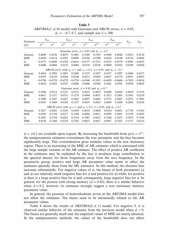
Table 3ARFIMA�1� d� 0� model with Gaussian and ARCH errors, d = 0�45,

�1 = −0�7� 0�7, and sample size n = 300

d̂Per d̂Per S d̂Lob d̂RobEstimator d̂Fox d̂ML

g�n� n0�5 n0�7 n0�5 n0�7 n0�7 n0�8 n0�5 n0�7 – –

Gaussian error, d = 0�45 and �1 = −0�7d̂(mean) 0�4660 0�4156 0�4079 0�3961 0�3249 0�2593 0�4580 0�4044 0�5412 0�4114MSE 0�0428 0�0114 0�0292 0�0098 0�0186 0�0398 0�0626 0�0148 0�0126 0�0034�̂1 −0�6531 −0�6688 −0�6354 −0�6616 −0�6177 −0�5513 −0�6225 −0�6579 −0�8905 −0�6823MSE 0�0440 0�0068 0�0332 0�0064 0�0118 0�0336 0�0680 0�0102 0�0549 0�0024

ARCH error, with �0 = 1 and �1 = 0�2, d = 0�45, and �1 = −0�7d̂(mean) 0�4416 0�3993 0�3891 0�3840 0�3157 0�2437 0�4357 0�3897 0�4480 0�4137MSE 0�0392 0�0129 0�0284 0�0140 0�0212 0�0456 0�0627 0�0170 0�0051 0�0035�̂1 −0�6700 −0�6758 −0�6578 −0�6754 −0�6366 −0�5851 −0�6459 −0�6686 −0�7639 −0�6816MSE 0�0624 0�0505 0�0525 0�0496 0�0496 0�0588 0�1061 0�0593 0�0708 0�0029

Gaussian error, d = 0�45 and �1 = 0�7d̂(mean) 0�5806 0�8313 0�5233 0�8122 0�4622 0�4822 0�6098 0�8824 0�8659 0�3159MSE 0�0611 0�1557 0�0331 0�1379 0�0004 0�0011 0�1013 0�2003 0�1965 0�0250�̂1 0�5680 0�3287 0�6267 0�3465 0�6997 0�6802 0�5375 0�2807 0�2972 0�7891MSE 0�0567 0�1489 0�0320 0�1327 0�0019 0�0023 0�0889 0�1890 0�2062 0�0120

ARCH error with �0 = 1 and �1 = 0�2, d = 0�45, and �1 = 0�7d̂(mean) 0�5837 0�8285 0�5245 0�8109 0�4618 0�4820 0�6250 0�8821 0�7750 0�3205MSE 0�0585 0�1538 0�0317 0�1369 0�0004 0�0011 0�0999 0�2001 0�1339 0�0245�̂1 0�5687 0�3354 0�6262 0�3514 0�7007 0�6812 0�5264 0�2855 0�3955 0�7850MSE 0�0556 0�1448 0�0314 0�1302 0�0023 0�0027 0�0887 0�1855 0�1557 0�0114

� = ±0�2 are available upon request. By increasing the bandwidth from g�n� = n0�5,the semiparametric estimates overestimate the true parameter and the bias becomessignificantly large. This overestimation gives estimate values in the non stationaryregion. There is an increasing of the MSE of AR estimates which is associated withthe large sample variance of the AR estimate. The effect of positive AR coefficientin the estimates may be explained by the fact it produces large contribution tothe spectral density for those frequencies away from the zero frequency. In theparametric group, positive and large AR parameter value seems to affect theestimates specially those from the ML estimator. In this method, the absolute biasincreases substantially. For negative values of �, the biases of both parameters (dand �) are relatively small (negative bias for d and positive for �) while, for positive� there is a large positive bias for d and, consequently, large negative bias for �. Ingeneral, for the process with strong memory (d = 0�45), there is a similar behaviorwhen d = 0�2, however, its estimates strongly suggest a non stationary memoryparameter value.

In general, the presence of heteroskedastic errors in the ARFIMA model doesnot affect the estimates. The biases seem to be intrinsically related to the ARparameter values.

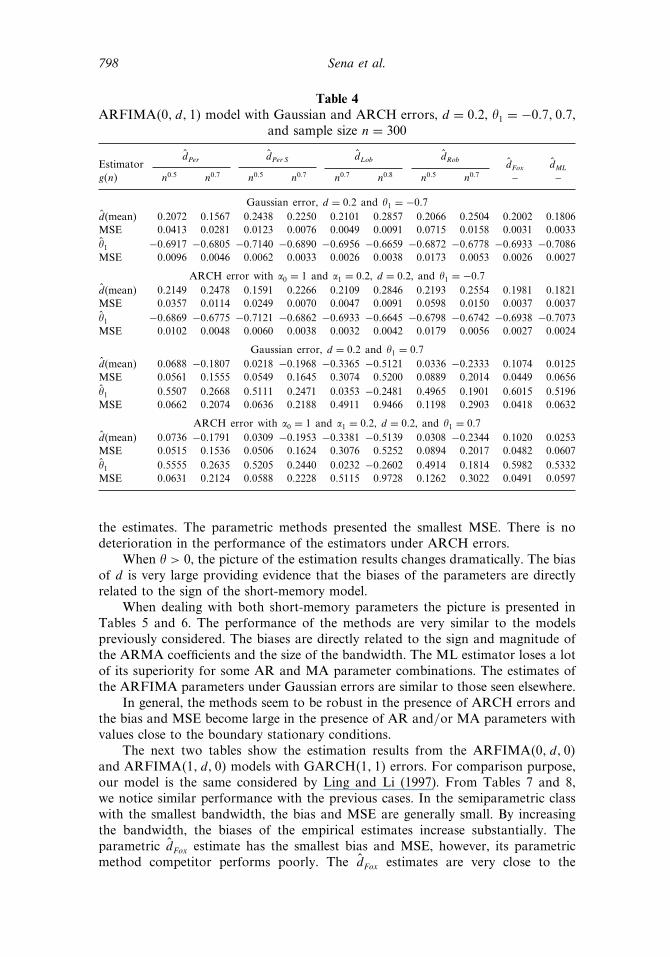
Table 4 shows the results of ARFIMA�0� d� 1� model. For negative �, it isobserved similar behavior of the estimates from the previous model when � < 0.The biases are generally small and, the empirical values of MSE are nearly identical.In the semiparametric methods, the values of the bandwidth does not affect

798 Sena et al.

Table 4ARFIMA�0� d� 1� model with Gaussian and ARCH errors, d = 0�2, �1 = −0�7� 0�7,

and sample size n = 300

d̂Per d̂Per S d̂Lob d̂RobEstimator d̂Fox d̂ML

g�n� n0�5 n0�7 n0�5 n0�7 n0�7 n0�8 n0�5 n0�7 – –

Gaussian error, d = 0�2 and �1 = −0�7d̂(mean) 0�2072 0�1567 0�2438 0�2250 0�2101 0�2857 0�2066 0�2504 0�2002 0�1806MSE 0�0413 0�0281 0�0123 0�0076 0�0049 0�0091 0�0715 0�0158 0�0031 0�0033�̂1 −0�6917 −0�6805 −0�7140 −0�6890 −0�6956 −0�6659 −0�6872 −0�6778 −0�6933 −0�7086MSE 0�0096 0�0046 0�0062 0�0033 0�0026 0�0038 0�0173 0�0053 0�0026 0�0027

ARCH error with �0 = 1 and �1 = 0�2, d = 0�2, and �1 = −0�7d̂(mean) 0�2149 0�2478 0�1591 0�2266 0�2109 0�2846 0�2193 0�2554 0�1981 0�1821MSE 0�0357 0�0114 0�0249 0�0070 0�0047 0�0091 0�0598 0�0150 0�0037 0�0037�̂1 −0�6869 −0�6775 −0�7121 −0�6862 −0�6933 −0�6645 −0�6798 −0�6742 −0�6938 −0�7073MSE 0�0102 0�0048 0�0060 0�0038 0�0032 0�0042 0�0179 0�0056 0�0027 0�0024

Gaussian error, d = 0�2 and �1 = 0�7d̂(mean) 0�0688 −0�1807 0�0218 −0�1968 −0�3365 −0�5121 0�0336 −0�2333 0�1074 0�0125MSE 0�0561 0�1555 0�0549 0�1645 0�3074 0�5200 0�0889 0�2014 0�0449 0�0656�̂1 0�5507 0�2668 0�5111 0�2471 0�0353 −0�2481 0�4965 0�1901 0�6015 0�5196MSE 0�0662 0�2074 0�0636 0�2188 0�4911 0�9466 0�1198 0�2903 0�0418 0�0632

ARCH error with �0 = 1 and �1 = 0�2, d = 0�2, and �1 = 0�7d̂(mean) 0�0736 −0�1791 0�0309 −0�1953 −0�3381 −0�5139 0�0308 −0�2344 0�1020 0�0253MSE 0�0515 0�1536 0�0506 0�1624 0�3076 0�5252 0�0894 0�2017 0�0482 0�0607�̂1 0�5555 0�2635 0�5205 0�2440 0�0232 −0�2602 0�4914 0�1814 0�5982 0�5332MSE 0�0631 0�2124 0�0588 0�2228 0�5115 0�9728 0�1262 0�3022 0�0491 0�0597

the estimates. The parametric methods presented the smallest MSE. There is nodeterioration in the performance of the estimators under ARCH errors.

When � > 0, the picture of the estimation results changes dramatically. The biasof d is very large providing evidence that the biases of the parameters are directlyrelated to the sign of the short-memory model.

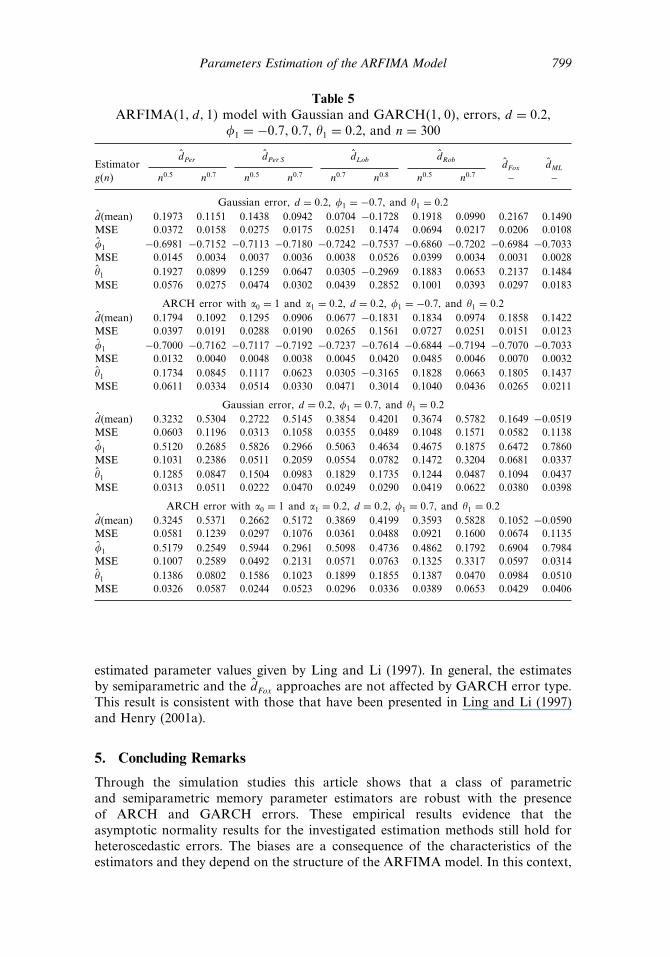
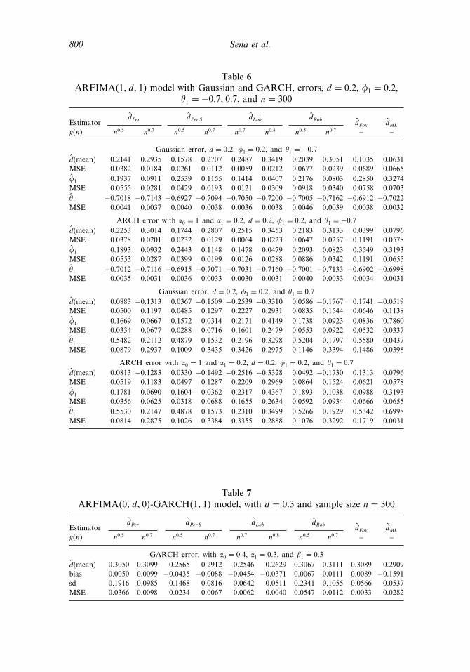
When dealing with both short-memory parameters the picture is presented inTables 5 and 6. The performance of the methods are very similar to the modelspreviously considered. The biases are directly related to the sign and magnitude ofthe ARMA coefficients and the size of the bandwidth. The ML estimator loses a lotof its superiority for some AR and MA parameter combinations. The estimates ofthe ARFIMA parameters under Gaussian errors are similar to those seen elsewhere.

In general, the methods seem to be robust in the presence of ARCH errors andthe bias and MSE become large in the presence of AR and/or MA parameters withvalues close to the boundary stationary conditions.

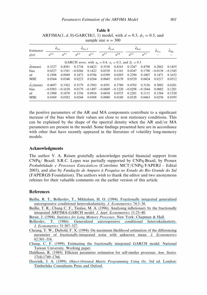
The next two tables show the estimation results from the ARFIMA�0� d� 0�and ARFIMA�1� d� 0� models with GARCH�1� 1� errors. For comparison purpose,our model is the same considered by Ling and Li (1997). From Tables 7 and 8,we notice similar performance with the previous cases. In the semiparametric classwith the smallest bandwidth, the bias and MSE are generally small. By increasingthe bandwidth, the biases of the empirical estimates increase substantially. Theparametric d̂Fox estimate has the smallest bias and MSE, however, its parametricmethod competitor performs poorly. The d̂Fox estimates are very close to the

Parameters Estimation of the ARFIMA Model 799

Table 5ARFIMA�1� d� 1� model with Gaussian and GARCH�1� 0�, errors, d = 0�2,

�1 = −0�7� 0�7, �1 = 0�2, and n = 300

d̂Per d̂Per S d̂Lob d̂RobEstimator d̂Fox d̂ML

g�n� n0�5 n0�7 n0�5 n0�7 n0�7 n0�8 n0�5 n0�7 – –

Gaussian error, d = 0�2, �1 = −0�7, and �1 = 0�2d̂(mean) 0�1973 0�1151 0�1438 0�0942 0�0704 −0�1728 0�1918 0�0990 0�2167 0�1490MSE 0�0372 0�0158 0�0275 0�0175 0�0251 0�1474 0�0694 0�0217 0�0206 0�0108�̂1 −0�6981 −0�7152 −0�7113 −0�7180 −0�7242 −0�7537 −0�6860 −0�7202 −0�6984 −0�7033MSE 0�0145 0�0034 0�0037 0�0036 0�0038 0�0526 0�0399 0�0034 0�0031 0�0028�̂1 0�1927 0�0899 0�1259 0�0647 0�0305 −0�2969 0�1883 0�0653 0�2137 0�1484MSE 0�0576 0�0275 0�0474 0�0302 0�0439 0�2852 0�1001 0�0393 0�0297 0�0183

ARCH error with �0 = 1 and �1 = 0�2, d = 0�2, �1 = −0�7, and �1 = 0�2d̂(mean) 0�1794 0�1092 0�1295 0�0906 0�0677 −0�1831 0�1834 0�0974 0�1858 0�1422MSE 0�0397 0�0191 0�0288 0�0190 0�0265 0�1561 0�0727 0�0251 0�0151 0�0123�̂1 −0�7000 −0�7162 −0�7117 −0�7192 −0�7237 −0�7614 −0�6844 −0�7194 −0�7070 −0�7033MSE 0�0132 0�0040 0�0048 0�0038 0�0045 0�0420 0�0485 0�0046 0�0070 0�0032�̂1 0�1734 0�0845 0�1117 0�0623 0�0305 −0�3165 0�1828 0�0663 0�1805 0�1437MSE 0�0611 0�0334 0�0514 0�0330 0�0471 0�3014 0�1040 0�0436 0�0265 0�0211

Gaussian error, d = 0�2, �1 = 0�7, and �1 = 0�2d̂(mean) 0�3232 0�5304 0�2722 0�5145 0�3854 0�4201 0�3674 0�5782 0�1649 −0�0519MSE 0�0603 0�1196 0�0313 0�1058 0�0355 0�0489 0�1048 0�1571 0�0582 0�1138�̂1 0�5120 0�2685 0�5826 0�2966 0�5063 0�4634 0�4675 0�1875 0�6472 0�7860MSE 0�1031 0�2386 0�0511 0�2059 0�0554 0�0782 0�1472 0�3204 0�0681 0�0337�̂1 0�1285 0�0847 0�1504 0�0983 0�1829 0�1735 0�1244 0�0487 0�1094 0�0437MSE 0�0313 0�0511 0�0222 0�0470 0�0249 0�0290 0�0419 0�0622 0�0380 0�0398

ARCH error with �0 = 1 and �1 = 0�2, d = 0�2, �1 = 0�7, and �1 = 0�2d̂(mean) 0�3245 0�5371 0�2662 0�5172 0�3869 0�4199 0�3593 0�5828 0�1052 −0�0590MSE 0�0581 0�1239 0�0297 0�1076 0�0361 0�0488 0�0921 0�1600 0�0674 0�1135�̂1 0�5179 0�2549 0�5944 0�2961 0�5098 0�4736 0�4862 0�1792 0�6904 0�7984MSE 0�1007 0�2589 0�0492 0�2131 0�0571 0�0763 0�1325 0�3317 0�0597 0�0314�̂1 0�1386 0�0802 0�1586 0�1023 0�1899 0�1855 0�1387 0�0470 0�0984 0�0510MSE 0�0326 0�0587 0�0244 0�0523 0�0296 0�0336 0�0389 0�0653 0�0429 0�0406

estimated parameter values given by Ling and Li (1997). In general, the estimatesby semiparametric and the d̂Fox approaches are not affected by GARCH error type.This result is consistent with those that have been presented in Ling and Li (1997)and Henry (2001a).

5. Concluding Remarks

Through the simulation studies this article shows that a class of parametricand semiparametric memory parameter estimators are robust with the presenceof ARCH and GARCH errors. These empirical results evidence that theasymptotic normality results for the investigated estimation methods still hold forheteroscedastic errors. The biases are a consequence of the characteristics of theestimators and they depend on the structure of the ARFIMA model. In this context,

800 Sena et al.

Table 6ARFIMA�1� d� 1� model with Gaussian and GARCH, errors, d = 0�2, �1 = 0�2,

�1 = −0�7� 0�7, and n = 300

d̂Per d̂Per S d̂Lob d̂RobEstimator d̂Fox d̂ML

g�n� n0�5 n0�7 n0�5 n0�7 n0�7 n0�8 n0�5 n0�7 – –

Gaussian error, d = 0�2, �1 = 0�2, and �1 = −0�7d̂(mean) 0�2141 0�2935 0�1578 0�2707 0�2487 0�3419 0�2039 0�3051 0�1035 0�0631MSE 0�0382 0�0184 0�0261 0�0112 0�0059 0�0212 0�0677 0�0239 0�0689 0�0665�̂1 0�1937 0�0911 0�2539 0�1155 0�1414 0�0407 0�2176 0�0803 0�2850 0�3274MSE 0�0555 0�0281 0�0429 0�0193 0�0121 0�0309 0�0918 0�0340 0�0758 0�0703�̂1 −0�7018 −0�7143 −0�6927 −0�7094 −0�7050 −0�7200 −0�7005 −0�7162 −0�6912 −0�7022MSE 0�0041 0�0037 0�0040 0�0038 0�0036 0�0038 0�0046 0�0039 0�0038 0�0032

ARCH error with �0 = 1 and �1 = 0�2, d = 0�2, �1 = 0�2, and �1 = −0�7d̂(mean) 0�2253 0�3014 0�1744 0�2807 0�2515 0�3453 0�2183 0�3133 0�0399 0�0796MSE 0�0378 0�0201 0�0232 0�0129 0�0064 0�0223 0�0647 0�0257 0�1191 0�0578�̂1 0�1893 0�0932 0�2443 0�1148 0�1478 0�0479 0�2093 0�0823 0�3549 0�3193MSE 0�0553 0�0287 0�0399 0�0199 0�0126 0�0288 0�0886 0�0342 0�1191 0�0655�̂1 −0�7012 −0�7116 −0�6915 −0�7071 −0�7031 −0�7160 −0�7001 −0�7133 −0�6902 −0�6998MSE 0�0035 0�0031 0�0036 0�0033 0�0030 0�0031 0�0040 0�0033 0�0034 0�0031

Gaussian error, d = 0�2, �1 = 0�2, and �1 = 0�7d̂(mean) 0�0883 −0�1313 0�0367 −0�1509 −0�2539 −0�3310 0�0586 −0�1767 0�1741 −0�0519MSE 0�0500 0�1197 0�0485 0�1297 0�2227 0�2931 0�0835 0�1544 0�0646 0�1138�̂1 0�1669 0�0667 0�1572 0�0314 0�2171 0�4149 0�1738 0�0923 0�0836 0�7860MSE 0�0334 0�0677 0�0288 0�0716 0�1601 0�2479 0�0553 0�0922 0�0532 0�0337�̂1 0�5482 0�2112 0�4879 0�1532 0�2196 0�3298 0�5204 0�1797 0�5580 0�0437MSE 0�0879 0�2937 0�1009 0�3435 0�3426 0�2975 0�1146 0�3394 0�1486 0�0398

ARCH error with �0 = 1 and �1 = 0�2, d = 0�2, �1 = 0�2, and �1 = 0�7d̂(mean) 0�0813 −0�1283 0�0330 −0�1492 −0�2516 −0�3328 0�0492 −0�1730 0�1313 0�0796MSE 0�0519 0�1183 0�0497 0�1287 0�2209 0�2969 0�0864 0�1524 0�0621 0�0578�̂1 0�1781 0�0690 0�1604 0�0362 0�2317 0�4367 0�1893 0�1038 0�0988 0�3193MSE 0�0356 0�0625 0�0318 0�0688 0�1655 0�2634 0�0592 0�0934 0�0666 0�0655�̂1 0�5530 0�2147 0�4878 0�1573 0�2310 0�3499 0�5266 0�1929 0�5342 0�6998MSE 0�0814 0�2875 0�1026 0�3384 0�3355 0�2888 0�1076 0�3292 0�1719 0�0031

Table 7ARFIMA�0� d� 0�-GARCH�1� 1� model, with d = 0�3 and sample size n = 300

d̂Per d̂Per S d̂Lob d̂RobEstimator d̂Fox d̂ML

g�n� n0�5 n0�7 n0�5 n0�7 n0�7 n0�8 n0�5 n0�7 – –

GARCH error, with �0 = 0�4, �1 = 0�3, and �1 = 0�3d̂(mean) 0�3050 0�3099 0�2565 0�2912 0�2546 0�2629 0�3067 0�3111 0�3089 0�2909bias 0�0050 0�0099 −0�0435 −0�0088 −0�0454 −0�0371 0�0067 0�0111 0�0089 −0�1591sd 0�1916 0�0985 0�1468 0�0816 0�0642 0�0511 0�2341 0�1055 0�0566 0�0537MSE 0�0366 0�0098 0�0234 0�0067 0�0062 0�0040 0�0547 0�0112 0�0033 0�0282

Parameters Estimation of the ARFIMA Model 801

Table 8ARFIMA�1� d� 0�-GARCH�1� 1� model, with d = 0�3, �1 = 0�5, and

sample size n = 300

d̂Per d̂Per S d̂Lob d̂RobEstimator d̂Fox d̂ML

g�n� n0�5 n0�7 n0�5 n0�7 n0�7 n0�8 n0�5 n0�7 – –

GARCH error, with �0 = 0�4, �1 = 0�3, and �1 = 0�3d̂(mean) 0�3227 0�4581 0�2734 0�4422 0�3538 0�4161 0�3247 0�4798 0�2862 0�1455bias 0�0227 0�1581 −0�0266 0�1422 0�0538 0�1161 0�0247 0�1798 −0�0138 −0�1545sd 0�1898 0�0949 0�1472 0�0786 0�0399 0�0205 0�2290 0�1007 0�1471 0�1652MSE 0�0364 0�0340 0�0223 0�0264 0�0045 0�0139 0�0529 0�0424 0�0217 0�0512

�̂1(mean) 0�4697 0�3362 0�5179 0�3503 0�4391 0�3780 0�4702 0�3156 0�5002 0�6281bias −0�0303 −0�1638 0�0179 −0�1497 −0�0609 −0�1220 −0�0298 −0�1844 0�0002 0�1281sd 0�1900 0�1070 0�1556 0�0916 0�0658 0�0555 0�2281 0�1111 0�1584 0�1520MSE 0�0369 0�0382 0�0244 0�0308 0�0080 0�0180 0�0528 0�0463 0�0250 0�0395

the positive parameters of the AR and MA components contribute to a significantincrease of the bias when their values are close to non stationary conditions. Thiscan be explained by the shape of the spectral density when the AR and/or MAparameters are present in the model. Some findings presented here are in accordancewith other that have recently appeared in the literature of volatility long-memorymodels.

Acknowledgments

The author V. A. Reisen gratefully acknowledges partial financial support fromCNPq/ Brazil. S.R.C. Lopes was partially supported by CNPq-Brazil, by PronexProbabilidade e Processos Estocásticos (Convênio MCT/CNPq/FAPERJ - Edital2003), and also by Fundação de Amparo à Pesquisa no Estado do Rio Grande do Sul(FAPERGS Foundation). The authors wish to thank the editor and two anonymousreferees for their valuable comments on the earlier version of this article.

References

Baillie, R. T., Bollerslev, T., Mikkelsen, H. O. (1994). Fractionally integrated generalizedautoregressive conditional heteroskedasticity. J. Econometrics 74:3–30.

Baillie, T. R., Chung C. F., Tieslau, M. A. (1996). Analysing inflationary by the fractionallyintegrated ARFIMA-GARCH model. J. Appl. Econometrics 11:23–40.

Beran, J. (1994). Statistics for Long Memory Processes. New York: Chapman & Hall.Bollerslev, T. (1986). Generalized autoregressive conditional heteroskedasticity.

J. Econometrics 31:307–327.Cheung, Y. W., Diebold, F. X. (1994). On maximum likelihood estimation of the differencing

parameter of fractionally-integrated noise with unknown mean. J. Econometrics62:301–316.

Chung, C. F. (1999). Estimating the fractionally integrated GARCH model. NationalTaiwan University. Working paper.

Dahlhaus, R. (1989). Efficient parameter estimation for self-similar processes. Ann. Statist.17(4):1749–1766.

Doornik, J. A. (1999). Object-Oriented Matrix Programming Using Ox. 3rd ed. London:Timberlake Consultants Press and Oxford.

802 Sena et al.

Engle, R. F. (1982). Autoregressive conditional heteroskedasticity with estimates of thevariance of United Kingdom inflation. Econometrica 50(4):987–1007.

Fox, R., Taqqu, M. S. (1986). Large-sample properties of parameter estimates for stronglydependent stationary Gaussian time series. Ann. Statist. 14(2):517–532.

Franco, G. C., Reisen, V. A. (2004). Bootstrap techniques in semiparametric estimationmethods for ARFIMA models: A comparison study. Computat. Statist. 19:243–259.

Geweke, J., Porter-Hudak, S. (1983). The estimation and application of long memory timeseries model. J. Time Ser. Anal. 4(4):221–238.

Granger, C. W. J., Joyeux, R. (1980). An introduction to long-memory time series modelsand fractional differencing. J. Time Ser. Anal. 1:15–29.

Henry, M. (2001a). Averaged periodogram spectral estimation with long-memory conditionalheteroscedasticity. J. Time Ser. Anal. 22(4):431–459.

Henry, M. (2001b). Robust automatic bandwidth for long memory. J. Time Ser. Anal.22(3):293–316.

Hosking, J. (1981). Fractional differencing. Biometrika 68(1):165–176.Hosking, J. (1984). Modelling persistence in hydrological time series using fractional

differencing. Water Resour. Res. 20(12):1898–1908.Hurvich, C. M., Deo, R. S. (1999). Plug-in selection of the number of frequencies in

regression estimates of the memory parameter of a long-memory time series. J. Time Ser.Anal. 20(3):331–341.

Hurvich, C. M., Deo, R. S., Brodsky, J. (1998). The mean squared error of Geweke andPorter-Hudak’s estimator of the memory parameter of a long memory time series. J. TimeSer. Anal. 19(1):19–46.

Jensen, J. M. (2004). Semiparametric Bayesian inference of long-memory stochastic volatilitymodels. J. Time Ser. Anal. 25(6):895–922.

Ling, S., Li, K. W. (1997). On fractionally integrated autoregressive moving-average timeseries with conditional heteroscedasticity. J. Amer. Statist. Assoc. 439:1184–1194.

Lobato, I., Robinson, P. M. (1996). Averaged periodogram estimation of long memory.J. Econometrics 73:303–324.

Lopes, S. R. C., Olbermann, B. P., Reisen, V. A. (2004). Comparison of estimation methodsin non-stationary ARFIMA process. J. Statist. Computat. Simul. 74(5):339–347.

Reisen, V. A. (1994). Estimation of the fractional difference parameter in theARIMA�p� d� q� model using the smoothed periodogram. J. Time Ser. Anal. 15(3):335–350.

Reisen, V. A., Abraham, B., Lopes, S. R. C. (2001a). Estimation of parameters in ARFIMA�p� d� q� process. Commun. Statist. B 30(4):787–803.

Reisen, V. A., Sena, Jr. M. R., Lopes, S. R. C. (2001b). Error and order misspecification inARFIMA models. The Brazil. Rev. Econometrics 21(1):62–79.

Reisen, V. A., Rodrigues, A., Palma, W. (2006a). Estimation of seasonal fractionallyintegrated processes. Computat. Statist. Data Analy. 50:568–582.

Reisen, V. A., Rodrigues, A., Palma, W. (2006b). Estimating seasonal long-memoryprocesses: a Monte Carlo study. Journal of Statistical Computation and Simulation76(4):305–316.

Robinson, P. M. (1994). Semiparametric analysis of long-memory time series. Ann. Statist.22:515–539.

Robinson, P. M. (1995). Log-periodogram regression of time series with long rangedependence. Ann. Statist. 23(3):1048–1072.

Sowell, F. (1992). Maximum likelihood estimation of stationary univariate fractionallyintegrated time series models. J. Econometrics 53:165–188.

Tse, Y. K. (1998). Conditional heteroskedasticity of the Yen-dollar exchange rate. J. Appl.Econometrics 13:49–55.

Whittle, P. (1953). Estimation and information in stationary time series. Arkiv för Matematik2:423–434.