Department of Economics and Business Economics Aarhus University Fuglesangs Allé 4 DK-8210 Aarhus V Denmark Email: [email protected] Tel: +45 8716 5515 Does the ARFIMA really shift? Davide Delle Monache, Stefano Grassi and Paolo Santucci de Magistris CREATES Research Paper 2017-16

Welcome message from author
This document is posted to help you gain knowledge. Please leave a comment to let me know what you think about it! Share it to your friends and learn new things together.
Transcript

Department of Economics and Business Economics
Aarhus University
Fuglesangs Allé 4
DK-8210 Aarhus V
Denmark
Email: [email protected]
Tel: +45 8716 5515
Does the ARFIMA really shift?
Davide Delle Monache, Stefano Grassi and
Paolo Santucci de Magistris
CREATES Research Paper 2017-16

Does the ARFIMA really shift?∗
Davide Delle Monache† Stefano Grassi ‡ Paolo Santucci de Magistris §
November 8, 2016
Abstract
Short memory models contaminated by level shifts have long-memory features sim-
ilar to those associated to processes generated under fractional integration. In this
paper, we propose a robust testing procedure, based on an encompassing parametric
specification, that allows to disentangle the level shift term from the ARFIMA com-
ponent. The estimation is carried out via a state-space methodology and it leads to a
robust estimate of the fractional integration parameter also in presence of level shifts.
The Monte Carlo simulations show that this approach produces unbiased estimates
of the fractional integration parameter when shifts in the mean, or in other slowly
varying trends, are present in the data. Once the fractional integration parameter is
estimated, the KPSS test statistic is adopted to assess if the level shift component
is statistically significant. The test has correct size and generally the highest power
compared to other existing tests for spurious long-memory. Finally, we illustrate the
usefulness of the proposed approach on the daily series of bipower variation and share
turnover and on the monthly inflation series of G7 countries.
Keywords: ARFIMA Processes, Level Shifts, State-Space methods, KPSS test.
JEL Classification: C10, C11, C22, C80.
∗We are grateful to Domenico Giannone, Liudas Giraitis, Emmanuel Guerre, Niels Haldrup, GeorgeKapetanios and David Veredas for useful comments and discussions. We would also like to thank theparticipants at the 7th Computational and Financial Econometrics conference (London, 2013), the 3rdLong Memory Symposium (Aarhus, 2013), the 3rd IAAE conference (Milan, 2016) and at the seminars heldat the Erasmus University of Rotterdam, at the School of Economics and Finance of Queen Mary University,at ECARES and at CREATES. Stefano Grassi and Paolo Santucci de Magistris acknowledge support fromCREATES - Center for Research in Econometric Analysis of Time Series (DNRF78), funded by the DanishNational Research Foundation.
†Banca d’Italia. Via Nazionale 91, 00184, Rome - Italy. [email protected]‡School of Economics, University of Kent, United Kingdom. [email protected]§Corresponding author: Department of Economics and Business Economics, Aarhus University, Den-
mark. [email protected]
1

1 Introduction
The phenomenon of long memory has been known for years in fields like hydrology and
physics. The hydrologist Hurst (1951) was the first to formally study that long periods of
dryness of the Nile river were followed by long periods of floods. A formal theory on long
memory processes was subsequently formulated by Mandelbrot (1975), who introduced the
fractional Brownian motion and studied the so called self-similarity property. The introduc-
tion of fractional integration in economics and econometrics dates back to Granger (1980)
and Granger and Joyeux (1980) who defined the autoregressive fractionally integrated mov-
ing average (ARFIMA henceforth) model. Similarly to hydrological and climatological time
series, many economic and financial time series show evidence of being neither integrated of
order zero (I(0) henceforth) nor integrated of order one (I(1) henceforth). In these circum-
stances the use of ARFIMA models might become necessary. Nowadays, a broad range of
applications in finance and macroeconomics shows that long memory models are relevant,
see among others Diebold et al. (1991) for exchange rate data, Andersen et al. (2001a) and
Andersen et al. (2001b) for financial volatility series, and Baillie et al. (1996) for inflation
data. Early papers on the estimation of long memory models are due to Fox and Taqqu
(1986), Dahlhaus (1989), Sowell (1992) and Robinson (1995). In order to carry out inference
on the degree of long memory of a given time series, it is standard practice to look at the
hyperbolic decay rate of the estimated autocorrelation function or at the explosive behavior
of the periodogram close to the origin. However, it is well known that these features can
also be generated by non-fractional processes. For example, an I(0) process contaminated
by random levels shifts, see Diebold and Inoue (2001) and Granger and Hyung (2004), is
characterized by a slow decaying autocorrelation function and a spectral density with a pole
in zero. In particular, Mikosch and Starica (2004) stress that when a short memory process
is contaminated by level shifts, its autocorrelation function mimics that of an ARFIMA
process. Similarly, Dolado et al. (2008) show that the slow hyperbolic decay of the autocor-
relation function, typical of the ARFIMA processes, could be confused with that generated
by short memory processes whose mean is subject to breaks. In other words, fractional
processes represent only a subset of the large family of long memory processes, although the
expression spurious long memory is often used to refer to processes that are long memory
but not fractional.
The literature on testing for fractional integration (true long memory) versus spurious
long memory has grown in recent years. Mikosch and Starica (2004) test long memory versus
short-memory plus level shifts (or breaks in the mean) and propose a modified Dickey-Fuller
test with shifts. Other tests are based on specific characteristic of fractional processes that
are not common to other long memory processes. For example, Ohanissian et al. (2008) de-
velop a test that exploits the invariance of the fractional parameter to temporal aggregation,
that is an indication of the self-similarity property. Shimotsu (2006) proposes two different
strategies: the first one is based on sample splitting and subsequent comparison among
2

different estimates of the fractional integration parameter, d; the second one is based on a
stationary test, such as KPSS and PP tests, performed on the dth-differenced data. Perron
and Qu (2010) propose a test based on log-periodogram regression with different band-
widths. Alternatively, Qu (2011) compares the spectral domain properties of long memory
and short-memory processes with level shifts at an intermediate range of frequencies. This
score-type test is based on the derivatives of the profile local Whittle function and it does
not require the specification of the shifting process. Xiaofeng and Xianyang (2010) propose
a test to detect a mean shift with unknown dates in the time domain, which can be con-
sidered as a parametric version of Qu (2011). McCloskey and Perron (2013) developed a
semiparametric estimator of the memory parameter based on trimmed frequencies that is
robust to a wide variety of random level shift processes, while Christensen and Varneskov
(2015) extend their contribution to the multivariate context for the robust estimation of
the fractional cointegration vector under low-frequency contamination. Recently, Haldrup
and Kruse (2014) propose a testing strategy based on Hermite polynomial transformations
of the series at hand. The test exploits the fact that, under true long memory, the es-
timates of the fractional parameter decrease at a certain rate as the order of polynomial
transformation increases. Finally, Leccadito et al. (2015) perform an extensive Monte Carlo
exercise concluding that the test proposed by Qu (2011) has overall the best finite sample
performance.
In this paper, we propose a new strategy to test whether an ARFIMA process is con-
taminated by random level shifts. As opposed to the previous literature, we consider an
encompassing specification in which both components, the ARFIMA and the random level
shifts, are potentially present. In particular, we rely on a state-space representation of the
two-components process, which, coupled with a modified version of the Kalman filter, allows
obtaining robust estimates of the ARFIMA parameters as well as of the probability and the
variance of the random level shifts. Given the estimates of the model parameters, we can
test for the absence of the level shift term by adopting a KPSS statistic. Specifically, we
estimate the parameters of the two-components model by maximum likelihood (ML) with
a modified Kalman filter routine, which combines the method proposed by Kim (1994) to
deal with level shifts and the state-space approximation of ARFIMA processes introduced
by Chan and Palma (1998). An analogous formulation of the state-space model has been
adopted in Grassi and Santucci de Magistris (2014) and Varneskov and Perron (2015) to
improve the forecasting performance at long horizons. In this paper, we also prove that the
ML estimator delivers consistent estimates of the ARFIMA parameters as well as of the level
shift ones. Once the parameters of the model are consistently estimated by ML, the null
hypothesis of absence of the shift is tested by a KPSS statistic applied to the ’filtered’ series
(i.e. where the fractional component has been removed by dth-difference). This procedure
doesn’t rule out the possibility that a fractionally integrated term and a level shift process
are jointly responsible for the observed persistence. A set of Monte Carlo simulations shows
3

that the proposed method has the correct size under the null that the level shift term is
not present in the DGP for different specifications of the the ARFIMA component. We find
that the Bayesian information criterion, which is adopted to select the optimal lag-length in
the short-run component in the ARFIMA term, selects the correct model in more than 90%
of the cases, thus controlling for the potential misspecification of the short-run dynamics of
the ARFIMA. Interestingly, we find that the KPSS test coupled with the state-space esti-
mation of the two component model has by far the highest power compared to the existing
testing strategies, especially for relatively short sample sizes. Since our testing procedure
is based on a model that is fully specified both under the null and under the alternative,
we also evaluate if the testing procedure is robust to the misspecification of the shifting
process. We find that the power remains generally the highest also when the ARFIMA term
is contaminated by other slowly varying trends than the random level shift process. Finally,
the new testing method is carried out on a number of financial time series, such as daily
bipower variation and share turnover, and on the inflation of G7 countries. In most cases,
the results suggest that an ARFIMA process with random breaks in the mean generates the
observed long-run dependence in the data; different results than those obtained adopting
other testing strategies.
The paper is organized as follows. In Section 2, we specify the model as the sum of two
unobserved components: an ARFIMA term and a level-shift process. Hence, we discuss the
properties of the model, the corresponding state-space representation, the properties of the
estimation methodology and the KPSS testing statistic. Section 3 reports the results of the
Monte Carlo simulations, while Section 4 provides an empirical application and Section 5
concludes the paper. A document with supplementary material contains additional results.
2 An ARFIMA model with level shifts
2.1 Model specification
Contrary to existing approaches, the methodology presented in this paper is based on the
idea that the observed series may be originated by the joint presence of a fractional and a level
shift component. We therefore focus on testing whether the series at hands contains a level
shift term rather than looking at the properties that must be fulfilled under the hypothesis
of pure fractional integration. Using a fully parametric specification of the model, we can
obtain a robust estimate of the ARFIMA parameters both in presence and in absence of
the contaminating term by adopting a filtering scheme that is coherent with the assumed
encompassing data generating process. This approach presents two advantages. First, the
null and the alternative hypotheses are well defined in terms of the model parameters.
Second, the presence of level shifts does not automatically exclude the possible presence of
a fractional component, but the two terms can co-exist.
4

We assume that the observed series is given by the sum of two unobserved components
yt = µt + xt, t = 1, . . . , T, (1)
where xt follows an ARFIMA(p, d, q) process and µt is the random shift component. The
model (1) is an ARFIMA with a random level shift component. The random level shift term
is defined as follows
µt = µt−1 + δt, δt = γtδ1t + (1− γt)δ2t, (2)
where δt is a mixture of Gaussian random variables. In particular, δjt ∼ N(0, σ2jδ) for j = 1, 2,
with σ21δ = σ2
δ ≥ 0 and σ22δ = 0, and the mixture is regulated by a Bernoulli random variable
γt ∼ Bern(π), where π ∈ [0, 1] is the probability of a shift. The ARFIMA(p, d, q) process
xt is defined as
Φ(L)(1− L)dxt = Θ(L)ξt, t = 1, . . . , T, (3)
where ξtTt=1 is a sequence of independent Gaussian random variables with zero mean and
constant variance σ2ξ , the lag operator L is such that Lyt = yt−1; Φ(L) = 1−ϕ1L− . . .−ϕpLp
is the autoregressive polynomial, while Θ(L) = 1 + θ1L+ . . .+ θqLq, is the moving average
operator, such that Φ(L) and Θ(L) have all their roots outside the unit circle, with no
common factors. The long memory property is induced by the term (1− L)d, which is the
fractional difference operator. The parameter d determines the fractional integration degree
of the process, also known as memory parameter. If d > −1/2, xt is invertible and has a
linear representation. If d < 1/2, the process is covariance stationary. Furthermore, for d > 0
the autocorrelations of xt die out at an hyperbolic rate (and indeed are no longer absolutely
summable) in contrast to the (much faster) exponential rate for a weakly dependent process.
If d = 0 the process is an ARMA, also known as short memory process. The full vector
of parameters of model (1) contains the ARFIMA parameters plus two extra parameters
regulating the random level shift component, namely ψ = (d, ϕ1, . . . , ϕp, θ1, . . . , θq, σ2ξ , σ
2δ , π).
This formulation nests three different models: (i) when π = 0, yt is a pure stationary
ARFIMA process with d < 1/2; (ii) for π = 1, µt is a random walk; (iii) if π > 0 then
yt is an ARFIMA process with random level shifts and the process yt is non-stationary.
Moreover, the non-stationarity degree of the process µt can be characterized in terms of its
summability order, see also Berenguer-Rico and Gonzalo (2014).
Proposition 1. Let the process µt be generated by model (2), with δjt ∼ N(0, σ2jδ) for
j = 1, 2, with σ21δ = σ2
δ and σ22δ = 0, and the mixture is regulated by a Bernoulli random
variable γt ∼ Bern(π). It follows that
1
T 3/2
1
σδ√π
[Tr]∑t=1
µtd→∫ r
0
W (r)dr, (4)
so that µt is summable of order 1, i.e. µt ∼ I(1) process.
5
Proof in Appendix A.1.
Similarly to Examples 3 and 5 in Berenguer-Rico and Gonzalo (2014), the term L = 1σδ
√π
represents a scaling factor of the asymptotic variance which does not depend on T . Notably,
µt is a random walk with i.i.d. innovations when π = 1. In this case, L = 1σδ
as in Example
3 in Berenguer-Rico and Gonzalo (2014). The main consequence of Proposition 1 is that
the process yt in (1) is I(1) when π · σ2δ > 0, i.e. when the variance of the innovation of
the shifting process µt and π are both non-zero. The same result, based on the rate of
growth of the variances of the partial sums of the process, can be derived setting the shift
probability to a constant in the setup of Diebold and Inoue (2001, p.136). This means that,
the random level shift (when present) asymptotically dominates over the ARFIMA term
which is summable of order d < 1/2. Indeed, the summability/integration order of xt is
proportional to 1T (d+0.5) , which in turn implies that xt is summable of order d, i.e. xt ∼ I(d).
Since the ARFIMA model encompasses the class of ARMA processes, the specification in
(1) reduces to the case of a short memory ARMA process plus level shifts when d = 0.
2.2 The testing procedure
We now outline a testing procedure for the absence of level shifts in model (1). Suppose
that the true value of the fractional integration parameter, 0 ≤ d0 ≤ 1/2, is available, the
observed series (1) can therefore be filtered as follows
yt := (1− L)d0yt = µt + xt,
where
∆µt = (1− L)d0δt, Φ(L)xt = Θ(L)ξt.
Under the null hypothesis H0 : πσ2δ = 0, i.e. µt = 0 ∀t, then yt ∼ I(d0), so that the
filtered series, yt = xt, is a weakly stationary I(0) process. Under the alternative hypothesis,
H1 : πσ2δ > 0, then yt contains a level shift term, (i.e. µt = 0), and the filtered series yt is
non-stationary given that µt ∼ I(1 − d0). A KPSS test statistic can be then computed as
follows
Ψ =1
T 2
∑Tt=1(
∑ti=1 yi)
2
σ2y
, (5)
where σ2y is an estimate of the long-run variance of the filtered process yt. Under the
null hypothesis, the test has a Cramer-von Mises distribution, see Nyblom and Makelainen
(1983), Leybourne and McCabe (1994) and Harvey and Streibel (1998).
Unfortunately, the test statistic in (5) is unfeasible since d0 is unknown. Henceforth, the
feasible test statistic is
Ψ∗ =1
T 2
∑Tt=1(
∑ti=1 y
∗i )
2
σ2y∗
, (6)
6
where y∗t = (1−L)dyt and σ2y∗ is its long run variance and d is an estimate of the fractional
integration parameter. In order to compute a feasible version of the KPSS test statistic, it is
therefore necessary to obtain an estimate of d, which is consistent under both the null and the
alternative hypothesis. Under the null hypothesis, the relevant quantiles of the asymptotic
distribution of the feasible KPSS test, Ψ∗, are tabulated in Shimotsu (2006) and they are
very close to those of the standard Cramer-Von-Mises distribution when 0 < d0 < 0.5.
Unfortunately, the traditional parametric and semiparametric estimators of d are reliable
and efficient under the null hypothesis, i.e. in absence of shifts, but they can be severely
biased and inconsistent under the alternative, thus drastically reducing the power of the test,
especially in finite samples. Conversely, the state-space methodology outlined in Section 2.3
provides consistent estimates of the ARFIMA parameters, that are well centered on the
true values both in presence and in absence of the level shift term also in finite samples.
Therefore, the estimate of d obtained with the modified Kalman filter routine outlined below
can be used in computing the feasible KPSS test statistic, henceforth denoted by SSFk.
2.3 Estimation
We propose a robust estimation method to carry out inference on the parameters of model
(1). The methodology relies on a modified Kalman filter routine as in Kim (1994). First,
model (1) is cast in a state-space form
yt = Zαt, t = 1, . . . , T,
αt = Fαt−1 +Rηt, ηt ∼ N(0,Q(j)), j = 1, 2,(7)
where the state vector and the system matrices are defined as following
αt = (µt, xt, . . . , xt−m+1)′, Z = (1, 1, 0, . . . , 0), ηt = (δt, ξt)
′,
F =
[1 01×m
0m×1 F22
], R =
[1 0
0m×1 R22
], Q(j) =
[σ2jδ 0
0 σ2ξ
],
F22 =
[φ1 . . . . . . φm
Im−1 0(m−1)×1
], R22 = (1, 0, . . . , 0)′.
Note that the coefficients φ1, . . . , φm are determined by the infinite autoregressive represen-
tation of the ARFIMA process and they are function of the ARFIMA parameters only, while
m > 0 is the truncation order. Hosking (1981) shows that a stationary ARFIMA(p, d, q) ad-
mits infinite AR (and MA) expansions and provides a formula to compute the coefficients of
such representations as an infinite convolution of the AR (and MA) filter with the fractional
difference operator. Although a long memory process has infinite AR and MA representa-
tions, Chan and Palma (1998) propose an approximation based on the truncation up to the
m-th lag and provide the asymptotic properties of the truncated ML estimator. In partic-
ular, Chan and Palma (1998) show that the ML estimator based on the truncated AR and
7

MA representations is consistent, asymptotically Gaussian and efficient. The small sample
properties of state-space approach has been recently investigated by Grassi and Santucci de
Magistris (2014), who have shown the reliability of the methodology for a large number of
parameter combinations for the DGP. Further details on the state-space representation of
ARFIMA processes are presented in Appendix A.2.
Define St−1 = i as the state at time t − 1 and St = j as the state at time t, with
i, j = 1, 2. The first element of the pair i, j denotes the past regime and the second one
refers to the present regime. We denote Yt = yt, . . . , y1 the information set up to time t.
Moreover the term π(i,j)t|t := Pr(St−1 = i, St = j|Yt) defines the real-time filter probability
to switch from i to j, so that the real-time filter probability to be in j is then equal to
π(j)t|t := Pr(St = j|Yt) =
∑2i=1 π
(i,j)t|t . Similarly, the predictive filter probability to switch from
i to j, is π(i,j)t|t−1 := Pr(St−1 = i, St = j|Yt−1), and the predictive filter probability to be in
state j’ is π(j)t|t−1 := Pr(St = j|Yt−1) =
∑2i=1 π
(i,j)t|t−1. Finally, the constant λij := Pr(St =
j|St−1 = i) = Pr(St = j) = λj denotes the transition probability, such that λ1 = π and
λ2 = (1− π).
The representation (7) slightly differs from the standard state-space representation of
an ARFIMA model because the matrix Q(j) is subject to stochastic changes driven by
the shift parameters π and σ2δ . Therefore, the Kalman filter routine required to compute
the log-likelihood function associated to model (7) needs to be modified according to Kim
(1994) and Kim and Nelson (1999). Differently from the specification adopted in Grassi
and Santucci de Magistris (2014), the measurement equation links the levels of the observed
variable yt to the unobserved states. When working with the first difference of yt as in
Grassi and Santucci de Magistris (2014), the innovation to the shift term, δt, enters directly
in the measurement equation and it is treated as a measurement error. Instead, in the above
representation both the ARFIMA term and the level shift are modeled as unobserved state
variables and the variances of their innovations enter in the matrix Q(j). In this way, the
measurement equation can be extended with the inclusion of other unobserved components,
if necessary. The predictive filter for the state vector and its mean squared error (MSE) are
α(i,j)t|t−1 = Fα
(i)t−1|t−1, P
(i,j)t|t−1 = FP
(i)t−1|t−1F
′ +RQ(j)R′, (8)
where α(i,j)t|t−1 = E(αt|Yt−1, St−1 = i, St = j) and P
(i,j)t|t−1 = Var(αt|Yt−1, St−1 = i, St = j). The
corresponding prediction error and its MSE are
v(i,j)t = yt − Zα
(i,j)t|t−1, G
(i,j)t = ZP
(i,j)t|t−1Z
′. (9)
The real-time filter and its MSE for the transition state are
α(i,j)t|t = α
(i,j)t|t−1 + [P
(i,j)t|t−1Z
′/G(i,j)t ]v
(i,j)t , P
(i,j)t|t = P
(i,j)t|t−1 − P
(i,j)t|t−1Z
′ZP(i,j)t|t−1/G
(i,j)t , (10)
8

where α(i,j)t|t = E(αt|Yt, St−1 = i, St = j) and P
(i,j)t|t = Var(αt|Yt, St−1 = i, St = j). Given
real-time filter probability to be in state “i” at time t− 1, that is π(i)t−1|t−1, we can compute
the predictive filter transition probability
π(i,j)t|t−1 = λjπ
(i)t−1|t−1, (11)
and the predictive filter probability to be in state “j”, is obtained as follows π(j)t|t−1 =∑2
i=1 π(i,j)t|t−1. The conditional density of the observation is obtained as a weighted average of
the single conditional Gaussian probabilities
f(yt|Yt−1) =2∑i=1
2∑j=1
f(y(i,j)t |Yt−1)π
(i,j)t|t−1, (12)
where the observations are conditionally Gaussian
f(y(i,j)t |Yt−1) =
[2πG
(i,j)t
]−1/2
exp
[− v
(i,j)2t
2G(i,j)t
]. (13)
Given the predictive filter transition probabilities, we can now update the real-time filter
transition probabilities
π(i,j)t|t =
f(y(i,j)t |Yt−1)π
(i,j)t|t−1
f(yt|Yt−1), (14)
and we can aggregate them to obtain the real-time filter probability to be in state “j” which
is π(j)t|t =
∑2i=1 π
(i,j)t|t . Using (11)-(14) we can then construct the full log-likelihood function
ℓ(YT |ψ) =T∑t=1
log [f(yt|Yt−1)] , (15)
where ψ is the set of unknown model parameters. Finally, the real-time filter for the state
vector to be in state “j” and its MSE are
α(j)t|t =
[∑2i=1 π
(i,j)t|t α
(i,j)t|t
]/π
(j)t|t ,
P(j)t|t =
[∑2i=1 π
(i,j)t|t P(i,j)
t|t + [α(j)t|t − α
(i,j)t|t ][α
(j)t|t − α
(i,j)t|t ]′
]/π
(j)t|t ,
(16)
and the final filter estimate is
αt|t =2∑j=1
π(j)t|t α
(j)t|t .
To summarize, for t = 1, . . . , T , we compute the set of Kalman filter recursions (8)-(10)
and (16). In parallel, using (11)-(15) we compute the probabilities and the log-likelihood
function which is then maximize with respect to the vector of parameters ψ. For more
details and derivations see Appendix A.3.
9

The recursions in (8) are initialized with a diffuse distribution for the first element of
the state vector when i = 1 (see Harvey (1991), sec.3.3.4). The remaining m elements are
initialized with the unconditional mean and variance of the stationary long memory process.
Namely,
α(i)0|0 =
[0
0
], P
(i)0|0 =
[P(i)µ 0
0 P(i)x
], i = 1, 2,
with P(1)µ = κ, with κ large, and P(2)
µ = 0, while P(1)x = P(2)
x is initialized as described in
Appendix A.2. Similarly, the recursion in (11) is initialized as π(1)0|0 = π and π
(2)0|0 = 1 − π.
The diffuse initialization for µt implies that the initial value of the first element of the
state vector is a fixed value equal to the initial observation, and this leads to the diffuse
log-likelihood as described in Durbin and Koopman (2012, sec. 7.2.2).
2.4 Identification and Consistency
A formal assessment of the asymptotic properties of the ML estimator of the parameters
of model (7) is complicated by the fact that the observable process is the sum of two
unobservable components. We first show that the parameters of the model are identifiable,
since their identifiability is essential for parameter estimation.
Theorem 1. (Identifiability) Let Ψ be the parameter space of model (7), then the statistical
model P = Pψ : ψ ∈ Ψ is identified, i.e. Pψ(1) = Pψ(2) implies ψ(1) = ψ(2) for all
ψ(1), ψ(2) ∈ Ψ.
Therefore, for the consistency of the ML estimator of model (7), we have that
Theorem 2. (Consistency) Under the assumption that ψ0 ∈ int(Ψ) with Ψ compact, then
ML estimator ψa.s.→ ψ, as T → ∞.
As a consequence of Theorem 2 all the parameters can be estimated consistently by
maximum likelihood. It is important to stress that the ARFIMA parameters are identified
and can be consistently estimated also in the boundary case when either π0 = 0 and/or
σ2δ,0 = 0. When π0 = 0 then the parameter σ2
δ is not identified (and viceversa). However the
product π0σ2δ,0 = 0 is identified. Although Theorem 2 requires ψ0 to be in an interior of Ψ, it
should be noted that the vector of ARFIMA parameters is identified also when π0σ2δ,0 = 0.
In this case the conditional density f(yt|Yt−1;π0σ2δ,0 = 0) does not depend on π0 and σ2
δ,0
and it coincides with the conditional density of xt. Therefore, the KPSS statistic in (6) can
be computed by plugging-in an estimator of the fractional integration parameter, d, that is
consistent both in presence and in absence of level shifts.
10
3 Monte Carlo analysis
We perform a set of Monte Carlo simulations to evaluate the finite-samples ability of the
feasible KPSS test for the level shifts. We study the empirical size and power of the test
based on alternative choices of the parameters governing the ARFIMA process, xt, and the
shifting process, µt. Since the proposed methodology presents the potential pitfall of being
fully parametric, then possible model misspecifications may induce severe size distortions
and power losses. Therfore, the Monte Carlo simulations are carried out also to evaluate the
robustness of the estimation method to misspecification in µt, for which we follow the DGPs
used in Qu (2011, p.430). At the same time, we consider the problem of the selection of
the short-term component of the ARFIMA term. In this case, the AR and MA orders for a
low-order ARFIMA(p,d,q) with p, q ≤ 1 are chosen by minimizing the Bayesian information
criterion (BIC), which is shown to be very reliable in the context of fractionally integrated
processes, see Beran et al. (1998) and Grassi and Santucci de Magistris (2014).
The performance of the proposed procedure is assessed relatively to several existing tests.
In particular, we consider Ohanissian et al. (2008) (ORT), Perron and Qu (2010) (PQ), Qu
(2011) (QU), and the three tests of Shimotsu (2006): SHk and SHp based on KPSS and
PP test statistic respectively, and the SHs based on the sample splitting. Due to space
constraints, we can’t provide a detailed discussion of these tests. A formal presentation of
all these tests can be found in Leccadito et al. (2015). Since the ARMA dynamics worsen
the finite sample properties of the Qu (2011) test, the latter is performed adopting the
pre-whitening procedure, as outlined in Qu (2011), that removes the dependence generated
by the ARMA terms to keep the empirical size of the test under control. Therefore, as
described in Qu (2011, p.429), a low-order ARFIMA(p,d,q) with p, q ≤ 1 is fitted on the
observed series, yt, thus determining the optimal ARMA lag-order. Subsequently, the series
y∗t , i.e. yt filtered from the ARMA terms, is used to construct the test statistics. Note that
the state-space approach does not need the pre-whitening step, since all the parameters of
model (7) are jointly estimated maximizing the log-likelihood function in (15). In the next
section, we present the results for the empirical size, the empirical power and the case in
which both ARFIMA and shifts components are present in the data.
3.1 Size
The empirical size of the feasible KPSS test is assessed by generating observations of yt
without the level shift term, that is µt = 0 ∀t ∈ [0, T ]. To exclude the shift term from the
DGP, it is sufficient to set to zero either π0 or σ2δ,0, i.e. it must hold that π0 ·σ2
δ,0 = 0. In this
case, the true parameter vector ψ0 = (d0, ϕ1,0, . . . , ϕp,0, θ1,0, . . . , θq,0, σ2ξ,0, σ
2δ,0, π0) is on the
boundary of the parameter space in π0 = 0 (and/or σ2δ,0 = 0). In absence of shifts, yt in (7)
reduces to a stationary ARFIMA process, (1− ϕL)(1− L)dyt = (1− θL)ξt, ξt ∼ iiN(0, σ2ξ ).
When yt is a stationary ARFIMA process, Chan and Palma (1998) prove that the state-space
11

estimator is consistent if m = T ν with ν > 0 and asymptotically normal if ν ≥ 1/2. When
instead the statistical model (7) is estimated on yt, two additional nuisance parameters,
π and σ2δ , are estimated. Therefore, the Monte Carlo simulations are not only designed
to evaluate the empirical size of the feasible KPSS test statistics, but also to assess if the
finite-sample estimates of π and σ2δ in the interior of the parameter space might lead to
biased estimates of d.
The Monte Carlo simulations are based on random samples generated from model (3)
with sample sizes equal to T = 500, 1000, 2000 and the truncation lag of the infinite AR
representation is chosen equal to m = 30, 45, 60, respectively as in Grassi and Santucci de
Magistris (2014). The Monte Carlo simulations are performed with d0 = 0.4 and different
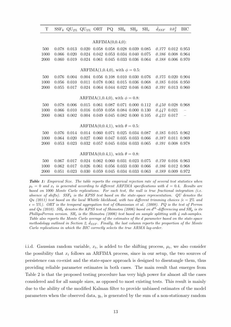
combinations of the ARMA terms, as in Qu (2011). Table 1 reports the empirical rejection
frequencies at 5% nominal level of the various test statistics considered. It emerges that the
modified Kalman filter estimates of the two-component model in (7) leads to estimates of
the fractional parameter (and of the other ARFIMA parameters) that are close to the true
ones although the level shift process is not in the DGP. Indeed, the Monte Carlo average of
the estimates of the fractional parameter based on the state-space representation, denoted as
dSSF , is very close to the true value in all cases. The Monte Carlo average of the estimates of
the other parameters are not reported due to space constraints but they are available upon
request to the authors. Moreover, the Bayesian information criterion selects the correct
number of ARMA terms in more than 95% of the cases for most the DGPs considered. At
the same time, the estimates of π and σ2δ are such that their product is very small, meaning
that the estimated shift component is negligible if compared to the ARFIMA component.
This makes the empirical size of the SSFk test very close to the nominal value, with a slight
over-rejection rate when T = 500. In particular, the rejection rate is higher than 5% when
xt is very persistent, thus making difficult to distinguish between fractional integration and
random level shift in samples that are not particularly long. The other reported tests have
also good size properties, although the QU, SHk and SHp tests are slightly conservative.
Overall, the empirical size of the proposed testing strategy is in line with that of the other
tests and in line with the findings in Qu (2011) and Leccadito et al. (2015).
3.2 Power
The major advantage of the proposed procedure arises when looking at the empirical power
of the test, i.e. when π0 · σ2δ,0 > 0. In line with Qu (2011, p.430), we consider a signal,
xt, contaminated by a non-stationary random level shifts trend process yt = xt + µt, where
µt = µt−1 + γtδt and δt ∼ N(0, 5), γt ∼ Bern(6.1/T ). As noted by Qu (2011), when xt is
i.i.d. standard Gaussian, this parameter configuration is such that the implied degree of
fractional integration of yt is close to 0.4. Therefore in this setup the generated series has
the same degree of long memory as the one used to analyze the size of the tests in Table
1 when yt is a purely fractional process. In addition to the setup in Qu (2011), where an
12
T SSFk QU2% QU5% ORT PQ SHk SHp SHs dSSF πσ2δ BIC
ARFIMA(0,0.4,0):
500 0.078 0.013 0.020 0.058 0.058 0.028 0.039 0.085 0.377 0.012 0.9531000 0.066 0.020 0.024 0.042 0.053 0.034 0.040 0.075 0.386 0.008 0.9642000 0.060 0.019 0.024 0.061 0.045 0.033 0.036 0.064 0.388 0.006 0.970
ARFIMA(1,0.4,0), with ϕ = 0.5:
500 0.076 0.004 0.004 0.056 0.108 0.010 0.030 0.076 0.375 0.020 0.9041000 0.056 0.010 0.011 0.078 0.061 0.015 0.036 0.068 0.385 0.016 0.9502000 0.055 0.017 0.024 0.064 0.044 0.022 0.046 0.063 0.391 0.013 0.960
ARFIMA(1,0.4,0), with ϕ = 0.8:
500 0.078 0.006 0.015 0.061 0.087 0.071 0.000 0.112 0.450 0.028 0.9681000 0.066 0.010 0.016 0.059 0.058 0.084 0.000 0.130 0.447 0.021 –2000 0.063 0.002 0.004 0.049 0.045 0.082 0.000 0.105 0.423 0.017 –
ARFIMA(0,0.4,1), with θ = 0.5:
500 0.076 0.014 0.014 0.060 0.071 0.025 0.034 0.087 0.385 0.015 0.9621000 0.064 0.020 0.027 0.060 0.047 0.035 0.033 0.066 0.387 0.011 0.9692000 0.053 0.023 0.032 0.057 0.045 0.034 0.033 0.065 0.391 0.008 0.978
ARFIMA(0,0.4,1), with θ = 0.8:
500 0.067 0.017 0.024 0.062 0.060 0.031 0.023 0.075 0.370 0.016 0.9631000 0.062 0.017 0.026 0.061 0.056 0.033 0.030 0.066 0.386 0.012 0.9682000 0.051 0.023 0.030 0.059 0.045 0.034 0.033 0.063 0.389 0.009 0.972
Table 1: Empirical Size. The table reports the empirical rejection rate of several test statistics whenµt = 0 and xt is generated according to different ARFIMA specifications with d = 0.4. Results arebased on 1000 Monte Carlo replications. For each test, the null is true fractional integration (i.e.absence of shifts). SSFk is the KPSS test based on the state-space representation. QU denotes theQu (2011) test based on the local Whittle likelihood, with two different trimming choices (ϵ = 2% andϵ = 5%). ORT is the temporal aggregation test of Ohanissian et al. (2008). PQ is the test of Perronand Qu (2010). SHk denotes the KPSS test of Shimotsu (2006) based on dth-differencing and SHp is itsPhillipsPerron version. SHs is the Shimotsu (2006) test based on sample splitting with 4 sub-samples.Table also reports the Monte Carlo average of the estimates of the d parameter based on the state-spacemethodology outlined in Section 2, dSSF . Finally, the last column reports the proportion of the MonteCarlo replications in which the BIC correctly selects the true ARMA lag-order.
i.i.d. Gaussian random variable, xt, is added to the shifting process, µt, we also consider
the possibility that xt follows an ARFIMA process, since in our setup, the two sources of
persistence can co-exist and the state-space approach is designed to disentangle them, thus
providing reliable parameter estimates in both cases. The main result that emerges from
Table 2 is that the proposed testing procedure has very high power for almost all the cases
considered and for all sample sizes, as opposed to most existing tests. This result is mainly
due to the ability of the modified Kalman filter to provide unbiased estimates of the model
parameters when the observed data, yt, is generated by the sum of a non-stationary random
13
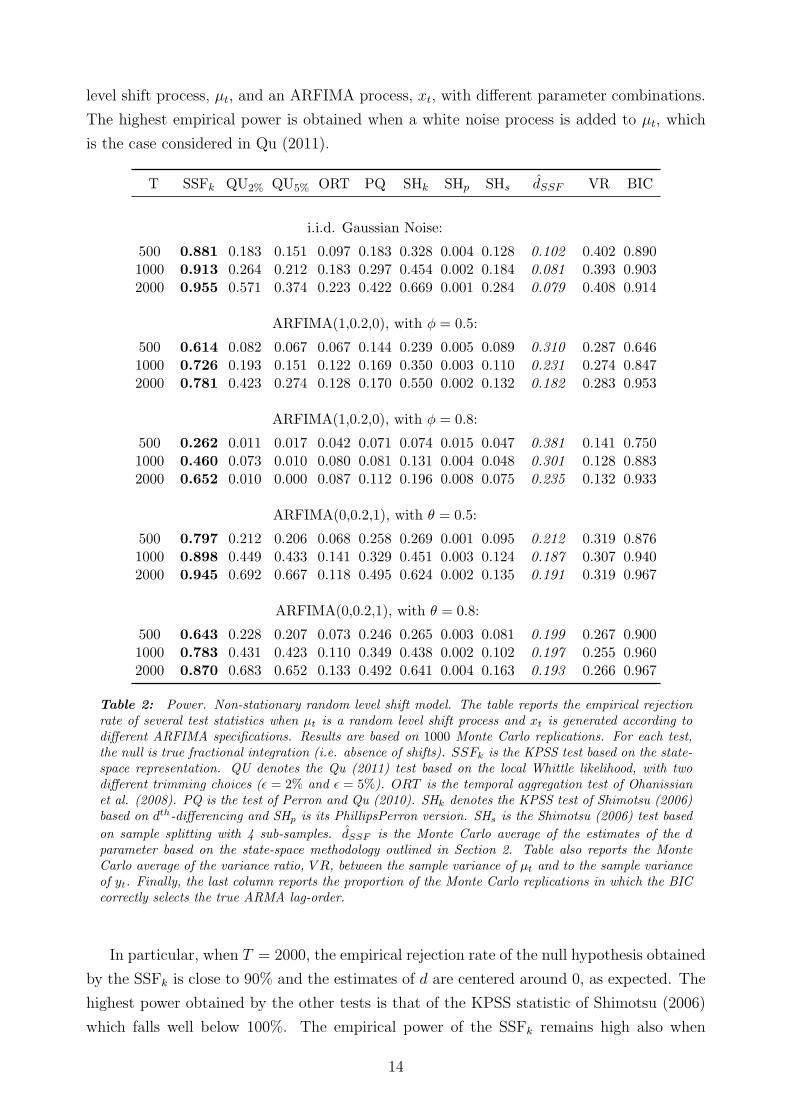
level shift process, µt, and an ARFIMA process, xt, with different parameter combinations.
The highest empirical power is obtained when a white noise process is added to µt, which
is the case considered in Qu (2011).
T SSFk QU2% QU5% ORT PQ SHk SHp SHs dSSF VR BIC
i.i.d. Gaussian Noise:
500 0.881 0.183 0.151 0.097 0.183 0.328 0.004 0.128 0.102 0.402 0.8901000 0.913 0.264 0.212 0.183 0.297 0.454 0.002 0.184 0.081 0.393 0.9032000 0.955 0.571 0.374 0.223 0.422 0.669 0.001 0.284 0.079 0.408 0.914
ARFIMA(1,0.2,0), with ϕ = 0.5:
500 0.614 0.082 0.067 0.067 0.144 0.239 0.005 0.089 0.310 0.287 0.6461000 0.726 0.193 0.151 0.122 0.169 0.350 0.003 0.110 0.231 0.274 0.8472000 0.781 0.423 0.274 0.128 0.170 0.550 0.002 0.132 0.182 0.283 0.953
ARFIMA(1,0.2,0), with ϕ = 0.8:
500 0.262 0.011 0.017 0.042 0.071 0.074 0.015 0.047 0.381 0.141 0.7501000 0.460 0.073 0.010 0.080 0.081 0.131 0.004 0.048 0.301 0.128 0.8832000 0.652 0.010 0.000 0.087 0.112 0.196 0.008 0.075 0.235 0.132 0.933
ARFIMA(0,0.2,1), with θ = 0.5:
500 0.797 0.212 0.206 0.068 0.258 0.269 0.001 0.095 0.212 0.319 0.8761000 0.898 0.449 0.433 0.141 0.329 0.451 0.003 0.124 0.187 0.307 0.9402000 0.945 0.692 0.667 0.118 0.495 0.624 0.002 0.135 0.191 0.319 0.967
ARFIMA(0,0.2,1), with θ = 0.8:
500 0.643 0.228 0.207 0.073 0.246 0.265 0.003 0.081 0.199 0.267 0.9001000 0.783 0.431 0.423 0.110 0.349 0.438 0.002 0.102 0.197 0.255 0.9602000 0.870 0.683 0.652 0.133 0.492 0.641 0.004 0.163 0.193 0.266 0.967
Table 2: Power. Non-stationary random level shift model. The table reports the empirical rejectionrate of several test statistics when µt is a random level shift process and xt is generated according todifferent ARFIMA specifications. Results are based on 1000 Monte Carlo replications. For each test,the null is true fractional integration (i.e. absence of shifts). SSFk is the KPSS test based on the state-space representation. QU denotes the Qu (2011) test based on the local Whittle likelihood, with twodifferent trimming choices (ϵ = 2% and ϵ = 5%). ORT is the temporal aggregation test of Ohanissianet al. (2008). PQ is the test of Perron and Qu (2010). SHk denotes the KPSS test of Shimotsu (2006)based on dth-differencing and SHp is its PhillipsPerron version. SHs is the Shimotsu (2006) test based
on sample splitting with 4 sub-samples. dSSF is the Monte Carlo average of the estimates of the dparameter based on the state-space methodology outlined in Section 2. Table also reports the MonteCarlo average of the variance ratio, V R, between the sample variance of µt and to the sample varianceof yt. Finally, the last column reports the proportion of the Monte Carlo replications in which the BICcorrectly selects the true ARMA lag-order.
In particular, when T = 2000, the empirical rejection rate of the null hypothesis obtained
by the SSFk is close to 90% and the estimates of d are centered around 0, as expected. The
highest power obtained by the other tests is that of the KPSS statistic of Shimotsu (2006)
which falls well below 100%. The empirical power of the SSFk remains high also when
14
ARFIMA processes with d = 0.2 are considered for xt. In all cases, the estimates of d are
centered around the true value, confirming the validity of the state-space approach when
both the long memory component and the shifts are present. The power is drastically
reduced when we consider a highly persistent ARFIMA process with ϕ = 0.8. Indeed, as
indicated by the variance ratio (VR, henceforth) reported in the last column of the table,
the variability of the shift process relative to the total variability of yt is only one third of
that of the white-noise case. It follows that it is relatively more difficult to conduct precise
inference on the shift process when the ARFIMA series is more persistent, and this impacts
on the empirical power of the SSFk test. As noted by Grassi and Santucci de Magistris
(2014), the estimates of the parameter d become more imprecise as the AR parameter gets
closer to 1, but this parameter configuration is rather extreme and not often found in the
real data. For what concerns the misspecification of the ARFIMA dynamics, the selection of
the correct lag order of the ARFIMA is not a concern as the proportion of models correctly
selected by the BIC is generally above 90% when T ≥ 1000. When T = 500, the proportion
is around 70% only when xt follows an ARFIMA(1,d,0) and the estimates of d are slightly
upward biased. Interestingly, the power of the SSFk test is the highest also in this case,
while the power of the other tests slowly increases with T . Indeed, the other semi-parametric
approaches focus on the properties that the series at hands must fulfill to be generated by a
fractionally integrated process while the alternative hypothesis is not necessarily specified in
a parametric form. In other words, a rejection of the null hypothesis of fractional integration
is not informative on the properties of the data generating process (DGP henceforth) under
the alternative. This generally leads to lower empirical powers than those obtained under a
fully specified alternative, and it is particularly true when the sample size is relatively small.
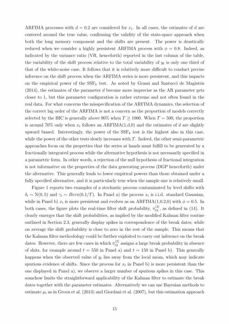
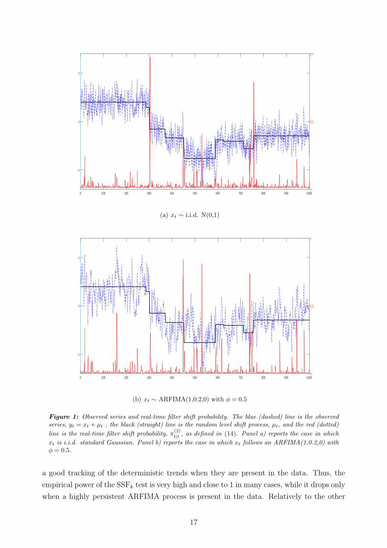
Figure 1 reports two examples of a stochastic process contaminated by level shifts with
δt ∼ N(0, 5) and γt ∼ Bern(6.1/T ). In Panel a) the process xt is i.i.d. standard Gaussian,
while in Panel b) xt is more persistent and evolves as an ARFIMA(1,0.2,0) with ϕ = 0.5. In
both cases, the figure plots the real-time filter shift probability, π(2)t|t , as defined in (14). It
clearly emerges that the shift probabilities, as implied by the modified Kalman filter routine
outlined in Section 2.3, generally display spikes in correspondence of the break dates, while
on average the shift probability is close to zero in the rest of the sample. This means that
the Kalman filter methodology could be further exploited to carry out inference on the break
dates. However, there are few cases in which π(2)t|t assigns a large break probability in absence
of shits, for example around t = 550 in Panel a) and t = 150 in Panel b). This generally
happens when the observed value of yt lies away from the local mean, which may indicate
spurious evidence of shifts. Since the process for xt in Panel b) is more persistent than the
one displayed in Panel a), we observe a larger number of spurious spikes in this case. This
somehow limits the straightforward applicability of the Kalman filter to estimate the break
dates together with the parameter estimates. Alternatively we can use Bayesian methods to
estimate µt as in Groen et al. (2013) and Giordani et al. (2007), but this estimation approach
15
is beyond the scope of the present article. Overall, we can conclude that the large values
of the power associated to the SSPk test are a consequence of the ability of the modified
Kalman filter to account for the probability of shifts and to assign large probabilities of shift
to the break dates in most cases.
3.3 Robustness
The estimation/testing methodology proposed in this paper is based on a fully parametric
specification of the dynamics of the observed variable as the sum of two components, a long
memory one and another characterized by random level shifts. It is therefore important to
assess the robustness of the proposed testing methodology to possible misspecifications of
the shift term. We have already seen that the misspecification of the short-run components
of the ARFIMA can be successfully controlled by adopting a selection method based on
the Bayesian information criterion. In order to assess the robustness of the SSFk test to
different trend processes, the finite sample properties of the SSFk test are also investigated
for other types of trends that can characterize the observed series. In other words, the
estimation/testing procedure outlined in Section 2.3 is carried out under the following DGPs
for µt
1. Stationary random level shifts: µt = (1 − γt)µt−1 + γtδt, with δt ∼ N(0, 1), γt ∼Bern(0.003);
2. Monotonic trend: µt = 3t−0.1;
3. Non-monotonic trend: µt = sin(4πt/T );
The good performance of the SSFk test is confirmed also when an ARFIMA process is
contaminated by a stationary random level shift process, see Table A.1 in the supplementary
material. The power of the SSFk test in detecting the presence of the shift process is the
highest in almost all cases considered. We attribute this performance to the ability of
the state-space method to provide accurate parameter estimates in all cases. Indeed, the
estimates of d are generally centered around the true value also when the µt is misspecified.
Also in this case, we note a low empirical power when xt follows an ARFIMA(1,d,0) with
ϕ = 0.8 as a consequence of the low VR, which is below 10% in all cases and makes very
difficult to identify the source of variation generated by the stationary random level shift
process. However, the empirical power of the SSFk is comparable to that of the semi-
parametric alternatives in this case.
Looking at the cases in which µt follows monotonic or non-monotonic trends, we note that
the SSFk test performs surprisingly well when non-stochastic trends are present in the data,
see Tables A.2 and A.3 in the supplementary material. Although the model specification
is not designed to account for those DGPs, the modified Kalman filter method provides
16
0 100 200 300 400 500 600 700 800 900 1000
-5
0
5
0
0.2
0.4
(a) xt ∼ i.i.d. N(0,1)
0 100 200 300 400 500 600 700 800 900 1000
-5
0
5
0
0.5
1
(b) xt ∼ ARFIMA(1,0.2,0) with ϕ = 0.5
Figure 1: Observed series and real-time filter shift probability. The blue (dashed) line is the observedseries, yt = xt + µt , the black (straight) line is the random level shift process, µt, and the red (dotted)
line is the real-time filter shift probability, π(2)t|t , as defined in (14). Panel a) reports the case in which
xt is i.i.d. standard Gaussian. Panel b) reports the case in which xt follows an ARFIMA(1,0.2,0) withϕ = 0.5.
a good tracking of the deterministic trends when they are present in the data. Thus, the
empirical power of the SSFk test is very high and close to 1 in many cases, while it drops only
when a highly persistent ARFIMA process is present in the data. Relatively to the other
17

semi-parametric tests, the power of the SSFk test is extremely high for the monotonic trend.
For the non-monotonic trend, we observe a good performance of the Qu (2011) test, with
the exclusion of the ARFIMA(1,0.2,0) with ϕ = 0.8. Interestingly, the power of the SSFk
is high even though the VR is relatively low compared to that associated to the random
level-shift processes, as shown in the previous tables.
4 Empirical applications
4.1 Level shifts in volatility and trading volume
We now apply the SSFk test to a number of financial time series for which evidence of long
memory has been documented. In particular, we choose daily bipower-variation and share
turnover, which is the trading volume divided by the number of outstanding shares. The
sample consists of 15 assets traded on NYSE covering the the period between January 2,
2003 and June 28, 2013, for a total of 2640 observations. As it has been widely shown in the
past, the series of realized volatility and bipower-variation are characterized by long-range
dependence, or long memory, see Andersen et al. (2001a) and Martens et al. (2009) among
many others. Analogously, it has been documented that trading volume also displays the
features of a long-range dependent process. For instance, Bollerslev and Jubinski (1999) and
Lobato and Velasco (2000) both report strong evidence that volume exhibits long memory,
as measured by significantly positive fractional integration orders. More recently, Rossi and
Santucci de Magistris (2013) study the common dynamic dependence between volatility
and volume and find evidence of fractional cointegration only for the series belonging to the
bank/financial sector, i.e. those that during the financial crises have experienced a large
upward level shift. It is therefore of interest to be able to formally test, although for now in
an univariate setup only, if volatility and volume are subject to level shifts or if their long-
run dependence is more likely generated by a pure fractional process. The bipower-variation
is constructed using log-returns at 1-minute frequencies as
BPVt =π
2
(M
M − 1
) M∑j=2
|rt,j−1| · |rt,j|, (17)
where rt,j is the j-th log-return on day t and M = 390 is the number of intra-daily ob-
servations associated to 1-minute frequencies. The BPVt estimator converges to the daily
integrated variance, i.e. the instantaneous variance cumulated over daily horizons, and it is
robust to price jumps. The daily turnover is defined as
TRVt =VtSt, (18)
18

where Vt is the trading volume, i.e. number of shares that have been bought and sold within
day t and St is the number of shares available for sale by the general trading public at time t.
The turnover is by construction more robust than trading volume to effects like stock splits
and it does not display large upward trends as Vt. The empirical analysis is carried out on
the log-transformed series, log(BPVt) and log(TRVt) as the model (1) involves unobserved
components that are defined on the entire set of real numbers. Moreover, although the
distributions of bipower-variation and turnover are clearly right-skewed, the distribution of
their logarithms is closer to the Gaussian.
Tables 3 and 4 report the values of the tests for the presence of level shifts in log(BPVt)
and log(TRVt). Following Johansen and Nielsen (2016), we center both log(BPVt) and
log(TRVt) around zero at the origin, by subtracting the first observation, which plays the
role of initial value for µt. The results are not affected by the adoption of other initialization
schemes, e.g. subtracting the sample mean and or an average of the first k observations.
For what concerns log(BPVt), the SSFk test rejects the null hypothesis of absence of shifts
for 8 out of 15 stocks at 5% significance level. Interestingly, the highest values of the tests
are associated with the companies operating in the financial sector, like Bank of America
(BAC), Citygroup (C), JP-Morgan (JPM) and Wells Fargo (WFC). These companies have
been subject to a major financial distress during the 2008-2009 financial crisis, and the values
of BPVt have been extremely high for many months in this period. The test of Perron and
Qu (2010) also seems to find significant evidence of shifts for three out of four volatility series
of the stocks in the bank sector. However, the tests based on semi-parametric specifications
are unable to reject the null hypothesis of fractional integration in most cases. This may
be the consequence of the rather low power of the test, as it emerged in the Monte Carlo
study. Indeed, the local Whittle estimates of d generally lie above the stationary threshold,
i.e. d > 0.5. On the other hand, the estimates obtained with the state-space methodology
are still positive but significantly smaller than 0.5 (with the exception of PG), meaning that
a large portion of the observed long-run dependence is attributed to the random level shifts
(or possibly other slowly-varying trend components).
For what concerns log(TRVt), the SSFk rejects the null hypothesis of absence of shifts
for 13 out of 15 stocks at 5% significance level, and the estimated fractional parameter is
significantly larger than 0 in all cases. Interestingly, there is an almost unanimous agreement
across all tests that the turnover series of BA, HPQ, JPM and PEP present spurious long
memory features, while the assumption of truly long memory for the log(TRVt) of PG is
only rejected by the SHs test. Again, the highest values of the SSFk test are associated with
BAC, C, JPM and WFC. This seems to provide some preliminary motivation to investigate
the long run relationship between volatility and volume being possibly driven by the joint
presence of shifts and not only by a common fractional trend. Indeed, both log(BPVt) and
log(TRVt) may be generated by the combination of a fractional process and a shift (or a
potentially non-linear and smooth trend).
19

SSFk QU2% QU5% ORT PQ SHp SHk SHs dw dSSF
BA 0.638∗ 0.868 0.558 3.035 -0.298 -1.606 0.118 2.881 0.652 0.420BAC 1.735∗ 0.653 0.569 7.415 2.493∗ -0.802 0.226 3.169 0.711 0.412C 2.710∗ 0.421 0.685 7.224 2.589∗ -0.948 0.265 2.064 0.702 0.395CAT 0.318 1.080 0.721 1.286 0.191 -1.656 0.114 7.307 0.707 0.477FDX 0.732∗ 0.601 0.539 1.331 1.177 -1.166 0.195 4.251 0.617 0.373HON 0.355 0.771 0.460 1.099 -0.360 -1.195 0.097 9.070∗ 0.645 0.404HPQ 0.568∗ 0.425 0.540 0.681 -0.455 -2.203 0.078 3.474 0.668 0.339IBM 0.283 0.488 0.845 2.184 0.454 -2.334 0.058 6.114 0.705 0.447JPM 1.419∗ 0.517 0.633 7.361 1.810 -1.607 0.212 3.845 0.716 0.412PEP 0.426 0.365 0.468 4.374 -0.270 -1.664 0.084 6.159 0.699 0.436PG 0.166 0.565 0.670 4.548 0.749 -2.098 0.058 8.335∗ 0.673 0.499T 0.313 0.449 0.670 2.390 -0.410 -0.931 0.087 4.326 0.680 0.429TWX 0.584∗ 0.449 0.553 1.539 -0.079 -1.508 0.080 9.324∗ 0.702 0.450TXN 0.517∗ 0.755 0.314 1.072 -0.492 -1.382 0.123 5.775 0.695 0.442WFC 2.492∗ 0.594 0.368 4.773 2.029∗ -1.110 0.234 2.174 0.740 0.371
Table 3: Empirical application. The table reports the values of several test statistics for thebipower-variations series of 15 assets traded on NYSE. The asterisk denotes rejection of thenull at 5% significance level. SSFk is the KPSS test based on the state-space representation. QUdenotes the Qu (2011) test based on the local Whittle likelihood, with two different trimmingchoices (ϵ = 2% and ϵ = 5%). ORT is the temporal aggregation test of Ohanissian et al.(2008). PQ is the test of Perron and Qu (2010). SHk denotes the KPSS test of Shimotsu(2006) based on dth-differencing and SHp is its PhillipsPerron version. SHs is the Shimotsu
(2006) test based on sample splitting with 4 sub-samples. dw and dSSF are the estimates ofthe fractional parameter obtained with the local Whittle estimator and the state-space methodrespectively.
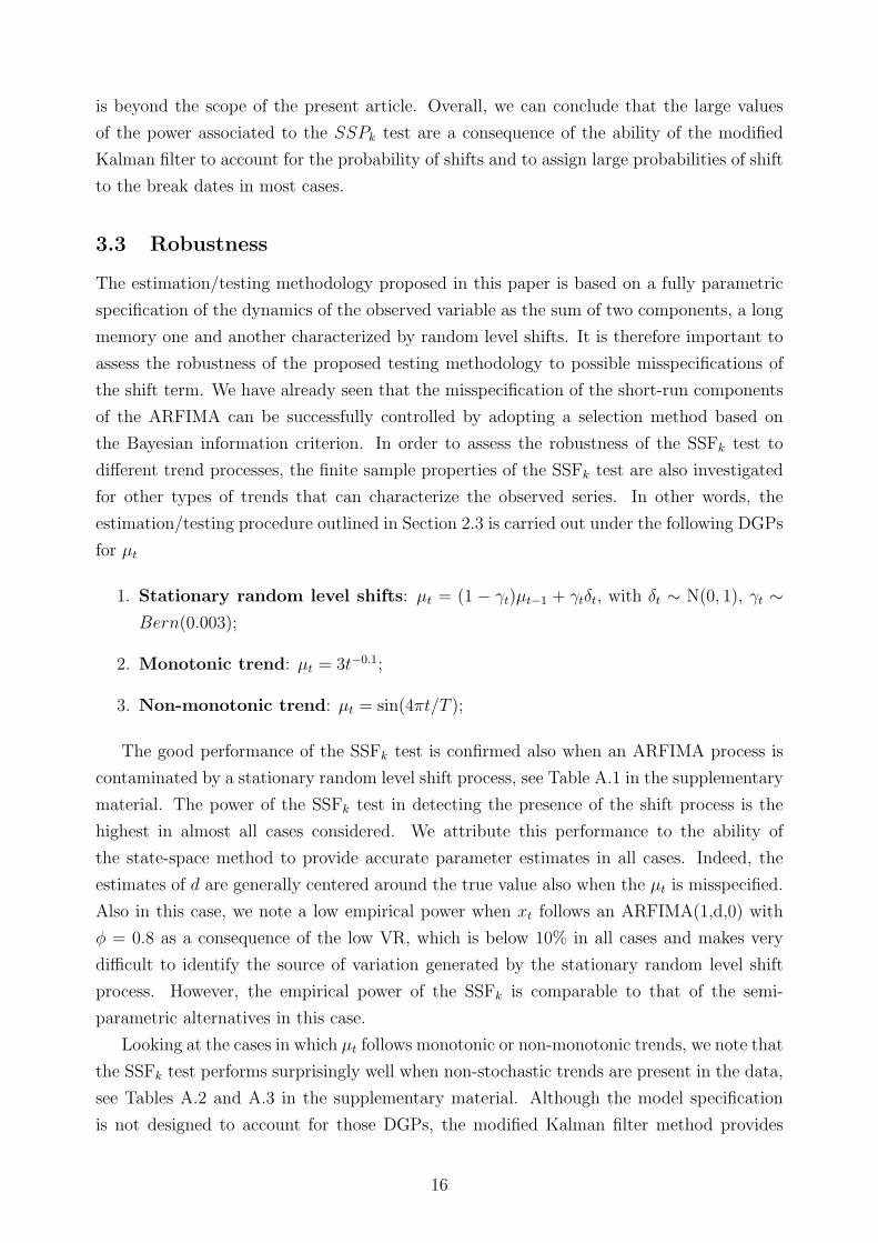
Concluding, Figure 2 plots the observed series of log(BPVt) of BAC and estimated shift
component, µt, obtained given the SSFk estimates. The estimated shift process seems to
follow the largest breaks in the series, which is characterized by a sequence of large increases
starting in the summer of 2007, which is the beginning of the 2007-2009 recession period
according to NBER. The volatility series reaches the highest levels in late 2008, which is
the peak of the subprime financial crisis, while it drops quickly after mid 2009 to a long-run
value that is by far larger than the pre-crisis long-run value. Interestingly, the detrended
series ˜logBPV t = logBPV t − µt, still displays evidence of being a fractional process, with
an associated semiparametric estimate of the fractional parameter d equal to 0.44, a value
that is extremely close to that reported in Table 3. This evidence not only confirms the
ability of the modified Kalman filter to disentangle shifts from the ARFIMA component
thus providing unbiased estimates by a straightforward optimization of the log-likelihood
function of model 7, but it also provides support to the tracking methodology adopted for
the shifts process. In light of the evidence presented in this section, the results in Rossi and
Santucci de Magistris (2013) could be further extended in the direction of a multivariate
long memory model subject to level shifts to be able to account for the contemporaneous
occurrence of breaks in a framework possibly characterized by common fractional trends.
20

SSFk QU2% QU5% ORT PQ SHp SHk SHs dw dSSF
BA 0.767∗ 2.382∗ 1.926∗ 20.43∗ 1.859 -0.356 0.794∗ 0.753 0.394 0.275BAC 9.357∗ 0.918 0.749 5.359 1.673 -0.066 0.563∗ 5.351 0.831 0.262C 5.156∗ 1.699∗ 1.248∗ 6.271 1.268 -0.444 0.291 19.14∗ 0.630 0.304CAT 0.272 1.581∗ 1.283∗ 3.594 1.717 -0.635 0.477∗ 12.55∗ 0.446 0.385FDX 1.255∗ 1.753∗ 1.293∗ 0.066 0.561 -0.507 0.665∗ 3.411 0.357 0.246HON 0.523∗ 1.025 0.641 9.005∗ 1.879 -0.898 0.362 13.30∗ 0.410 0.346HPQ 6.707∗ 2.283∗ 1.884∗ 4.282 2.087∗ 1.060 1.779∗ 15.43∗ 0.425 0.213IBM 0.987∗ 1.015 0.588 3.514 2.084∗ -1.024 0.261 2.333 0.431 0.286JPM 7.063∗ 1.857∗ 1.450∗ 10.81∗ 2.753∗ -0.682 0.516∗ 7.295 0.546 0.261PEP 0.735∗ 1.892∗ 1.201∗ 3.507 2.706∗ -0.345 0.803∗ 0.918 0.427 0.357PG 0.393 0.871 0.703 1.598 0.714 -0.736 0.372 20.84∗ 0.444 0.375T 0.512∗ 0.922 0.499 2.873 1.641 -0.905 0.346 6.204 0.374 0.319TWX 0.510∗ 1.164 1.095 2.954 1.794 -0.390 0.564∗ 21.27∗ 0.397 0.335TXN 0.609∗ 1.392∗ 0.768 1.896 1.439 -0.525 0.528∗ 5.053 0.454 0.331WFC 2.890∗ 1.061 0.497 5.978 2.064∗ -0.641 0.410 11.52∗ 0.723 0.311
Table 4: Empirical application. The table reports the values of several test statistics for thedaily turnover series of 15 assets traded on NYSE. The asterisk denotes rejection of the nullat 5% significance level. SSFk is the KPSS test based on the state-space representation. QUdenotes the Qu (2011) test based on the local Whittle likelihood, with two different trimmingchoices (ϵ = 2% and ϵ = 5%). ORT is the temporal aggregation test of Ohanissian et al.(2008). PQ is the test of Perron and Qu (2010). SHk denotes the KPSS test of Shimotsu(2006) based on dth-differencing and SHp is its PhillipsPerron version. SHs is the Shimotsu
(2006) test based on sample splitting with 4 sub-samples. dw and dSSF are the estimates ofthe fractional parameter obtained with the local Whittle estimator and the state-space methodrespectively.
This extension, coupled with the definition of an efficient method to track the shifting process
given the parameter estimates, is left to future research.
4.2 Level shifts in inflation
The observed persistence in the inflation series is an important issue for economists and
central bankers especially when designing an optimal monetary policy that must take into
account if and at what speed the innovations to the price levels recover to their long-run
mean. Indeed, high persistence in inflation means that a shock to the price level has a long
run effect on the inflation for a long period. Therefore, understanding the source of persis-
tence in inflation is a primary concern since alternative assumptions on the mean-reverting
behavior of the inflation may influence the policies adopted by central banks to control the
general level of prices. Originally, the empirical literature has investigated whether inflation
was better described as a unit-root or as a stationary ARMA process, or a combination of
both, see Kim (1993). More recently, part of the literature has emphasized the fact that
an ARFIMA-type of process could be responsible for the observed slow decay of the auto-
correlation function, see Hassler and Wolters (1995), Sun and Phillips (2004), Sibbertsen
21

Date2004 2005 2006 2007 2008 2009 2010 2011 2012 2013
-2
-1
0
1
2
3
4
5
6
Figure 2: Observed series of log(BPVt) of BAC and estimated shift component. The black-solid lineis the observed series of log(BPVt) of BAC, while the red-dotted line is the estimated shift componentbased on the SSFk estimates.
and Kruse (2009) and Bos et al. (2014) among others. Following the argument of Zaffaroni
(2004), fractional integration in the inflation series is consistent with a sticky-price generat-
ing process as in Calvo (1983). On the other hand, Hsu (2005) suggests that the dynamics
of the inflation series could be characterized by level shifts. Along the same line, Baillie
and Morana (2012) and Bos et al. (1999) model inflation combining an ARFIMA with a
regime-switching term for the long-run mean, finding that the estimates of the fractional
parameters are smaller than those obtained with classic ARFIMA models. In the following,
we formally assess if structural breaks, possibly associated to changes in the monetary policy
of central banks, are responsible for the observed persistence in inflation.
The dataset consists of the monthly de-seasonalized inflation series of the G7 countries
for the period January 1967-July 2016, for a total of 595 observations. To accommodate
the strong empirical evidence that the variability of the inflation rates has diminished after
the mid-80s, a phenomenon known as Great Moderation, model (1) is slightly modified to
account for a break in the variance of the innovation of xt after January 1985. Table 5
reports the values of the tests for the presence of level shifts in the inflation series. For
what concerns the SSFk test, the results are mixed. There is a strong evidence of significant
shifts in the mean of inflation for US, Canada and Japan, while, for the European countries,
the evidence points against the presence of level shifts, with the exception of Italy . In this
case, the SSFk test only marginally rejects the null hypothesis. Interestingly, the estimated
fractional parameter, dSSF , is very high for the European countries and generally close to
the semiparametric estimate, dw. This suggests that the persistence of the inflation of the
European G7 countries can be attributed to a fractional root, such that shocks to the prices
22

SSFk QU2% QU5% ORT PQ SHp SHk SHs dw dSSF
US 1.273∗ 0.734 0.734 1.816 -1.374 -0.342 0.546∗ 9.608∗ 0.7334 0.3347CAN 4.317∗ 0.451 0.451 0.248 -0.552 -0.408 0.553∗ 21.89∗ 0.8289 0.0360UK 0.239 1.209 1.128 4.554 0.832 -0.429 0.449∗ 7.241 0.5474 0.7373GER 0.213 1.116 1.116 0.140 -0.081 -0.378 0.532∗ 3.376 0.8411 0.8195FR 0.369 0.883 0.883 2.728 0.914 -0.230 0.697∗ 15.88∗ 0.9360 0.8337ITA 0.577∗ 1.306∗ 1.306∗ 2.555 1.863 -0.035 0.504∗ 0.255 0.7749 0.6173JPN 4.655∗ 1.113 1.113 2.192 0.222 -0.313 0.595∗ 3.252 0.6832 0.0001
Table 5: Empirical application. The table reports the values of several test statistics for themonthly de-seasonalized inflation series of the G7 countries. The asterisk denotes rejection ofthe null at 5% significance level. SSFk is the KPSS test based on the state-space representation.QU denotes the Qu (2011) test based on the local Whittle likelihood, with two different trimmingchoices (ϵ = 2% and ϵ = 5%). ORT is the temporal aggregation test of Ohanissian et al. (2008).PQ is the test of Perron and Qu (2010). SHk denotes the KPSS test of Shimotsu (2006) basedon dth-differencing and SHp is its PhillipsPerron version. SHs is the Shimotsu (2006) test
based on sample splitting with 4 sub-samples. dw and dSSF are the estimates of the fractionalparameter obtained with the local Whittle estimator and the state-space method respectively.
die out at a very low rate. Instead, for Canada and Japan, the presence of significant
level shifts makes the estimated fractional parameter almost null, meaning that the shock
tend to quickly revert to the local mean. Finally for the US, the results suggest the joint
presence of a fractionally integrated term of order d = 0.33 and of a level shift component.
For what concerns the other tests, they generally tend to not-reject the null hypothesis of
true fractional integration, with the exception of the KPSS test of Shimotsu (2006), which
marginally rejects the null hypothesis in all cases. A table with all the parameter estimates
of model (1) for all the G7 countries is in the Supplementary material.
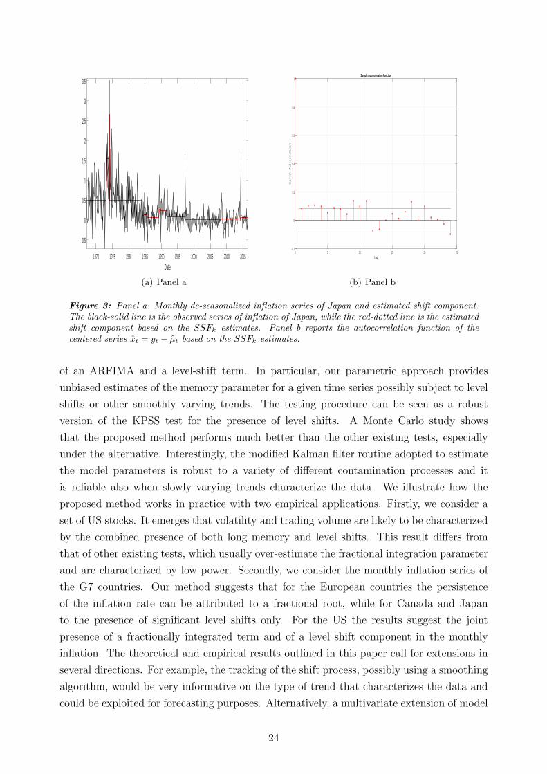
Finally, Panel a of Figure 3 reports the monthly de-seasonalized inflation series of Japan
and the estimated shift component µt based on the estimates of model (1). The figure
highlights the drop in the long-run mean associated with the Great Moderation period
starting from the mid-80s and another drop in the mid-90s, followed by a long period of
average inflation levels close to zero. Looking at the autocorrelation function of the centered
series xt = yt− µt, in Panel b) of Figure 3, we also have a visual confirmation that the breaks
in the long-run mean are the only responsible for the observed persistence in inflation since
the centered series only displays signs of weak dependence.
5 Conclusion
In this paper, we have proposed a robust testing strategy for a fractional process potentially
subject to structural breaks. Contrary to the other tests for true fractional integration
presented so far in the literature, the focus of our approach is on the level shift process. We
propose a flexible state-space parametrization that is able to account for the joint presence
23
Date1970 1975 1980 1985 1990 1995 2000 2005 2010 2015
-0.5
0
0.5
1
1.5
2
2.5
3
3.5
(a) Panel a
Lag0 5 10 15 20 25
Sa
mp
le A
uto
co
rre
latio
n
-0.2
0
0.2
0.4
0.6
0.8
1Sample Autocorrelation Function
(b) Panel b
Figure 3: Panel a: Monthly de-seasonalized inflation series of Japan and estimated shift component.The black-solid line is the observed series of inflation of Japan, while the red-dotted line is the estimatedshift component based on the SSFk estimates. Panel b reports the autocorrelation function of thecentered series xt = yt − µt based on the SSFk estimates.
of an ARFIMA and a level-shift term. In particular, our parametric approach provides
unbiased estimates of the memory parameter for a given time series possibly subject to level
shifts or other smoothly varying trends. The testing procedure can be seen as a robust
version of the KPSS test for the presence of level shifts. A Monte Carlo study shows
that the proposed method performs much better than the other existing tests, especially
under the alternative. Interestingly, the modified Kalman filter routine adopted to estimate
the model parameters is robust to a variety of different contamination processes and it
is reliable also when slowly varying trends characterize the data. We illustrate how the
proposed method works in practice with two empirical applications. Firstly, we consider a
set of US stocks. It emerges that volatility and trading volume are likely to be characterized
by the combined presence of both long memory and level shifts. This result differs from
that of other existing tests, which usually over-estimate the fractional integration parameter
and are characterized by low power. Secondly, we consider the monthly inflation series of
the G7 countries. Our method suggests that for the European countries the persistence
of the inflation rate can be attributed to a fractional root, while for Canada and Japan
to the presence of significant level shifts only. For the US the results suggest the joint
presence of a fractionally integrated term and of a level shift component in the monthly
inflation. The theoretical and empirical results outlined in this paper call for extensions in
several directions. For example, the tracking of the shift process, possibly using a smoothing
algorithm, would be very informative on the type of trend that characterizes the data and
could be exploited for forecasting purposes. Alternatively, a multivariate extension of model
24
(1) would allow to distinguish and test the hypothesis of fractional cointegration in a context
characterized by common and idiosyncratic level shifts.
References
Andersen, T. G., Bollerslev, T., Diebold, F. X., and Ebens, H. (2001a). The distribution of
stock return volatility. Journal of Financial Economics, 61:43–76.
Andersen, T. G., Bollerslev, T., Diebold, F. X., and Labys, P. (2001b). The distribution of
exchange rate volatility. Journal of the American Statistical Association, 96:42–55.
Baillie, R. T., Chung, C. F., and Tieslau, M. A. (1996). Analysing inflation by the fraction-
ally integrated ARFIMA-GARCH model. Journal of Applied Econometrics, 11:23–40.
Baillie, R. T. and Morana, C. (2012). Adaptive ARFIMA models with applications to
inflation. Economic Modelling, 29(6):2451–2459.
Beran, J., Bhansali, R., and Ocker, D. (1998). On unified model selection for stationary and
nonstationary short- and long-memory autoregressive processes. Biometrika, 85:921–934.
Berenguer-Rico, V. and Gonzalo, J. (2014). Summability of stochastic processes: A gener-
alization of integration for non-linear processes. Journal of Econometrics, 178:331–341.
Bollerslev, T. and Jubinski, D. (1999). Equity trading volume and volatility: Latent in-
formation arrivals and common long-run dependencies. Journal of Business & Economic
Statistics, 17:9–21.
Bos, C. S., Franses, P., and Ooms, M. (1999). Long memory and level shifts: Re-analyzing
inflation rates. Empirical Economics, 24:427–449.
Bos, C. S., Koopman, S. J., and Ooms, M. (2014). Long memory with stochastic variance
model: A recursive analysis for US inflation. Computational Statistics and Data Analysis,
76:144 – 157.
Calvo, G. A. (1983). Staggered prices in a utility-maximizing framework. Journal of mon-
etary Economics, 12:383–398.
Chan, N. and Palma, W. (1998). State space modeling of long-memory processes. Annals
of Statistics, 26:719–740.
Christensen, B. J. and Varneskov, R. T. (2015). Medium band least squares estimation
of fractional cointegration in the presence of low-frequency contamination. CREATES
research papers, Forthcoming on the Journal of Econometrics.
Dahlhaus, R. (1989). Efficient parameter estimation for self-similar processes. Annals of
Statistics, 17:1749–1766.
25
Diebold, F. X., Husted, S., and Rush, M. (1991). Real exchange rates under the gold
standard. Journal of Political Economy, 99:1252–1271.
Diebold, F. X. and Inoue, A. (2001). Long memory and regime switching. Journal of
Econometrics, 105:131–159.
Dolado, J., Gonzalo, J., and Mayoral, L. (2008). Wald tests of i(1) against i(d) alternatives:
Some new properties and an extension to processes with trending components. Studies in
Nonlinear Dynamics & Econometrics, 12:1562–1562.
Durbin, J. and Koopman, S. J. (2012). Time series analysis by state space methods. Num-
ber 38. Oxford University Press.
Fox, R. and Taqqu, M. S. (1986). Large-sample properties of parameter estimates for strongly
dependent stationary gaussian series. Annals of Statistics, 14:517–532.
Giordani, P., Kohn, R., and van Dijk, D. (2007). A unified approach to nonlinearity, struc-
tural change, and outliers. Journal of Econometrics, 137:112–133.
Granger, C. W. J. (1980). Long memory relationships and the aggregation of dynamic
models. Journal of Econometrics, 14:227–238.
Granger, C. W. J. and Hyung, N. (2004). Occasional structural breaks and long memory
with application to the S&P 500 absolute stock returns. Journal of Empirical Finance,
11:399–421.
Granger, C. W. J. and Joyeux, R. (1980). An introduction to long-memory time series
models and fractional differencing. Journal of Time Series Analysis, 4:221–238.
Grassi, S. and Santucci de Magistris, P. (2014). When long memory meets the kalman filter:
A comparative study. Computational Statistics and Data Analysis, 76:301–319.
Groen, J. J. J., Paap, R., and Ravazzolo, F. (2013). Real-time inflation forecasting in a
changing world. Journal of Business & Economic Statistics, 31:29–44.
Haldrup, N. and Kruse, R. (2014). Discriminating between fractional integration and spu-
rious long memory. CREATES Research Papers 2014-19, School of Economics and Man-
agement, University of Aarhus.
Harvey, A. and Proietti, T. (2005). Readings in Unobserved Components Models. OUP
Catalogue. Oxford University Press.
Harvey, A. and Streibel, M. (1998). Testing for a slowly changing level with special reference
to stochastic volatility. Journal of Econometrics, 87:167–189.
26
Harvey, A. C. (1991). Forecasting, Structural Time Series Models and the Kalman Filter.
Cambridge Books. Cambridge University Press.
Hassler, U. and Wolters, J. (1995). Long memory in inflation rates: International evidence.
Journal of Business & Economic Statistics, 13:37–45.
Hosking, J. (1981). Fractional differencing. Biometrika, 68:165–76.
Hsu, C.-C. (2005). Long memory or structural changes: An empirical examination on
inflation rates. Economics Letters, 88(2):289–294.
Hurst, H. (1951). Long term storage capacity of reservoirs. Transactions of The American
Society of Civil Engineers, 1:519–543.
Johansen, S. and Nielsen, M. Ø. (2016). The role of initial values in conditional sum-of-
squares estimation of nonstationary fractional time series models. Econometric Theory,
32:1095–1139.
Kim, C.-J. (1993). Unobserved-component time series models with Markov-switching het-
eroscedasticity: Changes in regime and the link between inflation rates and inflation
uncertainty. Journal of Business & Economic Statistics, 11(3):341–349.
Kim, C. J. (1994). Dynamic linear models with Markov-switching. Journal of Econometrics,
60:1–22.
Kim, C. J. and Nelson, C. R. (1999). State-Space Models with Regime Switching: Classical
and Gibbs-Sampling Approaches with Applications, volume 1 of MIT Press Books. The
MIT Press.
Leccadito, A., Rachedi, O., and Urga, G. (2015). True versus spurious long memory: Some
theoretical results and a monte carlo comparison. Econometric Reviews, 34:452–479.
Leybourne, S. J. and McCabe, B. P. M. (1994). A consistent test for a unit root. Journal
of Business & Economic Statistics, 12:157–166.
Ling, S. and McAleer, M. (2010). A general asymptotic theory for time-series models.
Statistica Neerlandica, 64(1):97–111.
Lobato, I. N. and Velasco, C. (2000). Long memory in stock-market trading volume. Journal
of Business & Economic Statistics, 18:410–427.
Mandelbrot, B. (1975). Limit theorems of the self-normalized range for weakly and strongly
dependent processes. Z. Wahrscheinlichkeitstheorie verw. Gebiete, 31:271–285.
Martens, M., Van Dijk, D., and De Pooter, M. (2009). Forecasting S&P 500 volatility: Long
memory, level shifts, leverage effects, day-of-the-week seasonality, and macroeconomic
announcements. International Journal of Forecasting, 25:282–303.
27
McCloskey, A. and Perron, P. (2013). Memory Parameter Estimation In The Presence Of
Level Shifts And Deterministic Trends. Econometric Theory, 29:1196–1237.
Mikosch, T. and Starica, C. (2004). Nonstationarities in financial time series, the long-range
dependence, and the igarch effects. The Review of Economics and Statistics, 86:378–390.
Nyblom, J. and Makelainen, T. (1983). Comparisons of tests for the presence of random
walk coefficients in a simple linear model. Journal of the American Statistical Association,
78:865–864.
Ohanissian, A., Russell, J. R., and Tsay, R. S. (2008). True or spurious long memory? a
new test. Journal of Business & Economic Statistics, 26:161–175.
Perron, P. and Qu, Z. (2010). Long-memory and level shifts in the volatility of stock market
return indices. Journal of Business & Economic Statistics, 28:275–290.
Qu, Z. (2011). A test against spurious long memory. Journal of Business & Economic
Statistics, 29:423–438.
Robinson, P. M. (1995). Log-periodogram regression of time series with long range depen-
dence. The Annals of Statistics, 23:1048–1072.
Rossi, E. and Santucci de Magistris, P. (2013). Long memory and tail dependence in trading
volume and volatility. Journal of Empirical Finance, 22:94–112.
Ruud, P. A. (2000). An introduction to classical econometric theory. Oxford University
Press.
Shephard, N. G. and Harvey, A. C. (1990). On the probability of estimating a deterministic
component in the local level model. Journal of time series analysis, 11:339–347.
Shimotsu, K. (2006). Simple (but effective) tests of long memory versus structural breaks.
Technical report, Working paper, Queen’s University.
Sibbertsen, P. and Kruse, R. (2009). Testing for a break in persistence under long-range
dependencies. Journal of Time Series Analysis, 30(3):263–285.
Sowell, F. (1992). Maximum likelihood estimation of stationary univariate fractionally in-
tegrated time series models. Journal of Econometrics, 53:165–188.
Sun, Y. and Phillips, P. C. (2004). Understanding the fisher equation. Journal of Applied
Econometrics, 19(7):869–886.
Varneskov, R. T. and Perron, P. (2015). Combining long memory and level shifts in modeling
and forecasting the volatility of asset returns. Technical report, Boston University -
Department of Economics.
28

Xiaofeng, S. and Xianyang, Z. (2010). Testing for change points in time series. Journal of
the American Statistical Association, 105:1228–1240.
Zaffaroni, P. (2004). Contemporaneous aggregation of linear dynamic models in large
economies. Journal of Econometrics, 120(1):75–102.
A Appendix
A.1 Summability order of the level shift component µt
In order to study the order of integration of the non-linear process µt defined in (2), we use
the concept of summability as introduced by Berenguer-Rico and Gonzalo (2014).
Definition 1. A stochastic process µt : t ∈ N is said to be summable of order β, or S(β),
if there exists a slowly varying function L(T ) and a deterministic sequence mt, such that
ST =1
T 1/2+βL(T )
T∑t=1
(µt −mt) = Op(1)
where β is the minimum real number that makes ST bounded in probability. Under mild
regularity conditions, it holds that if a process µt is I(β) with d ≥ 0, then it is S(β).
The summability condition of the process µt defined in (2) can be obtained by looking at µt
as a random walk process (analogously to Examples 3 and 5 in Berenguer-Rico and Gonzalo,
2014), where the innovation is zt = γtδt, where γt ∼ Bern(π) and δt ∼ N(0, σ2δ ), so that
E(zt) = E(γt) · E(δt) = π · 0 = 0, (19)
Var(zt) = Var(γt) · Var(δt) + Var(δt) · E(γt)2 +Var(γt) · E(δt)2 (20)
= π(1− π)σ2δ + π2σ2
δ + 0 = π · σ2δ .
Therefore the partial sum
1
T12
1
σδ√π
[Tr]∑t=1
ztd→W (r), (21)
so that zt ∼ S(0) and zt ∼ I(0). Provided that µt =∑T
t=1 zt, then
1
T32
1
σδ√π
[Tr]∑t=1
µtd→∫ r
0
W (r)dr, (22)
29
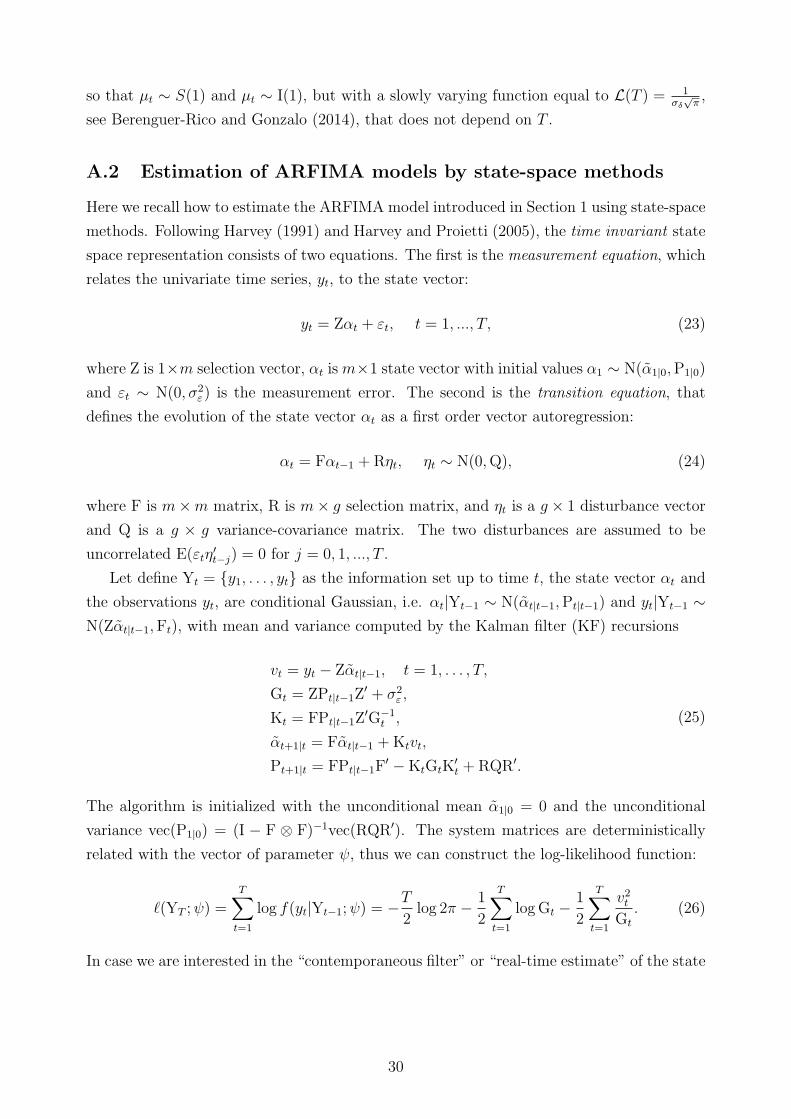
so that µt ∼ S(1) and µt ∼ I(1), but with a slowly varying function equal to L(T ) = 1σδ
√π,
see Berenguer-Rico and Gonzalo (2014), that does not depend on T .
A.2 Estimation of ARFIMA models by state-space methods
Here we recall how to estimate the ARFIMA model introduced in Section 1 using state-space
methods. Following Harvey (1991) and Harvey and Proietti (2005), the time invariant state
space representation consists of two equations. The first is the measurement equation, which
relates the univariate time series, yt, to the state vector:
yt = Zαt + εt, t = 1, ..., T, (23)
where Z is 1×m selection vector, αt ism×1 state vector with initial values α1 ∼ N(α1|0,P1|0)
and εt ∼ N(0, σ2ε) is the measurement error. The second is the transition equation, that
defines the evolution of the state vector αt as a first order vector autoregression:
αt = Fαt−1 +Rηt, ηt ∼ N(0,Q), (24)
where F is m×m matrix, R is m× g selection matrix, and ηt is a g × 1 disturbance vector
and Q is a g × g variance-covariance matrix. The two disturbances are assumed to be
uncorrelated E(εtη′t−j) = 0 for j = 0, 1, ..., T .
Let define Yt = y1, . . . , yt as the information set up to time t, the state vector αt and
the observations yt, are conditional Gaussian, i.e. αt|Yt−1 ∼ N(αt|t−1,Pt|t−1) and yt|Yt−1 ∼N(Zαt|t−1,Ft), with mean and variance computed by the Kalman filter (KF) recursions
vt = yt − Zαt|t−1, t = 1, . . . , T,
Gt = ZPt|t−1Z′ + σ2
ε ,
Kt = FPt|t−1Z′G−1
t ,
αt+1|t = Fαt|t−1 +Ktvt,
Pt+1|t = FPt|t−1F′ −KtGtK
′t +RQR′.
(25)
The algorithm is initialized with the unconditional mean α1|0 = 0 and the unconditional
variance vec(P1|0) = (I − F ⊗ F)−1vec(RQR′). The system matrices are deterministically
related with the vector of parameter ψ, thus we can construct the log-likelihood function:
ℓ(YT ;ψ) =T∑t=1
log f(yt|Yt−1;ψ) = −T2log 2π − 1
2
T∑t=1
logGt −1
2
T∑t=1
v2tGt
. (26)
In case we are interested in the “contemporaneous filter” or “real-time estimate” of the state
30

vector, we have that αt|Yt ∼ N(αt|t,Pt|t), where
αt|t = αt|t−1 + Pt|t−1Z′G−1
t vt,
Pt|t = Pt|t−1 − Pt|t−1Z′G−1
t ZPt|t−1.(27)
Looking at equations (25) and (27), we can notice that the filtering (25) can be obtained
from (27) as follows
αt+1|t = Fαt|t,
Pt+1|t = FPt|tF′ +RQR′.
(28)
Equations (27) together with the prediction error vt and its variance Gt are known as the
“updating step”, while the equations (28) are known as the “prediction step”. To derive the
set of recursions for the model with switching parameters we break down the filtering in those
two steps. The ARFIMA model (3) has the following autoregressive (AR) representation
φ(L)xt = ξt, where
φ(L) = 1−∞∑j=1
φjLj = (1− L)d
Φ(L)
Θ(L), (1− L)d =
∞∑j=0
Γ(j − d)
Γ(j + 1)Γ(−d)Lj.
Its moving average (MA) representation is xt = ζ(L)ξt, where
ζ(L) = 1 +∞∑j=1
ψjLj = (1− L)−d
Θ(L)
Φ(L), (1− L)−d =
∞∑j=0
Γ(j + d)
Γ(j + 1)Γ(d)Lj.
Chan and Palma (1998) show that the exact likelihood function is obtained using the AR
(or MA) representation of order T . In order to make the state-space methods feasible, they
propose to a truncation up to lag m. In particular, the truncated AR(m) representation is
αt = (xt, . . . , xt−m+1)′, Z = (1, 0, ..., 0), σ2
ε = 0,
F =
[φ1 . . . φm
Im−1 0
], R = (1, 0, ..., 0)′, Q = σ2
ξ .(29)
Similarly, the truncated MA(m) representation is
αt = (xt, xt|t−1, . . . , xt+m−1|t−1)′, Z = (1, 0, ..., 0), σ2
ε = 0,
F =
[0 Im
0 0′
], R = (1, ζ1, . . . , ζm)
′, Q = σ2ξ .
(30)
The ML estimator, ψ = argmax ℓ(YT ;ψ), based on the truncated representation, as shown
to be consistent, asymptotically Gaussian and efficient for m = T β with β ≥ 1/2; see Chan
and Palma (1998). Here we adopt the truncated AR(m) representation with m =√T .
Note that the initialization of P1|0 requires to invert a m2 ×m2 matrix, thus to reduce the
31

computational complexity we set P1|0 equal to the Toeplitz matrix of γ = (γ0, γ1, . . . , γm−1),
where γj are the autocovariances of the long memory process.
A.3 The Kalman filter with level shifts
The standard Kalman filter algorithm can be modified to account for the presence of a
level shift process. Following Kim (1994), we show how to obtain the recursive formulas to
calculate the transition probabilities and the log-likelihood function for model (7) presented
in Section 2.3. The predictive filter transition probability in (11) is obtained as follows
π(i,j)t|t−1 = Pr(St−1 = i, St = j|Yt−1)
= Pr(St = j|St−1 = i) Pr(St−1 = i|Yt−1)
= Pr(St = j) Pr(St−1 = i|Yt−1)
= λjπ(i)t−1|t−1.
Given our model with two state and one transition probability we can express the four
filtering probabilities in compact form
vec(Πt|t−1) =
π π 0 0
0 0 π π
1− π 1− π 0 0
0 0 1− π 1− π
vec(Πt−1|t−1), (31)
where Πt is 2× 2 matrix
Πt =
[π(1,1)t π
(1,2)t
π(2,1)t π
(2,2)t
]. (32)
The conditional probability for the observation in expression (12) is obtained as follows
f(yt|Yt−1) =∑2
i=1
∑2j=1 f(yt|St−1 = i, St = j,Yt−1) Pr(St−1 = i, St = j|Yt−1)
=∑2
i=1
∑2j=1 f(y
(i,j)t |Yt−1)π
(i,j)t|t−1
= vec(Ωt)′vec(Πt|t−1),
(33)
where Ωt in 2× 2 matrix containing the observations’ conditional probabilities
Ωt =
[ω(1,1)t ω
(1,2)t
ω(2,1)t ω
(2,2)t
], ω
(i,j)t = f(y
(i,j)t |Yt−1). (34)
32

The expression (14) is obtained as follows:
π(i,j)t|t = Pr(St−1 = i, St = j|Yt)
= Pr(St−1 = i, St = j|yt,Yt−1)
=f(y
(i,j)t |Yt−1) Pr(St−1=i,St=j|Yt−1)
f(yt|Yt−1)
=f(y
(i,j)t |Yt−1)π
(i,j)t|t−1
f(yt|Yt−1),
this can be express in compact form
vec(Πt|t) =vec(Ωt)⊙ vec(Πt|t−1)
vec(Ωt)′vec(Πt|t−1), (35)
where “⊙” is the Hadamard product.
A.4 Proof of Theorem 1
Proof. Let’s partition the parameter vector ψ = (π, ϑ′)′, where ϑ = (d, ϕ1, . . . , ϕp, θ1, . . . , θq, σ2ξ , σ
2δ )
′.
Define two sets of parameters, ψ(1) and ψ(2). Suppose that
f(yt|Yt−1;ψ(1)) = f(yt|Yt−1;ψ
(2)) (36)
then
2∑i=1
2∑j=1
f(y(i,j)t |Yt−1;ψ
(1))π(i,j)t|t−1(ψ
(1)) =2∑i=1
2∑j=1
f(y(i,j)t |Yt−1;ψ
(2))π(i,j)t|t−1(ψ
(2))
this implies that
f(y(1,1)t |Yt−1;ψ
(1)) =[π(1,1)t|t−1(ψ
(1))]−1
π(1,1)t|t−1(ψ
(2))f(y(1,1)t |Yt−1;ψ
(2)) +[π(1,1)t|t−1(ψ
(1))]−1 [
f(y−(1,1)t |Yt−1;ψ
(2))− f(y−(1,1)t |Yt−1;ψ
(1))](37)
where f(y−(1,1)t |Yt−1;ψ
(1)) and f(y−(1,1)t |Yt−1;ψ
(2)) denote the mixture of densities with the
exclusion of the (1,1) case.
Recall that the RHS of (37) is a density, so that∫∞−∞ f(y
(1,1)t |Yt−1;ψ
(1))dy = 1 and
that∫∞−∞ π
(i,j)t|t−1f(y
(i,j)t |Yt−1;ψ
(1))dy = π(i,j)t|t−1
∫∞−∞ f(y
(i,j)t |Yt−1;ψ
(1))dy since π(i,j)t|t−1(ψ
(1)) =
λjπit−1|t−1(ψ
(1)) does not involve y at time t. Therefore, it must hold that
1 =λ(2)1
λ(1)1
[π(1)t−1|t−1(ψ
(1))]−1
π(1)t−1|t−1(ψ
(2))+[λ(1)1 π
(1)t−1|t−1(ψ
(1))]−1
π−(1,1)t|t−1 (ψ(1))′ι− π
−(1,1)t|t−1 (ψ(2))′ι
,
(38)
where π−(1,1)t|t−1 (ψ(1)) and π
−(1,1)t|t−1 (ψ(2)) are the vectors of predictive filter transition probabilities
33

with the exclusion of the (1,1) case and ι is a 3×1 vector of ones. Given that the parameters
ϑ(1) and ϑ(2) must be equal since the ARFIMA model is identified as there a no canceling
roots in the AR and MA polynomials, it must follow that, to guarantee that π(1,1)t|t−1(ψ
(1)) =
π(1,1)t|t−1(ψ
(2)), then λ(2)1 = λ
(1)1 , that is π(2) = π(1).
A.5 Proof of Theorem 2
Proof. For the proof of consistency, consider the process in first differences, that is
∆yt = xt − xt−1 + δt (39)
so that ∆yt is a stationary process. The state-space representation associated to (39) is
analogous to that in (2.3), where δt is now treated as a measurement error. The estimation
procedure thus follows the same algorithm outlined above by adapting the methodology
of Kim (1994) and Kim and Nelson (1999) to this context. In particular, the conditional
density is a mixture of four densities weighted by a function of the shifting probabilities,
πi,jt . Following Ling and McAleer (2010), the proof of consistency for the ML estimator of
the parameters governing a stationary time-series consists of the verification of the following
conditions.
i. Esupψ∈Ψ[log f(∆yt|Yt−1;ψ)]
<∞.
ii. Eψ0 [log f(∆yt|Yt−1;ψ0)] < ∞ and Eψ0 [log f(∆yt|Yt−1;ψ)] < Eψ0 [log f(∆yt|Yt−1;ψ0)] for
all ψ = ψ0.
iii. limT→∞ supψ∈Ψ | 1T
∑Tt=1 log f(∆yt|Yt−1;ψ)− 1
T
∑Tt=1 log f(∆yt|Yt−1;ψ)| = 0 a.s. where
log f(∆yt|Yt−1;ψ) is log f(∆yt|Yt−1;ψ) with the initial values x0, x−1, . . . , x−m+1, µ0.
We first prove Condition i. Given that log x ≤ x− 1, ∀x > 0, it is sufficient to show that
E[f(∆yt|Yt−1;ψ)] <∞, where
f(∆yt|Yt−1) =2∑i=1
2∑j=1
f(∆y(i,j)t |Yt−1)π
(i,j)t|t−1, (40)
and the observations are conditionally Gaussian
f(∆y(i,j)t |Yt−1) =
[2πG
(i,j)t
]−1/2
exp
[− v
(i,j)2t
2G(i,j)t
]. (41)
In particular, f(∆y(i,j)t |Yt−1) is the density associated to ∆y
(i,j)t and hence is finite, while
π(i,j)t|t−1 are the predictive filter transition probabilities, so they are in the interval [0, 1] by
construction. Therefore, since f(∆yt|Yt−1;ψ) is a density and the function f(∆yt|Yt−1;ψ),
34
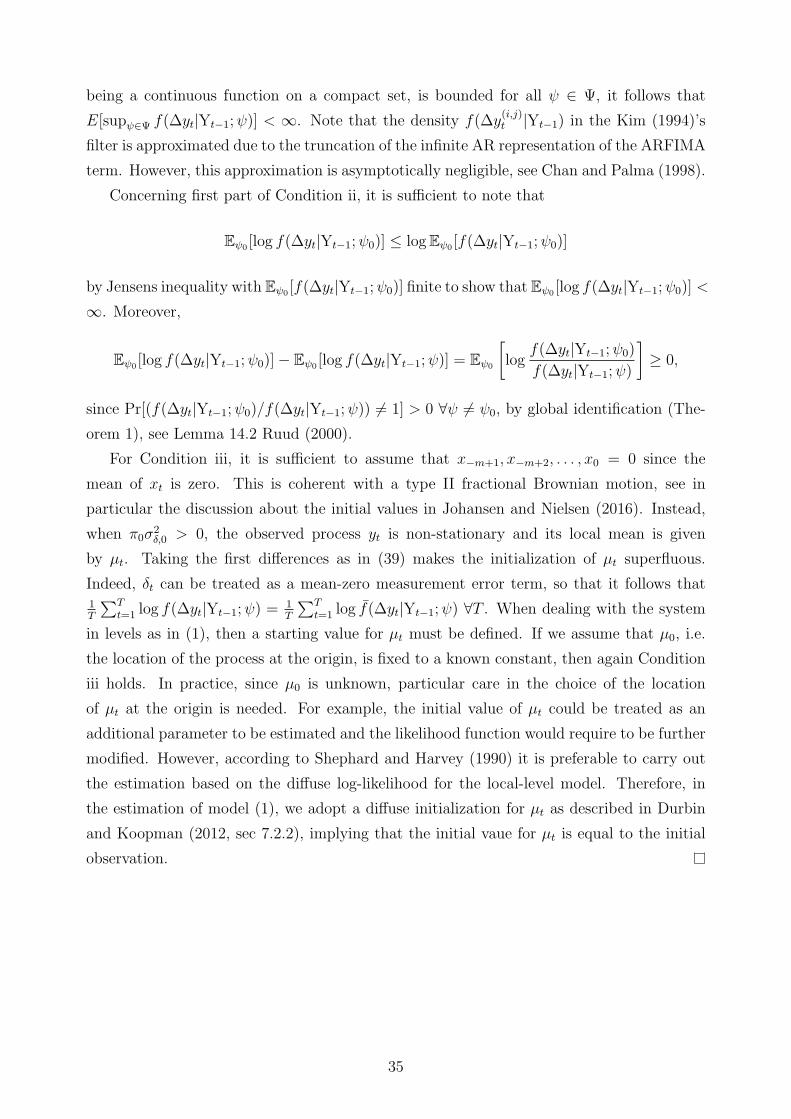
being a continuous function on a compact set, is bounded for all ψ ∈ Ψ, it follows that
E[supψ∈Ψ f(∆yt|Yt−1;ψ)] < ∞. Note that the density f(∆y(i,j)t |Yt−1) in the Kim (1994)’s
filter is approximated due to the truncation of the infinite AR representation of the ARFIMA
term. However, this approximation is asymptotically negligible, see Chan and Palma (1998).
Concerning first part of Condition ii, it is sufficient to note that
Eψ0 [log f(∆yt|Yt−1;ψ0)] ≤ logEψ0 [f(∆yt|Yt−1;ψ0)]
by Jensens inequality with Eψ0 [f(∆yt|Yt−1;ψ0)] finite to show that Eψ0 [log f(∆yt|Yt−1;ψ0)] <
∞. Moreover,
Eψ0 [log f(∆yt|Yt−1;ψ0)]− Eψ0 [log f(∆yt|Yt−1;ψ)] = Eψ0
[log
f(∆yt|Yt−1;ψ0)
f(∆yt|Yt−1;ψ)
]≥ 0,
since Pr[(f(∆yt|Yt−1;ψ0)/f(∆yt|Yt−1;ψ)) = 1] > 0 ∀ψ = ψ0, by global identification (The-
orem 1), see Lemma 14.2 Ruud (2000).
For Condition iii, it is sufficient to assume that x−m+1, x−m+2, . . . , x0 = 0 since the
mean of xt is zero. This is coherent with a type II fractional Brownian motion, see in
particular the discussion about the initial values in Johansen and Nielsen (2016). Instead,
when π0σ2δ,0 > 0, the observed process yt is non-stationary and its local mean is given
by µt. Taking the first differences as in (39) makes the initialization of µt superfluous.
Indeed, δt can be treated as a mean-zero measurement error term, so that it follows that1T
∑Tt=1 log f(∆yt|Yt−1;ψ) =
1T
∑Tt=1 log f(∆yt|Yt−1;ψ) ∀T . When dealing with the system
in levels as in (1), then a starting value for µt must be defined. If we assume that µ0, i.e.
the location of the process at the origin, is fixed to a known constant, then again Condition
iii holds. In practice, since µ0 is unknown, particular care in the choice of the location
of µt at the origin is needed. For example, the initial value of µt could be treated as an
additional parameter to be estimated and the likelihood function would require to be further
modified. However, according to Shephard and Harvey (1990) it is preferable to carry out
the estimation based on the diffuse log-likelihood for the local-level model. Therefore, in
the estimation of model (1), we adopt a diffuse initialization for µt as described in Durbin
and Koopman (2012, sec 7.2.2), implying that the initial vaue for µt is equal to the initial
observation.
35

Research Papers 2016
2016-32: Lasse Bork, Stig V. Møller and Thomas Q. Pedersen: A New Index of Housing Sentiment
2016-33: Joachim Lebovits and Mark Podolskij: Estimation of the global regularity of a multifractional Brownian motion
2017-01: Nektarios Aslanidis, Charlotte Christiansen and Andrea Cipollini: Predicting Bond Betas using Macro-Finance Variables
2017-02: Giuseppe Cavaliere, Morten Ørregaard Nielsen and Robert Taylor: Quasi-Maximum Likelihood Estimation and Bootstrap Inference in Fractional Time Series Models with Heteroskedasticity of Unknown Form
2017-03: Peter Exterkate and Oskar Knapik: A regime-switching stochastic volatility model for forecasting electricity prices
2017-04: Timo Teräsvirta: Sir Clive Granger’s contributions to nonlinear time series and econometrics
2017-05: Matthew T. Holt and Timo Teräsvirta: Global Hemispheric Temperatures and Co–Shifting: A Vector Shifting–Mean Autoregressive Analysis
2017-06: Tobias Basse, Robinson Kruse and Christoph Wegener: The Walking Debt Crisis
2017-07: Oskar Knapik: Modeling and forecasting electricity price jumps in the Nord Pool power market
2017-08: Malene Kallestrup-Lamb and Carsten P.T. Rosenskjold: Insight into the Female Longevity Puzzle: Using Register Data to Analyse Mortality and Cause of Death Behaviour Across Socio-economic Groups
2017-09: Thomas Quistgaard Pedersen and Erik Christian Montes Schütte: Testing for Explosive Bubbles in the Presence of Autocorrelated Innovations
2017-10: Jeroen V.K. Rombouts, Lars Stentoft and Francesco Violante: Dynamics of Variance Risk Premia, Investors' Sentiment and Return Predictability
2017-11: Søren Johansen and Morten Nyboe Tabor: Cointegration between trends and their estimators in state space models and CVAR models
2017-12: Lukasz Gatarek and Søren Johansen: The role of cointegration for optimal hedging with heteroscedastic error term
2017-13: Niels S. Grønborg, Asger Lunde, Allan Timmermann and Russ Wermers: Picking Funds with Confidence
2017-14: Martin M. Andreasen and Anders Kronborg: The Extended Perturbation Method: New Insights on the New Keynesian Model
2017-15: Andrea Barletta, Paolo Santucci de Magistris and Francesco Violante: A Non-Structural Investigation of VIX Risk Neutral Density
2017-16: Davide Delle Monache, Stefano Grassi and Paolo Santucci de Magistris: Does the ARFIMA really shift?
Related Documents