correlated averages vs. averaged correlations: demonstrating the ...

Monin and OppenheimerCORRELATED AVERAGES VS. AVERAGED CORRELATIONS

CORRELATED AVERAGES VS. AVERAGEDCORRELATIONS: DEMONSTRATING THE WARMGLOW HEURISTIC BEYOND AGGREGATION

Benoît MoninStanford University

Daniel M. OppenheimerPrinceton University

Three studies demonstrate the warm glow heuristic (Monin, 2003) withoutrelying on aggregated ratings, and illustrate the important distinction be-tween correlating average ratings versus averaging individual correlations.In Study 1, we re–analyze previous data correlating individual ratings withaggregates from another small sample of raters. In Study 2, we correlate in-dividual familiarity ratings with normed attractiveness from a large sampleof raters (n > 2,500). Study 3 bypasses the issue of aggregates altogether byhaving participants provide both attractiveness and familiarity ratings andcomputing correlations within participants. Despite this more conserva-tive approach, the results of all three studies support the existence of thebeautiful–is–familiar phenomenon.

It is great to be good–looking. The mere fact of being physically at-tractive apparently improves one’s life outcomes significantly.For example, attractive people are more likely to be helped(Chaiken, 1979), less likely to get punished (Downs & Lyons,1991), and tend to earn more money (Hamermesh & Biddle, 1994).People make all kinds of positive inferences based on attractive-

257

Social Cognition, Vol. 23, No. 3, 2005, pp. 257-278

The second author was supported by a National Science Foundation graduate researchfellowship. We would like to thank Peter Finlayson for his help in collecting data for Study2, and Dan Yarlett for his help in collecting data for Study 3.

Address correspondence to Benoît Monin, Department of Psychology, Jordan Hall,Stanford University, Stanford, CA 94305; E-mail: [email protected].

ness alone: Attractive people seem more intelligent, more suc-cessful, more socially skilled, better adjusted, and in general arethought to possess more desirable qualities (Dion, Berscheid, &Walster, 1972; Eagly, Ashmore, Makhijani, & Longo, 1991).

Recently, it was discovered that the impact of attractivenessgoes beyond personality inferences, and can actually influencewhether we think we have seen a face before: Attractive peopleseem more familiar, and are more likely to be recognized, even onfirst encounter (Vokey & Read, 1992; Monin, 2003). In line with re-cent findings suggesting that positivity can cue familiarity (Gar-cia–Marques, Mackie, Claypool, & Garcia–Marques, 2004),Monin attributed this beautiful–is–familiar effect to a “warmglow heuristic” in which people use positive affective reactions tostimuli to infer familiarity (Monin, 2003; Corneille, Monin, &Pleyers, in press). In support of this interpretation, not only do at-tractive faces look familiar, but positive words are also morelikely to seem familiar than neutral or negative words. This inter-play between cognition and affect was foreshadowed by Zajonc(1980) when he proposed that our first reaction to stimuli isaffective and that this first reaction colors subsequent judgments.

However, some demonstrations of the phenomenon exhibit apossible shortcoming. For example, Monin (2003, Study 1)showed a set of photographs to two groups of participants anddemonstrated that the average rating of familiarity by a group of40 judges correlated highly with the average rating of attractive-ness by another group of 34 judges (r = .64). Subsequent studiesused more sophisticated techniques, but retained the feature thataverage ratings on a first dimension by one group are correlatedwith average ratings on a second dimension by another group.This approach provides good evidence that if a given picture israted as attractive, it is likely to be rated as familiar. However, cor-relating these group aggregates falls short of demonstrating theprocess assumed to underlie the warm glow heuristic at the levelof the individual: It was assumed that if a picture is attractive for agiven participant, it should also be more familiar to him or her.Using the picture as the unit of analysis does not afford the oppor-tunity to test this phenomenon at the individual level as it tests thecorrelation of averages, rather than looking at averages ofcorrelations.

258 MONIN AND OPPENHEIMER

AVERAGE CORRELATIONS VERSUSCORRELATION OF AVERAGES

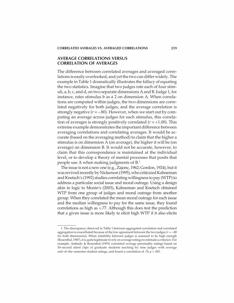
The difference between correlated averages and averaged corre-lations is easily overlooked, and yet the two can differ widely. Theexample in Table 1 dramatically illustrates the fallacy of equatingthe two statistics. Imagine that two judges rate each of four stim-uli, a, b, c, and d, on two separate dimensions A and B. Judge 1, forinstance, rates stimulus b as a 2 on dimension A. When correla-tions are computed within judges, the two dimensions are corre-lated negatively for both judges, and the average correlation isstrongly negative (r = –.80). However, when we start out by com-puting an average across judges for each stimulus, this correla-tion of averages is strongly positively correlated (r = +1.00). Thisextreme example demonstrates the important difference betweenaveraging correlations and correlating averages. It would be ac-curate (based on the averaging method) to claim that the higher astimulus is on dimension A (on average), the higher it will be (onaverage) on dimension B. It would not be accurate, however, toclaim that this correspondence is maintained at the individuallevel, or to develop a theory of mental processes that posits thatpeople use A when making judgments of B.1

The issue is not a new one (e.g., Zajonc, 1962; Gordon, 1924), but itwas revived recently by Nickerson (1995), who criticized Kahnemanand Knetsch’s (1992) studies correlating willingness to pay (WTP) toaddress a particular social issue and moral outrage. Using a designakin in logic to Monin’s (2003), Kahneman and Knetsch obtainedWTP from one group of judges and moral outrage from anothergroup. When they correlated the mean moral outrage for each issueand the median willingness to pay for the same issue, they foundcorrelations as high as +.77. Although this does test the predictionthat a given issue is more likely to elicit high WTP if it also elicits

CORRELATED AVERAGES VS. AVERAGED CORRELATIONS 259

1. The discrepancy observed in Table 1 between aggregated correlation and correlatedaggregation is exacerbated because of the low agreement between the two judges (r = –.80for both dimensions). When reliability between judges is assessed to be high enough(Rosenthal, 1987), it is quite legitimate to rely on average ratings to estimate a criterion. Forexample, Ambady & Rosenthal (1993) correlated average personality ratings based on30–second silent clips of graduate students teaching by nine judges with averageend–of–the–semester student ratings, and found a correlation of .76, p < .001.

moral outrage, Nickerson argues that it leaves out whether moraloutrage is highly correlated to WTP at the level of the individual. Shealso provides the formula relating aggregated correlations and cor-relations of aggregates (see Appendix).

A between–group averaging design such as Monin’s (2003)Study 1 assumes two things: that participants agree on ratings ofattractiveness and familiarity (the intraclass correlation coeffi-cient for attractiveness was .94, and for familiarity it was .78.), andalso that the correlation between the two dimensions is not stron-ger within individuals than it is across individuals. If the formerassumption is violated, then the correlation of averages is anoverestimation of the average of correlations. If the latter assump-tion is violated, then the correlation of averages is anunderestimation of the average of correlations.

THE PRESENT STRATEGY

The problem with using exclusively aggregated data is that itdoes not take into account inter–individual differences and in ef-fect treats sample aggregates as population values. This articleendeavors to re–introduce variability in the estimate of the beau-


TABLE 1. Simulation Demonstrating the Possible Disjunction between a Correlation ofAverages, r (CA) = +1.00, and an Average of Correlations, r (AC) = –.80.

Stimulus

a b c d

Judge 1 Dimension A 0 2 4 6

Dimension B 6 2 4 0 r = –.80

Judge 2 Dimension A 6 2 4 0

Dimension B 0 2 4 6 r = –.80

Aggregated ratings Dimension A 3 2 4 3

Dimension B 3 2 4 3 r (CA) = +1.00

r (AC) = –.80

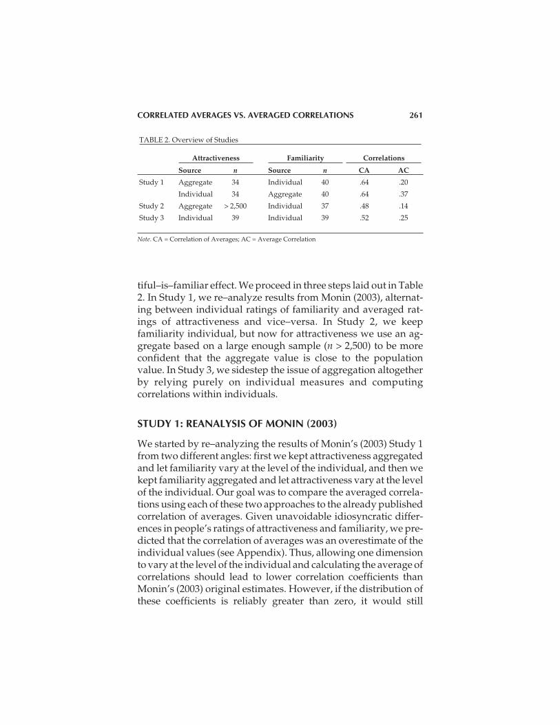
tiful–is–familiar effect. We proceed in three steps laid out in Table2. In Study 1, we re–analyze results from Monin (2003), alternat-ing between individual ratings of familiarity and averaged rat-ings of attractiveness and vice–versa. In Study 2, we keepfamiliarity individual, but now for attractiveness we use an ag-gregate based on a large enough sample (n > 2,500) to be moreconfident that the aggregate value is close to the populationvalue. In Study 3, we sidestep the issue of aggregation altogetherby relying purely on individual measures and computingcorrelations within individuals.

STUDY 1: REANALYSIS OF MONIN (2003)

We started by re–analyzing the results of Monin’s (2003) Study 1from two different angles: first we kept attractiveness aggregatedand let familiarity vary at the level of the individual, and then wekept familiarity aggregated and let attractiveness vary at the levelof the individual. Our goal was to compare the averaged correla-tions using each of these two approaches to the already publishedcorrelation of averages. Given unavoidable idiosyncratic differ-ences in people’s ratings of attractiveness and familiarity, we pre-dicted that the correlation of averages was an overestimate of theindividual values (see Appendix). Thus, allowing one dimensionto vary at the level of the individual and calculating the average ofcorrelations should lead to lower correlation coefficients thanMonin’s (2003) original estimates. However, if the distribution ofthese coefficients is reliably greater than zero, it would still


TABLE 2. Overview of Studies

Attractiveness Familiarity Correlations

Source n Source n CA AC

Study 1 Aggregate 34 Individual 40 .64 .20

Individual 34 Aggregate 40 .64 .37

Study 2 Aggregate > 2,500 Individual 37 .48 .14

Study 3 Individual 39 Individual 39 .52 .25

Note. CA = Correlation of Averages; AC = Average Correlation

provide support for the “beautiful-is-familiar effect” under moreconservative conditions.

METHOD

Eighty pictures (40 from each gender) were taken from a yearbookand arranged on four sheets. Participants rated the 80 pictures on a 1to 10 scale either on attractiveness (n = 34) or on familiarity, definedas the confidence that they had seen the person on the picture be-fore (n = 40). Participants rating familiarity were led to believethat half the pictures were of students still on campus. In realityall pictures were taken from years prior to our respondents’ pres-ence on campus; thus the targets were all new.

RESULTS

Correlation of Averages. As in Monin (2003), we started by com-puting for each picture the average attractiveness across 34judges and the average familiarity across 40 judges. When these80 pairs are correlated using picture as the level of analysis wefind, as previously reported, a correlation of averages that is quitehigh, r = .64, p < .001.

Average of Correlations. To move one step away from aggre-gates, we first took the average attractiveness for each picture,used that as a normed value, and generated the correlation be-tween each of the 40 judges’ familiarity ratings and this normscore. This produces 40 correlation coefficients. The average ofthese correlation coefficients is much lower than the correlation ofaverages, M = .20, SD = 15, though significantly greater than zero,95% C.I. = [.16; .26]. Observing the distribution of correlationscores (see Figure 1a) reveals that whereas some participants ex-hibit high correlation coefficients that look like the correlation ofaverages, others show a much lower association between individ-ual familiarity and aggregated attractiveness, with somerespondents even exhibiting a negative correlation coefficient.

The other way to approach this data is to take the average famil-iarity for each picture, use that as a normed value, and generatethe correlation between each of the 34 judges’ attractiveness rat-


ings and this norm score. This produces 34 (all positive) correla-tion scores (see Figure 1b), M = .37, SD = .11, with a 95% C.I. of [.33;.41].

DISCUSSION

This re–analysis provides an informative reconsideration of previ-ous data. Such a mixed analysis seemed a salutary first approach tothe issue of aggregation. We kept one dimension aggregated, but letthe other vary with each participant. As discussed by Nickerson’s(1995) analysis, and given some predictable disagreements in rat-


FIGURE 1a. Distribution of individual correlations between aggregated attractiveness (n = 34)and individual ratings of familiarity (Study 1).

ings among judges, average correlations were lower than correlatedaverages. This suggests that the correlation reported in Monin (2003)may be an overestimation of the link between attractiveness and fa-miliarity at the individual level. However, the average correlationwas significantly greater than zero. Thus we demonstrated thebeautiful–is–familiar effect even with this more conservative test.

We used “mixed” correlations in this re–analysis, with one di-mension aggregated and one at the level of the individual. Thelogic of aggregation is to get an estimate of a population norm. Al-though this first demonstration has the desirable feature that wecan switch around which dimension was aggregated, it would bepreferable in order to compute mixed correlations to obtain first


FIGURE 1b. Distribution of individual correlations between aggregated familiarity (n = 40) andindividual ratings of attractiveness (Study 1).

normed values from a larger sample to obtain a better estimate ofpopulation values. Aggregates in Study 1 are based on 40 respon-dents at the most. Study 2 again uses the logic of mixed correla-tions but uses attractiveness ratings from a much larger sample toaddress this issue.

STUDY 2: AM I HOT OR NOT?

This second study used a mixed design similar to that used inStudy 1, but used a much larger sample to generate a norm ofattractiveness ratings. The larger sample was gathered by rely-ing on the website amihotornot.com, on which users post theirphotograph to be rated on a single scale of attractiveness bythousands of visitors. Unlike Study 1, this study does not en-able us to alternate which dimension is aggregated in the anal-ysis (because we do not have access to individual ratings ofattractiveness), but the trade–off is the greater reliability of theattractiveness ratings given the great number of respondents.

METHOD

Participants. Thirty–seven Stanford students took part in this ex-periment for course credit. We removed one participant who didnot seem to believe the cover story and answered “1" on all 90 pic-tures, yielding no usable variability.

Materials and Procedure. Participants engaged in a bogus rec-ognition paradigm (similar to Monin, 2003, Study 4) employingphotographs taken from the site amihotornot.com2. Ninetyphotographs that had each received over 2,500 votes were se-lected, with ten at each level of attractiveness ranging from 1.9to 9.9 in one–unit increments. These photographs were then di-vided into two sets of 45 (with five pictures at each level of at-tractiveness), which were presented in counterbalanced order


2. Amihotornot.com [http://www.amihotornot.com] is a website launched in 2000 byJames Hong and Jim Young on which visitors can view photos posted voluntarily by fel-low users and rate their comeliness on a scale from 1 (Not) to 10 (Hot). On 6/28/04, the siteclaimed that it had received 12,200,000photos and 8 billion votes. It has received numerousmedia mentions and has become a popular culture phenomenon.

to different groups of participants. Participants were told thatthey were in an experiment on subliminal perception, that theywould first see photographs below the threshold of consciousperception, and then would be shown several photographs andwould have to guess which they saw. In reality, they were onlyshown multicolored masks flashed on the screen in rapid succes-sion. All photographs at test were new. Participants rated eachphotograph’s familiarity on a scale from 1 (not at all familiar) to 10(very familiar). It is worth noting that these naturalistic photo-graphs were much richer in content than stimuli ordinarilyused in face recognition, including not only differences ingrooming and expression, but also in framing (some includingthe poser’s body), and context.3

RESULTS

Correlation of Average. We observed the same type of correla-tions between familiarity and liking that we had encountered inprevious studies. When we averaged ratings of familiarity acrossparticipants and correlated this average with the normed attrac-


3. This study included a between–subject manipulation of mood after the first 45 test tri-als: Twenty participants saw a five–minute clip of the television cartoon show The Simpsons(positive), while 17 participants saw a nature video (neutral) of approximately the samelength. Although The Simpsons indeed increased participants’ reported mood state, F(1,35)= 6.2, p < .02, it did not have much impact on familiarity ratings. We conducted a Mood ×Order analysis of covariance on average familiarity ratings in the second block, with aver-age familiarity ratings in the pre–movie recognition task as a covariate, and found no effectof mood, nor an interaction with order, both F(1,31) < 1. Note that the mood manipulationdid not impact significantly correlations collected after the manipulation, t(34) = 1.2, ns.

Though it is not the focus of this article, it is worth discussing the absence of mood ef-fects. In light of findings by Monahan, Murphy, and Zajonc (2000) showing that repeatedexposure leads to generalized mood improvement, we expected that improving people’smood might increase their general sense of familiarity. Yet, despite its ability to changepeople’s reported mood state, our mood manipulation did not lead to higher familiarityratings: Improved mood was not misattributed to increased familiarity for stimuli subse-quently presented. These results suggest that the warm glow heuristic may rely on a dif-fuse positive feeling attached to a given stimuli, but that it shows some specificity as to thesource of the feeling. In other words, positive affect might be attributed to the wrong featureof the stimulus, but it may still need to come from the stimulus itself (for another exampleof the limits of misattribution, see Winkielman, Zajonc, & Schwarz, 1997). Given its tangen-tial nature and to simplify our presentation, we ignore this variable in the rest of the article.

tiveness from the website, we observed a high positive correla-tion (r = .48, p < .001).

Average of Correlations. When we computed an individual cor-relation for each participant between their 90 individual ratingsof familiarity and the normed attractiveness scores, we found in-dividual correlations that ranged from –12 to +.49 and an aver-age correlation that was much lower than the correlation ofaverages (M = .14, SD = .16, see Figure 2). This average correla-tion was again significantly different from zero, t(35) = 5.2, p <.001, and the 95% confidence interval for the population coeffi-cient was [+.09; +.19].


FIGURE 2. Distribution of individual correlations between aggregated attractiveness (n > 2,500)and individual ratings of familiarity (Study 2).

DISCUSSION

Study 2 replicates the phenomenon documented in Monin (2003)using new stimuli, a new procedure, and ratings of attractivenessfrom over 2,500 respondents for each picture. As discussed byNickerson (1995), the correlation of averages between familiarityand attractiveness (r = .48) in this study was quite different fromthe individual correlations (mean r = .14), defined as correlationsbetween individual familiarity ratings and a norm of attractive-ness established over a great number of respondents. Althoughthese individual correlations were smaller, we were heartened tofind out that they were, on average, still significantly greater thanzero. These data provide further support for a beautiful–is–famil-iar effect, albeit a smaller one than was observed when thecorrelation of averages was the only statistic assessed.

STUDY 3: WITHIN–INDIVIDUAL CORRELATIONS

Study 2 presented individual correlations between individualratings of familiarity and aggregated ratings of attractiveness;Study 3 proposes to take one additional step, correlating ratingsof attractiveness and familiarity within individuals.

METHOD

Participants. Fifty–one Stanford students took part in a massquestionnaire session for course credit. Seven participants had tobe excluded because they returned incomplete surveys. Anotherfive participants did not express familiarity for any face in the fa-miliarity task, literally giving a rating of 1 for each of the 60 stim-uli. The lack of variance in these ratings precluded thecomputation of a correlation score so we excluded these five par-ticipants from our analyses. The subsequent analyses are basedon the remaining 39 participants.

Materials and Procedure. We selected 60 yearbook faces ran-domly from the ones used in Monin (2003) and presented partici-pants with essentially the same instructions as in Monin’s (2003)Study 1, except that every participant first rated the familiarity of


each face in the set and then rated the attractiveness of every facein the set. Familiarity was always measured before attractivenessbecause after having rated attractiveness, all faces would havebeen seen and therefore would be familiar. Two versions were ad-ministered. In the immediate version, both ratings were presentedback to back: The first three pages comprised the familiarity rat-ings and the following three pages comprised the attractivenessratings. In the delayed version, the two blocks were separated byten pages of unrelated questionnaires. For both the familiarityand attractiveness ratings, participants indicated their ratings in abox under each picture using a score from 1 to 10.

RESULTS

Correlation of Averages. We started by computing, within eachcondition, average scores of attractiveness and familiarity foreach face and correlating these two matrices of 60 scores. Thisyields a correlation of averages of r = .42, p < .001, without delay,and r = .53, p < .001, with delay—overall r = .52, p < .001.

Average of Correlations. Because we collected ratings of familiar-ity and attractiveness within participants, we were able to com-pute correlation scores for each participant and to treat those asindividual pieces of data. Without delay, the average correlationwas .27, with a 95% confidence interval of [.12; .42], and with de-lay it was .23, 95%, C.I. = [.11; .36]. The average correlation was notdifferent between the two conditions, t(37) = –.33, ns. Overall, theaverage correlation was r = .25, and the 95% C.I. over the 39participants was [.16; .34] (Figure 3).

DISCUSSION

In contrast to prior studies, this experiment collected both famil-iarity and attractiveness ratings made by the same raters aboutthe same stimuli, enabling us to address concerns about the in-ferences drawn from correlations of averages. Although the av-erage correlation (r = .25) was lower than the correlation ofaverages (r = .52), the former was still significantly higher thanzero. Therefore, even computed purely within individuals, the


correlation between attractiveness and familiarity was on aver-age positive, and it did not matter whether the attractiveness rat-ings were collected immediately following the familiarityratings or ten pages later.

GENERAL DISCUSSION

Our goal in this paper was really twofold: On the one hand, wewanted to address a potential weakness in Monin’s (2003) dem-onstration of the warm glow heuristic, which relied mostly on ag-gregate ratings. On the other hand, we wanted to illustrate thedifference between a correlation of averages and an average of


FIGURE 3. Distribution of within-subject correlations between individual attractiveness ratingsand individual familiarity ratings (Study 3).

correlations, a simple distinction that does not have the currencyone would expect in experimental psychology (Nickerson, 1995).The studies reported above achieve both goals.

Study 1 re–analyzes the data from Monin’s first study, alter-nating whether familiarity or attractiveness was treated individ-ually while the other dimension was aggregated. Study 2 usedattractiveness ratings from a large sample of respondents on apublic website as a norm, which were then correlated with indi-vidual ratings of familiarity. In Study 3 we collected both attrac-tiveness and familiarity ratings from each individual, enablingus to correlate individual ratings of attractiveness with individ-ual ratings of familiarity. While in Study 3 ratings of attractive-ness invariably came after ratings of familiarity, in the first twostudies these was no possibility that one rating wouldcontaminate the other.

Together, these three studies show that our methodologicalconcerns were well–founded. As is shown in Table 2, correlationsof averages in the studies ranged from .48 to .64, whereas aver-ages of correlations ranged from .14 to .37. In all cases, the formerwere higher than the latter. In all cases, however, the average cor-relation was significantly greater than zero. Thus these data stillclearly support the prediction that attractive faces look more fa-miliar. The more attractive a face, the more familiar it seemed.These new findings strengthen a growing body of evidence illus-trating the beautiful–is–familiar effect and, more generally, re-flecting the operation of the warm glow heuristic (Monin, 2003;Corneille et al., in press).

UNDERSTANDING THE WARM GLOW HEURISTIC

Often, calling something a heuristic describes a relationship be-tween two variables more than it posits a mechanism underlyingthis relationship. After all, the word “heuristic” has been used todescribe a number of very distinct cognitive processes(Gigerenzer, Todd, & the ABC Research Group, 1999). It is there-fore important to go beyond naming the heuristic and to specifythe mechanism responsible for the effect. We now discuss possi-ble mechanisms underlying the beautiful–is–familiar effect.


Kahneman and Frederick (2002) proposed that a general mecha-nism underlying heuristics was “attribute substitution,” ameta–cognitive process in which a hard question (assessing an at-tribute that is hard to assess, such as frequency) is answered as if itwere another, easier one (e.g., assessing representativeness instead).Indeed, the warm glow heuristic seems to come into play most whenassessing familiarity becomes hard (Monin, 2003, Study 5). Whenthere was no delay and participants anticipated testing, the effectwas only apparent among new faces (false alarms). When the recog-nition task was unexpected and came after a 25–minute delay, it wasmuch harder to recognize any face, and the impact of attractivenesswas observable among both new faces (false alarms) and old ones(hits). In line with attribute substitution, when participants could notrely on clear memory traces, they turned instead to the next bestthing, and one attribute that is always quickly assessed is how muchone likes the stimulus (Zajonc, 1980, 1998).

Kahneman and Frederick’s (2002) attribute substitution modelfits our theorizing about the warm glow heuristic. Lacking astrong memory trace, and maybe the cognitive resources and mo-tivation to make a direct recognition judgment, participantstapped into their liking for stimuli to infer familiarity, and in somestudies, to guess whether they had seen the stimulus before. Thismodel assumes that participants make an implicit connection be-tween positive affect and familiarity. One possible origin of thisconnection is the fact that familiar things are indeed liked more(Zajonc, 1968), so an implicit understanding of the mere exposureeffect would justify using liking as a proxy for prior exposure. An-other possibility is that both dimensions can be reduced to thecommon denominator of perceptual fluency (Jacoby & Dallas,1981): On the one hand, the ease with which one processes a stim-ulus is used as an indicator of prior exposure or familiarity(Johnston, Dark, & Jacoby, 1985), especially when this ease is un-expected (Whittlesea & Williams, 2001). On the other hand, thissame fluency is a strong predictor of liking and judgments ofbeauty (Reber, Winkielman, & Schwarz, 1998; Schwarz, 2004;Reber, Schwarz, & Winkielman, 2004). Although this interpreta-tion accounts for only part of the existing data (in particular it can-not explain the good–is–familiar effect with positivewords—Monin, 2003, Study 4), it may explain the implicit


association between liking and familiarity that seems to underlieour participants’ judgments.

An alternative to the attribute substitution account (Kahneman& Frederick, 2002) would be a weighted additive process (e.g.,Beattie & Baron, 1991; Keeny & Raifa, 1976). In this account, likingis one of many cues for familiarity, and those cues are combinedto lead to an overall judgment. If other cues are absent (e.g., after atime delay, see Monin, 2003, Study 5) people will give moreweight to the remaining cues and will weight cues such as affectand fluency more heavily. The present data may be better ac-counted for under a weighted additive model than with a simplerversion of attribute substitution. While the data clearly show thatlikeability has an influence on judgment, the correlations (espe-cially with the correctives applied in this article) are fairly low.When attributes are substituted, one would expect much highercorrelations (Kahneman & Frederick, 2002). If people are simplysubstituting likeability for familiarity, within–subject judgmentsof the two attributes should be nearly identical.

Yet another possibility would be that the beautiful–is–familiareffect is simply another example of a more general halo or beauti-ful–is–good effect (Dion et al., 1972). According to this view, fa-miliarity is just one of the many positive features, such asintelligence, success, social skills, or maturity, that attractive peo-ple are assumed to possess. One version of this interpretation pre-dicts that we should obtain the same type of correlation betweenattractiveness and any positive personality trait as we do with fa-miliarity. To test this possibility, Monin (2003, Study 1) asked athird group of participants (n = 36) to rate the maturity of the pic-tures. The correlation of averages between attractiveness and ma-turity (r = .29, p < .01) was significantly lower than with familiarity(r = .64, p < .01), Fisher’s z = 2.85, p < .01, familiarity and maturitydid not correlate (r = .00), and partialing out maturity did not re-duce the correlation between attractiveness and familiarity (r =.66, p < .01). Thus even though the link between attractiveness andmaturity reflects a possible halo effect, that effect seemed quiteindependent from the link between attractiveness andfamiliarity.

Another version of this halo interpretation contends that the ef-fect results from evaluative matching between the stimulus and the


response. If the response to be produced (“familiar”) is positive invalence, it may be easier to produce it after being exposed to a posi-tive stimulus. This behavioral facilitation could be argued to be anartifact in the method used by Monin (2003). To test this possibility,Corneille et al. (2004) replicated Monin’s Study 2 while manipulat-ing whether participants indicated having seen a face before bychoosing a positive (congruent) image or a negative (incongruent)one. The effect did not disappear in the incongruent condition (in-deed it seemed stronger), ruling out the evaluative matching inter-pretation. Note also that although familiarity, loosely defined, islikely to be semantically associated with positivity, in the presentstudies it was explicitly defined to participants as confidence thatone had seen a face before on campus (Studies 1 & 3) or earlier inthe experiment (Study 2). Similarly, it is less credible that the word“old” that was used to indicate prior exposure in the recognitionstudies (e.g., Monin’s [2003] Studies 2, 4, & 5) possesses an inher-ently positive quality that would make it easy to explain the effectsaway. All of these data, taken together, suggest that the beauti-ful–is–familiar effect is unlikely to be merely the result a of halo ef-fect by which familiarity is taken as just another way to measuregoodness. Instead, we propose that it is the result of ameta–cognitive shortcut (the warm glow heuristic) whereby likingis taken as a cue for familiarity.

THE WARM GLOW HEURISTIC BEYOND AGGREGATION

In retrospect, the high correlation scores obtained in prior re-search (e.g., r = .64, in Study 1) appear less reflective of the effectsize of the association between attractiveness and familiarity at thelevel of the individual than the individual correlations computedin this article. Furthermore, this approach opens new roads for em-pirical inquiry. It is probable that the variability observed in indi-vidual correlations does not reflect solely error, but thatindividuals differ in meaningful ways in the extent to which theyrely on the warm glow heuristic when making familiarity judg-ments. Future research should identify which individual differ-ences predict greater susceptibility to beauty in the assessment offamiliarity.



In addition, a growing literature demonstrates how people’suse of affective and fluency–based heuristics is influenced bycausal reasoning (Schwarz & Clore, 1983; Oppenheimer, 2004).For example, Oppenheimer (2004) asked people to make judg-ments about surname frequency—a domain in which people typ-ically use the availability heuristic (Tversky & Kahneman,1973)—and showed that people did not use availability when thenames were famous. When there was an obvious cause for themeta–cognitive state of availability (in this case fame), people dis-counted availability as a cue in judgment. It seems plausible thatsimilar causal reasoning may influence the use of the warm glowheuristic, either because of a question about attractiveness beforethe familiarity question (Hilton, 1990) or because stimuli conspic-uously proclaim their attractiveness (e.g., supermodels) so thatpositive affect is correctly attributed to its rightful source. Futureresearch should investigate this possibility.

At the methodological level, we hope that this article presents auseful demonstration for students and colleagues of the fallacy ofequating correlated averages and averaged correlations, and il-lustrates some of the strategies available to address that issue. Wewant to emphasize once more that from a theoretical point ofview both statistics are valid; our point is that investigators needto be fully aware of how their choice of a statistic affects whichclaims they are in a position to make. Correlated averages aremore likely to make a point about features of stimuli and howthey relate; average correlations are better estimates of effect sizesat the level of the individual. Whether the focus is on stimuli or onrespondents determines which statistic should hold center stage.We think it useful, however, as we have in this project, to cast lighton both perspectives. We hope that this article will inspire othersdo so with clarity and confidence.

REFERENCES

Ambady, N., & Rosenthal, R. (1993). Half a minute: Predicting teacher evalua-tion from thin slices of nonverbal behavior and physical attractiveness.Journal of Personality and Social Psychology, 64, 431–441.

Beattie, J., & Baron, J. (1991). Investigating the effect of stimulus range on attrib-ute weight. Journal of Experimental Psychology: Human Perception and Perfor-mance, 17, 571–585.

Chaiken, S. (1979). Communicator physical attractiveness and persuasion. Jour-nal of Personality and Social Psychology, 37, 1387–1397.

Corneille, O., Monin, B., & Pleyers, G. (in press). Is positivity a cue or a responseoption? Warm–glow versus evaluative–matching in the familiarity for at-tractive and not–so–attractive faces. In press, Journal of Experimental SocialPsychology.


Dion, K. K., Berscheid, E., & Walster, E. (1972). What is beautiful is good. Journalof Personality and Social Psychology, 24, 285–290.

Downs, A. C., & Lyons, P. M. (1991). Natural observations of the links betweenattractiveness and initial legal judgments. Personality and Social PsychologyBulletin, 17, 541–547.

Eagly, A. H., Ashmore, R. D., Makhijani, M. G., & Longo, L. C. (1991). What isbeautiful is good, but…: A meta–analytic review of research on the physi-cal attractiveness stereotype. Psychology Bulletin, 110, 107–128.

Garcia-Marques, T., Mackie, D. M., Claypool, H. M., & Garcia-Marques, L.Positivity Can Cue Familiarity. Personality and Social Psychology Bulletin,30, 585–593.

Gigerenzer, G., Todd, P.M., & the ABC Research Group (1999). Simple Heuristicsthat Make us Smart. New York: Oxford University Press.

Gordon, K. H. (1924). Group judgments in the field of lifted weights. Journal ofExperimental Psychology, 3, 398–400.

Hamermesh, D. S., & Biddle, J. E. (1994). Beauty and the labor market. AmericanEconomic Review, 84, 1174–1195.

Hilton, D. (1990). Conversational processes and causal explanation. PsychologicalBulletin, 107, 65–81.

Jacoby, L. L., & Dallas, M. (1981). On the relationship between autobiographicalmemory and perceptual learning. Journal of Experimental Psychology: Gen-eral, 110, 306–340.

Johnston, W. A., Dark, V. J., & Jacoby, L. L. (1985). Perceptual fluency and recog-nition judgments. Journal of Experimental Psychology: Learning, Memory, andCognition, 11, 3–11.

Kahneman, D., & Knetsch, J. L. (1992). Valuing public goods: The purchase ofmoral satisfaction. Journal of Environmental Economics and Management, 22,57–70.

Kahneman, D., & Frederick, S. (2002). Representativeness revisited: Attributesubstitution in intuitive judgment. In T. Gilovich, D. Griffin, & D.Kahneman (Eds.), Heuristics and biases: The psychology of intuitive judgment(pp. 49–81). New York: Cambridge University Press.

Keeney, R. L., & Raifa, H. (1976). Decisions with multiple objectives: Preferences andvalue trade offs. New York: Wiley.

Monahan, J. L., Murphy, S. T., & Zajonc, R. B. (2000). Subliminal mere exposure:Specific, general, and diffuse effects. Psychological Science, 11, 462–473.

Monin, B. (2003). The warm glow heuristic: When liking leads to familiarity.Journal of Personality and Social Psychology, 85, 1035–1048.

Nickerson, C. A. E. (1995). Does willingness to pay reflect the purchase of moralsatisfaction? A reconsideration of Kahneman and Knetsch. Journal of Envi-ronmental Economics and Management, 28, 126–133.

Oppenheimer, D. M. (2004). Spontaneous discounting of availability in fre-quency judgment tasks. Psychological Science, 15, 100–105.

Reber, R., Schwarz, N., & Winkielman, P. (2004). Processing fluency and aes-


thetic pleasure: Is beauty in the perceiver’s processing experience? Person-ality and Social Psychology Review, 8, 364–382.

Reber, R., Winkielman, P., & Schwarz, N. (1998). Effects of perceptual fluency onaffective judgments. Psychological Science, 9, 45–48.

Rosenthal, R. (1987). Judgment studies: Design, analysis, and meta–analysis. NY:Cambridge University Press.

Schwarz, N. (2004). Meta–cognitive experiences in consumer judgment and de-cision making. Journal of Consumer Psychology, 14, 332–348.

Schwarz, N., & Clore, G. L. (1983). Mood, misattribution, and judgments of wellbeing: Informative and directive functions of affective states. Journal of Per-sonality and Social Psychology, 45, 513–523.

Tversky, A., & Kahneman, D. (1973). Availability: A heuristic for judging fre-quency and probability. Cognitive Psychology, 5, 207–232.

Vokey, J. R., & Read, J. D. (1992). Familiarity, memorability, and the effect of typi-cality on the recognition of faces. Memory and Cognition, 20, 291–302.

Whittlesea, B. W., & Williams, L. (2001). The discrepancy–attribution hypothe-sis: I. The heuristic basis of feelings and familiarity. Journal of ExperimentalPsychology: Learning, Memory and Cognition, 27, 3–13.

Winkielman, P., Zajonc, R. B., & Schwarz, N. (1997). Subliminal affective primingresists attributional interventions. Cognition and Emotion, 11, 433–465.

Zajonc, R. B. (1962). A note on group judgements and group size. Human Rela-tions, 15, 177–180.

Zajonc, R. B. (1968). Attitudinal effects of mere exposure. Journal of Personalityand Social Psychology, 9, 1–27.

Zajonc, R. B. (1980). Feeling and thinking: Preferences need no inferences. Ameri-can Psychologist, 35, 151–175.

Zajonc, R.B. (1998). Emotions. In D. T. Gilbert, S. T. Fiske, & G. Lindzey (Eds), Thehandbook of social psychology (pp. 591–632). New York: McGraw–Hill.


correlated averages vs. averaged correlations: demonstrating the ...

Documents