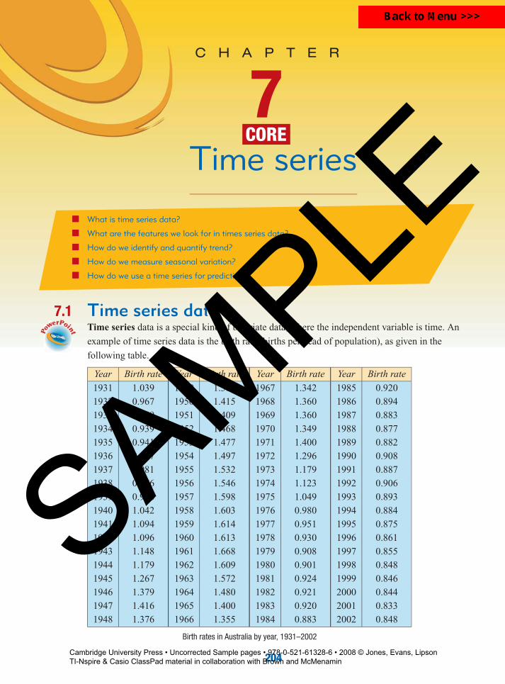
C H A P T E R 7 CORE Time series What is time series data? What are the features we look for in times series data? How do we identify and quantify trend? How do we measure seasonal variation? How do we use a time series for prediction? 7.1 Time series data Time series data is a special kind of bivariate data, where the independent variable is time. An example of time series data is the birth rate (births per head of population), as given in the following table. Year Birth rate Year Birth rate Year Birth rate Year Birth rate 1931 1.039 1949 1.382 1967 1.342 1985 0.920 1932 0.967 1950 1.415 1968 1.360 1986 0.894 1933 0.959 1951 1.409 1969 1.360 1987 0.883 1934 0.939 1952 1.468 1970 1.349 1988 0.877 1935 0.941 1953 1.477 1971 1.400 1989 0.882 1936 0.967 1954 1.497 1972 1.296 1990 0.908 1937 0.981 1955 1.532 1973 1.179 1991 0.887 1938 0.976 1956 1.546 1974 1.123 1992 0.906 1939 0.986 1957 1.598 1975 1.049 1993 0.893 1940 1.042 1958 1.603 1976 0.980 1994 0.884 1941 1.094 1959 1.614 1977 0.951 1995 0.875 1942 1.096 1960 1.613 1978 0.930 1996 0.861 1943 1.148 1961 1.668 1979 0.908 1997 0.855 1944 1.179 1962 1.609 1980 0.901 1998 0.848 1945 1.267 1963 1.572 1981 0.924 1999 0.846 1946 1.379 1964 1.480 1982 0.921 2000 0.844 1947 1.416 1965 1.400 1983 0.920 2001 0.833 1948 1.376 1966 1.355 1984 0.883 2002 0.848 Birth rates in Australia by year, 1931–2002 204 SAMPLE Cambridge University Press • Uncorrected Sample pages • 978-0-521-61328-6 • 2008 © Jones, Evans, Lipson TI-Nspire & Casio ClassPad material in collaboration with Brown and McMenamin

Welcome message from author
This document is posted to help you gain knowledge. Please leave a comment to let me know what you think about it! Share it to your friends and learn new things together.
Transcript
P1: FXS/ABE P2: FXS052160916Xc07-1.xml CUAU031-EVANS September 4, 2008 13:23
C H A P T E R
7CORE
Time series
What is time series data?
What are the features we look for in times series data?
How do we identify and quantify trend?
How do we measure seasonal variation?
How do we use a time series for prediction?
7.1 Time series dataTime series data is a special kind of bivariate data, where the independent variable is time. An
example of time series data is the birth rate (births per head of population), as given in the
following table.
Year Birth rate Year Birth rate Year Birth rate Year Birth rate
1931 1.039 1949 1.382 1967 1.342 1985 0.920
1932 0.967 1950 1.415 1968 1.360 1986 0.894
1933 0.959 1951 1.409 1969 1.360 1987 0.883
1934 0.939 1952 1.468 1970 1.349 1988 0.877
1935 0.941 1953 1.477 1971 1.400 1989 0.882
1936 0.967 1954 1.497 1972 1.296 1990 0.908
1937 0.981 1955 1.532 1973 1.179 1991 0.887
1938 0.976 1956 1.546 1974 1.123 1992 0.906
1939 0.986 1957 1.598 1975 1.049 1993 0.893
1940 1.042 1958 1.603 1976 0.980 1994 0.884
1941 1.094 1959 1.614 1977 0.951 1995 0.875
1942 1.096 1960 1.613 1978 0.930 1996 0.861
1943 1.148 1961 1.668 1979 0.908 1997 0.855
1944 1.179 1962 1.609 1980 0.901 1998 0.848
1945 1.267 1963 1.572 1981 0.924 1999 0.846
1946 1.379 1964 1.480 1982 0.921 2000 0.844
1947 1.416 1965 1.400 1983 0.920 2001 0.833
1948 1.376 1966 1.355 1984 0.883 2002 0.848
Birth rates in Australia by year, 1931–2002
204
SAMPLE
Cambridge University Press • Uncorrected Sample pages • 978-0-521-61328-6 • 2008 © Jones, Evans, Lipson TI-Nspire & Casio ClassPad material in collaboration with Brown and McMenamin

P1: FXS/ABE P2: FXS052160916Xc07-1.xml CUAU031-EVANS September 4, 2008 13:23
Chapter 7 — Time series 205
This data set is rather complex, and it is hard to see any patterns. However, as with other
forms of bivariate data, we will start to get an idea about the relationship between the variables
by drawing a scatterplot. When the scatterplot is a plot of time series data it is called a time
series plot, with time always placed on the horizontal axis. A time series plot differs from a
normal scatterplot in that the points will be joined by line segments in time order. A time series
plot of the birth rate data is given below.
1.8
1.6
1.4
1.2
1.0
0.8
1940 1960 1980 2000
Year
Bir
th r
ate
In general, a time series plot is a bivariate plot where the values of the dependent variable
are plotted in time order. Points in a time series plot are joined by line segments.
What are the features to look for in a time series plot? Time series data is often complex and
shows seemingly wild fluctuations. The fluctuations are generally due to one or more of the
following characteristics of the relationship:
trend
seasonal variation
cyclical variation
random variation
TrendWhen we examine a time series plot we are often able to discern a general upward or
downward movement over the long term, indicating a long-term change in the level of the
variable. This overall pattern is called the trend. One way of identifying trends on a time series
graph is to draw in a line that ignores the fluctuations but which reflects the overall increasing
or decreasing nature of the plot. These are called trend lines. Trend lines have been drawn in
on the time series plots below to indicate an increasing trend (line slopes upwards) and
decreasing trend (line slopes downwards).
Trend line
Time
Trend line
Time
Sometimes, as in the birth rate time series plot, different trends are apparent for different
parts of the plot. We can see this by drawing in trend lines on the plot.
SAMPLE
Cambridge University Press • Uncorrected Sample pages • 978-0-521-61328-6 • 2008 © Jones, Evans, Lipson TI-Nspire & Casio ClassPad material in collaboration with Brown and McMenamin

P1: FXS/ABE P2: FXS052160916Xc07-1.xml CUAU031-EVANS September 4, 2008 13:23
206 Essential Further Mathematics – Core
1.8
1.6
1.4
1.2
1.0
0.8
1940 1960 1980 2000Year
Bir
th r
ate
Trend 1Trend 2
Trend 3
Trend 1: From about 1940 to 1961 the birth rate grew quite dramatically. Those in the armed
services came home from the war, and the economy grew quickly. This rapid increase in
the birth rate is known as the Baby Boom.
Trend 2: From about 1962 until 1980 the birth rate declined very rapidly. Birth control
methods became more effective, and women started to think more about careers. This period
has sometimes been referred to as the Baby Bust.
Trend 3: During the 1980s and up until this time, the birth rate continues to decline slowly for
a complex range of social and economic reasons.
Seasonal variationSeasonal variations are repetitive fluctuating movements which occur within a time period of
one year or less. Seasonal movements tend to be more predictable than trends, and occur
because of the variation in weather, such as sales of ice-cream for instance, or institutional
factors, such as the increase in the number of unemployed at the end of the school year. The
plot below shows the total percentage of rooms occupied in hotels, motels, etc., in Australia by
quarter over the years 1998–2000.
The graph shows a general increasing trend, indicated by the upward sloping trend line. This
indicates that the demand for accommodation is increasing over time.
54
56
58
60
62
64
66
Roo
ms
(%)
Mar-
98
Jun-
98
Sep-9
8
Dec-9
8
Mar-
99
Jun-
99
Sep-9
9
Dec-9
9
Mar-
00
Jun-
00
Sep-0
0
Dec-0
0
However, over and above the general increasing trend, we can see that the demand for
accommodation also appears to be seasonal. The demand for accommodation is at its lowest in
the June quarter and peaks in the December quarter each year. Seasonality is identified by
looking for peaks and troughs at the same time each year.
SAMPLE
Cambridge University Press • Uncorrected Sample pages • 978-0-521-61328-6 • 2008 © Jones, Evans, Lipson TI-Nspire & Casio ClassPad material in collaboration with Brown and McMenamin

P1: FXS/ABE P2: FXS052160916Xc07-1.xml CUAU031-EVANS September 4, 2008 13:23
Chapter 7 — Time series 207
CyclesThe term cycle is used to describe longer term movements about the general trend line in the
time series which are not seasonal. Some cycles repeat regularly, and some do not. The
following plot shows the activity of sunspots, which are dark spots visible on the surface of the
sun. This shows a fairly regular cycle of approximately 11 years.
1900
1910
1920
1930
1940
1950
1960
1970
1980
1990
2000
2010
0
50
100
150
200
Year
Suns
pots
Many business indicators, such as interest rates or unemployment figures, also vary in
cycles, but their periods are usually less regular. In many contexts, including business,
movements are only considered cyclical if they occur in time intervals of more than one year.
Random variationRandom or irregular variation is the part of the time series which cannot be classified into one
of the above three categories. Generally, as with all variables, there can be many sources of
random variation. Sometimes a specific cause such as a war or a strike can be isolated as the
source of this variation. The aim of time series analysis is to develop techniques that can be
used to measure things such as trend and seasonality in time series, given that there will always
be random variation to cloud the picture.
Constructing time series plotsMost real-world time series data comes in the form of large data sets which are best plotted
with the aid of a spreadsheet or statistical package. The availability of the data in electronic
form via the web greatly helps the process. However, in this chapter, most of the time series
data sets are relatively small and can be plotted using a graphics calculator.
How to construct a time series plot using a graphics calculator
Construct a time series plot for the following data. The years have been recoded as
1, 2, . . . , 12, as is common practice.
1991 1992 1993 1994 1995 1996 1997 1998 1999 2000 2001 2002
1 2 3 4 5 6 7 8 9 10 11 12
0.887 0.906 0.893 0.884 0.875 0.861 0.855 0.848 0.846 0.844 0.833 0.848
Steps1 Enter the data into the calculator as shown (the calculator
mode has been set to 3 decimal places here).
SAMPLE
Cambridge University Press • Uncorrected Sample pages • 978-0-521-61328-6 • 2008 © Jones, Evans, Lipson TI-Nspire & Casio ClassPad material in collaboration with Brown and McMenamin

P1: FXS/ABE P2: FXS052160916Xc07-1.xml CUAU031-EVANS September 4, 2008 13:23
208 Essential Further Mathematics – Core
2 Select STATPLOT, turn the plot On. Move the cursor down
to Type: and then across to the times series plot icon Ó
as shown. Press b so that this plot is highlighted.
3 Move the cursor down to Xlist: and then use y94
to access the LIST menu. Press b to paste in the list
YEAR. Repeat to paste the list BIRTH against Ylist: as shown.
4 Press q® to obtain a time series plot for birth rates.
Exercise 7A
Throughout this chapter, use a graphics calculator whenever you wish
1 Complete a table like the one shown by indicating which of the listed characteristics are
present in each of the time series plots shown below.
Characteristic A B C
random variation
increasing trend
decreasing trend
cyclical variation
seasonal variation
0
10
5
15
20
25
30
35
40
1994 1995 1996 1997 1998 1999 2000Year
A
B
C
2 Complete the table by indicating which of the listed characteristics are present in each of the
time series plots shown below.
Characteristic A B C
random variation
increasing trend
decreasing trend
cyclical variation
seasonal variation
0
10
5
15
20
25
30
35
40
1994 1995 1996 1997 1998 1999 2000Year
A
B
C
SAMPLE
Cambridge University Press • Uncorrected Sample pages • 978-0-521-61328-6 • 2008 © Jones, Evans, Lipson TI-Nspire & Casio ClassPad material in collaboration with Brown and McMenamin
P1: FXS/ABE P2: FXS052160916Xc07-1.xml CUAU031-EVANS September 4, 2008 13:23
Chapter 7 — Time series 209
3 The time series plot opposite shows the
number of whales caught during the
period 1920–85. Describe the features
of the plot.
0
2010
30405060 70
1920
1930
1940
1950
1960
1970
1980
Year
Num
ber
of w
hale
s (0
00s)
4 The hotel room occupancy rate (%) in Victoria over the period March 1998–December 2000
is depicted below. Describe the features of the plot.
7472706866
646260
5856
Roo
ms
(%)
Mar-
98
Jun-
98
Sep-9
8
Dec-9
8
Mar-
99
Jun-
99
Sep-9
9
Dec-9
9
Mar-
00
Jun-
00
Sep-0
0
Dec-0
0
5 The time series plot below shows the smoking rates (%) of Australian males and females
who smoked over the period 1945–92.
a Describe any trends in the time series plot.
b Did the difference in smoking rates increase
or decrease over the period 1945 to 1992?
20
10
30
40
50
60
70
80
1945 1955 1965
Females
Males
1975 1985 1995
Year
Smok
ers
(per
cent
age)
0
6 Use the data below to construct a time series plot of the birth rate in Australia for 1960–70.
Year 1960 1961 1962 1963 1964 1965 1966 1967 1968 1969 1970
Rate 1.613 1.668 1.609 1.572 1.480 1.400 1.355 1.342 1.360 1.360 1.349
7 Use the data below to construct a time series plot of the population (in millions) in Australia
over the period 1993–2003.
Year 1993 1994 1995 1996 1997 1998 1999 2000 2001 2002 2003
Population 17.8 18.0 18.2 18.4 18.6 18.8 19.0 19.3 19.5 19.8 20.0
SAMPLE
Cambridge University Press • Uncorrected Sample pages • 978-0-521-61328-6 • 2008 © Jones, Evans, Lipson TI-Nspire & Casio ClassPad material in collaboration with Brown and McMenamin

P1: FXS/ABE P2: FXS052160916Xc07-1.xml CUAU031-EVANS September 4, 2008 13:23
210 Essential Further Mathematics – Core
8 Use the data below to construct a time series plot for the number of school teachers (in
thousands) in Australia over the period 1993–2001.
Year 1991 1992 1993 1994 1995 1996 1997 1998 1999 2000 2001
Teachers 213 217 218 218 221 223 228 231 239 244 250
9 The table below gives the number of male and female teachers (in thousands) in Australia
over the years 1993 to 2001.
Year 1993 1994 1995 1996 1997 1998 1999 2000 2001
Males ’000 77.9 76.6 75.3 75.0 74.9 74.9 76.0 76.6 77.1
Females ’000 139.9 141.2 145.5 148.5 152.5 156.0 163.4 167.4 172.5
a Construct a time series plot that shows both the male and female data on the same graph.
b Describe and comment on any trends you observe.
7.2 Smoothing a time series plot (moving means)A time series plot can incorporate many of the sources of variation previously mentioned:
trend, seasonality, cycles and random variation.
Because of the local variation, it is sometimes difficult to see the overall pattern. In order to
clarify the situation, a technique known as smoothing may be helpful. Smoothing can be used
to enhance and emphasise any trend in the data by eliminating the noisy jagged components,
and allowing us to construct a line (possibly curved) that exhibits the trend of the times series.
We shall discuss two of the most common smoothing methods, moving mean and moving
median.
Moving mean smoothingThis method of smoothing involves the computation of moving means. The simplest method
is to smooth over odd numbers of points, for example, 3, 5, 7.
The 3-moving meanTo use 3-moving mean smoothing, replace each data value with the mean of that value and
the values of its two neighbours, one on each side. That is, if y1, y2 and y3 are sequential
data values then:
smoothed y2 = y1 + y2 + y3
3
The first and last points do not have values on each side, so they are omitted.
For example, for the values shown in the table below:
Year 1 2 3
y 9 11 10(y1) (y2) (y3)
smoothed y2 = y1 + y2 + y3
3
= 9 + 11 + 10
3= 10
SAMPLE
Cambridge University Press • Uncorrected Sample pages • 978-0-521-61328-6 • 2008 © Jones, Evans, Lipson TI-Nspire & Casio ClassPad material in collaboration with Brown and McMenamin

P1: FXS/ABE P2: FXS052160916Xc07-1.xml CUAU031-EVANS September 4, 2008 13:23
Chapter 7 — Time series 211
Similarly:
The 5-moving meanTo use 5-moving mean smoothing, replace each data value with the mean of that value and
the two values on each side. That is, if y1, y2, y3, y4, y5, are sequential data values then:
smoothed y3 = y1 + y2 + y3 + y4 + y5
5
The first two and last two points do not have two values on each side, so they are omitted.
For example, for the values shown in the table below:
Year 1 2 3 4 5
y 9 11 10 12 13(y1) (y2) (y3) (y4) (y5)
smoothed y3 = y1 + y2 + y3 + y4 + y5
5
= 9 + 11 + 10 + 12 + 13
5= 11
These definitions can readily be extended for smoothing over 7, 9, 11, etc, points. The larger
the number of points we smooth over, the greater the smoothing effect.
Example 1 3- and 5-moving mean smoothing
The following table gives the number of births per month over a calendar year in a small
country hospital. Use the 3-moving mean and the 5-moving mean methods, correct to one
decimal place, to complete the table.
Solution
Month Number of births 3-moving mean 5-moving mean
January 10
February 1210 + 12 + 6
March 61 2 + 6 + 5 = 7.7
10 + 12 + 6 + 5 + 22
April 56 + 5 + 22 = 11.0 12+6 + 5 + 22 + 18
May 225 +2 2 +1 8 6 + 5 + 22 + 18 + 13 = 12.8
June 18 22 + 18 + 13 5 + 22 + 18 + 13 + 7 = 13.0
July 1318 + 13 + 7 2 2 + 18 + 13 + 7 + 9 = 13.8
August 713 + 7 + 9 1 8 + 13 + 7 + 9 + 10 = 11.4
September 97 + 9 + 10 1 3 + 7 + 9 + 10 + 8 = 9.4
October 109 + 10 + 8 7 + 9 + 10 + 8 + 15 = 9.8
November 810 + 8 + 15
December 15
3 5
5
5
5
5
5
5
5
3
3
3
3
3
3
3
3
3= 9.3
= 15.0
= 17.7
= 12.7
= 9.7
= 8.7
= 9.0
= 11.0
= 11.0
= 12.6
SAMPLE
Cambridge University Press • Uncorrected Sample pages • 978-0-521-61328-6 • 2008 © Jones, Evans, Lipson TI-Nspire & Casio ClassPad material in collaboration with Brown and McMenamin
P1: FXS/ABE P2: FXS052160916Xc07-1.xml CUAU031-EVANS September 4, 2008 13:23
212 Essential Further Mathematics – Core
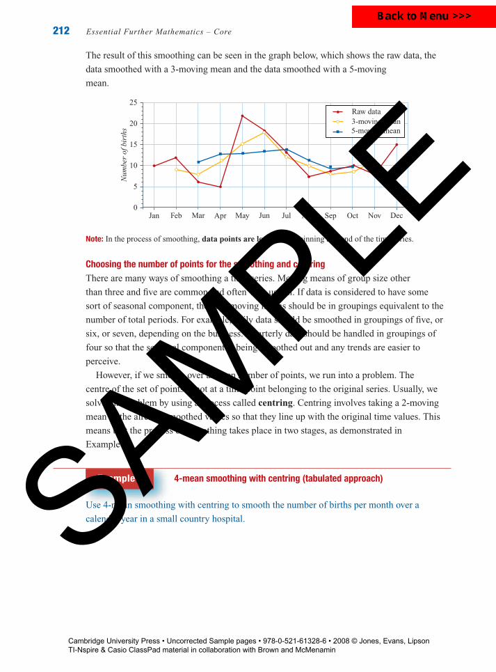
The result of this smoothing can be seen in the graph below, which shows the raw data, the
data smoothed with a 3-moving mean and the data smoothed with a 5-moving
mean.
Jan DecNovOctSepAugJulJunMayAprMarFeb0
10
5
15
20
25
Num
ber
of b
irth
sRaw data 3-moving mean5-moving mean
Note: In the process of smoothing, data points are lost at the beginning and end of the time series.
Choosing the number of points for the smoothing and centringThere are many ways of smoothing a time series. Moving means of group size other
than three and five are common and often very useful. If data is considered to have some
sort of seasonal component, then the moving means should be in groupings equivalent to the
number of total periods. For example, daily data should be smoothed in groupings of five, or
six, or seven, depending on the business. Quarterly data should be handled in groupings of
four so that the seasonal component is being smoothed out and any trends are easier to
perceive.
However, if we smooth over an even number of points, we run into a problem. The
centre of the set of points is not at a time point belonging to the original series. Usually, we
solve this problem by using a process called centring. Centring involves taking a 2-moving
mean of the already smoothed values so that they line up with the original time values. This
means that the process of smoothing takes place in two stages, as demonstrated in
Example 2.
Example 2 4-mean smoothing with centring (tabulated approach)
Use 4-mean smoothing with centring to smooth the number of births per month over a
calendar year in a small country hospital.SAMPLE
Cambridge University Press • Uncorrected Sample pages • 978-0-521-61328-6 • 2008 © Jones, Evans, Lipson TI-Nspire & Casio ClassPad material in collaboration with Brown and McMenamin

P1: FXS/ABE P2: FXS052160916Xc07-1.xml CUAU031-EVANS September 4, 2008 13:23
Chapter 7 — Time series 213
Solution
4-moving mean with
Month Number of births 4-moving mean centring
January 10
February 1210 + 12 + 6 + 5
4= 8.25
March 68.25 + 11.25
2= 9.75
12 + 6 + 5 + 22
4= 11.25
April 511.25 + 12.75
2= 12
6 + 5 + 22 + 18
4= 12.75
May 2212.75 + 14.5
2= 13.625
5 + 22 + 18 + 13
4= 14.5
June 1814.5 + 15
2= 14.75
22 + 18 + 13 + 7
4= 15
July 1315 + 11.75
2= 13.375
18 + 13 + 7 + 9
4= 11.75
August 711.75 + 9.75
2= 10.75
13 + 7 + 9 + 10
4= 9.75
September 99.75 + 8.5
2= 9.125
7 + 9 + 10 + 8
4= 8.5
October 108.5 + 10.5
2= 9.5
9 + 10 + 8 + 15
4= 10.5
November 8
December 15SAMPLE
Cambridge University Press • Uncorrected Sample pages • 978-0-521-61328-6 • 2008 © Jones, Evans, Lipson TI-Nspire & Casio ClassPad material in collaboration with Brown and McMenamin
P1: FXS/ABE P2: FXS052160916Xc07-1.xml CUAU031-EVANS September 4, 2008 13:23
214 Essential Further Mathematics – Core
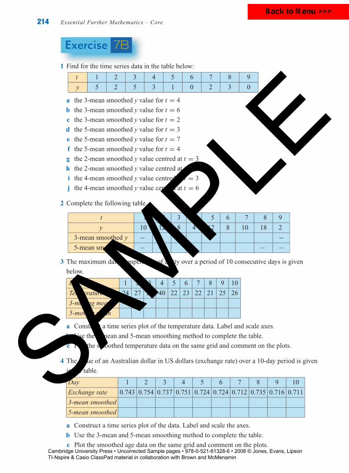
Exercise 7B
1 Find for the time series data in the table below:
t 1 2 3 4 5 6 7 8 9
y 5 2 5 3 1 0 2 3 0
a the 3-mean smoothed y value for t = 4
b the 3-mean smoothed y value for t = 6
c the 3-mean smoothed y value for t = 2
d the 5-mean smoothed y value for t = 3
e the 5-mean smoothed y value for t = 7
f the 5-mean smoothed y value for t = 4
g the 2-mean smoothed y value centred at t = 3
h the 2-mean smoothed y value centred at t = 8
i the 4-mean smoothed y value centred at t = 3
j the 4-mean smoothed y value centred at t = 6
2 Complete the following table.
t 1 2 3 4 5 6 7 8 9
y 10 12 8 4 12 8 10 18 2
3-mean smoothed y − −5-mean smoothed y − − − −
3 The maximum daily temperature of a city over a period of 10 consecutive days is given
below.
Day 1 2 3 4 5 6 7 8 9 10
Temperature (◦C) 24 27 28 40 22 23 22 21 25 26
3-moving mean
5-moving mean
a Construct a time series plot of the temperature data. Label and scale axes.
b Use the 3-mean and 5-mean smoothing method to complete the table.
c Plot the smoothed temperature data on the same grid and comment on the plots.
4 The value of an Australian dollar in US dollars (exchange rate) over a 10-day period is given
in the table.
Day 1 2 3 4 5 6 7 8 9 10
Exchange rate 0.743 0.754 0.737 0.751 0.724 0.724 0.712 0.735 0.716 0.711
3-mean smoothed
5-mean smoothed
a Construct a time series plot of the data. Label and scale the axes.
b Use the 3-mean and 5-mean smoothing method to complete the table.
c Plot the smoothed age data on the same grid and comment on the plots.
SAMPLE
Cambridge University Press • Uncorrected Sample pages • 978-0-521-61328-6 • 2008 © Jones, Evans, Lipson TI-Nspire & Casio ClassPad material in collaboration with Brown and McMenamin

P1: FXS/ABE P2: FXS052160916Xc07-1.xml CUAU031-EVANS September 4, 2008 13:23
Chapter 7 — Time series 215
5 Complete the following table by using 2-mean smoothing with centring.
Month Number of births 2-moving 2-moving meanmean with centring
January 10February 12March 6April 5May 22June 18July 13August 7September 9October 10November 8December 15
6 The data in the table shows internet usage (in gigabytes of information downloaded) at a
university from April to December. Complete the table by using 2-mean smoothing with
centring.
Month Internet usage 2-moving 2-moving meanmean with centring
April 21
May 40
June 52
July 42
August 58
September 79
October 81
November 54
December 50
7.3 Smoothing a time series plot (moving medians)Median smoothingAnother simple and convenient way of smoothing the times series is to use moving medians.
The advantage of the moving median technique is that it is:
primarily a graphical technique (although it can be done numerically) that enables the
smoothed time series to be constructed directly from the original time series plot
not influenced by a single outlier, thus any unusual values will be eliminated very
quickly
SAMPLE
Cambridge University Press • Uncorrected Sample pages • 978-0-521-61328-6 • 2008 © Jones, Evans, Lipson TI-Nspire & Casio ClassPad material in collaboration with Brown and McMenamin

P1: FXS/ABE P2: FXS052160916Xc07-1.xml CUAU031-EVANS September 4, 2008 13:23
216 Essential Further Mathematics – Core
The 3-moving medianTo use 3-moving median smoothing, replace each data value with the median of that value
and the values of its two neighbours, one on each side. That is, if y1, y2 and y3 are sequential
data values then:
smoothed y2 = median (y1, y2, y3)
The first and last points do not have values on each side, so they are omitted.
For example, for the values shown in the table below:
Year 1 2 3
(y) 9 11 10(y1) (y2) (y3)
smoothed y2 is the median of: 9, 11, 10
9, 10, 11
∴ smoothed y2 = 10
Similarly:
The 5-moving medianTo use 5-moving median smoothing, replace each data value with the median of that value
and the two values on each side. That is, if y1, y2, y3, y4, y5, are sequential data values then:
smoothed y3 = median (y1, y2, y3, y4, y5)
The first two and last two points do not have two values on each side, so they are omitted.
For example, for the values shown in the table below:
Year 1 2 3 4 5
y 9 11 10 12 13(y1) (y2) (y3) (y4) (y5)
smoothed y3 is the median of: 9, 11, 10, 12, 13
9, 10, 11©, 12, 13
∴ smoothed y3 = 11
This definition can readily be extended for smoothing over 7, 9, 11, etc. points.
Example 3 3- and 5-median smoothing
The following table gives the number of births per month over a calendar year in a small
country hospital. Use the 3-moving median and the 5-moving median methods, correct to one
decimal place, to complete the table.
Solution
Month Number of births 3-moving median 5-moving median
January 10
February 12 M edi an = 10March 6 M edi an = 6 M edi an = 10April 5 6 12May 22 18 13June 18 18 13July 13 13 13August 7 9 9September 9 9 9October 10 9November 8 10December 15
SAMPLE
Cambridge University Press • Uncorrected Sample pages • 978-0-521-61328-6 • 2008 © Jones, Evans, Lipson TI-Nspire & Casio ClassPad material in collaboration with Brown and McMenamin
P1: FXS/ABE P2: FXS052160916Xc07-1.xml CUAU031-EVANS September 4, 2008 13:23
Chapter 7 — Time series 217
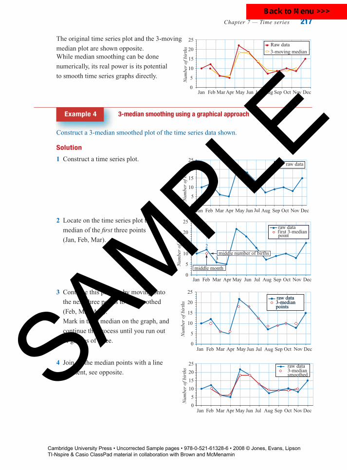
The original time series plot and the 3-moving
median plot are shown opposite.
0
10
5
15
20
25
Num
ber
of b
irth
s Raw data 3-moving median
Jan Feb Mar Apr May Jun Jul Aug Sep Oct Nov Dec
While median smoothing can be done
numerically, its real power is its potential
to smooth time series graphs directly.
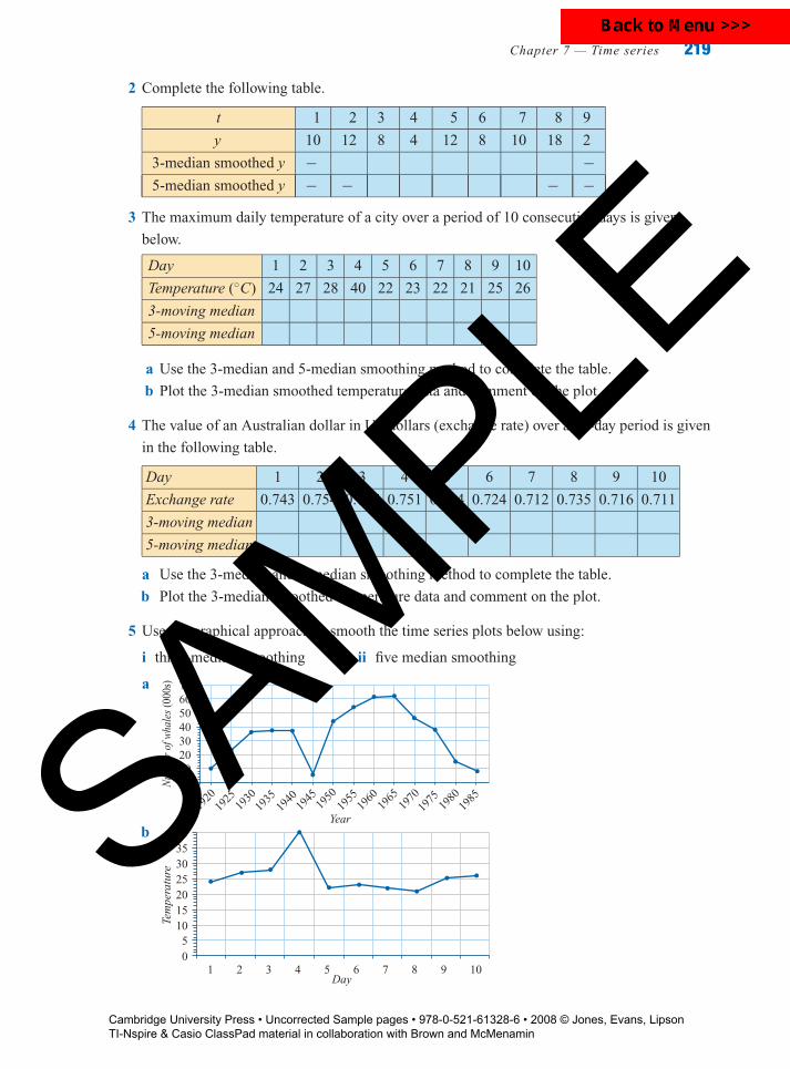
Example 4 3-median smoothing using a graphical approach
Construct a 3-median smoothed plot of the time series data shown.
Solution
1 Construct a time series plot.
0
5
10
15
20
25
Num
ber
of b
irth
s raw data
Jan Feb Mar Apr May Jun Jul Aug Sep Oct Nov Dec
2 Locate on the time series plot the
median of the first three points
(Jan, Feb, Mar).
0
5
10
15
20
25
Num
ber
of b
irth
s
12
3
raw datafirst 3-medianpoint
middle month
middle number of births
Jan Feb Mar Apr May Jun Jul Aug Sep Oct Nov Dec
3 Continue this process by moving onto
the next three points to be smoothed
(Feb, Mar, Apr).
Mark in their median on the graph, and
continue the process until you run out
of groups of three. 0
5
10
15
20
25
Num
ber
of b
irth
s
raw dataraw data3-median3-medianpointspoints
Jan Feb Mar Apr May Jun Jul Aug Sep Oct Nov Dec
4 Join up the median points with a line
segment, see opposite.
0
5
10
15
20
25
Num
ber
of b
irth
s raw data3-mediansmoothed
Jan Feb Mar Apr May Jun Jul Aug Sep Oct Nov Dec
SAMPLE
Cambridge University Press • Uncorrected Sample pages • 978-0-521-61328-6 • 2008 © Jones, Evans, Lipson TI-Nspire & Casio ClassPad material in collaboration with Brown and McMenamin

P1: FXS/ABE P2: FXS052160916Xc07-2.xml CUAU031-EVANS September 4, 2008 13:31
218 Essential Further Mathematics – Core
Example 5 5-median smoothing using a graphical approach
Construct a 5-median smoothed plot of the time series data shown.
Solution
1 Locate on the time series plot the median of
the first five points (Jan, Feb, Mar, Apr, May)
as shown opposite.
0
5
10
15
20
25
Num
ber
of b
irth
s
Jan
Feb
Mar
AprM
ay Jun
Jul
Aug Sep OctNov Dec
raw datafirst 5-medianpoint
middle number of births
middle month
12
3 4
5
2 Then move onto the next five points to be
smoothed (Feb, Mar, Apr, May, Jun) The
process is then repeated until you run out
of groups of five points. The 5-median
points are then joined up with line segments
to give the final smoothed plot as shown. 0
5
10
15
20
25
Num
ber
of b
irth
sJa
nFe
bM
arApr
May Ju
nJu
lAug Sep Oct
Nov Dec
raw data5-mediansmoothed
Note: The five-median smoothed plot is much smoother than the three-median smoothed plot.
When smoothing is carried out over an even number of data points, centring is again used to
align the smoothed values with the original time periods.
Exercise 7C
1 Find for the time series data in the table:
t 1 2 3 4 5 6 7 8 9
y 5 2 5 3 1 0 2 3 0
a the 3-median smoothed y value for t = 4
b the 3-median smoothed y value for t = 6
c the 3-median smoothed y value for t = 2
d the 5-median smoothed y value for t = 3
e the 5-median smoothed y value for t = 7
f the 5-median smoothed y value for t = 4
g the 2-median smoothed y value centred at t = 3
h the 2-median smoothed y value centred at t = 8
i the 4-median smoothed y value centred at t = 3
j the 4-median smoothed y value centred at t = 6
SAMPLE
Cambridge University Press • Uncorrected Sample pages • 978-0-521-61328-6 • 2008 © Jones, Evans, Lipson TI-Nspire & Casio ClassPad material in collaboration with Brown and McMenamin
P1: FXS/ABE P2: FXS052160916Xc07-2.xml CUAU031-EVANS September 4, 2008 13:31
Chapter 7 — Time series 219
2 Complete the following table.
t 1 2 3 4 5 6 7 8 9
y 10 12 8 4 12 8 10 18 2
3-median smoothed y − −5-median smoothed y − − − −
3 The maximum daily temperature of a city over a period of 10 consecutive days is given
below.
Day 1 2 3 4 5 6 7 8 9 10
Temperature (◦C) 24 27 28 40 22 23 22 21 25 26
3-moving median
5-moving median
a Use the 3-median and 5-median smoothing method to complete the table.
b Plot the 3-median smoothed temperature data and comment on the plot.
4 The value of an Australian dollar in US dollars (exchange rate) over a 10-day period is given
in the following table.
Day 1 2 3 4 5 6 7 8 9 10
Exchange rate 0.743 0.754 0.737 0.751 0.724 0.724 0.712 0.735 0.716 0.711
3-moving median
5-moving median
a Use the 3-median and 5-median smoothing method to complete the table.
b Plot the 3-median smoothed temperature data and comment on the plot.
5 Use the graphical approach to smooth the time series plots below using:
i three-median smoothing ii five median smoothing
a
010203040506070
Num
ber
of w
hale
s (0
00s)
Year19
2019
2519
3019
3519
4019
4519
5019
5519
6019
6519
7019
7519
8019
85
b
1 2 3 4 5 6 7 8 9 10Day
Tem
pera
ture
05
10152025303540SAM
PLE
Cambridge University Press • Uncorrected Sample pages • 978-0-521-61328-6 • 2008 © Jones, Evans, Lipson TI-Nspire & Casio ClassPad material in collaboration with Brown and McMenamin

P1: FXS/ABE P2: FXS052160916Xc07-2.xml CUAU031-EVANS September 4, 2008 13:31
220 Essential Further Mathematics – Core
6 The time series plot below shows the percentage growth of GDP (gross domestic product)
over a 13-year period.
1 2 3 4 5 6 7 8 9 12
Gro
wth
in G
DP
(%
)
–2
–1
0
1
2
3
4
5
6
10 11 13
a Smooth the times series graph:
i using 3-median smoothing ii using 5-median smoothing
b What conclusions can be drawn about the variation in GDP growth from these time series
plots?
7.4 Seasonal indicesWhen the data under consideration has a seasonal component, it is often necessary to remove
this component by deseasonalising the data before further analysis. To do this we need to
calculate seasonal indices. Seasonal indices tell us how a particular season (generally a day,
month or quarter) compares to the average season.
Consider the (hypothetical) monthly seasonal indices for unemployment given in the table
below:
Jan Feb Mar Apr May Jun Jul Aug Sept Oct Nov Dec Total
1.1 1.2 1.1 1.0 0.95 0.95 0.9 0.9 0.85 0.85 1.1 1.1 12.0
Seasonal indices are calculated so that their average is 1. This means that the sum of the
seasonal indices equals the number of seasons. Thus, if the seasons are months, the seasonal
indices add to 12. If the seasons are quarters, then the seasonal indices would add to 4, and so
on.
Interpreting seasonal indicesThe seasonal index for unemployment for the month of February is 1.2.
Seasonal indices are easier to interpret if we convert them to percentages. Remember, to
convert a number to a percentage, just multiply by 100.
A seasonal index of 1.2 for February, written in percentage terms, is 120%.
A seasonal index of 1.2 (or 120%) tells us that February unemployment figures tend to be
20% higher than the monthly average. Remember, the average seasonal index is 1 or
100%.
The seasonal index for August is 0.90 or 90%.
A seasonal index of 0.9 (or 90%) tells us that the August unemployment figures tend to be
only 90% of the monthly average. Alternatively, August unemployment figures are 10%
lower than the monthly average.
SAMPLE
Cambridge University Press • Uncorrected Sample pages • 978-0-521-61328-6 • 2008 © Jones, Evans, Lipson TI-Nspire & Casio ClassPad material in collaboration with Brown and McMenamin

P1: FXS/ABE P2: FXS052160916Xc07-2.xml CUAU031-EVANS September 4, 2008 13:31
Chapter 7 — Time series 221
The seasonal indexA season index is defined by the formula:
seasonal index = value for season
seasonal average
In this formula, the season is a month, quarter or the like. The seasonal average is the
monthly average, the quarterly average, and so on.
Seasonal indices have the property that the sum of the seasonal indices equals the
number of seasons.
Example 6 Calculating seasonal indices (one year’s data)
Mikki runs a shop and she wishes to
determine quarterly seasonal indices
based on her last year’s sales,
which are shown in the table opposite.
Summer Autumn Winter Spring
920 1085 1241 446
Solution
1 The seasonal index is defined by:
seasonal index = value for season
seasonal average
The seasons are quarters. Write
the formula in terms of quarters.
2 Find the quarterly average for
the year.
3 Work out the seasonal index
(SI) for each time period.
seasonal index = value for quarter
quarterly average
quarterly average = 920 + 1085 + 1241 + 446
4
= 923
SISummer
= 920
923= 0.997
SIAutumn
= 1085
923= 1.176
SIWinter
= 1241
923= 1.345
SISpring
= 446
923= 0.483
4 Check that the seasonal indices
sum to 4 (the number of seasons).
The slight difference here is due to
rounding error.
5 Write out your answers as a
table of the seasonal indices.
Check: 0.997 + 1.176 + 1.345 + 0.483 = 4.001
Seasonal indices
Summer Autumn Winter Spring
0.997 1.176 1.345 0.483
SAMPLE
Cambridge University Press • Uncorrected Sample pages • 978-0-521-61328-6 • 2008 © Jones, Evans, Lipson TI-Nspire & Casio ClassPad material in collaboration with Brown and McMenamin

P1: FXS/ABE P2: FXS052160916Xc07-2.xml CUAU031-EVANS September 4, 2008 13:31
222 Essential Further Mathematics – Core
Mikki actually has three previous year’s data to work with and the time series plot confirms her
belief that her sales are seasonal. The first quarter in the period has been labelled Quarter 1,
and then each quarter labelled consecutively.
1 2 3 4 5 6 7 8 9 10 11 12
600
1200Sa
les
Quarter
The next example illustrates how seasonal indices are calculated with several years’ data.
While the process looks more complicated, we just repeat what we did in Example 6 three
times and average the results for each year at the end.
Example 7 Calculating seasonal indices (several years’ data)
Suppose that Mikki has in fact three years of data, as shown. Use this data to calculate seasonal
indices, correct to two decimal places.
Year Summer Autumn Winter Spring
1 920 1085 1241 446
2 1035 1180 1356 541
3 1299 1324 1450 659
Solution
The strategy is as follows:� calculate the seasonal indices for Years 1, 2 and 3 separately as for Example 6 (as we
already have the seasonal indices for Year 1 from Example 6 we will save ourselves some
time by simply quoting the result)� average the three sets of seasonal indices at the end to obtain a single set of seasonal indices
1 Write down the result for Year 1.
2 Now calculate the seasonal indices
for Year 2.
Year 1 seasonal indices:
Summer Autumn Winter Spring
0.997 1.176 1.345 0.483
Year 2 seasonal indices:
3 The seasonal index is defined by:
seasonal index = value for season
seasonal average
The seasons are quarters. Write
the formula in terms of quarters.
seasonal index = value for quarter
quarterly averageSAMPLE
Cambridge University Press • Uncorrected Sample pages • 978-0-521-61328-6 • 2008 © Jones, Evans, Lipson TI-Nspire & Casio ClassPad material in collaboration with Brown and McMenamin

P1: FXS/ABE P2: FXS052160916Xc07-2.xml CUAU031-EVANS September 4, 2008 13:31
Chapter 7 — Time series 223
4 Find the quarterly average for
the year.Quart. average = 1035 + 1180 + 1356 + 541
4
= 1028
5 Work out the seasonal index (SI)
for each time period.
6 Check that the seasonal indices
sum to 4 (the number of seasons).
7 Write out your answers as a table
of the seasonal indices.
8 Now calculate the seasonal indices
for Year 3.
9 Find the quarterly average for
the year.
10 Work out the seasonal index
(SI) for each time period.
11 Check that the seasonal indices
sum to 4 (the number of seasons).
12 Write out your answers as a table
of the seasonal indices.
SISummer
= 1035
1028= 1.007
SIAutumn
= 1180
1028= 1.148
SIWinter
= 1356
1028= 1.319
SISpring
= 541
1028= 0.526
Check: 1.007 + 1.148 + 1.319 + 0.526 = 4.000
Summer Autumn Winter Spring
1.007 1.148 1.319 0.526
Year 3 seasonal indices:
Quart. average =1299 + 1324 + 1450 + 659
4= 1183
SISummer
= 1299
1183= 1.098
SIAutumn
= 1324
1183= 1.119
SIWinter
= 1450
1183= 1.226
SISpring
= 659
1183= 0.557
Check: 1.098 + 1.119 + 1.226 + 0.557 = 4.000
Summer Autumn Winter Spring
1.098 1.119 1.226 0.557
13 Find the 3-year averaged seasonal
indices by averaging the seasonal
indices for each season.
Final seasonal indices:
SSummer
= 0.997 + 1.007 + 1.098
3= 1.03
SAutumn
= 1.176 + 1.148 + 1.119
3= 1.15
SWinter
= 1.345 + 1.319 + 1.226
3= 1.30
SSpring
= 0.483 + 0.526 + 0.557
3= 0.52
SAMPLE
Cambridge University Press • Uncorrected Sample pages • 978-0-521-61328-6 • 2008 © Jones, Evans, Lipson TI-Nspire & Casio ClassPad material in collaboration with Brown and McMenamin

P1: FXS/ABE P2: FXS052160916Xc07-2.xml CUAU031-EVANS September 4, 2008 13:31
224 Essential Further Mathematics – Core
14 Check that the seasonal indices
sum to 4 (the number of seasons).
15 Write out your answers as a table
of the seasonal indices.
Check: 1.03 + 1.15 + 1.30 + 0.52 = 4.00
Summer Autumn Winter Spring
1.03 1.15 1.30 0.52
Having calculated these seasonal indices, what do they tell us?
A seasonal index of:1.03 for summer tells us that sales in summer are typically 3% above average
1.15 for autumn tells us that sales in autumn are typically 15% above average
1.30 for winter tells us that sales in winter are typically 30% above average
0.52 for spring tells us that sales in spring are typically 48% below average
Using seasonal indices to deseasonalise the dataWe can use seasonal indices to remove the seasonal component (deseasonalise) of a time series.
To calculate deseasonalised figures, each entry is divided by its seasonal index as follows.
Deseasonalising dataTime series data is deseasonalised using the relationship:
deseasonalised figure = actual figure
seasonal index
The resulting data can then be examined for long-term trends.
Example 8 Deseasonalising data
The quarterly sales figures for Mikki’s shop over a three-year period are given below.
Year Summer Autumn Winter Spring
1 920 1085 1241 446
2 1035 1180 1356 541
3 1299 1324 1450 659
Use the seasonal indices shown to
deseasonalise these sales figures giving
answers correct to the nearest whole number.
Summer Autumn Winter Spring
1.03 1.15 1.30 0.52
Solution
1 deseasonalised figure = actual figure
seasonal indexSummer
920
1.03= 893
1035
1.03= 1005
1299
103= 1261
2 To deseasonalise each sales figure in the
table, divide by the appropriate seasonal
index. For example, divide the figures in the
summer column by 1.03. Round results to the
nearest whole number.
SAMPLE
Cambridge University Press • Uncorrected Sample pages • 978-0-521-61328-6 • 2008 © Jones, Evans, Lipson TI-Nspire & Casio ClassPad material in collaboration with Brown and McMenamin
P1: FXS/ABE P2: FXS052160916Xc07-2.xml CUAU031-EVANS September 4, 2008 13:31
Chapter 7 — Time series 225
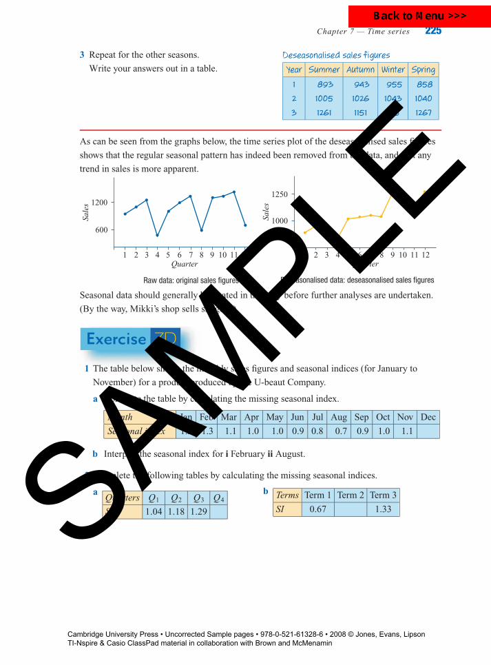
3 Repeat for the other seasons.
Write your answers out in a table.
Deseasonalised sales figures
Year Summer Autumn Winter Spring
1 893 943 955 858
2 1005 1026 1043 1040
3 1261 1151 1115 1267
As can be seen from the graphs below, the time series plot of the deseasonalised sales figures
shows that the regular seasonal pattern has indeed been removed from the data, and that any
trend in sales is more apparent.
1 2 3 4 5 6 7 8 9 10 11 12
600
1200
Sale
s
Quarter
Raw data: original sales figures
1 2 3 4 5 6 7 8 9 10 11 12
1000
1250
QuarterSa
les
Deseasonalised data: deseasonalised sales figures
Seasonal data should generally be treated in this way before further analyses are undertaken.
(By the way, Mikki’s shop sells ski gear.)
Exercise 7D
1 The table below shows the monthly sales figures and seasonal indices (for January to
November) for a product produced by the U-beaut Company.
a Complete the table by calculating the missing seasonal index.
Month Jan Feb Mar Apr May Jun Jul Aug Sep Oct Nov Dec
Seasonal index 1.2 1.3 1.1 1.0 1.0 0.9 0.8 0.7 0.9 1.0 1.1
b Interpret the seasonal index for i February ii August.
2 Complete the following tables by calculating the missing seasonal indices.
aQuarters Q1 Q2 Q3 Q4
SI 1.04 1.18 1.29
b Terms Term 1 Term 2 Term 3
SI 0.67 1.33SAMPLE
Cambridge University Press • Uncorrected Sample pages • 978-0-521-61328-6 • 2008 © Jones, Evans, Lipson TI-Nspire & Casio ClassPad material in collaboration with Brown and McMenamin

P1: FXS/ABE P2: FXS052160916Xc07-2.xml CUAU031-EVANS September 4, 2008 13:31
226 Essential Further Mathematics – Core
3 The table below shows the quarterly newspaper sales of a corner store for Year 1. Also
shown are the seasonal indices for newspaper sales for the first, second and third quarters.
Complete the table.
Quarter 1 Quarter 2 Quarter 3 Quarter 4
Year 1 1256 1060 1868 1642
Year 1 deseasonalised
Seasonal index 0.8 0.7 1.3
4 The quarterly cream sales (in litres) made by the same corner store in Year 1, along with
seasonal indices for cream sales for three of the four quarters, are shown in the table below.
Complete the table.
Quarter 1 Quarter 2 Quarter 3 Quarter 4
Year 1 68 102 115 84
Year 1 deseasonalised
Seasonal index 1.10 1.15 0.90
5 Each of the following data sets records quarterly sales ($000s). Use the data to determine
the seasonal indices for the four quarters. Give your results correct to two decimal places.
Check that your seasonal indices add to 4.
aQ1 Q2 Q3 Q4
48 41 60 65
bQ1 Q2 Q3 Q4
60 56 75 78
6 Each of the following data sets records monthly sales ($000s). Use the data to determine
the seasonal indices for the 12 months. Give your results correct to two decimal places.
Check that your seasonal indices add to 12.
a Jan Feb Mar Apr May Jun Jul Aug Sep Oct Nov Dec
12 13 14 17 18 15 9 10 8 11 15 20
b Jan Feb Mar Apr May Jun Jul Aug Sep Oct Nov Dec
22 19 25 23 20 18 20 15 14 11 23 30
7 The number of waiters employed by a restaurant chain in each quarter of one year, along
with some seasonal indices which have been calculated from the previous year’s data, are
given in the following table.
Quarter 1 Quarter 2 Quarter 3 Quarter 4
Number of waiters 198 145 86 168
Seasonal index 1.30 0.58 1.10
a What is the seasonal index for the second quarter?
b The seasonal index for Quarter 1 is 1.30. Explain what this mean in terms of the average
quarterly number of waiters.
c Deseasonalise the data.
8 The following table shows the number of students enrolled in a 3-month computer systems
training course along with some seasonal indices which have been calculated from the
previous year’s enrolment figures. Complete the table by calculating the seasonal index for
spring and the deseasonalised student numbers for each course.
SAMPLE
Cambridge University Press • Uncorrected Sample pages • 978-0-521-61328-6 • 2008 © Jones, Evans, Lipson TI-Nspire & Casio ClassPad material in collaboration with Brown and McMenamin

P1: FXS/ABE P2: FXS052160916Xc07-2.xml CUAU031-EVANS September 4, 2008 13:31
Chapter 7 — Time series 227
Summer Autumn Winter Spring
Number of students 56 125 126 96
Deseasonalised numbers
Seasonal index 0.5 1.0 1.3
9 The following table shows the monthly sales figures and seasonal indices (for January to
December) for a product produced by the VMAX company.
a Complete the table by:
i calculating the missing seasonal index
ii evaluating the deseasonalised sales figures
b The seasonal index for July is 0.90. Explain what this means in terms of the average
monthly sales.
Jan Feb Mar Apr May Jun Jul Aug Sept Oct Nov Dec
Sales ($000s) 166 215 203 209 178 165 156 256 243 207 165 106
Sales (deseasonalised)
Seasonal index 1.0 1.1 1.0 1.0 1.0 0.9 1.2 1.2 1.1 1.0 0.7
7.5 Fitting a trend line and forecastingFitting a trend lineIf there appears to be a linear trend in the data, we can use regression techniques to fit a line to
the data. Usually we use the least squares technique but, if there are outliers in the data, the
3-median line is more appropriate.
However, before we use either, we should always check our time series plot to see that the
trend is linear. If it is not linear, data transformation techniques should be used to linearise the
data first. The next example demonstrates using the least squares regression to fit a trend line
to data which has no seasonal component.
Example 9 Fitting a trend line (no seasonality)
Fit a trend line to the data in the following table, which shows the number of government
schools in Victoria over the period 1981–92, and interpret the slope.
Year 1981 1982 1983 1984 1985 1986 1987 1988 1989 1990 1991 1992
Number 2149 2140 2124 2118 2118 2114 2091 2064 2059 2038 2029 2013
Solution
1 Construct a time series plot of the data to
ensure linearity. If using a calculator, the
first period of the time series is designated
as ‘1’, rather than as 1981.
1980
2000
2080
2160
Num
ber
of s
choo
ls
1983 1986 1989 1992Year
SAMPLE
Cambridge University Press • Uncorrected Sample pages • 978-0-521-61328-6 • 2008 © Jones, Evans, Lipson TI-Nspire & Casio ClassPad material in collaboration with Brown and McMenamin

P1: FXS/ABE P2: FXS052160916Xc07-2.xml CUAU031-EVANS September 4, 2008 13:31
228 Essential Further Mathematics – Core
2 Use a calculator (with Year as the
independent variable and Number
of schools as the dependent variable)
to find the equation of least squares
regression line.
Number of schools = 2169 − 12.5 × year
Over the period 1981−92 the number of
schools in Victoria was decreasing at an
average rate of 12.5 per year.
ForecastingUsing a trend line fitted to a time series plot to make predictions about future values is known
as forecasting.
Example 10 Forecasting (no seasonality)
How many government schools do we predict for Victoria in 2010 if the current decreasing
trend continues?
SolutionSubstitute the appropriate value for
year in the equation determined
using least squares regression.
Since 1981 was designated as year
‘1’, then 2010 is year ‘30’.
Number of schools = 2169 − 12.5 × year
= 2169 − 12.5 × 30
= 1794
Note: As with any relationship, extrapolation should be done with caution!
Taking seasonality into accountWhen data exhibits seasonality it is a good idea to deseasonalise the data first before fitting the
trend line, as shown in the following example.
Example 11 Fitting a trend line (seasonality)
The deseasonalised quarterly sales data from Mikki’s shop are shown below.
Quarter 1 2 3 4 5 6 7 8 9 10 11 12
Sales 893 943 955 858 1005 1026 1043 1040 1261 1151 1115 1267
Fit a trend line and interpret the slope.
Solution
1 Plot the time series.
2 Using the calculator (with Quarter as the
IV and Sales as the DV) to find the
equation of the least squares regression
line. Plot it on the time series.
1250
1000Sale
s
0 1 2 3 4 5 6 7 8 9 10 11 12Quarter
SAMPLE
Cambridge University Press • Uncorrected Sample pages • 978-0-521-61328-6 • 2008 © Jones, Evans, Lipson TI-Nspire & Casio ClassPad material in collaboration with Brown and McMenamin

P1: FXS/ABE P2: FXS052160916Xc07-2.xml CUAU031-EVANS September 4, 2008 13:31
Chapter 7 — Time series 229
3 Write down the equation of the least
squares regression line.
4 Interpret the slope in terms of the
variables involved.
sales = 838.0 + 32.1 × quarter
Over the 3-year period, sales at Mikki's shop
increased at an average rate of 32 sales
per quarter.
Making predictions with deseasonalised dataWhen using deseasonalised data to fit a trend line, you must remember that the result of any
prediction is a deseasonalised value. To be meaningful, this result must then be ‘seasonalised’
by multiplying by the appropriate seasonal index.
Example 12 Forecasting (seasonality)
What sales do we predict for Mikki’s shop in the winter of Year 4? (Because many items have
to be ordered well in advance, retailers need to make such decisions.)
Solution
1 Substitute the appropriate value for time
period in the equation determined using
least squares regression. Since summer
Year 1 was designated as quarter ‘1’, then
winter Year 4 is quarter ‘15’.
Sales = 838.0 + 32.1 × quarter
= 838.0 + 32.1 × 15
= 1319.5
Deseasonalised sales prediction
for Winter Year 4 = 1319.5
2 This value is the deseasonalised sales
figure for the quarter in question. This
figure must be converted to the seasonalised
(or predicted) sales figure. To do this, we
multiply by the appropriate seasonal index
for winter, which is 1.30
Seasonalised sales prediction
for Winter Year 4
= 1319.5 × 1.30
= 1715
Exercise 7E
1 The data shows the number of students enrolled (in thousands) at university in Australia over
the period 1992–2001.
Year 1992 1993 1994 1995 1996 1997 1998 1999 2000 2001
Number of students 525 539 545 556 581 596 600 603 600 614
The time series plot of this data
is as shown opposite.
620
600
580
560
540
520
1992
1993
1994
1995
1996
1998
1999
2000
2001
2002
1997
Num
ber
of s
tude
nts
(000
s)
Year
SAMPLE
Cambridge University Press • Uncorrected Sample pages • 978-0-521-61328-6 • 2008 © Jones, Evans, Lipson TI-Nspire & Casio ClassPad material in collaboration with Brown and McMenamin

P1: FXS/ABE P2: FXS052160916Xc07-2.xml CUAU031-EVANS September 4, 2008 13:31
230 Essential Further Mathematics – Core
a Comment on the plot.
b Fit a least squares regression trend line to the data, using 1992 as Year 1, and interpret the
slope.
c Use this equation to predict the number of students enrolled at university in Australia in
2008. Give your answer correct to the nearest 1000 students.
2 a The table below shows the deseasonalised washing-machine sales of a company over
three years. Use least squares regression to fit a trend line to the data.
No. of purchases(deseasonalised) 1 2 3 4
Year 1 53 51 54 55
Year 2 64 64 61 63
Year 3 67 69 68 66
b Use this trend equation for washing-machine sales, together with the seasonal indices
below, to forecast the sales of washing machines in the fourth quarter of Year 4.
Seasonal index 0.90 0.81 1.11 1.18
3 The table below shows the average number of questions asked by members of parliament
during question time for the period 1976–1992.
Average number Average numberYear (of questions) Year (of questions)
1976 19.8 1985 12.0
1977 16.5 1986 11.8
1978 16.1 1987 12.5
1979 16.4 1988 10.5
1980 15.2 1989 11.7
1981 16.3 1990 13.7
1982 15.4 1991 13.5
1983 12.7 1992 11.5
1984 12.1
(Source: The Age, 1992)
a Construct a time series plot.
b Comment on the time series plot
in terms of trend.
c Fit a trend line to the time series
plot, find its equation (with 1976
as Year 1) and interpret the slope.
d Draw in the trend line on your time
series plot.
e Use the trend line to forecast the
average number of questions that
will be asked in 2010.
f Does forecasting involve
interpolating or extrapolating?
4 The table below shows the percentage of total retail sales that were made in departmental
stores over an 11-year period:
Sales (percentage) 12.3 12.0 11.7 11.5 11.0 10.5 10.6 10.7 10.4 10.0 9.4
Year 1 2 3 4 5 6 7 8 9 10 11
a Construct a time series plot.
b Comment on the time series plot in terms of trend.
c Fit a trend line to the time series plot, find its equation and interpret the slope.
SAMPLE
Cambridge University Press • Uncorrected Sample pages • 978-0-521-61328-6 • 2008 © Jones, Evans, Lipson TI-Nspire & Casio ClassPad material in collaboration with Brown and McMenamin

P1: FXS/ABE P2: FXS052160916Xc07-2.xml CUAU031-EVANS September 4, 2008 13:31
Chapter 7 — Time series 231
d Draw in the trend line on your time series plot.
e Use the trend line to forecast the percentage of retails sales which will be made by
departmental stores in Year 15.
5 The average ages of mothers having their first child in Australia over the years 1989–2002
are shown below.
Year 1989 1990 1991 1992 1993 1994 1995 1996 1997 1998 1999 2000 2001 2002
Age 27.3 27.6 27.8 28.0 28.3 28.5 28.6 28.8 29.0 29.1 29.3 29.5 29.8 30.1
a Fit a least squares regression trend line to the data, using 1989 as Year 1, and interpret the
slope.
b Use this trend relationship to forecast the average ages of mothers having their first child
in Australia in 2010.
6 The sale of boogie boards for a certain company over a two year period is given in the
following table.
Quarter 1 Quarter 2 Quarter 3 Quarter 4
Year 1 138 60 73 230
Year 2 283 115 163 417
The quarterly seasonal indices are
given opposite.Seasonal index 1.1297 0.4747 0.6248 1.7709
a Use the seasonal indices to calculate the deseasonalised sales figures for this period.
b Plot the actual sales figures and the deseasonalised sales figures for this period and
comment on the plot.
c Fit a trend line to the deseasonalised sales data.
d Use the relationship calculated in c, together with the seasonal indices, to forecast the
sales for the first quarter of Year 4.
7 The sales of motor vehicles for a
large car dealer over a four year
period and the quarterly seasonal
indices are given in the tables
opposite.
Quarter 1 Quarter 2 Quarter 3 Quarter 4
Year 1 202 396 274 238
Year 2 212 350 246 238
Year 3 241 453 362 355
Year 4 253 471 389 325
Seasonal index 0.7314 1.3400 1.0091 0.9196a Use the seasonal indices to
calculate the deseasonalised
sales figures for this period.
b Plot the actual sales figures and the deseasonalised sales figures for this period and
comment on the plots.
c Fit a trend line to the deseasonalised sales data.
d Use the relationship calculated in c, together with the seasonal indices, to forecast the
sales for the fourth quarter of Year 5.
SAMPLE
Cambridge University Press • Uncorrected Sample pages • 978-0-521-61328-6 • 2008 © Jones, Evans, Lipson TI-Nspire & Casio ClassPad material in collaboration with Brown and McMenamin

P1: FXS/ABE P2: FXS052160916Xc07-2.xml CUAU031-EVANS September 4, 2008 13:31
232 Essential Further Mathematics – Core
8 The median duration of marriage to divorce (years) in Australia over the years 1992–2002 is
given in the following table.
Year 1992 1993 1994 1995 1996 1997 1998 1999 2000 2001 2002
Duration 10.5 10.7 10.9 11.0 11.0 11.1 11.2 11.3 11.6 11.8 12.0
a Fit a least squares regression trend line to the data, using 1992 as Year 1, and interpret the
slope.
b Use this trend relationship to forecast the median duration of marriage to divorce in
Australia in 2010.
SAMPLE
Cambridge University Press • Uncorrected Sample pages • 978-0-521-61328-6 • 2008 © Jones, Evans, Lipson TI-Nspire & Casio ClassPad material in collaboration with Brown and McMenamin

P1: FXS/ABE P2: FXS052160916Xc07-3.xml CUAU031-EVANS September 4, 2008 13:24
Review
Chapter 7 — Time series 233
Key ideas and chapter summary
Time series data Time series data is a collection of data values along with the
times (in order) at which they were recorded.
Time series plot A time series plot is a bivariate plot where the values of the
dependent variable are plotted in time order. Points in a time
series plot are joined by line segments.
Features to look for in
a time series plot
� trend� seasonal variation� cyclic variation� random variation
Trend The tendency for values in the time series to generally increase
or decrease over a significant period of time.
Seasonal variation The tendency for values in the time series to follow a seasonal
pattern, increasing or decreasing predictably according to time
periods such as time of day, day of the week, month, or quarter.
Cyclic variation The tendency for values in the time series to go up or go down
on a regular basis, but over a period greater than a year.
Random variation The component of variation in a time series that is irregular or
has no pattern. Random variation is present in most time series.
Smoothing A technique used to eliminate some of the variation in a time
series plot so that features such as seasonality or trend are more
easily identified.
Moving mean smoothing � In 3-moving mean smoothing, each original data value is
replaced by the mean of itself and the value on either side.� In 5-moving mean smoothing, each original data value is
replaced by the mean of itself and the two values on either
side.
Moving median smoothing � In 3-moving median smoothing, each original data value is
replaced by the median of itself and the value on either side
of it.� In 5-moving median smoothing, each original data value is
replaced by the median of itself and the two values on either
side.
Centring If smoothing takes place over an even number of data values,
then the smoothed values do not align with an original data
value. A second stage of smoothing (either 2-moving mean or
2-moving median) is carried out to centre the smoothed values at
an original data value.
SAMPLE
Cambridge University Press • Uncorrected Sample pages • 978-0-521-61328-6 • 2008 © Jones, Evans, Lipson TI-Nspire & Casio ClassPad material in collaboration with Brown and McMenamin

P1: FXS/ABE P2: FXS052160916Xc07-3.xml CUAU031-EVANS September 4, 2008 13:24
Rev
iew
234 Essential Further Mathematics – Core
Seasonal indices These are calculated when the data shows seasonal variation.
Seasonal indices quantify the seasonal variation.
For seasonal indices, the average is 1 (or 100%).
Calculating seasonal A seasonal index is defined by the formula:
indicesseasonal index = value for season
seasonal average
In this formula, the season is a month, quarter, etc. The seasonal
average is the monthly average, the quarterly average, etc.
If the seasons are months, the sum of the seasonal indices is 12;
if quarters, the sum is 4, etc.
Deseasonalisation The process of accounting for the effects of seasonality in a time
series is called deseasonalisation.
Time series data is deseasonalised using the relationship:
deseasonalised figure = actual figure
seasonal index
Trend When there appears to be a linear trend in the time series,
regression techniques can be used to fit a trend line.
If a time series shows seasonal variation, it is usual to
deseasonalise the data before fitting the trend line.
Forecasting Once the equation for the trend line has been calculated it can be
used to make predictions about what values the time series
might take in the future.
When a trend line is fitted to deseasonalised data, forecasted
values need to be reseasonalised using the rule:
seasonal forecast = deseasonalised forecast × seasonal index
Skills check
Having completed this chapter you should be able to:
recognise time series data
construct a times series plot
identify the presence of trend, seasonality, cycles and random variation in a time
series plot
smooth the time series plot to help clarify any trend, using moving means or
medians and centring if necessary
calculate and interpret seasonal indices
calculate and interpret the linear trend, using least squares regression
use the linear trend relationship, with or without seasonal indices, for forecasting
SAMPLE
Cambridge University Press • Uncorrected Sample pages • 978-0-521-61328-6 • 2008 © Jones, Evans, Lipson TI-Nspire & Casio ClassPad material in collaboration with Brown and McMenamin

P1: FXS/ABE P2: FXS052160916Xc07-3.xml CUAU031-EVANS September 4, 2008 13:24
Review
Chapter 7 — Time series 235
Multiple-choice questions
1 The pattern in the time series in the graph
shown is best described as:
1 2 3 4 5 6 7 8Quarter
A trend B cyclical but not seasonal
C seasonal D random
E average
2 For the time series given in the table, the 3-moving mean centred at time period 4 is
closest to:
Time period 1 2 3 4 5 6
Data value 2.3 3.4 4.4 2.7 5.1 3.7
A 2.7 B 4.1 C 4.4 D 3.9 E 3.7
3 For the time series given in the table, the 5-moving median centred at time period 3
is (to the nearest whole number):
Time period 1 2 3 4 5 6 7 8
Data value 99 74 103 92 88 110 109 118
A 88 B 91 C 103 D 92 E 90
4 The seasonal indices for the number of customers at a restaurant are as follows.
Jan Feb Mar Apr May Jun Jul Aug Sep Oct Nov Dec
1.0 p 1.1 0.9 1.0 1.0 1.2 1.1 1.1 1.1 1.0 0.7
The value of p is:
A 0.5 B 0.7 C 1.0 D 12 E 0.8
5 The seasonal indices for the number of bathing suits sold at a Surf Shop are given in
the table.
Quarter Summer Autumn Winter Spring
Seasonal index 1.8 0.4 0.3 1.5
If the number of bathing suits sold one summer is 432, then the deseasonalised
figure (to the nearest whole number) is:
A 432 B 240 C 778 D 540 E 346
6 The number of visitors recorded at a tourist centre each quarter one year is as shown.
Quarter Summer Autumn Winter Spring
Visitors 1048 677 593 998
Assuming that there is a seasonal component to the number of visitors to the centre,
the seasonal index for autumn is closest to:
A 0.25 B 1.0 C 1.23 D 0.82 E 0.21
SAMPLE
Cambridge University Press • Uncorrected Sample pages • 978-0-521-61328-6 • 2008 © Jones, Evans, Lipson TI-Nspire & Casio ClassPad material in collaboration with Brown and McMenamin
P1: FXS/ABE P2: FXS052160916Xc07-3.xml CUAU031-EVANS September 4, 2008 13:24
Rev
iew
236 Essential Further Mathematics – Core
Questions 7 and 8 refer to the following information
The average ages at marriage for males over the period 1995–2002 are given in the
following table.
Year 1995 1996 1997 1998 1999 2000 2001 2002
Age at marriage (males) 27.3 27.6 27.8 27.9 28.2 28.5 28.7 29.0
A least squares regression trend line fitted to the data (with 1995 as Year 1) was
found to have the following rule:
Age = 27.06 + 0.236 × Year
7 Using this trend line we predict that the average age of marriage of males in 2010
would be:
A 30.0 B 30.2 C 30.4 D 30.6 E 30.8
8 From the slope of the trend line it can be said that:
A on average the age of marriage for males is increasing by about 3 months per year
B on average the age of marriage for males is decreasing by about 3 months per year
C older males are more likely to marry than younger males
D no males married at an age younger than 27 years
E on average the age of marriage for males is increasing by 0.236 months per year
Questions 9 and 10 refer to the following information
Suppose that the seasonal indices for the price of petrol are:
Day Sunday Monday Tuesday Wednesday Thursday Friday Saturday
Index 1.2 1.0 0.9 0.8 0.7 1.2 1.2
Deseasonalised prices for a petrol outlet for Week 1 (in cents/litre) are given in the
following table:
Day Sunday Monday Tuesday Wednesday Thursday Friday Saturday
Price 88.3 85.4 86.7 88.5 90.1 91.7 94.6
9 The equation of the least squares regression line which could enable us to predict the
deseasonalised price is:
A Price = 84.34 + 1.246 × Day B Price = −49.66 + 0.601 × Day
C Price = 1.246 + 84.34 × Day D Price = 0.601 − 49.66 × Day
E Price = 84.34 − 1.246 × Day
10 Based on this equation the forecast price of petrol (in cents) for Friday of
Week 2 is:
A 100.5 B 83.8 C 120.6 D 91.8 E 110.2
SAMPLE
Cambridge University Press • Uncorrected Sample pages • 978-0-521-61328-6 • 2008 © Jones, Evans, Lipson TI-Nspire & Casio ClassPad material in collaboration with Brown and McMenamin

P1: FXS/ABE P2: FXS052160916Xc07-3.xml CUAU031-EVANS September 4, 2008 13:24
Review
Chapter 7 — Time series 237
Extended-response questions
1 The infant mortality rate (number of deaths under one year per 100 000 live births)
in Victoria over the period 1990–2002 is given in the following table.
Year 1990 1991 1992 1993 1994 1995 1996 1997 1998 1999 2000 2001 2002
Mortality 523 428 366 347 327 308 308 300 283 331 268 284 305rate
3-movingmean
3-movingmedian
a Use 3-moving mean and 3-moving median smoothing to complete the table (give
your answers to the nearest whole number).
b Plot the original data, together with the mean and median smoothed data, and
comment on the plots.
2 The table below shows the average mortgage interest rate for the period 1987–97.
Year 1987 1988 1989 1990 1991 1992 1993 1994 1995 1996 1997
Interest rate 15.50 13.50 17.00 16.50 13.00 10.50 9.50 8.75 10.50 8.75 7.55
3-movingmean
a Construct a time series plot for average mortgage interest rate during the period
1987–97.
b Use the 3-moving mean method to complete the table.
c Plot the smoothed interest rate data and comment on any trend revealed.
d Fit a trend line to the data and find its equation (with 1987 as Year 1). Interpret
the slope.
e Use the trend line to forecast interest rates in 1998. In making this forecast, are
you interpolating or extrapolating?
f When does the trend predict that the interest rates will fall to zero? Do you think
that this will ever happen? Why? What assumption are we making in our
prediction that will probably not hold true in the future?
3 a Complete the table for the sales of meat pies.
Month Sales 3-mean smoothed 3-median smoothed
Feb 5700
March 7400
April 6400
(cont’d.)
SAMPLE
Cambridge University Press • Uncorrected Sample pages • 978-0-521-61328-6 • 2008 © Jones, Evans, Lipson TI-Nspire & Casio ClassPad material in collaboration with Brown and McMenamin

P1: FXS/ABE P2: FXS052160916Xc07-3.xml CUAU031-EVANS September 4, 2008 13:24
Rev
iew
238 Essential Further Mathematics – Core
b The sales of pies are known to be seasonal. The pie
manufacturer has produced the following quarterly
seasonal indices for the pie sales.
Q1 Q2 Q3 Q4
0.6 1.2 1.4 0.8
The trend equation for deseasonalised data is:
Sales = 12000 + 100 × Quarter number
i Estimate the (deseasonalised) quarterly sales for the second quarter of Year 2,
if the first quarter of Year 1 is Quarter number 1.
ii Use the appropriate seasonal index to obtain a forecast for the second quarter
of Year 2.
4 a Complete the table for the sales of ice-cream.
3-mean smoothed 3 medianMonth Sales sales smoothed sales
Feb 9700
March 9900
April 7400
b The sales of ice cream are known to be seasonal.
The ice cream manufacturer has produced the
following quarterly seasonal indices for the sales
of ice-cream.
Q1 Q2 Q3 Q4
1.5 0.7 0.6 1.2
The trend equation for deseasonalised data is:
Sales = 10 000 + 80 × Quarter number
i Estimate the (deseasonalised) quarterly sales for the third quarter of Year 2, if
the first quarter of Year 1 is Quarter number 1.
ii Use the appropriate seasonal index to obtain a forecast for the third quarter of
Year 2.
5 The seasonal indexes for the four quarters for a particular product have been
calculated from sales data over many years. This data gives quarterly sales for
Year 1.
Season Summer Autumn Winter Spring
Year 1 1976 2940 3195 4900
Seasonal index 0.80 1.05 0.90 1.25
a Calculate the deseasonalised sales figure for summer.
b A least squares regression trend line has been fitted to the deseasonalised sales
figures. The equation of the trend line is:
Sales = 1910 + 510 × Time period
where summer, Year 1, is time period 1.
i Estimate the (deseasonalised) quarterly sales for the spring of Year 3.
ii Use the seasonal index to obtain a better forecast for the spring of Year 3.
c The seasonal index for spring is 1.25. Explain what this means in terms of the
quarterly sales.
SAMPLE
Cambridge University Press • Uncorrected Sample pages • 978-0-521-61328-6 • 2008 © Jones, Evans, Lipson TI-Nspire & Casio ClassPad material in collaboration with Brown and McMenamin
Related Documents