Copyright by Ross E. Dugas 2009rochelle.che.utexas.edu/files/2015/02/Dugas-2009-Carbon-Dioxide...This work includes wetted wall column experiments that measure the CO 2 equilibrium

Copyright

by

Ross E. Dugas

2009

The Dissertation Committee for Ross Edward Dugas certifies

that this is the approved version of the following dissertation:

Carbon Dioxide Absorption, Desorption, and Diffusion in Aqueous

Piperazine and Monoethanolamine

Committee:

Gary T. Rochelle, Supervisor

Benny D. Freeman

Douglas R. Lloyd

A. Frank Seibert

Michael E. Webber



by

Ross Edward Dugas, B.S.: M.S.

Dissertation

Presented to the Faculty of the Graduate School of

The University of Texas at Austin

in Partial Fulfillment

of the Requirements

for the Degree of

Doctor of Philosophy

The University of Texas at Austin

December 2009

Dedication

To my family

v

Acknowledgements

I would like to thank Dr. Gary Rochelle for all of his guidance throughout my

graduate student experience. His insight and expertise in mass transfer processes have

been invaluable in guiding my work. Dr. Rochelle truly enjoys teaching and I’ve tried to

take advantage of that opportunity to learn all I can from him. Over the years I’ve

witnessed his view and approach to solving problems and tried to implement those

principles in my work. Today, I am a much better chemical engineer due to his

influences. I couldn’t be any happier with my decision to choose him as my advisor.

I would also like to thank our group secretaries who have provided support during

my time as a graduate student. Maeve Cooney, Lane Salgado, and Jody Lester have all

been extremely helpful in addressing problems, meeting deadlines, and essentially

making things happen. Their behind-the-scenes contributions in organizing reports,

conferences, and day-to-day affairs have made my job as a graduate student much easier.

In addition to learning from Dr. Rochelle, I have learned a significant amount

from my peers. Three graduate students stand out among the group. Eric Chen provided

lots of instruction and help on a variety of subjects when I first arrived at the University

of Texas at Austin. We worked side by side on the pilot plant for about three years.

vi

George Goff also provided a lot of instruction in my early years when nothing seemed to

make sense. George always knew the answers to my questions and took time to teach me

what I didn’t understand. I’ve always been appreciative that he was never too busy to

help redirect an often confused, young graduate student. During my latter years as a

graduate student, Jason Davis became my main problem solving peer. We discussed

numerous problems I couldn’t seem to solve alone. A new perspective, thought invoking

questions, and discussions solved many of those problems.

I’ve had the opportunity and privilege to work with many outstanding graduate

students during my 6 ½ years at the University of Texas at Austin. Working alongside

and conversing with these graduate students has made my experience as a graduate

student much more enjoyable. In particular, I’ve become very good friends with Bob

Tsai, Stephanie Freeman, Jason Davis, and Andrew Sexton.

My parents have always encouraged me to do my best in whatever I chose to do.

I am and will be eternally grateful for the opportunities and environment they provided

me. They taught me never to give up and that I could do anything I put my mind to.

There were times as a graduate student where I didn’t think I would make it. Their

lessons of hard work, persistence, and discipline eventually prevailed. Their

encouragement and support helped get me through some of the tougher times. I am

extremely lucky and proud to call myself their son. Thanks, Mom and Dad.

This work was made possible by financial contributions by various sponsors: the

Luminant Carbon Management Program, the Industrial Associates Program for CO2

Capture by Aqueous Absorption, and the Separations Research Program at the University

of Texas at Austin. Without financial contributions from these organizations, this work

and much of my professional development would not have been possible.

vii



Publication No._____________

Ross Edward Dugas, Ph.D.

The University of Texas at Austin, 2009

Supervisor: Gary T. Rochelle

This work includes wetted wall column experiments that measure the CO2

equilibrium partial pressure and liquid film mass transfer coefficient (kg’) in 7, 9, 11, and

13 m MEA and 2, 5, 8, and 12 m PZ solutions. A 7 m MEA/2 m PZ blend was also

examined. Absorption and desorption experiments were performed at 40, 60, 80, and

100˚C over a range of CO2 loading. Diaphragm diffusion cell experiments were

performed with CO2 loaded MEA and PZ solutions to characterize diffusion behavior.

All experimental results have been compared to available literature data and match well.

MEA and PZ spreadsheet models were created to explain observed rate behavior

using the wetted wall column rate data and available literature data. The resulting liquid

film mass transfer coefficient expressions use termolecular (base catalysis) kinetics and

activity-based rate expressions. The kg’ expressions accurately represent rate behavior

viii

over the very wide range of experimental conditions. The models fully explain rate

effects with changes in amine concentration, temperature, and CO2 loading. These

models allow for rate behavior to be predicted at any set of conditions as long as the

parameters in the kg’ expressions can be accurately estimated.

An Aspen Plus® RateSep™ model for MEA was created to model CO2 flux in the

wetted wall column. The model accurately calculated CO2 flux over the wide range of

experimental conditions but included a systematic error with MEA concentration. The

systematic error resulted from an inability to represent the activity coefficient of MEA

properly. Due to this limitation, the RateSep™ model will be most accurate when fine-

tuned to one specific amine concentration. This Aspen Plus® RateSep™ model allows

for scale up to industrial conditions to examine absorber or stripper performance.

ix

Contents

List of Tables ................................................................................................................ xvi

List of Figures ............................................................................................................... xxi

Chapter 1: Introduction ....................................................................................................1

1.1 Global Temperatures........................................................................................1

1.2 The Greenhouse Effect ....................................................................................2

1.3 Atmospheric CO2 Levels .................................................................................3

1.4 CO2 Emissions .................................................................................................6

1.5 Aqueous Amine Absorption/Stripping ............................................................7

1.6 Scope of Work .................................................................................................9

Chapter 2: Literature Review.........................................................................................11

2.1 General Amine Chemistry .............................................................................11

2.1.1 Monoethanolamine and Piperazine....................................................12

2.1.2 CO2 Loading ......................................................................................13

2.2 Mass Transfer with Fast Reaction..................................................................14

2.2.1 Zwitterion Reaction Mechanism........................................................14

2.2.2 Termolecular Reaction Mechanism ...................................................16

2.2.3 Film Theory .......................................................................................16

2.2.4 Pseudo First Order Reaction ..............................................................19

2.2.5 Instantaneous Reaction ......................................................................20

2.2.6 Bronsted Theory.................................................................................22

2.2.7 Mass Transfer Contactors ..................................................................23

x

2.2.7.1 Stirred Cell .............................................................................23

2.2.7.2 Laminar Jet.............................................................................25

2.2.7.3 Wetted Wall Column .............................................................26

2.3 Rate Studies ...................................................................................................28

2.3.1 Quantifying Reaction Rates ...............................................................28

2.3.2 MEA Systems ....................................................................................30

2.3.3 PZ Systems.........................................................................................33

2.2.4 MEA/PZ Systems...............................................................................34

2.4 Diffusion Coefficient and Viscosity Considerations .....................................35

Chapter 3: Experimental Methods .................................................................................37

3.1 Diaphragm Cell ..............................................................................................37

3.1.1 Diaphragm Cell Description ..............................................................37

3.1.2 Experimental Design..........................................................................39

3.1.3 Data Interpretation .............................................................................40

3.2 Wetted Wall Column .....................................................................................42

3.2.1 Wetted Wall Column Description......................................................42

3.2.2 Physical Mass Transfer Coefficients .................................................46

3.2.2.1 Gas film Mass Transfer Coefficient.......................................46

3.2.2.2 Liquid Film Physical Mass Transfer Coefficient...................49

3.2.3 Experimental Concerns ......................................................................51

3.2.4 Experimental Design and Operating Procedure.................................52

3.2.5 Data Interpretation .............................................................................54

3.3 Supporting Methods and Equipment .............................................................56

xi

3.3.1 CO2 Loading of Samples ...................................................................56

3.3.2 Inorganic Carbon Analysis ................................................................57

3.3.3 PicoLog Software...............................................................................57

3.3.4 CO2 Analyzers ...................................................................................58

3.3.5 Mass Flow Controllers.......................................................................58

3.3.6 Density Meter.....................................................................................59

Chapter 4: Mass Transfer and CO2 Partial Pressure Results .........................................60

4.1 Necessity of Experiments ..............................................................................60

4.1.1 Need for Diaphragm Cell Experiments..............................................60

4.1.2 Need for Wetted Wall Column Experiments .....................................61

4.2 Amine Concentration Basis – Molality, Molarity and Wt%..........................62

4.3 Diaphragm Cell Results .................................................................................63

4.4 Wetted Wall Column Results.........................................................................66

4.4.1 Tabulated Wetted Wall Column Data................................................66

4.4.2 Equilibrium CO2 Partial Pressure ......................................................69

4.4.2.1 Monoethanolamine ................................................................69

4.4.2.2 Piperazine...............................................................................71

4.4.2.3 7 m MEA/2 m PZ...................................................................72

4.4.3 CO2 Capacity .....................................................................................74

4.4.4 CO2 Reaction Rates............................................................................76

4.4.4.1 Rate Comparisons with Literature .........................................84

4.4.4.1.1 Monoethanolamine ....................................................84

4.4.4.1.2 Piperazine...................................................................88

4.5 Design of an Isothermal Absorber .................................................................91

xii

4.5.1 Design Basis.......................................................................................91

4.5.2 Calculations........................................................................................91

4.5.3 Analysis..............................................................................................93

Chapter 5: Modeling ......................................................................................................94

5.1 Spreadsheet Modeling....................................................................................94

5.1.1 Monoethanolamine Systems ..............................................................95

5.1.1.1 Activity Coefficients..........................................................95

5.1.1.1.1 Monoethanolamine Activity Coefficient ...................96

5.1.1.1.2 Carbon Dioxide Activity Coefficient.........................98

5.1.1.2 Diffusion Coefficient of CO2 ...............................................102

5.1.1.3 Free MEA Concentration.....................................................103

5.1.1.4 Monoethanolamine Order ....................................................104

5.1.1.5 Liquid Phase Mass Transfer Coefficient of Reactants

and Products, 0

, prodlk ..................................................................106

5.1.1.6 Slope of the Equilibrium Line..............................................106

5.1.1.7 Rate Constant .......................................................................108

5.1.2 Piperazine Systems ..........................................................................109

5.1.2.1 Activity Coefficients............................................................109

5.1.2.1.1 Piperazine and Piperazine Carbamate Activity Coefficients ......................................................................109

5.1.2.1.2 Carbon Dioxide Activity Coefficient.......................113

5.1.2.2 Diffusion Coefficient of CO2 ...............................................114

5.1.2.3 Piperazine and Piperazine Carbamate Concentrations ........115

5.1.2.4 Amine Order ........................................................................115

xiii

5.1.2.5 Liquid Phase Mass Transfer Coefficient of Reactants

and Products, 0

, prodlk ..................................................................116

5.1.2.6 Slope of the Equilibrium Line..............................................116

5.1.2.7 Rate Constants .....................................................................118

5.2 Spreadsheet Model Analyses .......................................................................120

5.2.1 Monoethanolamine ..........................................................................121

5.2.1.1 Parameter Determination .....................................................121

5.2.1.2 Parameter Significance ........................................................126

5.2.1.3 Error Analysis ......................................................................133

5.2.2 Piperazine.........................................................................................138

5.2.2.1 Parameter Determination .....................................................138

5.2.2.2 Parameter Significance ........................................................144

5.2.2.3 Error Analysis ......................................................................153

5.2.3 Model Comparisons to Literature Data............................................157

5.2.3.1 MEA Model Comparisons to Literature Data......................157

5.2.3.2 Comparison to Cullinane (2006) Piperazine Rate Constants...................................................................................159

5.2.3.3 Piperazine Model Comparisons to Literature Data..............160

5.2.4 Significant Case: 20˚C Absorber Operation ....................................161

5.2.4.1 7 and 13 m MEA..................................................................163

5.2.4.2 8 m PZ..................................................................................165

5.2.5 MEA and Piperazine Rate Comparison .............................................166

5.3 Aspen Plus® RateSep™ Modeling...............................................................168

5.3.1 Physical Design................................................................................168

xiv

5.3.2 Primary Monoethanolamine Data Regression .................................169

5.3.3 Primary Piperazine Data Regression ...............................................174

5.3.4 CO2 Loading Adjustment.................................................................175

5.3.5 CO2 Activity Coefficients ................................................................177

5.3.6 Physical Properties...........................................................................179

5.3.6.1 Density .................................................................................179

5.3.6.2 Viscosity ..............................................................................181

5.3.7 Mass Transfer Coefficients ..............................................................183

5.3.8 Reactions..........................................................................................183

5.3.9 Model Results ..................................................................................185

Chapter 6: Conclusions and Recommendations ..........................................................190

6.1 Scope and Methods ......................................................................................190

6.2 Conclusions..................................................................................................191

6.2.1 Diaphragm Cell Experiments...........................................................191

6.2.2 Wetted Wall Column Experiments ..................................................192

6.2.3 Modeling ..........................................................................................194

6.2.3.1 Spreadsheet Modeling..........................................................194

6.2.3.2 Aspen Plus® RateSep™ Modeling.......................................196

6.3 Recommendations........................................................................................198

xv

Appendix A: Nomenclature .........................................................................................200

Appendix B: Detailed Diaphragm Cell Data ...............................................................206

Appendix C: Detailed Wetted Wall Column Data.......................................................208

Appendix D: Amine Concentration Effect on CO2 Partial Pressure............................229

D.1 Carbamate Formation..................................................................................229

D.2 Bicarbonate Formation................................................................................230

Appendix E: Piperazine Density and Viscosity Regressions.......................................231

E.1 Piperazine Density ......................................................................................231

E.2 Piperazine Viscosity....................................................................................234

Appendix F: Calculated Spreadsheet Model Values ...................................................237

References.....................................................................................................................247

Vita ..............................................................................................................................253

xvi

List of Tables

Table 2.1: Literature data on the reaction between CO2 and aqueous MEA ..............31

Table 2.2: Literature data on the reaction between CO2 and aqueous piperazine.......33

Table 2.3: Literature data on the reaction between CO2 and MEA/PZ blends ...........34

Table 3.1: Single point KG determination for 7 m MEA, 0.351 loading, 60˚C ..........56

Table 4.1: Concentration conversions for the wetted wall column experiments ........62

Table 4.2: Diaphragm cell results for monoethanolamine and piperazine

solutions .....................................................................................................63

Table 4.3: Regressed parameters for the PZ viscosity equation .................................64

Table 4.4: CO2 equilibrium partial pressure and rate data obtained from the

wetted wall column with aqueous MEA....................................................67


wetted wall column with aqueous PZ ........................................................68


wetted wall column with 7 m MEA/2 m PZ..............................................68

Table 5.1: Parameters for MEA viscosity (Weiland, Dingman et al. 1998) .............103

Table 5.2: Parameters for MEA density (Weiland, Dingman et al. 1998)................104

Table 5.3: PZ and PZCOO– activity coefficients from the Hilliard (2008) model

for 2 and 5 m PZ at 40 and 60˚C between 0.22 and 0.41 CO2 loading....112

Table 5.4: Calculated CO2 partial pressure and kg’ for 7 and 13 m MEA at 20˚C ...163

xvii

Table 5.5: Calculated CO2 partial pressure and kg’ for 8 m PZ at 20˚C ...................165

Table 5.6: Regressed thermodynamic parameters for the MEA/CO2/H2O system...170

Table 5.7: Wetted wall column conditions with the adjusted model CO2 loading

to fit CO2 partial pressure data.................................................................176

Table 5.8: Adjusted electrolyte pair interaction parameters to fit the CO2

activity coefficient correlation (Equation 5.11) .......................................177

Table 5.9: CO2 activity coefficient fit in the Aspen Plus® model for MEA

solutions ...................................................................................................178

Table 5.10: Regressed monoethanolamine density parameters ..................................180

Table 5.11: Regressed monoethanolamine viscosity parameters................................182

Table 5.12: Kinetic and equilibrium reactions of the MEA/CO2/H2O system ...........184

Table B.1: Detailed diaphragm cell data ...................................................................207

Table C.1: Detailed wetted wall column data – 7 m MEA........................................210





Table C.6: Detailed wetted wall column data – 11 m MEA......................................215




xviii

Table C.10: Detailed wetted wall column data – 2 m PZ............................................219






Table C.16: Detailed wetted wall column data – 12 m PZ..........................................225

Table C.17: Detailed wetted wall column data – 12 m PZ..........................................226

Table C.18: Detailed wetted wall column data – 7 m MEA/2 m PZ...........................227

Table C.19: Detailed wetted wall column data – 7 m MEA/2 m PZ...........................228

Table E.1: Regressed parameters for the PZ molar volume correlation....................231

Table E.2: Regressed parameters for the PZ viscosity equation ...............................234

Table F.1: Calculated spreadsheet model results for 7 and 9 m MEA wetted

wall column conditions ............................................................................238

Table F.2: Calculated spreadsheet model results for 11 and 13 m MEA wetted


Table F.3: Calculated spreadsheet model results for 7 and 13 m MEA at 20˚C

(Figure 5.45) ............................................................................................240

Table F.4: Calculated spreadsheet model results for 9 m MEA at 0.3 CO2

loading (Figure 5.18) ...............................................................................240

xix

Table F.5: Calculated MEA spreadsheet model results for 60˚C, 0.4 CO2

loading MEA solutions (Figure 5.19) ......................................................241

Table F.6: Calculated spreadsheet model results for 7 and 9 m MEA at high

CO2 loading and temperature...................................................................241

Table F.7: Calculated spreadsheet model results for Hartono (2009)

experimental conditions (Figure 5.43) .....................................................241

Table F.8: Calculated pseudo first order spreadsheet model results for 5 M

MEA at 40 and 60˚C (Figure 5.42)..........................................................242

Table F.9: Calculated pseudo first order spreadsheet model results for 7 M

MEA at 40 and 60˚C (Figure 5.42)..........................................................243

Table F.10: Calculated spreadsheet model results for 2, 5, 8, and 12 m PZ wetted


Table F.11: Calculated spreadsheet model results for 8 m PZ at 20˚C (Figure

5.46) .........................................................................................................245

Table F.12: Calculated spreadsheet model results for 5 m MEA at 0.3 CO2

loading (Figure 5.35) ...............................................................................245

Table F.13: Calculated spreadsheet model 60˚C, 0.4 CO2 loading PZ solutions

(Figure 5.36) ............................................................................................245

Table F.14: Calculated spreadsheet model results for 1.8 m PZ at 40˚C (Figure

5.44) .........................................................................................................246

Table F.15: Calculated spreadsheet model results for 1.2 M PZ (Figure 5.44) ..........246

xx

Table F.16: Calculated spreadsheet model results for 8 m PZ at high CO2 loading

and temperature........................................................................................246

xxi

List of Figures

Figure 1.1: Global mean temperature over land and oceans (NCDC 2009) ..................2

Figure 1.2: Carbon cycle on the surface of the Earth (IPCC 2007) ...............................4

Figure 1.3: Historical atmospheric CO2 concentrations obtained from Siple

Station ice core drilling (Neftel, Friedli et al. 1994) and atmospheric

CO2 measurements (Keeling and Whorf 2005) ...........................................5

Figure 1.4: Historical CO2 concentration measured from the Vostok ice core

(Barnola, Raynaud et al. 2003) ....................................................................6

Figure 1.5: World CO2 emissions from fossil fuels (EIA 2008a) ..................................7

Figure 1.6: Typical absorption/stripping flowsheet for aqueous amine CO2

capture with temperature estimates..............................................................8

Figure 2.1: Mass transfer of CO2 into the bulk liquid with fast chemical reaction......17

Figure 2.2: Concentration profiles for CO2 absorption with instantaneous

reaction.......................................................................................................21

Figure 2.3: Bronsted correlation of CO2 reaction rates for unhindered, primary

amines at 25˚C (Rochelle, Bishnoi et al. 2001) .........................................23

Figure 2.4: Schematic of a stirred cell contactor (Derks, Kleingeld et al. 2006) .........24

Figure 2.5: Schematic of a laminar jet contactor (Aboudheir, Tontiwachwuthikul

et al. 2003) .................................................................................................25

Figure 2.6: Schematic of the wetted wall column contactor used in this work............27

Figure 3.1: Diaphragm cell used in the experiments....................................................38

xxii

Figure 3.2: Schematic of the diaphragm cell experimental setup ................................39

Figure 3.3: Diffusion coefficient values for aqueous potassium chloride at 30˚C

(Zaytsev and Asayev 1992) .......................................................................41

Figure 3.4: Overall schematic of the wetted wall column apparatus ...........................43

Figure 3.5: Schematic of the wetted wall column reaction chamber ...........................44

Figure 3.6: Dimensions of the inner glass of the wetted wall column reaction

chamber......................................................................................................44

Figure 3.7: Bubbling saturator used in wetted wall column experiments ....................45

Figure 3.8: Flux against driving force plot for 7 m MEA, 0.351 loading, 60˚C ..........54

Figure 4.1: Diffusion coefficient-viscosity relationship for MEA and PZ

solutions (Sun, Yong et al. 2005)...............................................................65

Figure 4.2: Equilibrium CO2 partial pressure measurements in MEA solutions at

40, 60, 80, and 100˚C (Jou, Mather et al. 1995; Hilliard 2008).................69

Figure 4.3: Equilibrium CO2 partial pressure measurements in PZ solutions at

40, 60, 80, and 100˚C (Ermatchkov, Perez-Salado Kamps et al.

2006a; Hilliard 2008).................................................................................71

Figure 4.4: Equilibrium CO2 partial pressure measurements in 7 m MEA/2 m PZ

at 40, 60, 80, and 100˚C (Hilliard 2008)....................................................73

Figure 4.5: Operating CO2 capacity of 8 m PZ and 7 and 11 m MEA assuming a

5 kPa rich CO2 partial pressure at 40˚C (7 and 11 m MEA data from

Hilliard (2008)) ..........................................................................................75

xxiii

Figure 4.6: CO2 absorption/desorption rates in MEA solutions at 40, 60, 80, and

100˚C..........................................................................................................77

Figure 4.7: CO2 absorption/desorption rates in MEA solutions at 40, 60, 80 and

100˚C, plotted against the 40˚C equilibrium CO2 partial pressure ............80

Figure 4.8: CO2 absorption/desorption rates in PZ solutions at 40, 60, 80 and

100˚C, plotted against the 40˚C equilibrium CO2 partial pressure ............81

Figure 4.9: CO2 absorption/desorption rates in MEA, PZ, and MEA/PZ solutions

at 40, 60, 80, and 100˚C, plotted against the 40˚C equilibrium CO2

partial pressure ...........................................................................................83

Figure 4.10: CO2 reaction rate comparison on a kg’ basis for 7 m MEA at 40 and

60˚C (Aboudheir, Tontiwachwuthikul et al. 2003; Dang and

Rochelle 2003; Hartono 2009)...................................................................85

Figure 4.11: CO2 reaction rates in unloaded MEA solutions (Laddha and

Danckwerts 1981a; Hartono 2009) ............................................................87

Figure 4.12: CO2 reaction rate comparison on a kg’ basis for aqueous PZ at 40˚C

(Bishnoi and Rochelle 2000; Cullinane 2005; Cullinane and

Rochelle 2006; Derks, Kleingeld et al. 2006)............................................90

Figure 5.1: Calculated MEA activity coefficients for 3.5, 7, and 11 m MEA at 40

and 60˚C (Hilliard 2008)............................................................................97

Figure 5.2: Calculated MEA activity coefficients for 3.5, 7, and 11 m MEA at 40

and 60˚C (Hilliard 2008) with regressed lines at 40, 60, 80, and

100˚C..........................................................................................................98

xxiv

Figure 5.3: N2O solubility data (Browning and Weiland 1994) and model (lines)

in 10, 20, and 30 wt% MEA solutions at 25˚C. .........................................99

Figure 5.4: N2O solubility data (points) and trend lines for 0, 0.2, 0.4, and 0.5

CO2 loaded 7 m MEA (Hartono 2009) ....................................................100

Figure 5.5: N2O solubility in 7 m MEA at 25˚C (Browning and Weiland 1994;

Hartono 2009) ..........................................................................................101

Figure 5.6: Equilibrium CO2 partial pressure measurements in MEA solutions at

40, 60, 80, and 100˚C (Jou, Mather et al. 1995; Hilliard 2008). Lines

– Equation 5.26. .......................................................................................107

Figure 5.7: PZ volatility data evaluated using the modified Raoult’s law with an

extrapolated *

PZP .......................................................................................110

Figure 5.8: Activity coefficient results of the Hilliard (2008) model for 5 m PZ

at 60˚C......................................................................................................112

Figure 5.9: Equilibrium CO2 partial pressure measurements in PZ solutions at

40, 60, 80, and 100˚C (Ermatchkov, Perez-Salado Kamps et al.

2006a; Hilliard 2008). Lines – Equation 5.41.........................................118

Figure 5.10: Calculated MEA rate constant from 20–120˚C .......................................122

Figure 5.11: Calculated MEA activity coefficients from 40–100˚C at CO2

loadings from 0.2 to 0.5 ...........................................................................123

Figure 5.12: Calculated CO2 activity coefficients from 40–100˚C at CO2 loadings

from 0.2 to 0.5 in 7 and 13 m MEA.........................................................124

xxv

Figure 5.13: Free MEA concentration from 40–100˚C for 7 and 13 m MEA

(Hilliard 2008) .........................................................................................125

Figure 5.14: Calculated diffusion coefficient of CO2 for 40–100˚C at 0.2–0.5 CO2

loadings in 7 and 13 m MEA ...................................................................126

Figure 5.15: Parameter significance against CO2 loading for 7 m MEA at 40˚C ........127

Figure 5.16: Parameter significance against CO2 loading for 7 m MEA at 100˚C ......128

Figure 5.17: Parameter significance against CO2 loading for 13 m MEA at 60˚C ......129

Figure 5.18: Parameter significance against temperature for 9 m MEA at 0.3 CO2

loading......................................................................................................130

Figure 5.19: Parameter significance against MEA concentration for 60˚C and 0.4

CO2 loading..............................................................................................131

Figure 5.20: Fraction of mass transfer resistance from diffusion for 40–100˚C, 7

and 13 m MEA.........................................................................................132

Figure 5.21: Parity plot comparing experimentally measured MEA kg’ values to

kg’ values calculated from Equation 5.48 ................................................134

Figure 5.22: Calculated/measured kg’ against CO2 loading for all MEA wetted


Figure 5.23: Calculated/measured kg’ against temperature for all MEA wetted


Figure 5.24: Calculated/measured kg’ against MEA concentration for all MEA

wetted wall column conditions ................................................................137

Figure 5.25: Calculated PZ and PZCOO– rate constants from 20–120˚C....................138

xxvi

Figure 5.26: PZ activity coefficients for 2–12 m PZ from 40–100˚C (Hilliard

2008) ........................................................................................................139

Figure 5.27: Calculated CO2 activity coefficients at 40–100˚C with 0.2 to 0.45

CO2 loadings in 2 and 12 m PZ ...............................................................140

Figure 5.28: Free PZ concentration from 40–100˚C for 2 and 8 m PZ (Hilliard

2008) ........................................................................................................141

Figure 5.29: PZCOO– concentration from 40–100˚C for 2 and 8 m PZ (Hilliard

2008) ........................................................................................................142

Figure 5.30: Free amine concentrations in 2 and 8 m PZ at 40–100˚C (Hilliard

2008) ........................................................................................................143

Figure 5.31: Calculated diffusion coefficient of CO2 from 40–100˚C in 2 and 8 m

PZ.............................................................................................................144

Figure 5.32: Parameter significance against CO2 loading for 2 m PZ at 40˚C ............146

Figure 5.33: Parameter significance against CO2 loading for 2 m PZ at 100˚C ..........147

Figure 5.34: Parameter significance against CO2 loading for 12 m PZ at 60˚C ..........148

Figure 5.35: Parameter significance against temperature for 5 m PZ at 0.3 CO2

loading......................................................................................................149

Figure 5.36: Parameter significance against PZ concentration for 60˚C and 0.4

CO2 loading..............................................................................................151

Figure 5.37: Fraction of mass transfer resistance from diffusion for 40–100˚C in 2

and 8 m PZ...............................................................................................152

xxvii

Figure 5.38: Parity plot comparing experimentally measured PZ kg’ values to kg’

values calculated from Equation 5.49......................................................153

Figure 5.39: Calculated/measured kg’ against CO2 loading for 2–12 m PZ wetted


Figure 5.40: Calculated/measured kg’ against temperature for 2–12 m PZ wetted


Figure 5.41: Calculated/measured kg’ against PZ concentration for 2–12 m PZ

wetted wall column conditions ................................................................156

Figure 5.42: Pseudo first order model results compared to 5 and 7 M MEA

literature data (Aboudheir, Tontiwachwuthikul et al. 2003; Hartono

2009) ........................................................................................................158

Figure 5.43: MEA model comparison to Hartono (2009) at 40˚C ...............................159

Figure 5.44: PZ model comparison to Cullinane (2005) model and data ....................161

Figure 5.45: Predicted CO2 absorption/desorption rates in 7 and 13 m MEA at

20–100˚C..................................................................................................164

Figure 5.46: Predicted CO2 absorption/desorption rates in 8 m PZ at 20–100˚C ........166

Figure 5.47: 8 m PZ and 7 and 11 m MEA rate comparisons at 40˚C: points –

data; lines – model ...................................................................................167

Figure 5.48: CO2 partial pressure regression results – 7 m MEA ................................171

Figure 5.49: CO2 partial pressure regression results – 9 m MEA ................................172

Figure 5.50: CO2 partial pressure regression results – 11 m MEA ..............................173

Figure 5.51: CO2 partial pressure regression results – 13 m MEA ..............................174

xxviii

Figure 5.52: 7 m MEA density regression: points – Weiland correlation (1998),

lines – Aspen Plus® regression ................................................................180

Figure 5.53: 13 m MEA density regression: points – Weiland correlation (1998),


Figure 5.54: 7 m MEA viscosity regression: points – Weiland correlation (1998),


Figure 5.55: 13 m MEA viscosity regression: points – Weiland correlation

(1998), lines – Aspen Plus® regression....................................................183

Figure 5.56: Aspen Plus® RateSep™ model error against total MEA

concentration for wetted wall column experimental conditions ..............186

Figure 5.57: Aspen Plus® RateSep™ model error against CO2 loading for wetted

wall column experimental conditions ......................................................187

Figure 5.58: Aspen Plus® RateSep™ model error against temperature for wetted

wall column experimental conditions ......................................................187

Figure 5.59: Aspen Plus® RateSep™ model prediction of MEA activity

coefficients at MEA volatility experiment conditions tested by

Hilliard .....................................................................................................189

Figure E.1: 2 m PZ density at 20, 40, and 60˚C: points – data; lines – Equations

E.1 and E.2...............................................................................................232


E.1 and E.2...............................................................................................232

xxix


E.1 and E.2...............................................................................................233

Figure E.4: 12 m PZ density at 20, 40, and 60˚C: points – data ; lines –

Equations E.1 and E.2..............................................................................233

Figure E.5: 5–12 m PZ viscosity at 25˚C: points – data; lines – Equation E.3...........235



1

Chapter 1: Introduction

In recent years there has been an increased awareness of climate change, often

called “global warming”. Although global warming is a more shocking name, climate

change is a more inclusive and accurate term for the environmental changes observed.

The American public seems poorly informed on the topic due to conflicting reports and

predictions from various groups. This results in extremely differing views on the topic.

Many of these views are not based on facts and it is important to understand the facts

concerning this important environmental subject.

This chapter provides background information about global temperatures, the

greenhouse effect, atmospheric CO2 levels, CO2 emissions, and a CO2 reduction

technology — post-combustion carbon capture using aqueous amines.

1.1 GLOBAL TEMPERATURES

The U.S. Department of Commerce oversees the National Climatic Data Center

which records and reports various environmental data. Figure 1.1 shows the global mean

temperature deviation over land and oceans relative to the 20th century average (NCDC

2009).

2

Figure 1.1: Global mean temperature over land and oceans (NCDC 2009)

Temperature data of the National Climatic Data Center was calculated by

processing data from thousands of world-wide observation sites on land and sea. Using

the collected data, Earth mean temperatures were calculated by interpolating over

uninhabited deserts, inaccessible Antarctic mountains, etc. in a manner that takes into

account factors such as the decrease in temperature with elevation (NCDC 2009).

1.2 THE GREENHOUSE EFFECT

Increasing global temperatures are often attributed to increasing atmospheric CO2

levels. CO2 is a known greenhouse gas that traps heat. Solar radiation from the sun is

converted to infrared radiation (heat energy) when it strikes Earth. Greenhouse gases

absorb a portion of the reflected infrared radiation and re-emit it to Earth. The heat

trapping phenomenon is similar to that of a greenhouse or a car in a parking lot.

Water vapor, ozone (O3), methane (CH4), and nitrous oxide (N2O) are also

significant greenhouse gas contributors. According to a report by the National Center for

3

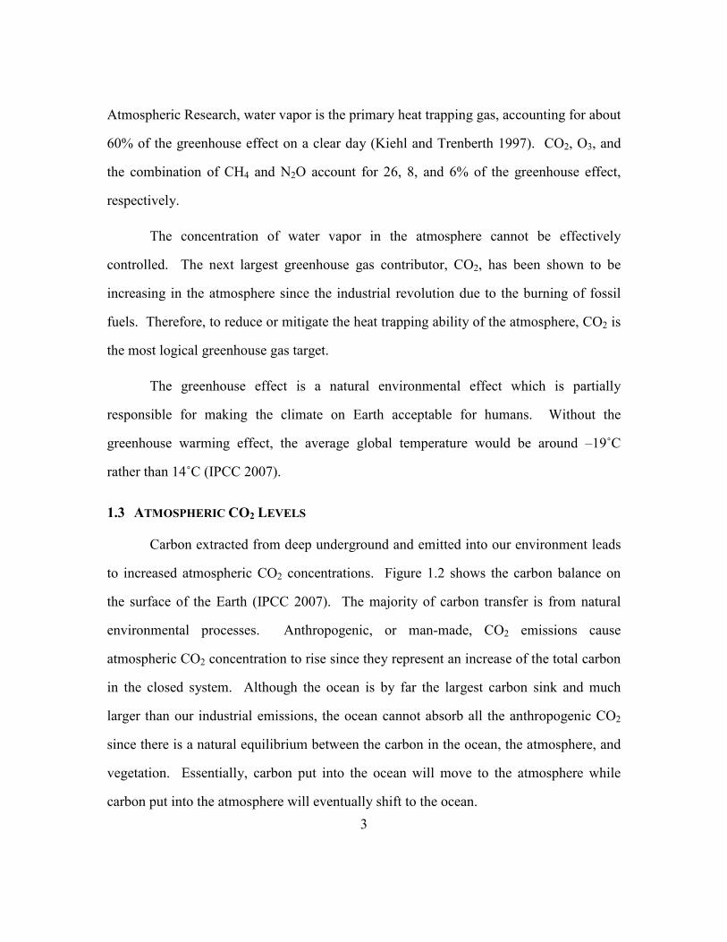
Atmospheric Research, water vapor is the primary heat trapping gas, accounting for about

60% of the greenhouse effect on a clear day (Kiehl and Trenberth 1997). CO2, O3, and

the combination of CH4 and N2O account for 26, 8, and 6% of the greenhouse effect,

respectively.

The concentration of water vapor in the atmosphere cannot be effectively

controlled. The next largest greenhouse gas contributor, CO2, has been shown to be

increasing in the atmosphere since the industrial revolution due to the burning of fossil

fuels. Therefore, to reduce or mitigate the heat trapping ability of the atmosphere, CO2 is

the most logical greenhouse gas target.

The greenhouse effect is a natural environmental effect which is partially

responsible for making the climate on Earth acceptable for humans. Without the

greenhouse warming effect, the average global temperature would be around –19˚C

rather than 14˚C (IPCC 2007).

1.3 ATMOSPHERIC CO2 LEVELS

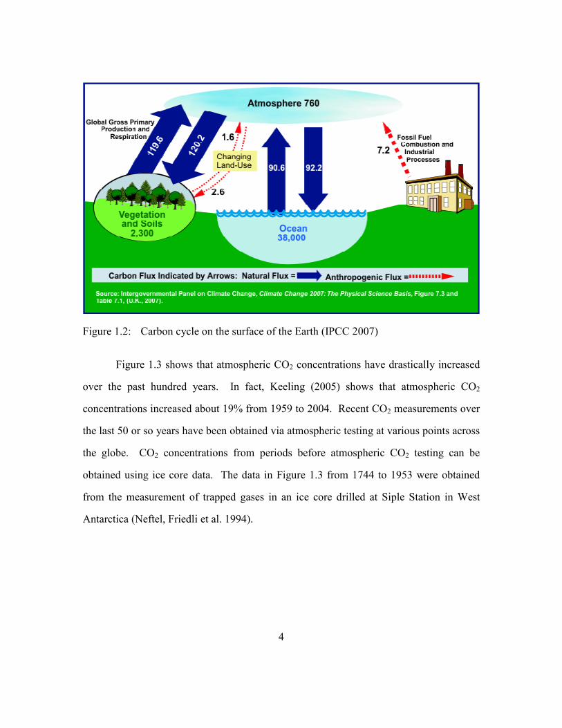
Carbon extracted from deep underground and emitted into our environment leads

to increased atmospheric CO2 concentrations. Figure 1.2 shows the carbon balance on

the surface of the Earth (IPCC 2007). The majority of carbon transfer is from natural

environmental processes. Anthropogenic, or man-made, CO2 emissions cause

atmospheric CO2 concentration to rise since they represent an increase of the total carbon

in the closed system. Although the ocean is by far the largest carbon sink and much

larger than our industrial emissions, the ocean cannot absorb all the anthropogenic CO2

since there is a natural equilibrium between the carbon in the ocean, the atmosphere, and

vegetation. Essentially, carbon put into the ocean will move to the atmosphere while

carbon put into the atmosphere will eventually shift to the ocean.

4

Figure 1.2: Carbon cycle on the surface of the Earth (IPCC 2007)

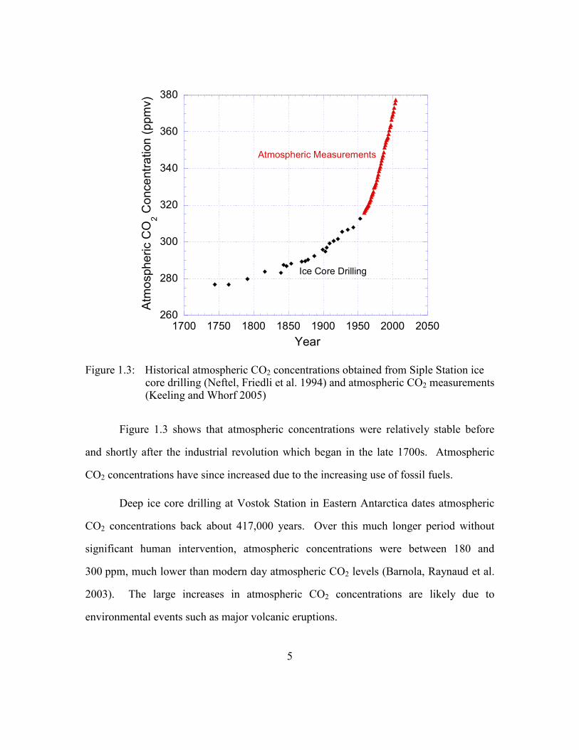
Figure 1.3 shows that atmospheric CO2 concentrations have drastically increased

over the past hundred years. In fact, Keeling (2005) shows that atmospheric CO2

concentrations increased about 19% from 1959 to 2004. Recent CO2 measurements over

the last 50 or so years have been obtained via atmospheric testing at various points across

the globe. CO2 concentrations from periods before atmospheric CO2 testing can be

obtained using ice core data. The data in Figure 1.3 from 1744 to 1953 were obtained

from the measurement of trapped gases in an ice core drilled at Siple Station in West

Antarctica (Neftel, Friedli et al. 1994).

5

260

280

300

320

340

360

380

1700 1750 1800 1850 1900 1950 2000 2050

Atm

ospheric CO

2 Concentration (ppmv)

Year

Atmospheric Measurements

Ice Core Drilling

Figure 1.3: Historical atmospheric CO2 concentrations obtained from Siple Station ice core drilling (Neftel, Friedli et al. 1994) and atmospheric CO2 measurements (Keeling and Whorf 2005)

Figure 1.3 shows that atmospheric concentrations were relatively stable before

and shortly after the industrial revolution which began in the late 1700s. Atmospheric

CO2 concentrations have since increased due to the increasing use of fossil fuels.

Deep ice core drilling at Vostok Station in Eastern Antarctica dates atmospheric

CO2 concentrations back about 417,000 years. Over this much longer period without

significant human intervention, atmospheric concentrations were between 180 and

300 ppm, much lower than modern day atmospheric CO2 levels (Barnola, Raynaud et al.

2003). The large increases in atmospheric CO2 concentrations are likely due to

environmental events such as major volcanic eruptions.

6

160

180

200

220

240

260

280

300

320

01 105

2 105

3 105

4 105

Atmospheric CO

2 Concentration (ppmv)

Year (BC)

Figure 1.4: Historical CO2 concentration measured from the Vostok ice core (Barnola, Raynaud et al. 2003)

1.4 CO2 EMISSIONS

If atmospheric CO2 concentrations are to be prevented from increasing

indefinitely at a fast rate, anthropogenic CO2 emissions to the atmosphere must be

limited. Before addressing the limiting of CO2 emissions, it is important to understand

where the man-made CO2 emissions originate in order to target a specific source.

The Energy Information Administration maintains the official energy statistics for

the U.S. government. Figure 1.5 shows the world CO2 emissions for petroleum, coal, and

natural gas (EIA 2008a).

7

4

6

8

10

12

1980 1985 1990 1995 2000 2005

World CO

2 Emissions

(Billion (109) Metric Tons of CO

2/yr)

Year

Coal

Petroleum

Natural Gas

Figure 1.5: World CO2 emissions from fossil fuels (EIA 2008a)

Coal and petroleum account for the majority of CO2 emissions. Petroleum is

generally used as a transportation fuel for vehicles, which results in a very large number

of small emission sources. In the U.S. about 90% of coal is used for electricity

generation (EIA 2008b). These large coal-fired power plants represent a significant

portion of the total CO2 emissions and are sufficiently large emission sources to address

capturing CO2.

1.5 AQUEOUS AMINE ABSORPTION/STRIPPING

Aqueous amine absorption/stripping is a mature technology which is capable of

capturing CO2 emissions from a coal-fired power plant. It has the advantage of being a

tail-end process which can be added on to an existing power plant. A flowsheet of a

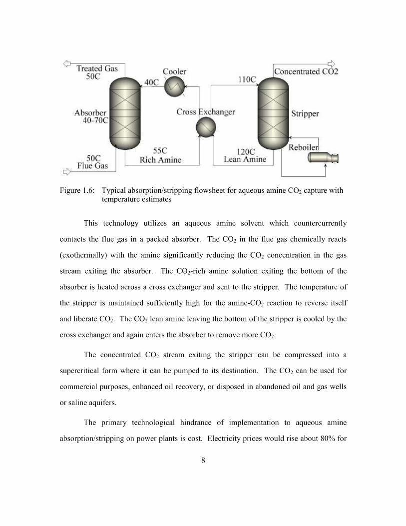
typical aqueous amine absorption/stripping system is shown in Figure 1.6.

8

Figure 1.6: Typical absorption/stripping flowsheet for aqueous amine CO2 capture with temperature estimates

This technology utilizes an aqueous amine solvent which countercurrently

contacts the flue gas in a packed absorber. The CO2 in the flue gas chemically reacts

(exothermally) with the amine significantly reducing the CO2 concentration in the gas

stream exiting the absorber. The CO2-rich amine solution exiting the bottom of the

absorber is heated across a cross exchanger and sent to the stripper. The temperature of

the stripper is maintained sufficiently high for the amine-CO2 reaction to reverse itself

and liberate CO2. The CO2 lean amine leaving the bottom of the stripper is cooled by the

cross exchanger and again enters the absorber to remove more CO2.

The concentrated CO2 stream exiting the stripper can be compressed into a

supercritical form where it can be pumped to its destination. The CO2 can be used for

commercial purposes, enhanced oil recovery, or disposed in abandoned oil and gas wells

or saline aquifers.

The primary technological hindrance of implementation to aqueous amine

absorption/stripping on power plants is cost. Electricity prices would rise about 80% for

9

coal-fired power plants that employ CO2 capture (Rubin, Rao et al. 2004). About 80% of

that price increase is associated with the capture and compression of CO2 while the

remaining 20% is attributed to sequestration (Rao and Rubin 2002). In an effort to

reduce the cost of carbon capture, alternative amine solvents are being researched.

Currently, 30 wt% monoethanolamine (MEA) is considered the baseline solvent for

aqueous amine absorption/stripping. Alternative solvents may provide faster rates, higher

CO2 capacities, better degradation or corrosion properties, or better thermodynamic

properties, which affect how CO2 capture systems are operated. New solvents provide

the opportunity to obtain significant energy and capital cost savings.

1.6 SCOPE OF WORK

The focus of this work is to compare CO2 reaction rates of other amine systems to

the current standard, MEA. Numerous experimental studies quantifying reaction rates

have been performed on MEA and other amines (Versteeg, Van Dijck et al. 1996).

However, very little of this work has been performed with concentrated amine solutions

which will be required for CO2 capture from flue gas. Industrial systems will also utilize

CO2 loaded amine solutions since liberating all the CO2 from the solution is unreasonable

due to energy costs. Very little literature data has been compiled for CO2 loaded amines.

Highly concentrated, highly loaded amine systems are non-ideal solutions which provide

a completely different ionic environment than dilute, unloaded amine solutions. These

dilute, unloaded experimental results do not translate to industrial solutions.

Overall, there is a lack of kinetic data for the CO2 absorption/desorption rates into

highly concentrated, highly CO2 loaded amine solutions. This work provides the first

comprehensive rate study on CO2 loaded, concentrated piperazine solutions (2–12 m) at

both absorber and stripper temperatures. This work also provides a second major rate

10

study on CO2 loaded, concentrated monoethanolamine solutions (7–13 m).

7 m MEA/2 m PZ solutions have also been studied in the wetted wall column.

Due to some uncertainty in the viscosity-diffusion coefficient relationship for

various amine systems, diaphragm cell diffusion experiments were conducted with MEA

and PZ solutions. These systems have also been modeled to explain the observed mass

transfer behavior.

11

Chapter 2: Literature Review

Absorption involves the mass transfer of a substance from the gas phase into the

liquid phase. The absorbed substance may be either physically or chemically bound in

the solvent. Physical solvents are often used to absorb CO2 in high pressure

environments like natural gas treating. The CO2 solubility in physical solvents decreases

with decreasing pressure and is inadequate for flue gas applications. CO2 capture from

flue gas requires a chemical solvent. Amine solvents react chemically with dissolved

CO2 and store it in a carbamate or bicarbonate form. Amines are organic compounds that

contain a basic nitrogen atom.

2.1 GENERAL AMINE CHEMISTRY

Amines are generally subdivided by structure. Primary amines have nitrogen

atoms connected to one carbon atom. Secondary amines have nitrogen atoms connected

to two carbon atoms. Both primary and secondary amines provide open structures that

allow CO2 to reach the nitrogen and form carbamates. Tertiary amines have three carbon

atoms connected to the nitrogen. This crowded environment around the nitrogen

prevents carbamate stability. Tertiary amines produce bicarbonate instead of carbamates.

Hindered amines are primary or secondary amines which have bulky groups around the

nitrogen. Hindered amines are defined as either a) primary amines in which the nitrogen

is attached to a tertiary carbon or b) secondary amines in which the nitrogen is attached to

a secondary or tertiary carbon (Satori and Savage 1983). The degree of hindrance will

12

determine if the hindered amine is capable of producing some carbamate or only

bicarbonate. Equations 2.1–2.4 show chemical structures for a primary

(monoethanolamine), secondary (diethanolamine), tertiary (triethanolamine), and

hindered amine (AMP).

HONH2

(2.1)

HO

HN

OH (2.2)

HON

OH

OH

(2.3)

C

CH3

CH3

NH2HO

(2.4)

2.1.1 Monoethanolamine and Piperazine

The focus of this work is on monoethanolamine (MEA) and piperazine (PZ)

solutions. Piperazine is a secondary amine with two amine groups, providing a large CO2

capacity. Its cyclic structure exposes the nitrogen groups and results in very fast reaction

with CO2. The ring structure also provides increased resistance against thermal

degradation allowing for stripping at higher temperatures (Davis 2009). The structure of

piperazine is shown in Equation 2.5.

NHHN

(2.5)

Aqueous monoethanolamine and piperazine solutions will form carbamates and

bicarbonate when reacted with CO2. The MEA carbamate reaction is shown generically

in Equation 2.6. The possible piperazine carbamate reactions are listed in Equations 2.7–

13

2.9. The bicarbonate reaction shown in Equation 2.10 can become significant in both

MEA and piperazine systems at high CO2 loading.

+− +↔++ BHMEACOOBCOMEA 2 (2.6)

+− +↔++ BHPZCOOBCOPZ 2 (2.7)

( ) +−− +↔++ BHCOOPZBCOPZCOO 22 (2.8)

+−++ +↔++ BHPZCOOHBCOPZH 2 (2.9)

+− +↔++ BHHCOBCOOH 322 (2.10)

Component B can be any base in the system. Bases in MEA and PZ systems

include: MEA, PZ, PZH+, PZCOO

–, H2O, and OH

–. PZH

+ and OH

– are not significant

bases in the system since PZH+ has a very low pKa and OH

– is not present in significant

concentrations. The low pKa of PZH+ also suggests via Bronsted theory that the forward

rate constant of Equation 2.9 will be several orders of magnitude slower than the forward

rate constants of Equations 2.7 and 2.8. Derks et al. (2006) has shown that the reaction in

Equation 2.9 is a very small contributor to the CO2 absorption.

2.1.2 CO2 Loading

The CO2 loading is a measurement of the CO2 concentration in the solution. It is

defined as the ratio of CO2 molecules to alkalinity (active nitrogen) groups. MEA has

one alkalinity group per molecule while piperazine has two. For an MEA, PZ, or

MEA/PZ system, the definition of CO2 loading is expressed mathematically in Equation

2.11.

PZMEA

CO

nn

nLoadingCO

2

2

2 +=

(2.11)

14

2.2 MASS TRANSFER WITH FAST REACTION

2.2.1 Zwitterion Reaction Mechanism

Absorption of CO2 by amines such as MEA and piperazine is often explained by

the zwitterion mechanism, originally proposed by Caplow (1968) and reintroduced by

Danckwerts (1979). The zwitterion is an ionic, but neutrally charged intermediate that is

formed from the reaction of CO2 with an amine. The zwitterion mechanism for

carbamate formation is a two step process: the CO2 reacts with the amine to form a

zwitterion, followed by the extraction of a proton by a base. In the following example

water acts as the base. For simplicity the zwitterion mechanism is shown with the usual

convention of irreversible proton extraction.

C

O

O

+NH

R

R'kf

krN+

R'

R H

C O

O-

(2.12)

N+

R'

R H

C O

O-

N C

O

O-

R

R'

O+

H H

H

OH

H

+ +

kb

(2.13)

The two step zwitterion mechanism leads to the CO2 absorption rate shown in

Equation 2.14.

∑+

−=

][

1

]][[ 22

Bkk

k

k

COAmr

bf

r

f

CO (2.14)

Bases can include the amine as well as H2O and OH–. In some systems H2O and

OH– can contribute pronounced effects to the rate of reaction (Blauwhoff, Versteeg et al.

1983). For MEA, the zwitterion is protonated fast in comparison to the reversion rate to

MEA and CO2 (Danckwerts 1979). Since [ ]∑ Bkb is much greater than rk for MEA,

Equation 2.14 simplifies to Equation 2.15.

15

[ ][ ]22 COMEAkr fCO −= (2.15)

For many secondary amines, a second order reaction with respect to the amine is

observed. This implies that for secondary amines rk is much greater than [ ]∑ Bkb

yielding Equation 2.16.

[ ][ ]∑−= ][22 BkCOMEAk

kr b

r

f

CO (2.16)

The zwitterion mechanism can also be solved with a reversible base protonation

step. This causes the reaction in Equation 2.13 to be replaced by Equation 2.17.

N+

R'

R H

C O

O-

N C

O

O-

R

R'

O+

H H

H

OH

H

+ +k-b

kb

(2.17)

This leads to the following form of the rate equation, which now includes a

driving force for the reversion of carbamate to amine and CO2.

−+

−=∑

∑

∑

+−

]][[

]][[

][

][

1

][ ,

22BAmk

BHAmCOOK

k

CO

Bkk

k

k

Amr

b

beq

b

bf

r

f

CO (2.18)

The Keq,b term in Equation 2.18 is the overall equilibrium constant and is specific

to the base pathway. For unloaded solutions, the reverse portion of Equation 2.18 can be

ignored to produce the irreversible result of Equation 2.14. If the concentrations of the

reactants and products are at equilibrium, the equilibrium constant will reduce the

reversible term to [CO2] which will yield a zero for the rate of CO2 formation.

16

2.2.2 Termolecular Reaction Mechanism

Contrary to the zwitterion mechanism, Crooks and Donnellan (1989) presented

the termolecular mechanism, which assumes the reaction proceeds via a loosely bound

complex. The complex and the reaction mechanism are shown in Equation 2.19.

N:

R

H

R

B:

C

O

O

(2.19)

This mechanism coincides with the limiting case for the zwitterion mechanism

where rk is much greater than [ ]∑ Bkk bf . The rate of CO2 absorption is identical to the

zwitterion result shown in Equation 2.16.

It is theorized that most of the loosely bound complexes break up to produce

reagent molecules again while a few react with a second molecule of amine or water to

yield ionic products (Crooks and Donnellan 1989). The bond formation and charge

separation occur in the second step.

Since both the zwitterion and termolecular reaction mechanisms allow for varying

orders of the amine concentration, both can be fitted to experimental data. An equally

effective representation of reaction rates should be possible using either mechanism.

2.2.3 Film Theory

Mass transfer of CO2 from the gas phase into the liquid phase is a film resistance

process. Figure 2.1 shows a typical film analysis for CO2 absorption with fast reaction.

17

Figure 2.1: Mass transfer of CO2 into the bulk liquid with fast chemical reaction

Gaseous CO2 molecules diffuse through the gas film to the gas-liquid interface.

At the gas-liquid interface the gaseous CO2 dissolves according to the Henry’s solubility.

The dissolved CO2 is significantly depleted near the interface due to reaction with the

amine, while the CO2 diffuses to the bulk liquid.

The slope of the CO2 concentration profile defines the mass transfer coefficients.

Equations 2.20–2.23 describe the flux equations which can be written using the overall

mass transfer coefficient (KG), gas film mass transfer coefficient (kg), or a liquid film

mass transfer coefficient (kl or kg’). kl is the liquid film mass transfer coefficient. kg’ is

the liquid film mass transfer coefficient defined in gas film units. kg’ is convenient to use

since partial pressures, not liquid phase concentrations, are experimentally measured. No

Henry’s constant assumptions are required. klo is the physical liquid film mass transfer

coefficient, which does not incorporate reaction.

18

)( *

,2,22 bCObCOGCO PPKN −= (2.20)

)( ,2,22 iCObCOgCO PPkN −= (2.21)

)][]([ 222 bilCO COCOkN −= (2.22)

)( *

,2,2

'

2 bCOiCOgCO PPkN −= (2.23)

The flux in Equations 2.20–2.23 is constant, and Equations 2.20, 2.21 and 2.23

can be combined. Combining these three equations yields a series resistance relationship

between the mass transfer coefficients.

'

111

ggG kkK+= (2.24)

Since kg’ encompasses the reaction and the liquid phase diffusion films, it has

both a reaction and a diffusion component. These two components can be separated as

shown in Equation 2.25. The first term, kg’’, is the pseudo first order term which

represents the reaction kinetics of the amine. The second term represents diffusion

resistance and depends on the liquid film physical mass transfer coefficient and the slope

of the equilibrium line.

[ ]

∆

∆++=

T

o

ggG CO

P

kkkK

CO

prodl 2

*

''

2

,

1111 (2.25)

The problem with separating kg’ into these two terms is that these terms are

difficult to quantify, particularly the slope of the equilibrium curve, which is extremely

steep. Separating kg’ into these two terms generally introduces significant error. Results

in the current work are reported as kg’ values.

The third term in Equation 2.25, which includes the slope of the equilibrium line,

results from changing a concentration driving force to a partial pressure driving force to

19

enable a series resistance relationship with KG, kg, and kg’’. Equation 2.26 shows the

transition using the film schematic shown in Fig 2.1 where RDint denotes the reaction-

diffusion interface.

[ ] [ ]( ) [ ] [ ] ( )bCORDCO

bCORDCO

bRDo

lbRD

o

lCO PPPP

COCOkCOCOkN ,2int,2

,2int,2

2int2

2int22 −

−

−=−= (2.26)

As Figure 2.1 shows, there is a gas film resistance, a reaction resistance, and a

liquid film diffusion resistance. A system in which the liquid phase diffusion is

unimportant leads to the pseudo first order condition. A system in which the reaction

resistance is negligible leads to the instantaneous reaction condition. The gas film

resistance can be negligible but this case does not require special consideration. It is also

possible for two resistances to be negligible.

2.2.4 Pseudo First Order Reaction

The pseudo first order approximation is a simplification to mass transfer with fast

reaction in which the liquid reactant and product concentrations are assumed constant

throughout the liquid boundary layer. It assumes that the liquid phase diffusion

resistance is negligible. This assumption may be justified at high free amine

concentrations, low CO2 fluxes, or at high liquid film physical mass transfer coefficient

conditions.

A material balance of a fixed volume requires that the change in flux of dissolved

CO2 must be the result of reaction. A CO2 material balance for absorption is shown in

Equation 2.27.

0]][[][

22

2

2

2 =−∂

∂COAmk

x

COD fCO (2.27)

20

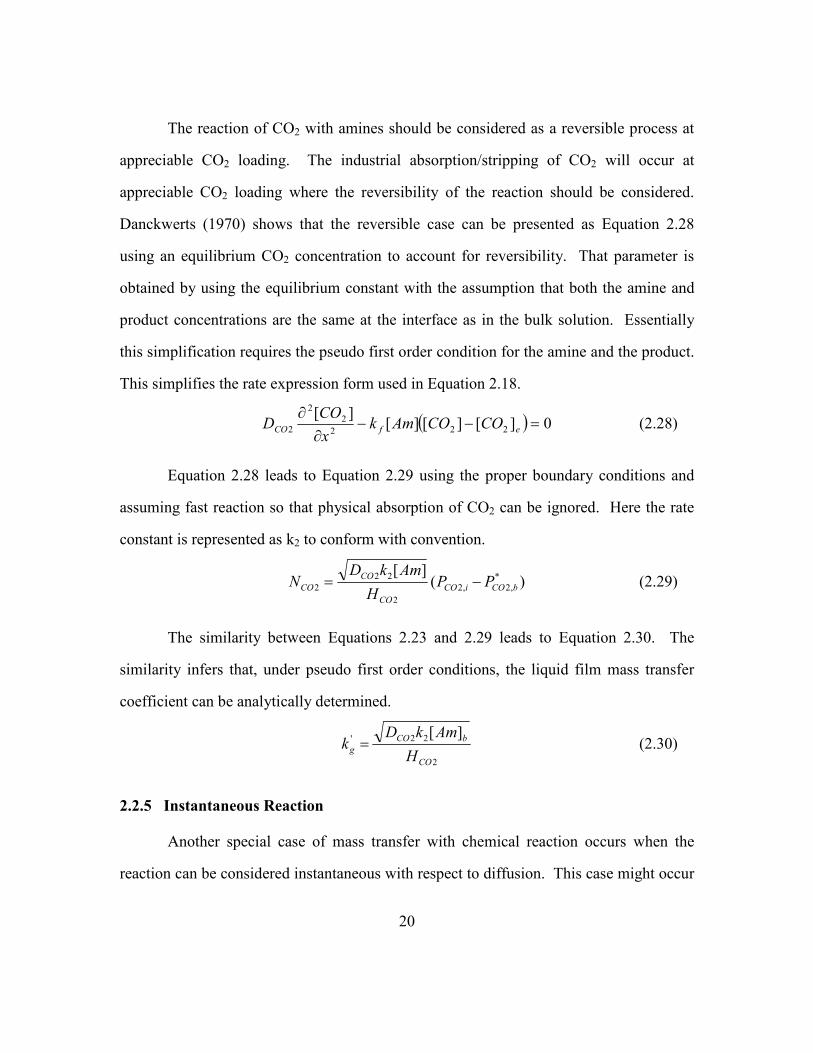
The reaction of CO2 with amines should be considered as a reversible process at

appreciable CO2 loading. The industrial absorption/stripping of CO2 will occur at

appreciable CO2 loading where the reversibility of the reaction should be considered.

Danckwerts (1970) shows that the reversible case can be presented as Equation 2.28

using an equilibrium CO2 concentration to account for reversibility. That parameter is

obtained by using the equilibrium constant with the assumption that both the amine and

product concentrations are the same at the interface as in the bulk solution. Essentially

this simplification requires the pseudo first order condition for the amine and the product.

This simplifies the rate expression form used in Equation 2.18.

( ) 0][][][][

222

2

2

2 =−−∂

∂efCO COCOAmk

x

COD (2.28)

Equation 2.28 leads to Equation 2.29 using the proper boundary conditions and

assuming fast reaction so that physical absorption of CO2 can be ignored. Here the rate

constant is represented as k2 to conform with convention.

)(][

*

,2,2

2

22

2 bCOiCO

CO

CO

CO PPH

AmkDN −= (2.29)

The similarity between Equations 2.23 and 2.29 leads to Equation 2.30. The

similarity infers that, under pseudo first order conditions, the liquid film mass transfer

coefficient can be analytically determined.

2

22'][

CO

bCO

gH

AmkDk = (2.30)

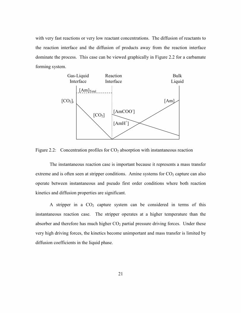
2.2.5 Instantaneous Reaction

Another special case of mass transfer with chemical reaction occurs when the

reaction can be considered instantaneous with respect to diffusion. This case might occur

21

with very fast reactions or very low reactant concentrations. The diffusion of reactants to

the reaction interface and the diffusion of products away from the reaction interface

dominate the process. This case can be viewed graphically in Figure 2.2 for a carbamate

forming system.

Gas-Liquid

Interface

Reaction

Interface

Bulk

Liquid

[Am]

[CO2] [AmCOO

-]

[Am]Total

[CO2]i

[AmH+]

Figure 2.2: Concentration profiles for CO2 absorption with instantaneous reaction

The instantaneous reaction case is important because it represents a mass transfer

extreme and is often seen at stripper conditions. Amine systems for CO2 capture can also

operate between instantaneous and pseudo first order conditions where both reaction

kinetics and diffusion properties are significant.

A stripper in a CO2 capture system can be considered in terms of this

instantaneous reaction case. The stripper operates at a higher temperature than the

absorber and therefore has much higher CO2 partial pressure driving forces. Under these

very high driving forces, the kinetics become unimportant and mass transfer is limited by

diffusion coefficients in the liquid phase.

22

2.2.6 Bronsted Theory

A significant amount of work on acid-base catalysis was performed by Bronsted

(1928). This work provided an important link between equilibrium strength and reaction

rates. Ka is the equilibrium constant of the dissociation of an acid which is written with

respect to water. A designates the acid and A– designates the base.

+− +→←+ OHAOHA aK

32 (2.31)

Ka is representative of the strength of an acid (or base) and is generally referred in

terms of the pKa defined in Equation 2.32.

aa KpK 10log−= (2.32)

Base catalysis has been widely recognized as a contributing factor in CO2 reaction

rates with amines. Both the zwitterion and termolecular reaction mechanisms can

account for acid-base catalysis. Data compiled by Rochelle et al. (2001) show the

correlation between rate constants and pKa for primary, unhindered amines. Similarly,

the pKa of an extracting base can affect CO2 reaction rates.

23

0.01

0.1

1

10

100

5 6 7 8 9 10 11

Primary Amines @ 25C

k2 (m

3/mol.s)

pKa

Figure 2.3: Bronsted correlation of CO2 reaction rates for unhindered, primary amines at 25˚C (Rochelle, Bishnoi et al. 2001)

2.2.7 Mass Transfer Contactors

Various gas-liquid contactors are used to measure absorption or desorption of

CO2 in amine systems. Each contactor has advantages and disadvantages. Three of the

more common contactors are briefly introduced here. Each type of contactor may also

have multiple versions with unique characteristics but the operating concept for the

contactor remains the same.

2.2.7.1 Stirred Cell

The stirred cell is a gas-liquid contactor which operates with a smooth, horizontal

gas-liquid interface. This smooth interface is vital in preserving the known contact area

for the reaction. The gas and liquid phases can be mixed independently using magnetic

stirrers. This allows for both gas and liquid phases to remain homogeneous during CO2

24

mass transfer. Gaseous CO2 can be introduced into the cell at the start of the experiment,

pressurizing the cell. The pressure can be measured as a function of time to determine

the rate at which the gaseous CO2 is reacting with the solvent. Derks et al. (2006) is

among recent researchers who measure reaction rates using a stirred cell. Figure 2.4

shows a schematic of the stirred cell Derks utilized.

Figure 2.4: Schematic of a stirred cell contactor (Derks, Kleingeld et al. 2006)

The main advantage of the stirred cell is its simplicity. Also, the rate of

absorption is measured using a liquid having a single, known composition, assuming klo

is sufficiently large.

The disadvantages of the stirred cell include the limitations in klo. A homogenous

liquid is required but the solution must not be stirred to the point that the gas-liquid

interface is agitated. A fast reaction with large CO2 fluxes can create possible

concentration differences at the gas-liquid interface. The value of klo can also be

sensitive to the immersion depth of the liquid phase stirrer (Danckwerts 1970). The

volume of liquid in a stirred cell apparatus is much larger than a packed column so any

25

systems which include significant bulk liquid reactions cannot be modeled using this

apparatus. It is also difficult to get large values of kg so conditions where CO2 is diluted

can be difficult to interpret.

2.2.7.2 Laminar Jet

The laminar jet absorber shoots a jet of liquid through a tiny circular hole. The

solvent contacts a CO2-rich gas phase over a known height before re-entering a slightly

larger hole. The jet can be considered a cylindrical rod in uniform motion. Typically the

jet is about 1 mm in diameter and a few cm in length. The time of exposure can be

determined by the jet height and velocity. The jet is housed in a closed, CO2 rich

environment in which the pressure can be monitored to determine the rate of CO2

absorption. Aboudheir et al. (2003) is among recent researchers who used a laminar jet

absorber. Figure 2.5 shows a schematic of the laminar jet absorber Aboudheir used.

Figure 2.5: Schematic of a laminar jet contactor (Aboudheir, Tontiwachwuthikul et al. 2003)

26

The laminar jet absorber has the advantage of having very short contact times and

therefore very large klo values. At most conditions the free amine at the surface cannot be

appreciably depleted from the top to the bottom of the contactor due to the short contact

time. Often the contact length of the jet can be adjusted. The laminar jet absorber is well

suited to measure absorption rates in fast systems.

The laminar jet requires the selection of a suitable nozzle or orifice to ensure a

uniform jet velocity as well as the convergence of the jet at the bottom of the contactor.

The laminar jet absorber requires several tens of liters of solution for a comprehensive

series of measurements (Danckwerts 1970).

2.2.7.3 Wetted Wall Column

In a wetted wall column the liquid flows in a film, under the influence of gravity,

down a surface, usually a tube or rod. The contacting gas flows countercurrent to the

liquid and mass transfer occurs over the gas-liquid contact area. The rigid tube or rod has

a known surface area which is entirely coated by the thin film of solvent. The length of

the rod can be adjustable to vary the contact time and thus vary the liquid film physical

mass transfer coefficient. A wetted wall column contactor has been used in this work.

The same wetted wall column was used by previous researchers (Bishnoi and Rochelle

2000; Cullinane and Rochelle 2006).

27

Figure 2.6: Schematic of the wetted wall column contactor used in this work

One major advantage of the wetted wall column is its versatility. It can operate

over a wide range of conditions and can absorb or desorb CO2 equally well. The klo

values for the wetted wall column can also be easily compared to packed columns by

comparing the flow path lengths. Wetted wall columns have high klo values allowing

them to measure fast reacting amines.

Among the concerns of the wetted wall column are the entrance effects. It is

important that the solvent is evenly dispersed so that a uniform film coats the entire

surface of the rod. Any dry spots on the surface of the rod will not contribute to the flux

and will lead to erroneous calculations. It is important to prevent the solution from

28

rippling as it flows down the side of the contactor. The ripples enhance the liquid film

physical mass transfer coefficient, klo, and may affect the rate of absorption.

2.3 RATE STUDIES

2.3.1 Quantifying Reaction Rates

Rate studies for CO2 absorption rates with amines usually publish rate constants

as the culmination of the work. However, rate constants can be misleading. Higher rate

constants do not necessarily correspond with faster reaction. Systems that adhere to the

pseudo first order assumption have fluxes that can be represented by Equation 2.33.

)(][

*

,2,2

2

22

2 bCOiCO

CO

CO

CO PPH

AmkDN −= (2.33)

It is true that increasing the rate constant in Equation 2.33 will lead to a higher

flux, but that does not mean that another system with a slower rate constant will have

slower fluxes. The important parameter is not the rate constant but the mass transfer

coefficient, the group of terms multiplied by the driving force. Therefore, it is important

to consider all the aspects of the mass transfer coefficient, not just the rate constant.

Imagine two amine systems with similar rate constants, diffusion coefficients, and

free amine concentrations. If one of those systems has a higher CO2 solubility (1/HCO2)

in the liquid phase, it will achieve higher CO2 absorption rates because there are many

more reactants present. This concern is ignored analytically by the convention that

Henry’s constants are usually calculated as the CO2 solubility in water. That may be an

acceptable assumption for much of the kinetic literature data, since dilute, unloaded

solutions are typically used. However in industrial application, particularly CO2 capture

from flue gas, concentrated, CO2 loaded solutions will be used. These highly

concentrated, ionic solutions will not have CO2 activity coefficients of 1.0. Browning

29

and Weiland (1994) have shown that the effective Henry’s constant in 30 wt% MEA

varies from 4800 Pa.m

3/mol at 0 CO2 loading to 7400 Pa

.m

3/mol at 0.35 loading. This

decreased CO2 solubility at higher CO2 loading is significant and should be included in

reaction rate considerations. The Henry’s constant affects the flux to the first power

while the diffusion coefficient, rate constant, and free amine concentration only have a

0.5 power dependence.

There is also a more subtle rate consideration involving partial pressure and

speciation. The focus of this work is on CO2 capture from flue gas, particularly flue gas

from coal-fired power plants. In that case, the inlet CO2 concentration is likely in the

12% or 12,000 Pa partial pressure range at the bottom of the absorber. It is desirable to

obtain a CO2 rich solution which may have a CO2 partial pressure in the 5,000 Pa range.

At a 5 kPa CO2 partial pressure, different amine solutions will have different CO2

loadings. If two carbamate producing amines have CO2 loadings of 0.25 and 0.5 at a

5 kPa CO2 partial pressure, these solutions will have drastically different free amine

concentrations. The amine system at 0.25 loading may have ten times more free amine

than the other. Since the free amine concentration is a component of the mass transfer

coefficient, it will affect CO2 mass transfer. The kinetics at rich solution conditions are

the most vital for CO2 capture. The rich solution reacts slowest and therefore the

majority of the absorber column must contain relatively rich amine solution. This subtle

speciation consideration may warrant consideration for some amine systems.

Both the Henry’s constant and speciation concerns can be simply addressed by

reporting mass transfer coefficients at conditions typical of industrial processes, in this

case CO2 capture from coal-fired power plant flue gas. In the current work, rate

constants are not reported. A liquid phase mass transfer coefficient, kg’, is reported over

30

a range of applicable CO2 capture partial pressures. kg’ is defined in Equation 2.34. In

the pseudo first order case, kg’ is the grouping of terms including the diffusion

coefficient, rate constant, free amine concentration, and Henry’s constant.

)( *

,2,2

2'

bCOiCO

CO

gPP

Nk

−= (2.34)

In summary of this section, when comparing two amine systems a higher rate

constant does not necessarily correspond to faster CO2 mass transfer. A higher kg’

always corresponds to faster CO2 mass transfer when tested at proper industrial

conditions.

Regardless of the weaknesses of rate constants, almost all of the literature data is

presented in terms of rate constants. Since kg’ data is generally not available, rate

constant data is the best measure available to compare CO2 reaction rates in various

amine systems.

2.3.2 MEA Systems

A significant amount of data is available on rate studies concerning the reaction of

CO2 and MEA. Table 2.1 characterizes the current literature data.

31

Table 2.1: Literature data on the reaction between CO2 and aqueous MEA

Although Table 2.1 includes a large amount of literature data for MEA kinetics,

little of it is directly applicable to industrial CO2 capture systems. Industrial systems

would likely operate at absorber temperatures ranging from 40 to 70˚C while the majority

of the literature data was collected near ambient conditions. Also, higher temperature

data by Leder (1971) and Littel et al. (1992) are likely erroneous due to experimental or

calculation inaccuracies (Versteeg, Van Dijck et al. 1996). The only CO2 loaded, large

Temp [MEA] Reference

(C) (mol/l)

(Jensen, Jorgensen et al. 1954) 18 0.1–0.2

(Astarita 1961) 21.5 0.25–2.0

(Emmert and Pigford 1962) 25 0.1–2.0

(Clarke 1964) 25 1.6–4.8

(Sharma 1965) 25–30 1.0

(Danckwerts and Sharma 1966) 18–35 1.0

(Leder 1971) 80 –

(Sada, Kumazawa et al. 1976a) 25 0.2–1.9

(Hikita, Asai et al. 1977) 5.4–35.2 0.02–0.18

(Alvarez-Fuster, Midoux et al. 1980) 20 0.2–2.0

(Donaldson and Nguyen 1980) 25 0.03–0.08

(Laddha and Danckwerts 1981a) 25 0.49–1.71

(Penny and Ritter 1983) 5–30 0–0.06

(Sada, Kumazawa et al. 1985) 30 0.5–2.0

(Barth, Tondre et al. 1986) 20–25 0.02–0.05

(Crooks and Donnellan 1989) 25 0.02–0.06

(Alper 1990) 5–25 0–0.45

(Littel, Versteeg et al. 1992) 45–60 0–3.2

(Dang and Rochelle 2003) 40–60 2.5–5.0

(Aboudheir, Tontiwachwuthikul et al. 2003) 20–60 3.0–9.1

(Jamal, Meisen et al. 2006) 20–110 0.7–5.0

(Hartono 2009) 25–50 0.5–5.0

32

data source above 40˚C is Aboudheir et al. (2003). However, laminar jet absorber results

from Aboudheir et al. are not easily comparable nor do they seem to coincide with the

literature data.

Industrial CO2 capture systems will operate at high amine concentrations with

CO2 loaded solutions. All of the data with the exception of those by Dang and Rochelle

(2003), Aboudheir et al. (2003), and Jamal et al. (2006) were collected using unloaded

solutions. Very little of the data besides these three sources was collected at significant

MEA concentrations. Industrial operation will likely require at least 4 M MEA to reduce

operational costs.

Although data by Jamal et al. include interesting conditions (unloaded absorption

experiments up to 50˚C and high temperature desorption experiments of loaded MEA

solutions), it is not particularly useful. Jamal does not report rate constants for MEA nor

provide raw data on the experimental conditions of the experiments.

Dang et al. provide useful kinetic results but only provide a total of seven data

points. Three CO2 loadings in 2.5 M MEA and four CO2 loadings in 5 M MEA were

examined.

The data collected by Aboudheir are the only valuable, major data source

applicable to CO2 capture systems. As previously mentioned, the extracted kinetics do

not seem to agree with other literature data. The difference may be due to the highly

concentrated, highly loaded, or highly non-ideal nature of these solutions. The

differences for ideal versus non-ideal systems highlight the need to perform rate studies

on amine systems similar to those expected for industrial systems. In addition to

explaining why the Aboudheir data do not agree with the literature data, the current work

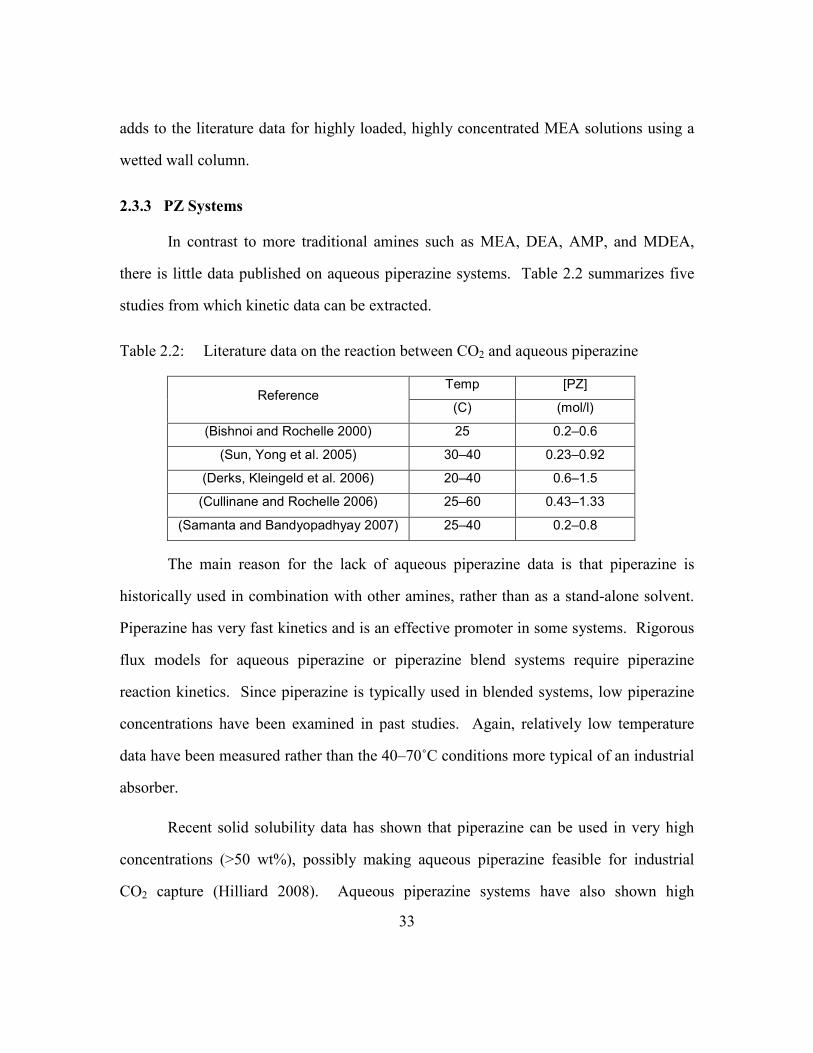
33

adds to the literature data for highly loaded, highly concentrated MEA solutions using a

wetted wall column.

2.3.3 PZ Systems

In contrast to more traditional amines such as MEA, DEA, AMP, and MDEA,

there is little data published on aqueous piperazine systems. Table 2.2 summarizes five

studies from which kinetic data can be extracted.

Table 2.2: Literature data on the reaction between CO2 and aqueous piperazine

The main reason for the lack of aqueous piperazine data is that piperazine is

historically used in combination with other amines, rather than as a stand-alone solvent.

Piperazine has very fast kinetics and is an effective promoter in some systems. Rigorous

flux models for aqueous piperazine or piperazine blend systems require piperazine

reaction kinetics. Since piperazine is typically used in blended systems, low piperazine

concentrations have been examined in past studies. Again, relatively low temperature

data have been measured rather than the 40–70˚C conditions more typical of an industrial

absorber.

Recent solid solubility data has shown that piperazine can be used in very high

concentrations (>50 wt%), possibly making aqueous piperazine feasible for industrial

CO2 capture (Hilliard 2008). Aqueous piperazine systems have also shown high

Temp [PZ] Reference

(C) (mol/l)

(Bishnoi and Rochelle 2000) 25 0.2–0.6

(Sun, Yong et al. 2005) 30–40 0.23–0.92

(Derks, Kleingeld et al. 2006) 20–40 0.6–1.5

(Cullinane and Rochelle 2006) 25–60 0.43–1.33

(Samanta and Bandyopadhyay 2007) 25–40 0.2–0.8

34

resistance to thermal degradation which can occur in the stripper and reboiler (Davis

2009).

Only the Bishnoi study in Table 2.2 was conducted with CO2 loaded amines. The

current work explores piperazine rates in loaded systems at higher temperatures and

much higher amine concentrations.

2.2.4 MEA/PZ Systems

Piperazine has historically been used as a promoter due to its fast reaction rates

and perceived low solubility. Piperazine activated aqueous MDEA, AMP, MEA, and

potassium carbonate have all been studied (Bishnoi and Rochelle 2000; Dang and

Rochelle 2003; Sun, Yong et al. 2005; Cullinane and Rochelle 2006).

Monoethanolamine is the fastest of these four solvents and is being evaluated in the

present work. Previous work on MEA/PZ solvents is scarce and is shown in Table 2.3.

Table 2.3: Literature data on the reaction between CO2 and MEA/PZ blends

Temp [MEA] [PZ] CO2 Loading Reference

(C) (mol/l) (mol/l) (mol/molalk)

40 0.4 0.6 0.06–0.14

40 1.9 0.6 0.01–0.44 (Dang and

Rochelle 2003) 40–60 3.8 1.2 0.41–0.43

(Okoye 2005) 40–60 4.4 1.2 0.28–0.57

Both literature sources for rate data on MEA/PZ systems study loaded systems.

Although Dang and Rochelle (2003) provide data for three different MEA/PZ solvent

blends, there is little data at each blend composition. Dang provides a total of seven data

points. Rate data by Okoye (2005) is similarly scarce. Okoye provides a total of six data

points from his MEA/PZ rate experiments. To complicate matters, data from Okoye does

not agree with Dang and seems unreasonable.

35

The current work seeks to expand the rate data for MEA/PZ blended systems by

evaluating 7 m MEA/2 m PZ.

2.4 DIFFUSION COEFFICIENT AND VISCOSITY CONSIDERATIONS

The current work uses a wetted wall column for rate measurements. CO2 mass

transfer in the wetted wall column, utilizing very fast, highly concentrated, highly loaded

amines is likely to be dependent on diffusion properties under some conditions. The

wetted wall column has a liquid flow path of 9.1 cm. Two-inch industrial packing likely

has an average liquid flow path 2–3 cm before remixing. The reduced liquid flow path in

packed columns results in a higher liquid film physical mass transfer coefficient, klo. The

higher mass transfer coefficient may result in negligible diffusion resistance in packed

columns but not in wetted wall column experiments. Therefore, it is very important to

understand the diffusion properties to extrapolate reaction rates in industrial columns.

Some researchers have produced viscosity-diffusion coefficient correlations to

account for physical property differences (Versteeg and Van Swaaij 1988; Snijder, te

Riele et al. 1993). The empirically regressed correlations do not provide first order

dependencies as the Wilke-Chang equation may suggest (Equation 2.35). Work by

Versteeg and Van Swaaij (1988) has shown that the diffusion of N2O and CO2 in aqueous

amines generally follows the viscosity dependence in Equation 2.36. Snijder et al. (1993)

have shown that alkanolamine diffusion in aqueous alkanolamine solutions follows the

viscosity dependence in Equation 2.37.

6.0

A

BB

ABV

TMD

⋅∝

µ

ψ (2.35)

( ) ( )WaterONeSolutionAON DCONSTANTD 8.0

2min

8.0

2 ηη == (2.36)

( ) ( )WatereAeSolutionAeA DCONSTANTD 6.0

minmin

6.0

min ηη == (2.37)

36

To make matters more complicated, the N2O and CO2 diffusivity relationship in

Equation 2.36 was confirmed with MDEA solutions but resulted in less satisfactory

results for AMP (Tomcej and Otto 1989; Xu, Otto et al. 1991). If the diffusion

relationships are dependent on amines, the relationship in Equation 2.36 may not directly

apply to MEA, piperazine, or MEA/PZ systems. The diffusion coefficient must be

determined for each system to evaluate rate data where both diffusion and reaction

kinetics affect mass transfer. The current work uses a diaphragm cell to measure

diffusion coefficients in monoethanolamine and piperazine systems.

37

Chapter 3: Experimental Methods

This chapter includes information on the experimental methods and apparatus

used in this work. A diaphragm cell was used to collect diffusion coefficient data in

MEA and PZ solutions. A wetted wall column was used to collect CO2 partial pressure

and CO2 rate data in MEA, PZ, and MEA/PZ solutions. Supporting equipment and

techniques used in the evaluation of data or experimental samples are also discussed.

3.1 DIAPHRAGM CELL

3.1.1 Diaphragm Cell Description

A diaphragm cell was built to measure diffusion coefficients in CO2 loaded amine

solutions. Diaphragm cells are recognized among the best diffusion coefficient

measuring devices because they are simple, rugged, and can be very accurate (Cussler

1997). Figure 3.1 shows a picture of the diaphragm cell used in these experiments.

The diaphragm cell consists of a glass tube with a glass frit at the midpoint. The

cell body is 13.8 cm tall and 4.1 cm in diameter. The frit is 4 mm thick with a 10–16 µm

pore size. The cell holds about 125 ml of solution during an experiment.

38

Figure 3.1: Diaphragm cell used in the experiments

Teflon end caps fitted with o-rings are used to maintain a closed system. Each

end cap also includes a 1/8” Swagelok male connector fitting which is threaded into the

end caps. The fitting allows air bubbles to be removed by injecting more solution with a

syringe. The male connector fitting can be capped when gas bubbles have been removed

from the cell.

Two stainless steel all thread rods are screwed into the inside of each of the

Teflon end caps. A stainless steel plate and bored out plastic screw cap are suspended

from the all thread rods. A glass rod is suspended through the bored plastic screw cap.

The glass rod attaches to a 4-armed glass stirrer which encases a magnet. The stirrer is

39

positioned a few millimeters from the frit. This ensures the solution composition near the

glass frit is the same as the bulk solution in that chamber.

The overall setup of the experiment can be seen in Figure 3.2. The diaphragm

cell is suspended vertically in a temperature bath. Two rotating magnets spin around the

cell causing the internal glass-encased magnets to mix the solution in each chamber. The

stirrer speed was set to 120 rpm. Over time, the solution from the top chamber will

diffuse into the bottom chamber and vice versa.

Figure 3.2: Schematic of the diaphragm cell experimental setup

3.1.2 Experimental Design

Diffusion experiments were conducted using 7–13 m MEA and 2–8 m PZ. For

each amine concentration a low CO2 loading and a high CO2 loading experiment were

conducted. In a typical low CO2 loading experiment for MEA, a solution with a 0.25

loading was placed in the top chamber and a 0.35 CO2 loading solution was placed in the

bottom chamber. In every experiment, the solution with the higher loading was placed in

the bottom chamber. Special care was taken to remove all air bubbles. Air bubbles from

40

the bottom chamber can rise to the glass frit and reduce the effective surface area for

diffusion.

Warmer temperatures reduce the length of the experiment since diffusion occurs

faster at higher temperatures where viscosities are lower. However, warmer solutions

present a thermal expansion concern which can loosen one of the end caps. If the

solution expands, pressure instead of diffusion may drive one solution into the other

chamber. To reduce the thermal expansion concern, all experiments were conducted at

30˚C. The required experimental time varied substantially depending on the viscosity of

the solution. Experiments ranged from 3–17 days. 12 m PZ experiments are not reported

because significant CO2 loading changes were not observed even after very long

experimental times.

3.1.3 Data Interpretation

Diaphragm cells require accurate knowledge of the concentration differences, not

the concentrations themselves (Cussler 1997). This is advantageous in these experiments

because CO2 loading changes measured via density measurements are more accurate than

absolute CO2 concentrations measured using the inorganic carbon analysis. The density

of both MEA and PZ solutions can be treated as linear functions of CO2 loading

(Weiland, Dingman et al. 1998; Rochelle, Dugas et al. 2008).

To calibrate the diaphragm cell, diffusion coefficient values for aqueous

potassium chloride concentrations were obtained from the literature (Zaytsev and Asayev

1992). KCl solutions of 8 and 16 wt% were used for calibration since the diffusion

coefficient for KCl solutions is nonlinear below 5 wt% KCl.

41

2.05E-09

2.10E-09

2.15E-09

2.20E-09

2.25E-09

2.30E-09

2.35E-09

2.40E-09

0 5 10 15 20 25

Wt% KCl

DKCl @

30C (m

2/s)

Figure 3.3: Diffusion coefficient values for aqueous potassium chloride at 30˚C (Zaytsev and Asayev 1992)

The diaphragm cell will have an effective diffusion coefficient which is termed

the membrane-cell integral diffusion coefficient, D . It is a complex concentration and

time-averaged value which is not easily converted to the fundamental diffusion

coefficient (Smith, Flowers et al. 2002). D is defined in Equation 3.1.

meantmeanb

meantmeantmeanbmeanb

CC

CDCCDCD

,,

,

0

,,

0

, )()(

−

−= (3.1)

meanbC , is the mean of the initial and final bottom chamber concentrations.

)( ,

0

meanbCD is the diffusion coefficient of meanbC , . The computation of the membrane-

cell integral diffusion coefficient allows for the calculation of the cell constant β.

−

−=

==

==

finalttfinaltb

tttb

CC

CC

tD

,,

0,0,ln

1

β (3.2)

After β is known for the cell, the membrane-cell integral diffusion coefficient can

be determined for unknown solutions.

42

The obtained raw data from each experiment includes the density of the solution

in each chamber both before and after diffusion. From these four density measurements

and the CO2 loading measurements on the two original solutions, the change in CO2

loading for each solution can be determined. The membrane-cell integral diffusion

coefficient, D , of the amine solution can be determined using Equation 3.2.

3.2 WETTED WALL COLUMN

The wetted wall column originally built by Mshewa (1995) has been used by a

number of researchers at The University of Texas at Austin under the direction of Dr.

Gary Rochelle. These researchers have obtained CO2 absorption/desorption rate data and

CO2 equilibrium partial pressure data from wetted wall column experiments. Mshewa

(1995) studied MDEA, DEA, and MDEA/DEA systems. Pacheco (1998; 2000) studied

MDEA, DGA, and MDEA/DGA systems. Bishnoi (2000; 2002a; 2002b) studied PZ and

MDEA/PZ systems. Al-Juaied (2004; 2006) studied DGA, MOR, and DGA/MOR

systems. Dang (2000; 2003) and Okoye (2005) both briefly examined MEA/PZ systems.

Cullinane (2005; 2006) studied PZ and K2CO3/PZ systems.

3.2.1 Wetted Wall Column Description

A schematic of the wetted wall column apparatus is shown in Figure 3.4. Figure

3.5 shows a more detailed view of the wetted wall column reaction chamber. Figure 3.6

shows the exact measurements of the inner glass of the chamber.

43

Figure 3.4: Overall schematic of the wetted wall column apparatus

Nitrogen and carbon dioxide are mixed using mass flow controllers to create a

simulated flue gas of known concentration. The resultant N2/CO2 blend is routed to an

oversized saturator which ensures saturation of the gas even at the higher experimental

temperatures, 80 and 100˚C. This oversized, jacketed saturator is a new addition to the

apparatus and consists of a fritted bubbler with 8–10 inches of water above the frit. Like

the rest of the system, the saturator has been designed to operate at pressures up to

100 psig. A picture of the saturator is shown in Figure 3.7.

44

Figure 3.5: Schematic of the wetted wall column reaction chamber

1.40 cm

1.83 cm

3.16 cm

2.62 cm

5.50 cm

10.06 cm

2.54 cm

Figure 3.6: Dimensions of the inner glass of the wetted wall column reaction chamber

45

Figure 3.7: Bubbling saturator used in wetted wall column experiments

Unlike the gas, the solution is recycled though the system. The solution reservoir

consists of two 1-liter insulated vessels connected in series. The screw-type positive

displacement pump can be controlled to circulate various liquid rates. Solvent flow rates

are typically controlled between 2–4 ml/s using a rotameter. The same liquid flow

rotameter and calibration as described in Cullinane (2005) was used. A material balance

indicates that even at the highest CO2 flux experimental conditions, the bulk CO2

concentration in the liquid will remain essentially unchanged.

A Teflon ring around the bottom of the stainless steel rod prevents the liquid and

gas from mixing. The ring fits tightly against the inner glass but maintains about 1 mm

spacing from the stainless steel rod. The ring is shaped such that the outside perimeter is

46

higher than the inside so any errant liquid will be funneled to the center and rejoined with

the liquid flowing down the stainless steel rod. The Teflon ring has one hole near the

midpoint of the inner and outer diameters. The gas enters through this single inlet point.

A single gas inlet point, along with the chamber geometry as shown in Figure 3.6, can

produce uncertain gas flow profiles. For this reason it is imperative to correlate the gas

film mass transfer coefficient over a wide range of operating conditions: temperatures,

pressures, and gas flow rates.

Dimethyl silicone fluid (viscosity = 50 cSt) was used as the heat transfer fluid in

the wetted wall column, jacketed saturator, and the temperature bath.

3.2.2 Physical Mass Transfer Coefficients

3.2.2.1 Gas film Mass Transfer Coefficient

The gas film mass transfer coefficient, kg, was determined by Pacheco (1998) for

the wetted wall column using unloaded 2 M MEA. The reasoning for selecting MEA was

two-fold. First, the kinetics of dilute, unloaded MEA solutions has been studied by

various researchers and is well known. Second, the reaction of CO2 with unloaded 2 M

MEA is fast and mass transfer will be dominated by gas film resistance. According to the

film resistance relationship, kg’ will be large compared to kg and any errors in estimating

the kinetics will be dwarfed by the dominance of the gas film mass transfer coefficient.

'

*

,2,2

2 11

)(

gg

bCObCO

CO

kk

PPN

+

−= (3.3)

Low concentrations of CO2 were fed to the reactor to prevent depletion of free

MEA at the interface. Temperatures ranged from 25–90˚C while the gas flow rate varied

from 0.02 to 1.4 l/min (Pacheco 1998). Pressures were generally held at 100 psig.

47

Pacheco determined the gas side resistance to be between 70 and 95% of the total

resistance for these experiments (Pacheco, Kaganoi et al. 2000).

Pacheco followed a form presented by Hobbler (1966) when correlating the gas

film mass transfer coefficient. Hobbler used dimensional analysis to correlate gas film

mass transfer coefficients in laminar flowing wetted wall columns to the following form.

D

CB

h

dScASh

= Re. (3.4)

Equation 3.4 includes the Sherwood, Reynolds, and Schmidt numbers as well as

the hydraulic diameter and the height of the contactor. The hydraulic diameter, d, is

defined as the outer diameter minus the inner diameter for an annulus. Constants A, B,

C, and D can be regressed.

Pacheco (2000) obtained a good fit of the experimental data while simplifying

Equation 3.4 to the following form with two regressed parameters. Pacheco’s

dissertation includes different regressed constants from the paper he published

afterwards. The values in the paper (Pacheco, Kaganoi et al. 2000) and shown in

Equation 3.5 are correct.

85.0

Re075.1

=h

dScSh (3.5)

As a practical concern it is important to note that the viscosity and density are

unimportant since these parameters cancel in the Re and Sc numbers.

The Sherwood number represents the ratio of convective to diffusive mass

transport. It can be represented by Equation 3.6 which allows for the determination of

the gas film mass transfer coefficient, kg.

48

2CO

g

D

dRTkSh = (3.6)

Bishnoi later retested gas film mass transfer coefficients for the wetted wall

column. He used sulfur dioxide absorption into 0.1 M sodium hydroxide, which has

much faster kinetics than CO2 absorption into MEA. Therefore, wetted wall column

experiments should be more gas film controlled with the SO2/NaOH system. Bishnoi

also used greater gas flow rates, 5–6 standard l/min. Equation 3.5 matched gas film mass

transfer coefficient measurements made by Bishnoi within 10%.

The glass of the wetted wall column containing the reaction chamber was

fractured midway through the current experiments during a dismantling. Another piece,

which had the same diameters as the original, was substituted. Gas film mass transfer

coefficient experiments were performed to ensure compliance with the previous gas film

mass transfer coefficient correlation. Experiments were performed using CO2 absorption

into unloaded 2 m PZ. Experimental conditions ranged from 3–5 standard l/min at 40

and 60˚C. Pressures ranged from 15–70 psig. Obtained results were shown to be similar

to those predicted by Equation 3.5 (Rochelle, Sexton et al. 2008b). Equation 3.5 was

used for the determination of the gas film mass transfer coefficient for all the wetted wall

column experiments presented in this work.

It is important to recognize that the gas film mass transfer coefficient is a strong

function of geometry and the correlations in this section only pertain to the wetted wall

column in this work. Any other wetted wall column would require an independent

determination of the gas film mass transfer coefficient.

49

3.2.2.2 Liquid Film Physical Mass Transfer Coefficient

The liquid film physical mass transfer coefficient was measured in the wetted wall

column by Mshewa (1995) using CO2 desorption from water and various concentrations

of aqueous ethylene glycol. Mshewa used a theoretical prediction model for klo based on

work from Vivian and Peaceman (1956). Pacheco later added to the data by more

thoroughly testing the effect of temperature. Pacheco chose to represent the correlation

based on a theoretical model by Pigford (1941) which fit the data within 15% (Pacheco

1998). The Pigford model solves the continuity equation for diffusion into a falling

liquid film where convective transport is considered in the direction of the flow while

diffusive transport is considered in the direction perpendicular to the gas-liquid interface.

The calculations yield the liquid film physical mass transfer coefficient, klo, as a function

of the liquid flow rate, the gas-liquid contact area, and a dimensionless driving force, Θ.

)1( Θ−=A

Qk solo

l (3.7)

The liquid flow rate of the wetted wall column system is calibrated to a rotameter

in the system where x represents the nominal rotameter reading (Cullinane 2005).

( )( ) 2

2

ln83.7

83.7

997.083.7

83.72901.04512.0

TrefTref

Tref

so xQρρ

ρ

ρ

−−

−

−−= (3.8)

The dimensionless driving force, Θ, defined by Equation 3.9, represents the solute

driving force. The three terms in Equation 3.9 represent the concentration of the solute at

the interface and in the bulk solution at the inlet and outlet of the wetted wall column.

Equation 3.9 can be expressed as Equation 3.10 or 3.11 depending on the value of the

dimensionless penetration distance, η.

[ ] [ ][ ] [ ]in

oi

out

oi

COCO

COCO

22

22

−

−=Θ (3.9)

50

01.0

0.0181e+0.036e+0.1001e+0.7857e -204.7-105.6-39.21-5.121

>

=Θ

nfor

ηηηη

(3.10)

01.03-1 <=Θ ηπη

for (3.11)

2

2

δτ

η COD= (3.12)

All the wetted wall column experimental conditions produced dimensionless

penetration distances, η, less than 0.01 so the simpler form of the dimensionless driving

force (Equation 3.11) is applicable.

The film thickness and contact time required for Equation 3.12 are expressed in

Equation 3.13 and 3.14. The parameter W refers to the circumference of the column

33

gW

Qsol

ρµ

δ = (3.13)

su

h=τ (3.14)

µδρ

2

2gus = (3.15)

The complex result of the liquid film physical mass transfer calculation can be

simplified greatly by canceling and grouping terms. Equation 3.16 shows the simplified

expression for klo. This expression is only valid if η is less than 0.01, which is true for all

experimental conditions.

2/1

2

6/13/22/13/1

2/1

2/13/1

,

232 CO

o

COl Dg

A

WhQk

=

µρ

π (3.16)

51

3.2.3 Experimental Concerns

The wetted wall column is a complex apparatus and the proper selection of

operating conditions is crucial to obtaining high quality data. For a given experiment, the

amine concentration(s), CO2 loading, and temperature are set. These three parameters

specify the CO2 absorption/desorption performance (kg’) of the system. There are four

independent operating variables for wetted wall column experiments: liquid flow rate, gas

flow rate, total pressure, and CO2 partial pressure. Proper selection of these four

independent operating variables can greatly increase the accuracy of the wetted wall

column rate data. There are five data accuracy concerns that are considered in the

selection of the four operating variables. The five concerns that can affect data accuracy

are: mass flow controller selection, CO2 analyzer range selection, change in gas phase

CO2 concentration, gas film resistance, and a limiting liquid film physical mass transfer

coefficient, klo.

The limiting liquid film physical mass transfer coefficient concern is simply

addressed by using a high liquid flow rate, which increases klo. Liquid flow rates were

maintained near the maximum reading of the rotameter. If klo is not limiting, the liquid

flow rate is unimportant to the experiment. The series resistance relationship is shown

below.

[ ]

∆

∆++=+=

T

o

ggggG CO

P

kkkkkK

CO

prodl 2

*

'''

2

,

111111 (3.17)

The gas film resistance concern is addressed by using a high gas flow rate and

low total pressure. This increases the gas velocity in the contactor and increases the gas

film mass transfer coefficient, making wetted column wall results more dependent on kg’.

kg was controlled so that the gas film resistance would always be less than 50% of the

52

total mass transfer resistance. If the gas velocity is too fast the thin liquid film flowing

down the contactor can be disturbed and dry spots on the contactor can appear. A fast

gas velocity will also decrease the amount of CO2 reacting in the chamber and reduce the

statistical accuracy of the difference in the inlet and outlet gas phase CO2 concentrations.

The change in gas phase CO2 is considered in the selection of the gas flow rate,

total pressure, and CO2 partial pressure. The error associated with the change in gas

phase CO2 concentration has been greatly reduced by the use of PicoLog software. This

software reads the output of the CO2 analyzers and helps quantify even small changes in

CO2 concentration. A total of six inlet CO2 partial pressures were tested for each

experiment. This ensures that most of the partial pressures produce statistically

significant changes in gas phase CO2 concentration of the outlet stream.

The mass flow controller selection concern was addressed by adjusting gas flow

rates. Mass flow controllers of 20, 15, 2, 0.5, and 0.1 standard l/min were used.

Sometimes the six tested CO2 concentrations were adjusted so that a mass flow controller

of a smaller range could be used for the experiment. Using 0–100% of a 0.1 standard

l/min controller is more accurate than using 0–20% of a 0.5 standard l/min mass flow

controller.

The final data accuracy concern, CO2 analyzer range selection, is addressed

similarly to the mass flow controller concern. To ensure an optimal CO2 analyzer range

setting sometimes the total pressure or CO2 partial pressures were adjusted.

3.2.4 Experimental Design and Operating Procedure

Each experiment measures the overall mass transfer coefficient, KG, and the

equilibrium PCO2 for a solution of known amine and CO2 concentration at a given

53

temperature. To do this accurately, the experimental concerns addressed above were

taken into account. The associated inaccuracies of each concern were balanced to

determine the gas flow rates, liquid flow rate, total pressure, and CO2 partial pressures for

the experiment.

For each experiment six CO2 partial pressures were tested. The lowest partial

pressure was 0 Pa, pure nitrogen. The highest CO2 partial pressure was double the

estimated equilibrium CO2 partial pressure of the solution. The other four partial

pressures were spaced uniformly between the two extremes. This design allows for both

absorption and desorption with similar CO2 fluxes. It also allows for bracketing and

determination of the equilibrium CO2 partial pressure of the solution.

While experimental conditions approach steady state, the wetted wall column

operates on bypass mode. The gas is sent around the reaction chamber (Figure 3.4).

Once the CO2 analyzer reading reaches steady state, the value is recorded and the

simulated flue gas is redirected through the reaction chamber. When the CO2 analyzer

reading comes to a new steady state, the value is recorded and the gas is again redirected

through the bypass. While on bypass mode, gas concentrations are adjusted to test

another CO2 partial pressure. Each of the six partial pressures was tested in this fashion.

The six partial pressures were not tested in increasing or decreasing order. A

rotating absorption/desorption experimental design was implemented to avoid systematic

error. The shifting absorption/desorption order can help address statistical concerns if

some parameters inadvertently increase or decrease throughout the experiment.

54

3.2.5 Data Interpretation

At each experimental condition 12 CO2 readings were obtained: six CO2 partial

pressures operating in bypass mode and six in operation mode. The values obtained in

bypass mode can be used as a calibration curve since CO2 concentrations are known via

the mass flow controllers. The experimental readings can be fit to the calibration curve.

The bypass mode readings are equivalent to the inlet partial pressures. The operation

mode readings are the outlet partial pressures. The inlet and outlet partial pressures allow

for the calculation of the CO2 flux for each of the six runs. CO2 flux can be plotted

against the driving force as shown in Figure 3.8.

y = 1.26E-06x + 2.64E-07

-8E-04

-4E-04

0E+00

4E-04

8E-04

-800 -600 -400 -200 0 200 400 600 800

Log Mean Driving Force (Pa)

CO2 Flux (mol/s. m

2)

Figure 3.8: Flux against driving force plot for 7 m MEA, 0.351 loading, 60˚C

The log mean driving force is more appropriate than the average of the CO2

driving forces at the top and bottom of the column. Since the CO2 profile has a curved or

somewhat asymptotic shape, the log mean driving force gives a better weighted average

of the driving forces present in the wetted wall column. The log mean driving force can

be calculated using Equation 3.18.

55

( ) ( )

−

−

−−−=∆

*

2,2

*

2,2

*

2,2

*

2,2

,2

lnCOoutCO

COinCO

COoutCOCOinCO

lmCO

PP

PP

PPPPP (3.18)

The equilibrium CO2 partial pressure, PCO2*, of the solution is unknown but the

solution must have zero flux when it has no driving force. Therefore, the value for the

equilibrium partial pressure of the solution can be adjusted until the flux-driving force

relationship shown in Figure 3.8 passes through the origin. When the line passes through

the origin, the equilibrium CO2 partial pressure value input into the equation must be

correct.

Since the overall mass transfer coefficient, KG, is defined by the relationship of

the flux and driving force, the slope of the line is equal to KG.

)( *

,2,22 bCObCOGCO PPKN −= (3.19)

Each point in Figure 3.8 could be used independently to determine KG using the

measured flux and driving force. However, this method can produce statistically

misleading results. Points near equilibrium (near zero driving force) will have much

larger statistical errors than the points far from equilibrium. Table 3.1 demonstrates how

representing KG on a point basis can be misleading. The 550 Pa condition in Table 3.1

shows a KG of 1.52·10–6 while the curve in Figure 3.8 shows a value of 1.26·10

–6. This

error is present because the calculation divides by a very small value for the flux.

56

Table 3.1: Single point KG determination for 7 m MEA, 0.351 loading, 60˚C

PCO2,in KG

(Pa) (mol/s.m

2Pa)

0 1.23E-06

275 1.27E-06

550 1.52E-06

825 1.27E-06

1100 1.27E-06

1375 1.27E-06

The KG obtained from the curve fit method was used in determination of kg’. kg’

can be determined from KG using the calculated gas film mass transfer coefficient, kg,

and the series resistance relationships obtained from film theory (Equation 3.17).

3.3 SUPPORTING METHODS AND EQUIPMENT

This section includes information about supporting equipment and methods

related to data acquisition from the diaphragm cell and wetted wall column.

3.3.1 CO2 Loading of Samples

Amine solutions were loaded on a gravimetric basis. Amine solutions of known

concentration were poured into a bubbling column equipped with a glass frit. The column

was placed on a digital scale while CO2 was bubbled into the solution. The gas flow rate

was limited so that the vast majority of the bubbles absorbed before reaching the surface.

This prevented gaseous CO2 from sweeping away water vapor or amine and changing the

solvent concentration. As the CO2 reacted with the amine and went into the liquid phase,

the mass of the CO2 was registered by the scale. When the desired amount of CO2 had

been added to the solution, the gas flow was stopped. This method seemed to produce

CO2 concentrations accurate within 5%. The actual or reported CO2 concentration was

determined using an inorganic carbon analysis.

57

3.3.2 Inorganic Carbon Analysis

The inorganic carbon analysis is the definitive method for determining the CO2

concentration in solution. A CO2 loaded amine solution is injected into a tube containing

30 wt% phosphoric acid. At the resultant pH all the amine becomes protonated and CO2

is liberated. The liberated CO2 is swept away by nitrogen gas bubbling through the acid.

The gas is routed through two tubes containing a desiccant (magnesium perchlorate) to

dry the gas. The CO2 concentration of the dry gas is measured by a Horiba PIR-2000

infrared analyzer. The pulse of CO2 measured by the CO2 analyzer is recorded by

PicoLog, a data recording software. The recorded CO2 mole fraction can be integrated

over the pulse duration to determine the peak area. A calibration of peak area with moles

of CO2 is made using purchased inorganic carbon standards. The standard used in this

work is a 1000 ppm carbon standard, which is comprised of a sodium carbonate/sodium

bicarbonate mixture. Sodium carbonate and sodium bicarbonate combined in the correct

ratios can produce a CO2 partial pressure similar to that of the atmosphere, thereby

increasing shelf life.

3.3.3 PicoLog Software

PicoLog data acquisition software, by Pico Technology Ltd., was used to record

data from each of the three CO2 analyzers used in this work. The software gives a real

time customizable graph and spreadsheet of the measurements. To reduce computational

intensity but preserve data quality during dynamic changes such as a CO2 pulse for the

inorganic carbon analysis, PicoLog software was set to record and log data once per

second.

58

3.3.4 CO2 Analyzers

Three CO2 analyzers were used in this work. A Horiba PIR-2000 infrared

analyzer was used to measure CO2 concentrations from the sweep gas of the inorganic

carbon analysis. The PIR-2000 has ranges of 0.05, 0.15, and 0.25 mole%. Generally the

0.05% range was used for inorganic carbon analysis.

Two newer Horiba VIA-510 infrared analyzers were used in the wetted wall

column experiments. One analyzer has CO2 measurement ranges of 0.05, 0.1, 0.5, and

1%. The other analyzer has ranges of 1, 2, 10, and 20% CO2. Only one analyzer was

used at a time. The correct analyzer and range was chosen based on experimental

conditions. The wide range of experimental conditions tested in the wetted wall column

utilized all the available ranges. Experiments at high CO2 loading and high temperatures

were not performed due to the maximum 20% CO2 range of the higher range analyzer.

3.3.5 Mass Flow Controllers

During each wetted wall column experiment two mass flow controllers were used

to control nitrogen and carbon dioxide flows into the system. 20, 15, 2, 0.5, and 0.1

standard l/min Brooks 5850 mass flow controllers were used. Standard conditions are

defined as 0˚C and 1 atmosphere.

Most of the controllers were rated for nitrogen, which presents complications for

carbon dioxide flows. Mass flow controllers work by redirecting a small but known

fraction of the total gas passing through the controller. The redirected gas receives a

known amount of heat and the change in temperature is measured. Based on the

temperature change of the present gas and heat capacity of the calibrated gas, the flow

rate of the redirected gas and thus total flow rate can be determined. Therefore, if the

59

experimental gas is different from the calibrated gas then the reported flow rate can be

corrected using the ratio of the heat capacity of the two gases.

Since the smallest mass flow controller has a maximum range of 0.1 standard

l/min, a diluted CO2 gas was required for low CO2 concentration experiments. An

approximately 5000 ppm CO2 in nitrogen blend was purchased and used for experiments

which required very low CO2 concentrations.

The calibration of each mass flow controller was periodically checked to ensure

accuracy.

3.3.6 Density Meter

Density measurements to determine the change in CO2 loading from diaphragm

cell samples were performed using a Mettler Toledo DE40 density meter. This density

meter is extremely accurate (±0.0001 g/cm3) and reproducible. The instrument operates

on the oscillating body method which measures the electromagnetically induced

oscillation of a U-shaped glass tube. A magnet is fixed to the U-shaped tube and a

transmitter induces the oscillation. The period of oscillation of the tube is measured by a

sensor. The frequency or period of the oscillation is a function of the mass of the liquid

or gas contained in the U-shaped tube.

60

Chapter 4: Mass Transfer and CO2 Partial Pressure Results

This chapter includes the experimental results of the diaphragm cell and the

wetted wall column. The diaphragm cell measures diffusion coefficients in CO2 loaded

MEA and PZ solutions. The wetted wall column measures CO2 partial pressure and CO2

absorption/desorption rates in CO2 loaded MEA and PZ solutions.

Detailed raw and calculated data for the diaphragm cell and wetted wall column

experiments are included in Appendices B and C.

4.1 NECESSITY OF EXPERIMENTS

4.1.1 Need for Diaphragm Cell Experiments

Work by Versteeg and Van Swaaij (1988) has shown that the diffusion of N2O

and CO2 in aqueous amines generally follows the viscosity dependence in Equation 4.1.

Snijder et al. (1993) have shown that alkanolamine diffusion in aqueous alkanolamine

solutions follow the viscosity dependence in Equation 4.2.

( ) ( )WaterONeSolutionAON DCONSTANTD 8.0

2min

8.0

2 ηη == (4.1)

( ) ( )WatereAeSolutionAeA DCONSTANTD 6.0

minmin

6.0

min ηη == (4.2)

The N2O and CO2 diffusivity relationship in Equation 4.1 was confirmed with

MDEA solutions but resulted in less satisfactory results for AMP (Tomcej and Otto 1989;

Xu, Otto et al. 1991). If the diffusion relationships are dependent on amines, the

relationship in Equation 4.1 may not directly apply to MEA, PZ, or MEA/PZ systems.

61

The current work uses a diaphragm cell to measure diffusion coefficients in MEA and PZ

systems.

4.1.2 Need for Wetted Wall Column Experiments

A significant amount of data is available on rate studies concerning the reaction of

CO2 and monoethanolamine. These references are compiled in Table 2.1 of the

Literature Review. Almost all of the data was obtained at low MEA concentrations in

unloaded solutions. Unfortunately, these data do not allow for the prediction of CO2

absorption/desorption rates in concentrated, CO2 loaded MEA solutions, which are non-

ideal solutions. These solutions can have significant activity coefficient and ionic

strength effects not seen in the present literature data. Therefore, to predict CO2

absorption/desorption rates at industrial conditions, rate experiments with concentrated,

CO2 loaded MEA solutions must be performed.

Currently, only Aboudheir (2003) has provided a major data source on the CO2

reaction rates in concentrated, loaded MEA solutions. Dang (2003) provides a few more

data points for comparison. This work provides a second major data source of CO2

reaction rates in concentrated, CO2 loaded MEA solutions.

As Table 2.2 of the Literature Review summarized, there is little CO2 rate data in

piperazine solutions. Of the five literature sources, none have been tested at industrial

conditions. 1.5 m PZ was the most concentrated solution studied. Only Bishnoi (2002a)

evaluates CO2 loaded solutions. The current work measures CO2 rates at high CO2

loading in 2, 5, 8, and 12 m PZ. This data should provide a much greater insight into the

CO2 capture performance of industrial systems.

62

4.2 AMINE CONCENTRATION BASIS – MOLALITY, MOLARITY AND WT%

Wetted wall column rate experiments were conducted on 7, 9, 11, and 13 m MEA,

2, 5, 8, and 12 m PZ, and 7 m MEA/2 m PZ. A molality basis is convenient in

experimentation because it does not change with the addition of other components and

does not require density measurements. However, many other researchers are

accustomed to molarity or amine mass fraction. Table 4.1 shows the experimental amine

concentrations on each basis. Molarity and mass fraction are presented on a CO2-free

basis. Calculated molarities use the density at 25˚C. The correlation by Weiland (1998)

was used to determine MEA densities. PZ solution densities were obtained by

extrapolating density measurements by Freeman back to zero loading (Rochelle, Dugas et

al. 2008). A measured density of 1.02 was used for 7 m MEA/2 m PZ.

Table 4.1: Concentration conversions for the wetted wall column experiments

Molality Molarity Mass

m M wt%

7 5.0 30

9 5.9 35

11 6.7 40

13 7.4 44

2 1.7 15

5 3.6 30

8 4.9 41

12 6.2 51

MEA/PZ

7 - MEA

2 - PZ

4.5 - MEA

1.3 - PZ

27 - MEA

11 - PZ

MEA

PZ

Molarity (M) is defined as mol/l solution while molality (m) is defined as mol/kg

water. Molarity and molality do not scale linearly.

63

4.3 DIAPHRAGM CELL RESULTS

Diffusion experiments were carried out in a diaphragm cell for 7, 9, and 13 m

MEA and 2, 5, and 8 m PZ. Table 4.2 summarizes results for each experiment.

The membrane-cell integral diffusion coefficient, D , is a complex concentration

and time averaged value which is somewhat different from the fundamental diffusion

coefficient, D. The fundamental diffusion coefficient is defined with respect to one

species. The membrane-cell integral diffusion coefficient is the effective diffusion

coefficient of all of the species in solution. More details are given in Section 3.1.3.

Table 4.2: Diaphragm cell results for monoethanolamine and piperazine solutions

CO2 Loading Temp Time Visc Approach to Material Balance

(mol/molalk) (C) (h) (cP) (m2/s) Equilibrium (%) Error (%)

0.25-0.35 236 2.8 2.2E-10 34 7

0.45-0.55 261 3.3 4.7E-10 62 4

0.25-0.35 93 3.8 3.7E-10 19 16

0.44-0.49 138 4.5 3.2E-10 22 25

13 m MEA 0.16-0.31 261 5.8 3.8E-10 58 7

0.24-0.32 72 1.7 6.1E-10 24 14

0.35-0.41 146 1.6 5.8E-10 37 26

0.25-0.32 166 5.2 2.5E-10 20 32

0.33-0.39 308 5.4 2.7E-10 48 3

0.25-0.29 237 14.5 1.2E-10 20 27

0.34-0.41 409 16.5 8.9E-11 27 4

30

Solution

7 m MEA

9 m MEA

2 m PZ

5 m PZ

8 m PZ

D

Table 4.2 includes the viscosity of the average loading of the solutions in the two

chambers. For MEA solutions, the viscosity was obtained from correlations produced by

Weiland (1998). For PZ solutions, the viscosity was obtained from a regression using

viscosity measurements by Freeman (Rochelle, Sexton et al. 2008a). The PZ viscosity

equation is similar to the form used by Weiland (1998) for MEA. The equation is shown

in Equation 4.3. Ω refers to the mass fraction of PZ on a CO2-free basis. α refers to the

CO2 loading in molCO2/molalk. Temperature is in Kelvin.

64

( ) ( )[ ] ( )[ ]

Ω+++Ω⋅+Ω++Ω=

22

1exp

T

gfTedcTbaOH

αηη (4.3)

The regressed constants from the correlation are shown in Table 4.3. Details on

the PZ regression and the quality of the fit are shown in Appendix E.

Table 4.3: Regressed parameters for the PZ viscosity equation

Parameter a b c d e f g

Value 0.310 5.71 0.417 0.0267 -0.00752 -0.00574 2.51

Table 4.2 also shows an approach to equilibrium and a material balance for each

experiment. The material balance was calculated by comparing the change in CO2

loading of the bottom chamber to the change in CO2 loading in the top chamber. It does

not represent the total amount of CO2 lost during an experiment. A 25% material balance

error could be represented as the top CO2 loading changing from 0.20 to 0.215 while the

bottom chamber CO2 loading changed from 0.30 to 0.28.

The approach to equilibrium is the change in CO2 loading in a chamber divided

by half the difference in CO2 loading of the original two solutions. If 0.2 and 0.3 CO2

loading solutions reach 0.225 and 0.275 CO2 loadings by the end of the experiment, then

the approach would be 50%. A 100% approach would result in both solutions reaching

0.25 CO2 loading.

12 m PZ was also tested in the diaphragm cell but meaningful results were not

obtained. The Mettler Toledo DE40 density meter was not able to analyze the 12 m PZ

samples reproducibly. The solutions may be too viscous or may not have been

homogeneous. 12 m PZ at 20˚C (the temperature of the density measurement) is about

50–60 cP depending on the CO2 loading (Rochelle, Sexton et al. 2008a).

65

Diffusion coefficients are typically a function of viscosity. Figure 4.1 plots the

diffusion coefficient and viscosity data in Table 4.2. The diffusion coefficient of 1 m

piperazine is shown for comparison (Sun, Yong et al. 2005).

1x10-10

1x10-9

1 10

Diffusion Coefficient (m

2/s)

Viscosity (cP)

Sun (2005)

1 m PZ

Circles - 7, 9, 13 m MEA

Diamonds - 2, 5, 8 m PZ

m = -0.72

30C

Figure 4.1: Diffusion coefficient-viscosity relationship for MEA and PZ solutions (Sun, Yong et al. 2005)

The data seem to show a slope of –0.72 with a standard error of ±0.12. This 0.72

value can be compared to a 0.8 dependence for N2O and a 0.6 dependence for amines

cited by Versteeg and Van Swaaij (1988). The membrane-cell integral diffusion

coefficient cited refers to the carbon dioxide carrying species since CO2 loading changes

were measured. In that case the measured diffusion coefficient would most closely

represent the diffusion coefficient of the carbamate species.

66

The data also compare favorably to the piperazine diffusion coefficient data point

measured by Sun (2005). Extrapolating the trend line in Figure 4.1 to the viscosity of the

Sun data point would show the trend line slightly underpredicting the diffusion

coefficient. However, the diffusion coefficient of PZ carbamate may be slightly lower

than PZ due to a larger size and the possibility of more hydrogen bonding with the ionic

species.

Overall, the 0.72 dependence the diaphragm cell provides is reasonable and has

been used in modeling.

4.4 WETTED WALL COLUMN RESULTS

4.4.1 Tabulated Wetted Wall Column Data

Tables 4.4–4.6 provide tabulated kg’ rate data and equilibrium CO2 partial

pressure data. Section 2.3.1 explains why rate data is presented in terms of kg’ rather

than rate constants. kg’ is the liquid film mass transfer coefficient in gas film units,

defined by Equation 4.4. Figure 2.1 graphically defines kg’.

)( *

,2,2

2'

bCOiCO

CO

gPP

Nk

−= (4.4)

Each row of the following tables represents the results of six experimental inlet

CO2 partial pressures. More detailed data including gas flow rates, pressures, and inlet

and outlet CO2 partial pressures can be found in Appendix C. Appendix C also includes

the liquid film physical mass transfer coefficient, klo, and the gas film resistance

percentage of each experiment. Experiments were designed to be less than 50% gas film

controlled. In some experiments klo may be limiting such that CO2 mass transfer is

restricted by diffusion limitations in the system.

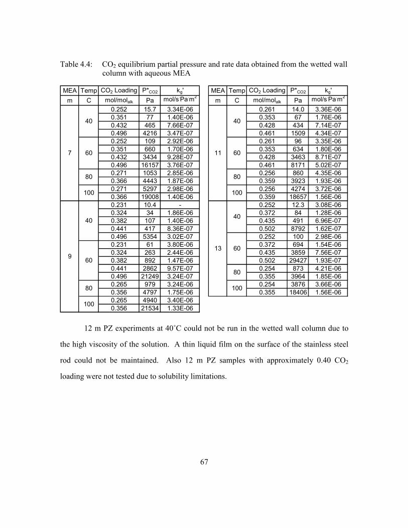
67

Table 4.4: CO2 equilibrium partial pressure and rate data obtained from the wetted wall column with aqueous MEA

MEA Temp CO2 Loading P*CO2 kg' MEA Temp CO2 Loading P*CO2 kg'

m C mol/molalk Pa mol/s.Pa

.m

2m C mol/molalk Pa mol/s

.Pa

.m

2

0.252 15.7 3.34E-06 0.261 14.0 3.36E-06

0.351 77 1.40E-06 0.353 67 1.76E-06

0.432 465 7.66E-07 0.428 434 7.14E-07

0.496 4216 3.47E-07 0.461 1509 4.34E-07

0.252 109 2.92E-06 0.261 96 3.35E-06

0.351 660 1.70E-06 0.353 634 1.80E-06

0.432 3434 9.28E-07 0.428 3463 8.71E-07

0.496 16157 3.76E-07 0.461 8171 5.02E-07

0.271 1053 2.85E-06 0.256 860 4.35E-06

0.366 4443 1.87E-06 0.359 3923 1.93E-06

0.271 5297 2.98E-06 0.256 4274 3.72E-06

0.366 19008 1.40E-06 0.359 18657 1.56E-06

0.231 10.4 - 0.252 12.3 3.08E-06

0.324 34 1.86E-06 0.372 84 1.28E-06

0.382 107 1.40E-06 0.435 491 6.96E-07

0.441 417 8.36E-07 0.502 8792 1.62E-07

0.496 5354 3.02E-07 0.252 100 2.98E-06

0.231 61 3.80E-06 0.372 694 1.54E-06

0.324 263 2.44E-06 0.435 3859 7.56E-07

0.382 892 1.47E-06 0.502 29427 1.93E-07

0.441 2862 9.57E-07 0.254 873 4.21E-06

0.496 21249 3.24E-07 0.355 3964 1.85E-06

0.265 979 3.24E-06 0.254 3876 3.66E-06

0.356 4797 1.75E-06 0.355 18406 1.56E-06

0.265 4940 3.40E-06

0.356 21534 1.33E-06

7

9

80

100

40

60

40

60

80

100

11

13

80

100

40

60

40

60

80

100

12 m PZ experiments at 40˚C could not be run in the wetted wall column due to

the high viscosity of the solution. A thin liquid film on the surface of the stainless steel

rod could not be maintained. Also 12 m PZ samples with approximately 0.40 CO2

loading were not tested due to solubility limitations.

68

Table 4.5: CO2 equilibrium partial pressure and rate data obtained from the wetted wall column with aqueous PZ

PZ Temp CO2 Loading P*CO2 kg' PZ Temp CO2 Loading P*CO2 kg'

m C mol/molalk Pa mol/s.Pa

.m

2m C mol/molalk Pa mol/s

.Pa

.m

2

0.240 96 3.32E-06 0.231 68 4.27E-06

0.316 499 2.04E-06 0.305 530 1.98E-06

0.352 1305 1.39E-06 0.360 1409 1.14E-06

0.411 7127 5.55E-07 0.404 8153 3.53E-07

0.240 559 3.33E-06 0.231 430 4.41E-06

0.316 2541 2.06E-06 0.305 2407 2.02E-06

0.352 5593 1.38E-06 0.360 7454 9.57E-07

0.411 25378 3.84E-07 0.404 30783 3.20E-07

0.239 2492 3.34E-06 0.253 3255 3.61E-06

0.324 12260 1.32E-06 0.289 9406 1.97E-06

0.239 9569 2.40E-06 0.253 13605 2.18E-06

0.324 39286 9.12E-07 0.289 32033 1.20E-06

0.226 65 4.39E-06 0.231 331 4.19E-06

0.299 346 2.57E-06 0.289 1865 1.85E-06

0.354 1120 1.69E-06 0.354 6791 7.73E-07

0.402 4563 7.93E-07 0.222 2115 4.24E-06

0.226 385 4.75E-06 0.290 9141 1.48E-06

0.299 1814 2.62E-06 0.222 7871 3.78E-06

0.354 5021 1.80E-06 0.290 33652 8.30E-07

0.402 17233 6.59E-07

0.238 2192 4.67E-06

0.321 9699 1.91E-06

0.238 8888 3.52E-06

0.321 36960 1.02E-06

60

2

5

80

100

80

100

40

60

40

40

60

60

8

12

80

100

80

100

Table 4.6: CO2 equilibrium partial pressure and rate data obtained from the wetted wall column with 7 m MEA/2 m PZ

MEA PZ Temp CO2 Ldg P*CO2 kg'

m m C mol/molalk Pa mol/s.Pa

.m

2

0.242 27 3.45E-06

0.333 166 1.96E-06

0.416 1425 8.76E-07

0.477 7418 4.32E-07

0.242 178 4.00E-06

0.333 1256 2.03E-06

0.416 7122 9.08E-07

0.477 33704 3.75E-07

0.242 1138 4.29E-06

0.333 6174 2.12E-06

0.242 4340 4.83E-06

0.333 26571 1.23E-06

7 2

40

60

80

100

69

4.4.2 Equilibrium CO2 Partial Pressure

The figures in the following sections graphically represent the data in Tables 4.4–

4.6 along with applicable literature data.

4.4.2.1 Monoethanolamine

Figure 4.2 shows CO2 equilibrium partial pressure values obtained from the

wetted wall column in 7, 9, 11, and 13 m MEA compared to Jou (1995) and Hilliard

(2008) values. Hilliard used an equilibrium cell to measure CO2 partial pressures with an

FTIR (Fourier transform infrared spectroscopy) analyzer to quantify the CO2

concentration. Jou also measured the equilibrium partial pressure with an equilibrium

cell.

1

10

100

1000

10000

100000

1000000

0.05 0.15 0.25 0.35 0.45 0.55

CO2 Loading (mol/molalk)

P* C

O2 (Pa)

Hilliard 3.5 m MEAHilliard 7 m MEAHilliard 11 m MEA7 m MEA9 m MEA11 m MEA13 m MEAJou 7 m MEA

Open Points – Hilliard (2008) – 3.5, 7, 11 m MEA

Dashes – Jou (1995) – 7 m MEA

Filled Points – Current Work – 7, 9, 11, 13 m MEA

100˚C

80˚C

60˚C

40˚C1

10

100

1000

10000

100000

1000000

0.05 0.15 0.25 0.35 0.45 0.55


P* C

O2 (Pa)





100˚C

80˚C

60˚C

40˚C

Figure 4.2: Equilibrium CO2 partial pressure measurements in MEA solutions at 40, 60, 80, and 100˚C (Jou, Mather et al. 1995; Hilliard 2008)

70

The 3.5, 7, and 11 m MEA data by Hilliard (2008), the 7 m MEA data by Jou

(1995) and the current work at 7, 9, 11, and 13 m MEA agree well at each of the four

temperatures. The current data represented by the filled data points show minor

deviations from the other data near 0.5 loading at 40˚C. The 0.5 loading data at 40 and

60˚C show an amine concentration dependence. At both 40 and 60˚C near 0.5 loading

the 13 m data has a higher CO2 partial pressure than the 11 m MEA data, which is higher

than the 7 m MEA data. The 11 m MEA data by Hilliard both at 40 and 60˚C also show

a higher CO2 partial pressure than 7 or 3.5 m MEA data at high CO2 loading. However,

the 7 m MEA, 0.5 loading, 40˚C measurement from the wetted wall column provides a

higher CO2 partial pressure value than the 7 m MEA data by Hilliard (2008) or Jou

(1995).

The effect of amine concentration on the CO2 partial pressure of the MEA system

at high loading is expected. Amine concentration should not affect CO2 equilibrium

partial pressures for carbamate-producing systems when compared at equivalent CO2

loading. However, amine concentration is extremely important in bicarbonate-producing

systems. MEA systems begin producing significant bicarbonate concentrations

approaching 0.5 loading. This difference is based on the stoichiometry of the carbamate

and bicarbonate reactions. The mathematics of the difference are explained in Appendix

D.

The increased CO2 partial pressure of the higher MEA concentrations near 0.5

loading is due to an increased concentration of bicarbonate. At lower CO2 loading,

bicarbonate concentration is insignificant and MEA concentration has no effect on the

equilibrium CO2 partial pressure of the system.

71

4.4.2.2 Piperazine

Figure 4.3 shows wetted wall column obtained CO2 equilibrium partial pressure

values in 2, 5, 8, and 12 m PZ compared to Ermatchkov (2006a) and Hilliard (2008).

Hilliard used an equilibrium cell to measure CO2 partial pressure with an FTIR (Fourier

transform infrared spectroscopy) analyzer to quantify the CO2 concentration.

Ermatchkov measured the equilibrium partial pressure using headspace gas

chromatography (2006b).

10

100

1000

10000

100000

0.10 0.15 0.20 0.25 0.30 0.35 0.40 0.45


P* C

O2 (Pa)

Hilliard 0.9 m PZ

Hilliard 2 m PZHilliard 2.5 m PZ

Hilliard 3.6 m PZ

Hilliard 5 m PZ8 m PZ

5 m PZ

12 m PZ2 m PZ

Ermatchkov 1-4.2 m PZ

Open Points – Hilliard (2008) – 0.9, 2, 2.5, 3.6, 5 m PZ

Dashes – Ermatchkov (2006) – 1-4.2 m PZ

Filled Points – Current Work – 2, 5, 8, 12 m PZ

100˚C

80˚C

60˚C

40˚C10

100

1000

10000

100000

0.10 0.15 0.20 0.25 0.30 0.35 0.40 0.45


P* C

O2 (Pa)

Hilliard 0.9 m PZ


Hilliard 3.6 m PZ


5 m PZ

12 m PZ2 m PZ





100˚C

80˚C

60˚C

40˚C

Figure 4.3: Equilibrium CO2 partial pressure measurements in PZ solutions at 40, 60, 80, and 100˚C (Ermatchkov, Perez-Salado Kamps et al. 2006a; Hilliard 2008)

All the data in Figure 4.3 match very well at 40, 60, and 80˚C. Neither

Ermatchkov (2006a) or Hilliard (2008) provide data at 100˚C but the 100˚C data are

72

reasonable based on the spacing from the 80˚C data and the overlap of the amine

concentrations.

Unlike the CO2 partial pressure measurements in the MEA system, the PZ system

does not show a dependence of amine concentration at high loading. This is because the

CO2 loading is not high enough to see appreciable quantities of bicarbonate. Since only

carbamates are produced, none of the data show an effect of amine concentration when

plotted against CO2 loading.

4.4.2.3 7 m MEA/2 m PZ

Little data for equilibrium CO2 partial pressure are available for

7 m MEA/ 2 m PZ. Figure 4.4 includes the current data (filled points) compared against

Hilliard (2008) represented as the open points. Hilliard used an equilibrium cell to

measure CO2 partial pressure with an FTIR analyzer to quantify the CO2 concentration.

73

1

10

100

1000

10000

100000

0.05 0.15 0.25 0.35 0.45


PCO2* (Pa)

Open Points – Hilliard (2008)

Filled Points – Current Work

100˚C

80˚C

60˚C

40˚C7 m MEA/2 m PZ

Figure 4.4: Equilibrium CO2 partial pressure measurements in 7 m MEA/2 m PZ at 40, 60, 80, and 100˚C (Hilliard 2008)

Although there are limited data for 7 m MEA/2 m PZ, the available equilibrium

CO2 partial pressure data show a very good match despite using two different

experimental apparatuses.

Other MEA/PZ concentrations were not studied due to concerns about thermal

degradation (Davis 2009). Davis found that the more reactive PZ will react preferentially

with an oxazolidone intermediate formed by thermally degrading MEA. Essentially, PZ

protects MEA from the thermal degradation of the blended system. PZ in the absence of

MEA will not thermally degrade significantly because there is no pathway to produce

oxazolidone.

74

4.4.3 CO2 Capacity

The equilibrium CO2 partial pressures in Figures 4.2–4.4, allow for the

determination of the CO2 capacity. The CO2 capacity is defined as the difference in the

CO2 concentration from the rich to the lean amine streams, not the total CO2

concentration in any particular stream. The CO2 capacity is the amount of CO2 that

would be removed from the system during one circulation of the amine solution.

The CO2 capacity is important because of energy tradeoffs of the sensible heat

and the heat of absorption. Circulating less solvent reduces the sensible heat duty since

the stripper must heat all the solution from the cross-exchanger outlet temperature to the

stripper temperature. This temperature difference is the same as the cross-exchanger

temperature approach. However, circulating too little solvent to achieve a high CO2

capacity requires a very low lean loading or CO2 partial pressure. Stripping to very low

CO2 partial pressures increases the stripping steam required per mole of CO2 and can

cause inefficient operation of the stripper. The optimal operating lean loading and thus

CO2 capacity for a given amine system requires a significant optimization with a complex

model. CO2 reaction rates change drastically with changing CO2 loading. Since the

optimal lean loading and thus CO2 partial pressure of that lean loading cannot be easily

determined, Figure 4.5 is constructed to compare the CO2 capacity of 8 m PZ and 7 and

13 m MEA at 40˚C for any lean partial pressure. Alternative amine systems allow for an

increase in the CO2 capacity of the system without requiring the system to strip to lower

CO2 partial pressures. Figure 4.5 includes CO2 loading values next to some of the data

points.

Since CO2 capacity relates to the sensible heat of the solution and the total

dissolved CO2 has a negligible partial heat capacity, CO2 capacities are calculated on a

75

molCO2/kg(water+amine) basis. It is not appropriate to include the CO2 in the weight of

the solution since it has a mostly negligible sensible heat. Essentially, a mole of MEA

has almost the same heat capacity as a mole of MEA carbamate (Hilliard 2008). Nguyen

has seen the same effect in PZ systems (Rochelle, Chen et al. 2009a).

0

0.5

1

1.5

2

2.5

101001000

CO

2 Capacity with a 5 kPa Rich Soln

(mol CO

2/kg(water+amine))

Lean Partial Pressure (Pa)

8 m PZ

7 m MEA.36 Ldg

.31

.23

.15 Ldg

.47

.31

.19

40C

.39

.54

.20

.30

.37

.49

11 m MEA

Figure 4.5: Operating CO2 capacity of 8 m PZ and 7 and 11 m MEA assuming a 5 kPa rich CO2 partial pressure at 40˚C (7 and 11 m MEA data from Hilliard (2008))

Figure 4.5 assumes a 5 kPa CO2 partial pressure rich solution. In a coal-fired

power plant CO2 enters the absorber near 12 mole%, or 12 kPa, since it is near

atmospheric pressure. Therefore, the assumption of a 5 kPa CO2 partial pressure rich

solution at 40˚C represents a 5/12 or a 42% approach to saturation at the bottom of the

absorber if the solution exits at 40˚C.

76

Under the assumed conditions detailed above, 8 m PZ exhibits about a 70%

greater CO2 capacity than 7 m MEA and about a 50% greater CO2 capacity than 11 m

MEA. The majority of the increased CO2 capacity is due to the fact that each mole of

piperazine has two functional nitrogen groups. This allows PZ to react with CO2 twice

while MEA can only react once. PZ solutions allow for much greater CO2 capacities than

MEA and thereby lower required liquid flow rates and the sensible heat input

requirement of the reboiler.

4.4.4 CO2 Reaction Rates

As explained in Section 2.3.1, CO2 absorption rates should be reported in terms of

kg’. The definition of kg’ is reiterated in Equation 4.5. kg’ is the liquid film mass transfer

coefficient converted to gas phase units.

)( *

,2,2

2'

bCOiCO

CO

gPP

Nk

−= (4.5)

Obtained kg’ values for each MEA experiment are plotted against the measured

equilibrium partial pressure at the temperature of the experiment in Figure 4.6. Figure

4.6 includes 7, 9, 11, and 13 m MEA rate data at 40, 60, 80, and 100˚C.

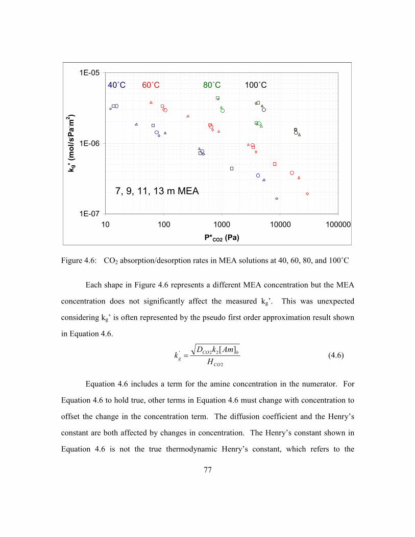
77

1E-07

1E-06

1E-05

10 100 1000 10000 100000

P*CO2 (Pa)

kg' (m

ol/s.Pa. m

2)

40˚C 60˚C 80˚C 100˚C

7, 9, 11, 13 m MEA

1E-07

1E-06

1E-05

10 100 1000 10000 100000

P*CO2 (Pa)

kg' (m

ol/s.Pa. m

2)

40˚C 60˚C 80˚C 100˚C

7, 9, 11, 13 m MEA

Figure 4.6: CO2 absorption/desorption rates in MEA solutions at 40, 60, 80, and 100˚C

Each shape in Figure 4.6 represents a different MEA concentration but the MEA

concentration does not significantly affect the measured kg’. This was unexpected

considering kg’ is often represented by the pseudo first order approximation result shown

in Equation 4.6.

2

22'][

CO

bCO

gH

AmkDk = (4.6)

Equation 4.6 includes a term for the amine concentration in the numerator. For

Equation 4.6 to hold true, other terms in Equation 4.6 must change with concentration to

offset the change in the concentration term. The diffusion coefficient and the Henry’s

constant are both affected by changes in concentration. The Henry’s constant shown in

Equation 4.6 is not the true thermodynamic Henry’s constant, which refers to the

78

solubility in water. The Henry’s constant shown in Equation 4.6 refers to the CO2

solubility in the solution. It is a function of amine concentration, CO2 loading, and

temperature (Browning and Weiland 1994; Hartono 2009).

The diffusion coefficient of CO2 will go down slightly with increasing MEA

concentration due to the viscosity effect. The CO2 solubility decreases (HCO2 increases)

with increasing amine concentration and this change cancels most of the increasing MEA

concentration term. Contrary to the data, Equation 4.6 does predict an amine

concentration effect on kg’.

Figure 4.6 seems to imply that kg’ in MEA solutions increases with increasing

temperature. However, that assertion is wrong. Rather than each increasing temperature

curve having a higher kg’, it has a higher CO2 equilibrium partial pressure. A close look

at Figure 4.6 reveals that kg’ is almost identical with increasing temperature. The 7 m

MEA (circles) data point at 40˚C near 15 Pa has a kg’ of approximately 3.3·10–6

mol/s.Pa

.m

2. The lowest loading data points for 7 m MEA at 60, 80, and 100˚C each

show a kg’ of approximately 3.0·10–6 mol/s

.Pa

.m

2. Each of these four data points has a

similar CO2 loading and kg’, verified in Table 4.4.

Since temperature has little effect on the measured kg’, the temperature dependent

terms in Equation 4.6 must cancel each other. The diffusion coefficient, rate constant,

and Henry’s constant are all temperature dependent. The diffusion coefficient will

decrease with increasing temperature due to viscosity changes. The rate constant will

increase with increasing temperature as shown by regressed literature data (Versteeg, Van

Dijck et al. 1996). The solubility of CO2 and N2O in water decreases with increasing

temperature (Versteeg and Van Swaaij 1988). Equation 4.6 does not predict kg’ to be

79

independent of temperature as the data indicate. Equation 4.6 is not supported by the

experimental data.

It would be convenient to show Figure 4.6 in terms of CO2 loading on the x-axis

but the CO2 loading basis would prohibit the MEA data from being compared to other

amines. Different amines can only be compared on a partial pressure basis since the

definition of CO2 loading is somewhat arbitrary and each amine has a different CO2

loading operating range. However, we can plot the x-axis in terms of the equilibrium

CO2 partial pressure at a given temperature. This results in two points with the same CO2

loading being plotted at the same value on the x-axis regardless of temperature. In this

respect it is similar to plotting the x-axis on a CO2 loading basis. However, this basis has

the advantage that it also allows a fair comparison of the CO2 reaction rates with different

amines. The equilibrium CO2 partial pressure at 40˚C can be viewed as a surrogate for

CO2 loading. The MEA rate data is plotted against the equilibrium CO2 partial pressure

at 40˚C in Figure 4.7.

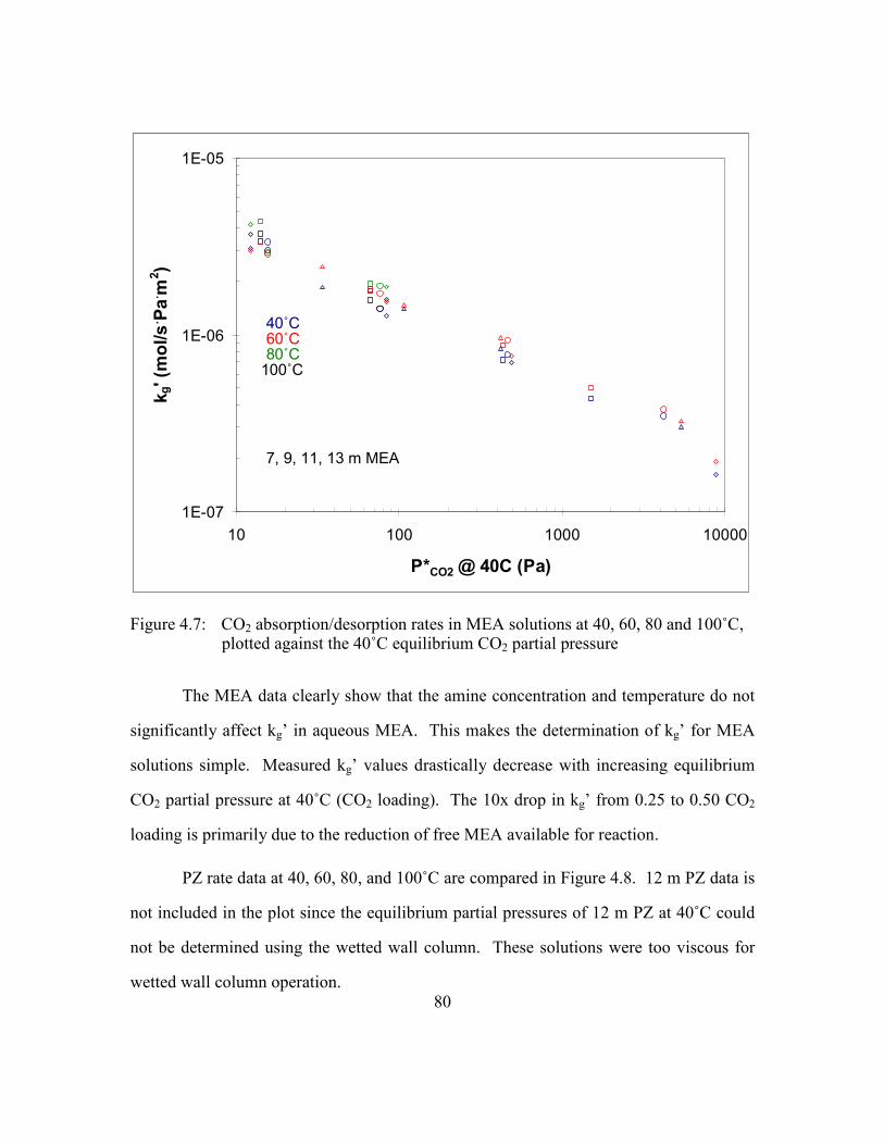
80

1E-07

1E-06

1E-05

10 100 1000 10000

P*CO2 @ 40C (Pa)

kg' (m

ol/s. Pa. m

2)

7, 9, 11, 13 m MEA

100˚C80˚C60˚C40˚C

1E-07

1E-06

1E-05

10 100 1000 10000

P*CO2 @ 40C (Pa)

kg' (m

ol/s. Pa. m

2)

7, 9, 11, 13 m MEA

100˚C80˚C60˚C40˚C

Figure 4.7: CO2 absorption/desorption rates in MEA solutions at 40, 60, 80 and 100˚C, plotted against the 40˚C equilibrium CO2 partial pressure

The MEA data clearly show that the amine concentration and temperature do not

significantly affect kg’ in aqueous MEA. This makes the determination of kg’ for MEA

solutions simple. Measured kg’ values drastically decrease with increasing equilibrium

CO2 partial pressure at 40˚C (CO2 loading). The 10x drop in kg’ from 0.25 to 0.50 CO2

loading is primarily due to the reduction of free MEA available for reaction.

PZ rate data at 40, 60, 80, and 100˚C are compared in Figure 4.8. 12 m PZ data is

not included in the plot since the equilibrium partial pressures of 12 m PZ at 40˚C could

not be determined using the wetted wall column. These solutions were too viscous for

wetted wall column operation.

81

1E-07

1E-06

1E-05

10 100 1000 10000

P*CO2 @ 40C (Pa)

kg' (m

ol/s. Pa. m

2)

2, 5, 8 PZ

100˚C80˚C60˚C40˚C

1E-07

1E-06

1E-05

10 100 1000 10000

P*CO2 @ 40C (Pa)

kg' (m

ol/s. Pa. m

2)

2, 5, 8 PZ

100˚C80˚C60˚C40˚C

Figure 4.8: CO2 absorption/desorption rates in PZ solutions at 40, 60, 80 and 100˚C, plotted against the 40˚C equilibrium CO2 partial pressure

The PZ data do not converge quite as cleanly as the MEA data. Measured kg’

values in aqueous PZ are not dependent on the amine concentration. However, there are

some temperature effects. At the lowest CO2 loading near 70–100 Pa, 100˚C data points

drop below the trend of the other data. At the next highest CO2 loading near 300–500 Pa,

80˚C data points drop from the trend while the 100˚C data points drop far below the

trend. At the two highest loadings only 40 and 60˚C data is available but the 60˚C data

points routinely fall below the 40˚C data points.

The observed temperature effects in the PZ data suggest that diffusion of products

and reactants may be limiting the reaction of the CO2 with the amine. At the lowest CO2

82

loading, there is adequate free amine at the interface and CO2 fluxes are small at the

lower temperatures. Tested CO2 partial pressures range from 0–2 times the equilibrium

partial pressure, not the equilibrium partial pressure at 40˚C. Therefore, fluxes at 100˚C

are very high compared to lower temperatures. It is possible that these fluxes combined

with fast CO2 reaction rates are depleting the interface of reactive PZ and PZ carbamate.

At the next highest loading, there is less free PZ carbamate at the interface while CO2

fluxes are higher due to the increased equilibrium partial pressure of the solutions. At

this loading, the 80˚C data are now being restrained by diffusion limitations while 100˚C

are hampered by the diffusion of reactants and products near the interface. At the higher

loadings, the PZ carbamate concentration continues to decrease while CO2 fluxes

continue to increase, thereby possibly slowing the measured mass transfer coefficients at

60˚C.

Although the PZ rate data suggest this diffusion limiting phenomenon, a model is

required to verify it. On the other hand, the MEA experiments do not suggest significant

mass transfer resistance due to the diffusion of reactants and products.

The proposed diffusion limitation in PZ experiments in the wetted wall column

may not be seen in industrial columns. The wetted wall column has a smaller liquid film

physical mass transfer coefficient, klo, than a typical industrial column. This is due to the

9.1 cm stainless steel contactor. In a packed industrial column, either structured or

random packing, the mean flow path of the solvent is probably closer to 2–3 cm. The

more frequent mixing of the solvent will refresh the interface and discourage depletion of

the reactants at the gas-liquid interface.

83

The MEA, PZ, and the MEA/PZ data are compared in Figure 4.9. MEA is

represented by the empty points. PZ is represented by the filled data points.

7 m MEA/2 m PZ data are marked with X’s.

1E-07

1E-06

1E-05

10 100 1000 10000

P*CO2 @ 40C (Pa)

kg' (mol/s. Pa. m

2)

Filled Points – 2, 5, 8 m PZ

Empty Points – 7, 9, 11, 13 m MEA

100˚C80˚C60˚C40˚C

X’s – 7 m MEA/2 m PZ

1E-07

1E-06

1E-05

10 100 1000 10000

P*CO2 @ 40C (Pa)

kg' (mol/s. Pa. m

2)

Filled Points – 2, 5, 8 m PZ

Empty Points – 7, 9, 11, 13 m MEA

100˚C80˚C60˚C40˚C

X’s – 7 m MEA/2 m PZ

Figure 4.9: CO2 absorption/desorption rates in MEA, PZ, and MEA/PZ solutions at 40, 60, 80, and 100˚C, plotted against the 40˚C equilibrium CO2 partial pressure

Most of the PZ data points form a trend line above the MEA data. These data

show that kg’ for PZ is 2–3 times faster than MEA. This means PZ reacts with CO2 2–3

times faster than MEA. To a first approximation 1/2 to 2/3 less packing in the absorber

would be required for PZ.

The 7 m MEA/2 m PZ rate data generally fall between the MEA and PZ data.

The condition near 200 Pa suggests diffusion limitations at the 100˚C condition.

84

4.4.4.1 Rate Comparisons with Literature

4.4.4.1.1 Monoethanolamine

Rate data obtained in this work are compared to literature values in this section.

As previously stated, there are limited rate data on highly loaded concentrated amines.

For a proper comparison on a kg’ basis, some raw data are required.

Figure 4.10 shows a comparison of 7 m MEA rate data at 40 and 60˚C.

Aboudheir (2003) provides rate data obtained from a laminar jet absorber. At each

condition multiple measurements were made. Figure 4.10 also includes four wetted wall

column data points obtained by Dang (2003). Dang used the same wetted wall column

used in this work. A single 40˚C data point from Hartono (2009) is included in Figure

4.10.

85

4x10-7

6x10-7

8x10-7

1x10-6

3x10-6

0 0.1 0.2 0.3 0.4 0.5

kg' (mol/s. Pa. m

2)

CO2 Loading (mol/mol)

7 m MEA

Circle - Harono (2009)

X's - Aboudheir (2003)

Squares - Dang (2003)

Triangles - Current Work

60C40C

Figure 4.10: CO2 reaction rate comparison on a kg’ basis for 7 m MEA at 40 and 60˚C (Aboudheir, Tontiwachwuthikul et al. 2003; Dang and Rochelle 2003; Hartono 2009)

The data by Dang coincide with the newly obtained wetted wall column data.

The data by Aboudheir also agree at the two higher CO2 loadings. The data by

Aboudheir (2003) near 0.1 loading show a lower kg’ value than an extrapolation of the

wetted wall column data would predict. However, the unloaded rate data by Hartono

(2009) support these 0.1 CO2 loading values and suggest that the liquid film mass transfer

coefficient, kg’, may not change significantly from 0 to 0.25 CO2 loading.

No wetted wall column experiments were conducted below 0.2 CO2 loading. The

wetted wall column cannot accurately obtain rate data in MEA solutions at CO2 loading

much lower than 0.25 because the system becomes dominated by the gas film mass

86

transfer coefficient. The gas film mass transfer coefficient of the column was originally

characterized using unloaded MEA (Pacheco 1998).

The data by Aboudheir (2003) show a consistent effect of temperature. In each of

the three CO2 loadings, the 60˚C data points exhibit about 50% higher kg’ values. The

wetted wall column data, including Dang (2003) and the current work, do not clearly

show a trend. Figure 4.7 more clearly shows that there is no significant temperature

effect on the CO2 absorption/desorption rates in MEA solutions. The wetted wall column

apparatus used in the current work and by Dang (2003) is very different from the laminar

jet absorber used by Aboudheir (2003).

Unloaded MEA rate data found in the literature could also be compared to the

highly loaded, highly concentrated MEA rate data presented here. As the Literature

Review detailed, there are numerous sources which report rate data in unloaded,

relatively dilute MEA solutions. However, most of these data sources only report

obtained rate constants and do not detail values used for the Henry’s constant or the

diffusion coefficient. Neither do they include fluxes and driving forces which allow for

the calculation of kg’.

Laddha and Danckwerts (1981a) provide calculated rate constants along with the

solubility and diffusion parameters that allow for the calculation of the measured flux and

KG. No gas film mass transfer coefficients were given for the stirred cell experiments so

kg’ cannot be calculated. The rate constants (expressed in Equation 4.7) for the six tested

amine concentrations ranged from 5.49 to 6.28 m3/(mol

.s) at 25˚C (Laddha and

Danckwerts 1981a). These rate constants compare favorably with 5.99 m3/(mol

.s) value

predicted by a correlation developed from a review of literature data (Versteeg, Van

Dijck et al. 1996).

87

[ ][ ]222 COMEAkrCO =− (4.7)

Hartono (2009) provides all the important experimental data from his CO2

absorption into MEA. This allows for the calculation of KG and then kg’. The rate

experiments performed using a string of discs were determined to be 5–18% gas film

controlled. The calculated kg’ from the experiments by Hartono (2009) and the

calculated KG values from Laddha (1981a) are shown in Figure 4.11.

7x10-7

8x10-7

9x10-7

1x10-6

2x10-6

3x10-6

4x10-6

0 1 2 3 4 5

KG or kg' (mol/s. Pa. m

2)

MEA Concentration (Molarity)

25C

25C

30C

40C

50CKG - Laddha and Danckwerts (1981)

kg' - Hartono (2009)

Figure 4.11: CO2 reaction rates in unloaded MEA solutions (Laddha and Danckwerts 1981a; Hartono 2009)

Figure 4.11 shows the Laddha data at 25˚C below the Hartono data at 25˚C. This

is expected since the Laddha data do not remove the gas film resistance from the system.

The liquid film mass transfer coefficient, kg’, must be larger than the overall mass

transfer coefficient, KG. In cases where the gas film mass transfer coefficient, kg, is

limiting, KG can be significantly lower than kg’. In a stirred cell experiment with

88

unloaded MEA, it is likely that gas film mass transfer resistance is significant since

stirred cells often have this concern. The Laddha data in Figure 4.11 are not as

descriptive of CO2 rates into MEA as the Hartono data. Gas film resistances due to

operating conditions and the geometry of the apparatus cannot be extracted from the

reported data.

Figure 4.11 shows a dependence of kg’ on the MEA concentration at lower MEA

concentrations. At higher MEA concentrations kg’ becomes independent of

concentration, although at different amine concentrations for different temperatures. This

independence of concentration on kg’ is also seen in the current MEA rate data (Figure

4.7) which was taken at high MEA concentrations.

4.4.4.1.2 Piperazine

Although Table 2.2 of the Literature Review only lists 5 references for CO2

reaction rates into aqueous PZ solutions, all provide some raw experimental data. Sun

(2005), Derks (2006), Cullinane (2006), and Samanta (2007) include unloaded PZ rate

data while Bishnoi (2000) provides CO2 loaded rate data. All five data sources use low

piperazine concentrations.

Derks uses a stirred cell and a “semi-continuous” gas phase operation. Numerous

CO2 partial pressures were tested for each amine to determine when the pseudo first order

condition applies. At high CO2 partial pressures, diffusion in the liquid phase limits CO2

mass transfer. For 1.0 M PZ at 40˚C, approximately 1.5 kPa CO2 was the threshold for

the onset of the pseudo first order condition. Inlet CO2 partial pressures above 1.5 kPa

showed a distinct effect of the partial pressure on the measured KG. Below the threshold,

the overall mass transfer coefficient is independent of the inlet partial pressure.

89

Sun (2005) and Samanta (2007) each measured the absorption into unloaded PZ

solutions using wetted wall columns. Each used very high CO2 partial pressures,

typically about 5 kPa. At these high CO2 partial pressures and amine concentrations

below 1 M, CO2 fluxes into the liquid phase should be restricted by diffusion. In fact,

Sun (2005) tested a few lower CO2 partial pressures and these data verify that the system

is not operating in the pseudo first order regime at the 5 kPa CO2 pressure experiments,

which comprise most of the data. Although we cannot extract a meaningful kg’ value

from these raw data, they can still be valuable. These data require a model to account for

the diffusion limitations in the system.

Cullinane provides all the required data to calculate kg’. At each condition, five

measurements were made. Obtained kg’ values were shown to range ± 30% from the

mean due to the high dependence on the gas film mass transfer coefficient. The 1.2 m PZ

experiments were 54–73% gas film controlled. Only 25 and 60˚C experiments were

tested. The Cullinane experiments all use very low CO2 partial pressures (< 250 Pa) so

the pseudo first order condition should apply.

Figure 4.12 shows a comparison of the obtained 2 m PZ wetted wall column rate

data with some literature obtained values. Figure 4.12 includes an unloaded 1.0 M PZ

data point from Derks. This point is actually the obtained overall mass transfer, KG, not

the liquid film mass transfer coefficient, kg’. Derks does not provide a gas film mass

transfer coefficient correlation to quantify if or how much gas phase resistance limits CO2

absorption into the solution. For purposes of comparison, the KG obtained from Derks is

plotted alongside the kg’ data and the kg’ model prediction from Cullinane (2005).

90

6x10-7

8x10-7

1x10-6

3x10-6

5x10-6

7x10-6

0 0.1 0.2 0.3 0.4

kg' (mol/s. Pa. m

2)

CO2 Loading (mol/mol

alk)

Triangle - Derks (2006) (KG)1.0 M PZ

Squares - Bishnoi (2000) 0.06-0.31 m PZLine - Cullinane (2005) 1.8 m PZ Model Prediction

X's - Cullinane (2006) 1.2 m PZ (25 and 60C)Circles - Current Work 2 m PZ

40C

PZ60C

25C

Figure 4.12: CO2 reaction rate comparison on a kg’ basis for aqueous PZ at 40˚C (Bishnoi and Rochelle 2000; Cullinane 2005; Cullinane and Rochelle 2006; Derks, Kleingeld et al. 2006)

Figure 4.12 shows good agreement of the current 2 m PZ rate data with the 1.8 m

PZ model prediction by Cullinane (2005). The loaded Bishnoi data shows mass transfer

coefficients below the current data. This is expected due to the very low PZ

concentration (0.06–0.31 m PZ) in these experiments. Interestingly, these data show the

same trend as the 2 m PZ data. Very low amine concentrations also exhibited a reduced

kg’ in MEA solutions (Figure 4.11).

The unloaded data in Figure 4.12 are difficult to analyze. Similar to the MEA

data by Hartono (2009), the 25 and 60˚C data points by Cullinane show a significant

temperature effect at 0 loading. These 1.2 m PZ data points show an acceptable fit to the

91

1.8 m 40˚C model prediction. The Derks overall mass transfer coefficient falls

significantly below the other unloaded data, which was not unexpected. This suggests

that the gas film mass transfer coefficient is likely limiting mass transfer into the PZ

solution. The limitation of the gas film mass transfer coefficient is a disadvantage of

using stirred cell reactors to measure CO2 reaction rates of very fast amines.

4.5 DESIGN OF AN ISOTHERMAL ABSORBER

A large amount of rate and equilibrium data has been produced this chapter. This

section indicates how the data can be used to design an isothermal absorber.

4.5.1 Design Basis

This example assumes 90% CO2 removal of a 500 MW power plant with 12%

CO2 in the flue gas. A 500 MW power plant produces approximately 25 kmol/s of flue

gas. The solvent is 8 m PZ with lean a rich partial pressures of 0.5 and 5.0 kPa at 40˚C.

These partial pressures correspond to 0.31 lean loading and 0.41 rich loading. The

isothermal absorber operates at 40˚C. This system is assumed to operate in the pseudo

first order regime so the diffusion of reactants and products to and from the reaction

interface is unimportant.

4.5.2 Calculations

The first step in the calculations is to determine the CO2 flux at the top and

bottom of the absorber. A log mean average of the two fluxes provides an average flux

of the column. Figure 4.8 or Table 4.5 provide values for kg’.

( )leanCOtopCOCldgmPZgtopCO PPkFlux ,,40,31.0,8

'

, 222−= (4.8)

( )2

3

2

6

,22

2104.15001200102

ms

molPaPa

mPas

molFlux

COCO

topCO ⋅⋅=−

⋅⋅⋅= −− (4.9)

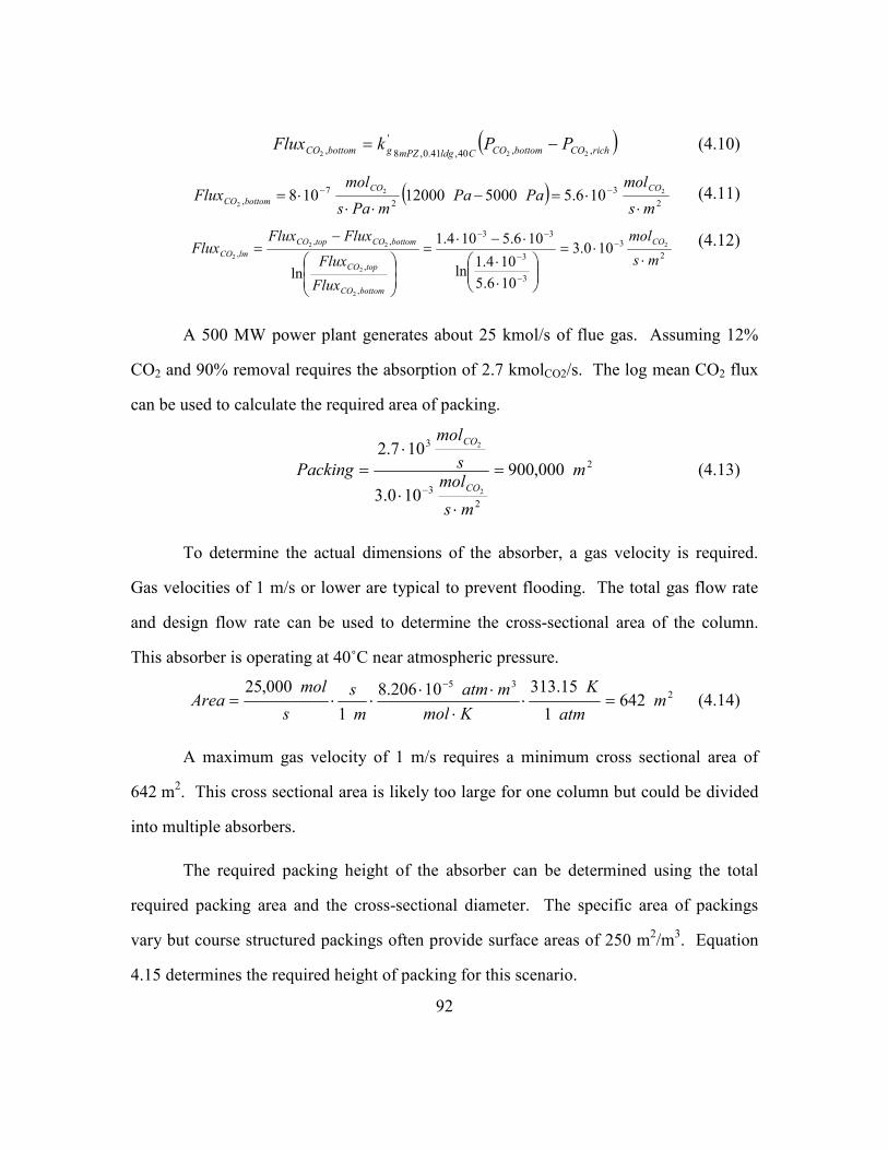
92

( )richCObottomCOCldgmPZgbottomCO PPkFlux ,,40,41.0,8

'

, 222−= (4.10)

( )2

3

2

7

,

22

2106.5500012000108

ms

molPaPa

mPas

molFlux

COCO

bottomCO⋅

⋅=−⋅⋅

⋅= −− (4.11)

2

3

3

3

33

,

,

,,

,2

2

2

22

2100.3

106.5

104.1ln

106.5104.1

lnms

mol

Flux

Flux

FluxFluxFlux

CO

bottomCO

topCO

bottomCOtopCO

lmCO ⋅⋅=

⋅

⋅

⋅−⋅=

−= −

−

−

−− (4.12)

A 500 MW power plant generates about 25 kmol/s of flue gas. Assuming 12%

CO2 and 90% removal requires the absorption of 2.7 kmolCO2/s. The log mean CO2 flux

can be used to calculate the required area of packing.

2

2

3

3

000,900

100.3

107.2

2

2

m

ms

mols

mol

PackingCO

CO

=

⋅⋅

⋅=

−

(4.13)

To determine the actual dimensions of the absorber, a gas velocity is required.

Gas velocities of 1 m/s or lower are typical to prevent flooding. The total gas flow rate

and design flow rate can be used to determine the cross-sectional area of the column.

This absorber is operating at 40˚C near atmospheric pressure.

235

6421

15.31310206.8

1

000,25m

atm

K

Kmol

matm

m

s

s

molArea =⋅

⋅⋅⋅

⋅⋅=−

(4.14)

A maximum gas velocity of 1 m/s requires a minimum cross sectional area of

642 m2. This cross sectional area is likely too large for one column but could be divided

into multiple absorbers.

The required packing height of the absorber can be determined using the total

required packing area and the cross-sectional diameter. The specific area of packings

vary but course structured packings often provide surface areas of 250 m2/m

3. Equation

4.15 determines the required height of packing for this scenario.

93

mmm

mmHeight 6.5

642

1

250000,900

22

32 =⋅⋅= (4.15)

4.5.3 Analysis

This design is not optimal. However, it does show the methodology for sizing an

absorber using data presented in this work. This analysis uses only the top and bottom of

the absorber to determine the average CO2 flux. Including intermediate points would

greatly increase the accuracy of the analysis.

If CO2 concentration in the gas phase is assumed to change linearly in the

absorber as a function of absorber height, the CO2 loading must also change linearly to

satisfy the CO2 material balance. A linear change in CO2 loading produces an

exponential change in the equilibrium CO2 partial pressure of the solution. This

exponential change causes the largest CO2 fluxes to be observed in the interior of an

isothermal absorber. Therefore, using just the top and bottom of the absorber to

determine the average CO2 flux is not recommended.

94

Chapter 5: Modeling

5.1 SPREADSHEET MODELING

As Section 2.2.3 on film theory shows, the liquid film mass transfer coefficient,

kg’, results from both reaction and diffusion resistances. These resistances in the liquid

film can be separated using a series resistance.

[ ]

∆

∆+=

T

o

ggCO

P

kkk

CO

prodl 2

*

'''

2

,

111 (5.1)

In Equation 5.1, the first term refers to the reaction resistance which is

characterized by the pseudo first order condition. The second term represents diffusion

resistance and incorporates the slope of the equilibrium line and the physical mass

transfer coefficient of the reactants and products.

An analytical expression to calculate kg’ at highly concentrated, highly loaded

conditions has previously remained elusive and thus required experimentation to

determine CO2 mass transfer rates. This approach attempts to identify and re-evaluate the

assumptions in the typical treatment of calculating kg’.

The reaction portion of Equation 5.1 requires the reaction rate of CO2. This can

be defined generically by Equation 5.2 in which the order of the reaction with respect to

the amine is variable. The value of “x” will be determined by evaluating experimental

data.

[ ] [ ] [ ]( )eCO

xx

AmCO COCOAmkr 2222 −−= γγ (5.2)

95

Solving the material balance and using the proper boundary conditions with the

pseudo first order assumption produces in Equation 5.3, which is more complex than the

traditional expression (Equation 2.30).

OHCOCO

CO

xx

Am

gH

DAmkk

2,2

5.0

2

2''][

γ

γ= (5.3)

The more complex expression requires an understanding of the rate constant, the

activity coefficients of both the amine and CO2, the order of the amine, and the diffusion

coefficient of CO2. Equation 5.3 can only represent the reaction resistance.

Experimental conditions with significant diffusion resistances also require an accurate

representation of the slope of the equilibrium line and the mass transfer coefficient of the

products and reactants. All of the varying parameters for both monoethanolamine and

piperazine are explored in the following sections. Equation 5.4 combines Equations 5.1

and 5.3 to list the generic expression for calculating kg’.

[ ]

∆

∆+=

T

o

CO

xx

Am

OHCOCO

gCO

P

kDAmk

H

k

CO

prodl 2

*

2

2,2

5.0

2

'

2

,

1

][

1

γ

γ (5.4)

Appendix F includes results of the MEA and PZ spreadsheet models.

5.1.1 Monoethanolamine Systems

5.1.1.1 Activity Coefficients

The rate expression is determined by the activity of the reactants, not the

concentration of the reactants. It cannot be assumed that activity coefficients are near 1.0

in highly loaded, highly concentrated MEA solutions. These solutions are highly ionic

and should be treated thus.

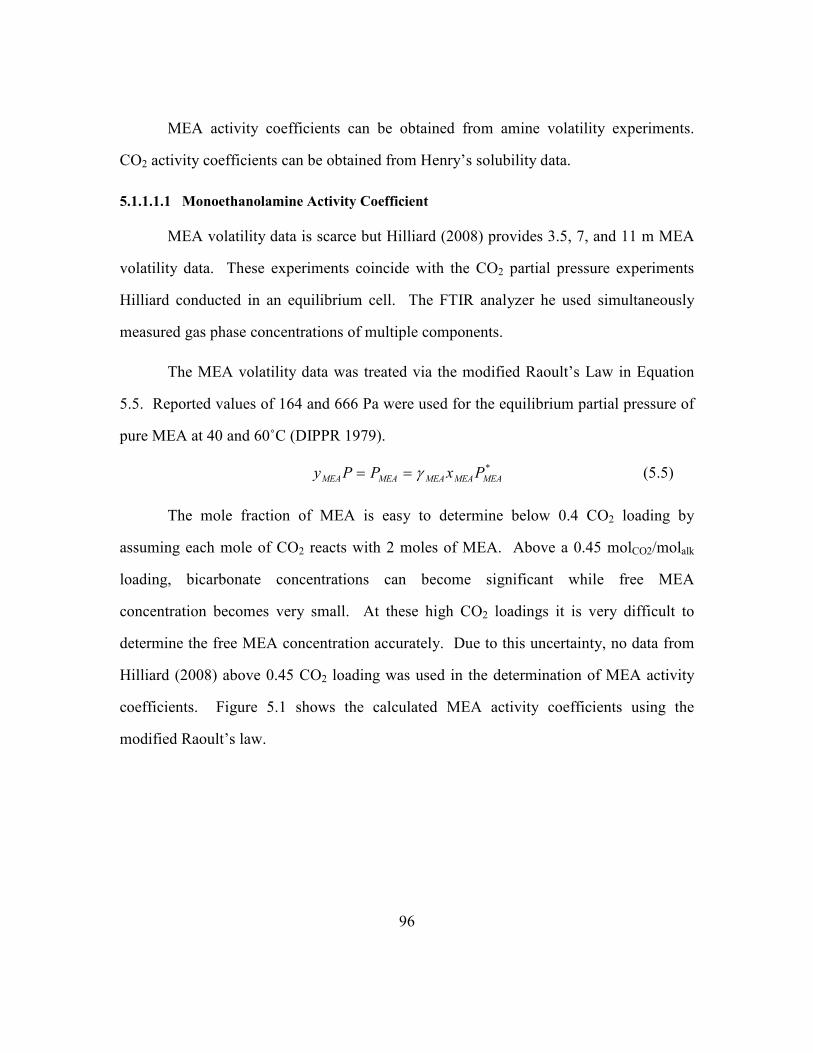
96

MEA activity coefficients can be obtained from amine volatility experiments.

CO2 activity coefficients can be obtained from Henry’s solubility data.

5.1.1.1.1 Monoethanolamine Activity Coefficient

MEA volatility data is scarce but Hilliard (2008) provides 3.5, 7, and 11 m MEA

volatility data. These experiments coincide with the CO2 partial pressure experiments

Hilliard conducted in an equilibrium cell. The FTIR analyzer he used simultaneously

measured gas phase concentrations of multiple components.

The MEA volatility data was treated via the modified Raoult’s Law in Equation

5.5. Reported values of 164 and 666 Pa were used for the equilibrium partial pressure of

pure MEA at 40 and 60˚C (DIPPR 1979).

*

MEAMEAMEAMEAMEA PxPPy γ== (5.5)

The mole fraction of MEA is easy to determine below 0.4 CO2 loading by

assuming each mole of CO2 reacts with 2 moles of MEA. Above a 0.45 molCO2/molalk

loading, bicarbonate concentrations can become significant while free MEA

concentration becomes very small. At these high CO2 loadings it is very difficult to

determine the free MEA concentration accurately. Due to this uncertainty, no data from

Hilliard (2008) above 0.45 CO2 loading was used in the determination of MEA activity

coefficients. Figure 5.1 shows the calculated MEA activity coefficients using the

modified Raoult’s law.

97

0.2

0.4

0.6

0.8

1.0

0.10 0.15 0.20 0.25 0.30 0.35 0.40 0.45


MEA Activity Coefficient

7 m MEA, 40C 7 m MEA, 60C

11 m MEA, 40C 11 m MEA, 60C

3.5 m MEA, 40C 3.5 m MEA, 60C

Figure 5.1: Calculated MEA activity coefficients for 3.5, 7, and 11 m MEA at 40 and 60˚C (Hilliard 2008).

The Hilliard data show an increasing MEA activity coefficient with increased

CO2 loading. The MEA activity coefficient is also a function of temperature, with higher

temperatures having lower activity coefficients. Amine concentration is not major factor

in the determination of the activity coefficient. The 3.5, 7, and 11 m MEA data sets tend

to overlap.

The data in Figure 5.1 were regressed to produce an expression for the MEA

activity coefficient. The expression in Equation 5.6 is plotted as lines in Figure 5.2 to

show regressed values at 40, 60, 80, and 100˚C. Equation 5.6 expresses CO2 loading in

terms of mol/molalk and temperature in Kelvin.

( )T

LoadingCOMEA

150374.171.5ln 2 ++−=γ (5.6)

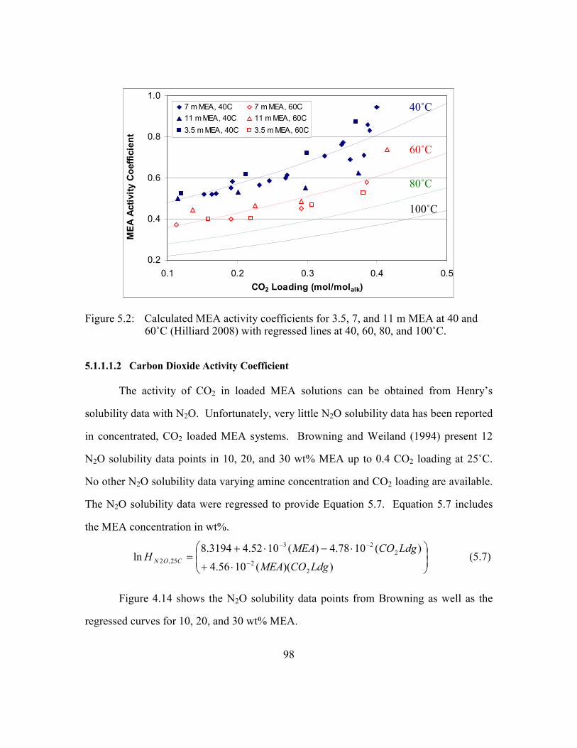
98

0.2

0.4

0.6

0.8

1.0

0.1 0.2 0.3 0.4 0.5



7 m MEA, 40C 7 m MEA, 60C

11 m MEA, 40C 11 m MEA, 60C

3.5 m MEA, 40C 3.5 m MEA, 60C

Figure 5.2: Calculated MEA activity coefficients for 3.5, 7, and 11 m MEA at 40 and 60˚C (Hilliard 2008) with regressed lines at 40, 60, 80, and 100˚C.

5.1.1.1.2 Carbon Dioxide Activity Coefficient

The activity of CO2 in loaded MEA solutions can be obtained from Henry’s

solubility data with N2O. Unfortunately, very little N2O solubility data has been reported

in concentrated, CO2 loaded MEA systems. Browning and Weiland (1994) present 12

N2O solubility data points in 10, 20, and 30 wt% MEA up to 0.4 CO2 loading at 25˚C.

No other N2O solubility data varying amine concentration and CO2 loading are available.

The N2O solubility data were regressed to provide Equation 5.7. Equation 5.7 includes

the MEA concentration in wt%.

⋅+

⋅−⋅+=

−

−−

))((1056.4

)(1078.4)(1052.43194.8ln

2

2

2

23

25,2LdgCOMEA

LdgCOMEAH CON (5.7)

Figure 4.14 shows the N2O solubility data points from Browning as well as the

regressed curves for 10, 20, and 30 wt% MEA.

80˚C

100˚C

60˚C

40˚C

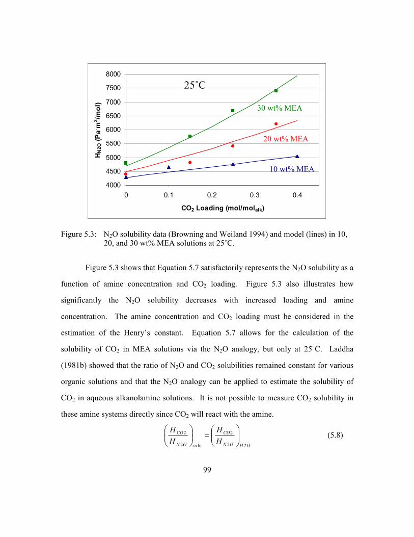
99

4000

4500

5000

5500

6000

6500

7000

7500

8000

0 0.1 0.2 0.3 0.4


HN2O (Pa. m

3/m

ol)

Figure 5.3: N2O solubility data (Browning and Weiland 1994) and model (lines) in 10, 20, and 30 wt% MEA solutions at 25˚C.

Figure 5.3 shows that Equation 5.7 satisfactorily represents the N2O solubility as a

function of amine concentration and CO2 loading. Figure 5.3 also illustrates how

significantly the N2O solubility decreases with increased loading and amine

concentration. The amine concentration and CO2 loading must be considered in the

estimation of the Henry’s constant. Equation 5.7 allows for the calculation of the

solubility of CO2 in MEA solutions via the N2O analogy, but only at 25˚C. Laddha

(1981b) showed that the ratio of N2O and CO2 solubilities remained constant for various

organic solutions and that the N2O analogy can be applied to estimate the solubility of

CO2 in aqueous alkanolamine solutions. It is not possible to measure CO2 solubility in

these amine systems directly since CO2 will react with the amine.

OHON

CO

soON

CO

H

H

H

H

22

2

ln2

2

=

(5.8)

10 wt% MEA

30 wt% MEA

20 wt% MEA

25˚C

100

The CO2 and N2O solubility data in water as a function of temperature have been

compiled and regressed (Versteeg and Van Swaaij 1988).

136

2,2 )/2044exp(1082.2 −⋅−⋅= molmPaTH OHCO (5.9)

136

2,2 )/2284exp(1055.8 −⋅−⋅= molmPaTH OHON (5.10)

Hartono (2009) recently published N2O solubility data in loaded 30 wt% (7 m)

MEA solutions. Hartono measured N2O solubility from 25–87˚C for 0, 0.2, 0.4, and 0.5

CO2 loading solutions. Figure 5.4 illustrates the N2O solubility results for each of the 4

CO2 loadings.

8

8.5

9

9.5

10

10.5

0.0027 0.0029 0.0031 0.0033

1/Temp (1/K)

ln (HN2O) (Pa. m

3/mol)

Figure 5.4: N2O solubility data (points) and trend lines for 0, 0.2, 0.4, and 0.5 CO2 loaded 7 m MEA (Hartono 2009)

The natural log of the N2O solubility plotted against inverse temperature yields

straight lines for each of the four CO2 loadings. The slope of the lines corresponds to the

temperature behavior of N2O solubility in 7 m MEA. The slopes of the four lines are

approximately equal with an average value of –1905/T. The N2O solubility temperature

effect in loaded MEA solutions can be added to Equation 5.7, which is only valid at

0.5 CO2 Loading

0.4 0.2 0

7 m MEA

101

25˚C. Equation 5.11 should be valid from 25 to at least 87˚C, the temperature range of

the regressed data.

−−

⋅+

⋅−⋅+=

−

−−

15.298

111905

))((1056.4

)(1078.4)(1052.43194.8exp

2

2

2

23

2TLdgCOMEA

LdgCOMEAH ON

(5.11)

Similar to the N2O solubility from Browning (1994), Hartono shows the N2O

solubility decreasing with increasing CO2 loading. Unfortunately, the data do not agree

completely. Both Hartono and Browning measure N2O solubility at 25˚C for 7 m MEA.

Figure 5.5 shows the disagreement between the two data sets.

4500

5000

5500

6000

6500

7000

7500

8000

0 0.1 0.2 0.3 0.4 0.5

CO2 Loading (mol/mol)

HN2O (kPa. L/mol)

Figure 5.5: N2O solubility in 7 m MEA at 25˚C (Browning and Weiland 1994; Hartono 2009)

Since these are the only two data sets for N2O solubility in loaded MEA solutions,

it is not possible to tell which data set is erroneous. In this work the Browning (1994)

data set has been used to quantify the effects of CO2 loading and MEA concentration on

7 m MEA

Circles Browning (1994)

Diamonds Hartono (2009)

25˚C

102

N2O solubility. The Hartono (2009) data set has been used to quantify the effect of

temperature on N2O solubility.

The calculation of the Henry’s constant of CO2 allows for the determination of the

activity coefficient of CO2 using Equation 5.12. The activity coefficient of CO2 is

assumed to be equivalent to the activity coefficient of N2O.

2

2,2

,2

2,20

2

2 CO

OHCO

CO

OHN

ON

ONH

H

H

Hγγ ===

(5.12)

HCO2 gives the effective solubility of CO2 in the solution. HCO2,H2O is the true

thermodynamic Henry’s constant, which refers to the solubility of CO2 in pure water.

The activity coefficient of CO2 varies between 1.3 and 3.2 for 7–13 m MEA wetted wall

column experiments.

5.1.1.2 Diffusion Coefficient of CO2

Work by Versteeg and Van Swaaij (1988) has shown that the diffusion of N2O

and CO2 in aqueous amines generally follows the viscosity dependence in Equation 5.13.

( ) ( )WaterONsoON DCONSTANTD 8.0

2ln

8.0

2 ηη == (5.13)

The N2O and CO2 diffusivity relationship in Equation 5.13 was confirmed with

MDEA solutions but resulted in less reliable results for AMP (Tomcej and Otto 1989;

Xu, Otto et al. 1991).

Diaphragm cell experiments in loaded MEA and PZ solutions yield a viscosity

dependence of 0.72 with a standard error of 0.12 (Figure 4.1). Although the 0.72

dependence obtained from the diaphragm cell experiments does not necessarily represent

CO2 diffusion, or diffusion of any other specific species, the 0.72 dependence was used

for calculation of the diffusion coefficient of CO2.

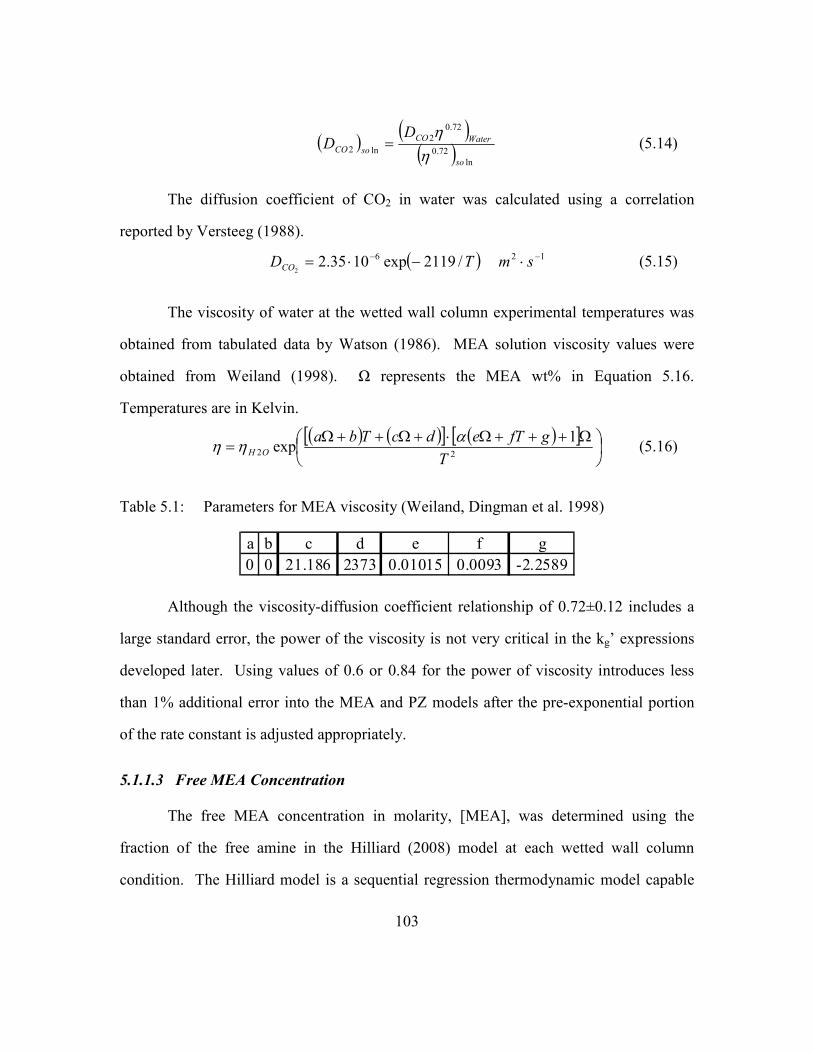
103

( ) ( )( ) ln

72.0

72.0

2

ln2

so

WaterCO

soCO

DD

η

η= (5.14)

The diffusion coefficient of CO2 in water was calculated using a correlation

reported by Versteeg (1988).

( ) 126 /2119exp1035.22

−− ⋅−⋅= smTDCO (5.15)

The viscosity of water at the wetted wall column experimental temperatures was

obtained from tabulated data by Watson (1986). MEA solution viscosity values were

obtained from Weiland (1998). Ω represents the MEA wt% in Equation 5.16.

Temperatures are in Kelvin.

( ) ( )[ ] ( )[ ]

Ω+++Ω⋅+Ω++Ω=

22

1exp

T

gfTedcTbaOH

αηη (5.16)

Table 5.1: Parameters for MEA viscosity (Weiland, Dingman et al. 1998)

a b c d e f g

0 0 21.186 2373 0.01015 0.0093 -2.2589

Although the viscosity-diffusion coefficient relationship of 0.72±0.12 includes a

large standard error, the power of the viscosity is not very critical in the kg’ expressions

developed later. Using values of 0.6 or 0.84 for the power of viscosity introduces less

than 1% additional error into the MEA and PZ models after the pre-exponential portion

of the rate constant is adjusted appropriately.

5.1.1.3 Free MEA Concentration

The free MEA concentration in molarity, [MEA], was determined using the

fraction of the free amine in the Hilliard (2008) model at each wetted wall column

condition. The Hilliard model is a sequential regression thermodynamic model capable

104

of handling systems containing H2O, CO2, MEA, PZ, and K+. Required density data

were obtained from the Weiland (1998) density correlation for MEA solutions.

V

MxMxMx COCOOHOHAmAm 2222++

=ρ (5.17)

***

222222VxxVxxVxVxVxV COAmOHAmCOCOOHOHAmAm ++++= (5.18)

cbTaT

MV Am

Am ++=

2 (5.19)

AmxedV ⋅+=** (5.20)

Table 5.2: Parameters for MEA density (Weiland, Dingman et al. 1998)

a b c d e MAm VCO2V*

-5.35162E-07 -4.51417E-04 1.19451 0 0 61.09 0.04747 -1.8218

5.1.1.4 Monoethanolamine Order

With estimations for the activity coefficients of MEA and CO2, the MEA

concentration dependence on kg’ can be examined. The rate data show a second order

dependence on the MEA concentration. This second order dependence can be satisfied

from either the zwitterion or termolecular mechanism, although the termolecular

mechanism is more likely for MEA. The termolecular mechanism allows for the

following base catalysis reaction expression.

[ ] [ ]( ) [ ] [ ]2222 COMEAOHkMEAkr OHMEACO ⋅⋅+−= (5.21)

For the second order dependence to be observed [ ]MEAkMEA must be much

greater than [ ]OHk OH 22 . Crooks and Donnellan (1989) report kMEA and kH2O values

based on 0.02–0.06 M MEA rate data. They report kMEA values about 2200 times larger

than kH2O. Bronsted theory, which relates base pKa’s to rate constants, would also

predict a kMEA value orders of magnitude larger than kH2O. If kMEA is 2200 times larger

105

than kH2O, more than 99% of the amine in 7 m MEA would have to be reacted before

water catalysis becomes significant. In this analysis with high MEA concentrations,

water catalysis has been ignored.

Density function theory calculations have also shown that water catalysis of the

zwitterion species is thermodynamically implausible due to an increase of energy in the

water catalyzed products (Shim, Kim et al. 2009). MEA catalyzed products were shown

to have a favorable decrease in energy compared to the zwitterion species.

In order for the second order amine dependence to match the zwitterion

mechanism, rk must be much greater than [ ]∑ Bkb in Equation 5.22, yielding Equation

5.23. This is not accepted for MEA (Danckwerts 1979) and is even more unlikely at high

MEA (base) concentrations tested in the wetted wall column.

∑+

−=

][

1

]][[ 2

2

Bkk

k

k

COAmr

bf

r

f

CO (5.22)

[ ][ ]∑−= ][22 BkCOMEAk

kr b

r

f

CO

(5.23)

The equations of this section have been written with respect to concentration for

simplicity. However, the model is activity-based, so activity coefficients can be inputted

into all the equations.

The majority of the literature data on MEA rates report kinetics with a first order

MEA dependence. These data are generally unloaded and at dilute MEA concentrations

using concentration-based kinetics. Concentrated MEA rate experiments evaluated using

concentration based kinetics have shown a greater than 1.0 dependence on the MEA

concentration (Aboudheir, Tontiwachwuthikul et al. 2003). Therefore, it is not

106

unrealistic to observe second order MEA kinetics for highly loaded, concentrated MEA

using activity-based kinetics.

5.1.1.5 Liquid Phase Mass Transfer Coefficient of Reactants and Products, 0

, prodlk

The liquid phase mass transfer coefficient of the reactants and products, 0

, prodlk ,

was calculated as shown in Section 3.2.2.2. Since the reactants and products are limiting,

the diffusion coefficient of the reactants and products must be incorporated.

2/1

6/13/22/13/1

2/1

2/13/1

,

23prod

o

prodl Dg

A

WhQk

=

µρ

π (5.24)

The diffusion coefficient of the products was obtained utilizing the diaphragm cell

diffusion experiments. Equation 5.25 was obtained from a curve fit of Figure 4.1. The

diffusion coefficient is represented in m2/s and viscosity is in cP. Equation 5.25 ratios

diffusion coefficients using temperature based on the Wilke-Chang correlation (Equation

2.35). Diffusion experiments were performed at 30˚C, (303.15 K).

⋅= −−

15.303102.8 72.010 T

Dprod µ (5.25)

Viscosity and density parameters required for Equation 5.26 were obtained by the

Weiland (1998) correlations for MEA.

5.1.1.6 Slope of the Equilibrium Line

The slope of the equilibrium line in Equation 5.1 results from converting a

concentration-based mass transfer coefficient to a partial pressure basis. The slope can be

difficult to determine accurately due to the CO2 partial pressure sensitivity at high

loading or temperatures. Partial pressure curves are plotted on a log-based y-axis. The

log scale often results in extremely high values for the slope. In cases where diffusion

107

limits CO2 mass transfer, poor estimation of the slope of the equilibrium can drastically

affect the expected mass transfer.

The equilibrium partial pressure can be uniformly predicted by using an empirical

expression developed by Xu (Rochelle, Chen et al. 2009b) using literature data. The

empirical relationship in Equation 5.26 is valid for MEA solutions between 40 and

160˚C. Equation 5.26 defines the partial pressure in Pascals with temperature in Kelvin.

2

2 3.17600,117.291

)/000,116(2.44ln αα

α ++−⋅−+=TRT

molJPCO (5.26)

Figure 5.6 shows the fit to CO2 partial pressure data previously referenced in

Figure 4.2.

1

10

100

1000

10000

100000

1000000

0.05 0.15 0.25 0.35 0.45 0.55


P* CO2 (Pa)





100°C

80°C

60°C

40°C

1

10

100

1000

10000

100000

1000000

0.05 0.15 0.25 0.35 0.45 0.55


P* CO2 (Pa)





100°C

80°C

60°C

40°C

Figure 5.6: Equilibrium CO2 partial pressure measurements in MEA solutions at 40, 60, 80, and 100˚C (Jou, Mather et al. 1995; Hilliard 2008). Lines – Equation 5.26.

108

Taking the derivative of Equation 5.26 with respect to CO2 loading yields a term

which can be multiplied by the alkalinity concentration to obtain the slope of the

equilibrium line in the required units. This analytical approach provides a consistent

representation of the slope of the equilibrium line over a wide range of experimental

conditions. The derivative of Equation 5.26 is an extremely long expression and is not

reported. This slope estimation method for MEA has a disadvantage in does not

incorporate the effect of amine concentration at very high CO2 loading where bicarbonate

concentrations are significant.

5.1.1.7 Rate Constant

The rate constant for MEA has been reported based on a review of the available

literature data (Versteeg, Van Dijck et al. 1996).

1138 5400exp104.4 −−

−⋅= smolmT

kMEA (5.27)

The temperature dependence of Equation 5.27 has been used in this model

although the equation is only valid up to 40˚C. No reliable literature data was available

at higher temperatures to verify Equation 5.27 at higher temperatures (Versteeg, Van

Dijck et al. 1996). Regardless, this temperature dependence has been extrapolated up to

100˚C for this model.

Equation 5.27 is first order MEA expression using on concentration-based

kinetics. Since a second order, activity-based amine concentration dependence was

found in the experimental data, the pre-exponential constant required readjustment. The

pre-exponential portion of the rate constant was adjusted until the expression in Equation

5.28 was minimized.

109

∑

−2

'

,

'

,

'

,

measg

measgcalcg

k

kk (5.28)

The obtained value of kMEA is 2.4·106 m

6mol

–2s–1 based on the final rate

expression shown in Equation 5.29. This rate expression leads to the following

expression for kg’ in MEA solutions.

[ ] [ ]222

2 2COMEAkr COMEAMEACO γγ−= (5.29)

[ ]

∆

∆+=

T

o

COMEA

OHCOCO

gCO

P

kDMEAk

H

k

CO

prodl 2

*

2

22

2,2

5.0

2

'

2

,

1

][

1

γ

γ (5.30)

The evaluation of the model is presented in Section 5.2.

5.1.2 Piperazine Systems

5.1.2.1 Activity Coefficients

The rate expression is determined by the activity of the reactants, not the

concentration. It cannot be assumed that activity coefficients are near 1.0 in highly

loaded, highly concentrated PZ solutions. These solutions are highly ionic and should be

treated so.

5.1.2.1.1 Piperazine and Piperazine Carbamate Activity Coefficients

In the MEA analysis, the MEA activity coefficient was obtained via amine

volatility data analyzed by the modified Raoult’s law. Using the modified Raoult’s law

for PZ presents a problem since pure PZ is a solid at the experimental temperatures.

Piperazine partial pressure data from pure liquid piperazine can be extrapolated to 40˚C,

although the PZ correlation is limited to temperatures greater than 106˚C. PZ volatility

110

data from Hilliard (2008) utilizing the modified Raoult’s law approach yields Figure 5.7.

The free PZ concentration in Figure 5.7 was obtained from the Hilliard (2008) model.

*

PZPZPZPZPZ PxPPy γ== (5.31)

0.0

0.2

0.4

0.6

0.8

0.10 0.15 0.20 0.25 0.30 0.35 0.40 0.45

CO2 Loading (mol/mol

alk)

PZ Activity Coefficient

0.9 m 40 0.9 60C

2 m 40C 2 m 60C

2.5 m 40 2.5 m 60C3.6 m 40C 3.6 m 60C

5 m 40C 5 m 60C

Figure 5.7: PZ volatility data evaluated using the modified Raoult’s law with an

extrapolated *

PZP

Results in Figure 5.7 seem unreliable since the activity coefficient of PZ varies a

factor of 7 from 0.15 to 0.4 CO2 loading at 40˚C. Since PZ and PZ carbamate

concentrations do not change a factor of 7 over this range, implementing these activity

coefficient data would result in a higher PZ activity and a faster CO2 reaction rate at 0.4

than 0.1 CO2 loading. Rate experiments have clearly shown that rates are significantly

faster at lower CO2 loading.

This phenomenon results from the modified Raoult’s law form which only

considers free piperazine. The free piperazine drops significantly at higher CO2 loading

and produces very high PZ activity coefficients. The data generally show a PZ volatility

111

drop about a factor of 2 from low to high loading. Meanwhile the free piperazine

concentration may change a factor of 15.

Since PZ has 2 reactive nitrogen groups, the Raoult’s law approach may not be a

valid approach to predicting reaction activity coefficients. Considering the case of PZ

carbamate where one nitrogen group has reacted with CO2, the Raoult’s law approach for

volatility yields no thermodynamic activity due to its ionic nature and inability to enter

the vapor phase. The reaction activity is certainly nonzero since the second nitrogen

group is known to react very quickly with either CO2 or a proton.

Since PZ volatility data cannot be used to predict PZ activity coefficients another

approach needed to be found. The Hilliard (2008) model was used to predict the PZ and

piperazine carbamate activity coefficients at wetted wall column conditions. The Hilliard

model is based on the electrolyte non-random two liquid (e-NRTL) model which

minimizes the excess Gibbs free energy in determining interaction parameters. Figure

5.8 shows obtained activity coefficients in 5 m PZ at 60˚C.

112

0.001

0.01

0.1

1

0.2 0.25 0.3 0.35 0.4 0.45


Activity Coefficient

PZ PZCOO PZH PZ(COO-)2

Figure 5.8: Activity coefficient results of the Hilliard (2008) model for 5 m PZ at 60˚C

Table 5.3 shows a summary of the obtained PZ and PZCOO– activity coefficient

values at 2 and 5 m at 40 and 60˚C. The wetted wall column experiments for PZ ranged

from 0.22 to 0.41 CO2 loading. Table 5.3 shows the minimum and maximum values over

that loading range.

Table 5.3: PZ and PZCOO– activity coefficients from the Hilliard (2008) model for 2

and 5 m PZ at 40 and 60˚C between 0.22 and 0.41 CO2 loading

Min Max Min Max

2 m 40C 0.054 0.062 0.033 0.048

2 m 60C 0.075 0.082 0.035 0.042

5 m 40C 0.071 0.077 0.029 0.043

5 m 60C 0.101 0.109 0.034 0.042

PZ PZCOO-

It is important to note that the PZ activity coefficients in Table 5.3 are similar to

the values in Figure 5.7 at very low loading. Near zero loading, the modified Raoult’s

113

law should accurately represent the activity coefficient of PZ since PZCOO– is not

present.

Both PZ and PZCOO– are relatively constant with changes in CO2 loading at each

condition. The small variance in γPZ is not directly correlated with CO2 loading.

However, the PZ activity coefficient increased significantly with increases in amine

concentration and temperature. PZCOO– activity coefficients were relatively constant

over the range of experimental conditions.

The Hilliard model contains data from 0.9 to 5 m PZ and is accurate at

temperatures up to 60˚C (Hilliard 2008). Above these conditions the model produces

some activity coefficients which were not deemed reliable. Rather than extrapolating the

model for 8 and 12 m PZ at 80 and 100˚C, data within the reliable range of the model was

extrapolated. This was done by regressing the average PZ activity coefficients to

Equation 5.32. Equation 5.32 was used to extrapolate to 8, 12 m PZ and 80, 100˚C

conditions. Piperazine activity coefficients were regressed on a wt% amine basis with

temperature in Kelvin. Since PZCOO– activity coefficients were relatively constant, an

average value was used for all conditions.

( )T

PZPZ

1702172.0325.2ln −+=γ (5.32)

038.0=−PZCOOγ (5.33)

5.1.2.1.2 Carbon Dioxide Activity Coefficient

No N2O solubility data in concentrated or CO2 loaded piperazine solutions are

available in the literature. Therefore, the activity coefficient of CO2 in piperazine

solutions cannot be determined via experimental data. The N2O solubility in CO2 loaded

concentrated piperazine solutions was assumed similar to CO2 loaded concentrated MEA.

114

Equation 5.11, obtained from solubility data in MEA was used with one modification.

The CO2 loading in Equation 5.11 was multiplied by 2 since the CO2 loading is in terms

of molCO2/molalk. Multiplying the CO2 loading by 2 allows Equation 5.34 to represent the

solubility based on molCO2/molPZ. The PZ concentration in Equation 5.34 is represented

in wt%. Equation 5.34 was used to determine the Henry’s solubility of N2O in PZ

solutions.

−−

⋅⋅+

⋅⋅−⋅+=

−

−−

15.298

111905

)2)((1056.4

)2(1078.4)(1052.43194.8exp

2

2

2

23

2TLdgCOPZ

LdgCOPZH ON

(5.34)

Again, the CO2 and N2O solubility data in water as a function of temperature have

been compiled and regressed (Versteeg and Van Swaaij 1988). These equations were

used along with the N2O analogy to predict the activity coefficient of CO2 in PZ

solutions.

136

2,2 )/2044exp(1082.2 −⋅−⋅= molmPaTH OHCO (5.35)

136

2,2 )/2284exp(1055.8 −⋅−⋅= molmPaTH OHON (5.36)

2

2,2

,2

2,20

2

2 CO

OHCO

CO

OHN

ON

ONH

H

H

Hγγ ===

(5.37)

HCO2 gives the effective solubility of CO2 in the solution. HCO2,H2O is the true

thermodynamic Henry’s constant, which refers to the solubility of CO2 in pure water.

The activity coefficient of CO2 varies between 1.1 and 5.6 for the 2–12 m PZ wetted wall

column experiments.

5.1.2.2 Diffusion Coefficient of CO2

The diffusion coefficient of CO2 in PZ solutions was calculated identically to the

diffusion coefficient of CO2 in MEA solutions.

115

PZ solution viscosity values were obtained from regressing 5–12 m PZ viscosity

measurements at 25, 40, and 60˚C from Freeman (Rochelle, Sexton et al. 2008a). Details

of the PZ viscosity regression can be found in the Appendix E.

5.1.2.3 Piperazine and Piperazine Carbamate Concentrations

Piperazine and piperazine carbamate concentrations were estimated using mole

fractions from the Hilliard (2008) model at each wetted wall column condition. Required

density data were obtained by regressing 2–12 m PZ density measurements at 20, 40, and

60˚C from Freeman (Rochelle, Chen et al. 2009a). Details on the PZ density regression

can also be found in Appendix E.

5.1.2.4 Amine Order

With estimations for the activity coefficients of PZ, PZCOO–, and CO2, the

piperazine concentration dependence on kg’ can be examined. A base catalysis reaction

expression similar to the expression for the MEA system is written below. Equation 5.38

is written generically.

[ ] [ ]( ) [ ] [ ]2222 COAmOHkAmkr OHAmCO ⋅⋅+−= (5.38)

Like the MEA analysis, catalysis by water was ignored. In concentrated

piperazine solutions, the water catalysis should be even less significant than in MEA

systems because both piperazine and piperazine carbamate have a higher pKa than MEA

and more free amine is present at the highest loading conditions.

Ignoring water catalysis but accounting for activity coefficients and both bases in

the piperazine system allows Equation 5.38 to be expanded into Equation 5.39. The rate

expression can also be written as Equation 5.40 which clearly shows each reaction

permutation.

116

[ ][ ]

[ ][ ] [ ]22 COPZCOO

PZ

PZCOOk

PZkr

PZCOO

PZ

PZCOOPZCOO

PZPZ

CO ⋅

+⋅

+−=

−− γ

γ

γ

γ (5.39)

[ ] [ ] [ ][ ] [ ][ ]

[ ]222

22

2 CO

PZCOOk

PZPZCOOk

PZCOOPZkPZk

r

PZCOOPZCOO

PZPZCOOPZCOO

PZCOOPZPZPZPZ

CO ⋅

+

+

+

−=−

−

−

γ

γγ

γγγ (5.40)

It is not obvious that this expression is second order with respect to the piperazine

activities but the expression is analogous to the MEA expression which results in a

second order MEA dependence. Ignoring activity coefficients, Equation 5.40 suggests

that doubling PZ and PZCOO– concentrations would lead to a rate expression four times

larger. Although the expression is more complex than the expression for MEA systems,

the PZ rate expression is also near second order.

5.1.2.5 Liquid Phase Mass Transfer Coefficient of Reactants and Products, 0

, prodlk

The liquid phase mass transfer coefficient of the reactants and products, 0

, prodlk , in

aqueous PZ was calculated identically to aqueous MEA.

Density data were obtained from regressing 2–12 m PZ density measurements at

20, 40, and 60˚C from Freeman (Rochelle, Chen et al. 2009a). PZ solution viscosity

values were obtained by regressing 5–12 m PZ viscosity measurements at 25, 40, and

60˚C from Freeman (Rochelle, Sexton et al. 2008a). Details on the PZ density and

viscosity regressions can be found in Appendix E.

5.1.2.6 Slope of the Equilibrium Line

The slope of the equilibrium line in Equation 5.1 results from converting a

concentration-based mass transfer coefficient to a partial pressure basis. The slope can be

difficult to determine accurately due to the CO2 partial pressure sensitivity at high

117

loading or temperatures. Partial pressure curves are plotted on a log-based y-axis. This

produces very high values for the slope. In cases where diffusion limits CO2 mass

transfer, a poor estimation of the slope of the equilibrium can drastically affect the

expected mass transfer.

The equilibrium partial pressure can be uniformly predicted by using an empirical

expression developed by Xu (Rochelle, Chen et al. 2009b) using literature data. The

empirical relationship in Equation 5.41 is valid for PZ solutions between 40 and 190˚C.

Equation 5.41 defines the partial pressure in Pascals with the temperature in Kelvin.

2

2 23.3200,136.201

)/000,102(4.38ln αα

α ++−⋅−+=TRT

molJPCO (5.41)

Figure 5.9 shows the fit to previously referenced CO2 partial pressure data (Figure

4.3).

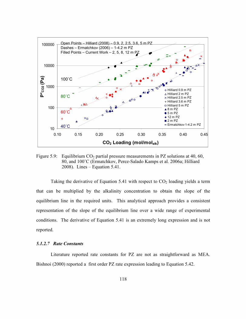
118

10

100

1000

10000

100000

0.10 0.15 0.20 0.25 0.30 0.35 0.40 0.45


P* C

O2 (Pa)

Hilliard 0.9 m PZ


Hilliard 3.6 m PZ


5 m PZ

12 m PZ2 m PZ





100˚C

80˚C

60˚C

40˚C10

100

1000

10000

100000

0.10 0.15 0.20 0.25 0.30 0.35 0.40 0.45


P* C

O2 (Pa)

Hilliard 0.9 m PZ


Hilliard 3.6 m PZ


5 m PZ

12 m PZ2 m PZ





100˚C

80˚C

60˚C

40˚C

Figure 5.9: Equilibrium CO2 partial pressure measurements in PZ solutions at 40, 60, 80, and 100˚C (Ermatchkov, Perez-Salado Kamps et al. 2006a; Hilliard 2008). Lines – Equation 5.41.

Taking the derivative of Equation 5.41 with respect to CO2 loading yields a term

that can be multiplied by the alkalinity concentration to obtain the slope of the

equilibrium line in the required units. This analytical approach provides a consistent

representation of the slope of the equilibrium line over a wide range of experimental

conditions. The derivative of Equation 5.41 is an extremely long expression and is not

reported.

5.1.2.7 Rate Constants

Literature reported rate constants for PZ are not as straightforward as MEA.

Bishnoi (2000) reported a first order PZ rate expression leading to Equation 5.42.

119

1137 600,33exp1014.4 −−

−⋅= smolmRT

kPZ (5.42)

Derks (2006) also reported a first order PZ rate expression. Derks suggests the

rate constant expression in Equation 5.43.

1137 100,34exp1057.6 −−

−⋅= smolmRT

kPZ (5.43)

Cullinane uses a rigorous kinetic model to interpret rate constants. Cullinane

reports a second order piperazine dependence but reports a separate rate constant for each

amine-base pairing. The rate expression used by Cullinane is similar to the expression

(Equation 5.40) used in this work and is shown below.

[ ][ ][ ]22COBAmkr

B

BAmCO ∑ −= (5.44)

The Cullinane model cannot be compared to the first order models by Derks

(2006) and Bishnoi (2000). It is also difficult to compare to the current model because

the current model is activity-based while the Cullinane model is concentration-based.

Cullinane reports an activation energy of 35 kJ/mol which is similar to the 33.6

and 34.1 kJ/mol reported by Bishnoi (2000) and Derks (2006). The current model also

utilizes an activation energy of 35 kJ/mol.

The rate expression (Equation 5.39 or 5.40) has 2 pre-exponential constants. The

value for kPZCOO was assumed to be 70% of kPZ. This 70% value was used by Cullinane

for the reported kPZ-PZ, kPZ-PZCOO, kPZCOO-PZ, and kPZCOO-PZCOO rate constants. The 70%

ratio is based on Bronsted theory which relates the pKa of a base to its rate constant.

With kPZCOO ratioed to kPZ, the kPZ pre-exponential rate constant was adjusted until the

expression in Equation 5.45 was minimized.

120

∑

−2

'

,

'

,

'

,

measg

measgcalcg

k

kk (5.45)

The values of kPZ and kPZCOO are 6.9·107 and 4.8·10

7 m

6mol

–2s–1, respectively, in

the final rate expression shown in Equation 5.46. This rate expression leads to the

following expression for kg’ in aqueous PZ.

[ ] [ ] [ ][ ] [ ][ ]

[ ]222

22

2 CO

PZCOOk

PZPZCOOk

PZCOOPZkPZk

r

PZCOOPZCOO

PZPZCOOPZCOO

PZCOOPZPZPZPZ

CO ⋅

+

+

+

−=−

−

−

γ

γγ

γγγ (5.46)

[ ] [ ] [ ][ ] [ ][ ]

[ ]

∆

∆+

+

+

+=

−

−

−T

o

CO

PZCOOPZCOO

PZPZCOOPZCOO

PZCOOPZPZPZPZ

OHCOCO

gCO

P

k

D

PZCOOk

PZPZCOOk

PZCOOPZkPZk

H

k

CO

prodl 2

*

2

22

22

2,2

5.0

2

'

2

,

11

γ

γγ

γγγ

γ (5.47)

5.2 SPREADSHEET MODEL ANALYSES

With the framework for the MEA and PZ spreadsheet models defined, each model

can now be analyzed. This section looks at how each parameter in the modified kg’

expression is affected by changes in temperature, amine concentration, and CO2 loading.

Wetted wall column experiments have shown that neither temperature nor amine

concentration changes significantly affect kg’ for MEA and often PZ systems (Figures 4.7

and 4.8). This section explains why kg’ is often independent of temperature and amine

concentration.

This section also compares model results to applicable literature data and

extrapolates the model to explore kg’ at 20˚C. The 20˚C case may be feasible in cold

locations such as the North Sea.

121

The final form of the kg’ expressions can be written as Equation 5.48 and 5.49 for

MEA and PZ, respectively. The first term in the kg’ expressions represents the pseudo

first order condition. The second term represents the mass transfer resistance due to

diffusion of reactants and products near the reaction interface.

[ ]

∆

∆+=

T

o

COMEA

OHCOCO

gCO

P

kDMEAk

H

k

CO

prodl 2

*

2

22

2,2

5.0

2

'

2

,

1

][

1

γ

γ (5.48)

[ ] [ ] [ ][ ] [ ][ ]

[ ]

∆

∆+

+

+

+=

−

−

−T

o

CO

PZCOOPZCOO

PZPZCOOPZCOO

PZCOOPZPZPZPZ

OHCOCO

gCO

P

k

D

PZCOOk

PZPZCOOk

PZCOOPZkPZk

H

k

CO

prodl 2

*

2

22

22

2,2

5.0

2

'

2

,

11

γ

γγ

γγγ

γ (5.49)

5.2.1 Monoethanolamine

5.2.1.1 Parameter Determination

This section shows how each of the parameters in Equation 5.48 changes with

temperature, amine concentration, and CO2 loading.

The rate constant is independent of amine concentration and CO2 loading. Figure

5.10 shows the temperature effect on the rate constant.

122

0.01

0.1

1

10

20 40 60 80 100 120

Temperature (C)

k (m

6. mol-2. s)

Figure 5.10: Calculated MEA rate constant from 20–120˚C

The MEA rate constant greatly increases with increasing temperature, two orders

of magnitude from 20–120˚C. The rate constant has a 0.5 order effect on the pseudo first

order term in Equation 5.48.

The MEA activity coefficient is also independent of amine concentration. Figure

5.11 shows how the MEA activity coefficient is affected by changes in temperature and

CO2 loading.

MEA

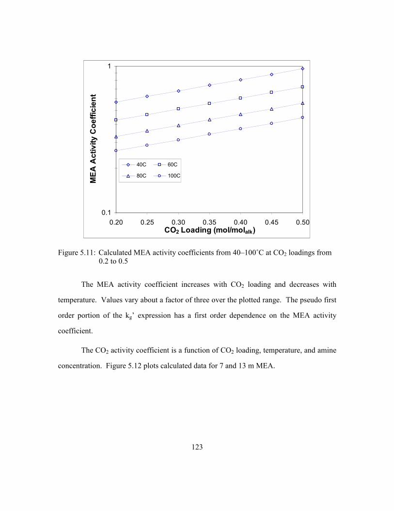
123

0.1

1

0.20 0.25 0.30 0.35 0.40 0.45 0.50CO2 Loading (mol/molalk)


40C 60C

80C 100C

Figure 5.11: Calculated MEA activity coefficients from 40–100˚C at CO2 loadings from 0.2 to 0.5

The MEA activity coefficient increases with CO2 loading and decreases with

temperature. Values vary about a factor of three over the plotted range. The pseudo first

order portion of the kg’ expression has a first order dependence on the MEA activity

coefficient.

The CO2 activity coefficient is a function of CO2 loading, temperature, and amine

concentration. Figure 5.12 plots calculated data for 7 and 13 m MEA.

124

_ _ _ 13 m MEA

_____ 7 m MEA

1

10

0.20 0.25 0.30 0.35 0.40 0.45 0.50


CO2 Activity Coefficient

40C

60C

80C

100C

Figure 5.12: Calculated CO2 activity coefficients from 40–100˚C at CO2 loadings from 0.2 to 0.5 in 7 and 13 m MEA

The activity coefficient of CO2 increases with MEA concentration and CO2

loading and decreases with increasing temperature. CO2 activity coefficient values vary

about a factor of two over the plotted range. The CO2 activity coefficient has a –0.5

order effect on the pseudo first order kg’ expression.

The free MEA concentration is a strong function of CO2 loading and amine

concentration. It is also a slight function of temperature due to changes in speciation.

Figure 5.13 plots the data for 7 and 13 m MEA.

125

_ _ _ 13 m MEA

_____ 7 m MEA

0.1

1

10

0.20 0.25 0.30 0.35 0.40 0.45 0.50


[MEA] F

ree (mol/L)

40C

60C

80C

100C

Figure 5.13: Free MEA concentration from 40–100˚C for 7 and 13 m MEA (Hilliard 2008)

Figure 5.13 shows a minor effect of temperature on free MEA. The free amine

concentration decreases with both increasing CO2 loading and decreasing total MEA

concentration. The change with CO2 loading is particularly important since the free

MEA concentration can change more than one order of magnitude over the lean to rich

CO2 loading range. The free MEA concentration has a first order effect on the pseudo

first order portion of the kg’ expression in Equation 5.48.

The diffusion coefficient of CO2 is affected by CO2 loading, temperature, and

amine concentration since each of these parameters affects viscosity. Figure 5.14 shows

how the calculation of the diffusion coefficient of CO2 is affected by changes in each of

the three parameters.

126

_ _ _ 13 m MEA

_____ 7 m MEA

1.E-10

1.E-09

1.E-08

0.20 0.25 0.30 0.35 0.40 0.45 0.50


DCO2 (m

2/s)

40C 60C 80C 100C

Figure 5.14: Calculated diffusion coefficient of CO2 for 40–100˚C at 0.2–0.5 CO2 loadings in 7 and 13 m MEA

CO2 loading has a minor effect on the diffusion coefficient of CO2. Both amine

concentration and temperature strongly affect the DCO2. The data shown in Figure 5.14

exhibit a full order of magnitude difference between the lowest and highest DCO2 values.

The pseudo first order portion of the kg’ expression has a 0.5 order dependence on the

diffusion coefficient of CO2

5.2.1.2 Parameter Significance

The previous section has shown how each of the parameters in Equation 5.48

varies with changes in CO2 loading, temperature, and MEA concentration. However,

many of the parameters have different orders in the kg’ expression. This section attempts

to compare the significance of each parameter by showing changes in each parameter at

127

common conditions. The correct order is implemented for each parameter. The order of

the parameters is only significant to the pseudo first order portion of Equation 5.48. If

diffusion becomes a significant resistance at a given condition, the pseudo first order part

of Equation 5.48 becomes less meaningful.

Figures 5.15–5.17 are plotted against CO2 loading for some extreme conditions: 7

and 13 m MEA. For each parameter the correct order in Equation 5.48 is incorporated.

Since Figures 5.15–5.17 each have stated temperatures, only the free MEA concentration,

diffusion coefficient of CO2, and the activity coefficients vary. The values of the rate

constant and the Henry’s solubility in water would remain constant in each graph.

7 m MEA 40C

0.1

1

10

0.2 0.25 0.3 0.35 0.4 0.45 0.5


Parameters

(SI units)

1E-07

1E-06

1E-05

kg' (mol/s. Pa. m

2)

Gamma MEA [MEA] x 10 -3DCO2 0.5 x 10 4 1/(Gamma CO2) 0.5PFO kg' Calc kg'

Figure 5.15: Parameter significance against CO2 loading for 7 m MEA at 40˚C

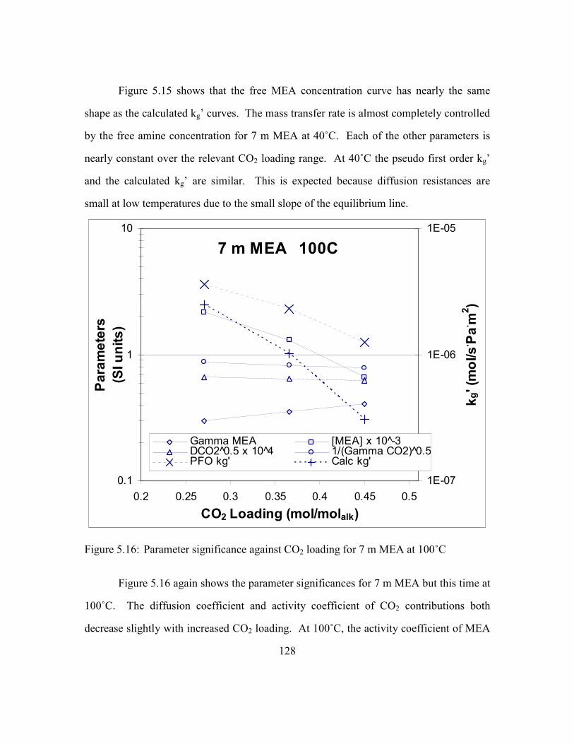
128

Figure 5.15 shows that the free MEA concentration curve has nearly the same

shape as the calculated kg’ curves. The mass transfer rate is almost completely controlled

by the free amine concentration for 7 m MEA at 40˚C. Each of the other parameters is

nearly constant over the relevant CO2 loading range. At 40˚C the pseudo first order kg’

and the calculated kg’ are similar. This is expected because diffusion resistances are

small at low temperatures due to the small slope of the equilibrium line.

7 m MEA 100C

0.1

1

10

0.2 0.25 0.3 0.35 0.4 0.45 0.5


Parameters

(SI units)

1E-07

1E-06

1E-05

kg' (mol/s. Pa. m

2)

Gamma MEA [MEA] x 10 -3DCO2 0.5 x 10 4 1/(Gamma CO2) 0.5PFO kg' Calc kg'


Figure 5.16 again shows the parameter significances for 7 m MEA but this time at

100˚C. The diffusion coefficient and activity coefficient of CO2 contributions both

decrease slightly with increased CO2 loading. At 100˚C, the activity coefficient of MEA

129

has a stronger effect than at 40˚C. Changes in kg’ result primarily from the change in free

MEA. The pseudo first order kg’ and the calculated kg’ vary significantly at low loading

and even more at higher loading. At 100˚C, MEA solutions encounter significant

diffusion resistances that limit CO2 mass transfer.

13 m MEA 60C

0.1

1

10

0.2 0.25 0.3 0.35 0.4 0.45 0.5


Parameters

(SI units)

1E-07

1E-06

1E-05

kg' (mol/s. Pa. m

2)

Gamma MEA [MEA] x 10 -3DCO2^0.5 x 10^4 1/(Gamma CO2) 0.5PFO kg' Calc kg'


In 13 m MEA at 60˚C, both the activity and diffusion coefficients of CO2 show a

decrease, essentially canceling the increase of the MEA activity coefficient. Again,

changes in the free amine concentration dominate changes in kg’. At 60˚C, there is a

small diffusion resistance in the system. This resistance causes the pseudo first order kg’

and the calculated kg’ to diverge slightly at the higher CO2 loading conditions.

130

Figure 5.18 looks directly at the effect of the parameters as a function of

temperature. An intermediate condition of 9 m MEA at 0.3 CO2 loading was selected for

this analysis.

9 m MEA 0.3 CO2 Loading

0.1

1

10

40 50 60 70 80 90 100

Temperature (C)

Parameters

(SI units)

1E-06

1E-05

kg' (mol/s. Pa. m

2)

Gamma MEA [MEA] x 10 -3DCO2^0.5 x 10^4 1/(Gamma CO2)^0.5k^0.5 1/HCO2,H2O*10 -4PFO kg' Calc kg'

Figure 5.18: Parameter significance against temperature for 9 m MEA at 0.3 CO2 loading

In agreement with the experimental data, Figure 5.18 shows that kg’ is mostly

independent of temperature in MEA solutions. However, the parameters which comprise

the kg’ expression have strong temperature dependences. The Henry’s solubility in water,

the rate constant, the activity coefficient of MEA and the diffusion coefficient of CO2 are

all strongly affected by temperature. However, all these increasing and decreasing effects

mostly cancel each other. The pseudo first order kg’ shows about a 50% increase over the

131

temperature range but that increase is negated by the increased diffusion resistance at

higher temperature. The calculated kg’ is relatively but does have a maximum at

intermediate temperatures. A critical look at Figure 4.7 shows that this phenomenon was

seen for MEA experiments in the wetted wall column.

Figure 5.19 shows the significance of each parameter with changes in amine

concentration. 60˚C solutions with a 0.4 CO2 loading were selected for this analysis.

60C 0.4 CO2 Loading

0.1

1

10

7 8 9 10 11 12 13

MEA Concentration (molality)

Parameters

(SI units)

1E-06

1E-05

kg' (mol/s. Pa. m

2)

Gamma MEA [MEA] x 10 -3DCO2^0.5 x 10^4 1/(Gamma CO2)^0.5k^0.5 1/HCO2,H2O*10^-4PFO kg' Calc kg'

Figure 5.19: Parameter significance against MEA concentration for 60˚C and 0.4 CO2 loading

Figure 5.19 explains exactly why wetted wall column experiments have shown

that kg’ is independent of MEA concentration. With changes in MEA concentration,

132

most of the parameters are relatively constant in their effect on kg’. Only the diffusion

coefficient of CO2, the activity coefficient of CO2, and the free amine concentration vary

significantly and those dependences essentially cancel each other. Figure 5.19 also

shows an equal spacing between the pseudo first order and calculated kg’ values over the

entire MEA concentration range. This suggests that the ratio of the kinetic and diffusion

resistances does not change with MEA concentration.

Figure 5.20 shows the importance of the diffusion resistance in 7 and 13 m MEA

over the range of experimental temperatures.

_ _ _ 13 m MEA

_____ 7 m MEA

0

0.2

0.4

0.6

0.8

0.20 0.25 0.30 0.35 0.40 0.45 0.50


Fraction of Mass Transfer

Resistance from Diffusion

40C 60C

80C 100C

Figure 5.20: Fraction of mass transfer resistance from diffusion for 40–100˚C, 7 and 13 m MEA

Figure 5.20 shows more clearly that the amine concentration does not affect the

ratio of the resistances due to kinetics and diffusion in Equation 5.48. Figure 5.19 shows

that the pseudo first order kg’ does not change significantly with MEA concentration.

133

This implies that the value of the diffusion resistance does not change very much either

with amine concentration. At higher MEA concentration, the physical liquid film mass

transfer coefficient, klo, decreases due to viscosity changes. However, the slope of the

equilibrium line also has a concentration term since it must be defined in Pa/(mol/m3).

The increased concentration decreases the slope of the equilibrium line. The diffusion

term in Equation 5.48 divides klo by the slope and that term is mostly unchanged with

changes in total MEA concentration.

At high temperature, particularly 100˚C, diffusion limits mass transfer even at

moderate CO2 loadings. This is mainly due to a drastic increase in the slope of the

equilibrium line in Equation 5.48.

5.2.1.3 Error Analysis

This analysis seeks to show that systematic error has been removed from the

model with respect to changing temperature, CO2 loading, and MEA concentration. The

lack of systematic error provides a better confidence in the estimation of the parameters

which comprise the kg’ expression, Equation 5.48.

Figure 5.21 shows an overall graph of all the wetted wall column data: 7–13 m

MEA, 40–100˚C, 0.23–0.50 CO2 loading. A parity plot is used to compare measured

wetted wall column kg’ values to the calculated kg’ from Equation 5.48.

134

1E-07

1E-06

1E-05

1E-07 1E-06 1E-05

Measured kg' (mol/s .Pa.m 2)

Calculated k

g' (m

ol/s. Pa. m

2)

7 m 40C 7 m 60C9 m 40C 9 m 60C11 m 40C 11 m 60C13 m 40C 13 m 60C7 m 80C 7 m 100C9 m 80C 9 m 100C11 m 80C 11 m 100C13 m 80C 13 m 100C

Figure 5.21: Parity plot comparing experimentally measured MEA kg’ values to kg’ values calculated from Equation 5.48

Figure 5.21 shows that kg’ values vary about a factor of 30 from the lowest

loading to the highest loading conditions. A brief view shows that all of the points fall

relatively close to the parity line. Equation 5.48 represents the measured wetted wall

column kg’ in aqueous MEA with an average error of 13%.

Figure 5.22 includes all the data in Figure 5.21 but is plotted differently to show

systematic trends with CO2 loading.

135

7-13 m MEA

40-100C0.5

1

1.5

0.2 0.25 0.3 0.35 0.4 0.45 0.5


kg' calc/kg' m

eas

Figure 5.22: Calculated/measured kg’ against CO2 loading for all MEA wetted wall column conditions

Figure 5.22 has dotted lines to show ±15 and 40% error in the estimation of kg’.

All of the data fall within 40% of the measured kg’ values. This is impressive, since kg’

values vary about a factor of 30. Many of the parameters comprising the kg’ expression

change considerably with changes in temperature, MEA concentration, and CO2 loading.

Overall, there does not seem to be a systematic trend with changes in CO2 loading since

the points are centered around the y=1 line.

Figure 5.23 plots all the experimental data against temperature.

+40%

-40%

-15%

+15%

136

7-13 m MEA

0.23-0.50 CO2 Loading

0.5

1

1.5

30 40 50 60 70 80 90 100 110

Temperature (C)

kg' calc/kg' m

eas

Figure 5.23: Calculated/measured kg’ against temperature for all MEA wetted wall column conditions

Figure 5.23 shows a systematic error with increasing temperature. According to

Figure 5.18, many of the parameters comprising kg’ vary considerably with changes in

temperature. The slope of the equilibrium line is also extremely sensitive to temperature.

Considering how sensitive Equation 5.48 is to changes in temperature, the systematic

error shown in Figure 5.23 is relatively small. The systematic temperature error is about

4 kJ/mol. This can be compared to the MEA activation energy of 45 kJ/mol (Equation

5.27). However, the activation energy should not be adjusted to remove the error since

the activation energy is known with more certainty than the other temperature dependent

terms in the kg’ expression. This systematic error with temperature has not been removed

from the model.

+40%

-40%

-15%

+15%

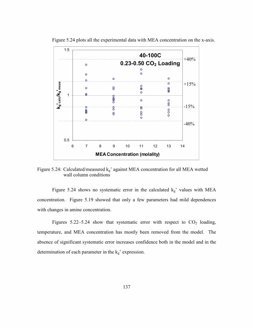
137

Figure 5.24 plots all the experimental data with MEA concentration on the x-axis.

40-100C


0.5

1

1.5

6 7 8 9 10 11 12 13 14

MEA Concentration (molality)

kg' calc/kg' m

eas

Figure 5.24: Calculated/measured kg’ against MEA concentration for all MEA wetted wall column conditions

Figure 5.24 shows no systematic error in the calculated kg’ values with MEA

concentration. Figure 5.19 showed that only a few parameters had mild dependences

with changes in amine concentration.

Figures 5.22–5.24 show that systematic error with respect to CO2 loading,

temperature, and MEA concentration has mostly been removed from the model. The

absence of significant systematic error increases confidence both in the model and in the

determination of each parameter in the kg’ expression.

+40%

+15%

-40%

-15%

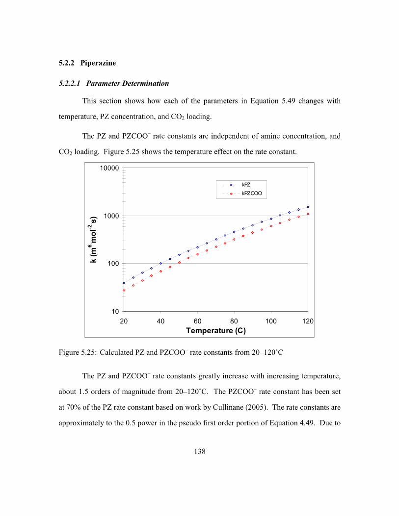
138

5.2.2 Piperazine

5.2.2.1 Parameter Determination

This section shows how each of the parameters in Equation 5.49 changes with

temperature, PZ concentration, and CO2 loading.

The PZ and PZCOO– rate constants are independent of amine concentration, and

CO2 loading. Figure 5.25 shows the temperature effect on the rate constant.

10

100

1000

10000

20 40 60 80 100 120

Temperature (C)

k (m

6. mol-2. s)

kPZ

kPZCOO

Figure 5.25: Calculated PZ and PZCOO– rate constants from 20–120˚C

The PZ and PZCOO– rate constants greatly increase with increasing temperature,

about 1.5 orders of magnitude from 20–120˚C. The PZCOO– rate constant has been set

at 70% of the PZ rate constant based on work by Cullinane (2005). The rate constants are

approximately to the 0.5 power in the pseudo first order portion of Equation 4.49. Due to

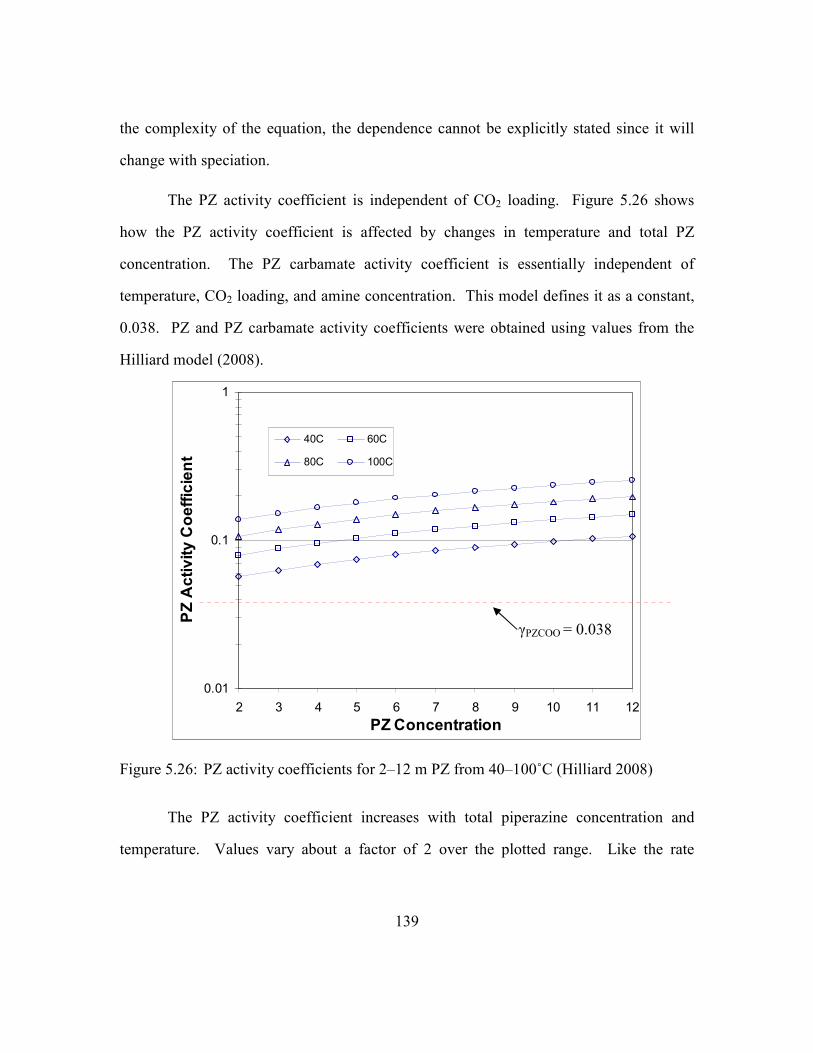
139

the complexity of the equation, the dependence cannot be explicitly stated since it will

change with speciation.

The PZ activity coefficient is independent of CO2 loading. Figure 5.26 shows

how the PZ activity coefficient is affected by changes in temperature and total PZ

concentration. The PZ carbamate activity coefficient is essentially independent of

temperature, CO2 loading, and amine concentration. This model defines it as a constant,

0.038. PZ and PZ carbamate activity coefficients were obtained using values from the

Hilliard model (2008).

0.01

0.1

1

2 3 4 5 6 7 8 9 10 11 12

PZ Concentration

PZ Activity Coefficient

40C 60C

80C 100C

Figure 5.26: PZ activity coefficients for 2–12 m PZ from 40–100˚C (Hilliard 2008)

The PZ activity coefficient increases with total piperazine concentration and

temperature. Values vary about a factor of 2 over the plotted range. Like the rate

γPZCOO = 0.038

140

constants, Equation 5.49 does not define an explicit order for the PZ activity coefficient,

but is approximately first order in the pseudo first order expression.

The CO2 activity coefficient is a function of CO2 loading, temperature, and amine

concentration. Figure 5.27 plots the calculations for 2 and 12 m PZ.

_ _ _ 12 m PZ

_____ 2 m PZ

1

10

0.20 0.25 0.30 0.35 0.40 0.45


CO2 Activity Coefficient

40C

60C

80C

100C

Figure 5.27: Calculated CO2 activity coefficients at 40–100˚C with 0.2 to 0.45 CO2 loadings in 2 and 12 m PZ

The activity coefficient of CO2 increases with PZ concentration and CO2 loading

and decreases with increasing temperature. CO2 activity coefficient values vary about a

factor of 10 over the plotted range. The CO2 activity coefficient has a –0.5 order effect

on the pseudo first order portion of the kg’ expression.

The free PZ and PZCOO– concentrations are a function of CO2 loading and amine

concentration. They are also a function of temperature since the solution speciation

141

changes with temperature. Figure 5.28 plots the free PZ concentrations for 2 and 8 m PZ.

Figure 5.29 plots the free PZCOO– concentrations for 2 and 8 m PZ. These values were

obtained from the Hilliard model (2008).

_ _ _ 8 m PZ

_____ 2 m PZ

0.01

0.1

1

10

0.20 0.25 0.30 0.35 0.40 0.45


[PZ] Free (mol/L)

40C

60C

80C

100C

Figure 5.28: Free PZ concentration from 40–100˚C for 2 and 8 m PZ (Hilliard 2008)

Oddly, free piperazine concentrations for 2 m and 8 m PZ are almost equivalent at

constant CO2 loading. This suggests that the total amine concentration plays a large part

in the speciation of PZ solutions. Overall, the free PZ concentration varies about a factor

of 10 from lean to rich conditions.

142

_ _ _ 8 m PZ

_____ 2 m PZ

0.01

0.1

1

10

0.20 0.25 0.30 0.35 0.40 0.45


[PZCOO- ] (mol/L)

40C

60C

80C

100C

Figure 5.29: PZCOO– concentration from 40–100˚C for 2 and 8 m PZ (Hilliard 2008)

Figure 5.29 shows a large difference in the PZCOO– concentrations for 2 and 8 m

PZ. This was expected since free PZ concentrations are fairly similar in the Hilliard

model. The piperazine material balance must be satisfied. The free PZ concentration is

also a significant function of temperature, especially for the 2 m solution. Again, the

order of the free PZ and PZCOO– concentrations in Equation 5.49 is not explicit. They

are approximately first order since concentrations are squared under the square root.

Figure 5.30 shows the total free amine concentrations in 2 and 8 m PZ.

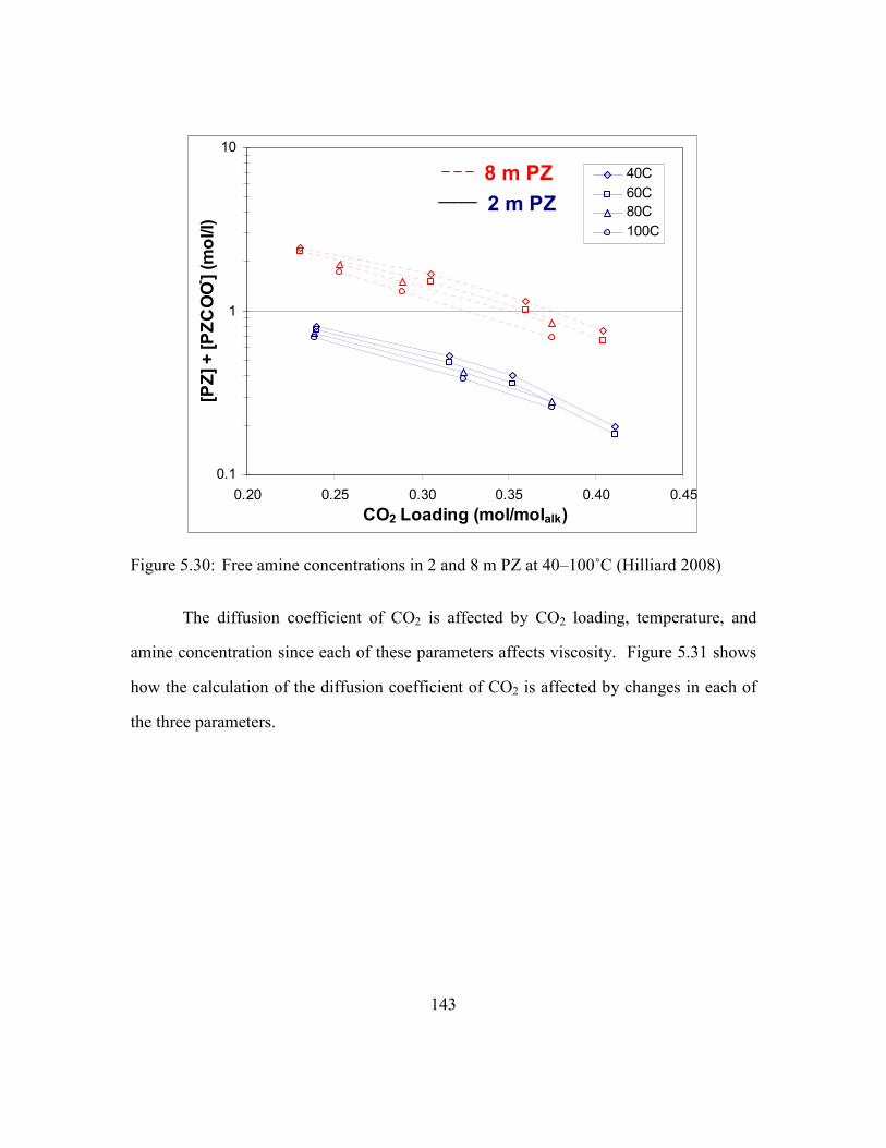
143

_ _ _ 8 m PZ

_____ 2 m PZ

0.1

1

10

0.20 0.25 0.30 0.35 0.40 0.45


[PZ] + [PZCOO- ] (mol/l)

40C

60C

80C

100C

Figure 5.30: Free amine concentrations in 2 and 8 m PZ at 40–100˚C (Hilliard 2008)

The diffusion coefficient of CO2 is affected by CO2 loading, temperature, and

amine concentration since each of these parameters affects viscosity. Figure 5.31 shows

how the calculation of the diffusion coefficient of CO2 is affected by changes in each of

the three parameters.

144

_ _ _ 8 m PZ

_____ 2 m PZ

1.E-10

1.E-09

1.E-08

0.20 0.25 0.30 0.35 0.40 0.45


DCO2 (m

2/s)

40C 60C

80C 100C

Figure 5.31: Calculated diffusion coefficient of CO2 from 40–100˚C in 2 and 8 m PZ

CO2 loading has a fairly minor effect on the diffusion coefficient of CO2. Both

amine concentration and temperature have strong effects on DCO2. Higher amine

concentrations and lower temperatures increase viscosity and thus lower diffusion

coefficients. The data shown in Figure 5.31 exhibit more than a full order of magnitude

difference between the lowest and highest DCO2 values. The diffusion coefficient of CO2

has a 0.5 order effect on the pseudo first order portion of the kg’ expression, Equation

5.49.

5.2.2.2 Parameter Significance

The previous section has shown how each of the parameters in Equation 5.49 vary

with changes in CO2 loading, temperature, and MEA concentration. However, many of

the parameters have different powers in the kg’ expression. Some of these powers must

145

be approximated due to the form of Equation 5.49. This section attempts to compare the

significance of each parameter by showing the changes in each parameter at common

conditions. Note that the order of the parameters is only significant to the pseudo first

order portion of Equation 5.49. If diffusion becomes significant at a given condition, the

pseudo first order part of Equation 5.49 becomes less meaningful.

Figures 5.32–5.34 are plotted against CO2 loading for some extreme conditions: 2

and 12 m PZ. For each parameter the explicit or approximated power in Equation 5.49 is

incorporated. Since Figures 5.32–5.34 each have stated temperatures, only the free PZ

and PZCOO– concentrations, diffusion coefficient of CO2, and the activity coefficient of

CO2 vary. The rate constant and the Henry’s solubility in water are constant in each

graph.

146

2 m PZ 40C

0.01

0.1

1

0.20 0.25 0.30 0.35 0.40 0.45


Parameters

(SI units)

1E-07

1E-06

1E-05

kg' (mol/s. Pa. m

2)

[PZ] x 10 -3 DCO2 0.5 x 10 41/(Gamma CO2) 0.5 [PZCOO] x 10 -3PFO kg' Calc kg'

Figure 5.32: Parameter significance against CO2 loading for 2 m PZ at 40˚C

Figure 5.32 shows that for 2 m PZ at 40˚C, the effects of the activity and diffusion

coefficients of CO2 are minor with CO2 loading changes. The change in the liquid film

mass transfer coefficient, kg’, with increased CO2 loading is almost completely controlled

by the free amine concentrations. The calculated and pseudo first order kg’ calculations

are almost identical at this 40˚C condition. This implies that diffusion resistances are

negligible. At 40˚C, the slope of the equilibrium line is very small, making the second

term in Equation 5.49 of minor significance.

147

2 m PZ 100C

0.01

0.1

1

0.20 0.25 0.30 0.35 0.40 0.45


Parameters

(SI units)

1E-07

1E-06

1E-05

1E-04

kg' (mol/s. Pa. m

2)

[PZ] x 10 -3DCO2 0.5 x 10 41/(Gamma CO2) 0.5[PZCOO] x 10 -3PFO kg'Calc kg'


Figure 5.33 shows the significance of parameters in 2 m PZ at 100˚C. The

diffusion and activity coefficients of CO2 change insignificantly with CO2 loading. At

low loading, PZCOO– concentration again remains relatively unchanged. The change in

the pseudo first order slope is almost completely due to the change in the free PZ

concentration. The parameters range two decades in Figure 5.33 while the kg’ scale

includes three decades. Since this 100˚C condition is significantly affected by diffusion

resistances, the calculated kg’ values fall far below pseudo first order kg’ values. The

drop is even greater at the higher loading since less free amine is available. The diffusion

of fresh amine to the interface severely limits mass transfer in this case.

148

12 m PZ 60C

0.01

0.1

1

10

0.20 0.25 0.30 0.35 0.40 0.45


Parameters

(SI units)

1E-07

1E-06

1E-05

kg' (mol/s. Pa. m

2)

[PZ] x 10 -3 DCO2^0.5 x 10^41/(Gamma CO2)^0.5 [PZCOO] x 10 -3PFO kg' Calc kg'


Figure 5.34 shows the parameter significance as a function of CO2 loading at

12 m PZ, 60˚C. This condition is not soluble at 0.4 loading so calculations have not been

made at that condition. Very similar to the previous two graphs, kg’ is almost completely

controlled by the change in the free PZ concentration. The free PZ carbamate

concentration begins to contribute to the drop in kg’ near 0.35 loading. Since this

solution is at 60˚C, there is a minor diffusion resistance which increases slightly with

increasing CO2 loading.

149

Figure 5.35 looks at the effect on the parameters as a function of temperature.

Intermediate conditions of 5 m PZ at 0.3 CO2 loading were selected for this analysis.

5 m PZ 0.3 CO2 Loading

0.1

1

10

40 50 60 70 80 90 100

Temperature (C)

Parameters

(SI units)

1E-06

1E-05

1E-04

kg' (mol/s. Pa. m

2)

Gamma PZ x 10 [PZ] x 10^-3DCO2^0.5 x 10^4 1/(Gamma CO2)^0.5kPZ^0.5*10^-1 1/HCO2,H2O*10 -4kPZCOO^0.5*10^-1 [PZCOO] x 10^-3PFO kg' Calc kg'

Figure 5.35: Parameter significance against temperature for 5 m PZ at 0.3 CO2 loading

Figure 5.35 shows that nearly all the parameters in Equation 5.49 are strongly

affected by temperature. Only the activity coefficient of CO2 dependence remains mostly

constant with changes in temperature. The contributions of the piperazine activity

coefficient, both rate constants, the free piperazine concentration, and the diffusion

coefficient of CO2 each increase significantly with increasing temperature. The

thermodynamic Henry’s constant (HCO2,H2O) and the PZCOO– concentration dependences

each decrease significantly with increasing temperature. Those 8 parameters provide a

150

significant increase in the pseudo first order rate expression with increasing temperature.

However, the higher temperature increases the diffusion resistance. The increased

diffusion resistance causes kg’ to remain relatively constant from 40 to 70˚C before it

begins to decrease. Overall, the predicted kg’ varies a factor of 2–3 despite seven

parameter dependences which vary factors of 2–3. The fact that the PZ model accurately

predicts the correct temperature behavior is remarkable considering the wide variance in

the parameters.

Figure 5.36 shows the significance of each parameter with changes in total

piperazine concentration. Only five parameters are included in Figure 5.36 since the

Henry’s constant, and rate constants do not change with temperature.

151

60C 0.4 CO2 Loading0.1

1

10

2 3 4 5 6 7 8 9 10 11 12

PZ Concentration

Parameters

(SI units)

1E-07

1E-06

1E-05

kg' (mol/s. Pa. m

2)

Gamma PZ x 10 [PZ] x 10 -2

DCO2^0.5 x 10^4 1/(Gamma CO2)^0.5

[PZCOO] x 10^-3 PFO kg'

Calc kg'

Figure 5.36: Parameter significance against PZ concentration for 60˚C and 0.4 CO2 loading

Overall, the parameters do not depend on piperazine concentration as much as

they depend on temperature. kg’ and kg’’ vary less than a factor of two over the 2–12 m

PZ range. An interesting point in Figure 5.36 is that the pseudo first order kg’ and the

non-pseudo first order kg’ remain evenly spaced. This implies that PZ concentration does

not affect the fraction of the diffusion resistance. Essentially, the ratio of the two terms in

Equation 5.49 is unaffected by PZ concentration.

Figure 5.37 explicitly shows the fraction of diffusion resistance for 2 and 8 m PZ.

152

_ _ _ 8 m PZ

_____ 2 m PZ

0

0.2

0.4

0.6

0.8

1

0.20 0.25 0.30 0.35 0.40 0.45


Fraction of Mass Transfer

Resistance from Diffusion

40C 60C

80C 100C

Figure 5.37: Fraction of mass transfer resistance from diffusion for 40–100˚C in 2 and 8 m PZ

As previously stated, the total PZ concentration does not affect the relative

importance of the two terms in Equation 5.49. The fraction of resistance due to diffusion

remains independent of PZ concentration. At higher concentrations, the physical liquid

film mass transfer coefficient, klo, decreases due to viscosity changes. However, the

slope of the equilibrium line has a concentration term since it is defined in Pa/(mol/m3).

The increased concentration decreases the slope of the equilibrium line. The diffusion

term in Equation 5.49 divides klo by the slope and that term is mostly unchanged with

changes in total PZ concentration.

153

5.2.2.3 Error Analysis

Like the MEA error analysis, this is not a typical error analysis. This analysis

seeks to show that most of the systematic error has been removed from the model. The

lack of systematic error provides a better confidence in the estimation of the parameters

which comprise the kg’ expression, Equation 5.49.

Figure 5.38 shows an overall graph of all the wetted wall column data: 2–12 m

PZ, 40–100˚C, 0.22–0.41 CO2 loading. A parity plot is used to compare measured wetted

wall column kg’ values to the calculated kg’ from Equation 5.49.

1E-07

1E-06

1E-05

1E-07 1E-06 1E-05

Measured kg' (mol/s .Pa.m 2)

Calculated k

g' (m

ol/s. Pa. m

2)

2 m 40C 2 m 60C5 m 40C 5 m 60C8 m 40C 8 m 60C12 m 60C 2 m 80C2 m 100C 5 m 80C5 m 100C 8 m 80C8 m 100C 12 m 80C12 m 100C

Figure 5.38: Parity plot comparing experimentally measured PZ kg’ values to kg’ values calculated from Equation 5.49.

154

Figure 5.38 shows that kg’ values vary about a factor of 20 from the lowest

loading to the highest loading conditions. A brief view shows that all of the points fall

relatively close to the parity line. There are no obvious trends with temperature or amine

concentration. However, to analyze and detect the systematic error, a closer look into the

data is required. Equation 5.49 represents the measured kg’ in PZ solutions with an

average error of 19%.

Figure 5.39 includes all the data in Figure 5.38 but is plotted differently to show

systematic trends in CO2 loading.

2-12 m PZ

40-100C

0.4

1

1.6

0.2 0.25 0.3 0.35 0.4 0.45


kg' calc/kg' m

eas

Figure 5.39: Calculated/measured kg’ against CO2 loading for 2–12 m PZ wetted wall column conditions

Figure 5.39 has dotted lines to show ±20 and 50% error in the estimation of kg’.

All but one of the data points fall within 50% of the measured kg’ values. This is

impressive considering the range of conditions. kg’ values vary about a factor of 20.

+50%

+20%

-20%

-50%

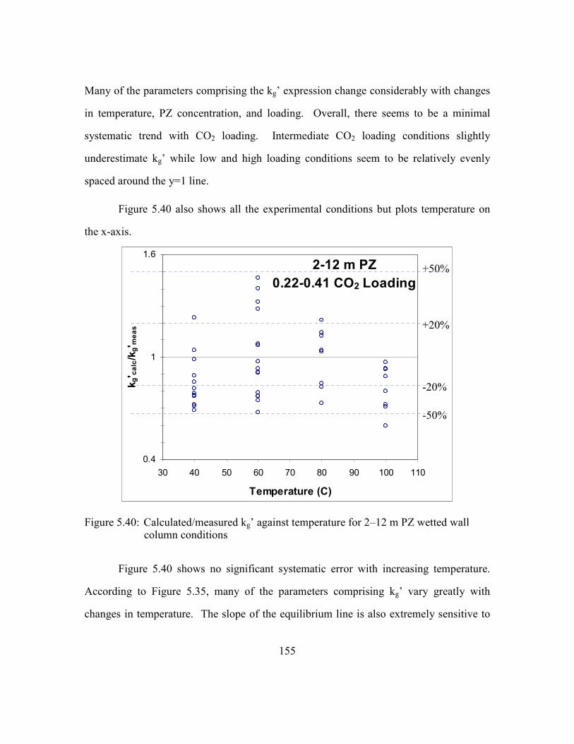
155

Many of the parameters comprising the kg’ expression change considerably with changes

in temperature, PZ concentration, and loading. Overall, there seems to be a minimal

systematic trend with CO2 loading. Intermediate CO2 loading conditions slightly

underestimate kg’ while low and high loading conditions seem to be relatively evenly

spaced around the y=1 line.

Figure 5.40 also shows all the experimental conditions but plots temperature on

the x-axis.

2-12 m PZ


0.4

1

1.6

30 40 50 60 70 80 90 100 110

Temperature (C)

kg' calc/kg' m

eas

Figure 5.40: Calculated/measured kg’ against temperature for 2–12 m PZ wetted wall column conditions

Figure 5.40 shows no significant systematic error with increasing temperature.

According to Figure 5.35, many of the parameters comprising kg’ vary greatly with

changes in temperature. The slope of the equilibrium line is also extremely sensitive to

-50%

+50%

-20%

+20%

156

temperature. The lack of systematic temperature error suggests that the temperature

dependent terms are being represented accurately.

Figure 5.41 plots all the experimental data with PZ concentration on the x-axis.

40-100C


0.4

1

1.6

0 2 4 6 8 10 12 14

PZ Concentration (molality)

kg' calc/kg' m

eas

Figure 5.41: Calculated/measured kg’ against PZ concentration for 2–12 m PZ wetted wall column conditions

Figure 5.41 shows no systematic error in the calculated kg’ values with PZ

concentration. Figure 5.43 showed that many of the parameters vary significantly with

changes in total PZ concentration. Regardless, the concentration dependent terms seem

to be properly represented.

Figures 5.39–5.41 show that systematic error with respect to CO2 loading,

temperature, and PZ concentration have essentially been removed from the model. The

absence of significant systematic error increases confidence both in the model and in the

-50%

-20%

+20%

+50%

157

determination of each parameter in the kg’ expression. The PZ model has fully explained

observed kg’ effects with changing temperature, CO2 loading, and piperazine

concentration.

5.2.3 Model Comparisons to Literature Data

5.2.3.1 MEA Model Comparisons to Literature Data

Figure 5.42 shows a comparison of the model to concentrated MEA rate data by

Aboudheir (2003) and Hartono (2009). Aboudheir uses a laminar jet absorber which has

a very fast liquid film physical mass transfer coefficient due to short contact times. To

compare to this pseudo first order condition, the pseudo first order results of the model

are plotted in Figure 5.42. The Hartono data can also be compared to the pseudo first

order model results since the diffusion of reactants and products is unimportant at

concentrated, unloaded conditions.

158

MEA

1E-07

1E-06

1E-05

0.0 0.1 0.2 0.3 0.4 0.5

CO2 Loading (molCO2/molalk)

kg' (mol/s. Pa. m

2)

Model 5 M, 40C, PFO Model 5 M, 60C, PFOModel 7 M, 40C, PFO Model 7 M, 60C, PFOAboudheir 5 M, 40C Aboudheir 5 M, 60CAboudheir 7 M, 40C Aboudheir 7 M, 60CHartono 5 M, 40C

Figure 5.42: Pseudo first order model results compared to 5 and 7 M MEA literature data (Aboudheir, Tontiwachwuthikul et al. 2003; Hartono 2009)

The pseudo first order model results for both 7 and 13 m show temperature trends

similar to the Aboudheir data. The model also matches the kg’ values fairly well over the

entire CO2 loading range. The model shows a more drastic change in kg’ at higher

loading. This was seen in all the experimental data (Figure 4.10). The wetted wall

column experimental data could not justify the flattening of the kg’ values at lower CO2

loading. The model predicts this observed trend.

The model can also be extrapolated to zero loading and more dilute MEA

concentrations to evaluate recent data by Hartono (2009).

159

Unloaded MEA at 40C

1E-07

1E-06

1E-05

0 1 2 3 4 5

MEA Concentration (Molarity)

kg' (mol/s. Pa. m

2)

Model 40C

Hartono

Figure 5.43: MEA model comparison to Hartono (2009) at 40˚C

Overall, the data seem to match the Hartono data adequately. Rates are

underpredicted at low MEA concentrations and slightly overpredicted at high MEA

concentrations. The model neglects base catalysis by water. This could be a significant

contribution to the rates at very low MEA concentrations.

5.2.3.2 Comparison to Cullinane (2006) Piperazine Rate Constants

Figure 4.12 has shown that 1.8 m PZ from the Cullinane model (2005) compares

very favorably to 2 m PZ experiments in the wetted wall column. This analysis also

seeks to compare the rate expressions.

Due to differences in the form of the Cullinane rate expression and the form of the

rate expression used in this work (Equation 5.40), it is difficult to make a straightforward

rate constant comparison. An attempt has been made to compare unloaded 1 M PZ.

160

Cullinane (2006) reports an overall rate constant of 102,000 s–1 at 25˚C for

unloaded 1 M PZ. This value results from the combination of the o

PZPZk − and o

OHPZk2−

rate constants multiplied by the piperazine and water molarity, respectively. This model

ignores the water catalysis effect. At 1 M PZ this effect can be significant. It is easier to

exclude the water catalysis from the Cullinane expression to obtain a 70,100 s–1 rate

expression only considering PZ catalysis.

The current model can be extrapolated to 1 M but the difference in the form of the

rate expressions must be considered. Cullinane utilized a concentration-based model.

The CO2 activity coefficient approaches 1 for unloaded, dilute solutions. The unloaded

25˚C PZ activity coefficient was estimated as 0.0393 by the model. This model predicts

the rate constant times the square of the PZ activity coefficient to yield 78,600 s–1 at

25˚C. This compares very favorably to the 70,100 s–1 value reported by Cullinane

(2006).

5.2.3.3 Piperazine Model Comparisons to Literature Data

Figure 5.44 compares the PZ model to work done by Cullinane. Two unloaded,

1.2 M PZ data points are compared. A 1.8 m PZ model developed by Cullinane is also

compared. Although Cullinane did not measure rates in CO2 loaded aqueous PZ, he was

able to build the model using unloaded PZ and loaded K2CO2/PZ rate data.

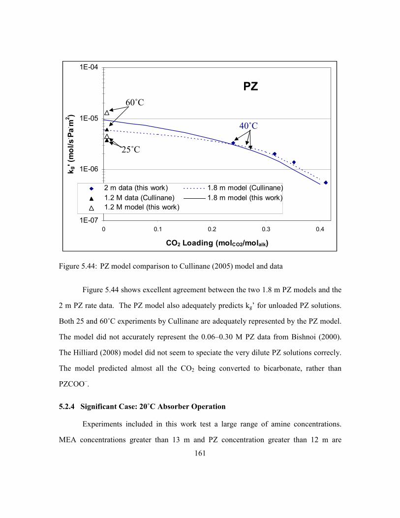
161

PZ

1E-07

1E-06

1E-05

1E-04

0 0.1 0.2 0.3 0.4


kg' (mol/s. Pa. m

2)

2 m data (this work) 1.8 m model (Cullinane)

1.2 M data (Cullinane) 1.8 m model (this work)

1.2 M model (this work)

Figure 5.44: PZ model comparison to Cullinane (2005) model and data

Figure 5.44 shows excellent agreement between the two 1.8 m PZ models and the

2 m PZ rate data. The PZ model also adequately predicts kg’ for unloaded PZ solutions.

Both 25 and 60˚C experiments by Cullinane are adequately represented by the PZ model.

The model did not accurately represent the 0.06–0.30 M PZ data from Bishnoi (2000).

The Hilliard (2008) model did not seem to speciate the very dilute PZ solutions correcly.

The model predicted almost all the CO2 being converted to bicarbonate, rather than

PZCOO–.

5.2.4 Significant Case: 20˚C Absorber Operation

Experiments included in this work test a large range of amine concentrations.

MEA concentrations greater than 13 m and PZ concentration greater than 12 m are

40˚C

25˚C

60˚C

162

unlikely to be relevant for industrial use. The 40–100˚C temperatures also exhibit a large

range of conditions. 120˚C is not a particularly interesting condition because mass

transfer in those solutions would be almost completely controlled by diffusion

resistances. Special equipment designs, such as using trays instead of packing, could be

used to increase the physical liquid film mass transfer coefficient, klo. This model is not

very useful in evaluating that condition because klo in this model is based on the wetted

wall column. Amine solutions at 20˚C could be analyzed accurately by this model since

diffusion resistance would be negligible.

In some locations such as the North Sea it may be feasible to cool amine solutions

down to 20˚C. The colder amine solution would allow for a richer solution at the bottom

of the absorber. This analysis uses the spreadsheet models to explore the kinetic

implications of operating an absorber at 20˚C. The analysis has been carried out with 3

solutions, 7 and 13 m MEA and 8 m PZ.

The bottom of an absorber with flue gas from coal combustion will be

approximately 12% CO2 near atmospheric pressure. This 12 kPa partial pressure must be

significantly more than the partial pressure of the amine solution for significant

absorption to occur. Due to the reduction of CO2 driving force and the slower rates at the

bottom of the absorber it is unlikely that the amine solution would have a CO2 loading

exhibiting more than a 6 kPa partial pressure. Therefore 20˚C amine solutions are

analyzed up to a CO2 loading which has a 6 kPa CO2 partial pressure.

None of the 20˚C conditions encounter significant diffusion limitations so no

adjustment in klo is required to adjust to an industrial design.

163

5.2.4.1 7 and 13 m MEA

Using the spreadsheet model, the CO2 partial pressure and liquid film mass

transfer coefficient has been calculated for 0.25–0.6 loading in 7 and 13 m MEA. The

results are included in Table 5.4.

Table 5.4: Calculated CO2 partial pressure and kg’ for 7 and 13 m MEA at 20˚C

MEA Temp CO2 Loading P*CO2 kg'

m C molCO2/molalk Pa mol/s.Pa

.m

2

0.25 1.2 2.5E-06

0.3 3.1 2.1E-06

0.35 8.8 1.7E-06

0.4 28 1.2E-06

0.45 95 6.3E-07

0.5 353 1.7E-07

0.55 1433 3.7E-08

0.6 6345 1.5E-08

0.25 1.2 2.5E-06

0.3 3.1 2.0E-06

0.35 8.8 1.5E-06

0.4 28 1.0E-06

0.45 95 5.3E-07

0.5 353 8.7E-08

0.55 1433 1.2E-08

0.6 6345 5.6E-09

13

7

20

The values in Table 5.4 at 20˚C are compared to 40–100˚C conditions in Figure

5.45. 7 m MEA conditions are denoted by solid lines while 13 m MEA is represented by

dashed lines.

164

1E-09

1E-08

1E-07

1E-06

1E-05

1 10 100 1000 10000 100000

P*CO2 (Pa)

kg' (mol/s. Pa. m

2)

Figure 5.45: Predicted CO2 absorption/desorption rates in 7 and 13 m MEA at 20–100˚C

Figure 5.45 shows that the 20˚C solutions actually perform similarly to the higher

temperature data until near a 100 Pa partial pressure, 0.45 CO2 loading. Above this

loading the free amine concentration is too small to produce significant rates. Rates at

the rich end of the absorber in the 2–5 kPa range are 10 times slower than rates at 40˚C.

The 20˚C case is interesting because the colder temperatures allow for the amine

solution to achieve higher CO2 loading at the bottom of the absorber. The higher CO2

loading leads to a lower energy consumption in the stripper. However, for MEA, CO2

loadings at 20˚C seem too rich to produce acceptable rates. Operating with a 20˚C rich

solution at the bottom of the absorber does not seem to be advantageous for MEA

solutions.

_____7 m MEA

-----13 m MEA

20˚C 40˚C 60˚C 80˚C 100˚C

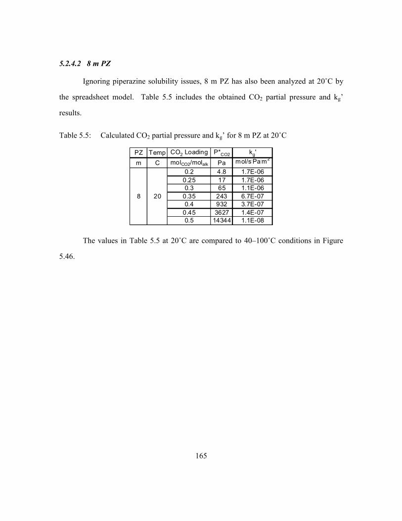
165

5.2.4.2 8 m PZ

Ignoring piperazine solubility issues, 8 m PZ has also been analyzed at 20˚C by

the spreadsheet model. Table 5.5 includes the obtained CO2 partial pressure and kg’

results.

Table 5.5: Calculated CO2 partial pressure and kg’ for 8 m PZ at 20˚C

PZ Temp CO2 Loading P*CO2 kg'

m C molCO2/molalk Pa mol/s.Pa

.m

2

0.2 4.8 1.7E-06

0.25 17 1.7E-06

0.3 65 1.1E-06

0.35 243 6.7E-07

0.4 932 3.7E-07

0.45 3627 1.4E-07

0.5 14344 1.1E-08

208

The values in Table 5.5 at 20˚C are compared to 40–100˚C conditions in Figure

5.46.

166

8 m PZ

1E-08

1E-07

1E-06

1E-05

1 10 100 1000 10000 100000

P*CO2 (Pa)

kg' (mol/s. Pa. m

2)

Figure 5.46: Predicted CO2 absorption/desorption rates in 8 m PZ at 20–100˚C

8 m PZ rates at the rich end of the absorber in the 2–5 kPa range are about 3 times

slower than rates at 40˚C. However, the 20˚C case achieves higher CO2 loadings and a

larger CO2 capacity which may yield enough energy savings to offset the slower rates. A

comprehensive absorber/stripper model incorporating both capital and operating costs

would be required to quantify if the 20˚C case is more economically favorable than the

40˚C condition. This analysis ignores PZ solubility issues.

5.2.5 MEA and Piperazine Rate Comparison

The MEA and PZ spreadsheet models accurately match experimental data.

Experimental measurements have shown PZ to react with CO2 2–3 times faster than

MEA. MEA and PZ reaction rates can also be compared through model results.

20˚C

40˚C 60˚C

80˚C

100˚C

167

Experiments show that kg’ is essentially independent of amine concentration and

temperature at lower temperatures. Figure 5.47 shows rate comparisons for 8 m PZ and 7

and 11 m MEA at 40˚C. Rates are compared at 40˚C because this is a likely temperature

at the rich end of the absorber column. Rich end kinetics are much more important than

lean end kinetics since rates are much slower at higher loading. Rich end kinetics

dominate absorber performance.

1E-07

1E-06

1E-05

10 100 1000 10000

P*CO2 @ 40C (Pa)

kg' (mol/s. Pa. m

2)

7 m MEA

11 m MEA

8 m PZ

Figure 5.47: 8 m PZ and 7 and 11 m MEA rate comparisons at 40˚C: points – data; lines – model

At rich end conditions (high loading or partial pressure) the model shows a larger

rate difference between MEA and PZ than the experimental data. If this trend is accurate,

the enhanced absorber performance with PZ will be greater than experimental results

suggest. Over the expected CO2 loading range, the model shows PZ rates 1.5–4 times

168

faster than MEA. At the rich end of the absorber, which dominates performance, PZ

absorbs CO2 about 3 times faster than MEA.

5.3 ASPEN PLUS® RATESEP™ MODELING

In addition to the spreadsheet models, an Aspen Plus® RateSep™ model was

created. Rather than predicting the mass transfer coefficient, kg’, the Aspen Plus®

RateSep™ model can predict CO2 flux. This model can be fitted to wetted wall column

data and then scaled up to industrial conditions.

As a starting point the electrolyte NRTL thermodynamic framework of the

Hilliard model (2008) was used. However, the Hilliard model is not capable of handling

the high amine concentration and high temperature conditions that were tested in the

wetted wall column experiments. Hilliard regressed data up to 11 m MEA and 5 m PZ.

CO2 partial pressure estimates are reliable up to 60˚C. Wetted wall column experiments

utilized amine concentrations up to 13 m MEA and 12 m PZ at 100˚C. The Hilliard

(2008) model did not accurately extrapolate to these higher amine concentrations.

5.3.1 Physical Design

The wetted wall column is modeled as an Aspen Plus® RateSep™ column. The

actual wetted wall column has an annulus geometry since the liquid film flows over a rod

and the gas flows around it. The Aspen Plus® RateSep™ module cannot mimic this

geometry. The column in the model was designed as a typical, cylindrical column. The

diameter was adjusted so the column would have the same cross-sectional area for gas

flow as the wetted wall column. This results in equivalent gas velocities in the wetted

wall column and the model. The design height of the column is the height of the wetted

wall column, 9.1 cm.

169

Mimicking the wetted area of the column requires a similar manipulation. In the

wetted wall column, the contact area is the surface area of a metal rod which is coated

with a thin film of liquid. The model assumes an arbitrary packing. An interfacial area

FORTRAN subroutine was written to ensure that the wetted area of the wetted wall

column, 38.52 cm2, would be duplicated in the model.

The model operates with 3 countercurrent stages. The model does not consider

pressure drop.

5.3.2 Primary Monoethanolamine Data Regression

A modified VLE model was created with the same sequential regression approach

that Hilliard employed. Hilliard (2008) used heat of absorption, nuclear magnetic

resonance, heat capacity, amine partial pressure and CO2 partial pressure data to regress

thermodynamic parameters. This model ignores the heat of absorption data.

The main MEA data regression includes nuclear magnetic resonance, heat

capacity, amine partial pressure, and CO2 partial pressure from Hilliard (2008).

Increased importance was placed on the MEA partial pressure data since these data lead

to MEA activity coefficients, which are very important to the rate behavior. CO2 partial

pressure data from Jou (1995) and Dugas (Rochelle, Sexton et al. 2009) were also

included in the regression. The MEA VLE model includes data ranging from 3.5 m

MEA to 13 m MEA with temperatures from 25 to 120˚C. Only data with CO2 loadings

between 0.25–0.6 molCO2/molMEA were included in the regression.

In an effort to simplify the regressions and obtain better CO2 partial pressure

predictions, significantly fewer parameters were regressed in this work than that of

Hilliard (2008). Some binary interaction parameter pairings were deemed insignificant

170

and deleted. The complexity of the temperature dependence of the molecule/anion-cation

pairings was simplified by deleting some of the temperature dependent terms.

Table 5.6 gives the regressed parameters for the system. Heat of formation, free

energy of formation, heat capacity, and molecule/anion-cation binary interaction

parameters were regressed. Figures 5.48–5.51 show the CO2 partial pressure fit of the

model against 7, 9, 11, and 13 m MEA. In each figure, the points include various amine

concentrations since amine concentration does not affect the CO2 partial pressure at CO2

loadings below 0.45.

Table 5.6: Regressed thermodynamic parameters for the MEA/CO2/H2O system

Parameter Component i Component j Value (SI units) Std Dev

DGAQFM/1 MEACOO- -4.96E+08 1.74E+11

DHAQFM/1 MEACOO- -6.98E+08 1.74E+11

CPAQ0/1 MEACOO- 1.31E+05 1.74E+11

GMELCC/1 H2O (MEA+,HCO3-) 14.8 0.642

GMELCD/1 H2O (MEA+,HCO3-) -86.2 187

GMELCC/1 (MEA+,HCO3-) H2O -5.02 0.139

GMELCC/1 H2O (MEA+,MEACOO-) 14.5 1.37

GMELCD/1 H2O (MEA+,MEACOO-) -297 434

GMELCC/1 (MEA+,MEACOO-) H2O -5.29 0.0642

GMELCC/1 MEA (MEA+,MEACOO-) 60.0 3962

GMELCD/1 MEA (MEA+,MEACOO-) 1058 1.74E+11

GMELCC/1 (MEA+,MEACOO-) MEA 4.37 26.2

NRTL/1 H2O MEA -127 23.7

NRTL/2 H2O MEA 4058 1007

NRTL/5 H2O MEA 20.7 3.93

NRTL/6 H2O MEA -0.0243 0.00616

NRTL/1 MEA H2O 0.585 5.29

NRTL/2 MEA H2O 775 1776

171

0.1

1

10

100

1000

10000

100000

1000000

0.05 0.15 0.25 0.35 0.45 0.55


PCO2* (Pa)

Figure 5.48: CO2 partial pressure regression results – 7 m MEA

Open Points – Hilliard (2008) – 3.5, 7, 11 m MEA Dashes – Jou (1995) – 7 m MEA Filled Points – Current Work – 7, 9, 11, 13 m MEA Lines – 7 m MEA Model

100˚C

80˚C

60˚C

40˚C

172

0.1

1

10

100

1000

10000

100000

1000000

0.05 0.15 0.25 0.35 0.45 0.55


PCO2* (Pa)



100˚C

80˚C

60˚C

40˚C

173

0.1

1

10

100

1000

10000

100000

1000000

0.05 0.15 0.25 0.35 0.45 0.55


PCO2* (Pa)



100˚C

80˚C

60˚C

40˚C

174

0.1

1

10

100

1000

10000

100000

1000000

0.05 0.15 0.25 0.35 0.45 0.55


PCO2* (Pa)


The regression fits the 7 m MEA data at each of the temperatures. At higher

amine concentrations the regression accuracy declines, particularly at the rich loadings.

The model is least accurate where the bicarbonate concentration is highest: 13 m MEA at

high CO2 loading. Although the regressed CO2 partial pressure fit is not exceptional, it

seems to be the best that can be achieved.

5.3.3 Primary Piperazine Data Regression

A satisfactory regression of the piperazine data was not obtained. PZ and PZ

carbamate activity coefficients could not be represented properly. Since the rate model


100˚C

80˚C

60˚C

40˚C

175

has a very strong dependence on the activity coefficients, a significant error in the PZ and

PZ carbamate activity coefficient representation undermines the integrity of the model.

CO2 activity coefficients in PZ could not be manually adjusted to desired values by

adjusting electrolyte pair parameters. An Aspen Plus® RateSep™ model for piperazine

solutions was not created.

5.3.4 CO2 Loading Adjustment

Since the predicted CO2 partial pressure does not always match the experimental

partial pressure, the model has the capability to predict CO2 absorption when desorption

should be occurring. Any conditions operating near the CO2 equilibrium partial pressure

can also produce incorrect CO2 fluxes. In a model designed to predict flux, this is

unacceptable. Therefore, the CO2 loadings of the amine solutions were adjusted to fit the

CO2 partial pressure exactly. This solves the unacceptable CO2 driving force issue at the

expense of adjusting the free amine concentration. The error introduced into the model

by adjusting the free amine concentration is substantially less than not correcting the

erroneous CO2 partial pressure. Table 5.7 gives the MEA wetted wall column conditions

and the adjusted model loading that was used to match the measured equilibrium partial

pressure.

176

Table 5.7: Wetted wall column conditions with the adjusted model CO2 loading to fit CO2 partial pressure data

MEA Temp

Experimental

CO2 Loading

Adjusted Aspen

CO2 Loading P*CO2 MEA Temp

Experimental

CO2 Loading

Adjusted Aspen

CO2 Loading P*CO2

m C mol/molalk mol/molalk Pa m C mol/molalk mol/molalk Pa

0.252 0.218 15.7 0.261 0.268 14.0

0.351 0.379 77 0.353 0.355 67

0.432 0.456 465 0.428 0.426 434

0.496 0.522 4216 0.461 0.461 1509

0.252 - 109 0.261 0.249 96

0.351 0.383 660 0.353 0.361 634

0.432 0.460 3434 0.428 0.428 3463

0.496 0.516 16157 0.461 0.455 8171

0.271 0.237 1053 0.256 0.271 860

0.366 0.387 4443 0.359 0.359 3923

0.271 - 5297 0.256 0.261 4274

0.366 0.375 19008 0.359 0.354 18657

0.231 0.228 10.4 0.252 0.253 12.3

0.324 0.329 34 0.372 0.349 84

0.382 0.389 107 0.435 0.414 491

0.441 0.440 417 0.502 0.485 8792

0.496 0.507 5354 0.252 0.248 100

0.231 - 61 0.372 0.349 694

0.324 0.324 263 0.435 0.414 3859

0.382 0.391 892 0.502 0.472 29427

0.441 0.438 2862 0.254 0.264 873

0.496 0.501 21249 0.355 0.343 3964

0.265 0.279 979 0.254 0.248 3876

0.356 0.384 4797 0.355 0.337 18406

0.265 0.268 4940

0.356 0.376 21534

7

9

80

100

40

60

40

60

80

100

11

13

80

100

40

60

40

60

80

100

In most cases the change in loading is minor. At the highest CO2 loadings, near

0.5, even relatively small changes in the CO2 loading can significantly affect the free

MEA concentration. This introduces a large error into the Aspen Plus® RateSep™ results

at these high CO2 loading conditions.

Three conditions did not produce model CO2 loadings that match the partial

pressure. These solutions suffer from CO2 partial pressure curves which flatten at lower

CO2 loading. The CO2 loading in Aspen Plus® either could not be calculated or was

considerably different in these three cases.

177

5.3.5 CO2 Activity Coefficients

CO2 activity coefficients in aqueous MEA were not represented correctly by the

main data regressions because no data concerning CO2 activity coefficients were included

in the regression. CO2 activity coefficients in MEA solutions were characterized outside

of Aspen Plus® using experimental data (Browning and Weiland 1994; Hartono 2009).

The regressed dependences (Equation 5.11) were implemented into the model by

manually adjusting two electrolyte pair interaction parameters. Table 5.8 shows the

obtained fit of the Aspen Plus® calculated CO2 activity coefficient with the calculated

CO2 activity coefficient from Equation 5.11.

Table 5.8: Adjusted electrolyte pair interaction parameters to fit the CO2 activity coefficient correlation (Equation 5.11)

Component i Component j Value Default Value

GMELCC MEA+,MEACOO CO2 -10.25 -8

GMELCE MEA+,MEACOO CO2 175 0

178

Table 5.9: CO2 activity coefficient fit in the Aspen Plus® model for MEA solutions

MEA CO2 Loading Temp Calc γCO21 Model γCO2 Calc γCO2

1/Model γCO2

m mol/molalk C

7 0.25 40 1.54 1.45 0.95

7 0.25 60 1.43 1.16 0.81

7 0.25 80 1.34 1.12 0.83

7 0.25 100 1.26 1.21 0.96

7 0.35 40 1.72 1.68 0.98

7 0.35 60 1.60 1.29 0.81

7 0.35 80 1.50 1.27 0.85

7 0.35 100 1.41 1.44 1.02

7 0.45 40 1.90 1.92 1.01

7 0.45 60 1.76 1.42 0.81

11 0.25 40 1.76 1.90 1.08

11 0.25 60 1.63 1.41 0.86

11 0.25 80 1.53 1.36 0.89

11 0.25 100 1.44 1.53 1.06

11 0.35 40 2.01 2.20 1.10

11 0.35 60 1.87 1.56 0.84

11 0.35 80 1.75 1.54 0.88

11 0.35 100 1.65 1.88 1.14

11 0.45 40 2.26 2.36 1.05

11 0.45 60 2.10 1.62 0.77

13 0.25 40 1.84 2.14 1.16

13 0.25 60 1.71 1.54 0.90

13 0.25 80 1.61 1.48 0.92

13 0.25 100 1.52 1.71 1.12

13 0.35 40 2.12 2.41 1.14

13 0.35 60 1.97 1.66 0.84

13 0.35 80 1.85 1.65 0.89

13 0.35 100 1.75 2.07 1.19

13 0.45 40 2.40 2.48 1.03

13 0.45 60 2.23 1.65 0.74

1 - Calculated from Equation 5.11

Adjusting the two parameters in Table 5.8 does not significantly affect the CO2

partial pressure. Interaction parameters are implemented on a mole fraction basis and

dissolved CO2 concentrations are extremely small. CO2 partial pressure is mainly

dependent on interaction parameters such as H2O/MEA+,MEACOO

– and

MEA/MEA+,MEACOO

– since MEA and H2O comprise the majority of the solvent mole

fraction. Only interaction pairings containing CO2 will be considered for the calculation

of the CO2 activity coefficient.

179

5.3.6 Physical Properties

Correctly representing density and viscosity in the model is particularly vital

because they affect other parameters. Density values affect the thickness of the liquid

film, which is important for the liquid film mass transfer coefficient. The density also

affects the viscosity calculation so density parameters must be regressed before viscosity

parameters. Viscosity parameters will have a strong effect on the diffusion coefficients

of the species in solution. Diffusion coefficients are sometimes strongly tied to mass

transfer rates, limiting mass transfer.

5.3.6.1 Density

Monoethanolamine density values were obtained from a correlation produced by

Weiland (1998). MEA density values were calculated for 7, 9, 11, and 13 m MEA at

loadings ranging from 0.1 to 0.5 at 0.05 increments. Densities were calculated at 40, 60,

80, and 100˚C.

Density values for the nonionic species (MEA, H2O, CO2) were determined using

the Rackett liquid molar volume model. Density values for ionic species were

determined using the Clarke liquid density model, which uses cation-anion pairing

parameters. Detailed information and the equations used in these models can be found

in the Aspen Plus® help files.

Since the Clarke liquid density model uses apparent electrolyte mole fractions, not

every anion-cation species pairing needs to be regressed. Only the species combinations

that include two significant species are important to predict density. The regressed

density parameters for MEA are shown in Table 5.10.

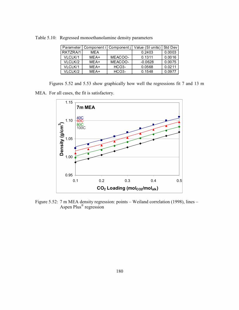
180

Table 5.10: Regressed monoethanolamine density parameters

Parameter Component i Component j Value (SI units) Std Dev

RKTZRA/1 MEA 0.2403 0.0003

VLCLK/1 MEA+ MEACOO- 0.1311 0.0016

VLCLK/2 MEA+ MEACOO- -0.0628 0.0075

VLCLK/1 MEA+ HCO3- 0.0568 0.0211

VLCLK/2 MEA+ HCO3- 0.1548 0.0977

Figures 5.52 and 5.53 show graphically how well the regressions fit 7 and 13 m

MEA. For all cases, the fit is satisfactory.

7m MEA

0.95

1.00

1.05

1.10

1.15

0.1 0.2 0.3 0.4 0.5


Density (g/cm

3)

40C60C80C100C

Figure 5.52: 7 m MEA density regression: points – Weiland correlation (1998), lines – Aspen Plus

® regression

181

13m MEA

0.95

1.00

1.05

1.10

1.15

1.20

0.1 0.2 0.3 0.4 0.5


Density (g/cm

3) 60C

40C

80C100C

Figure 5.53: 13 m MEA density regression: points – Weiland correlation (1998), lines – Aspen Plus

® regression

5.3.6.2 Viscosity

Monoethanolamine viscosity data for the regression were obtained from Weiland

(1998) correlations. MEA viscosity values were calculated for 7, 9, 11, and 13 m MEA

at 40, 60, 80, and 100˚C with loadings ranging from 0.2 to 0.5 at 0.05 increments.

Viscosity values for nonionic species are determined using the DIPPR liquid

viscosity model. The Jones-Dole electrolyte model is used to account for the viscosity

contributions of the ionic species. Table 5.11 summarizes the regressed viscosity

parameters for the MEA system. Figures 5.54 and 5.55 show how well the regression

matched the 7 and 13 m MEA data.

182

Table 5.11: Regressed monoethanolamine viscosity parameters

Parameter Component i Value (SI units) Std Dev

IONMUB/1 MEA+ -23.57 4.09

IONMUB/1 MEACOO- 24.13 4.09

MULDIP/1 MEA -43.21 3.38

MULDIP/2 MEA 13411 1087

7m MEA

0.1

1

10

0.20 0.25 0.30 0.35 0.40 0.45 0.50


Viscosity (cP)

40C

60C

80C

100C

Figure 5.54: 7 m MEA viscosity regression: points – Weiland correlation (1998), lines – Aspen Plus

® regression

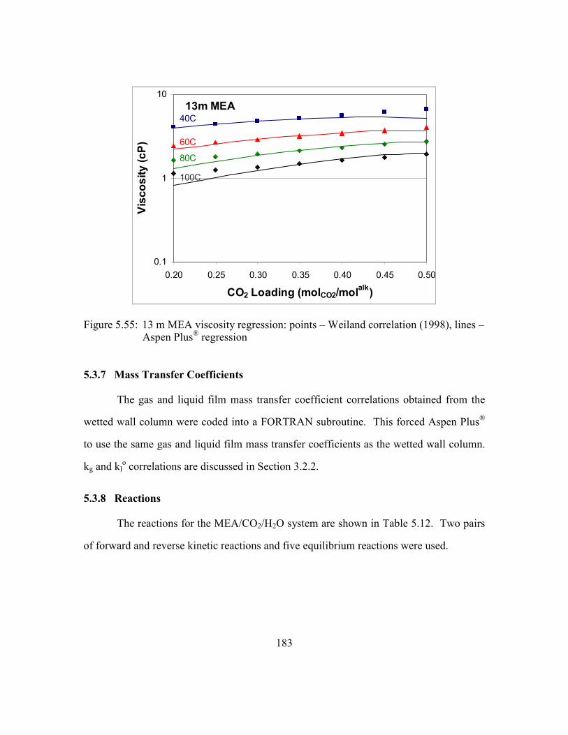
183

13m MEA

0.1

1

10

0.20 0.25 0.30 0.35 0.40 0.45 0.50


Viscosity (cP) 60C

40C

80C

100C

Figure 5.55: 13 m MEA viscosity regression: points – Weiland correlation (1998), lines – Aspen Plus

® regression

5.3.7 Mass Transfer Coefficients

The gas and liquid film mass transfer coefficient correlations obtained from the

wetted wall column were coded into a FORTRAN subroutine. This forced Aspen Plus®

to use the same gas and liquid film mass transfer coefficients as the wetted wall column.

kg and klo correlations are discussed in Section 3.2.2.

5.3.8 Reactions

The reactions for the MEA/CO2/H2O system are shown in Table 5.12. Two pairs

of forward and reverse kinetic reactions and five equilibrium reactions were used.

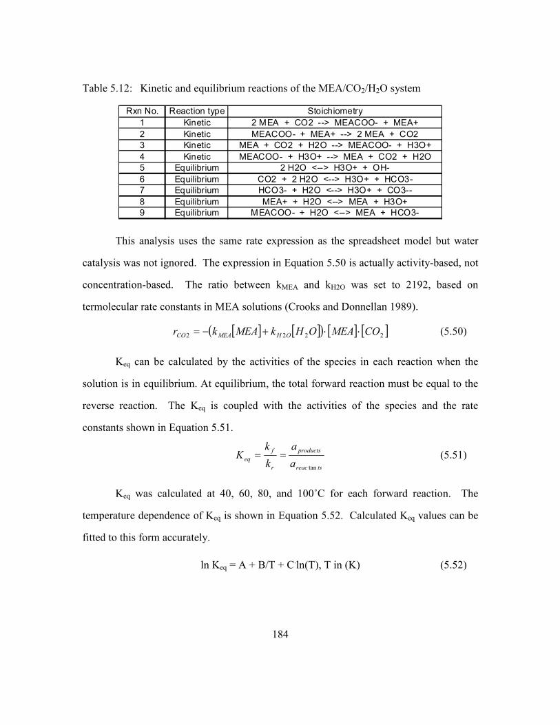
184

Table 5.12: Kinetic and equilibrium reactions of the MEA/CO2/H2O system

Rxn No. Reaction type Stoichiometry

1 Kinetic 2 MEA + CO2 --> MEACOO- + MEA+

2 Kinetic MEACOO- + MEA+ --> 2 MEA + CO2

3 Kinetic MEA + CO2 + H2O --> MEACOO- + H3O+

4 Kinetic MEACOO- + H3O+ --> MEA + CO2 + H2O

5 Equilibrium 2 H2O <--> H3O+ + OH-

6 Equilibrium CO2 + 2 H2O <--> H3O+ + HCO3-

7 Equilibrium HCO3- + H2O <--> H3O+ + CO3--

8 Equilibrium MEA+ + H2O <--> MEA + H3O+

9 Equilibrium MEACOO- + H2O <--> MEA + HCO3-

This analysis uses the same rate expression as the spreadsheet model but water

catalysis was not ignored. The expression in Equation 5.50 is actually activity-based, not

concentration-based. The ratio between kMEA and kH2O was set to 2192, based on

termolecular rate constants in MEA solutions (Crooks and Donnellan 1989).

[ ] [ ]( ) [ ] [ ]2222 COMEAOHkMEAkr OHMEACO ⋅⋅+−= (5.50)

Keq can be calculated by the activities of the species in each reaction when the

solution is in equilibrium. At equilibrium, the total forward reaction must be equal to the

reverse reaction. The Keq is coupled with the activities of the species and the rate

constants shown in Equation 5.51.

tsreac

products

r

f

eqa

a

k

kK

tan

== (5.51)

Keq was calculated at 40, 60, 80, and 100˚C for each forward reaction. The

temperature dependence of Keq is shown in Equation 5.52. Calculated Keq values can be

fitted to this form accurately.

ln Keq = A + B/T + C.ln(T), T in (K) (5.52)

185

Aspen Plus® uses a power law rate expression, as shown in Equation 5.53, where

k is the pre-exponential constant, T is the temperature, T0 is a reference temperature, EA

is the activation energy, and R is the gas constant.

−

−

=

00

11exp

TTR

E

T

Tkr a

n

(5.53)

The equilibrium constant form relates to the power law rate expression. The A in

the Keq expression can be related to the rate constant while B and C can be related to Ea/R

and n, respectively. A simple equation can be implemented inside a design specification

in the model to ensure that the reverse rate expression is always thermodynamically

consistent with the forward rate expression.

The activation energy was input as 44.9 kJ/mol, based on the value reported by

Versteeg (1996). The reference temperature is 298.15 K. Fitting the rate constant to the

data produced a value of 6.1x106 for the MEA catalysis reaction.

5.3.9 Model Results

Figures 5.56–5.58 show the error in the flux with respect to the MEA

concentration, CO2 loading, and temperature. The final model balances the negative and

positive flux errors by adjusting the rate constant until the sum of the squares of the errors

was minimized. The final pre-exponential rate constant obtained was 6.1·106 based on

the form of Equation 5.53.

∑

−2

mod

meas

measel

Flux

FluxFlux (5.54)

Not all the wetted wall column conditions have been plotted in Figures 5.56–5.58.

Some conditions introduce large, expected errors so they were excluded from the

analysis. Data points at the highest CO2 loading, near 0.5, were excluded because the

186

model cannot accurately predict the correct free amine concentration after the CO2

loading is adjusted to fit the partial pressure data. The 0.46 CO2 loading data for 11 m

MEA were retained in the analysis. At each experimental condition, six inlet CO2 partial

pressures were tested in the wetted wall column. This analysis only includes highest and

lowest of the six inlet CO2 partial pressures. Any points that had inlet CO2 partial

pressures within 25% of the equilibrium partial pressure were excluded. Also, 7 m MEA,

60˚C at 0.252 loading; 7 m MEA, 100˚C at 0.271 CO2 loading; and 9 m MEA, 60˚C at

0.231 CO2 loading were excluded from this analysis. Each of these conditions presented

large changes in CO2 loading when the partial pressure was matched. These errors

resulted from a flattening of the CO2 partial pressure curve at low CO2 loading. The

remaining wetted wall column conditions are examined in Figures 5.56–5.58.

-0.50

0.00

0.50

6 8 10 12 14

Total MEA Concentration (m)

(Nmodel-Nmeas)/Nmeas

40C 60C

80C 100C

Figure 5.56: Aspen Plus® RateSep™ model error against total MEA concentration for

wetted wall column experimental conditions

187

-0.50

0.00

0.50

0.20 0.25 0.30 0.35 0.40 0.45 0.50



7m MEA 9m MEA

11m MEA 13m MEA

Figure 5.57: Aspen Plus® RateSep™ model error against CO2 loading for wetted wall

column experimental conditions

-0.50

0.00

0.50

30 40 50 60 70 80 90 100 110

Temperature (C)


7 m MEA 9 m MEA

11 m MEA 13 m MEA

Figure 5.58: Aspen Plus® RateSep™ model error against temperature for wetted wall

column experimental conditions

188

Errors in the flux calculated by the model are always within 50% of the wetted

wall column measured fluxes. This is acceptable considering the magnitude of the flux

varies about a factor of 100. Absorption and desorption runs are both considered. Model

errors seem to spread evenly with changes in CO2 loading and temperature. There is a

significant systematic error in the predicted flux with changes in amine concentration.

The MEA model has a flaw in its ability to predict flux with changing MEA

concentration because of an inability to regress MEA activity coefficients accurately.

Figure 5.2, utilizing MEA volatility data from Hilliard (2008), showed that the MEA

activity coefficient was independent of amine concentration. The spreadsheet model

showed no systematic trend with MEA concentration, suggesting that MEA dependent

parameters in the kg’ rate expression (Equation 5.48) are correct. Although the MEA

volatility data had three times the emphasis of other data in the main MEA regression, the

model still showed significant MEA concentration dependences in the MEA activity

coefficient. Figure 5.59 includes the same conditions as Figure 5.2 but the activity

coefficients are from the model rather than the modified Raoult’s law equation.

189

Model Predictions

0.4

0.6

0.8

1.0

0.1 0.2 0.3 0.4 0.5 0.6



7 m MEA, 40C

11 m MEA, 40C

3.5 m MEA, 40C

Figure 5.59: Aspen Plus® RateSep™ model prediction of MEA activity coefficients at

MEA volatility experiment conditions tested by Hilliard

The increasing activity coefficient with increasing MEA concentration ensures

that the model under-predicts rates at low MEA concentrations while overpredicting CO2

mass transfer rates at the highest MEA concentrations.

Due to the limitation in representing the MEA activity coefficient, the RateSep™

model is most accurate when fine-tuned to one specific amine concentration. The error in

the predicted flux seems to be about 25% for each amine concentration.

190

Chapter 6: Conclusions and Recommendations

This chapter is separated into 3 parts. The scope and methods state the tasks that

were performed. The conclusions summarize the results and detail what was learned

from this work. The recommendations provide suggestions and recommendations for

future work.

6.1 SCOPE AND METHODS

Diffusion experiments were carried out in a diaphragm cell for 7, 9, and 13 m

MEA and 2, 5, and 8 m PZ at 30˚C. Each experiment used solutions with a different CO2

loading on each side of the glass frit. Changes in CO2 loading were detected using

density measurements. Measured changes in density are much more accurate than

measured changes in CO2 loading using the inorganic carbon analyzer. The membrane-

cell integral diffusion coefficient, D , was correlated with the viscosity of the amine

solutions.

Wetted wall column experiments were conducted for 7, 9, 11, and 13 m MEA and

2, 5, 8, and 12 m PZ solutions. 7 m MEA/2 m PZ solutions were also tested.

Experiments were performed at 40, 60, 80, and 100˚C. Generally, four CO2 loadings

were tested at 40 and 60˚C and two CO2 loadings were tested at 80 and 100˚C. The

wetted wall column can only measure CO2 equilibrium partial pressures up to about

40 kPa, due to the maximum range of the available CO2 analyzers. A total of 105 wetted

wall column experiments were performed, each testing six inlet CO2 partial pressures.

191

Each wetted wall column experiment obtained the equilibrium CO2 partial pressure of the

solution and the liquid film mass transfer coefficient, kg’. kg’, not the rate constant, is the

definitive measure of the reaction rate of an amine solution.

Spreadsheet modeling was performed for both MEA and PZ solutions. A rate

expression and an expression for kg’ were developed from the experimental data. Each of

the parameters in the kg’ expression was estimated based on literature data. Parameters

that lacked literature data were estimated by extrapolating related data. The spreadsheet

model was able to detail exactly how parameters in the kg’ expression and kg’ are affected

by changes in temperature, CO2 loading, and amine concentration.

An Aspen Plus® RateSep™ model was created for MEA systems based on the

spreadsheet model and wetted wall column data. This model predicts CO2 flux based on

operating conditions. It can be scaled to industrial conditions to predict CO2 mass

transfer characteristics.

6.2 CONCLUSIONS

6.2.1 Diaphragm Cell Experiments

Diffusion coefficients in MEA and PZ vary to the 0.72±0.12 power of viscosity.

This value was obtained by measuring diffusion coefficients in 7, 9, and 13 m MEA and

2, 5, and 8 m PZ at 30˚C over a wide range of CO2 loading. Literature generally reports

diffusion coefficients that vary to the 0.8 power of viscosity for N2O and the 0.6 power

for amine solutes (Versteeg and Van Swaaij 1988; Snijder, te Riele et al. 1993). The 0.72

power of viscosity is based on the measured membrane-cell integral diffusion coefficient,

D , which is a complex concentration and time-averaged value, different from the

fundamental diffusion coefficient, D.

192

The diffusion coefficient-viscosity curve for MEA and PZ solutions extrapolates

favorably to the reported diffusion coefficient of 1 M PZ (Sun, Yong et al. 2005).

The spreadsheet models implement a 0.72 power of viscosity on the diffusion

coefficient.

6.2.2 Wetted Wall Column Experiments

MEA solutions below 0.45 CO2 loading and all tested PZ solutions (0.21–0.41

CO2 loading) exhibit equilibrium CO2 partial pressures independent of amine

concentration. The partial pressure is strictly a function of the temperature and CO2

loading for each system. Wetted wall column experiments and Hilliard (2008) both show

an effect of total MEA concentration at very high loading. Aqueous MEA at high CO2

loading exhibits increasing CO2 partial pressures with increasing amine concentration.

Near 0.5 CO2 loading, bicarbonate should be present in significant concentrations.

Theory suggests that the CO2 equilibrium partial pressure should be independent of total

amine concentration for carbamate production but not for bicarbonate production

(Appendix D).

CO2 equilibrium partial pressures measurement from the wetted wall column in

MEA, PZ, and MEA/PZ match literature data very well (Jou, Mather et al. 1995;

Ermatchkov, Perez-Salado Kamps et al. 2006a; Hilliard 2008). Only the 40˚C MEA

experiments at the highest CO2 loading seem to deviate from the literature data. Hilliard

(2008) shows the same trend, where higher amine concentration solutions have higher

CO2 partial pressures. However, the measured equilibrium partial pressures at 40˚C do

not match the magnitude of the Hilliard (2008) and Jou (1995) measurements.

193

8 m PZ exhibits a 70% greater CO2 capacity than 7 m MEA and a 50% greater

CO2 capacity than 11 m MEA. The CO2 capacity is the difference in CO2 concentrations

between lean and rich solutions, the amount of CO2 removed from the system per unit of

solvent. The majority of the increased CO2 capacity is due to the fact that each mole of

piperazine has two functional nitrogen groups. This allows PZ to react twice in the CO2

reaction, whereas MEA can only react once. Over the 5000–100 Pa operating range at

40˚C, 7 m MEA, 11 m MEA, and 8 m PZ have CO2 capacities of 0.85, 0.93, and

1.41 molCO2/kg(water+amine).

The liquid film mass transfer coefficient, kg’, in aqueous MEA is essentially

independent of temperature and the total amine concentration in the wetted wall column.

The CO2 loading of the solution dictates kg’. kg’ varies about a factor of 30 in aqueous

MEA with 0.23–0.50 CO2 loading. The decreased rate is primarily due to the decrease in

free amine concentration at higher CO2 loading.

kg’ in aqueous PZ is independent of temperature and total amine concentration at

lower temperatures and constant CO2 loading in the wetted wall column. 100˚C data

points fall below the other kg’ values at low and intermediate CO2 loadings. At

intermediate CO2 loadings, the drop in the 100˚C rate data is more pronounced. At

intermediate CO2 loading, 80˚C kg’ values also drop below those at lower temperatures.

60˚C kg’ values fall slightly below the 40˚C kg’ values at the highest CO2 loadings. kg’

ranges about a factor of 20 in aqueous PZ with 0.21–0.41 CO2 loading.

A drop in kg’ at higher temperature and CO2 loading is not unexpected, especially

for PZ, since it is the faster reacting amine. High temperature and CO2 loading

conditions should encounter more diffusion resistance due to less free amine and a

greater slope of the equilibrium line. Diffusion resistances in wetted wall column

194

experiments with MEA are typically minor. This is not the case for the faster reacting PZ

solutions in the wetted wall column. When diffusion resistances become significant, kg’

becomes apparatus dependent. The wetted wall column has a 9.1 cm contactor which

produces a 9.1 cm laminar flow path. Amine solutions in either structured or random

packed columns will have laminar flow paths significantly shorter than 9.1 cm, yielding

larger physical mass transfer coefficients. Industrial columns should not exhibit these

drastic drops in kg’ with increasing temperature and CO2 loading.

Experimental results show that PZ is 2–3 times faster than MEA. This means that

to a first approximation 1/2 to 2/3 less column packing would be required for PZ

compared to MEA. Both MEA and PZ rate data match well with applicable literature

data.

6.2.3 Modeling

6.2.3.1 Spreadsheet Modeling

Wetted wall column experiments show that CO2 reaction rates in both aqueous

MEA and PZ are second order in amine when presented on an activity basis. These

activity-based rate expressions were implemented into shell balance equations to produce

pseudo first order rate expressions. Implementing diffusion resistances into the pseudo

first order rate expressions using film theory provides the following kg’ expressions for

MEA and PZ solutions.

[ ]

∆

∆+=

T

o

COMEA

OHCOCO

gCO

P

kDMEAk

H

k

CO

prodl 2

*

2

22

2,2

5.0

2

'

2

,

1

][

1

γ

γ (6.1)

195

[ ] [ ] [ ][ ] [ ][ ]

[ ]

∆

∆+

+

+

+=

−

−

−T

o

CO

PZCOOPZCOO

PZPZCOOPZCOO

PZCOOPZPZPZPZ

OHCOCO

gCO

P

k

D

PZCOOk

PZPZCOOk

PZCOOPZkPZk

H

k

CO

prodl2

*

2

22

22

2,2

5.0

2

'

2

,

11

γ

γγ

γγγ

γ (6.2)

Each parameter in Equations 6.1 and 6.2 was estimated from literature data. In

some cases, literature data could not be used and assumptions were required. The activity

coefficient of MEA was obtained from MEA volatility data (Hilliard 2008). The activity

coefficients of PZ and PZCOO– were obtained from the thermodynamic model of Hilliard

(2008). Free MEA, PZ, and PZCOO– concentrations were also obtained from the Hilliard

model (2008). The activity coefficient of CO2 in both MEA and PZ solutions was

obtained from N2O solubility data in MEA (Browning and Weiland 1994; Hartono 2009).

In the case of PZ, the CO2 loading in the CO2 solubility equation was multiplied by two

to make the equation a better indicator of the total CO2 concentration. The diffusion

coefficient of CO2 was obtained from a DCO2 correlation in water (Versteeg, Van Dijck et

al. 1996) in conjunction with 0.72 viscosity exponent obtained using diaphragm diffusion

cell experiments. The Henry’s solubility of CO2 in water was obtained by correlating

literature data (Versteeg and Van Swaaij 1988). The liquid phase mass transfer

coefficient of the reactants and products, 0

, prodlk , was calculated using a theoretical model

by Pigford (1941). The slope of the equilibrium line was obtained by taking the

derivative of the CO2 partial pressure expressions developed by Xu (Rochelle, Chen et al.

2009b). PZCOO– rate constants were set to 70% of the value of the PZ rate constant

based on work by Cullinane (2006). The temperature dependence of the MEA rate

constant was obtained from a review of literature data (Versteeg, Van Dijck et al. 1996).

The temperature dependence of the PZ rate constant was obtained from Cullinane (2006).

The pre-exponential value in kMEA and kPZ were adjusted to fit the experimental data.

196

These two pre-exponential rate constants and the assertion of termolecular kinetics are

the only parameters that were adjusted to match experimental data. Experimental trends

with CO2 loading, amine concentration, or temperature cannot be fitted by these adjusted

parameters. These trends are predicted by the estimated parameters in Equations 6.1 and

6.2.

The literature-based parameter estimations in Equations 6.1 and 6.2 account for

the offsetting temperature and amine concentration effects on kg’. These trends are

predicted by the literature data, not fitted by the model.

Equation 6.1 represents the measured kg’ in aqueous MEA with an average error

of 13%. Equation 6.2 represents the measured kg’ in aqueous PZ with an average error of

19%. The kg’ representations are excellent considering kg’ can vary up to a factor of 20–

30 over the range of experimental conditions. Since the kg’ representations are accurate,

the representation of each of the parameters in Equations 6.1 and 6.2 are likely accurate.

The determination of kg’ has been fully explained in both MEA and PZ systems using

literature data to estimate the parameters in Equation 6.1 and 6.2. Other amine systems

can likely be explained similarly.

6.2.3.2 Aspen Plus® RateSep™ Modeling

An Aspen Plus® RateSep™ model was created to model the CO2 flux for 7-13 m

MEA systems. The absorber/stripper model consists of a single column based on the

wetted wall column. The model makes use of the sequential regression technique and

regressed binary system parameters from Hilliard (2008). Parameters for the tertiary

system (MEA/H2O/CO2) were re-regressed with updated data and fewer regressed

parameters.

197

The main MEA data regression succeeds in accurately predicting CO2 partial

pressure in 7 m MEA. At higher MEA concentrations, the fit get progressively worse.

The CO2 loading of inlet conditions was adjusted to produce an exact match to the wetted

wall column measured equilibrium partial pressure. The error introduced by changing

the free amine concentration is much smaller than the error introduced by having

erroneous driving forces.

Parameters that control the CO2 activity coefficient in the solution were manually

adjusted to produce values that mimic the CO2 solubility expression (Equation 5.11)

based on literature data (Browning and Weiland 1994; Hartono 2009).

The gas and physical liquid film mass transfer coefficient correlations used for the

wetted wall column were coded into a FORTRAN subroutine. This causes Aspen Plus®

to use the same gas and liquid film mass transfer coefficients as the wetted wall column.

Two pairs of forward and reverse kinetic reactions and five equilibrium reactions

were used in the model. The forward rate constants were dynamically linked to each

other based on a termolecular evaluation (Crooks and Donnellan 1989). The reverse

reaction rates were dynamically linked to the forward rate expressions using design

specifications to ensure that the equilibrium constant, Keq, is not violated. The lone

independent rate constant was adjusted until the model matched wetted wall column

results.

Overall, the model predicts the CO2 flux within about 40%. The model does not

properly account for the MEA activity coefficient with changing amine concentration.

This introduces error with changing amine concentration. At each amine concentration

the fit can be improved to about ±25%.

198

6.3 RECOMMENDATIONS

The diaphragm diffusion cell experiments are not as accurate as desired. These

experiments also take a significant amount of time, about two weeks each. Experiments

at very viscous conditions, such as 12 m PZ, failed and were not reported. Another

method to determine diffusion coefficients, such as the Taylor dispersion method used by

Hamborg (2008), should prove more accurate and much faster. This technique would

allow for the measurement of N2O over a much wider range of conditions with greater

accuracy.

One weakness in the PZ spreadsheet model is the representation of the PZ and

PZCOO– activity coefficients. Results from the Hilliard (2008) model were used.

Although the model properly represents the PZ data, more confidence could be placed in

amine activity coefficients if these parameters could be directly supported by literature

data. Maybe some experiments can be designed to quantify PZ and PZCOO– activity

coefficients.

Another weakness of the PZ spreadsheet model deals with the physical solubility

of CO2 in aqueous PZ. The model assumed a similar behavior to MEA because no data

has been published for N2O solubility in concentrated, CO2 loaded piperazine solutions.

N2O solubility experiments in PZ and other amine solutions would be useful. Ideally,

these experiments would include high amine concentrations at wide temperature ranges

and relevant CO2 loading.

The Aspen Plus® RateSep™ model was unable to produce MEA activity

coefficients independent of the total amine concentration. This inability introduces

inaccuracies at varying amine concentrations. More flexibility or a workaround in Aspen

Plus® to solve this problem would be useful.

199

From a rate and capacity perspective, PZ is a much better solvent than MEA. A

comprehensive study should be performed to see if using concentrated PZ (5–8 molal)

would produce significant energy and capital cost savings in a CO2 capture system.

200

Appendix A: Nomenclature

This appendix includes all the shorthand nomenclature used throughout the

dissertation. The nomenclature is organized alphabetically. Greek symbols are included

at the end.

* equilibrium

A gas-liquid contact area

alk alkalinity

Am amine

[Am]b concentration of amine in the bulk solution

AMP 2-amino-2-methyl-l-propanol

b bulk

B base

C celsius

cP centipoise

d hydraulic diameter (outside diameter minus inside diameter)

D membrane-cell integral diffusion coefficient

DCO2 diffusion coefficient of CO2

201

DEA diethanolamine

DGA diglycolamine

e equilibrium

FTIR Fourier transform infrared spectroscopy

g gravity

h hour

h height

HCO2 Henry’s constant – CO2 solubility in solution

HCO2,H2O Henry’s constant – CO2 solubility in water

HCO3– bicarbonate

i interface

IR infrared

k rate constant

K Kelvin

Ka equilibrium constant of acid dissociation with water

kb rate constant of the base protonation

kf forward rate constant

kg kilogram

KG overall mass transfer coefficient (gas phase units)

kg gas film mass transfer coefficient

202

kg’ liquid film mass transfer coefficient (gas phase units)

kg’’ pseudo first order liquid film mass transfer coefficient (gas phase

units)

kH2O rate constant of water protonation

kl liquid film mass transfer coefficient

klo liquid film physical mass transfer coefficient

kMEA rate constant of MEA protonation

kPa kilopascal

kr reverse rate constant

l liter

Ldg CO2 loading

lm log mean

m molality (mol/kg water)

m meter

M molarity (mol/l solution)

Mb molecular weight of component b

MDEA methyldiethanolamine

MEA monoethanolamine

min minute

mol mole

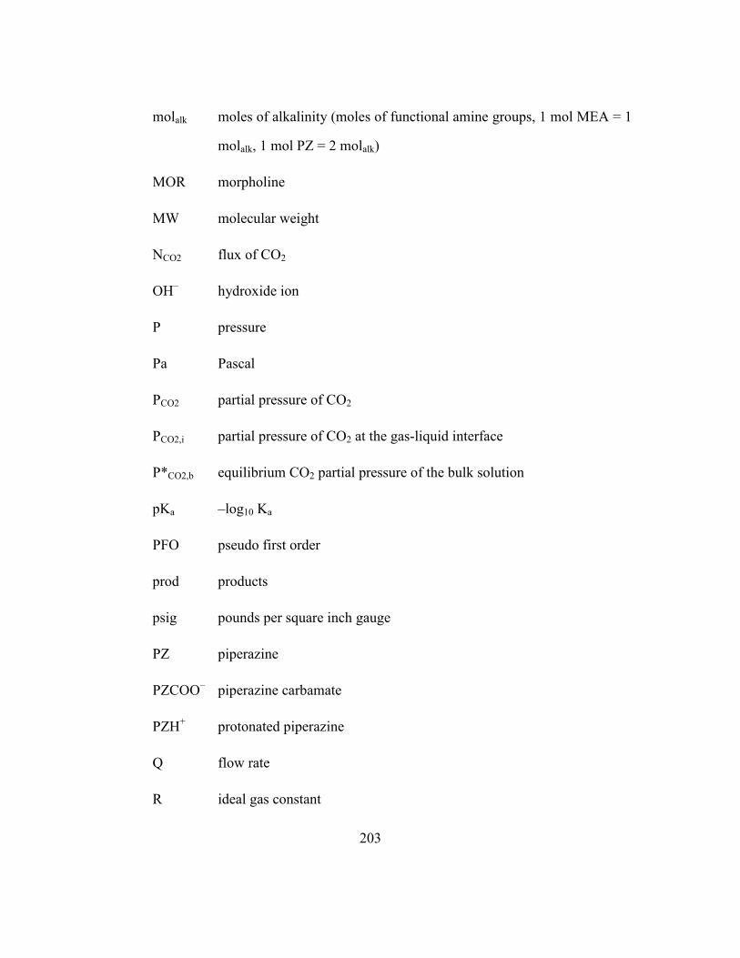
203

molalk moles of alkalinity (moles of functional amine groups, 1 mol MEA = 1

molalk, 1 mol PZ = 2 molalk)

MOR morpholine

MW molecular weight

NCO2 flux of CO2

OH– hydroxide ion

P pressure

Pa Pascal

PCO2 partial pressure of CO2

PCO2,i partial pressure of CO2 at the gas-liquid interface

P*CO2,b equilibrium CO2 partial pressure of the bulk solution

pKa –log10 Ka

PFO pseudo first order

prod products

psig pounds per square inch gauge

PZ piperazine

PZCOO– piperazine carbamate

PZH+ protonated piperazine

Q flow rate

R ideal gas constant

204

rCO2 rate of CO2 formation

RDint reaction-diffusion interface

Re Reynolds number

s second

Sc Schmidt number

Sh Sherwood number

St stokes

t time

T temperature

T total

Tref reference temperature

u velocity

Va molar volume of component A

W circumference

wt% weight percent

x nominal rotameter reading

xMEA liquid mole fraction of MEA

yMEA gas mole fraction of MEA

205

Greek symbols

α CO2 loading

β cell constant

γ activity coefficient

δ film thickness

η viscosity

η dimensionless penetration distance

Θ dimensionless driving force

µ viscosity

ρ density

Ψ association parameter in Wilke-Chang equation

ω mass fraction amine

Ω mass percentage of the amine

206

Appendix B: Detailed Diaphragm Cell Data

This appendix includes all the data from the diaphragm cell experiments required

to recalculate the membrane-cell integral diffusion coefficient, D . The initial CO2

loading and measured density at 20˚C are shown for the solutions in the top and bottom

chambers of the cell. The final density was measured at 20˚C after conclusion of the

experiment. Assuming a linear density-CO2 loading relationship, justified by density

measurements by Freeman (Rochelle, Dugas et al. 2008), the final CO2 loading was

calculated. Table B.1 also includes the cell constant. Two different diaphragm cells

were used in the experiments. Each was calibrated with a KCl solution to determine the

cell constant.

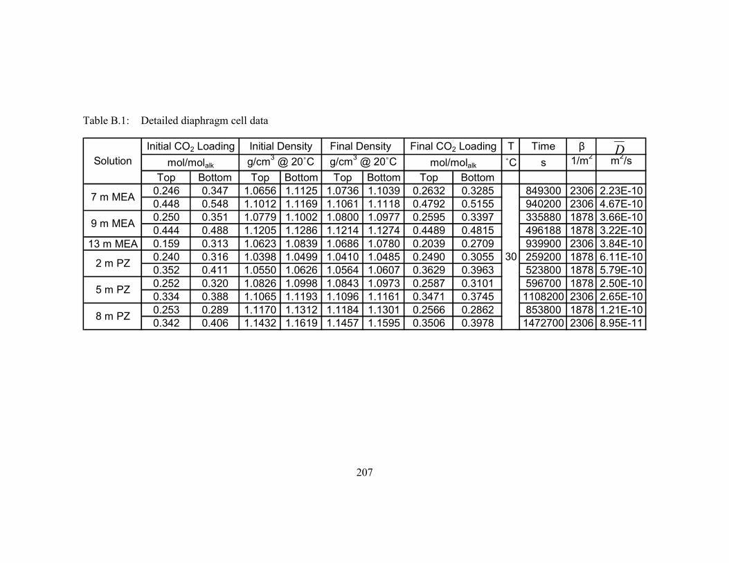
207

Table B.1: Detailed diaphragm cell data

T Time β

˚C s 1/m2

m2/s

Top Bottom Top Bottom Top Bottom Top Bottom

0.246 0.347 1.0656 1.1125 1.0736 1.1039 0.2632 0.3285 849300 2306 2.23E-10

0.448 0.548 1.1012 1.1169 1.1061 1.1118 0.4792 0.5155 940200 2306 4.67E-10

0.250 0.351 1.0779 1.1002 1.0800 1.0977 0.2595 0.3397 335880 1878 3.66E-10

0.444 0.488 1.1205 1.1286 1.1214 1.1274 0.4489 0.4815 496188 1878 3.22E-10

13 m MEA 0.159 0.313 1.0623 1.0839 1.0686 1.0780 0.2039 0.2709 939900 2306 3.84E-10

0.240 0.316 1.0398 1.0499 1.0410 1.0485 0.2490 0.3055 259200 1878 6.11E-10

0.352 0.411 1.0550 1.0626 1.0564 1.0607 0.3629 0.3963 523800 1878 5.79E-10

0.252 0.320 1.0826 1.0998 1.0843 1.0973 0.2587 0.3101 596700 1878 2.50E-10

0.334 0.388 1.1065 1.1193 1.1096 1.1161 0.3471 0.3745 1108200 2306 2.65E-10

0.253 0.289 1.1170 1.1312 1.1184 1.1301 0.2566 0.2862 853800 1878 1.21E-10

0.342 0.406 1.1432 1.1619 1.1457 1.1595 0.3506 0.3978 1472700 2306 8.95E-11

30

5 m PZ

8 m PZ

mol/molalk

Initial CO2 Loading

Solution

7 m MEA

9 m MEA

2 m PZ

Initial Density

g/cm3 @ 20˚C

Final Density Final CO2 Loading

mol/molalkg/cm3 @ 20˚C

D

208

Appendix C: Detailed Wetted Wall Column Data

This appendix includes all the relevant data obtained from the wetted wall column

experiments. The following tables include amine concentration, CO2 loading,

equilibrium CO2 partial pressure, temperature, pressure, gas and liquid flow rates,

equilibrium inlet and outlet CO2 partial pressures, and mass transfer coefficients. KG/kg

represents the fractional gas film resistance of the experiment. Experiments were

designed be less than 50% gas film controlled. The following tables also include the

solvent flow rate and o

prodlk

,.

For aqueous MEA, density and viscosity correlations, required to calculate the

liquid flow rate and physical liquid film mass transfer coefficient, were obtained from

Weiland (1998). The Weiland correlations are valid up to 40 wt% amine, 0.6 CO2

loading, and 120˚C. 13 m MEA data (44.3 wt%) are extrapolated.

Piperazine density data was obtained by regressing 2–12 m PZ density

measurements at 20, 40, and 60˚C from Freeman (Rochelle, Chen et al. 2009a). PZ

solution viscosity values were obtained by regressing 5–12 m PZ viscosity measurements

at 25, 40, and 60˚C from Freeman (Rochelle, Sexton et al. 2008a). Details on the PZ

density and viscosity regressions are included in Appendix E.

MEA/PZ density and viscosity data have not been compiled into density and

viscosity regressions. 7 m MEA/2 m PZ solutions were assumed to follow the Weiland

(1998) density predictions for 37.5 wt% MEA. 7 m MEA/2 m PZ solutions are 37.5 wt%

209

amine. No attempt has been made to estimate 7 m MEA/2 m PZ viscosities at wetted

wall column experimental conditions. Therefore, o

prodlk

,has not been calculated.

210

Table C.1: Detailed wetted wall column data – 7 m MEA

MEA CO2 Ldg P*CO2 Temp Pres GasDry Gas Liquid PCO2,in,dry PCO2,in,wet PCO2,out,dry PCO2,out,wet kol,prod CO2 Flux KG kg KG/kg kg'

m mol/molalk Pa C psig Std l/min Std l/min ml/s Pa Pa Pa Pa m/s mol/s.m

2mol/s

.Pa

.m

2mol/s

.Pa

.m

2mol/s

.Pa

.m

2

0 0 6 6 -2.42E-05

10 10 12 12 -9.28E-06

20 19 19 19 3.23E-06

30 29 24 23 2.42E-05

40 39 31 30 3.55E-05

50 48 38 37 4.96E-05

0 0 20 19 -8.07E-05

60 58 65 63 -2.02E-05

120 116 109 106 4.44E-05

180 174 154 149 1.05E-04

240 233 204 198 1.45E-04

300 291 252 244 1.94E-04

0 0 105 103 -2.46E-04

200 196 262 257 -1.45E-04

400 393 413 406 -3.05E-05

600 589 570 560 7.04E-05

800 786 730 717 1.64E-04

1000 982 885 869 2.70E-04

800 789 1300 1281 -9.37E-04

1600 1577 1995 1966 -7.41E-04

2400 2366 2665 2627 -4.97E-04

3200 3154 3370 3322 -3.19E-04

4000 3943 4025 3967 -4.69E-05

5000 4928 4900 4830 1.87E-04

0 0 43 39 -1.74E-04

60 55 79 72 -7.67E-05

120 110 117 107 1.21E-05

180 165 158 145 8.88E-05

240 220 200 183 1.61E-04

300 275 240 220 2.42E-04

0 0 175 160 -7.06E-04

300 275 405 371 -4.24E-04

600 550 635 582 -1.41E-04

900 825 855 784 1.82E-04

1200 1100 1080 990 4.84E-04

1500 1375 1305 1196 7.87E-04

7

7

7

7

7

7

0.252

0.351

0.432

0.496

0.252

0.351

3.34E-06

1.40E-06

7.66E-07

3.47E-07

0.42

0.23

0.23

0.14

2.63E-06

2.09E-06

2.92E-06

1.70E-06

0.38

0.264.83E-06

4.1E-05

1.26E-06

4.4E-05

5.9E-05

5.7E-05

1.07E-06

5.93E-07

3.2

3.1 4.2E-05

5.0

5.16

5.09

4.83E-06

1.93E-064.6E-05

2.98E-07

1.82E-06

4.57E-06

4.57E-06

5.07

5.45

5.45

3.25.16

3.2

3.2

3.1

204015.7

77 40 20

465

4216

109

660

40

40

60

60

20

20

5.0

5.0

5.0

5.0

5.0

60

45

211




2mol/s

.Pa

.m

2mol/s

.Pa

.m

2mol/s

.Pa

.m

2

0 0 890 847 -2.09E-03

1250 1189 1820 1732 -1.34E-03

2500 2379 2760 2626 -6.10E-04

3750 3568 3730 3549 4.69E-05

5000 4758 4660 4434 7.98E-04

6250 5947 5600 5329 1.52E-03

0 0 2500 2403 -4.69E-03

8000 7690 9250 8892 -2.34E-03

16000 15381 16250 15621 -4.69E-04

24000 23071 23000 22110 1.87E-03

32000 30761 29700 28550 4.31E-03

40000 38452 36400 34991 6.75E-03

0 0 410 339 -1.45E-03

300 248 640 529 -1.20E-03

600 496 845 699 -8.64E-04

900 744 1040 860 -4.94E-04

1200 992 1220 1009 -7.06E-05

1500 1240 1410 1166 3.17E-04

0 0 1470 1244 -4.61E-03

2000 1692 2970 2513 -3.04E-03

4000 3385 4450 3766 -1.41E-03

6000 5077 5800 4908 6.27E-04

8000 6770 7150 6051 2.66E-03

10000 8462 8600 7278 4.39E-03

0 0 2700 1974 -6.91E-03

4000 2925 5150 3766 -2.94E-03

8000 5850 7750 5667 6.40E-04

12000 8775 10450 7642 3.97E-03

16000 11700 12600 9214 8.71E-03

20000 14625 15100 11042 1.25E-02

0 0 7700 6076 -1.55E-02

7500 5918 12100 9548 -9.24E-03

15000 11837 17900 14125 -5.83E-03

22500 17755 23100 18228 -1.21E-03

30000 23673 27900 22016 4.22E-03

37500 29591 33600 26514 7.84E-03

0.432

2.85E-06

0.152.16E-063.20E-075.3E-05

5.045603434 5.4E-05 9.28E-07

3.76E-07

0.252.72E-066.92E-073.15.25

7

7

7

7

7

7

0.384.64E-061.77E-066.7E-052.86.055.0258010530.271

0.496 16157 60 60 5.0 5.20 3.1

5.0

5.0

5.0

30

5297 100 40

0.366

0.271

4443 80

0.366 19008 100 55 6.34 2.8 9.30E-07 2.77E-06 0.34

4.04E-06

8.2E-05

5.91 2.7 1.28E-06

6.84 2.8

1.40E-06

6.4E-05 0.32 1.87E-06

1.66E-06 3.76E-06 0.44 2.98E-068.7E-05

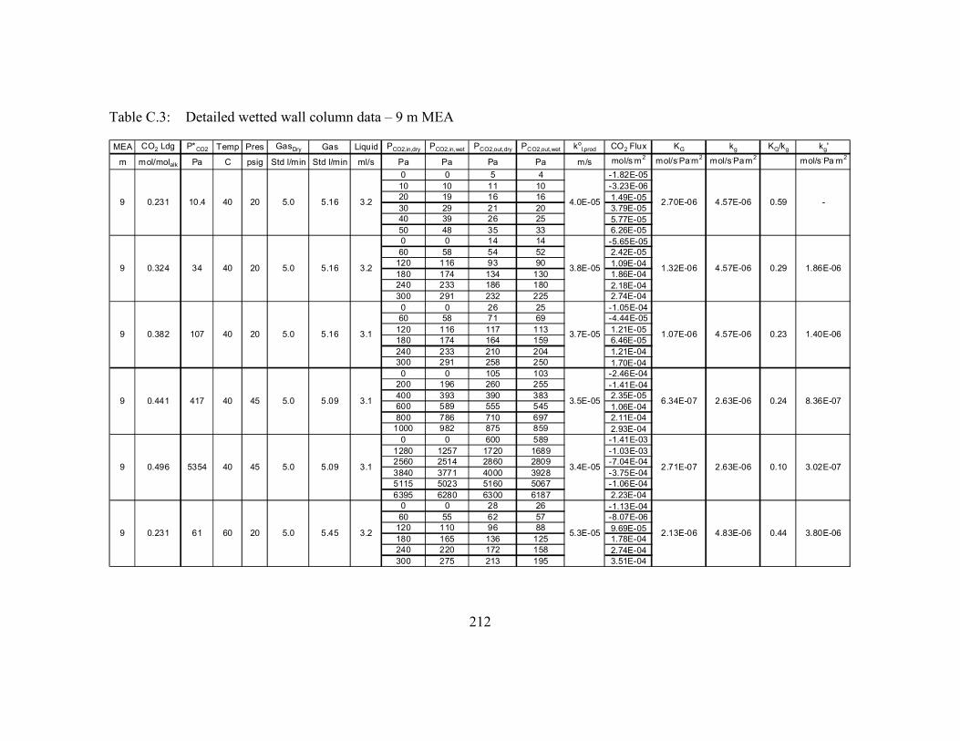
212




2mol/s

.Pa

.m

2mol/s

.Pa

.m

2mol/s

.Pa

.m

2

0 0 5 4 -1.82E-05

10 10 11 10 -3.23E-06

20 19 16 16 1.49E-05

30 29 21 20 3.79E-05

40 39 26 25 5.77E-05

50 48 35 33 6.26E-05

0 0 14 14 -5.65E-05

60 58 54 52 2.42E-05

120 116 93 90 1.09E-04

180 174 134 130 1.86E-04

240 233 186 180 2.18E-04

300 291 232 225 2.74E-04

0 0 26 25 -1.05E-04

60 58 71 69 -4.44E-05

120 116 117 113 1.21E-05

180 174 164 159 6.46E-05

240 233 210 204 1.21E-04

300 291 258 250 1.70E-04

0 0 105 103 -2.46E-04

200 196 260 255 -1.41E-04

400 393 390 383 2.35E-05

600 589 555 545 1.06E-04

800 786 710 697 2.11E-04

1000 982 875 859 2.93E-04

0 0 600 589 -1.41E-03

1280 1257 1720 1689 -1.03E-03

2560 2514 2860 2809 -7.04E-04

3840 3771 4000 3928 -3.75E-04

5115 5023 5160 5067 -1.06E-04

6395 6280 6300 6187 2.23E-04

0 0 28 26 -1.13E-04

60 55 62 57 -8.07E-06

120 110 96 88 9.69E-05

180 165 136 125 1.78E-04

240 220 172 158 2.74E-04

300 275 213 195 3.51E-04

9

9

9

9

9

9 5.0

5.0

5.0

5.0

5.0

5.0

0.231 10.4 40 20 5.16 3.2 4.0E-05 2.70E-06 4.57E-06 0.59 -

0.324 34 40 20 5.16 3.2 1.32E-06 4.57E-06 0.29 1.86E-06

0.382 107 40 20 5.16 3.1 1.07E-06 4.57E-06 0.23 1.40E-06

0.441 417 40 45 5.09 3.1 6.34E-07 2.63E-063.5E-05 0.24 8.36E-07

0.496 5354 40 45 5.09 3.1 2.71E-07 2.63E-06 0.10 3.02E-07

0.231 61 60 20 5.45 3.2 2.13E-06 4.83E-06 0.44 3.80E-06

3.8E-05

3.7E-05

3.4E-05

5.3E-05

213




2mol/s

.Pa

.m

2mol/s

.Pa

.m

2mol/s

.Pa

.m

2

0 0 91 83 -3.67E-04

100 92 155 142 -2.22E-04

200 183 226 207 -1.05E-04

300 275 297 272 1.21E-05

400 367 364 334 1.45E-04

500 458 436 400 2.58E-04

0 0 250 234 -7.83E-04

400 374 555 519 -4.86E-04

800 748 845 790 -1.41E-04

1200 1122 1140 1066 1.88E-04

1600 1496 1415 1323 5.80E-04

2000 1871 1720 1609 8.77E-04

0 0 725 690 -1.70E-03

1250 1189 1700 1618 -1.06E-03

2500 2379 2625 2498 -2.93E-04

3750 3568 3625 3449 2.93E-04

5000 4758 4475 4258 1.23E-03

6250 5947 5425 5162 1.94E-03

0 0 3000 2884 -5.62E-03

8000 7690 9750 9373 -3.28E-03

16000 15381 16800 16150 -1.50E-03

24000 23071 23950 23023 9.37E-05

32000 30761 30800 29608 2.25E-03

40000 38452 37400 35952 4.87E-03

0 0 440 364 -1.24E-03

300 248 690 571 -1.10E-03

600 496 850 703 -7.06E-04

900 744 1025 848 -3.53E-04

1200 992 1185 980 4.23E-05

1500 1240 1360 1125 3.95E-04

0 0 1450 1227 -4.54E-03

2000 1692 3100 2623 -3.45E-03

4000 3385 4600 3893 -1.88E-03

6000 5077 5925 5014 2.35E-04

8000 6770 7350 6220 2.04E-03

10000 8462 8700 7362 4.07E-03

9

9

9

9

9

9 5.0

5.0

5.0

5.0

5.0

4.0

0.324 263 60 20 5.45 3.2 1.62E-06 4.83E-06 0.34 2.44E-06

0.382 892 60 30 5.35 3.1 1.05E-06 3.69E-06 0.29 1.47E-06

0.441 2862 60 45 5.25 3.1 7.08E-07 2.72E-06 0.26 9.57E-07

0.496 21249 60 60 5.20 3.1 2.82E-07 2.16E-06 0.13 3.24E-07

0.265 979 80 25 4.84 3.2 1.76E-06 3.84E-06 0.46 3.24E-06

0.356 4797 80 30 5.91 4.0 1.22E-06 4.04E-06 0.30 1.75E-06

5.0E-05

4.8E-05

4.6E-05

4.4E-05

6.3E-05

6.4E-05

214




2mol/s

.Pa

.m

2mol/s

.Pa

.m

2mol/s

.Pa

.m

2

0 0 2850 2084 -5.84E-03

4000 2925 5300 3876 -2.66E-03

8000 5850 7550 5521 9.22E-04

12000 8775 9800 7166 4.51E-03

15600 11408 11500 8410 8.40E-03

20000 14625 14200 10384 1.19E-02

0 0 8900 7259 -1.41E-02

10000 8156 15600 12723 -8.86E-03

20000 16311 22300 18187 -3.64E-03

30000 24467 29200 23815 1.27E-03

40000 32623 35600 29034 6.96E-03

48000 39147 40000 32623 1.27E-02

9

9 4.0

4.5

0.265 4940 100 40 5.47 3.0 1.63E-06 3.11E-06 0.52 3.40E-06

0.356 21534 100 65 5.52 3.8 8.21E-07 2.15E-06 0.38 1.33E-06

7.9E-05

8.1E-05

215




2mol/s

.Pa

.m

2mol/s

.Pa

.m

2mol/s

.Pa

.m

2

0 0 6 6 -2.42E-05

10 10 11 11 -5.25E-06

30 29 23 23 2.70E-05

40 39 31 30 3.75E-05

50 48 37 36 5.17E-05

0 0 19 18 -7.67E-05

60 58 63 61 -1.21E-05

120 116 104 101 6.46E-05

180 174 151 146 1.17E-04

240 233 198 192 1.70E-04

300 291 238 231 2.50E-04

0 0 92 90 -2.16E-04

200 196 258 253 -1.36E-04

400 393 401 394 -2.35E-06

600 589 566 556 7.98E-05

800 786 724 711 1.78E-04

1000 982 886 870 2.67E-04

0 0 300 296 -5.62E-04

1600 1577 1550 1528 9.37E-05

3200 3154 2925 2883 5.16E-04

4800 4731 4225 4164 1.08E-03

6400 6308 5525 5446 1.64E-03

8000 7885 6925 6826 2.02E-03

0 0 40 37 -1.61E-04

60 55 77 71 -6.86E-05

120 110 110 101 4.04E-05

180 165 151 138 1.17E-04

240 220 193 177 1.90E-04

300 275 230 211 2.83E-04

0 0 180 165 -7.26E-04

300 275 400 367 -4.04E-04

600 550 625 573 -1.01E-04

900 825 840 770 2.42E-04

1200 1100 1070 981 5.25E-04

1500 1375 1295 1187 8.27E-04

11

11

11

11

11

11 5.0

5.0

5.0

5.0

5.0

5.0

0.261 14 40 20 5.16 3.2 1.94E-06 4.57E-06 0.42 3.36E-06

0.353 67 40 20 5.16 3.1 1.27E-06 4.57E-06 0.28 1.76E-06

0.428 434 40 45 5.09 3.1 5.62E-07 2.63E-06 0.21 7.14E-07

0.461 1509 40 60 5.07 3.1 3.60E-07 2.09E-06 0.17 4.34E-07

0.261 96 60 20 5.45 3.2 1.98E-06 4.83E-06 0.41 3.35E-06

0.353 634 60 20 5.45 3.1 1.31E-06 4.83E-06 0.27 1.80E-06

3.5E-05

3.2E-05

3.0E-05

3.0E-05

4.6E-05

4.2E-05

216




2mol/s

.Pa

.m

2mol/s

.Pa

.m

2mol/s

.Pa

.m

2

0 0 825 785 -1.94E-03

1250 1189 1850 1760 -1.41E-03

2500 2379 2775 2641 -6.45E-04

3750 3568 3700 3521 1.17E-04

5000 4758 4700 4472 7.04E-04

6250 5947 5625 5353 1.47E-03

0 0 1700 1634 -3.19E-03

8000 7690 8000 7690 0.00E+00

16000 15381 14500 13939 2.81E-03

24000 23071 21000 20187 5.62E-03

32000 30761 27500 26435 8.44E-03

40000 38452 34200 32876 1.09E-02

0 0 380 314 -1.07E-03

300 248 630 521 -9.31E-04

600 496 800 662 -5.64E-04

900 744 965 798 -1.83E-04

1200 992 1130 934 1.98E-04

1500 1240 1290 1067 5.93E-04

0 0 1375 1164 -4.31E-03

2000 1692 2725 2306 -2.27E-03

4000 3385 4250 3597 -7.83E-04

6000 5077 5650 4781 1.10E-03

8000 6770 6950 5881 3.29E-03

10000 8462 8400 7108 5.01E-03

0 0 2750 2011 -5.63E-03

1690 1236 3550 2596 -3.81E-03

3000 2194 4450 3254 -2.97E-03

4500 3291 5000 3656 -1.02E-03

6000 4388 5825 4260 3.58E-04

7500 5485 6850 5009 1.33E-03

0 0 8400 6851 -1.33E-02

10000 8156 15000 12234 -7.91E-03

20000 16311 20800 16964 -1.27E-03

30000 24467 27500 22428 3.95E-03

40000 32623 34000 27729 9.49E-03

48000 39147 38300 31236 1.53E-02

11

11

11

11

11

11 5.0

5.0

5.0

4.0

4.0

4.5

0.428 3463 60 45 5.25 3.1 6.60E-07 2.72E-06 0.24 8.71E-07

0.461 8171 60 60 5.20 3.1 4.07E-07 2.16E-06 0.19 5.02E-07

0.256 860 80 25 4.84 4.0 2.04E-06 3.84E-06 0.53 4.35E-06

0.359 3923 80 30 5.91 4.0 1.31E-06 4.04E-06 0.32 1.93E-06

0.256 4274 100 40 5.47 3.8 1.69E-06 3.11E-06 0.54 3.72E-06

0.359 18657 100 65 5.52 4.0 9.03E-07 2.15E-06 0.42 1.56E-06

4.0E-05

3.9E-05

6.1E-05

5.6E-05

7.8E-05

7.3E-05

217




2mol/s

.Pa

.m

2mol/s

.Pa

.m

2mol/s

.Pa

.m

2

0 0 5 5 -1.94E-05

10 10 12 11 -6.86E-06

20 19 18 17 1.01E-05

30 29 22 21 3.31E-05

40 39 30 29 4.04E-05

50 48 38 37 4.92E-05

0 0 20 19 -8.07E-05

60 58 66 64 -2.42E-05

120 116 110 107 4.04E-05

180 174 160 155 8.07E-05

240 233 208 202 1.29E-04

300 291 255 247 1.82E-04

0 0 105 103 -2.46E-04

200 196 265 260 -1.52E-04

400 393 415 408 -3.52E-05

600 589 575 565 5.86E-05

800 786 740 727 1.41E-04

1000 982 900 884 2.35E-04

0 0 650 641 -1.22E-03

3000 2957 3450 3401 -8.44E-04

6000 5914 6275 6185 -5.16E-04

9000 8871 8999 8870 1.87E-06

12000 11828 11750 11582 4.69E-04

15000 14785 14525 14317 8.91E-04

0 0 38 35 -1.53E-04

60 55 75 69 -6.05E-05

120 110 115 105 2.02E-05

180 165 158 145 8.88E-05

240 220 196 180 1.78E-04

300 275 233 214 2.70E-04

0 0 170 156 -6.86E-04

300 275 410 376 -4.44E-04

600 550 640 587 -1.61E-04

900 825 875 802 1.01E-04

1200 1100 1090 999 4.44E-04

1500 1375 1325 1215 7.06E-04

13

13

13

13

13

13 5.0

5.0

5.0

5.0

5.0

5.0

0.252 12.3 40 20 5.16 3.2 1.84E-06 4.57E-06 0.40 3.08E-06

0.372 84 40 20 5.16 2.7 1.00E-06 4.57E-06 0.22 1.28E-06

0.435 491 40 45 5.09 3.1 5.50E-07 2.63E-06 0.21 6.96E-07

0.502 8792 40 60 5.07 3.0 1.51E-07 2.09E-06 0.07 1.62E-07

0.252 100 60 20 5.45 2.7 1.84E-06 4.83E-06 0.38 2.98E-06

0.372 694 60 20 5.45 2.7 1.17E-06 4.83E-06 0.24 1.54E-06

3.1E-05

2.6E-05

2.6E-05

2.5E-05

3.9E-05

3.5E-05

218




2mol/s

.Pa

.m

2mol/s

.Pa

.m

2mol/s

.Pa

.m

2

0 0 860 818 -2.02E-03

1250 1189 1840 1751 -1.38E-03

2500 2379 2850 2712 -8.21E-04

3750 3568 3815 3630 -1.52E-04

5000 4758 4800 4568 4.69E-04

6250 5947 5775 5495 1.11E-03

0 0 2900 2801 -4.80E-03

9000 8693 11100 10721 -3.47E-03

18000 17385 19200 18545 -1.98E-03

27000 26078 27400 26465 -6.61E-04

36000 34771 35600 34385 6.61E-04

46500 44912 44800 43271 2.81E-03

0 0 385 318 -1.09E-03

300 248 635 525 -9.45E-04

600 496 795 657 -5.50E-04

900 744 985 814 -2.40E-04

1200 992 1130 934 1.98E-04

1500 1240 1300 1075 5.64E-04

0 0 1350 1142 -4.23E-03

2000 1692 2800 2369 -2.51E-03

4000 3385 4150 3512 -4.70E-04

6000 5077 5700 4824 9.40E-04

8000 6770 7000 5924 3.13E-03

10000 8462 8450 7151 4.86E-03

0 0 2350 1577 -5.89E-03

2500 1678 3800 2550 -3.26E-03

5000 3356 5350 3591 -8.77E-04

7500 5034 6750 4530 1.88E-03

10000 6712 8300 5571 4.26E-03

12500 8389 9800 6577 6.77E-03

0 0 8600 7014 -1.36E-02

10000 8156 14600 11907 -7.28E-03

20000 16311 20700 16882 -1.11E-03

30000 24467 27300 22265 4.27E-03

40000 32623 33600 27403 1.01E-02

48000 39147 38500 31399 1.50E-02

13

13

13

13

13

13 5.0

5.0

5.0

4.0

4.0

4.5

0.435 3859 60 45 5.25 3.1 5.91E-07 2.72E-06 0.22 7.56E-07

0.502 29427 60 70 5.18 2.8 1.75E-07 1.89E-06 0.09 1.93E-07

0.254 873 80 25 4.84 4.0 2.01E-06 3.84E-06 0.52 4.21E-06

0.355 3964 80 30 5.91 4.0 1.27E-06 4.04E-06 0.31 1.85E-06

0.254 3876 100 30 5.96 4.0 1.93E-06 4.10E-06 0.47 3.66E-06

0.355 18406 100 65 5.52 4.0 9.06E-07 2.15E-06 0.42 1.56E-06

3.5E-05

3.2E-05

5.5E-05

5.0E-05

7.2E-05

6.6E-05

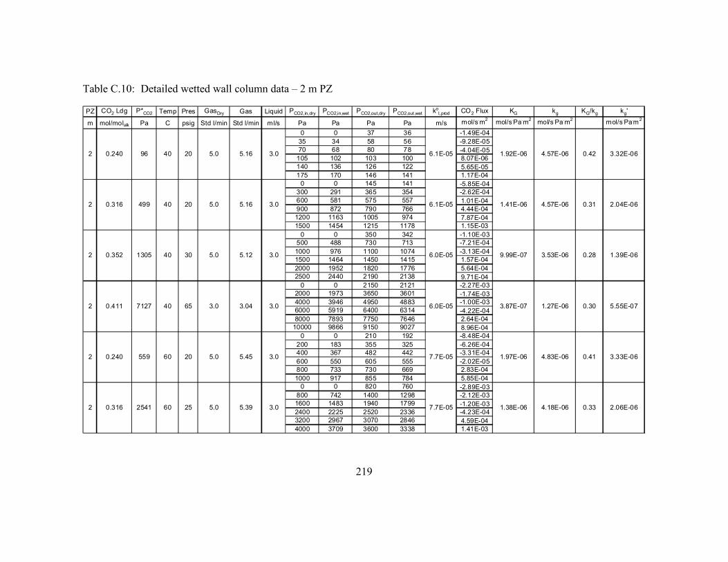
219

Table C.10: Detailed wetted wall column data – 2 m PZ

PZ CO2 Ldg P*CO2 Temp Pres GasDry Gas Liquid PCO2,in,dry PCO2,in,wet PCO2,out,dry PCO2,out,wet kol,prod CO2 Flux KG kg KG/kg kg'


2mol/s

.Pa

.m

2mol/s

.Pa

.m

2mol/s

.Pa

.m

2

0 0 37 36 -1.49E-04

35 34 58 56 -9.28E-05

70 68 80 78 -4.04E-05

105 102 103 100 8.07E-06

140 136 126 122 5.65E-05

175 170 146 141 1.17E-04

0 0 145 141 -5.85E-04

300 291 365 354 -2.62E-04

600 581 575 557 1.01E-04

900 872 790 766 4.44E-04

1200 1163 1005 974 7.87E-04

1500 1454 1215 1178 1.15E-03

0 0 350 342 -1.10E-03

500 488 730 713 -7.21E-04

1000 976 1100 1074 -3.13E-04

1500 1464 1450 1415 1.57E-04

2000 1952 1820 1776 5.64E-04

2500 2440 2190 2138 9.71E-04

0 0 2150 2121 -2.27E-03

2000 1973 3650 3601 -1.74E-03

4000 3946 4950 4883 -1.00E-03

6000 5919 6400 6314 -4.22E-04

8000 7893 7750 7646 2.64E-04

10000 9866 9150 9027 8.96E-04

0 0 210 192 -8.48E-04

200 183 355 325 -6.26E-04

400 367 482 442 -3.31E-04

600 550 605 555 -2.02E-05

800 733 730 669 2.83E-04

1000 917 855 784 5.85E-04

0 0 820 760 -2.89E-03

800 742 1400 1298 -2.12E-03

1600 1483 1940 1799 -1.20E-03

2400 2225 2520 2336 -4.23E-04

3200 2967 3070 2846 4.59E-04

4000 3709 3600 3338 1.41E-03

6.0E-05

6.0E-05

7.7E-05

7.7E-05

6.1E-05

6.1E-05

0.33 2.06E-06

0.41 3.33E-06

0.316 2541 60 25 5.39 3.0 1.38E-06 4.18E-06

0.30 5.55E-07

0.240 559 60 20 5.45 3.0 1.97E-06 4.83E-06

0.28 1.39E-06

0.411 7127 40 65 3.04 3.0 3.87E-07 1.27E-06

0.31 2.04E-06

0.352 1305 40 30 5.12 3.0 9.99E-07 3.53E-06

0.42 3.32E-06

0.316 499 40 20 5.16 3.0 1.41E-06 4.57E-06

0.240 96 40 20 5.16 3.0 1.92E-06 4.57E-06

3.0

5.0

5.0

5.0

5.0

5.0

2

2

2

2

2

2

220




2mol/s

.Pa

.m

2mol/s

.Pa

.m

2mol/s

.Pa

.m

2

0 0 1550 1450 -4.86E-03

3500 3274 4100 3835 -1.88E-03

7000 6547 6800 6360 6.27E-04

10500 9821 9350 8745 3.60E-03

14000 13094 11850 11083 6.74E-03

17500 16368 14550 13609 9.24E-03

0 0 6200 5975 -6.54E-03

10000 9637 13900 13396 -4.11E-03

20000 19274 21400 20624 -1.48E-03

30000 28912 29400 28333 6.33E-04

40000 38549 36700 35368 3.48E-03

50000 48186 44300 42693 6.01E-03

0 0 1050 842 -4.24E-03

1500 1203 2000 1604 -2.02E-03

3000 2406 3050 2446 -2.02E-04

4500 3609 4100 3288 1.61E-03

6000 4812 5000 4010 4.04E-03

7500 6015 6000 4812 6.05E-03

0 0 3750 3279 -9.60E-03

4000 3497 6825 5967 -7.23E-03

8000 6995 9650 8438 -4.22E-03

12000 10492 12600 11017 -1.54E-03

16000 13990 15450 13509 1.41E-03

20000 17487 18325 16023 4.29E-03

0 0 4800 3023 -1.19E-02

5000 3149 8200 5164 -7.90E-03

10000 6297 11900 7494 -4.69E-03

15000 9446 15500 9761 -1.23E-03

20000 12595 18300 11524 4.20E-03

25000 15744 21600 13602 8.40E-03

0 0 14700 11807 -2.20E-02

20000 16064 27800 22330 -1.17E-02

40000 32129 42500 34137 -3.75E-03

60000 48193 56500 45382 5.25E-03

80000 64258 71000 57029 1.35E-02

90000 72290 78500 63053 1.72E-02

1.2E-04

1.3E-04

7.6E-05

7.6E-05

9.9E-05

1.0E-04

0.30 9.12E-07

0.36 2.40E-06

0.324 39286 100 60 4.98 4.1 6.36E-07 2.10E-06

0.29 1.32E-06

0.239 9569 100 25 5.56 3.9 1.55E-06 4.35E-06

0.38 3.34E-06

0.324 12260 80 40 5.72 4.1 9.36E-07 3.21E-06

0.23 3.84E-07

0.239 2492 80 20 6.23 3.9 2.07E-06 5.45E-06

0.27 1.38E-06

0.411 25378 60 65 3.11 3.0 2.97E-07 1.31E-06

0.352 5593 60 30 5.35 3.0 1.00E-06 3.69E-06

3.0

5.0

5.0

5.0

3.5

4.0

2

2

2

2

2

2

221




2mol/s

.Pa

.m

2mol/s

.Pa

.m

2mol/s

.Pa

.m

2

0 0 27 26 -1.09E-04

35 34 49 47 -5.45E-05

70 68 69 66 6.05E-06

105 102 89 86 6.66E-05

140 136 110 106 1.23E-04

175 170 130 126 1.84E-04

0 0 125 121 -5.05E-04

300 291 320 310 -8.07E-05

600 581 510 494 3.63E-04

900 872 715 693 7.47E-04

1200 1163 925 896 1.11E-03

1500 1454 1135 1100 1.47E-03

0 0 345 337 -1.08E-03

500 488 695 678 -6.11E-04

1000 976 1035 1010 -1.10E-04

1500 1464 1405 1371 2.98E-04

2000 1952 1740 1698 8.15E-04

2500 2440 2095 2045 1.27E-03

0 0 1700 1677 -1.79E-03

2000 1973 2925 2886 -9.75E-04

4000 3946 4225 4168 -2.37E-04

6000 5919 5550 5475 4.74E-04

8000 7893 6800 6709 1.27E-03

10000 9866 7975 7868 2.14E-03

0 0 167 153 -6.74E-04

200 183 302 277 -4.12E-04

400 367 412 378 -4.84E-05

600 550 525 481 3.03E-04

800 733 635 582 6.66E-04

1000 917 757 694 9.81E-04

0 0 670 621 -2.36E-03

800 742 1200 1113 -1.41E-03

1600 1483 1730 1604 -4.59E-04

2400 2225 2240 2077 5.64E-04

3200 2967 2790 2587 1.45E-03

4000 3709 3280 3041 2.54E-03

3.6E-05

3.5E-05

4.9E-05

4.8E-05

3.8E-05

3.7E-05

0.39 2.62E-06

0.50 4.75E-06

0.299 1814 60 25 5.39 3.6 1.61E-06 4.18E-06

0.38 7.93E-07

0.226 385 60 20 5.45 3.7 2.40E-06 4.83E-06

0.32 1.69E-06

0.402 4563 40 65 3.04 3.6 4.88E-07 1.27E-06

0.36 2.57E-06

0.354 1120 40 30 5.12 3.6 1.14E-06 3.53E-06

0.49 4.39E-06

0.299 346 40 20 5.16 3.6 1.65E-06 4.57E-06

0.226 65 40 20 5.16 3.7 2.24E-06 4.57E-06

5.0

5.0

5.0

5.0

3.0

5.0

5

5

5

5

5

5

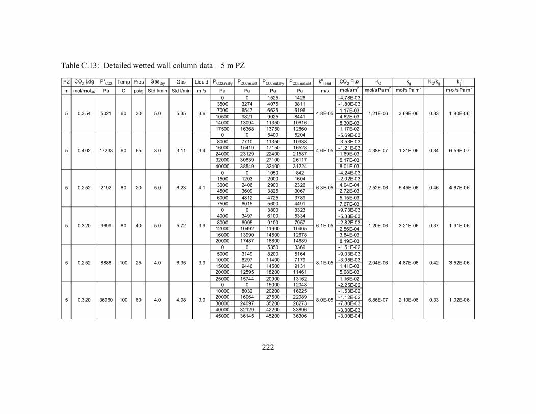
222




2mol/s

.Pa

.m

2mol/s

.Pa

.m

2mol/s

.Pa

.m

2

0 0 1525 1426 -4.78E-03

3500 3274 4075 3811 -1.80E-03

7000 6547 6625 6196 1.17E-03

10500 9821 9025 8441 4.62E-03

14000 13094 11350 10616 8.30E-03

17500 16368 13750 12860 1.17E-02

0 0 5400 5204 -5.69E-03

8000 7710 11350 10938 -3.53E-03

16000 15419 17150 16528 -1.21E-03

24000 23129 22400 21587 1.69E-03

32000 30839 27100 26117 5.17E-03

40000 38549 32400 31224 8.01E-03

0 0 1050 842 -4.24E-03

1500 1203 2000 1604 -2.02E-03

3000 2406 2900 2326 4.04E-04

4500 3609 3825 3067 2.72E-03

6000 4812 4725 3789 5.15E-03

7500 6015 5600 4491 7.67E-03

0 0 3800 3323 -9.73E-03

4000 3497 6100 5334 -5.38E-03

8000 6995 9100 7957 -2.82E-03

12000 10492 11900 10405 2.56E-04

16000 13990 14500 12678 3.84E-03

20000 17487 16800 14689 8.19E-03

0 0 5350 3369 -1.51E-02

5000 3149 8200 5164 -9.03E-03

10000 6297 11400 7179 -3.95E-03

15000 9446 14500 9131 1.41E-03

20000 12595 18200 11461 5.08E-03

25000 15744 20900 13162 1.16E-02

0 0 15000 12048 -2.25E-02

10000 8032 20200 16225 -1.53E-02

20000 16064 27500 22089 -1.12E-02

30000 24097 35200 28273 -7.80E-03

40000 32129 42200 33896 -3.30E-03

45000 36145 45200 36306 -3.00E-04

8.1E-05

8.0E-05

4.8E-05

4.6E-05

6.3E-05

6.1E-05

5

5

5

5

5

5

0.33 1.02E-06

0.42 3.52E-06

0.320 36960 100 60 4.98 3.9 6.86E-07 2.10E-06

0.37 1.91E-06

0.252 8888 100 25 6.35 3.9 2.04E-06 4.87E-06

0.46 4.67E-06

0.320 9699 80 40 5.72 3.9 1.20E-06 3.21E-06

0.34 6.59E-07

0.252 2192 80 20 6.23 4.1 2.52E-06 5.45E-06

0.33 1.80E-06

0.402 17233 60 65 3.11 3.4 4.38E-07 1.31E-06

0.354 5021 60 30 5.35 3.6 1.21E-06 3.69E-06

4.0

3.0

4.0

5.0

5.0

5.0

223




2mol/s

.Pa

.m

2mol/s

.Pa

.m

2mol/s

.Pa

.m

2

0 0 27 26 -1.07E-04

45 44 59 57 -5.45E-05

90 87 83 80 3.03E-05

135 131 109 106 1.05E-04

180 174 134 129 1.88E-04

0 0 165 160 -6.66E-04

300 291 365 354 -2.62E-04

600 581 575 557 1.01E-04

900 872 797 772 4.16E-04

1200 1163 1018 987 7.35E-04

1500 1454 1235 1197 1.07E-03

0 0 465 458 -8.72E-04

500 493 800 789 -5.62E-04

1000 986 1140 1124 -2.62E-04

1500 1478 1465 1444 6.56E-05

2000 1971 1810 1784 3.56E-04

2400 2366 2100 2070 5.62E-04

0 0 2010 1985 -1.99E-03

2000 1975 3625 3579 -1.61E-03

4500 4443 5400 5332 -8.93E-04

7000 6912 7300 7208 -2.98E-04

9500 9380 9225 9108 2.73E-04

11500 11355 10675 10540 8.18E-04

0 0 190 174 -7.67E-04

250 229 340 312 -3.63E-04

500 458 485 445 6.05E-05

750 687 640 587 4.44E-04

1000 917 790 724 8.48E-04

1150 1054 865 793 1.15E-03

0 0 780 723 -2.75E-03

800 742 1320 1224 -1.83E-03

1600 1483 1930 1789 -1.16E-03

2400 2225 2470 2290 -2.47E-04

3200 2967 2990 2772 7.41E-04

4000 3709 3585 3324 1.46E-03

2.1E-05

2.1E-05

3.0E-05

2.8E-05

2.3E-05

2.0E-05

8

8

8

8

8

8

0.33 2.02E-06

0.48 4.41E-06

0.311 2407 60 25 5.39 3.1 1.36E-06 4.18E-06

0.23 3.53E-07

0.235 430 60 20 5.45 3.6 2.31E-06 4.83E-06

0.35 1.14E-06

0.412 8153 40 70 3.04 3.7 2.73E-07 1.19E-06

0.30 1.98E-06

0.340 1409 40 60 5.07 3.7 7.39E-07 2.09E-06

0.48 4.27E-06

0.311 530 40 20 5.16 3.1 1.38E-06 4.57E-06

0.235 68 40 20 5.16 4.0 2.21E-06 4.57E-065.0

5.0

5.0

5.0

3.0

5.0

224




2mol/s

.Pa

.m

2mol/s

.Pa

.m

2mol/s

.Pa

.m

2

0 0 2700 2608 -3.57E-03

2500 2415 4325 4177 -2.41E-03

5000 4829 5975 5771 -1.29E-03

7500 7244 7625 7365 -1.65E-04

10000 9659 9175 8862 1.09E-03

11000 10624 9825 9490 1.55E-03

0 0 7200 6954 -7.14E-03

12000 11590 15800 15261 -3.77E-03

24000 23181 25500 24629 -1.49E-03

36000 34771 35900 34674 9.92E-05

48000 46361 44800 43271 3.17E-03

58000 56020 51700 49935 6.25E-03

0 0 1450 1163 -5.85E-03

1500 1203 2400 1925 -3.63E-03

3000 2406 3275 2626 -1.11E-03

4500 3609 4400 3529 4.04E-04

6000 4812 5350 4290 2.62E-03

7500 6015 6275 5032 4.94E-03

0 0 3600 3148 -9.22E-03

4000 3497 6300 5508 -5.89E-03

8000 6995 8950 7825 -2.43E-03

12000 10492 11700 10230 7.68E-04

16000 13990 14300 12503 4.35E-03

20000 17487 16700 14602 8.45E-03

0 0 7200 4832 -1.58E-02

6000 4027 10700 7181 -1.03E-02

12000 8054 14800 9933 -6.14E-03

18000 12081 18400 12349 -8.77E-04

24000 16108 22900 15369 2.41E-03

30000 20135 26800 17987 7.02E-03

0 0 13800 11084 -2.07E-02

15000 12048 22200 17832 -1.08E-02

30000 24097 33400 26828 -5.10E-03

45000 36145 44400 35663 9.00E-04

60000 48193 53400 42892 9.90E-03

75000 60242 62600 50282 1.86E-02

5.4E-05

5.4E-05

2.9E-05

2.9E-05

4.0E-05

4.0E-05

8

8

8

8

8

8

0.36 1.20E-06

0.37 2.18E-06

0.289 32033 100 60 4.98 4.0 7.63E-07 2.10E-06

0.38 1.97E-06

0.253 13605 100 30 5.21 4.0 1.37E-06 3.66E-06

0.40 3.61E-06

0.289 9406 80 40 5.72 4.0 1.22E-06 3.21E-06

0.21 3.20E-07

0.253 3255 80 20 6.23 4.0 2.17E-06 5.45E-06

0.38 9.57E-07

0.412 30783 60 70 3.11 3.7 2.54E-07 1.23E-06

0.340 7454 60 70 4.14 3.5 5.94E-07 1.57E-06

3.0

4.0

5.0

5.0

3.5

4.0

225




2mol/s

.Pa

.m

2mol/s

.Pa

.m

2mol/s

.Pa

.m

2

0 0 140 128 -5.65E-04

150 137 238 218 -3.55E-04

300 275 327 300 -1.09E-04

450 412 412 378 1.53E-04

600 550 506 464 3.79E-04

750 687 593 544 6.34E-04

0 0 550 510 -1.94E-03

800 742 1150 1066 -1.23E-03

1600 1483 1760 1632 -5.64E-04

2400 2225 2290 2123 3.88E-04

3200 2967 2850 2642 1.23E-03

4000 3709 3420 3171 2.05E-03

0 0 1300 1216 -4.07E-03

3000 2806 3750 3507 -2.35E-03

6000 5612 6100 5705 -3.13E-04

9000 8418 8700 8137 9.40E-04

12000 11224 11300 10569 2.19E-03

15000 14030 13600 12720 4.39E-03

0 0 1025 867 -3.21E-03

1250 1058 1800 1523 -1.72E-03

2500 2116 2550 2158 -1.57E-04

3750 3173 3300 2793 1.41E-03

5000 4231 3925 3322 3.37E-03

6000 5077 4450 3766 4.86E-03

0 0 2900 2536 -7.43E-03

4000 3497 5900 5159 -4.86E-03

8000 6995 8800 7694 -2.05E-03

12000 10492 11800 10317 5.12E-04

16000 13990 14400 12591 4.10E-03

20000 17487 17000 14864 7.68E-03

0 0 4800 3023 -1.19E-02

5000 3149 8200 5164 -7.90E-03

10000 6297 11000 6927 -2.47E-03

15000 9446 14400 9068 1.48E-03

20000 12595 16700 10517 8.15E-03

25000 15744 19900 12532 1.26E-02

1.7E-05

2.4E-05

2.4E-05

3.4E-05

1.8E-05

1.8E-05

12

12

12

12

12

12

0.47 3.78E-06

0.32 1.48E-06

0.222 7871 100 25 5.56 3.9 2.02E-06 4.35E-06

0.51 4.24E-06

0.290 9141 80 40 5.72 3.8 1.01E-06 3.21E-06

0.17 7.73E-07

0.222 2115 80 30 5.91 3.9 2.07E-06 4.04E-06

0.31 1.85E-06

0.354 6791 60 30 5.35 3.8 6.39E-07 3.69E-06

0.46 4.19E-06

0.289 1865 60 25 5.39 3.8 1.28E-06 4.18E-06

0.231 331 60 20 5.45 3.9 2.24E-06 4.83E-06

5.0

3.5

5.0

5.0

5.0

5.0

226




2mol/s

.Pa

.m

2mol/s

.Pa

.m

2mol/s

.Pa

.m

2

0 0 11800 9478 -1.77E-02

15000 12048 21500 17269 -9.75E-03

30000 24097 33400 26828 -5.10E-03

45000 36145 44500 35743 7.50E-04

60000 48193 55500 44579 6.75E-03

75000 60242 65500 52611 1.42E-02

12 3.4E-05 0.28 8.30E-070.290 33652 100 60 4.98 3.9 5.95E-07 2.10E-064.0

227

Table C.18: Detailed wetted wall column data – 7 m MEA/2 m PZ

MEA PZ CO2 Ldg P*CO2 Temp Pres GasDry Gas Liquid PCO2,in,dry PCO2,in,wet PCO2,out,dry PCO2,out,wet kol,prod CO2 Flux KG kg KG/kg kg'

m m mol/molalk Pa C psig Std l/min Std l/min ml/s Pa Pa Pa Pa m/s mol/s.m

2mol/s

.Pa

.m

2mol/s

.Pa

.m

2mol/s

.Pa

.m

2

0 0 9 9 -4.39E-05

10 10 17 17 -3.40E-05

20 19 23 22 -1.18E-05

30 29 29 28 3.30E-06

40 39 36 34 2.12E-05

50 48 43 41 3.54E-05

0 0 52 51 -1.83E-04

100 97 125 122 -8.82E-05

200 195 188 183 4.23E-05

300 292 260 253 1.41E-04

400 389 328 319 2.54E-04

500 487 403 392 3.42E-04

0 0 270 264 -8.46E-04

350 342 580 566 -7.21E-04

700 683 870 849 -5.33E-04

1050 1025 1120 1093 -2.19E-04

1400 1366 1410 1376 -3.13E-05

1750 1708 1690 1650 1.88E-04

0 0 1300 1281 -2.44E-03

4000 3943 4500 4435 -9.37E-04

8000 7885 8001 7886 -1.87E-06

12000 11828 11300 11138 1.31E-03

16000 15771 14550 14341 2.72E-03

20000 19713 17800 17545 4.12E-03

0 0 77 71 -3.11E-04

85 78 129 118 -1.78E-04

170 156 176 161 -2.42E-05

255 234 232 213 9.28E-05

340 312 282 258 2.34E-04

425 390 336 308 3.59E-04

0 0 410 380 -1.45E-03

700 649 905 839 -7.23E-04

1050 974 1140 1057 -3.17E-04

1500 1391 1440 1335 2.12E-04

2000 1854 1810 1678 6.70E-04

2250 2086 1985 1840 9.35E-04

-

-

-

-

-

-

7 2

7 2

7 2

7 2

7 2

7 2

0.33 2.03E-06

0.45 4.00E-06

0.333 1256 60 25 5.39 4.0 1.37E-06 4.18E-06

0.17 4.32E-07

0.242 178 60 20 5.45 4.1 2.19E-06 4.83E-06

0.20 8.76E-07

0.477 7418 40 60 5.07 3.9 3.58E-07 2.09E-06

0.33 1.96E-06

0.416 1425 40 30 5.12 4.0 7.02E-07 3.53E-06

0.39 3.45E-06

0.333 166 40 25 5.14 4.0 1.31E-06 3.98E-06

0.242 27 40 15 5.19 4.0 2.10E-06 5.37E-06

5.0

5.0

5.0

5.0

5.0

5.0

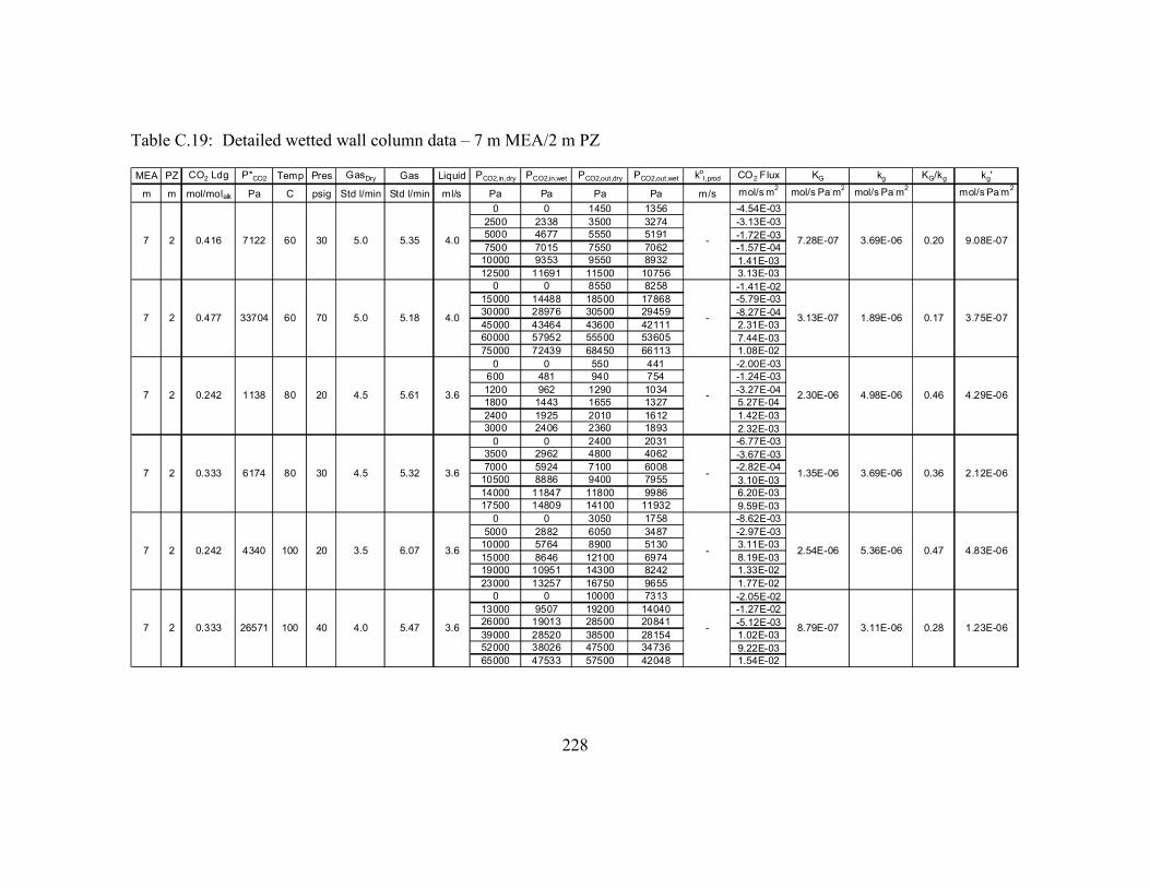
228

Table C.19: Detailed wetted wall column data – 7 m MEA/2 m PZ

MEA PZ CO2 Ldg P*CO2 Temp Pres GasDry Gas Liquid PCO2,in,dry PCO2,in,wet PCO2,out,dry PCO2,out,wet kol,prod CO2 Flux KG kg KG/kg kg'

m m mol/molalk Pa C psig Std l/min Std l/min ml/s Pa Pa Pa Pa m/s mol/s.m

2mol/s

.Pa

.m

2mol/s

.Pa

.m

2mol/s

.Pa

.m

2

0 0 1450 1356 -4.54E-03

2500 2338 3500 3274 -3.13E-03

5000 4677 5550 5191 -1.72E-03

7500 7015 7550 7062 -1.57E-04

10000 9353 9550 8932 1.41E-03

12500 11691 11500 10756 3.13E-03

0 0 8550 8258 -1.41E-02

15000 14488 18500 17868 -5.79E-03

30000 28976 30500 29459 -8.27E-04

45000 43464 43600 42111 2.31E-03

60000 57952 55500 53605 7.44E-03

75000 72439 68450 66113 1.08E-02

0 0 550 441 -2.00E-03

600 481 940 754 -1.24E-03

1200 962 1290 1034 -3.27E-04

1800 1443 1655 1327 5.27E-04

2400 1925 2010 1612 1.42E-03

3000 2406 2360 1893 2.32E-03

0 0 2400 2031 -6.77E-03

3500 2962 4800 4062 -3.67E-03

7000 5924 7100 6008 -2.82E-04

10500 8886 9400 7955 3.10E-03

14000 11847 11800 9986 6.20E-03

17500 14809 14100 11932 9.59E-03

0 0 3050 1758 -8.62E-03

5000 2882 6050 3487 -2.97E-03

10000 5764 8900 5130 3.11E-03

15000 8646 12100 6974 8.19E-03

19000 10951 14300 8242 1.33E-02

23000 13257 16750 9655 1.77E-02

0 0 10000 7313 -2.05E-02

13000 9507 19200 14040 -1.27E-02

26000 19013 28500 20841 -5.12E-03

39000 28520 38500 28154 1.02E-03

52000 38026 47500 34736 9.22E-03

65000 47533 57500 42048 1.54E-02

-

-

-

-

-

-

7 2

7 2

7 2

7 2

7 2

7 2

0.28 1.23E-06

0.47 4.83E-06

0.333 26571 100 40 5.47 3.6 8.79E-07 3.11E-06

0.36 2.12E-06

0.242 4340 100 20 6.07 3.6 2.54E-06 5.36E-06

0.46 4.29E-06

0.333 6174 80 30 5.32 3.6 1.35E-06 3.69E-06

0.17 3.75E-07

0.242 1138 80 20 5.61 3.6 2.30E-06 4.98E-06

0.20 9.08E-07

0.477 33704 60 70 5.18 4.0 3.13E-07 1.89E-06

0.416 7122 60 30 5.35 4.0 7.28E-07 3.69E-06

3.5

4.0

5.0

4.5

4.5

5.0

229

Appendix D: Amine Concentration Effect on CO2 Partial Pressure

This section explains mathematically why CO2 partial pressure should not be a

significant function of amine concentration for carbamate producing systems. Amine

concentration should be important in determining the CO2 partial pressure for bicarbonate

producing systems. The difference is based on the stoichiometry of the reaction.

D.1 CARBAMATE FORMATION

Carbamate forming systems typically have the following stoichiometry:

+− +↔+ AmHAmCOOCOAm 22 (D.1)

The equilibrium constant for this equation can be written as Equation D.2. The

equation can be solved for the partial pressure of CO2 using Equation D.3.

[ ] [ ]

[ ] 2

2

CO

eqPAm

AmHAmCOOK

⋅

⋅=

+−

(D.2)

[ ] [ ]

[ ] eq

COKAm

AmHAmCOOP

⋅

⋅=

+−

22 (D.3)

If only carbamate is being formed, the following assumptions can be made:

[ ] [ ] [ ]TotalAmLdgAmHAmCOO ⋅== +− (D.4)

[ ] ( ) [ ]TotalAmLdgAm ⋅⋅−= 21 (D.5)

Substituting these values into Equation D.3 yields Equation D.6, which does not

have a dependence on the amine concentration of the system.

230

[ ]( ) [ ]( )

( ) [ ]( ) eqeqTotal

TotalTotalCO

KLdg

Ldg

KAmLdg

AmLdgAmLdgP

⋅⋅−=

⋅⋅⋅−

⋅⋅⋅=

2

2

22)21(21

(D.6)

D.2 BICARBONATE FORMATION

Bicarbonate forming systems typically have the following stoichiometry:

+− +↔++ AmHHCOOHCOAm 322 (D.7)

The equilibrium constant for this equation can be written as Equation D.8. The

equation can be solved for the partial pressure of CO2 using Equation D.9.

[ ] [ ][ ] [ ]OHPAm

AmHHCOK

CO

eq

22

3

⋅⋅

⋅=

+−

(D.8)

[ ] [ ][ ] [ ]OHKAm

AmHHCOP

eq

CO

2

3

2 ⋅⋅

⋅=

+−

(D.9)

If only bicarbonate is being formed, the following assumption can be made:

[ ] [ ] [ ]TotalAmLdgAmHHCO ⋅== +−3 (D.10)

[ ] ( ) [ ]TotalAmLdgAm ⋅−= 1 (D.11)

Substituting these values into Equation D.9 yields Equation D.12, which does

have a dependence on the amine concentration of the system.

[ ]( ) [ ]( )

( ) [ ]( ) [ ][ ]

[ ]OHKLdg

AmLdg

OHKAmLdg

AmLdgAmLdgP

eq

Total

eqTotal

TotalTotal

CO

2

2

2

2)1(1 ⋅⋅−

=⋅⋅⋅−

⋅⋅⋅= (D.12)

Equation D.12 shows an expected result. For bicarbonate forming systems the

CO2 partial pressure will increase at constant loading with increases in amine

concentration.

231

Appendix E: Piperazine Density and Viscosity Regressions

E.1 PIPERAZINE DENSITY

Piperazine density data were obtained by regressing 2–12 m PZ density

measurements from Freeman at 20, 40, and 60˚C (Rochelle, Chen et al. 2009a).

The form of the piperazine molar volume equation is shown in Equation E.1,

which uses the weight fractions of CO2 and total PZ. The equation assumes the same

thermal expansion behavior as water. Density can be obtained by dividing the molecular

weight by the molar volume. Table E.1 reports the regressed constants A–D.

+⋅+⋅+⋅= DCBAVV

PZ

CO

PZCOOHPZso ωω

ωω 2

22ln ln (E.1)

ln

lnln

PZso

PZsoPZso

V

MW=ρ (E.2)

Table E.1: Regressed parameters for the PZ molar volume correlation

Parameter Value

A -0.059

B 4.47

C -0.106

D 2.4

Figures E.1–E.4 show the fit of the correlation against the raw data at 2, 5, 8, and

12 m PZ.

232

2 m PZ

0.98

1

1.02

1.04

1.06

1.08

1.1

0 0.1 0.2 0.3 0.4 0.5 0.6


Density (g/cm3)

data 20

data 40

data 60

calc 20

calc 40

calc 60

Figure E.1: 2 m PZ density at 20, 40, and 60˚C: points – data; lines – Equations E.1 and E.2

5 m PZ

1

1.02

1.04

1.06

1.08

1.1

1.12

1.14

1.16

0.0 0.1 0.2 0.3 0.4 0.5 0.6


Density (g/cm3)

data 20

data 40

data 60

calc 20

calc 40

calc 60


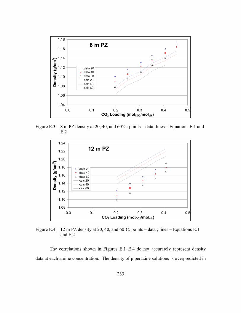
233

8 m PZ

1.04

1.06

1.08

1.10

1.12

1.14

1.16

1.18

0.0 0.1 0.2 0.3 0.4 0.5


Density (g/cm3)

data 20

data 40

data 60

calc 20

calc 40

calc 60


12 m PZ

1.08

1.10

1.12

1.14

1.16

1.18

1.20

1.22

1.24

0.0 0.1 0.2 0.3 0.4 0.5


Density (g/cm3)

data 20

data 40

data 60

calc 20

calc 40

calc 60

Figure E.4: 12 m PZ density at 20, 40, and 60˚C: points – data ; lines – Equations E.1 and E.2

The correlations shown in Figures E.1–E.4 do not accurately represent density

data at each amine concentration. The density of piperazine solutions is overpredicted in

234

2 and 12 m PZ while it is underpredicted in 5 and 8 m PZ. The correlation averaged

1.5% error over the total data range: 2, 5, 7, 8, 9, 10, and 12 m PZ solutions.

Solution density is not an important parameter in these analyses. Density is

required to calculate the liquid film mass transfer coefficient of the reactants and

products. In many cases this term is negligible. When diffusion resistances become

significant, density has a 1/6th order dependence on o

prodlk

, (Equation 3.16). Unlike

viscosity, solution densities do not vary more than 20% over the total range of

experimental conditions.

E.2 PIPERAZINE VISCOSITY

PZ solution viscosity values were obtained by regressing 5–12 m PZ viscosity

measurements from Freeman at 25, 40, and 60˚C (Rochelle, Sexton et al. 2008a).

The form of the piperazine viscosity equation was based on the form Weiland

(1998) used for MEA viscosity. Equation E.3 is linked to the viscosity of water and

utilizes the wt% of piperazine on a CO2-free basis. Temperatures are in Kelvin and

loading is in molCO2/molalk. Table E.2 includes the regressed parameters. Figures E.5–

E.7 show the fit of Equation E.3 to experimental data.

( ) ( )[ ] ( )[ ]

Ω+++Ω⋅+Ω++Ω=

22

1exp

T

gfTedcTbaOH

αηη (E.3)

Table E.2: Regressed parameters for the PZ viscosity equation

Parameter a b c d e f g

Value 0.310 5.71 0.417 0.0267 -0.00752 -0.00574 2.51

235

PZ, 25C

1

10

100

0.2 0.25 0.3 0.35 0.4 0.45 0.5


Viscosity (cP)

5 m PZ 7 m PZ 9 m PZ 10 m PZ 12 m PZ

Figure E.5: 5–12 m PZ viscosity at 25˚C: points – data; lines – Equation E.3

PZ, 40C

1

10

100

0.2 0.25 0.3 0.35 0.4 0.45 0.5


Viscosity (cP)



236

PZ, 60C

1

10

100

0.2 0.25 0.3 0.35 0.4 0.45 0.5


Viscosity (cP)



Figures E.5–E.7 show good agreement between the viscosity correlation and the

raw data. Viscosity was properly represented over the 5–12 m PZ, 25–60˚C range. Parts

of the model required the extrapolation of Equation E.3 to 2 m PZ and up to 100˚C. The

satisfactory fit with respect to changing temperature and PZ concentration in Figures

E.5–E.7 suggests that the extrapolation to 2 m or 100˚C will not introduce significant

error.

Unlike density, viscosity estimation is very important for amine solutions.

Piperazine solution viscosities can change a factor of 10 with changes in amine

concentration. These viscosity changes can drastically affect o

prodlk

,as well as the diffusion

coefficient of CO2.

237

Appendix F: Calculated Spreadsheet Model Values

This section lists calculated values for the MEA and PZ spreadsheet models.

Each parameter in the kg’ expressions is included in the following tables. Most of these

data were generated to produce the figures presented in Chapter 5.

238

Table F.1: Calculated spreadsheet model results for 7 and 9 m MEA wetted wall column conditions

MEA Temp CO2 Loading [MEA]free γCO2 γMEA HCO2,soln Density Viscosity DCO2 d(PCO2)d(ldg) [Alk] Slope Equil kol,prod kl

o/slope kg'' Diffusion Calc kg' Exp kg'

m C molCO2/molalk M Pa.m

3/mol g/cm

3cP m

2/s Pa/(mol/molalk) molalk/m

3 Pa/(mol/m3) m/s mol/s

.Pa

.m

2mol/s

.Pa

.m

2Resistance mol/s

.Pa

.m

2mol/s

.Pa

.m

2

0.252 2.45 1.53 0.62 6317 1.06 2.00 1.2E-09 215 4916 0.04 4.61E-05 1.05E-03 2.90E-06 0% 2.89E-06 3.34E-06

0.351 1.49 1.74 0.74 7199 1.08 2.18 1.1E-09 1516 4916 0.31 4.40E-05 1.43E-04 1.90E-06 1% 1.88E-06 1.40E-06

0.432 0.72 1.94 0.85 8011 1.10 2.34 1.1E-09 9414 4916 1.92 4.23E-05 2.21E-05 9.82E-07 4% 9.40E-07 7.66E-07

0.496 0.21 2.11 0.95 8717 1.11 2.48 1.0E-09 46265 4915 9.41 4.11E-05 4.36E-06 3.02E-07 6% 2.82E-07 3.47E-07

0.252 2.42 1.42 0.47 8692 1.04 1.31 1.9E-09 1534 4849 0.32 5.94E-05 1.88E-04 3.20E-06 2% 3.14E-06 2.92E-06

0.351 1.48 1.62 0.56 9906 1.06 1.43 1.8E-09 8925 4849 1.84 5.65E-05 3.07E-05 2.11E-06 6% 1.97E-06 1.70E-06

0.432 0.74 1.81 0.64 11023 1.08 1.54 1.7E-09 47050 4848 9.70 5.43E-05 5.60E-06 1.12E-06 17% 9.32E-07 9.28E-07

0.496 0.26 1.96 0.71 11995 1.09 1.64 1.6E-09 202553 4848 41.78 5.26E-05 1.26E-06 4.09E-07 25% 3.09E-07 3.76E-07

0.271 2.21 1.37 0.37 11829 1.03 0.99 2.8E-09 11415 4787 2.38 6.73E-05 2.82E-05 3.20E-06 10% 2.87E-06 2.85E-06

0.366 1.33 1.55 0.44 13409 1.05 1.08 2.6E-09 55364 4787 11.57 6.41E-05 5.55E-06 2.06E-06 27% 1.50E-06 1.87E-06

0.271 2.18 1.29 0.30 15229 1.02 0.64 4.4E-09 50599 4719 10.72 8.65E-05 8.07E-06 3.60E-06 31% 2.49E-06 2.98E-06

0.366 1.32 1.46 0.35 17264 1.04 0.71 4.1E-09 214665 4719 45.49 8.24E-05 1.81E-06 2.33E-06 56% 1.02E-06 1.40E-06

0.231 3.14 1.62 0.60 6674 1.06 2.58 1.0E-09 148 5831 0.03 4.03E-05 1.59E-03 3.19E-06 0% 3.19E-06 -

0.324 2.07 1.87 0.71 7724 1.09 2.87 9.3E-10 863 5831 0.15 3.81E-05 2.57E-04 2.21E-06 1% 2.19E-06 1.86E-06

0.382 1.41 2.05 0.78 8461 1.10 3.06 8.9E-10 2975 5830 0.51 3.67E-05 7.20E-05 1.55E-06 2% 1.52E-06 1.40E-06

0.441 0.74 2.25 0.87 9283 1.12 3.28 8.5E-10 11683 5830 2.00 3.54E-05 1.77E-05 8.44E-07 5% 8.06E-07 8.36E-07

0.496 0.22 2.45 0.95 10121 1.13 3.49 8.1E-10 46265 5829 7.94 3.43E-05 4.32E-06 2.53E-07 6% 2.39E-07 3.02E-07

0.231 3.10 1.50 0.45 9184 1.05 1.64 1.6E-09 1096 5751 0.19 5.26E-05 2.76E-04 3.55E-06 1% 3.50E-06 3.80E-06

0.324 2.05 1.74 0.53 10629 1.07 1.83 1.5E-09 5364 5750 0.93 4.96E-05 5.31E-05 2.46E-06 4% 2.35E-06 2.44E-06

0.382 1.40 1.91 0.59 11643 1.09 1.97 1.4E-09 16461 5749 2.86 4.78E-05 1.67E-05 1.74E-06 9% 1.57E-06 1.47E-06

0.441 0.77 2.09 0.65 12774 1.10 2.11 1.4E-09 57318 5749 9.97 4.60E-05 4.62E-06 9.78E-07 17% 8.07E-07 9.57E-07

0.496 0.28 2.28 0.71 13926 1.12 2.25 1.3E-09 202553 5749 35.23 4.44E-05 1.26E-06 3.62E-07 22% 2.81E-07 3.24E-07

0.265 2.68 1.49 0.37 12857 1.04 1.24 2.4E-09 10420 5675 1.84 6.25E-05 3.41E-05 3.39E-06 9% 3.08E-06 3.24E-06

0.356 1.68 1.72 0.43 14833 1.07 1.39 2.2E-09 46313 5675 8.16 6.39E-05 7.82E-06 2.22E-06 22% 1.73E-06 1.75E-06

0.265 2.64 1.40 0.29 16554 1.03 0.80 3.8E-09 46549 5593 8.32 7.93E-05 9.52E-06 3.84E-06 29% 2.74E-06 3.40E-06

0.356 1.66 1.62 0.35 19098 1.05 0.89 3.5E-09 182248 5592 32.59 8.12E-05 2.49E-06 2.52E-06 50% 1.25E-06 1.33E-06100

7

9

40

60

80

100

40

60

80

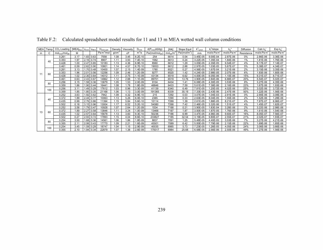
239

Table F.2: Calculated spreadsheet model results for 11 and 13 m MEA wetted wall column conditions




3/mol g/cm

3cP m



.Pa

.m

2mol/s

.Pa

.m

2Resistance mol/s

.Pa

.m

2mol/s

.Pa

.m

2

0.261 3.17 1.83 0.63 7558 1.08 3.45 8.2E-10 254 6614 0.04 3.45E-05 9.00E-04 2.87E-06 0% 2.86E-06 3.36E-06

0.353 1.97 2.16 0.74 8907 1.11 3.93 7.4E-10 1582 6613 0.24 3.22E-05 1.35E-04 1.84E-06 1% 1.81E-06 1.76E-06

0.428 1.00 2.47 0.85 10183 1.13 4.36 6.9E-10 8560 6612 1.29 3.05E-05 2.35E-05 9.54E-07 4% 9.17E-07 7.14E-07

0.461 0.59 2.62 0.90 10801 1.14 4.57 6.7E-10 19053 6612 2.88 2.97E-05 1.03E-05 5.67E-07 5% 5.38E-07 4.34E-07

0.261 3.13 1.70 0.48 10400 1.07 2.15 1.4E-09 1780 6521 0.27 4.56E-05 1.67E-04 3.21E-06 2% 3.15E-06 3.35E-06

0.353 1.96 2.01 0.56 12256 1.09 2.46 1.2E-09 9277 6520 1.42 4.24E-05 2.98E-05 2.07E-06 6% 1.93E-06 1.80E-06

0.428 1.02 2.30 0.64 14012 1.11 2.75 1.1E-09 43134 6519 6.62 4.00E-05 6.05E-06 1.10E-06 15% 9.31E-07 8.71E-07

0.461 0.63 2.43 0.67 14862 1.12 2.88 1.1E-09 89701 6519 13.76 3.90E-05 2.84E-06 6.88E-07 20% 5.54E-07 5.02E-07

0.256 3.15 1.58 0.36 13679 1.05 1.53 2.0E-09 9104 6434 1.41 6.08E-05 4.30E-05 3.53E-06 8% 3.27E-06 4.35E-06

0.359 1.86 1.90 0.44 16441 1.08 1.78 1.8E-09 48846 6433 7.59 5.61E-05 7.38E-06 2.16E-06 23% 1.67E-06 1.93E-06

0.256 3.11 1.49 0.29 17612 1.03 0.96 3.3E-09 41139 6340 6.49 7.81E-05 1.20E-05 4.02E-06 25% 3.02E-06 3.72E-06

0.359 1.85 1.80 0.35 21168 1.06 1.13 3.0E-09 191365 6339 30.19 7.33E-05 2.43E-06 2.47E-06 50% 1.22E-06 1.56E-06

0.252 3.63 1.92 0.62 7942 1.09 4.32 6.9E-10 215 7292 0.03 3.07E-05 1.04E-03 2.91E-06 0% 2.90E-06 3.08E-06

0.372 1.89 2.44 0.77 10063 1.13 5.26 6.0E-10 2385 7290 0.33 2.63E-05 8.04E-05 1.55E-06 2% 1.52E-06 1.28E-06

0.435 0.99 2.76 0.86 11394 1.15 5.84 5.6E-10 10114 7289 1.39 2.61E-05 1.88E-05 8.21E-07 4% 7.87E-07 6.96E-07

0.502 0.18 3.15 0.96 13004 1.17 6.52 5.2E-10 54080 7288 7.42 2.46E-05 3.32E-06 1.51E-07 4% 1.45E-07 1.62E-07

0.252 3.58 1.79 0.47 10928 1.07 2.64 1.2E-09 1534 7188 0.21 3.90E-05 1.83E-04 3.28E-06 2% 3.22E-06 2.98E-06

0.372 1.89 2.27 0.58 13846 1.11 3.24 1.0E-09 13468 7187 1.87 3.50E-05 1.87E-05 1.76E-06 9% 1.61E-06 1.54E-06

0.435 1.02 2.57 0.64 15678 1.13 3.60 9.3E-10 50236 7186 6.99 3.47E-05 4.96E-06 9.60E-07 16% 8.05E-07 7.56E-07

0.502 0.27 2.93 0.72 17893 1.15 4.04 8.6E-10 233827 7185 32.54 3.19E-05 9.80E-07 2.55E-07 21% 2.02E-07 1.93E-07

0.254 3.50 1.68 0.36 14561 1.06 1.86 1.8E-09 8837 7091 1.25 5.48E-05 4.40E-05 3.53E-06 7% 3.27E-06 4.21E-06

0.355 2.11 2.06 0.43 17770 1.09 2.21 1.6E-09 45501 7089 6.42 5.00E-05 7.79E-06 2.15E-06 22% 1.69E-06 1.85E-06

0.254 3.45 1.59 0.29 18747 1.04 1.15 2.9E-09 40035 6985 5.73 7.23E-05 1.26E-05 4.05E-06 24% 3.06E-06 3.66E-06

0.355 2.10 1.94 0.34 22879 1.07 1.38 2.6E-09 179317 6984 25.68 6.58E-05 2.56E-06 2.50E-06 49% 1.27E-06 1.56E-06100

11

13

40

60

80

100

40

60

80

240

Table F.3: Calculated spreadsheet model results for 7 and 13 m MEA at 20˚C (Figure 5.45)

MEA Temp CO2 Loading [MEA]free γCO2 γMEA HCO2,soln Density Viscosity DCO2 d(PCO2)d(ldg) [Alk] Slope Equil kol,prod klo/slope kg'' Diffusion Calc kg'


3/mol g/cm

3cP m



.Pa

.m

2mol/s

.Pa

.m

2Resistance mol/s

.Pa

.m

2

0.25 2.48 1.66 0.86 4383 1.07 3.57 6.8E-10 22 4960 0.00 3.28E-05 7.54E-03 2.55E-06 0% 2.55E-06

0.3 1.99 1.77 0.94 4682 1.08 3.72 6.6E-10 62 4960 0.01 3.21E-05 2.56E-03 2.12E-06 0% 2.12E-06

0.35 1.50 1.89 1.03 5002 1.09 3.88 6.4E-10 194 4960 0.04 3.15E-05 8.03E-04 1.66E-06 0% 1.66E-06

0.4 1.01 2.02 1.12 5343 1.10 4.04 6.3E-10 657 4960 0.13 3.08E-05 2.32E-04 1.17E-06 0% 1.16E-06

0.45 0.53 2.16 1.22 5708 1.11 4.20 6.1E-10 2408 4960 0.49 3.01E-05 6.20E-05 6.41E-07 1% 6.34E-07

0.5 0.14 2.31 1.33 6097 1.12 4.38 5.9E-10 9581 4959 1.93 2.95E-05 1.53E-05 1.74E-07 1% 1.72E-07

0.55 0.03 2.46 1.45 6513 1.13 4.56 5.7E-10 41401 4959 8.35 2.89E-05 3.46E-06 3.69E-08 1% 3.65E-08

0.6 0.01 2.63 1.59 6958 1.14 4.74 5.6E-10 194358 4959 39.19 2.82E-05 7.20E-07 1.53E-08 2% 1.50E-08

0.25 3.69 2.08 0.86 5504 1.10 8.33 3.7E-10 22 7367 0.00 2.28E-05 7.76E-03 2.49E-06 0% 2.49E-06

0.3 2.95 2.30 0.94 6074 1.11 9.01 3.5E-10 62 7366 0.01 2.18E-05 2.58E-03 2.01E-06 0% 2.01E-06

0.35 2.22 2.54 1.03 6704 1.13 9.74 3.3E-10 194 7366 0.03 2.06E-05 7.80E-04 1.53E-06 0% 1.52E-06

0.4 1.49 2.80 1.12 7399 1.15 10.53 3.1E-10 657 7365 0.09 2.01E-05 2.25E-04 1.03E-06 0% 1.03E-06

0.45 0.76 3.09 1.22 8166 1.16 11.39 3.0E-10 2408 7364 0.33 1.78E-05 5.44E-05 5.33E-07 1% 5.27E-07

0.5 0.12 3.41 1.33 9012 1.18 12.32 2.8E-10 9581 7364 1.30 1.63E-05 1.25E-05 8.71E-08 1% 8.65E-08

0.55 0.02 3.76 1.45 9946 1.19 13.32 2.6E-10 41401 7363 5.62 1.64E-05 2.91E-06 1.22E-08 0% 1.22E-08

0.6 0.01 4.15 1.59 10977 1.21 14.40 2.5E-10 194358 7362 26.40 1.57E-05 5.95E-07 5.62E-09 1% 5.57E-09

20

7

13

Table F.4: Calculated spreadsheet model results for 9 m MEA at 0.3 CO2 loading (Figure 5.18)


o/slope kg'' Diffusion Calc kg'


3/mol g/cm

3cP m



.Pa

.m

2mol/s

.Pa

.m

2Resistance mol/s

.Pa

.m

2

40 2.35 1.80 0.68 7439 1.08 2.79 9.3E-10 534 5831 0.09 3.86E-05 4.22E-04 2.45E-06 1% 2.44E-06

50 2.34 1.74 0.58 8769 1.07 2.18 1.2E-09 1405 5798 0.24 4.46E-05 1.84E-04 2.60E-06 1% 2.56E-06

60 2.32 1.68 0.51 10236 1.07 1.78 1.5E-09 3475 5750 0.60 5.03E-05 8.33E-05 2.73E-06 3% 2.64E-06

70 2.31 1.62 0.45 11840 1.06 1.51 1.9E-09 8117 5713 1.42 5.57E-05 3.92E-05 2.86E-06 7% 2.67E-06

80 2.29 1.57 0.39 13584 1.05 1.30 2.4E-09 17989 5675 3.17 6.11E-05 1.93E-05 2.99E-06 13% 2.59E-06

90 2.28 1.53 0.35 15467 1.04 1.09 2.9E-09 37984 5635 6.74 6.80E-05 1.01E-05 3.12E-06 24% 2.38E-06

100 2.26 1.48 0.31 17489 1.04 0.83 3.5E-09 76688 5593 13.71 7.93E-05 5.78E-06 3.24E-06 36% 2.07E-06

9 0.3

241

Table F.5: Calculated MEA spreadsheet model results for 60˚C, 0.4 CO2 loading MEA solutions (Figure 5.19)




3/mol g/cm

3cP m



.Pa

.m

2mol/s

.Pa

.m

2Resistance mol/s

.Pa

.m

2

7 1.03 1.73 0.61 10567 1.07 1.50 1.7E-09 23809 4849 4.91 5.52E-05 1.12E-05 1.50E-06 12% 1.33E-06

8 1.12 1.84 0.61 11263 1.08 1.73 1.6E-09 23809 5316 4.48 4.86E-05 1.09E-05 1.51E-06 12% 1.32E-06

9 1.21 1.96 0.61 11977 1.09 2.01 1.4E-09 23809 5749 4.14 4.50E-05 1.09E-05 1.49E-06 12% 1.31E-06

10 1.29 2.07 0.61 12649 1.10 2.30 1.3E-09 23809 6148 3.87 4.19E-05 1.08E-05 1.48E-06 12% 1.30E-06

11 1.36 2.18 0.61 13329 1.11 2.64 1.2E-09 23809 6520 3.65 3.90E-05 1.07E-05 1.45E-06 12% 1.28E-06

12 1.43 2.29 0.61 13981 1.11 3.00 1.0E-09 23809 6864 3.47 3.83E-05 1.10E-05 1.42E-06 11% 1.26E-06

13 1.50 2.40 0.61 14633 1.12 3.40 9.6E-10 23809 7186 3.31 3.58E-05 1.08E-05 1.39E-06 11% 1.23E-06

60 0.4

Table F.6: Calculated spreadsheet model results for 7 and 9 m MEA at high CO2 loading and temperature




3/mol g/cm

3cP m



.Pa

.m

2mol/s

.Pa

.m

2Resistance mol/s

.Pa

.m

2

80 0.59 1.73 0.51 14963 1.07 1.17 2.5E-09 279459 4786 58.39 6.46E-05 1.11E-06 9.74E-07 47% 5.18E-07

100 0.67 1.63 0.41 19265 1.06 0.77 3.9E-09 952786 4718 201.95 8.29E-05 4.10E-07 1.25E-06 75% 3.09E-07

80 0.90 2.48 0.51 21411 1.12 2.61 1.4E-09 279459 7087 39.43 4.23E-05 1.07E-06 9.28E-07 46% 4.98E-07

100 0.92 2.34 0.41 27566 1.10 1.62 2.3E-09 952786 6982 136.47 5.57E-05 4.08E-07 1.11E-06 73% 2.98E-07

0.45

7

13

Table F.7: Calculated spreadsheet model results for Hartono (2009) experimental conditions (Figure 5.43)

MEA Temp CO2 Loading [MEA]free γCO2 γMEA HCO2,soln Density Viscosity DCO2 kg'' Exp kg'

M C molCO2/molalk M Pa.m

3/mol g/cm

3cP m

2/s mol/s

.Pa

.m

2mol/s

.Pa

.m

2

0.5 40 0 0.5 0.972 0.326 4010 0.99 0.69 2.6E-09 5.71E-07 1.07E-06

1 40 0 1.0 0.985 0.326 4065 0.99 0.74 2.5E-09 1.10E-06 1.72E-06

2 40 0 2.0 1.013 0.326 4181 1.00 0.89 2.2E-09 2.04E-06 2.24E-06

3 40 0 3.0 1.041 0.326 4296 1.00 1.07 1.9E-09 2.83E-06 2.61E-06

4 40 0 4.0 1.070 0.326 4416 1.00 1.31 1.6E-09 3.45E-06 2.80E-06

5 40 0 5.0 1.100 0.326 4539 1.00 1.60 1.4E-09 3.96E-06 2.88E-06

242

Table F.8: Calculated pseudo first order spreadsheet model results for 5 M MEA at 40 and 60˚C (Figure 5.42)

MEA Temp CO2 Loading [MEA]free γCO2 γMEA HCO2,soln Density Viscosity DCO2 kg''


3/mol g/cm

3cP m

2/s mol/s

.Pa

.m

2

0 4.92 1.10 0.40 4529 1.00 1.60 1.4E-09 4.77E-06

0.05 4.43 1.17 0.44 4838 1.01 1.67 1.4E-09 4.46E-06

0.1 3.93 1.25 0.48 5168 1.02 1.75 1.3E-09 4.12E-06

0.15 3.44 1.34 0.52 5521 1.04 1.83 1.3E-09 3.74E-06

0.2 2.95 1.43 0.57 5898 1.05 1.91 1.2E-09 3.34E-06

0.25 2.47 1.53 0.62 6300 1.06 2.00 1.2E-09 2.89E-06

0.3 1.98 1.63 0.68 6730 1.07 2.08 1.2E-09 2.41E-06

0.35 1.50 1.74 0.74 7189 1.08 2.18 1.1E-09 1.90E-06

0.4 1.02 1.86 0.81 7680 1.09 2.28 1.1E-09 1.34E-06

0.45 0.56 1.99 0.88 8204 1.10 2.38 1.0E-09 7.65E-07

0.5 0.19 2.12 0.96 8764 1.11 2.49 1.0E-09 2.69E-07

0 4.85 1.02 0.30 6232 0.99 1.03 2.3E-09 5.28E-06

0.05 4.37 1.09 0.33 6657 1.00 1.08 2.2E-09 4.93E-06

0.1 3.88 1.16 0.36 7112 1.01 1.13 2.1E-09 4.55E-06

0.15 3.40 1.24 0.39 7597 1.02 1.19 2.0E-09 4.14E-06

0.2 2.92 1.33 0.43 8115 1.03 1.24 2.0E-09 3.68E-06

0.25 2.44 1.42 0.47 8669 1.04 1.30 1.9E-09 3.20E-06

0.3 1.96 1.52 0.51 9261 1.05 1.36 1.8E-09 2.67E-06

0.35 1.49 1.62 0.55 9892 1.06 1.43 1.8E-09 2.10E-06

0.4 1.03 1.73 0.61 10567 1.07 1.50 1.7E-09 1.50E-06

0.45 0.59 1.85 0.66 11289 1.08 1.57 1.7E-09 8.92E-07

0.5 0.24 1.98 0.72 12059 1.10 1.64 1.6E-09 3.74E-07

5

40

60

243

Table F.9: Calculated pseudo first order spreadsheet model results for 7 M MEA at 40 and 60˚C (Figure 5.42)

MEA Temp CO2 Loading [MEA]free γCO2 γMEA HCO2,soln Density Viscosity DCO2 kg''


3/mol g/cm

3cP m

2/s mol/s

.Pa

.m

2

0 6.97 1.16 0.40 4786 1.01 2.60 9.8E-10 5.52E-06

0.05 6.27 1.27 0.44 5257 1.02 2.81 9.3E-10 5.03E-06

0.1 5.57 1.40 0.48 5774 1.04 3.03 8.8E-10 4.53E-06

0.15 4.88 1.54 0.52 6342 1.05 3.27 8.3E-10 4.01E-06

0.2 4.18 1.69 0.57 6965 1.07 3.53 7.9E-10 3.49E-06

0.25 3.49 1.85 0.62 7651 1.08 3.81 7.5E-10 2.95E-06

0.3 2.80 2.04 0.68 8403 1.10 4.11 7.1E-10 2.39E-06

0.35 2.11 2.24 0.74 9230 1.11 4.43 6.7E-10 1.83E-06

0.4 1.43 2.46 0.81 10138 1.13 4.78 6.3E-10 1.25E-06

0.45 0.75 2.70 0.88 11135 1.14 5.16 6.0E-10 6.69E-07

0.5 0.19 2.96 0.96 12230 1.16 5.57 5.7E-10 1.74E-07

0 6.87 1.08 0.30 6585 0.99 1.59 1.7E-09 6.23E-06

0.05 6.18 1.18 0.33 7233 1.01 1.72 1.6E-09 5.67E-06

0.1 5.50 1.30 0.36 7945 1.02 1.86 1.5E-09 5.10E-06

0.15 4.81 1.43 0.39 8726 1.04 2.01 1.4E-09 4.52E-06

0.2 4.13 1.57 0.43 9585 1.05 2.17 1.3E-09 3.92E-06

0.25 3.45 1.72 0.47 10527 1.07 2.35 1.2E-09 3.32E-06

0.3 2.77 1.89 0.51 11563 1.08 2.54 1.2E-09 2.70E-06

0.35 2.10 2.08 0.55 12700 1.10 2.75 1.1E-09 2.07E-06

0.4 1.43 2.28 0.61 13950 1.11 2.98 1.1E-09 1.43E-06

0.45 0.79 2.51 0.66 15322 1.13 3.22 1.0E-09 7.97E-07

0.5 0.27 2.76 0.72 16829 1.14 3.49 9.4E-10 2.80E-07

7

40

60

244

Table F.10: Calculated spreadsheet model results for 2, 5, 8, and 12 m PZ wetted wall column conditions

PZ Temp CO2 Loading [PZ]free [PZCOO-] γCO2 γPZ γPZCOO HCO2,soln Density Viscosity DCO2 d(PCO2)d(ldg) [Alk] Slope Equil k

ol,prod kl


m C molCO2/molalk M M Pa.m

3/mol g/cm

3cP m



.Pa

.m

2mol/s

.Pa

.m

2Resistance mol/s

.Pa

.m

2mol/s

.Pa

.m

2

0.24 0.48 0.32 1.38 0.057 0.038 5698 1.04 1.11 1.9E-09 2255 3421 0.66 6.14E-05 9.32E-05 3.38E-06 4% 3.26E-06 3.32E-06

0.316 0.21 0.32 1.52 0.057 0.038 6264 1.05 1.13 1.8E-09 13581 3419 3.97 6.07E-05 1.53E-05 1.87E-06 11% 1.67E-06 2.04E-06

0.352 0.13 0.27 1.59 0.057 0.038 6551 1.05 1.14 1.8E-09 32203 3419 9.42 6.04E-05 6.41E-06 1.32E-06 17% 1.09E-06 1.39E-06

0.411 0.05 0.15 1.71 0.057 0.038 7050 1.06 1.16 1.8E-09 134954 3418 39.49 5.98E-05 1.51E-06 5.96E-07 28% 4.28E-07 5.55E-07

0.24 0.55 0.22 1.28 0.080 0.038 7841 1.03 0.76 2.9E-09 11494 3390 3.39 7.72E-05 2.28E-05 5.88E-06 21% 4.67E-06 3.33E-06

0.316 0.28 0.21 1.41 0.080 0.038 8619 1.04 0.77 2.8E-09 57257 3388 16.90 7.65E-05 4.53E-06 3.16E-06 41% 1.86E-06 2.06E-06

0.352 0.19 0.17 1.48 0.080 0.038 9014 1.05 0.78 2.8E-09 124088 3388 36.63 7.62E-05 2.08E-06 2.17E-06 51% 1.06E-06 1.38E-06

0.411 0.08 0.10 1.59 0.080 0.038 9701 1.05 0.79 2.8E-09 448729 3387 132.50 7.56E-05 5.71E-07 9.57E-07 63% 3.58E-07 3.84E-07

0.239 0.58 0.14 1.20 0.106 0.038 10393 1.02 0.59 4.0E-09 47213 3350 14.09 9.90E-05 7.02E-06 9.58E-06 58% 4.05E-06 3.34E-06

0.324 0.29 0.13 1.34 0.106 0.038 11553 1.03 0.60 4.0E-09 236248 3349 70.54 1.00E-04 1.42E-06 4.72E-06 77% 1.09E-06 1.32E-06

0.239 0.59 0.09 1.14 0.138 0.038 13381 1.00 0.40 6.3E-09 167679 3304 50.75 1.25E-04 2.46E-06 1.57E-05 86% 2.13E-06 2.40E-06

0.324 0.30 0.08 1.26 0.138 0.038 14875 1.01 0.40 6.2E-09 710204 3303 215.04 1.27E-04 5.89E-07 7.74E-06 93% 5.47E-07 9.12E-07

0.226 0.84 0.95 2.00 0.075 0.038 8246 1.04 3.19 8.6E-10 1627 6801 0.24 3.76E-05 1.57E-04 4.70E-06 3% 4.56E-06 4.39E-06

0.299 0.30 0.95 2.43 0.075 0.038 10006 1.06 3.36 8.3E-10 9060 6774 1.34 3.66E-05 2.74E-05 2.39E-06 8% 2.20E-06 2.57E-06

0.354 0.15 0.71 2.81 0.075 0.038 11576 1.07 3.49 8.1E-10 33794 6753 5.00 3.58E-05 7.16E-06 1.39E-06 16% 1.16E-06 1.69E-06

0.402 0.08 0.45 3.19 0.075 0.038 13145 1.08 3.61 7.9E-10 108302 6735 16.08 3.52E-05 2.19E-06 7.74E-07 26% 5.72E-07 7.93E-07

0.226 0.98 0.72 1.86 0.104 0.038 11347 1.03 2.00 1.4E-09 8585 6739 1.27 4.95E-05 3.88E-05 8.47E-06 18% 6.96E-06 4.75E-06

0.299 0.47 0.69 2.26 0.104 0.038 13768 1.05 2.08 1.4E-09 39852 6712 5.94 4.85E-05 8.17E-06 4.31E-06 35% 2.82E-06 2.62E-06

0.354 0.26 0.51 2.61 0.104 0.038 15928 1.06 2.14 1.4E-09 129567 6692 19.36 4.78E-05 2.47E-06 2.42E-06 49% 1.22E-06 1.80E-06

0.402 0.14 0.32 2.96 0.104 0.038 18088 1.07 2.19 1.3E-09 368302 6674 55.18 4.62E-05 8.37E-07 1.29E-06 61% 5.08E-07 6.59E-07

0.238 0.99 0.52 1.80 0.139 0.038 15546 1.02 1.44 2.1E-09 46339 6657 6.96 6.28E-05 9.02E-06 1.31E-05 59% 5.34E-06 4.67E-06

0.321 0.48 0.44 2.24 0.139 0.038 19369 1.04 1.48 2.1E-09 223023 6626 33.66 6.08E-05 1.81E-06 6.12E-06 77% 1.39E-06 1.91E-06

0.238 1.04 0.36 1.70 0.179 0.038 20015 1.01 0.91 3.5E-09 164900 6565 25.12 8.08E-05 3.22E-06 2.24E-05 87% 2.81E-06 3.52E-06

0.321 0.52 0.31 2.12 0.179 0.038 24938 1.03 0.92 3.4E-09 674404 6535 103.20 8.02E-05 7.77E-07 1.03E-05 93% 7.22E-07 1.02E-06

0.231 0.89 1.55 2.66 0.090 0.038 10988 1.09 8.80 4.2E-10 1828 9396 0.19 2.29E-05 1.17E-04 3.94E-06 3% 3.81E-06 4.27E-06

0.305 0.20 1.48 3.48 0.090 0.038 14369 1.11 9.46 4.0E-10 10449 9325 1.12 2.03E-05 1.81E-05 1.68E-06 9% 1.54E-06 1.98E-06

0.36 0.11 1.04 4.25 0.090 0.038 17540 1.13 9.98 3.8E-10 39058 9273 4.21 2.10E-05 4.98E-06 9.76E-07 16% 8.16E-07 1.14E-06

0.404 0.07 0.67 4.99 0.090 0.038 20573 1.14 10.42 3.7E-10 113723 9232 12.32 2.05E-05 1.66E-06 5.86E-07 26% 4.34E-07 3.53E-07

0.231 1.07 1.24 2.48 0.125 0.038 15119 1.08 5.08 7.3E-10 9527 9310 1.02 3.03E-05 2.96E-05 7.28E-06 20% 5.85E-06 4.41E-06

0.305 0.37 1.14 3.24 0.125 0.038 19772 1.10 5.33 7.0E-10 45280 9240 4.90 2.83E-05 5.77E-06 2.98E-06 34% 1.97E-06 2.02E-06

0.36 0.21 0.80 3.95 0.125 0.038 24135 1.12 5.53 6.8E-10 147523 9189 16.05 2.89E-05 1.80E-06 1.69E-06 48% 8.72E-07 9.57E-07

0.404 0.14 0.51 4.64 0.125 0.038 28309 1.13 5.69 6.7E-10 384810 9148 42.06 2.90E-05 6.90E-07 1.01E-06 59% 4.11E-07 3.20E-07

0.253 0.95 0.96 2.51 0.167 0.038 21732 1.07 3.40 1.1E-09 61358 9182 6.68 3.99E-05 5.97E-06 1.00E-05 63% 3.74E-06 3.61E-06

0.289 0.60 0.91 2.87 0.167 0.038 24761 1.08 3.45 1.1E-09 121062 9148 13.23 3.96E-05 2.99E-06 6.35E-06 68% 2.03E-06 1.97E-06

0.253 0.95 0.77 2.37 0.216 0.038 27979 1.06 1.99 2.0E-09 212018 9055 23.41 5.43E-05 2.32E-06 1.66E-05 88% 2.03E-06 2.18E-06

0.289 0.57 0.74 2.71 0.216 0.038 31880 1.07 2.00 2.0E-09 389806 9022 43.21 5.42E-05 1.25E-06 9.86E-06 89% 1.11E-06 1.20E-06

0.231 1.07 1.88 3.20 0.148 0.038 19528 1.15 14.37 3.4E-10 9527 12099 0.79 1.82E-05 2.31E-05 5.56E-06 19% 4.48E-06 4.19E-06

0.289 0.21 1.71 4.16 0.148 0.038 25407 1.17 14.98 3.3E-10 32230 11985 2.69 1.78E-05 6.60E-06 1.88E-06 22% 1.46E-06 1.85E-06

0.354 0.09 1.08 5.59 0.148 0.038 34122 1.19 15.69 3.2E-10 129567 11861 10.92 1.73E-05 1.59E-06 9.04E-07 36% 5.76E-07 7.73E-07

0.222 1.34 1.49 2.88 0.198 0.038 24880 1.13 8.75 5.8E-10 34402 11976 2.87 2.43E-05 8.44E-06 1.10E-05 57% 4.78E-06 4.24E-06

0.29 0.23 1.41 3.92 0.198 0.038 33872 1.15 8.94 5.7E-10 123384 11845 10.42 2.40E-05 2.30E-06 2.74E-06 54% 1.25E-06 1.48E-06

0.222 1.34 1.31 2.72 0.256 0.038 32032 1.12 4.79 1.0E-09 126320 11811 10.70 3.42E-05 3.20E-06 1.89E-05 86% 2.73E-06 3.78E-06

0.29 0.21 1.30 3.70 0.256 0.038 43610 1.14 4.78 1.0E-09 396502 11681 33.94 3.42E-05 1.01E-06 3.97E-06 80% 8.04E-07 8.30E-07

8

12

60

80

100

100

80

60

40

2

5

40

60

80

100

40

60

80

100

245

Table F.11: Calculated spreadsheet model results for 8 m PZ at 20˚C (Figure 5.46)


ol,prod kl



3/mol g/cm

3cP m



.Pa

.m

2mol/s

.Pa

.m

2Resistance mol/s

.Pa

.m

2

0.2 0.49 1.48 2.58 0.062 0.038 6832 1.08 17.31 2.2E-10 123 9481 0.01 1.40E-05 1.08E-03 1.71E-06 0% 1.71E-06

0.25 0.49 1.84 3.10 0.062 0.038 8190 1.10 18.51 2.1E-10 454 9432 0.05 1.35E-05 2.80E-04 1.75E-06 1% 1.74E-06

0.3 0.12 1.71 3.71 0.062 0.038 9817 1.11 19.79 2.0E-10 1704 9384 0.18 1.30E-05 7.16E-05 1.09E-06 1% 1.07E-06

0.35 0.06 1.28 4.45 0.062 0.038 11768 1.13 21.15 1.9E-10 6498 9337 0.70 1.26E-05 1.80E-05 6.97E-07 4% 6.71E-07

0.4 0.04 0.82 5.34 0.062 0.038 14106 1.14 22.62 1.8E-10 25182 9290 2.71 1.21E-05 4.47E-06 4.02E-07 8% 3.69E-07

0.45 0.02 0.37 6.40 0.062 0.038 16910 1.16 24.18 1.7E-10 99156 9243 10.73 1.17E-05 1.09E-06 1.64E-07 13% 1.43E-07

0.5 0.00 0.03 7.67 0.062 0.038 20270 1.17 25.86 1.6E-10 396737 9198 43.14 1.13E-05 2.62E-07 1.19E-08 4% 1.14E-08

8 20

Table F.12: Calculated spreadsheet model results for 5 m MEA at 0.3 CO2 loading (Figure 5.35)


ol,prod kl



3/mol g/cm

3cP m



.Pa

.m

2mol/s

.Pa

.m

2Resistance mol/s

.Pa

.m

2

40 0.30 0.95 2.43 0.075 0.038 10034 1.06 3.36 8.2E-10 9278 6773 1.37 3.42E-05 2.50E-05 2.36E-06 9% 2.16E-06

50 0.39 0.82 2.34 0.089 0.038 11828 1.05 2.59 1.1E-09 19916 6745 2.95 3.99E-05 1.35E-05 3.15E-06 19% 2.55E-06

60 0.47 0.69 2.26 0.104 0.038 13807 1.05 2.08 1.4E-09 40709 6713 6.06 4.94E-05 8.15E-06 4.27E-06 34% 2.80E-06

70 0.54 0.57 2.19 0.120 0.038 15971 1.04 1.74 1.7E-09 79563 6675 11.92 5.61E-05 4.71E-06 5.78E-06 55% 2.59E-06

80 0.59 0.48 2.12 0.139 0.038 18323 1.04 1.47 2.1E-09 149246 6634 22.50 6.10E-05 2.71E-06 7.62E-06 74% 2.00E-06

90 0.61 0.40 2.06 0.158 0.038 20864 1.03 1.22 2.6E-09 269584 6589 40.91 6.96E-05 1.70E-06 9.78E-06 85% 1.45E-06

100 0.63 0.33 2.00 0.179 0.038 23591 1.02 0.92 3.2E-09 470294 6541 71.89 7.88E-05 1.10E-06 1.23E-05 92% 1.01E-06

0.35

Table F.13: Calculated spreadsheet model 60˚C, 0.4 CO2 loading PZ solutions (Figure 5.36)


ol,prod kl



3/mol g/cm

3cP m



.Pa

.m

2mol/s

.Pa

.m

2Resistance mol/s

.Pa

.m

2

2 0.09 0.12 1.57 0.080 0.038 9568 1.05 0.79 2.7E-09 352510 3387 104.07 8.09E-05 7.78E-07 1.15E-06 60% 4.63E-07

3 0.12 0.19 1.99 0.088 0.038 12156 1.05 1.10 2.2E-09 352510 4620 76.30 6.78E-05 8.88E-07 1.34E-06 60% 5.34E-07

4 0.14 0.26 2.45 0.096 0.038 14977 1.06 1.56 1.7E-09 352510 5702 61.82 5.65E-05 9.14E-07 1.39E-06 60% 5.52E-07

5 0.15 0.34 2.95 0.104 0.038 17996 1.07 2.19 1.3E-09 352510 6676 52.80 4.72E-05 8.93E-07 1.36E-06 60% 5.39E-07

6 0.15 0.41 3.47 0.111 0.038 21176 1.09 3.05 1.0E-09 352510 7566 46.59 3.96E-05 8.50E-07 1.28E-06 60% 5.11E-07

7 0.15 0.48 4.01 0.118 0.038 24487 1.11 4.20 8.2E-10 352510 8388 42.03 3.35E-05 7.96E-07 1.18E-06 60% 4.75E-07

8 0.15 0.54 4.57 0.125 0.038 27898 1.13 5.68 6.6E-10 352510 9153 38.51 2.79E-05 7.26E-07 1.06E-06 59% 4.31E-07

9 0.14 0.60 5.14 0.131 0.038 31385 1.15 7.56 5.4E-10 352510 9869 35.72 2.55E-05 7.13E-07 9.48E-07 57% 4.07E-07

10 0.13 0.65 5.72 0.137 0.038 34926 1.17 9.91 4.4E-10 352510 10542 33.44 2.17E-05 6.48E-07 8.37E-07 56% 3.65E-07

11 0.12 0.70 6.31 0.143 0.038 38499 1.19 12.79 3.7E-10 352510 11176 31.54 1.89E-05 6.01E-07 7.34E-07 55% 3.30E-07

12 0.10 0.74 6.89 0.148 0.038 42090 1.21 16.26 3.1E-10 352510 11777 29.93 1.67E-05 5.57E-07 6.40E-07 53% 2.98E-07

60 0.4

246

Table F.14: Calculated spreadsheet model results for 1.8 m PZ at 40˚C (Figure 5.44)


ol,prod kl



3/mol g/cm

3cP m



.Pa

.m

2mol/s

.Pa

.m

2Resistance mol/s

.Pa

.m

2

0 1.57 0.00 1.02 0.056 0.038 4202 1.01 0.97 2.0E-09 10 3147 0.00 7.32E-05 2.32E-02 9.48E-06 0% 9.48E-06

0.1 1.12 0.09 1.14 0.056 0.038 4704 1.02 1.00 2.0E-09 91 3146 0.03 7.23E-05 2.50E-03 6.61E-06 0% 6.59E-06

0.2 0.63 0.23 1.28 0.056 0.038 5266 1.04 1.03 1.9E-09 890 3145 0.28 7.14E-05 2.52E-04 4.05E-06 2% 3.98E-06

0.3 0.25 0.29 1.43 0.056 0.038 5895 1.05 1.05 1.9E-09 9278 3145 2.95 7.05E-05 2.39E-05 2.02E-06 8% 1.86E-06

0.4 0.06 0.15 1.60 0.056 0.038 6600 1.06 1.08 1.9E-09 103141 3145 32.80 6.97E-05 2.12E-06 6.74E-07 24% 5.12E-07

401.8

Table F.15: Calculated spreadsheet model results for 1.2 M PZ (Figure 5.44)


ol,prod kl


M C molCO2/molalk M M Pa.m

3/mol g/cm

3cP m



.Pa

.m

2mol/s

.Pa

.m

2Resistance mol/s

.Pa

.m

2

25 0.0063 1.2 0.00 1.07 0.041 0.038 3188 1.03 1.23 1.5E-09 2 2476 0.00 6.34E-05 8.90E-02 4.47E-06 0% 4.47E-06

60 0.0066 1.2 0.00 0.94 0.074 0.038 5734 1.02 0.60 3.3E-09 104 2442 0.04 9.71E-05 2.27E-03 1.30E-05 1% 1.29E-051.2

Table F.16: Calculated spreadsheet model results for 8 m PZ at high CO2 loading and temperature


ol,prod kl



3/mol g/cm

3cP m



.Pa

.m

2mol/s

.Pa

.m

2Resistance mol/s

.Pa

.m

2

80 0.17 0.11 1.42 0.106 0.038 12309 1.11 0.60 4.0E-09 634610 3576 177.47 8.97E-05 5.05E-07 2.82E-06 85% 4.28E-07

100 0.18 0.07 1.34 0.138 0.038 15848 1.09 0.40 6.2E-09 1725967 3526 489.48 1.14E-04 2.32E-07 4.67E-06 95% 2.21E-07

80 0.28 0.55 3.91 0.166 0.038 33817 1.18 3.56 1.1E-09 634610 9690 65.49 3.51E-05 5.35E-07 2.67E-06 83% 4.46E-07

100 0.27 0.42 3.69 0.216 0.038 43540 1.17 2.02 1.9E-09 1725967 9555 180.63 4.85E-05 2.68E-07 4.06E-06 94% 2.52E-07

2

8

0.375

247

References

Aboudheir, A., P. Tontiwachwuthikul, et al. (2003). "Kinetics of the reactive absorption of carbon dioxide in high CO2-loaded, concentrated aqueous monoethanolamine solutions." Chemical Engineering Science 58: 5195–5210.

Al-Juaied, M. (2004). Carbon Dioxide Removal from Natural Gas by Membranes in the Presence of Heavy Hydrocarbons and by Aqueous Diglycolamine/Morpholine. Chemical Engineering, The University of Texas at Austin. PhD: 398.

Al-Juaied, M. and G. T. Rochelle (2006). "Absorption of CO2 in Aqueous Blends of Diglycolamine and Morpholine." Chemical Engineering Science 61(12): 3830–3837.

Alper, E. (1990). "Reaction Mechanism and Kinetics of Aqueous Solutions of 2-Amino-2-methyl-1-propanol and Carbon Dioxide." Ind. Eng. Chem. Res. 29: 1725–1728.

Alvarez-Fuster, C., N. Midoux, et al. (1980). "Chemical Kinetics of the Reaction fo Carbon Dioxide with Amines in the Pseudo m-nth Order Conditions in Aqueous and Organic Solutions." Chem. Engr. Sci. 35(8): 1717–1723.

Astarita, G. (1961). "Carbon Dioxide Absorption in Aqueous Monoethanolamine Solutions." Chem. Engr. Sci. 16: 202–207.

Barnola, J. M., D. Raynaud, et al. (2003). "Historical CO2 record from the Vostok ice core." In Trends: A Compendium of Data on Global Change. Carbon Dioxide Information Analysis Center, Oak Ridge National Laboratory, U.S. Department of Energy, Oak Ridge, Tenn., U.S.A.

Barth, D., C. Tondre, et al. (1986). "Stopped-Flow Investigations of the Reaction Kinetics of Carbon Dioxide with Some Primary and Secondary Alkanolamines in Aqueous Solutions." Int. J. Chem. Kinetics 18: 445–457.

Bishnoi, S. and G. T. Rochelle (2000). "Absorption of Carbon Dioxide into Aqueous Piperazine: Reaction Kinetics, Mass Transfer and Solubility." Chem. Engr. Sci. 55: 5531–5543.

Bishnoi, S. and G. T. Rochelle (2002a). "Absorption of Carbon Dioxide into Aqueous Piperazine/Methyldiethanolamine." AIChE Journal 48(12): 2788–2799.

Bishnoi, S. and G. T. Rochelle (2002b). "Thermodyanamics of Piperazine/Methyldiethanolamine/Water/Carbon Dioxide." Ind. Eng. Chem. Res. 41: 604–612.

Blauwhoff, P. M. M., G. F. Versteeg, et al. (1983). "A Study on the Reaction Between CO2 and Alkanolamines in Aqueous Solutions." Chem. Engr. Sci. 38(9): 1411–1429.

Bronsted, J. N. (1928). "Acid and basic catalysis." Chemical Reviews 5: 231–338. Browning, G. J. and R. H. Weiland (1994). "Physical Solubility of Carbon Dioxide in

Aqueous Alkanolamine via Nitrous Oxide Analogy." Journal of Chemical and Engineering Data 39: 817–822.

Caplow, M. (1968). "Kinetics of carbamate formation and breakdown." Journal of the American Chemical Society 90(24): 6795–6803.

248

Clarke, J. K. A. (1964). "Kinetic of Absorption of Carbon Dioxide in Monoethanolamine Solutions at Short Contact Times." Ind. and CE Fundamentals 3(3): 239–245.

Crooks, J. E. and J. P. Donnellan (1989). "Kinetics and Mechanism of the Reaction Between Carbon Dioxide and Amines in Aqueous Solution." J. Chem. Soc. Perkin Trans. II: 331–333.

Cullinane, J. T. (2005). Thermodynamics and Kinetics of aqueous piperazine with potassium carbonate for carbon dioxide absorption. Chemical Engineering. Austin, TX, The University of Texas at Austin: 295.

Cullinane, J. T. and G. T. Rochelle (2006). "Kinetics of Carbon Dioxide Absorption into Aqueous Potassium Carbonate and Piperazine." Industrial & Engineering Chemistry Research 45(8): 2531–2545.

Cussler, E. L. (1997). Diffusion: Mass Transfer in Fluid Systems, Cambridge University Press.

Danckwerts, P. V. (1970). Gas-Liquid Reactions, McGraw-Hill, Inc. Danckwerts, P. V. (1979). "The reaction of CO2 with ethanolamines." Chemical

Engineering Science 34(4): 443–446. Danckwerts, P. V. and M. M. Sharma (1966). "Absorption of Carbon Dioxide into

Solutions of Alkalis and Amines (with Some Notes on Hydrogen Sulphide and Carbonyl Sulphide)." Chem. Engr.: CE244–CE280.

Dang, H. (2000). CO2 absorption rate and solubility in monoethanolamine/piperazine/water. Chemical Engineering. Austin, TX, The University of Texas at Austin. M.S.E.: 129.

Dang, H. and G. T. Rochelle (2003). "CO2 Absorption Rate and Solubility in Monoethanolamine/Piperazine/Water " Separation Science and Technology 38(2): 337–357.

Davis, J. D. (2009). Thermal Degradation of Aqueous Amines Used for Carbon Dioxide Capture. Chemical Engineering. Austin, TX, The University of Texas at Austin. PhD: 278.

Derks, P. W. J., T. Kleingeld, et al. (2006). "Kinetics of Absorption of Carbon Dioxide in Aqueous Piperazine Solution." Chem. Engr. Sci. 61(20): 6837–6854.

DIPPR (1979). Vapor Pressures and Critical Points of Liquids XIV: Aliphatic Oxygen-Nitrogen Compounds. Item 79030. London, Engineering Sciences Data.

Donaldson, T. L. and Y. N. Nguyen (1980). "Carbon Dioxide Reaction Kinetics and Transport in Aqueous Amine Membranes." Ind. Eng. Chem. Fundam. 19: 260–266.

EIA. (2008a). "International Energy Annual 2006." Retrieved May 7, 2009, from http://www.eia.doe.gov/iea/carbon.html.

EIA. (2008b). "U.S. Coal Supply and Demand: 2008 Review." Retrieved August 6, 2009, from http://www.eia.doe.gov/cneaf/coal/page/special/consumption.html.

Emmert, R. E. and R. L. Pigford (1962). "Gas Absorption Accompanied by Chemical Reaction: A Study of the Absorption of Carbon Dioxide in Aqueous Solutions of Monoethanolamine." AlChE Journal 8(2): 171–175.

249

Ermatchkov, V., A. Perez-Salado Kamps, et al. (2006b). "Solubility of Carbon Dioxide in Aqueous Solutions of N-Methyldiethanolaine in the Low Gas Loading Region." Ind. Eng. Chem. Res. 45: 6081–6091.

Ermatchkov, V., A. Perez-Salado Kamps, et al. (2006a). "Solubility of Carbon Dioxide in Aqueous Solutions of Piperazine in the Low Gas Loading Region." Journal of Chemical and Engineering Data 51(5): 1788–1796.

Hamborg, E. S., P. W. J. Derks, et al. (2008). "Diffusion Coefficients of N2O in Aqueous Piperazine Solutions Using the Taylor Dispersion Technique from (293 to 333) K and (0.3 to 1.4) mol.dm-3." J. Chem. Eng. Data 53: 1462–1466.

Hartono, A. (2009). Characterization of diethylenetriamine (DETA) as absorbent for CO2. Chemical Engineering. Trondheim, Norway, Norwegian University of Science and Technology. Ph.D.: 243.

Hikita, H., S. Asai, et al. (1977). "The Kinetics of Reaction of Carbon Dioxide with Monoethanolamine, Diethanolamine and Triethanolamine by a Rapid Mixing Method." Chem. Engr. 13: 7–12.

Hilliard, M. (2008). A Predictive Thermodynamic Model for an Aqueous Blend of Potassium Carbonate, Piperazine, and Monoethanolamine for Carbon Dioxide Capture from Flue Gas. Chemical Engineering. Austin, TX, The University of Texas at Austin. Ph.D.: 1025.

Hobler, T. (1966). Mass Transfer and Absorbers, Pergamon Press. IPCC (2007). Climate Change 2007 - The Physical Science Basis. IPCC Fourth

Assessment Report, Intergovernmental Panel on Climate Change. Jamal, A., A. Meisen, et al. (2006). "Kinetics of Carbon Dioxide Absorption and

Desorption in Aqueous Alkanolamine Solutions Using a Novel Hemispherical Contactor - I. Experimental Apparatus and Mathematical Modeling." Chem. Engr. Sci. 61: 6571–6589.

Jensen, M. B., E. Jorgensen, et al. (1954). "Reactions Between Carbon Dioxide and Amino Alcohols." Acta Chem. Scand. 8(7): 1137–1140.

Jou, F.-Y., A. E. Mather, et al. (1995). "The Solubility of CO2 in a 30 Mass Percent Monoethanolamine Solution." The Canadian Journal of Chemical Engineering 73(1): 140–147.

Keeling, C. D. and T. P. Whorf (2005). "Atmospheric CO2 records from sites in the SIO air sampling network." In Trends: A Compendium of Data on Global Change. Carbon Dioxide Information Analysis Center, Oak Ridge National Laboratory, U.S. Department of Energy, Oak Ridge, Tenn., U.S.A.

Kiehl, J. T. and K. E. Trenberth (1997). "Earth's Annual Global Mean Energy Budget." Bulletin of the American Meterological Society 78(2): 197–208.

Laddha, S. S. and P. V. Danckwerts (1981a). "Reaction of CO2 with Ethanolamines: Kinetics from Gas Absorption." Chem. Engr. Sci. 36: 479–482.

Laddha, S. S., J. M. Diaz, et al. (1981b). "The N2O Analogy: the Solubilities of CO2 and N2O in Aqueous Solutions of Organic Compounds." Chemical Engineering Science 36: 229–230.

Leder, F. (1971). "The Absorption of CO2 into Chemically Reactive Solutions at High Temperature." Chem. Engr. Sci. 26: 1381–1390.

250

Littel, R. J., G. F. Versteeg, et al. (1992). "Kinetics of CO2 with Primary and Secondarty Amines in Aqueous Solutions - II. Influence of Temperature on Zwitterion Formation and Deprotonation Rates." Chem. Engr. Sci. 47(8): 2037–2045.

Mshewa, M. M. (1995). Carbon Dioxide Desorption/Absorption with Aqueous Mixtures of Methyldiethanolamine and Diethanolamine at 40 to 120C. Chemical Engineering. Austin, TX, The University of Texas at Austin. Ph.D.

NCDC. (2009). "Global Surface Temperature Anomalies." Retrieved May 6, 2009, from http://www.ncdc.noaa.gov/oa/climate/research/anomalies/index.php#anomalies.

Neftel, A., H. Friedli, et al. (1994). "Historical CO2 record from the Siple Station ice core." In Trends: A Compendium of Data on Global Change. Carbon Dioxide Information Analysis Center, Oak Ridge National Laboratory, U.S. Department of Energy, Oak Ridge, Tenn., U.S.A.

Okoye, C. I. (2005). Carbon Dioxide Solubility and Absorption Rate in Monoethanolamine/Piperazine/H2O. Chemical Engineering. Austin, TX, The University of Texas at Austin. M.S.E.: 57.

Pacheco, M. A. (1998). Mass Transfer, Kinetics and Rate-Based Modeling of Reactive Absorption. Chemical Engineering. Austin, TX, The University of Texas at Austin. Ph.D.: 291.

Pacheco, M. A., S. Kaganoi, et al. (2000). "CO2 absorption into aqueous mixtures of diglycolamine and methyldiethanolamine." Chemical Engineering Science 55: 5125–5140.

Penny, D. and T. Ritter (1983). "Kinetic Study of Reaction Between Carbon Dioxide and Primary Amines." J. Chem. Soc. Faraday Trans. 79: 2103–2109.

Pigford, R. L. (1941). Counter-Diffusion in a Wetted Wall Column. Degree of Doctor of Philosophy in Chemistry. Urbana, The University of Illinois: 107.

Rao, A. B. and E. S. Rubin (2002). "A Technical, Economic, and Environmental Assessment of Amine-Based CO2 Capture Technology for Power Plant Greenhouse Gas Control." Environmental Science and Technology 36(20): 4467–4475.

Rochelle, G. T., S. Bishnoi, et al. (2001). Research Needs for CO2 Caputre from Flue Gas by Aqueous Absorption/Stripping, The University of Texas at Austin: 156. U.S. Department of Energy - No. DE-AF26-99FT01029.

Rochelle, G. T., X. Chen, et al. (2009a). "CO2 Capture by Aqueous Absorption - 1st Quarterly Progress Reports 2009." from http://www.che.utexas.edu/rochelle_group/Pubs/Rochelle_Q1_Report_2009.pdf.

Rochelle, G. T., X. Chen, et al. (2009b). "CO2 Capture by Aqueous Absorption - 2nd Quarterly Progress Reports 2009." from http://www.che.utexas.edu/rochelle_group/Pubs/Rochelle_Q2_Report_2009.pdf.

Rochelle, G. T., R. Dugas, et al. (2008). "CO2 Capture by Aqueous Absorption - 2nd Quarterly Progress Reports 2008." from http://www.che.utexas.edu/rochelle_group/Pubs/2nd_quarterly_report_2008.pdf.

Rochelle, G. T., A. Sexton, et al. (2008a). "CO2 Capture by Aqueous Absorption - 3rd Quarterly Progress Reports 2008." from

251

http://www.che.utexas.edu/rochelle_group/Pubs/Rochelle_Research_Report_Q3_2008.pdf.

Rochelle, G. T., A. Sexton, et al. (2008b). CO2 capture by aqueous absorption, 4th quarterly progress reports 2007. Luminant Carbon Management Program, The University of Texas at Austin: 58-62.

Rochelle, G. T., A. Sexton, et al. (2009). "CO2 Capture by Aqueous Absorption - 4th Quarterly Progress Reports 2008." from http://www.che.utexas.edu/rochelle_group/Pubs/Rochelle Research Report Q4 2008.pdf.

Rubin, E. S., A. B. Rao, et al. (2004). Comparative Assessment of Fossil Fuel Power Plants with CO2 Capture and Storage. 7th International Conference on Greenhouse Gas Control Technologies, Vancouver, Canada.

Sada, E., H. Kumazawa, et al. (1976a). "Simultaneous Absorption of Carbon Dioxide and Hydrogen Sulphide into Aqueous Monoethanolamine Solutions." Chem. Engr. Sci. 31: 839-841.

Sada, E., H. Kumazawa, et al. (1985). "Chemical Kinetics of the Reaction of Carbon Dioxide with Ethanolamine in Non-aqueous Solvents." AlChE Journal 31(8): 1297–1303.

Samanta, A. and S. S. Bandyopadhyay (2007). "Kinetics and Modeling of Carbon Dioxide Absorption into Aqueous Solutions of Piperazine." Chem. Engr. Sci. 62(24): 7312–7319.

Satori, G. and D. W. Savage (1983). "Sterically Hindered Amines for CO2 Removal from Gases." Ind. Eng. Chem. Fundam.(22): 239–249.

Sharma, M. M. (1965). "Kinetics of Reactions of Carbonyl Sulphide and Carbon Dioxide with Amines and Catalysis by Bronsted Bases of the Hydrolysis of COS." Trans. Faraday Soc. 61: 681–688.

Shim, J.-G., J.-H. Kim, et al. (2009). "DFT Calculations on the Role of Base in the Reaction between CO2 and Monoethanolamine." Ind. Eng. Chem. Res. 48: 2172–2178.

Smith, M. J., T. H. Flowers, et al. (2002). "Method for the measurement of the diffusion coefficient of benzalkonium chloride." Water Research 36: 1423–1428.

Snijder, E. D., M. J. M. te Riele, et al. (1993). "Diffusion Coefficients of Several Aqueous Alkanolamine Solutions." J. Chem. Eng. Data 38(3): 475–480.

Sun, W.-C., C.-B. Yong, et al. (2005). "Kinetics of the Absorption of Carbon Dioxide into Mixed Aqueous Solutions of 2-amino-2methyl-1-propanol and Piperazine." Chem. Engr. Sci. 60(2): 503–516.

Tomcej, R. A. and F. D. Otto (1989). "Absorption of Carbon Dioxide and Nitrous Oxide into Aqueous Solutions of Methyldiethanolamine." AIChE Journal 35(5): 861–864.

Versteeg, G. F., L. A. J. Van Dijck, et al. (1996). "On the Kinetics Between CO2 and Alkanolamines Both in Aqueous and Non-aqueous Solutions. An Overview." Chem. Engr. Comm 144: 113–158.

252

Versteeg, G. F. and W. P. M. Van Swaaij (1988). "Solubility and diffusivity of acid gases (carbon dioxide, nitrous oxide) in aqueous alkanolamine solutions." Journal of Chemical and Engineering Data 33(1): 29–34.

Vivian, J. E. and D. W. Peaceman (1956). "Liquid-Side Resistance in Gas Absorption." AIChE Journal 2: 437–443.

Watson, J. R. and J. V. Sengers (1986). "Improved International Formullations for the Viscosity and Thermal Conductivity of Water Substance." J. Phys. Chem. Ref. Data 15: 1291.

Weiland, R. H., J. C. Dingman, et al. (1998). "Density and Viscosity of Some Partially Carbonated Aqueous Alkanolamine Solutions and Their Blends." Journal of Chemical and Engineering Data 43(3): 378–382.

Xu, S., F. D. Otto, et al. (1991). "Physical Properties of Aqueous AMP Solutions." Journal of Chemical and Engineering Data 36(1): 71–75.

Zaytsev, I. D. and G. G. Asayev (1992). Properties of Aqueous Solutions of Electrolytes, CRC Press Inc.

Vita

Ross Dugas was born on June 9, 1981 in Houma, Louisiana to Scott Dugas and

Kathy Theriot Dugas. After graduating from Vandebilt Catholic High School in Houma,

Louisiana in May 1999, he enrolled at The University of Louisiana at Lafayette. In May

2003, he graduated magna cum laude with a Bachelor of Science in chemical

engineering. In August 2003, he enrolled at The University of Texas at Austin and joined

the research group of Dr. Gary T. Rochelle. Ross completed a Master of Science degree

in May 2006.

Ross has accepted full-time employment with Dow Chemical in Freeport, Texas.

Permanent address: 111 Leighton Loop

Houma, Louisiana 70360

This dissertation was typed by the author.

Copyright by Ross E. Dugas 2009rochelle.che.utexas.edu/files/2015/02/Dugas-2009-Carbon-Dioxide...This work includes wetted wall column experiments that measure the CO 2 equilibrium

Documents