Copyright by Elissa J. Chesler, 2002 · BY ELISSA J. CHESLER B.S., University of Connecticut, 1995 A.M., University of Illinois at Urbana-Champaign, 1997 THESIS Submitted in partial

Copyright by Elissa J. Chesler, 2002

USE OF INBRED STRAINS FOR THE STUDY OF INDIVIDUAL DIFFERENCES IN

PAIN RELATED PHENOTYPES IN THE MOUSE

BY

ELISSA J. CHESLER

B.S., University of Connecticut, 1995 A.M., University of Illinois at Urbana-Champaign, 1997

THESIS

Submitted in partial fulfillment of the requirements for the degree of Doctor of Philosophy in Neuroscience

in the Graduate College of the University of Illinois at Urbana-Champaign, 2002.

Urbana, Illinois

iii

ABSTRACT

A wealth of genotypic and phenotypic information about inbred strains of

laboratory mice is being collected and assembled in large databases. Sophisticated

mining of this information can be useful in generation of hypotheses regarding the

sources and nature of phenotypic variability, both environmental and genetic. As

genotypic databases become complete, computational methods for identification of the

genetic loci associated with complex polygenic traits may be possible. The common

genetic origin of the inbred strains, and the genetic similarity of members of these strains

make possible these approaches to the genetic study of pain and other complex

phenotypes. In the first study, the relative role of laboratory environmental factors and

genetic factors in pain related phenotypes are explored in a large data archive containing

over 8000 observations of a single pain related phenotype. Classification and Regression

Tree Analysis revealed that the experimenter was a more important factor than genotype

and that other laboratory factors also influence studies of pain. Linear modeling allowed

parametric estimation of some of the effects, and results of the CART analysis were

confirmed in a balanced prospective experiment. In the second study, the possibility of

detecting genetic loci contributing to trait variability through the use of databased genetic

information and inbred strain phenotype studies is evaluated. Two algorithms are

considered, and compared to results from more commonly employed experimental

crosses. Statistical power issues and methods of controlling error-rates are evaluated for

each method. The use of permutation analysis for the empirical derivation of significance

thresholds may enhance the performance of inbred strain based mapping, potentially

making this theoretically interesting method viable for use in practice.

iv

ACKNOWLEDGEMENTS

This work would not have been possible without the support and assistance of my

committee members and advisors, Jeffrey S. Mogil, Sandra L. Rodriguez-Zas, Janice M.

Juraska, Edward J. Roy, and Joseph Malpeli. Thanks are also due to Lawrence Hubert for

suggesting the use of CART analysis, Robert W. Williams for assembly of the SNP

database, and Brenda G. Edwards for excellent animal care and record-keeping. The

members of the Mogil laboratory, particularly William R. Lariviere, Sonya G. Wilson and

Andrew Rankin also provided invaluable support and assistance with these projects.

v

TABLE OF CONTENTS

LIST OF TABLES vii LIST OF FIGURES viii 1. Introduction: Integrating Information From the Genome and the "Phenome" 1 2. Relative Role of Environmental Factors Influencing Thermal Nociception in the

Laboratory 6 2.1 The impact of the laboratory environment on behavioral genetics 6

2.1.1 Laboratory environmental factors that may influence the study of nociception. 7

2.1.2 The tail-withdrawal assay. 8 2.1.3 A unique approach to the identification and characterization of

important environmental factors. 9 2.2 Methods 10

2.2.1 Subjects. 10 2.2.2 The tail-withdrawal assay and training of experimenters. 11 2.2.3 Housing. 11 2.2.4 Construction of the data archive. 12 2.2.5 Classification And Regression Tree analysis. 12 2.2.6 Fixed-effects modeling and the computation of least squares means. 17 2.2.7 Controlled experiments. 18

2.3 Results 19

2.3.1 Descriptive statistics of the tail-withdrawal archive. 19 2.3.2 Regression tree analysis. 22 2.3.3 Fixed-effects modeling and computation of least squares means. 24 2.3.4 Controlled experiments. 24

2.4 Discussion of the environmental impact on thermal nociceptive sensitivity 32

3. Development and Evaluation of a Haplotype Based Computational Algorithm for the

Genetic Analysis of Behavioral Traits in Inbred Mouse Strains 40 3.1. QTL mapping using experimental crosses 41

3.1.1 Some QTL mapping concerns. 42

3.2. Alternatives to experimental crosses 47 3.2.1 Recombinant inbred strains. 47

3.2.2 The heterogeneous stock: A method to increase resolution and account for increased genetic diversity. 49

3.2.3 Inbred strain survey-based haplotype mapping. 50

vi

3.3 Evaluation and further development of “in silico” QTL mapping methods 51

3.3.1 Two approaches to in silico mapping. 52 3.3.2 Selection of a database. 54 3.3.3 Determining required sample size for in silico mapping. 57 3.3.4 Peak detection. 60 3.3.5 Smoothing. 62 3.3.6 Evaluation. 63

3.4 Methods for development and evaluation of a mapping application 65

3.4.1 Source data. 65 3.4.2 Model implementation. 66 3.4.3 Defining the comparison QTLs for reliability analysis. 69 3.4.4 Evaluation of models. 73

3.5 Results for the evaluation of haplotype based methods 73 3.5.1 Descriptive statistics for phenotypic data. 73 3.5.2 General mapping results. 75 3.5.3 Determining the number of permutations required. 79 3.5.4 Defined true positive QTLs. 79 3.5.5 Identifying QTLs using pairwise differences. 81 3.5.6 Identifying QTLs using allelic grouping. 86 3.6 Discussion of early attempts at developing haplotype based QTL mapping 90

3.6.1 Comparison of the algorithms. 91 3.6.2 Statistical approaches must be employed for peak detection. 92 3.6.3 Evaluation issues. 93 3.6.4 Prospective evaluation is necessary. 94 3.6.5 Genetic resources need to be enhanced. 95 3.6.6 The need for realistic QTL reporting standards. 97 3.6.7 The need to employ multiple strains in QTL mapping studies. 97 3.6.8 Future directions for in silico mapping. 97

4. Conclusion: Using Inbred Strains to Characterize Individual Differences 101 5. References 103 6. Vita 112

vii

LIST OF TABLES Table 1. Summary of the Tail Withdrawal Variability Data Archive

Table 2. One-way ANOVA table used to estimate heritability of tail withdrawal

baselines

Table 3. Factor importance rankings computed by CART

Table 4. The tail-withdrawal variability model

Table 5. Influence on thermal nociception of individual levels of genetic and

environmental factors

Table 6. ANOVA from a balanced 5-way design

Table 7. ANOVA from the strain, sex and population experiment

Table 8. Factor importance rankings with population collapsed into a two-category

variable

Table 9. Availability of polymorphism information for inbred strains

Table 10. Required sample size for the pairwise-difference method

Table 11. Required sample size per group for allelic grouping in a two-group design

Table 12. Required sample size for allelic grouping using the formula n = Z/ω2

Table 13. All published body weight QTLs for six-week old mice

Table 14. Coverage of the genome by body weight QTL target regions at different

significance thresholds

Table 15. Best raw correlations for body weight week six using pairwise-differences

Table 16. Best permutation adjusted p-values for body weight week six using pairwise

differences

Table 17. Comparison of raw correlations and permutations for peak detection in the

pairwise-difference method

Table 18. Best single marker results determined by permutation p-value for the allele

grouping method

viii

LIST OF FIGURES

Figure 1. a. Frequency histogram of responses on the 49°C tail-withdrawal assay

b. TW latency means (±S.E.M.) of 32 outbred, hybrid, inbred, mutant and

artificially selected populations

Figure 2. Influence of humidity and season on 49°C tail-withdrawal latencies in 1772

inbred mice

Figure 3. Partitioning the Type I sums of squares of 49°C tail-withdrawal test

variability.

Figure 4. a. Influence of within-cage order of testing in Swiss-Webster mice.

b. Order of testing effects on morphine analgesia.

Figure 5. a. Phenotypic data for inbred mouse strains for body weight at week six

b. Histogram of the strain specific phenotypes

Figure 6. Genome-wide QTL map for body weight at week six using Grupe et al.’s

pairwise difference algorithm

Figure 7. Chromosome plots of allelic grouping results for body weight at week six

Figure 8. In silico genome-wide scan for body weight QTLs summarized

1

1. Introduction: Integrating Information From the Genome and the "Phenome"

Recent advances in genomics have led to great optimism about the use of genetic

methods to understand individual differences in disease susceptibility and other complex

traits. To this end, large-scale genotypic and phenotypic data collection efforts are

underway, particularly in genetic models such as the laboratory mouse. The genome of

the mouse has been completely sequenced, and allelic variants of numerous genetic

markers and even genes are being identified in massive genotyping efforts. A variety of

efforts are underway in the study of phenotypes, including large-scale mutagenesis

projects in the mouse (e.g., Nolan, et al., 2000), and the mouse "phenomics" project

(Paigen and Eppig, 2000), a collaborative effort to look at the genetic correlation of many

phenotypes in a common set of inbred mice. However, typical behavioral traits have

broad-sense heritabilities under 50% (Plomin, 1990), implying that study of such traits

would be incomplete without the consideration of the environment and gene-environment

interaction influences on the traits. Computational approaches that integrate information

from large bio-informatics projects with the study of inbred strains can be employed to

more completely characterize such complex traits, and thus to better realize gains made

from using a genetic approach to study individual differences.

To date, much work has been done on the study of the heritability of pain related

phenotypes. People display considerable individual differences in their sensitivity to pain

and analgesia, and in their susceptibility to painful pathology (for review, see Mogil,

1999). Trait data exist for the most commonly employed inbred strains of laboratory

mice and have been used to demonstrate the heritability of a large number of pain and

analgesia related phenotypes (Mogil et al., 1999a). Studies of genetic correlation

2

between these traits indicate that there are categories of pain phenotypes that may share a

common genetic mediation (Mogil et al., 1999b) largely based on stimulus modality.

Finally, linkage analysis has been performed on several pain related phenotypes.

Mapping has been accomplished for a number of pain traits, including thermal and

inflammatory nociceptive sensitivity, thermal nociception, morphine antinociception and

stress-induced antinociception (Wilson et al., 2002; Mogil et al., 1997a; Mogil et al.,

1997b; Hain et al., 1999; Belknap et al., 1995, Bergeson et al., 2001).

Numerous studies of environmental effects on pain related phenotypes have also

been performed, but often not in relation to genetic effects, or in the context of the

environment in which genetic studies are usually performed. Because the genetic and

environmental factors are rarely studied together, information on the interaction of the

two is often unavailable for particular traits. Genetic mapping studies, as presently

performed, are too costly and time consuming to repeat under a wide variety of

environmental conditions in common practice, particularly because most modern

mapping techniques require the generation of large experimentally crossed populations

and characterization of both the phenotypes and genotypes of these unique individuals.

The unknown genotypes of the animals preclude any purposive grouping of individuals

into gene by environment classes for testing purposes. Furthermore, the relevant

environmental factors worthy of manipulation have remained largely unknown. Many

environmental factors fluctuate within and between laboratories in which behavioral traits

are studied, however, and have been shown to influence the magnitude and direction of

genetic effects (Crabbe et al., 1999; Cabib et al., 2000). Differences in environmental

factors within a lab have even been implicated in failure to replicate selective breeding

3

based genetic mapping studies (Turri et al., 2001). Genetic study that ignores

environmental factors is incomplete and can be potentially misleading.

Gene-environment interaction can be viewed as a "two-way street." Some genes

may play a conditional role in production of behavioral traits depending on the

environmental context. Furthermore, identifying genetic factors that underlie sensitivity

to these environmental factors can allow us to understand how these factors influence

behavioral traits. In other words, some environments may cause differential involvement

of some genes, and some genes may cause differential sensitivity to the environment.

The study of gene-environment interaction can elucidate both of these phenomena.

While mere identification of this interaction can not differentiate these two situations, the

study of genetic loci associating with trait differences across different environments can

identify genes whose actions are dependent on environmental factors, and studying the

magnitude of environmental effects on a trait in genetically different mice can be used to

detect genes that cause differential sensitivity to the environment. The use of inbred

strains can facilitate the latter because measurements can be made in different individuals

with identical genotypes, thus eliminating problems of repeated testing in multiple

environments and resulting carry-over effects.

Several techniques are frequently employed to identify the specific genes that

underlie a trait, primarily following two approaches. One is to study the phenotypes of

mutant strains of mice, with disrupted function of the gene in question, and the other is to

use genotype-phenotype association to detect regions of the genome that contain genes

that may influence the trait. This latter technique, the detection of quantitative trait loci

(QTLs), is extremely valuable to the study of behavioral traits because it can be

4

employed in the “normal” mouse. This technique is not susceptible to some of the

problems affecting the interpretation of mutant studies. It can be used to study the effects

of multiple genes simultaneously, and does not require any a priori assumptions about

the potential role of a particular gene.

Studying heritable traits in homozygous mice of known genotype can allow one to

perform linkage analysis directly from phenotypic assessment of such mice, as has been

done for recombinant inbred (RI) strains (Plomin et al., 1991). As increasing genotypic

information becomes available for common inbred strains these techniques appear even

more promising (Grupe et al., 2001), although early attempts at such “in silico” mapping

may be overly simplistic (Chesler et al., 2001; Darvasi et al., 2001). These techniques

employ genetically identical inbred strains, allowing data from many individuals can be

combined for precise phenotypic study. Different sets of genetically identical individuals

can be exposed to different experimental conditions to allow for the study of compound

measures involving separate control groups. Because inbred mice are widely available,

results from many studies can also be compared or combined for large-scale assessment

of phenotypes.

The intention of this work is to demonstrate the feasibility of studying the role of

genetics, environment and gene by environment interaction in pain-related phenotypes

using archived genotypic and phenotypic information, largely based on the study of

inbred mice. This was accomplished through the application and verification of data-

mining strategies and the evaluation and development of novel computational trait

mapping techniques. The work is divided into two major aims: 1) to identify and

characterize laboratory environmental factors influencing thermal nociception; 2) to

5

develop and refine a purely computational genetic mapping techniques which allow one

to map traits from phenotypic observations of groups of inbred mice. Together, these

allow for a much more detailed understanding of individual differences in basal thermal

pain sensitivity than genetic analysis alone can provide, and will produce computational

methods that can be applied to analysis of many complex traits.

6

2. Relative Role of Environmental Factors Influencing Thermal Nociception in the

Laboratory.

2.1 The impact of the laboratory environment on behavioral genetics

Studies have demonstrated that mouse genotype interacts importantly with the

specific laboratory environment in which such traits are examined (Cabib et al., 2000;

Crabbe et al., 1999). Given that the heritability of most bio-behavioral traits is

moderately low (Plomin, 1990) an exclusive focus on genetic determinants will not

succeed in explaining individual differences. Furthermore, controlled manipulations of

the laboratory environment are atypical in genetic studies (e.g., those using transgenic

mutants), and many sources of between- and especially within-lab variability are ignored

or unidentified. Because such factors are not normally assessed simultaneously, their

relative impact is also unknown. To the extent that environmental factors influencing

behavioral traits remain obscure, they will retain the ability to confound experiments or

render findings idiosyncratic to the particular set of conditions in which testing occurred,

and arguments have been made for standardization (van der Staay and Steckler, 2002) or

systematic variation (Würbel, 2002) of the laboratory environment in genetic studies.

Two striking empirical demonstrations of the impact of laboratory environment related

factors on genetic studies have been performed. Crabbe et al. (1999) measured the same

phenotypes in the same strains of mice, in three different laboratories using identical

equipment, and found that while the pattern of strain differences remained somewhat

consistent, the environment had substantial influence on the magnitude of such effects.

Within-laboratory factors such as diet have also been demonstrated to influence the

direction of genetic differences in a behavioral trait (Cabib et al., 2000). However,

7

neither of these studies explicitly focused on variables that normally fluctuate within a

laboratory in the course of collecting data for behavior-genetic analysis.

2.1.1 Laboratory environmental factors that may influence the study of nociception. In

the typical performance of experiments, information is often recorded on potential

sources of variability in addition to genetic influences. These include organismic factors

such as sex, weight, age, time of day; housing conditions such as cage population,

humidity/temperature of the animal colony, food composition; and factors particular to

the testing day such as the person doing the testing, time of day, season, and the order in

which animals in a cage are tested. Many of these factors have been previously identified

as playing a role in the determination of basal pain sensitivity. Sex differences in basal

thermal nociception have been shown to interact with genotype in both inbred (Kest et

al., 1999) and outbred strains, in which it was shown that even dependence of this effect

on the estrous cycle varies with genotype (Mogil et al., 2000). Time of day in relation to

the photoperiod in which subjects are housed has also been shown to influence

nociception, (Frederickson, 1977; Morris and Lutsch, 1967) and has also been shown to

interact with genotype (Kavaliers and Hirst, 1983; Wesche and Frederickson, 1981;

Castellano et al., 1985). Crowding stress has been shown to affect nociception (Defeudis

et al., 1976; Coudereau et al., 1997; Puglisi-Allegra and Oliverio, 1983; but see Adler et

al., 1975); this has also been shown to interact with genotype (Bonnet et al., 1976;

Defeudis et al., 1976). Although not extensively studied, several reports indicate that

seasonal and climate related factors influence pain sensitivity. One clinical case study of

tooth pain in which a single subject was observed for three years found a circannual

8

rhythm decreased sensitivity in fall and increased sensitivity in spring (Pollmann and

Harris, 1978) and recent work on a large sample of patients suggests that rheumatic pain

is slightly increased in the summer (Hawley et al., 2001). While temperature has been

shown to correlate positively with pain, humidity has been shown to correlate negatively

with self-reported pain symptoms in rheumatoid arthritis patients (Patberg et al., 1985).

Other environmental variables have not been explicitly considered, such as the order of

testing within a cage, and the ambient temperature of the animal colony. However, data

is available on these and other factors through standard information collected in the

course of running experiments and maintaining records of animal colony conditions. The

relative importance of these factors can only be studied by considering them

simultaneously, and a comprehensive study of their interactions with genotype has not

previously been performed.

2.1.2 The tail-withdrawal assay. Nociception has been studied in the laboratory mouse

using a wide variety of assays (Mogil et al., 2001). By far, the most commonly employed

is a measure of acute, thermal pain sensitivity--the tail-flick test developed by D'Amour

and Smith (1941). In this threshold assay of nociception, a noxious thermal stimulus is

applied to the tail of a restrained animal and the latency to vigorous withdrawal from the

stimulus is measured by the experimenter. Although the assay as originally developed

uses radiant heat from a high-wattage bulb as the noxious stimulus, a common variant,

the tail-withdrawal test, is performed using hot water immersion as the stimulus (Ben-

Bassat et al., 1959). Though not well representative of clinical pain in humans, this assay

possesses face validity in that humans appear to have similar pain thresholds on their

9

extremities (Cunningham et al., 1957) and accurately predicts the clinical potency of

opiate analgesics (Taber, 1974).

2.1.3 A unique approach to the identification and characterization of important

environmental factors. In the course of ongoing studies of the genetic mediation of pain

and analgesia over the last eight years, mice of varied genotypes have been tested in

numerous different environmental conditions on the 49°C hot water tail-withdrawal test.

Even though a large amount of data is available, this data is unbalanced with respect to

the variables studied, and many interaction conditions are simply not represented,

particularly for infrequently tested strains. Without knowing a priori which factors are

particularly worthy of study in a data set such as this, most parametric modeling

techniques are inappropriate because parameter estimates will be biased and confounded.

Non-parametric data mining techniques can be employed to generate hypotheses about

the importance of each factor’s effects and the presence of interactions between factors if

a sufficiently large amount of data exists. These machine learning algorithms are used

primarily to classify objects based on a large number of features, and are often used to

select the features that best achieve this goal. This is usually achieved by partitioning the

data into subsets based on the features until the resulting partitions contain members of a

single class. Classification and regression tree analysis (CART, Breiman et al., 1984) is

one such technique that has been extended for application to continuous dependent

variables.

A three-step approach to the study of these environmental factors was employed.

First, CART (Breiman et al., 1984; Steinberg and Colla, 1995) was employed to get a

10

relative ranking of the importance of factors involved in thermal nociception, and to

evaluate non-parametrically the environmental influences that may exist. This was

followed up by linear modeling in a reduced data set containing most common strains to

obtain a parametric assessment of factor level effects through the estimation of least-

squares means in an effort to further develop hypotheses about environmental effects.

Finally, a series of balanced experiments were performed to verify the results of the

above analyses, determine the relative role of genetic and environmental factors through

variance partitioning, and characterize more specifically the nature of these

environmental factors.

2.2 Methods

2.2.1. Subjects. Mice of both sexes of the following mouse populations have been either

purchased from The Jackson Laboratory (Bar Harbor, ME) for use in inbred strain

surveys: 129P3/J, A/J, AKR/J, BALB/cJ, C3H/HeJ, C3HeB/FeJ, C57BL/6J, C57BL/10J,

C58/J, CBA/J, DBA/2J, LP/J, NON/LtJ, NOD/J, RIIIS/J, SJL/J, SM/J, SWR/J or bred in

our vivarium. These strains are frequently used either because they facilitate the

comparison of the present data to previously existing nociception data through genetic

correlations, or because they have been genotyped at microsatellite markers. Other

strains in the archival data include outbred strains: Hsd:SW (ND4), Sim:SW, Hsd:ICR

(CD-1); mutant strains: C3HeB/FeJ x STX/Le-Mc1rE-so/+ Gli3Xt-J/+ Tw/+ (sombre),

C57BL/6J-Mc1re (recessive yellow); transgenic knockouts: B6;129-Htr1btmHen (5HT1B

receptor KO), B6;129-Oprd1tmPin (delta opioid receptor KO), B6;129-OprmtmPin (mu

opioid receptor KO), B6;129-PomctmLow (pro-opiomelanocortin KO); selectively bred

11

lines: HA, LA, HAR, LAR; hybrids: B6129F1, B6D2F1, B6D2F2, C3HAF2, B6AF2,

CXBK; and 33 members of the BXD/Ty RI strain set.

2.2.2 The tail withdrawal assay and training of experimenters. Naïve, adult (>6 week

old) mice group housed with their same-sex littermates were typically brought on a

rolling cart from a nearby vivarium to the testing room 30 min to 2 hours before testing.

Mice were tested as described in detail previously (Mogil, 1999a). For testing, mice were

individually removed from their home cage and introduced to a cloth/cardboard “pocket”

which they freely entered. Once the mouse is restrained, the distal half of the tail is

dipped with light downward pressure into a bath of circulating water thermostatically

controlled at 49.0 ± 0.2°C, and the latency to a vigorous, reflexive withdrawal of the tail

measured to the nearest 0.1 s with a handheld stopwatch. To increase accuracy, two such

measurements separated by 10-20 s were made and averaged for each mouse. The mouse

was then immediately returned to its home cage. The interval between testing one mouse

and the next from the same cage ranged from 15 seconds to several minutes.

All experimenters were trained to perform this assay either by JM or SW, a graduate

student trained by JM. Data by an experimenter were not collected until he or she

demonstrated consistent tail-withdrawal baseline latencies within the range of previously

observed strain values.

2.2.3 Housing. All mice were housed in a 12:12 h light/dark cycle (lights on at 07:00 h)

in a temperature-controlled (22 ±2°C) vivarium, and given ad lib access to food (in

12

Portland, OR: Purina Mouse Chow; in Champaign, IL: Harlan-Teklad 8604) and tap

water. The vast majority of mice were bred in house and weaned at 18-21 d.

2.2.4 Construction of the data archive. An archival data set of 8034 observations of basal

thermal nociceptive sensitivity on the 49ºC tail-withdrawal assay was constructed from

the original data recorded in the course of experiments on the genetic basis of nociception

and antinociception since 1993. In the course of performing experiments, each

experimenter typically records his or her name, geophysical variables including the time,

date and hence season of the experiment, organismic factors including the age, weight,

sex and strain of the mice, and husbandry factors including the cage population and order

in which the mice within a cage were tested. The facility in which the data were

collected was also noted. This archive was merged with animal colony climate records

for all data collected at the University of Illinois. These records, created by laboratory

animal care staff, contained the daily high and low temperature of the animal colony, and

the humidity range for data collected after October 1999. The contents of the data

archive are summarized in Table 1.

2.2.5 Classification and Regression Tree analysis. In a complex and unbalanced data set

of high dimensionality such as this, determination of the relative contribution of factors

and an unbiased assessment of factor effects are not feasible through typical parametric

inferential techniques. Though data reduction methods including principal components

analysis are often used to decrease the number of terms that would be incorporated into

later modeling, many the factors considered here are non-ordered categorical variables,

13

Table 1. Summary of the Tail Withdrawal Variability Data Archive Factor Type Factor Level n Comments Organismic Strain CD-1 276 ICR stock from Harlan Sprague Dawley Inc. (Indianapolis, IN) (outbred) SW-ND4 105 Swiss-Webster stock from Harlan Sprague Dawley Inc. SW-Sim 928 Swiss-Webster stock from Simonsen Inc. (Gilroy, CA) SW-und. 65 Swiss-Webster stock from either Harlan or Simonsen (undetermined) Strain B6129F1 15 (C57BL/6J x 129P3/J)F1 (hybrid) B6AF2 15 (C57BL/6J x A/J)F2 B6D2F1 128 (C57BL/6J x DBA/2J)F1 B6D2F2 757 (C57BL/6J x DBA/2J)F2

C3HAF2 263 (C3H/HeJ x A/J)F2 Strain 129P3/J 211 Previously known as 129/J (The Jackson Laboratory, Bar Harbor, ME)

(inbred) A/J 368 AKR/J 250 BALB/cJ 276 C3H/HeJ 214 C3HeB/FeJ 133 C57BL/6J 744 C57BL/10J 278 C58/J 122 CBA/J 223 DBA/2J 563 LP/J 39 NOD/J 38 NON/J 28 RIIIS/J 122 SJL/J 27 SM/J 135 SWR/J 16 Strain 5HT1BKO 257 129-Htr1btm1Hen (maintained on a mixed 129 substrain background) (mutant) CXBK 24 A recombinant inbred strain with a likely single-gene mutation

DELTKO-1 217 129S6,C57BL/6-Oprd1tm1Pin DELTKO-2 68 129S6-Oprd1tm1Pin ENDKO 405 129S6,C57BL/6-Pomc1tm1Low MUKO 60 129S6,C57BL/6-Oprmtm1Pin

OFQKO 62 129S6,C57BL/6-Npnc1tm1Pin e/e 95 C57BL/6J-Mc1re (recessive yellow spontaneous mutants) Sombre 111 C3HeB/FeJ-Mc1rE-so/Mc1rE-so Gli3Xt-J/+ (sombre spontaneous mutants) Strain HA 61 Mice selected for high stress-induced analgesia from outbred stock (selected) LA 57 Mice selected for low stress-induced analgesia from outbred stock HAR 147 Mice selected for high levorphanol analgesia from heterogeneous stock LAR 131 Mice selected for low levorphanol analgesia from heterogeneous stock Sex Male 4109 Female 3766 unknown 159 Age <6 weeks 208 6-8 weeks 1814 8-10 weeks 1238 >10 weeks 1209 unknown 3565 Weight 10.0-14.9 g 102 15.0-19.9 g 1564 20.0-24.9 g 2755 25.0-29.5 g 1857 ≥30.0 g 1037 unknown 719 Continued on next page.

14

Table 1. Summary of the Tail Withdrawal Variability Data Archive-continued Environmental – Husbandry Testing Portland, OR 1787 Facility Champaign, IL 5840 Milwaukee, WI 161 Piscataway, NJ 246

Cage Density 1 188 2 993 3 2396 4 2826 5 1019 6 349 Females only 7 34 Females only unknown 229 Environmental – Experiment-Related

Year 1993 55 In Portland 1994 97 In Portland 1995 780 In Portland 1996 843 In Champaign 1997 583 In Champaign 1998 846 In Champaign 1999 2269 In Champaign and Milwaukee 2000 1614 In Champaign 2001 935 In Champaign and Piscataway unknown 12

Season Winter 2167 Defined by solstices Spring 1690 Summer 1896 Fall 2269 unknown 12 Temperature <65.0°F 12 Temperature measured in vivarium, not testing room 65.0-69.9°F 366 70.0-74.9°F 5453 ≥75.0°F 8 unknown 2195 Humidity 0-19.95% 788 Humidity measured in vivarium, not testing room 20-39.95% 1750 40-59.95% 264 60-100% 423 unknown 4809 Time of Day 09:30-10:59 h 863 Refers to starting time of experiment 11:00-13:55 h 3746 14:00-17:00 h 3169 unknown 256 Experimenter AK 15 An undergraduate AR 118 An undergraduate BM 828 An undergraduate CB 19 An undergraduate EC 12 A graduate student HH 259 A graduate student JH 482 An undergraduate JM 3376 The Principal Investigator KM 190 An undergraduate LN 12 An undergraduate SW 2723 A graduate student Order 1st 2649 of Testing 2nd 2386 3rd 1744 4th 936 5th 249 6th 54 7th 4 unknown 12

15

rendering these methods difficult to employ. While some of these may be correlated and

reflect a larger unifying phenomenon such as stress induction, or perhaps participate in

more trivial correlations due to the timing and other mundane issues in the running of

experiments, our intention was to look at these factors individually as they operated in the

laboratory because that is the level at which they can be controlled in practice.

Classification and regression tree (CART) analysis (Breiman et al., 1984; Steinberg and

Colla, 1995), an automated data-mining technique, was thus used to characterize and

obtain a preliminary ranking of the importance of these factors.

CART is a recursive partitioning technique ideal for large, complex data sets with

many predictors. The technique develops rules for partitioning data into subsets. This is

done by exhaustively testing all possible splits by each predictor to identify the

partitioning rule that results in the most improvement, defined as the difference between

the mean variance in the resulting two nodes relative to the variance in the parent node.

This is performed on each successive node until the data have been split completely. The

resulting decision tree is then pruned using a 10-fold cross-validation technique to select

the optimal tree that can be used to predict the value of tail-withdrawal latency from the

factors entered into the analysis. Briefly, this method involves dividing the data set into

10 sub-samples. These are held out one at a time, and the remaining 9/10 of the data are

used to grow a tree, with the hold out sample used to find the error rate of the resulting

sub-trees of various sizes. Error estimates from sub-trees of similar complexity built

from the 10 sub-samples are then combined and used to find the error rate for similar sub-

trees made from the full data set. The optimal tree is the sub-tree with the size and

complexity associated with minimal error.

16

Though each of the splits is based on a main effect, interactions may be found by

examining the pattern of splits. For example, if a particular experimenter generates high

baselines, but the effect is stronger late in the day after the experimenter has consumed a

large amount of coffee, the data might first be split by experimenter, with this

individual’s data separating from the rest of the group. This partition would then be split

again by time of day, a factor that may not account for much variability in the other

experimenters. Outliers are typically split off early in the tree building, and because of

the cross-validation approach, only those data subsets containing these data are affected,

reducing their impact on the final pruned tree. Missing data are handled by the

consideration of surrogates. The surrogate is a factor that is highly correlated with the

factor being used to generate the partitioning rule, and is used to construct a rule that

most nearly generates the partitions that the primary splitter generates. Each missing

observation is then classified based on the value of its surrogate.

The advantage of using CART is that it allows for the ranking of factors that play

the greatest role in reducing variance in the variety of contexts that are revealed in the

process of splitting the data. The rankings are assigned based on the relative variance

reduction (improvement) attributed to each of the factors when used as a primary splitter

or as one of the top five surrogates (factors which are highly correlated to the splitter,

whose importance may be masked by the splitter) at each node. The highest ranked

factor is arbitrarily assigned a score of 100 and the other scores are relative to that.

Predictors entered into the model were strain, sex, experimenter, time of day,

season, humidity, order of testing, and housing density. Some factors (e. g., temperature,

weight, age) were excluded because insufficient within-factor variability existed in the

17

data set. Preliminary models indicated that testing facility might influence the trait;

however, it was excluded from the model because data from multiple facilities were only

available for two experimenters.

Because this algorithm is known to increase the probability of using a continuous

or high-level categorical factor as a splitter (Loh and Shih, 1997), remedial measures

were taken to increase the generalizability and validity of these rankings. This was done

because we were interested in evaluating the relative rankings of these factors in their

influence on tail-withdrawal latency, not in maximally capitalizing on their predictive

value. For continuous factors a preliminary tree was grown to determine where splits

tended to occur, and the data were then broken up into a moderate number of categories

of equal range based on the rough locations of these splits. For all factors, a penalty was

imposed on the improvement at each node equal to the number of levels of each factor

relative to the total number of levels in the analysis. This penalty scheme has intuitive

appeal (each factor is penalized according to the probability of it's use by chance) and it

produces variable importance rankings that appear to agree with empirical results.

2.2.6 Fixed-effects modeling and the computation of least squares means. In an effort to

estimate parametrically the magnitude of factor effects, a linear model fitting main effects

and two-way interactions of the same eight factors was generated. This enabled us to

estimate least-squares (LS) means for levels of these factors. Linear modeling was

implemented using SAS v. 6.12 PROC MIXED (SAS Institute, Cary, N.C.). This

technique uses a likelihood-based approach to estimate model parameters, which is less

sensitive to idiosyncrasies in the data structure such as empty cells or sample size

18

imbalance. Data were log transformed to satisfy model assumptions. All factors

modeled in CART and their two-way interactions were included in the full model.

Higher-order interactions possessed insufficient degrees of freedom for inclusion in the

model, and are of questionable biological relevance. A subset of the data (n=1772) was

used for which no missing values were present. In addition, some factors were collapsed

into fewer categories to facilitate estimability of the model. The model was reduced until

no non-significant fixed effects remained based on a significance threshold α = 0.05. LS

means were estimated based on this reduced model. This enabled us to obtain a less

biased estimate of factor level means than raw means can provide, but it should be noted

that the estimates are biased by the absence of data in some cells, and a paucity of data in

other cells.

2.2.7 Controlled experiments. The simultaneous study of the influence of these variables

in a fully balanced and -crossed design would allow for partitioning of the variance, the

determination of the precise proportion of trait variance accounted by genetic and

environmental variables. Therefore, a total of 192 mice from three inbred strains (A/J,

C57BL6/J and DBA/2J) were tested as described above on a single day, with

representation of all conditions of strain x sex x time x experimenter x order of testing.

Each mouse was tested in either morning (10:00-11:00 h) or afternoon (14:30-15:30 h)

sessions, by each of two experimenters (JM and SW) whose data comprise the bulk of the

archival data set. Factors held constant were age (42-45 d), weight (each mouse was

within 2 g of the mean for that strain and sex), and housing density (4 mice/cage). This

19

experiment had a completely balanced design representing all of the easily manipulable

factors.

Experiments were performed to investigate the role of order effects because this

factor is not widely appreciated to affect nociception. A separate experiment on cage

population effects was also performed because this factor can not be simultaneously

studied with order effects in a balanced design. In the order effects study, a total of 32

SW mice, 4 per sex/order/condition were tested, then returned either to their home cage

or to a separate holding cage, as a means of preventing tested mice from signaling

untested mice. In the cage population experiment, 96 mice from the A/J, C57BL6/J and

DBA/2J strains were ordered from Jackson Labs (Bar Harbor, ME) and were allowed to

acclimate for two weeks to housing in groups of either two or four. These groups were

chosen to investigate population effects apart from any impact of social isolation. The

mice were placed in a holding cage immediately after testing to avoid confound with

order effects.

2.3 Results

2.3.1 Descriptive statistics of the tail-withdrawal archive. The archival data set analyzed

here consisted of baseline tail-withdrawal latencies for each of 8034 naïve adult mice,

along with the following information (where available) recorded on data sheets at the

time of testing: genotype (i.e., strain, sub strain and vendor; including 40 inbred,

outbred, hybrid and mutant strains), sex, age, weight, testing facility, cage density,

season, time of day, temperature, humidity, experimenter, and within-cage order of

testing. Summary information for this data set is shown in Table 1.

20

a

b

0 1 2 3 4 5 6 7 8 9 10TW Latency (s)

0

400

800

1200

1600

Cou

nt

0.00

0.02

0.04

0.06

0.08

0.10

0.12

0.14

0.16

0.18

Proportion per Bar

CD-1

SW-ND4

SW-Sim

SW-und.

B6D2F

1

B6D2F

2

C3HAF2

129P

3 AAKR

BALB/c

C3H/H

e

C3HeB

/Fe

C57BL/10

C57BL/6

C58CBA

DBA/2RIIIS SM

5HT1B

KO

DELTKO-1

DELTKO-2

ENDKOMUKO

OFQKO e/e

Sombre HA LAHAR

LAR1

2

3

4

5

Outbred

Hybrid

Inbred

Mutant

Selected

TW L

aten

cy (s

)

Figure 1. a. Frequency histogram of responses on the 49°C tail-withdrawal (TW) assay. Latency data from 8034 mice tested from 1993 to 2001 are represented. b. TW latency means (±S.E.M.) of 32 outbred, hybrid, inbred, mutant and artificially-selected populations (all genotypes having n ≥ 50) tested over the same period. Genotype nomenclature is fully described in Table 1.

21

The distribution of phenotypes is shown in Figure 1a. The mean latency of all these

observations is 3.1 seconds, with a standard deviation of 1.3 seconds. Typical of count

data, this trait appears Poisson distributed and can be normalized by logarithmic

transformation. As can be seen in Figure 1b, mean responses of the various strains

appear to differ profoundly. Considering only inbred strains from this archive, broad-

sense heritability, H2, can be estimated from the ANOVA in Table 2 as

HMS MS

MS n MSG

G E

bs

bs ws

bs ws

bs ws

22

2 2

2

2 2 1=

+=

+≅

−+ −

σσ σ

σσ σ ( )

where σ2G is the genotypic variance, σ2

E is the environmental variance, σ2bs and MSbs are

the between strain variance and mean-square respectively, n is the sample size for each

strain, and σ2ws and ΜSws are the within strain variance and mean squares. When

environmental factors are explicitly fit in a multi-way ANOVA, the MSbs includes

additional terms for the gene by environment interaction components. However, these do

not contribute to similarity between individuals of the same strain, and thus must be

added to the denominator (Lynch and Walsh, 1998). In unbalanced designs, this can

rapidly become a complicated situation, even with just a few environmental factors

considered. However, if these factors are not fit, the variance attributed to strains may

actually come from correlated environmental factors and their interactions with strain.

For example, the genetic variance for strains tested in different amounts by different

experimenters will contain strain by experimenter variance. In the event that strains are

not all tested by all experimenters, the strain variance estimate will appear artificially

high or low due to tester effects occurring only in some strains, i.e. the correlation of

strain and experimenter will cause the estimate of genetic variance to be biased. Despite

22

this concern, a heritability estimate was made from a one-way ANOVA, as shown in

Table 2.

The broad-sense heritability estimate obtained from these data using this least-

squares estimation method is H2 = 0.24 ± 0.05. An alternative method, which may be

more appropriate in this situation because the data are normalized yet unbalanced, is to

use maximum likelihood estimates of the variance components, σ2G and σ2

E. With this

method, heritability is estimated to be 0.31, not far outside the standard error of the least

squares estimate, but indicative of the bias inherent in unbalanced designs.

2.3.2 Regression tree analysis. The optimal tree selected by CART explained 42% of the

variance in tail-withdrawal latency (based on cross-validation) and had a resubstitution

relative error of 49%, (analogous to a multiple r2 of 51%). These fit statistics may

represent underestimates, because of the remedial measures described above. The

factors, ranked by CART, are shown in Table 3. As can be seen, experimenter and

genotype were found to have the greatest association with tail-withdrawal latency. Also

varying with the trait were environmental factors not commonly appreciated to be

associated to pain sensitivity, including season, cage density, time of day (within a 12 h

diurnal period), humidity and order of testing. While the large size of the regression tree

prohibits detailed discussion, an inspection of this tree can reveal some interesting

properties of these factors. For example, in every split by sex, female mice were found to

be more sensitive than males to thermal nociception. This finding shows that the sex

difference, although limited in magnitude (see below), is robust across multiple testing

contexts. In virtually every split by order, the first mouse tested displayed a higher

23

Table 2. One-way ANOVA table used to estimate heritability of tail withdrawal baselines. Source

of Variance ad.f.

Sums of Squares

Observed Mean Squares

bExpected Mean Squares

Strain S-1 SSbs SSbs / (a-1) σws+kσbs 28 198.89 7.10 σws+186.32 σbs

Error N-S SSws SSws/(N) σws 5543 647.10 0.12 σws = .11674

Total N-1 SStotal 5571 845.99

aS is the number of strains and N is the total number of individuals. The coefficient, k, is the number of individuals in each strain in a balanced design. bIn an unbalanced design, k = (1/S-1)*{N – (Σni

2/N)}, where ni is the number of individuals in the ith strain.

Table 3. Factor importance rankings computed by CART.

Factor Number of Levels Score

Experimenter 11 100.0

Genotype 40 78.0

Season 4 35.8

Cage Density 7 20.4

Time of Day 3a 17.4

Sex 2 14.6

Humidity 4b 12.0

Order of Testing 7 8.7

aTime of day levels were: early (09:30-10:55 h), midday (11:00-13:55 h), and late (14:00-17:00 h). bHumidity levels were: high (≥60%), medium-high (40-59%), medium-low (20-39%), and low (<20%).

24

latency than all subsequently tested mice. In addition, late testing times, spring testing

dates and higher humidity in the testing room were usually associated with increased

nociceptive sensitivity. Cage population effects vary throughout the tree.

2.3.3 Fixed-effects modeling and computation of least squares means. The full model

with all eight factors and their two way interactions has a –2 residual log likelihood of

696.2, and the final reduced model has a –2 residual log likelihood of 461.3, χ2 = 234.9,

d.f. = 113, p < 0.05. Terms that remained in the final fixed effect model of tail-

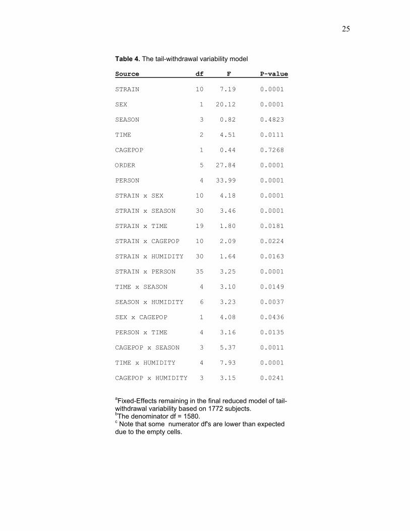
withdrawal latency from which LS means were derived are presented in Table 4. These

LS means are presented along with analogous raw means in Table 5. Figure 2 illustrates

the intriguing but complex effect of season and vivarium humidity on thermal nociceptive

sensitivity.

2.3.4 Controlled experiments. ANOVA was performed on the five-factor (strain x sex x

time x experimenter x order) design. This analysis, presented in Table 6, was used to

partition the trait variance among genotypic, environmental and gene by environment

interaction sources. Sex is represented as a genotype by environment factor, although

this status is debatable. Regardless of whether sex is considered a purely environmental

factor, a purely genetic factor, or an interaction, in this case the influence of sex by itself

is miniscule (0.4%); it is the sex by environment interactions that account for 7.9% of the

variance. Collectively, Figure 3 shows that 87% of the total sums of squares in this

experiment could be explained by genotype (27%), environmental factors (45%) and

25

Table 4. The tail-withdrawal variability model Source df F P-value STRAIN 10 7.19 0.0001

SEX 1 20.12 0.0001

SEASON 3 0.82 0.4823

TIME 2 4.51 0.0111

CAGEPOP 1 0.44 0.7268

ORDER 5 27.84 0.0001

PERSON 4 33.99 0.0001

STRAIN x SEX 10 4.18 0.0001

STRAIN x SEASON 30 3.46 0.0001

STRAIN x TIME 19 1.80 0.0181

STRAIN x CAGEPOP 10 2.09 0.0224

STRAIN x HUMIDITY 30 1.64 0.0163

STRAIN x PERSON 35 3.25 0.0001

TIME x SEASON 4 3.10 0.0149

SEASON x HUMIDITY 6 3.23 0.0037

SEX x CAGEPOP 1 4.08 0.0436

PERSON x TIME 4 3.16 0.0135

CAGEPOP x SEASON 3 5.37 0.0011

TIME x HUMIDITY 4 7.93 0.0001

CAGEPOP x HUMIDITY 3 3.15 0.0241

aFixed-Effects remaining in the final reduced model of tail-withdrawal variability based on 1772 subjects. bThe denominator df = 1580. c Note that some numerator df's are lower than expected due to the empty cells.

26

Table 5. Influence on thermal nociception of individual levels of genetic and environmental factors.

Factor Raw Datab N LS Meansc N Experimentd N Levela (s) (s) (s) Experimenter BM 2.5 (0.03) 828 2.6 (0.18) 166 JH 2.3 (0.04) 482 2.0 (0.21) 213 JM 3.6 (0.02) 3376 3.7 (0.36) 505 3.4 (0.12) 96 KM 3.0 (0.08) 190 3.0 (0.20) 21 SW 2.6 (0.02) 2723 2.2 (0.22) 867 2.1 (0.06)* 96 Genotype 129P3/J 3.4 (0.09) 211 2.8 (0.41) 95 A/J 3.6 (0.08) 368 2.8 (0.24) 187 3.2 (0.15) 64 AKR/J 3.0 (0.07) 250 2.2 (0.22) 161 BALB/cJ 3.8 (0.09) 276 3.8 (0.34) 138 C3H/HeJ 2.4 (0.06) 214 2.4 (0.16) 408 C57BL/6J 2.5 (0.04) 744 2.1 (0.11) 108 1.9 (0.07)* 64 C57BL/10J 2.6 (0.06) 278 2.1 (0.11) 133 C58/J 2.7 (0.07) 122 2.5 (0.30) 88 CBA/J 2.6 (0.07) 223 2.4 (0.34) 239 DBA/2J 3.4 (0.05) 563 2.6 (0.16) 129 3.1 (0.14) 64 RIIIS/J 3.3 (0.11) 122 3.0 (0.41) 86 Season *see Fig. 2 Cage Density 1-3 2.9 (0.02) 3577 3.2 (0.35)e 939 4-6 3.1 (0.02) 4194 2.0 (0.33) 833 Time of Day 08:00-10:55 h 3.2 (0.04) 863 3.1 (0.35) 284 2.9 (0.13) 96 11:00-13:55 h 3.1 (0.02) 3746 2.2 (0.24) 894 14:00-17:00 h 3.0 (0.02) 3169 1.8 (0.27) 594 2.5 (0.10)* 96 Sex Female 2.9 (0.02) 4109 1.9 (0.30) 888 2.7 (0.12) 96 Male 3.2 (0.02) 3766 2.1 (0.32) 884 2.8 (0.12) 96 Humidity *see Fig. 2 Order of Testing 1st 3.2 (0.02) 2649 2.3 (0.36) 642 3.0 (0.19)f 48 2nd 3.0 (0.02) 2386 2.0 (0.32) 567 2.8 (0.18) 48 3rd 3.0 (0.03) 1744 1.9 (0.30) 359 2.6 (0.16) 48 4th 3.0 (0.04) 936 2.1 (0.31) 204 2.5 (0.15) 48 Values represent mean ± S.E.M. 49°C tail-withdrawal latencies. aOnly levels analyzed in the linear model are presented. bRaw data (n = 8034) from the full archival data set. cLeast squares (LS) means from a subset of data points (n = 1772) from 2000-2001. dMeans from a fully-crossed and -balanced experiment (n = 192) of May 15, 2001. eLS means suggested that this factor may affect tail-withdrawal latencies in male mice only. fA trend towards significance was obtained (p = 0.14); but see Fig. 4. *Significantly different from all other levels, p<0.05. No attempt was made to assess the significanceof group differences from the raw data or LS means.

27

4.04.0 4.0 4.0

<20% 20-39% 40-59% >60%2.0

2.5

3.0

3.5Spring

<20% 20-39% 40-59% >60%2.0

2.5

3.0

3.5Winter

<20% 20-39% 40-59% >60%2.0

2.5

3.0

3.5Summer

<20% 20-39% 40-59% >60%2.0

2.5

3.0

3.5Fall

10

20

30

40

50

60

70

80

0 50 100 150 200 250 300 350

% H

umid

ity

Spring Sum mer FallW inter

Figure 2. Influence of humidity and season on 49°C tail-withdrawal (TW) latencies in 1772 inbred mice. Main graph show vivarium humidity values measured daily at approximately 09:00 h. The trendline represents a moving average of the values. Insets show humidity by season interaction LS means (TW latency in seconds) calculated from these data. Only humidity classes per season with n>30 are shown. As can be seen, tail-withdrawal latencies tend to decrease with increases in humidity, except perhaps in Winter.

28

TESTERxORDER E 2.087 3 0.696 1.942 0.128 0.7970821SEXxTIMExTESTER E 0.775 1 0.775 2.164 0.145 0.2959936SEXxTIMExORDER E 2.695 3 0.898 2.507 0.064 1.0292938SEXxTESTERxORDER E 0.668 3 0.223 0.622 0.603 0.2551274TIMExTESTERxORDER E 0.857 3 0.286 0.798 0.498 0.3273116SEXxTIMExTESTERxORDER E 2.464 3 0.821 2.292 0.083 0.9410686 STRAINxSEX GE 2.079 2 1.039 2.901 0.060 0.7940267STRAINxTIME GE 3.572 2 1.786 4.986 0.009 1.3642440STRAINxTESTER GE 13.853 2 6.927 19.335 0.000 5.2908376STRAINxORDER GE 1.635 6 0.273 0.761 0.603 0.6244510STRAINxSEXxTIME GE 0.271 2 0.135 0.378 0.687 0.1035023STRAINxSEXxTESTER GE 0.088 2 0.044 0.123 0.884 0.0336096STRAINxSEXxORDER GE 0.965 6 0.161 0.449 0.844 0.3685598STRAINxTIMExTESTER GE 0.586 2 0.293 0.818 0.444 0.2238093STRAINxTIMExORDER GE 0.92 6 0.153 0.428 0.859 0.3513730STRAINxTESTERxORDER GE 0.873 6 0.145 0.406 0.873 0.3334224STRAINxSEXxTIMExTESTER GE 2.258 2 1.129 3.151 0.047 0.8623916STRAINxSEXxTIMExORDER GE 2.356 6 0.393 1.096 0.370 0.8998205STRAINxSEXxTESTERxORDER GE 1.659 6 0.276 0.772 0.594 0.6336172STRAINxTIMExTESTERxORDER GE 2.208 6 0.368 1.027 0.413 0.8432953STRAINxSEXxTIMExTESTERxORDER GE 5.114 6 0.852 2.379 0.035 1.9531757 Error 34.393 96 0.358 13.1356220 TOTAL 261.83 100

Table 6. ANOVA from a balanced 5-way design Source Type SS df MS F-ratio P % VarianceSTRAIN G 70.801 2 35.401 98.814 0.000 27.0408280 SEX E 1.065 1 1.065 2.973 0.088 0.4067525TIME E 9.013 1 9.013 25.159 0.000 3.4423099TESTER E 88.971 1 88.971 248.346 0.000 33.980445ORDER E 7.454 3 2.485 6.935 0.000 2.8468854SEXxTIME E 0.012 1 0.012 0.033 0.857 0.0045831SEXxTESTER E 0.000 1 0.000 0.000 1.000 0.0000000SEXxORDER E 1.489 3 0.496 1.385 0.252 0.5686896TIMExTESTER E 0.248 1 0.248 0.692 0.407 0.0947179TIMExORDER E 0.401 3 0.134 0.373 0.772 0.1531528

29

STRAIN

TESTER

TIME

ORDER

ERROR

STRAINxENV SEXSTRAINxSEXSEXxENV

STRAINxSEXxENVENVxENV

Environment 45%

Genotype 27%

Residual 13%

Genotype by Environment 15%

Figure 3. Partitioning the Type I sums of squares of 49°C tail-withdrawal test variability. Shown are percentages of the corrected total variance in a fully-balanced and -crossed study performed on A/J, C57BL/6J and DBA/2J mice on a single day. Sex appears as a genotype x environment factor, although there exists some debate about this status (see text).

30

genotype x environment interactions (15%). The factor level means from the balanced

experiment, and associated significance testing are presented in Table 5. Although an

attempt was made to analyze this balanced experiment using CART, no tree could be

built. CART requires many hundreds of observations and a large number of variables

(Johnson and Wichern, 1998), and this balanced experiment apparently did not have

sufficient data for the analysis.

Figure 4a shows that the effect of even the lowest ranking factor, order of testing, can

be demonstrated in a controlled experiment using a sensitive strain. Of the mice returned

to their home cage after testing, the third and fourth mice have tail-withdrawal latencies

that are significantly different from those of the first mouse to be tested, p < 0.05. In the

group placed in a holding cage after testing, no differences were observed. However, the

fourth mice tested from the home cage group differed significantly from the first mice

tested and their counterparts in the holding cage group. Figure 4b shows the effect of

within cage order of testing on morphine analgesia. Because individual differences in

basal thermal nociceptive thresholds may influence the magnitude of post-drug treatment

latencies, a commonly used measure of analgesic effect is the percent analgesia,

%100×

−

−=

latencytreatmentprelatencycutoff

latencytreatmentprelatencytreatmentpost% analgesia

Analgesic doses (AD50s) are higher in the fourth mouse tested than in the other groups, p

< 0.05. No significant population effects were observed in the ANOVA (strain x sex x

population) though strain (p < 0.001) and sex (p < 0.025) differences were replicated, as

shown in Table 7.

31

3

4

5

6

7Home Cage

Holding Cage

*•

1st 2nd 3rd 4th

Order of TestingTW

Lat

ency

(s)

a

b

0

20

40

60

80

100 1st (AD50: 14.2 mg/kg)2nd (AD50: 16.6 mg/kg)3rd (AD50: 17.2 mg/kg)4th (AD50: 22.0 mg/kg) *

5 10 20 40

Morphine Dose (mg/kg)

% A

nalg

esia

Figure 4. a. Influence of within-cage order of testing in Swiss-Webster (SW-Sim; Simonsen Labs) mice. Symbols represent mean (±S.E.M.) 49°C tail-withdrawal (TW) latencies of mice tested and then immediately returned to their home cages or transferred to a holding cage after testing. *Significantly different than 1st mice, p<0.05. •Significantly different than 1st mice and Holding Cage (4th) mice, p<0.05. b. Order of testing effects on morphine analgesia.

Table 7. ANOVA from the strain, sex and population experiment. Sum-of- Mean- Source Squares df Square F-ratio P-value STRAIN 17.133 2 8.567 22.433 0.000 SEX 0.960 1 0.960 2.514 0.117 CAGEPOP 0.375 1 0.375 0.982 0.325 STRAINxSEX 3.427 2 1.713 4.487 0.014 STRAINxCAGEPOP 0.498 2 0.249 0.652 0.523 SEXxCAGEPOP 0.143 1 0.143 0.373 0.543 STRAINxSEXxCAGEPOP 0.643 2 0.321 0.841 0.435 Error 32.079 84 0.382

32

2.4 Discussion of the environmental impact on thermal nociceptive sensitivity

In more than 10 separate strain surveys of 49°C tail-withdrawal sensitivity

performed in our laboratory each using a common set of 12 inbred strains, broad-sense

heritability has been estimated to be between H2 = 0.21 and 0.41 (Mogil et al., 1999a). In

the large archive, the heritability is estimated at approximately 0.241, and in the

controlled experiment it is estimated at 0.35. This leaves a clear majority of the variance

to be explained by factors other than genotype, even if this estimate may be negatively

biased due to the presence of the many other factors in the data set that were not fitted in

the heritability analysis. The five-factor experiment performed here indicates that

individual differences on this trait are largely due to environmental factors and genotype

by environment interactions. Modeling also demonstrated that all environmental factors,

with the exception of order, interact significantly with genotype.

The information from the original data archive is highly confounded because it

contains numerous empty cells and heavily unbalanced data. Therefore the CART

results, raw means and LS means must be interpreted cautiously, and where possible

confirmed by experiments in which levels of each factor are systematically varied in

balanced designs. CART analysis reveals that the most important predictor of tail-

withdrawal latency is experimenter, followed by genotype and season. Strain effects are

no surprise (Mogil et al., 1999a), but it is interesting to note that the effect of

experimenter is greater than that of strain in both the data mining and controlled

experiments. The importance of experimenter is generally in agreement with the recent

findings of Crabbe and colleagues (1999), who simultaneously tested a common set of

33

mouse strains on a number of behavioral assays using identical methods in different sites.

Although the relative ranking of the strains in that study was similar at each site, the

absolute performance differed greatly from site to site. This variability can only be

accounted for by factors not explicitly controlled for, notably including the specific

experimenters in each laboratory. An important aspect of many pain tests is the

necessary use of restraint, which can produce stress-induced analgesia (SIA), either to

perform the test and/or to administer analgesic drugs. Genetic influences on the amount

of SIA have been demonstrated (Panocka et al., 1986; Mogil et al., 1996). Differences in

restraint method (Plexiglas chamber vs. cloth cardboard holder) can result in large

differences in the tail-withdrawal latency (Mogil et al., 2001), but subtle differences in

the manner in which each experimenter restrains mice may be a sufficient source of

experimenter differences. It should be noted that this is not the only possible source of

experimenter effects, which may include pheromonal cues, scents, reaction time, and the

ease with which mice are removed from the cage for testing. For experimenter, genotype

and time of day factors, the influence of factors suggested by the raw data and LS means

were confirmed as significant. Our finding of decreased latencies (i.e., increased

sensitivity) in the afternoon may be in contrast to some rodent data obtained using the

hot-plate test (Kavaliers and Hirst, 1983; Wesche and Frederickson, 1981), but appears to

agree with at least some data obtained in humans (Folkard et al., 1976; Kleitman, 1963;

Zahorska-Markiewicz, 1988).

Season was another factor ranked highly by CART. This factor is difficult to

study in a controlled fashion, requiring at least 2-3 years of observations to truly

demonstrate a circannual pattern. It may be possible to identify a data subset from the

34

archive to achieve this statistically. One major concern is that seasonal cues should be

absent from the controlled light cycle of the animal colony, but such cues apparently may

remain. Notably, climate records reveal temperature to be well controlled, but humidity

fluctuating freely in the animal colony (Figure 2) in a manner that could cue season.

However, the effect is not simple, with season and humidity interacting significantly in

the data archive (Table 4). Nociceptive threshold least-squares means are generally

higher in low humidity, regardless of season (Figure 2). This is in agreement with human

clinical data (Aikman, 1997) from which an apparent increase in pain sensitivity in

conditions of high humidity is observed. While this appears to be at odds with work by

Patberg et al., (1986), the latter work was based on self-report, which do not agree with

measured clinical scores in the large-sample seasonal study by Hawley et al. (2001). It

also appears as though in the laboratory mouse, nociceptive thresholds are elevated in the

spring and summer and lower in the fall and winter, in agreement with Hawley et al.

(2001), though the lack of occurrence of all humidity levels for all seasons in the present

study makes such comparisons difficult to make. It is highly likely that other factors are

correlated with these observations, including tester and strain, particularly when one

considers that all of the data from a particular day, and thus possibly a bulk of the data

from a particular humidity can come from a single experimental run by a single tester.

Efforts are underway to directly manipulate humidity within season to try to isolate the

confounded effects of season and humidity.

For sex and order of testing, trends in the same direction as the LS means were

seen, but significant differences were not obtained in these strains and with this sample

size, attesting to the relatively low impact of these factors. The sex difference observed

35

in CART, with males less sensitive to thermal pain than females, is in agreement with

previous findings by other investigators in independent studies (Berkley, 1997) and in our

own work (Mogil, 2000), though these latter data are a small subset of the data archive,

so agreement might be expected. It should be noted that though the sex difference

observed in the five-factor experiment is small, sex by environment interactions account

for an appreciable amount of variance. This may be indicative of the operation of sex as

a genotype by environment factor, in which the genetics that produce biological sex

differences result in differential sensitivity to environmental factors. Though this appears

to be incompatible with the consistency of the sex differences observed in the CART

analysis, it is not. The interaction occurs because for this trait and the mice studied

herein the magnitude of sex differences varies in different environmental contexts, but

not the direction, thus a consistent direction of sex effects is observed in the regression

tree.

The order effect, a previously unknown influence on nociceptive sensitivity, can

be eliminated by preventing the exposure of naïve mice to previously tested mice. This

suggests that mice are somehow signaling their cage mates, likely through release of

pheromones or via ultrasonic vocalizations. The relevance of order effects to pain

research is magnified by our observation that measurements of the efficacy of five

different analgesics are even more greatly affected by order of testing, with the first

mouse tested from a cage as much as 50% more sensitive to the drug than the fourth

mouse (Figure 4b).

Cage population density effects, though present in the LS means and ranked as the

fourth most influential by CART were not seen in a controlled experiment. There are

36

several possible explanations for this. The high ranking of the factor in CART may be

due to the fact that all levels of population were considered separately in this analysis,

whereas they were collapsed in the fixed effects modeling. Indeed, when CART was run

on the same data with population collapsed into a two category factor, this factor was

ranked seventh in importance, while all other factors remained in the same relative

positions as shown in Table 8. In the controlled experiment we only compared cage

populations of two and four mice per cage, and while these are representative of the two

population categories in the modeling study, they are not the extreme conditions of cage

population. We did not want to include a condition in which mice were in social

isolation, as this may be a qualitatively different phenomenon than the relative crowding

conditions that we sought to study. In agreement with modeling findings, however,

increased tail-flick latencies to radiant heat have been observed in rats and mice housed

alone (Gentsch et al., 1988; Naranjo and Fuentes, 1985; Puglisi-Allegra and Oliverio,

1983). Also, the two-week period of acclimation to housing may not have been

sufficient. Many of the mice in the archive are grouped at weaning into various

populations based in part on litter size, which may be influenced by strain related and

seasonal fecundity. These correlated factors may have influenced the cage population

effects obtained in the archive analysis. Another possibility is that population effects

may be due to the presence of mice with high test order in the data archive for high cage

populations. Because we performed the holding cage manipulation described above, the

order effect would not be present in this experiment.

The results from data mining are corroborated by many previous studies in which

these factors or similar factors were directly investigated. However, there are few

37

Table 8. Factor importance rankings with population collapsed into a two-

category variable.

Factor Number of Levels Score

Experimenter 11 100.0

Genotype 40 75.8

Season 4 36.2

Time of Day 3a 14.9

Sex 2 14.1

Humidity 4b 12.0

Cage Density 2c 10.1

Order of Testing 7 7.3

aTime of day levels were: early (09:30-10:55 h), midday (11:00-13:55 h), and late (14:00-17:00 h). bHumidity levels were: high (≥60%), medium-high (40-59%), medium-low (20-39%), and low (<20%). cCage Density levels were: low 1-3 and high 4-6.

38

comparable studies in which all or even a subset of these factors are considered together.

The higher order interactions of these factors observed in the five-way experiment are

quite difficult to interpret biologically in any detailed sense, and the possibility of

observing five-way interactions is a risk of considering so many factors simultaneously.

This approach allowed us to partition the sums of squares in the most naturalistic

situation possible--perhaps a benefit that outweighs the problem of interpretation this

created. Strain by time, strain by sex and strain by tester interactions may be interpreted

in terms of various genetic factors segregating in the strains studied here, each potential

sites of differential interaction with the environment.

Overall, the present study demonstrates that for a bio-behavioral trait such as

thermal pain responsiveness as tested in a modern pain research laboratory, it is possible

to identify both genetic and environmental factors associated with trait variance.

Certainly, the ability of some of these factors to affect nociception in rodents and humans

has been noted previously. Ultimately, the operation of all the factors considered herein

needs to be further explicated with mechanistic studies in mice and humans. We expect

that for a number of laboratory environmental factors, stress level may be a common

mediator, given the well-known ability of environmental stressors to modulate pain

sensitivity in either direction depending on its parameters (Jorum, 1988). The present

findings also have immediate implications for current attempts to identify genes relevant

to complex traits like pain. Given that an overwhelming proportion of variability in

nociceptive sensitivity is accounted for by environmental factors and their interaction

with genes, the mere elucidation of pain genes will not succeed in explaining the nature

of individual differences. Once the relevant genes are found, however, systematic

39

investigation of gene by environment interactions may yield clinically important

information leading to the individualization of pharmacologically- and behaviorally-

based treatment strategies.

On a broader note, this study suggests that even when laboratory environmental

conditions are assumed to be “controlled” to the standard of the existing literature,

serious sources of environmental variability exist. Many of these have a measurable

effect on behavior, even in small studies. Though the genetic similarity of inbred strains

allows for comparison of data within and across labs, such studies must be done with

consistency of environmental conditions in mind. This is particularly true for the study

of behavioral traits, which are largely determined by environment and gene-environment

interactions.

40

3. Development and Evaluation of a Haplotype Based Computational Algorithm for

the Genetic Analysis of Behavioral Traits in Inbred Mouse Strains The genetic analysis of behavior is typically achieved through two major

approaches. One is the breeding of targeted or spontaneously arising mutant organisms,

where the assumption is that the effect of a single altered gene can be studied in an

organism by comparison to controls with an intact (“wild type”) gene. The other is the

detection of genomic regions associated with phenotype. These regions, called

quantitative trait loci, are identified by associating phenotypic values with genotypes at

markers of known location. Both of these approaches have benefits and limitations, and

ideally should be used in concert (Belknap et al., 2001). The generation of mutant strains

necessarily involves confounding effects of genetic background that can influence studies

of pain related phenotypes (Lariviere, Chesler and Mogil, 2000). Compensation often

occurs when mutations are present, further obscuring interpretation of findings.

Furthermore, this approach is inefficient if one has no a priori hypothesis about the role

of the mutated gene in question, or about which genes are involved in a given behavior.

The detection of QTLs is a method that allows one to identify multiple regions of genome

in which genotype associates with phenotype, implying the presence of trait-related genes

in these regions (Lander and Schork, 1994). This method requires no a priori

assumptions about the number of genes involved or their functions, allows for assessment

of epistatic interaction of genes, employs phenotypic assessment in mice that may be less

“abnormal” than mutants (although are certainly not well representative of wild mice),

and is unaffected by compensation-related confounds.

41

The typical approach to QTL mapping is a time consuming and resource intensive

process, and the result is the detection of large regions of the genome associated with a

trait that may contain many hundreds of genes. Finding the actual genetic basis of the

QTL has been described as a “long road” (Nadeau and Frankel, 2000) and critics have

argued that the journey may be futile. At best, the process of going from a detected QTL

to knowledge of the underlying genetic polymorphism or even the affected gene(s) is

sufficiently difficult as to make false positive QTL detection a serious issue. Alternatives

and enhancements to QTL mapping have been proposed to increase the precision and/or

decrease the effort of the process. Any proposal must be considered with the impact of

false positives firmly in mind.

An interesting emerging methodology for QTL detection is in silico mapping

(Grupe et al., 2001). This approach capitalizes on known genetic differences between

inbred organisms to identify QTLs rapidly in a genetically diverse population using a

rapid computational process, thereby eliminating the need to genotype individual mice.

However, serious concerns about the present statistical power and error rate of this

method have been raised (Chesler et al., 2001; Darvasi, 2001). Though this method has

been hailed as a significant advance, thorough evaluation is necessary before any

widespread practical application of the technique is made.

3.1. QTL mapping using experimental crosses Genetic linkage mapping studies in mice begins with definition of a phenotype,

determination that it is quantitatively distributed, and demonstration of heritability of the

trait through phenotypic assessment in a panel of inbred strains. This has been

42

accomplished for many pain-related phenotypes (Mogil et al, 1999a). From these “strain

surveys,” a pair of extreme-responding strains is chosen, and cross-mated to create an F1

hybrid generation of heterozygotes. These F1 progeny are subsequently crossed, resulting

in an F2 hybrid generation in which individuals can be heterozygous or homozygous for

either allele at any genetic locus. The phenotypes are assessed in each individual F2

mouse. Genomic DNA must then be extracted and amplified at markers known to be

polymorphic between the parental strains, so that the genotype of each strain can be

determined at marker loci spanning the genome. The association of marker genotype and

behavioral phenotype is determined using a variety of statistical methods that allow

estimation of the position of quantitative trait loci and/or the magnitude of their effects.

The present work describes development and evaluation of in silico mapping

techniques that can be used to identify QTLs using data that comes directly from

phenotypic study of inbred strains of already-defined genotype at a large number of

informative markers, thereby eliminating (or reducing) the need for generation of an

experimental cross. Such a technique can be employed easily by researchers who have

greater expertise in the phenotypic evaluation of complex traits than in molecular

techniques, and takes advantage of more polymorphic information than methods

comparing only two strains can. The results can either be used directly prior to candidate

gene testing or to identify regions in which high-density genotypic analysis of a cross

should be performed to reduce genotyping expense while increasing precision.

3.1.1 Some QTL mapping concerns. There are several criteria by which novel mapping

methods can be evaluated, particularly with respect to the way they address some of the

43

drawbacks of performing genetic mapping in experimental crosses. One of the primary

motivations for developing computational alternatives to the use of an experimental cross

is that crosses are expensive and time-consuming endeavors due to the massive amount

of genotyping that is required. These practical concerns limit widespread employment of

a rather useful method to a small pool of researchers. For a mouse study, over 250 mice

must be tested for moderately heritable traits (Lander and Botstein, 1989), and

approximately 150 PCR reactions per mouse must be performed and visualized for

maximal resolution (Darvasi et al., 1993). While technology is improving to do this more

efficiently (e.g., by pooling DNA, and via automated visualization of PCR products), the

cost is high, and a reasonable amount of technical facility is still required.

The experimental cross requires generation of genetically unique progeny from

two progenitor strains, with each phenotypic measure typically taken from a single

assessment of each mouse. This makes the method highly susceptible to "phenocopy,"

environmental factors influencing the phenotype in a manner that resembles (and may be

mistaken for) genetic effects. It should be noted that while the use of single phenotypic

observations makes one susceptible to error from imprecise measurement and phenocopy,

F2 crosses are fairly robust and infinitely high sample sizes are possible for both

genotypic and phenotypic data to reduce the impact of this problem. Any alternative

method to the F2 cross ought to be similarly robust, with results not greatly altered by

omission of a single phenotypic or genotypic value. Repeated measures can be used in

many cases to increase precision of phenotypic measurement, but for some traits, carry-

over effects render this impossible. Although accounting for the covariance of repeated

measures can alleviate this problem for some traits, it is often not feasible. This is a

44

major source of concern in the assessment of behavioral traits, and particularly in the

influence of drug effects on those traits. It is conceivable that there exists genetic

variability in the impact of repeated measure effects, which could mask or exaggerate the

influence of genetics on the trait of interest. Experimental crosses also cannot be used

where measurements from separate control groups are required. For some traits, only a

single measure in each individual is possible. This is true for any pain tests that cause

permanent tissue damage (e.g., the formalin test), in which there is learning that occurs

after multiple exposures to the noxious stimulus (e.g., the hot-plate test), or in the many

traits of interest to neuroscientists that involve group comparisons of measurements made

through terminal procedures (e.g. anatomical traits). Using grand-progeny designs

(Weller et al, 1990), one can improve the precision of phenotypic measurement or

consider group comparisons where only single observations can be used, but while

decreasing variability between genetically similar groups this greatly increases the

volume and complexity of the study because of the increased genetic variability within

groups.

A major drawback of experimental crosses is that only those regions that are

polymorphic between the two progenitor strains can be identified as QTLs. Using two

different pairs of progenitor strains in separate crosses each with high statistical power,

different QTLs have been observed for the same behavioral trait assayed in the same

laboratory (Hitzemann et al., 2000). Thus, any mapping system based on only two inbred

strains, particularly if they are not strains with extreme phenotypes, is likely to under-

report QTL number because some QTLs are not segregating in the mapping population.

45

A benefit of using the F2 cross is that both additive and dominance related genetic

effects can be estimated because heterozygous mice are present in the study. In the use

of methods based on inbred strains, mice are homozygous at every locus, rendering the

assessment of dominance effects impossible. This precludes the detection of hybrid

vigor, in which having one copy of each allele confers an advantage over homozygous

status at either allele.

QTL mapping has often been criticized because of its low resolution (Nadeau and

Frankel, 2000). Often a 20 centiMorgan (cM) or larger region of genome is identified as

the QTL confidence interval. A region of this size can contain large quantities of genes,

and thus one is left to perform positional cloning or with an excessive number of

candidates to test. However, positional cloning requires that the candidate region be

reduced to approximately 0.5 cM (Rikke and Johnson, 1998). Part of the resolution

problem is due to linkage of markers in close proximity, particularly when single-marker

analyses are utilized. Results from adjacent markers are correlated in these analyses,

therefore in regions surrounding the QTL, high associations with the phenotype are also

observed. Interval mapping reduces this problem by estimating the likelihood of a QTL

between pairs of markers, allowing for estimation of both the position and effect of the

QTL. Composite interval mapping is a further enhancement, which allows for

consideration of the effects of background markers that may artificially elevate or

decrease apparent QTL effects. Though more sophisticated methods of analysis such as

interval mapping and composite interval mapping do help to improve resolution, QTL

confidence intervals are still large. A substantial increase in sample size, with a resulting

increase in frequency of genetic recombination can further improve precision, though this

46

is impractical for widespread use and may be subject to diminishing returns. Other

approaches to more precisely estimating the QTL position have also been attempted,

including the use of advanced intercross lines (Darvasi and Soller, 1995), generating new

congenic strains, or narrowing the possible interval with testing of existing overlapping

knockouts and congenics containing differing amounts of “hitch-hiking” genetic material

linked to the region of interest (Flaherty and Bolivar, 2002).

The required statistical thresholds for QTL mapping techniques involving whole

genome scans has been the topic of extensive debate, particularly since the publication of

theoretical minimum logarithm of the odds (LOD) scores by Lander and Kruglyak

(1995). The major issue is that mapping techniques by their nature employ multiple tests,

and the family-wise error rate is thus potentially very high. However, the typical

hypothesis considered in the family of tests would be that there is no QTL present in the

entire genome, a hypothesis of virtually zero probability in a heritable trait. Thus,

correcting strictly for the number of tests employed is not appropriate in some cases,

particularly because tests on linked markers are not independent. The use of resampling

techniques, in particular permutation tests, is a widely used error-control technique

(Churchill and Doerge, 1994). This technique may be employed to control the marker,

chromosome or genome (experiment) error rate. Another approach for controlling error

rates that has been employed in QTL detection is Benjamini and Hochberg’s (1995)

procedure to control the false discovery rate (Mosig et al. 2001). This method is more

powerful than Bonferroni correction.

Reliability of QTL mapping is also a concern. Although the number of subjects

in a typical F2 cross allows sufficient power to detect at least one QTL in the whole

47

genome, typical quantitative traits may be determined by several genes. With minimal

power, at least one of these may be detected by chance, and the amount of variance this

single QTL accounts for is generally over-estimated. A second mapping study in the

same population may detect a different QTL. Other non-trivial reasons for the lack of

replication of QTL studies include differences in polymorphisms present in different sets

of progenitor strains, epistatic interactions, gene-environment interactions, and

inconsistent definition of the phenotype (Roubertoux and Le Roy-Duflos, 2001).

3.2. Alternatives to experimental crosses

Techniques are in use or under development to address these concerns with and

limitations of mapping with recombinant crosses. Several of these techniques involve the

analysis of haplotypes (genotypes of inbred strains in which both alleles are identical).

The practical and statistical issues outlined above should be used to assess the value of

these methods, particularly as they compare to the more commonly employed F2 cross

approach to mapping.

3.2.1. Recombinant inbred strains. An inexpensive technique—once the resource has

been generated—for the preliminary determination of QTL location is the use of

recombinant inbred (RI) strain sets (see Gora-Maslak, 1991). In the creation of these

strains, two inbred progenitor strains are crossed to create F2 hybrids, which are then

inbred for 20 generations creating a set of inbred strains that feature one or the other

homozygous parental genotype at each locus. Because the resulting RI strains have

assorted genetic material at each locus, the association of genotype and phenotype can be

accomplished simply by using databased marker information from a previous genotypic

48

survey of the RI strain panel. The genotypes and phenotypes are correlated in a point-

biserial fashion at each marker. Because this method employs mice homozygous at all

loci, no dominance effects can be identified; only additive genetic effects can be

estimated. Single marker approaches such as these have low resolution because of the

presence of linked markers. If a marker is associated with a trait, all markers linked to it

(potentially all markers on the chromosome), will show elevated linkage to that trait. The

method also has no ability to resolve linked QTLs in coupling phase (linked increasor

alleles), and will miss QTLs in repulsion (a linked increasor and decreasor allele).

Furthermore, the phenomenon of “mirroring” of QTLs—the identification of QTLs at all

loci that have a common strain distribution pattern, regardless of whether or not the locus

is linked to the actual polymorphism underlying trait variability—can generate numerous

false positive results, particularly when the number of strains is limited. Because the

markers are not genes, and are typically ‘junk’ DNA, they themselves cannot have a

biological effect on the quantitative trait. Thus, the marker itself is not the QTL, and

because recombination between the markers is not being considered, positional

information cannot be estimated using single marker analyses. Power and resolution are

somewhat limited by the number of RI strains available, and the number of RI strains one

is willing to test. However, there is an effort to improve the genetic diversity and

resolution of the RI resource (Williams et al., 2001), which can dramatically increase the

utility of this method and reduce genotyping efforts. Researchers wishing to use this

resource are practically limited to using existing RI strain sets, given the time and effort

required to create new ones, and the progenitors of existing sets may not be the extreme

responders for any particular trait. Not using extreme responding strains limits the

49

number of large effect magnitude QTLs that can be identified. Furthermore, as with F2

hybrids, the alleles of only two strains are considered in RI-aided mapping, so the only

QTLs that can be identified are those for which a polymorphism between the two strains

exists. However, RI strains remain a very useful tool for behavioral genetics, because

genetically identical individuals can be tested separately in a variety of environmental

contexts. Replication studies and comparison studies are also facilitated by the

retrievability of the genetic resource.

3.2.2. The heterogeneous stock: A method to increase resolution and account for

increased genetic diversity F2 crosses are limited both in their resolution and in the

number of actual QTLs that may be identified. This is both because the density of

themselves markers that one can employ is restricted to those that are polymorphic

between a pair of strains, and because the genes underlying the phenotype must be

polymorphic. One promising technique for increasing the resolution of QTL mapping

and for allowing the detection of more QTLs through increased genetic diversity is the

use of a heterogeneous stock, one of which has been established through out-breeding of

8 inbred mouse strains (Talbot et al, 1999). In the earliest use of this technique, general

linear models with allele as a grouping variable were fitted at each marker (Talbot et al.,

1999), but later developments have improved precision through the use of multipoint-

mapping, which takes into account the presence of linked markers and includes

information about progenitor haplotypes (Mott et al., 2000). Strictly using the marker

allele in the single marker approach employed in Talbot et al. (1999) was less successful

than this latter method because the alike-in-state markers may not have been identical by

50

descent, an important consideration for the development of marker based in silico

mapping. Though the HS technique provides greater resolution and genetic diversity

than a single experimental cross, the approach requires the generation of unique progeny

and thus necessitates the use of high-density genotyping, and is again not easily amenable

to the study of traits that require multiple measures from different individuals.

3.2.3. Inbred strain survey-based haplotype mapping. Employing the genetic variability

and marker density afforded by use of a set of inbred strains, and the use of databased

marker information, it may be possible to map QTLs in the mouse using only the data

from inbred strain surveys. This is because the inbred strains are derived from a small

number of progenitor strains, for which genealogical information has been well cataloged

(e.g. Beck et al., 2000). When strains have like alleles of polymorphic genetic markers, it

is highly probable that these alleles are of common origin (i.e., identical-by-descent

[IBD]). In this case, identical marker alleles are likely to be co-inherited with identical

gene alleles. One example, microsatellite markers, are untranslated DNA found

dispersed throughout the mammalian genome for which primers can be developed, but

which have varying lengths of DNA between strains. The microsatellite marker

polymorphisms have been demonstrated to be related to lineage in that more distally

related strains have fewer microsatellite alleles in common (Schalkwyk et al., 1999).

However, the results of Mott et al. (2000) for heterogenous stock based mapping

demonstrate that this assumption may be problematic, and that it might be necessary to

incorporate a measure of probability of identity by descent for improved quality of

mapping from a diverse population.

51

The strain distribution pattern (SDP) of marker genotypes can be used in models

of phenotype-genotype association. Such a technique has the potential to be very high

resolution, inexpensive and rapid. Because marker-type-specific genotyping methods are

not required in a computational method using databased information, any type of marker

or even gene can be used, provided that polymorphisms in a number of inbred strains

have been identified. Furthermore, no proficiency with molecular techniques is required,

making the technique accessible to researchers whose greater expertise lies in the

evaluation of complex phenotypes.

3.3 Evaluation and further development of “ in silico” QTL mapping methods

A variety of different analytic approaches can be used on several existing genotypic

databases to characterize and identify those methods that are most fruitful. There are a

number of aspects to consider: 1) selection of an algorithm, 2) selection of a database or

combination of databases, 3) potential incorporation of genetic origin information, 4)

smoothing and visualization of output, 5) appropriate handling of dependent (linked)

markers, 6) peak detection and significance thresholds. This is clearly a non-sequential

process, and much optimization will be necessary to create a viable method of in silico

mapping. In the present study, statistical power of two different mapping approaches is

considered, and methods of peak detection are compared. Reliability in comparison to

genome-wide scans based on genetically diverse experimental crosses is evaluated.

52

3.3.1 Two approaches to in silico mapping. Grupe et al. (2001) have recently published a

method of trait mapping based on the use of the inbred strain distribution of single

nucleotide polymorphisms (SNPs). Briefly, pairwise strain differences in genotype are

calculated for each SNP, and these are summed in 30 cM intervals each shifted by 10 cM.

This produces arrays of genotypic differences which are then correlated with pairwise

phenotypic differences. This method is flawed, and likely not to perform well in practice

as originally described (Chesler et al., 2001; Darvasi et al., 2001). It has limited

resolution because of the large size of intervals created, and is heavily biased by the

presence of linked markers because genotypic differences are summed over these

intervals. Thus, more SNPs in an interval, even with identical SDPs, create the

appearance of greater genetic diversity in that interval. This will increase the probability

of observing a high correlation in that interval, where as in other intervals, correlations

may be constrained to be low. This is problematic because a single SNP might be the

cause of trait related polymorphisms, but will be unobservable if present in an interval

with constrained correlation. The creation of overlapping intervals might result in the

artificial appearance of increasing genotype-phenotype association approaching the

putative QTL, because of the correlation of analyses between adjacent intervals.

However, in practice adjacent intervals often have widely disparate results because of the

bias in observable correlations.

A major problem for the use of this technique for behavioral studies is that the

majority of SNP polymorphisms are between the CAST/Ei strain and all other strains.

Thus, the bulk of genetic variability considered in this analysis is that of differences

between CAST/Ei and other strains. CAST/Ei is not only an outlier in genotype—it is

53

also behaviorally distinct from other mice (Le Roy et al., 1998). The method is

absolutely not robust to the removal of this single strain, resulting in catastrophic effects

on QTL detection. This occurs because the addition of a single strain results in many

additional pairs of strain differences. When an outlier strain such as CAST/Ei is added, a

large number of high magnitude genetic and phenotypic differences are added to the

analysis, boosting the potential correlation observable in each interval. However, this

lack of robustness can be informative, if one considers that the inconsistency of results is

indicative of the different sources of polymorphism in the analysis. CAST/Ei is a wild

derived inbred strain, and its differences from more recently developed inbred strains are

reflective of old polymorphisms that may occur in the natural environment. The later

developed strains have mutations that might only be viable in the laboratory--potentially

less relevant to the human polymorphism they aim to model.

The method proposed by Grupe et al, (2001) also has a very high rate of false

positives. The low statistical power of this method is artificially inflated through the

calculation of pairwise differences resulting in correlations with 22 degrees of freedom

from a set of only eight strains. To avoid this issue, a non-statistical approach is

suggested for the detection of positive results (Grupe et al, 2001). Although the reported

validation of the method shows significant agreement with previously published data

(Grupe et al., 2001) this analysis is biased by heavily unbalanced number of true negative

results in comparison to the number of false positive, false negative and true positives,

and further flawed by the determination of significance threshold without consideration

of the pooling of comparison from many separate studies.

54

A method that uses allele as a grouping variable in a linear model is theoretically

more appropriate and meaningful in the context of other mapping methods because the

assumption that one is testing linear relationships is more likely to be valid. The amount

of polymorphism in a region should not be linearly related to the phenotypic difference as

assumed in Grupe et al. (2001), unless one predicts multiple trait related genetic

polymorphisms in each interval, each having an equivalent additive effect on the trait. In

contrast, using linear models with allele based grouping, the additive allelic effect can be

estimated from the single marker analyses, but clearly no such relationship can be

determined from the pairwise-difference approach. The estimation of this additive effect

is useful in the assessment of candidate genes, allowing one to determine whether or not

the effect size of a manipulation is reasonable for the magnitude of effect the

polymorphism produces. The allele-grouping based approach herein proposed is also

advantageous because it is a potentially high-density technique. At any marker or even

gene in which at least multiple strains belong to each of at least two genotypes, a group

comparison can be performed.

3.3.2 Selection of a database. In silico mapping requires the existence of known genetic

information across a large number of commonly used inbred strains. Polymorphism data

is freely available for a number of strains, shown in Table 9, including a table of over

6500 microsatellite markers from the MIT Whitehead Genome Center (Dietrich, 1996;

Copeland, 1993), 128 markers available from a study which included the genotyping of

four additional strains (Schalkwyk et al., 1999), and 300 microsatellite markers

genotyped in over 50 strains by Center for Inherited Disease Research (CIDR). Another

55

marker type for which extensive databased information is becoming available is single-

nucleotide polymorphisms (SNPs). At present, 2948 SNPs have been mapped by MIT

(Lindblad-Toh et al., 2000), and an additional set of 500 SNPs have been added by Grupe

et al. (2001). Proprietary databases are being created with high density SNP information

for several inbred strains. SNPs may be more appropriate for use in these computational

techniques because they can occur anywhere in the genome, potentially affecting

phenotype directly by occurrence within enhancer regions, promoter regions or even

genes. However, many of the presently identified SNPs are not located in genes, and

their use in intervals in the pairwise difference method likens them to markers associated

with trait-relevant polymorphisms. The CIDR database can be used to investigate genetic

background, though the resolution expected from this database is limited. Currently,

because of the small number of genotyped strains with corresponding phenotypes, it is

difficult to incorporate genetic origin information into these analyses. The CIDR

database has high sample size, but low marker density compared to the MIT database.

Microsatellites currently offer much higher resolution than the SNP database because of

this high marker density, but statistical power is low. Current genotyping efforts will

increase statistical power even more, and SNPs, once genotyped in a large enough sample

of mice, could be used as a more relevant source of genetic information. The use of

microsatellite-based analysis requires additional assumptions that SNPs will not, namely,

that markers identical by state are indeed identical by descent, and that the QTLs are in a

fixed relationship with the markers in all the strains in each study. Ideally, an optimal

strain set could be identified, in an effort to minimize the number of strains that require

phenotypic assessment, while maintaining a high degree of genetic variability.

56

Table 9. Availability of polymorphism information for inbred strains.

Phenotypic Means Available Marker Information Available

Strain Morphine Analgesia

Tail Withdrawal

Body Weight

MIT Microsattelites (6000+ markers)

Schalkwyk Microsatellites (128 markers)

MIT/Roche SNP's (2848 MIT; 1441 Roche)

CIDR Microsattelites (300+ markers)

101H *

129P3/J * *

* * C57BL/6J * * * * * * * * * * * * C57BR/cdJ * C57L/J * C58/J * * CAST/Ei * * * CBA/CaJ * * CBA/J * * * * * CE/J * DBA/1J * * DBA/2J * * * * * * * FVB/NJ * I/LnJ * JF1 * KK/HlJ * LG/J * LP/J * * * * LT/SvEi * MOLF/Ei * MOLG/Dn * MRL/MpJ * NOD/LtJ * * * * * NON/LtJ * * * * NZB/BlNJ * NZW/LacJ * P/J * PERA/Rk * PERC/Ei * PWB * PL/J * RF/J * RIIIS/J * * SF/CamEi * SJL/J * * * * * * SKIVE/Ei * SM/J * * * SPRET/Ei * * ST/bJ * SWR/J * * *

* * * * 129S1/SvImJ * 129S2/SvPas * 129S6/SvEv * 129T2/SvEmsJ * 129X1/SvJ * * A/J * * * * * * * AKR/J * * * * * * * BALB/cbyJ * * BALB/cJ * * * * * * * BDP/J * BTBR +T tf/tf * BUB/BnJ * * C3H/HeJ * * * * * * * C3H/HeN * C3H/HeSnJ * C3HeB/FeJ * * * C57BL/10J * *

57

3.3.3 Determining required sample size for in silico mapping. One of the most important

issues to consider in evaluating in silico mapping is whether or not sufficient power can

be achieved to identify QTLs statistically. With over 7000 ANOVA’s being run in the

allele-grouping algorithm, controlling the family-wise Τype I error rate for the hypothesis

of no QTL is a realistic problem, though one that all QTL mapping techniques must

consider. At the present time 16 inbred mouse phenotypes for the trait being evaluated

herein are available. All of these are in the CIDR database, 8 are in the MIT

microsatellite database, 8 are in the SNP database and 10 are in the Schalkwyk database.

Thus, the single marker analyses are being performed with 8 to 16 observations, resulting

in very low power. The small number of strains used by Grupe et al. (2001) has been

criticized as a major flaw in the method. Darvasi (2001) has estimated that between 40

and 150 strains would be required, but Usuka et al. (2001) have suggested that this

calculation is irrelevant to the method employed in the pairwise differences algorithm.

Because this method employs correlations, Fisher’s R-Z transformation can be used to

estimate sample size. Using the transformation,

−

+=

rr

xy

xyZ1

1

21 log2

with sampling variance )3/(1 −N

Z

where r is the correlation of the phenotypic and genotypic vectors and N is the number of

pairwise differences required, the magnitude of a correlation can be transformed into a Z-

score, and used for hypothesis testing and estimation of confidence intervals (Hayes,

1994). By determining the Z-score corresponding to an appropriate normal probability

for controlling Type I error rate, the sample size required to demonstrate correlations

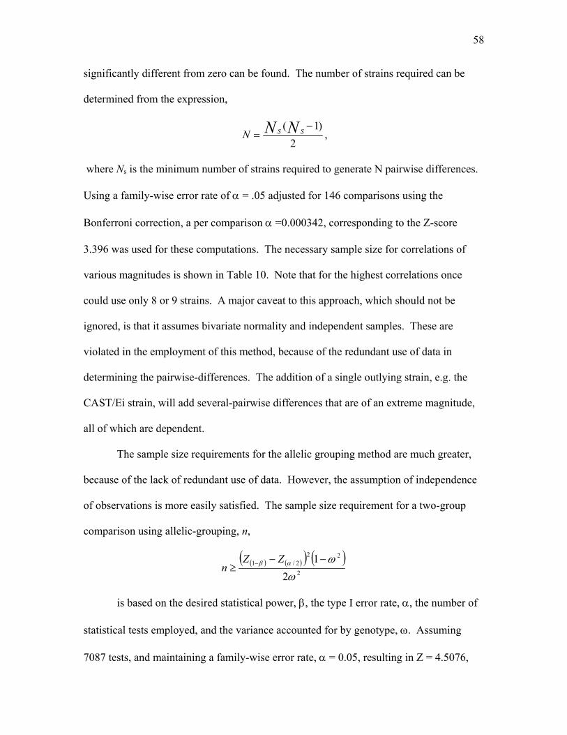
58

significantly different from zero can be found. The number of strains required can be

determined from the expression,

2)1( −

= NN SSN ,

where Ns is the minimum number of strains required to generate N pairwise differences.

Using a family-wise error rate of α = .05 adjusted for 146 comparisons using the

Bonferroni correction, a per comparison α =0.000342, corresponding to the Z-score

3.396 was used for these computations. The necessary sample size for correlations of

various magnitudes is shown in Table 10. Note that for the highest correlations once

could use only 8 or 9 strains. A major caveat to this approach, which should not be

ignored, is that it assumes bivariate normality and independent samples. These are

violated in the employment of this method, because of the redundant use of data in

determining the pairwise-differences. The addition of a single outlying strain, e.g. the

CAST/Ei strain, will add several-pairwise differences that are of an extreme magnitude,

all of which are dependent.

The sample size requirements for the allelic grouping method are much greater,

because of the lack of redundant use of data. However, the assumption of independence

of observations is more easily satisfied. The sample size requirement for a two-group

comparison using allelic-grouping, n,

( ) ( )( ) ( )2

222/1

21

ωωαβ −−

≥ − ZZn

is based on the desired statistical power, β, the type I error rate, α, the number of

statistical tests employed, and the variance accounted for by genotype, ω. Assuming

7087 tests, and maintaining a family-wise error rate, α = 0.05, resulting in Z = 4.5076,

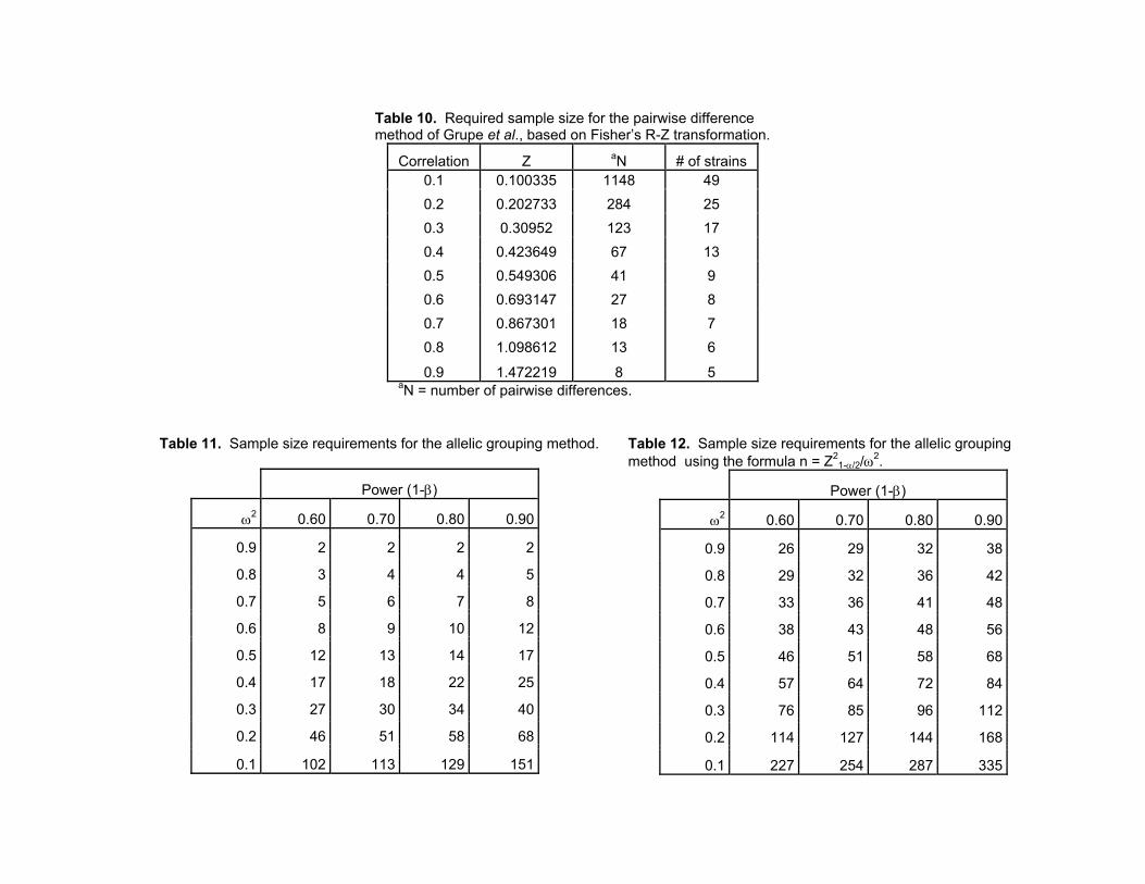
Table 10. Required sample size for the pairwise difference method of Grupe et al., based on Fisher’s R-Z transformation.

Correlation Z aN # of strains 0.1 0.100335 1148 49 0.2 0.202733 284 25 0.3 0.30952 123 17 0.4 0.423649 67 13 0.5 0.549306 41 9 0.6 0.693147 27 8 0.7 0.867301 18 7 0.8 1.098612 13 6 0.9 1.472219 8 5

aN = number of pairwise differences.

Table 11. Sample size requirements for the allelic grouping method.

Power (1-β)

ω2 0.60 0.70 0.80 0.90

0.9 2 2 2 2

0.8 3 4 4 5

0.7 5 6 7 8

0.6 8 9 10 12

0.5 12 13 14 17

0.4 17 18 22 25

0.3 27 30 34 40

0.2 46 51 58 68

0.1 102 113 129 151

Table 12. Sample size requirements for the allelic grouping method using the formula n = Z2

1-α/2/ω2.

Power (1-β)

ω2 0.60 0.70 0.80 0.90

0.9 26 29 32 38

0.8 29 32 36 42

0.7 33 36 41 48

0.6 38 43 48 56

0.5 46 51 58 68

57 64 72 84

0.3 76 85 96 112

0.2 114 127 144 168

0.1 227 254 287 335

0.4

60

the number of strains needed in each group for various values of β and ω are in Table 11.

More strains are required for the majority of markers, in which typically three or more

groups are being compared. Darvasi (2001) estimated that inbred strain based analyses

would require far more strains using the formula n = Z21−α/2/ω2 as shown in Table 12.

3.3.4 Peak detection. Several methods of peak detection may be employed. Presently,

neither method has high statistical power for attaining significance thresholds for most

QTLs using a single-marker (allele-grouping) or single-interval (pairwise-difference)

analysis corrected to maintain a genome-wide error rate of 5%. Grupe et al. (2001)

considered the top 5 to 20% of obtained results as peaks. This is arbitrary but has the

dubious merit of identifying some number of QTLs, whereas other techniques of error

control can potentially identify no QTLs. As mentioned, the latter case has virtually no

probability of being true for a heritable quantitative trait. Permutation analysis applied to

QTL mapping by Churchill and Doerge (1994), in which the Type I error rate is

controlled based on empirically derived significance levels, rather than from a theoretical

distribution that may not be obtainable for the actual data. This non-parametric approach

to error control is particularly useful in situations where the theoretical distribution of the

test statistic is unknown or when assumptions of normality are seriously violated. For

this method, to control the Type I error rate at α, the value of the test statistic exceeded

by the top α% of permutation results is the significance threshold. This can be

implemented at each marker or interval, by first 'shuffling' the phenotypes, then

subjecting each 'shuffle' to the mapping algorithm, alleviating some of the bias due to

uneven statistical power at markers in the allelic grouping method, and correlation

61

constraint in the pairwise-differences method. For each shuffle, the best result obtained

across the genome can also be used to determine the genome wide significance threshold.

Peaks can be identified either as those locations where the genome wide threshold is

achieved (although this will be biased by the linkage of SDPs capable of generating

higher power) or as those locations in which a particular comparison-wise threshold is

exceeded. The comparison-wise threshold can be adjusted to control for the number of

comparisons tested. It may be appropriate to also shuffle genotypic results as is done for

permutation analysis of F2 crosses. However, these are not experimentally derived in the

present analysis, and many non-existent strain distribution patterns will be tested in such

a shuffle, thus extending the permutations beyond the possible results obtainable. The

necessary number of permutations required for calculation of a stable significance

threshold can also be determined. Because of the small number of phenotypes in the

analysis, it may be feasible to generate all possible results and determine the exact p-

values rather than shuffling randomly.

Bonferroni adjustments of the comparison-wise permutation threshold or use of a

genome-wise permutation threshold can control the family-wise error rate, thus reducing

the large number of false positives expected due to multiple testing. An alternative

method for dealing with the multiple testing problem and identifying significant results is

to control the false discovery rate (Benjamini and Hochberg, 1995). Controlling this

error rate is more powerful than using the Bonferroni correction, thus decreasing Type II

errors, and is the most relevant for the QTL mapping concern of reducing the

consequences false detection. This method can be applied to determination of

significance thresholds based on the permutation adjusted p-values. To control this error

62

rate, the p-values are sorted in ascending order, and all hypotheses are rejected for which

i is less than or equal to the maximum value of i satisfying the inequality

qmipi ≤

where pi is the ith sorted p-value, m is the total number of hypotheses being tested and q is

the false discovery rate desired. Note that this assumes independence of the tests, an

assumption that is violated here.

3.3.5 Smoothing. Smoothing may aid in the visual detection of peaks, though much

information can be lost in the process of smoothing, particularly when results are

combined across correlated statistical tests without regard to that correlation. However,

the graphical display of mapping results might provide insight and intuitive appeal to

some users of these methods. Grupe et al. (2001) achieved this smoothing prior to the

analysis by taking a measure of the 'amount of polymorphism' present in a region of

genome. As discussed previously, this may not be appropriate. Smoothing the results

after the analyses are performed may be a superior way of considering the results of the

many tests within a cM position of genome, or across small highly linked regions of

genome. This post-analysis smoothing could give a sense of the average association

between genotype and phenotype in a region. Such smoothing must be able to take into

account two problems: the unequal dispersion of markers, which, if not considered will

result in averages containing points that are increasingly unrelated as inter-marker

distance increases, and the presence of linked markers, which can increase the weight of

the result at the linked markers artificially. The former problem can be dealt with

through dispersion weighted smoothing, and the latter problem can be dealt with by either

63

weighting each SDP in a region equally, or by culling the marker database to remove

markers within a region that have the same SDPs. With these concerns in mind, it seems

preferable to consider each point individually, rather than pool results of the adjacent

marker statistical tests through smoothing schemes.

3.3.6 Evaluation. In order to evaluate the success of a mapping algorithm, a trait for

which there exists complementary inbred strain survey data and QTL mapping studies in

genetically diverse populations is required. Though the goal of this work is to develop a

mapping method suitable for the study of behavioral phenotypes, particularly those

pertaining to pain, it may not be desirable to evaluate the method using existing studies

because of the small number of studies employed to date and because of the relatively

low genetic diversity represented in these studies. One trait that has been extremely well

characterized in the mouse is body weight, with inbred strain phenotypic data available

from the mouse phenome project (The Jackson Laboratory, 2000) and QTL mapping

results from numerous line crosses (e. g. Brockman et al., 1996; Brockman et al., 2000;

Cheverud et al., 1996; Cheverud et al., 2001; Kirkpatrick et al., 1998; Moody et al.,

1999; Morris et al., 1999; Keightly et al., 1996; Rance et al., 1997; Vaughn et al., 1999),

including perhaps one of the most detailed mapping study ever undertaken (Cheverud et

al., 1996; Cheverud et al., 2001; Vaughn et al., 1999), with many QTLs identified for

each of many traits in a cross of the inbred selected lines LG/J and SM/J. However,

consideration of only a single cross is insufficient. One of the important issues in

evaluating in silico mapping is that it takes advantage of a high amount of genetic

polymorphism, and if this genetic diversity is not reflected in the comparison QTL

64

mapping studies, the rate of false positive results generated by in silico mapping may be

grossly over-estimated.

The statistical comparison of these two methods with each other and with

previous findings is a difficult matter. Ideally, each can be evaluated for their relative

success at mapping mouse body weight relative to previous F2 crosses using Fisher's

exact test or the chi-square approximation. However, each method generates very

different output and is based on differing numbers of statistical tests. It is not readily

apparent how to compare 7000+ single marker analyses, the overlapping intervals

computed in Grupe’s method and hypothetically infinitely dense genome-wide scans used

for interval mapping in the F2 cross. Using the QTL confidence intervals (CIs) from the

F2 cross QTL is one possibility, for which the estimation of false positives (QTLs outside

the CI), false negatives (no QTL present in the CI), and true positives (QTL inside the CI)

is trivial, but the estimation of true negatives is problematic. One method is to divide the

genome into some arbitrary number of intervals approximately the size of a typical QTL

CI, and determine whether or not a QTL is present in that interval for each method.

However, this method is somewhat problematic in that single marker results have 0.1 cM

resolution, but are linked to QTLs some unknown distance from the marker. The size of

the region around a single marker result that should be considered “positive” is a

subjective matter. Another method is to look at single-marker results for each algorithm

at the F2 cross QTL peak. This assumes presence of a single marker at the QTL location

or near it with sufficient polymorphism in the SNP and microsatellite strain sets, neither

of which contain the strains used in the comparison F2 cross, and furthermore is not a

faithful representation of Grupe's (2001) method. The latter approach also does not

65

include the high proportion of true negatives in the analysis, and is flawed in the

assumption that all and only QTLs found in the previous mapping studies work are true.

Localization of QTLs to the correct chromosome alone can assist in the selection of the

relevant consomic/congenic strains, and this criterion should also be considered. In

selecting evaluation criteria, it is imperative to consider how the method is likely to be

used in practice; that is to ask, “Would the output obtained lead the researcher to

correctly continue evaluation of a region of the genome containing a QTL based on the

data, with a minimum of wasted effort?” Many approaches to the comparison of these

methods may not address this. For example, in the event of single marker results lying

just outside a QTL confidence region, this false positive in the strictest sense would be of

little practical consequence, particularly when considering that the size of these regions is

often under-estimated and may be distorted by scaling of diverse studies to a single

marker map. In another example, when multiple adjacent results are identified as

exceeding thresholds, the outer results, which may also be false-positives, would again be

of little consequence because follow-up research would focus on more central regions of

the identified segment of the genome.

3.4 Methods for development and evaluation of a mapping application.

3.4.1 Source data. Genotypic data. Genotypic data was obtained from three

databases containing microsatellite polymorphisms between strains. Because the three

data sets had slightly different strains represented and each affords different resolution

because of the number of markers it contains as shown in Table 9 (Dietrich et al., 1994,

http://wwwgenome.wi.mit.edu/genome_data/mouse/mouse_index.html; Schalkwyk et al.,

66

1999; http://www.mpimg-berlin-dahlem.mpg.de/~rodent/bin/polymarkerleo.cgi; Center

for Inherited Disease Research, http://www.cidr.jhmi.edu/mouse/mouse.html). SNP data

was derived from two sources, Massachusetts Institute of Technology (Lindblad-Toh et

al., 2000; http://waldo.wi.mit.edu/SNP/mouse/) and Roche Pharmaceuticals (Grupe et al.,

2001; http://mousesnp.roche.com/cgi-bin/msnp.pl). These databases have been merged

and are freely available in a single flat-file format (Williams, 2001;

http://www.nervenet.org/main/dictionary.html).

The data included in these analyses need not come from a single source, or be of a

particular marker type. However, the positions of markers are often relative to others in

the same set, and vastly uneven statistical power results from the different databases

rendering peak detection more difficult in combined datasets with vastly different sample

sizes. Thus, the databases will be considered separately from the one another for some

purposes.

Phenotypic data. Individual strain weights have been determined by The Jackson

Laboratory (Bar Harbor, ME) for a large number (n=40) of mice of each of several strains

(Table 9), all fed the same diet. These data were obtained from the Mouse Phenome

Database (The Jackson Laboratory, 2000). Body-weight and growth related phenotypes

are available for mice aged 3 weeks through 9 weeks. The majority of the evaluation was

performed for body weight at week 6, a trait that has been mapped in several different

and genetically diverse crosses

3.4.2 Model implementation. The models under consideration at the present time are the

allele grouping approach, in which strains are grouped by marker allele at each marker,

and the pairwise-difference approach in which the amount of polymorphism in a region

67

of genome is correlated with the amount of phenotypic difference. For the allele

grouping method, the linear model

y bik i ik= + +µ e

was fit for each marker using SAS (v. 8.2, The SAS Institute, Cary, NC) where the

phenotype strain mean yik for the kth strain of the ith allele class, as a mean value plus an

allele effect, bi, and a residual error eik,

The p-values resulting from each of these analyses were plotted against the

centiMorgan (cM) position of each marker. It should be noted that the actual location of

some of these markers is not agreed upon in the three microsatellite databases, nor are the

allele polymorphism groupings for some microsatellite markers. However, rather than

decide which markers were most accurately typed and placed, these redundant markers

were all included in the analysis. The resulting genotypic data set includes 7,087

markers, although it is anticipated that some of these markers will be unusable because of

missing marker data for strains with known phenotype, markers localized to a

chromosome, but not to a specific position, and a lack of sufficient correspondence of

allele polymorphism distribution with strain survey data such that modeling results are

defined.

The pairwise-difference algorithm described by Grupe et al. (2001) was also

implemented in SAS (v 8.2 The SAS Institute, Cary NC) making use of the full set of

SNPs and performing the permutation analysis. A Microsoft Excel implementation is

freely available from www.nervenet.org/xlfiles/SNP/CheslerSNPMapper.xls with the

CAST/Ei strain omitted from the analysis. Briefly, absolute phenotypic differences are

68

calculated for each possible pairing of strains. Genotypic differences are scored 1 for

same and 0 for different at each locus. These differences are summed within 30 cM

regions of genome, with each interval starting every 10 cM apart. The absolute

phenotypic differences, P, with elements pi, are correlated with the interval sum of

genotypic differences at each locus, GL , with elements gi, as follows:

rp g

p gPG

ii

n

iL

ii

n

iL

i

nL

2 1

1

2

1

2

=− −

−

−

=

= =

∑

∑ ∑

( )( )

( ) ( )

P G

P G

where

∑=

=n

i

i

ng

1

LGand P ==

∑ pn

i

i

n

1

are the means of the elements of the vectors of phenotypic difference and

genotypic difference at each locus (Grupe et al., 2001). These correlations are

standardized and plotted for each interval.

Permutation analysis was performed in SAS IML for both mapping methods.

Missing observations were first removed from the phenotype vector, and genotypes for

which no phenotype was present were also vetted. Missing values in the genotypic

marker databases remained. The phenotypes were then shuffled using ranked pseudo-

random numbers. The best p-value obtained for each marker database was retained to

establish genome-wise significance levels, and a count of the total number of times the

observed p-value from the actual data exceeded the p-value for the shuffled phenotypes

was also maintained. Exact comparison-wise adjusted p-values were reported, and

thresholds for various genome-wise significance levels were also reported by marker

database. The number of permutations required to obtain stable p-values was roughly

69

estimated by running four independent sets each of various numbers of permutations.

The mean and standard error of the genome-wise permutation p-values was evaluated for

each quantity of permutations. Control of the false discovery rate was also performed, as

described above.

3.4.3 Defining the comparison QTLs for reliability analysis. Many studies of body

weight and related phenotypes have been performed in a diverse group of mouse strains

and using a variety of methods for mapping and reporting. Studies were identified using

both a PubMed search for ‘[body weight or obesity] and QTL’ and a search of the Mouse

Genome Database (Blake et al., 2001) for QTLs for the phenotype “All-Growth/Weight

Abnormality: Postnatal”. Unfortunately, curation of the latter database is still in

progress and only QTLs on chromosomes 1 through 9 are accessible through this query.

Further studies were identified through the works cited in these sources. All QTLs were

initially considered, and the pool was narrowed to the specific phenotype for which strain

survey data was available and for which the largest amount of genetic diversity in the

mapping study populations existed, body weight at week six. QTLs in these studies were

detected and reported using a variety of procedures, not all of which were directly

comparable. All published QTLs for body weight at week six are listed in Table 13.

Only a few of these exceed Lander and Kruglyak’s (1995) proposed thresholds for a

genome-wide scan. Thus, QTLs found by genome-wise or chromosome-wise

permutations and other methods were often reported. Because each of these studies

generates a unique marker map based on observed recombinations, all QTLs were scaled

to the MIT map of the mouse genome (Dietrich et al. 1994). The relative location of the

Table 13. All published body weight QTLs for six week old mice QTL symbol Sexa Chrm

Significance Levelb

QTL Position

Lower CI

Upper CI

Position Scaledc

Lower CI scaledd

Upper CI scaled

Progenitors Reference

B 1 0.01ch 16.50 N/A N/A 7.70 centromere 17.70 Lg/J Sm/J Cheverud et al. (1996) Genetics 142:1305-1319. B 1 0.10 14.00 N/A N/A 14.00 4.00 24.00 DU6i DUK Brockman et al. (1998) Genetics 150:369-81.

Wt6q1 B 1 0.10lk 27.00 15 40 18.71 9.90 28.25 selected selected Moody et al. (1999) Genetics, 152:699-711. B 1 0.05lk 44.8 N/A N/A 32.04 22.04 42.04 Lg/J Sm/J Cheverud et al. (1996) Genetics 142:1305-1319.

Bw5 B 1 0.01 36.00 25 51 35.95 23.95 52.32 DU6i DBA/2OlaHsd Brockman et al. (2000) Genome Research 10:1941-1957. B 1 84.00 N/A N/A 63.50 53.50 73.50 Lg/J Sm/J Vaughn et al. (1999) Genetical Research 74:313-322. B 1 76.00 46 84 72.63 43.95 80.27 selected selected Keightly et al. (1996) Genetics 142:227-235. B 1 0.05 56.40 48.88 63.92 73.20 61.40 85.00 C57BL6/J DBA/2J Morris et al. (1999) Mammalian Genome 10:225-228.

Wt6q2 B 1 0.01lk 108.00 90 123 92.33 80.81 101.92 selected selected Moody et al. (1999) Genetics, 152:699-711. B 1 0.05lk 120.10 N/A N/A 99.50 89.50 109.50 Lg/J Sm/J Cheverud et al. (1996) Genetics 142:1305-1319.

B 2 0.10 56.00 N/A N/A 56.00 46.00 66.00 DU6i DUK Brockman et al. (1998) Genetics 150:369-81.

B 3 0.05ch 43.00 N/A N/A 27.50 17.50 37.50 Lg/J Sm/J Cheverud et al. (1996) Genetics 142:1305-1319.

B 4 0.05lk 32.10 N/A N/A 26.03 16.03 36.03 Lg/J Sm/J Cheverud et al. (1996) Genetics 142:1305-1319. B 4 50.00 N/A N/A 32.00 22.00 42.00 Lg/J Sm/J Vaughn et al. (1999) Genetical Research 74:313-322.. B 4 26.00 24 30 35.71 33.12 40.89 selected selected Keightly et al. (1996) Genetics 142:227-235. B 4 0.10 55.00 N/A N/A 55.00 45.00 65.00 DU6i DUK Brockman et al. (1998) Genetics 150:369-81.

Bw7 B 4 0.10 59.00 34 72 57.63 17.36 78.56 DU6i DBA/2OlaHsd Brockman et al. (2000) Genome Research 10:1941-1957. B 4 0.10lk 49.00 34 64 62.51 50.47 95.00 QS C57BL/6J Kirkpatrick et al. (1998) Mammalian Genome 9:97-102.

B 5 35.00 22 45 14.91 2.40 24.53 selected selected Keightly et al. (1996) Genetics 142:227-235. B 5 0.10 42.00 N/A N/A 42.00 32.00 52.00 DU6i DUK Brockman et al. (1998) Genetics 150:369-81.B 5 60.00 57 64 52.90 52.67 53.21 selected selected Keightly et al. (1996) Genetics 142:227-235.

Bw13 B 5 0.01 81.00 73 89 66.70 61.28 72.12 DU6i DBA/2OlaHsd Brockman et al. (2000) Genome Research 10:1941-1957.

B 6 22.00 15 26 11.33 4.43 15.27 selected selected Keightly et al. (1996) Genetics 142:227-235. B 6 0.05 70.50 57.0 telomere 51.04 40.44 61.64 C57BL6/J DBA/2J Morris et al. (1999) Mammalian Genome 10:225-228.

Continued on next page.

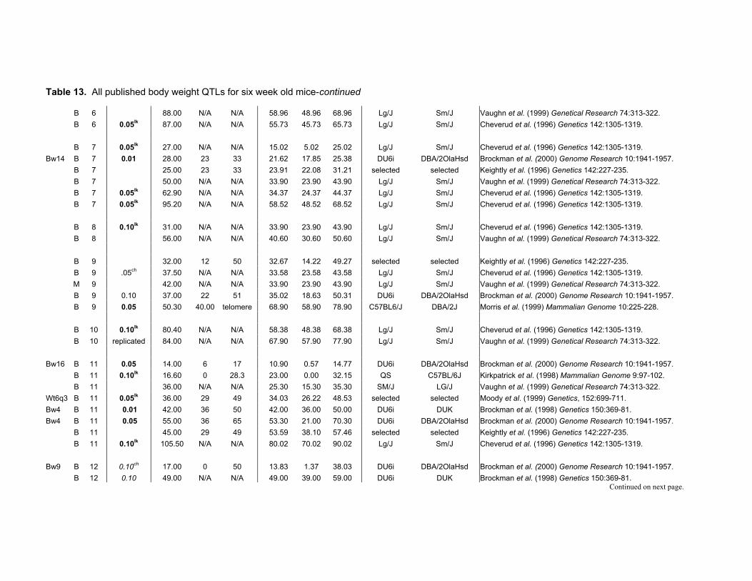
Table 13. All published body weight QTLs for six week old mice-continued B 6 88.00 N/A N/A 58.96 48.96 68.96 Lg/J Sm/J Vaughn et al. (1999) Genetical Research 74:313-322. B 6 0.05lk 87.00 N/A N/A 55.73 45.73 65.73 Lg/J Sm/J Cheverud et al. (1996) Genetics 142:1305-1319. B 7 0.05lk 27.00 N/A N/A 15.02 5.02 25.02 Lg/J Sm/J Cheverud et al. (1996) Genetics 142:1305-1319. Bw14 B 7 0.01 28.00 23 33 21.62 17.85 25.38 DU6i DBA/2OlaHsd Brockman et al. (2000) Genome Research 10:1941-1957. B 7 25.00 23 33 23.91 22.08 31.21 selected selected Keightly et al. (1996) Genetics 142:227-235. B 7 50.00 N/A N/A 33.90 23.90 43.90 Lg/J Sm/J Vaughn et al. (1999) Genetical Research 74:313-322. B 7 0.05lk 62.90 N/A N/A 34.37 24.37 44.37 Lg/J Sm/J Cheverud et al. (1996) Genetics 142:1305-1319. B 7 0.05lk 95.20 N/A N/A 58.52 48.52 68.52 Lg/J Sm/J Cheverud et al. (1996) Genetics 142:1305-1319. B 8 0.10lk 31.00 N/A N/A 33.90 23.90 43.90 Lg/J Sm/J Cheverud et al. (1996) Genetics 142:1305-1319. B 8 56.00 N/A N/A 40.60 30.60 50.60 Lg/J Sm/J Vaughn et al. (1999) Genetical Research 74:313-322. B 9 32.00 12 50 32.67 14.22 49.27 selected selected Keightly et al. (1996) Genetics 142:227-235. B 9 .05ch 37.50 N/A N/A 33.58 23.58 43.58 Lg/J Sm/J Cheverud et al. (1996) Genetics 142:1305-1319. M 9 42.00 N/A N/A 33.90 23.90 43.90 Lg/J Sm/J Vaughn et al. (1999) Genetical Research 74:313-322. B 9 0.10 37.00 22 51 35.02 18.63 50.31 DU6i DBA/2OlaHsd Brockman et al. (2000) Genome Research 10:1941-1957. B 9 0.05 50.30 40.00 telomere 68.90 58.90 78.90 C57BL6/J DBA/2J Morris et al. (1999) Mammalian Genome 10:225-228. B 10 0.10lk 80.40 N/A N/A 58.38 48.38 68.38 Lg/J Sm/J Cheverud et al. (1996) Genetics 142:1305-1319. B 10 replicated 84.00 N/A N/A 67.90 57.90 77.90 Lg/J Sm/J Vaughn et al. (1999) Genetical Research 74:313-322. Bw16 B 11 0.05 14.00 6 17 10.90 0.57 14.77 DU6i DBA/2OlaHsd Brockman et al. (2000) Genome Research 10:1941-1957. B 11 0.10lk 16.60 0 28.3 23.00 0.00 32.15 QS C57BL/6J Kirkpatrick et al. (1998) Mammalian Genome 9:97-102. B 11 36.00 N/A N/A 25.30 15.30 35.30 SM/J LG/J Vaughn et al. (1999) Genetical Research 74:313-322. Wt6q3 B 11 0.05lk 36.00 29 49 34.03 26.22 48.53 selected selected Moody et al. (1999) Genetics, 152:699-711. Bw4 B 11 0.01 42.00 36 50 42.00 36.00 50.00 DU6i DUK Brockman et al. (1998) Genetics 150:369-81.Bw4 B 11 0.05 55.00 36 65 53.30 21.00 70.30 DU6i DBA/2OlaHsd Brockman et al. (2000) Genome Research 10:1941-1957. B 11 45.00 29 49 53.59 38.10 57.46 selected selected Keightly et al. (1996) Genetics 142:227-235. B 11 0.10lk 105.50 N/A N/A 80.02 70.02 90.02 Lg/J Sm/J Cheverud et al. (1996) Genetics 142:1305-1319. Bw9 B 12 0.10ch 17.00 0 50 13.83 1.37 38.03 DU6i DBA/2OlaHsd Brockman et al. (2000) Genome Research 10:1941-1957. B 12 0.10 49.00 N/A N/A 49.00 39.00 59.00 DU6i DUK Brockman et al. (1998) Genetics 150:369-81.

Continued on next page.

Table 13. All published body weight QTLs for six week old mice-continued

Bw15 B 13 0.05 10.00 3 16 0.00 centromere 5.07 DU6i DBA/2OlaHsd Brockman et al. (2000) Genome Research 10:1941-1957. B 13 0.05ch 7.00 N/A N/A 1.10 centromere 11.10 Lg/J Sm/J Cheverud et al. (1996) Genetics 142:1305-1319. Bw10 B 13 0.01ch 47.00 33 61 33.15 20.23 46.08 DU6i DBA/2OlaHsd Brockman et al. (2000) Genome Research 10:1941-1957. B 13 0.05 34.00 N/A N/A 34.00 24.00 44.00 DU6i DUK Brockman et al. (1998) Genetics 150:369-81. B 13 86.00 N/A N/A 51.80 41.80 61.80 Lg/J Sm/J Vaughn et al. (1999) Genetical Research 74:313-322. B 13 59.00 29 telomere 56.93 29.93 telomere selected selected Keightly et al. (1996) Genetics 142:227-235. B 14 0.00 0 22 0.00 0.00 22.00 selected selected Keightly et al. (1996) Genetics 142:227-235. B 14 0.10lk 62.50 N/A N/A 32.28 22.28 42.28 Lg/J Sm/J Cheverud et al. (1996) Genetics 142:1305-1319. B 14 58.00 N/A N/A 46.10 36.10 56.10 Lg/J Sm/J Vaughn et al. (1999) Genetical Research 74:313-322. B 15 0.10 6.00 N/A N/A 6.00 centromere 16.00 DU6i DUK Brockman et al. (1998) Genetics 150:369-81. M 15 46.00 N/A N/A 39.90 29.90 49.90 Lg/J Sm/J Vaughn et al. (1999) Genetical Research 74:313-322. M 16 14.00 N/A N/A 17.50 7.50 27.50 Lg/J Sm/J Vaughn et al. (1999) Genetical Research 74:313-322. F 16 44.00 N/A N/A 47.50 37.50 57.50 Lg/J Sm/J Vaughn et al. (1999) Genetical Research 74:313-322. B 17 14.00 11 18 19.13 16.29 22.92 selected selected Keightly et al. (1996) Genetics 142:227-235. B X 0.05lk 23.00 18 28 18.83 17.08 30.45 selected selected Rance et al. (1997) Genetical Research 70:117-124. F X 0.10 42.00 N/A N/A 42.00 32.00 52.00 DU6i DUK Brockman et al. (1998) Genetics 150:369-81.

a. M=Male, F=Female, B=Both b. Significance levels were determined by genome-wise or chromosome-wise (denoted ‘ch’) permutation tests. In the event that LOD scores were reported, significance based on the criteria of Lander and Kruglyak for a genome-wide scan is denoted ‘lk’. c. Scaling was based on the marker position given by Dietrich et al. d. In the event that no confidence intervals were reported, a CI of ± 10 cM was used. Italicized significance thresholds indicate replicated QTL.

73

QTL to two known bracketing markers was determined from the marker map published

in the study by dividing the distance between the proximal marker and the QTL by the

difference between the proximal and distal marker position. The distance between

marker loci in the MIT database was then calculated, and the scaled QTL location was

determined by adding the relative distance to the proximal marker. Confidence intervals

were also inconsistently determined and reported, using 1-LOD or 2-LOD drop-offs. In

the event that confidence intervals were not reported but sufficient graphical results were

presented, the 1-LOD drop-off was determined from the graphs as measured with a

vernier caliper. In other studies, no confidence intervals were reported, and these were

arbitrarily assigned to be 10 cM up and downstream of the scaled QTL position.

3.4.4 Evaluation of models. The two mapping methods were each evaluated for

reliability. This was determined through counts of error rates of each model compared to

the previously published QTLs identified above using several criteria.

3.5 Results for the evaluation of haplotype based methods

3.5.1. Descriptive statistics for phenotypic data. Body weight data (Jackson Laboratory,

2000) is shown in Figure 5. At week six, the 16 inbred strains used in the present

analysis have a mean of 22.2, and standard deviation of 2.58. Weights ranged from 18.96

to 28.61. The trait is normally distributed (Shapiro-Wilks W = 0.897, p = 0.0725), and

thus satisfies model assumptions for the allelic-grouping approach. For the 8 strains for

which SNP data were available, a mean of 22.5 with a standard deviation of 2.87 was

observed. These body weights ranged from 19.45 to 28.61. This subset of the

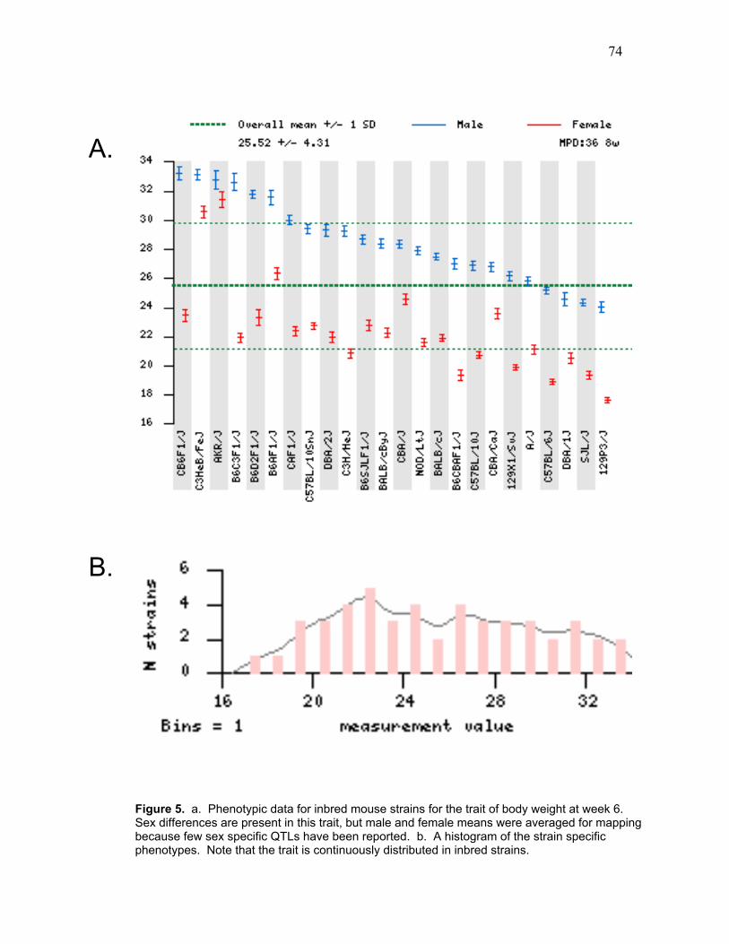
74

A.

B.

Figure 5. a. Phenotypic data for inbred mouse strains for the trait of body weight at week 6. Sex differences are present in this trait, but male and female means were averaged for mapping because few sex specific QTLs have been reported. b. A histogram of the strain specific phenotypes. Note that the trait is continuously distributed in inbred strains.

75

phenotypic data was also normally distributed (Shapiro-Wilks W = 0.875, p = 0.1694).

However, because the correlations are being run on the pairwise-differences, it is more

relevant to consider their distribution. The 28 pair-wise differences are non-normally

distributed (Shapiro-Wilks W = 0.892, p = 0.0076), with a mean of 3.19 and a median of

2.54 and a positively skewed distribution. The standard deviation is 2.55.

3.5.2 General mapping results. In the pair-wise differences method, 146 correlations

were run, with values ranging from -0.331 to 0.800. These correlations were not

normally distributed, W = 0.932, p < 0.0001, with a positive skew. The mean of this

distribution is 0.05530, with standard deviation 0.22. The median is 0.01279, and the

modal value is –0.05856. Four correlations appear to be strong outliers, over three

standard deviations from the mean, and an additional correlation is 2.5 standard

deviations from the mean. Pairwise-difference results are plotted in Figure 6.

In the allele grouping method, 5346 of the markers generated valid results. For

remaining tests, missing strains resulted in no variability in genotype for a particular

marker. At some markers, the variance accounted for by genotype was high, with ω2

estimates in excess of 0.90. These tests often had three or more levels of allele

represented, resulting in fewer than three strains in each group for the MIT markers.

Thus, the sample size was insufficient for statistically significant results based on

Bonferroni adjustments. Single-marker results for the allelic-grouping method are

plotted in Figure 7.

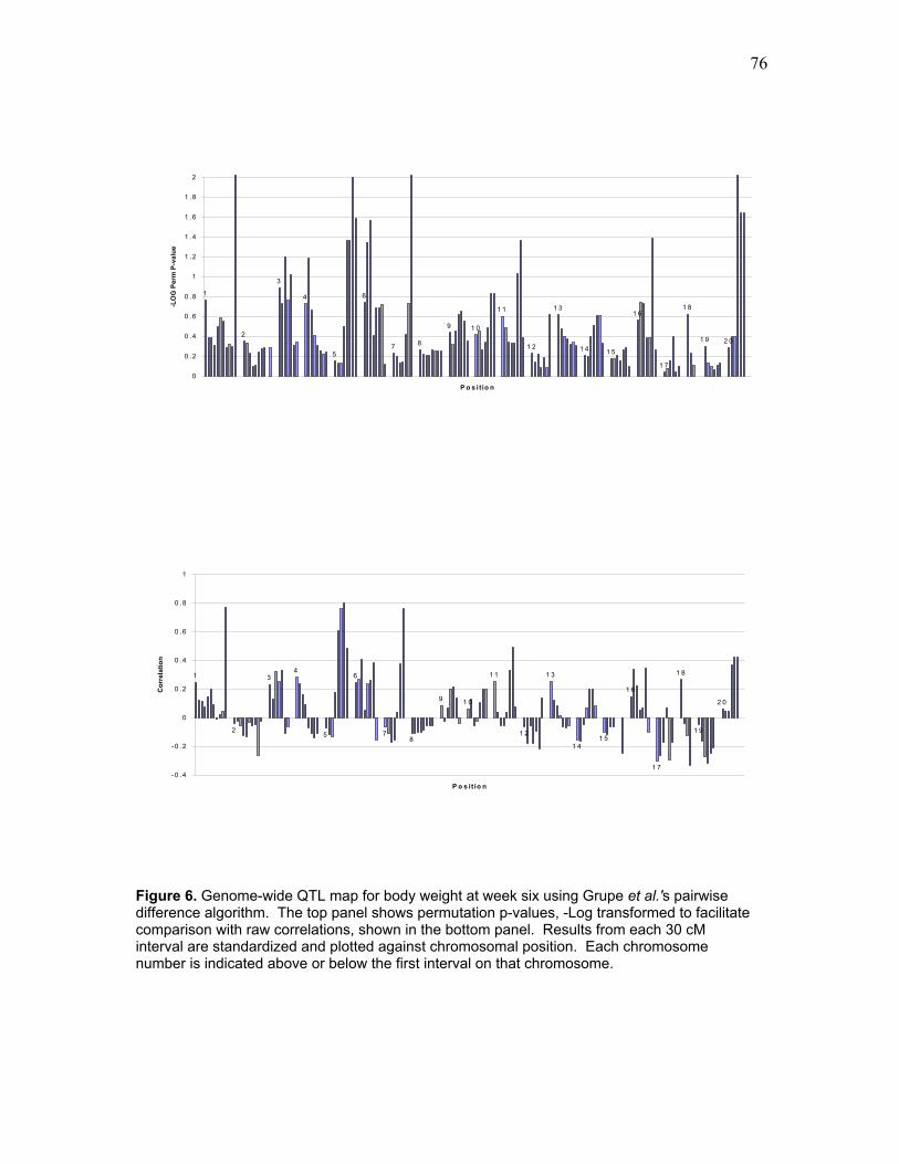
76

1

2

3

4

5

6

7 8

9 1 0

1 1

1 2

1 3

1 4 1 5

1 6

1 7

1 8

1 9 2 0

0

0 .2

0 .4

0 .6

0 .8

1

1 .2

1 .4

1 .6

1 .8

2

P o s i t io n

-LO

G P

erm

P-v

alue

Figure 6. Genome-wide QTL map for body weight at week six using Grupe et al.'s pairwise difference algorithm. The top panel shows permutation p-values, -Log transformed to facilitate comparison with raw correlations, shown in the bottom panel. Results from each 30 cM interval are standardized and plotted against chromosomal position. Each chromosome number is indicated above or below the first interval on that chromosome.

1

2

34

5

6

78

9 1 0

1 1

1 2

1 3

1 41 5

1 6

1 7

1 8

1 9

2 0

-0 .4

-0 .2

0

0 .2

0 .4

0 .6

0 .8

1

P o s it io n

Cor

rela

tion

77

Figure 7. Chromosome plots of allelic grouping results for body weight at week six. Each point is a single-marker result. The heavy black line is a seven-point moving average trend-line is imposed on each chromosome plot. Continued on next page.

C - 1

0

0 . 5

1

1. 5

2

2 . 5

3

3 . 5

4

4 . 5

0 2 0 4 0 6 0 8 0 10 0 12 0

cM Po s

C - 2

0

0.5

1

1.5

2

2.5

3

3.5

4

4.5

0 20 40 60 80 100 120

cM Po s

C - 3

0

0 . 5

1

1. 5

2

2 . 5

3

3 . 5

4

4 . 5

0 2 0 4 0 6 0 8 0 10 0 12 0

cM Po s

C - 4

0

0 . 5

1

1. 5

2

2 . 5

3

3 . 5

4

4 . 5

0 2 0 4 0 6 0 8 0 10 0 12 0

cM Po s

C - 5

0

0 . 5

1

1. 5

2

2 . 5

3

3 . 5

4

4 . 5

0 2 0 4 0 6 0 8 0 10 0 12 0

cM Po s

C - 6

0

0 . 5

1

1. 5

2

2 . 5

3

3 . 5

4

4 . 5

0 2 0 4 0 6 0 8 0 10 0 12 0

cM Po s

C - 7

0

0 . 5

1

1. 5

2

2 . 5

3

3 . 5

4

4 . 5

0 2 0 4 0 6 0 8 0 10 0 12 0

cM Po s

C - 8

0

0.5

1

1 .5

2

2 .5

3

3 .5

4

4 .5

0 20 40 60 80 100 12

cM Po s0

C - 9

0

0 . 5

1

1. 5

2

2 . 5

3

3 . 5

4

4 . 5

0 2 0 4 0 6 0 8 0 10 0 12 0

cM Po s

C - 10

0

0 . 5

1

1. 5

2

2 . 5

3

3 . 5

4

4 . 5

0 2 0 4 0 6 0 8 0 10 0 12 0

cM Po s

78

Figure 7. Chromosomse plots of allelic grouping results for body weight at week six-continued.

C - 11

0

0.5

1

1.5

2

2.5

3

3.5

4

4.5

0 20 40 60 80 100 120

c M P os

C- 12

0

0.5

1

1.5

2

2.5

3

3.5

4

4.5

0 20 40 60 80 100 120

c M P os

C - 13

0

0 . 5

1

1. 5

2

2 . 5

3

3 . 5

4

4 . 5

0 2 0 4 0 6 0 8 0 10 0 12 0

cM Pos

C - 14

0

0 . 5

1

1. 5

2

2 . 5

3

3 . 5

4

4 . 5

0 2 0 4 0 6 0 8 0 10 0 12 0

cM Pos

C - 15

0

0 . 5

1

1. 5

2

2 . 5

3

3 . 5

4

4 . 5

0 2 0 4 0 6 0 8 0 10 0 12 0

cM Pos

C - 16

0

0.5

1

1.5

2

2.5

3

3.5

4

4.5

0 20 40 60 80 100 120

cM Pos

C - 18

0

0 . 5

1

1. 5

2

2 . 5

3

3 . 5

4

4 . 5

0 2 0 4 0 6 0 8 0 10 0 12 0

cM Pos

C - 17

0

0.5

1

1.5

2

2.5

3

3.5

4

4.5

0 20 40 60 80 100 120

cM Po s

C - 19

0

0 . 5

1

1. 5

2

2 . 5

3

3 . 5

4

4 . 5

0 2 0 4 0 6 0 8 0 10 0 12 0

cM Pos

C - X

0

0 . 5

1

1. 5

2

2 . 5

3

3 . 5

4

4 . 5

0 2 0 4 0 6 0 8 0 10 0 12 0

cM Pos

79

3.5.3 Determining the number of permutations required The number of permutations

required to obtain stable adjusted p-values was determined by running independent sets

of 500, 1000, and 5000 permutations of the pair-wise difference method, and 500 and

1000 permutations of the allelic grouping method. The experiment-wise permutations

were stable to four decimal places at 1000 permutations of the allelic grouping method

and three decimal places at 5000 permutations by the pair-wise difference method based

on the standard errors observed from four independent runs for each permutation number.

3.5.4 Defined true positive QTLs. The complete list of previously published QTLs for

bodyweight at week six is given in Table 13. From this table, true positives were

identified based on scaled positions of the QTLs. These results from previous studies

were combined at various significance thresholds and listed in Table 14. The true

positive QTLs at several significance levels are also plotted in the first column of each

chromosome in Figure 8. Because eight genome-wide studies were combined, only the

0.01 per-study criterion controls the Type I error rate at less than 10%. However, several

studies did not distinguish between results exceeding the 0.05 and 0.01 experiment-wide

thresholds. Furthermore, some QTLs were merely reported as replications, regardless of

whether the replication was of a weak result exceeding chromosome-wise thresholds or a

“highly significant” QTL exceeding stringent genome-wise thresholds. The amount of

genome covered at each significance threshold was determined. If all reported QTLs

were considered, 60% of the genome is a true positive result. Thus, any result found by

in silico mapping would have a 60% chance of being confirmatory of previous findings.

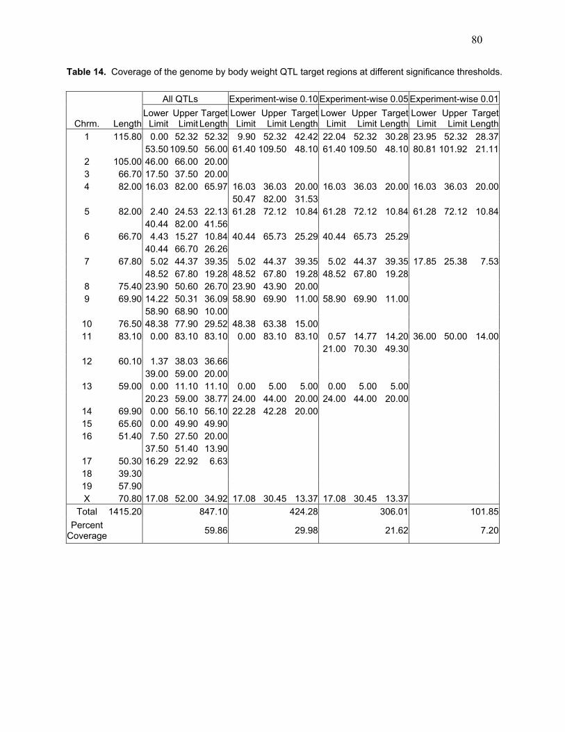
80

Table 14. Coverage of the genome by body weight QTL target regions at different significance thresholds.

All QTLs Experiment-wise 0.10 Experiment-wise 0.05 Experiment-wise 0.01

Chrm. Length Lower

Limit Upper

Limit Target Length

Lower Limit

Upper Limit

Target Length

Lower Limit

Upper Limit

Target Length

Lower Limit

Upper Limit

Target Length

1 115.80 0.00 52.32 52.32 9.90 52.32 42.42 22.04 52.32 30.28 23.95 52.32 28.37 53.50 109.50 56.00 61.40 109.50 48.10 61.40 109.50 48.10 80.81 101.92 21.112 105.00 46.00 66.00 20.00 3 66.70 17.50 37.50 20.00 4 82.00 16.03 82.00 65.97 16.03 36.03 20.00 16.03 36.03 20.00 16.03 36.03 20.00 50.47 82.00 31.53 5 82.00 2.40 24.53 22.13 61.28 72.12 10.84 61.28 72.12 10.84 61.28 72.12 10.84 40.44 82.00 41.56 6 66.70 4.43 15.27 10.84 40.44 65.73 25.29 40.44 65.73 25.29 40.44 66.70 26.26 7 67.80 5.02 44.37 39.35 5.02 44.37 39.35 5.02 44.37 39.35 17.85 25.38 7.53 48.52 67.80 19.28 48.52 67.80 19.28 48.52 67.80 19.28 8 75.40 23.90 50.60 26.70 23.90 43.90 20.00 9 69.90 14.22 50.31 36.09 58.90 69.90 11.00 58.90 69.90 11.00 58.90 68.90 10.00

10 76.50 48.38 77.90 29.52 48.38 63.38 15.00 11 83.10 0.00 83.10 83.10 0.00 83.10 83.10 0.57 14.77 14.20 36.00 50.00 14.00

21.00 70.30 49.30 12 60.10 1.37 38.03 36.66

39.00 59.00 20.00 13 59.00 0.00 11.10 11.10 0.00 5.00 5.00 0.00 5.00 5.00

20.23 59.00 38.77 24.00 44.00 20.00 24.00 44.00 20.00 14 69.90 0.00 56.10 56.10 22.28 42.28 20.00 15 65.60 0.00 49.90 49.90 16 51.40 7.50 27.50 20.00

37.50 51.40 13.90 17 50.30 16.29 22.92 6.63 18 39.30 19 57.90 X 70.80 17.08 52.00 34.92 17.08 30.45 13.37 17.08 30.45 13.37

Total 1415.20 847.10 424.28 306.01 101.85Percent

Coverage 59.86 29.98 21.62 7.20

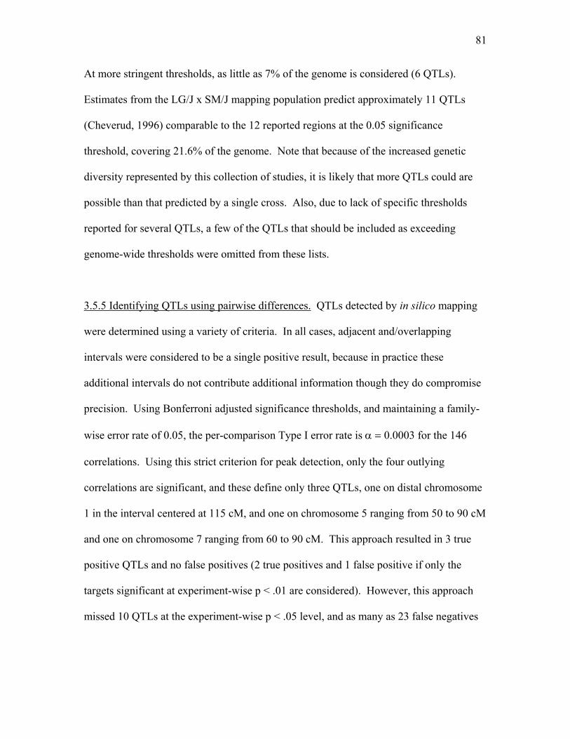
81

At more stringent thresholds, as little as 7% of the genome is considered (6 QTLs).

Estimates from the LG/J x SM/J mapping population predict approximately 11 QTLs

(Cheverud, 1996) comparable to the 12 reported regions at the 0.05 significance

threshold, covering 21.6% of the genome. Note that because of the increased genetic

diversity represented by this collection of studies, it is likely that more QTLs could are

possible than that predicted by a single cross. Also, due to lack of specific thresholds

reported for several QTLs, a few of the QTLs that should be included as exceeding

genome-wide thresholds were omitted from these lists.

3.5.5 Identifying QTLs using pairwise differences. QTLs detected by in silico mapping

were determined using a variety of criteria. In all cases, adjacent and/overlapping

intervals were considered to be a single positive result, because in practice these

additional intervals do not contribute additional information though they do compromise

precision. Using Bonferroni adjusted significance thresholds, and maintaining a family-

wise error rate of 0.05, the per-comparison Type I error rate is α = 0.0003 for the 146

correlations. Using this strict criterion for peak detection, only the four outlying

correlations are significant, and these define only three QTLs, one on distal chromosome

1 in the interval centered at 115 cM, and one on chromosome 5 ranging from 50 to 90 cM

and one on chromosome 7 ranging from 60 to 90 cM. This approach resulted in 3 true

positive QTLs and no false positives (2 true positives and 1 false positive if only the

targets significant at experiment-wise p < .01 are considered). However, this approach

missed 10 QTLs at the experiment-wise p < .05 level, and as many as 23 false negatives

82

Table 15. Best raw correlations for body weight week six using pairwise-differences.

Top 5% of Correlations Chromosome cM Raw Correlation Std. Correlation

1 115 0.77154 3.13462 5 55 0.60577 2.40913 5 65 0.76067 3.08703 5 75 0.80017 3.25992 5 85 0.48365 1.87467 7 75 0.75726 3.07213

11 75 0.49312 1.91612 X 55 0.42178 1.60391

5-10% Correlations

Chromosome cM Raw Correlation Std. Correlation6 35 0.40469 1.52912 6 75 0.38000 1.42107 7 65 0.37386 1.39417

16 25 0.33892 1.24128 16 65 0.34726 1.27777 X 45 0.36507 1.35569 X 65 0.42178 1.60391

10-15% Correlations

Chromosome cM Raw Correlation Std. Correlation3 35 0.32271 1.17031 3 55 0.33253 1.21332 4 15 0.28295 0.99632 6 25 0.26485 0.91712 6 65 0.26319 0.90982

11 65 0.33247 1.21304 13 15 0.25238 0.86251 18 15 0.2652 0.91865

15-20% Correlations

Chromosome cM Raw Correlation Std. Correlation1 15 0.24588 0.83409 3 15 0.23128 0.77020 3 45 0.25136 0.85806 4 25 0.23943 0.80585 6 15 0.24508 0.83060 6 55 0.23421 0.78302

11 15 0.25198 0.86077

83

occur when all QTLs from the literature are considered. Thus, potentially more powerful

approaches were considered.

For the pairwise differences algorithm, the top 5%, 10%, and 15% of standardized

correlations are listed in Table 15 as potential QTLs, as suggested in the original use of

the method (Grupe et al, 2001). This approach results in the identification of 5 distinct

peaks at the top 5% threshold. Though eight intervals are in the top 5%, several overlap,

and in practice would contribute no additional information. However, when compared to

targets significant at experiment-wise α = 0.01, only two of these are true positives, with

four false negatives. An additional two true positives are found in comparison to targets

significant at α = 0.05 and 0.1, with 9 and 12 false negatives respectively and all results

are true positives when considered against all known week six body-weight QTLs.

Using permutation analysis, reasonable experiment-wise significance thresholds

could not be met unless the Type I error rate was kept at 50%. However, due to the

uneven constraint on the correlations at each interval, a by comparison method of error

control might be more appropriate. The best peaks by permutation p-values are listed in

Table 16. Using Bonferroni adjustments to the significance threshold for comparison-

wise permutations, two peaks were again identified, both were true positives except in

comparison to the experiment-wise 0.01 targets. The error rates for various significance

thresholds are shown in Table 17, and graphically compared in Figure 8. Lowering the

threshold for comparison-wise permutation adjusted p-values to 0.01 resulted in the

detection of four true positives, two of which remain true positive in comparison to the

experiment-wise 0.01 targets. This resulted in no false positives when all targets,

experimentwise 0.1 targets or experimentwise 0.05 targets were considered, and two false

84

Table 16. Best permutation adjusted p-values for body weight at week six using pairwise-differences

Significant at Bonferroni adjusted threshold Chromosome cM Raw Correlation Std. Correlation Permutation P-Value

1 115 0.77154 3.13462 0.000 7 75 0.75726 3.07213 0.000

Significant at comparison-wise alpha = .01

Chromosome cM Raw Correlation Std. Correlation Permutation P-Value 5 75 0.80017 3.25992 0.010 X 45 0.36507 1.35569 0.005

Significant at comparison-wise alpha = .05

Chromosome cM Raw Correlation Std. Correlation Permutation P-Value 5 55 0.60577 2.40913 0.043 5 65 0.76067 3.08703 0.043 5 85 0.48365 1.87467 0.026 6 25 0.26485 0.91712 0.045 6 35 0.40469 1.52912 0.027

11 75 0.49312 1.91612 0.043 16 65 0.34726 1.27777 0.041 X 55 0.42178 1.60391 0.023 X 65 0.42178 1.60391 0.023

Significant at comparison-wise alpha = .15

Chromosome cM Raw Correlation Std. Correlation Permutation P-Value 3 15 0.23128 0.77020 0.129 3 35 0.32271 1.17031 0.063 3 55 0.33253 1.21332 0.095 4 25 0.23943 0.80585 0.065

10 65 0.19816 0.62522 0.149 10 75 0.19816 0.62522 0.149 11 65 0.33247 1.21304 0.094

Significant at comparison-wise alpha = .20

Chromosome cM Raw Correlation Std. Correlation Permutation P-Value 1 15 0.24588 0.83409 0.171 3 25 0.13206 0.33595 0.187 3 45 0.25136 0.85806 0.172 4 15 0.28295 0.99632 0.187 6 15 0.24508 0.83060 0.181 6 75 0.38000 1.42107 0.190 7 65 0.37386 1.39417 0.186

16 25 0.33892 1.24128 0.181 16 35 0.22464 0.74113 0.187

Table 17. Comparison of raw correlations and permutations for peak detection in the pairwise-differences method.

Previously Reported QTLs (Targets)

Raw Correlations

Permutations Previously Reported QTLs (Targets)

All 0.1 0.05 0.01 All 0.1 0.05 0.01 Bonferroni αfw=.05 TP 3 3 3 2 Bonferroni αfw=.05 TP 2 2 2 1

FP 0 0 0 1 FP 0 0 0 1 FN 23 13 10 4 FN 24 14 11 5

Top 5% TP 5 4 4 2 αcw = .01 TP 4 4 4 2 FP 0 1 1 3 FP 0 0 0 2 FN 21 12 9 4 FN 22 12 9 4

Top 10% TP 8 6 6 2 αcw = .05 TP 8 6 6 2 FP 0 2 2 6 FP 0 1 1 5 FN 18 9 7 4 FN 18 9 7 4

Top15% TP 11 8 8 4 αcw = .10 TP 10 7 7 4 FP 1 4 4 8 FP 0 2 2 6 FN 15 7 5 2 FN 16 8 6 2

Top 20% TP 12 9 10 5 αcw = .15 TP 11 8 7 4 FP 1 4 4 8 FP 0 2 3 6 FN 14 6 3 1 FN 15 7 6 2 αcw = .20 TP 13 9 8 5 FP 0 3 4 7 FN 13 6 5 1

86

positives when experiment-wise 0.01 targets were considered. Thus, permutation

adjusted p-values, even when controlled at the weak comparison-wise criteria of α = 0.05

generated more true positive results and fewer errors than the consideration of a quantile

of the best results. However, the rate of false negatives is still high, with approximately

half of the known QTLs missed at a threshold of α = 0.15. When the top 15% of results

are compared with the 15% permutation adjusted significance threshold, numbers of true

positives are similar, but again, permutations generate fewer false positive results.

However, even at this low threshold, many QTLs are missed. The control of the false

discovery rate as described by Benjamini and Hochberg (1995) should be more powerful

than strict Bonferroni correction, but this method is still rather strict. An FDR controlled

at 60% gives equivalent results to the 5% permutation threshold for this data.

3.5.6 Identifying QTLs using allelic grouping. Several different criteria for QTL

detection by the allelic grouping method were also examined. This was a bit problematic

because of the single-marker nature of the results. In keeping with the notion that these

methods should be evaluated with respect to the practical information they provide, it is

reasonable to question how far away from a single marker result one is willing to look for

a QTL. However, because virtually the entire genome is saturated with markers,

significant test results may be present at any point, though they may only be detectible

where haplotypes permit. Thus, for this analysis, results just outside a target region are

not considered true positives.

Bonferroni adjusted significance thresholds could not be met, either for

permutation adjusted or raw p-values. This is in part due to the large number of tests, but

87

even if only the most powerful analysis is considered (the 300 CIDR markers) no single

marker result reached this stringent threshold. Experiment-wise permutations were

problematic because of the small number of observations. With only 8 observations

being shuffled, and over six-thousand (though non-unique) strain distribution patterns

being tested, the same extreme p-value was reached in many of the genome-wide tests.

So, the Type I error rate could not be controlled at less than 20% for these markers using

this approach for the MIT markers. At this genome-wide threshold for MIT markers,

there were four true positives and one false positive when all targets were considered,

three true positives and two false positives when the experiment-wise 0.1 targets were

considered, and no true positives in comparison to the strictest sets of targets. None of

the markers in the Schalkwyk database reached the genome-wide threshold of 0.5, and

only four of the CIDR markers exceeded a permutation threshold of 0.5, with two true

positive results for all targets and experiment-wise 0.1 targets. Again, experiment-wise

permutations do not take into account the uneven statistical power at various markers,

and thus comparison-wise permutations were studied. The best peaks identified by

permutation-adjusted p-values are listed in Table 18. Using a comparison-wise

permutation adjusted α = 0.001, six peaks were discovered. Five of these were true

positives when compared to all targets, but only two of them were true positives when

compared to the experiment-wise 0.1 targets. None were true positives for higher

threshold targets. Considering a higher threshold, α = 0.01, 20 peaks were found. For all

targets there were 14 true positives and six false positives. For experiment-wise 0.1

targets, there were six true positives and 14 false positives. For experiment-wise 0.05

targets there were three true positives and 17 false positives. For experiment-wise 0.01

88

Table 18. Best single-marker results determined by permutation-adjusted p-value for the allele grouping method.

Comparison-wise alpha = 0.001 Locus Source Chrm cM P-value Perm P D2Mit399,D2Mit399.1,D2Mit399.2 MIT 2 60.1 7E-05 <.001 D2M148.1 CIDR 2 105 6E-04 0.001 D4Mit335 MIT 4 54.6 5E-04 <.001 D5Mit207 MIT 5 37.2 7E-05 <.001 D8Mit257 MIT 8 6.6 7E-05 <.001 D8Mit72 MIT 8 35 7E-05 <.001 D14M127.1 CIDR 14 10 2E-04 <.001

Comparison-wise alpha = 0.01 Locus Source Chrm cM P-value Perm P D1Mit279 MIT 1 25.1 0.119 0.008 D1Mit18 MIT 1 27.3 0.119 0.008 D1Mit478 MIT 1 28.4 0.119 0.008 D1Mit530 MIT 1 31.7 0.119 0.008 D1Mit176, D1Mit301 MIT 1 32.8 0.119 0.008 D1Mit510 MIT 1 113.7 5E-04 0.007 D2Mit303 MIT 2 50.3 6E-04 0.003 D3M67.1 CIDR 3 28 0.008 0.006 D3Mit124 MIT 3 40.4 0.119 0.008 D4Mit308 MIT 4 54.6 0.001 0.008 D5Mit276 MIT 5 37.2 0.119 0.008 D7M228.1 CIDR 7 18 0.005 0.008 D8Mit175 MIT 8 28.4 0.119 0.008 D8Mit27 MIT 8 35 3E-04 0.002 D8Mit262 MIT 8 38.3 0.119 0.008 D8Mit322 MIT 8 63.4 0.119 0.008 D9Mit244, D9Mit244.2 MIT 9 5.5 0.119 0.008 D9Mit350 MIT 9 60.1 5E-04 0.007 D10M96.1 CIDR 10 56 0.002 0.004 D11M285.1 CIDR 11 52 0.003 0.01 D11Mit58 MIT 11 60.1 0.004 0.008 D12Mit97 MIT 12 42.6 0.119 0.008 D16Mit131, D16Mit142 MIT 16 6.6 7E-04 0.008 D16Mit4 MIT 16 25.1 0.004 0.002 D17Mit116 MIT 17 20.8 0.096 0.007 D18Mit35 MIT 18 15.3 7E-04 0.008 D18Mit129 MIT 18 37.2 0.046 0.009 DXMit156 MIT X 56.8 0.096 0.008 DXM249.1 CIDR X 70.5 2E-04 0.002

0 5

101520253035

4045

50

55

60

65

70

75

80

8590 Column 1 Column 2 Column 3 Column 495

100 0.01 Known .001 AG Top 5% PD Comparisonwise Bonferroni PD105 0.05 Known .01 AG Top 10% PD Comparisonwise alpha=.01 PD

110 0.1 Known .025 AG Top 15% PD Comparisonwise alpha=.05 PD115 all .05 AG Top 20% PD Comparisonwise alpha=.15 PD

Comparisonwise alpha=.20 PD

X19181716151413121110987654321

Figure 8. In silico genome-wide scan for body weight QTLs summarized. Each chromosome is represented by 5 cM blocks and divided into four columns, with positions of known QTLs indicated in the first column (also shown in Table 14), allelic-grouping results in the second column (Table 17), pairwise-difference results using percent cut-offs as described by Grupe et al. (2001) in the third column (Table 15) and pairwise-difference results using empirical significance thresholds in the fourth column (Table16). True positive results are indicated by overlap of the in silico results (columns 2-4) with the results in the first column. For a single contiguous region, only a single positive or negative result was counted.

90

targets there was one true positive and 18 false positives. These error rates may be

artificially high because of the strict criteria that the marker had to be within the target

region. For one of several possible examples, a false positive result, D1Mit510, was at

113.7 cM on chromosome 1, only 4 cM away from the upper bound of the target. One

would not be misled in assuming a QTL on distal chromosome 1 based on the result.

However, definition of the size of the region around a single marker result can be very

arbitrary, and because numerous tests exist within the target interval, this was deemed

unnecessary. Control of the false discovery rate did perform better than the Bonferroni

adjustment, in that some results were identified as significant, as would be expected from

the increased power that this produces. However, error rates are still high, though there

were 4 true positive and 1 false positive results when compared to all targets, all results

were false positives when the experiment-wise .05 and .01 targets were considered. For

the experiment-wise 0.1 targets there were 3 false positives and two true positive results.

3.6 Discussion of early attempts at developing haplotype based QTL mapping

"In silico" haplotype-based QTL mapping can obtain some similarity to results of

F2 crosses. The technique appears to be capable of mapping with similar precision to

other techniques, though it currently requires enhancement of power, peak detection, and

error control. Empirically derived significance thresholds from permutation analysis

alleviate some of these concerns and improve error rates to acceptable levels. If these

problems can be resolved, this technique will be very beneficial to behavioral geneticists

because it can be employed rapidly, takes advantage of more polymorphic information,

and is amenable to the use of separate control groups. Furthermore, it makes use of data

91

that are typically collected on the way to later mapping studies and can be used to process

the growing body of phenomic data available for the mouse.

3.6.1 Comparison of the algorithms. The use of in silico mapping algorithms may prove

fruitful with enhancements of genotypic resources, but current resources and methods

provide insufficient statistical power for successful detection of many QTLs. A more

rigorous statistical approach to peak detection than that proposed by Grupe et al. (2001),

particularly the application of comparison-wise permutations, may enhance the quality of

mapping using the pairwise-difference method. This non-parametric method of

performing hypothesis testing performs better than simply considering the top

correlations, reducing the rate of false positives relative to the number of true positives.

The application of permutation tests addresses many of the criticisms of Grupe et al.’s

(2001) mapping method, particularly those concerns with bias due to constrained

correlations, the high rate of false positives and the use of arbitrary means of peak

detection. Without this or other enhancement to peak detection, the user will be faced

with an excessive amount of confirmatory research to do. The low resolution of the

approach still presents challenges in confirmation, and future efforts can investigate the

manipulation of the interval size and overlap on resolution. However, the method does

appear to correctly identify QTLs when stringent thresholds are applied, and the use of

consomic and overlapping congenic strains might allow further narrowing of the QTL

regions identified using this approach.

It was anticipated that allele grouping would work better than the pairwise-

difference algorithm, and that though the marker density is rather low, the larger amount

92

of strains in the CIDR database would provide more power and thus result in more

reliable mapping of the trait. Better performance was hypothesized for allele grouping

because the linear model employed is more appropriate for this method than it is for

pairwise-differences. However, the apparent statistical power of the pairwise-difference

method is higher due to the redundant use of phenotypes, and results of the allelic

grouping method were not as good as those of the pairwise-differences method.

This is in part because of insufficient sample sizes. The strategy of Grupe et al. (2001)

for boosting signal to noise ratios with the calculation of pairwise-differences appears to

be successful in this empirical evaluation.

3.6.2 Statistical approaches must be employed for peak detection. The present study

demonstrates that statistical issues must be considered in the determination of QTLs by in

silico mapping. The comment that “because in silico mapping is by definition an

artificial process, we used artificial methods to make our computational predictions

(Usuka et al, 2001)” does not excuse the high rate of false positives that can be generated

when one disregards a statistical approach to detection of positive results, and such an

approach can only reinforce the creditability issues facing the analysis of complex traits.

The consequence of retaining such a large number of positive results is an untenable

amount of follow up study, much of which will be fruitless. The arbitrary method of

identifying peaks of linkage generated 15 true positives, 11 false negatives and 24 false

positives in 10 comparisons reported by Grupe et al. (2001), in other words, 61% of the

follow up of QTLs identified by this method is likely to result in no QTL detection,

although due to concerns with a lack of genetic diversity in the comparison crosses, this

93

is likely to be an over-estimate of the error. Only those QTLs identified by statistical

criteria appear to replicate previous results with low error and thus a statistical approach

should be employed. Those QTLs retained after rigorously adjusting for multiple testing

are confirmatory of previously identified results, with an acceptably low rate of false

positives. More power can be obtained through the use of permutation tests run by

comparisons, while still controlling the rate of false positives. With additional strains

genotyped, this error rate can be improved. Another technique for statistical threshold

determination is the control of the relative frequency of false positives (Southey and

Fernando, 1998), which is somewhat difficult to implement because it requires a priori

hypotheses about QTL locations. However, if a database resource for genome-wide QTL

scans can be created, this information may be obtained from studies of related traits.

3.6.3 Evaluation issues. It should be noted that only a single trait was evaluated herein.

Evaluation issues may have affected the apparent success of these methods. The results

for allele grouping cover a much smaller portion of the genome than do the results for

pairwise differences, and the region surrounding each marker that would be considered

positive in practice needs to be incorporated into the evaluation. Thus, false negative

rates may be artificially low and false positive rates may be artificially high for the allele

grouping method. Figure 8 shows that there is potentially good reliability with allele

grouping that may not have been evident in this evaluation. In several cases where there

was no linkage observed across large portions of the genome, the allelic grouping method

and the pairwise difference method both successfully ruled out these regions, including

proximal chromosome 10, and chromosome 19.

94

Furthermore, the evaluation of these methods was based on a single comparison

phenotype, and ideally other traits should be used for evaluation of the method. Clearly

one should not optimize a method to replicate a single finding, running the risk of

developing an algorithm that performs poorly on other traits. An investigation of the

conditions under which this method works best would be quite useful, possibly

considering effects of heritability, phenotype distributions, and number of predicted

QTLs.

One reason for the disparity between this method and any single mapping study is

that computational methods employing a full panel of inbred strains are likely to detect

more QTLs than a single F2 cross. It has been shown the progenitor strains selected for a

cross can influence which QTLs are detected (Hitzemann et al., 2000). This is because

different crosses have different polymorphic information content at various regions.

Taking advantage of more genetic diversity will result in more QTL detection. Though

many of the strains employed in the present evaluation were selectively bred to be

extreme strains on body weight, and were derived from divergent sources (Beck et al,

2000), the genetic backgrounds represented in the in silico methods is different. The

increased genetic diversity represented in the strains used in allelic grouping may be in

part responsible for the disparate performance of this method.

3.6.4 Prospective evaluation is necessary. The difficulties encountered in the present

study with attempting meta-analysis of the existing literature and the caveat that the

strains used in the existing literature are not the strains employed in the in silico mapping

programs highlight the need for a thorough prospective evaluation of this method.

95

Ideally, a variety of crosses or an HS stock created from the genotyped strains should be

created and mapped with large sample sizes. The latter approach will be of considerably

more value because the marker map that is created will be on a single scale. The

proposed evaluation could be done under controlled experimental conditions so that the

phenotype observed is identical in both the inbred strain survey and the mapping study,

thereby reducing the impact of gene-environment interaction effects on QTL detection.

A major limitation of the present study is that body weight is assessed using diets with

varying fat contents, and genetic differences in weight gain following exposure to fatty

diets have been documented (e.g. West et al., 1994). Sex specific mapping should also be

employed if large sex differences in the trait exist. This was not done here because few

sex specific QTLs were found in the literature and thus weight data from the sexes were

pooled in the strain survey, though clearly, strain by sex effects are present in Figure 5.

3.6.5 Genetic resources need to be enhanced. In order to satisfy the demands for

increased statistical power, genotyping of SNPs or microsatellites of more strains should

continue. A higher density of SNPs can also afford greater precision to these methods,

and could potentially allow a single marker approach to be employed. Furthermore, if

strains are chosen with in silico mapping in mind, the quality of mapping could be

enhanced. Several of the present strains with known SNPs are highly similar, including

Balb/cJ and Balb/cbyJ, or A/J and A/HeJ.

Concerns with genetic origin effects can also be addressed by increasing the

number of genotyped strains. A major assumption in the present analysis is that markers

identical by state are indeed identical by descent. This applies to both SNP and

96

microsatellite based approaches because the SNPs are effectively used as markers when

considered across region, and because so many of the currently known SNPs are present

in “junk” DNA. Another assumption is that the QTLs are in a fixed relationship with the

markers. However, at some points in the generation of these inbred strains opportunities

for recombination arose, and thus similarity of markers does not necessarily mean

similarity of linked QTLs. This may be alleviated by incorporating some weighting by

the relatedness of strains either from radiation hybrid mapping or from the use of lineage

charts to develop a coefficient of relationship that can be included in these analyses. The

more precise determination of these values from breeding records is on the horizon (Beck

et al., 2000). The large number of strains in the CIDR database may provide sufficient

statistical power to evaluate the utility of incorporating genetic origin information;

however, phenotypic data is not available for all the strains in this database for the trait to

be considered (Table 9). Most of the commonly employed inbred strains are from either

Swiss-derived or Castle-Lathrop stock, although a further complication with this analysis

is that several strains are of isolated or unknown origin (Beck et al., 2001).

A major concern with in silico mapping is the accuracy and precision of the

positional information in the genotypic data. The MIT database used was created using

very few assays, has a lot of missing information, and has positional information which

has on more than one occasion been demonstrated to be inaccurate. Typically, in

performing QTL mapping, a high sample-size determination of marker position based on

the cross genotypes is performed to establish more accurately the marker locations. In

order for viable computational mapping to be performed, the accuracy of databased

97

genotypic data must be enhanced. This is in progress, and as genome assemblies are

completed, the exact locations of marker DNA will be known.

3.6.6 The need for realistic QTL reporting standards. Major difficulties in performing

meta-analysis of previously reported QTLs were encountered in the present study.

Though reporting guidelines have been made (e.g. Lander and Kruglyak, 1995) these are

considered too stringent and are not often employed in practice. To date, no consensus

exists on the reporting of QTLs, and the lack of confirmation of genetic polymorphisms

underlying QTLs has made publication of QTL studies difficult, leading to a file-drawer

problem. Reporting standards are essential for the combination of QTL data for

emerging methods, including evaluation of sub-phenotypes, and for evaluation of novel

mapping methods such as the one attempted here.

3.6.7 The need to employ multiple strains in QTL mapping studies. The present study

illustrates the need to consider multiple crosses in the identification of QTLs. Those

identified in a single study only explain polymorphism in a limited population. However,

using multiple crosses, far more QTLs are identified (Hitzemann et al. 2000). The

ultimate goal of QTL mapping is to identify the sources of genetic variability underlying

a trait. While a single cross may lead to a limited number of QTLs, many important

genetic factors can be missed, rendering the analysis of the trait incomplete.

3.6.8 Future directions for in silico mapping. Though only two major approaches to

mapping were compared here, many variations and combinations of approaches to in

98

silico methods are possible. In particular, use of the pair-wise difference method is not

necessarily restricted to the SNP database, and allele grouping is not restricted to the

microsatellites. Furthermore, the pre-analysis smoothing of the SNP database need not

be performed to implement the pair-wise difference algorithm, nor must the use of such

smoothing be restricted to this method and database.

Once a satisfactory model has been developed and validated through comparison

to existing mapping methods, its application to pain related phenotypes could commence.

Pain-related phenotypes for which QTLs have been identified and for which strain survey

data exist include morphine analgesia (Kest et al., 1999), and formalin pain sensitivity

(Wilson et al., 2002). Although the pairwise difference approach emerged as superior in

this analysis based on its better ability to detect previously reported QTLs, the allelic

grouping approach has some theoretical advantages that may make further study fruitful.

In particular, it is feasible to fit more complex models including interaction effects or

multiple trait models using an allelic grouping approach.

Though it requires substantially more power, a potential application of the allelic

grouping method of "in silico" mapping is for the identification of genes responsible for

individual differences in all of the phenotypes in a group of correlated traits. Not only

have pain related phenotypes been determined to be heritable; study of the genetic

correlation between these traits indicates common genetic mediation. We now know that

there are categories of related pain phenotypes that cluster based on stimulus category.

The thermal pain traits appear to have a common mediation, as do the

chemical/inflammatory (Mogil et al., 1999b). For analgesia, a number of different drug

classes appear to show surprisingly high genetic correlation, implying the existence of

99

“master analgesia genes” (Wilson et al., 2002). Such genes may play a role in the general

phenomena of pain and analgesia, unrestricted to a single modality or neurochemical

system. Several categories of pain have been identified (Mogil et al., 1999b) through

multidimensional scaling (MDS), and these traits may be mapped simultaneously to

identify genes underlying sensitivity to correlated traits. Though multiple trait mapping

is possible from F2 crosses, “in silico” techniques offer a tremendous advantage in that

they can be used to perform analyses in which multiple measures are taken in separate

though genetically homogenous individuals. Thus, concerns typical to behavioral

experiments such as carry-over effects from repeated testing can be eliminated. Further,

strain means are far more precise estimates of trait values than individual observations.

Strain-specific environmental effects are an example of traits that require multiple

measures in different testing contexts, and that while clearly of consequence, are not

established sufficiently to generate interest in an experimental cross. The magnitude of

sex differences, experimenter induced effects, and sensitivity to effects of within-cage

testing order, crowding, circadian factors, humidity and seasonal effects have been shown

above to differ between strains. Strain differences in sensitivity to the environment may

be traits that are conducive to genetic mapping. They can ultimately be used for

identification of the genes that underlie the influence of these environmental factors on

sensitivity to pain. Essentially, this analysis can find genes that "transduce"

environmental influence into individual differences in behavior. Using estimated

environmental effects in the inbred mouse strains, mapping of the QTLs that underlie

susceptibility of the trait to these environmental factors can be performed in silico. Some

of the neurochemical substrates have been identified for these environmental influences

100

on behavior, and could be the source of individual differences in their effects. For

example Daniels et al. (2000), has shown that overcrowding is anxiety provoking, and

results in a decreased number of serotonin 5HT-1 receptors in rats. Restraint stress has

been shown to alter neurotransmission for several biogenic amines, and

acetylcholinesterase activity (Sunanda, 2000). Based on these findings, one may predict

that genetic variation in 5HT-1 receptors may result in differential sensitivity to crowding

stress, and that differences in the identified aminergic systems may result in a differential

effect of restraint stress. Kavaliers and Hirst (1983) have shown that two different mouse

strains show different patterns of circadian effects, and this may be related to albinism.

Thus, one would predict that some association with coat color genes (or retinal

degeneration genes) might be present for this environmental influence.

101

4. Conclusion: Using Inbred Strains to Characterize Individual Differences

Though they have been viewed as a somewhat unsophisticated resource for

modern genetic analysis, the existing inbred strains can provide a wealth of information

for the understanding of individual differences because of their fixed genotypes and the

relationship that the strains share with one another. These mice are generally used to

identify heritability of traits, as specific disease models, as mutant background strains, or

as progenitors in genetic mapping studies. Because a large number of mice of identical

genotype can be tested in a variety of contexts the role of the gene-environment

interaction can also be investigated in these strains. The application of modern data-

mining methods to large-scale phenotyping projects can generate a wealth of information

about environmental effects on these traits, particular with regard to laboratory factors

that may impact results generated when data from multiple sites are considered together.

The role of the laboratory environment on the genetic study of complex traits, particularly

of behavior, can and should be defined. This is especially necessary as large-scale

projects such as the Mouse Phenome Project attempt to associate results from multiple

labs using phenotypic data from inbred strains, and the environmental data associated

with many of these phenotypes is available (Bogue, 2002).

Furthermore, the utility of these strains may be greatly enhanced as the advance

from the sequencing of their genomes to annotation and beyond is made. The data

generated in large-scale genomics projects has made possible the use of inbred strain

resources to understand the genetic basis of complex traits. Associating inbred strain

differences in genomic data with phenotypes is an emerging use of bio-informatics

resources, and enhancement of these ‘in silico’ trait-mapping methods can make them

102

reliable enough to be used in common practice. This can be especially beneficial in

enabling non-geneticists to take advantage of the power of genetic methods in the study

of complex traits. For the geneticist, these techniques can be used optimize selection of

progenitor strains for genetic crosses, reduce genotyping effort and expenditure, or, if

sufficiently enhanced, even lead to direct candidate gene testing from the inbred strain

survey, thereby completely eliminating the need for genotyping. However, it is hoped

that the development of tools to process genomic and phenotypic databases will allow a

wider variety of biologists to benefit from the results of genetic analysis.

Recently, emphasis has been placed on achieving medical research goals through

the use of genetic mouse models. A more thorough understanding of the genetic and

environmental influences occurring in these studies is required for promising application

of the results. Together, this work demonstrates two ways in which inbred strains can be

used in the characterization of individual differences in complex traits that have been or

can be applied to pain related phenotypes. The understanding gained from the study of

individual differences in pain is the first step toward development of bio-behavioral pain

therapies tailored to individuals suffering from a variety of pain conditions. However,

pain related phenotypes are but one example of the possible applications of these efforts.

103

5. References Adler, M. W., Mauron, C., Samanin R., and Valzelli L. (1975). Morphine analgesia in

grouped and isolated rats. Psychopharmacologia 41:11-14. Aikman, H. (1997). The association between arthritis and the weather. Int. J.

Biometeorol. 40:192 -199. Beck, J. A., Lloyd, S., Hafezparast, M., Lennon-Pierce, M., Eppig, J. T., Festing, M. F.,

and Fisher, E. M. (2000). Genealogies of mouse inbred strains. Nat Genet. 24:23-5.

Belknap, J. K., Hitzemann, R., Crabbe, J. C., Phillips, T. J., Buck, K. J., and Williams, R.

W. (2001). QTL analysis and genome-wide mutagenesis in mice: complementary genetic approaches to the dissection of complex traits. Behav Genet. 31:5-15.

Belknap, J. K., Mogil, J. S., Helms, M. L., Richards, S. P., O'Toole, L. A., Bergeson, S.

E., and Buck, K. J. (1995). Localization to chromosome 10 of a locus influencing morphine analgesia in crosses derived from C57BL/6 and DBA/2 strains. Life Sci. 57:117-124.

Ben-Bassat, J., Peretz, E., Sulman, F.G. (1959). Analgesimetry and ranking of analgesic

drugs by the receptacle method. Arch Int Pharmcodyn Ther. 122:434-447. Benjamini, Y., and Hochberg, Y. (1995). Controlling the false discovery rate: a practical

and powerful approach to multiple testing. J. R. Statist. Soc. B. 57:289-300. Bergeson, S. E., Helms, M. L., O'Toole, L. A., Jarvis, M. W., Hain, H. S., Mogil, J. S.,

Belknap, J. K. (2001). Quantitative trait loci influencing morphine antinociception in four mapping populations. Mamm Genome. 12:546-553.

Berkley, K. J. (1997). Sex Differences in Pain. Behav. Brain Sci. 20:371-380. Blake, J. A., Eppig, J. T., Richardson, J. E., Bult, C. J., Kadin, J. A., and the Mouse

Genome Database Group. (2001). The Mouse Genome Database (MGD): Integration Nexus for the Laboratory Mouse. Nucleic Acids Res. 29:91-94.

Bonnet, K. A., Hiller, J. M., and Simon, E. J. (1976). The effects of chronic opiate

treatment and social isolation on opiate receptors in the rodent brain. In Kosterlitz, H. W. (Ed.), Opiates and Endogenous Opioid Peptides. Elsevier/North Holland Press: Amsterdam.

Bogue, M. (2002). Inbred strains revitalized: sharpening a classical genetics tool to add to

the complex traits toolbox. Intl Complex Trait Consortium Meeting, 8.

104

Breiman, L., Friedman, J., Olshen, R., and Stone, C. (1984). Classification and Regression Trees. Wadsworth: Pacific Grove, CA.

Brockmann, G. A., Haley, C. S., Renne, U., Knott, S. A., and Schwerin, M. (1998).

Quantitative trait loci affecting body weight and fatness from a mouse line selected for extreme high growth. Genetics 150: 369-381.

Brockmann, G. A., Kratzsch, J., Haley, C. S., Renne, U., Schwerin, M., and Karle, S.

(2000). Genome Research 10:1941-1957. Cabib, S., Orsini, C., LeMoal, M., and Piazza, P. V. (2000). Abolition and reversal of

strain differences in behavioral responses to drugs of abuse after a brief experience. Science 289:463-465.

Castellano, C., Puglisi-Allegra, S., Renzi, P., and Oliverio, A. (1985). Genetic differences

in daily rhythms of pain sensitivity in mice. Pharmacol Biochem Behav. 23:91-92. Center for Inherited Disease Research (CIDR) Mouse Marker Set. (2001). World Wide

Web (URL: http://pages.cidr.nhgri.nih.gov/mouse/mmset.html). Chesler, E. J., Rodriguez-Zas, S. L., Mogil, J. S. (2001) In silico mapping of mouse

quantitative trait loci. Science 294:2423. Cheverud, J. M., Routman, E. J., Duarte, F. A. M., van Swinderen, B., Cothran, K. and

Perel, C. (1996). Quantitative trait loci for murine growth. Genetics 142:1305-1319.

Cheverud, J. M., Vaughn, T. T., Pletscher, L. S., Peripato, A. C., Adams, E. S., Erikson,

C. F., King-Ellison, K. J. (2001). Genetic architecture of adiposity in the cross of LG/J and SM/J inbred mice. Mamm Genome 12:3-12.

Churchill, G. A. and Doerge, R. W. (1994). Empirical threshold values for quantitative

trait mapping. Genetics 138: 963-971. Copeland, N. G., Gilbert, D. J., Jenkins, N. A., Nadeau, J. H., Eppig, J. T., Maltais, L. J.,

Miller, J. C., Dietrich, W. F., Steen, R. G., Lincoln, S. E., Weaver, A., Joyce, D. C., Merchant, M., Wessel, M., Katz, H., Stein, L. D., Reeve, M. P., Daly, M. J., Dredge, R. D., Marquis, A., Goodman, N., and Lander, E. S. (1993). Genome maps IV. Science 262:67-82.

Supplemented by additional markers in: Whitehead Institute/MIT Center for

Genome Research, Genetic Map of the Mouse, Database Release 10, April 28, 1995.

105

Coudereau, J. P., Monier, C., Bourre, J. M., and Frances, H. (1997). Effect of isolation on pain threshold and on different effects of morphine. Prog Neuropsychopharmacol Biol Psychiatry. 21: 997-1018.

Crabbe, J. C, Wahlsten, D., and Dudek, B.C. (1999). Genetics of mouse behavior:

Interactions with laboratory environment, Science 284, 1670-1672. Cunningham, D. J., Benson, W. M., and Hardy, J. D. (1957). Modification of the thermal

radiation method for assessing antinociceptive activity in the rat. J. Appl. Physiol. 11, 459-464.

D’Amour, F. E. and Smith, D. L. (1941). A method for determining the loss of pain

sensation, J. Pharmacol. Exp. Ther. 72, 74-79. Daniels, W. M., Pietersen, C. Y., Carstens, M. E., Daya, S., and Stein, D. (2000).

Overcrowding induces anxiety and causes loss of serotonin 5HT-1a receptors in rats. Metab Brain Dis. 15:287-95.

Darvasi, A.(2001) In Silico Mapping of Mouse Quantitative Trait Loci. Science, 294:

2423. Darvasi, A. and Soller, M. (1995) Advanced intercross lines, an experimental population

for fine genetic mapping. Genetics 141:1199-207 Darvasi, A., Weinreb, A., Minke, V., Weller, J. I., and Soller, M. (1993). Detecting

marker-QTL linkage and estimating QTL gene effect and map location using a saturated genetic map. Genetics 134:943-51.

Defeudis, F. V., Defeudis, P. A., and Somoza, E. (1976). Altered analgesic responses to

morphine in differentially housed mice. Psychopharmacology 49: 117-118. Dietrich, W. F., Miller, J. C., Steen, R. G., Merchant, M., Damron, D., Nahf, R., Gross,

A., Joyce, D. C., Wessel, M., Dredge, R. D., et al. (1994). A genetic map of the mouse with 4,006 simple sequence length polymorphisms. Nat Genet. 7:220-245.

Flaherty, L., and Bolivar, V. J. (2002). Mapping of genes influencing open field and fear

conditioning by use of knockout/congenic strains. Intl. Complex Trait Consortium Meeting, 16.

Folkard, S., Glynn, C. J., and Lloyd, J. W. (1976). Diurnal variation and individual

differences in the perception of intractable pain. J. Psychosom. Res. 20: 289-301 Frederickson, R. C., Burgis, V., Edwards, J. D. (1977). Hyperalgesia induced by

naloxone follows diurnal rhythm in responsivity to painful stimuli. Science 198: 756-758.

106

Gentsch, C., Lichtsteiner, M., Frischknecht, H. R., Feer, H., and Siegfried B. (1988). Isolation-induced locomotor hyperactivity and hypoalgesia in rats are prevented by handling and reversed by resocialization. Physiol. Behav. 43, 13-16.

Gora-Maslak, G., McClearn, G. E., Crabbe, J. C., Phillips, T. J., Belknap, J. K., and

Plomin R. (1991). Use of recombinant inbred strains to identify quantitative trait loci in psychopharmacology. Behav Genet. 21:99-116.

Grupe, A., Germer, S., Usuka, J., Aud, D., Belknap, J. K., Klein, R. F., Ahluwalia, M. K.,

Higuchi, R., and Peltz, G. (2001). In silico mapping of complex disease-related traits in mice. Science 292: 1915-1918.

Hain, H. S., Belknap, J. K., and Mogil, J. S. (1999). Pharmacogenetic evidence for the

involvement of 5-hydroxytryptamine (Serotonin)-1B receptors in the mediation of morphine antinociceptive sensitivity. J Pharmacol Exp Ther. 291:444-449.

Hawley, D. J., Wolfe, F., Lue, F. A., and Moldofsky, H. (2001). Seasonal symptom

severity in patients with rheumatic diseases: a study of 1,424 patients. J Rheumatol. 28:1900-1909.

Hayes, W. L. (1994) Statistics, 5th ed. Harcourt Brace: Fort Worth, TX. Hitezemann, R., Demarest, K., Koyner, J., Cipp, L., Patel, N., Rasmussen, E., and Mc

Caughran, J., Jr., (2000). Effect of genetic cross on the detection of quantitative trait loci and a novel approach to mapping QTL's. Pharmacol Biochem Behav. 67:767 – 772.

Jackson Laboratory (2000). Body weights for selected strains, by age, MPD:36. Mouse

Phenome Database Website, The Jackson Laboratory, Bar Harbor, Maine. World Wide Web (URL: http://www.jax.org/phenome). May, 2002.

Johnson, R.A. and Wichern, D.W. (1998) Applied Multivariate Statistical Analysis, 4th

ed. Prentice Hall: New Jersey. Jorum, E. (1988). Analgesia or hyperalgesia following stress correlates with emotional

behavior in rats. Pain 32:341-348. Kavaliers, M. and Hirst, M. (1983). Daily rhythms of analgesia in mice: effects of age

and photoperiod. Brain Res. 279:387-393. Keightley, P. D., Hardge, T., May, L., Bulfield, G. (1996). A genetic map of quantitative

trait loci for body weight in the mouse. Genetics. 142: 227-235. Kest, B., Wilson, S. G., Mogil, J. S. (1999). Sex differences in supraspinal morphine

analgesia are dependent on genotype. J Pharmacol Exp Ther. 289: 1370-1375.

107

Kirkpatrick, B. W., Mengelt, A., Schulman, N., Martin, I. C. A. (1998) Identification of quantitative trait loci for prolificacy and growth in mice. Mamm Genome 9: 97-102.

Kleitman, N. (1963). Sleep and Wakefulness. University of Chicago Press: Chicago, IL. Lander ES, Botstein D. (1989). Mapping mendelian factors underlying quantitative traits

using RFLP linkage maps. Genetics 121:185-99. Lander, E.S. and Kruglyak, L. (1995). Genetic dissection of complex traits: Guidelines

for interpreting and reporting linkage results. Nat Genetics 11:241-247. Lander, E. S. and Schork, N. J. (1994). Genetic dissection of complex traits. Science

265:2037-2048. Lariviere, W. R., Chesler, E. J., and Mogil, J. S. (2001). Transgenic studies of pain and

analgesia: mutation or background genotype? J Pharmacol Exp Ther. 297:467-73. Le Roy, I., Roubertoux, P. L., Jamot, L., Maarouf, F., Tordjman, S., Mortaud, S.,

Blanchard, C., Martin, B., Guillot, P. V., and Duquenne, V. (1998). Neuronal and behavioral differences between Mus musculus domesticus (C57BL/6JBy) and Mus musculus castaneus (CAST/Ei). Behav Brain Res. 5: 135-42.

Lindblad-Toh, K., Winchester, E., Daly, M. J., Wang, D. G., Hirschorn, J. N., Laviolette,

J-P., Ardlie, K., Reich, D. E., Robinson, E., Sklar, P., Shah, N., Thomas, D., Fan, J. B., Gingeras, T., Warrington, J., Patil, N., Hudson, T. J., and Lander, E. S. (2000). Large-scale discovery and genotyping of single-nucleotide polymorphisms in the mouse. Nat Genetics 24:381-386.

Lynch, M. and Walsh, B. (1998). Genetics and Analysis of Quantitative Traits. Sinauer:

Sunderland, MA. Loh, W-Y and Shih, Y-S. (1997). Split selection methods for classification trees.

Statistica Sinica 7:815-840. Mogil, J. S. (1999). The genetic mediation of individual differences in sensitivity to pain

and its inhibition. Proc Natl Acad Sci 96:7744-7751. Mogil, J. S., Chesler, E. J., Wilson, S. G., Juraska, J. M., and Sternberg, W. F. (2000).

Sex differences in thermal nociception and morphine antinociception in rodents depend on genotype. Neurosci Biobehav Rev 24:375-89.

Mogil, J. S., Richards, S. P., O'Toole, L. A., Helms, M. L., Mitchell, S. R., and Belknap,

J. K. (1997a). Genetic sensitivity to hot-plate nociception in DBA/2J and C57BL/6J inbred mouse strains: possible sex-specific mediation by delta2-opioid receptors. Pain 70:267-277.

108

Mogil, J. S., Richards, S. P., O'Toole, L. A., Helms, M. L., Mitchell, S. R., Kest, B., and

Belknap, J. K. (1997b). Identification of a sex-specific quantitative trait locus mediating nonopioid stress-induced analgesia in female mice. J Neurosci. 17:7995-8002.

Mogil, J. S., Wilson, S. G., Bon, K., Lee, S. E., Chung, K., Raber, P., Pieper, J. O., Hain,

H. S., Belknap, J. K., Hubert, L., Elmer, G. I., Chung, J. M., and Devore, M. (1999a). Heritability of nociception I: Responses of 11 inbred mouse strains on 12 measures of nociception. Pain 80:67-82.

Mogil, J. S., Wilson, S. G., Bon, K., Lee, S. E., Chung, K., Raber, P., Pieper, J. O., Hain,

H. S., Belknap, J. K., Hubert, L., Elmer, G. I., Chung, J. M., and Devor, M. (1999b). Heritability of nociception II. 'Types' of nociception revealed by genetic correlation analysis. Pain 80:83-93.

Mogil J. S., Wilson, S. G., and Wan, Y. (2001). Assessing nociception in murine

subjects. In Kruger, L. (Ed.), Methods in Pain Research. CRC Press: Boca Raton, FL.

Moody, D. E., Pomp, D., Nielsen, M. K., Van Vleck, L. D. Identification of quantitative

trait loci influencing traits related to energy balance in selection and inbred strains of mice. Genetics 152:699-711.

Morris, K. H., Ishikawa, A., and Keightley, P. D. (1999). Quantitative trait loci for

growth traits in C57BL/6J x DBA/2J mice. Mamm Genome 10:225-228. Morris, R. W. and Lutsch, E. F. (1967). Susceptibility to morphine-induced analgesia in

mice. Nature 216: 494-495. Mosig, M.O., Lipkin, E., Khutoreskaya, G., Tchourzyna, E., Soller, M. and Friedmann,

A. (2001) A whole genome scan for quantitative trait loci affecting milk protein percentage in Israeli-Holstein cattle, by means of selective milk DNA pooling in a daughter design, using an adjusted false discovery rate criterion. Genetics 157:1683-98.

Mott, R., Talbot, C. J., Turri, M. G., Collins, A. C., and Flint J. (2000). A method for fine

mapping quantitative trait loci in outbred animal stocks. Proc Natl Acad Sci 97:12649-12654.

Mouse Genome Database (MGD), Mouse Genome Informatics Web Site, The Jackson

Laboratory, Bar Harbor, Maine. World Wide Web (URL:http://www.informatics.jax.org/). 5/8/00, 5/20/02.

Nadeau, J. H. and Frankel, W. N. (2001). The roads from phenotypic variation to gene

discovery: mutagenesis versus QTLs. Nat Genet 25:381-384.

109

Naranjo, J. R., and Fuentes, J. A. (1985). Association between hypoalgesia and

hypertension in rats after short-term isolation. Neuropharmacology 24:167-171. Nolan, P. M., Peters, J., Strivens, M., Rogers, D., Hagan, J., Spurr, N., Gray, I. C., Vizor,

L., Brooker, D., Whitehill, E., Washbourne, R., Hough, T., Greenaway, S., Hewitt, M., Liu, X., McCormack, S., Pickford, K., Selley, R., Wells, C., Tymowska,-Lalanne, Z., Roby, P., Glenister, P., Thornton, C., Thaung, C., Stevenson, J. A., Arkell, R., Mburu, P., Hardisty, R., Kiernan, A., Erven, A., Steel, K. P., Voegeling, S., Guenet, J. L., Nickols, C., Sadri, R., Nasse, M. , Isaacs, A., Davies, K., Brown, M., Fisher, E. M., Martin, J., Rastan, S., Brown, S. D., and Hunter, J. (2000). A systematic, genome-wide, phenotype-driven mutagenesis programme for gene function studies in the mouse. Nat Genet. 25:440-443.

Paigen, K., and Eppig, J. T. (2000). A mouse phenome project. Mamm Genome 11:715-

717. Panocka, I., Marek, P., and Sadowski, B. (1986). Inheritance of stress-induced analgesia

in mice. Selective breeding study. Brain Res. 397:152-155. Patberg, W. R., Nienhuis, R. L., and Veringa, F. (1985). Relation between meteorological

factors and pain in rheumatoid arthritis in a marine climate. J Rheumatol. 12:711-715.

Plomin, R. (1990). The role of inheritance in behavior. Science 248: 183-188.

Plomin, R., McClearn, G. E., Gora-Maslak, G., and Neiderhiser, J. M. (1991). Use of recombinant inbred strains to detect quantitative trait loci associated with behavior. Behav Genet. 21:99-116.

Pollmann, L., and Harris, P. H. (1978). Rhythmic changes in pain sensitivity in teeth. Int

J Chronobiol. 5:459-464. Puglisi-Allegra, S. and Oliverio, A. (1983). Social isolation: effects on pain threshold and

stress-induced analgesia. Pharmacol Biochem Behav 19:679-681. Rance, K. A., Hill, W. G., and Keightley, P. D. (1997) Mapping quantitative trait loci for

body weight on the X chromosome in mice. I. Analysis of a reciprocal F2 population. Genet Res. 70: 117-124.

Rikke, B. A., and Johnson, T. E. (1998) Towards the cloning of genes underlying murine

QTLs. Mamm Genome 9:963-968. Roubertoux, P. L. and Le Roy-Duflos, I. (2001). Quantitative trait locus mapping: fishing

strategy or replicable results? Behav Genet. 31:141-148.

110

SAS Institute, Inc., (1989) SAS/STAT Versions 6.12, Cary, NC. SAS Institute, Inc., (2001) SAS/STAT Versions 8.2, Cary, NC. Schalkwyk, L. C., Jung, M., Daser, A., Weiher, M., Walter, J., Himmelbauer, H.,

Lehrach, H. (1999). Panel of microsatellite markers for whole-genome scans and radiation hybrid mapping and a mouse family tree Genome Res. 9: 878-887.

Southey, B. R., and Fernando, R. L. (1998). Controlling the proportion of false positives

among significant results in QTL detection. Proc World Cong Gen App Livest Prod 26:221.

Steinberg, D. and Colla, P., (1995). CART: Non-Structured Non-Parametric Data

Analysis. Salford Systems: San Diego, CA. Sunanda, Rao B. S., and Raju, T. R. (2000). Restraint stress-induced alterations in the

levels of biogenic amines, amino acids, and AChE activity in the hippocampus. Neurochem Res. 25:1547-52.

Taber, R. I. (1974). Predictive value of analgesic assays in mice and rats. Adv. Biochem.

Psychopharmacol. 8:191-211. Talbot, C. J., Nicod, A., Cherny, S. S., Fulker, D. W., Collins, A. C., and Flint J. (1999).

High-resolution mapping of quantitative trait loci in outbred mice. Nat Genet 21:305-308

Turri, M. G., Henderson, N. D., DeFries, J. C., and Flint, J. (2001). Quantitative trait

locus mapping in laboratory mice derived from a replicated selection experiment for open-field activity. Genetics 158:1217-1226.

Usuka, J., Grupe, A., Germer, S., Aud, D., Belknap, J. K., Klein, R. F., Ahluwalia, M. K.,

Higuchi, R. and Peltz, G. (2001) In silico mapping of mouse quantitative trait loci. Science 294: 2423.

Van der Staay, F. J. and Steckler, T. (2002). The fallacy of behavioral phenotyping

without standardization. Genes, Brain and Behavior. 1: 9-13. Vaughn, T. T., Pletscher, L. S., Peripato, A., King-Ellison, K., Adams, E., Erikson, C.,

and Cheverud, J. M. (1999). Mapping quantitative trait loci for murine growth: a closer look at genetic architecture. Genet Res. 4:313-22.

Weller, J. I., Kashi, Y., and Soller, M. (1990). Power of daughter and granddaughter designs for determining linkage between marker loci and quantitative trait loci in dairy cattle. J Dairy Sci. 73:2525-37.

111

Wesche, D. L. and Frederickson, R. C. A. (1981). The role of the pituitary in the diurnal variation in tolerance to painful stimuli and brain enkephalin levels. Life Sci. 29:2199-2205.

West, D. B., Goudey-Lefevre, J., York, B., and Truett, G. E. (1994). Dietary obesity linked to genetic loci on chromosomes 9 and 15 in a polygenic mouse model. J. Clin. Invest. 94:1419-1416.

Williams, R. W. (2001). Integrated MIT-Roche SNP database. World Wide Web (URL:

http://www.nervenet.org/main/dictionary.html). 8/01. Williams, R. W., Gu, J., Qi, S., and Lu, L. (2001). The genetic structure of recombinant

inbred mice: High-resolution consensus maps for complex trait analysis, Release 1, January 15, 2001. World Wide Web (URL: www.nervenet.org/papers/bxn.html).

Wilson, S. G, Chesler, E. J., Hain, H., Rankin, A. J., Call, S. B., Murray, M. R., Teuscher,

C., Rodriguez-Zas, S. L., Belknap, J. K. and Mogil, J. S. (2002). Identification of quantitative trait loci for inflammatory nociception in mice. Pain 96:385-391.

Würbel, H. (2002). Behavioral phenotyping enhanced—beyond (environmental)

standardization. Genes, Brain and Behavior, 1: 3-8. Zahorska-Markiewicz, B., Zych, P., and Kucio, C. (1988). Pain sensitivity in obesity.

Acta Physiol. Pol., 39: 183-187.

112

VITA

Elissa J. Chesler was born in Danbury, CT on July 18, 1973. She graduated from the

University of Connecticut in 1995 with a double major in Psychology and Physiology &

Neurobiology. She entered the Medical Scholars Program at the University of Illinois in

1995 and completed a Master’s degree in Biological Psychology in 1997. Following the

completion of her Ph. D. she will pursue a post-doctoral fellowship at the University of

Tennessee Health Science Center.