Copyright © 2011 Pearson, Inc. 2.1 Linear and Quadratic Functions and Modeling

Welcome message from author
This document is posted to help you gain knowledge. Please leave a comment to let me know what you think about it! Share it to your friends and learn new things together.
Transcript
Copyright © 2011 Pearson, Inc.
2.1Linear and Quadratic
Functions and Modeling
Copyright © 2011 Pearson, Inc. Slide 2.1 - 2
What you’ll learn about
Polynomial Functions Linear Functions and Their Graphs Average Rate of Change Linear Correlation and Modeling Quadratic Functions and Their Graphs Applications of Quadratic Functions
… and whyMany business and economic problems are modeled by linear functions. Quadratic and higher degree polynomial functions are used in science and manufacturing applications.
Copyright © 2011 Pearson, Inc. Slide 2.1 - 3
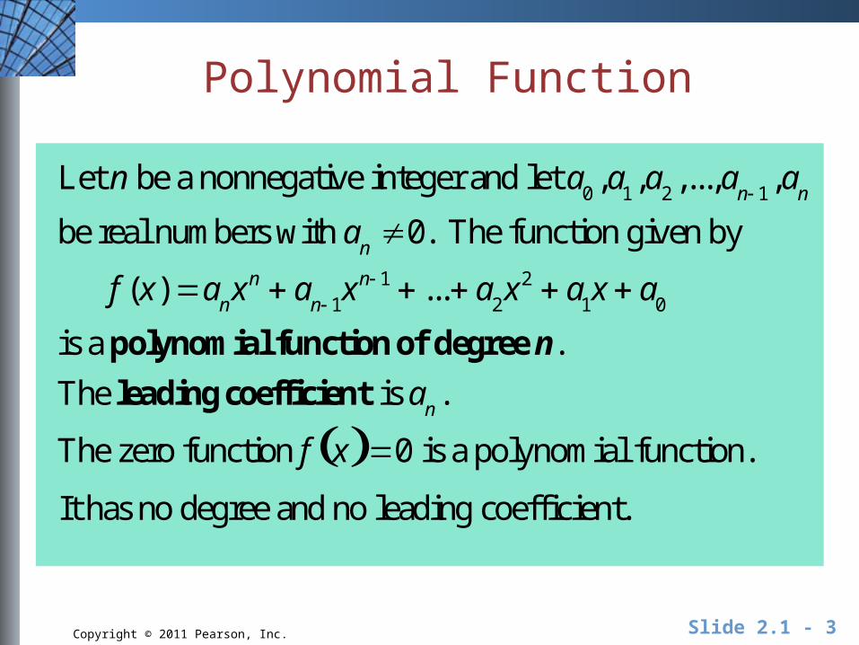
Polynomial Function
Let n be a nonnegative integer and let a0,a
1,a
2,...,a
n 1,a
n
be real numbers with an0. The function given by
f (x) anxn a
n 1xn 1 ... a
2x2 a
1x a
0
is a polynomial function of degree n.
The leading coefficient is an.
The zero function f x 0 is a polynomial function.
It has no degree and no leading coefficient.

Copyright © 2011 Pearson, Inc. Slide 2.1 - 4
Polynomial Functions ofNo and Low Degree
Name Form Degree
Zero Function f(x) = 0 Undefined
Constant Function f(x) = a (a ≠ 0) 0
Linear Function f(x) = ax + b (a ≠ 0) 1
Quadratic Function f(x) = ax2 + bx + c (a ≠ 0) 2
Copyright © 2011 Pearson, Inc. Slide 2.1 - 5
Example Finding an Equation of a Linear Function
Write an equation for the linear function f
such that f ( 1) 2 and f (2) 3.

Copyright © 2011 Pearson, Inc. Slide 2.1 - 6
Example Finding an Equation of a Linear Function
Use the point-slope formula and the point (2,3):
y y1 m(x x1)
y 3 1
3x 2
Write an equation for the linear function f
such that f ( 1) 2 and f (2) 3.
The line contains the points ( 1,2) and (2,3). Find the slope:
m 3 2
2 1
1
3
f (x) 1
3x
7
3y 3
1
3x
2
3
y 1
3x
7
3
Copyright © 2011 Pearson, Inc. Slide 2.1 - 7
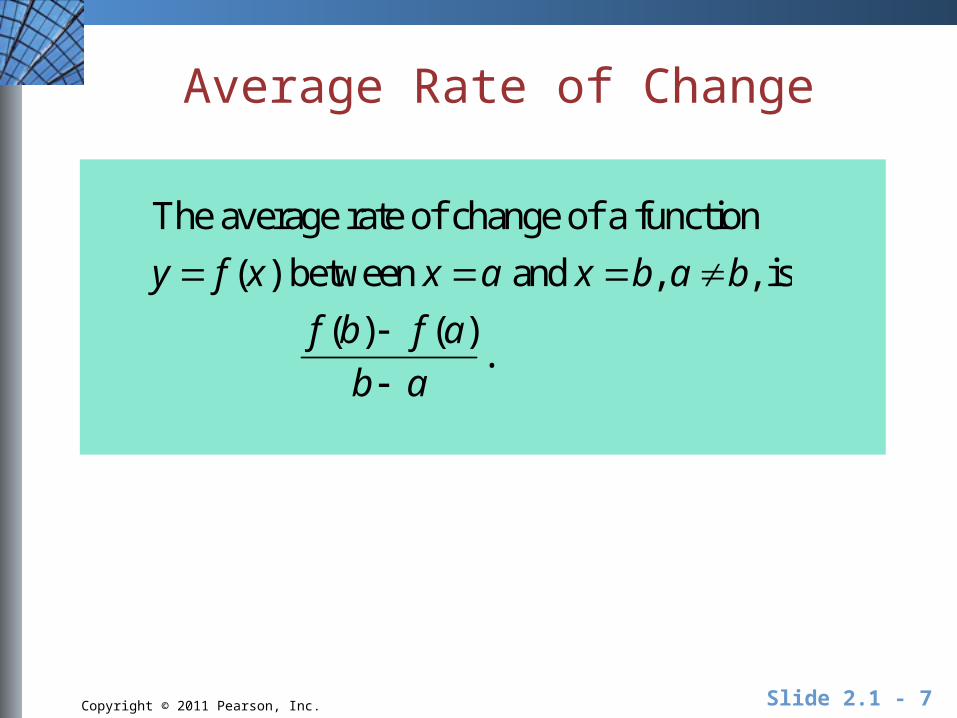
Average Rate of Change
The average rate of change of a function
y f (x) between x a and x b, a b, is
f (b) f (a)
b a.

Copyright © 2011 Pearson, Inc. Slide 2.1 - 8
Constant Rate of Change Theorem
A function defined on all real numbers is a linear
function if and only if it has a constant nonzero
average rate of change between any two points
on its graph.
Copyright © 2011 Pearson, Inc. Slide 2.1 - 9
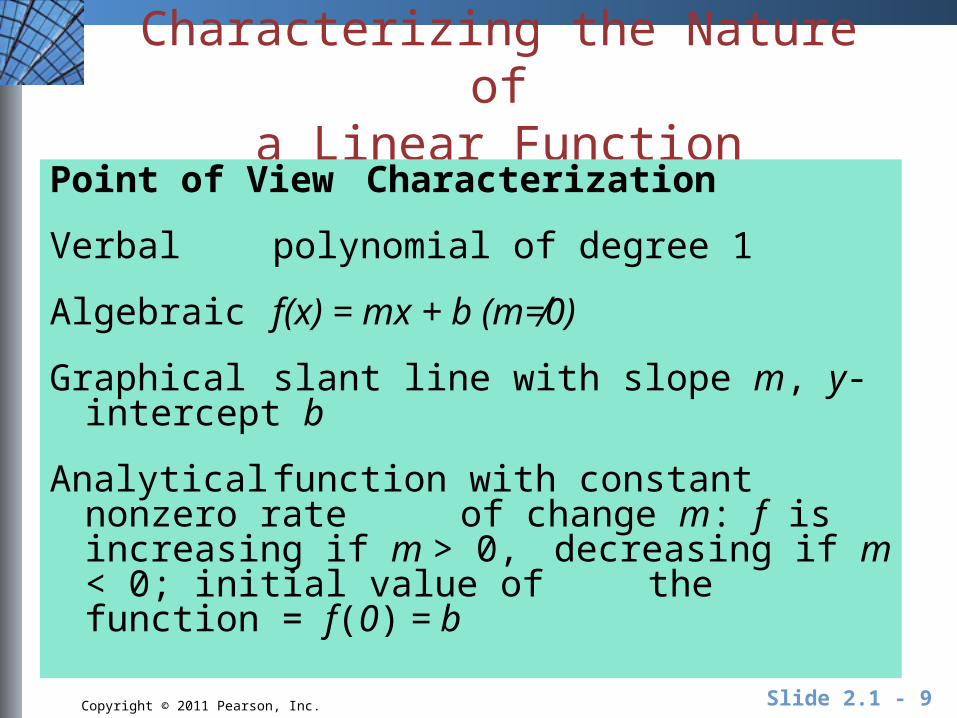
Characterizing the Nature ofa Linear Function
Point of View Characterization
Verbal polynomial of degree 1
Algebraic f(x) = mx + b (m≠0)
Graphical slant line with slope m, y-intercept b
Analytical function with constant nonzero rate of change m: f is increasing if m > 0, decreasing if m < 0; initial value of the function = f(0) = b

Copyright © 2011 Pearson, Inc. Slide 2.1 - 10
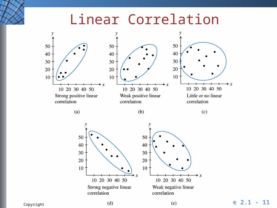
Properties of theCorrelation Coefficient, r
1. –1 ≤ r ≤ 12. When r > 0, there is a positive linear
correlation.3. When r < 0, there is a negative linear
correlation.4. When |r| ≈ 1, there is a strong linear
correlation.5. When |r| ≈ 0, there is weak or no linear
correlation.
Copyright © 2011 Pearson, Inc. Slide 2.1 - 11
Linear Correlation
Copyright © 2011 Pearson, Inc. Slide 2.1 - 12
Regression Analysis
1. Enter and plot the data (scatter plot).
2. Find the regression model that fits the problem situation.
3. Superimpose the graph of the regression model on the scatter plot, and observe the fit.
4. Use the regression model to make the predictions called for in the problem.
Copyright © 2011 Pearson, Inc. Slide 2.1 - 13
Example Transforming the Squaring Function
Describe how to transform the graph of f (x) x2 into the
graph of f (x) 2 x 2 2 3.
Copyright © 2011 Pearson, Inc. Slide 2.1 - 14
Example Transforming the Squaring Function
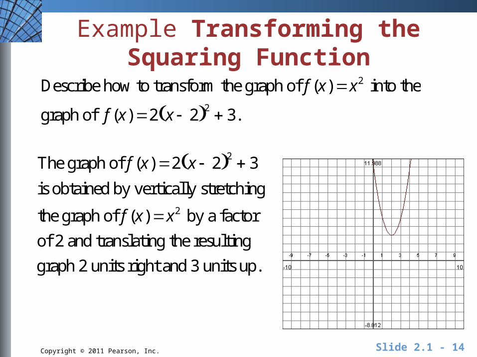
The graph of f (x) 2 x 2 2 3
is obtained by vertically stretching
the graph of f (x) x2 by a factor
of 2 and translating the resulting
graph 2 units right and 3 units up.
Describe how to transform the graph of f (x) x2 into the
graph of f (x) 2 x 2 2 3.
Copyright © 2011 Pearson, Inc. Slide 2.1 - 15
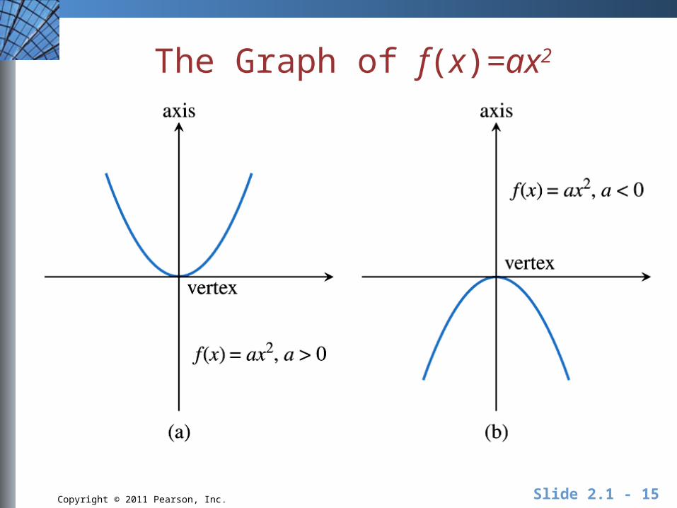
The Graph of f(x)=ax2

Copyright © 2011 Pearson, Inc. Slide 2.1 - 16
Vertex Form of a Quadratic Equation
Any quadratic function f(x) = ax2 + bx + c,a ≠ 0, can be written in the vertex form
f(x) = a(x – h)2 + k.
The graph of f is a parabola with vertex (h, k) and axis x = h, where h = –b/(2a) and
k = c – ah2. If a > 0, the parabola opens upward, and if a < 0, it opens downward.
Copyright © 2011 Pearson, Inc. Slide 2.1 - 17
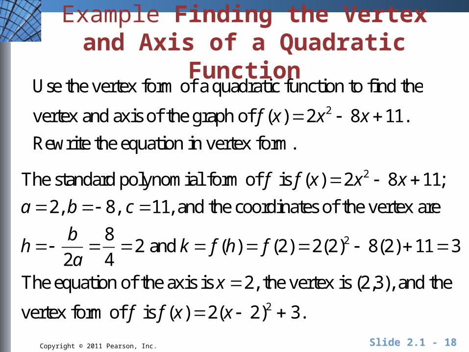
Example Finding the Vertex and Axis of a Quadratic Function
Use the vertex form of a quadratic function to find the
vertex and axis of the graph of f (x) 2x2 8x 11.
Rewrite the equation in vertex form.
Copyright © 2011 Pearson, Inc. Slide 2.1 - 18
Example Finding the Vertex and Axis of a Quadratic Function
The standard polynomial form of f is f (x) 2x2 8x 11;
a 2, b 8, c 11, and the coordinates of the vertex are
h b
2a
8
42 and k f (h) f (2) 2(2)2 8(2)11 3.
The equation of the axis is x 2, the vertex is (2,3), and the
vertex form of f is f (x) 2(x 2)2 3.
Use the vertex form of a quadratic function to find the
vertex and axis of the graph of f (x) 2x2 8x 11.
Rewrite the equation in vertex form.
Copyright © 2011 Pearson, Inc. Slide 2.1 - 19
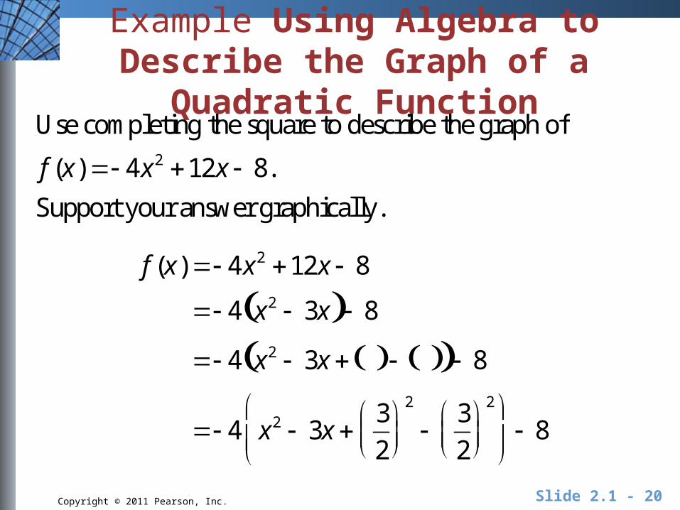
Example Using Algebra to Describe the Graph of a Quadratic Function
Use completing the square to describe the graph of
f (x) 4x2 12x 8.
Support your answer graphically.
Copyright © 2011 Pearson, Inc. Slide 2.1 - 20
Example Using Algebra to Describe the Graph of a Quadratic Function
f (x) 4x2 12x 8
4 x2 3x 8
4 x2 3x 8
4 x2 3x 3
2
2
3
2
2
8
Use completing the square to describe the graph of
f (x) 4x2 12x 8.
Support your answer graphically.

Copyright © 2011 Pearson, Inc. Slide 2.1 - 21
Example Using Algebra to Describe the Graph of a Quadratic Function
4 x2 3x 9
4
4 9
4
8
4 x 3
2
2
1
Use completing the square to describe the graph of
f (x) 4x2 12x 8.
Support your answer graphically.
Copyright © 2011 Pearson, Inc. Slide 2.1 - 22
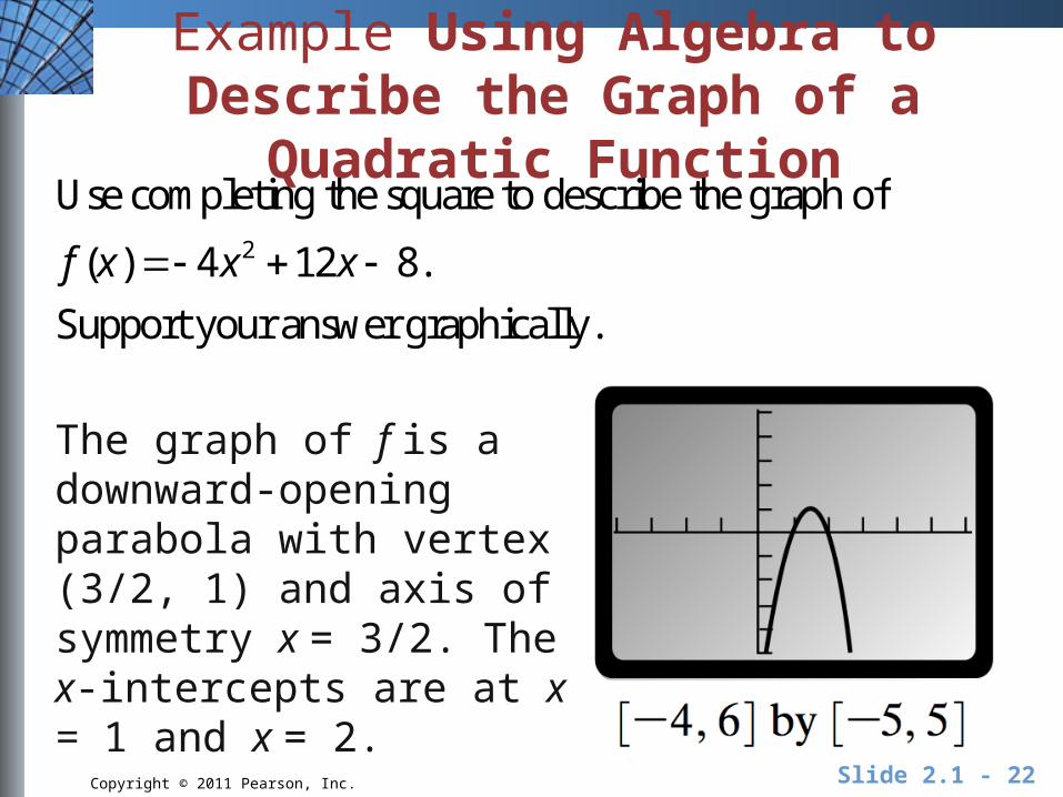
Example Using Algebra to Describe the Graph of a Quadratic Function
Use completing the square to describe the graph of
f (x) 4x2 12x 8.
Support your answer graphically.
The graph of f is a downward-opening parabola with vertex (3/2, 1) and axis of symmetry x = 3/2. The x-intercepts are at x = 1 and x = 2.
Copyright © 2011 Pearson, Inc. Slide 2.1 - 23
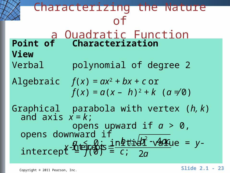
Characterizing the Nature ofa Quadratic Function
Point of CharacterizationViewVerbal polynomial of degree 2
Algebraic f(x) = ax2 + bx + c or f(x) = a(x – h)2 + k (a ≠ 0)
Graphical parabola with vertex (h, k) and axis x = k;
opens upward if a > 0, opens downward if
a < 0; initial value = y-intercept = f(0) = c; x-intercepts
b b2 4ac
2a

Copyright © 2011 Pearson, Inc. Slide 2.1 - 24
Vertical Free-Fall Motion
The height s and vertical velocity v of an object in
free fall are given by
s(t) 1
2gt 2 v0t s0 and v(t) gt v0 ,
where t is time (in seconds), g 32 ft/sec2 9.8 m/sec2
is the acceleration due to gravity, v0 is the initial
vertical velocity of the object, and s0 is its initial height.
Copyright © 2011 Pearson, Inc. Slide 2.1 - 25
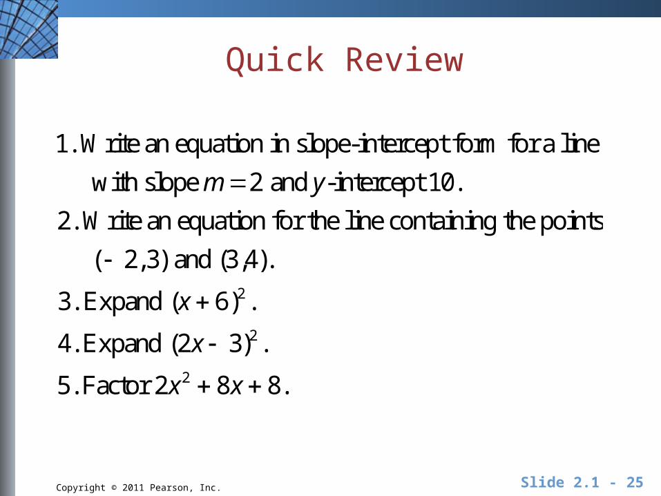
Quick Review
1. Write an equation in slope-intercept form for a line
with slope m 2 and y-intercept 10.
2. Write an equation for the line containing the points
( 2,3) and (3,4).
3. Expand (x 6)2 .
4. Expand (2x 3)2 .
5. Factor 2x2 8x 8.
Copyright © 2011 Pearson, Inc. Slide 2.1 - 26
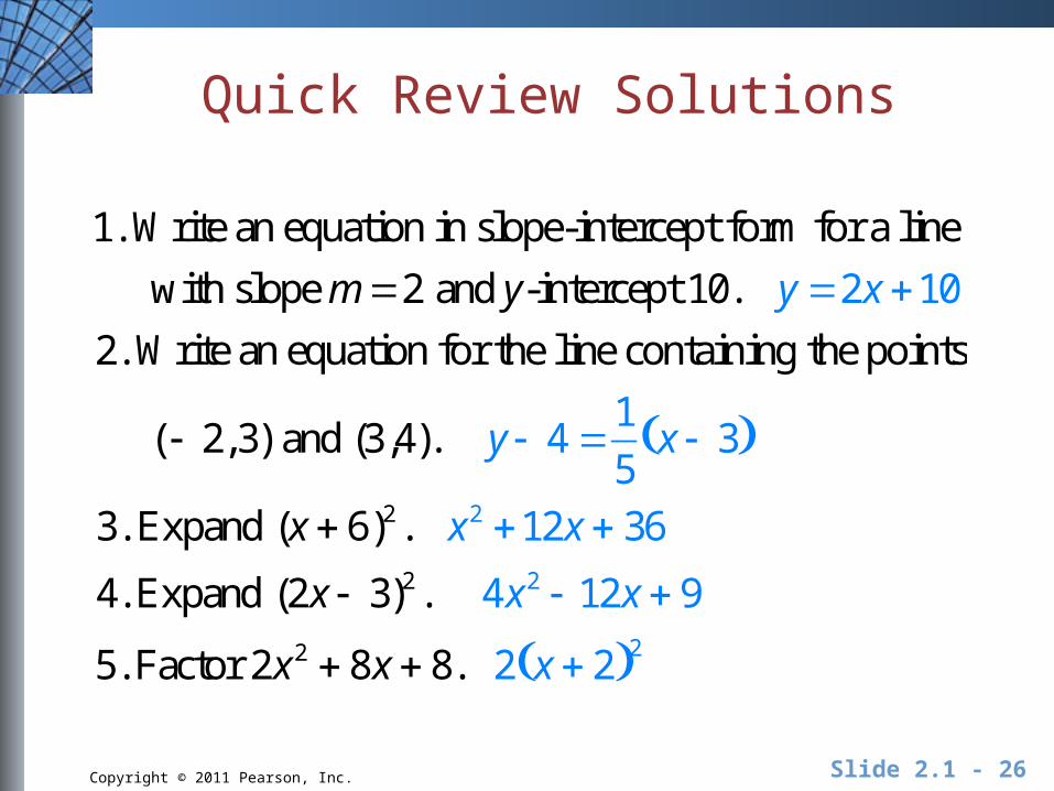
Quick Review Solutions
1. Write an equation in slope-intercept form for a line
with slope m 2 and y-intercept 10. y 2x 10
2. Write an equation for the line containing the points
( 2,3) and (3,4). y 4 1
5x 3
3. Expand (x 6)2 . x2 12x 36
4. Expand (2x 3)2 . 4x2 12x 9
5. Factor 2x2 8x 8. 2 x 2 2
Related Documents


