Copyright © 2004, Ramkamal Bhagavatula

ANALYSIS OF PDC BIT WOBBLING AND DRILLING

STRING BUCKLING

by

RAMKAMAL BHAGAVATULA, B.Tech., M.S.M.E.

A THESIS

IN

PETROLEUM ENGINEERING

Submitted to the Graduate Faculty of Texas Tech University in

Partial Fulfillment of the Requirements for

the Degree of

MASTER OF SCIENCE

IN

PETROLEUM ENGINEERING

Approved

Chairperábn of the Co Hííîítée

Accepted

Dean of the Graduate School

May, 2004

Copyright © 2004, Ramkamal Bhagavatula

ACKNOWLEDGEMENTS

I would hke to express my sincere thanks and appreciation to my academic

advisor Dr. Lloyd Heinze and graduate advisor Dr. Akanni Lawal for their excellent

guidance and constant support during my graduate studies, without which my efforts

would not have been complete and fruitful. I would also hke to express my thanks to Dr.

Paulus Adisoemarta and Dr. Akanni Lawal for their time and effort in reviewing this

manuscript and making valuable suggestions as my thesis committee members.

I am extremely grateflil to my parents and in-laws for their support and constant

encouragement throughout my academic career. I thank my wife, Saroja for being with

me against all odds and providing the moral support to pursue higher studies. I would

also like to thank Dr. J. F. Lea, all the facuhy members, and my friends who have helped

me directly or indirectly during my graduate studies.

n

TABLE OF CONTENTS

ACKNOWLEDGEMENTS ii

ABSTRACT v

LIST OF TABLES vi

LIST OF FIGURES vii

CHAPTER

I. INTRODUCTION 1

1.1 PDC Bit WobbUng 1

1.2 DrilUng String BuckUng 4

1.3 Research Objective and Scope of Study 6

II. CUTTING FORCES ON A PDC BIT 8

2.1 Orthogonal Cutting Principle 8

2.2 Emst-Merchant Minimum Energy Criterion 10

2.3 PDC Bit Force Evaluation 13

III. BIT WOBBLING MODEL 15

3.1 Strain Energies in a Stressed Body 15

3.2 CastigUano's theorem and MaxweU's reciprocal theorem 21

3.3 Forces acting upon Bit and Bottom Hole Assembly (BHA) 25

3.4 Elastic Constants of Bottom Hole Assembly 31

3.4.1 Static Conditions 31

3.4.2 Dynamic Conditions 37

3.5 Formulation of Bit Vibrations 41

3.5.1 Lateral Vibrations 41

3.5.2 Angular Vibrations 47

IV. BIT WOBBLING-CALCULATIONS, RESULTS AND DISCUSSION 50

4.1 Example Calculations 50

4.2 Results and Discussion 55

ni

V. DRILL-STRING BUCKLING: GENERALIZED ANALYTICAL 66 SOLUTION

VI. DRILL-STRING BUCKLING-ANALYSIS AND DISCUSSION 78

6.1 CriticalBuckUngConditionoftheFirst-Order 78

6. L1 Point of Tangency for First-Order Critical Condition 85

6.1.2 Equation Coefficients for First-Order Critical Condition 85

6.2 Critical Buckling Conditions above First-Order 87

6.2.1 Equation Coefficients for Critical Conditions above First- 91 Order

6.3 ShapeoftheBuckledDrillingString 92

6.4 Bending Moment Diagrams for First and Higher Buckling 96 Orders

6.5 Force Applied by Buckled Drill-String on bore-hole wall 99

VII. CONCLUSIONS AND RECOMMENDATIONS 102

REFERENCES 104

APPENDDC

A BIT WOBBLING DATA 106

B MATLAB SOURCE CODE 116

IV

ABSTRACT

Earlier study of failure of PolycrystaUine-diamond-compact (PDC) bits was

attributed to "bit-whirUng" theory which caused cutter chipping due to down-hole bit

vibrations. Based on the bit-whiri theory, the PDC bit design was modified by changing

the cutters orientation, introduction of low-friction pads around the bit so that the net

imbalance forces from the cutters are minimized. The "bit-whirl" theory by itself was not

sufficient to address the failure mechanism as it considered only the kinematics of the bit

and the geometric aspect of the bit dynamics was neglected. The study in the paper

focuses on another theory known as PDC "bit-wobbUng" which takes into account the bit

down-hole dynamics. Based on this theory, a kinetic model of the bit and the bottom-hole

assembly (BHA) is developed. The various forces acting on the model are presented and

analyzed. Sensitivity analysis is carried out on the model to study the effects of stabiUzer

position, phase angle, bit velocity, bit weight, driU-coUar stiffiiess etc. on the backward

cutter velocity. This study identifies possible solutions for reducing the bit-wobbUng.

The theory of buckUng is appUed to derive the analytical solutions to driU-string

buckUng. Based on the analytical solutions, the different buckling orders are modeled and

analyzed. The buckled driU-string and bending moment profiles of first and higher-order

buckUng are generated through computer programs given in the Appendix. The effect of

various parameters on driU-string buckUng is studied and presented.

LIST OF TABLES

4.1 Basic Input Parameters for bit wobbUng analysis 50

6.1 Values of x and xs for Critical Condition above First-Order 90

A.l Variation of AmpUtude with Frequency ratio for different viscous 107 damping factor (AmpUtude in inches)

A.2 Variation of AmpUtude Ratio with Frequency ratio for different 108 viscous damping factor (AmpUtude in inches)

A.3 Variation of Phase Angle with Frequency Ratio (Phase Angle in 109 degrees)

A.4 Cutter Velocity at Bit Center (Er = 5x\0^psi) 110

A.5 Cutter Velocity at Bit Center (Æ, = IxlO^ psi) 111

A.6 Cutter Velocity variation with Lateral Contact Area 112

A.7 Effect of Bit Weight on Cutter Backward Velocity 113

A.8 Effect of StabiUzer Position on Cutter Backward Velocity 114

A.9 Effect of DriU Collar Stiffhess on Cutter Backward Velocity for 115 given distance of StabiUzer from Bit

A.IO Effect of Damping Factor on Cutter Backward Velocity 115

VI

LIST OF FIGURES

1.1 Test-weU ROP comparison in Oswego Umestone 1

1.2 General Bit Whirl condition 3

1.3 Typical cutter paths on a whirUng bit 4

2.1 Typical configuration showing shear plane 8

2.2 Forces acting on a Chip 9

2.3 Relation between forces in metal cutting 10

2.4 Components of forces in cutting face of tool 10

2.5 Relation between forces and angles in orthogonal metal cutting 11

3.1 Normal and shear stresses at a point in a body 15

3.2 Normal forces and strain energy stored in a body 17

3.3 Shear forces and shear strain energy stored in a body 18

3.4 Energy in beams subjected to a uniform bending moment 20

3.5 Influence coefficients for beam deflections 22

3.6 Work done on a beam in sequence (a) and (b) 23

3.7 GeneraUzed forces and corresponding displacements in an elastic body 24

3.8 Free-Body Diagram of a BHA in vertical hole 27

3.9 Free-Body diagram of a bit in a vertical hole 27

3.10 Dynamic equiUbrium of a BHA in a vertical hole 37

3.11 Cantilever beam with an end load 38

4.1 Path of bit center at resonance condition 56

4.2 Path of bit center at non-resonance condition (Frequency ratio=0.88) 56

4.3 Path of bit center at non-resonance condition (Frequency ratio=1.30) 57

4.4 Variation of AmpUtude with Frequency Ratio 57

4.5 Variation of AmpUtude Ratio with Frequency Ratio 58

4.6 Variation of Phase Angle with Frequency Ratio 58

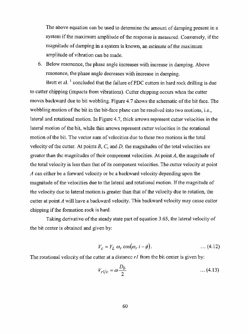
4.7 Cutter Velocifies on a PDC bit face 61

4.8 Velocity of cutter at bit center {Er = 5x10^psi) 62

vu

4.9 Velocity of cutter at bit center {Er = IxlO^psi) 62

4.10 Effect of Lateral Contact Area on Cutter Backward Velocity 63

4.11 Effect of Weight of Bit on Cutter Backward Velocity 64

4.12 Effect of StabiUzer position on Cutter Backward Velocity 64

4.13 Effect of StabiUzer position on Cutter Backward Velocity 65

4.14 Effect of Viscous Damping Factor on Cutter Backward Velocity 65

5.1 Extemal forces acting upon a DrilUng String 66

5.2 Extemal Forces acting on a driUing string section 68

5.3 Vectorial representation of forces on a drilling string section 69

5.4 Functions of F(x), P(x), and S{x) 76

5.5 Functions ofG{x), Q{x), and T(x) 76

5.6 Functions of//(x), R(x), and U(x) 77

6.1 Critical Condition of the First-Order 79

6.2 Length of a dimensionless unit with change in drilling mud density 80

6.3 Critical Weights on bit for First-Order Critical BuckUng 81

6.4 Buckling Conditions for Combination DriUing Strings 83

6.5 Influence of Drill-CoUar size on BuckUng (I.D=1.875-m) 83

6.6 Influence of Drill-CoUar size on BuckUng (I.D=2.5-/>z) 84

6.7 Influence of DriU-CoUar size on Buckling (LD=3.0-z>2) 84

6.8 Shape of Buckled Curves for Different BuckUng Orders 93

6.9 Tangency and Neutral Points Variation with different BuckUng Orders 94

6.10 Critical Weights on Bit for Second-Order Buckling 96

6.11 Bending Moment Coefficient Profile for First-Order BuckUng 97

6.12 Bending Moment Coefficient Profile for Second-Order BuckUng 98

6.13 Bending Moment Coefficient Profile: Second buckle contacts bore-hole 98 waU

6.14 Coefficient/for calculating force on bore-hole waU due to driU string 100 buckUng

6.15 Force of Buckled DriUing String (Second Buckle Contacts Bore Hole 100 WaU)

vni

CHAPTER 1

INTRODUCTION

l . lPDCBitWobbUng

PDC bits were introduced in the early 1970s and have then almost replaced three-

cone bits for use in relatively soft, non-abrasive formations. The main Umitation of PDC

bits is when driUing in harder formations or even in softer formations with infrequent

hard streaks. The usuaUy high polycrystaUine-diamond compact (PDC) bit wear Umits its

Ufe for use in hard formations even though higher penetration rates can be achieved with

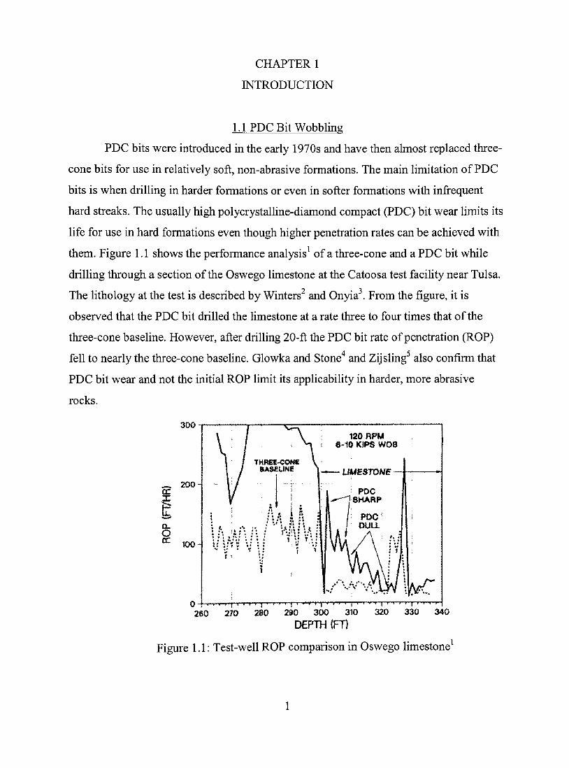
them. Figure 1.1 shows the performance analysis^ of a three-cone and a PDC bit while

drilling through a section of the Oswego limestone at the Catoosa test faciUty near Tulsa.

The lithology at the test is described by Winters and Onyia . From the figure, it is

observed that the PDC bit driUed the Umestone at a rate three to four times that of the

three-cone baseline. However, after driUing 20-ft the PDC bit rate of penetration (ROP)

fell to nearly the three-cone baseUne. Glowka and Stone"^ and Zijsling^ also confirm that

PDC bit wear and not the initial ROP limit its appUcabiUty in harder, more abrasive

rocks.

300

cr: X

o ir

200-

100-

120 HPU 6-10 KIPS WOØ

TKRte-CONC ÍIAS£UNE

: *J\ íî íî

í

260 270 280 290 300 310 320 330 340

DEPTH (FT)

Figure 1.1: Test-well ROP comparison in Oswego Umestone^

From analysis of the drag-bit wear model by Warren,^ it is shown that the

performance of a sUghtly duU PDC bit can actuaUy be much worse than that of a three-

cone bit. This is because the bearing area increases as the wear-flats grows and this

reduces the stresses induced in the rocks. It has been observed by Zijsling^ that an

apparently duU PDC bit, i.e., one with significant wear flats can stiU driU almost as fast as

a new bit because of diamond table lips provided above the tungsten carbide. This

diamond Ups acts as the contact area and not the complete tungsten-carbide wear-flat due

to which the high contact rock stresses are stiU maintained. The presence of diamond Ups

is important for efficient driUing in hard formations. However, they are not critical while

driUing softer formations. A sharp bit is one which has diamond Ups provided on enough

cutters to cut the bottom of the hole completely. A duU bit is one that does not have

enough Ups on the cutters to cover the entire hole. PDC bits with diamond Ups are able to

outdriU PDC bits by two mechanisms: (1) they create higher contact stresses because

only the diamond contacts the formation on a sharp PDC bit, and (2) they are able to

clean the bottom of the hole mechanically and are therefore not as greatly affected by

mud, hydrauUcs and rotary speed.

PDC bits fail mainly due to cutter chipping. Warren and Sinor '' have shown that

steady-state loads applied to PDC cutters under most normal driUing situations are too

low to cause cutters to chip. Even fatigue from cycUc loading of the bit is not attributed to

the cutter chipping. It was observed from laboratory driUing^ that failure occurs mainly

due to impact loading caused by bit vibrations which were so severe that it caused PDC

studs to break and numerous cutters chipped. Even though force balancing on the PDC

bits was carried out, the primary cutter chipping mechanism due to bit vibrations could

not be overcome initiaUy. Warren et al^ has shown that cutters that chip develop wear

flats very quickly. Once a diamond table is lost because of chipping, the tungsten-carbide

wear process proceeds very quickly. They also observed that a "low-friction" bit design

can substantiaUy eliminate bit whiri. The low firiction design is based on placing the

cutters so that the net imbalance force from the cutters is directed towards a smooth pad

that slides along the well bore waU. The detrimental effects caused by impacts loads are

attributed to a phenomenon caUed "bit whiri" or bit "backward whiri." Bad bearing

design was known to produce the bit whiri. With bit whiri as shown in Figure 1.2, the bit

moves primarily laterally around the hole. The bit acts as a pinion in a hole that acts as a

gear. The drilUng imbalance pushes one side of the bit against the borehole wall creating

a new fiictional force. A clockwise torque on the bit combined with this frictional force

moves the instantaneous center of rotation away from the geometric center and towards

the wellbore waU.

Hole

Hole Center

Bit Centør

Figure 1.2: General Bit Whirl condition'

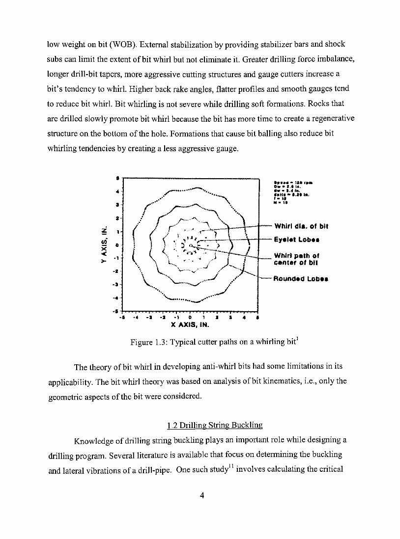
Figure 1.3 shows the typical cutter paths on a whirUng bit. It is observed that the

cutters can move backward, sideways, and farther per revolution than those on a tme

rotating bit. As a result, they are subjected to high impact loads. On a whirUng bit, a

cutter impacts the side of the well bore many times per revolution. The detrimental effect

of bit whirl is that it cannot be stopped once started. Hence, bit whirl occurs when the

dynamic forces on a bit cause the center of rotation to move as the bit rotates. A whirling

bit cuts an overgauge hole, and the cutters move faster, backwards, and sideways and

consequently are subjected to high impact loads. Once a bit begins to whirl, forces are

generated that reinforce this tendency. Bit whirl is worse at higher rotary speeds because

the centrifiigal forces are squared as rotary speeds double. Bit whirUng becomes severe at

low weight on bit (WOB). Extemal stabilization by providing stabiUzer bars and shock

subs can limit the extent of bit whirl but not eUminate it. Greater driUing force imbalance,

longer driU-bit tapers, more aggressive cutting structures and gauge cutters increase a

bit's tendency to whirl. Higher back rake angles, flatter profiles and smooth gauges tend

to reduce bit whirl. Bit whirUng is not severe while driUing soft formations. Rocks that

are driUed slowly promote bit whirl because the bit has more time to create a regenerative

stmcture on the bottom of the hole. Formations that cause bit baUing also reduce bit

whirling tendencies by creating a less aggressive gauge.

4

2

<

•4

i

' •-N

/ y —\ \

\ 'i • . . • ..' i T

V^ V

. ^ • • * • : • • * •

DM • f . « Ift.

Whlrl di«. of bU

Ey«t«t Lobttt

WMrl palh of conter ol bll

Roundod Lob««

*A -4 -a *a * i 0 1 i s 4 i X AXISt iN.

Figure 1.3: Typical cutter paths on a whirling bit

The theory of bit whirl in developing anti-whirl bits had some limitations in its

appUcability. The bit whirl theory was based on analysis of bit kinematics, i.e., only the

geometric aspects of the bit were considered.

1.2 DriUing String Buckling

Knowledge of driUing string buckUng plays an important role while designing a

driUing program. Several Uterature is available that focus on determining the buckUng

and lateral vibrations of a driU-pipe. One such study^^ involves calculating the critical

buckUng loads and natural frequencies of lateral vibration modes for a long vertical pipe,

suspended in a fluid, simply supported at the top and vertically guided at the bottom.

Another study aims at determining the critical weights and natural frequencies for

different end conditions. The fatigue and failure analysis of a drill-string^^ plays an

important role when driUing into deeper formations. Without weight on the bit, a drilUng

string wiU be straight if the hole driUed is straight. With a sufficienfly smaU weight on

bit, the string remains straight. As the weight on the bit is increased, a so-caUed critical

value of the weight is reached for which the straight form of the string is no longer stable.

The driUing string buckles and contacts the waU of the hole at a point caUed the point of

tangency. If the weight on the bit is fiirther increased, a new critical value is reached at

which the driU-string buckles a second time. This is termed as the buckUng of the second

order. With stiU higher weights on the bit, buckling of the third and higher orders occur.

At the point of tangency, the driUing string rabs against the wall of the hole, and

this cause caving in the formation. The rabbing effect becomes worse when the force

between the buckled pipe and the wall of the hole increases. When the buckled string is

rotated, some reversing stresses due to bending are created. These stresses increase with

the diameter of the hole and result in the fatigue failure of the hole. As soon as a driUing

string buckles in a straight hole, the bit is no longer vertical and a perfectly vertical hole

cannot be driUed. A certain point of a driUing string is usuaUy designated as the "neutral

point." The "neutral point" is defmed as a point in the drilUng string below which the

weight of the driUing string in mud is equal to the weight on the bit. Each value of the

weight on bit corresponds to a value of the distance between the bit and the neutral point.

The critical value of this distance depends upon the type of pipe or driU coUars and the

density of the driUing mud. The distance between the bit and the neutral point is

measured in terms of dimensionless units so that the resuUs obtained are indep§ndent of

the type of pipe, coUars, and mud.

1.3 Research Objective and Scope of Studv

The kinematic relationships derived for the bit whirl theory were used to describe

the lobed pattems observed in the field and laboratory. Analysis of bit kinetics

(kinematics and dynamics) which also account for the dynamic forces acting on the bit

would give further insight into the various parameters that affect the bit whirUng. This

study presents a "Bit WobbUng" model that is based on the bit kinetic analysis. The

eventual goal of this research is to develop a mathematical model that can characterize

the influence of various parameters on bit wobbling and broaden its appUcabiUty to a

better understanding of bit wobbUng. The results obtained from this model would help in

understanding the parameters affecting bit wobbUng and eventuaUy lead to incorporating

these factors in the design of PDC bits that can further reduce wobbUng.

The influence of the foUowing forces on the bit is considered in the modeU

a. Forces from the BHA (Bottom Hole Assembly),

b. Forces from the adjacent bore-hole waU,

c. Cutting Forces on the bit,

d. Forces from driUing fluid and stabiUzer.

The study of driUing string buckUng includes formulation of a generaUzed

dimensionless solution that can be used for any driU-pipe and driU collar size. The critical

values of weight on the bit and the shape of a buckled drilling for first and second

buckling orders are determined. The magnitude of the forces acting at the first buckle for

these buckling orders is also determined. Finally, the bending moment diagrams are

generated that help in evaluating the bending moments acting along the length of the

drilling string. The results from this study give an in-depth understanding of the buckling

principles involved and yield solutions to the various factors affecting buckling and how

to minimize or avoid buckling.

The bit kinetic analysis presented in this study is limited to the analysis of PDC

bits only. It cannot be used for analysis of three cone bits, rock bits and other commercial

types of bits. This is because the cutting forces evaluation for PDC bits are derived from

the theory of metal cutting principle. The similar principle cannot be appUed for other

types of bits as the cutting action is different for different types of bits. The cutting forces

are also dependent on the geometry of the bit and the alignment pattem of the cutting

faces on the bit. The effect of weight on the bit and rotary speed on the bit vibrations is

not taken into account in this model as the effect of drilling parameters on the

fluctuations in cutting torque and cutting forces are not clearly known. It is anticipated

that using higher weight on bit and shock absorbers will be helpfial in reducing

fluctuations in the cutting torque and cutting force, and therefore backward velocity.

Although increasing rotary speed may reduce the backwards velocities of gauge cutters, it

wiU not significantly affect the backward velocities of cutters near the bit center because

of less rotational velocity contribution to the total velocity near the bit center.

The drilling string buckling analysis study is limited to drill-strings having

constant material properties for both the drill-pipe and the drill collar throughout the

entire considered length. As the analysis is performed using numerical methods, the

results obtained represent the approximate values. For analysis simplification, the length

of a one-dimensional unit is considered to be approximately equal for both the drill collar

and the drill-pipe. The length of a one-dimensional unit of the drill collar is taken as the

dimensionless unit for the entire drilling string in the analysis. The material properties

and stiffiiess of the drill-pipe and drilI-coUar couplings on the drilling string buckling

tendency is assumed to be negligible in the analysis.

7

CHAPTER 2

CUTTING FORCES ON A PDC BIT

2.1 Orthogonal Cutting Principle

The cutting forces on PDC bit cutters are determined based on the theory of metal

cutting principles. Figure 2.1 shows a typical confíguration where the tool is considered

stationary and the work-piece is moved to the right. There is a plane in the work-piece

just ahead of the cutting tool where the shearing stress is a maximum. If the metal is

ductile so that it does not fracture initially, then there will be a plastic flow along this

plane called the shear plane.

^c-^

•* c t

-ô^ /Ch,p f \ "^^ /

_ 'ii^^^r;:. Workpie

:-J Tool \

ce'':ry^' '/''V:'-\--''ÍfC.

Figure 2.1: Typical configuration showing shear plane Source: Paul H. Black*^ - Theory ofMetal Cutting, 1961.

Thus, the chip is formed by plastic deformation of the grain stracture of the metal

along the shear plane. The angle that the shear plane makes with the horizontal is called

the shear angle, ø. The chip generated due to the shearing of the work-piece material

glides upward along the cutting face of the tool. The angle the cutting face of the tool

makes with the normal to the fmished surface is called the rake angle, a. A relief angle is

provided between the bottom face of the tool and the machined surface. This is necessary

to prevent rabbing between the tool and the machined surface due to fiiction.

The orthogonal or two-dimensional type of cutting is used to determine the

cutting forces as it is a relatively simple model rather than the more complicated oblique

cutting or three dimensional cutting. The oblique cutting model is developed from the

principles of the orthogonal cutting model. Orthogonal cutfing is "the case where the

8

cutting tool generates a plane surface parallel to an original plane perpendicular to the

direction of relative motion of the tool and work-piece. The forces acting on the chip in

orthogonal cutting are shown in Figure 2.2 (a) and are as follows: Force Fs is the

resistance to shear of the metal in forming the chip. This force acts along the shear plane.

Force F„ is normal to the shear plane and is a "backing-up" force on the chip provided by

the work-piece. Force A''acting on the chip is normal to the cutting face of the tool and is

provided by the tool. Force F is the fiictional resistance of the tool acting on the chip.

This force acts downwards against the motion of the chip as it glides upward along the

tool face. Figure 2.2 (b) shows the forces acting on the chip in which the resuUant of the

forces Fs and F^ and the resultant of the forces F and A are represented by R and R

respectively. There are only two combined forces, i.e., i? and R that are acting on the

chip. There are extemal couples that act on the chip and curl it but they are neglected in

this analysis. For equilibrium to exist, the two forces R and R must be equal in magnitude

and opposite in direction and have the same line of action. The components of the force

of the work-piece on the chip are the shear force Fs and the normal compressive force F„.

Figure 2.2: Forces acting on a Chip Source: Paul H. Black^^ Theory ofMetal Cutting, 1961

Figure 2.3 shows a composite diagram in which the two force triangles of Figure

2.2(b) have been superimposed by placing the two equal forces R and R together. Since

the angle between Fs and Fn is a right angle, the intersection of these forces Ues on a

circle of diameteriî. The horizontal force component Fc and the vertical force component

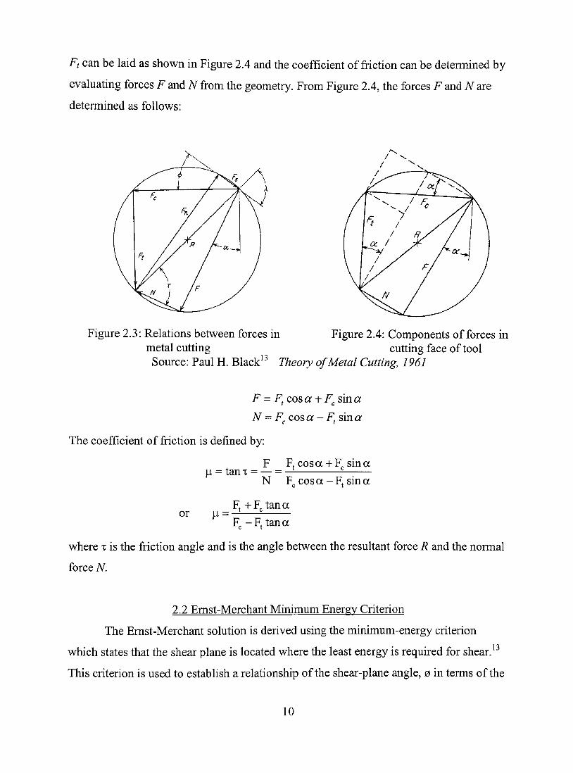
Ft can be laid as shown in Figure 2.4 and the coefficient of fiiction can be determined by

evaluating forces F and N from the geometry. From Figure 2.4, the forces F and A are

determined as follows:

Figure 2.3: Relations between forces in Figure 2.4: Components of forces in metal cutting cutting face of tool

Source: Paul H. Black^^ Theory ofMetal Cutting, 1961

F = F. cos a + F sin a

N = F^ cosa - F, sina

The coefficient of fiiction is defined by:

F K cosa + F„ sina |a = tanT = — = —

N F„ cosa-F j sina

or 1 = Fj +F^ tana

F -F^ tana

where T is the friction angle and is the angle between the resuUant force R and the normal

force N.

2.2 Emst-Merchant Minimum Energy Criterion

The Emst-Merchant solution is derived using the minimum-energy criterion

which states that the shear plane is located where the least energy is required for shear. ^

This criterion is used to establish a relationship of the shear-plane angle, ø in terms of the

10

rake angle, a and the friction angle, T. The derivation of the Emst-Merchant equation is

based on the following assumptions:

1. There is orthogonal cutting.

2. The shear strength of the metal along the shear plane is not affected by the

compressive (normal) stress acting on that plane.

3. The energy required for separafion of chip elements is negligible and the

minimum energy criterion establishes the plane on which the shearing formation

occurs.

In beginning a cut in metal cutting operation, as the cutting force Fc increases

gradually, the shear stress on various planes ahead of the tool will increase along with Fc

but the stress wiU not be the same on all planes ahead of the tool because the shearing

components of the forces on the planes are not the same. On one of the planes, however,

the shear stress wiU be greater than on any other, and as F^ is fixrther increased, the shear

stress on that plane will reach the yield strength in shear of the material being cut and

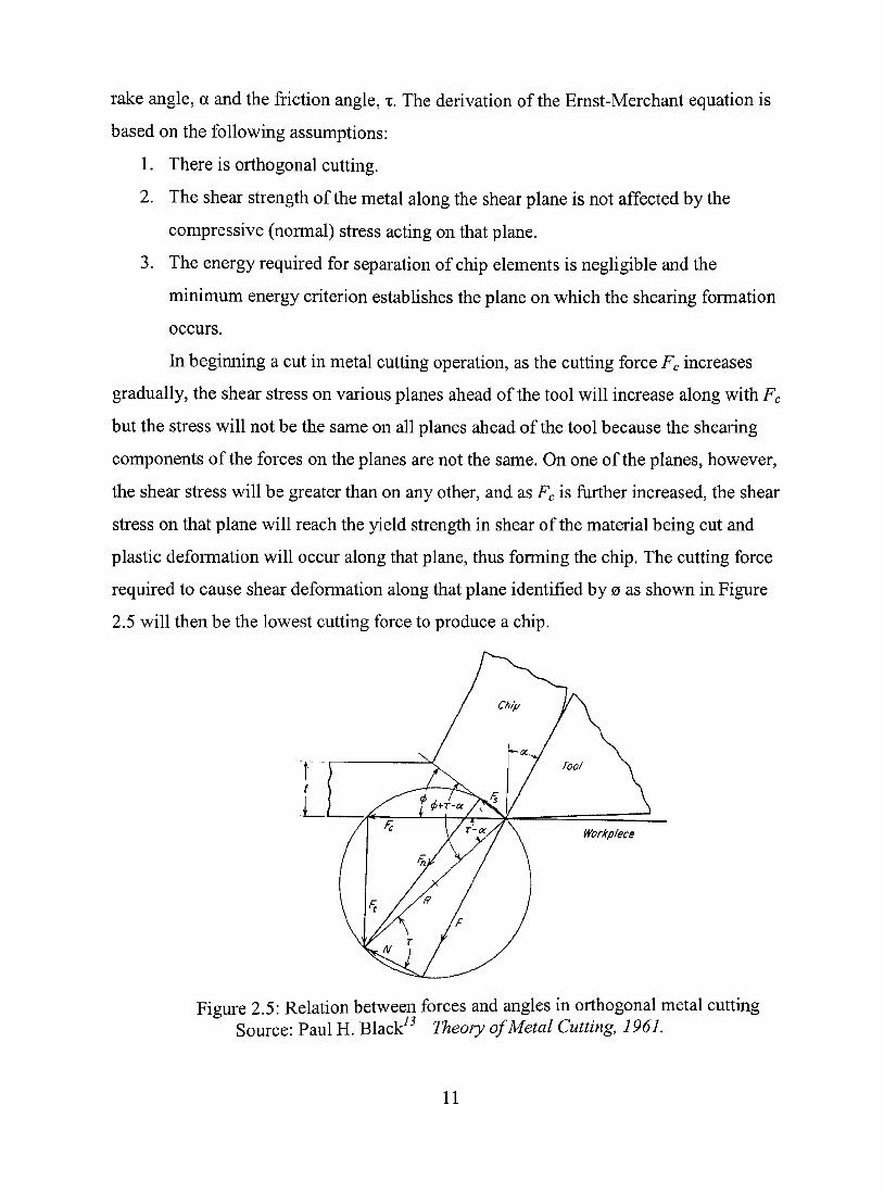
plastic deformation will occur along that plane, thus forming the chip. The cutting force

required to cause shear deformation along that plane identifíed by ø as shown in Figure

2.5 will then be the lowest cutting force to produce a chip.

Figure 2.5: Relation between forces and angles in orthogonal metal cutting Source: Paul H. Black^^ Theory ofMetal Cutting, 1961.

11

Shear deformation along any other plane would require a greater cutting force, but

after shear deformation begins on one plane, the cutting force cannot exceed that

minimum value. This process is an applicafion of the principle of minimum energy in that

the cutting force F^ is responsible for the work done in metal cutting, so that, for given

rake angles a and friction angles T, the shear-plane angle ø wiU assume such a value as to

make the energy required or work done by Fc a minimum. To determine the shear plane

angle (p, an equation for the cutting force Fc is developed in terms of ø and differentiated

with respect to cp. The resulting equation is equated to zero and solved for the angle ø.

From the geometry of Figure 2.5, we get

F. = iî cos(r - a)

F^ = R cos((Z> + r - a)

or p^^F,cos(T-a) ^ ^ ^ cos((z} + r - a )

If the cross-sectional area of the un-deformed chip be represented by A, then the

area of the shear plane will be equal to A/sin ø. The force Fs on the shear plane can be

replaced by the stress on the plane multiplied by the area, or

sin^

Substituting the above equation in equation 1, we get

SÂcos(r-a) ^^ ^^ Fc = ^ — • ...(2.2)

sin^cos(^ + r-í:ir)

Differentiating equation (2.2) with respect to the shear angle, ø and equating to zero,

we get

dF , ^ - cos é cos(tí) -\-T -a) + siné sin(fí) + r - a) — - = S,A cos(r -a)x = 0

d^ sin (zícos ((p-\-T-a)

cos cos((z) + r - ûr) - sin (Zí sin((z) + r - a) = 0

cos((Z) + (z) + r - a ) = 0 cos(2^ + r - a ) = 0

12

2^ + r - ûr = — or 2

, ;r a r < = T + T - : 7 • ...(2.3)

4 2 2

2.3 PDC Bit Force Eva uafíon

The forces on the PDC bit are evaluated by applying the Emst-Merchant

minimum energy criterion. From equation (2.2), we get

SAcos(T-a) F„ =

sin^cos(^-\-T-a)

SÂcos(T-a)

sin (z)[cos (^ COS(T -a)- sin sin(r - a)]

_ iS^^cos(r-a)

— [2sin^cos(^cos(r -a)-2sin^ ^sin(r - a ) \

_ 2SÂcos(T-a)

[sin 2(z) cos(r -a)-(l- cos 2(Z>) sin(r - a)]

2SÂcos(T-a)

[sin 2^ cos(r - ÛT) + cos 2^ sin(r -a)- sin(r - ÛT) J

_ 25'^^cos(r-a)

[sin(2^ + r - ûí) - sin(r - a)]

71

But, 2<f)-\-T-a = — from equation (2.3), hence above equationbecomes

25',^cos(r-<:ir)

sin(—)-sin(r-a) 2

îS^^cos^r-ûr)

1 - sin(r - a)

^^_2S,Acos{T-a) ^2.4) 1 - sin(r - a)

The above equation represents the force on the bit in the vertical direction.

13

Similarly, the force Ft from Figure 2.5 is given by:

P SÂsin(T-a) ^2.5) sin^cos((ZÍ + r - a )

Applying the above procedure to evaluate the denominator of equation (2,5) along with

the minimum energy criterion, we get the fínal form of equation (2.5) as

P ^2SÂsin(T-a) ...(2.6) 1 - sin(r - a)

The above equation represents the force on the bit in the horizontal direction.

14

CHAPTER 3

BIT WOBBLING MODEL

3.1 Strain Energies in a Stressed Bodv

Before the mathematical model of Bit Wobble is derived, the different kinds of

strain energy that can be stored in a stressed body are considered initially. The concept of

strain energies are applied in generating the model that will be discussed later. The

different types of strain energies are:

a. Strain energy due to direct shear,

b. Strain energy due to normal stress,

c. Strain energy due to torsional load,

d. Strain energy due to bending.

y\

Figure 3.1: Normal and shear stresses at a point in a body Source: A.H.Burr, J.B.Cheatham^^, Mechanical Analysis andDesign,

(2"Êdition), 1999.

Consider a body subject normal stress o and shear stress T as shown in Figure

3.1.^^ Normal strain or unit elongation is designated by s and shearing strain or angle of

distortion by y. The modulus of elasticity, shear modulus and Poisson's ratio are

represented by E, G, and y, respectively. In an orthogonal coordinate system, the

elasticity stress-strain relations are given by

15

and

^x = (^x-r(<^y+crz)]

^y=-[(^y-r{<^x+(^z)]

^z=-[rz-r(cr;,+c7y)]

• (3 .1)

=1 - 1 -1 rxy ^ ^xy ' ryz - „ '^yz ' ^zx ~ ^ ^zjc

(3.2)

In Figure 3.1, the first subscript to a shear stress T indicates the direcfion of the

normal to the plane on which it acts, and the second subscript indicates the direction of

the stress on this plane. Asr^y = yx xy '^zy yz andr^^ = \T^J , the three equations of

equation 3.2 are suffícient. Moduli G and E are related by

G = 2(l + r)'

. . .(3.3)

The unit change in volume of an element with sides of initial length dx, dy and dz

is called the volume expansion e, and it is seen to be the sum of the volume changes in

each direction divided by the initial volume, i.e.,

e = (s^dx)dy dz + (Sydy)dz dx + (s^dz)dx dy

dx dy dz — S-^ -\- S y + S^^ . (3.4)

Substitution of equations 3.1 into equation 3.4 gives the following linear

relationship between volume expansion and the sum of any orthogonal set of normal

stresses. If w, v, and w denote the displacements of a particle in the body along the^, Y,

16

and Z axes, respectively, then the stresses and strains can be represented by the following

equations:

^x^ du

dx ^y =

ÔV

dy ^z =

dw . (3.5)

du dv yxy=—'^

ôv dw

ôy dx' ^y^'dz'^ dy' ^''~ - ^

dw du — + — dx dz

(3.6)

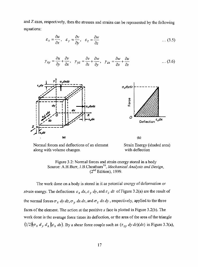
I y\ aydxdz

Normal forces and deflections of an element along with volume changes.

Oxdydz

Defiection z^x

(b)

Strain Energy (shaded area) with deflection

Figure 3.2: Normal forces and strain energy stored in a body Source: A.H.Burr, J.B.Cheatham , Mechanical Analysis and Design,

(^"'Êdition), 1999.

The work done on a body is stored in it as potential energy of deformation or

strain energy. The deflections s^ dx, Sy dy, and s^ dz of Figure 3.2(a) are the result of

the normal forces CTJ^ dy dz, a^ dx dz, and a^ dx dy , respectively, applied to the three

faces of the element. The action at the positive x face is plotted in Figure 3.2(b). The

work done is the average force times its deflection, or the area of the area of the triangle

{\I2}^^ dy d^ j^Sy. dx). By a shear force couple such as (T^y dy dz)(dx) in Figure 3.3(a),

17

the work done is its average value times the angular deflection y^y l^ that it causes. By

the two couples on the element, the total strain energy due to direct shear on two opposite

faces is given by:

[/,. =(l/2)(r,^ dy dz){dx){Y^j2)^(\l2)(T^^ dx dz){dy)(r,j2) = (l/2)T^^ r.y dx dy dz.

The total strain is given by

U,t = (1 / 2)(T^y rxy + T^yz Yyz + zx Yzx )dx dy dz (3.7)

or, Strain Energy per unit volume is given by

Ustv = (1 / ^)(^xy Yxy + V ^y^ ^ ^^^ ^^^ ^

Xyj^xdz {x^/iydz)dx

Jydz

(a)

Angular changes due to Shear forces and distortion of an element

J2> a D O

o to

x:

Angíø

(b)

Strain energy with angular distortion due to shear-force couple

Figure 3.3: Shear forces and shear strain energy stored in abody Source: A.H.Burr, J.B.Cheatham^^ Mechanical Analysis andDesign.

(2"Êdition), 1999.

18

If the body is acted upon only by shear forces, then in general the strain energy

due to direct shear can be defined by

Strain Energy = (1/2)* Z (Shear Stress * Shear Strain) * Volume of body.

Similarly by considering the area of triangle in Figure 3.2(b), the strain energy due to

normal stress is given by:

Uat ={^l2)((7^s^+c7ySy^(j^ s^)dxdydz. ... (3.8)

If the body is acted upon only by normal forces, then in general the strain energy due to

direct normal stress can be defined by

Strain Energy = (1/2)* 2 (Normal Stress * Normal Strain) * Volume of body.

From equation 3.7, the strain energy can be represented by [7^ = V where V 2 G

is the volume of the body. If the cross-secfíon of the body is circular as in case of a drill-

pipe, then the cross-secfíonal area at any point at distance x from the axis of the shaft is

given by:

da = 2 xdx and

Volume, dV= l "^ 2"^ "^ dx.

For a hollow drill-pipe, the torsional stress varies from zero at the central axis to a

maximum stress at the outside diameter. Let the magnitude of the maximum shear stress

be T at the outer surface. Then the shear stress at a given section is defined by:

X

q = rx — Ri

where R^ = extemal radius of the drill pipe.

2 Strain energy stored at this section = —— XIXITVxdx

19

^2 2 X— - -x lx ln xdx

2C R}

xlnl X dx. 2CRI

The total strain energy is stored in the drill-pipe is obtained by integrating the above

equation from intemal radius, Ri to extemal radius R^.

R 2 _2

— xlnlx dx 2CR2 R,

T nl

CRI

X R.

-^R.

'-i(4-Rí) ACRI

^"^^"^^KiRl-Rhl='"^^''^'^ AC R2 4C DI

V ...(3.9)

Figure 3.4: Energy in beams subjected to a uniform bending moment Source: A.H.Burr, ].B.Cheatham^\MechanicalAnalysis and Design.,

(2"* Edition), 1999.

20

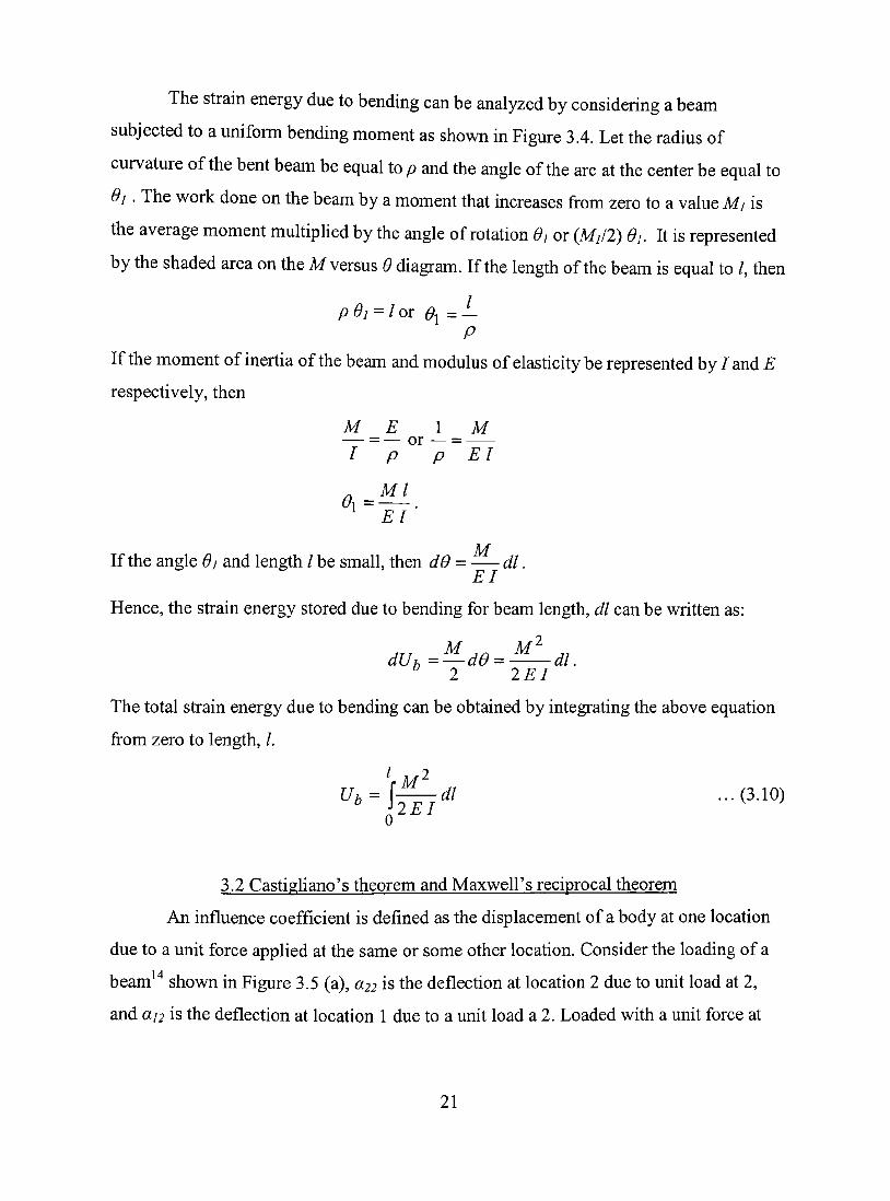
The strain energy due to bending can be analyzed by considering a beam

subjected to a uniform bending moment as shown in Figure 3.4. Let the radius of

curvature of the bent beam be equal to p and the angle of the arc at the center be equal to

di . The work done on the beam by a moment that increases from zero to a value Mj is

the average moment multiplied by the angle of rotation di or (M//2) ôi. It is represented

by the shaded area on the Mversus 9 diagram. If the length of the beam is equal to /, then

p6i = lox 6'i = — P

If the moment of inertia of the beam and modulus of elasticity be represented by / and E

respectively, then

M

/

sma

E = — or

P

Ml

EI •

11 thfin

1

P

ílf)

M

EI

M If the angle 61 and length / be small, then dÔ = dl.

EI Hence, the strain energy stored due to bending for beam length, dl can be written as:

M M^ dUu =—dø = ^^^dl.

^ 2 2EI

The total strain energy due to bending can be obtained by integrating the above equation

from zero to length, /.

^ M ^ Ut = ljjjdl ...(3.10)

0

3.2 CastigUano's theorem and MaxweU's reciprocal theorem

An influence coefficient is defined as the displacement of a body at one location

due to a unit force applied at the same or some other location. Consider the loading of a

beam " shown in Figure 3.5 (a), ^22 is the deflection at location 2 due to unit load at 2,

and aj2 is the deflection at location 1 due to a unit load a 2. Loaded with a unit force at

21

location 1, as in Figure 3.5 (b), the deflection at 1 is an and the deflection at 2 is a^,. The

value of the coefficient can be determined analytically or experimentally by applying a

load, measuring the corresponding deflection at the desired location and dividing

deflection by load. In Figure 3.5 (c), the same beam is loaded by forces Pi and P2 and the

"mfluence" of P^ on the deflection at location 1 is the product oíaijPj, etc. so that total

deflection at a given point is:

Vj = aiiPi + «12-^2 ^nd V2 = 0C2\Pi + «22-^2 (3.11)

ra) (b)

(0

Figure 3.5: Influence coefficients for beam deflections Source: A.H.Burr, J.B.Cheatham , Mechanical Analysis and Design,

(2" ^ Edition), 1999.

Two work sequences are used to prove the theorem of reciprocity. In Figure 3.6

(a), a force applied at location 1 is built up from zero to a value Pi, while doing the work

Pi{aiiPi)/2. This is foUowed by a buildup in P2, which does the work P2 {0.22^2)^2 at

location 2, while the constant force P/ moved through the distance anP^ and does the

work PiianP^). If there is no deflection at the supports, no work is done there.

22

«12^2 p 022^2 aiiPi P-, ^ ' ' ' 1 ^

Figure 3.6: Work done on a beam in sequence (a) and (b) Source: A.H.Burr, J.B.Cheatham^^ Mechanical Analysis andDesign.

(2"Êdition), 1999.

The total work done and the energy stored is given by:

U = ânPi^ +â22P2 +o^nPiP2-

In the sequence shown in Figure 3.6 (b), force P2 is applied first, doing work P2(0.22^2)12,

followed by Pj with work Pj(a]jPj)/2, and additional work by P2 of amount ^2(0.21^})-

The total work or energy stored is given by:

U = ânPi ^^cciiPi +^21^1^2 •

Since the fmal energy stored must be the same irrespective of the sequence used, from the

above two equations the condition then becomes that

a2j-aj2 ...(3.12)

23

This proves the theorem of reciprocity and states that, the deflection of a beam at location

2 due to unit load at location 1 is equal to the deflection at location 1 due to unit load at

location 2. This theorem applies to other loads and locations as well, and in general

o.mn=o.nm. It appUes uot ouly to beams, but to any elastic body.

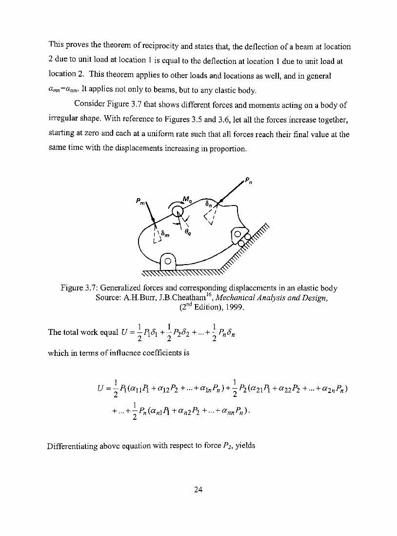
Consider Figure 3.7 that shows different forces and moments acting on a body of

irregular shape. With reference to Figures 3.5 and 3.6, let all the forces increase together,

starting at zero and each at a uniform rate such that all forces reach their fínal value at the

same time with the displacements increasing in proportion.

O

Figure 3.7: Generalized forces and corresponding displacements in an elastic body Source: A.H.Burr, J.B.Cheatham'^, Mechanical Analysis andDesign,

(2"* Edition), 1999.

The total work equal U = - Piî ^-P^S^ +... + -Pn^n

which in terms of influence coefficients is

U = -P\{anPi +a\2P2 +- + a\nP„) + -P2(a2\P\+a22P2+- + CX2nPn)

+ ... + -Pn(an\P\+an2P2+- + annPn)-

Differentiating above equation with respect to force P^, yields

24

dU 1 = T^1^12 +-(^21^1+2^22/^2 +-.. + ^2 .^« ) + - + ^^; .^«2 dP2 2 ' '"• 2 ^' ' --ll^l ^ln^n) — ^2

Applying the reciprocity theorem to above equation and adding the terms, we get

— = a2iPi+a22P2+--ÔC2nPn=S2

since the sum is by definition equal to the displacement at location 2. Generalizing this,

the CastigUano's theorem is obtained which states that, the partial derivatives of the total

strain energy in an elastic member or stmcture with respect to any of the extemal

"forces" is the "displacement" of the point of appUcation of that force in the direction of

the force. In equation form the theorem is written as:

. dU ^^ dU Sn =^—and^„ = . ...(3.13)

" dP^ dM^ ^ ^

This theorem can be used mainly in the analysis of curved beams and rings and also for

analysis of stmctures.

3.3 Forces Acting upon Bit and Bottom Hole Assembly (BHA)

A free-body diagram of a BHA section * between the bottom stabilizer and drill

bit in a vertical hole is shown in Figure 3.8. The centroidal axis of the BHA section is

assumed to be vertical at the point where the bottom stabilizer is placed. Below this point,

the BHA deflects slightly from the vertical axis die to the forces from drill bit and the

inertial force due to rotation of the drill collars. The reference axes x djxåy are within the

maximum deflection plane which is rotating at a circular frequency coy.

Forces acting upon the BHA section include forces from the stabilizer, drilling

fluid, gravity and drill bit. General forces acting upon the BHA section from the stabilizer

are axial force in the x-direction Fsx, shear force from stabilizer in j -direction Fsy,

25

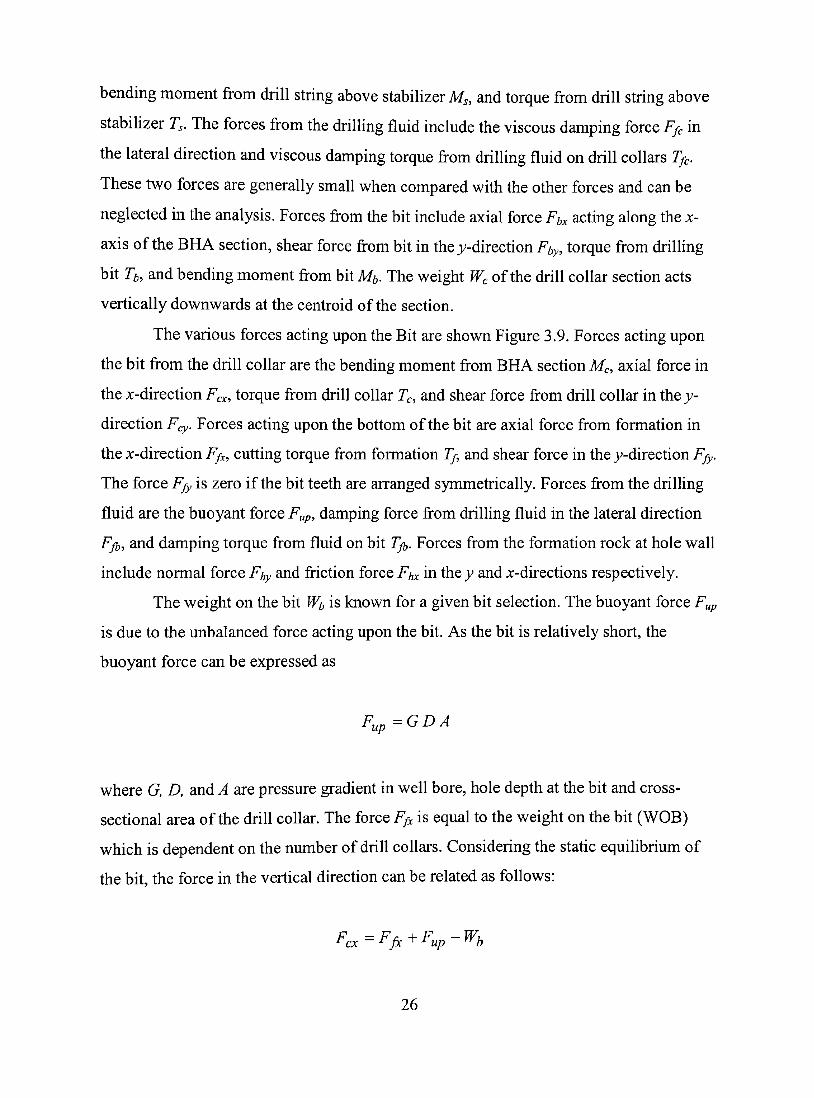
bending moment from drill string above stabilizer M„ and torque from drill string above

stabilizer T^. The forces from the drilling fluid include the viscous damping force / > in

the lateral direction and viscous damping torque from drilling fluid on drill coUars 7>.

These two forces are generally small when compared with the other forces and can be

neglected in the analysis. Forces from the bit include axial force Fb^ acting along the x-

axis of the BHA section, shear force from bit in the j^-direction Fby, torque from drilling

bit Tb, and bending moment from bit M . The weight Wc of the drill collar section acts

vertically downwards at the centroid of the section.

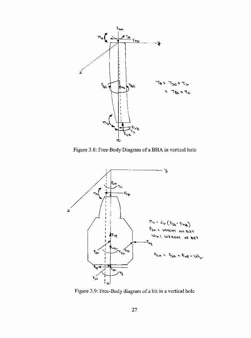
The various forces acting upon the Bit are shown Figure 3.9. Forces acting upon

the bit from the drill collar are the bending moment from BHA section Mc, axial force in

the x-direction Fcx-, torque from drill collar Tc, and shear force from driU coUar in the;^-

direction Fcy. Forces acting upon the bottom of the bit are axial force from formation in

the x-direction F^-, cutting torque from formation 7}, and shear force in the jv-direction Ffy.

The force Ffy is zero if the bit teeth are arranged symmetrically. Forces from the drilling

fluid are the buoyant force F„p, damping force from drilling fluid in the lateral direction

Ffb, and damping torque from fluid on bit Tfj. Forces from the formation rock at hole wall

include normal force Fhy and fiiction force Fhx in X\\cy and x-directions respectively.

The weight on the bit Wb is known for a given bit selection. The buoyant force Fup

is due to the unbalanced force acting upon the bit. As the bit is relatively short, the

buoyant force can be expressed as

Fup=GDA

where G, D, and A are pressure gradient in well bore, hole depth at the bit and cross-

sectional area of the drill coUar. The force / > is equal to the weight on the bit (WOB)

which is dependent on the number of drill collars. Considering the static equilibrium of

the bit, the force in the vertical direction can be related as follows:

Fcx=Ffx+F^p-Wj,

26

/

c ^bf - ^

F

rn ^í

- = ^ ^^V

V

Figure 3.8: Free-Body Diagram of a BHA in vertical hole

î5<- ^ V M ^ " Vj i M ^ - v y i ^

Figure 3.9: Free-Body diagram of a bit in a vertical hole

27

The formation reactions 7/and Ffy can be calculated from analysis of the PDC bit

force model presented in Chapter 2. The vertical and horizontal cutting force components

from equations 2.4 and 2.6 can be written as:

2SsA^cos(T-a) Fv= ; \ ^' / ...(3.14)

1 - sm(r - a)

F^JS,A,sm(r-a) ^^^^^

1 - sin(r - a)

2 where area of the cut, Ac= Or - r(r - ô) sin O

0 = cos"M 1 V r J

and ô = cutting depth

r = radius of cutting blank.

The cutting torque from the formation consists of two components: cutting torque

generated by the horizontal cutting forces and friction torques generated by the vertical

cutting forces. The average value of the cutting torque can be expressed as

Tfa=XRiF^,^Y./'F,,R, . ...(3.16) i=l i=l

where ju is the friction coefficient between the cutter and rock. If the bit does not vibrate

laterally, 7/wiU be constant and equal to 7} . The lateral vibration of the bit in the x-y

plane may result in a harmonic variation of the resultant torque 7/. Therefore, 7/can be

expressed as

Tf=Tf^+Tf„sm{coit) ....(3.17)

28

where 7} is the fluctuation in cutting torque from formation, COL is the circular frequency

of lateral vibration in the x-y plane. The maximum amplitude of the fluctuation can be

expressed as

^ fo = ^ f max ~ ^ fa

where the maximum torque Tfmax may depend on several factors such as weight on bit,

rotary speed, rock properties, and tilt angle of the bit, etc.

The resultant lateral force 7y also consists of two parts: total cutting force

generated by horizontal cutting forces and friction forces generated by the vertical cutting

forces.

Ff=f,(FH)i^f,pi(F,)i ...(3.18) i=\ i=\

If the cutters are arranged symmetrically in the bit face, both of these two sums are equal

to zero. Otherwise, the resultant force F/has a non-zero magnitude and a changing

direction because of the relative rotation of the bit with respect to the rotating x-y plane.

Therefore, its major component in the j^-direction, F^, can be expressed as:

Ffy = Fjya ^Ffy^ sin(co,t) ... (3.19)

where cor represents the angular velocity of the bit relative to the wobbling plane, Ffyo is

the fluctuating amplitude of the resultant cutting force in the >'-direction and can be

expressed as

^ fyo = ^ fymsíx ~ fya

and Ffymax^^y again depend upon several factors including weight on bit, rotary speed

and tilt angle of the bit. If the force F/does not act through the center of the bit face, it

also exerts a torque on the bit. This torque is assumed to be negligible in the analysis.

29

The lateral force Fhy is due to the hole-wall contacting the bit. Its magnitude

depends on lateral displacement of the bit and properties of the hole-wall rock. This force

generates additional stresses in the neighborhood of the contact area^^. The average

normal rock stress induced by the force Fhy may be approximately expressed as:

C T ; - ^ . . . ( 3 .20 )

The average normal strain over the contact area may be expressed as:

^r~r[^ø-^^z\ ^r = Er'

CT,

Er ...(3.21)

where aø and a^ are the tangential and the axial stress in the formation due to the bit

impact.

The deformation of hole-wall rock at the contact area is equal to the lateral

displacement (y^) of the bit. líDr is defined as the effective lateral depth within which the

in-situ rock stress is altered due to the bit contact, then the average normal strain Sy. can

be approximated as:

s , ^ ^ . ...(3.22) D ^r

Substitution of equations 3.20 and 3.22 into equation 3.21 yields:

F^y=E,A,^. ...(3.23)

The tangential fiiction force is given by:

Fhx=l^hv - (^ -^^)

30

The damping force Fy& and damping torque 7}z, are given by:

Ffh =Cf^L ...(3.25)

and Tfl,=c,DÂ,Tdf ...(3.26)

where v/,, Db, A^ and r^/ represent the lateral velocity, bit diameter, bit surface area, and

shear stress of the drilling fluid, respectively. The viscous damping coefficients c/and C/

are difficult to determine analytically. However, since their values are very small and

negligible when compared to other forces, they are not taken into account in the analysis.

The lateral force from the drill coUar Fcy is the reaction force oíFt,y which can be

determined from the deflection analysis considered later in this chapter. The torque Tc

from the drill collar is the reaction torque of T and can be written as:

T,=T,-Tf,. ...(3.27)

The fiiction force from the well-bore Fhx generates a fiictional torque which can be

estimated as Fhx Di/2. The bending moment M^ from the drill collar can be expressed as

M,=Lj,(Ffy-Fhy) ...(3.28)

where L^ is the length of the bit and the damping force from the drilling fluid, Ffj, is

neglected. Since Lj, is smaU compared to the length of drill coUar, Mc is small and

negligible.

3.4 Elastic Constants of Bottom Hole Assembly

3.4.1 Static Conditions

If the BHA section shown in Figure 3.8 is stationary, the BHA can be analyzed as

a beam hung in a vertical hole. Then the force Ffc and torque 7} are equal to zero as there

31

is no rotation. The bending moment Mj, is negligible because the length of bit is small

compared to that of the BHA section. Then, the linear relationship between the lateral

force Fby and lateral deflection j^^ can be estabUshed. The linear relationship between the

torque Tb and angular deflection OL can also be established. The proportionality

coefficients in these relations are called the elastic constants.

The total elastic strain energy U in the BHA section is determined by adding the

terms giving the energy accompanying the work done by a bending moment, direct shear,

axial force, and torsional load:

U = Uj,+UsÛa+Ut ... (3.29)

where Ub, Ua, and Ut are the strain energies due to bending moment, axial load and

torsional load, respectively.

The bending moment in the BHA section is approximately given by:

M. M,=Fj,y(L-x)^^{L-x)

= {L-x}F, by (3.30)

where L is the length of the beam (BHA assembly) and x is the distance with reference to

the lowest stabilizer.

Substituting equation 3.30 into equation 3.10 gives:

L{L-X)-

Ub = \ 0

Fby + M,

2E,I, -dx

where Er and L are the elastic modulus and area moment of inertia of the driU collar.

32

6^c4 Fby +

M,

Neglecting the small value oíMblL

Ub = ÛFI

Ê,I, (3.31)

The shear stress in the BHA section can be approximated by:

xy ^ ^^y

A (3.32)

From equation 3.7 considering shear force acting on only a single plane, the strain energy

stored in an elemental length dx is given by:

U^ ^—xr^xS^xAxdx . (3.33)

where js is the shear strain and Ss is the shear stress.

1 5 U. =—x—^xAxdx

' 2 G ... from equation 3.2

C/.=^xí<lMx^.rf, from equation3.3

Pby(^ + r)

AE. dx. .. (3.34)

33

The total strain energy can be obtained by integrating equation 3.34 from 0 to L.

KFÎ (1 + y) U,= p ^ — ^

= -^ ...(3.35) E,A

Since the gravitational force is uniformly distributed along the length of the BHA

section, the axial force can be expressed as:

Ta=w{L-x)-Ft,^ ...(3.36)

where w represents the unit weight of the drill coUars and Fbx approximately equals:

Fj^^GDA. ...(3.37)

From equation 3.8 considering force acting only in the axial direction:

U a =—xaxsx Axx

where a and s are represent the axial stress and the axial strain.

Aax 2E,

Dividing equation 3.36 by area A gives the axial stress a which upon substitution in

above equation and integrating from the limits OtoL gives the total strain energy stored

due to the axial force.

0 '^

34

î— j[w^ {L - x)2 + {GDA)^ - 2w{GDÃÍL - x))^ 2E,A

L

2E,A

0

2 r 2 w L

3 + {GDAY -{GDA)WL ...(3.38)

From equation 3.9 for strain energy stored due to torsional load, we get

U,= sj (DI+DI) 4G D}

2 /T^2 . 7^2 ^ ( D | ^ ^ . ( 2_ 2^ 4G /)2 4W ir-

5f 2 Í±dx^(Di-Df)b^ 4 £ ^ D | 4

LQ 'JZ

dx (3.39)

where J^ is the polar moment of inertia and is defmed by

32

At any radms ic, — ^ R

-Tb

Jz

Integrating equation 3.39 from 0 to L yields:

Ut-\^ 0 ^^'^^

T^L{\ + r)

Ec Jz

dx

(3.40)

35

The total energy Uis obtained by substituting equations 3.31, 3.35, 3.38, and 3.41 into

equation3.29.

^^^^^âf^,_A 6EJ, EÂ 2EcA

2j2 w L + {GDAf -{GDA)WL +

T^L{\ + r)

Ec ^ z . (3.41)

From CastigUano's theorem (equation 3.13), differentiation equation 3.41 with respect to

Fby and Tb gives the lateral deflection yi and angular deflection 6L, respectively.

yi dU

ÔF by

Û 2{\ + r)L Ê,L, EcA

F by ...(3.42)

û, dU

dTb

2{i + r)L Ec Jz

(3.43)

Equations 3.42 and 3.43 can be written as:

Fbv = ksyi ly ..(3.44)

Fh = e ^L ...(3.45)

where ks is defmed as the elastic constant for lateral deflection and ke is defined as the

elastic constant for angular deflection.

ks = L^ , 2{\ + r)L

3E,I, EcA ...(3.46)

36

ke= ^'^^ 2{\ + r)L

(3.47)

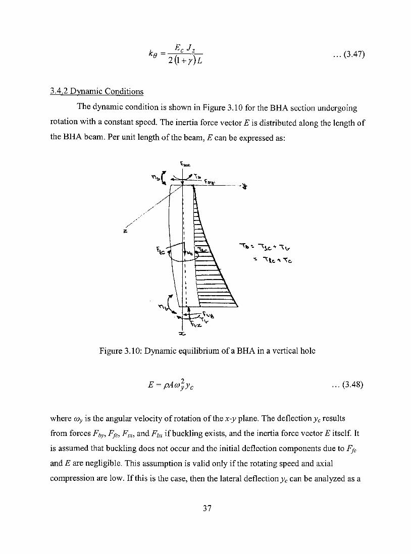
3.4.2 Dvnamic Conditions

The dynamic condition is shown in Figure 3.10 for the BHA section undergoing

rotation with a constant speed. The inertia force vector E is distributed along the length of

the BHA beam. Per unit length of the beam, E can be expressed as:

2.

Figure 3.10: Dynamic equilibrium of a BHA in a vertical hole

E = pAcOyy y.rc

...(3.48)

where coy is the angular velocity of rotation of the x-y plane. The deflectionjVc results

from forces Fby, Ffc, Fsx, and Fbx if buckling exists, and the inertia force vector E itself It

is assumed that buckling does not occur and the initial deflection components due to Ffc

and E are negligible. This assumption is vaUd only if the rotating speed and axial

compression are low. If this is the case, then the lateral deflection _yc can be analyzed as a

37

cantilever beam with a fixed load Fby at the free end of the cantilever. Consider a

cantilever beam of length L and having a concentrated load F^y as shown in Figure 3.11

C / ^ / / / /

^v

Figure 3.11: Cantilever beam with an end load

The differential equation for this type of loading can be written as

EcIz^ = Fby{L-x) dx^ ^

(3.49)

The two boundary conditions are as follows:

Atx = 0; dy/dx = 0

Atx = 0;y = 0 .

Integrating equation 3.49 once with respect to x, we get:

d ^ Ec^z -— = FbyLx^Fby^ + cx

where cj is the constant of integration.

Applying the first boundary condition the value oícj is equal to zero,

EÎ^ — = Fu^Xx - Fu., — c^ z dx

byJ^X Fby (3.50)

38

hitegrating equation 3.50 with respect to x, we get:

2 3 EcIzy = FbyL^~Fby^ + C2 ...(3.51)

where c^ is the constant of integration.

Applying the second boundary condition, the value of Q obtained is equal to zero. Hence

2 3 EcIzy^FbyL^-Fby—-

FbyX^{3L-x) y = y c = ^ ^ , • ...(3.52)

Ech

Substituting equation 3.52 into equation 3.48, we get

2 Fi,yX^{3L-x) E = pAco y Eclz

E = CnFb.x^{3L-x) ...(3.53)

pAû)l where C„ = ~.

6E,L,

If the damping force from the drilling fluid is negligible, then the bending moment in the

beam is generated by Fby and E.

Mz =M^f~\-M^^

The inertia force vector E generates a bending moment Mze at x as shown in Figure 3.11

and its magnitude equals

L

^ze = \^ E dx

= \x Cn Fby X \3L-x)dx .

39

Since X =X-xãnddx =dX, the above equationbecomes

L Mze = JC« Fby X^ {X-x){3L-x)dX

— ^n^by 3L + x)

V ^ ; L'-X']=XL{L'-X'

^Û-x'^

Strain energy due to bending is given by:

1 ^ Uu = \MI dx

2EJ. J " •c-z 0

L

C Z Q

..(3.54)

Substituting M^f = Ffjy {L - x) and equation 3.54 into above equation, we get

U, =.^Cn^ F} Û' +1 ÍC„ F 2 L ' + 1 F 2 Û . " 34650 ^y 35 " ^y 3 ^^

...(3.55)

From Castigliano's theorem:

yi = dU dUh Fhy

SFby dFhy

yi = kdFby

Eclz

U 11 ^ ,7 2641 ^2 r\\ + —Cy,L' +

3 35 " 34650 CtV

(3.56)

where Â: = 'û_

3

11 + —

35 Cn

Eclz

n 2641 L +

34650

C^ ^n

û'

and is defined as the dynamic elastic constant for lateral deflection.

40

3.5 Formulation of Bit Vibrations

3.5.1 Lateral Vibrations

The bit is treated as a particle without any mass in the lateral motion. The

equation of motion is applied in the >;-direction and the following relation is obtained:

Fjy -Fcy -Fhy -(Ff,)y = m dt^

. . .(3.57)

From equation 3.19, ignoring the small value oíFfya, Ffy « Ffy^ sm((Oyt) and

substituting equatíon 3.56, 3.23 and 3.25 into equation 3.57, we get

FfyoSm{co,t)-kdyi- yi-cf dyi „d yi dt m

dt (3.58)

d yi I ^ / dyi ,

dt^ w dt

EÂ ' '- + k.

V L > , F.

m yi = ^sm{cûrt)

m

where Fo = F, fyo-

andZ) = — , the above equation becomes

£ ) ^ + — i ) + (co^f yi=-^sin{(s>y.t). m m

..(3.59)

As the right hand side of equation 3.59 is not equal to zero, its complete solution equals

the sum of the complementary solution and the particular integral.

Equating the left hand side of equation 3,59 to zero, the equation is quadratic and

its solution is given by:

41

1+ r / Ê.A.^k^D,

D = m m Dj.m

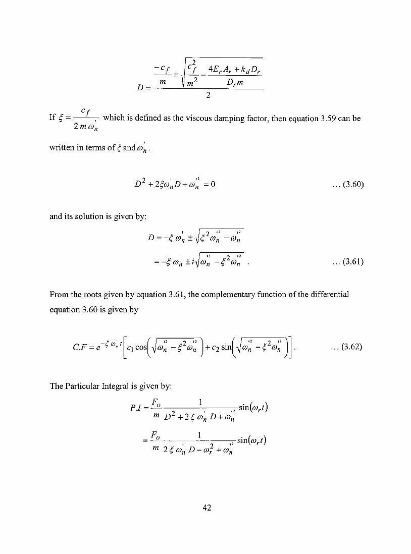
Cf If ^ = r which is defined as the viscous damping factor, then equation 3.59 can be

2mo)y^

written in terms of £, and «„ .

Z)^+2^íy„£) + íy„ =0 ..(3.60)

and its solution is given by:

Z) = - ^ íy„±V^ COn - « n

= -4(0^+1^0)^ -^ (Û„ (3.61)

From the roots given by equation 3.61, the complementary fimction of the differential

equation 3.60 is given by

C.F = e -^<t C\ cos læl -^^cû^ +C2SÍnU/ íy„ - ^ íy„ ...(3.62)

The Particular Integral is given by:

F P.I = ^

1 m r\2

— sm{co,t) D +2i^co„ D + a)„

1

f" 2^co'„D- )^ + col sm {co,t)

42

_Fo \o)y, -co'i]-24ú)^D

co^ -CD^j -4^ô)^ D^ sm {cD^t)

FQ K -C0r]-2^C0nD

m ( '^ 2V . ^2 " 2 û)^ -û)f. j -\-4g ú)^ øj.

\n{o)^t) sm

m 0) n -^rf 2 '2 2

+ 4 ^ 0)j^ 0)y.

o)jj - o)j. Isin(í2>^r)- 2 ^ û)yj o)y. cos{p)y.t)

If Rcosû = o)yj -øj. 2 ' /í ' 2 1 2 ' 2 y. dinåRsinØ = 2ô)yô)j.,ih.cn R = ^\^^ -^rj + 4 ^ 0)^^ æ^. .

Substituting the value of 7? in the above equation, we get:

F P.I = —^ [sin(íy^r)cos 6 - cos(íy^/)sin 6\

mR

i2 2 r 2 ' 2 m^j\o)f^ -o)j.] + 4 ^ o)y^ cOy

FQ s\n{p)y.t-6)

s\n{o)yt-0)

s\n{cOy.t-6)

cOy^m. 1 _ J ^

V ^n j

2ô)y

\ ^n J

fyo EyAy

+ A:.

sm ^ 2 ^

^ i2

2 / {co^t-û)

+ 2^co,

V ^n y

= 7/, sin(íy^í - d) (3.63)

43

^ fyo where Y^ = D.

and tan 6 = A2

l_f^ Cú

+ n J

f \2 2^C0.

\ ^n j

2^0)y,CO,

CÚfJ — COy.

OT 6 = tan 2^0) yjO)^

^n 0) r J

The term YL is the constant amplitude term and is the steady state amplitude. The

complete solution of the differential equation 3.59 is the sum of equations 3.62 and 3.63

The constants defmed in equation 3.62 need to be determined based on the boundary

conditions given by:

At/ = 0;j^/,=jîoand

At dyL dt

t=o = ô where Vo is the initial linear velocity of the bit.

Applying the first boundary condition to equation 3.62, we get

yLo =<^l=>c\= VLO '

Differentiating equation 3.62 with respect to t, we get

•^^-ía^ê-i".-dt

• : ) cj coslíy^ -(^ o)j^ r + c^sinlíy^ -^ æ c)i +

•ô)'t V \2 2 ' í / ~^ 2 ^ íy„ - ^ íy„ sin - íy„ - ^ co^ t + C2Í03n - ^ 0)n COS ^^(Oj, -£, « „

Applying the second boundary condition to the above equation, we get

dyi dt

=^=^0= - # 0)n C\ + C2 ^C n - ^ ^ ^ «

|2 2 '2

C2

C2

ô+^(^n yu

CO, n ^ 0)n

ô^ + ^) ô-l^ ^c

co ;Vw^ íy«Vw CÛ,

AA

with the assumption that ^(l + )/(l - ^) »1 as (f is very small.

Lci o)^=o)j^ - ^ ^ ^ « =>o)^ =o)yj^j\-<^'^ . (3.64)

The term o)d in the above equation is defined as the damped pseudo-natural frequency.

Substituting the values of cy and c^ in equation 3.62 and writing the final solution by

adding equations 3.62 and 3.63, we get

yL=^ •^<j yio cos{o)^t)-\-^sin{o)^t)

= j3Îo + \<^n /

-í^:^ L

ylo^ í \

\^nj

V, yj^^cos{co^t)^^s\n{cOdt)

0)^

Let C = J : ío + r \

\^n j

, then the above equation becomes

yf^^Ce ^^^^[sin^^cos((5;^r)+cos^sin(íy^r)] =Ce ^^"^ s\n{a)^t^\ij)

where sin \f/ = yLo ,COSl//

O^ 0)yj

^' " and^ = tan

ylo^ ( \

Or.

\^n j ylo^

r \2 o.

\^nj

í ' \ yLo^n

ô \ ^ J

The final solution for the lateral deflection of the bit is given by

yi=Ce~^"^" ^ sin{o)dt)^YL sin^Wyt-6). (3.65)

Neglecting the transient state solution of equation 3.65, the steady state part of equation

3.65 gives the lateral displacement of the bit and is expressed as:

45

yi = YL sm{(o^t - e) ...(3.66)

As 0)j. approaches ty^, resonance occurs. Near resonance the magnitude Yi of the

steady-state solution is a strong function of the viscous damping factor ^ and the non-

dimensional frequency ratio y / íy„ . Under the resonance condition, the bit wobble

causes the early failure of the PDC bit. The critical 0)r that causes resonance can be

determined using the following equation:

k^ + '^ ^ D,

COj. = (3.67) m

where kd is defmed by equation 3.56

Since the term kd is very small, it can be neglected in the above equation. The

condition at resonance, then becomes

0)y = Ef.Ay

Dj.m ..(3.68)

The amplitude at resonance can be determined by substituting co^ = «„ in the term YL of

equation 3.63.

'fyo YT =

Ê A ^ n

..(3.69)

1 _ _ ^

V ®« y +

2>^

V ^« y

The denominator of above equation equals 2, and the amplitude Yi at resonance equals

Ffyog, ^ f- 2 2go)j-m

where, gc is the gravitational constant for the following units;

46

Ffyo =M Ay. =in^

kd = Ibflft D, = in

Ej. = psi

The time period at resonance equals ^njcûj.

3.5.2 Angular Vibrations

For a drill bit under penetrating condition, the un-balanced lateral forces acting

upon the bit will cause a lateral vibration of the bit in a maximum deflection plane (x-_y

plane). The unbalanced torsional loads result in the angular vibration of the bit. The bit is

treated as a particle in the lateral motion and equation of motion is applied in the j ^ -

direction which yields the following differential equation:

Tc-Tjb-Tf-Fhz^ = I m . ^ -(S.VO)

where:

Fc =Ts -Tfc =Tb

Tf=Tf^+TfoSÍn{o)Lt)

Fhz = M Fhy

Substitutíng the above equations in equation 3.70, we get

2 Fh Du d 6 Ts -Tfc -Tfb -Tfa -Tf,ún{coLt)-^^:^ = Imx—f - ^ - ^^

But we have from the relation: T^ = Tf^ + Tf^ + Tfb

Substituting this relation into equation 3.71, we get

2

r , „ s i „ K , ) - ^ í ^ n = / » . ^ -("2) Ê), dt^

47

Considering only the steady state component ofyi, we get

yi ^YiSÍn{o)j.t).

Substituting above equation into equation 3.72, we get

2 -Tf,sm{o),t)-^Í^^Y,sm{a),t)=I^^^^ . ... (3.73)

^^r dt

T rr. jUDuEj.Aj.

Leti^ = Yi, then equation 3.73 becomes: r

d^6, TfoSÍn{o)i^t)-T^sin{o)j.t) = Ijj,^ -^ . ... (3.74)

dt^

Equation 3.74 is the goveming differential equation of the angular motion of the bit in the

x-y plane.

Integration equation 3.74 with respect to time t, we get

— ^ = —^^cos{o)j.t)-\-—^^cos{o)f.t)-^C2 ... (3.75) at COj. 1 yj^j^ 0)j. 1 jyij^

where cs is the constant of integration.

dØ Att = 0 — ^ = 0)^, where coo is the initial angular velocity of the bit.

dt

Substituting this boundary condition into equation 3.75, we get:

Tfo + T^ Tfy + T^ 0^0 = ~ ^ + ^3 ^ ^ 3 =^0 j

d6j Tfy + r^ \ Lfo+ T^ — ^ = 0) = 0)^ -\-— cos(íy^/j .

at o)j. 1 jj^-^ o)j. 1 ^-jj-

Considering the absolute angular velocity, we get

48

Tr -[-T o) = o)r.^ — [1 - cos(íy^ t)\

0)j,I mx

(3.76)

Integrating equation 3.76 with respect to time t, we get

OL =û>ot + ^ ^ ^r^mx

sm {o),t)

co. + C4 (3.77)

At /=0 <9i = 0 => C4 = 0

Hence equation 3.77 becomes

QL =o)ot + Tfo + T^

^r^mx

\n{o)f.t) sm 0),

...(3.78)

The angular velocity and angular displacement of the bit motion due to the un-balanced

torsional loads are given by equations 3.76 and 3.78, respectively.

49

CHAPTER 4

BIT WOBBLING-CALCULATIONS, RESULTS AND DISCUSSION

4.1 Examnle Calculations

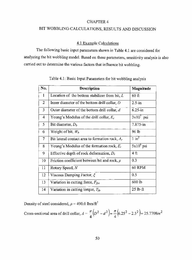
The following basic input parameters shown in Table 4.1 are considered for

analyzing the bit wobbling model. Based on these parameters, sensitivity analysis is also

carried out to determine the various factors that influence bit wobbling.

Table 4.1: Basic Input Parameters for bit wobbling analysis

No.

1

2

3

4

5

6

7

8

9

10

11

12

13

14

Descriptioii

Location of the bottom stabihzer from bit, L

friner diameter of the bottom drill collar, D

Outer diameter of the bottom drill collar, d

Young's Modulus of the drill coUar, Ec

Bit diameter, D/,

Weightofbit, Wb

Bit lateral contact area to formation rock, Ar

Young's Modulus of the formation rock, Er

Effective depth of rock deformation, Dr

Friction coeffícient between bit and rock, ^

Rotary Speed, A'

Viscous Damping Factor, ^

Variation in cutting force, Ffyo

Variation in cutting torque, Tfa

Magnitude

60 ft

2.5-in

6.25-in

3x10' psi

7.875-in

96 Ib

lin^

5x10''psi

4ft

0.3

60RPM

0.5

600 Ib

25 Ib-ft

Density of steel considered, p = 490.0 Ibm/ft

Cross-sectional areaof drill coIlar,/í = - ( D ^ -d^]= -(6.25^ -2 .5^ )= 25.7708/«^

50

T V 1 1 1 • . 2nN 2 X ; T X 6 0

Initial angular velocity = o)o= = = 6.2832 rad/sec. 60 60

AreaMomentoflnertia, /^ =—(D^-^"^1=—(6.25^-2 .5"^)—/? '^ = 0.0035197//"^. 64 ^ ^ 64 ^ ^12^

From equation 3.53; C„ = T";;—~ft 6E,I,

Writing the above equation in terms of individual units, we get

^n

pAcol i ^ . - V . . 2 V , A

6 c ^z 6

Ibm

yfi j

fi 144,

V J vsec j

1 1

^ Ibf 144^

fi 2 1 /^'

V. / " J

1 1 Ibm \

6 144^ /6/ / í^ sec^ ^c 6 x 144^ x 32.2 ^ /r"^ =2.496134 X10"^/r"^

Hence,C„ = 2.496134x10"^ x ^ft'^ ' ^« 6Æc/z

...(4.1)

Substituting the known values into equation 4.1, we get

3x10^x0.0035197

From equation 3.56, k^ = EJz

3 35 " 34650 "

51

If the units ofEc, L, Cn, and L are psi,ft'',ft'\ andft, respectively, and the unit of rf is

Ibf/ft, then

k^=^

3

11 + —

35

\44EJ,

" 34650 C^ ^n

û' Ibflft (4.2)

Substituting the given values in kd, we get

kd 144x3x10' xO.0035197

60 +

3 35 — 1.178x10-^ x 6 0 ^ + ^ ^ ( l . 1 7 8 x 1 0 - ^ ^ x 6 0 ^ ^

34650

= 3.0721 Ibflft

Fromíy„ = checking for the units, we get

Ibf Ibm ft Ibm ft ibf sec^ sec

deglsec. (4.3)

Substituting the given values in above equation, we get

^5x10^x1

(y,

+ 3.0721

96

x32.2

= 647.5 deglsec^ 11.301 radlsec.

52

The viscous damping factor is dimensionless and is given by < = ——;- . Writing this 2 m 0):

equation in terms of individual units, we get

^f _ Ibf -scc \ 1 _lbf - sec Ibm ft f 2 m íy„ ft Ibm í 1 A 1 \ Ibmft Ibf-scc^ ImcOyj

^sec^

rx<?-

2mo)r. ..(4.4)

From the given data, the value of <f is equal to 0.5

'fyo At resonance, Y^ =

Ej.Aj.

\ ~ ^ -\-k.

2# from equation 3.63

Substituting the given values in above equation, we get

'fi'O Yj =

Ej.Ay + k. 600/

^5x10^x1 3.0721

U 2x0.5 = 4.8 x l O " V = 0.00576/«.

2£cû„C0r ^ n From tan 6 = ,, , at resonance d = —

COyi -cOy ^

Substituting the values of YL and 6 in the steady state term of equation 3.65, we get the

following relation

...(4.5) Yi = 0.00576 xsin 641.5t 2

53

The mass moment of inertia, Imx assuming the bit as a sphere is given by:

lyy,^ =~Ma^ =-mD^ = - x 9 6 x - ^ = 4.\34 Ibmft^ 5 5 ^ 5 144x4 ^

_ _ juDi.Ej.Aj. ^^ tvom 1^= — — Yi, writmg m terms of individual units, we get

T =

r Ibf , 2 ftx^^xin

'^^ ^ft=lbfft

Rcncc. T.,=^^^^^Y,ft ' -"w 2D,

(4.6)

Substituting the individual values in T^, we get

x 4.8x10 = 59.0625 Ibfft 0 . 3 x ^ ^ x 5 x 1 0 ^ x 1

T = 12 2x4

From equation 3.76, we have

6i =o)^t + Tfo +^w

^r^mx t-

m{o)y.t) sm 0),

(4.7)

Each term in the right hand side of equation 4.7 should be dimensionless. Considering the

dimensions of the second term in the above equation we get:

Ibf-ft 1 Ibf-scc^ •^ X — X sec = —

f—1 ^secy

Ibm- ft Ibm - ft

54

http://juDi.Ej.Aj

Introducing the gravitational constant, gc in the above equation we get:

Ibf - sec Ibf - sec Ibm - ft ~Ti T~ ^gc = ~ — X T = dimensionless

Ibm-ft Ibm-ft ibf-sQC^

Hence equation 4.7 re-arranged with the proper units becomes:

6i =o)ot-\-^Tfo -\-T^^

\ ^r^mx j g<

sm {o),t) 0),

. . .(4.8)

Substituting the given values in equation 4.8, we get:

(25 + 59.0625)x32.2 6J =2nt-^ '-

647.5x4.134

t sin(647.5/) 647.5 ^

= 6.2832í-17.7622 í-1.5444xl0"-'sm in(647.5r)J. • (4.9)

4.2 Results and Discussíon

From equation 3.63, it is observed that resonance occurs when the firequency ratio

\^y. IcOyj I is equal to unit in the Yi term. Using equation 3.66 and substituting the values,

the lateral displacement of the bit is plotted with time as the parameter under resonance

condition. The corresponding data for all the figures shown in this section is enclosed in

Appendix A. The path of the bit center is shown in Figure 4.1. The plot indicates that the

bit undergoes a wobbling motion. As a result of this motion, a lobed pattem of the bottom

hole is observed when resonance occurs. The maximum amplitude of vibration at

resonance is calculated to be 0.00576-zn for the given conditions. For non-resonance

conditions, Figures 4.2 and 4.3 indicate the path of bit center for frequency ratios of less

than one and greater than one, respectively.

55

0.008

•O.OOB o.ooa

•0.008

Figure 4.1: Path of bit center at resonance condition

Figure 4.2: Path of bit center at non-resonance condition (Frequency ratio=0.88)

56

. oa

-0.008-

Figure 4.3: Path of bit center at non-resonance condition (Frequency ratio=1.30)

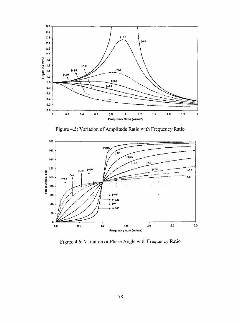
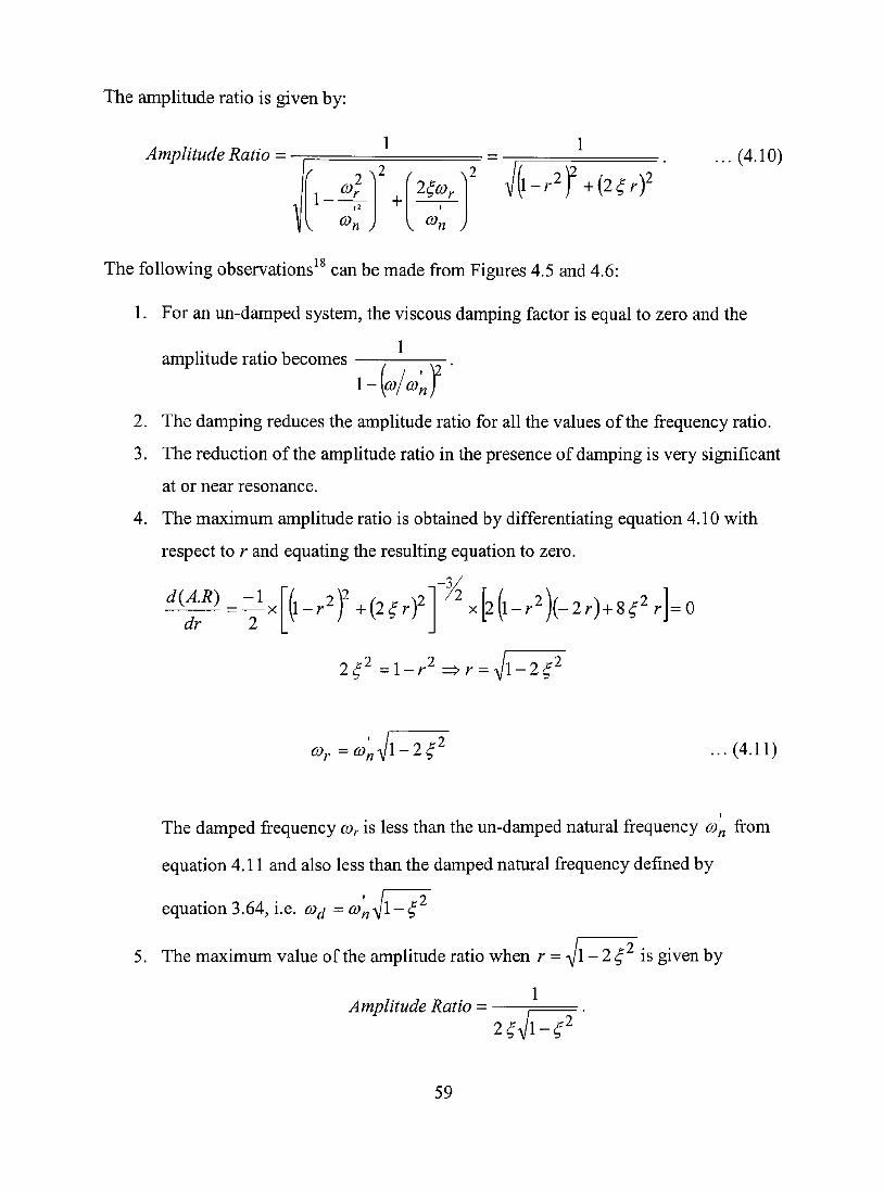
The effect of lateral vibration amplitude with fi'equency ratio for a given viscous

damping factor is shown in Figure 4.4. Figure 4.5 shows the variation of amplitude ratio

(ratio of the observed amplitude to the amplitude at resonance condition) with frequency

ratio. The variation of phase angle with frequency ratio and damping factor is shown in

Figure 4.6.

0.4 0.6 0.8 1 1.2

FrequAncy Ratio (wr/Wn*)

1.4

Figure 4.4: Variation of AmpUtude with Frequency Ratio

57

2.8 -

2 .8 -

2 .4-

2 5

2 .0 -o

e l^ • ro tE:

« 1.6 -•u Í 1.4-tL

1 1^^ 1.0 -

0.8 -

0.6 -

OA '

0,2 -

0.0 -

t=2JÍ

— , — , j —

M.6

í-1.0

— 1

/ í " 0 .2

-- -^ .^ .^ . lEÔ.O^^ ' ' * "* ' ' ' ' *^ , , , , . .^

"-"fc..^.^^^^^^ • • * « * • ,

s.

\ Í-O.D

' ^ ' " • - • - ^ ' ^ ^ ^ ^ N ^

^ ^ ^

0.2 0.4 0.6 0.8 1 15

Frequency Ratio (wrAn/n*) 1.4 1.6 1.8

Figure 4.5: Variation of Amplitude Ratio with Frequency Ratio

180

160 •

0.0 0.5 1.0 1Æ 2.0 Fre<|uency ratio (wr/wn')

Figure 4.6: Variation of Phase Angle with Frequency Ratio

58

The amplitude ratio is given by:

Amplitude Ratio =

1 _ ^ 2 ^2 / A

V ^n j +

2^co,

K ^n j

(l-r^f+(2^ry . (4.10)

The foUowing observations^^ can be made from Figures 4.5 and 4.6:

1. For an un-damped system, the viscous damping factor is equal to zero and the

amplitude ratio becomes —-. —-.

2. The damping reduces the amplitude ratio for all the values of the frequency ratio.

3. The reduction of the amplitude ratio in the presence of damping is very significant

at or near resonance.

4. The maximum amplitude ratio is obtained by differentiating equation 4.10 with

respect to r and equating the resulting equation to zero.

-3/ d(A.R) - 1 —^ = — X

dr 2

[\-r^J+{2^rf 2\\-r ) ( -2 r ) + 8 # ^ r = 0

2^^ = 1 - / - ^ ^r = Vl-2^'

0). = co'J\-2^^ ...(4.11)

The damped frequency Or is less than the un-damped natural frequency o)y^ from

equation 4.11 and also less than the damped natural frequency defined by

equation 3.64, i.e. o)^ =o)yj^j\-<^

5. The maximum value of the ampUtude ratio when r = -yl - 2 is given by

1 Amplitude Ratio =

4 ^

59

The above equation can be used to determine the amount of damping present in a

system if the maximum amplitude of the response is measured. Conversely, if the

magnitude of damping in a system is known, an estimate of the maximum

amplitude of vibration can be made.

6. Below resonance, the phase angle increases with increase in damping. Above

resonance, the phase angle decreases with increase in damping.

Brett et al. concluded that the failure of PDC cutters in hard rock drilling is due

to cutter chipping (impacts from vibrations). Cutter chipping occurs when the cutter

moves backward due to bit wobbling. Figure 4.7 shows the schematic of the bit face. The

wobbling motion of the bit in the bit-face plane can be resolved into two motions, i.e.,

lateral and rotational motion. hi Figure 4.7, thick arrows represent cutter velocities in the

lateral motion of the bit, while thin arrows represent cutter velocities in the rotational

motion of the bit. The vector sum of velocities due to these two motions is the total

velocity of the cutter. At points B, C, and D, the magnitudes of the total velocities are

greater than the magnitudes of their component velocities. At point^, the magnitude of

the total velocity is less than that of its component velocities. The cutter velocity at point

A can either be a forward velocity or be a backward velocity depending upon the

magnitude of the velocities due to the lateral and rotational motion. If the magnitude of

the velocity due to lateral motion is greater than that of the velocity due to rotation, the

cutter at point A will have a backward velocity. This backward velocity may cause cutter

chipping if the formation rock is hard.

Taking derivative of the steady state part of equation 3.65, the lateral velocity of

the bit center is obtained and given by:

Vc = h ^r cos{o)j.t-(^). ... (4.12)

The rotational velocity of the cutter at a distance rl from the bit center is given by:

Vryc=co^ . . .(4.13)

60

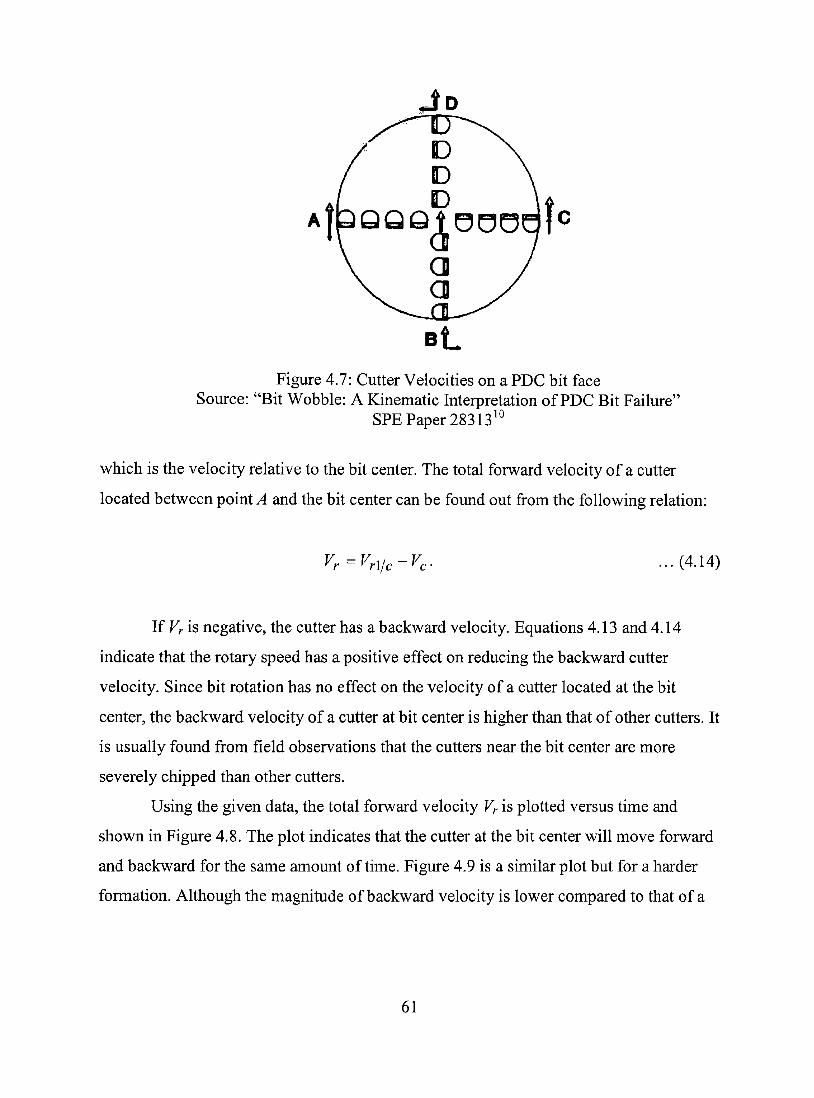
Figure 4.7: Cutter Velocities on a PDC bit face Source: "Bit Wobble: A Kinematic Interpretation of PDC Bit Failure"

SPEPaper 28313^^

which is the velocity relative to the bit center. The total forward velocity of a cutter

located between point A and the bit center can be found out from the following relation:

K=Vrl/c-~V,. ...(4.14)

If Vr is negative, the cutter has a backward velocity. Equations 4.13 and 4.14

indicate that the rotary speed has a positive effect on reducing the backward cutter

velocity. Since bit rotation has no effect on the velocity of a cutter located at the bit

center, the backward velocity of a cutter at bit center is higher than that of other cutters. It

is usually found from field observations that the cutters near the bit center are more

severely chipped than other cutters.

Using the given data, the total forward velocity Vr is plotted versus time and

shown in Figure 4.8. The plot indicates that the cutter at the bit center will move forward

and backward for the same amount of time. Figure 4.9 is a similar plot but for a harder

formation. Although the magnitude of backward velocity is lower compared to that of a

61

softer formation, the frequency of the vibration is increased in this case. Hence in hard

formation drilling, more cutter chipping is expected.

0.20

0.00 0.01 0.02 0.03 0.04 0.05 0.06 0.07 0.08 0.09 0.10

Time (sec)

Figure 4.8: Velocity of cutter at bit center (Er = 5x\0^psi)

0.15

0.00 0.01 0.02 0.03 0.04 0.05 0.06

Tíme (sec)

0.10

Figure 4.9: Velocity of cutter at bit center (Æ* = IxlO^ psi)

To minimize cutter failure of PDC bits, it is necessary to analyze the factors

affecting the backward velocities of the cutters. The pseudo-natural circular frequency is

given by:

62

0), (4.15)

If the stabiUzer position is high, then the value oíkd will be low and the pseudo-

natural frequency is dependent mainly on the formation rock property Er- It is also

observed that the drill-string vibration is sensitive to the lithology of the formation being

drilled. The effect of lateral contact area on backward cutter velocity at bit center is

shown in Figure 4.10. This plot indicates that the backward cutter velocity can be

effectively reduced by increasing the lateral contact area of the bit. This is in fact put into

practice in field by utiUzing a wider low friction pad.

0.80

OJO

0.60

J" 0.50

é o 0.40 > L.

^ 0.30

0.20

(Frequency Ratio = 0.5, Damping Factor = 0.5)

0.10

0.00 3 4 5 6 7

Lateral Conîact Area, in**2

8 9

Figure 4.10: Effect of Lateral Contact Area on Cutter Backward Velocity

The effect of weight of bit on backward cutter velocity is shown in Figure 4.11.

From the plot it is observed that a heavy bit is better than a lighter bit for controlling

backward cutter velocity. The effect of stabilizer position on backward cutter velocity is

63

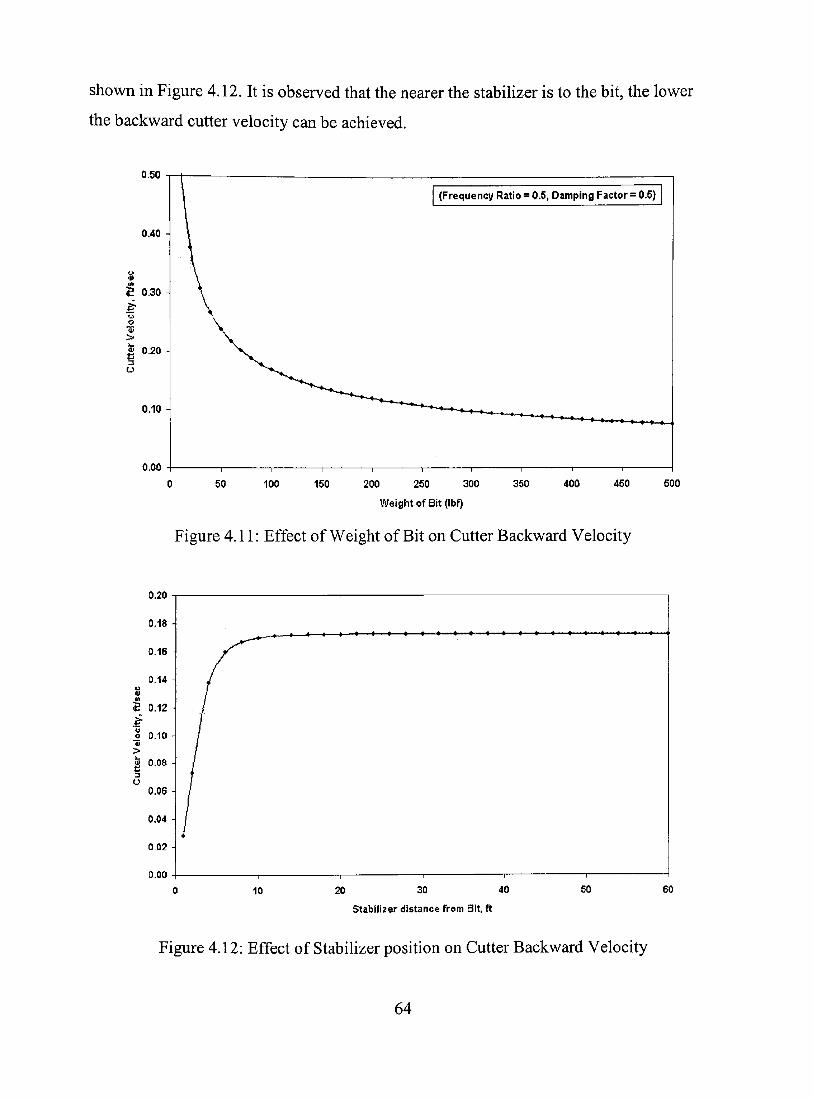
shown in Figure 4.12. It is observed that the nearer the stabilizer is to the bit, the lower

the backward cutter velocity can be achieved.

0.50

50 100 150 200 250 300 360 400 450 600

WeightofBit(lbf)

Figure 4.11: Effect of Weight of Bit on Cutter Backward Velocity

0.18 -

0.16

0.14 -u 01 tfl

Ê 0.12 ^ o 0.10 -4> > S 0.08 -

0.06 -

0.04 -

0.02 -

0.00 -

/

/

/

/

/

1 1 — — 1 1 1

10 20 30 40

Stabîllzer dîstance from Bit, ft

60 60

Figure 4.12: Effect of Stabilizer position on Cutter Backward Velocity

64

Figure 4.13 shows the effect of drill-collar stiffness on backward cutter velocity

indicating that increasing drilI-coUar stiffness reduces backward cutter velocity when the

stabilizer is placed close to the bit. The effect of viscous damping factor on backward

cutter velocity is shown in Figure 4.14. It indicates that viscous drilling fluids are helpful

in reducing the cutter backward velocity.

0,16

0.15 ^

0.14

0.13

Dhrahc-e of Stsbiliaer from Sit = 5 ft

Distance of Stabîliserfrom Bi t» 3 ft

Drill-Coliar Stlffnôss {x Ê+Ô7 ibf/in^)

Figure 4.13: Effect of DriII CoIIar Stifftiess on Cutter Backward Velocity

0.6 0.8

Damping Factor

1.6

Figure 4.14: Effect of Viscous Damping Factor on Cutter Backward Velocity

65

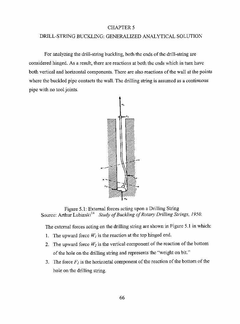
CHAPTER 5

DRILL-STRING BUCKLING: GENERALIZED ANALYTICAL SOLUTION

For analyzing the drill-string buckling, both the ends of the drill-string are

considered hinged. As a result, there are reactions at both the ends which in tum have

both vertical and horizontal components. There are also reactions of the wall at the points

where the buckled pipe contacts the wall. The drilling string is assumed as a continuous

pipe with no tool joints.

Figure 5.1: Extemal forces acting upon a Drilling String Source: Arthur Lubinski "^ Study ofBuckling ofRotary Drilling Strings, 1950.

The extemal forces acting on the drilling string are shown in Figure 5.1 in which:

1. The upward force Wi is the reaction at the top hinged end.

2. The upward force W2 is the vertical component of the reaction of the bottom

of the hole on the drilling string and represents the "weight on bit."

3. The force F2 is the horizontal component of the reaction of the bottom of the

hole on the drilling string.

66

4. The horizontal force F} is the reaction of the wall of the hole on the drilling

string if the pipe is buckled.

Two additional forces not shown in the above figure are the weight of the pipe

which is a vertical downward force, and the buoyancy which is a vertical upward force,

both appUed at the center of gravity of the drilling string. The influence of viscous forces

on the drill-string and the jet forces on the bit are neglected as they are small when

compared to the weight on the bit. When W^^Q, there is no weight on the bit and the

drilling string is straight resulting in an elastic equilibrium. If a lateral force is applied

and a small deflection is produced, this deflection disappears when the lateral force is

removed and the pipe becomes straight again. If W2 is increased, but maintained below a

certain critical value, the straight form remains stable. If the critical value of W2 is

reached, the straight form of the pipe becomes unstable; i.e., if a lateral force, however

small is appUed and a small deflection is produced, this deflection does not disappear

when the lateral force is removed. On the contrary, the deflection increases until a bent

form of stable equilibrium known as buckling is reached. The Xaxis is defined as the axis

of the hole and taken to be positive downwards. The point of origin is defined as the

neutral point. The 7axis is taken as positive to the right. The plane of theXand Faxes is

the plane of smallest flexural rigidity in which the buckling occurs. The units of X and Y

are in feet. The bending moment Mof the buckled string expressed in units oflbfft can

be given by:

d^Y M = E I ^ . . . (5.1)

dX^

where E is the Young's Modulus of elasticity of steel and/is the moment of inertia of the

cross section. The units oíE and /are Ibf/ft^ and//'^, respectively. The rate of change of

the bending moment is defined as the shear force and is obtained by differentiating

equation 5.1 with respect to X.

dh F,=EI^ . . . (5.2)

dX^

67

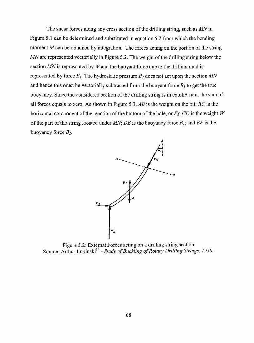
The shear forces along any cross section of the drilling string, such as MNin

Figure 5.1 can be determined and substituted in equation 5.2 from which the bending

moment M can be obtained by integration. The forces acting on the portion of the string

MN are represented vectorially in Figure 5.2. The weight of the drilling string below the

section MN is represented by W and the buoyant force due to the drilling mud is

represented by force B}. The hydrostatic pressure B2 does not act upon the section MN

and hence this must be vectorially subtracted from the buoyant force B} to get the tme

buoyancy. Since the considered section of the drilling string is in equilibrium, the sum of

all forces equals to zero. As shown in Figure 5.3, AB is the weight on the bit; BC is the

horizontal component of the reaction of the bottom of the hole, or Ff, CD is the weight W

of the part of the string located under MN\ DE is the buoyancy force Bj\ and EF is the

buoyancy force B2.

• ^ N

Figure 5.2: Extemal Forces acting on a drilling string section Source: Arthur Lubinski "^ - Study ofBuckling ofRotary Drilling Strings, 1950.

68

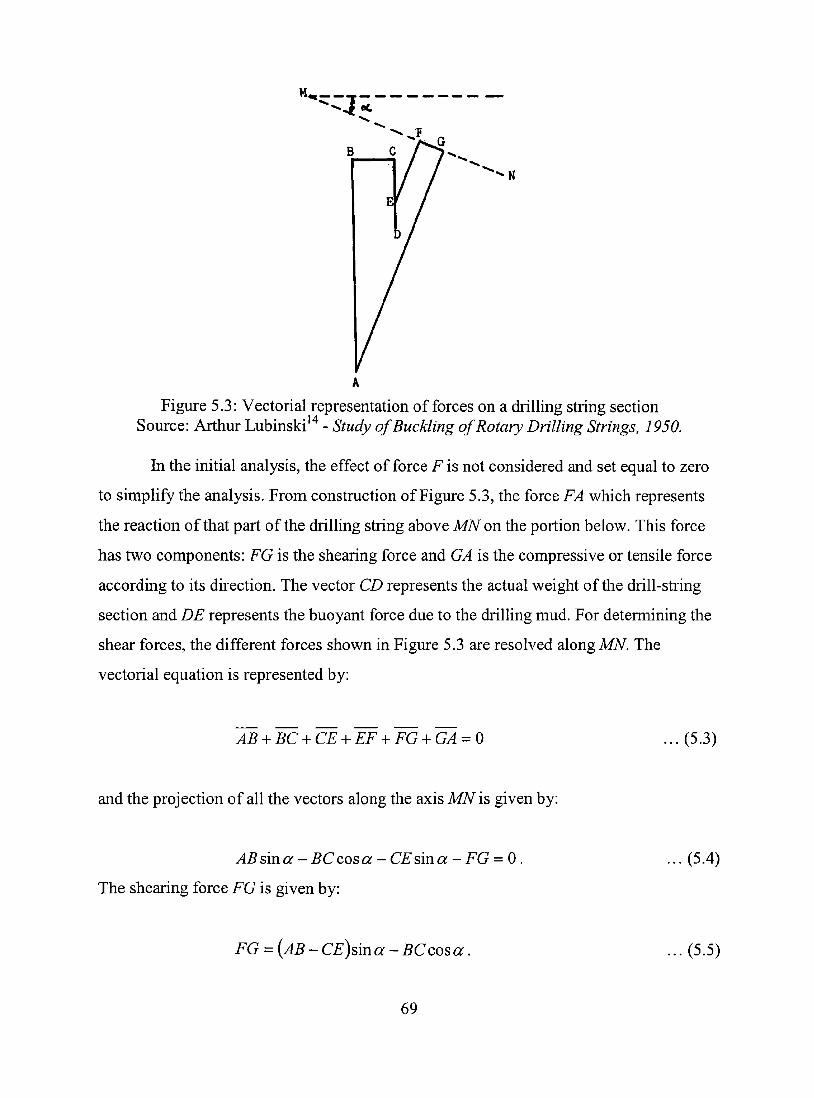
M. "J

B C

^ N

Figure 5.3: Vectorial representation of forces on a drilling string section Source: Arthur Lubinski "* - Study ofBuckling ofRotary Drilling Strings, 1950.

In the initial analysis, the effect of force F is not considered and set equal to zero

to simplify the analysis. From constmction of Figure 5.3, the force FA which represents

the reaction of that part of the drilling string above MN on the portion below. This force

has two components: FG is the shearing force and GA is the compressive or tensile force

according to its direction. The vector CD represents the actual weight of the drill-string

section and DE represents the buoyant force due to the drilling mud. For determining the

shear forces, the different forces shown in Figure 5.3 are resolved along MN. The

vectorial equation is represented by:

AB-\-BC-\-CE-\-EF-\-FG + GA = 0 . (5.3)

and the projection of all the vectors along the axis MN is given by:

ABsina- BCcosa-CEsina -FG = 0

The shearing force FG is given by:

(5.4)

FG = {AB - CE)sma-BCcosa . (5.5)

69

Under actual conditions in the hole, the angle a is very small. Therefore cos a=\ and sin

a = tan a. Then, equation 5.5 reduces to

FG = {AB-CE)\'âxia-BC (5.6)

The buoyancy factor is given by:

B.F = \ r \

Pmud

\Psteel j

...(5.7)

Letjo represent the weight of the drilling string in mud (units oîlbflft) which is equal to

the product of the actual weight of the drilling string in air and equation 5.7. LetXy and

X2 designate, respectively, the values of X for the two ends of the drilling string. Then:

X,=-W,

Xo =

P W2

(5.8)

Equation 5.5 can be re-written as follows:

F, = [W2-p{X2 -X)tana]-F2 (5.9)

Substituting in equation 5.9 the value 0ÍX2 from equation 5.8 and replacing tan a with

-dYldX, we get:

F, =-pX — -F2 ' dX ^

(5.10)

70


d^Y „dY EI—- + pX— + F2=0 ...(5.11)

dX^ dX

Equation 5.11 represents the differential equation of the buckled drilling string. Let

X = mx ...(5.12)

and Y = my ...(5.13)

where m is a constant which will be defined later.

We have from above two equations

dY _dy

dX dx

d^Y _ 1 d^y

dX^ m dx^

d^Y ^ 1 d^y

dX^ m^ dx^

Substituting equations 5.12, 5.14, and 5.16 into equation 5.11, we get

(5.14)

...(5.15)

(5.16)

d y p 3 dy F2 2 r\ c< \n\ — ^ + —m^x — + — m Ô ... (5.17) j;^3 EJ dx EI

71

The value of m is chosen such that

Let cbedefinedas:

3 EI m^ =— ...(5.18)

Fo c = -^ ...(5.19)

pm

Substituting equations 5.18 and 5.19 into equation 5.17, we get

^ + x ^ + c = 0 ...(5.20) dx^ dx

Substituting equations 5.15 and 5.18 into equation 5.1, we get

,2 M = pm^—f ...(5.21)

dx^

Equation 5.18 shows that m is expressed inft and equations 5.12, 5.13, 5.14, 5.19, and

5.21 show that;:,,)^, dyldx^ (^yldx ^ and c are dimensionless. Consequently, the analysis

made with these factors will be altogether general and independent of the drilling string

and drilling fluid.

The solution to the differential equation defmed by equation 5.21 and shown

below is required.

d y dy . — f + JC — + c = 0 dx^ dx

Let z = ^ ...(5.22) dx

72

Substituting equation 5.22 into the above differential equation, we get

dh_ dx

+ xz + c = 0 ...(5.23)

The solution to equation 5.23 can be expressed in terms of a power series defined by:

00

z= ^ a „ x " . «=0

...(5.24)


7Z-2 00

X«(«- l )o„x"-^ + ^fl„;c"-^^+c = 0. «=0 «=0

(5.25)

Equation 5.25 is a polynomial fimction in powers of x and satisfies for any value oíx. If

this is tme then the coefficients of x' , x\ x ^ x^, etc. must all be equal to zero.

Coefficient of x

Coefficient of .x

Coefficient of x

Coefficient of x

Coefficient of x'

Coefficient of x"

Coefficient of x'

2^2 + c = 0 => í32 -^2

aQ + 2.3^3 = 0 => «3 = -

ai +3.4^4 = 0 => «4 = -

«2 + 4.5(35 = 0 =^ «5 = -

ao_ 2.3

fL 3.4

^2 ^

4.5 2.4.5

^3 O ^3 + 5.6^5 = 0 => a^ = =

«4 + 6.7^7 = 0 => ay =

«5 +7.8^8 =0=> ag =•

5.6 2.3.5.6

^4 ãi

6.1 3.4.6.7

a^ c

7.8 2.4.5.7.8

73

Substituting the above coefficients into equation 5.25, we get

C 2 Ô 3 í l 4 C 5 « 0 fí ^] 7 C 8

z = ao+atX x^ ^x^ ^-x^ + x^ + ^ x ' ' + — x ' x° + 2 2.3 3.4 2.4.5 2.3.5.6 3.4.6.7 2.4.5.7.8

«0 1 - ^ + 2.3 2.3.5.6 2.3.5.6.8.9

+ ... + aix 1 + + 3.4 3.4.6.7 3.4.6.7.9.10

^x' 2

, x' x' 1 + 4.5 4.5.7.8 4.5.7.8.10.11 + ..(5.26)

z = ^ = aF(x)-\-bG(x) + cH(x) dx

...(5.27)

where F(x), G(x), and H(x) are the terms within brackets as defined in equation 5.26

Integrating equation 5.27, gives

y = aS(x) + bT(x)-\-cU(x)-\-g ..(5.28)

Differentiating equation 5.27 gives

d^

dx^ = aP(x) + bQ(x) + cR(x) (5.29)

The fiinctions in equafions 5.27, 5.28, and 5.29 are defined as foUows:

F{x) = \- — + "" + 2.3 2.3.5.6 2.3.5.6.8.9

(5.30)

G(x) = X , x' x' 1 + 3.4 3.4.6.7 3.4.6.7.9.10 + ... (5.31)

74

H(x) = - ~ 2

, x' x' 1 + 4.5 4.5.7.8 4.5.7.8.10.11 + ., (5.32)

S(x) = X

T(x) = X

, x' x' 1 + 2.3.4 2.3.5.6.7 2.3.5.6.8.9.10

1 x' x' +

+ ..,

2 3.4.5 3.4.6.7.8 3.4.6.7.9.10.11 +

..(5.33)

(5.34)

U(x) = - X 1 J

\ X X

+ X

3 4.5.6 4.5.7.8.9 4.5.7.8.10.11.12 + . (5.35)

P(x) = -, x' x' I +

3.5 3.5.6.8 3.5.6.8,9.11 ...(5.36)

3 6 Q(x) = \-^+ ^

3 3.4.6 3.4.6.7.9 + ... (5.37)

R(x) = -X 3 6

X X

1 + X

2.4 2.4.5.7 2.4.5.7.8.10 + (5.38)

The fiinction values for equations from 5.31 through 5.38 have been calculated by

writing computer program using MATLAB. The computer source code is enclosed in B-1

of Appendix B. The curves generated for above fianctions are plotted in dimensionless

units and are shown in Figures 5.4, 5.5, and 5.6, respectively. These curves can be used

as reference for calculating the deflections once the equation coefficients are determined.

75

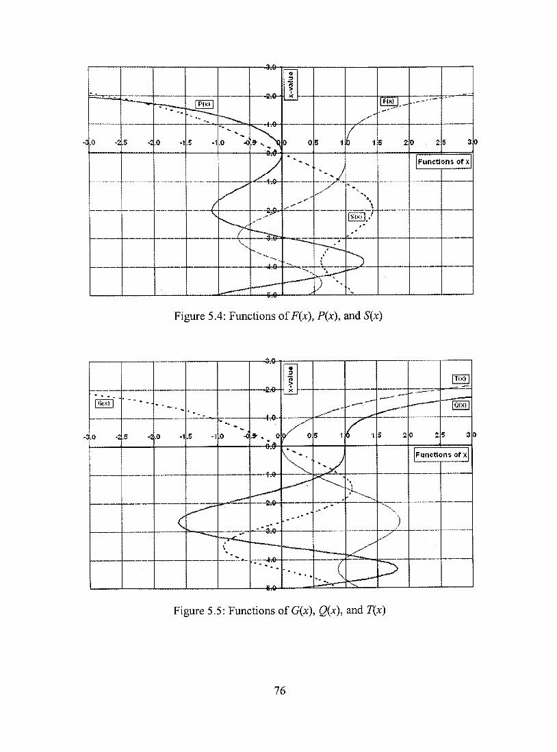
-M

Figure 5.4: Functions of F(x), P(x), and S(x)

Figure 5.5: Functions of G(x), Q(x), and T(x)

76

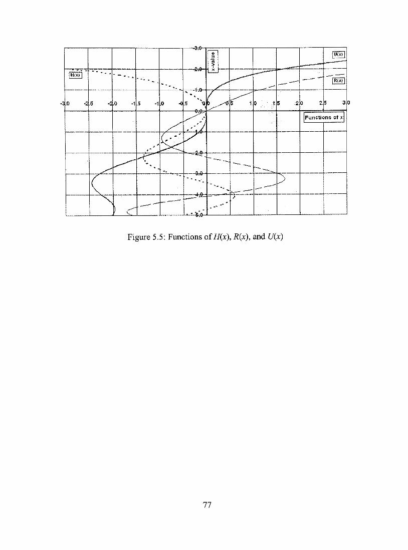
Figure 5.5: Functions ofH(x), R(x), and U(x)

77

CHAPTER 6

DRILL-STRING BUCKLING - ANALYSIS AND DISCUSSION

6.1 Critical Buckling Condition of the First Order

Let X} and x^ designate the values of x for the upper and lower ends of the drilling

string respectively. The distance X} represents the distance between the neutral point and

the top of the hole. The distance x^ represents the distance between the bit and neutral

point. Let P}, Q}, R}, Sj etc. denote the values of P(jc), Q(x), R(x), S(x), etc, at x=X} and

Pi Qi Ri S2, etc, denote the values of P(x), Q(x), R(x), S(x), etc, at x=X2. As both the

ends of the drilling string are hinged, the bending moments at these two ends are equal to

zero. From equations 5.21 and 5.29, we get

aPi+bQi-\-cRi =0 ...(6.1)

aP2-\-bQ2-\-cR2 =0. (6.2)

At both the ends, y=0 and equation 5.28 gives for both the ends:

aSi-\-bTi-\-cUi-\-g = 0 . (6.3)

aS2-^bT2-\-cU2-\-g = 0 ..(6.4)

Eliminating g from equations 5.41 and 5.42, we get

a{Si-S2)^b{T^-T2) + c{U^-U2)=0 ...(6.5)

Equations 6.1, 6.2, and 6.5 together yield the relationship between X} and x^ for buckling

to occur. This is obtained by eliminating the coefficients and equating the determinant to

zero.

î ôi î

Pl Ql ^2 {8,-82) {TI-T2) {UI-U2)

(6.6)

78

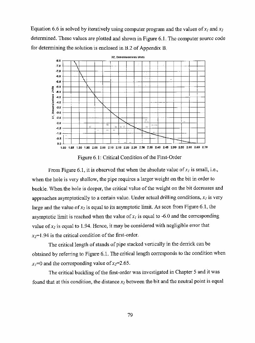
Equation 6.6 is solved by iteratively using computer program and the values of x/ and X2

determined. These values are plotted and shown in Figure 6.1. The computer source code

for determining the solution is enclosed in B.2 of Appendix B.

X2, Dlmensionless Units -S.O

-7.5

-7.0

-G.5

•e.o

-6.5

-6.0

-4.5

-4.0

-3.5

-3.0

-2.5

-2.0

-1.6

-1.0

-0.5

0.0

\ \

\ \ ,

s N. \ ,

^

^

> \

sl \ N

- ^

~. ~

„

1.80 1,85 1.90 1S5 2.00 2.05 2.10 2.15 2.20 2.25 2.30 2.35 2.40 2.45 2.50 2.55 2.60 2.65 2.70

Figure 6.1: Critical Condition of the First-Order

From Figure 6.1, it is observed that when the absolute value of x; is small, i.e.,

when the hole is very shallow, the pipe requires a larger weight on the bit in order to

buckle. When the hole is deeper, the critical value of the weight on the bit decreases and

approaches asymptotically to a certain value. Under actual drilling conditions, xy is very

large and the value of x^ is equal to its asymptotic limit. As seen from Figure 6.1, the

asymptotic limit is reached when the value of x; is equal to -6.0 and the corresponding

value of X2 is equal to 1.94. Hence, it may be considered with negligible error that

X2=1.94 is the critical condition of the first-order.

The critical length of stands of pipe stacked vertically in the derrick can be

obtained by referring to Figure 6.1. The critical length corresponds to the condition when

x/=0 and the corresponding value of X2=2.65.

The critical buckling of the first-order was investigated in Chapter 5 and it was

found that at this condition, the distance x between the bit and the neutral point is equal

79

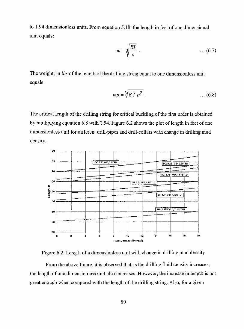
to 1.94 dimensionless units. From equation 5.18, the length in feet of one dimensional

unit equals:

m = 3, EI

.,.(6.7)

The weight, in Ibs of the length of the drilling string equal to one dimensionless unit

equals:

mp = ^ÊIp (6.8)

The critical length of the driUing string for critical buckling of the first order is obtained

by multiplying equation 6.8 with 1.94. Figure 6.2 shows the plot of length in feet of one

dimensionless unit for different drill-pipes and drill-collars with change in drilling mud

density.

8 10 12

Flujd Dens ty (Ibm/gai)

20

Figure 6.2: Length of a dimensionless unit with change in driUing mud density

From the above figure, it is observed that as the drilling fluid density increases,

the length of one dimensionless unit also increases. However, the increase in length is not

great enough when compared with the length of the drilling string, AIso, for a given

80

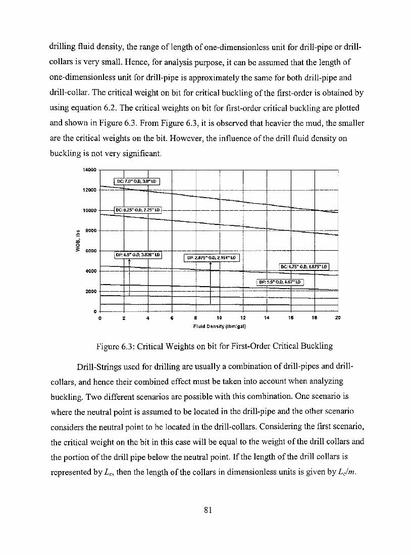
drilling fluid density, the range of length of one-dimensionless unit for drill-pipe or drill-

collars is very small. Hence, for analysis purpose, it can be assumed that the length of

one-dimensionless unit for drill-pipe is approximately the same for both drill-pipe and

drill-coUar. The critical weight on bit for critical buckling of the first-order is obtained by

using equation 6.2. The critical weights on bit for first-order critical buckling are plotted

and shown in Figure 6.3. From Figure 6.3, it is observed that heavier the mud, the smaller

are the critical weights on the bit. However, the influence of the drill fluid density on

buckling is not very significant.

14000

12000

10000

o ^ 6000

4000

2000

1 DC;7.0"O4),3.0"l.D |

1 DC: 6.25** OS), 2^5" W —

|DP:4^"bj).3.826"I.D 1 1

DP; 2.875" OJ), 2.151" 1.0

. ,

=•=*- . „

-^.«=^

1 DC 4.75" OJ), 1^75" LO |

— ^ 1 DP: 5.5" 0,D, 4,67" U) |

.-.-

' • ' " " '

8 10 12

riuld Density {ibm/^3\)

14 16 18 20

Figure 6,3: Critical Weights on bit for First-Order Critical Buckling

Drill-Strings used for drilling are usually a combination of drill-pipes and driU-

coUars, and hence their combined effect must be taken into account when analyzing

buckling. Two different scenarios are possible with this combination. One scenario is

where the neutral point is assumed to be located in the drill-pipe and the other scenario

considers the neutral point to be located in the drill-collars. Considering the first scenario,

the critical weight on the bit in this case will be equal to the weight of the drill collars and

the portion of the drill pipe below the neutral point. If the length of the driU coUars is

represented by Zc, then the length of the collars in dimensionless units is given by LJm.

81

For critical conditions of the first-order, the length in dimensionless units of the portion

of the driU-pipe below the neutral point is given by:

\.94-Ljm. ...(6.9)

The weights of these two portions in the presence of drilling fluid are LcPc and

(l .94 - L^ /m)m Pp, respectively. The sum of the weights equal to the weight W} and

equals:

Wi=L,(p,-pp)+\.94mpp. ...(6.10)

From equation 6.10, it is observed that the critical weights are linear fiinctions of

the total length of the drill-collars. The slope of the straight line and the>'-intercept being

equal to Pc-Pp and \.94mpp, respectively. This is represented by the inclined line in

Figure 6.4. For the second scenario, the whole weight on the bit is given by the drill

collars. The critical values of the weight on bit cannot be increased by adding more drill

coUars. The second scenario corresponds to the horizontal Une of Figure 6.4. The dotted

lines in Figure 6.4 represent similar conditions in the presence of higher drilling fluid

density. From Figure 6.4 to prevent first-order buckling in the presence of 10 Ibm/gal

drilling fluid, the weight on the bit should not exceed 8600 Ibs. In the presence of 16

Ibm/gal drilling fluid, the weight on bit should not exceed 7800 Ibs. If the weight on bit

exceeds these values, then the drill string will buckle once until the weight on bit exceeds

16600 and 15400 Ibs, respectively, when the drill string will buckle a second time. The

critical weight on the bit can be increased by using drill-collars with bigger size, high

stifftiess and elasticity values.

Figure 6.5 shows the effect of driU coUar size on first order buckling with a radial

clearance of 2.75-in. between the hole and the drill collar and in the presence of 12.0

Ibm/gal drilling mud. The drill collar inside diameter is taken as 1.875-in. It is observed

that the critical weight on the bit increases as the drill collar size increases. This is due to

the increase in stifftiess of the drill collars with increasing size. Similar plots are shown in

Figures 6.6 and 6.7 for drill collar inside diameters of 2.5-in and 3.0-in, respectively. As

82

the driU collar inside diameter increases, the critical weight on bit also increases and

similar profiles as in Figure 6.5 are observed.

Dríll-Pípe: 4,5-in, 16.6 Ib/ft. Drîll-Collar: 6.25-ln O.D,2.25-in LD.SÛ.S Ib/ft 18000

16000

14000

12000

c o

£ 8000

6000

4000

2000

lOlbm/galMud

/

/ ' / /

/ /

/ /

16lbm/galMud

Drjlllng Stríng Buckled Once

// lOlbm/galMud

/'/

/ ' / •

/ / ' //'

1 1 1 1 '—\

16lbm/galMud

Straight Drílling String

6 8 10 12

Number of Dríll Coflars

14 16 18 20

Figure 6.4: Buckling Conditions for Combination Drilling Strings

16000

14000

12000

£k

i • x: o

10000

8000

6000

4000 —

2000

! 1 m»\ Denslty: 12.0 Ibm/gal

Oearance: 2.7S-in. Dr^CoÍtar 1.0:1.875-111.

• í

• y

* y ^

120

105

90 X t o

- 7 5

15» «í

60 w gî

30 « 'C

o 15

3.0 3.5 4.0 4.5 5.0 5.5 6.0 6.5 7.0 7.5 8.0

OrillCoIlarO.D, in.

Figure 6.5: Influence of DrilI-CoIIar size on Buckling (I.D=1.875-z^)

83

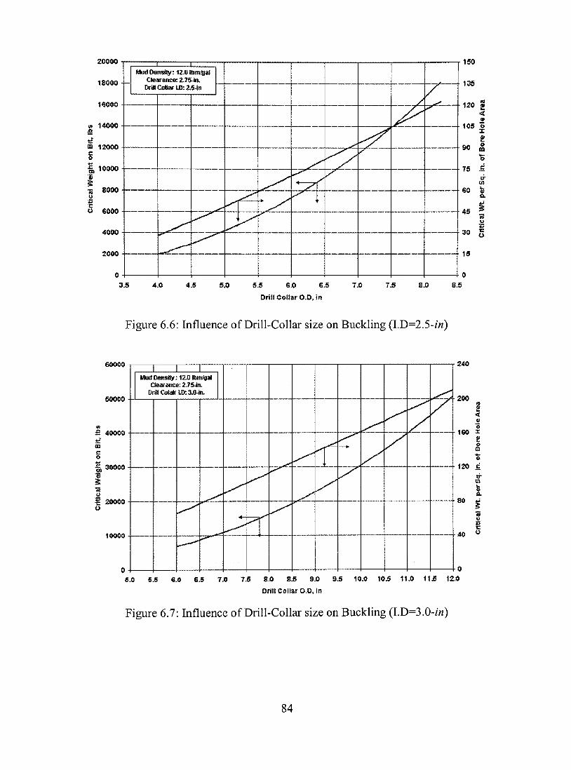
20000

180<K)

16000

m 14000

m 120CK) c o U. lOOW

S 6000

4<m

2ÔÔ0 —

--_

1 1 Mud Dens^ : 12.0 mmS^l

Clearmtce: 2.7S~Ín. Dr»Co^rLD:2.S-in

._

—

—

' ' ..^"""'''''^

-py^—

E

^Z ^^

150

136

120

105

90

76

60

45

30

16

3.6 4.0 4.5 5.0 5.5 6.0 6.5

Drill Coilar O.D, in

7.0 7.5 8,0 8.5

Figure 6.6: Influence of DriII-CoIIar size on Buckling (l.D=2.5~in)

60000

5(K)00

£ 4<K)00

c: o

1 3«)00

20000

10000

1 1 1 Mud û e n ^ : 12.0 Ibm/gal

Cfe^ætGe: 2.7S'ín. Dri»Orfafrl.D:3.0.in.

-

~~—

.

—j L.„_ ~ - •

240

200 n

i < o

160 X o m o

120 c

80

40

5.0 53 6.0 6.5 7J0 7.5 S.O B3 9.0 B3 10.0 10.5 11J) 11.5 12.0

DriHCoHarO.D, in

Figure 6.7: Influence of DrilI-CoIIar size on Buckling (LD=3.0-z>2)

84

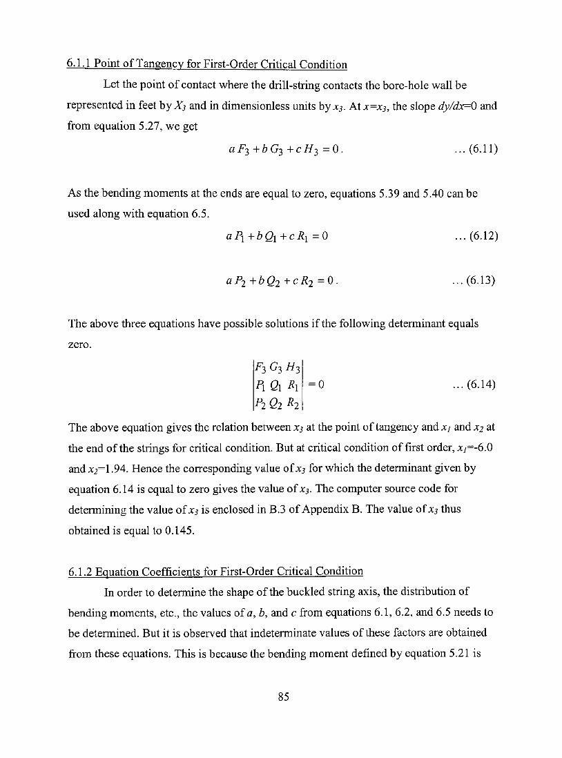
6.1.1 Point of Tangencv for First-Order Critical Condition

Let the point of contact where the drill-string contacts the bore-hole wall be

represented in feet by JSG and in dimensionless units by x . Atx=X3, the slope dy/dx=0 and

from equation 5.27, we get

aF^-\-bG2-\-cH^ =0. ...(6.11)

As the bending moments at the ends are equal to zero, equations 5.39 and 5.40 can be

used along with equation 6.5.

aPi-\-bQi-\-cRi =0 ... (6.12)

aP2+bQ2+cR2 = 0 . ...(6.13)

The above three equations have possible solutions if the following determinant equals

zero.

0 ...(6.14)

The above equation gives the relation between x^ at the point of tangency and X} and x^ at

the end of the strings for critical condition. But at critical condition of first order, X}=-6.0

and X2=\ .94. Hence the corresponding value of xj for which the determinant given by

equation 6.14 is equal to zero gives the value ofxs. The computer source code for

determining the value oîxs is enclosed in B.3 of Appendix B. The value ofxs thus

obtained is equal to 0.145.

6.1.2 Equation Coefficients for First-Order Critical Condition

In order to determine the shape of the buckled string axis, the distribution of

bending moments, etc, the values of a, b, and c from equations 6.1, 6.2, and 6.5 needs to

be determined. But it is observed that indeterminate values of these factors are obtained

from these equations. This is because the bending moment defined by equation 5.21 is

85

F3

^l

Pl

G3

Qi

Qi

H3

Rx

Ri

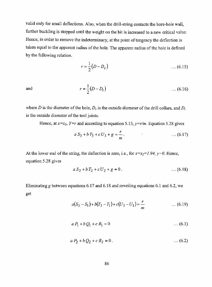
vaUd only for smaU deflections. AIso, when the drill-string contacts the bore-hole wall,

further buckling is stopped until the weight on the bit is increased to a new critical value,

Hence, in order to remove the indeterminacy, at the point of tangency the deflection is

taken equal to the apparent radius of the hole. The apparent radius of the hole is defined

by the following relation.

r = ^{D-D,) ...(6.15)

and r = ^{D-D,) ...(6.16)

where D is the diameter of the hole, D^ is the outside diameter of the driU collars, and A

is the outside diameter of the tool joints.

Hence, aXx=X3, Y=r and according to equation 5.13, j^=r/m. Equation 5.28 gives

û 5 3 + 6 r 3 + c t / 3 + g = —. - ...(6,17) m

At the lower end of the string, the deflection is zero, i.e., forx=X2=1.94, y=0. Hence,

equation 5.28 gives

aS2-\-bT2-\-cU2-^g = 0. ...(6.18)

Eliminating g between equations 6.17 and 6.18 and rewriting equations 6.1 and 6.2, we

get

^(^3 -Si)^b{T^ -Ti)+c{U^ -Ui) = - ... (6.19)

aPi-\-bQi-\-cRi =0 ...(6.1)

aP2-\-bQ2-\-cR2 = 0 . ... (6.2)

86

Substitutmgxy=-6.0, X2=\.94, andxi=0.145 in the above equations, the values oía(m/r),

b(m/r), and c(m/r) can be calculated. From equations 6.1 and 6.2, we get

a ^ _ ^

QxRi -QiRi ~ R\P2 -RiP\ ~ PiQi -PiQi

a = 9l^lzQAc . . .(6.20) P\Q2-P2Q\

^^R^PIZMLC. ...(6.21) ^102-^201

Substituting equations 6.14 and 6.15 into equation 6.13 gives:

c = —X î . ...(6.22) m (5 _s^)Q^^2-Q2R\ ^(y _T^f\P2 -R2P\ ^ ( ^ _ ^ )

^PlÔ2-^2Ôl ^ P l Ô 2 - ^ 2 a

6.2 Critical Buckling Conditions above First-Order

After the drill string undergoes first-order buckling and if the weight on the bit

goes on increasing, there is a tendency for the drill string to buckle a second time. In such

a situation, the differential equation defined by equation 5.11 does not hold true for the

whole length of the drilling string. For the upper portion of the drilling string (located

above the point of tangency), the force F which is the reaction of the wall of the hole

against the pipe needs to be considered. Hence, equation 5.11 is modified as:

d^Y dY E I ^ + pX — + F2-F = 0. ...(6.23)

dX^ dX ^

The equations 5.19 and 5.23 are also modified as follows:

c = ^^/^ ...(6.24) pm

87

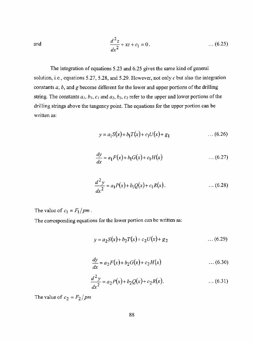
d'^z and — ^ j c z + ci =0. ...(6.25)

Jx^

The integration of equations 5.23 and 6.25 gives the same kind of general

solution, i.e., equations 5.27, 5.28, and 5.29. However, not only c but also the integration

constants a, b, and g become different for the lower and upper portions of the drilling

string. The constants ûy, 67, c/ and a^, b^, c^ refer to the upper and lower portions of the

drilling strings above the tangency point. The equations for the upper portion can be

written as:

y = aiS{x)-\-biT{x)-\-ciU{x)-\-gl ... (6.26)

^ = aiF(x) + 6iG(x)+ci//(x) ... (6.27) dx

^ = aiP{x) + biQ{x) + ciR{x). ... (6.28) dx^

The value of cj = F^ /pm .

The corresponding equations for the lower portion can be written as:

y = a28{x)+b2T{x) + C2U{x)+g2 . . . (6.29)

^ = a2F{x)+b2G{x)+C2H{x) ... (6.30) dx

2

2 Í ^ = a2P{x)-^b2Q{x) + C2R{x). . . . (6.31) dx

The value of c^ = F^ /pm

88

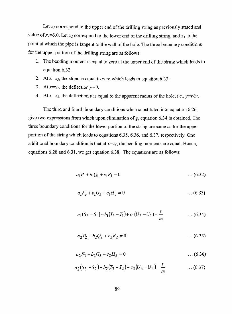
Let X} correspond to the upper end of the drilling string as previously stated and

value of xy=6.0. Let x^ correspond to the lower end of the drilling string, and X3 to the

point at which the pipe is tangent to the wall of the hole. The three boundary conditions

for the upper portion of the drilling string are as follows:

1. The bending moment is equal to zero at the upper end of the string which leads to

equation 6.32.

2. At x=X3, the slope is equal to zero which leads to equation 6.33.

3. Atx=xy, the deflectionj;=0.

4. At x=X3, the deflection j ; is equal to the apparent radius of the hole, i.e., y=r/m.

The third and fourth boundary conditions when substituted into equation 6.26,

give two expressions from which upon elimination of g, equation 6.34 is obtained. The

three boundary conditions for the lower portion of the string are same as for the upper

portion of the string which leads to equations 6.35, 6.36, and 6.37, respectively. One

additional boundary condition is that at x=jC5, the bending moments are equal. Hence,

equations 6.28 and 6.31, we get equation 6.38. The equations are as follows:

aiPi + biQx + cii?i = 0 ... (6.32)

^1^3 + 61G3 + C1//3 = 0 ... (6.33)

« l f e - ^ l ) + ^ l ( ^ 3 - ^ l ) + q ( ^ 3 - t ^ l ) = - .. .(6.34)

« 2 ^ 2 + ^ 2 0 2 + ^ 2 ^ 2 = 0 ...(6.35)

«2^3 -^b^Gi^ +C2//3 = 0 ... (6,36)

a2{S^-S2)^b2{T^-T2) + C2{U^-U2)-- . . .(6.37)

89

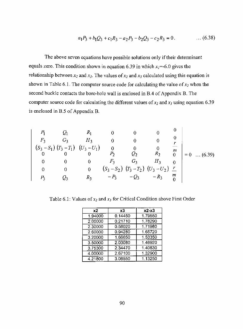
«1^3 +^103 + q ^ 3 -«2^3 ~hQ2> -^2^3 =0 ...(6.38)

The above seven equations have possible solutions only if their determinant

equals zero. This condition shown in equation 6.39 in which xy=-6.0 gives the

relationship between x^ and X3. The values of x and X3 calculated using this equation is

shown in Table 6.1. The computer source code for calculating the value of Xi when the

second buckle contacts the bore-hole wall is enclosed in B.4 of Appendix B. The

computer source code for calculating the different values of x^ and X3 using equation 6.39

is enclosed in B.5 of Appendix B.

î Q\ Ri

F^ C^ H^

{8^-8,){T,-T,) ( f /3- í / i )

0

0

0

^ 3

0 0

0

3

0 0

0

Ô3

0

0

0

P2

P3

0

0

0 Ô2

G3

0

0

0

R2

H3

0

0 r

m 0

0 {82-82) {T3-T2) {U3-U2) L

-P3 -Q3 -R3 'H

0 ...(6.39)

Table 6.1: Values of x andxj for Critical Condition above First Order

x2 1.94000

2.00000

2.30000

2.60000

3.20000

3.50000

3.75300

4.00000

4.21800

x3 0.14450

0.21710

0.58020

0.94280

1.66650

2.03080

2.34470

2.67100

3.08550

x2-x3

1.79550

1.78290

1.71980

1.65720

1.53350

1.46920

1.40830

1.32900

1.13250

90

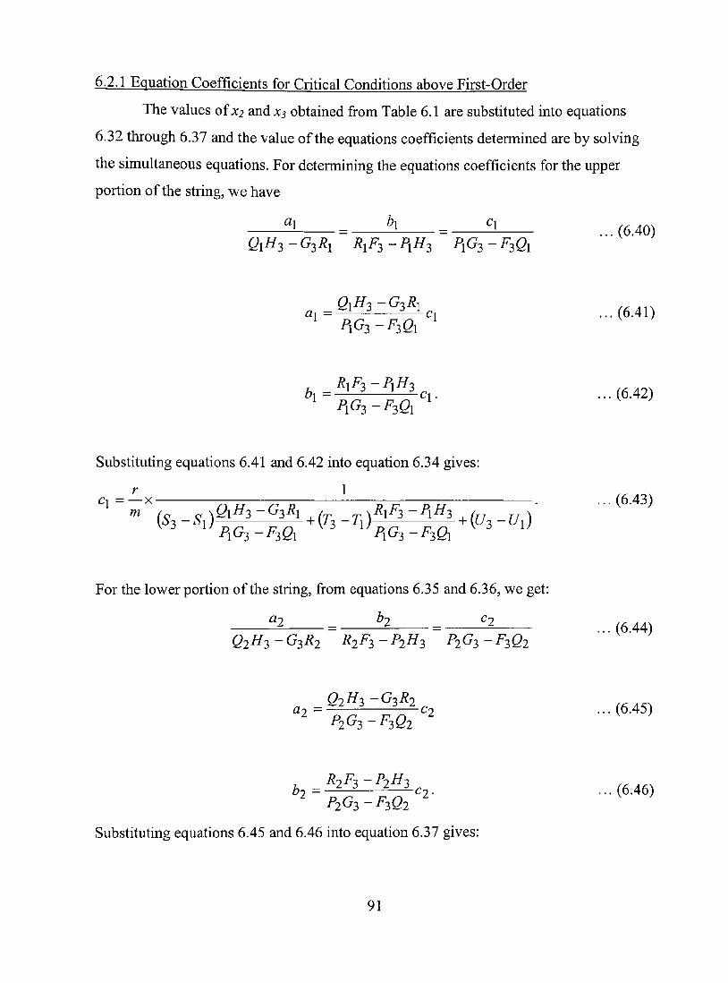
6.2.1 Equation Coefficients for Crítical Conditions above Fírst-Order

The values of x^ andxj obtained from Table 6.1 are substituted into equations

6.32 through 6.37 and the value of the equations coefficients determined are by solving

the simultaneous equations. For determining the equations coefficients for the upper

portion of the string, we have

«1 bi ci

QlH^ - G3R1 i?iF3 - P1//3 P1G3 - F^Qi

For the lower portion of the string, from equations 6.35 and 6.36, we get:

^2 = ^2 = ^^ Q2H2 - G2R2 R2P3 - P2H3 P2G3 - F3Q2


91

. (6.40)

Q,H,-G,R,

P1G2-F2Q1

RlFj-P^H^ ,^ .r.. b\ = -——zrTrî • • • • (6-42)

P1G3 - F^Qx


ci=—X . ...(6.43) m ^ _^^QiH3z^^(T _T)MlzMl + {u^_U,)

" P.G^-F^Q, 'P\G3-F3Qx

(6.44)

Q2H3-G2R2 ..... flT = Cj . . . ( 6 . 4 5 )

^2^3-^302

^ MIZM^C^. . . .(6.46) ^2^3-^302

6.3 Shape of the Buckled DrílUng String

Let the deflection coefficient h be defined by the following equation:

h = y — . ...(6.48) r

From equations 6.48 and 5.13, we get

Y = hr. ...(6.49)

From above equations, h is equal to unity for the deflection Y equal to the apparent radius

of the hole r. At the upper end of the string above the tangency point the deflection is

zero and equation 6.26 gives

0 = aiSi + bxTi + cit/i + g i . ... (6.50)

EUminatinggy between equations 6.26 and 6.50, we get:

y = a^{S-8^)+b^{T-T^)+c^{U-U^). ...(6.51)

At the lower end of the stríng, the deflection is equal to zero and equation 6.29 gives:

0 = fl2'^2+^2^2+C2t^2+^2^ ...(6.52)

Eliminating g2 between equations 6.23 and 6.52 gives:

y = a2{8-82)+b2{T-T2)+C2{U-U2). . . . (6.53)

92

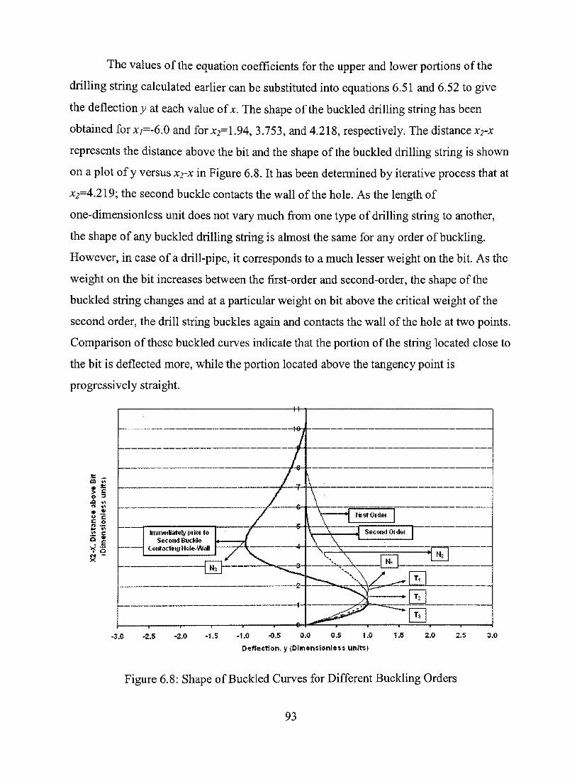
The values of the equation coefficients for the upper and lower portions of the

drilling string calculated eariier can be substituted into equations 6.51 and 6.52 to give

the deflectionj/ at each value of x. The shape of the buckled drilling string has been

obtained forxy=-6.0 and forx2=1.94, 3.753, and 4.218, respectively. The distancex2-x

represents the distance above the bit and the shape of the buckled drilling string is shown

on a plot of y versus x -x in Figure 6.8. It has been determined by iterative process that at

X2=4.219; the second buckle contacts the wall of the hole. As the length of

one-dimensionless unit does not vary much from one type of driUing string to another,

the shape of any buckled drilling string is almost the same for any order of buckling.

However, in case of a drill-pipe, it corresponds to a much lesser weight on the bit. As the

weight on the bit increases between the first-order and second-order, the shape of the

buckled string changes and at a particular weight on bit above the critical weight of the

second order, the drill string buckles again and contacts the wall of the hole at two points.

Comparison of these buckled curves indicate that the portion of the stríng located close to

the bit is deflected more, while the portion located above the tangency point is

progressively straight.

+1-

* * *> c

X

-3.0 •1.0 -03 0.0 0.5 1.0

D^flectjon. y (Dimensionldss unjt$)

Figure 6.8: Shape of Buckled Curves for Different Buckling Orders

93

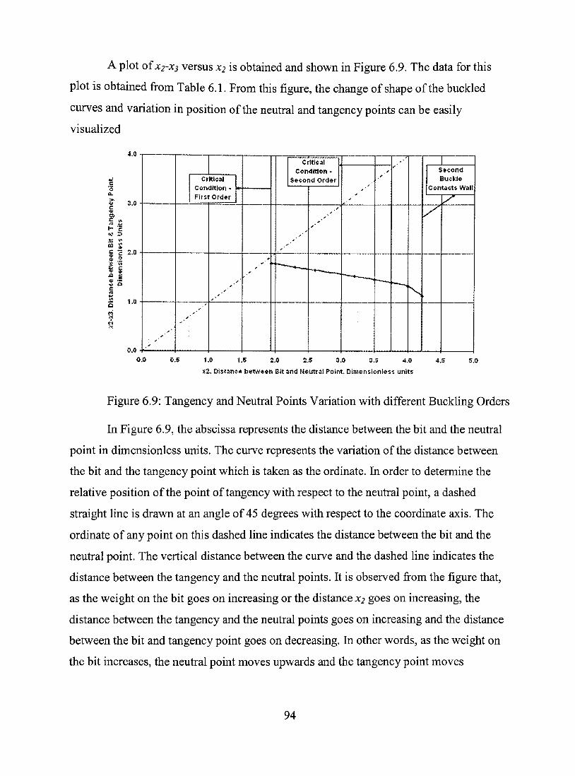
A plot of X2-Xi versus x is obtained and shown in Figure 6.9. The data for this

plot is obtained from Table 6.1. From this figure, the change of shape of the buckled

curves and varíation in position of the neutral and tangency points can be easily

visualized

c 41

4.0

3.0

f I 2.0 * .2

1.0

0.0

y j i

* .-'

Critlcal

Condition -First Ord*r

^' •'

4»

•

r

t'

/ /

^ •* f

f

Crítical Condítion -

Second Order

,-''

y

'

>'

i>

> ^ • ' "

1 Second Buckle

Contâcts Wall

0.0 0.5 1.0 1.5 2.0 2.5 3.0 3.5 4.0

x íí, Distanûe betwéftn Bit and Neutral Point. Dímensioniess units

4.5 5,0

Figure 6.9: Tangency and Neutral Points Variation with different Buckling Orders

In Figure 6.9, the abscissa represents the distance between the bit and the neutral

point in dimensionless units. The curve represents the varíation of the distance between

the bit and the tangency point which is taken as the ordinate. In order to determine the

relative position of the point of tangency with respect to the neutral point, a dashed

straight line is drawn at an angle of 45 degrees with respect to the coordinate axis. The

ordinate of any point on this dashed line indicates the distance between the bit and the

neutral point. The vertical distance between the curve and the dashed line indicates the

distance between the tangency and the neutral points. It is observed from the figure that,

as the weight on the bit goes on increasing or the distance x^ goes on increasing, the

distance between the tangency and the neutral points goes on increasing and the distance

between the bit and tangency point goes on decreasing. In other words, as the weight on

the bit increases, the neutral point moves upwards and the tangency point moves

94

downwards. The downward displacement of the tangency point becomes much faster

when the weight on the bit is increased between the critical value of the second-order and

the weight for which the second buckle contacts the wall of the hole.

It is also observed that at higher buckling orders the highest buckle contacts the

wall of the hole at the neutral point; and that, as the weight on the bit is increased, the

point of tangency is slightly displaced downward while the neutral point moves rapidly

upward. Knowledge of the location of the tangency point may be usefiil when drilling

hard formation below a soft and caving shale. If less weight than the critical weight of the

first-order is used while drilling in the caving shale in order to avoid caving and once the

hard formation is encountered, then the weight on the bit should not be increased

immediately. If the weight on the bit is increased immediately, the drilling string will

contact the caving shale wall above and caving could occur. One-and-half-dimensional

units should be drilled before weight on bit is increased and at that time, the weight on bit

should be increased immediately rather than progressively in order to obtain a tangency

point in the hard formation. It is observed that, drilling should be carried with a weight on

the bit corresponding to approximately 3.75 dimensionless units between the bit and the

neutral point but should not exceed 4.22 dimensionless units in order to keep the second

buckle from contacting the caving shale above. Higher values of weight on bit should not

be used before 4.2 dimensionless units of the hard formation are drilled.

The crítical weight for buckling of the second-order to occur is obtained by

multiplying equation 6.8 by 3.753 units. Figure 6.10 shows the crítical weight on bit for

second order buckling for different dríll pipes and drill collars. The magnitude of the

critical weights is higher than the corresponding weights of the first order buckling. As

the drílling fluid density increases, the crítical weight on bits decreases. However, the

decrease is very small when compared with the change in the drílling fluid density. The

computer source code for calculating the deflections of the buckled drílling stríng at each

position is enclosed in B.6 of Appendix B.

95

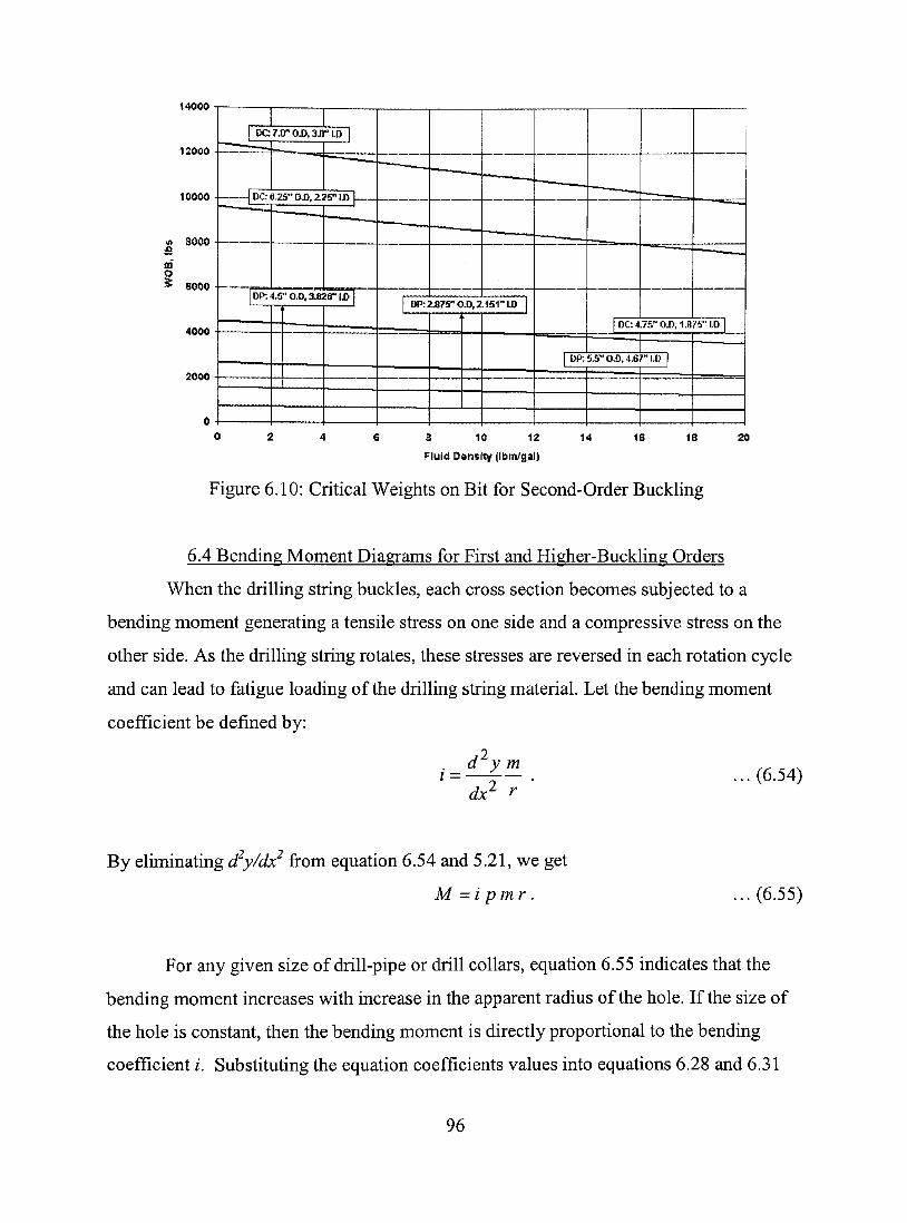
14000

2000

Figure 6.10: Crítical Weights on Bit for Second-Order Buckling

6.4 Bending Moment Diagrams for First and Higher-Buckling Orders

When the drilling stríng buckles, each cross section becomes subjected to a

bending moment generating a tensile stress on one side and a compressive stress on the

other side. As the drilling stríng rotates, these stresses are reversed in each rotation cycle

and can lead to fatigue loading of the drílling stríng materíal. Let the bending moment

coefficient be defined by:

i =

2 d y m

dx^ r ...(6.54)

By eliminating Sy/do^ from equation 6.54 and 5.21, we get

M =i pmr. ...(6.55)

For any given size of dríll-pipe or dríU collars, equation 6.55 indicates that the

bending moment increases with increase in the apparent radius of the hole. If the size of

the hole is constant, then the bending moment is directiy proportional to the bending

coefficient /. Substituting the equation coefficients values into equations 6.28 and 6.31

96

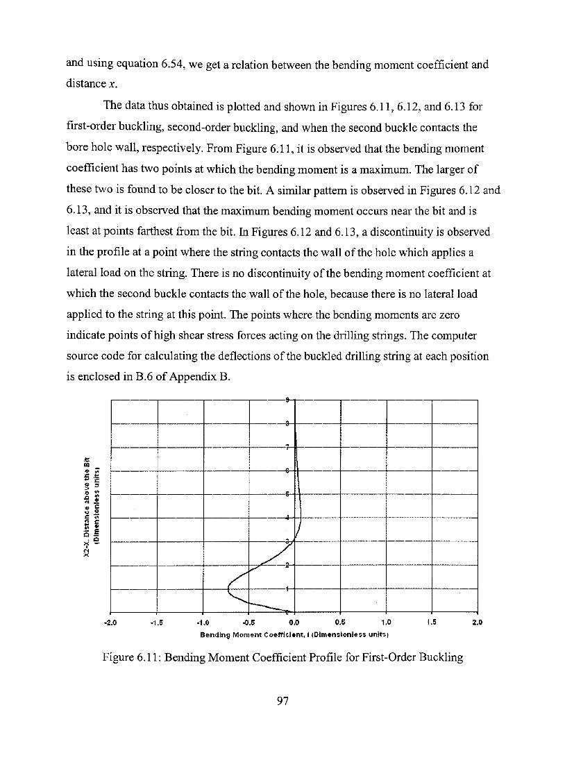
and using equation 6.54, we get a relation between the bending moment coefficient and

distance x.

The data thus obtained is plotted and shown in Figures 6.11, 6.12, and 6.13 for

first-order buckling, second-order buckling, and when the second buckle contacts the

bore hole wall, respectively. From Figure 6.11, it is observed that the bending moment

coefficient has two points at which the bending moment is a maximum. The larger of

these two is found to be closer to the bit. A similar pattem is observed in Figures 6.12 and

6.13, and it is observed that the maximum bending moment occurs near the bit and is

least at points farthest from the bit. In Figures 6.12 and 6.13, a discontinuity is observed

in the profile at a point where the stríng contacts the wall of the hole which appUes a

lateral load on the stríng. There is no discontinuity of the bending moment coefficient at

which the second buckle contacts the wall of the hole, because there is no lateral load

applied to the string at this point. The points where the bending moments are zero

indicate points of high shear stress forces acting on the drilling strings. The computer

source code for calculating the deflections of the buckled drilling string at each position

is enclosed in B.6 of Appendix B.

.t:

X *-'

l l s l c ^ .? I û S

— • — 1 — — — ™ — "

&"

T

6_

5 -

4 -

^

4 -

/

"'' -2.0 -1.5 •1.0 -0.5 0.0 0.5 1.0

Bendíng Moment Coetficlent i iDimensionless unltsf

1.5 2.0

Figure 6.11: Bending Moment Coefficient Profile for First-Order Buckling

97

CÛ * iÃ Æ .t: T c ? = o **

si C tf»

.«1 . û

"

f4-]

y _

' —8-^

f-^

ÍJr—

I j ^

— • 4 -

...-f^ ** '

'1.5 •1.0 -0.5 0.0

Bend ing Momen t Coeff c ient . I (DÍmen$Íonless uni ts)

0.5 1.0

Figure 6.12: Bending Moment Coefficient Profile for Second-Order Buckling

m _

! = > l l l s.i C iA

X —

X

-2.0 •1.5 -1.0 -0.5 0.0

Bend ing ivioment Coe f f i c íen t I (Dimensíonless uni tsf

Figure 6.13: Bending Moment Coefficient Profile: Second buckle contacts bore-hole waU

98

6.5 Force AppUed bv Buckled Drill-String on bore-hole wall

The reaction F of the wall of the hole on the buckled drilling string is equal to:

F = F2-Fi. ...(6.56)

Substituting the values ofF} and F2 from the value of cy and C2 given in equations 6.28

and 6.31, we get

F = pr ^ m m^

V r r j (6.57)

If the term within brackets in equation 6.57 is defined as the coefficient/, we get

F = fpr. ...(6.58)

The force coefficient/is a fimction of cy and c^ and hence depends on the distance

between the bit and the neutral point. This distance is also proportional to the weight on

the bit. The variation of/with the distance in dimensionless units between the bit and

neutral point is shown in Figure 6.14. The computer source code for calculating the force

coefficient/is enclosed in B.5 of Appendix B. When the weight on the bit progressively

increases and the weight on bit reaches the critical condition of the first order, the

coefficient and, consequently the force F is equal to zero. This is because, when buckling

is on the verge of occurring, the sUghtest increase in the rigidity of the pipe would

prevent it. Similarly, if it occurs, the sUghtest force can stop it and the reaction of the wall

of the hole on the buckled string is zero.

As the weight on the bit becomes greater than the critical value, the coefficient/

and consequently the force Fincreases. The greatest value of/at which the second

buckle contacts the wall of the hole is found to be 2.7 from the figure. The greatest

magnitude of the force is found by substituting the value of/into equation 6.58, i.e.,

F = 2.7 pr ...(6.59)

99

3.0

2.5

c S 1.6

1,0

0.5

0.0

Chtical Conditlon • ' Fírst Order

II

P ' Second auc ie

ContactsWall

Critical Condition -

Second Order

/ •

0.0 0.5 1.0 1.5 2,0 23 3.0 3.5

X2, Dimensionless Untts Distance between Bit and Neutrai Point

4.0 4.5

Figure 6.14: Coefficient/for calculating force on bore-hole wall due to drill string buckling

500

10 20 30 40 50 60 iO

Actuol Hole Diûmeter. in.

$0 100

Figure 6.15: Force of Buckled Drilling String (Second Buckle Contacts Bore Hole Wall)

100

The values of the force F given by equation 6.59 is plotted in Figure 6.15 for

various sizes of drill pipe and drill coUars in a drilling mud of 12 Ibm/gal density. From

the figure it is observed that the magnitude of this force is not very high when compared

to the weight on the bit. It is also found out that in most formations the hole remains

straight in spite of the buckled strings. However, if the formation has a tendency to cave,

the rate at which the cave grows accelerates because the force involved increases with the

diameter of the cave.

101

CHAPTER 7

CONCLUSIONS AND RECOMMENDATIONS

A PDC "bit-wobbling" model has been developed and analyzed for both lateral

and angular vibrations. Resonance is responsible for severe bit wobbling which may

damage PDC bits rapidly in hard formation drilling. Resonant frequency is very sensitive

to rock properties. The amplitude of bit vibration at both resonance and non-resonance

conditions has been determined. The factors that influence the backward cutter velocity

have been determined. The rotational motion of the bit is inversely proportional to the

backward cutter velocity and it is observed that the cutters located at the bit center tend to

chip out and wear more. As the rock becomes harder, the vibration amplitude reduces and

the frequency of vibration increases. The lateral bit contact area, damping factor, drill-

collar stiffiiess and bit weight are inversely proportional to the backward cutter velocity.

The backward cutter velocity is highly sensitive to the stabiUzer length within 10 feet,

and beyond a length of 10 feet the backward velocity stabilizes to a constant value. It is

recommended that the stabilizer be placed as close to the bit as possible to prevent build-

up of large vibration amplitudes.

The present model can be fiarther refined by conducting field tests and correlating

the experimental results with the theoretical results obtained from this study. The effect

of drilling parameters such as weight on bit and rotary speed, on the backward cutter

velocity which cannot be analyzed using the present model can be incorporated as fixture

study in this area. Further work can also include determination of the critical rotary

speeds and fluctuation amplitudes of the cutting forces and cutting torque. The effect of

shear forces only at the bottom of the BHA has been considered for determining the static

and dynamic elastic constants. The effect of other forces such as the axial forces, bending

moments and torques acting on the top and bottom of the BHA and their effect on the

BHA elastic constants can be taken as a further study.

102

The differential equation for drilling-string buckling has been developed and its

analytical solution determined. The critical values of weight on bit at which the first and

higher order buckling occur have been determined. It is observed that the length of

one-dimensionless unit for first-order buckling is almost the same for a drill-pipe and

drilI-coUar. The critical weight on bit reduces as the drilling fluid density increases for a

given size of drill-pipe and drilI-coUar. The regions within which the magnitude of the

weight on bit can be set to prevent buckling have been determined. It is also observed

that the magnitude of the force acting on the bore-hole wall when the second buckle

contacts the bore-hole wall is very small. This force is directly proportional to the

apparent radius of the hole and tends to increase while drilling in a caving formation. The

shapes of the buckled drilling string for different buckling orders have been determined.

The point of tangency for different buckling orders also has been determined which gives

insight into the depth at which the weight on the bit needs to be applied when a hard

formation is encountered.

Further study in this area includes determining the buckling conditions and

buckled shapes for higher buckling orders above two. As drill-strings are subjected to

combined reversed bending stresses due to its rotation that causes fatigue failure, the

effect of fatigue on the strength of a drill-string and its buckling can be studied. The

effect of a drilling string having varying sections of material properties and its combined

effect on buckling can be studied. The effect of drill-pipe vibration on buckling can also

be taken up as further study.

103

REFERENCES

1. Brett, J.F., Warren, T.M., and Behr, S.M.: "Bit Whirl: A New Theory of PDC Bit Failure," SPE DriUing Eng., December 1990.

2. Winters, W.J.: "Roller-Bit Model with Rock Ductihty and Cone Offset," paper SPE 16696 presented at the SPE Annual Technical Conference and Exhibition, Dallas, September 27-30, 1987.

3. Oniya, E.C.: "Relationships between Formation Strength, Drilling Strength, and Electric Log Properties," Paper SPE 18166 presented at the SPE Annual Technical Conference and exhibition, Houston, October 2-5, 1988.

4. Glowka, D.A, and Stone, C.M.: "Effects of Thermal and Mechanical Loading on PDC Bit Life," SPEDE; Trans., AIME, 281, June 1986

5. Zijsling, D.H.: "Analysis of Temperature Distribution and Performance of PDC Bits under Field Drilling Conditions," Paper SPE 13260 presented at the SPE Annual Technical Conference and Exhibition, Houston, September 16-19, 1984.

6. Warren, T.M. and Sinor, L.A.: "Drag -Bit Wear Model," SPEDE; Trans., AIME, 287, June 1989

7. Warren, T.M. and Sinor, L.A.: "Drag-Bit Performance Modeling," SPEDE 119-27; Trans. AIME, 287, June 1989

8. Brett, J.F., Warren, T.M., and Behr, S.M.: "Bit Whiri: A New Theory of PDC Bit Failure," Paper SPE 19571 presented at the SPE Annual Technical Conference and Exhibition, San Antonio, October 8-11, 1989.

9. Brett, J.F., Warren, T.M., and Sinor, L.A.: "Development of a Whiri-Resistant Bit," SPE Drilling Eng, December 1990.

10. Boyun Guo and Geir Hareland: "Bit Wobble: A Kinetic hiterpretation of PDC Bit Failure," Paper SPE 28313 presented at the SPE Annual Technical Conference and Exhibition, New Orleans, September 25-28, 1994.

11. Huang, Tseng and Dareing, D.W.: "Buckling and Lateral Vibration of Drill Pipe," ASME Paper No. 68-Pet. 31 presented at the Petroleum Mechanical Engineering and First Pressure Vessels and Piping Conference, Dallas, Texas, September 22-25, 1968.

104

12. Huang, Tseng and Dareing, D. W.: "Buckling and Frequencies of Long Vertical Pipes," proceedings of the American Society of Civil Engineers, Vol. 95, No. EMl, pp. 167-181, February 1969.

13. Baryshnikov, A., Calderoni, A., Ligrone, A., Ferrara, P., and Agip, S. P. A., " A New Approach to the Analysis of Drilling String Fatigue Behavior," SPE 30524 presented at the SPE Annual Technical Conference and Exhibition, Dallas, Oct. 22-25, 1998

14. Arthur Lubinski,: "A Study of the Buckling of Rotary Drilling Strings," presented at the SPE Spring Meeting, Mid-Continent District, Division of Production, Oklahoma City, Marchl950.

15. Black, H. Paul.: Theory ofMetal Cutting, McGraw-Hill Book Company, Inc, New York, 1961.

16. Burr, H.. Arthur, Cheatham, B. John.: Mechanical Analysis andDesign, Second Edition, Easter Economy Edition, Prentice-Hall India, New Delhi, 1999.

17. Khurmi, R. S.: 8trength ofMaterials, Twenty-First Edition, S. Chand and Company Ltd., 1990.

18. Rao, S. Singiresu.: Mechanical Vibrations, Addison-Wesley Pubhshing Company, Reading,MA, 1985.

105

APPENDIX A

BIT WOBBLING DATA

106

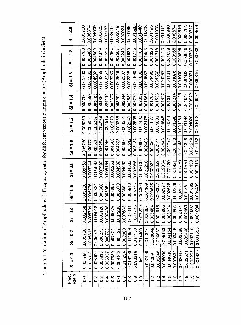
o c

tí o

t i-H

>

H

Si = 2.0

00

II

Si = 1.6

Si = 1.4

Si = 1.2

Si = 1.0

Si = 0.8

Si = 0.6

Si = 0.4

Si = 0.2

Si = 0.0

Freq.

Ratio

0.005760

0.005760

0.005760

0.005760

0.005760

0.005760

0.005760

0.005760

0.005760

0.005760

0.005760

0.0

0.005394

0.005468

0.005536

0.005599

0.005654

0.005703

0.005744

0.005776

0.005799

0.005813

0.005818

0.1

0.004609

0.004800

0.004992

0.005183

0.005367

0.005538

26

99

00

0

0.005821

0.005918

0.005979

0.006000

0.2

0.003825

0.004079

0.004355

0.004651

0.004964

0.005284

0.005599

0.005886

0.006120

0.006275

0.006330

0.3

0.003187

0.003455

0.003762

0.004114

0.004515

0.004966

0.005454

0.005954

0.006408

0.006736

0.006857

0.4

0.002697

0.002954

0.003260

0.003627

0.004070

0.004608

0.005253

0.005997

0.006776

0.007421

0.007680

0.5

0.002319

0.002557

0.002846

0.003204

0.003655

0.004235

0.004992

0.005979

0.007200

0.008427

0.009000

0.6

0.002024

0.002240

0.002507

0.002844

0.003281

0.003866

0.004680

0.005861

0.007605

0.009900

0.011294

0.7

0.001789

0.001985

0.002228

0.002539

0.002949

0.003512

0.004332

0.005618

0.007844

0.011959

0.016000

0.8

0.001598

0.001775

0.001996

0.002279

0.002656

0.003182

0.003966

0.005253

0.007735

0.014150

0.030316

0.9

0.001440

0.001600

0.001800

0.002057

0.002400

0.002880

0.003600

0.004800

0.007200

0.014400

o

0.001308

0.001453

0.001633

0.001866

0.002175

0.002606

0.003250

0.004309

0.006367

0.011814

0.027429

-

0.001195

0.001326

0.001490

0.001700

0.001977

0.002361

0.002924

0.003825

0.005454

0.008846

0.013091

cs!

0.001098

0.001218

0.001366

0.001555

0.001803

0.002141

0.002628

0.003377

0.004615

0.006667

0.008348

cq

0.001014

0.001123

0.001257

0.001427

0.001648

0.001946

0.002364

0.002977

0.003905

0.005183

0.006000

'^

0.000940

0.001039

0.001161

0.001314

0.001511

0.001772

0.002129

0.002628

0.003324

0.004154

0.004608

m

0.000874

99

60

00

0

0.001076

0.001214

0.001390

0.001618

0.001921

0.002328

0.002854

0.003416

0.003692

cp

0.000816

0.000899

0.001000

0.001125

0.001281

0.001481

0.001739

0.002071

0.002474

0.002868

0.003048

h-

0.000764

0.000840

0.000932

0.001044

0.001184

0.001358

0.001579

0.001851

0.002163

0.002448

0.002571

00

0.000717

0.000787

0.000871

0.000972

0.001096

0.001249

0.001438

0.001662

0.001907

0.002119

0.002207

CT>

0.000674

0.000738

0.000815

0.000907

0.001018

0.001152

0.001313

0.001499

0.001694

0.001855

0.001920

2.0

107

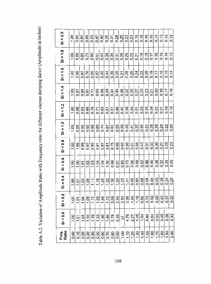
CD

(D

; - i

O

a <D

Si = 2.0

Si = 1.8

Si = 1.6

Si = 1.4

Si = 1.2

Si = 1.0

Si = 0.8

Si = 0.6

Si = 0.4

Si = 0.2

Si = 0.0

Freq.

Ratio

1.00

1.00

1.00

1.00

1.00

1.00

1.00

o q

o q

o q

o q

0.00

0.94

0.95

0.96

0.97

0.98

0.99

1.00

o q

q

q

q

0.10

0.80

0.83

0.87

0.90

0.93

0.96

0.99

q

co q

q

q

0.20

0.66

0.71

0.76

0.81

0.86

0.92

0.97

CM

q

CD

q

q

o

0.30

0.55

0.60

0.65

0.71

0.78

0.86

0.95

CO

q

-

i ^

C55

0.40

0.47

0.51

0.57

0.63

0.71

0.80

0.91

q

00

05 CSj

co co

0.50

0.40

0.44

0.49

0.56

0.63

0.74

0.87

q

0.60

0.35

0.39

0.44

0.49

0.57

0.67

0.81

CM

q

CNI co

CM

CD

q

0.70

0.31

0.34

0.39

0.44

0.51

0.61

0.75

0.98

CD cq

2.08

2.78

0.80

0.28

0.31

0.35

0.40

0.46

0.55

0.69

0.91

• *

cq

2.46

5.26

0.90

0.25

0.28

0.31

0.36

0.42

0.50

0.63

0.83

in CM

2.50

c

o q

0.23

0.25

0.28

0.32

0.38

0.45

0.56

0.75

^

2.05

4.76

1.10

0.21

0.23

0.26

0.30

0.34

0.41

0.51

0.66

0.95

1.54

2.27

o CSI

0.19

0.21

0.24

0.27

0.31

0.37

0.46

0.59

0.80

1.16

1.45

o cq

0.18

0.19

0.22

0.25

0.29

0.34

0.41

0.52

0.68

0.90

1.04

o •51:

0.16

0.18

0.20

0.23

0.26

0.31

0.37

0.46

0.58

0.72

0.80

o

0.15

0.17

0.19

0.21

0.24

0.28

0.33

0.40

0.50

0.59

0.64

o q

0.14

0.16

0.17

0.20

0.22

0.26

0.30

0.36

0.43

0.50

0.53

o

0.13

0.15

0.16

0.18

0.21

0.24

0.27

0.32

0.38

0.43

0.45

o oq

0.12

0.14

0.15

0.17

0.19

0.22

0.25

0.29

0.33

0.37

0.38

o q

0.12

0.13

0.14

0.16

0.20

0.18

0.23

0.26

0.29

0.32

0.33

2.00

108

Table A.3. Variation of Phase Angle with Frequency Ratio (Phase Angle in degrees)

Freq. Ratio

0.0 0.1 0.2 0.3 0.4 0.5 0.6 0.7 0.8 0.9 1.0 1.1 1.2 1.3 1.4 1.5 1.6 1.7 1.8 1.9 2.0 2.1 2.2 2.3 2.4 2.5 2.6 2.7 2.8 2.9 3.0

Si = 0.05

0 1 1 2 3 4 5 8 13 25 90 152 165 169 172 173 174 175 175 176 176 176 177 177 177 177 177 178 178 178 178

Si = 0.25

0 3 6 9 13 18 25 34 48 67 90 111 126 137 144 149 153 156 158 160 162 163 164 165 166 167 167 168 168 169 169

Si = 0.1

0 1 2 4 5 8 11 15 24 43 90 134 151 159 164 167 168 170 171 172 172 173 173 174 174 175 175 175 175 176 176

Si = 0.5

0 6 12 18 25 34 43 54 66 78 90 101 110 118 124 130 134 138 141 144 146 148 150 152 153 155 156 157 158 159 159

Si = 1.0

0 11 23 33 44 53 62 70 77 84 90 95 100 105 109 113 116 119 122 124 127 129 131 133 135 136 138 139 141 142 143

Si = 2.0

0 22 40 53 62 69 75 80 84 87 90 93 95 98 100 102 104 106 107 109 111 112 114 115 116 118 119 120 121 123 124

Si = 3.0

0 31 51 63 71 76 80 83 86 88 90 92 93 95 97 98 99 100 102 103 104 105 106 107 108 109 110 111 112 113 114

Si = 4.0

0 42 62 71 77 81 83 85 87 89 90 91 92 93 94 95 96 97 98 99 99 100 101 102 102 103 104 105 105 106 107

Si = 5.0

0 45 64 73 78 81 84 86 87 89 90 91 92 93 94 95 96 96 97 98 99 99 100 101 101 102 102 103 104 104 105

109

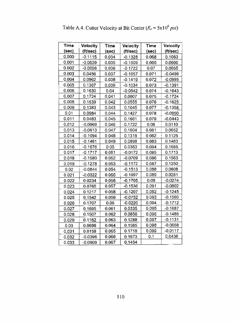
Table A.4. Cutter Velocity at Bit Center (Er = 5x\&psi)

Time (sec) 0.000 0.001 0.002 0.003 0.004 0.005 0.006 0.007 0.008 0.009 0.01

0.011 0.012 0.013 0.014 0.015 0.016 0.017 0.018 0.019 0.02

0.021 0.022 0.023 0.024 0.025 0.026 0.027 0.028 0.029 0.03

0.031 0.032 0.033

Velocity (ft/sec) -0.1115 -0.0639 -0.0096 0.0456 0.0962 0.1367 0.1630 0.1724 0.1639 0.1383 0.0984 0.0483 -0.0069 -0.0613 -0.1094 -0.1461 -0.1676 -0.1717 -0.1580 -0.1278 -0.0844 -0.0322 0.0234 0.0765 0.1217 0.1542 0.1707 0.1695 0.1507 0.1162 0.0696 0.0158 -0.0396 -0.0909

Time (sec) 0.034 0.035 0.036 0.037 0.038 0.039 0.04

0.041 0.042 0.043 0.044 0.045 0.046 0.047 0.048 0.049 0.05

0.051 0.052 0.053 0.054 0.055 0.056 0.057 0.058 0.059 0.06

0.061 0.062 0.063 0.064 0.065 0.066 0.067

Velocity (ft/sec) -0.1328 -0.1609 -0.1722 -0.1657 -0.1419 -0.1034 -0.0542 0.0007 0.0555 0.1045 0.1427 0.1661 0.1722 0.1604 0.1319 0.0898 0.0383 -0.0172 -0.0709 -0.1172 -0.1513 -0.1697 -0.1705 -0.1536 -0.1207 -0.0752 -0.0220 0.0335 0.0856 0.1288 0.1585 0.1718 0.1673 0.1454

Time (sec) 0.068 0.069 0.07

0.071 0.072 0.073 0.074 0.075 0.076 0.077 0.078 0.079 0.08

0.081 0.082 0.083 0.084 0.085 0.086 0.087 0.088 0.089 0.09

0.091 0.092 0.093 0.094 0.095 0.096 0.097 0.098 0.099

0.1

Velocity (ft/sec) 0.1083 0.0600 0.0055 -0.0496 -0.0995 -0.1391 -0.1643 -0.1724 -0.1625 -0.1358 -0.0950 -0.0443 0.0110 0.0652 0.1126 0.1483 0.1685 0.1713 0.1563 0.1250 0.0808 0.0281 -0.0274 -0.0802 -0.1245 -0.1560 -0.1712 -0.1687 -0.1486 -0.1131 -0.0658 -0.0117 0.0436

110

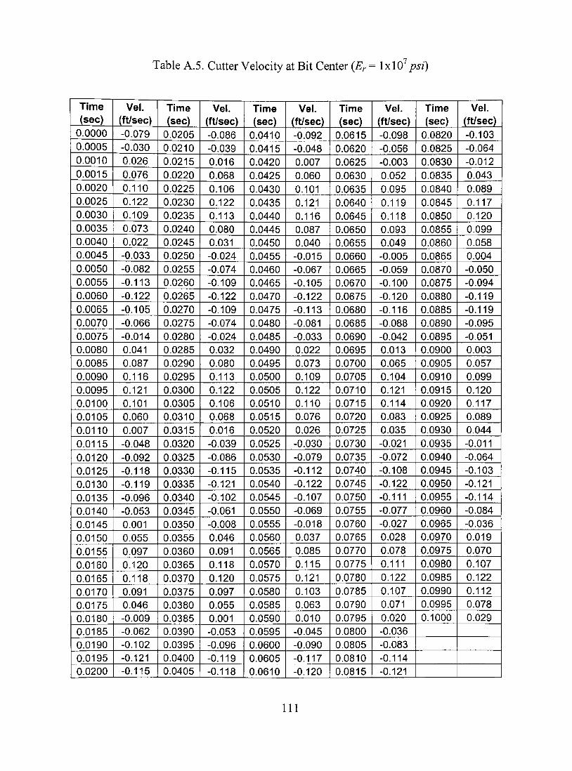
Table A.5. Cutter Velocity at Bit Center (Er = \y.\0'psi)

Time (sec)

0.0000 0.0005 0.0010 0.0015 0.0020 0.0025 0.0030 0.0035 0.0040 0.0045 0.0050 0.0055 0.0060 0.0065 0.0070 0.0075 0.0080 0.0085 0.0090 0.0095 0.0100 0.0105 0.0110 0.0115 0.0120 0.0125 0.0130 0.0135 0.0140 0.0145 0.0150 0.0155 0.0160 0.0165 0.0170 0.0175 0.0180 0.0185 0.0190 0.0195 0.0200

Vel. (ft/sec) -0.079 -0.030 0.026 0.076 0.110 0.122 0.109 0.073 0.022 -0.033 -0.082 -0.113 -0.122 -0.105 -0.066 -0.014 0.041 0.087 0.116 0.121 0.101 0.060 0.007 -0.048 -0.092 -0.118 -0.119 -0.096 -0.053 0.001 0.055 0.097 0.120 0.118 0.091 0.046 -0.009 -0.062 -0.102 -0.121 -0.115

Time (sec)

0.0205 0.0210 0.0215 0.0220 0.0225 0.0230 0.0235 0.0240 0.0245 0.0250 0.0255 0.0260 0.0265 0.0270 0.0275 0.0280 0.0285 0.0290 0.0295 0.0300 0.0305 0.0310 0.0315 0.0320 0.0325 0.0330 0.0335 0.0340 0.0345 0.0350 0.0355 0.0360 0.0365 0.0370 0.0375 0.0380 0.0385 0.0390 0.0395 0.0400 0.0405

Vel. (ft/sec) -0.086 -0.039 0.016 0.068 0.106 0.122 0.113 0.080 0.031 -0.024 -0.074 -0.109 -0.122 -0.109 -0.074 -0.024 0.032 0.080 0.113 0.122 0.106 0.068 0.016 -0.039 -0.086 -0.115 -0.121 -0.102 -0.061 -0.008 0.046 0.091 0.118 0.120 0.097 0.055 0.001 -0.053 -0.096 -0.119 -0.118

Time (sec)

0.0410 0.0415 0.0420 0.0425 0.0430 0.0435 0.0440 0.0445 0.0450 0.0455 0.0460 0.0465 0.0470 0.0475 0.0480 0.0485 0.0490 0.0495 0.0500 0.0505 0.0510 0.0515 0.0520 0.0525 0.0530 0.0535 0.0540 0.0545 0.0550 0.0555 0.0560 0.0565 0.0570 0.0575 0.0580 0.0585 0.0590 0.0595 0.0600 0.0605 0.0610

Vel. (ft/sec) -0.092 -0.048 0.007 0.060 0.101 0.121 0.116 0.087 0.040 -0.015 -0.067 -0.105 -0.122 -0.113 -0.081 -0.033 0.022 0.073 0.109 0.122 0.110 0.076 0.026 -0.030 -0.079 -0.112 -0.122 -0.107 -0.069 -0.018 0.037 0.085 0.115 0.121 0.103 0.063 0.010 -0.045 -0.090 -0.117 -0.120

Time (sec)

0.0615 0.0620 0.0625 0.0630 0.0635 0.0640 0.0645 0.0650 0.0655 0.0660 0.0665 0.0670 0.0675 0.0680 0.0685 0.0690 0.0695 0.0700 0.0705 0.0710 0.0715 0.0720 0.0725 0.0730 0.0735 0.0740 0.0745 0.0750 0.0755 0.0760 0.0765 0.0770 0.0775 0.0780 0.0785 0.0790 0.0795 0.0800 0.0805 0.0810 0.0815

Vel. (ft/sec) -0.098 -0.056 -0.003 0.052 0.095 0.119 0.118 0.093 0.049 -0.005 -0.059 -0.100 -0.120 -0.116 -0.088 -0.042 0.013 0.065 0.104 0.121 0.114 0.083 0.035 -0.021 -0.072 -0.108 -0.122 -0.111 -0.077 -0.027 0.028 0.078 0.111 0.122 0.107 0.071 0.020 -0.036 -0.083 -0.114 -0.121

Time (sec)

0.0820 0.0825 0.0830 0.0835 0.0840 0.0845 0.0850 0.0855 0.0860 0.0865 0.0870 0.0875 0.0880 0.0885 0.0890 0.0895 0.0900 0.0905 0.0910 0.0915 0.0920 0.0925 0.0930 0.0935 0.0940 0.0945 0.0950 0.0955 0.0960 0.0965 0.0970 0.0975 0.0980 0.0985 0.0990 0.0995 0.1000

Vel. (ft/sec) -0.103 -0.064 -0.012 0.043 0.089 0.117 0.120 0.099 0.058 0.004 -0.050 -0.094 -0.119 -0.119 -0.095 -0.051 0.003 0.057 0.099 0.120 0.117 0.089 0.044 -0.011 -0.064 -0.103 -0.121 -0.114 -0.084 -0.036 0.019 0.070 0.107 0.122 0.112 0.078 0.029

111

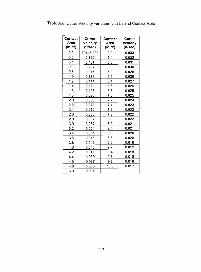
Table A.6. Cutter Velocity variation with Lateral Contact Area

Contact Area

(in**2)

0.0 0.2 0.4 0.6 0.8 1.0 1.2 1.4 1.6 1.8 2.0 2.2 2.4 2.6 2.8 3.0 3.2 3.4 3.6 3.8 4.0 4.2 4.4 4.6 4.8 5.0

Cutter Velocity (ft/sec)

70147.222 0.862 0.431 0.287 0.216 0.172 0.144 0.123 0.108 0.096 0.086 0.078 0.072 0.066 0.062 0.057 0.054 0.051 0.048 0.045 0.043 0.041 0.039 0.037 0.036 0.034

Contact Area

(in**2)

5.2 5.4 5.6 5.8 6.0 6.2 6.4 6.6 6.8 7.0 7.2 7.4 7.6 7.8 8.0 8.2 8.4 8.6 8.8 9.0 9.2 9.4 9.6 9.8 10.0


0.033 0.032 0.031 0.030 0.029 0.028 0.027 0.026 0.025 0.025 0.024 0.023 0.023 0.022 0.022 0.021 0.021 0.020 0.020 0.019 0.019 0.018 0.018 0.018 0.017

112

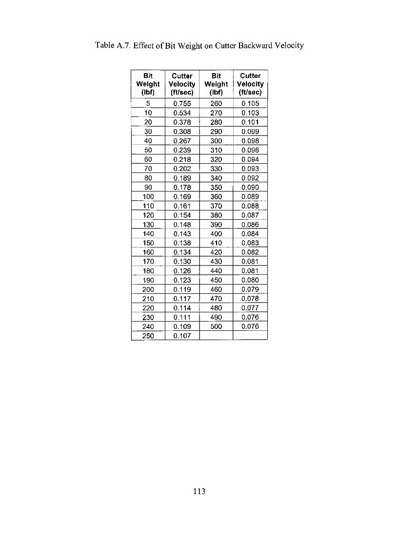
Table A.7. Effect of Bit Weight on Cutter Backward Velocity

Bit Weight

(Ibf)

5 10 20 30 40 50 60 70 80 90 100 110 120 130 140 150 160 170 180 190 200 210 220 230 240 250


0.755 0.534 0.378 0.308 0.267 0.239 0.218 0.202 0.189 0.178 0.169 0.161 0.154 0.148 0.143 0.138 0.134 0.130 0.126 0.123 0.119 0.117 0.114 0.111 0.109 0.107

Bit Weight

(Ibf)

260 270 280 290 300 310 320 330 340 350 360 370 380 390 400 410 420 430 440 450 460 470 480 490 500


0.105 0.103 0.101 0.099 0.098 0.096 0.094 0.093 0.092 0.090 0.089 0.088 0.087 0.086 0.084 0.083 0.082 0.081 0.081 0.080 0.079 0.078 0.077 0.076 0.076

113

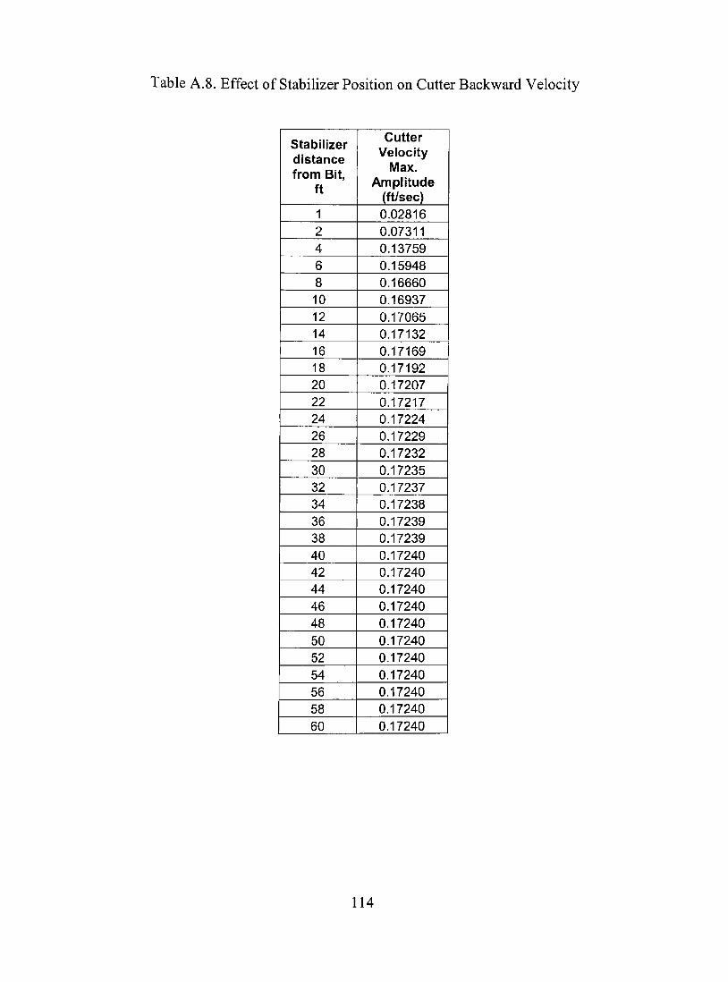
Table A.8. Effect of Stabihzer Position on Cutter Backward Velocity

Stabilizer distance from Bit,

ft

1 2 4 6 8 10 12 14 16 18 20 22 24 26 28 30 32 34 36 38 40 42 44 46 48 50 52 54 56 58 60

Cutter Velocity

Max. Amplitude

(ft/sec) 0.02816 0.07311 0.13759 0.15948 0.16660 0.16937 0.17065 0.17132 0.17169 0.17192 0.17207 0.17217 0.17224 0.17229 0.17232 0.17235 0.17237 0.17238 0.17239 0.17239 0.17240 0.17240 0.17240 0.17240 0.17240 0.17240 0.17240 0.17240 0.17240 0.17240 0.17240

114

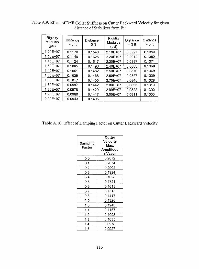
Table A.9. Effect of Drill Collar Stifíhess on Cutter Backward Velocity for given distance of Stabihzer from Bit

Rigidity Modulus

(psi)

1.00E+07 1.10E+07 1.15E+07 1.30E+07 1.40E+07 1.50E+07 1.60E+07 1.70E+07 1.80E+07 1.90E+07 2.00E+07

Distance = 3ft

0.1170 0.1140 0.1124 0.1085 0.1061 0.1038 0.1017 0.0997 0.0978 0.0960 0.0943

Distance = 5ft

0.1540 0.1525 0.1517 0.1496 0.1482 0.1468 0.1455 0.1442 0.1429 0.1417 0.1405

Rigidity IViodulus

(psi)

2.10E+07 2.20E+07 2.30E+07 2.40E+07 2.50E+07 2.60E+07 2.70E+07 2.80E+07 2.90E+07 3.00E+07

Distance = 3ft

0.0927 0.0912 0.0897 0.0883 0.0870 0.0857 0.0845 0.0833 0.0822 0.0811

Distance = 5ft

0.1393 0.1382 0.1371 0.1360 0.1349 0.1339 0.1329 0.1319 0.1309 0.1300

Table A.IO. Effect of Damping Factor on Cutter Backward Velocity

Damping Factor

0.0 0.1 0.2 0.3 0.4 0.5 0.6 0.7 0.8 0.9 1.0 1.1 1.2 1.3 1.4 1.5

Cutter Velocity

Max. Amplitude

(ft/sec) 0.2072 0.2054 0.2002 0.1924 0.1828 0.1724 0.1618 0.1515 0.1417 0.1326 0.1243 0.1167 0.1098 0.1035 0.0978 0.0927

115

APPENDIX B

MATLAB SOURCE CODE

116

B.l

%MATLAB program to calculatc the valucs of íiuictions S(x), r(x), U(x), F(x). G(x).

H(x). P(x), Q(x). R(x)

clc;clearan;pl=l;xl=0.0:-0.01:-6.0;xl=xl';

forx-0.0:-0.01:-6.0

sxl=l;sx2=l;sumsx=0;txl=l;tx2=l;sumtx=0;uxl=l;ux2=l;sumux=0;

fxl=l;fx2=l;sum6c=0;gxl=l;gx2=l;sumgx=0;hxl=l;hx2=l;sumhx=0;

pxl=l;px2=l;sumpx=0;qxl=l;qx2=l;sumqx=0;rxl=l;rx2=l;sumrx=0;

forn=l:50

sxl=l;sx2=l;txl=l;tx2=l;uxl=l;ux2=l;fxl=l;fx2=l;gxl=l;gx2=l;hxl=l;hx2=l;

pxl=l;px2=l;qxl=l;qx2=l;rxl=l;rx2=l;

if n==l % initializing the first terms of diffcrent series to individua! variables

sumsxl=x;sumtxl=0.5*x^2;sumuxl=-x'^3/6.0;sumfxl=L0;sumgxl=x;

sumhxl=-x^2/2.0;sumpxl=-x'*^2/2.0;sumqxl=1.0;sumrxl=-x;

sumsx=sumsx+sumsx 1 ;sumtx=sumtx+sumtx 1 ;sumux=sumux+sumux 1;

sumfx=sumfx+sumfxl ;sumgx=sumgx+sumgxl ;sumhx=sumhx+sumhxl;

sumpx=sumpx+sumpxl ;sumqx=sumqx+sumqxl ;sumrx=sumrx+sumrxl;

else

ifn==2 sumqx 1 -x'^S/S.0;sumqx=sumqx+sumqx 1;

else

numqx=(-l)'^(n+l)*x'^(3*n-3);pqx=3*n-3;nqxterms=2*n-4;nqxl=nqxterms/2;

foril=l:nqxl qxl=3*il*qxl;qx2=(3*il+l)*qx2; end

sumqx 1 =numqx/(pqx*qx 1 );sumqx 1 =sumqx l/qx2;sumqx=sumqx+sumqx 1;

end

% the following lines evakiates the values of powers of x each tenn of the

individual functions

numsx^í-l^^ín-l^^x'^^^^n-^^^numtxK-l^^^n-l^^x^^^^n-l^^numux^^-l^^n^x^^^^n);

numfx=(-l)^(n+l)*x^(3*n-3);numgx=(-l)^(n-l)*x^(3*n-2);

numhx=(-1 )^n*x^(3 *n-1) ;numpx=(-1 ) n*x'* (3 *n-1 );numrx=(-1 ' n^x^^^ *n-2);

117

psx=3*n-2;ptx=3*n-l;pux=3*n;nsxterms=2*n-l;ntxtenns-2*n-2;nuxterms=2*n-2;

nf?cterms=2*n-2;ngxterms=2*n-2;nhxterms=2*n-2;npxterms=2*n-2;

nrxterms=2*n-2;

nsx 1 =(nsxterms-1 )/2 ;ntx 1 =ntxterms/2 ;nux 1 =nuxterms/2;

nfx 1 =nfxterms/2 ;ngx 1 =ngxterms/2 ;nhx 1 =nhxterms/2;

npx 1 =npxterms/2 ;nrx 1 =nrxterms/2;

% the following conditional statements evaluates the integers in each term of

Ihe denominators

foril=l:nsxl sxl=(3*il-l)*sxl;sx2=3*il*sx2;end

foril=l:ntxl txl=3*il*txl;tx2=(3*il+l)*tx2;end

foril=l:nuxl uxl=(3*il+l)*uxl;ux2=(3*il+2)*ux2;end

foril=l:nfxl fxl=(3*il-l)*fxl;fx2=3*il*fe2;end

foril=l:ngxl gxl=3*il*gxl;gx2=(3*il+l)*gx2;end

foril=l:nhxl hxl=(3*il+l)*hxl;hx2=(3*il+2)*hx2;end

foril=l:npxl pxl=3*il*pxl;px2=(3*il+2)*px2;end

for il=l:nrxl rxl=(3*il-l)*rxl;rx2=(3*il+l)*rx2;end

% the following lines sums the individual terms in the series for each function

sumsx 1 =numsx/(sx 1 *psx);sumtx 1 =numtx/(tx 1 *ptx);sumux 1 =numux/(2*ux 1 *pux);

sumfx 1 =numfx/fx 1; sumgx 1 =numgx/gx 1; sumhx 1 =numhx/(2 *hx 1);

sumpx 1 =numpx/(2*px 1 );sumrx 1 =numrx/rx 1;

sumsx 1 =sumsx 1 /sx2; sumtx 1=sumtx 1 /tx2; sumux 1=sumux 1 /ux2;

sumfx 1 =sumfx 1/fx2; sumgx 1 =sumgx 1/gx2; sumhx 1 =sumhx 1/hx2;

sumpx 1 =sumpx 1 /px2; sumrx 1 =sumrx 1 /rx2;

% the following three lines represení the fmal values of the each function for given

values of x

sumsx=sumsx+sumsxl ;sumtx=sumtx+sumtxl ;sumux=sumux+sumuxl;

sumfx=sumfx:+sumfx 1 ;sumgx=sumgx+sumgx 1 ;sumhx=sumhx+sunihx 1;

sumpx=sumpx+sumpx 1 ;sumrx=sumrx+sumrx 1;

end

118

end

sx(pl)=sumsx;tx(pl)=sumtx;ux(pl)=sumux;fx(pl)=sumfx;gx(pl)=sumgx;

hx(p 1 )=sumhx;px(p 1 )=sumpx;qx(p 1 )=sumqx;rx(p 1 )=sumrx; p 1 =p 1+1

end

sx=sx';sxo=[xl,sx];tx=tx';txo=[xl,tx];ux=ux';uxo=[xl,ux];fx=fx';fxo=[xLfx];gx=gx':

gxo=[x 1 ,gx] ;hx=hx';hxo=[x 1 ,hx] ;px=px';pxo=[x 1 ,px] ;qx=qx';qxo=[x 1 ,qx] ;rx=rx';

rxo=[xl,rx];

% the values of each fimction for given values of x are stored in individual text ííles

showii below

saveCsx.txtVsxoV-ascii');save('tx.txtVtxo','-ascii');save('ux.txtVuxoV-ascii');

save(*fx.txtVfxo','-ascii');save('gx.txt','gxo','-ascii');save('hx.txtVhxo','-ascii');

save('px.txt','pxo','-ascii');save('qx.txt','qxo','-ascii');save('rx.txt','rxo','-ascii');

119

B.2

%MATLAB program to calculate thc value of xl and x2 and write data to a text fíle

clc;clearall;pl=l;st=2.7;il=st:-0.0001:0.0;i2=size(il,2);

for i=0.0:-0.2:-8.0 % the values of i rcfer to values of xl

[csx,ctx,cux,cfx,cgx,chx,cpx,cqx,crx]=call_det(i); % value of individual functions for

dilTerent values of i are evaluated by calling the subroutine

sxl(pl)=csx;txl(pl)=ctx;uxl(pl)=cux;6cl(pl)=cfx; % initializing variables

gxl(pl)=cgx;hxl(pl)=chx;pxl(pl)=cpx;qxl(pl)=cqx;rxl(pl)=crx;

q=i;

forxl=st:-0.0001:1.7

[csx,ctx,cux,cfx,cgx,chx,cpx,cqx,crx]=call_det(xl); % value of individual functions

for different values of xl are evaluated by calling the subroutine

a=[pxl(pl),qxl(pl),rxl(pl);cpx,cqx,crx;sxl(pl)-csx,txl(pl)-ctx,uxl(pl)-cux];

al(q)=det(a);bl(q)=xl; % determinant is evaluated

if xl==st gl=abs(al(l));hl=bl(l); % condition to check forthe lowest absolute

value of the determinant

else if abs(al(q))<=gl gl=abs(al(q));hl=bl(q); end

end

q=q+l;

end

cxl(pl)=i;cx2(pl)=hl;c_err(pl)=gl;fprintf('\n%8.5f%8,5f%8.5f,i,hl,gl);

pl=pl+l;

end

cxl=cxl';cx2=cx2';c_err=c__err*;b=[cxl,cx2,c_err];save('ccl.txt','b','-ascii');

% subroutine evaluated below and the individual values of function determined

% the subroutine program is similar to the program shown in section B-1

function [sxf,txf,uxf,fxf,gxf,hxf,pxf,qxf,rxf]=call_det(xf)

sxl=l;sx2=l;sumsx=0;txl=l;tx2=l;sumtx=0;uxl=l;ux2=l;sumux=0;

fxl=l;fx2=l;sumfx=0;gxl=l;gx2=l;sumgx=0;hxl=l;hx2=l;sumhx=0;

120

pxl=l;px2=l;sumpx=0;qxl=l;qx2=l;sumqx=0;rxl=l;rx2=l;sumrx=0;

forn=l:20 sxl=l;sx2=l;txl=l;tx2=l;uxl=l;ux2=l;

fxl=l;fx2=l;gxl=l;gx2=l;hxl=l;hx2=l;pxl=l;px2=l;qxl=l;qx2=l;ncl=l;rx2=l;

ifn==l sumsxl=xf;sumtxl=0.5*xf^2;sumuxl=-xf^3/6.0;

sumfxl=1.0;sumgxl=xf;sumhxl=-xf'^2/2.0;

sumpxl=-xf^2/2.0;sumqxl=1.0;sumrxl=-xf;


sumfx=sumfx+sumfx 1 ;sumgx=sumgx+sumgx 1 ;sumhx=sumhx+sumhx 1;

sumpx=sumpx+sumpx 1 ;sumqx=sumqx+sumqx 1 ;sumrx=sumrx+sumrx 1;

eise

if n==2 sumqxl=-xf^3/3.0;sumqx=sumqx+sumqxl;

else

numqx=(-l)'^(n+l)*xf'^(3*n-3);pqx=3*n-3;nqxterms=2*n-4;nqxl=nqxterms/2;

for il=l:nqxl qxl=3*il*qxl;qx2=(3*il+l)*qx2;end

sumqx 1 =numqx/(pqx*qx 1 );sumqx 1 =sumqx 1 /qx2;sumqx=sumqx+sumqx 1;

end

numsx=(-l)^(n-l)*xf^(3*n-2);numtx=(-l)^(n-l)*xf^(3*n-l);

numux=(-1 n xf' ^ *n);

numfx=(-l)^(n+l)*xf^(3*n-3);numgx=(-l)^(n-l)*xf^(3*n-2);

numhx=(-l)^n*xf^(3*n-l);numpx=(-l)^n*xf^(3*n-l);numrx=(-l)^n*xf^(3*n-2);

psx=3*n-2;ptx=3*n-l;pux=3*n; nsxterms=2*n-l;ntxterms=2*n-2;nuxterms=2*n-2;

nfxterms=2*n-2;ngxterms=2*n-2;nlixterms=2*n-2; npxterms=2*n-2;

nrxterms=2 *n-2; nsx 1 =(nsxterms-1 )/2 ;ntx 1 =ntxterms/2;nux 1 =nuxterms/2;

nfx 1 =nfxterms/2 ;ngx 1 =ngxterms/2 ;nhx 1 =nhxterms/2;

npx 1 =npxterms/2;nrx 1 =nrxterms/2;

foril=l:nsxl sxl=(3*il-l)*sxl;sx2=3*il*sx2;end

foril=l:ntxl txl=3*il*txl;tx2=(3*il+l)*tx2;end

foril=l:nuxl uxl=(3*il+l)*uxl;ux2=(3*il+2)*ux2;end

foril=l:nfxl fxl=(3*il-l)*fxl;fx2=3*il*fx2;end

121

foril=l ngxl gxl=3*il*gxl;gx2=(3*il+l)*gx2;end

foril=l:nhxlhxl=(3*il+l)*hxl;hx2=(3*il+2)*hx2;end

foril=l:npxl pxl=3*il*pxl;px2=(3*il+2)*px2;end

foril=l:nrxlrxl=(3*il-l)*rxl;rx2=(3*il+l)*rx2;end

sumsx 1 =numsx/(sx 1 *psx);sumtx 1 =numtx/(tx 1 *ptx);sumux 1 =numux/(2*ux 1 *pux);

sumfx 1 =numfx/fxl ;sumgx 1 =numgx/gx 1 ;sumhx 1 =numhx/(2*hx 1);

sumpx 1 =numpx/(2 *px 1); sumrx 1 =numrx/rx 1;

sumsx 1 =sumsx 1 /sx2; sumtx 1=sumtx 1 /tx2; sumux 1 =sumux 1 /ux2;

sumfx 1 =sumfx 1/fx2; sumgx 1=sumgx 1/gx2; sumhx 1 =sumhx 1/hx2;

sumpx 1 =sumpx 1 /px2; sumrx 1=sumrx 1 /rx2;


sumfx=sumfx:+sumfx 1 ;sumgx=sumgx+sumgx 1 ;sumhx=sumhx+sumhx 1;

sumpx=sumpx+sumpx 1 ;sumrx=sumrx+sumrx 1;

end

end

sxf=sumsx;txf=sumtx;uxf=sumux; fxf=sumfx;gxf^sumgx;hxf=sumhx;

pxf=sumpx;qxf=sumqx;rxf=sumrx;

retum

122

B.3

%MA'ri.AB program for calculating the tangcncy point x3 for fírst order critical

buckiing

clc; clear all

pl=l;st=L94;

[csx,ctx,cux,cfx,cgx,chx,cpx,cqx,crx]=call_det(-6.0); %function values evaluated by

calhng subroutine. Subroutine program hsted in section B-2.

sxl=csx;txl=ctx;uxl=cux;fxl=cfx;

gxl=cgx;hxl=chx;pxl=cpx;qxl=cqx;rxl=crx;

[csx,ctx,cux,cfx,cgx,chx,cpx,cqx,crx]=call_det(1.94);

sx2=csx;tx2=ctx;ux2=cux;fx2=cfx;

gx2=cgx;hx2=chx;px2=cpx;qx2=cqx;rx2=crx;

for i=st:-0.0001:0.0 % this if statement evaluates the determinant and checks for the

lowest absolute value of the detemiinant

[csx,ctx,cux,cfx,cgx,chx,cpx,cqx,crx]=call_det(i);

a=[cfx,cgx,chx;px 1 ,qx 1 ,rx 1 ;px2,qx2,rx2]; al (p 1 )=det(a);b 1 (p 1 )=i;

if i==st gl=abs(al(l));hl=bl(l);

else

if abs(al(pl))<-gl gl=abs(al(pl));hl=bl(pl); end

end

pi=pi+i;

end

fjprintf('\nThe Value of X3 =%8.5f ,hl); % the distance between the neutral point and

taiigency point is determined.

123

R 4

%MATl.AB program to calculate thc value of x2 when the second bucklc contacts the

borehole wall

clc;clear all

wt=input('Weight per unit length of Drill-Collars (Ib/ft):');

e=input('Elastic Modulus (lbf/in**2):');

od=input('Drill Colkir O.D (in.):');

id=input('Drill-Collar I.D (in.):');

hdia=input('Dia. of Hole (in.):');

mi=pi*(odM-idM)/(12M*64.0);m=(e*144*mi/wt)^0.3333; % calculates moment of

inertia of drill collar and lcngth of one dimcnsionless unit of drill collar

r=(hdia-od)/(2.0* 12);x2=4.1:0.001:4.5;x2=x2';

[csxl,ctxl,cuxl,cfxl,cgxl,chxl,cpxl,cqxl,crxl]=call_det(-6.0); % subroutine evaluated

for xl =-6.0 and values of diflerent functions determined. Subroutine listed in section B-2

% the ibllowing for statements are evaluated in loop until ibr a particular value of i2, ihe

determinant is equal to the lowest possible absolute value. This value of i2 equals to the

value of x2 when the second buckle contacts the bore hole w'all.

for i2=l:size(x2,l) q=l;dl=[];el=[];st=3.0;

[Csx2,ctx2,cux2,cfx2,cgx2,chx2,cpx2,cqx2,crx2]=call_det(x2(i2));

forx3=st:0.0001:3.2

[csx3,ctx3,cux3,cfx3,cgx3,chx3,cpx3,cqx3,crx3]=call_det(x3);

a=[cpxl,cqxl,crxl,0.0,0.0,0.0,0.0;cf c3,cgx3,chx3,0.0,0.0,0.0,0.0;...

(csx3-csxl),(ctx3-ctxl),(cux3-cuxl),0.0,0.0,0.0,r/m;...

0.0,0.0,0.0,cpx2,cqx2,crx2,0.0;...

0.0,0.0,0.0,cfx3,cgx3,chx3,0.0;0.0,0.0,0.0,(csx3-csx2),(ctx3-ctx2),(cux3-

cux2),r/m; cpx3,cqx3,crx3,-cpx3,-cqx3,-crx3,0.0];

dl(q)=det(a);el(q)=x3;

if abs(dl(q))<=0.01 gl=abs(dl(q));hl=el(q);i2=size(x2,l)+l; break; end

q=q+l; end end

124

B.5

/oMA IT..AB program to calculate the equation coefficients, values of x2, x3 and thc force

coeffícient f

clc; clear all

wt=input('Weight per unit length of Drill-Collars (Ib/ft):');

e=input('EIastic Modulus (Ibf/in**2):');

od=input('Drill Colkir O.D (in.):');

id=input('DriII-Collar I.D (in.):');


mi=pi*(od^4-idM)/(12M*64.0); m=(e* 144*^1/^^)^^0.3333;

r=(hdia-od)/(2.0*12);x2=[1.94,2.0,2.3,2.6,3.2,3.5,3.753,4.0,4.1,4.218]';

pl=l;xl=-6.0;st=0.0;il=size(x2,l);

[csxl,ctxl,cuxl,cf!íl,cgxl,chxl,cpxl,cqxl,crxl]=caII_det(-6.0); %function value at xl==-

6.0 evaluated by calling subroutine.

sx 1 =csx 1 ;tx 1 =ctx 1 ;ux 1 =cux 1 ;fx 1 =cfx 1;

gx 1 =cgx 1 ;hx 1 =chx 1 ;px 1 =cpx 1 ;qx 1 =cqx 1 ;rx 1 =crx 1;

% the following for statements are evaluated in loop until for a particular value of i, the

determinant is equal to the lowest possible absokite value.

fori=l:il

[csx(i),ctx(i),cux(i),cfx(i),cgx(i),chx(i),cpx(i),cqx(i),crx(i)]=call_det(x2(i));

q=l;

forx3=st:0.0001:st+l

[Csx3,ctx3,cux3,cfx3,cgx3,chx3,cpx3,cqx3,crx3]=call_det(x3);

a=[pxl,qxl,rxl,0.0,0.0,0.0,0.0;cfx3,cgx3,chx3,0.0,0.0,0.0,0.0;...

(csx3-sxl),(ctx3-txl),(cux3-uxl),0.0,0.0,0.0,r/m;...

O.0,O.O,0.O,cpx(i),cqx(i),crx(i),0.O;.O,0.0,O.0,cfx3,cgx3,chx3,0.O;...

0.0,0.0,0.0,(csx3-csx(i)),(ctx3-ctx(i)),(cux3-cux(i)),r/m;...

cpx3,cqx3,crx3,-cpx3,-cqx3,-crx3,0.0];


125

ifabs(dl(q))<=0.01 gl=abs(dl(q));hl=el(q); break; end

q=q+i;

end

cx2(pl)=x2(i);cx3(pl)=hl;c_err(pl)=gl;st=cx3(pl);

% the values of the coefficients al. bl, cl and a2. b2, c2 from the simultaneous

equations are determined

Cl(i)=l/((csx3-sxl)*(qxl*chx3-cgx3*rxl)/(pxl*cgx3-cfx3*qxl)+(cux3-uxl)+...

(Ctx3-txl)*(rxl*cfx3-pxl*chx3)/(pxl*cgx3-cfx3*qxl));

al(i)=(qxl*chx3-cgx3*rxl)*cl(i)/(pxl*cgx3-cfx3*qxl);

bl(i)=(rxl*cfx3-pxl*chx3)*cl(i)/(pxl*cgx3-cfx3*qxl);

C2(i)=l/((csx3-csx(i))*(cqx(i)*chx3-cgx3*crx(i))/(cpx(i)*cgx3-cfx3*cqx(i))+...

(cux3-cux(i))+(ctx3-ctx(i))*(crx(i)*cfx3-chx3*cpx(i))/(cpx(i)*cgx3-cfx3*cqx(i))):

a2(i)=(cqx(i)*chx3-cgx3*crx(i))*c2(i)/(cpx(i)*cgx3-cfx3*cqx(i));

b2(i)=(crx(i)*cfx3-chx3*cpx(i))*c2(i)/(cpx(i)*cgx3-cfx3*cqx(i));

f(i)=c2(i)*m/r-cl(i)*m/r; % the force coefllcient is determined

^rintf('\n%8.5f%8.5f%8.5f,x2(i),hl,gl);

^rintf('\n%8.5f%8.5f%8.5f%8.5f%8.5f%8.5f

%8.5f,x2(i),al(i),bl(i),cl(i),a2(i),b2(i),c2(i));

pl=pl+l;

end

cx2=cx2';cx3=cx3';c_err=c_err';f=f;

al=al';bl=br;cl=cr;a2=a2';b2=b2';c2=c2';

tl=[cx2,cx3,c_err]; t2=[al,bl,cl,a2,b2,c2];t3=[x2,f];

% the values of x2 and x3, the coefílcients (al, bl, cl, a2, b2, c2) and the íbrce

cocfflcients data variation with x2 are stored in respective fllcs below.

save('cc2_tl.txt','tl','-ascii');save('cc2_t2.txt','t2','-ascii');save('f_value.txt','t3','-ascii');

126

R6

AMAITAB program for calculating the x-y values for dctennining shapc of buckled

dnlling string and bending moment coefficients for fîrst and higher buckling orders

clc; clear all

wt=input('Weight per unit length of Drill-CoUars (Ib/ft):');

e=input('EIastic Modulus (Ibf/in**2):');

od=input('Drill CoIIai- O.D (in.):');

id=input('DriII-Collar I.D (in.):');


mi=pi*(odM-idM)/(12M*64.0);m=(e*144*mi/wt)^0.3333;

r=(hdia-od)/(2.0*12);x2=[1.94,3.753,4.219]';

[csxl,ctxl,cuxl,cfxl,cgxl,chxl,cpxl,cqxl,crxl]=caIl_det(-6.0); % function values at

xl==-6.0 determined by calling subroutine

for i2=l:3 q=l;x4=-x2(i2)-6.0;dl=[];el=[];

x=x2(i2):-0.1:x4;x=x'; il=size(x,l);

[Csx2,ctx2,cux2,cfx2,cgx2,chx2,cpx2,cqx2,crx2]=call_det(x2(i2)); %llinction values

evaluated at different values of x2, i.e.1.94, 3.753, 4.219, by calling subroutine

if i2==l st=0.0; elseif i2==2 st=2.0; elseif i2==3 st=3.0; end

for x3=st:0.0001:x2(i2) %> valucs of x3 detcrmined for given value of xl and x2

[Csx3,ctx3,cux3,cfx3,cgx3,chx3,cpx3,cqx3,crx3]=call_det(x3);

a=[cpxl,cqxl,crxl,0.0,0.0,0.0,0.0;cfic3,cgx3,chx3,0.0,0.0,0.0,0.0;...

(csx3-csxl),(ctx3-ctxl),(cux3-cuxl),0.0,0.0,0.0,r/m;...

0.0,0.0,0.0,cpx2,cqx2,crx2,0.0;0.0,0.0,0.0,cf!í3,cgx3,chx3,0.0;...

0.0,0.0,0.0,(csx3-csx2),(ctx3-ctx2),(cux3-cux2),r/m;...

Cpx3,cqx3,crx3,-cpx3,-cqx3,-crx3,0.0];


if abs(dl(q))<=0.01 gl(i2)=abs(dl(q));hl(i2)=el(q); break; end

q=q+l;

end

127

Cx2(i2)=x2(i2);cx3(i2)=hl(i2);c_err(i2)=gl(i2);

/i the values of coefficicnts for upper and lower region (al, bl, cl, a2, b2, c2) are

determined

Cl=l/((csx3-csxl)*(cqxl*chx3-cgx3*crxl)/(cpxl*cgx3-cfx3*cqxl)+(cux3-cuxl)+...

(ctx3-ctxl)*(crxl*cfx3-cpxl*chx3)/(cpxl*cgx3-cfx3*cqxl));

al=(cqxl*chx3-cgx3*crxl)*cl/(cpxl*cgx3-cfx3*cqxl);

bl=(crxl*cfx3-cpxl*chx3)*cl/(cpxl*cgx3-cfx3*cqxl);

C2=l/((csx3-csx2)*(cqx2*chx3-cgx3*crx2)/(cpx2*cgx3-cfx3*cqx2)+...

(Cux3-cux2)+(ctx3-ctx2)*(crx2*cfx3-chx3*cpx2)/(cpx2*cgx3-cfx3*cqx2));

a2=(cqx2*chx3-cgx3*crx2)*c2/(cpx2*cgx3-cfx3*cqx2);

b2=(crx2*cfx3-chx3*cpx2)*c2/(cpx2*cgx3-cfx3*cqx2);

fprintf('\n%8.5f %8.5f %8.5f %8.5f %8.5f %8.5f %8.5f

%8.5f,x2(i2),hl(i2),al,bl,cl,a2,b2,c2);

fori=l:il xl(i)=x2(i2)-x(i);

[csx(i),ctx(i),cux(i),cfx(i),cgx(i),chx(i),cpx(i),cqx(i),crx(i)]=call_det(x(i));

if x(i)<cx3(i2) % value of y evaluated for portion of string above tangency point

y(i)=al*(csx(i)-csxl)+bl*(ctx(i)-ctxl)+cl*(cux(i)-cuxl);

bm(i)=(al*(cpx(i)-cpxl)+bl*(cqx(i)-cqxl)+cl*(crx(i)-crxl)); % bending momcnt

coeffícient ten i evaluated

else

% value of y evaluated for portion of string below tangency point

y(i)=a2*(csx(i)-csx2)+b2*(ctx(i)-ctx2)+c2*(cux(i)-cux2);

bm(i)=(a2*(cpx(i)-cpx2)+b2*(cqx(i)-cqx2)+c2*(crx(i)-crx2)); % bending moment

coeff cient term evaluated

end

fprintf('\n%8.5f%8.5f%8.5f,xl(i),y(i),bm(i));

end

if i2==l xl=xr;y=y';bm=bm'; end

if i 2 = l tl=[xl,y];bml=[xl,bm]; elseif i2==2 t2=[xl,y];bm2=[xl,bm];

128

elseif i2==3 t3=[x 1 ,y] ;bm3=[x 1 ,bm] ;end

end

% text fíies for x-y values at first buckling order, second buckling order and when second

buckle contacts bore-hole wall are generated

save('xyvall.txt','tr,'-ascii');save('xyval2.txt','t2','-ascii');save('xyval3.txt','t3','-ascii');

% corresponding bending moments data fíles are generated below

save('bmvall.txt','bml','-ascii');save('bmval2.txt','bm2','-ascii');

save('bmval3.txt','bm3','-ascii');

129

PERMISSION TO COPY

In presenting this thesis in partial fulfillment of the requirements for a master's

degree at Texas Tech University or Texas Tech University Health Sciences Center, I

agree that the Library and my major department shall make it freely available for

research purposes. Permission to copy this thesis for scholarly purposes may be

granted by the Director of the Library or my major professor. It is understood that any

copying or publication of this thesis for fmancial gam shall not be allowed without my

fiirther written permission and that any user may be liable for copyright infrmgement.

Agree (Pennission is granted.)

Student Signature Date

Disagree (Permission is not granted.)

Student Signature Date

Copyright © 2004, Ramkamal Bhagavatula

Documents