Convergence rates for dispersive approximation schemes to nonlinear Schrödinger equations

arX

iv:1

109.

0377

v2 [

mat

h.N

A]

17

Nov

201

1

CONVERGENCE RATES FOR DISPERSIVE APPROXIMATION

SCHEMES TO NONLINEAR SCHRODINGER EQUATIONS

LIVIU I. IGNAT AND ENRIQUE ZUAZUA

Abstract. This article is devoted to the analysis of the convergence rates of several nu-merical approximation schemes for linear and nonlinear Schrodinger equations on the realline. Recently, the authors have introduced viscous and two-grid numerical approximationschemes that mimic at the discrete level the so-called Strichartz dispersive estimates of thecontinuous Schrodinger equation. This allows to guarantee the convergence of numerical ap-proximations for initial data in L2(R), a fact that can not be proved in the nonlinear settingfor standard conservative schemes unless more regularity of the initial data is assumed. Inthe present article we obtain explicit convergence rates and prove that dispersive schemesfulfilling the Strichartz estimates are better behaved for Hs(R) data if 0 < s < 1/2. In-deed, while dispersive schemes ensure a polynomial convergence rate, non-dispersive onesonly yield logarithmic decay rates.

1. Introduction

Let us consider the linear (LSE) and the nonlinear (NSE) Schrodinger equations:

(1.1)

{iut + ∂2xu = 0, x ∈ R, t 6= 0,u(0, x) = ϕ(x), x ∈ R

and

(1.2)

{iut + ∂2xu = f(u), x ∈ R, t 6= 0,u(0, x) = ϕ(x), x ∈ R,

respectively.

The linear equation (1.1) is solved by u(x, t) = S(t)ϕ, where S(t) = eit∆ is the freeSchrodinger operator and has two important properties. First, the conservation of the L2-norm

(1.3) ‖u(t)‖L2(R) = ‖ϕ‖L2(R)

which shows that it is in fact a group of isometries in L2(R), and a dispersive estimate of theform:

(1.4) |S(t)ϕ(x)| = |u(t, x)| ≤ 1

(4π|t|)1/2 ‖ϕ‖L1(R), x ∈ R, t 6= 0.

The space-time estimate

(1.5) ‖S(·)ϕ‖L6(R, L6(R)) ≤ C‖ϕ‖L2(R),

due to Strichartz [29], guarantees that the solutions decay as t becomes large and that theygain some spatial integrability.

Inequality (1.5) was generalized by Ginibre and Velo [11]. They proved:

(1.6) ‖S(·)ϕ‖Lq (R, Lr(R)) ≤ C(q)‖ϕ‖L2(R)1

http://arxiv.org/abs/1109.0377v2

2 L. I. IGNAT AND E. ZUAZUA

for the so-called 1/2-admissible pairs (q, r). We recall that the exponent pair (q, r) is α-admissible (cf. [23]) if 2 ≤ q, r ≤ ∞, (q, r, α) 6= (2,∞, 1) and

(1.7)1

q= α

(1

2− 1

r

).

We see that (1.5) is a particular instance of (1.6) in which α = 1/2 and q = r = 6.

The extension of these estimates to the inhomogeneous linear Schrodinger equation is dueto Yajima [32] and Cazenave and Weissler [6]. These estimates can also be extended to alarger class of equations for which the Laplacian is replaced by any self-adjoint operator suchthat the L∞-norm of the fundamental solution behaves like t−1/2, [23].

The Strichartz estimates play an important role in the proof of the well-posedness of thenonlinear Schrodinger equation. Typically they are used for nonlinearities for which theenergy methods fail to provide well-posedness results. In this way, Tsutsumi [31] proved theexistence and uniqueness for L2(R)-initial data for power-like nonlinearities F (u) = |u|pu, inthe range of exponents 0 ≤ p ≤ 4. More precisely it was proved that the NSE is globally wellposed in L∞(R, L2(R)) ∩ Lq

loc(R, Lr(R)), where (q, r) is a 1/2-admissible pair depending on

the exponent p. This result was complemented by Cazenave and Weissler [7] who proved thelocal existence in the critical case p = 4. The case of H1-solutions was analyzed by Baillon,Cazenave and Figueira [1], Lin and Strauss [24], Ginibre and Velo [9, 10], Cazenave [4], and,in a more general context, by Kato [21, 22].

This analysis has been extended to semi-discrete numerical schemes for Schrodinger equa-tions by Ignat and Zuazua in [17], [18], [20]. In these articles it was first pointed out thatconservative numerical schemes often fail to be dispersive, in the sense that numerical solu-tions do not fulfill the integrability properties above. This is due to the pathological behaviorof high frequency spurious numerical solutions. Then several numerical schemes were devel-oped fulfilling the dispersive properties, uniformly in the mesh-parameter. In the sequel theseschemes will be referred to as being dispersive. As proved in those articles these schemes maybe used in the nonlinear context to prove convergence towards the solutions of the NSE, for therange of exponents p and the functional setting above. The analysis of fully discrete schemeswas later developed in [14] where necessary and sufficient conditions were given guaranteeingthat the dispersive properties of the continuous model are maintained uniformly with respectto the mesh-size parameters at the discrete level. The present paper is devoted to furtheranalyze the convergence of these numerical schemes, the main goal being the obtention ofconvergence rates.

Despite of the fact that non-dispersive schemes (in the sense that they do not satisfy thediscrete analogue of (1.5)) can not be applied directly in the L2-setting for nonlinear equationsone could still use them by first approximating the L2-initial data by smooth ones. This paperis devoted to prove that, even if this is done, dispersive schemes are better behaved than thenon-dispersive ones in what concerns the order of convergence for rough initial data.

The main results of the paper are as follows. In Theorem 3.1 we prove that the er-ror committed when the LSE is approximated by a dispersive numerical scheme in theLq(0, T ; lr(hZ))-norms is of the same order as the one classical consistency+stability analysisyields. Using the ideas of [3], Ch. 6 we can also estimate the error in the Lq(0, T ; lr(hZ))-norms, r > 2, for non-dispersive schemes; for example for the classical three-point secondorder approximation of the laplace operator. In this case, in contrast with the good proper-ties of dispersive schemes, for Hs(R)-initial data with small s, 1/2− 1/r ≤ s ≤ 4+1/2− 1/r,

CONV. RATES FOR DISPERSIVE APPROXIMATIONS 3

the error losses a factor of order h3/2(1/2−1/r) with respect to the case L∞(0, T ; l2(hZ)) whichcan be handled by classical energy methods (see Example 1 in Section 3.2). Summarizing, wesee that dispersive property of numerical schemes is needed to guarantee that the convergencerate of numerical solution is kept in the spaces Lq(0, T ; lr(hZ)).

In the the context of the NSE we prove that the dispersive methods introduced in thispaper converge to the solutions of NSE with the same order as in the linear problem. To bemore precise, in Theorem 5.4 we prove a polynomial order of convergence, hs/2, in the caseof a dispersive approximation scheme of order two for the laplace operator for initial dataHs(Rd) when 0 < s < 4. In the case of the classical non-dispersive schemes this convergencerate can only be guaranteed for smooth enough initial data, Hs(R), 1/2 < s < 4 (see Theorem6.1).

In Section 6 we show that non-dispersive numerical schemes with rough data behaves badly.Indeed, when using non-dispersive numerical schemes, combined with a H1(R)-approximation

of the initial data ϕ ∈ Hs(R)\H1(R), one gets an order of convergence | log h|−s/(1−s) which

is much weeker than the hs/2-one that dispersive schemes ensure.

The paper is organized as follows. In Section 2 we first obtain a quite general result whichallows us to estimate the difference of two families of operators that admit Strichartz estimates.We then particularize it to operators acting on discrete spaces lp(hZ), obtaining results whichwill be used in the following sections to get the order of convergence for approximations ofthe NSE. In Section 3 and Section 4 we revisit the dispersive schemes for LSE introduced in[16, 17, 18, 20] which are based, respectively, on the use of artificial numerical viscosity anda two-grid preconditioning technique of the initial data.

Section 5 is devoted to analyze approximations of the NSE based on the dispersive schemesanalyzed in previous sections. Section 6 contains classical material on conservative schemesthat we include here in order to emphasize the advantages of the dispersive methods. Finally,Section 7 contains some technical results used along the paper.

The analysis in this paper can be extended to fully discrete dispersive schemes introducedand analyzed in [14] and to the multidimensional case. However, several technical aspectsneed to be dealt with carefully. In particular, one has to take care of the well-posedness ofthe NSE (see [5]). Furthermore, suitable versions of the technical harmonic analysis resultsemployed in the paper (see, for instance, Section 7) would also be needed (see [13]). This willbe the object of future work.

Our methods use Fourier analysis techniques in an essential manner. Adapting this theoryto numerical approximation schemes in non-regular meshes is by now a completely opensubject.

2. Estimates on linear semigroups

In this section we will obtain LqtL

rx estimates for the difference of two semigroups SA(t) and

SB(t) which admit Strichartz estimates. Once this result is obtained in an abstract settingwe particularize it to the discrete spaces lp(hZ).

2.1. An abstract result. First we state a well-known result by Keel and Tao [23].

Proposition 2.1. ([23], Theorem 1.2) Let H be a Hilbert space, (X, dx) be a measure spaceand U(t) : H → L2(X) be a one parameter family of mappings with t ∈ R, which obey the


energy estimate

(2.1) ‖U(t)f‖L2(X) ≤ C‖f‖Hand the decay estimate

(2.2) ‖U(t)U(s)∗g‖L∞(X) ≤ C|t− s|−α‖g‖L1(X)

for some α > 0. Then

(2.3) ‖U(t)f‖Lq(R, Lr(X)) ≤ C‖f‖H ,

(2.4)

∥∥∥∥∫

R

(U(s))∗F (s, ·))ds∥∥∥∥H

≤ C‖F‖Lq′ (R, Lr′(X)),

(2.5)

∥∥∥∥∫ t

0U(t− s)F (s)ds

∥∥∥∥Lq(R, Lr(X))

≤ C‖F‖Lq′ (R, Lr′(X))

for all (q, r) and (q, r), α-admissible pairs.

The following theorem provides the key estimate in obtaining the order of convergencewhen the LSE is approximated by a dispersive scheme.

Theorem 2.1. Let (X, dx) be a measure space, A : D(A) → L2(X), B : D(B) → L2(X)two linear m-dissipative operators with D(A) → D(B) continuously and satisfying AB =BA. Assume that (SA(t))t≥0 and (SB(t))t≥0 the semigroups generated by A and B satisfyassumptions (2.1) and (2.2) with H = L2(X). Then for any two α-admissible pairs (q, r),(q, r) the following hold:i) There exists a positive constant C(q) such that

‖SA(t)ϕ− SB(t)ϕ‖Lq(I, Lr(X)) ≤ C(q)min{‖ϕ‖L2(X), |I|‖(A −B)ϕ‖L2(X)

}(2.6)

for all bounded intervals I and ϕ ∈ D(A) ∩D(B).ii) There exists a positive constant C(q, q) such that

∥∥∥∫ t

0SA(t− s)f(s)ds−

∫ t

0SB(t− s)f(s)ds

∥∥∥Lq(I, Lr(X))

(2.7)

≤ C(q, q)min{‖f‖Lq′ (I, Lr′(X)), |I|‖(A −B)f‖Lq′(I, Lr′(X))

}

for all bounded intervals I and f ∈ Lq′(I, Lr′(X)) such that (A−B)f ∈ Lq′(I, Lr′(X)).

Proof of Theorem 2.1. Using that the operators SA and SB verify hypotheses (2.1) and (2.2)of Proposition 2.1 with H = L2(X), by (2.3) we obtain

(2.8) ‖SA(t)ϕ− SB(t)ϕ‖Lq(I, Lr(X)) ≤ C(q)‖ϕ‖L2(X)

and, by (2.5),

(2.9)∥∥∥∫ t


∫ t

0SB(t− s)f(s)ds

∥∥∥Lq(R, Lr(X))

≤ C(q, q)‖f‖Lq′ (R, Lr′(X)).

In view of (2.8) and (2.9) it is then sufficient to prove the following estimates:

(2.10) ‖SA(t)ϕ− SB(t)ϕ‖Lq(I, Lr(X)) ≤ C(q)|I|‖(A −B)ϕ‖L2(X)


and(2.11)∥∥∥

∫ t


∫ t

0SB(t− s)f(s)ds

∥∥∥Lq(I, Lr(X))

≤ C(q, q)|I|‖(A −B)f‖Lq′(I, Lr′(X)).

In the case of (2.10) we write the difference SA(·)− SB(·) as follows

(2.12) SA(t)ϕ− SB(t)ϕ =

∫ t

0SB(t− s)(A−B)SA(s)ϕds.

In order to justify this identity let us recall that for any ϕ ∈ D(A) → D(B) we have thatu(t) = SA(t)ϕ ∈ C([0,∞),D(A))∩C1([0,∞), L2(X)) and v(t) = SB(t)ϕ ∈ C([0,∞),D(B))∩C1([0,∞), L2(X)) verify the systems ut = Au, u(0) = ϕ, and vt = Bv, v(0) = ϕ respectively.Thus w = u − v ∈ C([0,∞),D(B)) ∩ C1([0,∞), L2(X)) satisfy the system wt = Bw + (A −B)u,w(0) = 0. Since (A−B)u ∈ C([0,∞), L2(X)) we obtain that w satisfies (2.12).

Going back to (2.12) and using that A and B commute we get the following identity whichis the key of our estimates:

(2.13) SA(t)ϕ− SB(t)ϕ =

∫ t

0SB(t− s)SA(s)(A−B)ϕds.

We apply Proposition 2.1 to the semigroup SB(·) and function F (s) = SA(s)(A−B)ϕ in thisidentity and, by (2.5) with r = 2 and q = ∞, we get

‖SA(t)ϕ− SB(t)ϕ‖Lq(I, Lr(X)) ≤ C(q)‖SA(s)(A−B)ϕ‖L1(I, L2(X))(2.14)

≤ C(q)|I|‖(A−B)ϕ‖L2(X).

Thus, (2.10) is proved. As a consequence (2.8) and (2.10) give us (2.6).

We now prove the inhomogenous estimate (2.11). Using again (2.13) we have

SA(t− s)f(s)− SB(t− s)f(s) =

∫ t−s

0SB(t− s− σ)SA(σ)(A −B)f(s)dσ.

We integrate this identity in the s variable. Applying Fubini’s theorem on the triangle {(s, σ) :0 ≤ s ≤ t, 0 ≤ σ ≤ t− s} and using that A and B commute, we get:

Λf(t) :=

∫ t


∫ t

0SB(t− s)f(s)ds(2.15)

=

∫ t

0

∫ t−s

0SB(t− s− σ)SA(σ)(A −B)f(s)dσds

=

∫ t

0

∫ t−σ

0SB(t− s− σ)SA(σ)ds(A −B)f(s)dσ

=

∫ t

0SA(σ)

∫ t−σ

0SB(t− s− σ)(A−B)f(s)dsdσ

σ→t−σ=

∫ t

0SA(t− σ)

∫ σ

0SB(σ − s)(A−B)f(s)dsdσ

=

∫ t

0SA(t− σ)Λ1(A−B)f(σ)dσ


where

Λ1g(t) =

∫ t

0SB(t− τ)g(τ)dτ.

Applying the inhomogeneous estimate (2.5) to the operator SA(·) with (q′, r′) = (1, 2) weobtain

(2.16) ‖Λf‖Lq(I, Lr(X)) ≤ C(q)‖Λ1(A−B)f‖L1(I, L2(X)) ≤ C(q)|I|‖Λ1(A−B)f‖L∞(I, L2(X)).

Using again (2.5) for the semigroup SB(·), F = (A−B)f and (q, r) = (∞, 2) we get

(2.17) ‖Λ1(A−B)f‖L∞(I, L2(X)) ≤ C(q)‖(A −B)f‖Lq′(I, Lr′(X)).

Combining (2.16) and (2.17) we deduce (2.11). Estimates (2.9) and (2.11) finish the proof. �

Remark 2.1. We point out that, in the the proof of the following estimate

‖SA(t)ϕ− SB(t)ϕ‖Lq(I, lr(X)) ≤ C(q)|I|‖(A −B)ϕ‖L2(X),

in view of (2.13) and (2.14), we do not need that the two operators SA(t) and SB(t) admitStrichartz estimates. Indeed, it is sufficient to assume that only one of the involved operatorsadmits Strichartz estimates and the other one to be stable in L2(X).

2.2. Spaces and Notations. In this section we introduce the spaces we will use along thepaper. The computational mesh is hZ = {jh : j ∈ Z} for some h > 0 and the lp(hZ) spacesare defined as follows:

lp(hZ) = {ϕ : hZ → C : ‖ϕ‖lp(hZ) <∞}where

‖ϕ‖lp(hZ) =

(h∑

j∈Z|u(jh)|p

)1/p1 ≤ p <∞,

supj∈Z

|u(jh)| p = ∞.

On the Hilbert space l2(hZ) we will consider the following scalar product

(u, v)h = Re(h∑

j∈Zu(jh)v(jh)

).

When necessary, to simplify the presentation, we will write (ϕj)j∈Z instead of (ϕ(jh))j∈Z.

For a discrete function {ϕ(jh)}j∈Z we denote by ϕ its discrete Fourier transform:

(2.18) ϕ(ξ) = h∑

j∈Ze−ijξhϕ(jh).

For s ≥ 0 and 1 < p <∞, W s,p(R) denotes the Sobolev space

W s,p(R) = {ϕ ∈ S ′(R) : (I −∆)s/2ϕ ∈ Lp(R)}with the norm

‖ϕ‖W s,p(R) = ‖((1 + |ξ|2)s/2ϕ)∨‖Lp(R)

and by Hs(R) the Hilbert space W s,2(R).

The homogenous spaces W s,p(R), s ≥ 0 and 1 ≤ p <∞, are given by

W s,p(R) = {ϕ ∈ S ′(R) : (−∆)s/2ϕ ∈ Lp(R)}


endowed with the semi-norm

‖ϕ‖W s,p(R) = ‖(|ξ|sϕ)∨‖Lp(R).

If p = 2 we denote Hs(R) = W s,2(R).

We will also use the Besov spaces both in the continuous and the discrete framework. It isconvenient to consider a function η0 ∈ Cc(R) such that

η0(ξ) =

{1 if |ξ| ≤ 1,

0 if |ξ| ≥ 2,

and to define the sequence (ηj)j≥1 ∈ S(R) by

ηj = η0

( ξ2j

)− η0

( ξ

2j−1

)

in order to define the Littlewood-Paley decomposition. For any j ≥ 0 we set the cut-offprojectors, Pjϕ, as follows

(2.19) Pjϕ = (ηjϕ)∨.

We point out that these projectors can be defined both for functions of continuous and discretevariables by means of the classical and the semi-discrete Fourier transform.

Classical results on Fourier multipliers, namely Marcinkiewicz’s multiplier theorem, (seeTheorem 7.1) show the following uniform estimate on the projectors Pj : For all p ∈ (1,∞)there exists c(p) such that

(2.20) ‖Pjϕ‖Lp(R) ≤ c(p)‖ϕ‖Lp(R), ∀ϕ ∈ Lp(R).

We introduce the Besov spaces Bsp,2(R) for 1 ≤ p ≤ ∞ by Bs

p,2 = {u ∈ S ′(R) : ‖u‖Bsp,2(R)

<

∞} with

‖u‖Bsp,2(R)

= ‖P0u‖Lp(R) +( ∞∑

j=1

22sj‖Pju‖2Lp(R)

)1/2.

Their discrete counterpart Bsp,2(hZ) with 1 < p <∞ and s ∈ R is given by

Bsp,2(hZ) = {u : ‖u‖Bs

p,2(hZ)<∞},

with

(2.21) ‖u‖Bsp,2(hZ)

= ‖P0u‖lp(hZ) +( ∞∑

j=1

22js‖Pju‖2lp(hZ))1/2

,

where Pju given as in (2.19) are now defined by means of the discrete Fourier transform ofthe discrete function u : hZ → C.

We will also adapt well known results from harmonic analysis to the discrete framework.We recall now a result which goes back to Plancherel and Polya [27] (see also [33], Theorem 17.p. 96, and the comments on p. 182).

Lemma 2.1. ([27], p. 157) For any p ∈ (1,∞) there exist two positive constants A(p) andB(p) such that the following holds for all functions f whose Fourier transform is supportedon [−π, π]:

(2.22) A(p)∑

m∈Z|f(m)|p ≤

∫

R

|f(x)|pdx ≤ B(p)∑

m∈Z|f(m)|p.


This result permits to show, by scaling, that, for all h > 0,

(2.23) A(p)1/p‖f‖lp(hZ) ≤ ‖f‖Lp(R) ≤ B(p)1/p‖f‖lp(hZ)holds for all functions f with their Fourier transform supported in [−π/h, π/h].

For the sake of completeness we state now the discrete version of the well known uniformLp-estimate (2.20) for the cut-off projectors Pj .

Lemma 2.2. For any p ∈ (1,∞) there exists a positive constant c(p) such that

(2.24) ‖Pjϕ‖lp(hZ) ≤ c(p)‖ϕ‖lp(hZ)holds for all ϕ ∈ lp(hZ), j ≥ 0, uniformly in h > 0.

Proof. For a given discrete function ϕ we consider its interpolator ϕ defined as follows:

ϕ(x) =

∫ π/h

−π/heixξϕ(ξ)dξ.

Thus, by (2.23) we obtain

‖Pjϕ‖lp(hZ) ≤ c(p)‖(Pjϕ) ‖Lp(R) = c(p)‖Pj ϕ‖Lp(R) ≤ c(p)‖ϕ‖Lp(R) ≤ c(p)‖ϕ‖lp(hZ).�

We recall the following lemma which is a consequence of the Paley-Littlewood decomposi-tion in the x variable and Minkowski’s inequality in the time variable.

Lemma 2.3. ([28], Ch. 5, p. 113, Lemma 5.2) Let η ∈ C∞c (R) and Pj be defined as in (2.19).

Then

(2.25) ‖ψ‖2Lq(R, Lr(R)) .∑

j≥0

‖Pjψ‖2Lq(R, Lr(R)) if 2 ≤ r <∞ and 2 ≤ q ≤ ∞

and

(2.26)∑

j≥0

‖Pjψ‖2Lq(R, Lr(R)) . ‖ψ‖2Lq(R, Lr(R)) if 1 ≤ r < 2 and 1 ≤ q ≤ 2

hold for all ψ ∈ Lq(R, Lr(R)).

Applying the above result and Lemma 2.1 to functions with their Fourier transform sup-ported in [−π/h, π/h], as above, we can obtain a similar result in a discrete framework.

Lemma 2.4. Let η ∈ C∞c (R) and Pj defined as in (2.19). Then

(2.27) ‖ψ‖2Lq(R, lr(hZ)) .∑

j≥0

‖Pjψ‖2Lq(R, lr(hZ)) if 2 ≤ r <∞ and 2 ≤ q ≤ ∞

and

(2.28)∑

j≥0

‖Pjψ‖2Lq(R, lr(hZ)) . ‖ψ‖2Lq(R, lr(hZ)) if 1 ≤ r < 2 and 1 ≤ q ≤ 2

hold for all ψ ∈ Lq(R, lr(hZ)), uniformly in h > 0.


2.3. Operators on lp(hZ)-spaces. In the following we apply the results of the previous sec-tion to the particular case X = hZ. We consider operators Ahwith symbol ah : [−π/h, π/h] →C such that

(Ahϕ)j =

∫ π/h

−π/heijξhah(ξ)ϕ(ξ)dξ, j ∈ Z.

Also we will consider the operator |∇|s acting on discrete spaces l2(hZ) whose symbol is givenby |ξ|s.

The numerical schemes we shall consider, associated to regular meshes, will enter in thisframe by means of the Fourier representation formula of solutions.

Theorem 2.2. Let Ah, Bh : l2(hZ) → l2(hZ) be two operators whose symbols are ah and bh,ibh being a real function, such that the semigroups they generate, (SAh

(t))t≥0 and (SBh(t))t≥0,

satisfy assumptions (2.1) and (2.2) with some constant C, independent of h. Finally, assumethat for some functions {µ(k, h)}k∈F , with F a finite set, the following holds for all ξ ∈[−π/h, π/h]:(2.29) |ah(ξ)− bh(ξ)| ≤

∑

k∈Fµ(k, h)|ξ|k .

For any s > 0, denoting

(2.30) ε(s, h) =∑

k∈Fµ(k, h)min{s/k,1},

the following hold for all (q, r), (q, r), α-admissible pairs:a) There exists a positive constant C(q) such that

(2.31) ‖SAh(t)ϕ − SBh

(t)ϕ‖Lq(I, lr(hZ)) ≤ C(q)ε(s, h)max{1, |I|}‖ϕ‖Bs2,2 (hZ)

holds for all ϕ ∈ Bs2,2(hZ) uniformly in h > 0.

b) There exists a positive constant C(s, q, q) such that∥∥∥∫ t

0SAh

(t− σ)f(σ)dσ−∫ t

0SBh

(t− σ)f(σ)dσ∥∥∥Lq(I, lr(hZ))

(2.32)

≤ C(s, q, q)ε(s, h)max{1, |I|}‖f‖Lq′ (I,Bsr′,2

(hZ))

holds for all f ∈ Lq′(I, Bsr′,2(hZ)).

Remark 2.2. The assumption that the semigroups (SAh(t))t≥0 and (SBh

(t))t≥0, satisfy (2.1)and (2.2) with some constant C, independent of h, means that both of them are l2(hZ)-stablewith constants that are independent of h and that the corresponding numerical schemes aredispersive.

Taking into account that both operators, Ah and Bh, commute in view that they are asso-ciated to their symbols, the hypotheses of Theorem 2.1 are fulfilled. They also commute with|∇| and Pj which are also defined by a Fourier symbol.

Assumption (2.29) on the operators Ah and Bh implies

‖(Ah −Bh)ϕ‖l2(hZ) .∑

k∈Fa(k, h)‖|∇|kϕ‖l2(hZ).

However, this assumption is not sufficient to obtain a similar estimate in lr(hZ)-norms, r 6= 2.As we will see this will be an inconvenient in obtaining (2.32) as a consequence of (2.7).


The requirement that ibh is a real function is needed to assure that the semigroup generatedby Bh, SBh

, satisfies

SBh(t− σ) = SBh

(t)SBh(−σ) = SBh

(t)SBh(σ)∗,

identity which will be used in the proof.

In Section 3 we will give examples of operators Ah and Bh verifying these hypotheses. In allour estimates we will choose bh(ξ) = iξ2 , which is the symbol of the continuous Schrodingersemigroup.

Proof of Theorem 2.2. We divide the proof in two steps corresponding to the proof of (2.31)and (2.32) respectively.

Step I. Proof of (2.31). We apply inequality (2.25) to the difference SAh(t)ϕ− SBh

(t)ϕ:

‖SAh(t)ϕ − SBh

(t)ϕ‖Lq(I; lr(hZ)) ≤(∑

j≥0

‖PjSAh(t)ϕ− PjSBh

(t)ϕ‖2Lq(I, lr(hZ))

)1/2.

Using that Pj commutes with SAh(·) and SBh

(·) we get:

(2.33) ‖SAh(t)ϕ− SBh

(t)ϕ‖Lq(I; lr(hZ)) ≤(∑

j≥0

‖(SAh

(t)− SBh(t)

)Pjϕ‖2Lq(I, lr(hZ))

)1/2.

In order to evaluate each term in the right hand side of (2.33) we apply estimate (2.6) tothe difference SAh

(·) − SBh(·) when acting on each projection Pjϕ. Thus, using hypothesis

(2.29) we obtain:

‖SAh(t)Pjϕ− SBh

(t)Pjϕ‖Lq(I, lr(hZ))(2.34)

≤ C(q)max{|I|, 1}min{‖Pjϕ‖l2(hZ), ‖(Ah −Bh)Pjϕ‖l2(hZ)}

≤ C(q)max{|I|, 1}min{‖Pjϕ‖l2(hZ),

∑

k∈Fµ(k, h)‖|∇|kPjϕ‖l2(hZ)

}

≤ C(q)max{|I|, 1}∑

k∈Fmin

{‖Pjϕ‖l2(hZ), µ(k, h)2jk‖Pjϕ‖l2(hZ)

}

≤ C(q)max{|I|, 1}‖Pjϕ‖L2(R)

∑

k∈Fmin

{1, µ(k, h)2jk

}.

Going back to estimate (2.33) we get

‖SAh(t)ϕ−SBh

(t)ϕ‖Lq(I; lr(hZ))

≤ C(q)max{|I|, 1}(∑

j≥0

‖Pjϕ‖2L2(R)

∑

k∈Fmin

{1, µ2(k, h)22jk

})1/2.

We claim that for any j ≥ 0 the following holds

(2.35)∑

k∈Fmin

{1, µ2(k, h)22jk

}≤

∑

k∈Fµ(k, h)min{2s/k,2}22js

for all s > 0.


Assuming for the moment that the claim (2.35) is correct we deduce that

‖SAh(t)ϕ−SBh

(t)ϕ‖Lq(I; lr(hZ))

≤ C(q)max{|I|, 1}(∑

k∈F

∑

j≥0

µ(k, h)min{2s/k,2}22js‖Pjϕ‖2l2(hZ))1/2

= C(q)max{|I|, 1})(∑

k∈Fµ(k, h)min{2s/k,2} ∑

j≥0

22js‖Pjϕ‖2l2(hZ))1/2

≤ C(q, F )max{|I|, 1}ε(s, h)‖ϕ‖Bs2,2 (R)

.

We now prove (2.35) by showing that

(2.36) min{1, µ2jk} ≤ µmin{s/k,1}2js

holds for all µ ≥ 0 and j ≥ 1. It is obvious when µ ≥ 1. It remains to prove it in the caseµ ≤ 1. For any |ξ| ≥ 1 we have the following inequalities

min{1, µ|ξ|k} ≤ min{1, µ|ξ|k}min{s/k,1} = min{1, µmin{s/k,1}|ξ|kmin{s/k,1}}≤ µmin{s/k,1}|ξ|kmin{s/k,1} ≤ µmin{s/k,1}|ξ|s.

Applying this inequality to ξ = 2j , j ≥ 0, we get (2.36) and thus (2.35). The proof of thefirst step is now complete.

Step II. Proof of (2.32). Let us denote by Λh the following operator:

Λhf(t) =

∫ t

0SAh

(t− σ)f(σ)dσ −∫ t

0SBh

(t− σ)f(σ)dσ.

As in the case of the homogenous estimate (2.31), we use a Paley-Littlewood decompositionof the function f . Inequality (2.27) and the fact that Λh commutes with each projection Pj

give us

(2.37) ‖Λhf‖2Lq(I, lr(hZ)) ≤ c(q)∑

j≥0

‖Pj(Λhf)‖2Lq(I, lr(hZ)) = c(q)∑

j≥0

‖Λh(Pjf)‖2Lq(I, lr(hZ)).

We claim that each term Λ(Pjf) in the right hand side of (2.37) satisfies:

‖Λh(Pjf)‖Lq(I, lr(hZ))

(2.38)

≤ c(q, q)max{1, |I|}min

{‖Pjf‖Lq′ (I, lr′(hZ)),

∑

k∈Fµ(k, h)‖|∇|kPjf‖Lq′(I, lr′(hZ))

}.


In view of (2.36), the above claim implies

‖Λh(Pjf)‖Lq(I, lr(hZ))(2.39)

≤ c(q, q)max{1, |I|}min

{‖Pjf‖Lq′(I, lr′(hZ)),

∑

k∈Fµ(k, h)2jk‖Pjf‖Lq′(I, lr′(hZ))

}

= c(q, q)max{1, |I|}‖Pjf‖Lq′(I, lr′(hZ))

∑

k∈Fmin{1, µ(k, h)2jk}

≤ c(q, q)max{1, |I|}‖Pjf‖Lq′(I, lr′(hZ))

∑

k∈Fµ(k, h)min{s/k,1}2js

≤ c(q, q)max{1, |I|}ε(s, h)2js‖Pjf‖Lq′(I, lr′(hZ)).

Estimates (2.37) and (2.39) give us

(2.40) ‖Λhf‖Lq(I, lr(hZ)) ≤ c(q, q)max{1, |I|}ε(s, h)(∑

j≥0

22js‖Pjf‖2Lq′(I, lr′(hZ))

)1/2.

Using that q′ ≤ 2, we can use the reverse Minkowski’s inequality in Lq′/2(I) to get

∑

j≥0

22js‖Pjf‖2Lq′(I, lr′(hZ))=

∑

j≥0

∥∥22js‖Pjf‖2lr′(hZ))∥∥Lq′/2(I)

≤∥∥∥∑

j≥0

22js‖Pjf‖2lr′(hZ))∥∥∥Lq′/2(I)

.∥∥∥(∑

j≥0

22js‖Pjf‖2lr′(hZ))1/2∥∥∥

2

Lq′ (I)= ‖f‖2

Lq′ (I, Bsr,2(hZ))

.

By (2.40) we get

‖Λhf‖Lq(I, lr(hZ)) ≤ c(q, q)max{1, |I|}ε(s, h)‖f‖Lq′ (I, Bsr,2)

which finishes the proof.

In the following we prove (2.38). Using that both operators SAhand SBh

fulfill uniformStrichartz estimates, it is sufficient to prove that, under hypothesis (2.29), the following

estimate holds for all functions f ∈ Lq′(I, lr′

(hZ)):

(2.41) ‖Λhf‖Lq(I, lr(hZ)) ≤ c(q, q)|I|∑

k∈Fa(k, h)‖|∇|kf‖Lq′(I, lr′(hZ)).

We point out that, in general, this estimate is not a direct consequence of (2.7) since, underassumption (2.29), we cannot establish the following inequality (of course, in the particularcase r′ = 2 this can be obtained by Plancherel’s identity)

‖(Ah −Bh)f‖Lq′ (I, lr′(hZ)) .∑

k∈Fa(k, h)‖|∇|kf‖Lq′ (I, lr′(hZ)).

Identity (2.15) gives us that

Λhf(t) =

∫ t

0SAh

(t− s)Λ1h(Ah −Bh)f(s)ds

where

Λ1hg(t) =

∫ t

0SBh

(t− σ)g(σ)dσ.


The inhomogeneous estimate (2.5) with (q′, r′) = (1, 2) shows that

(2.42) ‖Λhf‖Lq(I, lr(hZ)) ≤ c(q) ‖Λ1h(Ah −Bh)f‖L1(I, l2(hZ)) .

Using that Bh satisfies SBh(t− σ) = SBh

(t)SBh(−σ) = SBh

(t)SBh(σ)∗ and that it commutes

with Ah we get

Λ1h(Ah −Bh)f(t) = SBh(t)(Ah −Bh)

∫ t

0SBh

(σ)∗f(σ)dσ.

Thus, using the uniform stability property, with respect to h, of the operators SBh:

‖SBh(·)‖l2(hZ)→ l2(hZ) . 1

and hypothesis (2.29) we get

‖Λ1h(Ah −Bh)f‖L1(I, l2(hZ)) ≤∥∥∥(Ah −Bh)

∫ t

0SBh

(σ)∗f(σ)dσ∥∥∥L1(I, l2(hZ))

(2.43)

≤∑

k∈Fa(k, h)

∥∥∥∥|∇|k∫ t

0SBh

(σ)∗f(σ)dσ

∥∥∥∥L1(I, l2(hZ))

.

Using that Bh and |∇| commute, estimate (2.4) with U(·) = SBh(·) gives us that

‖Λ1h(Ah −Bh)f‖L1(I, l2(hZ)) ≤ |I|∑

k∈Fa(k, h)

∥∥∥∥∫ t

0SBh

(s)∗|∇|kf(σ)dσ∥∥∥∥L∞(I, l2(hZ))

≤ |I|∑

k∈Fa(k, h) sup

J⊂I

∥∥∥∥∫

JSBh

(σ)∗|∇|kf(σ)dσ∥∥∥∥l2(hZ)

≤ c(q)|I|∑

k∈Fa(k, h)‖|∇|kf‖Lq′(I, lr′(hZ)).

Thus, by (2.42) we obtain (2.41) which finishes the proof.

�

3. Dispersive schemes for the linear Schrodinger equation

In this section we obtain error estimates for the numerical approximations of the linearSchrodinger equation. We do this not only in the l2(hZ)-norm but also in the auxiliary spacesthat are needed in the analysis of the nonlinear Schrodinger equation.

3.1. A general result. The numerical schemes we shall consider can all be written in theabstract form

(3.1)

{iuht (t) +Ahu

h = 0, t > 0,

uh(0) = Thϕ.

We assume that the operator Ah is an approximation of the 1 − d Laplacian. On the otherhand, Thϕ is an approximation of the initial data ϕ, Th being a map from L2(R) into l2(hZ)defined as follows:

(3.2) (Thϕ)(jh) =

∫ π/h

−π/heijhξϕ(ξ)dξ.


Observe that this operator acts by truncating the continuous Fourier transform of ϕ on theinterval (−π/h, π/h) and then considering the discrete inverse Fourier transform on the gridpoints hZ.

To estimate the error committed in the approximation of the LSE we assume that theoperator Ah, approximating the continuous Laplacian, has a symbol ah which satisfies

(3.3) |ah(ξ)− ξ2| ≤∑

k∈Fa(k, h)|ξ|k, ξ ∈

[−πh,π

h

],

for a finite set of indexes F . As we shall see, different approximation schemes enter in thisclass for different sets F and orders k.

This condition on the operator Ah suffices to analyze the rate of convergence in theL∞(−T, T ; l2(hZ)) norm. However, one of our main objectives in this paper is to analyze thiserror in the auxiliary norms Lq(−T, T ; lr(hZ)) which is necessary for addressing the NSE withrough initial data. More precisely, we need to identify classes of approximating operators Ah

of the 1 − d Laplacian so that the semi-discrete semigroup exp(itAh) maps uniformly, withrespect to parameter h, l2(hZ) into those spaces.

In the following we consider operators Ah generating dispersive schemes which are l2(hZ)-stable

(3.4) ‖ exp(itAh)ϕ‖l2(hZ) ≤ C‖ϕ‖l2(hZ), ∀ t ≥ 0

and satisfy the uniform l1(hZ)− l∞(hZ) dispersive property:

(3.5) ‖ exp(itAh)ϕ‖l∞(hZ) ≤C

|t|1/2 ‖ϕ‖l1(hZ), ∀ t ≥ 0,

for all h > 0 and for all ϕ ∈ l1(hZ), where the above constant C is independent of h. Wepoint out that (3.4) is the standard stability property while the second one, (3.5), holds onlyfor well chosen numerical schemes.

Applying Theorem 2.2 to the operator Bh whose symbol is −iξ2 and to iAh, Ah being theapproximation of the Laplace operator with the symbol ah(ξ), we obtain the following result.

Theorem 3.1. Let s ≥ 0, Ah satisfying (3.3), (3.4), (3.5), and (q, r) and (q, r) be two 1/2-admissible pairs. Denoting

(3.6) ε(s, h) =∑

k∈Fa(k, h)min{s/k,1},

the following hold:

a) There exists a positive constant C(q) such that

(3.7) ‖ exp(itAh)Thϕ−Th exp(it∂2x)ϕ‖Lq(0,T ; lr(hZ)) ≤ max{1, T}C(q)ε(s, h)‖ϕ‖Hs (R)

holds for all ϕ ∈ Hs(R), T > 0 and h > 0.

b) There exists a positive constant C(q, q) such that∥∥∥∫ t

0exp(i(t− σ)Ah)Thf(σ)dσ−

∫ t

0Th exp(i(t− σ)∂2x)f(σ)dσ

∥∥∥Lq(0,T ; lr(hZ))

(3.8)

≤ C(q, q)max{1, T}ε(s, h)‖f‖Lq′ (0,T ;Bsr′,2

(R)),

holds for all T > 0, f ∈ Lq′(0, T ; Bsr′,2(R)) and h > 0.


Remark 3.1. In the particular case when (q, r) = (∞, 2) and the set F of indices k enteringin the definition (3.6) of ε(s, h) is reduced to a simple element, the statements in this Theoremare proved in [30] (Theorem 10.1.2, p. 201):

(3.9) ‖ exp(itAh)Thϕ−Th exp(it∂2x)ϕ‖L∞(0,T ; l2(hZ)) ≤ C(q)Tε(s, h)‖ϕ‖Hs(R).

Remark 3.2. Observe that for s ≥ s0 = max{k : k ∈ F} the function s → ε(s, h) isindependent of the s-variable:

ε(s, k) = ε(s0, k) =∑

k∈Fa(k, h).

This means that imposing more than Hs0(R) regularity on the initial data does not improvethe order of convergence in (3.7) and (3.8).

Remark 3.3. In the case 0 ≤ s ≤ s0, with s0 as above, the estimate Hs0(R) → L∞(0, T ; l2(hZ))in (3.7) and the one given by the stability of the scheme L2(R) → L∞(0, T ; l2(hZ)), allow toobtain, using an interpolation argument, a weaker estimate:

‖ exp(itAh)Thϕ−Th exp(it∂2x)ϕ‖L∞(0,T ; l2(hZ)) ≤ C(T )ε(s0, h)

s/s0‖ϕ‖Hs(R).

If the set F has an unique element then this estimate is equivalent to (3.7). However, theimproved estimates (3.7) and (3.8) cannot be proved without using Paley-Littlewood’s decom-position, as in the proof of Theorem 2.2.

3.2. Examples of operators Ah. In this section we will analyze various operators Ah whichapproximate the 1− d Laplace operator ∂2x.

Example 1. The 3-point conservative approximation. The simplest example ofapproximation scheme for the Laplace operator ∂2x is given by the classical finite differenceapproximation ∆h

(3.10) (∆hu)j =uj+1 + uj−1 − 2uj

h2.

It satisfies hypothesis (3.3) with F = {4} and a(4, h) = h2. Thus, we are dealing with anapproximation scheme of order two. Indeed, we have:

∣∣∣ 4h2

sin2(ξh2

)− ξ2

∣∣∣ . h2|ξ|4, ∀ ξ ∈[− π

h,π

h

].

However, this operator does not satisfy (3.5) with a constant C independent of the mesh sizeh, (see [17], Theorem 1.1) and Theorem 3.1 cannot be applied. This means that we cannotobtain the same estimate as for second order dispersive schemes:(3.11)

‖ exp(itAh)Thϕ−Th exp(it∂2x)ϕ‖Lq(0,T ; lr(hZ)) ≤ C(q, T )‖ϕ‖Hs(R)

{hs/2, s ∈ (0, 4),h2, s > 4.

However, using the ideas of Brenner on the order of convergence in the lr(hZ)-norm, r > 2,([3], Ch. 6, Theorem 3.2, Theorem 3.3 and Ch.3, Corollary 5.1) we can get the following


estimates:

‖ exp(itAh)Thϕ−Th exp(it∂2x)ϕ‖Lq(0,T ; lr(hZ))

≤ C(q, T )‖ϕ‖Bsr,∞(R)

h12(s−1+ 2

r), s ∈ (0, 4 + 1− 2

r ),

h2, s ≥ 4 + 1− 2r ,

≤ C(q, T )‖ϕ‖Hs+1

2−1r (R)

h12(s−1+ 2

r), s ∈ (0, 4 + 1− 2

r ),

h2, s ≥ 4 + 1− 2r ,

where we have used that Hs0(R) = Bs02,2(R) → Bs

r,∞(R) when s0 − 1/2 = s− 1/r.

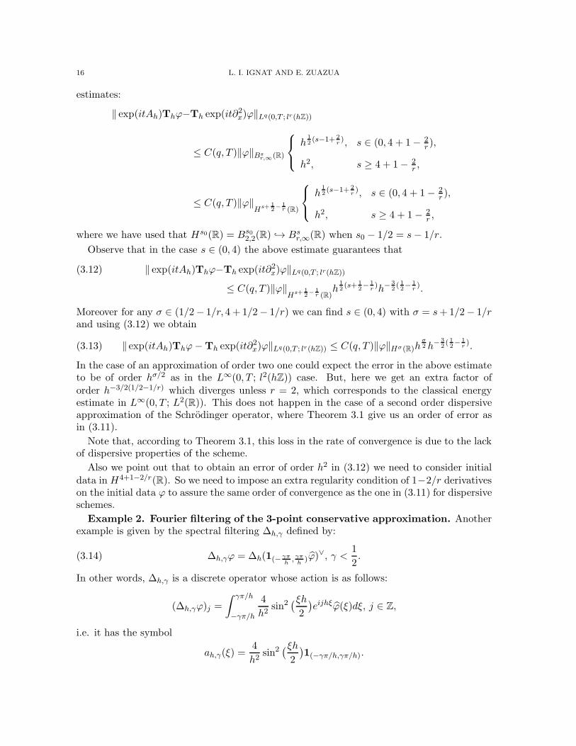
Observe that in the case s ∈ (0, 4) the above estimate guarantees that

‖ exp(itAh)Thϕ−Th exp(it∂2x)ϕ‖Lq(0,T ; lr(hZ))(3.12)

≤ C(q, T )‖ϕ‖Hs+1

2−1r (R)

h12(s+ 1

2− 1

r)h−

32( 12− 1

r).

Moreover for any σ ∈ (1/2− 1/r, 4 + 1/2− 1/r) we can find s ∈ (0, 4) with σ = s+1/2− 1/rand using (3.12) we obtain

(3.13) ‖ exp(itAh)Thϕ−Th exp(it∂2x)ϕ‖Lq(0,T ; lr(hZ)) ≤ C(q, T )‖ϕ‖Hσ(R)h

σ2 h−

32( 12− 1

r).

In the case of an approximation of order two one could expect the error in the above estimateto be of order hσ/2 as in the L∞(0, T ; l2(hZ)) case. But, here we get an extra factor of

order h−3/2(1/2−1/r) which diverges unless r = 2, which corresponds to the classical energyestimate in L∞(0, T ; L2(R)). This does not happen in the case of a second order dispersiveapproximation of the Schrodinger operator, where Theorem 3.1 give us an order of error asin (3.11).

Note that, according to Theorem 3.1, this loss in the rate of convergence is due to the lackof dispersive properties of the scheme.

Also we point out that to obtain an error of order h2 in (3.12) we need to consider initial

data in H4+1−2/r(R). So we need to impose an extra regularity condition of 1−2/r derivativeson the initial data ϕ to assure the same order of convergence as the one in (3.11) for dispersiveschemes.

Example 2. Fourier filtering of the 3-point conservative approximation. Anotherexample is given by the spectral filtering ∆h,γ defined by:

(3.14) ∆h,γϕ = ∆h(1(− γπh, γπh)ϕ)

∨, γ <1

2.

In other words, ∆h,γ is a discrete operator whose action is as follows:

(∆h,γϕ)j =

∫ γπ/h

−γπ/h

4

h2sin2

(ξh2

)eijhξϕ(ξ)dξ, j ∈ Z,

i.e. it has the symbol

ah,γ(ξ) =4

h2sin2

(ξh2

)1(−γπ/h,γπ/h).


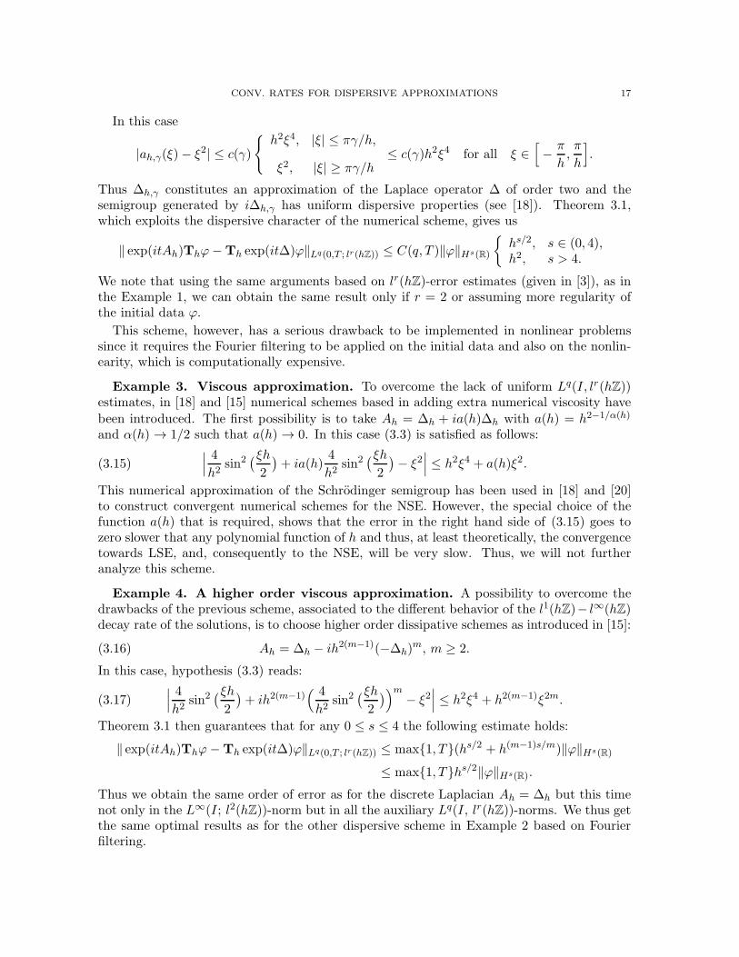
In this case

|ah,γ(ξ)− ξ2| ≤ c(γ)

{h2ξ4, |ξ| ≤ πγ/h,

ξ2, |ξ| ≥ πγ/h≤ c(γ)h2ξ4 for all ξ ∈

[− π

h,π

h

].

Thus ∆h,γ constitutes an approximation of the Laplace operator ∆ of order two and thesemigroup generated by i∆h,γ has uniform dispersive properties (see [18]). Theorem 3.1,which exploits the dispersive character of the numerical scheme, gives us

‖ exp(itAh)Thϕ−Th exp(it∆)ϕ‖Lq(0,T ; lr(hZ)) ≤ C(q, T )‖ϕ‖Hs(R)

{hs/2, s ∈ (0, 4),h2, s > 4.

We note that using the same arguments based on lr(hZ)-error estimates (given in [3]), as inthe Example 1, we can obtain the same result only if r = 2 or assuming more regularity ofthe initial data ϕ.

This scheme, however, has a serious drawback to be implemented in nonlinear problemssince it requires the Fourier filtering to be applied on the initial data and also on the nonlin-earity, which is computationally expensive.

Example 3. Viscous approximation. To overcome the lack of uniform Lq(I, lr(hZ))estimates, in [18] and [15] numerical schemes based in adding extra numerical viscosity have

been introduced. The first possibility is to take Ah = ∆h + ia(h)∆h with a(h) = h2−1/α(h)

and α(h) → 1/2 such that a(h) → 0. In this case (3.3) is satisfied as follows:

(3.15)∣∣∣ 4h2

sin2(ξh2

)+ ia(h)

4

h2sin2

(ξh2

)− ξ2

∣∣∣ ≤ h2ξ4 + a(h)ξ2.

This numerical approximation of the Schrodinger semigroup has been used in [18] and [20]to construct convergent numerical schemes for the NSE. However, the special choice of thefunction a(h) that is required, shows that the error in the right hand side of (3.15) goes tozero slower that any polynomial function of h and thus, at least theoretically, the convergencetowards LSE, and, consequently to the NSE, will be very slow. Thus, we will not furtheranalyze this scheme.

Example 4. A higher order viscous approximation. A possibility to overcome thedrawbacks of the previous scheme, associated to the different behavior of the l1(hZ)− l∞(hZ)decay rate of the solutions, is to choose higher order dissipative schemes as introduced in [15]:

(3.16) Ah = ∆h − ih2(m−1)(−∆h)m, m ≥ 2.

In this case, hypothesis (3.3) reads:

(3.17)∣∣∣ 4h2

sin2(ξh2

)+ ih2(m−1)

( 4

h2sin2

(ξh2

))m− ξ2

∣∣∣ ≤ h2ξ4 + h2(m−1)ξ2m.

Theorem 3.1 then guarantees that for any 0 ≤ s ≤ 4 the following estimate holds:

‖ exp(itAh)Thϕ−Th exp(it∆)ϕ‖Lq(0,T ; lr(hZ)) ≤ max{1, T}(hs/2 + h(m−1)s/m)‖ϕ‖Hs(R)

≤ max{1, T}hs/2‖ϕ‖Hs(R).

Thus we obtain the same order of error as for the discrete Laplacian Ah = ∆h but this timenot only in the L∞(I; l2(hZ))-norm but in all the auxiliary Lq(I, lr(hZ))-norms. We thus getthe same optimal results as for the other dispersive scheme in Example 2 based on Fourierfiltering.


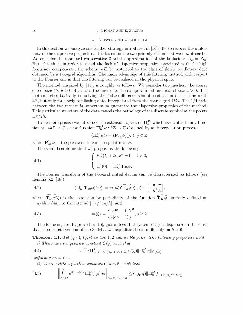
4. A two-grid algorithm

In this section we analyze one further strategy introduced in [16], [18] to recover the unifor-mity of the dispersive properties. It is based on the two-grid algorithm that we now describe.We consider the standard conservative 3-point approximation of the laplacian: Ah = ∆h.But, this time, in order to avoid the lack of dispersive properties associated with the highfrequency components, the scheme will be restricted to the class of slowly oscillatory dataobtained by a two-grid algorithm. The main advantage of this filtering method with respectto the Fourier one is that the filtering can be realized in the physical space.

The method, inspired by [12], is roughly as follows. We consider two meshes: the coarseone of size 4h, h > 0, 4hZ, and the finer one, the computational one, hZ, of size h > 0. Themethod relies basically on solving the finite-difference semi-discretization on the fine meshhZ, but only for slowly oscillating data, interpolated from the coarse grid 4hZ. The 1/4 ratiobetween the two meshes is important to guarantee the dispersive properties of the method.This particular structure of the data cancels the pathology of the discrete symbol at the points±π/2h.

To be more precise we introduce the extension operator Π4hh which associates to any func-

tion ψ : 4hZ → C a new function Π4hh ψ : hZ → C obtained by an interpolation process:

(Π4hh ψ)j = (P1

4hψ)(jh), j ∈ Z,

where P14hψ is the piecewise linear interpolator of ψ.

The semi-discrete method we propose is the following:

(4.1)

iuht (t) + ∆huh = 0, t > 0,

uh(0) = Π4hh T4hϕ.

The Fourier transform of the two-grid initial datum can be characterized as follows (seeLemma 5.2, [18]):

(4.2) (Π4hh T4hϕ)

∧(ξ) = m(hξ)T4hϕ(ξ), ξ ∈[−πh,π

h

],

where T4hϕ(ξ) is the extension by periodicity of the function T4hϕ, initially defined on[−π/4h, π/4h], to the interval [−π/h, π/h], and

(4.3) m(ξ) =

(e4iξ − 1

4(eiξ − 1)

)2

, p ≥ 2.

The following result, proved in [16], guarantees that system (4.1) is dispersive in the sensethat the discrete version of the Strichartz inequalities hold, uniformly on h > 0.

Theorem 4.1. Let (q, r), (q, r) be two 1/2-admissible pairs. The following properties hold

i) There exists a positive constant C(q) such that

(4.4) ‖eit∆hΠ4hh ϕ‖Lq(R, lr(hZ)) ≤ C(q)‖Π4h

h ϕ‖l2(hZ)uniformly on h > 0.

ii) There exists a positive constant C(d, r, r) such that

(4.5)

∥∥∥∥∫

s<tei(t−s)∆hΠ4h

h f(s)ds

∥∥∥∥Lq(R, lr(hZ))

≤ C(q, q)‖Π4hh f‖Lq′(R, lr′(hZ))


for all f ∈ Lq′(R, lr′

(4hZ)), uniformly in h > 0.

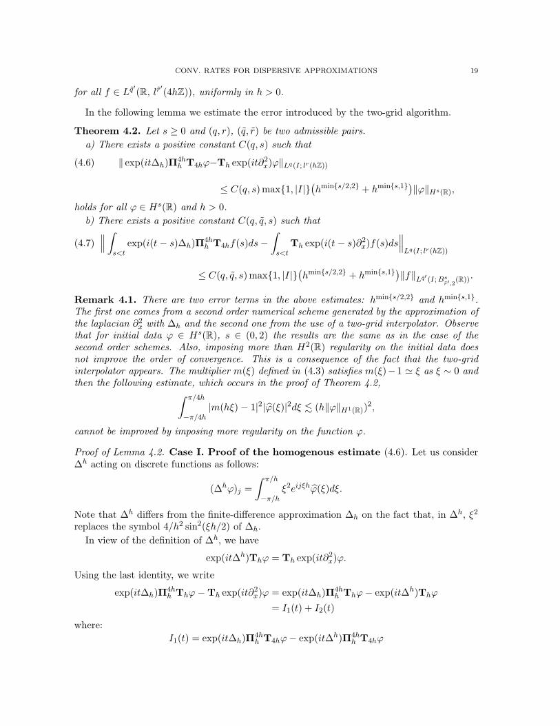
In the following lemma we estimate the error introduced by the two-grid algorithm.

Theorem 4.2. Let s ≥ 0 and (q, r), (q, r) be two admissible pairs.

a) There exists a positive constant C(q, s) such that

‖ exp(it∆h)Π4hh T4hϕ−Th exp(it∂

2x)ϕ‖Lq(I; lr(hZ))(4.6)

≤ C(q, s)max{1, |I|}(hmin{s/2,2} + hmin{s,1})‖ϕ‖Hs(R),

holds for all ϕ ∈ Hs(R) and h > 0.

b) There exists a positive constant C(q, q, s) such that∥∥∥∫

s<texp(i(t− s)∆h)Π

4hh T4hf(s)ds−

∫

s<tTh exp(i(t− s)∂2x)f(s)ds

∥∥∥Lq(I; lr(hZ))

(4.7)

≤ C(q, q, s)max{1, |I|}(hmin{s/2,2} + hmin{s,1})‖f‖Lq′ (I;Bs

r′,2(R)).

Remark 4.1. There are two error terms in the above estimates: hmin{s/2,2} and hmin{s,1}.The first one comes from a second order numerical scheme generated by the approximation ofthe laplacian ∂2x with ∆h and the second one from the use of a two-grid interpolator. Observethat for initial data ϕ ∈ Hs(R), s ∈ (0, 2) the results are the same as in the case of thesecond order schemes. Also, imposing more than H2(R) regularity on the initial data doesnot improve the order of convergence. This is a consequence of the fact that the two-gridinterpolator appears. The multiplier m(ξ) defined in (4.3) satisfies m(ξ)−1 ≃ ξ as ξ ∼ 0 andthen the following estimate, which occurs in the proof of Theorem 4.2,

∫ π/4h

−π/4h|m(hξ)− 1|2|ϕ(ξ)|2dξ . (h‖ϕ‖H1(R))

2,

cannot be improved by imposing more regularity on the function ϕ.

Proof of Lemma 4.2. Case I. Proof of the homogenous estimate (4.6). Let us consider∆h acting on discrete functions as follows:

(∆hϕ)j =

∫ π/h

−π/hξ2eijξhϕ(ξ)dξ.

Note that ∆h differs from the finite-difference approximation ∆h on the fact that, in ∆h, ξ2

replaces the symbol 4/h2 sin2(ξh/2) of ∆h.

In view of the definition of ∆h, we have

exp(it∆h)Thϕ = Th exp(it∂2x)ϕ.

Using the last identity, we write

exp(it∆h)Π4hh Thϕ−Th exp(it∂

2x)ϕ = exp(it∆h)Π

4hh Thϕ− exp(it∆h)Thϕ

= I1(t) + I2(t)

where:

I1(t) = exp(it∆h)Π4hh T4hϕ− exp(it∆h)Π4h

h T4hϕ


and

I2(t) = exp(it∆h)Π4hh T4hϕ− exp(it∆h)Thϕ.

In the following we estimate each of them.

Applying Theorem 2.2 to operators ∆h and ∆h we get

‖I1‖Lq(0,T ; lr(hZ)) ≤ hmin{s/2,2} max{1, T}‖Π4hh T4hϕ‖Bs

2,2(hZ)≤ hmin{s/2,2} max{1, T}‖ϕ‖Hs(R).

In the case of I2 we claim that for any s ≥ 0

(4.8) ‖I2‖Lq(0,T ; lr(hZ)) ≤ hmin{s,1}‖ϕ‖Hs(R).

To prove this claim, we remark that the operator exp(it∆h) satisfies (2.1) and (2.2). ThusProposition 2.1 guarantees that exp(it∆h) has uniform Strichartz estimates and

(4.9) ‖I2‖Lq(0,T ; lr(hZ)) ≤ ‖Π4hh T4hϕ−Thϕ‖l2(hZ).

It is then sufficient to prove that

(4.10) ‖Π4hh T4hϕ−Thϕ‖l2(hZ) ≤ hmin{s,1}‖ϕ‖Hs(R)

holds for any s ≥ 0. Actually it suffices to prove it for 0 ≤ s ≤ 1. Also the cases s ∈ (0, 1)follow by intepolation between the cases s = 0 and s = 1. We will consider now these twocases.

The case s = 0 easily follows since

‖|Π4hh T4hϕ‖l2(hZ) . ‖T4hϕ‖l2(4hZ) . ‖ϕ‖L2(R)

and

‖Thϕ‖l2(hZ) . ‖ϕ‖L2(R).

We now prove (4.10) in the case s = 1:

(4.11) ‖Π4hh T4hϕ−Thϕ‖l2(hZ) . h‖ϕ‖H1(R).

Using that

‖T4hϕ−Thϕ‖l2(hZ) ≤(∫

|ξ|≥π/4h|ϕ(ξ)|2dξ

)1/2. h‖ϕ‖H1(R),

it is sufficient to prove the following estimate

(4.12) ‖Π4hh T4hϕ−T4hϕ‖l2(hZ) . h‖ϕ‖H1(R).

The representation formula (4.2) gives us that

‖Π4hh T4hϕ−T4hϕ‖2l2(hZ) ≤

∫ π/4h

−π/4h|m(hξ)− 1|2|ϕ(ξ)|2dξ(4.13)

+

∫

π/4h≤|ξ|≤π/h|m(hξ)|2|T4hϕ(ξ)|2dξ.

Using that |m(ξ)− 1| ≤ |ξ| for ξ ∈ [−π/4, π/4] we obtain

(4.14)

∫ π/4h

−π/4h|m(hξ)− 1|2|ϕ(ξ)|2dξ . (h‖ϕ‖H1(R))

2.


Previous results on the Fourier analysis of the two-grid method (see [19], Appendix B) and

the periodicity with period π/2h of the function T4hϕ(ξ) give us that∫

π/4h≤|ξ|≤π/h|m(hξ)|2|T4hϕ(ξ)|2dξ =

∫

π/4h≤|ξ|≤π/h

∣∣∣∣e4iξh − 1

4(eiξh − 1)

∣∣∣∣4

|T4hϕ(ξ)|2

.

∫

π/4h≤|ξ|≤π/h|e4iξh − 1|4|T4hϕ(ξ))|2 .

∫

−π/4h≤ξ≤π/4h|e4iξh − 1|4|T4hϕ(ξ)|2

.

∫

−π/4h≤ξ≤π/4h|ξh|4|T4hϕ(ξ)|2dξ . (h‖ϕ‖H1(R))

2.

We obtain that (4.12) holds and, consequently, (4.11) too. Thus (4.8) is satisfied for anypositive s.

Observe that the main term in the right hand side of (4.13) is given by (4.14), and thisestimate cannot be improved by imposing more than H1(R) smoothness on ϕ.

Case II. Proof of the inhomogeneous estimate (4.7). We proceed as in the previouscase by splitting the difference we want to evaluate as∫

s<texp(i(t− s)∆h)Π

4hh T4hf(s)ds−

∫

s<tTh exp(i(t− s)∂2x)f(s)ds = I1 + I2

where

I1 =

∫

s<t

(exp(i(t− s)∆h)− exp(i(t − s)∆h)

)Π4h

h T4hf(s)ds,

and

I2 =

∫

s<texp(i(t − s)∆h)(Π4h

h T4hf(s)−Thf(s))ds.

In the case of I1, applying Theorem 2.2 to operators ∆h and ∆h, we get

‖I1‖Lq(0,T ;lr(hZ)) ≤ hmin{s/2,2} max{1, T}‖Π4hh T4hf‖Lq′ (0,T ;Bs

r′,2(hZ)).

Applying Theorem 7.1 below to the multiplier m given by (4.3), for any s > 0 we obtain that

‖Π4hh T4hf‖Lq′(0,T ;Bs

r′,2(hZ)) ≤ ‖f‖Lq′ (0,T ;Bs

r′,2(R))

and then I1 satisfies:

(4.15) ‖I1‖Lq(0,T ;lr(hZ)) ≤ hmin{s/2,2} max{1, T}‖f‖Lq′ (0,T ;Bsr′,2

(R)).

In the case of I2 we claim that

(4.16) ‖I2‖Lq(0,T ;lr(hZ)) ≤ hmin{s,1}‖f‖Lq′ (0,T ;Bsr′,2

(R)).

To prove this claim we consider the cases s = 0 and s = 1. When s ∈ (0, 1) we use interpolationbetween the previous ones. Also the case s > 1 follows by using the embedding Bs

r′,2(R) →B1

r′,2(R).

The case s = 0 follows from Proposition 2.1 applied to the operators Uh(t) = Th exp(it∂2x).

We now consider the case s = 1. Using Strichartz estimates given by Proposition 2.1 tothe operator exp(it∆h) we get:

‖I2‖Lq(0,T ;lr(hZ)) ≤ ‖Π4hh T4hf −Thf‖Lq′ (0,T ; lr′(hZ)).


Theorem 7.1 applied to the multiplier m gives us

‖Π4hh T4hf −T4hf‖Lq′(0,T ; lr′(hZ)) ≤ h‖f‖Lq′ (0,T ;B1

r′,2(R))

and‖T4hf −Thf‖Lq′(0,T ; lr′(hZ)) ≤ h‖f‖Lq′ (0,T ;B1

r′,2(R)).

Thus (4.16) holds for s = 1, and in view of the above comments, for all s ≥ 0.

Putting together (4.15) and (4.15) we obtain the inhomogeneous estimate (4.7).

The proof is now complete. �

5. Convergence of the dispersive method for the NSE

In this section we introduce numerical schemes for the NSE based on dispersive approxi-mations of the LSE. We first present some classical results on well-posedness and regularityof solutions of the NSE. Secondly we obtain the order of convergence for the approximationsof the NSE described above.

5.1. Classical facts on NSE. We consider the NSE with nonlinearity f(u) = |u|pu andϕ ∈ Hs(R). We are interested in the case of Hs(R) initial data with s ≤ 1. The followingwell-posedness result is known.

Theorem 5.1. Let f(u) = |u|pu with p ∈ (0, 4). Then

i) (Global existence and uniqueness, [5], Th. 4.6.1, Ch. 4, p. 109)For any ϕ ∈ L2(R), there exists a unique global solution u of (1.2) in the class

u ∈ C(R, L2(R)) ∩ Lqloc(R, L

r(R))

for all 1/2-admissible pairs (q, r) such that

‖u(t)‖L2(R) = ‖ϕ‖L2(R), ∀ t ∈ R.

ii) (Stability, [5], Th. 4.6.1, Ch. 4, p. 109) Let ϕ and ψ be two L2(R) functions, and u andv the corresponding solutions of the NSE. Then for any T > 0 there exists a positive constantC(T, ‖ϕ‖L2(R), ‖ψ‖L2(R)) such that the following holds

(5.1) ‖u− v‖L∞(0,T ;L2(R)) ≤ C(T, ‖ϕ‖L2(R), ‖ψ‖L2(R))‖ϕ − ψ‖L2(R)

iii) (Regularity) Moreover if ϕ ∈ Hs(R), s ∈ (0, 1/2) then ([5], Theorem 5.1.1, Ch. 5,p. 147)

u ∈ C(R,Hs(R)) ∩ Lqloc(R, B

sr,2(R))

for every admissible pairs (q, r).

Also if ϕ ∈ H1(R) then u ∈ C(R,H1(R)) ([5], Theorem 5.2.1, Ch. 5, p. 149).

Remark 5.1. The embedding Bsr,2(R) → W s,r(R), r ≥ 2, (see [5], Remark 1.4.3, p. 14)

guarantees that, in particular, u ∈ Lqloc(R,W

s,r(R)). Moreover, f(u) ∈ Lq′

loc(R, Bsr′,2(R)) and

for any 0 < s ≤ 1 (see [5], formula (4.9.20), p. 128)

(5.2) ‖f(u)‖Lq′ (I,Bsr′,2

(R)) . |I|4−p(1−2s)

4 ‖u‖p+1Lq(I,Bs

r,2(R)).

The fixed point argument used to prove the existence and uniqueness result in Theorem5.1 gives us also quantitative information of the solutions of NSE in terms of the L2(R)-normof the initial data. The following holds:


Lemma 5.1. Let ϕ ∈ L2(R) and u be the solution of the NSE with initial data ϕ andnonlinearity f(u) = |u|pu, p ∈ (0, 4), as in Theorem 5.1. There exists c(p) > 0 and T0 =

c(p)‖ϕ‖−4p/(4−p)L2(R)

such that for any 1/2-admissible pairs (q, r), there exists a positive constant

C(p, q) such that

(5.3) ‖u‖Lq(I;Lr(R)) ≤ C(p, q)‖ϕ‖L2(R)

holds for all intervals I with |I| ≤ T0.

Proof of Lemma 5.1. Let us fix an admissible pair (q, r). The fixed point argument used inthe proof of Theorem 5.1 (see ([4], Th. 5.5.1, p. 15) gives us the existence of a time T0,

T0 = c(p)‖ϕ‖−4p4−p

L2(R),

such that

‖u‖Lq(0,T0;Lr(R)) ≤ C(p, q)‖ϕ‖L2(R).

The same argument applied to the interval [(k − 1)T0, kT0], k ≥ 1, and the conservation ofthe L2(R)-norm of the solution u of the NSE gives us that

‖u‖Lq((k−1)T0, kT0;Lr(R)) ≤ C(p, q)‖u((k − 1)T0)‖L2(R) = C(p, q)‖ϕ‖L2(R).

This proves (5.3) and finishes the proof of Lemma 5.1. �

5.2. Approximation of the NSE by dispersive numerical schemes. In this sectionwe consider a numerical scheme for the NSE based on approximations of the LSE that hasuniform dispersive properties of Strichartz type. Examples of such schemes have been givenin Section 3 and Section 4.

To be more precise, we deal with the following numerical schemes:

• Consider

(5.4)

{iuht +Ahu

h = f(uh), t > 0,

uh(0) = ϕh,

where Ah is an approximation of ∆ such that exp(itAh) has uniform dispersive prop-erties of Strichartz type. We also assume that Ah satisfies Re(iAhϕ,ϕ)h ≤ 0, ℜ beingthe real part, and has a symbol ah(ξ) which verifies

(5.5) |ah(ξ)− ξ2| ≤∑

k∈Fa(k, h)|ξ|k, ξ ∈

[−πh,π

h

].

• The two-grid scheme. The two-grid scheme can be adapted to the nonlinear frame asfollows. Consider the equation

(5.6)

iu0,ht +∆hu0,h = Π4h

h f((Π4hh )∗u0,h), t > 0,

u0,h(0) = Π4hh ϕ

h,

where (Π4hh )∗ : l2(hZ) → l2(4hZ) is the adjoint of Π4h

h : l2(4hZ) → l2(hZ) and ϕh isan approximation of ϕ.


By [16], Theorem 4.1, for any p ∈ (0, 4) there exists of a positive time T0 =T0(‖ϕ‖L2(R)) and a unique solution uh,0 ∈ C(0, T0; l

2(hZd)) ∩ Lq(0, T0; lp+2(hZd)),

q = 4(p + 2)/p, of the system (5.6). Moreover, uh,0 satisfies

(5.7) ‖uh‖L∞(R, l2(hZd)) ≤ ‖Π4hh ϕ

h‖l2(hZd)

and

(5.8) ‖uh‖Lq(0,T0; lp+2(hZd)) ≤ c(T0)‖Π4hh ϕ

h‖l2(hZd),

where the above constant is independent of h.With T0 obtained above, for any k ≥ 1 we consider uk,h : [kT0, (k + 1)T0] → C the

solution of the following system

(5.9)

iuk,ht +∆huk,h = Π4h

h f((Π4hh )∗uk,h), t ∈ [kT0, (k + 1)T0],

uk,h(kT0) = Π4hh u

k−1,h(kT0).

Once, uk,h are computed the approximation uh of NSE is defined as

(5.10) uh(t) = uk,h(t), t ∈ [kT0, (k + 1)T0).

We point out that systems (5.6) and (5.9) have always a global solution in the classC(R, l2(hZ)) (use the embedding l2(hZ) ⊂ l∞(hZ), a classical fix point argument andthe conservation of the l2(hZ)-norm). However, estimates in the Lq(0, T ; lr(hZ))-norm, uniformly with respect to the mesh-size parameter h > 0, cannot be provedwithout using Strichartz estimates given by Theorem 4.1. Thus we need to takeinitial data obtained through a two-grid process. Since the two-grid class of functionsis not invariant under the flow of system (5.6) we need to update the solution at sometime-step T0 which depends only on L2(R)-norm of the initial data ϕ.

The following theorems give us the existence and uniqueness of solutions for the abovesystems as well as quantitative dispersive estimates of solutions uh, similar to those obtainedin Lemma 5.1 for the continuous NSE, uniformly on the mesh-size parameter h > 0.

Theorem 5.2. Let p ∈ (0, 4), f(u) = |u|pu and Ah be such that Re(iAhϕ,ϕ)h ≤ 0 and (3.5)holds. Then for every ϕh ∈ l2(hZ), there exists a unique global solution uh ∈ C(R, l2(hZ)) of(5.4) which satisfies

(5.11) ‖uh‖L∞(R, l2(hZ)) ≤ ‖ϕh‖l2(hZ).Moreover, there exist c(p) > 0 and C(p, q) > 0 such that for any finite interval I with

|I| ≤ T0 = c(p)‖ϕh‖−4p/(4−p)l2(hZ)

(5.12) ‖uh‖Lq(I, lr(hZ)) ≤ C(p, q)‖ϕh‖l2(hZ),where (q, r) is a 1/2-admissible pair and the above constant is independent of h.

Proof. Condition Re(iAhϕ,ϕ)h ≤ 0 implies the l2(hZ) stability property (3.4). Then localexistence is obtained by using Strichartz estimates given by Proposition 2.1 applied to theoperator exp(itAh) and a classical fix point argument in a suitable Banach space (see [18] and[20] for more details). The global existence of solutions and estimate (5.11) are guaranteedby the property Re(iAhϕ,ϕ)h ≤ 0, and that Re(if(uh), uh)h = 0 and the energy identity:

(5.13)d

dt‖uh(t)‖2l2(hZ) = 2Re(iAhu

h, uh)h + 2Re(if(uh), uh)h ≤ 0.


Once the global existence is proved, estimate (5.12) is obtained in a similar manner as Lemma5.1 and we will omit its proof. �

Theorem 5.3. Let p ∈ (0, 4) and q = 4(p + 2)/p. Then for all h > 0 and for everyϕh ∈ l2(4hZ), there exists a unique global solution uh ∈ C(R, l2(hZ)) ∩ Lq

loc(R, lp+2(hZd)) of

(5.6)-(5.10) which satisfies

(5.14) ‖uh‖L∞(R, l2(hZ)) ≤ ‖Π4hh ϕ

h‖l2(hZ).Moreover, there exist c(p) > 0 and C(p, q) > 0 such that for any finite interval I with

|I| ≤ T0 = c(p)‖ϕh‖−4p/(4−p)l2(hZ)

(5.15) ‖uh‖Lq(I, lp+2(hZ)) ≤ C(p, q)‖Π4hh ϕ

h‖l2(hZ),where (q, r) is a 1/2-admissible pair and the above constant is independent of h.

Proof. The existence in the interval (0, T0), T0 = T0(‖ϕh‖l2(hZ)) for system (5.4) is obtainedby using the Strichartz estimates given by Theorem 4.1 and a classical fix point argument ina suitable Banach space (see [18] and [20] for more details).

For any k ≥ 1 the same arguments guarantee the local existence for systems (5.9). Toprove that each system has solutions on an interval of length T0 we have to prove a priori thatthe l2(hZ)-norm of uh does not increase. The particular approximation we have introducedof the nonlinear term in (5.6)-(5.9) gives us (after multiplying these equations by uk,h andtaking the l2(hZ)-norm) that for any t ∈ [kT0, (k + 1)T0]

‖uk,h(t)‖l2(hZ) = ‖uk,h(kT0)‖l2(hZ) ≤ ‖uk−1,h(kT0)‖l2(hZ)and then

‖uk,h(t)‖l2(hZ) ≤ ‖u0,h(0)‖l2(hZ) = ‖Π4hh ϕ

h‖l2(hZ).This proves (5.14) and the fact that for any k ≥ 1 system (5.9) has a solution on the whole

interval [kT0, (k + 1)T0]. Estimate (5.15) is obtained locally on each interval [kT0, (k + 1)T0]together with the local existence result. �

Let us consider uh the solution of the semidiscrete problem (5.4) and u of the continuousone (1.2). In the following theorem we evaluate the difference between uh and Thu.

Theorem 5.4. Let p ∈ (0, 4), s ∈ (0, 1/2), f(u) = |u|pu and Ah be as in Theorem 5.2 satis-fying (5.5). For any ϕ ∈ Hs(R), we consider uh and u ∈ L∞(R, Hs(R))∩Lq0

loc(R, Bsp+2,2(R)),

q0 = 4(p+2)/p solutions of problems (5.4) and (1.2), respectively. Then for any T > 0 thereexists a positive constant C(T, ‖ϕ‖L2(R)) such that

‖uh −Thu‖Lq0 (0,T ; lp+2(hZ)) + ‖uh −Thu‖L∞(0,T ; l2(hZ))

(5.16)

≤ C(T, ‖ϕ‖L2(R), p)[ε(s, h)‖u‖L∞(0,T ;Hs(R)) +

(hs + ε(s, h)

)‖u‖p+1

Lq0 (0,T ;Bsp+2,2(R))

]

holds for all h > 0.

In the case of the two-grid method, the solution uh of system (5.6) approximates thesolution u of the NSE (1.2) and the error committed is given by the following theorem.


Theorem 5.5. Let p ∈ (0, 4), s ∈ (0, 1/2), f(u) = |u|pu. For any ϕ ∈ Hs(R), we consider uh

and u ∈ L∞(R, Hs(R))∩Lq0loc(R, B

sp+2,2(R)), q0 = 4(p+2)/p, solutions of problems (5.6)-(5.10)

and (1.2), respectively. Then for any T > 0 there exists a positive constant C(T, ‖ϕ‖L2(R))such that

‖uh −Thu‖Lq0 (0,T ; lp+2(hZ)) + ‖uh −Thu‖L∞(0,T ; l2(hZ))(5.17)

≤ C(T, ‖ϕ‖L2(R), p)[hs/2‖u‖L∞(0,T ;Hs(R)) +

(hs + hs/2

)‖u‖p+1

Lq0 (0,T ;Bsp+2,2(R))

]


Remark 5.2. Using classical results on the solutions of the NSE (see for example [4], The-orem 5.1.1, Ch. 5, p. 147) we can state the above result in a more compact way: For anyT > 0 there exists a positive constant C(T, ‖ϕ‖Hs(R)) such that

‖uh −Thu‖Lq0 (0,T ; lp+2(hZ)) + ‖uh −Thu‖L∞(0,T ; l2(hZ)) ≤ C(T, ‖ϕ‖Hs(R))hs/2(5.18)


Theorem 5.4 shows that if hs ≤ ε(s, h) then the error committed to approximate thenonlinear problem is the same as for the linear problem with the same initial data. As weproved in Section 3.2, for the higher order dissipative scheme Ah = ∆h − ih2(m−1)(−∆h)

m,m ≥ 2, and for the two-grid method, ε(s, h) = hs/2 ≥ hs. So these schemes enter in thisframework. It is also remarkable that the use of dispersive schemes allows to prove theconvergence for the NSE and to obtain the convergence rate for Hs(R) initial data with0 < s < 1/2. We point out that the energy method does not provide any error estimate inthis case, the minimal smoothing required for the energy method being Hs(R), with s > 1/2(see Section 6 for all the details).

In the following we prove Theorem 5.4, the proof of Theorem 5.5 being similar sincethe estimates in any interval (0, T ) are obtained reiterating the argument in each interval(kT0, (k + 1)T0), k ≥ 0, for some T0 = T0(‖ϕ‖L2(R)) in view of the structure of the scheme.

Proof of Theorem 5.4. The idea of the proof is that there exists a time T1 depending on theL2(R)-norm of the initial data:

T1 ≃ min{1, ‖ϕ‖−4p/(4−p)L2(R)

},

such that the error in the approximation of the nonlinear problem

errh(t) = uh(t)−Thu(t),

when considered in the Lq0(0, T1; lp+2(hZ))∩L∞(0, T1; l

2(hZ))-norm is controlled by the errorproduced in the linear part

errlinh (t) = exp(itAh)Thϕ−Th exp(it∂2x)ϕ.

In the following we denote by (q, r) one of the admissible pairs (∞, 2) or (q0, p + 2). Wenow write the two solutions in the semigroup formulation given by systems (5.4) and (1.2):

uh(t) = exp(itAh)Thϕ+ i

∫ t

0exp(i(t− s)Ah)f(u

h(s))ds,


and, respectively,

Thu(t) = Th exp(it∂2x)ϕ+ i

∫ t

0Th exp(i(t− s)∂2x)f(u(s))ds.

Thus

(5.19) ‖errh‖Lq(0,T ; lr(hZ)) ≤ ‖errlinh ‖Lq(0,T ; lr(hZ)) + ‖errnonh ‖Lq(0,T ; lr(hZ))

where, by definition,

errnonh (t) =

∫ t

0exp(i(t− s)Ah)f(u

h(s))ds −∫ t

0Th exp(i(t− s)∂2x)f(u(s))ds.

For the linear part the error is estimated in Theorem 3.1:

(5.20) ‖errlinh ‖Lq(0,T ; lr(hZ)) ≤ C(q)ε(s, h)max{T, 1}‖ϕ‖Hs(R).

In the following we will estimate errnonh . We write errnonh (t) = Ih2 (t) + Ih3 (t) where

Ih2 (t) =

∫ t

0exp(i(t− s)Ah)

(f(uh(s))−Thf(u(s))

)ds

and

Ih3 (t) =

∫ t

0

(exp(i(t − s)Ah)Thf(u(s))−Th exp(i(t− s)∂2x)f(u(s))

)ds.

Step I. Estimate of Ih3 . For the last term, the inhomogeneous estimate (3.8) in Theorem3.1 and estimate (5.2) give us that

‖Ih3 (t)‖Lq(0,T ; lr(hZ)) ≤ C(q)ε(s, h)max{1, T}‖f(u)‖Lq′0 (0,T ;Bs

(p+2)′,2(R))

(5.21)

≤ C(q)ε(s, h)max{1, T}T4−p(1−2s)

4 ‖u‖p+1Lq(0,T ;Bs

p+2,2(R)).

Step II. Estimate of Ih2 . We now prove the existence of a time T0 such that for allT < T0, I

h2 satisfies

‖I2(t)‖Lq(0,T ; lr(hZ))(5.22)

≤ C(p)T 1− p4 ‖errh‖Lq0 (0,T ; lp+2(hZ))‖ϕ‖pL2(R)

+ hsT 1− p4 ‖u‖p+1

Lq0 (0,T ;Bsp+2,2(R))

.

The inhomogeneous Strichartz’s estimate (2.5) applied to the operators (exp(itAh))t≥0

shows that

‖Ih2 (t)‖Lq(0,T ; lr(hZ)) ≤ C(q)‖f(uh)−Thf(u)‖Lq′0 (0,T ; l(p+2)′(hZ))

(5.23)

≤ C(q)‖f(uh)− f(Thu)‖Lq′0 (0,T ; l(p+2)′ (hZ))

+ C(q)‖f(Thu)−Thf(u)‖Lq′0 (0,T ; l(p+2)′ (hZ))

.

We evaluate each term in the right hand side of (2.31). In the case of the first one, applyingHolder’s inequality in time we get

‖f(uh)− f(Thu)‖Lq′0 (0,T ; l(p+2)′ (hZ))

≤ T 1− p4 ‖uh −Thu‖Lq0 (0,T ; lp+2(hZ))

(‖uh‖p

Lq0 (0,T ; lp+2(hZ))+ ‖Thu‖pLq0 (0,T ; lp+2(hZ))

).


Let us now set T0 as it is given by Lemma 5.1 and Theorem 5.2:

T0 ≃ ‖ϕ‖−4p4−p

L2(R).

Thus, by Theorem 5.1, Lemma 5.1 and Theorem 5.3 both uh andThu have their Lq(0, T ; lr(hZ))-norm controlled by the L2-norm of the initial data:

‖uh‖Lq0 (0,T0; lp+2(hZ)) ≤ C(p)‖ϕ‖L2(R)

and

‖Thu‖Lq0 (0,T0; lp+2(hZ)) ≤ C(p)‖u‖Lq0 (0,T0;Lp+2(R)) ≤ C(p)‖ϕ‖L2(R).

These estimates show that for any T < T0 the following holds:

‖f(uh)− f(Thu)‖Lq′0 (0,T ; l(p+2)′(hZ))

≤ C(p)T 1− p4 ‖uh −Thu‖Lq0 (0,T ; lp+2(hZ))‖ϕ‖pL2(R)

.(5.24)

It remains to estimate the second term in the right hand side of (5.23). We will use nowthe following result which will be proved in Section 7.

Lemma 5.2. Let s ∈ [0, 1], p ≥ 0 and f(u) = |u|pu. Then there exists a positive constantc(p, s) such that

(5.25) ‖f(Thu)−Thf(u)‖l(p+2)′(hZ) ≤ c(p, s)hs‖u‖p+1W s,p+2(R)

holds for all u ∈W s,p+2(R) and h > 0.

Using this lemma, Holder inequality in time and the embedding Bsp+2,2(R) → W s,p+2(R)

([5], Remark 1.4.3) we obtain:

‖f(Thu)−Thf(u)‖Lq′0 (0,T ; l(p+2)′(hZ))≤ c(p, s)hsT 1− p

4 ‖u‖p+1Lq0 (0,T ;W s,p+2(R))

(5.26)

≤ c(p, s)hsT 1− p4 ‖u‖p+1

Lq0 (0,T ;Bsp+2,2(R))

.

Both (5.24) and (5.26) show that I2(t) satisfies (5.22).

Step III. Estimate of errh. Collecting estimates (5.20), (5.21) and (5.22) for both(q, r) = (q0, p+ 2) and (q, r) = (∞, 2) we obtain that for any T < T0 the error errh satisfies:

‖errh‖Lq0 (0,T ; lp+2(hZ)) + ‖errh‖L∞(0,T ; l2(hZ))(5.27)

≤C(p)max{1, T}ε(s, h)‖ϕ‖Hs (R) + C(p)‖errh‖Lq0 (0,T ; lp+2(hZ))T1−p/4‖ϕ‖p

L2(R)

+ hsT 1− p4 ‖u‖p+1

Lq0 (0,T ;Bsp+2,2(R))

+ ε(s, h)max{1, T}T4−p(1−2s)

4 ‖u‖p+1Lq0 (0,T ;Bs

p+2,2(R)).

Now, let us set T1 ≤ min{1, T0} such that

C(p)T1−p/41 ‖ϕ‖p

L2(R)≤ 1

2.

Then the error term errh in the right hand side of (5.27) is absorbed in the left hand side:

‖errh‖Lq0 (0,T1; lp+2(hZ)) + ‖errh‖L∞(0,T1; l2(hZ))

≤ C(p)ε(s, h)‖ϕ‖Hs(R) + C(p)‖u‖p+1Lq0 (0,T ;Bs

p+2,2(R))

(hs + ε(s, h)

).


We now obtain the same estimate in any interval (0, T ). Using that the L2(R)-norm of thesolution u is conserved in time we can apply the same argument in the interval [kT1, (k+1)T1]:

‖errh‖Lq0 (kT1,(k+1)T1; lp+2(hZ)) + ‖errh‖L∞(kT1,(k+1)T1; l2(hZ))

≤ C(p)ε(s, h)‖u(kT1)‖Hs(R) + C(p)(hs + ε(s, h)

)‖u‖p+1

Lq0 (kT1,(k+1)T1;Bsp+2,2(R))

.

Let us choose T > 0 and N ≥ 1 an integer such that (N − 1)T1 ≤ T < NT1. Thus

‖errh‖Lq0 (0,T ; lp+2(hZ)) + ‖errh‖L∞(0,T ; l2(hZ))

≤N−1∑

k=0

(‖errh‖Lq0 (kT1,(k+1)T1; lp+2(hZ)) + ‖errh‖L∞(kT1,(k+1)T1; l2(hZ))

)

≤ C(p)ε(s, h)N−1∑

k=0

‖u(kT1)‖Hs(R) + C(p)(hs + ε(s, h)

)N−1∑

k=0

‖u‖p+1Lq0 (kT1,(k+1)T1;Bs

p+2,2(R)).

Using that (p+ 1)/q0 < 1 we have by the discrete Holder’s inequality that

N−1∑

k=0

‖u‖p+1Lq0 (kT1,(k+1)T1;Bs

p+2,2(R))≤ N

1− p+1q0 ‖u‖p+1

Lq0 (0,T ;Bsp+2,2(R))

.

Thus the error satisfies:

‖errh‖Lq0 (0,T ; lp+2(hZ)) + ‖errh‖L∞(0,T ; l2(hZ))

≤ Nε(s, h)‖u‖L∞(0,T ;Hs(R)) +(hs + ε(s, h)

)N

1− p+1q0 ‖u‖p+1

Lq0 (0,T ;Bsp+2,2(R))

≤ N[ε(s, h)‖u‖L∞(0,T ;Hs(R)) +

(hs + ε(s, h)

)‖u‖p+1

Lq0 (0,T ;Bsp+2,2(R))

]

≤ C(T, ‖ϕ‖L2(R))[ε(s, h)‖u‖L∞(0,T ;Hs(R)) +

(hs + ε(s, h)

)‖u‖p+1

Lq0 (0,T ;Bsp+2,2(R))

].

This finishes the proof of Theorem 5.4. �

6. Nondispersive methods

In this section we will consider a numerical scheme for which the operator Ah has no uniform(with respect to the mesh size h) dispersive properties of Strichartz type. Accordingly we maynot use Lq

tLrx estimates for the linear semigroup exp(itAh) and all the possible convergence

estimates need to be based on the fact that the solution u of the continuous problem isuniformly bounded in space and time: u ∈ L∞((0, T );L∞(R)). Thus, the only estimateswe can use are those that the L2-theory may yield. When working with Hs(R)-data withs > 1/2, using L∞(R;Hs(R)) estimates on solutions and Sobolev’s embedding we can getL2-estimates.

There is a classical argument that works whenever the nonlinearity f satisfies

(6.1) |f(u)− f(v)| ≤ C(|u|p + |v|p)|u− v|.Standard error estimates (see Theorem 3.1 with the particular case (q, r) = (∞, 2) or [30],Theorem 10.1.2, p. 201) and Gronwall’s inequality yield when 0 ≤ t ≤ T :

‖uh(t)−Thu(t)‖l2(hZ)(6.2)

≤ h1/2C(T )(‖ϕ‖H1(R) + ‖u‖p+1

L∞(0,T :H1(R))

)exp(T‖u‖p

L∞(0,T ;H1(R))),


for the conservative semi-discrete finite-difference scheme. For the sake of completness we willprove this estimate in Section 6.1.

We emphasize that in order to obtain estimate (6.2) we need to use that the solution u,which we want to approximate, belongs to the space L∞(R), condition which is guaranteedby assuming that the initial data is smooth enough. However, obviously, in general, solutionsof the NSE do not belong to L∞(R) and therefore these estimates can not be applied. Onecan overcome this drawback assuming that the initial data belong to H1(R) or even to Hs(R)with s > 1/2 since in this case Hs(R) → L∞(R). Using H1-energy estimates and Sobolev’sembedding we can deduce L∞-bounds on solutions allowing to apply (6.2). We emphasizethat this standard approach fails to provide any error estimate for initial data in Hs(R) withs < 1/2.

However, this type of error estimate can also be used for Hs(R)-initial data with s < 1/2(or even for L2(R)-initial data), by a density argument. Indeed, given ϕ ∈ Hs(R) with0 ≤ s < 1/2, for any δ > 0 we may choose ϕδ ∈ H1(R) such that

‖ϕ− ϕδ‖Hs(R) ≤ δ.

Let uδ be the solution of NSE corresponding to ϕδ. Obviously, ϕδ being H1(R)-smooth,we can apply standard results as (6.2) to uδ. On the other hand, stability results for NSEallow us to prove the proximity of u and uδ in H

s(R). This allows showing the convergence ofnumerical approximations of uδ, that we may denote by uδ,h, towards the solution u associatedto ϕ as both δ → 0 and h → 0. But for this to be true h needs to be exponentially smallof the order of exp(−1/δ) which is much smaller than the typical mesh-size needed to applythe results of the previous sections on dispersive schemes that required h to be of the orderof δ2/s.

6.1. A classical argument for smooth initial data. In this section we present the tech-nical details of the error estimates in the case of H1(R)-initial data. In this case we donot require the numerical scheme to be dispersive, the only ingredient being the Sobolev’sembedding H1(R) → L∞(R).

Theorem 6.1. Let f(u) = |u|pu with p ∈ (0, 4) and u ∈ C(R, H1(R)) be solution of (1.2)with initial data ϕ ∈ H1(R). Also assume that Ah is an approximation of order two of thelaplace operator ∂2x and uh is the solution of the following system

(6.3)

{iuht +Ahu

h = f(uh), t > 0,

uh(0) = Thϕ,

satisfying ‖uh‖L∞((0,T )×hZ) ≤ C(T, ‖ϕ‖H1(R)).

Then for all T > 0 and h > 0(6.4)

‖uh(t)−Thu(t)‖l2(hZ) ≤ h1/2 max{T, T 2}(‖ϕ‖H1(R)+‖u‖p+1

L∞(0,T :H1(R))

)exp(T‖u‖p

L∞(0,T ;H1(R))).

We now give an example where the hypotheses of the above theorem are verified. Weconsider the following NSE:

(6.5)

{iut + ∂2xu = |u|pu, x ∈ R, t > 0,u(0, x) = ϕ(x), x ∈ R,


and its numerical approximation

(6.6)

{iuht +∆hu

h = |uh|puh, t > 0,

uh(0) = ϕh.

In the case of the continuous problem we have the following conservation laws (see [5], Corol-lary 4.3.4, p. 93):

‖u(t)‖L2(R) = ‖ϕ‖L2(R)

andd

dt

(12

∫

R

|ux(t, x)|2dx+1

p+ 2

∫

R

|u(t, x)|p+2dx)= 0.

The same identities apply in the semi-discrete case (it suffices to multiply the equation (6.6)by uh, respectively uht , to sum over the integers and to take the real part of the resultingidentity):

‖uh(t)‖l2(hZ) = ‖ϕh‖l2(hZ)and

d

dt

(h2

∑

j∈Z

∣∣uhj+1(t)− uhj (t)

h

∣∣2 + h

p+ 2

∑

j∈Z|uhj (t)|p+2

)= 0.

In view of the above identities, the hypotheses of Theorem 6.1 are verified.

Proof of Theorem 6.1. Using the variations of constants formula we get

Thu(t) = Th exp(it∂2x)ϕ+

∫ t

0Th exp(i(t− σ)∂2x)f(u(σ))dσ

and

uh(t) = exp(itAh)Thϕ+

∫ t

0exp(i(t− σ)Ah)f(u

h(σ))dσ.

Then

errh(t) := ‖uh(t)−Thu(t)‖l2(hZ)(6.7)

≤ ‖ exp(itAh)Thϕ−Th exp(it∂2x)ϕ‖l2(hZ)

+

∫ t

0‖ exp(i(t− σ)Ah)

(f(uh(σ)) −Thf(u(σ))

)dσ‖l2(hZ)dσ

+

∫ t

0‖ exp(i(t− σ)Ah)Thf(u(σ))−Th exp((t− σ)∂2x)f(u(σ))‖l2(hZ)dσ.

Now, applying the error estimates for the linear terms as in (3.9) with ε(1, h) = h1/2, we get

(6.8) ‖ exp(itAh))Thϕ−Th exp(it∂2x)ϕ‖l2(hZ) ≤ Th1/2‖ϕ‖H1(R).

Also, using that f(u) = |u|pu we have that ‖f(u)‖H1(R) ≤ C‖u‖pH1(R)

and then by (3.9) we

get∫ t

0‖ exp(i(t− σ)Ah)Thf(u(σ))−Th exp(i(t− σ)∂2x)f(u(σ))‖l2(hZ)dσ(6.9)

≤ CTh1/2‖f(u)‖L1(0,T ;H1(R))

≤ CT 2h1/2‖u‖p+1L∞(0,T ;H1(R))

.


Using the l2(hZ)-stability of exp(itAh), (6.7), (6.8) and (6.9) we obtain

errh(t) ≤ Th1/2‖ϕ‖H1(R) + CT 2h1/2‖u‖p+1L∞(0,T ;H1(R))

+

∫ t

0‖f(uh(σ)) −Thf(u(σ)‖l2(hZ)).

Now we write f(uh(s))−Thf(u(s)) = Ih1 (s) + Ih2 (s) where

Ih1 (s) = f(uh(s))− f(Thu(s)), Ih2 (s) = f(Thu(s))−Thf(u(s)).

In the case of Ih1 we use that f satisfies (6.1) to get

‖Ih1 (s)‖l2(hZ) ≤ C(‖uh(s)‖pl∞(hZ) + ‖Thu(s)‖pl∞(hZ)

)‖uh(s)−Thu(s)‖l2(hZ)

≤ C(‖uh‖pL∞((0,T )×hZ) + ‖u‖pL∞((0,T )×R))‖uh(s)−Thu(s)‖l2(hZ)

≤ C‖u‖pL∞(0,T ;H1(R))

errh(s).

Using the same arguments as in Lemma 5.2 we obtain that

‖Ih2 (s)‖l2(hZ) ≤ h‖u(s)‖p+1H1(R)

.

Putting together all the above estimates, for any 0 ≤ t ≤ T we obtain:

errh(t) ≤ h1/2T‖ϕ‖H1(R) + ‖u‖pL∞(0,T ;H1(R))

∫ t

0errh(σ)dσ

+ hT‖u‖p+1L∞(0,T ;H1(R))

+ T 2h1/2‖u‖p+1L∞(0,T :H1(R))

≤ h1/2 max{T, T 2}(‖ϕ‖H1(R) + ‖u‖p+1

L∞(0,T :H1(R))

)+ ‖u‖p

L∞(0,T ;H1(R))

∫ t

0errh(s)ds.

Applying Gronwall’s Lemma we obtain

errh(t) . h1/2 max{T, T 2}(‖ϕ‖H1(R) + ‖u‖p+1

L∞(0,T :H1(R))

)exp(T‖u‖p

L∞(0,T ;H1(R))).(6.10)

The proof is now finished. �

6.2. Approximating Hs(R), s < 1/2, solutions by smooth ones. Given ϕ ∈ Hs(R) wechoose an approximation ϕ ∈ H1(R) such that ‖ϕ−ϕ‖Hs(R) is small (a similar analysis can bedone by considering ϕδ ∈ Hs1 with s1 > 1/2). For ϕ we consider the following approximationof u solution of the NSE (1.2) with initial data ϕ:

(6.11)

i∂tuh(t) +Ahuh = f(uh), t > 0,

uh(0) = Thϕ,

where the operator Ah is a second order approximation of the Laplace operator. We do notrequire the linear scheme associated to the operator Ah to satisfy uniform dispersive estimates.

Solving (6.11) we obtain an approximation uh of the solutions u of NSE with initial datumϕ, which itself is an approximation of the solution u of the NSE with initial datum ϕ.

In the following Theorem we give an explicit estimate of the distance between uh and u.

Theorem 6.2. Let 0 ≤ s < 1/2, ϕ ∈ Hs(R), and u ∈ C(R; Hs(R)) be the solution of NSEwith initial datum ϕ given by Theorem 5.1. For any T > 0 there exists a positive constantC(T, ‖ϕ‖L2(R)) such that the following holds(6.12)

‖Thu− uh‖L∞(0,T ; l2(hZ)) ≤ C(T, p, ‖ϕ‖L2(R))‖ϕ− ϕ‖L2(R) + h1/2 exp(T‖u‖p

L∞(0,T ;H1(R))

)


for all h > 0 and δ > 0.

In the following we show that the above method of regularizing the initial data ϕ ∈ Hs(R)and then applying the H1(R) theory for that approximation does not give the same rate of

convergence hs/2 obtained in the case of a dispersive method of order two (see (5.18)). Thisoccurs since for ‖ϕ − ϕ‖L2(R) to be small, ‖ϕ‖H1(R) needs to be large and ‖u‖L∞(0,T ;H1(R))

too.

To simplify the presentation we will consider the case p = 2.

Theorem 6.3. Let p = 2, 0 < s < 1/2, ϕ ∈ Hs(R) and u ∈ C(R,Hs(R)) be solution of NSEwith initial data ϕ given by Theorem 5.1 and u∗h be the best approximation with H1(R)-initialdata as given by (6.11) with the conservative approximation Ah = ∆h. Then for any time T ,there exists a constant C(‖ϕ‖Hs(R), T, s) such that

(6.13) ‖Thu− u∗h‖L∞(0,T ; l2(hZ)) ≤ C(‖ϕ‖Hs(R), T, s)| log h|−s

1−s .

To prove this result we will use in an essential manner the following Lemma.

Lemma 6.1. Let 0 < s < 1 and h ∈ (0, 1). Then for any ϕ ∈ Hs(R) the functional Jh,ϕdefined by

(6.14) Jh,ϕ(g) =1

2‖ϕ− g‖2L2(R) +

h

2exp(‖g‖2H1(R))

satisfies:

(6.15) ming∈H1(R)

Jh,ϕ(g) ≤ C(‖ϕ‖Hs(R), s)| log h|−s/(1−s).

Moreover, the above estimate is optimal in the sense that the power of the | log h| term cannotbe improved: for any 0 < ǫ < 1− s there exists ϕǫ ∈ Hs(R) such that

(6.16) lim infh→0

ming∈H1(R) Jh,ϕε(g)

| log h|−(s+ε)/(1−s−ε)> 0.

Remark 6.1. We point out that, to obtain (6.15) and (6.16), we will use in an essentialmanner that s < 1. In fact in the case s = 1 the minimum of Jh over H1(R) is of order h.This can be seen by choosing g = ϕ and observing that Jh(ϕ) = h exp(‖ϕ‖H1(R)). This choice

cannot be done if ϕ ∈ Hs(R)\H1(R).

Proof of Theorem 6.3. Let us choose ϕ ∈ H1(R) which approximates ϕ in Hs(R). Then byTheorem 6.2 we get

‖Thu− uh‖2L∞(0,T ; l2(hZ)) ≤ C(T, ‖ϕ‖L2(R))‖ϕ − ϕ‖2L2(R) + h exp(2T‖ϕ‖2H1(R)

)(6.17)

≤ C(T, ‖ϕ‖L2(R))Jh,√2Tϕ(

√2T ϕ),

where uh is the solution of (6.11) with initial data Thϕ.

For each h fixed, in order to obtain the best approximation u∗h of Thu, we have to choosein the right hand side of the above inequality the function ϕ∗ which minimizes the functionalJh,

√2Tϕ(·) defined by (6.14) over H1(R). Using estimate (6.15) from Lemma 6.1 we obtain


the desired result:

‖Thu− u∗h‖L∞(0,T ; l2(hZ)) ≤ C(‖ϕ‖Hs(R), T, s) minϕ∈H1(R)

Jh,√2Tϕ(

√2T ϕ)

≤ C(‖ϕ‖Hs(R), T, s)| log h|−s

1−s

where u∗h is the solution of (6.11) with initial data Thϕ∗ �

Proof of Lemma 6.1. The functional Jh,ϕ is convex and its minimizer, gh, is unique. Thefunction gh satisfies the following equation:

(6.18) − ϕ+ gh + h exp(‖gh‖2H1(R))(−∆gh + gh) = 0

and so [I + h exp(‖gh‖2H1(R))(I −∆)

]gh = ϕ.

Thus ch = ‖gh‖H1(R) is the unique solution of

(6.19) ch =∥∥∥(I −∆)1/2

[I + h exp(c2h)(I −∆)

]−1ϕ∥∥∥L2(R)

.

Step I. A useful auxiliary function. Let us consider the function qh(x) = hxβ exp(x)−cfor some positive constants β and c. We prove that there exist two constants a1(c) and a2(c)such that the solution xh of the equation qh(x) = 0 satisfies

(6.20) | log h| − β log | log h|+ a1(c) ≤ xh ≤ | log h| − β log | log h|+ a2(c).

Let us choose a real number a. Using that h = exp(−| log h|) we get:

qh((| log h| − β log | log h|+ a)) = (| log h| − β log | log h|+ a)β exp(−β log | log h|+ a)− c

=

(1− β

log | log h|| log h| +

a

| log h|

)β

exp(a)− c

→h→0 exp(a)− c.

Choosing now two constants a1 and a2 such that exp(a1) < c < exp(a2) and using that thefunction qh is increasing we obtain that, for h small enough, xh, solution of qh(x) = 0, satisfies(6.20).

Step II. Upper bounds on ch. Using that ϕ ∈ Hs(R), identity (6.19) gives us

ch =∥∥∥(I −∆)1/2

[I + h exp(c2h)(I −∆)

]−1ϕ∥∥∥L2(R)

=∥∥∥(I −∆)(1−s)/2

[I + h exp(c2h)(I −∆)

]−1(I −∆)s/2ϕ

∥∥∥L2(R)

= (hec2h)(s−1)/2

∥∥∥[hec

2h(I −∆)

](1−s)/2 [I + hec

2h(I −∆)

]−1(I −∆)s/2ϕ

∥∥∥L2(R)

≤ (h exp(c2h))(s−1)/2‖ϕ‖Hs(R),

since, when s ∈ [0, 1], the symbol in the Fourier variable of the operator[hec

2h(I −∆)

](1−s)/2 [I + hec

2h(I −∆)

]−1

is less than one.


Then c2h(h exp(c2h))

1−s ≤ ‖ϕ‖2Hs(R) and

(6.21) (c2h)1/(1−s)hec

2h ≤ ‖ϕ‖2/(1−s)

Hs(R) .

Applying the result of Step I to β = 1/(1− s) and c = ‖ϕ‖2/(1−s)Hs(R) we obtain that ch satisfies:

(6.22) c2h ≤ | log h| − 1

1− slog | log h|+ a2,

for some constant a2 = a2(‖ϕ‖2/(1−s)Hs(R) ). In particular, when s < 1,

h exp(c2h) = exp(c2h − | log h|) ≤ exp(− 1

1− slog | log h|+ a2

)→ 0,

as h→ 0.

Step III. Estimates on Jh(gh). Using that the minimizer gh satisfies equation (6.18)and ch = ‖gh‖H1(R), we get

2 ming∈H1(R)

Jh(g) = 2Jh(gh) = ‖ϕ− gh‖L2(R) + h exp(‖gh‖2H1(R))

= (h exp(c2h))2‖(I −∆)gh‖2L2(R) + h exp(c2h)

= (h exp(c2h))2‖(I −∆)

[I + h exp(c2h)(I −∆)

]−1ϕ‖2L2(R) + h exp(c2h)

= (hec2h)s

∥∥∥[hec

2h(I −∆)

]1−s/2 [I + hec

2h(I −∆)

]−1(I −∆)s/2ϕ

∥∥∥2

L2(R)+ hec

2h

≤ (hec2h)s‖ϕ‖2Hs(R) + hec

2h ≤ (hec

2h)s

(‖ϕ‖2Hs(R) + (hec

2h)1−s

)

≤ c(s, ‖ϕ‖Hs(R))(h exp(c2h))

s,

where in the last inequality we used that s ≤ 1 and h exp(c2h) → 0 as h→ 0.

Thus, by (6.22) we obtain that

(6.23) ming∈H1(R)

Jh(g) ≤ c(s, ‖ϕ‖Hs(R))(h exp(c2h))

s ≤ c(s, ‖ϕ‖Hs(R))| log h|−s

1−s .

Step IV. A particular function ϕ. Let us choose ε > 0 and ϕε be defined by means ofits Fourier transform

ϕ2ε(ξ) =

1

(1 + ξ2)s+12+ε.

Thus, for any ε > 0, ϕε ∈ Hs(R). We will prove that, in this case, the solution cε,h of (6.19)satisfies

(6.24) c2ε,h ≥ | log h| − 1

1− s− εlog | log h|+ a1

and

(6.25) ming∈H1(R)

Jh,ϕε(g) ≥ (h exp(c2ε,h))s+ε ≥ | log h|−(s+ε)/(1−s−ε),

for some constant a1.


To prove (6.24) and (6.25) we claim that for any γ ∈ (−1/2, 2) and x large enough thefollowing holds:

(6.26)

∫

R

(1 + ξ2)γ

(x+ 1 + ξ2)2dξ ≥ c(γ)

x3/2−γ.

Using that cε,h is solution of (6.19) and estimate (6.26) with γ = 1/2 − s − ε and x =(h exp c2ε,h)

−1 we obtain

c2ε,h =

∫

R

(1 + ξ2)ϕ2ε(ξ)

(1 + h exp(c2ε,h)(1 + ξ2))2dξ

=1

(h exp(c2ε,h))2

∫

R

(1 + ξ2)12−s−ε

((h exp(c2ε,h))

−1 + (1 + ξ2))2dξ

≥ 1

(h exp(c2ε,h))1−s−ε

and

h exp(c2ε,h)(c2ε,h)

1/(1−s−ε) − 1 ≥ 0.

Applying Step I to the function qh = hx1/(1−s−ε) exp(x)− 1 we find that

(6.27) c2ε,h ≥ | log h| − 1

1− s− εlog | log h|+ a1,

for some constant a1.

This concludes the proof of (6.24).

We now prove (6.25). In view of (6.18) the minimizer gε,h satisfies

(6.28) − ϕε + gε,h + h exp(‖gε,h‖2H1(R))(−∆gε,h + gε,h) = 0

and

(6.29) gε,h =[I + h exp(c2ε,h)(I −∆)

]−1ϕε,

where cε,h = ‖gε,h‖H1(R).

Thus

2Jh,ϕε(gε,h) = ‖ϕε − gε,h‖2L2(R) + h exp(‖gε,h‖2H1(R))

= (h exp(c2ε,h))2‖(I −∆)gε,h‖2L2(R) + h exp(c2ε,h)

= (h exp(c2ε,h))2‖(I −∆)

[I + h exp(c2ε,h)(I −∆)

]−1ϕε‖2L2(R) + h exp(c2ε,h).

Writing the last term in Fourier variable we get

2 ming∈H1(R)

Jh,ϕε(g) = (h exp(c2ε,h))2

∫

R

(1 + ξ2)ϕ2ε,h(ξ)(

1 + h exp(c2ε,h)(1 + ξ2))2 + h exp(c2ε,h)

=

∫

R

(1 + ξ2)32−s−ε

((h exp(c2ε,h))

−1 + 1 + ξ2))2dξ + h exp(c2ε,h).


The same arguments as in Step II give us that h exp(c2ε,h) → 0 as h → 0. Then for small

enough h, xh defined by xh = (h exp(c2ε,h))−1 is sufficiently large to apply inequality (6.26)

with γ = 3/2 − s− ε. We get

2 ming∈H1(R)

Jh,ϕε(g) ≥ (h exp(c2ε,h))s+ε + h exp(c2ε,h) ≥ (h exp(c2ε,h))

s+ε.

Using now (6.27) we obtain

ming∈H1(R)

Jh,ϕε(g) & | log h|−s+ε

1−s−ε

which proves (6.16).

To finish the proof it remains to prove (6.26). For |x| → ∞, using changes of variables weget:

∫ ∞

0

(1 + ξ2)γ

(x+ 1 + ξ2)2dξ &

∫ ∞

√3

(1 + ξ2)γ

x2 + (1 + ξ2)2dξ +O(

1

x2)

=ξ=(µ2−1)1/2

∫ ∞

2

µ2γ

x2 + µ4µ

(µ2 − 1)1/2dµ+O(

1

x2)

&

∫ ∞

2

µ2γ

x2 + µ4dµ+O(

1

x2)

=µ=x1/2ξ

1

x3/2−γ

∫

ξ≥x−1/2

ξ2γ

1 + ξ4dξ +O(

1

x2)

&1

x3/2−γ+O(

1

x2) &

1

x3/2−γ(1 +

1

x1/2+γ)

&1

x3/2−γ

which proves (6.26). �

Proof of Theorem 6.2. Using the stability result (5.1) for the NSE we obtain

‖u− u‖L∞(0,T ;L2(R)) ≤ C(T, p, ‖ϕ‖L2(R), ‖ϕ‖L2(R))‖ϕ− ϕ‖L2(R)

≤ C(T, p, ‖ϕ‖L2(R))‖ϕ − ϕ‖L2(R).

Now using the classical results for smooth initial data presented in Section 6.1, by (6.10)we get

‖Thu− uhh‖L∞(0,T ; l2(hZ)) ≤ Ch1/2 exp(T‖u‖pL∞(0,T ;H1(R))

).

Thus

‖Thu− uh‖L∞(0,T ; l2(hZ)) ≤ ‖Thu−Thu‖L∞(0,T ; l2(hZ)) + ‖Thu− uh‖L∞(0,T ; l2(hZ))

≤ ‖u− u‖L∞(0,T ;L2(R)) + ‖Thu− uh‖L∞(0,T ; l2(hZ))

≤ C(T, p, ‖ϕ‖L2(R))‖ϕ − ϕ‖L2(R) + h1/2 exp(T‖u‖pL∞(0,T ;H1(R))

).

This yields (6.12). �


7. Technical Lemmas

In this section we prove some technical results that have been used along the paper. Themain aim of this section is to obtain estimates on the difference f(Thu)−Thf(u) in auxiliarynorms Lq(I, lr(hZ)).

In the case of smooth enough functions u, the pointwise projection operator

(7.1) (Ehu)(jh) = u(jh)

makes sense. More precisely it is well defined in Hs(R), s > 1/2. In these cases the use ofthe operator Eh has the advantage of commuting with the nonlinearity f(Ehu) = Ehf(u).

The key ingredient is the following Theorem.

Theorem 7.1. (Marcinkiewicz multiplier theorem [13], Th. 5.2.2, p.356) Let m : R → R be abounded function which is C1 in every dyadic set (2j , 2j+1)∪ (−2j+1,−2j) for j ∈ Z. Assumethat the derivative m′ of m satisfies

(7.2) supj∈Z

[∫ −2j

−2j+1

|m′(ξ)|dξ +∫ 2j+1

2j|m′(ξ)|dξ

]≤ A <∞.

Then there exists a positive constant C such that for all 1 < q <∞ the following holds:

‖(fm)∨‖Lq(R) ≤ Cmax{q, (q − 1)−1}6(A+ ‖m‖L∞(R))‖f‖Lq(R).

Remark 7.1. Using a change of variables in the Fourier space the above dyadic intervals canbe replaced by any other one of the form (cj , cj+1) ∪ (−cj+1,−cj), j ∈ Z and c > 1. In thefollowing applications, the constant c will be chosen to be c = π.

For any function u ∈ L2(R) we define the new function uh by truncating the Fouriertransform as follows:

(7.3) uh(ξ) = u(ξ)1(−π/h, π/h)(ξ).

For h = 1, Theorem 7.1, applied with m(ξ) = 1(−π,π) which is C1 in every dyadic interval,shows that for any 1 < q <∞, the Lq(R)-norm of u1 can be controlled by the one of u:

(7.4) ‖u1‖Lq(R) ≤ C(q)‖u‖Lq(R).

A scaling argument shows us that the above inequality also holds for all h > 0 with a constantC(q) independent of h.

Using Theorem 7.1 we can refine this estimate as follows:

Lemma 7.1. For any s ≥ 0 and q ∈ (1,∞) the following hold.a) There exists a positive constant c(s, q) such that

(7.5) ‖u− uh‖Lq(R) ≤ c(s, q)hs‖u‖W s,q(R)

holds for all u ∈ W s,q(R) and h > 0.b) Assuming s ∈ [0, 1], there exists a positive constant c(s, q) such that

(7.6) h‖uh‖W 1,q(R) ≤ c(s, q)hs‖u‖W s,q(R)

holds for all u ∈ W s,q(R) and h > 0.


Proof of Lemma 7.1. We divide the proof in two steps corresponding to (7.5) and (7.6).

Step I. Proof of (7.5). Let us consider the following operator

Mhu := u− uh = (1{|ξ|≥π/h}u)∨.

A change of variables gives us that

(Mhu)(x) =M1(u(h·))(xh

).

Using this property the following identities hold:

‖Mhu‖Lq(R) = h1/q‖M1(u(h·))‖Lq (R)

and

‖u(h·)‖W s,q(R) = ‖|∇|s[u(h·)]‖Lq(R) = hs‖(|∇|su)(h·)‖Lq(R) = hsh1/q‖|∇|su‖Lq(R).

Thus, it is sufficient to consider the case h = 1 and to prove that

(7.7) ‖M1v‖Lq(R) ≤ c(s, q)‖|∇|sv‖Lq(R)

holds for all v ∈ W s,q(R).

With the notationms(ξ) := |ξ|−s1{|ξ|≥π}(ξ),

estimate (7.7) holds if ms(ξ) satisfies the hypothesis of Theorem 7.1. Using that ms(ξ) ∈L∞(R) and that

|m′s(ξ)| ≤

c(s)

|ξ|s+11{|ξ|≥π}(ξ), ξ ∈ R,

by Theorem 7.1 we obtain (7.7).

Step II. Proof of (7.6). A similar argument as in the previous case reduces estimate(7.6) to the case h = 1:

‖(u(ξ)1(−π,π)|ξ|)∨‖Lq(R) ≤ c(s, q)‖(u(ξ)|ξ|s)∨‖Lq(R).

Denoting v = (u(ξ)|ξ|s)∨, it remains to prove that

(7.8) ‖(v(ξ)1(−π,π)|ξ|1−s)∨‖Lq(R) ≤ c(s, q)‖v‖Lq(R).

In other words, it is sufficient to apply Theorem 7.1 to the multiplier ms(ξ) given by

ms(ξ) = |ξ|1−s1(−π,π)(ξ).

Using that ms(ξ) ∈ L∞(R) satisfies

|m′s(ξ)| ≤ c(s)|ξ|−s1(−π,π)(ξ), ξ ∈ R \ {0},

we fit in the hypothesis of Theorem 7.1 and then (7.8) holds. This finishes the proof. �

In the following we obtain error estimates for the difference between the two interpolatorsTh and Eh when applied to functions u and f(u), where Th and Eh are defined by (3.2) and(7.1) respectively.

Lemma 7.2. Let s > 1/2 and q ∈ (1,∞). Then there exists a positive constant c(s, q) suchthat

(7.9) ‖Thu−Ehu‖lq(hZ) ≤ c(s, q)hs‖u‖W s,q(R)

holds for all u ∈W s,q(R) and h > 0.


Remark 7.2. This lemma generalizes Theorem 10.1.3 of [30], p. 205, which addresses thecase q = 2, s > 1/2. In this case using Plancherel’s identity in the discrete setting it is easyto obtain

(7.10) ‖Thu−Ehu‖l2(hZ) ≤ c(s)hs‖u‖Hs(R).

Remark 7.3. Using the above results, we will be able to obtain estimates of the differenceThf(u)− f(Thu), f(u) = |u|pu, p ≥ 0, given by Lemma 5.2.

Proof of Lemma 7.2. Estimate (7.10) provides the desired estimate W s,2(R) → l2(hZ) in the

case q = 2. We will also prove the estimate W s,q → lq(hZ) in the case s > 1. Using these twoestimates the general case will be a consequence of an interpolation argument.

Case 1: s > 1, q ∈ (1,∞). We claim that

(7.11) ‖Thu−Ehu‖lp(hZ) ≤ c(p, s)hs‖|∇|su‖Lp(R).

By rescaling all the above quantities we can assume h = 1.

We have the following:

(T1u−E1u)(j) =

∫

|ξ|≥πeijξu(ξ) =

∫ π

−πeijξ

∑

l 6=0

u(ξ + 2πl).

Denoting by v the function whose Fourier transform is given by

(7.12) v(ξ) = 1(−π,π)

∑

l 6=0

u(ξ + 2πl),

we get

(T1u−E1u)(j) =

∫ π

−πeijξ v(ξ)dξ.

Classical results on band-limited functions (see Plancherel-Polya [27]) give us that

‖T1u−E1u‖lp(Z) ≤ ‖v‖Lp(R),

provided that the right hand side term of the above inequality makes sense. It is then sufficientto prove that the function v defined by (7.12) satisfies:

(7.13) ‖v‖Lp(R) ≤ c(p, s)‖|∇|su‖Lp(R).

Using the properties of the Fourier transform we get:

v(x) =∑

l 6=0

e2iπlx(1((2l−1)π,(2l+1)π)u)∨.

It is sufficient to prove that∥∥∥∥∥∥∑

l 6=0

e2iπlx(1((2l−1)π,(2l+1)π)u)∨

∥∥∥∥∥∥Lp(R)

≤ ‖|∇|su|‖Lp(R)

or equivalently ∥∥∥∥∥∥∑

l 6=0

e2iπlx(|ξ|−s1((2l−1)π,(2l+1)π)u)∨

∥∥∥∥∥∥Lp(R)

≤ ‖u‖Lp(R).


Minkowsky’s inequality gives us∥∥∥∥∥∥∑

l 6=0

e2iπlx(|ξ|−s1((2l−1)π,(2l+1)π)u)∨

∥∥∥∥∥∥Lp(R)

≤∑

l 6=0

∥∥(|ξ|−s1((2l−1)π,(2l+1)π)u)∨∥∥

Lp(R).

We claim that for any l 6= 0:

(7.14)∥∥(|ξ|−s1((2l−1)π,(2l+1)π)u)

∨∥∥Lp ≤ c(s)

|l|s ‖u‖Lp(R).

Thus, summing all the above inequalities for l 6= 0 we obtain the desired estimate.

A translation in (7.14) reduces its proof to show that ms,l, defined by

ms,l(ξ) = |ξ − 2lπ|−s1(−π,π)(ξ), l 6= 0,

verify the hypothesis of Proposition 7.1. Observe that

|ms,l(ξ)| ≤c(s)

|l|s , ξ ∈ R, l 6= 0

and

|m′s,l(ξ)| ≤

c(s)

|l|s|ξ|1(−π,π)(ξ), ξ ∈ R \ {0}, l 6= 0.

Applying Proposition 7.1 to each multiplier ms,l we get (7.14) and the proof of this case isfinished.

Case 2: s > 1/2, q ∈ (1,∞). We set Uh = Th − Eh. Using the estimates of the previouscase we deduce that the operator Uh satisfies:

Uh : W s1,q1(R) → lq1(hZ), s1 > 1, 1 < q1 <∞,

and by (7.10):

Uh : W s2,2(R) → l2(hZ), s2 > 1/2.

Then for any θ ∈ (0, 1),

Uh : [W s1,q1(R), W s2,2(R)][θ] → [lq1(hZ), l2(hZ)][θ]

with a norm that satisfies:

‖Uh‖[W s1,q1 (R),W s2,2(R)][θ]−[lq1(hZ), l2(hZ)][θ]≤ ‖Uh‖θW s1,q1 (R)−lq1 (hZ)

‖Uh‖1−θW s2,2(R)−l2(hZ)

.

Classical results on interpolation theory ([2] ,Th. 6.4.5, p. 153) give us that

[W s1,q1(R), W s2,2(R)][θ] = W s,q(R)

and[lq1(hZ), l2(hZ)][θ] = lq(hZ)

where s and q are given by

(7.15)

s = fθ(s1, s2) = s1θ + s2(1− θ),

1

q= gθ(q1) =

θ

q1+

1− θ

2.

Using that the ranks of functions fθ and gθ satisfy

Im(fθ) =(1 + θ

2,∞

), Im(gθ) =

(1− θ

2,1 + θ

2

),


we obtain that for any s > 1/2 and 0 < q < 1 we can find s1 > 1, s2 > 1/2, q1 > 1 andθ ∈ (0, 1) such that (7.15) holds and

(7.16) ‖Ah‖W s,q(R)−lq(hZ) ≤ hs1θhs2(1−θ) ≤ hs.

The proof is now finished. �

Proof of Lemma 5.2. We first recall that the following inequality holds for all u, v ∈ Lp+2(R):

(7.17) ‖f(u)− f(v)‖L(p+2)′ (R) ≤ C(p)(‖u‖pLp+2 + ‖v‖p

Lp+2)‖u− v‖Lp+2(R).

We set uh defined by uh(ξ) = u(ξ)1(−π/h, π/h)(ξ). The difference Thf(u)− f(Thu) in (5.25)satisfies:

‖Thf(u)−f(Thu)‖l(p+2)′ (hZ) ≤ ‖Thf(u)−Thf(uh)‖l(p+2)′ (hZ)+‖Thf(uh)−f(Thu)‖l(p+2)′ (hZ).

Using (7.17), (7.4) and Lemma 7.1, the first term in the right hand side satisfies

‖Thf(u)−Thf(uh)‖l(p+2)′ (hZ) ≤ c(p)‖f(u) − f(uh)‖L(p+2)′ (R)

≤ c(p)(‖u‖pLp+2(R)

+ ‖uh‖pLp+2(R))‖u− uh‖Lp+2(R)

≤ c(p)hs‖u‖pLp+2(R)

‖u‖W s,p+2(R) ≤ c(p)hs‖u‖p+1W s,p+2(R)

.

For the second term, using that on the grid hZ, Thu = Ehuh, by Lemma (7.2) we get:

‖Thf(uh)− f(Thu)‖l(p+2)′ (hZ) = ‖Thf(uh)− f(Ehuh)‖l(p+2)′ (hZ)(7.18)

= ‖Thf(uh)−Ehf(uh)‖l(p+2)′ (hZ)

≤ h‖f(uh)‖W 1,(p+2)′ (R) ≤ h‖uph∂xuh‖L(p+2)′ (R).

Using that s ∈ [0, 1] we apply Young’s inequality and (7.6) to obtain:

‖uph∂xuh‖L(p+2)/(p+1)(R) =( ∫

R

|uh|p(p+2)/(p+1)|∂xuh|(p+2)/(p+1))(p+1)/(p+2)

(7.19)

≤(‖|uh|p(p+2)/(p+1)‖(p+1)/p‖|∂xuh|(p+2)/(p+1)‖p+1

)(p+1)/(p+2)

= ‖uh‖pLp+2(R)‖∂xuh‖Lp+2(R) ≤ ‖u‖p

Lp+2(R)‖uh‖W 1,p+2

. ‖u‖pLp+2(R)

hs−1‖u‖W s,p+2(R) ≤ hs−1‖u‖p+1W s,p+2(R)

.

Thus by (7.18) and (7.19) we obtain

‖Thf(uh)− f(Thu)‖l(p+2)′ (hZ) ≤ hs‖u‖p+1W s,p+2(R)

which finishes the proof. �

Acknowledgements.

The first author was partially supported by Grant PN-II-ID-PCE-2011-3-0075 of the Roma-nian National Authority for Scientific Research, CNCS–UEFISCDI, MTM2011-29306-C02-00,MICINN, Spain and ERC Advanced Grant FP7-246775 NUMERIWAVES. The second authorwas partially supported by Grant MTM2011-29306-C02-00, MICINN, Spain, ERC AdvancedGrant FP7-246775 NUMERIWAVES, ESF Research Networking Programme OPTPDE andGrant PI2010-04 of the Basque Government.


This work was started when the authors were visiting the Isaac Newton Institute, Cam-bridge, within the program ”Highly Oscillatory Problems”. The authors also acknowledgethis institution and Professor A. Iserles for their hospitality and support.

References

[1] J.B. Baillon, T. Cazenave, and M. Figueira. Equation de Schrodinger non lineaire. C. R. Acad. Sci. ParisSer. A-B, 284(15):869–872, 1977.

[2] J. Bergh and J. Lofstrom. Interpolation spaces. An introduction. Grundlehren der mathematischen Wis-senschaften. 223. Berlin-Heidelberg-New York: Springer-Verlag. X, 1976.

[3] P. Brenner, V. Thomee and L.B. Wahlbin. Besov spaces and applications to difference methods for initialvalue problems. Lecture Notes in Mathematics, Vol. 434, Berlin: Springer-Verlag, 1975.

[4] T. Cazenave. Equations de Schrodinger non lineaires en dimension deux. Proc. Roy. Soc. Edinburgh Sect.A, 84(3-4):327–346, 1979.

[5] T. Cazenave. Semilinear Schrodinger equations. Courant Lecture Notes in Mathematics 10. Providence,RI: American Mathematical Society (AMS); New York, NY: Courant Institute of Mathematical Sciences.xiii, 2003.

[6] T. Cazenave and F.B. Weissler. The Cauchy problem for the nonlinear Schrodinger equation in H1.Manuscripta Math., 61(4):477–494, 1988.

[7] T. Cazenave and F.B. Weissler. Some remarks on the nonlinear Schrodinger equation in the critical case.In Nonlinear semigroups, partial differential equations and attractors (Washington, DC, 1987), volume1394 of Lecture Notes in Math., pages 18–29. Springer, Berlin, 1989.

[8] K.J. Engel and R. Nagel. One-parameter semigroups for linear evolution equations, volume 194 of GraduateTexts in Mathematics. Springer-Verlag, New York, 2000.

[9] J. Ginibre and G. Velo. On a class of nonlinear Schrodinger equations. III. Special theories in dimensions1, 2 and 3. Ann. Inst. H. Poincare Sect. A (N.S.), 28(3):287–316, 1978.

[10] J. Ginibre and G. Velo. On a class of nonlinear Schrodinger equations. I. The Cauchy problem, generalcase. J. Funct. Anal., 32(1):1–32, 1979.

[11] J. Ginibre and G. Velo. The global Cauchy problem for the nonlinear Schrodinger equation revisited. Ann.Inst. H. Poincare Anal. Non Lineaire, 2(4):309–327, 1985.

[12] R. Glowinski. Ensuring well-posedness by analogy; Stokes problem and boundary control for the waveequation. J. Comput. Phys., 103(2):189–221, 1992.

[13] L. Grafakos. Classical and Modern Fourier Analysis. Pearson Education, Prentice Hall, Upper SaddleRiver, NJ, 2004.

[14] L.I. Ignat. Fully discrete schemes for the Schrodinger equation. Dispersive properties. Mathematical Modelsand Methods in Applied Sciences, 17(4):567–591, 2007.

[15] L.I. Ignat. Global Strichartz estimates for approximations of the Schrodinger equation. Asymptotic Anal-ysis, 52:37–51, 2007.

[16] L.I. Ignat and E. Zuazua. A two-grid approximation scheme for nonlinear Schrodinger equations: dispersiveproperties and convergence. C. R. Acad. Sci. Paris, Ser. I, 341(6):381–386, 2005.

[17] L.I. Ignat and E. Zuazua. Dispersive properties of a viscous numerical scheme for the Schrodinger equation.C. R. Acad. Sci. Paris, Ser. I, 340(7):529–534, 2005.

[18] L.I. Ignat and E. Zuazua. Dispersive properties of numerical schemes for nonlinear Schrodinger equations.In Foundations of Computational Mathematics, Santander 2005. L. M. Pardo et al. eds, volume 331, pages181–207. London Mathematical Society Lecture Notes, 2006.

[19] L.I. Ignat and E. Zuazua. Convergence of a two-grid algorithm for the control of the wave equation.Journal of European Mathematical Society, (in press), 2008.

[20] L.I. Ignat and E. Zuazua. Numerical dispersive schemes for the nonlinear Schrodinger equation. SIAMJournal of Numerical Analysis, (in press), 2008.

[21] T. Kato. On nonlinear Schrodinger equations. Ann. Inst. H. Poincare Phys. Theor., 46(1):113–129, 1987.[22] T. Kato. Nonlinear Schrodinger equations. In Schrodinger operators (Sønderborg, 1988), volume 345 of

Lecture Notes in Phys., pages 218–263. Springer, Berlin, 1989.[23] M. Keel and T. Tao. Endpoint Strichartz estimates. Am. J. Math., 120(5):955–980, 1998.[24] J.E. Lin and W.A. Strauss. Decay and scattering of solutions of a nonlinear Schrodinger equation. J.

Funct. Anal., 30(2):245–263, 1978.


[25] F. Linares and G. Ponce Introduction to nonlinear dispersive equations. Publicacoes Matematicas, IMPA,Rio de Janeiro, 2004.

[26] A. Magyar, E. M. Stein, and S. Wainger. Discrete analogues in harmonic analysis: spherical averages.Ann. of Math. (2), 155(1):189–208, 2002.

[27] M. Plancherel and G. Polya. Fonctions entieres et integrales de Fourier multiples. II. Comment. Math.Helv., 10:110–163, 1937.

[28] C. D. Sogge. Lectures on nonlinear wave equations. Monographs in Analysis, II. International Press,Boston, MA, 1995.

[29] R. S. Strichartz. Restrictions of Fourier transforms to quadratic surfaces and decay of solutions of waveequations. Duke Math. J., 44:705–714, 1977.

[30] J. C. Strikwerda. Finite difference schemes and partial differential equations. The Wadsworth &Brooks/Cole Mathematics Series. Wadsworth & Brooks/Cole Advanced Books & Software, Pacific Grove,CA, 1989.

[31] Y. Tsutsumi. L2-solutions for nonlinear Schrodinger equations and nonlinear groups. Funkc. Ekvacioj,Ser. Int., 30:115–125, 1987.

[32] K. Yajima. Existence of solutions for Schrodinger evolution equations. Comm. Math. Phys., 110(3):415–426, 1987.

[33] R. M. Young. An introduction to nonharmonic Fourier series. Academic Press Inc., San Diego, CA, 2001.

L. I. Ignat

Institute of Mathematics “Simion Stoilow” of the Romanian Academy, 21 Calea Grivitei

Street, 010702 Bucharest, Romania

and

BCAM - Basque Center for Applied Mathematics,, Bizkaia Technology Park, Building 500

Derio, Basque Country, Spain.

E-mail address: [email protected] page: http://www.imar.ro/~ lignat

E. Zuazua

Ikerbasque, Basque Foundation for Science,, Alameda Urquijo 36-5, Plaza Bizkaia, 48011,

Bilbao, Basque Country, Spain

and

BCAM - Basque Center for Applied Mathematics,, Bizkaia Technology Park, Building 500

Derio, Basque Country, Spain.

E-mail address: [email protected] page: http://www.bcamath.org/zuazua/

Convergence rates for dispersive approximation schemes to nonlinear Schrödinger equations

Documents