Conventional finite elements versus MITC in structural ... · PDF fileConventional finite elements versus MITC in structural analysis of moderately thick plates ... made in MATLAB

Conventional finite elements versus MITC in structural analysis of

moderately thick plates

Rui Rodrigues Araújo

October 29, 2013

Abstract

In the present work, the theory of Reissner-Mindlin plates is developed for the static, free vibration and linear stabilitycases. By applying Hamilton’s principle it is possible to derive the equilibrium equations in the domain and on the staticboundary of the problem and compatibility equations on the kinematic boundary.

Among the several existing numerical methods, the Finite Element Method (FEM) has proved the most adequate toobtain approximated solutions in structural analysis. It is essential to be aware of the errors involved in the approximationof the solution, which depend on the type of element and its characteristic dimension, in order to decide which type ofelement is the most appropriate to the case under consideration. Thus, in the FEM context, this dissertation sought toanalyze and compare the results obtained using two types of finite elements with different formulations: the conventionalelements, whose formulation is based on an approximation of the generalized displacement field, and the MITC elements,based on mixed formulation in convective coordinates.

Here Were considered the conventional quadrilateral elements, Lagrangian (QL4, QL9, QL16, QL25, QL36) andSerendipity (QS8, QS12, QS16, QS20), and triangular (T3, T6, T10, T15, T21), and plate (MITC4, MITC9p, MITC16p,MITC7p and MITC12p) and shell (MITC9s and MITC16s) MITC elements. A description of each element is made,besides a discussion about some aspects in the formulation of each element type (conventional and MITC). Its imple-mentation, made in MATLAB environment, allowed to obtain important information about the quality of the elements.

To evaluate the behavior and performance of the several finite elements under consideration for static, free vibrationand linear stability analysis, various tests of a simply supported rectangular plate, whose exact solution can be found inthe relevant literature, were made: (i) determination of the strain energy convergence and the sensitivity to shear-lockingphenomenon of a plate with uniformly distributed load, (ii) assess the convergence of the natural vibration frequenciesand (iii) calculate the convergence of loading parameters of instability for a plate subjected to bi-axial compression. Fromtheir results, conclusions are drawn about the advantages and disadvantages inherent to each type of element, takinginto account the approximation errors.

Keywords: Finite Element Method, thick plates, MITC, shear-locking, conventional elements.

1 Theory of Reissner-Mindlin plates

Consider a body, V , with the particular shape. Its geometrycan be described by,

V =

(x1, x2, x3) ∈ R

3|(x1, x2) ∈ Ω ⊂ R2, x3 ∈

[−h2,h

2

]

where h is the thickness of the plate and Ω denotes the mid-dle plane, whose contour its identified by Γ. The bound-ary of Ω, Γ, can be decomposed into the kinematic, Γu,and static, Γt, parts, where Γ = Γt ∪ Γu, Γt ∩ Γu = ∅ andΩ = Ω ∪ Γ.

The relation between the continuum displacements andtheir generalized analogous is assumed to be given by

uα(x1, x2, x3) =x3 θα(x1, x2) (1a)

u3(x1, x2, x3) =w(x1, x2) (1b)

where θα is the rotation vector components and w is thetransverse displacement field.

The generalized compatibility equations in the domain aregiven by,

χαβ =1

2

(θα,β + θβ,α + x23θγ,αθγ,β + w,α w,β

)(2a)

γα =w,α + θα (2b)

where χαβ are the curvature tensor components and γα arethe middle plane distortion vector components. The twolast terms of the second member of (2a) represent somenonlinear components, introduced in order to perform linearstability analysis.

The generalized compatibility equations on the kinematic

1

2 THE WEAK FORM

part of the boundary, Γu, are:

w − w =0 (3a)

θα − θα =0 (3b)

The generalized equilibrium equations in the domain are,

mαβ,β − vα +

(h3

12σγβ θα,β

)

,γ

+mα − θα kθw

h3

12=I2 θα

(4a)

vα,α + (hσαβ w,β),α + p− w kww h =I0 w(4b)

where mαβ are the moment tensor components, vα arethe shear force vector components, σγβ are the in-planeor membrane (Cauchy) stress tensor components, mα arethe applied moment in the domain vector components, pis the applied load in the domain, kθw and kww are the ro-tational and translational Winkler foundation modulus, θαare the angular acceleration vector components, w is themiddle plane acceleration and,

Iα =

∫ h

2

−h

2

ρ xα3 dx3 (5)

is the α order Inertia moment. The shear force vector andthe moment tensor components are defined as:

vα =

∫ h

2

−h

2

σα3 dx3 (6a)

mαβ =

∫ h

2

−h

2

x3 σαβ dx3 (6b)

Consider that body forces, bi, and surface tractions, ti, actin the domain, Ω, and on the static boundary, Γt. There-fore, the applied load and moments in the domain are

p =

∫ h

2

−h

2

b3 dx3 + t3∣∣x3=

h

2

+ t3∣∣x3=−h

2

(7a)

mα =

∫ h

2

−h

2

x3 bα dx3 +

[h

2tα

]∣∣∣∣x3=

h

2

+

[−h2tα

]∣∣∣∣x3=−h

2

(7b)

The generalized equilibrium equations on the staticboundary, Γt, are,

mαβ nβ +h3

12σγβ θα,β nγ +mΓ

α =0 (8a)

vα nα + hσαβ w,β nα + pΓ =0 (8b)

where nβ are the unit outward normal vector components,mΓ

α are the applied moment on the boundary vector compo-nents and pΓ is the applied load on the boundary.

The static boundary counterparts of (7) are

pΓ =

∫ h

2

−h

2

t3 dx3, (9a)

mΓα =

∫ h

2

−h

2

x3 tα dx3. (9b)

The generalized constitutive relation between momentsand curvatures can be written as

mαβ = Cαβγδ χγδ (10)

where Cαβγδ are the (fourth order) constitutive tensor com-ponents. For homogeneous and isotropic material this ten-sor renders

Cαβγδ = Df

(1− ν

2(δαγ δβδ + δαδ δβγ) + ν δαβ δδγ

)(11)

where Df = E h3

12(1−ν2) is the bending stiffness. Here E is the

elasticity modulus and ν is the Poisson’s ratio. The coun-terpart of (10), relating the shear forces and the distortions,is given by

vα = Ds γα (12)

where Ds = κGh is the shear rigidity, being κ the usualshear factor correction term (κ = 5

6 ) and G = E2(1+ν) is the

shear modulus.

2 The weak form

Since it is intended to include free-vibration analysis in thepresent work, the weak form will be derived from the Hamil-ton’s principle. For the moderately thick plate case, this canbe written as

∫

Ω

(mαβ δχαβ + vα γα3) dΩ +

∫

Ω

(θγ,α

h3

12σαβ δθγ,α

+w,β hσαβδθγ,α) dΩ +

∫

Ω

(θαh3

12kθw δθα + whkwwδw

)dΩ

+

∫

Ω

(θα I2 δθα + w I0 δw

)dΩ−

∫

Ω

(mαδθα + pαδw) dΩ

−∫

Γ

(mΓ

αδθα + pΓαδw)dΓ = 0. (13)

The first three terms represent the total strain energy varia-tion, which follow from the (i) moment and shear effects andis linear in the generalized displacements, (ii) the in-planestresses, which is nonlinear in the generalized displacementsand (iii) the Winkler foundation. The fourth term is the ki-netic energy of the moving body variation. The fifth andsixth terms are the potential energy of the loading variationfrom the domain and static boundary, respectively.

2

3 THE FINITE ELEMENT DISCRETIZATION 3.1 FEM equation

3 The Finite Element discretization

3.1 FEM equation

Consider a generic element (e). The generalized displace-ment field of this element can be written as

u(e) = Ψ(e) d(e) (14)

where Ψ(e) gathers the element approximation functionsand d(e) are the associated generalized nodal displacements,i.e.,

Ψ(e) =

Ψw(e) O O

O Ψθ(e) O

O O Ψθ(e)

, d(e) =

w(e)

θ(e)

1

θ(e)

2

(15)

Hence, the variations and the acceleration of the gener-alized displacement field are, respectively,

δu(e) =Ψ(e) δd(e) (16a)

u(e) =Ψ(e) d(e) (16b)

By substituting the approximations (14) and (16) intothe weak form (13) it is obtained the elementar nodal equi-librium equations

(K(e)

p − λG(e) +K(e)w

)d(e) +M(e) d(e) = f (e), ∀ δd(e) .

(17)The several quantities present in the previous system aredetailed in the following.

The plate stiffness was decomposed into the flexural andshear parts

K(e)p = K

(e)ff +K(e)

ss , (18)

where

K(e)ff =

∫

Ω(e)

B(e)Tf D

(e)f B

(e)f dΩ(e) (19a)

K(e)ss =

∫

Ω(e)

B(e)Ts D(e)

s B(e)s dΩ(e), (19b)

being the matrices B(e)f and B

(e)s given by

B(e)f = ∂f Ψ

(e), B(e)s = ∂s Ψ

(e). (20)

∂f and ∂s are the differential operators associated with theflexure and shear, respectively, defined by

∂f =

0 ∂1 00 0 ∂20 ∂2 ∂1

and ∂s =

[∂1 1 0∂2 0 1

]. (21)

The constitutive matrices are

Df = Df

1 ν 0ν 1 0

0 0 (1−ν)2

, Ds = Ds

[1 00 1

]. (22)

It is convenient to impose that the membrane stress ten-sor, σ, depends linearly on a load parameter, λ. Henceσ = −λσ0, where σ0 is a reference membrane stress ten-sor. Let

σ0 =

[σ011 σ0

12

σ021 σ0

22

], L =

∂1 0 0∂2 0 00 ∂1 00 ∂2 00 0 ∂10 0 ∂2

and (23a)

τ 0 =

hσ0 O O

O h3

12 σ0 O

O O h3

12 σ0

. (23b)

Then, the geometric contribution to the plate stiffness isgiven by

G(e) =

∫

Ω

(LΨ(e)T ) τ 0 (LΨ(e)) dΩ. (24)

The Winkler type of foundation adds the following termto the plate stiffness

K(e)w =

∫

Ω

Ψ(e)T K(e)w Ψ(e) dΩ, (25)

where

Kw =

h kww 0 0

0 h3

12 kθw 0

0 0 h3

12 kθw

. (26)

The mass matrix is expressed by

M(e) =

∫

Ω

Ψ(e)T ρΨ(e) dΩ (27)

where

ρ =

I0 0 0

0 I2 0

0 0 I2

(28)

is a generalized density matrix.Finally, the equivalent nodal load vector is given by

f (e) = f (e)Ω + f (e)Γ (29)

where

f (e)Ω =

∫

Ω(e)

Ψ(e)T b(e)

dΩ(e), f (e)Γ =

∫

Γ(e)

Ψ(e)T t dΓ(e)t ,

(30)and

b =

pm1

m2

, t =

pΓ

mΓ1

mΓ2

. (31)

The global equation system is obtained using the stan-dard assembly scheme, i.e.,

Kp =ne

Ae=1

K(e)p (32a)

f =ne

Ae=1

f (e), (32b)

3

4 A MIXED ELEMENT FORMULATION

The global system is then given by

(Kp − λG+Kw)d+Md = f , ∀ δd . (33)

Kinematic boundary conditions are imposed by the usualsplitting in free and constrained degrees of freedom.

3.2 Static analysis

For the static analysis analysis case, we have

d = 0, λ = 0. (34)

Hence, the FEM equation in (33), becomes

(Kp +Kw)d = f . (35)

Defining, K(e), as

K(e) = K(e)p +K(e)

w , (36)

after the assembly process, the equation (35) becomes theclassic FEM equation

Kd = f , (37)

3.3 Free-vibration analysis

In the Free-vibration problem, we have

f = 0, λ = 0 . (38)

Thus, the FEM equation (33), results in

(Kp +Kw)d+Md = 0 . (39)

Considering (36), the previous equation is given by

Kd+Md = 0 . (40)

By introducing a convenient separation of time and spacevariables, the following eigenvalue problem is obtained

|K− ω2 M| = 0 , (41)

from which it is found the vibration frequencies, wn, of theplate. The configuration of each mode can be obtained bydetermining the eigenvector corresponding to each eigen-value.

3.4 Linear stability analysis

In the linear stability analysis, we have

d = 0 , f = 0 . (42)

Therefore, the FEM equation (33), results in

(Kp +Kw) d− λGd = 0 ⇔ (K− λG)d = 0 . (43)

As in the vibration analysis, it is possible to show that —after discretization — the following eigenvalue problem isobtained

|K− λG| = 0 . (44)

The eigenvalues of the problem represent the load parame-ters of the membrane critical stresses, λn.

4 A mixed element formulation in

convective coordinates

4.1 Element formulation in convective co-

ordinates

Consider a generic finite element — triangular or quadri-lateral — whose geometry is defined parametrically by

x = xα (ξ) eα + x3 (ζ) e3 , (45)

where xα (ξ) =n∑

i=1

ψi (ξ) xαi and x3 (ζ) = ζ. n is the

number of nodes used to represent the geometry of the ele-ment, xαi corresponds to the coordinate in the α directionat node i, Ω represents the domain of the master-elementand ζ ∈

[−h

2 ,−h2

].

The displacement field for these elements is given by

u = x3 θα (ξ) eα + w (ξ) e3 , (46)

where

θα (ξ) =

p∑

i=1

ψθi (ξ) θαi = Ψθ (ξ) θα (47a)

w (ξ) =

q∑

i=1

ψwi (ξ) wi = Ψw (ξ) w . (47b)

p is the number of nodes of the element with free rotationdegrees of freedom, θα, and q is the number of nodes ofthe element with free transversal displacements degrees offreedom , w.

For the mixed formulation of MITC elements, it’s neces-sary to evaluate the covariant components of the distortionfrom u at certain points, called tying points or at integrationpoints. To this end, the components of the strain tensor incovariant coordinates are calculated by means of

εij =1

2((x+ u) ,i · (x+ u) ,j −x,i ·x,j ) . (48)

Regarding that γ can be written in a contravariant base,gα, by γ = γα gα, and neglecting nonlinear terms, the co-variant components are given by

γα = 2εα3 = x,α ·u,3 +x,3 ·u,α . (49)

Performing the expansion of the above expression, wehave, in matrix notation,

γ1γ2

=

[∂1 x1,1 x2,1∂2 x1,2 x2,2

]

wθ1θ2

, (50)

with ∂α = ∂∂ξα

. Realizing that the Jacobian matrix is

J =

[x1,1 x1,2x2,1 x2,2

](51)

4

4 A MIXED ELEMENT FORMULATION 4.2 Mixed formulation u-λ˜-γ

and having in consideration that

x1,α∂(.)

∂x1+x2,α

∂(.)

∂x2=∂(.)

∂x1

∂x1∂ξα

+∂(.)

∂x2

∂x2∂ξα

=∂(.)

∂ξα= ∂α(.) ,

(52)the expression (50) comes down to

γ1γ2

=

[x1,1 x2,1x1,2 x2,2

] [∂

∂x11 0

∂∂x2

0 1

]

wθ1θ2

= JT ∂s u ,

(53)

where ∂s is given in (21). At last, defining ∂s = JT ∂s, weare left with

γ = ∂s u , (54)

being

∂s =

[∂1 x1,1 x2,1∂2 x1,2 x2,2

]. (55)

4.2 Mixed formulation u-λ˜-γ

Consider the modified functional of total potential energy,where (only) the compatibility equation, γ = ∂su, is re-laxed, and it’s weak imposition is made by Lagrange mul-tipliers,

Π(u,λ,γ) = Π(u)−∫

Ω

λΩT (γ − γDI) dΩ

−n∑

i=1

λΓi[(γ − γDI) · t

]∣∣ξ=ξ

i

, (56)

where it is imposed locally that χ = ∂fu, σ = Dε, γDI =∂s u, and n is the number of points where it’s required thatthe projection of the average distortion in the direction ofthe tangential vector to the boundary, t, is zero, i.e., where(γ−γDI) · t = 0, and ξi are the coordinates of tying pointson the boundary of the element. Hence, Π(u, γ) is given by

Π(u, γ) =1

2

∫

Ω

(∂f u)TDf (∂f u) dΩ+

1

2

∫

Ω

γT Ds γ dΩ

−∫

Ω

uT b dΩ−∫

Γ

uT t dΓ . (57)

The above form is not suitable for the MITC elements, be-cause it is not in terms of convective coordinates. Thus, it’snecessary to rewrite each of the terms involving γ and λ:

γ = γα eα = γα gα (58a)

γDI = γDIα eα = γDI

α gα (58b)

λΩ = λΩα eα = λΩα gα (58c)

λΓi = λ˜Γ

i , (58d)

Note that γDI = ∂s u = JT ∂s u.

The covariant and contravariant base vectors are ob-tained, respectively, from

[g1 g2

]=[x,1 x,2

]= J (59a)

[g1 g2

]=(JT J

)−T[g1 g2] =

(JT J

)−TJ . (59b)

Consider now the elementary approximations1

u = Ψu u (60a)

γ = Ψγ γ (60b)

λ˜Ω = Ψλ

˜ λ˜Ω . (60c)

Setting

Υ =

[tT Ψγ

]∣∣∣ξ=ξ1[

tT Ψγ]∣∣∣

ξ=ξ2

...[tT Ψγ

]∣∣∣ξ=ξ

n

, Λ =

[tT ∂s Ψ

u]∣∣∣

ξ=ξ1[tT ∂s Ψ

u]∣∣∣

ξ=ξ2

...[tT ∂s Ψ

u]∣∣∣

ξ=ξn

,

(61a)

Kff =

∫

Ω

BTf DfBf dΩ, (61b)

Kγγ =

∫

Ω

([g1 g2

]Ψγ

)T

Ds

([g1 g2

]Ψγ

)dΩ, (61c)

Ksλ

˜= diag

(∫

Ω

(∂s Ψ

u)T

Ψλ

˜ dΩ, Λ), (61d)

Kγλ

˜= diag

(∫

Ω

ΨγTΨλ

˜ dΩ, Υ)

(61e)

Kλ

˜s = KT

sλ

˜= diag

(∫

Ω

Ψλ

˜T(∂s Ψ

u)dΩ, ΛT

)(61f)

Kλ

˜γ = KT

γλ

˜= diag

(∫

Ω

Ψλ

˜TΨγ dΩ, ΥT

)(61g)

f =

∫

Ω

ΨuTbdΩ +

∫

Γt

ΨuT t dΓt , λ˜=

λ˜Ω

λ˜Γ

, (61h)

the functional discretization, for arbitrary variations of δu,

δ γ and δλ˜, leads to the following system

Kff O Ksλ

˜O Kγγ −Kγλ

˜Kλ

˜s −Kλ

˜γ O

uγλ˜

=

f

0

0

. (62)

Taking into account that γ and λ˜

are internal degrees offreedom, they may be statically condensed. Thus, aftersolving the above system we are left with

(Kff +

(K−1

λ

˜γ Kλ

˜s

)T

Kγγ

(K−1

λ

˜γ Kλ

˜s

))u = f . (63)

By defining

Kss =(K−1

λ

˜γ Kλ

˜s

)T

Kγγ

(K−1

λ

˜γ Kλ

˜s

), (64)

the equation (63) can be written as(Kff +Kss

)u = f . (65)

1Note that in this section is used u as an alternative to d as usedin subsection 3.1. Given that there are two more approximations (λand γ) besides the displacement approximation u, we opted for thenotation u in order to have consistency between the three approxima-tions.

5

4.3 Relation of mixed formulation with selective integration4 A MIXED ELEMENT FORMULATION

Therefore, we can say that using the traditional formula-tion is very similar to using formulation where the vectordistortion γ is directly approximated. The only differencebetween them is that instead of Kss, we have Kss. Thus,the mixed formulation can be used to interpret the selectiveintegration. For the case of reduced integration, would alsorequire weakening χ = ∂f u. Evaluating K−1

λ

˜γ

and Kλ

˜s,

then Kss results in

Kss =(K−1

λ

˜γKλ

˜s

)T

Kγγ

(K−1

λ

˜γKλ

˜s

)=

(K−1

λ

˜γKλ

˜s

)T

∫

Ω

([g1 g2

]Ψγ

)T

Ds

([g1 g2

]Ψγ

)dΩ

(K−1

λ

˜γ Kλ

˜s

)=

=

∫

Ω

([g1 g2

]Ψγ K−1

λ

˜γKλ

˜s

)T

Ds

([g1 g2

]Ψγ K−1

λ

˜γKλ

˜s

)dΩ =

∫

Ω

BT

s Ds Bs dΩ . (66)

whereBs =

[g1 g2

]Ψγ K−1

λ

˜γKλ

˜s , (67)

4.3 Relation of mixed formulation with se-

lective integration

Consider the Lagrangian isoparametric element with (n×n)nodes or the Serendipity element with 4(n− 1) nodes, suchthat the Jacobian |J (ξ)| is constant, i.e., the element isrectangular or parallelogram. Assume also that the consti-tutive operator Ds is also constant.

For the evaluation of the shear stiffness matrix we have

Kss =

∫

Ω

BTs Ds Bs dΩ =

∫

Ω

BTs Ds Bs |J| dΩ , Ω = [−1, 1]

2.

(68)Given that Bs is of (n−1) degree in each direction, then theterm BT

s Ds Bs |J| has is of 2(n− 1) degree. Hence, for theexact integration of BT

s Ds Bs would be needed, accordingto Gauss-Legendry rules, at least (n − 1) × (n − 1) Gausspoints, i.e.,

Kredss =

(n−1)2∑

i=1

[BT

s Ds Bs

]∣∣ξ=ξ

i

|J| wi . (69)

In the mixed form, we have

Kss =

∫

Ω

BT

s Ds Bs dΩ , (??)

Assuming that g1 ≡ e1 and g2 ≡ e2, than[g1 g2

]≡ I,

where I is the Identity Matrix, and the expression (67) takesthe form

Bs = Ψγ K−1λγ Kλs . (70)

Considering again an isoparametric element QL with (n×n) nodes or element QS 4(n − 1) nodes, under the sameconditions set previously.

For this elements, it is assumed

Ψλ =

[Φλ O

O Φλ

]Ψγ =

[Φγ O

O Φγ

], (71)

where

Φλ =[Φλ

1 Φλ2 . . . Φλ

(n−1)2

]=

=[δ (ξ − ξ1) δ (ξ − ξ2) . . . δ

(ξ − ξ(n−1)2

)],

(72)

Φγ =[Φγ

1 Φγ2 . . . Φγ

(n−1)2

]. (73)

Φγj (ξ) are the interpolation functions with a degree (n− 2)

in each direction, which satisfy the condition Φγj (ξi) = δij .

These are obtained by the tensorial product of one-dimensional polynomials. ξi are the (n−1)× (n−1) Gaussrule points coordinates.

Setting Kλγ as

Kλγ =

[K1

λγ O

O K2λγ

](74)

and taking in account the approximations of γ and λ, it isobtained

(K1

λγ

)ij=

(K2

λγ

)ij=

∫

Ω

δ (ξ − ξi)Φγj (ξ) dΩ = Φγ

j (ξi) = δij ,

(75)which leads to

Kλγ =

∫

Ω

ΨλT Ψγ dΩ ≡ I . (76)

The matrix Kλs can also be written as

Kλs =

∫

Ω

ΨλT Bs dΩ =

Bs|ξ=ξ1

Bs|ξ=ξ2

...Bs|ξ=ξ(n−1)2

(77)

Thus, the expression (70) becomes

Bs =Ψγ K−1λγ Kλs = Ψγ I−1

Bs|ξ=ξ1

Bs|ξ=ξ2

...Bs|ξ=ξ(n−1)2

=

=Φγ1 Bs|ξ=ξ1

+ . . .+Φγ

(n−1)2 Bs|ξ=ξ(n−1)2=

=

(n−1)2∑

i=1

Φγi Bs|ξ=ξ

i

.

(78)

Then

Kss =

∫

Ω

BT

s Ds Bs dΩ =

∫

Ω

BT

s Ds Bs |J| dΩ =

=

Bs|ξ=ξ1

Bs|ξ=ξ2

...Bs|ξ=ξ(n−1)2

T

∫

Ω

ΦγT Ds Φγ |J| dΩ

Bs|ξ=ξ1

Bs|ξ=ξ2

...Bs|ξ=ξ(n−1)2

.

(79)

6

5 NUMERICAL EXAMPLES

Knowing that Φγ has a degree (n − 2) in each direction,then the term ΦγT Ds Φ

γ |J| has a degree 2(n − 2), andwill be needed (n− 1) points to exactly integrate it in eachdirection

∫

Ω

ΦγT Ds Φγ |J| dΩ =

(n−1)2∑

i=1

[ΨγT Ds Ψ

γ]∣∣

ξ=ξi

|J|wi .

(80)Setting ΨγT Ds Ψ

γ as

ΨγT Ds Ψγ =

[ΦγT Ds Φ

γ O

O ΦγT Ds Φγ

], (81)

where

ΦγT Ds Φγ =

=

Φγ1 Ds Φ

γ1 Φγ

1 Ds Φγ2 . . . Φγ

1 Ds Φγ

(n−1)

Φγ2 Ds Φ

γ1 Φγ

2 Ds Φγ2 . . . Φγ

2 Ds Φγ

(n−1)

......

. . ....

Φγ

(n−1)Ds Φγ1 Φγ

(n−1)Ds Φγ2 . . . Φγ

(n−1)Ds Φγ

(n−1)

(82)

and noticing that [ΦγmDs Φ

γn]|ξ=ξ

i

= Φγm (ξi) Ds Φ

γn (ξi) =

δmiDs δni = δmnDs, than the evaluation of Kss comesdown to

Kss =

Bs|ξ=ξ1

Bs|ξ=ξ2

...Bs|ξ=ξ(n−1)2

T w1 0 . . .0 w2 0 . . .... 0

. . .

Ds |J|

Bs|ξ=ξ1

Bs|ξ=ξ2

...Bs|ξ=ξ(n−1)2

=

(n−1)2∑

i=1

[BT

s DsBs

]∣∣ξ=ξ

i

|J| wi . (83)

Noticing equality between expressions (69) and (83) it isconcluded that Kred

ss = Kss. That is, the selective inte-gration of quadrilateral isoparametric elements is the sameas mixed formulation, assuming certain approximations forγ and λ. Therefore, selective integration can be viewedas elements with substitute shear strain fields (Hinton andHuang, 1986).

4.4 MITC elements

The formulation previously made in subsection 4.2 is gen-eral and can be applied to any element. Several MITCelements were proposed in the last decades (Dvorkin andBathe, 1984; Bathe, 1996). The main distinction betweeneach one of them are described in terms of elementary ap-proximations Ψu, Ψγ and Ψλ

˜.The approximation functions Ψγ are generated differ-

ently, and have different formats depending on the typeof element.

Depending on the definition of Ψλ

˜, different kinds of re-strictions are imposed:

1. when used Φλ

˜α

i = δ(ξ−ξαi ), where δ(ξ−ξαi ) is the Diracfunction concentrated at ξαi , the integral restrictionsimposed on the functional (56) degenerate in discreteconstrains because

∫ +∞

−∞

f (ξ) δ (ξ − ξi) dξ = f (ξi) . (84)

Thus we obtain a discrete restriction. Points ξαi aresometimes called tying points.

2. in case of using Φλ

˜α = pα (ξ), where pα (ξ) is a poli-nomial function in the α direction, we get a integralrestriction.

It should also be noted that the third termof the second member of the equation (56),∑n

i=1 λΓi

[(γ − γDI) · t

]∣∣ξ=ξi

, will only be considered

in MITCp triangular case.Next, we will show the several MITC elements studied in

this work and its characteristics, including degrees of free-dom at each node, tying points location and the approxi-mation functions. In the case of quadrilateral elements, thetying points and approximation functions Φλ

˜α and Φγα willonly appear in the direction ξ1 , since everything is identicalin the perpendicular direction by simply replacing ξ1 by ξ2.

5 Numerical examples

In terms of the elements application, it was chosen a prob-lem for which it is possible to know the exact solutionsof the several types for analysis, allowing the assessment ofthe quality of the approaches made by each element. Hence,a rectangular simply supported plate (support type Hard)with dimensions (4 × 2) is tested. In order to reduce thecomputational cost and processing time data, two symme-try simplification are made, resulting in a rectangular plateof dimension (2 × 1), with two sliding clamped edges inthe symmetry axes. The adopted physical properties wereh = 0, 20, E = 2 × 108, ν = 0, 3 and ρ = 1, in a consistentsystem of units. The adimensionalized thickness is definedby the ratio h/L, being L = 2.

5.1 Static analysis

Patch test

The standard bending, shear and twisting patch tests (Hin-ton and Huang, 1986) were conducted for all MITC ele-ments. All of them exactly pass the three tests, except theMITC9p for the bending and twisting tests. In this lattercase these tests are almost fulfilled.

Convergence test

As mentioned above, in order to evaluate the efficiencyof each component and the quality of the FEM solutionfor moderately thick rectangular plate with a unit uniform

7

5.1 Static analysis 5 NUMERICAL EXAMPLES

Element type numberof nodes

Meshregular distorted

MITCp

4 0,99 0,939 2,10 2,0216 2,97 2,447 1,97 1,7712 2,96 2,95

MITCs9 2,00 2,0216 2,79 2,59

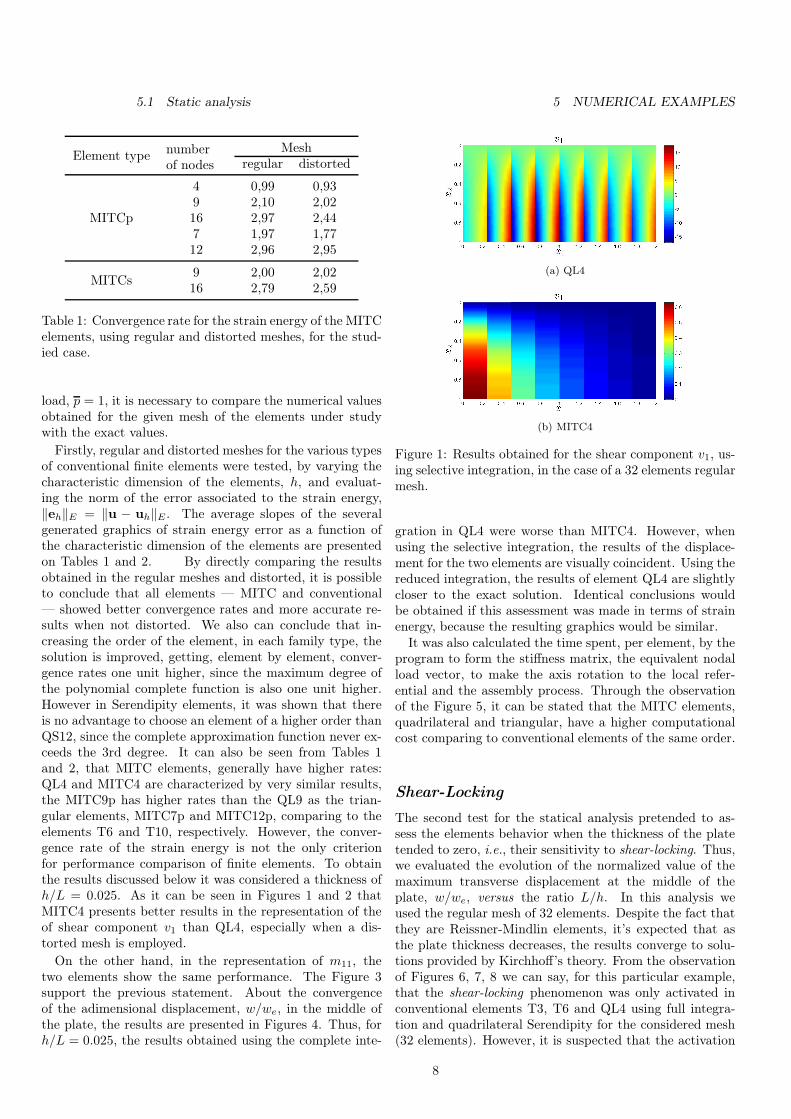
Table 1: Convergence rate for the strain energy of the MITCelements, using regular and distorted meshes, for the stud-ied case.

load, p = 1, it is necessary to compare the numerical valuesobtained for the given mesh of the elements under studywith the exact values.

Firstly, regular and distorted meshes for the various typesof conventional finite elements were tested, by varying thecharacteristic dimension of the elements, h, and evaluat-ing the norm of the error associated to the strain energy,‖eh‖E = ‖u − uh‖E . The average slopes of the severalgenerated graphics of strain energy error as a function ofthe characteristic dimension of the elements are presentedon Tables 1 and 2. By directly comparing the resultsobtained in the regular meshes and distorted, it is possibleto conclude that all elements — MITC and conventional— showed better convergence rates and more accurate re-sults when not distorted. We also can conclude that in-creasing the order of the element, in each family type, thesolution is improved, getting, element by element, conver-gence rates one unit higher, since the maximum degree ofthe polynomial complete function is also one unit higher.However in Serendipity elements, it was shown that thereis no advantage to choose an element of a higher order thanQS12, since the complete approximation function never ex-ceeds the 3rd degree. It can also be seen from Tables 1and 2, that MITC elements, generally have higher rates:QL4 and MITC4 are characterized by very similar results,the MITC9p has higher rates than the QL9 as the trian-gular elements, MITC7p and MITC12p, comparing to theelements T6 and T10, respectively. However, the conver-gence rate of the strain energy is not the only criterionfor performance comparison of finite elements. To obtainthe results discussed below it was considered a thickness ofh/L = 0.025. As it can be seen in Figures 1 and 2 thatMITC4 presents better results in the representation of theof shear component v1 than QL4, especially when a dis-torted mesh is employed.

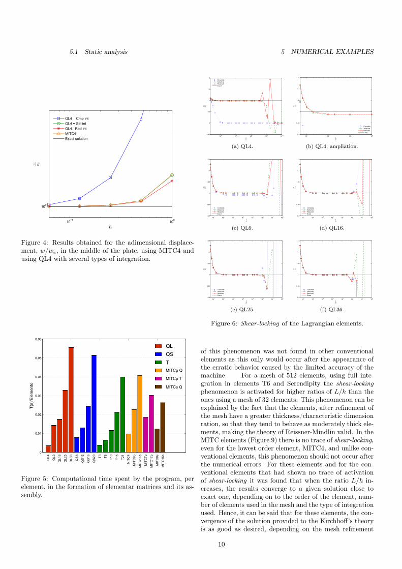
On the other hand, in the representation of m11, thetwo elements show the same performance. The Figure 3support the previous statement. About the convergenceof the adimensional displacement, w/we, in the middle ofthe plate, the results are presented in Figures 4. Thus, forh/L = 0.025, the results obtained using the complete inte-

(a) QL4

(b) MITC4

Figure 1: Results obtained for the shear component v1, us-ing selective integration, in the case of a 32 elements regularmesh.

gration in QL4 were worse than MITC4. However, whenusing the selective integration, the results of the displace-ment for the two elements are visually coincident. Using thereduced integration, the results of element QL4 are slightlycloser to the exact solution. Identical conclusions wouldbe obtained if this assessment was made in terms of strainenergy, because the resulting graphics would be similar.

It was also calculated the time spent, per element, by theprogram to form the stiffness matrix, the equivalent nodalload vector, to make the axis rotation to the local refer-ential and the assembly process. Through the observationof the Figure 5, it can be stated that the MITC elements,quadrilateral and triangular, have a higher computationalcost comparing to conventional elements of the same order.

Shear-Locking

The second test for the statical analysis pretended to as-sess the elements behavior when the thickness of the platetended to zero, i.e., their sensitivity to shear-locking. Thus,we evaluated the evolution of the normalized value of themaximum transverse displacement at the middle of theplate, w/we, versus the ratio L/h. In this analysis weused the regular mesh of 32 elements. Despite the fact thatthey are Reissner-Mindlin elements, it’s expected that asthe plate thickness decreases, the results converge to solu-tions provided by Kirchhoff’s theory. From the observationof Figures 6, 7, 8 we can say, for this particular example,that the shear-locking phenomenon was only activated inconventional elements T3, T6 and QL4 using full integra-tion and quadrilateral Serendipity for the considered mesh(32 elements). However, it is suspected that the activation

8

5 NUMERICAL EXAMPLES 5.1 Static analysis

Elementtype

numberof nodes

MeshRegular Distorted

Integration Integration

complete selective reduced complete selective reduced

QL

4 0,91 1,00 1,00 0,71 0,94 0,959 1,96 2,00 2,01 1,75 1,92 1,9416 2,94 2,91 3,09 2,58 2,71 2,6925 3,37 3,25 4,03 2,62 3,18 2,4036 3,13 2,84 3,45 1,83 1,92 1,81

QS

8 1,96 2,03 2,05 1,79 2,20 2,2512 2,89 2,91 2,92 2,68 2,73 2,7316 2,92 2,92 2,92 2,68 2,72 2,7220 2,92 2,92 2,92 2,68 2,72 2,72

T

3 0,90 — — 0,53 — —6 1,97 — — 1,71 — —10 2,87 — — 2,50 — —15 3,77 — — 2,65 — —21 2,97 — — 2,57 — —

Table 2: Convergence rate for the strain energy of the different conventional elements with different types of integrations,using regular and distorted meshes, to the studied case.

(a) QL4

(b) MITC4

Figure 2: Results obtained for the shear component v1, inthe case of a 32 elements distorted mesh.

(a) QL4

(b) MITC4

Figure 3: Results obtained for m11, using selective integra-tion, in the case of a 32 elements distorted mesh.

9

5.1 Static analysis 5 NUMERICAL EXAMPLES

101

100

100

h

w we

QL4 Cmp int

QL4 Sel int

QL4 Red int

MITC4

Exact solution

Figure 4: Results obtained for the adimensional displace-ment, w/we, in the middle of the plate, using MITC4 andusing QL4 with several types of integration.

0

0.01

0.02

0.03

0.04

0.05

0.06

QL4

QL9

QL16

QL25

QL36

QS

8

QS

12

QS

16

QS

20

T3

T6

T10

T15

T21

MIT

C4

MIT

C9p

MIT

C16p

MIT

C7p

MIT

C12p

MIT

C9s

MIT

C16s

T(s

)/E

lem

ento

QL

QS

T

MITCp Q

MITCp T

MITCs Q

Figure 5: Computational time spent by the program, perelement, in the formation of elementar matrices and its as-sembly.

102

104

106

108

1010

0.5

0

0.5

1

1.5

2

L

h

w we

Complete

Selective

Reduced

Exact

(a) QL4.

101

102

103

104

0.9

0.95

1

1.05

1.1

1.15

L

h

w we

Complete

Selective

Reduced

Exact

(b) QL4, ampliation.

101

102

103

104

105

106

107

108

0.9

0.95

1

1.05

1.1

1.15

L

h

w we

Complete

Selective

Reduced

Exact

(c) QL9.

101

102

103

104

105

106

107

108

0.9

0.95

1

1.05

1.1

1.15

L

h

w we

Complete

Selective

Reduced

Exact

(d) QL16.

101

102

103

104

105

106

107

108

0.9

0.95

1

1.05

1.1

1.15

L

h

w we

Complete

Selective

Reduced

Exact

(e) QL25.

101

102

103

104

105

106

107

108

0.9

0.95

1

1.05

1.1

1.15

L

h

w we

Complete

Selective

Reduced

Exact

(f) QL36.

Figure 6: Shear-locking of the Lagrangian elements.

of this phenomenon was not found in other conventionalelements as this only would occur after the appearance ofthe erratic behavior caused by the limited accuracy of themachine. For a mesh of 512 elements, using full inte-gration in elements T6 and Serendipity the shear-lockingphenomenon is activated for higher ratios of L/h than theones using a mesh of 32 elements. This phenomenon can beexplained by the fact that the elements, after refinement ofthe mesh have a greater thickness/characteristic dimensionration, so that they tend to behave as moderately thick ele-ments, making the theory of Reissner-Mindlin valid. In theMITC elements (Figure 9) there is no trace of shear-locking,even for the lowest order element, MITC4, and unlike con-ventional elements, this phenomenon should not occur afterthe numerical errors. For these elements and for the con-ventional elements that had shown no trace of activationof shear-locking it was found that when the ratio L/h in-creases, the results converge to a given solution close toexact one, depending on to the order of the element, num-ber of elements used in the mesh and the type of integrationused. Hence, it can be said that for these elements, the con-vergence of the solution provided to the Kirchhoff’s theoryis as good as desired, depending on the mesh refinement

10

5 NUMERICAL EXAMPLES 5.1 Static analysis

101

102

103

104

105

106

107

108

0

0.2

0.4

0.6

0.8

1

L

h

w we

Complete

Selective

Reduced

Exact

(a) QS8.

102

104

106

108

1010

0

0.2

0.4

0.6

0.8

1

L

h

w we

Complete

Selective

Reduced

Exact

(b) QS12.

102

104

106

108

1010

0

0.2

0.4

0.6

0.8

1

L

h

w we

Complete

Selective

Reduced

Exact

(c) QS16.

102

104

106

108

1010

0

0.2

0.4

0.6

0.8

1

L

h

w we

Complete

Selective

Reduced

Exact

(d) QS20.

Figure 7: Shear-locking of the Serendipity elements.

102

104

106

108

1010

0

0.2

0.4

0.6

0.8

1

L

h

w we

T3

T6

T10

T15

T21

Exact

(a) T.

101

102

103

104

105

106

107

0.9

0.95

1

1.05

1.1

1.15

L

h

w we

3

6

10

15

21

Exact

(b) T, ampliation.

Figure 8: Shear-locking of the triangular elements.

101

102

103

104

105

106

107

108

0.9

0.95

1

1.05

1.1

1.15

L

h

w we

MITC4p

MITC9p

MITC16p

MITC7p

MITC12p

E

(a) MITCp.

101

102

103

104

105

106

107

108

0.9

0.95

1

1.05

1.1

1.15

L

h

w we

MITC4s

MITC9s

MITC16s

E

(b) MITCs.

Figure 9: Shear-locking of MITC elements.

101

102

0.9

0.92

0.94

0.96

0.98

1

1.02

Laje R-M

Laje R-M with rot I

Laje K

Laje with rot I

Lh

ω

(a) Fundamental mode.

101

102

0.6

0.65

0.7

0.75

0.8

0.85

0.9

0.95

1

1.05

Laje R-M

Laje R-M with rot I

Laje K

Laje with rot I

Lh

ω

(b) Sixth mode.

Figure 10: Adimensional frequency vibrations. In the caseof the Reissner-Mindlin elements, a regular mesh with 128MITC16p elements was used.

used for each element type and each integration rule.

Free-vibration analysis

For the free vibration analysis, it was evaluated the con-vergence of the numerical values of the natural vibrationfrequency obtained from the study of the finite elementswith respect to the exact solution. The results obtainedusing the finite elements are presented on Tables 3 and 4.Selective integration was employed in the case of conven-tional elements.

For each mode, one may conclude that increasing theorder of the element, in each family type, the solution isimproved, getting, element by element, convergence ratesone unit higher, since the maximum degree of the polyno-mial complete function is also one unit higher. However,once again, it is shown that it isn’t worthwhile to use aSerendipity element higher than QS12. Furthermore, forthe higher modes, the convergence rates tends, in general,to slightly decrease, which can be explained by the greaterdifficulty of representing these modes. In contrast to whatis usual in the literature, in the present formulation, in ad-dition to the usual terms of the inertia associated to thetranslation, it was also considered the related terms associ-ated with the rotation. Thus, it was possible to carry out astudy to assess its importance in the behavior of the vibra-tion of the plate. For each of the plate theories (moderatelythick and thin) it was found that this influence is smaller, asthe plate becomes thinner. Besides, the frequency vibrationvalues obtained are smaller for the same ratio h/L, whenconsidering the terms in question, since in these situationsthe number of terms due to the mass is higher. This state-ments are supported by the results presented in Figure 10.

Linear stability analysis

The problem of linear stability analysis shows a similar for-mat to the problem of free vibration analysis: consists insolving a problem of eigenvalues and eigenvectors. How-ever the geometric matrix has a fundamental difference forthe mass matrix: in its definition appear first derivatives

11

5.1 Static analysis 5 NUMERICAL EXAMPLES

Element type numberof nodes

Modes1 2 3 4 5 6

QL

4 2,08 2,14 2,39 2,22 2,33 2,059 3,97 3,93 3,90 3,90 3,89 3,6716 5,95 5,94 5,84 5,78 5,78 5,7225 7,97 7,90 7,74 7,72 7,77 7,6636 6,39 9,86 9,63 9,63 9,69 9,53

QS

8 4,03 4,30 3,97 3,90 3,99 3,8912 6,94 6,29 6,12 5,79 6,02 5,7616 6,16 6,17 6,32 6,44 6,42 6,4320 6,84 6,31 6,25 6,04 6,00 6,23

T

3 1,77 1,75 2,10 2,08 1,94 1,916 3,80 3,78 3,62 3,71 3,59 3,6110 6,07 5,69 5,77 5,74 5,65 5,5715 7,97 7,87 7,41 7,46 7,41 7,3121 9,76 9,27 9,77 9,72 9,49 9,45

Table 3: Convergence rate for frequency vibration, using conventional elements, for the studied case.

Element typenumberof nodes

Modes1 2 3 4 5 6

MITCp

4 2,03 2,16 2,45 2,35 2,35 2,059 3,94 3,90 3,83 3,68 3,79 3,8116 6,17 5,99 5,49 5,69 5,69 5,427 3,94 3,87 3,59 3,68 3,74 3,6212 5,48 5,93 5,85 5,86 5,68 5,63

MITCs9 3,97 3,94 3,91 3,90 3,90 3,7316 5,20 5,94 5,84 5,78 5,78 5,72

Table 4: Convergence rate for frequency vibration, using MITC elements, for the studied case.

Element typenumberof nodes

Modes1 2 3 4 5 6

QL

4 2,01 2,02 2,07 2,10 2,03 2,059 3,99 3,99 3,96 3,95 3,95 3,9416 5,93 5,92 5,82 5,78 5,77 5,7125 7,90 7,89 7,69 7,96 7,78 7,7936 6,62 9,85 9,59 10,15 9,52 9,45

QS

8 3,99 4,03 4,00 3,93 4,03 3,9712 6,07 6,06 6,08 6,00 5,94 5,9516 5,91 6,07 6,13 5,58 5,19 5,1620 6,07 6,17 6,28 5,95 5,87 6,41

T

3 1,96 1,91 1,95 2,01 1,97 1,916 3,97 3,96 3,94 3,95 3,93 3,9210 5,96 5,97 5,96 5,97 5,96 5,9315 7,82 7,84 7,80 7,81 7,78 7,7921 8,96 9,78 9,66 10,05 9,61 9,50

Table 5: Convergence rates for instability loads, using conventional elements, for the studied case.

12

A MITC APPROXIMATION FUNCTIONS

of the approximation functions and not the approximationfunctions per se. Thus, generally, the results are similarand the elements tend to the same theoretical convergencerates, Tables 5 and 6. Selective integration was employedin the case of conventional elements.

The behavior of the elements in the various modes mayalso be extrapolated from the first mode of instability, de-spite the approximation quality begins to deteriorate forhigher modes. However, when using selective or reducedintegration in Lagrangian elements, in this analysis, it isnecessary to make a careful selection of the obtained modesfrom the program, since the selective integration of theseparticular elements is associated to an activation of spuri-ous modes. The frequencies associated to these modes aretotally erroneous. This behavior does not occur in Serendip-ity elements. When full integration is used, this problemceases to exist, but the accuracy of the results and con-vergence rates of approximation errors are lower than theones obtained with selective integration. The differencesbetween the results of the two types of integration will in-crease as the plate gets thinner. In the MITC elements wedon’t have this kind of problem.

6 Conclusions

The mixed finite element formulation can be understoodas an extension of the principle of stationarity of the to-tal potential energy, where we have as variables generalizedstreeses and deformations, besides the displacements. Inthis paper, we present a formulation based on mixed fieldsu, γ and λ

˜. This mixed formulation led to a general form

to evaluate the stiffness matrix Kss, valid for all three typesof MITC elements. Thus, it was concluded that using thetraditional formulation is very similar to use a mixed for-mulation where the distortion vector, γ, is directly approxi-mated. The only difference is that, instead of Kss, it’s usedKss.

The mixed formulation also explains the use of selectiveintegration in conventional quadrilateral elements. It canbe demonstrated for these elements that Kred

ss = Kss, whichmeans that the selective integration is not more than themixed formulation of these elements assuming certain ap-proximation functions for γ and λ. Although this result iswell known for other types of alternative formulations, thededuction presented here is original.

However, despite the selective integration of conventionalquadrilateral elements have the same variational bases thatthe MITC elements, their functions approximations to γ

and λ are different. It should be noted that sometimes,the first ones present spurious modes, while the secondsdon’t. Hence, it can be said that the mixed formulation isdependent on the choice of the approximation functions.

Summing up the numerical results, it can be stated thatthe MITC elements, despite the higher computational cost,have several advantages over conventional elements:

(i) they don’t suffer from shear-locking;

(ii) they don’t display spurious modes;

(iii) all elements, except element MITC9p, pass the bend-ing, shear and twisting patch tests. In the case theMITC9p, the test is almost passed;

(iv) the representation of the shear components on staticanalysis converges quickly to the exact solution;

(v) show a slightly higher rate of convergence in terms ofthe norm of the strain energy error.

These conclusions remain valid regardless of the degree ofdistortion of the mesh considered.

A MITC approximation functions

Approximation functions for MITC9p:

Ψu =

ΨQS8 O O

O ΨQL9 O

O O ΨQL9

(85a)

Φγ1 =[1 ξ1 ξ2 ξ1ξ2 ξ22

](85b)

Φλ

˜1 =[δ (ξ − ξ1) δ (ξ − ξ2) δ (ξ − ξ3) δ (ξ − ξ4) 1

].

(85c)

Approximation functions for MITC16p:

Ψu =

Ψw,M16p O O

O ΨQL16 O

O O ΨQL16

(86a)

Φγ1 =[1 ξ1 ξ2 ξ21 ξ1ξ2 ξ22 ξ21ξ2 ξ1ξ

22 ξ32

]

(86b)

Φλ

˜1 =[δ (ξ − ξ1) δ (ξ − ξ2) δ (ξ − ξ3) δ (ξ − ξ4)

δ (ξ − ξ5) δ (ξ − ξ6) 1 ξ1 ξ2].

(86c)

Approximation functions for MITC7p:

Ψu =

ΨT6 O O

O Ψθ,M7p O

O O Ψθ,M7p

(87a)

Ψγ =

[1 ξ1 ξ2 0 0 0 ξ1ξ2 ξ220 0 0 1 ξ1 ξ2 −ξ21 −ξ1ξ2

](87b)

Ψλ

˜ =

[δ (ξ − ξ1) δ (ξ − ξ2) −

√22 δ (ξ − ξ3)

0 0√22 δ (ξ − ξ3)

. . .

. . .−

√22 δ (ξ − ξ4) 0 0 1 0

√22 δ (ξ − ξ4) −δ (ξ − ξ5) δ (ξ − ξ6) 0 1

].

(87c)

13

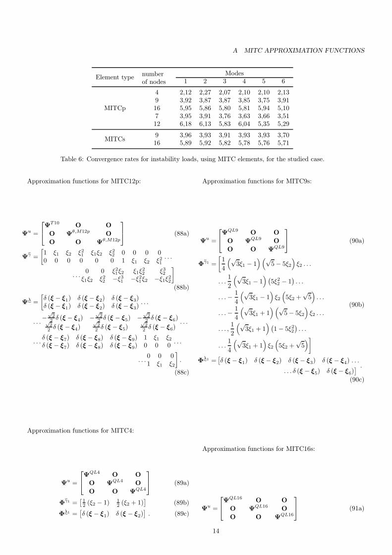
A MITC APPROXIMATION FUNCTIONS

Element type numberof nodes

Modes1 2 3 4 5 6

MITCp

4 2,12 2,27 2,07 2,10 2,10 2,139 3,92 3,87 3,87 3,85 3,75 3,9116 5,95 5,86 5,80 5,81 5,94 5,107 3,95 3,91 3,76 3,63 3,66 3,5112 6,18 6,13 5,83 6,04 5,35 5,29

MITCs9 3,96 3,93 3,91 3,93 3,93 3,7016 5,89 5,92 5,82 5,78 5,76 5,71

Table 6: Convergence rates for instability loads, using MITC elements, for the studied case.

Approximation functions for MITC12p:

Ψu =

ΨT10 O O

O Ψθ,M12p O

O O Ψθ,M12p

(88a)

Ψγ =

[1 ξ1 ξ2 ξ21 ξ1ξ2 ξ22 0 0 0 00 0 0 0 0 0 1 ξ1 ξ2 ξ21

. . .

. . .0 0 ξ21ξ2 ξ1ξ

22 ξ32

ξ1ξ2 ξ22 −ξ31 −ξ21ξ2 −ξ1ξ22

]

(88b)

Ψλ

˜ =

[δ (ξ − ξ1) δ (ξ − ξ2) δ (ξ − ξ3)δ (ξ − ξ1) δ (ξ − ξ2) δ (ξ − ξ3)

. . .

. . .−

√22 δ (ξ − ξ4) −

√22 δ (ξ − ξ5) −

√22 δ (ξ − ξ6)√

22 δ (ξ − ξ4)

√22 δ (ξ − ξ5)

√22 δ (ξ − ξ6)

. . .

. . .δ (ξ − ξ7) δ (ξ − ξ8) δ (ξ − ξ9) 1 ξ1 ξ2δ (ξ − ξ7) δ (ξ − ξ8) δ (ξ − ξ9) 0 0 0

. . .

. . .0 0 01 ξ1 ξ2

].

(88c)

Approximation functions for MITC4:

Ψu =

ΨQL4 O O

O ΨQL4 O

O O ΨQL4

(89a)

Φγ1 =[12 (ξ2 − 1) 1

2 (ξ2 + 1)]

(89b)

Φλ

˜1 =[δ (ξ − ξ1) δ (ξ − ξ2)

]. (89c)

Approximation functions for MITC9s:

Ψu =

ΨQL9 O O

O ΨQL9 O

O O ΨQL9

(90a)

Φγ1 =

[1

4

(√3ξ1 − 1

)(√5− 5ξ2

)ξ2 . . .

. . .1

2

(√3ξ1 − 1

) (5ξ22 − 1

). . .

. . .− 1

4

(√3ξ1 − 1

)ξ2

(5ξ2 +

√5). . .

. . .− 1

4

(√3ξ1 + 1

)(√5− 5ξ2

)ξ2 . . .

. . . ,1

2

(√3ξ1 + 1

) (1− 5ξ22

). . .

. . .1

4

(√3ξ1 + 1

)ξ2

(5ξ2 +

√5)]

(90b)

Φλ

˜1 =[δ (ξ − ξ1) δ (ξ − ξ2) δ (ξ − ξ3) δ (ξ − ξ4) . . .

. . . δ (ξ − ξ5) δ (ξ − ξ6)] .

(90c)

Approximation functions for MITC16s:

Ψu =

ΨQL16 O O

O ΨQL16 O

O O ΨQL16

(91a)

14

A MITC APPROXIMATION FUNCTIONS

Φγ1 =

[(√5− 5ξ1

)ξ1(c− ξ2)(c+ ξ2)(d− ξ2)

4 (d3 − c2d). . .

. . .

(√5− 5ξ1

)ξ1(c− ξ2)(d − ξ2)(d+ ξ2)

4c(c− d)(c + d). . .

. . .

(√5− 5ξ1

)ξ1(c+ ξ2)(d − ξ2)(d+ ξ2)

4c(c− d)(c + d). . .

. . .

(√5− 5ξ1

)ξ1(c− ξ2)(c+ ξ2)(d+ ξ2)

4 (d3 − c2d). . .

. . .

(1− 5ξ21

) (ξ22 − c2

)(d− ξ2)

2 (d3 − c2d). . .

. . .

(1− 5ξ21

)(c− ξ2)

(ξ22 − d2

)

2 (c3 − cd2). . .

. . .

(1− 5ξ21

)(c+ ξ2)

(ξ22 − d2

)

2 (c3 − cd2). . .

. . .

(1− 5ξ21

) (ξ22 − c2

)(d+ ξ2)

2 (d3 − c2d). . .

. . .ξ1

(5ξ1 +

√5)(c− ξ2)(c+ ξ2)(d− ξ2)

4d(c− d)(c + d). . .

. . .ξ1

(5ξ1 +

√5)(c− ξ2)

(ξ22 − d2

)

4 (c3 − cd2). . .

. . .ξ1

(5ξ1 +

√5)(c+ ξ2)

(ξ22 − d2

)

4 (c3 − cd2). . .

. . .ξ1

(5ξ1 +

√5)(c− ξ2)(c+ ξ2)(d+ ξ2)

4d(c− d)(c + d)

]

(91b)

Φλ

˜1 = [δ (ξ − ξ1) δ (ξ − ξ2) δ (ξ − ξ3) δ (ξ − ξ4) . . .

. . . δ (ξ − ξ5) δ (ξ − ξ6) δ (ξ − ξ7) . . .

. . . δ (ξ − ξ8) δ (ξ − ξ9) δ (ξ − ξ10) . . .

. . . δ (ξ − ξ11) δ (ξ − ξ12)] .

(91c)

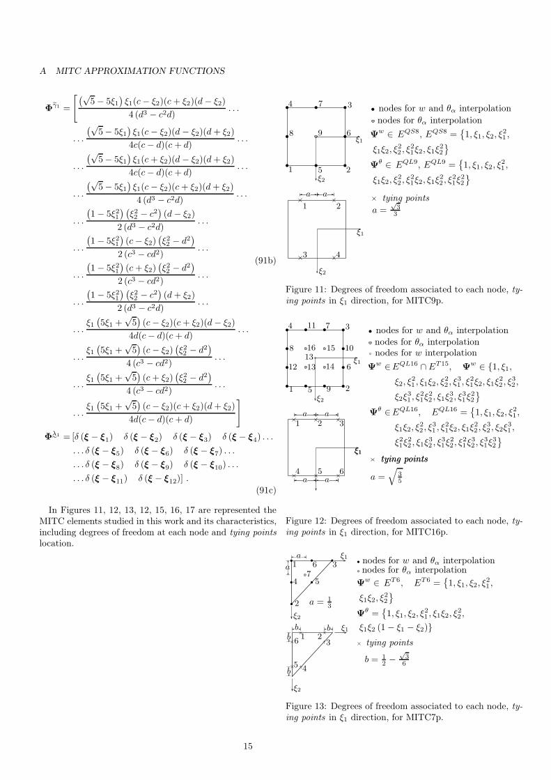
In Figures 11, 12, 13, 12, 15, 16, 17 are represented theMITC elements studied in this work and its characteristics,including degrees of freedom at each node and tying pointslocation.

ξ1

ξ1

ξ2

ξ2

nodes for w and θα interpolation

nodes for θα interpolation

aa

a =√33

Ψw ∈ EQS8, EQS8 =1, ξ1, ξ2, ξ

21 ,

ξ1ξ2, ξ22 , ξ

21ξ2, ξ1ξ

22

Ψθ ∈ EQL9, EQL9 =1, ξ1, ξ2, ξ

21 ,

ξ1ξ2, ξ22 , ξ

21ξ2, ξ1ξ

22 , ξ

21ξ

22

1

1

2

2

3

3

4

4

5

6

7

8 9

tying points

Figure 11: Degrees of freedom associated to each node, ty-ing points in ξ1 direction, for MITC9p.

ξ1

ξ1

ξ1

ξ2

nodes for w and θα interpolation

nodes for θα interpolationnodes for w interpolation

aa

aa

a =√

35

Ψw ∈EQL16 ∩ ET15, Ψw ∈ 1, ξ1,ξ2, ξ

21 , ξ1ξ2, ξ

22 , ξ

31 , ξ

21ξ2, ξ1ξ

22 , ξ

32 ,

ξ2ξ31 , ξ

21ξ

22 , ξ1ξ

32 , ξ

31ξ

22

Ψθ ∈EQL16, EQL16 =1, ξ1, ξ2, ξ

21 ,

ξ1ξ2, ξ22 , ξ

31 , ξ

21ξ2, ξ1ξ

22 , ξ

32 , ξ2ξ

31 ,

ξ21ξ22 , ξ1ξ

32 , ξ

31ξ

22 , ξ

21ξ

32 , ξ

31ξ

32

1

1

2

2

3

3

4

4

5

5

6

6

7

8

9

10

11

12

13

13 14

1516

tying pointstying points

Figure 12: Degrees of freedom associated to each node, ty-ing points in ξ1 direction, for MITC16p.

ξ1

ξ1

ξ2

ξ2

nodes for w and θα interpolationnodes for θα interpolationa

a

a = 13

b

bb

b

b = 12 −

√36

Ψw ∈ ET6, ET6 =1, ξ1, ξ2, ξ

21 ,

ξ1ξ2, ξ22

Ψθ =1, ξ1, ξ2, ξ

21 , ξ1ξ2, ξ

22 ,

ξ1ξ2 (1− ξ1 − ξ2)

1

1

2

2

3

3

4

4

5

5

6

6

7

tying points

Figure 13: Degrees of freedom associated to each node, ty-ing points in ξ1 direction, for MITC7p.

15

A MITC APPROXIMATION FUNCTIONS

ξ1

ξ1

ξ2

ξ2

nodes for w and θα interpolationnodes for θα interpolationnodes for w interpolation

a

a

a = 13

b

b

c

c

cc

c =√

320

b = 14

Ψw ∈ ET10, ET10 =1, ξ1, ξ2, ξ

21 ,

ξ1ξ2, ξ22 , ξ

31 , ξ

21ξ2, ξ1ξ

22 , ξ

32

Ψθ =1, ξ1, ξ2, ξ

21 , ξ2ξ1, ξ

22 , ξ

31 , ξ2ξ

21 ,

ξ22ξ1, ξ32 , ξ2ξ

21(ξ2 + ξ1), ξ

22ξ1(ξ2 + ξ1)

1

1

2

2

3

3

4

4

5

5

6

6

7

7

8

8

9

9

10

10

11

12

tying points

Figure 14: Degrees of freedom associated to each node, ty-ing points in ξ1 direction, for MITC12p.

ξ1

ξ1

ξ2

ξ21

1

2

2

34

tying points

nodes for w and θα interpolation

Ψw,Ψθ ∈ EQL4,

EQL4 = 1, ξ1, ξ2, ξ1ξ2

Figure 15: Degrees of freedom associated to each node, ty-ing points in ξ1 direction, for MITC4.

ξ1

ξ1

ξ2

ξ2

nodes for w and θα interpolation

aa

b

b a =√33

b =√

35

Ψw,Ψθ ∈ EQL9, EQL9 = 1, ξ1, ξ2,ξ21 , ξ1ξ2, ξ

22 , ξ

21ξ2, ξ1ξ

22 , ξ

21ξ

22

1

1

2

2

3

3

4

4

5

5

6

6

7

8 9

tying points

Figure 16: Degrees of freedom associated to each node, ty-ing points in ξ1 direction, for MITC9s.

ξ1

ξ1

ξ2

ξ2

nodes for w and θα interpolation

aa

b

b

c

c

a =√

35

b =

√30−

√480

70

c =

√30+

√480

70

Ψw,Ψθ ∈ EQL16, EQL16 = 1, ξ1, ξ2,ξ21 , ξ1ξ2, ξ

22 , ξ

31 , ξ

21ξ2, ξ1ξ

22 , ξ

32 , ξ

31ξ2,

ξ21ξ22 , ξ1ξ

32 , ξ

31ξ

32

1

1

2

2

3

3

4

4

5

5

6

6

7

7

8

8

9

9

10

10

11

11

12

12

13 14

1516

tying points

Figure 17: Degrees of freedom associated to each node, ty-ing points in ξ1 direction, for MITC16s.

16

REFERENCES REFERENCES

References

Bathe, K.-J. (1996). Finite Element Procedures. PrenticeHall.

Dvorkin, E. N. and K.-J. Bathe (1984). A continuum me-chanics based four-node shell element for general non-linear analysis. Engineering Computations, 1 (1), 77–88.

Hinton, E. and H. C. Huang (1986). A family of quadrilat-eral Mindlin plate elements with substitute shear strainfields. Computers & Structures, 23 (3), 409–431.

17